This article was downloaded by:[INFLIBNET, India order 2005]On: 16 February 2008Access Details: [subscription number 772813341]Publisher: Taylor & FrancisInforma Ltd Registered in England and Wales Registered Number: 1072954Registered office: Mortimer House, 37-41 Mortimer Street, London W1T 3JH, UK

International Journal of ComputerMathematicsPublication details, including instructions for authors and subscription information:http://www.informaworld.com/smpp/title~content=t713455451

An application of real-coded genetic algorithm (formixed integer non-linear programming in an optimaltwo-warehouse inventory policy for deteriorating itemswith a linear trend in demand and a fixed planninghorizon)P. Pal a; C. B. Das b; A. Panda a; A. K. Bhunia aa Department of Computer Science, Midnapore College, W.B, Indiab Department of Mathematics, University of Burdwan, Burdwan, W.B, India

Online Publication Date: 01 February 2005To cite this Article: Pal, P., Das, C. B., Panda, A. and Bhunia, A. K. (2005) 'An application of real-coded genetic algorithm(for mixed integer non-linear programming in an optimal two-warehouse inventory policy for deteriorating items with alinear trend in demand and a fixed planning horizon)', International Journal of Computer Mathematics, 82:2, 163 - 175To link to this article: DOI: 10.1080/00207160412331296733URL: http://dx.doi.org/10.1080/00207160412331296733

PLEASE SCROLL DOWN FOR ARTICLE

Full terms and conditions of use: http://www.informaworld.com/terms-and-conditions-of-access.pdf

This article maybe used for research, teaching and private study purposes. Any substantial or systematic reproduction,re-distribution, re-selling, loan or sub-licensing, systematic supply or distribution in any form to anyone is expresslyforbidden.

The publisher does not give any warranty express or implied or make any representation that the contents will becomplete or accurate or up to date. The accuracy of any instructions, formulae and drug doses should beindependently verified with primary sources. The publisher shall not be liable for any loss, actions, claims, proceedings,demand or costs or damages whatsoever or howsoever caused arising directly or indirectly in connection with orarising out of the use of this material.

Dow

nloa

ded

By:

[IN

FLIB

NE

T, In

dia

orde

r 200

5] A

t: 07

:24

16 F

ebru

ary

2008

International Journal of Computer MathematicsVol. 82, No. 2, February 2005, 163–175

An application of real-coded genetic algorithm (for mixedinteger non-linear programming in an optimal two-warehouseinventory policy for deteriorating items with a linear trend in

demand and a fixed planning horizon)

P. PAL†, C. B. DAS‡, A. PANDA† and A. K. BHUNIA†*

†Department of Computer Science, Midnapore College, W.B., India‡Department of Mathematics, University of Burdwan, Burdwan 713104, W.B., India

(Revised 24 September 2003; in final form 11 July 2004)

The purpose of this research is to discuss an application of real-coded Genetic Algorithm (RCGA) formixed integer non-linear programming in a two-warehouses inventory control problem. Our objectiveis to determine an optimal replenishment number, lot-size of a two-warehouse (owned and rented ware-house (RW)) inventory system for deteriorating items removing the impractical assumption regardingthe storage capacity of RW. The model is formulated with infinite replenishment, finite planninghorizon, linearly time dependent demand (increasing) and partially backlogged shortages. The mathe-matical formulation of the problem indicates that the model is a constrained non-linear mixed integerproblem with one integer and one non-integer variables. To solve this problem, we develop a RCGAwith ranking selection, whole arithmetic crossover and mutation (uniform mutation for integer variableand non-uniform for non-integer variable). The proposed model has been solved using this RCGA andillustrated with four numerical examples.

Keywords: Genetic algorithm; Two-warehouses inventory; Deterioration; Partial backlogging; Finiteplanning horizon

C.R. Categories: F.2.2; I.1.2; I.2.8

1. Introduction

Normally, the decision-making problems are formulated as constrained/unconstrained non-linear optimization problem which are solved by traditional direct and gradient basedoptimization method. These methods have some limitations. Among these limitations, oneis that the traditional non-linear optimization methods very often stuck to the local optimum.To overcome some of these limitations, during last 40 years, attempt has been made to solvethe problem on the basis of the principle of evaluation and hereditary. Such system has someselection process based on the fitness of individuals and some genetic operations. Recently,these types of methods such as Genetic Algorithm (GA), Simulated Annealing and Tabu

*Corresponding author. Email: bhuniaak@rediffmail.com

International Journal of Computer MathematicsISSN 0020-7160 print/ISSN 1029-0265 online © 2005 Taylor & Francis Ltd

http://www.tandf.co.uk/journalsDOI: 10.1080/00207160412331296733

Dow

nloa

ded

By:

[IN

FLIB

NE

T, In

dia

orde

r 200

5] A

t: 07

:24

16 F

ebru

ary

2008

164 P. Pal et al.

search, which are known as soft computing method, are used for solving decision-makingproblems. Among these methods, GA is very popular. It is a stochastic search method foroptimization problems on the basis of the mechanics of natural selection and natural genetics,i.e., the principle of evolution ‘Survival of the fittest’. It is executed iteratively on the set ofreal/binary-coded solution called population. In each iteration, three basic genetic operations,i.e., selection/reproduction, crossover and mutation are performed.

This algorithm was developed by Holland in the year 1975. There is an inherent parallelism,because GA searches from a set of solutions and not from a single one. It has demonstrated con-siderable success in providing good solutions to many complex optimization problems. Whenthe objective functions are multi-modal or the search space is partially irregular, algorithmsare to be highly robust so as to avoid getting struck to the optimal solution. The advantageof GA is to obtain the global solution fairly. GA has been well discussed and summarizedby several authors, i.e., Goldberg [1], Michalewicz [2] and Sakawa [3]. Recently, GA hasbeen successfully applied to a wide variety of problems such as Traveling Salesman prob-lems [4], Scheduling problems [5] and Numerical optimization [6, 7]. Till date, only a veryfew researchers have applied it to solve the problem in the field of inventory control system.Among them, one may refer to the work of Khouja et al. [8], Sarkar and Charles [9], Mandaland Maiti [10], and Yokoyama and Lewis [11] among others.

In the existing literature of inventory control, it is observed that the traditional inventorymodels have been developed mainly for single warehouse under the basic assumption: theavailable warehouse of management has unlimited storage space. In practice, this assumptionis not viable, because any warehouse has finite storage space. However, for economical benefit,the inventory management are interested to maintain a rented warehouse (RW) in addition tothe owned one with limited storage space; particularly, when the inventory related cost forprocurement (i.e., ordering cost, transportation cost for replenishment, administrative cost,etc.) is relatively expensive than using RW, discount for bulk purchase is very much attractive,or demands are very high.

In the recent years, the two-warehouse inventory problems have received considerableattention from several researchers. They have developed different types of two-warehousesinventory model for deteriorating and non-deteriorating items. To get an idea of the trend ofrecent research, one may refer to the works of Goswami and Chaudhuri [12], Bhunia andMaiti [13, 14], Pakkala and Achary [15], Benkherouf [16], Lee and Ma [17], Kar et al. [18]and others. All these models except those of Lee and Ma [17] and Kar et al. [18] have beendeveloped for single replenishment cycle considering the cycle length as prescribed or fordecision variable. Another assumption is that the cycle will be repeated infinitely. However,this is not always true. It is worth mentioning that the production of food grains such as paddy,rice and wheat is periodical through out the world. Normally, in those countries where thestate control is less, the demand of essential food grains is lower at the time of harvest andrises to the highest level just before the next harvest. This phenomenon is very common indeveloping third world countries where most of the people are landless (small farmers andland laborers) or marginal farmers. They produced food grains by cultivating either their ownland and/or the land of a landlord by sharing at a certain ratio. For various reasons, some ofthem are forced to sell a part of their product and buy grains from the open market after theconsumption of their own grains. As a result, the demand rate of food grains remains partlyconstant and increases partly with time for a fixed planning horizon (i.e., for a calendar year).

In the last few years, many researchers have paid considerable attention on inventory prob-lems with fixed planning horizon and deterministic time varying demand pattern. In thisconnection, the recent works of Goyal et al. [19], Chakrabarti and Chaudhuri [20] and Bhuniaand Maiti [21] among others are worth mentioning. All these models deal with the case ofsingle warehouse under unrealistic assumption regarding the storage space of the available

Dow

nloa

ded

By:

[IN

FLIB

NE

T, In

dia

orde

r 200

5] A

t: 07

:24

16 F

ebru

ary

2008

GA mixed integer non-linear programming 165

warehouse. Recently, very few researchers developed this type of problems considering twostorage facilities. Lee and Ma [17] developed a no-shortage inventory model for perishableitems with free form time dependent demand and fixed planning horizon. In their model,some cycles are of single warehouse system and the remaining is of two-warehouse system.Kar et al. [18] discussed two storage inventory problem for non-perishable items with lineartrend in demand over a fixed planning horizon considering lot-size dependent replenishment(ordering cost). In their models, all cycles are of two-warehouse system. However, both thesetwo-warehouse models were based on an impractical assumption that the RW has unlimitedcapacity.

In this article, we develop a finite planning horizon deterministic inventory model for dete-riorating items with two-warehouses (OW and RW) by removing the impractical assumptionregarding the storage capacity of RW. Owing to different preserving facilities and storageenvironment, inventory holding cost and deterioration rates are considered to be different indifferent warehouses. In addition, the replenishment cycle lengths are equal, the demand rateis a continuous linearly increasing function of time and the partially backlogged shortages areallowed in all cycles. Like Kar et al. [20], in each cycle, the replenishment cost is assumedto be dependent linearly on lot-size, and the stocks of RW are also transported to OW incontinuous release pattern. The model is formulated as a constrained non-linear mixed integerproblem with one integer and one non-integer variable. Considering the complexity of solvingsuch a model, we develop a real-coded GA (RCGA) for mixed variables (integer and non-integer) with ranking selection, whole arithmetic crossover and mutation. In whole arithmeticcrossover, convex combinations of genes corresponding to non-integer variable, and interme-diate value of genes corresponding to variable of two randomly selected chromosomes aretaken for crossover. To introduce the diversity in the genetics, uniform and non-uniform muta-tions are used for genes corresponding to the integer and non-integer variables, respectively.Finally, four numerical examples are presented to illustrate the results for different scenarios.

2. Assumptions and notations

The notations used in developing this model are as follows:

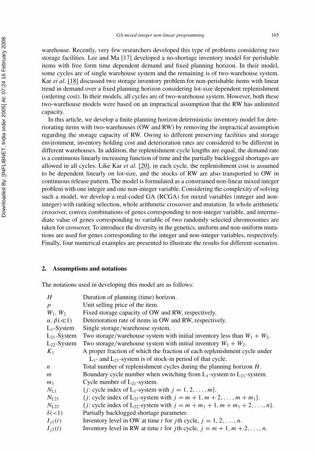
H Duration of planning (time) horizon.p Unit selling price of the item.W1, W2 Fixed storage capacity of OW and RW, respectively.α, β(�1) Deterioration rate of items in OW and RW, respectively.L1-System Single storage/warehouse system.L21-System Two storage/warehouse system with initial inventory less than W1 + W2.L22-System Two storage/warehouse system with initial inventory W1 + W2.K1 A proper fraction of which the fraction of each replenishment cycle under

L1- and L21-system is of stock-in period of that cycle.n Total number of replenishment cycles during the planning horizon H .m Boundary cycle number when switching from L1-system to L21-system.m1 Cycle number of L21-system.NL1 {j : cycle index of L1-system with j = 1, 2, . . . , m}.NL21 {j : cycle index of L21-system with j = m + 1, m + 2, . . . , m + m1}.NL22 {j : cycle index of L22-system with j = m + m1 + 1, m + m1 + 2, . . . , n}.δ(<1) Partially backlogged shortage parameter.Ij1(t) Inventory level in OW at time t for j th cycle, j = 1, 2, . . . , n.Ij2(t) Inventory level in RW at time t for j th cycle, j = m + 1, m + 2, . . . , n.

Dow

nloa

ded

By:

[IN

FLIB

NE

T, In

dia

orde

r 200

5] A

t: 07

:24

16 F

ebru

ary

2008

166 P. Pal et al.

QL1,j Initial inventory units for j th cycle, j = 1, 2, . . . , m.QL2,j Initial inventory units for j th cycle, j = m + 1, m + 2, . . . , n.BL,j Back-ordering units for j th cycle, j = 1, 2, . . . , n.SQL,j Shortage units held during the j th cycle, j = 1, 2, . . . , n.Iow,j Inventory units held in OW during the j th cycle, j = 1, 2, . . . , n.Irw,j Inventory units held in RW during the j th cycle, j = m + 1, m + 2, . . . , n.Dow,j Inventory units deteriorated in OW during the j th cycle, j = 1, 2, . . . , n.Drw,j Inventory units deteriorated in RW during the j th cycle, j = m + 1,

m + 2, . . . , n.Ct Transportation cost per unit for transferring the items from RW to OW.Cs Shortage cost per unit per unit time.Cp, Cd Lost sale and purchase cost per unit, respectively.Cow, Crw Inventory carrying cost in OW and in RW per unit per unit time, respectively.Qow, Qrw Total replenished quantity in OW and in RW for the entire planning horizon,

respectively.Qshort Total backlogged quantity for the entire planning horizon.

The proposed inventory model is developed under the following assumptions:

1. Replenishment rate is infinite and lead-time is constant.2. The inventory system operates for a prescribed planning horizon.3. All replenishment cycles are assumed to be of equal length. The period for which there is

no shortage in each interval of L1- and L21-system is a K1 fraction of the scheduling periodH/n, and is equal to K1H/n (0 < K1 ≤ 1).

4. Deterioration is considered only after the inventory is stored in the warehouse. There isneither repair nor replacement of the deteriorated units during the planning horizon.

5. Shortages, if any, are allowed and partially backlogged and cleared as soon as fresh stocksarrive.

6. Time lag between selling from OW and filling up the space by new units from RW isnegligible.

7. The units will be sold from OW and shifting the same amount from RW to OW will betransported immediately to fill up that space by new units in OW.

8. The demand rate f (t) at any instant t is a linear function of time, i.e., f (t) = a + bt, a, b ≥0.

9. The replenishment cost (ordering cost) FL,i for the ith cycle is linearly dependent on lot-sizeon that cycle and is in the following form.

FL,i = C1 + Cr1(QL1,j + BL,i), i ∈ NL1

= C1 + Cr1(W1 + BL,i) + Cr2(QL2,j − W1), i ∈ NL21

= C1 + Cr1(W1 + BL,i) + Cr2W2, i ∈ NL22,

where C1 is the fixed replenishment cost in each cycle and Cr1, Cr2(Cr1 < Cr2) theadditional replenishment cost per unit for replenishing the items in OW and RW,respectively.

3. Mathematical model

According to Assumption 3, the planning horizon has been divided into n equal parts of lengthH/n. Therefore, the reorder times over the planning horizon H will be tj,0 = (j − 1)H/n

Dow

nloa

ded

By:

[IN

FLIB

NE

T, In

dia

orde

r 200

5] A

t: 07

:24

16 F

ebru

ary

2008

GA mixed integer non-linear programming 167

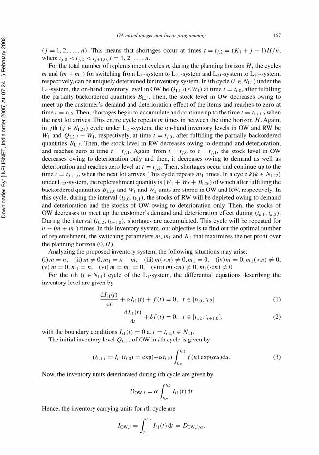
(j = 1, 2, . . . , n). This means that shortages occur at times t = tj,2 = (K1 + j − 1)H/n,where tj,0 < tj,2 < tj+1,0,j = 1, 2, . . . , n.

For the total number of replenishment cycles n, during the planning horizon H , the cyclesm and (m + m1) for switching from L1-system to L21-system and L21-system to L22-system,respectively, can be uniquely determined for inventory system. In ith cycle (i ∈ NL1) under theL1-system, the on-hand inventory level in OW be QL1,i (≤W1) at time t = ti,0, after fulfillingthe partially backordered quantities BL,i . Then, the stock level in OW decreases owing tomeet up the customer’s demand and deterioration effect of the items and reaches to zero attime t = ti,2. Then, shortages begin to accumulate and continue up to the time t = ti+1,0 whenthe next lot arrives. This entire cycle repeats m times in between the time horizon H . Again,in j th (j ∈ NL21) cycle under L21-system, the on-hand inventory levels in OW and RW beW1 and QL2,j − W1, respectively, at time t = tj,0, after fulfilling the partially backorderedquantities BL,j . Then, the stock level in RW decreases owing to demand and deterioration,and reaches zero at time t = tj,1. Again, from t = tj,0 to t = tj,1, the stock level in OWdecreases owing to deterioration only and then, it decreases owing to demand as well asdeterioration and reaches zero level at t = tj,2. Then, shortages occur and continue up to thetime t = tj+1,0 when the next lot arrives. This cycle repeats m1 times. In a cycle k(k ∈ NL22)

under L22-system, the replenishment quantity is (W1 + W2 + BL2k) of which after fulfilling thebackordered quantities BL2,k and W1 and W2 units are stored in OW and RW, respectively. Inthis cycle, during the interval (tk,0, tk,1), the stocks of RW will be depleted owing to demandand deterioration and the stocks of OW owing to deterioration only. Then, the stocks ofOW decreases to meet up the customer’s demand and deterioration effect during (tk,1, tk,2).During the interval (tk,2, tk+1,0), shortages are accumulated. This cycle will be repeated forn − (m + m1) times. In this inventory system, our objective is to find out the optimal numberof replenishment, the switching parameters m, m1 and K1 that maximizes the net profit overthe planning horizon (0,H).

Analyzing the proposed inventory system, the following situations may arise:(i) m = n, (ii) m �= 0, m1 = n − m, (iii) m(<n) �= 0, m1 = 0, (iv) m = 0, m1(<n) �= 0,(v) m = 0, m1 = n, (vi) m = m1 = 0, (viii) m(<n) �= 0, m1(<n) �= 0

For the ith (i ∈ NL1) cycle of the L1-system, the differential equations describing theinventory level are given by

dIi1(t)

dt+ αIi1(t) + f (t) = 0, t ∈ [ti,0, ti,2] (1)

dIi1(t)

dt+ δf (t) = 0, t ∈ [ti,2, ti+1,0], (2)

with the boundary conditions Ii1(t) = 0 at t = ti,2,i ∈ NL1.The initial inventory level QL1,i of OW in ith cycle is given by

QL1,i = Ii1(ti,0) = exp(−αti,0)

∫ ti,2

ti,0

f (u) exp(αu)du. (3)

Now, the inventory units deteriorated during ith cycle are given by

DOW,i = α

∫ ti,2

ti,0

Ii1(t) dt

Hence, the inventory carrying units for ith cycle are

IOW,i =∫ ti,2

ti,0

Ii1(t) dt = DOW,i/α.

Dow

nloa

ded

By:

[IN

FLIB

NE

T, In

dia

orde

r 200

5] A

t: 07

:24

16 F

ebru

ary

2008

168 P. Pal et al.

Again, the difference between the initial inventory and total selling during the interval [ti,0, ti,2]will be deteriorated units during ith cycle, i.e.,

DOW,i = QL1,i −∫ ti,2

ti,0

f (t) dt (4)

The total time units of backlogged quantities and the maximum level of shortages for ith cycleare given by

SQL,i = −∫ ti+1,0

ti,2

Ii1(t) dt (5)

and

BL,i = −Ii1(ti+1,0) = δ

∫ ti+1,0

ti,2

f (t) dt (6)

Again, for the j th (j ∈ NL21) cycle of L21-system, the differential equations governing theinventory system are given by

dIj2(t)

dt+ βIj2(t) + f (t) = 0, t ∈ [tj,0, tj,1] (7)

dIj1(t)

dt+ αIj1(t) = 0, t ∈ [tj,0, tj,1] (8)

dIj1(t)

dt+ αIj1(t) + f (t) = 0, t ∈ [tj,1, tj,2] (9)

dIj1(t)

dt+ δf (t) = 0, t ∈ [tj,2, tj+1,0] (10)

with the boundary conditions

Ij2(tj,1) = 0, Ij1(tj,0) = 0, Ij1(tj,2) = W1 (11)

In addition, Ij1(t) is continuous at t = tj1.Now, the initial total inventory level QL2,j of OW and RW in j th cycle is given by

QL2,j = W1 + Ij2(tj,0)

= W1 +∫ tj,1

tj,0

exp{β(u − tj,0)}f (u) du. (12)

The inventory deteriorated units and carrying units during j th cycle in RW and OW can becalculated similarly as in L1-system.

In addition, the expressions for SQL,j and BL,j are same as in equations (5) and (6) onsubstitution of i by j .

Again, from the continuity of Ij1(t) at t = tj,1, we have∫ tj,2

ti,1

exp{α(t − tj,1)}f (t) dt = W1 exp{α(tj,0 − tj,1)},

which implies

(aα + bαtj,2 − b) exp{α(tj,2 − tj,1)} − (aα + bαtj,1 − b) = α2W1 exp{−α(tj,1 − tj,0)}(13)

From the above equation, it is not possible to find out the explicit form of tj,1 in termsof tj,2. Generally, the value of α is quite small as it is the deterioration rate of items stored

Dow

nloa

ded

By:

[IN

FLIB

NE

T, In

dia

orde

r 200

5] A

t: 07

:24

16 F

ebru

ary

2008

GA mixed integer non-linear programming 169

in OW. Thus, α(tj,2 − tj,1) � 1 and α(tj,1 − tj,0) � 1. Hence, using the series expansion ofexponential functions and ignoring the third and higher degree terms, equation (24) reduces to

A1t2j,1 − B1tj,1 + C1 = 0, (14)

where A1 = aα − b + bαtj,2 − α2W1, B1 = 2{a + α(a + btj,2)tj,2 − αW1(1 + αtj,0)} andC1 = {2a + (aα + b)tj,2 + bαt2

j,2}tj,2 − W1(2 + 2αtj,0 + α2t2j,0).

Hence equation (14) gives the only admissible solution

tj,1 = B1 − {B21 − 4A1C1}1/2

2A1(15)

Again, for the rth (r ∈ NL22) cycle under L22-system, the differential equations describing theinventory level are given by

dIr2(t)

dt+ βIr2(t) + f (t) = 0, t ∈ [tr,0, tr,1] (16)

dIr1(t)

dt+ αIr1(t) = 0, t ∈ [tr,0, tr,1] (17)

dIr1(t)

dt+ αIr1(t) + f (t) = 0, t ∈ [tr,1, tr,2] (18)

dIr1(t)

dt+ δf (t) = 0, t ∈ [tr,2, tr+1,0] (19)

with the boundary conditions

Ir2(tr,0) = W2, Ir2(tr,1) = 0, Ir1(tr,0) = W1, Ir1(tr,2) = 0. (20)

In addition, Ir1(t) is continuous at t = tr,1.Now, from Ir2(tr,0) = W2, we have

(aβ + bβtr,0 − b + β2W2) exp{−β(tr,1 − tr,0)} = aβ + bβtr,1 − b. (21)

Like equation (13), this equation reduces to

A2t2r,1 − B2tr,1 + C2 = 0, (22)

where A2 = aβ − b + bβtr,0 + β2W2, B2 = 2{(a + βW2)(1 + βtr,0) + bβt2r,0} and C2 =

2atr,0 + (aβ + b)t2r,0 + bβt3

r,0 + W2(2 + 2βtr,0 + β2t2r,0).

Hence, equation (22) gives the only admissible solution.

tr,1 = B2 − {B22 − 4A2C2}1/2

2A2. (23)

Again, from the continuity of Ir1(t) at t = tr,1, we have

W1 exp{α(tr,0 − tr,1)} =∫ tr,2

tr,1

exp{α(u − tr,1)}f (u) du. (24)

After simplification, then expanding the exponential functions and ignoring third and higherorder terms of tr,2, equation (24) reduces to a quadratic equation of tr,2 as follows:

A3t2r,2 − B3tr,2 + C3 = 0, (25)

where A3 = aα − b + bαtr,1 + α2W, B3 = 2{a(1 + bαtr,1) + bαt2r,1 + αW1(1 + αtr,0)} and

C3 = W1(2 + 2αtr,0 + α2t2r,0) + 2atr,1 + (aα + b)t2

r,1 + bαt3r,1.

Dow

nloa

ded

By:

[IN

FLIB

NE

T, In

dia

orde

r 200

5] A

t: 07

:24

16 F

ebru

ary

2008

170 P. Pal et al.

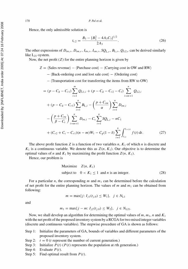
Hence, the only admissible solution is

tr,2 = B3 − {B23 − 4A3C3}1/2

2A3. (26)

The other expressions of Drw,r , Dow,r , Irw,r , Iow,r , SQL,r , BL,r , QL2,r can be derived similarlylike L21-system.

Now, the net profit (Z) for the entire planning horizon is given by

Z = 〈Sales revenue〉 − 〈Purchase cost〉 − 〈Carrying cost in OW and RW〉− 〈Back-ordering cost and lost sale cost〉 − 〈Ordering cost〉− 〈Transportation cost for transferring the items from RW to OW〉

= (p − Cd − Cr1)

m∑i=1

QL1,i + (p − Cd − Cr2 − Ct)

n∑i=m+1

QL2,i

+ (p − Cd − Cr1)

n∑i=1

BL,i −(

p + Cow

α

) n∑i=1

Dow,i

−(

p + Crw

β − Ct

) n∑i=m+1

Drw,i − Cs

n∑i=1

SQL,i − nC1

+ (Cr2 + Ct − Cr1)(n − m)W1 − Cp(1 − δ)

n∑i=1

∫ ti+1,0

ti,2

f (t) dt. (27)

The above profit function Z is a function of two variables n, K1 of which n is discrete andK1 is a continuous variable. We denote this as Z(n, K1). Our objective is to determine theoptimal values of n and K1 by maximizing the profit function Z(n, K1).

Hence, our problem is

Maximize Z(n, K1)

subject to 0 < K1 ≤ 1 and n is an integer. (28)

For a particular n, the corresponding m and m1 can be determined before the calculationof net profit for the entire planning horizon. The values of m and m1 can be obtained fromfollowing:

m = max{j : Ij1(tj,0) ≤ W1}, j ∈ NL1

and

m1 = max{j − m: Ij2(tj,0) ≤ W2}, j ∈ NL21.

Now, we shall develop an algorithm for determining the optimal values of m, m1, n and K1

with the net profit of the proposed inventory system by a RCGA for two mixed integer variables(discrete and continuous variables). The stepwise procedure of GA is shown as follows:

Step 1: Initialize the parameters of GA, bounds of variables and different parameters of theproposed inventory system.

Step 2: t = 0 (t represent the number of current generation.)Step 3: Initialize P(t) (P(t) represents the population at t th generation.)Step 4: Evaluate P(t).Step 5: Find optimal result from P(t).

Dow

nloa

ded

By:

[IN

FLIB

NE

T, In

dia

orde

r 200

5] A

t: 07

:24

16 F

ebru

ary

2008

GA mixed integer non-linear programming 171

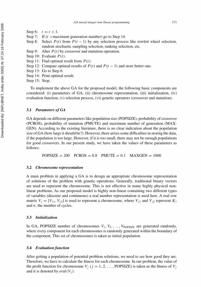
Step 6: t = t + 1.Step 7: If (t >maximum generation number) go to Step 14.Step 8: Select P(t) from P(t − 1) by any selection process like rowlett wheel selection,

random stochastic sampling selection, ranking selection, etc.Step 9: Alter P(t) by crossover and mutation operation.Step 10: Evaluate P(t).Step 11: Find optimal result from P(t).Step 12: Compare optimal results of P(t) and P(t − 1) and store better one.Step 13: Go to Step 6.Step 14: Print optimal result.Step 15: Stop.

To implement the above GA for the proposed model, the following basic components areconsidered: (i) parameters of GA, (ii) chromosome representation, (iii) initialization, (iv)evaluation function, (v) selection process, (vi) genetic operators (crossover and mutation).

3.1 Parameters of GA

GA depends on different parameters like population size (POPSIZE), probability of crossover(PCROS), probability of mutation (PMUTE) and maximum number of generation (MAX-GEN). According to the existing literature, there is no clear indication about the populationsize of GA (how large it should be?). However, there arises some difficulties in storing the data,if the population is too large. However, if it is too small, there may not be enough populationsfor good crossovers. In our present study, we have taken the values of these parameters asfollows:

POPSIZE = 200 PCROS = 0.8 PMUTE = 0.1 MAXGEN = 1000

3.2 Chromosome representation

A main problem in applying a GA is to design an appropriate chromosome representationof solutions of the problem with genetic operations. Generally, traditional binary vectorsare used to represent the chromosome. This is not effective in many highly physical non-linear problems. As our proposed model is highly non-linear containing two different typesof variables (discrete and continuous) a real number representation is used here. A real rowmatrix Vj = [Vj1, Vj2] is used to represent a chromosome, where Vj1 and Vj2 represent K1

and n, the number of cycles.

3.3 Initialization

In GA, POPSIZE number of chromosomes V1, V2, . . . , VPOPSIZE are generated randomly,where every component for each chromosomes is randomly generated within the boundary ofthe component. This set of chromosomes is taken as initial population.

3.4 Evaluation function

After getting a population of potential problem solutions, we need to see how good they are.Therefore, we have to calculate the fitness for each chromosome. In our problem, the value ofthe profit function for chromosome Vj (j = 1, 2, . . . , POPSIZE) is taken as the fitness of Vj

and it is denoted by eval (Vj ).

Dow

nloa

ded

By:

[IN

FLIB

NE

T, In

dia

orde

r 200

5] A

t: 07

:24

16 F

ebru

ary

2008

172 P. Pal et al.

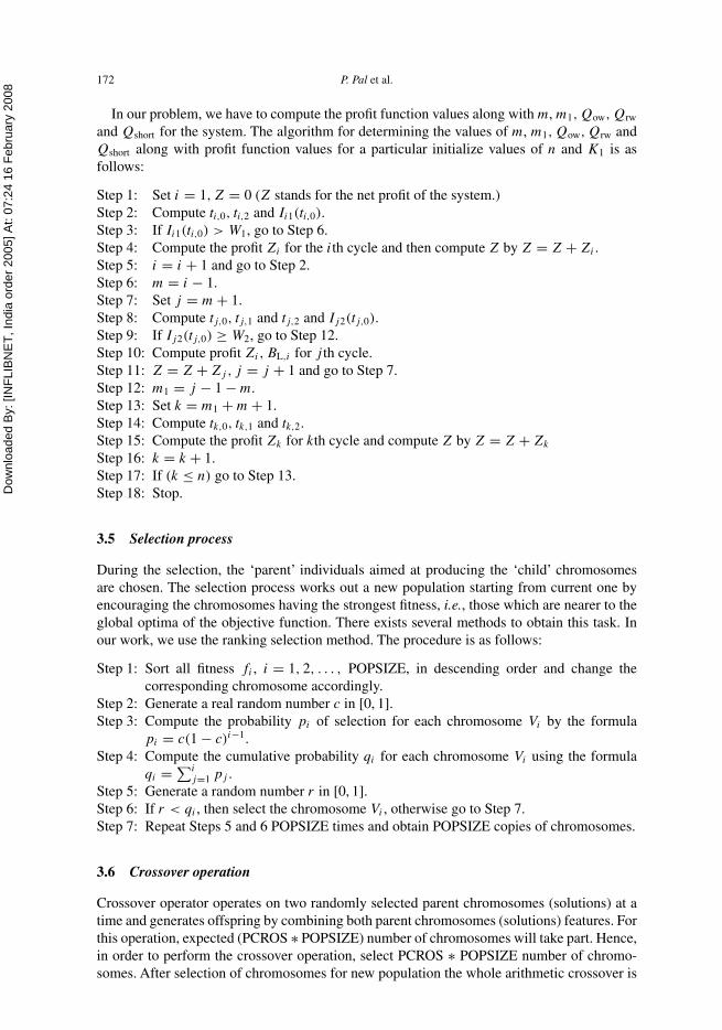
In our problem, we have to compute the profit function values along with m, m1, Qow, Qrw

and Qshort for the system. The algorithm for determining the values of m, m1, Qow, Qrw andQshort along with profit function values for a particular initialize values of n and K1 is asfollows:

Step 1: Set i = 1, Z = 0 (Z stands for the net profit of the system.)Step 2: Compute ti,0, ti,2 and Ii1(ti,0).Step 3: If Ii1(ti,0) > W1, go to Step 6.Step 4: Compute the profit Zi for the ith cycle and then compute Z by Z = Z + Zi .Step 5: i = i + 1 and go to Step 2.Step 6: m = i − 1.Step 7: Set j = m + 1.Step 8: Compute tj,0, tj,1 and tj,2 and Ij2(tj,0).Step 9: If Ij2(tj,0) ≥ W2, go to Step 12.Step 10: Compute profit Zi, BL,i for j th cycle.Step 11: Z = Z + Zj , j = j + 1 and go to Step 7.Step 12: m1 = j − 1 − m.Step 13: Set k = m1 + m + 1.Step 14: Compute tk,0, tk,1 and tk,2.Step 15: Compute the profit Zk for kth cycle and compute Z by Z = Z + Zk

Step 16: k = k + 1.Step 17: If (k ≤ n) go to Step 13.Step 18: Stop.

3.5 Selection process

During the selection, the ‘parent’ individuals aimed at producing the ‘child’ chromosomesare chosen. The selection process works out a new population starting from current one byencouraging the chromosomes having the strongest fitness, i.e., those which are nearer to theglobal optima of the objective function. There exists several methods to obtain this task. Inour work, we use the ranking selection method. The procedure is as follows:

Step 1: Sort all fitness fi , i = 1, 2, . . . , POPSIZE, in descending order and change thecorresponding chromosome accordingly.

Step 2: Generate a real random number c in [0, 1].Step 3: Compute the probability pi of selection for each chromosome Vi by the formula

pi = c(1 − c)i−1.Step 4: Compute the cumulative probability qi for each chromosome Vi using the formula

qi = ∑ij=1 pj .

Step 5: Generate a random number r in [0, 1].Step 6: If r < qi , then select the chromosome Vi , otherwise go to Step 7.Step 7: Repeat Steps 5 and 6 POPSIZE times and obtain POPSIZE copies of chromosomes.

3.6 Crossover operation

Crossover operator operates on two randomly selected parent chromosomes (solutions) at atime and generates offspring by combining both parent chromosomes (solutions) features. Forthis operation, expected (PCROS ∗ POPSIZE) number of chromosomes will take part. Hence,in order to perform the crossover operation, select PCROS ∗ POPSIZE number of chromo-somes. After selection of chromosomes for new population the whole arithmetic crossover is

Dow

nloa

ded

By:

[IN

FLIB

NE

T, In

dia

orde

r 200

5] A

t: 07

:24

16 F

ebru

ary

2008

GA mixed integer non-linear programming 173

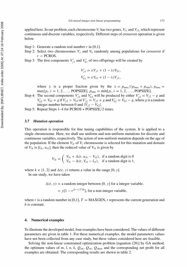
applied here. In our problem, each chromosome Vi has two genes, Vi1 and Vi2, which representcontinuous and discrete variables, respectively. Different steps of crossover operation is givenbelow.

Step 1: Generate a random real number r in [0,1].Step 2: Select two chromosomes Vj and Vk randomly among populations for crossover if

r < PCROS.Step 3: The first components V ′

j1 and V ′k1 of two offsprings will be created by

V ′j1 = λVj1 + (1 − λ)Vk1,

V ′k1 = λVk1 + (1 − λ)Vj1,

where λ is a proper fraction given by the λ = pmax/(pmax + pmin), pmax =max[pi, i = 1, 2, . . . , POPSIZE], pmin = min[pi, i = 1, 2, . . . , POPSIZE].

Step 4: The second components V ′j2 and V ′

k2 will be produced by either V ′j2 = Vj2 − g and

V ′k2 = Vk2 + g if Vj2 > Vk2 or V ′

j2 = Vj2 + g and V ′k2 = Vk2 − g, where g is a random

integer number between 0 and |Vj2 − Vk2|.Step 5: Repeat Steps 1–4 for PCROS ∗ POPSIZE/2 times.

3.7 Mutation operation

This operation is responsible for fine tuning capabilities of the system. It is applied to asingle chromosome. Here, we shall use uniform and non-uniform mutations for discrete andcontinuous variables, respectively. The action of non-uniform mutation depends on the age ofthe population. If the element Vik of Vi chromosome is selected for this mutation and domainof Vik is [lik, uik], then the reduced value of Vik is given by

Vik =(

Vik + �(t, uik − Vik), if a random digit is 0Vik − �(t, Vik − lik), if a random digit is 1,

where k ∈ {1, 2} and �(t, y) returns a value in the range [0, y].In our study, we have taken

�(t, y) = a random integer between [0, y] for a integer variable,

= y[1 − r(1−t/T )b], for a non-integer variable,

where r is a random number in [0,1], T = MAXGEN, t represents the current generation andb is constant.

4. Numerical examples

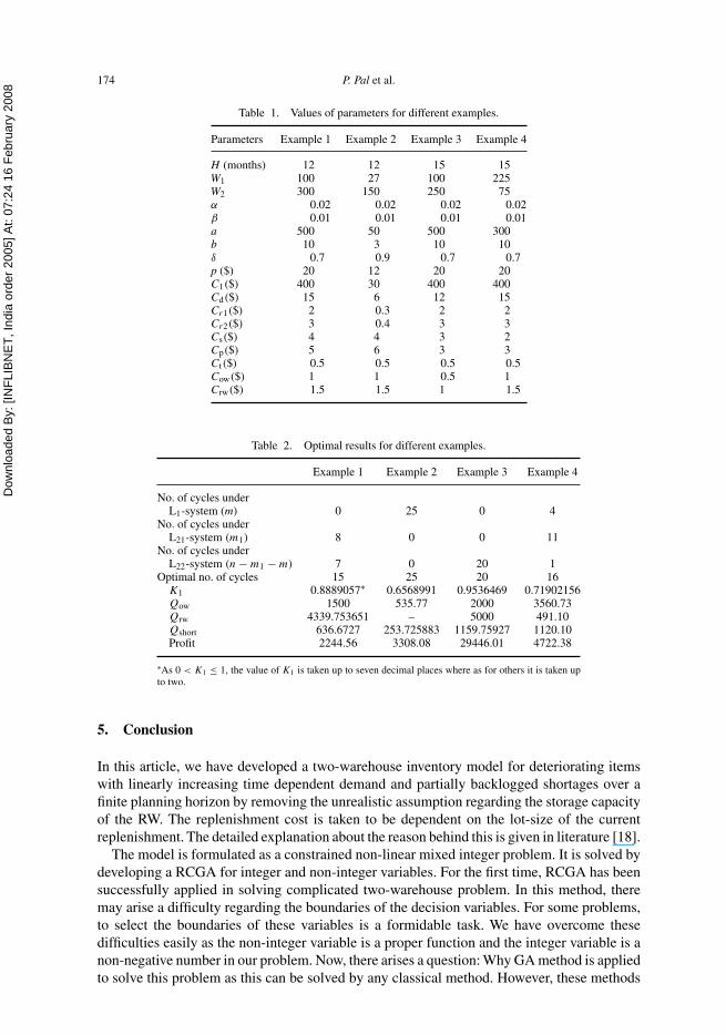
To illustrate the developed model, four examples have been considered. The values of differentparameters are given in table 1. For these numerical examples, the model parameters valueshave not been collected from any case study, but these values considered here are feasible.

Solving the non-linear constrained optimization problem [equation (28)] by GA method,the optimum values of m, l, n, k, Qow, Qrw, Qshort and the corresponding net profit for allexamples are obtained. The corresponding results are shown in table 2.

Dow

nloa

ded

By:

[IN

FLIB

NE

T, In

dia

orde

r 200

5] A

t: 07

:24

16 F

ebru

ary

2008

174 P. Pal et al.

Table 1. Values of parameters for different examples.

Parameters Example 1 Example 2 Example 3 Example 4

H (months) 12 12 15 15W1 100 27 100 225W2 300 150 250 75α 0.02 0.02 0.02 0.02β 0.01 0.01 0.01 0.01a 500 50 500 300b 10 3 10 10δ 0.7 0.9 0.7 0.7p ($) 20 12 20 20C1($) 400 30 400 400Cd($) 15 6 12 15Cr1($) 2 0.3 2 2Cr2($) 3 0.4 3 3Cs($) 4 4 3 2Cp($) 5 6 3 3Ct($) 0.5 0.5 0.5 0.5Cow($) 1 1 0.5 1Crw($) 1.5 1.5 1 1.5

Table 2. Optimal results for different examples.

Example 1 Example 2 Example 3 Example 4

No. of cycles underL1-system (m) 0 25 0 4

No. of cycles underL21-system (m1) 8 0 0 11

No. of cycles underL22-system (n − m1 − m) 7 0 20 1

Optimal no. of cycles 15 25 20 16K1 0.8889057∗ 0.6568991 0.9536469 0.71902156Qow 1500 535.77 2000 3560.73Qrw 4339.753651 – 5000 491.10Qshort 636.6727 253.725883 1159.75927 1120.10Profit 2244.56 3308.08 29446.01 4722.38

∗As 0 < K1 ≤ 1, the value of K1 is taken up to seven decimal places where as for others it is taken upto two.

5. Conclusion

In this article, we have developed a two-warehouse inventory model for deteriorating itemswith linearly increasing time dependent demand and partially backlogged shortages over afinite planning horizon by removing the unrealistic assumption regarding the storage capacityof the RW. The replenishment cost is taken to be dependent on the lot-size of the currentreplenishment. The detailed explanation about the reason behind this is given in literature [18].

The model is formulated as a constrained non-linear mixed integer problem. It is solved bydeveloping a RCGA for integer and non-integer variables. For the first time, RCGA has beensuccessfully applied in solving complicated two-warehouse problem. In this method, theremay arise a difficulty regarding the boundaries of the decision variables. For some problems,to select the boundaries of these variables is a formidable task. We have overcome thesedifficulties easily as the non-integer variable is a proper function and the integer variable is anon-negative number in our problem. Now, there arises a question: Why GA method is appliedto solve this problem as this can be solved by any classical method. However, these methods

Dow

nloa

ded

By:

[IN

FLIB

NE

T, In

dia

orde

r 200

5] A

t: 07

:24

16 F

ebru

ary

2008

GA mixed integer non-linear programming 175

do not guarantee about the solution status: whether the results give global or local optima? AsGA method is a stochastic search method, it always gives the global optima.

The present model is applicable for the product (e.g., food grains) whose production isperiodical and demand increases linearly with time.

Further extension of this model can be done considering some realistic situations, such asmulti-items and quantity discount policies. In addition, this model can be constructed withfuzzy/stochastic parameters, imprecise objective, etc.

Acknowledgements

The authors are grateful to the referee(s) for their helpful suggestion and comments in revisingthe paper to the present form.

References[1] Goldberg, D.E., 1989, Genetic Algorithms: Search, Optimization and Machine Learning (Reading, MA:

Addison Wesley).[2] Michalawicz, Z., 1992, Genetic Algorithms + Data structure = Evaluation Programs (Berlin: Springer Verlag).[3] Sakawa, M., 2002, Genetic Algorithms and Fuzzy Multiobjective Optimization (Kluwer Academic Publishers).[4] Choi, I.C., Kim, S.I. and Kim, H.S., 2003, A genetic algorithm with a mixed region search for the asymmetric

traveling salesman problem. Computer & Operations Research, 30, 773–786.[5] Davis, L., 1991, Handbook of Genetic Algorithms (New York: Van Nostrand Reinhold).[6] Bessaou, M. and Siarry, P., 2001, A genetic algorithm with real-value coding to optimize multimodal continuous

functions. Structural and Multidisciplinary Optimization, 23, 63–74.[7] Östermark, R., 2004, A multipurpose parallel genetic hybrid algorithm for non-linear non-convex programming

problems. European Journal of Operational Research, 152, 195–214.[8] Khouja, M., Michalawicz, Z. and Wilmot, M., 1998, The use of genetic algorithms to solve the economic lot

size scheduling problem. European Journal of Operational Research, 110, 509–524.[9] Sarkar, R. and Newton, C., 2002, A genetic algorithm for solving economic lot-size scheduling problem.

Computers and Industrial Engineering, 42, 189–198.[10] Mandal, S. and Maiti, M., 2002, Multi item fuzzy EOQ models using genetic algorithm. Computers and Industrial

Engineering, 44, 105–117.[11] Yokoyama, M. and Lewis III, H.W., 2003, Optimization of the stochastic dynamic production cycling problem

by a genetic algorithm. Computers of Operations Research, 30, 1831–1849.[12] Goswami, A. and Chaudhuri, K.S., 1992, An economic order quantity model for items with two levels of storage

for a linear trend in demand. Journal of the Operational Research Society, 43, 157–167.[13] Bhunia, A.K. and Maiti, M., 1994, A two-warehouse inventory model for a linear trend in demand. Opsearch,

31, 318–329.[14] Bhunia, A.K. and Maiti, M., 1997, A two warehouses inventory model for deteriorating items with a linear trend

in demand and shortages. Journal of the Operational Research Society, 49, 287–292.[15] Pakkala, T.P.M., and Achary, K.K., 1992, A deterministic inventory model for deteriorating items with two

warehouses and finite replenishment rate. European Journal of Operational Research, 57, 71–76.[16] Benkherouf, L.A., 1997, A deterministic order level inventory model for deteriorating items with two storage

facilities. International Journal of Production Economics, 48, 167–175.[17] Lee, C.C., and Ma, C.Y., 2000, Optimal inventory policy for deteriorating items with two warehouse and time

dependent demands. Production Planning Control, 7, 689–696.[18] Kar, S., Bhunia, A.K. and Maiti, M., 2001, Deterministic inventory model with two levels of storage, a linear

trend in demand and a fixed time horizon. Computers & Operations Research, 28, 1315–1331.[19] Goyal, S.K., Horiga, M.A. and Alyan, A., 1996, The trended inventory lot-sizing problem with shortages under

a new replenishment policy. Journal of the Operational Research Society, 47, 1286–1295.[20] Chakrabarti, T. and Chaudhuri, K.S., 1997, An EOQ model for deteriorating items with a linear trend in demand

and shortages in all cycles. International Journal of Production Economics, 49, 205–213.[21] Bhunia, A.K. and Maiti, M., 1999, An inventory model of deteriorating items with lot-size dependent

replenishment cost and a linear trend in demand. Applied Mathematical Modelling, 23, 301–308.