73

AMO-Advanced Modeling and Optimization, Volume 8, Number 1, 2006

An Application of real-coded Genetic Algorithm (RCGA) for integer linear

programming in Production-Transportation Problems with

flexible transportation cost

R. K. Guptaa

aDepartment of Business Administration, North Bengal University, Darjeeling – 734 430, India,

A. K. Bhuniab

bDepartment of Mathematics. University of Burdwan, Burdwan-713 104, India,

Abstract

In this paper, an application of real-coded Genetic Algorithm (RCGA) for integer linear programming

in a production-transportation problem has been discussed. In this discussion, firstly, the model has

been developed under the assumption that a company produces a single commodity in different

factories, situated at different places. The raw material cost, production cost as well as marketing

costs per unit are different for different factories. The transportation cost from a particular factory to a

particular market is not fixed, but flexible It depends upon the transported units and the capacity

of transport vehicle. Generally, when the number of transported units is above a certain limit, then

the transportation cost for full load of vehicle will be charged, otherwise transportation cost is charged

per unit. The mathematical formulation of the problem indicates that the model is an integer linear

programming problem. In order to solve the problem, a real coded genetic algorithm (RCGA) for

discrete values of decision variables with rank based selection, whole crossover and mutation has

been developed. The proposed model has been solved using RCGA and illustrated with four different

types of numerical examples.

Keywords : Production-Transportation problem; Linear Programming; Genetic Algorithm

AMS Mathematics Subject Classification : 90B06, 90B30.

bCorresponding Author : E-mail: bhuniaak@rediffmail.com

74

1. Introduction

Among the various forms of linear programming problem, a popular and important type is the

traditional transportation problem, in which the objective is to minimize the cost of transportation of

various amounts of a single homogeneous commodity from different sources to different destinations.

The subject was initiated by [Hitchock, 1941]. After Hitchcock, several researchers have developed

various methodologies for solving the transportation problem. Among them, the names of researchers

[Dantzig, 1963], [ Charnes, Copper, 1954] and others are worth-mentioning.

Generally, the traditional transportation problem (TP) is a minimization problem in which the

total transportation cost for transporting the goods from source to the destination is minimized.

However, due to the fierce competition resulting out of rapid changes of the Global economy and to

maintain the quality of the item as well as the goodwill of the company, some manufacturing

companies are forced to keep the following activities simultaneously under their own control:

1. Manufacturing and Marketing of the commodity.

2. Selling at different showrooms situated at different important markets / locations.

3. Transportation of commodities from different factories to different showrooms.

As a result, the overall objective of that manufacturing company is to maximize the profit of the

system according to the prescribed demands of different markets as well as the capacity of different

factories.

In the traditional transportation problem, it is assumed that the transportation cost (per unit)

for transferring the commodities from a particular source to a particular destination is fixed. However,

under real life situation when the number of transported units is above a certain limit, then one or

more transport vehicle is generally hired to transport those units from a particular source to a

particular destination, and this normally results in the lowering down of effective cost per unit. Also,

the factors like road conditions, weather, etc can affect the unit transportation cost.

A genetic algorithm (GA) is a computerized stochastic search and optimization method which

works by mimicking the evolutionary principles and chromosomal processing in natural genetics. It is

based on Darwin’s principles of “survival of the fittest”. It is executed iteratively on the set of real /

binary coded solution called population. Every solution is assigned a fitness, which is directly related

to the objective function of the search and optimization problem. There after, applying three operators

similar to natural genetic operators – selection / representation, crossover, and mutation, the

population of solutions is modified to a new population. GA works iteratively by successively

applying these three operators in each generation till a termination criterion is satisfied. The concept

of this algorithm was first conceived by Prof. J. H. Holland, University of Michigan, Ann Arbor in

1965. There after, a number of researchers have contributed to the development of this field. Detail

works on the development of the subject is evident in the books of [Goldberg, 1989], [Michalawicz,

75

1996], [Deb, 1995], [ Sakawa, 2002] and others.

In our present study, we have developed a realistic production-transportation model under the

assumption that a company is undergoing the following activities:

(i) Producing a single homogeneous product in different factories (situated in different

places with different raw material cost, production cost and marketing cost per unit).

(ii) Transporting the product to different show-rooms (with different selling prices per unit).

The unit transportation cost from a particular source to a particular destination is not

fixed, but flexible. Generally, when the number of transported units is above a certain

limit, then the transportation cost for full load of vehicle will be charged, otherwise

transportation cost is charged per unit.

(iii) Selling the product in different markets.

provided that objective of the company is to maximize the total profit.

In order to solve the problem for discrete values of decision variables, we have developed a real

coded genetic algorithm for discrete values of decision variables with rank based selection, crossover

and mutation. Finally the sensitivity of the solutions have been examined by

(i) Changing the cost.

(ii) Changing the selling prices.

(iii) Changing the capacity of the transport vehicle.

(iv) Making once the problem balanced and then unbalanced.

2. Assumptions and Notations :

The following assumptions and notations are used in developing the proposed model.

(i) A company has m factories iF (producing a homogeneous product) with capacity ai (i=

1,2,…,m) and there are n showrooms in markets jM with demand(requirement) bj

(j=1,2,…,n).

(ii) The transportation cost is constant for a transport vehicle of a given capacity (even if the

quantity shipped is less than the full load capacity of that transport vehicle by some quantity).

(iii) The capacity of a transport vehicle is K units.

(iv) xij represents the unknown quantity to be transported from the factory Fi to the market Mj.

(v) Cij be the transportation cost for a full load of transport vehicle and Cij/ be the transportation

cost per unit item from iF to jM .

(vi) Uij be the upper break point, some units less than K but more than Uij, the transportation cost

for the whole quantity is Cij.

76

Hence Uij = [ Cij / Cij/] < K where [ Cij / Cij

/] is the greatest integer value which is less

than or equal to Cij / Cij/.

(vii) riC and piC be the respective raw material and production costs per unit in the factory

iF ( 1,2,...., )i m= of the company.

(viii) jp be the selling price per unit in the market ( 1, 2,..., )jM j n= .

3. Model formulation of the problem

The Total Revenue TR of the company is given by

1 1

n m

j ijj i

TR p x= =

= ∑∑and the total production cost including the raw material cost is

( )m

ti1 1 i=1 j=1

= where m n n

ri pi ij ij ti ri pii j

C C x C x C C C= =

+ = +∑∑ ∑∑

Transportation cost

When the transported quantity from the i th factory to the j th show-room is greater than one integral

transport vehicle load, the transported quantity xij can be expressed as:

xij=nijK + kiqij where nij=0 or any finite integer, ki = 0 or 1 and qij<K. (1)

In this case, two situations may arise.

(i) nijK < xij ≤ nijK + Uij (ii) nijK + Uij <xij ≤ (nij+1)K (2)

Hence the transportation cost of xij units from the i th factory to the j th show-room is given by

TCij = nijCij + (xij – nijK).Cij/ where nijK< xij ≤ nij+Uij

= (nij + 1)Cij where nijK + Uij <xij ≤ (nij+1)K (3)

Now,the total profit of the company is given by

Z = <total revenue> - <production cost> - <row material cost> - <transportation cost>

Again, the supply and demand constraints are as follows:

1

, i = 1, 2,...,n

ij ij

x a m=

=∑ (4)

77

1

, j =1,2,...,nm

ij ji

x b=

=∑ (5)

Hence the problem of the company is

Max1 1 1 1 1 1

n m m n m n

ij j ti ij ijj i i j i j

Z x p C x TC= = = = = =

= − −∑∑ ∑∑ ∑∑ (6)

subject to the constraints

1

, i = 1, 2,...,n

ij ij

x a m=

=∑ (7)

and

1

, j =1,2,...,nm

ij ji

x b=

=∑ (8)

xij ≥ 0 and integers

In this situation , three cases may arise:

Case-I : 1 1

;m n

i ji j

a b= =

=∑ ∑ (9)(i)

Case-II : 1 1

;m n

i ji j

a b= =

>∑ ∑ (9)(ii)

Case-III: 1 1

;m n

i ji j

a b= =

<∑ ∑ (9)(iii)

In Case-I, the above problem is a balanced problem, whereas in Case-II & Case-III, it is

unbalanced. In Case-II, the total capacity of the source is greater than the total demand of the

destination. Where as in Case-III, the total capacity is less than the total demand.

4. Implementation of GA

Now, we shall develop a GA with real value coding for solving the above constrained

maximization problem involving m × n integer variables. The general working principle of GA is as

follows:

Step-1: Initialize the parameters of Genetic Algorithm and different parameters of the transportation

problem.

Step-2: t = 0 [ t represents the number of current generation.]

Step-3: Initialize P(t) [ P(t) represents the population at t-th generation]

Step-4: Evaluate P(t).

Step-5: Find best result from P(t).

Step-6: t = t+1.

78

Step-7: If (t > maximum generation number) go to step-14

Step-8: Select P(t) from P(t-1) by any selection process like rowlett wheel selection, tournament

selection, ranking selection etc.

Step-9: Alter P(t) by crossover and mutation operation.

Step-10: Evaluate P(t).

Step-11: Find best result from P(t).

Step-12: Compare best results of P(t) and P(t-1) and store the better one.

Step-13: Go to step-6.

Step-14: Print final best result.

Step-15: Stop.

For implementing the above GA in solving maximum problems developed in this model, the

following basic components are considered.

• Parameters of GA

• Representation of chromosomes.

• Initialization of chromosomes

• Evaluation of fitness function

• Selection process

• Genetic operators ( crossover and mutation)

Parameters of GA

Genetic Algorithm (GA) depends on some parameters like population size (POPSIZE), maximum

generation number (MAXGEN), probability of crossover (PCROS) and probability of mutation

(PMUTE). Although there is no clear indication about the population size of GA, some difficulties

may arise in storing of the data for larger population size. However, for small population size, the

crossover and mutation operations cannot be implemented accordingly. Again according to genetics, it

is obvious that the probability of crossover is always greater than that of mutation.. Generally, the

probabilities of crossover and mutation are taken as 0.75 to 0.9 and 0.05 to 0. 2 respectively. In our

present study, we have taken the values of those parameters as follows:

POPSIZE = 50, PCROS = 0.8, PMUTE = 0.05, MAXGEN = 700.

Initialization

Generally, each component (gene) of a chromosome of the population of GA is initialized randomly

within the boundary of the component, satisfying all the constraints given in the problem. However,

for the transportation problem, the initialization of any component of a chromosome cannot be done

by the said procedure, as the boundary of each component is not specified in the problem. For this

79

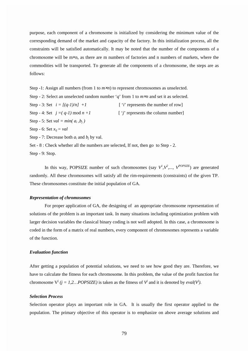
purpose, each component of a chromosome is initialized by considering the minimum value of the

corresponding demand of the market and capacity of the factory. In this initialization process, all the

constraints will be satisfied automatically. It may be noted that the number of the components of a

chromosome will be m×n, as there are m numbers of factories and n numbers of markets, where the

commodities will be transported. To generate all the components of a chromosome, the steps are as

follows:

Step -1: Assign all numbers (from 1 to m×n) to represent chromosomes as unselected.

Step - 2: Select an unselected random number ‘q’ from 1 to m×n and set it as selected.

Step - 3: Set i = [(q-1)/n] +1 [ ‘i’ represents the number of row]

Step - 4: Set j =( q-1) mod n +1 [ ‘j’ represents the column number]

Step - 5: Set val = min( ai ,bj )

Step - 6: Set xij = val

Step - 7: Decrease both ai and bj by val.

Set - 8 : Check whether all the numbers are selected, If not, then go to Step - 2.

Step - 9: Stop.

In this way, POPSIZE number of such chromosomes (say V1,V2,..., VPOPSIZE) are generated

randomly. All these chromosomes will satisfy all the rim-requirements (constraints) of the given TP.

These chromosomes constitute the initial population of GA.

Representation of chromosomes

For proper application of GA, the designing of an appropriate chromosome representation of

solutions of the problem is an important task. In many situations including optimization problem with

larger decision variables the classical binary coding is not well adopted. In this case, a chromosome is

coded in the form of a matrix of real numbers, every component of chromosomes represents a variable

of the function.

Evaluation function

After getting a population of potential solutions, we need to see how good they are. Therefore, we

have to calculate the fitness for each chromosome. In this problem, the value of the profit function for

chromosome Vj (j = 1,2…POPSIZE) is taken as the fitness of Vj and it is denoted by eval(Vj).

Selection Process

Selection operator plays an important role in GA. It is usually the first operator applied to the

population. The primary objective of this operator is to emphasize on above average solutions and

80

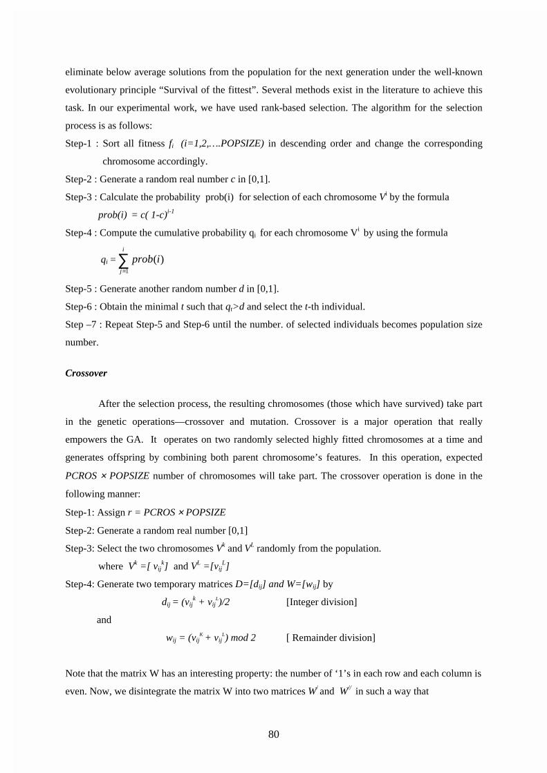
eliminate below average solutions from the population for the next generation under the well-known

evolutionary principle “Survival of the fittest”. Several methods exist in the literature to achieve this

task. In our experimental work, we have used rank-based selection. The algorithm for the selection

process is as follows:

Step-1 : Sort all fitness fi (i=1,2,….POPSIZE) in descending order and change the corresponding

chromosome accordingly.

Step-2 : Generate a random real number c in [0,1].

Step-3 : Calculate the probability prob(i) for selection of each chromosome Vi by the formula

prob(i) = c( 1-c)i-1

Step-4 : Compute the cumulative probability qi for each chromosome Vi by using the formula

qi =1

( )i

j

prob i=

∑Step-5 : Generate another random number d in [0,1].

Step-6 : Obtain the minimal t such that qt>d and select the t-th individual.

Step –7 : Repeat Step-5 and Step-6 until the number. of selected individuals becomes population size

number.

Crossover

After the selection process, the resulting chromosomes (those which have survived) take part

in the genetic operations—crossover and mutation. Crossover is a major operation that really

empowers the GA. It operates on two randomly selected highly fitted chromosomes at a time and

generates offspring by combining both parent chromosome’s features. In this operation, expected

PCROS × POPSIZE number of chromosomes will take part. The crossover operation is done in the

following manner:

Step-1: Assign r = PCROS × POPSIZE

Step-2: Generate a random real number [0,1]

Step-3: Select the two chromosomes Vk and VL randomly from the population.

where Vk =[ vijk] and VL =[vij

L]

Step-4: Generate two temporary matrices D=[dij] and W=[wij] by

dij = (vijk + vij

L)/2 [Integer division]

and

wij = (vijK

+ vijL) mod 2 [ Remainder division]

Note that the matrix W has an interesting property: the number of ‘1’s in each row and each column is

even. Now, we disintegrate the matrix W into two matrices W/ and W//

in such a way that

81

W= W/ +W//

and the number of ‘1’ s in each row and in each column of both W/ and W// is just half of the number

of ‘1’ s in each row and column of W. As a result, all the constraints will be satisfied automatically.

Step-5: Produce two offspring Y/ and Y// by

Y/= D + W/ and Y//=D + W//; where Y/ =[y/ij], Y//=[y//

ij],

W/=[w/ij] and W//=[w//

ij]

Step-6: Repeat Step - 2 and Step - 5 for r/2 times.

Mutation

Mutation introduces random variations into the population. It is applied to a single

chromosome only. It is usually performed with low probability. In a transportation problem, we shall

use a new type of mutation operation by selecting a sub matrix and finding all the rim-requirements of

the corresponding sub matrix of the original matrix of selected chromosome. Then by the

initialization process we assign the new values of the elements of the sub matrix such that all rim-

requirements of the corresponding sub matrix are satisfied. After that we replace the appropriate

elements of the matrix of a chromosome by the new elements from the sub matrix. In this way all the

constraints of the original problem have been satisfied.

5. Numerical Examples

The proposed model is illustrated for balanced and unbalanced cases considering four

different types of examples. For these numerical examples, the values of the parameters have not been

selected from any case study, but these values considered here are feasible. For each example, 20

independent runs have been performed from which the best value of the profit function along with the

corresponding values of the decision variables have been considered.

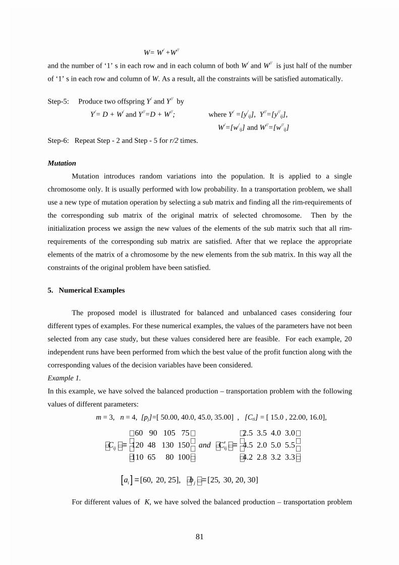
Example 1.

In this example, we have solved the balanced production – transportation problem with the following

values of different parameters:

m = 3, n = 4, [pj]=[ 50.00, 40.0, 45.0, 35.00] , [Cti] = [ 15.0 , 22.00, 16.0],

ij

60 90 105 75 2.5 3.5 4.0 3.0

120 48 130 150 C 4.5 2.0 5.0 5.5

110 65 80 100 4.2 2.8 3.2 3.3ijC and

′ = =

[ ] [60, 20, 25], [25, 30, 20, 30]i ja b = =

For different values of K, we have solved the balanced production – transportation problem

82

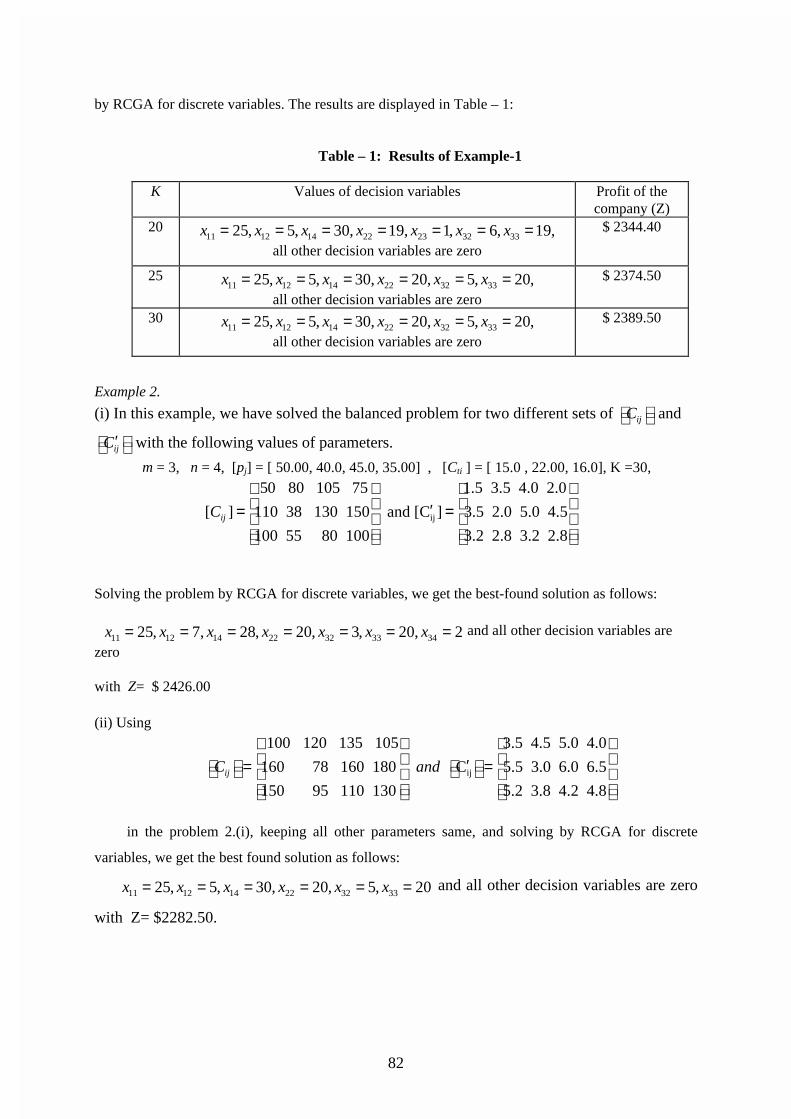
by RCGA for discrete variables. The results are displayed in Table – 1:

Table – 1: Results of Example-1

K Values of decision variables Profit of thecompany (Z)

2011 12 14 22 23 32 3325, 5, 30, 19, 1, 6, 19,x x x x x x x= = = = = = =

all other decision variables are zero

$ 2344.40

2511 12 14 22 32 3325, 5, 30, 20, 5, 20,x x x x x x= = = = = =

all other decision variables are zero

$ 2374.50

3011 12 14 22 32 3325, 5, 30, 20, 5, 20,x x x x x x= = = = = =

all other decision variables are zero

$ 2389.50

Example 2.

(i) In this example, we have solved the balanced problem for two different sets of ijC and

ijC′ with the following values of parameters.

m = 3, n = 4, [pj] = [ 50.00, 40.0, 45.0, 35.00] , [Cti ] = [ 15.0 , 22.00, 16.0], K =30,

ij

50 80 105 75 1.5 3.5 4.0 2.0

[ ] 110 38 130 150 and [C ] 3.5 2.0 5.0 4.5

100 55 80 100 3.2 2.8 3.2 2.8ijC

′= =

Solving the problem by RCGA for discrete variables, we get the best-found solution as follows:

11 12 14 22 32 33 3425, 7, 28, 20, 3, 20, 2x x x x x x x= = = = = = = and all other decision variables are

zero

with Z= $ 2426.00

(ii) Using

ij

100 120 135 105 3.5 4.5 5.0 4.0

160 78 160 180 C 5.5 3.0 6.0 6.5

150 95 110 130 5.2 3.8 4.2 4.8ijC and

′ = =

in the problem 2.(i), keeping all other parameters same, and solving by RCGA for discrete

variables, we get the best found solution as follows:

11 12 14 22 32 3325, 5, 30, 20, 5, 20x x x x x x= = = = = = and all other decision variables are zero

with Z= $2282.50.

83

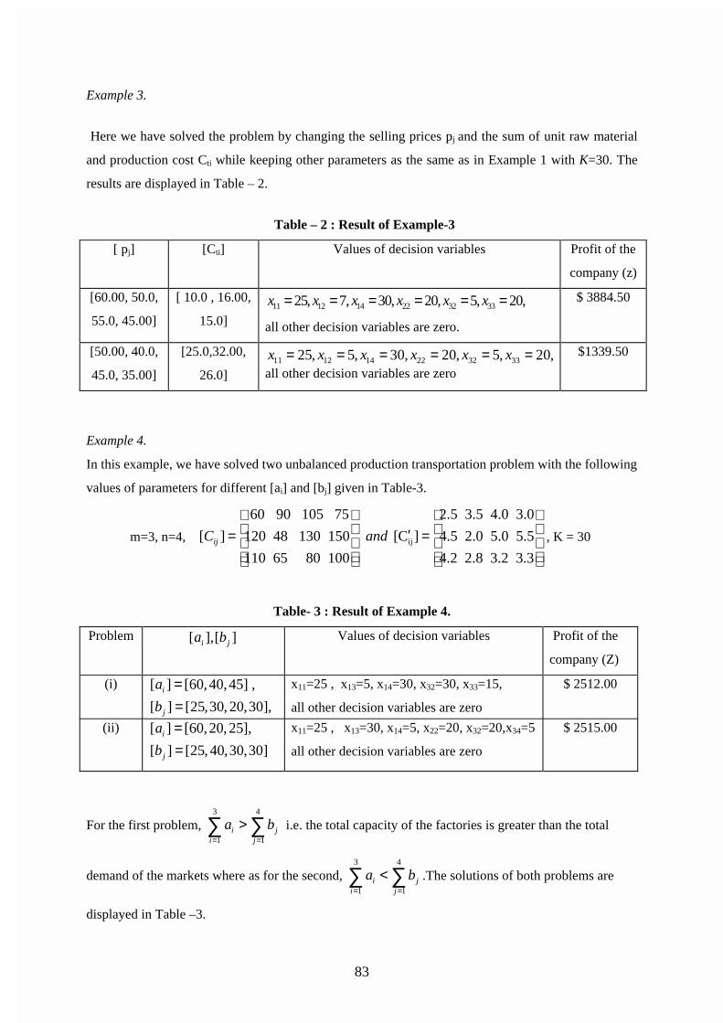
Example 3.

Here we have solved the problem by changing the selling prices pj and the sum of unit raw material

and production cost Cti while keeping other parameters as the same as in Example 1 with K=30. The

results are displayed in Table – 2.

Table – 2 : Result of Example-3

[ pj] [Cti] Values of decision variables Profit of the

company (z)

[60.00, 50.0,

55.0, 45.00]

[ 10.0 , 16.00,

15.0]11 12 14 22 32 3325, 7, 30, 20, 5, 20,x x x x x x= = = = = =

all other decision variables are zero.

$ 3884.50

[50.00, 40.0,

45.0, 35.00]

[25.0,32.00,

26.0]11 12 14 22 32 3325, 5, 30, 20, 5, 20,x x x x x x= = = = = =

all other decision variables are zero

$1339.50

Example 4.

In this example, we have solved two unbalanced production transportation problem with the following

values of parameters for different [ai] and [bj] given in Table-3.

m=3, n=4, ij

60 90 105 75 2.5 3.5 4.0 3.0

[ ] 120 48 130 150 [C ] 4.5 2.0 5.0 5.5

110 65 80 100 4.2 2.8 3.2 3.3ijC and

′= =

, K = 30

Table- 3 : Result of Example 4.

Problem [ ],[ ]i ja b Values of decision variables Profit of the

company (Z)

(i) [ ] [60,40,45] ,

[ ] [25,30, 20,30], i

j

a

b

==

x11=25 , x13=5, x14=30, x32=30, x33=15,

all other decision variables are zero

$ 2512.00

(ii) [ ] [60,20, 25],

[ ] [25, 40,30,30]i

j

a

b

==

x11=25 , x13=30, x14=5, x22=20, x32=20,x34=5

all other decision variables are zero

$ 2515.00

For the first problem, 3 4

1 1i j

i j

a b= =

>∑ ∑ i.e. the total capacity of the factories is greater than the total

demand of the markets where as for the second, 3 4

1 1i j

i j

a b= =

<∑ ∑ .The solutions of both problems are

displayed in Table –3.

84

Table-1 reveals that the profit of the company increases (as expected) with the increase of K

when all other parameters remain unaltered. From the solutions obtained from example 2, it is

observed that with the increment of costs [C] and [C/], the value of the profit of the company

decreases.(as expected). After taking a glance at Table-2, one can conclude that the profit increases

with the increase of each element of [pj] and decrease of [Cti]. Whereas the profit decreases with the

increase of each element of [Cti]

Concluding Remarks

In this paper, we have formulated and solved a production-transportation problem with the

flexible transportation cost for transferring commodities from a particular factory to a particular

show-room. For this purpose, a real coded GA (RCGA) for discrete variables with rank based

selection, whole crossover (applied for all genes of a chromosome) and a new type of mutation has

been developed.

In real-life situation, transportation costs of goods are fixed for a finite capacity of a transport

mode such as a truck, matador, etc. A fixed cost is charged against a certain amount of quantities

(upper ceiling) or more when a truck is deployed whether it is utilized fully or partially. For the

quantities less than that upper ceiling, a uniform rate per unit is charged. In this paper, we have

considered the transportation cost explicitly considering the realistic situation.

The proposed production inventory problem is a constrained linear integer problem. To solve

this problem, a real-coded GA for integer variables has been developed. However, in GA, there may

arise a difficulty regarding the boundaries of the decision variables. In application problems, the

selection of boundaries of the decision variables is a formidable task. We have overcome these

difficulties by selecting the decision variables randomly and taking the minimum value of the

corresponding capacity and requirement of the source and destination respectively. In this process, all

constraints are satisfied automatically.

Also, in mutation operation, all the constraints have been satisfied automatically. However, in

crossover operation, special effort has been applied into the disintegration of W as a sum of W/ and

W// to satisfy the constraints automatically.

The model can be improved in different ways. One obvious area for future work would be to

perform similar analysis for the interval valued / fixed charge / non-linear transportation cost. Another

interesting research can be done by performing similar analysis for multi-objective transportation

problems.

References

[1] Arsham, H., (1992) Post optimality analysis of the transportaton problem. Journal of the

85

Operational Research Society , vol.43, pp. 121 – 139.

[2] Arshmam H, Khen AB.( 1989) A simplex type algorithm for general transportation problems :

an alternative to stepping-stone. Journal of the Operational Research Society; vol.40, pp.581-590.

[3] Charness A, Copper WW.( 1954) The steping stone method for explaining linear Programming

calculation in transportation problem. Management Science; vol. 1 pp. 49 - 69.

[4] Dantzig, GB.( 1963) Linear programming and extentions. Princeton , NJ; Prinston University

Press.

[5] Davis L.( 1991) Handbook of Genetic Algorithms. Van Nostrand Reinhold, Newyork.

[6] Deb K. (1995) Optimization for Engineering Design-Algorithms and Examples. Prentice Hall of

India,New Delhi .

[7] Forest S. (1993). Proceedings of 5-th international conference on Genetic Algorithms. Margen

Kaufmann, California.

[8] Goldberg DE (1989) Genetic Algorithms: Search, Optimization and Machine Learning. Addison

Wesley.

[9] Hitchock FL.(1941) The distribution of a product from several sources to numerous locations.

Journal of Mathematical Physics,vol 20, pp. 224-30.

[10] Holland JH. (1975)Adaptation of Natural and Artificial system, University of Michigan Press,

Ann Arbor,.

[11] Liu S T.( 2003) The total cost bounds of the transportation problem with varying demand and

supply. Omega , vol. 31, pp. 247 – 51.

[12] Michalawicz Z. (1996) Genetic Algorithms + Data structure= Evaluation Programs. Springer

Verlog, Berlin.

[13] Sakawa M. (2002) Genetic Algorithms and fuzzy multiobjective optimisation. Kluwer Academic

Publishers,

86

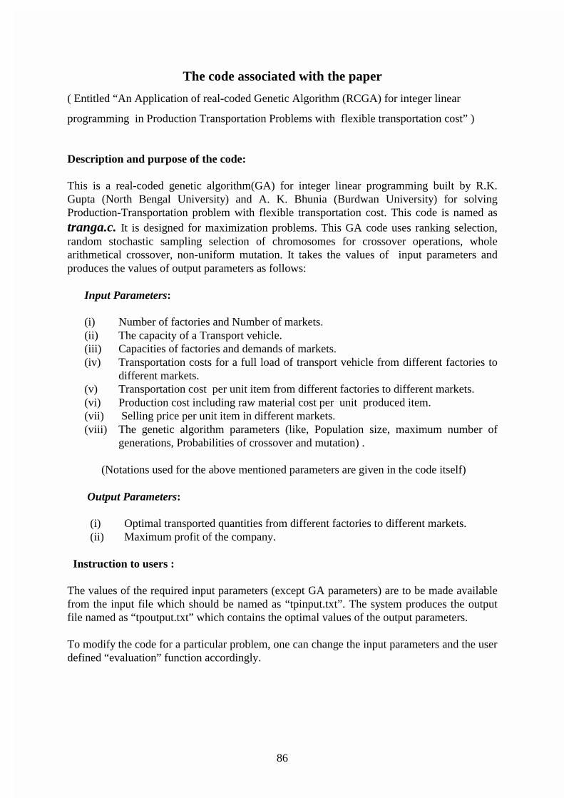
The code associated with the paper

( Entitled “An Application of real-coded Genetic Algorithm (RCGA) for integer linear

programming in Production Transportation Problems with flexible transportation cost” )

Description and purpose of the code:

This is a real-coded genetic algorithm(GA) for integer linear programming built by R.K.Gupta (North Bengal University) and A. K. Bhunia (Burdwan University) for solvingProduction-Transportation problem with flexible transportation cost. This code is named astranga.c. It is designed for maximization problems. This GA code uses ranking selection,random stochastic sampling selection of chromosomes for crossover operations, wholearithmetical crossover, non-uniform mutation. It takes the values of input parameters andproduces the values of output parameters as follows:

Input Parameters:

(i) Number of factories and Number of markets.(ii) The capacity of a Transport vehicle.(iii) Capacities of factories and demands of markets.(iv) Transportation costs for a full load of transport vehicle from different factories to

different markets.(v) Transportation cost per unit item from different factories to different markets.(vi) Production cost including raw material cost per unit produced item.(vii) Selling price per unit item in different markets.(viii) The genetic algorithm parameters (like, Population size, maximum number of

generations, Probabilities of crossover and mutation) .

(Notations used for the above mentioned parameters are given in the code itself)

Output Parameters:

(i) Optimal transported quantities from different factories to different markets.(ii) Maximum profit of the company.

Instruction to users :

The values of the required input parameters (except GA parameters) are to be made availablefrom the input file which should be named as “tpinput.txt”. The system produces the outputfile named as “tpoutput.txt” which contains the optimal values of the output parameters.

To modify the code for a particular problem, one can change the input parameters and the userdefined “evaluation” function accordingly.

87

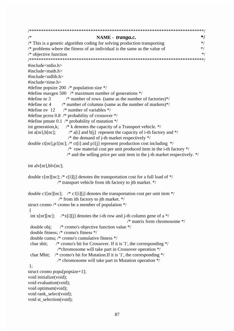
/**************************************************************************//* NAME - tranga.c. *//* This is a genetic algorithm coding for solving production transporting *//* problems where the fitness of an individual is the same as the value of *//* objective function *//**************************************************************************/#include<stdio.h>#include<math.h>#include<stdlib.h>#include<time.h>#define popsize 200 /* population size */#define maxgen 500 /* maximum number of generations */#define nr 3 /* number of rows (same as the number of factories)*/#define nc 4 /* number of columns (same as the number of markets)*/#define nv 12 /* number of variables */#define pcros 0.8 /* probability of crossover */#define pmute 0.1 /* probability of mutation */int generation,k; /* k denotes the capacity of a Transport vehicle. */int a[nr],b[nc]; /* a[i] and b[j] repesent the capacity of i-th factory and */

/* the demand of j-th market respectively */double ct[nr],p1[nc]; /* ct[i] and p1[j] represent production cost including */ /* raw material cost per unit produced item in the i-th factory */ /* and the selling price per unit item in the j-th market respectively. */

int alv[nr],blv[nc];

double c[nr][nc]; /* c[i][j] denotes the transportation cost for a full load of */ /* transport vehicle from ith factory to jth market. */

double c1[nr][nc]; /* c1[i][j] denotes the transportation cost per unit item */ /* from ith factory to jth market. */

struct cromo /* cromo be a member of population */ { int x[nr][nc]; /*x[i][j] denotes the i-th row and j-th column gene of a */

/* matrix form chromosome */ double obj; /* cromo's objective function value */ double fitness; /* cromo's fitness */ double cumu; /* cromo's cumulative fitness */ char sbit; /* cromo's bit for Crossover. If it is '1', the corresponding */

/*chromosome will take part in Crossover operation */ char Mbit; /* cromo's bit for Mutation.If it is '1', the corresponding */

/* chromosome will take part in Mutation operation */ };struct cromo popu[popsize+1];void initialize(void);void evaluation(void);void optimum(void);void rank_select(void);void st_selection(void);

88

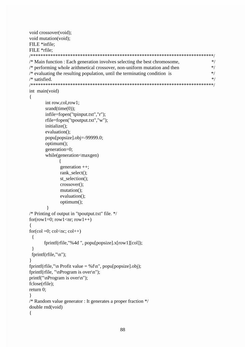
void crossover(void);void mutation(void);FILE *infile;FILE *rfile;/**************************************************************************//* Main function : Each generation involves selecting the best chromosome, *//* performing whole arithmetical crossover, non-uniform mutation and then *//* evaluating the resulting population, until the terminating condition is *//* satisfied. *//**************************************************************************/int main(void){

int row,col,row1; srand(time(0)); infile=fopen("tpinput.txt","r"); rfile=fopen("tpoutput.txt","w"); initialize(); evaluation(); popu[popsize].obj=-99999.0; optimum(); generation=0; while(generation<maxgen)

{ generation ++; rank_select(); st_selection(); crossover(); mutation(); evaluation(); optimum();

}/* Printing of output in "tpoutput.txt" file. */for(row1=0; row1<nr; row1++){for(col =0; col<nc; col++) {

fprintf(rfile,"%4d ", popu[popsize].x[row1][col]); } fprintf(rfile,"\n");}fprintf(rfile,"\n Profit value = %f\n", popu[popsize].obj);fprintf(rfile, "\nProgram is over\n");printf("\nProgram is over\n");fclose(rfile);return 0;}/* Random value generator : It generates a proper fraction */double rnd(void){

89

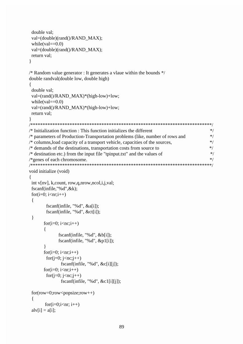
double val; val=(double)(rand()/RAND_MAX); while(val==0.0) val=(double)(rand()/RAND_MAX); return val;}

/* Random value generator : It generates a vlaue within the bounds */double randval(double low, double high){ double val; val=(rand()/RAND_MAX)*(high-low)+low; while(val==0.0) val=(rand()/RAND_MAX)*(high-low)+low; return val;}/**************************************************************************//* Initialization function : This function initializes the different *//* parameters of Production-Transportation problems (like, number of rows and *//* columns,load capacity of a transport vehicle, capacities of the sources, *//* demands of the destinations, transportation costs from source to *//* destination etc.) from the input file "tpinput.txt" and the values of *//*genes of each chromosome. *//**************************************************************************/void initialize (void){ int v[nv], k,count, row,q,nrow,ncol,i,j,val; fscanf(infile,"%d",&k); for(i=0; i<nr;i++) {

fscanf(infile, "%d", &a[i]); fscanf(infile, "%d", &ct[i]);

}for(i=0; i<nc;i++){

fscanf(infile, "%d", &b[i]);fscanf(infile, "%d", &p1[i]);

}for(i=0; i<nr;i++) for(j=0; j<nc;j++)

fscanf(infile, "%d", &c[i][j]);for(i=0; i<nr;i++) for(j=0; j<nc;j++)

fscanf(infile, "%d", &c1[i][j]);

for(row=0;row<popsize;row++) {

for(i=0;i<nr; i++) alv[i] = a[i];

90

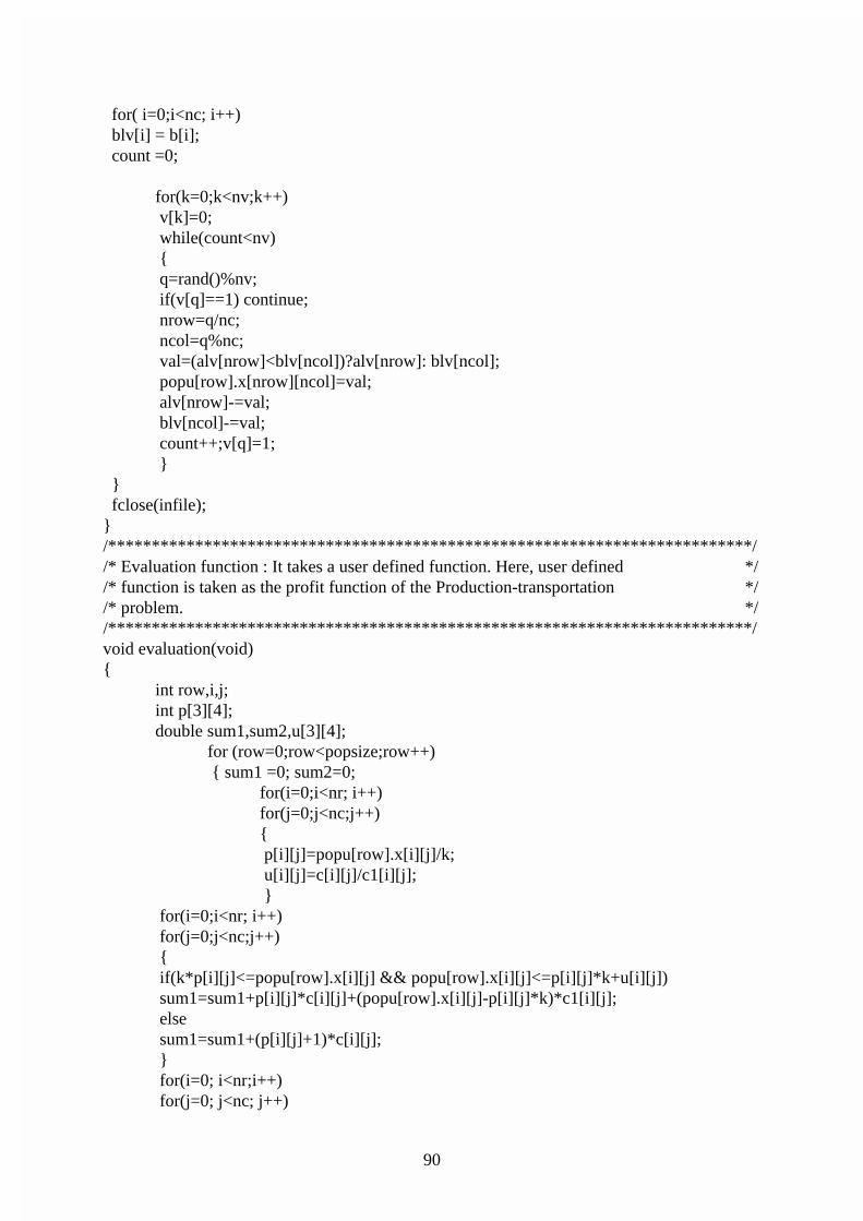
for( i=0;i<nc; i++) blv[i] = b[i]; count =0;

for(k=0;k<nv;k++) v[k]=0; while(count<nv) { q=rand()%nv; if(v[q]==1) continue; nrow=q/nc; ncol=q%nc; val=(alv[nrow]<blv[ncol])?alv[nrow]: blv[ncol]; popu[row].x[nrow][ncol]=val; alv[nrow]-=val; blv[ncol]-=val; count++;v[q]=1; }

} fclose(infile);}/**************************************************************************//* Evaluation function : It takes a user defined function. Here, user defined *//* function is taken as the profit function of the Production-transportation *//* problem. *//**************************************************************************/void evaluation(void){

int row,i,j;int p[3][4];double sum1,sum2,u[3][4];

for (row=0;row<popsize;row++) { sum1 =0; sum2=0;

for(i=0;i<nr; i++)for(j=0;j<nc;j++){ p[i][j]=popu[row].x[i][j]/k; u[i][j]=c[i][j]/c1[i][j]; }

for(i=0;i<nr; i++) for(j=0;j<nc;j++) { if(k*p[i][j]<=popu[row].x[i][j] && popu[row].x[i][j]<=p[i][j]*k+u[i][j]) sum1=sum1+p[i][j]*c[i][j]+(popu[row].x[i][j]-p[i][j]*k)*c1[i][j]; else sum1=sum1+(p[i][j]+1)*c[i][j]; } for(i=0; i<nr;i++) for(j=0; j<nc; j++)

91

sum2= sum2+(p1[j]-ct[i])*popu[row].x[i][j]; popu[row].obj=sum2-sum1;

} }

/**************************************************************************//* Optimum function : This function keeps track of the best member of the *//* population. Note that the last entry in the array population holds a *//* copy of the best individual. *//**************************************************************************/ void optimum(void) { int row,row1,idx,col; double max=-999999.0;

for(row=0;row<popsize;row++) if(max<popu[row].obj)

{max=popu[row].obj;idx=row;

}

/* If the best chromosome in current generation is available with respect */ /* to the earlier generation, then copy the same in the last entry of array */ /* population. */ if(max>popu[popsize].obj)

{popu[popsize].obj=popu[idx].obj;

for(row1=0; row1<nr; row1++)for(col=0;col<nc;col++) popu[popsize].x[row1][col]=popu[idx].x[row1][col];

} }

/**************************************************************************/ /* Selection function : Rank-based selection has been used in this function *//**************************************************************************/ void rank_select() {

struct rank {

int x1[nr][nc];double objec;double fit;

92

double cum; };struct rank popud[popsize];int row,col,i,j,them[nr][nc],i1;double r,them1,pp;for(row=0;row<popsize;row++)

{ for(i=0;i<nr;i++) for(j=0;j<nc;j++)

popud[row].x1[i][j]=popu[row].x[i][j]; popud[row].objec=popu[row].obj;

}for(row=0;row<popsize-1;row++)for(col=row+1;col<popsize;col++) {

if(popud[row].objec<popud[col].objec){ them1=popud[row].objec; popud[row].objec=popud[col].objec; popud[col].objec=them1; for(i=0;i<nr;i++) for(j=0;j<nc;j++)

{ them[i][j]=popud[row].x1[i][j]; popud[row].x1[i][j]=popud[col].x1[i][j]; popud[col].x1[i][j]=them[i][j];}

} }pp=rnd();for(row=0;row<popsize;row++)popud[row].fit=pp*pow((1-pp),row);popud[0].cum=popud[0].fit;for(row=1;row<popsize;row++)popud[row].cum=popud[row-1].cum+popud[row].fit;for(row=0;row<popsize;row++) {

i=0; r=rnd(); do

{ if(r<=popud[i].cum)

{ for(i1=0;i1<nr;i1++) for(j=0;j<nc;j++)

popu[row].x[i1][j]=popud[i].x1[i1][j]; popu[row].obj=popud[i].objec; break; }

93

elsei=i+1;

}while(i<popsize); }

}

/**************************************************************************/ /* Crossover selection : It selects the chromosomes which will take */ /* part in the crossover operation. For this purpose,Random stochastic */ /* Sampling function is used. */ /************************************************************************* / void st_selection(void) {

int row,Npointer,Pointer,esp,scale_change, count=0;double Dst,CDst,minft,sum=0.0;minft=popu[0].obj;for(row=1;row<popsize;row++) {

if(minft>popu[row].obj) minft=popu[row].obj;

}if(minft < 0)

scale_change=abs(int (minft))+1;for(row=0;row<popsize;row++)

sum=sum+popu[row].obj;if(minft < 0)

sum=sum+scale_change*popsize;for(row=0;row<popsize;row++)

if(minft < 0) popu[row].fitness =(popu[row].obj+scale_change)/sum;else popu[row].fitness =popu[row].obj/sum;

popu[0].cumu=popu[0].fitness; for(row=1;row<popsize;row++)

popu[row].cumu=popu[row-1].cumu+popu[row].fitness; Npointer=int(pcros*popsize); Dst=1.0/Npointer; for(row=0;row<popsize;row++)

popu[row].sbit='0'; para1: CDst=randval(0,Dst);

row=0; para2: for(Pointer=1;Pointer<=Npointer;Pointer++) {

while(CDst>=popu[row].cumu && popu[row].sbit == '1'){row=row+1;if(row>popsize) goto para1;}

popu[row].sbit='1';

94

count++; if(count == Npointer) break;

CDst=CDst+Dst; }if(count < Npointer) goto para2; }

/**************************************************************************/ /* Crossover function : This function takes two selected parents at a time */ /* and produces two offspring by whole arithmetical crossover. In that case, */ /* some of the offspring may be infeasible. To overcome it, a pepair algorithm */ /* is applied. *//**************************************************************************/ void crossover(void) {

double c1,maxft,minft;int m100, m101,row,row1,col,count,index[2], count1=0,count2=0,div[nr][nc];int rem[nr][nc], rem1[nr][nc], rem2[nr][nc];int i,j,n,k,c=0, Arem1rt[nr],rem1rt[nr],rt[nr];maxft=popu[0].fitness; /* maxfit means maximum of fitness */minft=popu[0].fitness; /* minfit means minimum of fitness */for(row=1;row<popsize;row++){ if(maxft<popu[row].fitness) maxft=popu[row].fitness; if(minft>popu[row].fitness) minft=popu[row].fitness;}c1=maxft/(maxft+minft);count=0; for(row=0;row<popsize;row++) if(popu[row].sbit=='1') {

index[count]=row; count=count+1; if(count==2) {

count=0; for(row1=0;row1<nr;row1++) for(col=0;col<nc;col++) { m100=popu[index[0]].x[row1][col]; m101=popu[index[1]].x[row1][col]; div[row1][col]=(m100+m101)/2; rem[row1][col]=(m100+m101)%2; } for(i=0;i<nr;i++)

{ rt[i]=0; for(j=0;j<nc;j++)

95

{ rt[i]= rt[i] + rem[i][j] ;} rem1rt[i]=(rt[i])/2;

} for(j=0;j<nc;j++) {

for(i=0;i<nr;i++) { if(rem[i][j]==0)

rem1[i][j]=0;if(rem[i][j]==1) { if(c%2==0) rem1[i][j]=1; else rem1[i][j]=0; c++; }

} }

for(i=0;i<nr;i++) { Arem1rt[i]=0;

for(j=0;j<nc;j++){ Arem1rt[i]=Arem1rt[i]+ rem1[i][j];}

}

for(i=0;i<nr;i++){ if(Arem1rt[i]>rem1rt[i]) {

for(k=0;k<nc;k++){ if(rem1[i][k]==1 && Arem1rt[i]>rem1rt[i]) {

for(n=0;n<nr;n++){ if(rem1[n][k]==0 && rem[n][k] !=0) if(Arem1rt[n]<rem1rt[n]) {

rem1[n][k]=1; rem1[i][k]=0;Arem1rt[n]=Arem1rt[n]+1;Arem1rt[i]=Arem1rt[i]-1;goto bb;

}}

} bb: ;}

96

}}

for(i=0;i<nr;i++)for(j=0;j<nc;j++) { rem2[i][j]=rem[i][j]-rem1[i][j]; } for(row1=0; row1<nr; row1++) for(col=0; col<nc; col++) { popu[index[0]].x[row1][col]=div[row1][col]+rem1[row1][col]; popu[index[1]].x[row1][col]=div[row1][col]+rem2[row1][col]; }

} }}/**************************************************************************//* Mutation function : Here, non-uniform mutation is applied to change the *//* selected gene from a selected chromosome of the population *//**************************************************************************/void mutation(void){

double r1;int i,j,k,q,v[nv],nrow,ncol,cou10,cou11;int row,col,n_mute,count=0, row1,val,count1,ccount, wnv;int rselect,cselect,r[nr],c[nc],w[nr][nc],sourcew[nr],destw[nc];for(row=0;row<popsize;row++)

popu[row].Mbit='0';n_mute = int(popsize*pmute);while(count < n_mute)

{ row = rand() % popsize; if(popu[row].Mbit =='0')

{ popu[row].Mbit ='1'; count++;}

}for(row=0;row<popsize;row++)if(popu[row].Mbit=='1') {

rselect=rand()%(nr-2)+2;cselect=rand()%(nc-2)+2;for(k=0;k<rselect;k++)

v[k]=0;cou10=0;while(cou10<rselect) {

q=rand()%nr;

97

if(v[q]==1) continue;r[cou10++]=q;v[q]=1;

}

for(k=0;k<cselect;k++)v[k]=0;cou11=0;while(cou11<cselect) {

q=rand()%nc;if(v[q]==1) continue;c[cou11++]=q;v[q]=1;

}

for(i=0; i<rselect; i++)for(j=0; j<cselect; j++)

w[i][j]=popu[row].x[r[i]][c[j]];for(i=0; i<rselect; i++)

{ sourcew[i]=0; for(j=0; j<cselect; j++)

sourcew[i]+=w[i][j];}

for(j=0; j<cselect; j++) {

destw[j]=0;for(i=0; i<rselect; i++)

destw[j]+=w[i][j]; }wnv = rselect*cselect;for(k=0;k<wnv;k++)

v[k]=0;count1 =0;

while(count1<wnv) { q=rand()%wnv; if(v[q]==1) continue; nrow=q/cselect; ncol=q%cselect; val=(sourcew[nrow]<destw[ncol])?sourcew[nrow]: destw[ncol]; w[nrow][ncol]=val; sourcew[nrow]-=val; destw[ncol]-=val; count1++;v[q]=1; }

for(i=0; i<rselect; i++)

98

{ for(j=0; j<cselect; j++){ popu[row].x[r[i]][c[j]]=w[i][j];

}}}}

----ooooOoooo----