Ages and magnetic structures of the South China Sea constrained by deep tow magnetic surveys and...

RESEARCH ARTICLE10.1002/2014GC005567

Ages and magnetic structures of the South China Seaconstrained by deep tow magnetic surveys and IODPExpedition 349Chun-Feng Li1, Xing Xu2, Jian Lin3, Zhen Sun4, Jian Zhu3, Yongjian Yao2, Xixi Zhao1, Qingsong Liu5,Denise K. Kulhanek6, Jian Wang1, Taoran Song1, Junfeng Zhao4, Ning Qiu4, Yongxian Guan2,Zhiyuan Zhou1, Trevor Williams7, Rui Bao8, Anne Briais9, Elizabeth A. Brown10, Yifeng Chen11,Peter D. Clift12, Frederick S. Colwell13, Kelsie A. Dadd14, Weiwei Ding15, Iv�an Hern�andez Almeida16,Xiao-Long Huang17, Sangmin Hyun18, Tao Jiang19, Anthony A. P. Koppers13, Qianyu Li20,Chuanlian Liu20, Zhifei Liu1, Renata H. Nagai21, Alyssa Peleo-Alampay22, Xin Su23,Maria Luisa G. Tejada24, Hai Son Trinh25, Yi-Ching Yeh26, Chuanlun Zhang20, Fan Zhang3,and Guo-Liang Zhang27

1State Key Laboratory of Marine Geology, Tongji University, Shanghai, China, 2Guangzhou Marine Geological Survey,Guangzhou, China, 3Department of Geology and Geophysics, Woods Hole Oceanographic Institution, Woods Hole, Massa-chusetts, USA, 4South China Sea Institute of Oceanology, CAS, Guangzhou, China, 5State Key Laboratory of LithosphericEvolution, Institute of Geology and Geophysics, CAS, Beijing, China, 6International Ocean Discovery Program, Texas A&MUniversity, College Station, Texas, USA, 7Lamont-Doherty Earth Observatory, Columbia University, Palisades, New York,USA, 8Geologisches Institut, Swiss Federal Institute of Technology, Z€urich, Switzerland, 9G�eosciences Environnement Tou-louse, Centre National de la Recherche Scientifique, University of Toulouse, Toulouse, France, 10College of Marine Science,University of South Florida, St. Petersburg, Florida, USA, 11Key Laboratory of Marginal Sea Geology, Guangzhou Institute ofGeochemistry, Chinese Academy of Sciences, Guangzhou, China, 12Department of Geology and Geophysics, LouisianaState University, Baton Rouge, Louisiana, USA, 13College of Earth, Ocean and Atmospheric Sciences, Oregon State Univer-sity, Corvallis, Oregon, USA, 14Department of Earth and Planetary Sciences, Macquarie University, Sydney, New SouthWales, Australia, 15Key Laboratory of Submarine Geoscience, Second Institute of Oceanography, State Oceanic Administra-tion, Hangzhou, China, 16Institute of Geography/Oeschger Centre for Climate Change Research, University of Bern, Bern,Switzerland, 17State Key Laboratory of Isotope Geochemistry, Guangzhou Institute of Geochemistry, Chinese Academy ofSciences, Guangzhou, China, 18Marine Geology and Geophysics Division, Korea Institute of Ocean Science and Technol-ogy, Ansan, South Korea, 19Department of Marine Science and Engineering, Faculty of Earth Resources, China Universityof Geosciences, Wuhan, People’s Republic of China, 20School of Ocean and Earth Sciences, Tongji University, Shanghai,China, 21Department of Physical, Chemical and Geological Oceanography, Universidade de S~ao Paulo, S~ao Paulo-SP, Brazil,22National Institute of Geological Sciences, University of the Philippines, Quezon City, Philippines, 23School of Marine Geo-sciences, China University of Geosciences, Beijing, China, 24Japan Agency for Marine-Earth Science and Technology, Kana-gawa, Japan, 25Department of Science and Technology, Ministry of Natural Resources and Environment, Hanoi, Vietnam,26Taiwan Ocean Research Institute, Kaohsiung, Republic of China, 27Key Laboratory of Marine Geology and Environment,Institute of Oceanology, Chinese Academy of Sciences, Qingdao, China

Abstract Combined analyses of deep tow magnetic anomalies and International Ocean Discovery Pro-gram Expedition 349 cores show that initial seafloor spreading started around 33 Ma in the northeasternSouth China Sea (SCS), but varied slightly by 1–2 Myr along the northern continent-ocean boundary (COB).A southward ridge jump of �20 km occurred around 23.6 Ma in the East Subbasin; this timing also slightlyvaried along the ridge and was coeval to the onset of seafloor spreading in the Southwest Subbasin, whichpropagated for about 400 km southwestward from �23.6 to �21.5 Ma. The terminal age of seafloor spread-ing is �15 Ma in the East Subbasin and �16 Ma in the Southwest Subbasin. The full spreading rate in theEast Subbasin varied largely from �20 to �80 km/Myr, but mostly decreased with time except for theperiod between �26.0 Ma and the ridge jump (�23.6 Ma), within which the rate was the fastest at �70 km/Myr on average. The spreading rates are not correlated, in most cases, to magnetic anomaly amplitudesthat reflect basement magnetization contrasts. Shipboard magnetic measurements reveal at least one mag-netic reversal in the top 100 m of basaltic layers, in addition to large vertical intensity variations. These com-plexities are caused by late-stage lava flows that are magnetized in a different polarity from the primarybasaltic layer emplaced during the main phase of crustal accretion. Deep tow magnetic modeling alsoreveals this smearing in basement magnetizations by incorporating a contamination coefficient of 0.5,which partly alleviates the problem of assuming a magnetic blocking model of constant thickness and

Key Points:� Deep tow magnetics and IODP

Expedition 349 constrained openinghistory� Variations are observed in spreading

rate and onset of drifting and ridgejump� Magnetic anomalies are not primarily

sourced from the top 100 m of thebasement

Correspondence to:C.-F. Li,[email protected]

Citation:Li, C.-F., et al. (2014), Ages andmagnetic structures of the SouthChina Sea constrained by deep towmagnetic surveys and IODP Expedition349, Geochem. Geophys. Geosyst., 15,4958–4983, doi:10.1002/2014GC005567.

Received 5 SEP 2014

Accepted 25 NOV 2014

Accepted article online 4 DEC 2014

Published online 27 DEC 2014

LI ET AL. VC 2014. American Geophysical Union. All Rights Reserved. 4958

Geochemistry, Geophysics, Geosystems

PUBLICATIONS

http://dx.doi.org/10.1002/2014GC005567

http://onlinelibrary.wiley.com/journal/10.1002/(ISSN)1525-2027/

http://publications.agu.org/

uniform magnetization. The primary contribution to magnetic anomalies of the SCS is not in the top 100 mof the igneous basement.

1. Introduction

The South China Sea (SCS) basin has been traditionally divided into two main subunits, the East and theSouthwest Subbasins (Figure 1). The amplitudes and orientations of magnetic anomalies, among other geo-logical/geophysical parameters, differ markedly between these two subbasins, which are divided by a com-plex boundary called the Zhongnan Fault in between (Figure 1) [Yao, 1995; Li et al., 2008]. The ages of theSCS basin have been investigated for many years based on geophysical data in the central basin [e.g., Taylorand Hayes, 1980, 1983; Briais et al., 1993; Barckhausen and Roeser, 2004; Barckhausen et al., 2014; Yao et al.,1994; Li and Song, 2012; Song and Li, 2012; Hsu et al., 2004] and on regional major unconformities in the sur-rounding rift basins [e.g., Taylor and Hayes, 1980, 1983; Wang et al., 2000].

How regional major unconformities identified within the continental margins could reflect tectonic events inthe central basin is debated, since in many cases these unconformities cannot be easily traced from the conti-nental margin to the central basin due to common existence of distal uplift near the continent-ocean bound-ary (COB) [Li et al., 2009, 2013]. Therefore, large uncertainties and different models exist in the estimatedopening ages and episodes of the SCS, because of the nonuniqueness of magnetic anomaly identifications[Taylor and Hayes, 1980, 1983; Briais et al., 1993; Barckhausen and Roeser, 2004; Barckhausen et al., 2014; Yaoet al., 1994; Li and Song, 2012; Song and Li, 2012; Hsu et al., 2004]. Different models gave different age esti-mates (Table 1), and it was uncertain whether the SCS basin experienced primarily a single episode or multipleepisodes of extension and seafloor spreading and, if multiple, in what sequence different subbasins evolved[e.g., Taylor and Hayes, 1980; Pautot et al., 1986; Ru and Pigott, 1986; Briais et al., 1993; Yao et al., 1994; Hayesand Nissen, 2005; Li and Song, 2012]. This problem is further compounded by the fact that all magneticanomalies previously collected are either shipborne surface-towed or airborne data that are unavoidably atte-nuated, since the measurement datums were at least 4–5 km above the magnetic source layer.

The early classical works of Taylor and Hayes [1980, 1983] and Briais et al. [1993] estimated that the age ofthe SCS is from �32 to 16 or 17 Ma. These age ranges or identified magnetic anomalies were further sup-ported by recent revisits of surface magnetic anomalies based on the updated geomagnetic reversal model[Li and Song, 2012; Song and Li, 2012]. There are also other different models. Hsu et al. [2004] argued thatmagnetic anomalies from part of the northern continental slope could indicate that the early opening ofthe SCS may have started around 37 Ma, but this part is unlikely to be floored with oceanic crust based onseismic reflections [Li et al., 2007; McIntosh et al., 2013]. Barckhausen and Roeser [2004] concluded that sea-floor spreading at the SW rift tip ceased at 20.5 Ma, anomaly 6a1, approximately 4 Ma earlier than inter-preted in previous works. Barckhausen et al. [2014] again supported this interpretation and argued thatspreading at the SCS was in reasonably fast spreading rates, varying from 56 km/Myr in the early stages to72 km/Myr after the ridge jump to 80 km/Myr in the Southwestern Subbasin.

To better interpret the data, existing and/or known age benchmarks in the SCS are critical. Previous studieshave identified some key magnetic anomalies that are characteristic in their amplitudes and are better con-strained. Two conspicuous anomalies (M1 and M2 on Figure 1) are previously identified as C8, and are datedas �27.5 Ma [Taylor and Hayes, 1980, 1983; Briais et al., 1993], or �26.4 Ma based on the geomagnetic polar-ity time scale CK95 of Cande and Kent [1995], or �26.0 Ma based on the Geomagnetic Polarity Time Scale2004 of Gradstein et al. [2004] [Li and Song, 2012; Song and Li, 2012].

Briais et al. [1993] proposed a small ridge jump occurred after the magnetic anomaly C7, which was origi-nally dated as �27 Ma. Based on the geomagnetic polarity time scale CK95 [Cande and Kent, 1995], the ageof C7 is 24.8 Ma [Li and Song, 2012]. Barckhausen et al. [2014] proposed a similar age of 25 Ma. These timingsof proposed ridge jump seem to coincide with a prominent unconformity/slump zone of a 2–3 Ma of sedi-mentary hiatus revealed at Site 1148 of ODP Leg 184 [Wang et al., 2000; Li et al., 2004].

In this study, with our calibrated deep tow magnetic anomalies, we will also examine the spreading rate var-iations and the existence of the ridge jump event and its age, based on the newly updated Geomagnetic

Geochemistry, Geophysics, Geosystems 10.1002/2014GC005567


Polarity Time Scale 2012 (GPTS2012) [Gradstein et al., 2012]. Two recent endeavors helped move a big stepforward in addressing these problems. First, two deep-tow magnetic surveys in the SCS were successfullycarried out in 2012 and 2013, respectively, and they represent the first acquisition of high-resolution near-

Zhon

gnan

Fau

lt

COB

NorthwestSub-basin

Southwest

Sub-basin

ZhongshaIslands

ReedBank

ODP1146

ODP1148

ODP1145

dd12

de12

U1432

da13

dc13

U1431

U1433

M1

M2

m

Man

ila T

renc

h

Palaw

anLu

zon

U1434

U1435

?

Fossil ridge

C11r

C10r

C8

C6Br

C5Cr

C5B

C6A

C5En

C6Cr

C6Cr

C8

C9r

C5Cn.1n

East Sub-basin

C5Cr

C5CrC5Er

C6nC6AAr

C5En

C6n/C6rC6Ar

Figure 1. Bathymetry map of the SCS showing deep tow magnetic survey tracks and magnetic anomalies. The red pentagon to the northof Reed Bank shows the site where heading variations of ship magnetism were tested in 2013. The yellow star to the north of ZhongshaIslands is the deployment site for the Sentinel seafloor geomagnetic base station. This map shows that the Southwest Subbasin has slightlydeeper water depths than the East Subbasin. Blue circles indicate locations of sites drilled during IODP Expedition 349 and red circles aresites drilled during Ocean Drilling Program (ODP) Leg 184. The yellow dashed lines show the final fossil ridges. The pink dashed line marksthe place of the ridge jump. The arrow indicates the direction of ridge migration. The solid green line marks the place where the ridgemigrated to. The dashed green line is conjugate to the solid green line. Major magnetic anomalies are also shown and marked with anom-aly numbers. COB 5 continent-ocean boundary. Original bathymetry data are from Becker et al. [2009].

Table 1. Various Age Estimates of the South China Sea (SCS) Basin From Previous Studies

Authors Ages (Ma) Area of Study Year of Publication Data Used

Taylor and Hayes 32–17 East Subbasin 1980, 1983 Magnetic anomalyBriais et al. 32–16 Central SCS basin 1993 Magnetic anomalyYao et al. 42–35 Southwest Subbasin 1994 Magnetic anomalyBarckhausen and Roeser 31–20.5 Central SCS basin 2004 Magnetic anomalyHsu et al. 37–15 Central SCS basin and

northeastern SCS2004 Magnetic anomaly

Ru and Pigott �55 Southwest Subbasin 1986 Heat flow and bathymetry35–36 Northwest Subbasin�32 East Subbasin



bottom magnetic data offshore China. Altogether, four deep-tow transects were surveyed covering boththe East and Southwest Subbasins, and the total length surveyed is 1220 km (Figure 1). By placing the mag-netometers closer to the magnetic source layer, we can pick up fine-scale magnetic reversal features thatotherwise do not show up clearly on surface-towed profiles.

Furthermore, recently completed International Ocean Discovery Program (IODP) Expedition 349 (26 January2014 to 30 March 2014) drilled five sites in the central basin of the SCS to study regional geodynamics andoceanic crustal evolution (Figure 1). Three of the five sites (Sites U1431, U1433, and U1434) were cored intothe igneous basement near the fossil spreading center where seafloor spreading terminated, and anotherSite U1435 penetrated through the breakup unconformity proximal to the northern continent-oceanboundary where seafloor spreading started [Expedition 349 Scientists, 2014]. These four sites serve as bench-mark points for ages and basement properties that are very much needed to further validate geophysicalinterpretations.

In this paper, we present results of our studies on these recently acquired deep tow magnetic anomaliesand IODP Expedition 349 cores, and revisit the opening models of the SCS. While close to the early pro-posed model of Taylor and Hayes [1980, 1983] and Briais et al. [1993], our results confirm along-strike varia-tion in the onset timing of seafloor spreading, and tune up the age of the ridge jump to be around 23.6 Main the East Subbasin. Our calibrated spreading rates, quite opposite to those proposed by Barckhausen et al.[2014], throw important new insights into the kinematics of the opening of the basin. Additionally, by meas-uring and comparing magnetic anomalies at different levels, we are able to examine, with much more confi-dence, the previously little-known top magnetic layer structures of the oceanic crust. The magneticmeasurements from igneous basement cores at Sites U1431, U1433, and U1434 have helped in this regard.

2. Deep-Tow Magnetic Surveys

Deep-tow magnetic surveys started in the late 1970s with the development of the Deep Sea Drilling (DSDP)[Greenewalt and Taylor, 1978; Macdonald et al., 1979]. The technique was later extensively applied in survey-ing global mid-ocean ridges [Tivey, 1996; Perram et al., 1990; Hussenoeder et al., 1996; Pouliquen et al., 2001;Yamamoto et al., 2005]. In recent years, deep-tow magnetic data were further used in discerning hydrother-mal vents and their activities [Gee et al., 2001; Tivey and Johnson, 2002; Zhu et al., 2010]. In addition, high-resolution magnetic anomalies were essential for understanding continental breakup [Whitmarsh et al.,1996], magnetic reversal behaviors [Tominaga et al., 2008], and paleointensity variations [Sager et al., 1998;Gee et al., 2000; Granot et al., 2012].

Because this study represents the earliest endeavor in acquiring deep-tow magnetic data by Chinese scien-tists [Lin et al., 2013], a tremendous amount of time was devoted to designing, building, and testing thedeep-towed vehicle, which was assembled at Guangzhou Marine Geological Survey (GMGS). The deep-towed vehicle carried an ultrashort baseline system (USBL), a conductivity-temperature-depth (CTD) logger,an altimeter, and a self-contained digital three-axis magnetoresistor magnetometer (MiniMAG) from WoodsHole Oceanographic Institution. To ensure safe acquisition of at least one copy of magnetic data and realmonitoring of the working state of the magnetic system, a SeaSPY proton precession magnetometer wasalso towed 15 m behind the deep-towed vehicle. Magnetic data from two different systems can be com-pared with each other and facilitate data processing and interpretation. All these magnetometers weretested and calibrated in the Zhaoqing Geomagnetic Base Station in Guangdong Province before thesurveys.

We designed four transects covering nearly all magnetic anomalies of both the East and Southwest Subba-sins of the SCS in order to document key points of evolution of the entire basin. The location of the fourtransects was designed to avoid seamounts and with full consideration of tectonic zonation, magnetic linea-tion and strength, and ocean currents.

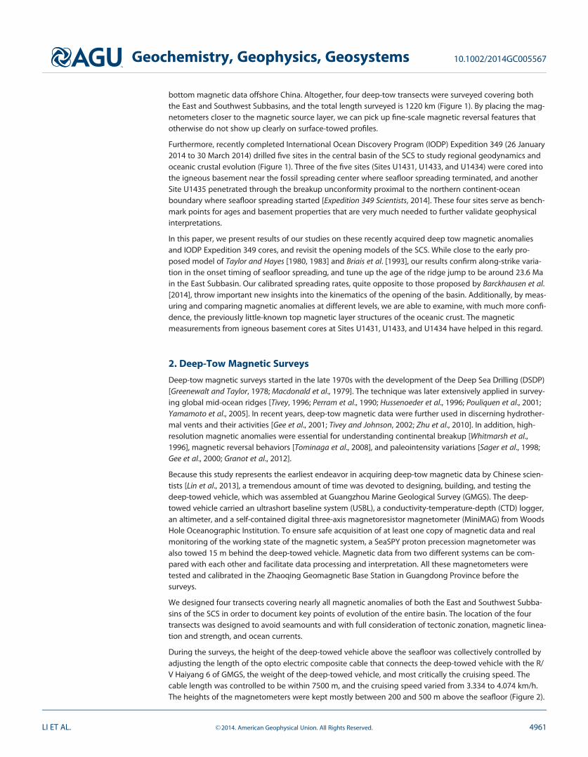
During the surveys, the height of the deep-towed vehicle above the seafloor was collectively controlled byadjusting the length of the opto electric composite cable that connects the deep-towed vehicle with the R/V Haiyang 6 of GMGS, the weight of the deep-towed vehicle, and most critically the cruising speed. Thecable length was controlled to be within 7500 m, and the cruising speed varied from 3.334 to 4.074 km/h.The heights of the magnetometers were kept mostly between 200 and 500 m above the seafloor (Figure 2).



Because of the low cruising speed required, it took R/V Haiyang 6 nearly a month of total work at sea to fin-ish 1220 km of deep tow magnetic survey along four transects: dd12 and de12 acquired in 2012, and dc13and da13 surveyed in 2013 (Figure 1).

Meanwhile, a SeaSPY proton precession magnetic gradiometer was towed �350 m behind the ship torecord magnetic anomalies from the sea surface, which are compared to deep tow magnetic anomalies tobetter calibrate data at different levels. The two magnetometers in the gradiometer were spaced 80 mapart. Although not used and presented in this paper, three-axis shipborne magnetic data were alsoacquired during our surveys by installing fluxgate magnetometers on the mast and GPS antennas.

There are several inland magnetic base stations around the SCS that can provide diurnal corrections to oursurveyed data. We collected their data for data processing. We also deployed a Sentinel seafloor geomag-netic base station in the Zhongsha Islands at a water depth of 2789 m (Figure 1). The station worked wellduring our survey in 2013.

3. Magnetic Data Processing

First, magnetic, navigation, and attitude data are extracted from their respective raw data files and they arethen merged together into one file for each transect. Navigation data are then corrected from the ship posi-tions to the positions of magnetometers based on the recorded lengths of the cables, assuming that thecable runs antiparallel to the heading direction. When the underwater positioning system works well, nonavigation corrections are needed for deep-towed magnetometers.

To remove the theoretical geomagnetic field from the observed data, we apply at 0 m altitude, the softwareGeomag 7.0 and the International Geomagnetic Reference Field (IGRF), which is a spherical harmonic

NE

Sediments

Sediments

U1432

U1435

CO

BC

OB

(a)

dd12

de12

(b)

Figure 2. Estimated basement depths from seismic profiles and towfish depths from deep tow altimeter readings. (a) Transect dd12; (b) Transect de12. COB 5 continent-oceanboundary.



degree 13 model [International Association of Geomagnetism and Aeronomy (IAGA), Working Group V-MOD,2010]. For deep-towed measurements, the software Geomag cannot give geomagnetic intensities for nega-tive altitudes below the sea level, but we find out that the small differences by using geomagnetic intensityat 0 m altitude do not present an issue in magnetic modeling and calibration. For diurnal corrections, werefer data from Zhaoqing and Qiongzhong Geomagnetic Base Stations in Guangdong Province and HainanIsland, respectively (23.093�N, 113.344�E and 19.000�N, 109.800�E), for the year 2012 survey, and for theyear 2013 survey, we use data from Dalat Geomagnetic Observatory in Vietnam (11.945�N, 108.482�E) forsurface-towed data and from the seafloor geomagnetic base station (17.039�N, 115.000�E) for deep-toweddata. We find that diurnal corrections are normally small, mostly within 650.0 nT. These external field cor-rections have longer wavelengths and lower amplitudes than most deep-tow anomalies, and therefore,make little change in the anomaly sequence character [Tominaga et al., 2008].

After all the above corrections, the data are further smoothed with a 100 m wide moving window toremove very short wavelength errors and then resampled to larger sampling intervals. Finally, the magneticanomalies are projected to a common azimuth for each transect. The final processed data are shown in Fig-ures 3–5. Data from both levels are clearly synchronized in their trends. This demonstrates the advantage ofdeep tow magnetic anomalies and also validates the effectiveness of our data acquisition and processingscheme.

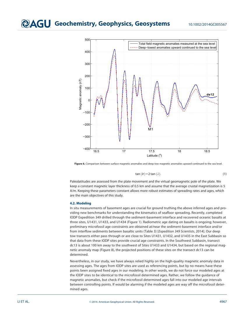
To further see the correlation between surface and deep tow magnetic anomalies, we carry out upwardcontinuation on the deep tow magnetic anomalies from the uneven deep tow level to the sea level usingthe frequency domain chessboard method [Cordell, 1985; Cordell et al., 1993; Phillips, 1997]. The upwardcontinued deep tow magnetic anomalies match remarkably well with the anomalies measured at the sealevel (Figure 6), and can be used to provide a reference in correlating smaller anomalies [Sager et al., 1998;Tominaga et al., 2008].

4. Magnetic Anomaly Modeling and Age Constraints

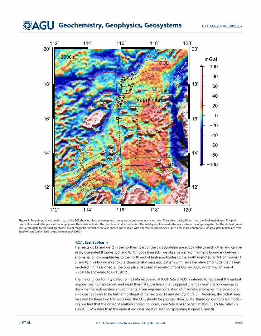
4.1. Model Construction and ParametersBefore constraining SCS crustal ages based on deep tow magnetic anomalies, we need to define thecontinent-ocean boundary (COB) to avoid modeling anomalies that may not be associated with oceaniccrust (Figures 7 and 8). From comprehensive magnetic, gravimetric, and reflection seismic data analyses, Liand Song [2012] found that the COB corresponds roughly with a transitional boundary in free-air gravityanomalies between mostly positive gravity anomalies in the central oceanic basin and grossly negativegravity anomalies in the extended and subsided transitional continental crust (Figure 7). The COB so definedis close to other interpretations [Nguyen et al., 2004; Braitenberg et al., 2006; Franke et al., 2011]. Within thearea confined by the COB, the regional magnetic anomaly map based on the shipborne and airborne mag-netic dataset compiled by Geological Survey of Japan and Coordinating Committee for Costal and OffshoreGeoscience Programs in East and Southeast Asia (CCOP) [Ishihara and Kisimoto, 1996], shows typical alter-nating magnetic reversal patterns (Figure 8).

On or near most segments of our deep-tow magnetic survey lines, we have multichannel reflection seismicprofiles to constrain the depths to the magnetic sources (igneous basement) [Li et al., 2010; Ding et al.,2013]. The thickness of sediments can be estimated from the time-depth curves obtained from sonic log-ging at Site 1148 from ODP Leg 184 [Wang et al., 2000; Li et al., 2008] and at IODP Site U1433 from Expedi-tion 349 [Expedition 349 Scientists, 2014]. Where seismic constraints are not possible, we either use a gradualchange in the basement between two controlling depth points or apply the average basement depthsbased on adjacent data.

To simulate magnetic anomalies, we use the MATLAB based software MODMAG [Mendel et al., 2005], whichis a versatile tool that can accommodate varying spreading rates and asymmetric spreading possibly alter-nating with axial jumps. The computing algorithm of the software is based on Talwani and Heirtzler [1964].

Previous studies suggested that the spreading rates of the SCS are low to intermediate [Taylor and Hayes,1980, 1983; Briais et al., 1993; Song and Li, 2012]. In these scenarios, off-axis intrusions or late-stage lavaflows that move horizontally for a long distance may contaminate preexisting polarity stripes [Tisseau andPatriat, 1981; Mendel et al., 2005]. The deeper part of oceanic crust also cools and becomes magnetized later



than the shallower part [Kidd, 1977]. MODMAG is capable of dealing with these problems by forward model-ing with a fictitious spreading rate that is slower than the real spreading rate, based on the method of Tis-seau and Patriat [1981]. By assigning different contamination coefficients R (0< R <5 1, with 1 for nocontamination), the magnetic source blocks are narrowed corresponding with the fictitious spreading ratebefore modeling, and are put back to their original position after computation [Mendel et al., 2005].

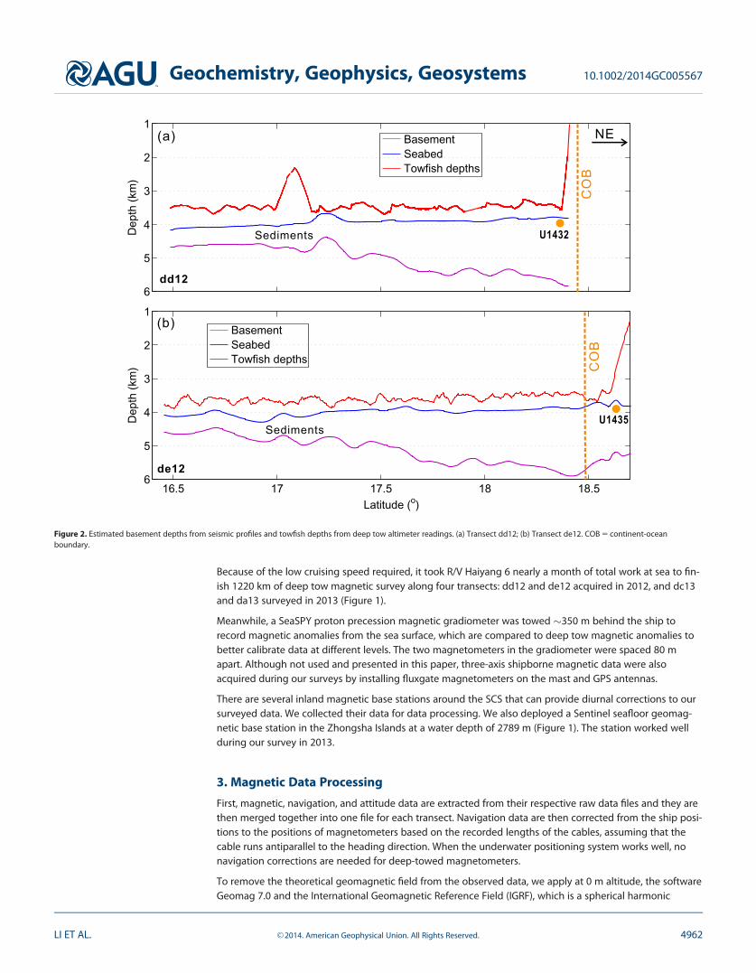
The measurement datum assumed by MODMAG needs to be constant, but our measurements are made onuneven surfaces (Figures 4 and 5). As we show in Figure 6, anomalies of transect de12 upward continued tothe sea level from the uneven deep tow level have an excellent match to anomalies measured at the sealevel, suggesting that unevenness in observation level is not problematic. We can test again on transectde12 how this unevenness affects our observations by upward continuation from the uneven observationsurface to an adjacent level, and we find that the magnetic anomalies after upward continuation to 3.5 kmare very close to the original observation (Figure 3c). This shows that unevenness in our observation does

(b)

M1( )

U1432

U1435

NorthwestSub-basin

East Sub-basin

to -3.5 km

CO

BC

OB

c

de12

dd12

(a)

Figure 3. Comparison between deep tow and surface magnetic anomalies, and correlation between transects dd12 and de12 in the northern part of the SCS. (a) Deep tow magneticanomalies overlaid on a regional magnetic anomaly map based on airborne and shipborne magnetic data; (b) magnetic anomalies of transect dd12; (c) magnetic anomalies of transectde12. COB 5 continent-ocean boundary.



not change the magnetic anomaly patterns and have no effects on data calibration. We therefore opt touse the originally observed instead of leveled anomalies in data calibration.

We adopt the most up-to-date magnetic polarity reversal models from the Geomagnetic Polarity Time Scale2012 (GPTS2012) [Gradstein et al., 2012]. Other information needed for the modeling include ambient mag-netic field components (inclination and declination), spreading direction, azimuth of the profile, depth ofsource layer, and mean latitude and strike of magnetic bodies at the time of ridge formation (Table 2). Theseparameters vary from line to line but can be easily determined from geological and geophysical survey dataand geographical data. The mean ambient magnetic inclinations and declinations are based on the IGRFmodel [International Association of Geomagnetism and Aeronomy (IAGA), Working Group V-MOD, 2010]. Theopening of the SCS is accompanied with southward movement of parts of formed oceanic crust, and it isnecessary to compute the inclination and declination of remanent magnetization vector based on mean lat-itude and strike of magnetic bodies at the time of ridge formation. Assuming a geocentric axial dipole, theremanent inclinations (Ir) are calculated from the mean paleolatitudes (k) based on the following equation[e.g., Mendel et al., 2005]

deep tow (MiniMAG)shipborne

(a)

(b)

( )c

BasementSeabedTowfish depths

N

U1431

U1431

deep tow (SeaSPY)

M2

Spre

adi n

g cen

ter

CO

B

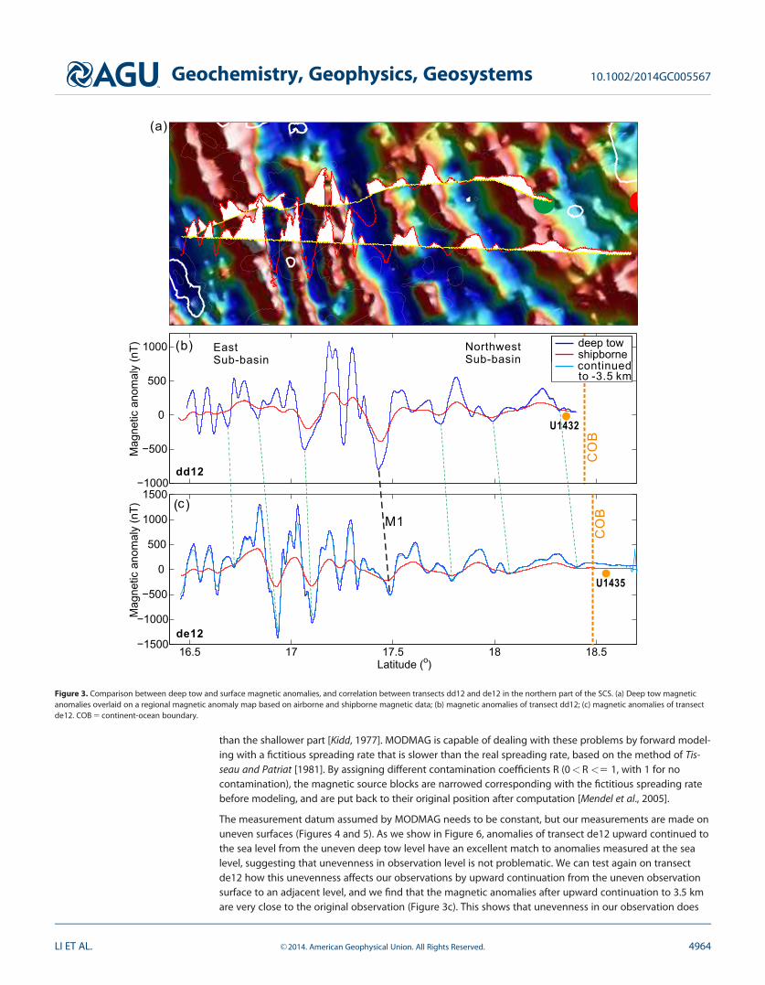
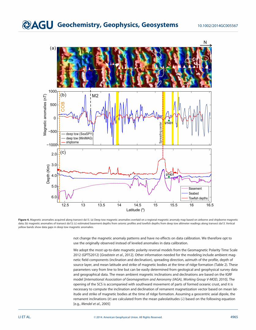
Figure 4. Magnetic anomalies acquired along transect da13. (a) Deep tow magnetic anomalies overlaid on a regional magnetic anomaly map based on airborne and shipborne magneticdata; (b) magnetic anomalies of transect da13; (c) estimated basement depths from seismic profiles and towfish depths from deep tow altimeter readings along transect da13. Verticalyellow bands show data gaps in deep tow magnetic anomalies.



(b)

( )c

(a)

Spre

adin

g cen

ter

NW

BasementSeafloorTowfish depths

shipbornedeep tow (SeaSPY)

CO

B

CO

B

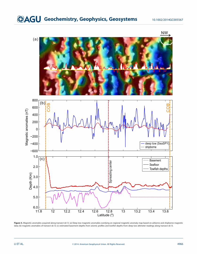
Figure 5. Magnetic anomalies acquired along transect dc13. (a) Deep tow magnetic anomalies overlying on regional magnetic anomaly map based on airborne and shipborne magneticdata; (b) magnetic anomalies of transect dc13; (c) estimated basement depths from seismic profiles and towfish depths from deep tow altimeter readings along transect dc13.



tan Irð Þ52 tan kð Þ: (1)

Paleolatitudes are assessed from the plate movement and the virtual geomagnetic pole of the plate. Wekeep a constant magnetic layer thickness of 0.5 km and assume that the average crustal magnetization is 5A/m. Keeping these parameters constant allows more robust estimates of spreading rates and ages, whichare the main objectives of this study.

4.2. ModelingIn situ measurements of basement ages are crucial for ground truthing the above inferred ages and pro-viding new benchmarks for understanding the kinematics of seafloor spreading. Recently, completedIODP Expedition 349 drilled through the sediment-basement interface and recovered oceanic basalts atthree sites, U1431, U1433, and U1434 (Figure 1). Radiometric age dating on basalts is ongoing; however,preliminary microfossil age constraints are obtained at/near the sediment-basement interface and/orfrom interflow sediments between basaltic units (Table 3) [Expedition 349 Scientists, 2014]. Our deeptow transects either pass through or are close to Sites U1431, U1432, and U1435 in the East Subbasin sothat data from these IODP sites provide crucial age constraints. In the Southwest Subbasin, transectdc13 is about 100 km away to the southwest of Sites U1433 and U1434, but based on the regional mag-netic anomaly map (Figure 8), the projected positions of these sites on the transect dc13 can bedetermined.

Nevertheless, in our study, we have always relied highly on the high-quality magnetic anomaly data inassessing ages. The ages from IODP sites are used as referencing points, but by no means have thesepoints been assigned fixed ages in our modeling. In other words, we do not force our modeled ages atthe IODP sites to be identical to the microfossil determined ages. Rather, we follow the guidance ofmagnetic anomalies, but check if the microfossil determined ages fall into our modeled age intervalsbetween controlling points. If would be alarming if the modeled ages are way off the microfossil deter-mined ages.

M1

de12

Figure 6. Comparison between surface magnetic anomalies and deep tow magnetic anomalies upward continued to the sea level.



4.2.1. East SubbasinTransects dd12 and de12 in the northern part of the East Subbasin are subparallel to each other and can beeasily correlated (Figures 1, 3, and 8). On both transects, we observe a sharp magnetic boundary betweenanomalies of low amplitudes to the north and of high amplitudes to the south (denoted as M1 on Figures 1,3, and 8). This boundary shows a characteristic magnetic pattern with large negative amplitude that is bestmodeled if it is assigned as the boundary between magnetic chrons C8r and C8n, which has an age of�26.0 Ma according to GPTS2012.

The major unconformity dated to �33 Ma recovered at IODP Site U1435 is inferred to represent the earliestregional seafloor spreading and rapid thermal subsidence that triggered changes from shallow marine todeep marine sedimentary environments. From regional correlation of magnetic anomalies, the oldest oce-anic crust appears to be further northeast of transects dd12 and de12 (Figure 8). Therefore, the oldest agesrevealed by these two transects near the COB should be younger than 33 Ma. Based on our forward model-ing, we find that the onset of seafloor spreading locally near Site U1432 began at about 31.5 Ma, which isabout 1.5 Myr later than the earliest regional onset of seafloor spreading (Figures 8 and 9).

COB

M1

M2

da13

dc13

de12dd

12

mGal

Man

ila T

renc

h

?

Fossil ridge

C11r

C10r

C8

C6CrC6Br

C5Cr

C5B

C5En

C6AC6Cr

C8

C9r

C5Cn.1n

C5Cr

C5CrC5Er

C6nC6AAr

C5En

C6n/C6rC6Ar

Figure 7. Free-air gravity anomaly map of the SCS showing deep tow magnetic survey tracks and magnetic anomalies. The yellow dashed lines show the final fossil ridges. The pinkdashed line marks the place of the ridge jump. The arrow indicates the direction of ridge migration. The soild green line marks the place where the ridge migrated to. The dashed greenline is conjugate to the solid green line. Major magnetic anomalies are also shown and marked with anomaly numbers. See Figure 1 for more annotations. Original gravity data are fromSandwell and Smith [2009] and Sandwell et al. [2013].



M1

M2

nT

?

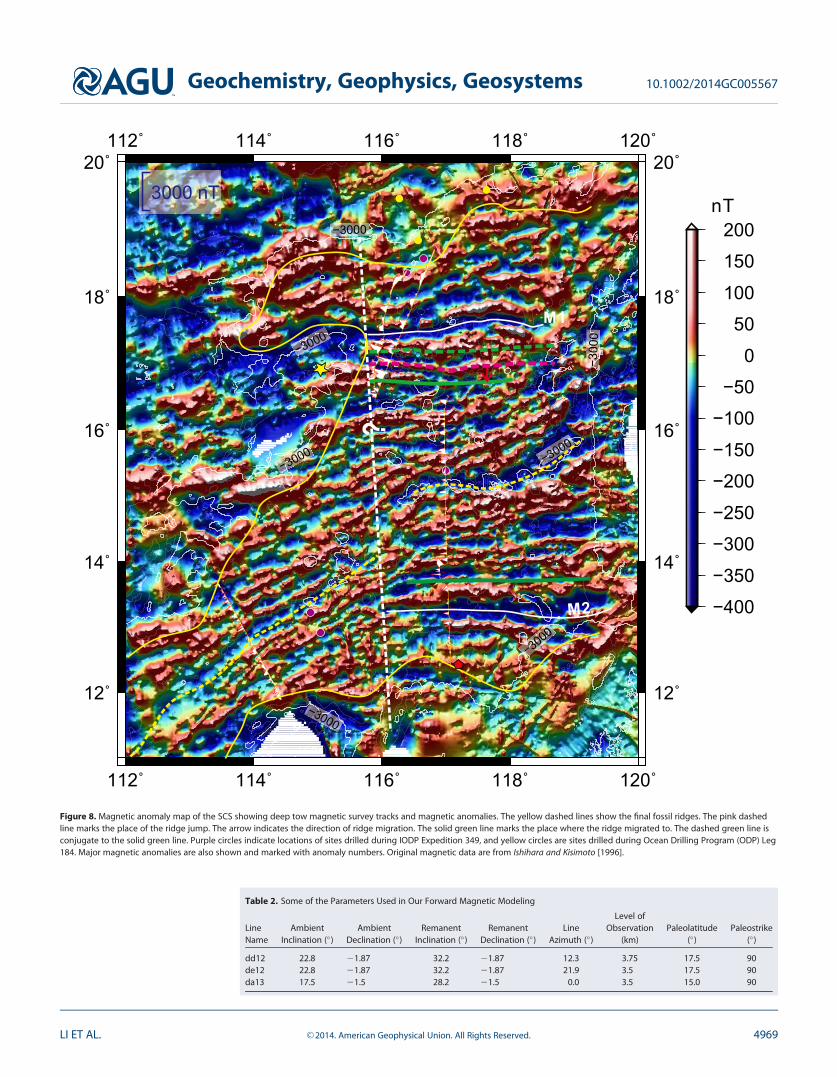
Figure 8. Magnetic anomaly map of the SCS showing deep tow magnetic survey tracks and magnetic anomalies. The yellow dashed lines show the final fossil ridges. The pink dashedline marks the place of the ridge jump. The arrow indicates the direction of ridge migration. The solid green line marks the place where the ridge migrated to. The dashed green line isconjugate to the solid green line. Purple circles indicate locations of sites drilled during IODP Expedition 349, and yellow circles are sites drilled during Ocean Drilling Program (ODP) Leg184. Major magnetic anomalies are also shown and marked with anomaly numbers. Original magnetic data are from Ishihara and Kisimoto [1996].

Table 2. Some of the Parameters Used in Our Forward Magnetic Modeling

LineName

AmbientInclination (�)

AmbientDeclination (�)

RemanentInclination (�)

RemanentDeclination (�)

LineAzimuth (�)

Level ofObservation

(km)Paleolatitude

(�)Paleostrike

(�)

dd12 22.8 21.87 32.2 21.87 12.3 3.75 17.5 90de12 22.8 21.87 32.2 21.87 21.9 3.5 17.5 90da13 17.5 21.5 28.2 21.5 0.0 3.5 15.0 90



Early studies suggested a ridge jump around the anomaly associated with chron C7 [Briais et al., 1993],which could have caused the slightly wider half basin to the north of the fossil axial ridge than to the south.Although this geometrical asymmetry could be explained by asymmetrical spreading rates across the axialridge, by integrated analyses with transect da13 (Figure 10), we now also prefer a ridge jump around 23.6Ma as this arrangement gives the best matches between modeled and observed anomalies (Figures 8–10).The timing of this ridge jump varies slightly from 23.5 to 23.85 Ma based on our modeling of the threetransects in the East Subbasin, and the distance of the jump is about 20 km and also varies slightly fromplace to place.

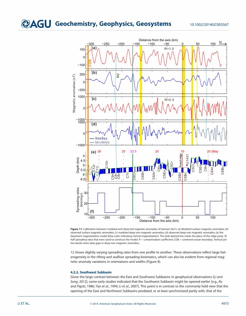
Transect da13 traverses the crust in the central basin that is not covered by transects dd12 and de12. Thisallows modeling of magnetic anomalies over the entire basin without large gaps. During the acquisition ofdata along transect da13, the cable connecting the deep-towed vehicle and the SeaSPY magnetometerdeveloped a leakage problem and had to be fixed several times. This caused narrow data gaps in theSeaSPY data and early pullout of the SeaSPY magnetometer, but both deep-towed MiniMAG and surface-towed magnetometers worked well and recorded excellent data that complement SeaSPY magnetometerreadings (Figure 11).

In a central Pacific study, Barckhausen et al. [2013] compared biostratigraphically determined ages of sedi-ments directly overlying the igneous oceanic crust with confirmed crustal ages based on magnetic anom-aly identifications, and found that consistently the sediment ages are 1–3 Myr younger than themagnetically derived ages. In our case, here at IODP Site U1431, which is about 15 km away from the fos-sil spreading center (Figures 1 and 11), the datable age of sediment above the basement is just about 13Ma. However, radiolarians were found here from interflow sediments between two basaltic units of thebasement, and they were picked from the 63 mm size fraction and examined using scanning electronmicroscope (SEM). The presence of Didymocyrtis prismatica and Calocycletta costata gives an estimatedbiostratigraphy age of �16.7–17.5 Ma (Table 3),which is considered more representative of the age of theunderlying basement [Expedition 349 Scientists, 2014]. The terminal age of the ridge is expected to be a lit-tle younger than this age range. Our modeling suggests that the optimal terminal age in the East Subba-sin is �15.0 Ma (Figure 11).

To the south of the axial ridge, M2 is the sharp magnetic boundary thought to be conjugate to M1. Fromour modeling, we notice that the same boundary between magnetic chrons C8r and C8n creates a posi-tive magnetic anomaly between two large negative anomalies here. This is different from the single largenegative anomaly caused by the same chron boundary to the north of the axial ridge, because of theiropposite relative positions of magnetic chrons C8r and C8n; chron C8n is located to the south of chronC8r north of the fossil ridge, but to the south of the fossil ridge chron C8n is located north of chron C8r(Figures 9–11). With this character, we can easily identity the location of M2, which provides a definitiveage control (Figure 11).

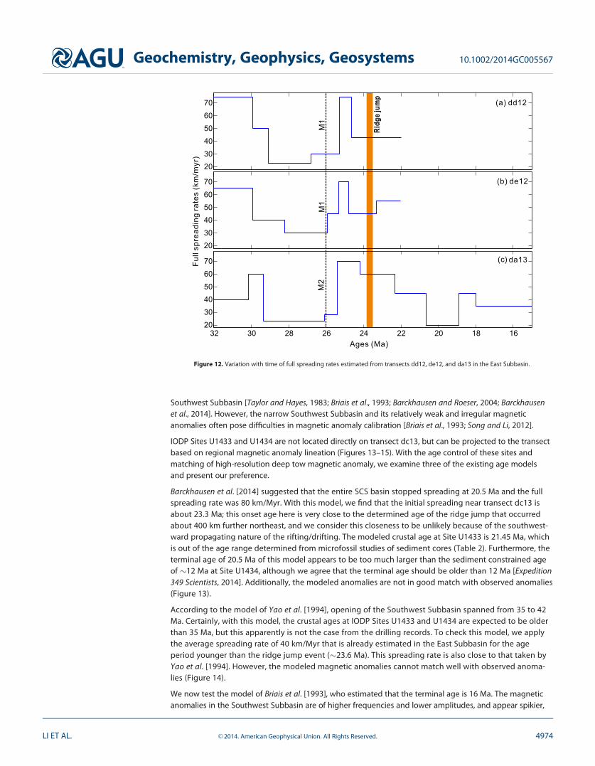
Our modeling results based on the three transects in the East Subbasin indicate that the full spreading ratewas higher at the beginning of seafloor spreading from �32 to �29 Ma (Figure 12). The spreading ratedropped to a low of �25 km/Myr on average from �29 to �26 Ma. Studies in other parts of the oceanicbasin have always indicated abrupt changes in spreading rate [M€uller et al., 2008]. The relatively fast

Table 3. Estimated Ages of Sediment Lying Directly on (Site U1434) or Within Basement (Sites U1431 and U1433), and Estimated Age of Breakup Unconformity at Site U1435, Basedon Biostratigraphy [Expedition 349 Scientists 2014]a

Site Location Biostratigraphic Datums Inferred Age Range For

U1431 15�22.50N, 117�0.00E LO Didymocyrtis prismatica (16.73 Ma) 16.7–17.5 Ma. Frominterflow sediments

Basement�15 km off ridge axis in East Subbasin FO Calocycletta costata (17.59 Ma)

U1433 12�55.10N, 115�02.80E LO Triquetrorhabdulus carinatus (18.28 Ma) 18–21 Ma. From sedimentsattached to basalt

Basement�50 km off ridge axis inSouthwest Subbasin

FO Stichocorys delmontensis (20.6 Ma)

U1434 13�11.50N, 114�55.40E FO Discoaster kugleri (11.9 Ma) 12–18 Ma. From sedimentsoverlying the basement

Basement�15 km off ridge axis inSouthwest Subbasin

U1435 18�33.30N, 116�36.60E LO Coccolithus formosus (32.92 Ma) �33 Ma BreakupunconformityNear continent-ocean boundary LO Clausicoccus distichus acme (33.43 Ma)

aNotes: LO 5 last occurrence; FO 5 first occurrence.



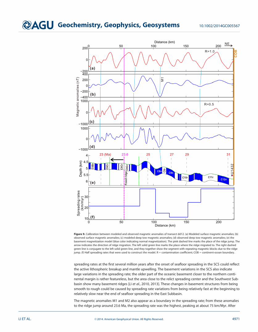
spreading rates at the first several million years after the onset of seafloor spreading in the SCS could reflectthe active lithospheric breakup and mantle upwelling. The basement variations in the SCS also indicatelarge variations in the spreading rate; the older part of the oceanic basement closer to the northern conti-nental margin is rather featureless, but the area close to the relict spreading center and the Southwest Sub-basin show many basement ridges [Li et al., 2010, 2013]. These changes in basement structures from beingsmooth to rough could be caused by spreading rate variations from being relatively fast at the beginning torelatively slow near the end of seafloor spreading in the East Subbasin.

The magnetic anomalies M1 and M2 also appear as a boundary in the spreading rate; from these anomaliesto the ridge jump around 23.6 Ma, the spreading rate was the highest, peaking at about 75 km/Myr. After

M1

(a)

(b)

( )c

(d)

CO

B

NE

R=0.5

R=1.0

U14

32

C8n

C6Cr

C6Cr

C8r

C11rC12nC10r

C9n

C6CrC6

Br

(e) F oss

i l ri d

ge

Spr

eadi

ng r

ates

(km

/myr

)

(f)

Figure 9. Calibration between modeled and observed magnetic anomalies of transect dd12. (a) Modeled surface magnetic anomalies; (b)observed surface magnetic anomalies; (c) modeled deep tow magnetic anomalies; (d) observed deep tow magnetic anomalies; (e) thebasement magnetization model (blue color indicating normal magnetization). The pink dashed line marks the place of the ridge jump. Thearrow indicates the direction of ridge migration. The left solid green line marks the place where the ridge migrated to. The right dashedgreen line is conjugate to the left solid green line, and they together show the segment with repeating magnetic blocks due to the ridgejump. (f) Half spreading rates that were used to construct the model. R 5 contamination coefficient; COB 5 continent-ocean boundary.



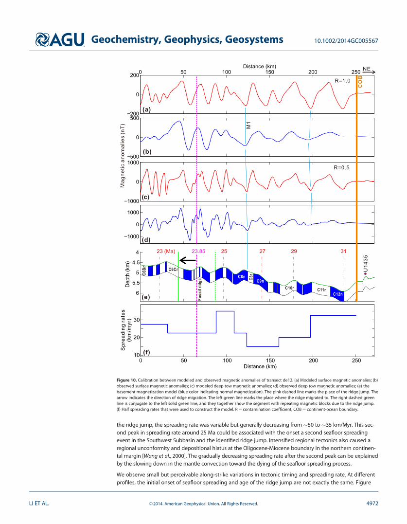
the ridge jump, the spreading rate was variable but generally decreasing from�50 to �35 km/Myr. This sec-ond peak in spreading rate around 25 Ma could be associated with the onset a second seafloor spreadingevent in the Southwest Subbasin and the identified ridge jump. Intensified regional tectonics also caused aregional unconformity and depositional hiatus at the Oligocene-Miocene boundary in the northern continen-tal margin [Wang et al., 2000]. The gradually decreasing spreading rate after the second peak can be explainedby the slowing down in the mantle convection toward the dying of the seafloor spreading process.

We observe small but perceivable along-strike variations in tectonic timing and spreading rate. At differentprofiles, the initial onset of seafloor spreading and age of the ridge jump are not exactly the same. Figure

M1

(b)

(a)

( )c

(d)

(e)

CO

B

NE

U14

35

R=0.5

R=1.0

C12nC11rC10r

C8rC8n

C6Cr

C9n

C6Br

Foss

il r id

ge

(f)Sp r

eadi

ng r

ates

(km

/myr

)

Figure 10. Calibration between modeled and observed magnetic anomalies of transect de12. (a) Modeled surface magnetic anomalies; (b)observed surface magnetic anomalies; (c) modeled deep tow magnetic anomalies; (d) observed deep tow magnetic anomalies; (e) thebasement magnetization model (blue color indicating normal magnetization). The pink dashed line marks the place of the ridge jump. Thearrow indicates the direction of ridge migration. The left green line marks the place where the ridge migrated to. The right dashed greenline is conjugate to the left solid green line, and they together show the segment with repeating magnetic blocks due to the ridge jump.(f) Half spreading rates that were used to construct the model. R 5 contamination coefficient; COB 5 continent-ocean boundary.



12 shows slightly varying spreading rates from one profile to another. These observations reflect large het-erogeneity in the rifting and seafloor spreading kinematics, which can also be evident from regional mag-netic anomaly variations in orientations and widths (Figure 8).

4.2.2. Southwest SubbasinGiven the large contrast between the East and Southwest Subbasins in geophysical observations [Li andSong, 2012], some early studies indicated that the Southwest Subbasin might be opened earlier [e.g., Ruand Pigott, 1986; Yao et al., 1994; Li et al., 2007]. This point is in contrast to the commonly held view that theopening of the East and Northwest Subbasins predated, or at least synchronized partly with, that of the

M2

SeaSpyMiniMAG

Foss

il rid

ge

(b)

(a)

( )c

(d)

(e)

CO

B

N

U14

31

R=0.5

R=1.0

C6B

r

C6A

r

C6n

C5 E

n

C5C

r

C5B

r

C5B

r

C5C

r

C5E

nC6n

C6A

r

C6B

r

C7 r

C6C

r

C8r

C8n

C9n

C10

r

C11

rC

12r

Spr

eadi

ng r

ates

(km

/myr

)

(f)

Figure 11. Calibration between modeled and observed magnetic anomalies of transect da13. (a) Modeled surface magnetic anomalies; (b)observed surface magnetic anomalies; (c) modeled deep tow magnetic anomalies; (d) observed deep tow magnetic anomalies; (e) thebasement magnetization model (blue color indicating normal magnetization). The pink dashed line marks the place of the ridge jump. (f)half spreading rates that were used to construct the model. R 5 contamination coefficient; COB 5 continent-ocean boundary. Vertical yel-low bands show data gaps in deep tow magnetic anomalies.



Southwest Subbasin [Taylor and Hayes, 1983; Briais et al., 1993; Barckhausen and Roeser, 2004; Barckhausenet al., 2014]. However, the narrow Southwest Subbasin and its relatively weak and irregular magneticanomalies often pose difficulties in magnetic anomaly calibration [Briais et al., 1993; Song and Li, 2012].

IODP Sites U1433 and U1434 are not located directly on transect dc13, but can be projected to the transectbased on regional magnetic anomaly lineation (Figures 13–15). With the age control of these sites andmatching of high-resolution deep tow magnetic anomaly, we examine three of the existing age modelsand present our preference.

Barckhausen et al. [2014] suggested that the entire SCS basin stopped spreading at 20.5 Ma and the fullspreading rate was 80 km/Myr. With this model, we find that the initial spreading near transect dc13 isabout 23.3 Ma; this onset age here is very close to the determined age of the ridge jump that occurredabout 400 km further northeast, and we consider this closeness to be unlikely because of the southwest-ward propagating nature of the rifting/drifting. The modeled crustal age at Site U1433 is 21.45 Ma, whichis out of the age range determined from microfossil studies of sediment cores (Table 2). Furthermore, theterminal age of 20.5 Ma of this model appears to be too much larger than the sediment constrained ageof �12 Ma at Site U1434, although we agree that the terminal age should be older than 12 Ma [Expedition349 Scientists, 2014]. Additionally, the modeled anomalies are not in good match with observed anomalies(Figure 13).

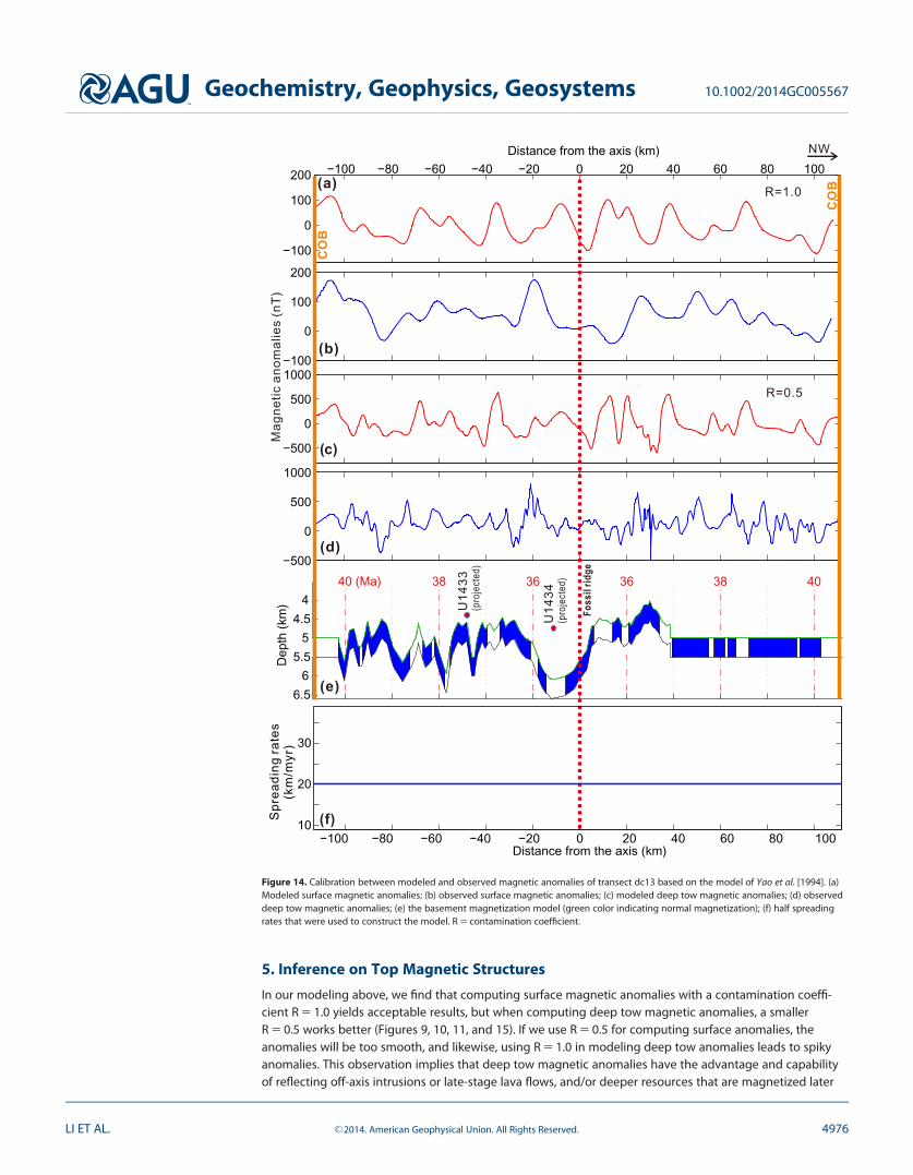
According to the model of Yao et al. [1994], opening of the Southwest Subbasin spanned from 35 to 42Ma. Certainly, with this model, the crustal ages at IODP Sites U1433 and U1434 are expected to be olderthan 35 Ma, but this apparently is not the case from the drilling records. To check this model, we applythe average spreading rate of 40 km/Myr that is already estimated in the East Subbasin for the ageperiod younger than the ridge jump event (�23.6 Ma). This spreading rate is also close to that taken byYao et al. [1994]. However, the modeled magnetic anomalies cannot match well with observed anoma-lies (Figure 14).

We now test the model of Briais et al. [1993], who estimated that the terminal age is 16 Ma. The magneticanomalies in the Southwest Subbasin are of higher frequencies and lower amplitudes, and appear spikier,

Ages (Ma)

Ful

l spr

eadi

ng r

ates

(km

/myr

)

(a) dd12

(b) de12

da13

Ridg

e jum

p

( )c

M1

M1

M2

Figure 12. Variation with time of full spreading rates estimated from transects dd12, de12, and da13 in the East Subbasin.



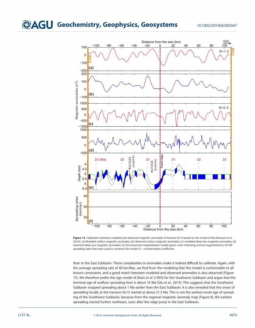
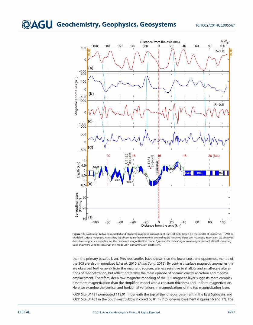
than in the East Subbasin. These complexities in anomalies make it indeed difficult to calibrate. Again, withthe average spreading rate of 40 km/Myr, we find from the modeling that this model is conformable to allknown constraints, and a good match between modeled and observed anomalies is also observed (Figure15). We therefore prefer the age model of Briais et al. [1993] for the Southwest Subbasin and argue that theterminal age of seafloor spreading here is about 16 Ma [Qiu et al., 2014]. This suggests that the SouthwestSubbasin stopped spreading about 1 Ma earlier than the East Subbasin. It is also revealed that the onset ofspreading locally at the transect dc13 started at about 21.5 Ma. This is not the earliest onset age of spread-ing of the Southwest Subbasin, because from the regional magnetic anomaly map (Figure 8), the earliestspreading started further northeast, soon after the ridge jump in the East Subbasin.

(a)

(b)

(d)

(e)

( )c

F oss

il rid

ge

CO

B

CO

B

U1 4

34(p

roje

cted

)

U1 4

33(p

roje

cte d

)

R=0.5

R=1.0

NW

Spr

eadi

ng r

ates

(km

/myr

)

(f)

Figure 13. Calibration between modeled and observed magnetic anomalies of transect dc13 based on the model of Barckhausen et al.[2014]. (a) Modeled surface magnetic anomalies; (b) observed surface magnetic anomalies; (c) modeled deep tow magnetic anomalies; (d)observed deep tow magnetic anomalies; (e) the basement magnetization model (green color indicating normal magnetization); (f) halfspreading rates that were used to construct the model. R 5 contamination coefficient.



5. Inference on Top Magnetic Structures

In our modeling above, we find that computing surface magnetic anomalies with a contamination coeffi-cient R 5 1.0 yields acceptable results, but when computing deep tow magnetic anomalies, a smallerR 5 0.5 works better (Figures 9, 10, 11, and 15). If we use R 5 0.5 for computing surface anomalies, theanomalies will be too smooth, and likewise, using R 5 1.0 in modeling deep tow anomalies leads to spikyanomalies. This observation implies that deep tow magnetic anomalies have the advantage and capabilityof reflecting off-axis intrusions or late-stage lava flows, and/or deeper resources that are magnetized later

NW

CO

B

CO

BR=1.0

R=0.5

Foss

il rid

ge

U14

33(p

roje

cted

)

U14

34(p

roje

cted

)

(e)

(d)

( )c

(b)

(a)

Spr

eadi

ng r

ates

(km

/myr

)

(f)

Figure 14. Calibration between modeled and observed magnetic anomalies of transect dc13 based on the model of Yao et al. [1994]. (a)Modeled surface magnetic anomalies; (b) observed surface magnetic anomalies; (c) modeled deep tow magnetic anomalies; (d) observeddeep tow magnetic anomalies; (e) the basement magnetization model (green color indicating normal magnetization); (f) half spreadingrates that were used to construct the model. R 5 contamination coefficient.



than the primary basaltic layer. Previous studies have shown that the lower crust and uppermost mantle ofthe SCS are also magnetized [Li et al., 2010; Li and Song, 2012]. By contrast, surface magnetic anomalies thatare observed further away from the magnetic sources, are less sensitive to shallow and small-scale altera-tions of magnetization, but reflect preferably the main episode of oceanic crustal accretion and magmaemplacement. Therefore, deep tow magnetic modeling of the SCS magnetic layer suggests more complexbasement magnetization than the simplified model with a constant thickness and uniform magnetization.Here we examine the vertical and horizontal variations in magnetizations of the top magnetization layer.

IODP Site U1431 penetrated 118.01 m beneath the top of the igneous basement in the East Subbasin, andIODP Site U1433 in the Southwest Subbasin cored 60.81 m into igneous basement (Figures 16 and 17). The

(a)

(b)

( )c

(d)

(e)

Fos s

il ri d

ge

CO

B

CO

B

NW

R=0.5

R=1.0

C6ArC6nC5EnC5Cr

C5Dn

C5Cn.1

n

C5Cr

C5EnC6n

C6Ar

Spr

eadi

ng r

ates

(km

/myr

)

(f)

U14

33( p

roj e

cted

)

U14

34(p

r oje

cted

)

Figure 15. Calibration between modeled and observed magnetic anomalies of transect dc13 based on the model of Briais et al. [1993]. (a)Modeled surface magnetic anomalies; (b) observed surface magnetic anomalies; (c) modeled deep tow magnetic anomalies; (d) observeddeep tow magnetic anomalies; (e) the basement magnetization model (green color indicating normal magnetization); (f) half spreadingrates that were used to construct the model. R 5 contamination coefficient.



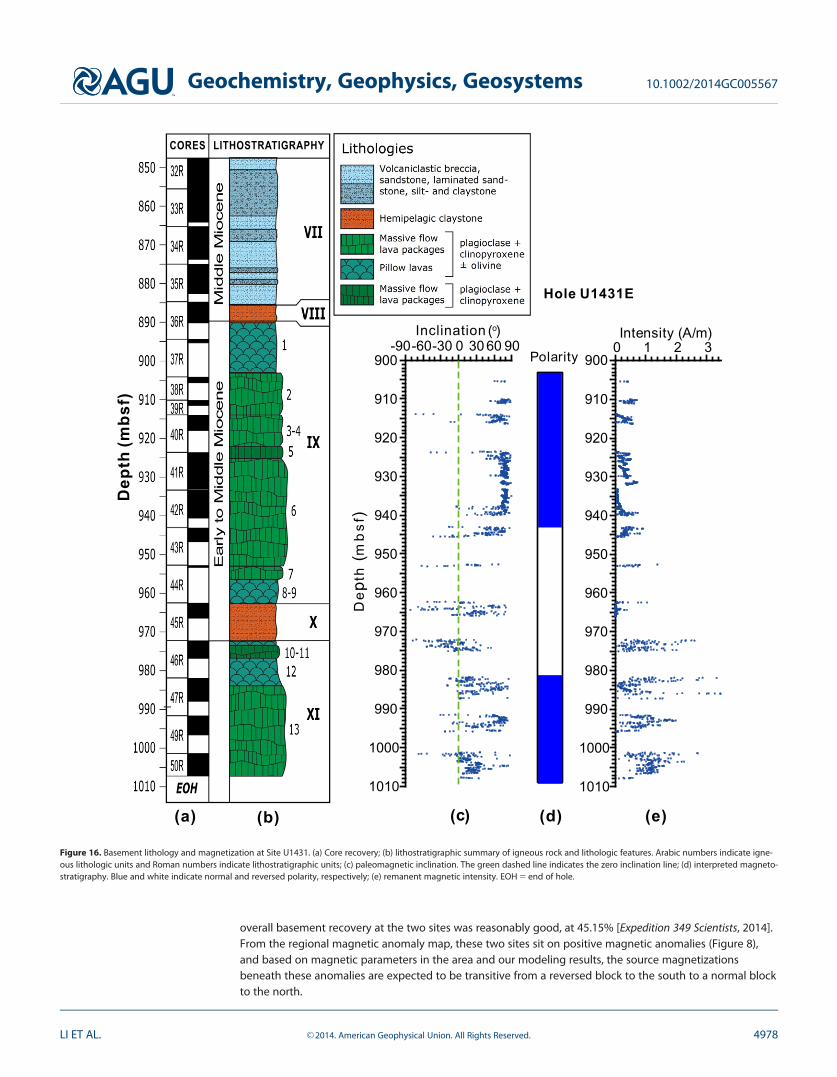
overall basement recovery at the two sites was reasonably good, at 45.15% [Expedition 349 Scientists, 2014].From the regional magnetic anomaly map, these two sites sit on positive magnetic anomalies (Figure 8),and based on magnetic parameters in the area and our modeling results, the source magnetizationsbeneath these anomalies are expected to be transitive from a reversed block to the south to a normal blockto the north.

(a) (b) (d) (e)( )c

Dep

th (m

bsf)

Inclination

Hole U1431E

CORES LITHOSTRATIGRAPHY

Figure 16. Basement lithology and magnetization at Site U1431. (a) Core recovery; (b) lithostratigraphic summary of igneous rock and lithologic features. Arabic numbers indicate igne-ous lithologic units and Roman numbers indicate lithostratigraphic units; (c) paleomagnetic inclination. The green dashed line indicates the zero inclination line; (d) interpreted magneto-stratigraphy. Blue and white indicate normal and reversed polarity, respectively; (e) remanent magnetic intensity. EOH 5 end of hole.



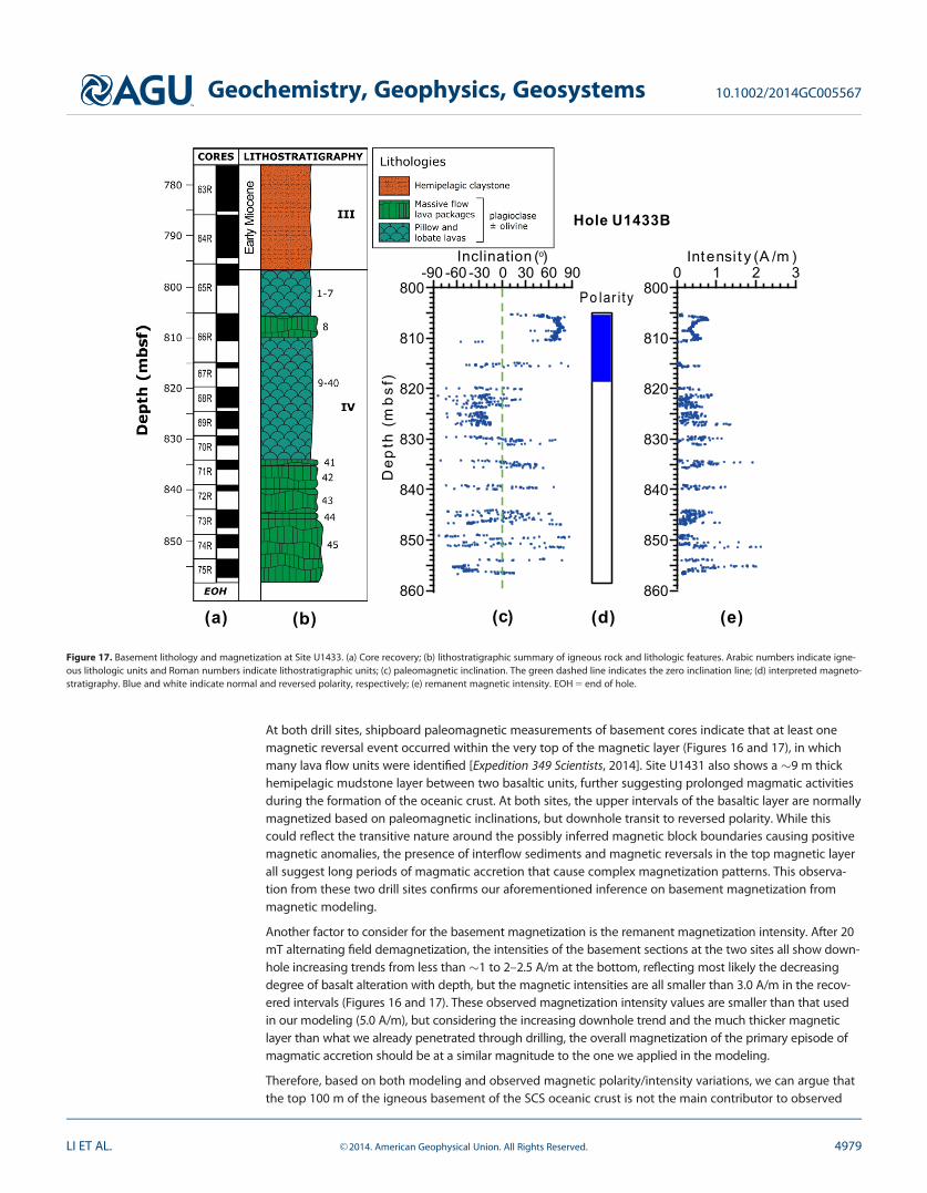
At both drill sites, shipboard paleomagnetic measurements of basement cores indicate that at least onemagnetic reversal event occurred within the very top of the magnetic layer (Figures 16 and 17), in whichmany lava flow units were identified [Expedition 349 Scientists, 2014]. Site U1431 also shows a �9 m thickhemipelagic mudstone layer between two basaltic units, further suggesting prolonged magmatic activitiesduring the formation of the oceanic crust. At both sites, the upper intervals of the basaltic layer are normallymagnetized based on paleomagnetic inclinations, but downhole transit to reversed polarity. While thiscould reflect the transitive nature around the possibly inferred magnetic block boundaries causing positivemagnetic anomalies, the presence of interflow sediments and magnetic reversals in the top magnetic layerall suggest long periods of magmatic accretion that cause complex magnetization patterns. This observa-tion from these two drill sites confirms our aforementioned inference on basement magnetization frommagnetic modeling.

Another factor to consider for the basement magnetization is the remanent magnetization intensity. After 20mT alternating field demagnetization, the intensities of the basement sections at the two sites all show down-hole increasing trends from less than �1 to 2–2.5 A/m at the bottom, reflecting most likely the decreasingdegree of basalt alteration with depth, but the magnetic intensities are all smaller than 3.0 A/m in the recov-ered intervals (Figures 16 and 17). These observed magnetization intensity values are smaller than that usedin our modeling (5.0 A/m), but considering the increasing downhole trend and the much thicker magneticlayer than what we already penetrated through drilling, the overall magnetization of the primary episode ofmagmatic accretion should be at a similar magnitude to the one we applied in the modeling.

Therefore, based on both modeling and observed magnetic polarity/intensity variations, we can argue thatthe top 100 m of the igneous basement of the SCS oceanic crust is not the main contributor to observed

(a) (b) (d) (e)( )c

Inclination

Hole U1433B

Figure 17. Basement lithology and magnetization at Site U1433. (a) Core recovery; (b) lithostratigraphic summary of igneous rock and lithologic features. Arabic numbers indicate igne-ous lithologic units and Roman numbers indicate lithostratigraphic units; (c) paleomagnetic inclination. The green dashed line indicates the zero inclination line; (d) interpreted magneto-stratigraphy. Blue and white indicate normal and reversed polarity, respectively; (e) remanent magnetic intensity. EOH 5 end of hole.



magnetic anomalies that are applicable to age dating. The primary magnetic sources are more deeply bur-ied. This is an important inference on the magnetic structure, and could be applicable to other slow to inter-mediate spreading basins.

Lateral variations in basement magnetization are not directly inverted in this study, but can be easilyassessed from the modeling. We find that, with a constant magnetic intensity of 5.0 A/m, the modeled mag-netic anomalies are mostly matchable to the observed anomalies in their amplitudes. However, to the northof anomaly M1 and to the south of anomaly M2, the modeled anomalies are much higher within the centralbasin, even with the consideration of deepened basement carrying the primary magnetization at theseareas in the modeling, whereas the observed and modeled anomalies in other segments are in similarscales. We attribute this anomaly difference to lower basement magnetizations in the two areas with theoldest crustal ages, which was also indicated previously from 3-D analytical signal analysis [Li et al., 2008].

Parameters accounting for lateral variation in apparent basement magnetization could include basementdepth and composition, alteration of the primary magnetic minerals, long-term changes in the paleomag-netic field intensity, spreading rate and direction, tectonic context, thickness of the magnetic layer, andbasaltic alteration. For profiles de12 and dd12, the amplitude of the magnetic anomalies becomes graduallysmeared from �23 to �31 Ma (Figure 3). However, the modeled magnetic anomalies show rather compara-ble amplitude throughout the profile (Figures 9 and 10). Therefore, the effects of the basement depth onthe magnetic amplitudes can be ruled out since there is not a significant correlation between the amplitudeof the magnetic anomalies and the basement depth.

Channell and Lanci [2014] constructed the Oligocene to Miocene (17.5–26.5 Ma) relative paleomagneticpaleointensity (RPI) for the equatorial Pacific, which exhibits a quasi periodicity of �50 kyr, and typicallyshows high RPI values at �23, 24, and �26 Ma. This pattern seems to be partly consistent with the observeddeep-tow anomalies that also show relatively high amplitudes around these ages (Figures 9 and 10).

Observed magnetic anomalies can reflect changes in the magnetic assemblage in terms of the concentra-tion, domain state, and the degree of low-temperature oxidation. For magnetic particles with grain sizelarger than the superparamagnetic size, the remanence magnetization will be inversely related to grain size[Dunlop and €Ozdemir, 1997; Liu et al., 2012]. Low-temperature oxidation can greatly attenuate the anomalyintensity by the maghemitiztion processes that transform (titano)magnetite to (titano)maghemite [Zhouet al., 2001], and it is reasonable to expect that magnetic particles in older rocks with higher degrees of low-temperature oxidation and alteration have lower magnetic susceptibility [e.g., Wang et al., 2005]. While thiscould explain the low magnetic anomalies in the two areas of the central basin to the north of anomaly M1and to the south of anomaly M2, the sharp boundaries of M1 and M2 seem to be at odds with thissuggestion.

In summary, compositional variations in basement mineralogy and geochemistry appear to be the primaryand most plausible explanation for observed variations in apparent magnetization, whereas spreading ratesand relative paleomagnetic paleointensity could have also contributed to the complexity. From magneticanomalies, it seems that basement rocks are less mafic and lower in magnetic susceptibility in the entirenarrow Southwest Subbasin and in areas adjacent to the continents in the East Subbasin, probably indicat-ing more continental influences on their magma sources [Pautot et al., 1986; Li et al., 2008].

6. Conclusions

Two comprehensive magnetic surveys deploying five sets of different instruments (deep-towed proton pre-cession and three-axis magnetoresistor magnetometers, surface-towed proton precession magnetic gradi-ometer and three-axis fluxgate magnetometer, and seafloor geomagnetic base station) with the newly builtR/V Haiyang 6 acquired 1220 km of deep tow magnetic anomalies for the first time offshore coastal China.These high-resolution and large-amplitude magnetic data along four carefully selected transects, togetherwith discoveries from International Ocean Discovery Program (IODP) Expedition 349 finished in 2014, pro-vide a unique opportunity to reassess current opening models of the SCS.

The earliest opening of the East Subbasin of the SCS started in the northeastern part of the basin around 33Ma based on the age of an unconformity at IODP Site U1435, but the onset of seafloor spreading near IODPSites U1432 and U1435 occurred around 31.5 Ma based on our deep tow magnetic anomaly modeling. This



time difference indicates discontinuous initial spreading along the present-day continent-ocean boundary(COB). The terminal age of seafloor spreading in the East Subbasin is estimated at �15 Ma, and the terminalage is �16 Ma in the Southwest Subbasin.

Modeling results of three deep tow transects support that a ridge jump occurred around 23.6 Ma, thoughvarying slightly in timing from place to place. The distance of this southward jump in spreading center isabout 20 km. It accounts primarily for the asymmetry in basin width across the relict spreading center. Wesuspect that the ridge jump that occurred around 23.6 Ma in the East Subbasin also represents the age ofinitial onset of opening of the Southwest Subbasin. These modeled ages fit well with age constraints basedon microfossils in recovered cores from IODP Expedition 349. Overall, our age model is closer to or moreconsistent with the early models of Taylor and Hayes [1980, 1983] and Briais et al. [1993] than to other pro-posed models.

Our modeling suggests that the full spreading rate in the East Subbasin varies from �20 to �80 km/Myr,putting the SCS into a low to intermediate spreading basin. Spreading started at a relatively high rate andlasted for about 3 Myr, and then dropped to about �25 km/Myr on average from �29 to �26 Ma beforethe occurrence of magnetic anomalies M1 and M2. From M1 and M2 to the ridge jump, the spreading ratemaintained a high rate of about 70 km/Myr, and afterward the spreading rate variably decreased from �50to �35 km/Myr at the end of seafloor spreading. Our calibrated spreading rates are quite opposite to thoseproposed by Barckhausen et al. [2014], who suggested faster spreading rates that even increased after theridge jump to 72 km/Myr in the East Subbasin.

Both deep tow magnetic modeling and measured magnetic polarities from IODP Expedition 349 cores sug-gest late-stage lava flows and/or deeper magnetic sources that were magnetized later in a different polarityfrom that of the primary basaltic layer emplaced during the main phase of crustal accretion. These geologi-cal processes are revealed by measured magnetic anomalies, but more so with deep towed than surface-towed anomalies, implying that deep tow magnetic anomalies are more sensitive to basement complexitiesthan surface anomalies as the deep tow measurements are made closer to the magnetic sources. Weobserve that the primary contributor to apparent magnetization variations is basement mineralogy andgeochemistry, but locally spreading rates and relative paleomagnetic paleointensity may also play second-ary roles.

ReferencesBarckhausen, U., and H. A. Roeser (2004), Seafloor spreading anomalies in the South China Sea revisited, in Continent-Ocean Interactions

Within East Asian Marginal Seas, Geophys. Monogr. Ser., vol. 149, edited by P. Clift et al., pp. 121–125, AGU, Washington, D. C.Barckhausen, U., M. Bagge, and D. S. Wilson (2013), Seafloor spreading anomalies and crustal ages of the Clarion-Clipperton Zone, Mar.

Geophys. Res., 34, 79–88, doi:10.1007/s11001-013-9184-6.Barckhausen, U., M. Engels, D. Franke, S. Ladage, and M. Pubellier (2014), Evolution of the South China Sea: Revised ages for breakup and

seafloor spreading, Mar. Pet. Geol., 599–611, doi:10.1016/j.marpetgeo.2014.02.022.Becker, J. J., et al. (2009), Global bathymetry and elevation data at 30 arc seconds resolution: SRTM30_PLUS, Mar. Geod., 32, 355–371.Braitenberg, C., S. Wienecke, and Y. Wang (2006), Basement structures from satellite-derived gravity field: South China Sea ridge, J. Geo-

phys. Res., 111, B05407, doi:10.1029/2005JB003938.Briais, A., P. Patriat, and P. Tapponnier (1993), Updated interpretation of magnetic anomalies and seafloor spreading stages in the South

China Sea: Implications for the Tertiary tectonics of Southeast Asia, J. Geophys. Res., 98, 6299–6328.Cande, S. V., and D. V. Kent (1995), Revised calibration of the geomagnetic polarity timescale for the late Cretaceous and Cenozoic, J. Geo-

phys. Res., 100, 6093–6095.Channell, J. E. T., and L. Lanci (2014), Oligocene-Miocene relative (geomagnetic) paleointensity correlated from the equatorial Pacific (IODP

Site U1334 and ODP Site 1218) to the South Atlantic (ODP Site 1090), Earth Planet. Sci. Lett., 387, 77–88.Cordell, L. (1985), Techniques, applications, and problems of analytical continuation of New Mexico aeromagnetic data between arbitrary

surfaces of very high relief [abstract], in Proceedings of the International Meeting on Potential Fields in Rugged Topography, Bull. 7, pp.96–99, Inst. of Geophys., Univ. of Lausanne, Lausanne, Switzerland.

Cordell, L., J. D. Phillips, and R. H. Godson (1993), USGS potential-field geophysical software for PC and compatible microcomputers, Lead-ing Edge, 12, 290.

Ding, W., D. Franke, J. Li, and S. Steuer (2013), Seismic stratigraphy and tectonic structure from a composite multi-channel seismic profileacross the entire Dangerous Grounds, South China Sea, Tectonophysics, 582, 162–176.

Dunlop, D. J., and €O. €Ozdemir (1997), Rock Magnetism: Fundamentals and Frontiers, 596 pp., Cambridge Univ. Press, Cambridge, U. K.Expedition 349 Scientists (2014), Opening of the South China Sea and its implications for southeast Asian tectonics, climates, and deep

mantle processes since the late Mesozoic, Int. Ocean Discovery Program Prelim. Rep., 349, 1–109, doi:10.14379/iodp.pr.349.2014.Franke, D., U. Barckhausen, N. Baristeas, M. Engels, S. Ladage, R. Lutz, J. Montano, N. Pellejera, E. G. Ramos, and M. Schnabel (2011), The con-

tinent–ocean transition at the southeastern margin of the South China Sea, Mar. Pet. Geol., 28(6), 1187–1204.Gee, J., S. Webb, J. Ridgway, H. Staudigel, and M. Zumberge (2001), A deep tow magnetic survey of Middle Valley, Juan de Fuca Ridge, Geo-

chem. Geophys. Geosyst., 2(11), 1059, doi:10.1029/2001GC000170.

AcknowledgmentThis paper benefited greatly from thethorough and constructive reviews byRoi Granot and an anonymousreviewer. This research is funded byNational Science Foundation of China(grant 91028007, grant 91428309),Program for New Century ExcellentTalents in University, and ResearchFund for the Doctoral Program ofHigher Education of China (grant20100072110036). This research alsoused samples and/or data provided bythe International Ocean DiscoveryProgram (IODP). We thank the officers,technician, engineers, and crewmembers of R/V Haiyang 6 and D/VJOIDES Resolution for their criticalcontributions. Data mapping issupported by GMT [Wessel and Smith,1995]. Faguang He, Xiaojuan Qu,Shengxuan Liu, Xiuyun Cui, andXiangyu Zhang of GMGS andJiansheng Wu, Jun Chen, XinbingZhang, and Tingting Wang of TongjiUniversity also participated in thedeep tow project. Data related to IODPExpedition 349 will be available fordownloading from the IODP website(www.iodp.org) after the moratoriumperiod, which will end on 30 March2015. Original deep tow magnetic dataused in this study could be availableupon request to the PIs of the deeptow project (C.-F. Li, J. Lin, Z. Sun, andX. Xu), who make the collectivedecision.



http://www.iodp.org

http://dx.doi.org/10.1016/j.marpetgeo.2014.02.022

http://dx.doi.org/10.1029/2005JB003938

http://dx.doi.org/10.14379/iodp.pr.349.2014

http://dx.doi.org/10.1029/2001GC000170

http://www.iodp.org

Gee, J. S., S. C. Cande, J. A. Hildebrand, K. Donnelly, and R. L. Parker (2000), Geomagnetic intensity variations over the past 780 kyr obtainedfrom near-seafloor magnetic anomalies, Nature, 408, 827–832.

Gradstein, F., J. Ogg, and A. Smith (Coords) (2004), A Geologic Time Scale 2004, pp. 1–610, Cambridge Univ. Press, Cambridge, U. K.Gradstein, F. M., J. G. Ogg, M. D. Schmitz, and G. M. Ogg (Coords) (2012), The Geologic Time Scale 2012, 2 volumes plus chart, 1176 pp.,

Elsevier, Boston, Mass.Granot, R., J. Dyment, and Y. Gallet (2012), Geomagnetic field variability during the Cretaceous Normal Superchron, Nat. Geosci., 5, 220–

223.Greenewalt, D., and P. T. Taylor (1978), Near-bottom magnetic measurements between the FAMOUS area and DSDP sites 332 and 333,

Geol. Soc. Am. Bull., 89, 571–576.Hayes, D. E. and S. S. Nissen (2005), The South China Sea margins: Implications for rifting contrasts, Earth Planet. Sci. Lett., 237(3–4),

601–616.Hsu, S.-K., Y. Yeh, W.-B. Doo, and C.-H. Tsai (2004), New bathymetry and magnetic lineations identifications in the northernmost South

China Sea and their tectonic implications, Mar. Geophys. Res., 25(1–2), 29–44.Hussenoeder, S. A., M. A. Tivey, H. Schouten and R. C. Searle (1996), Near-bottom magnetic survey of the Mid-Atlantic Ridge axis, 24–

2440N: Implications for crustal accretion at slow spreading ridges, J. Geophys. Res., 101, 22,051–22,069.International Association of Geomagnetism and Aeronomy (IAGA), Working Group V-MOD (2010), International geomagnetic reference

field: The eleventh generation, Geophys. J. Int., 183, 1216–1230.Ishihara, T., and K. Kisimoto (1996), Magnetic anomaly map of East Asia, scale 1:4.000.000 [CD-ROM], Geol. Surv. of Jpn. and Coord. Comm.

for Costal and Offshore Geosci. Programs in East and Southeast Asia, Tokyo, Japan.Kidd, R. G. W. (1977), The nature and shape of the sources of marine magnetic anomalies, Earth Planet. Sci. Lett., 33(3), 310–320.Li, C.-F., and T. Song (2012), Magnetic recording of the Cenozoic oceanic crustal accretion and evolution of the South China Sea Basin,

Chin. Sci. Bull., 57(24), 3165–3181.Li, C.-F., Z. Zhou, J. Li, H. Hu, and J. Geng (2007), Structures of the northeasternmost South China Sea continental margin and ocean basin:

Geophysical constraints and tectonic implications, Mar. Geophys. Res., 28, 59–79.Li, C.-F., Z. Zhou, J. Li, B. Chen, and J. Geng (2008), Magnetic zoning and seismic structure of the South China Sea ocean basin, Mar. Geo-

phys. Res., 29(4), 223–238.Li, C.-F., et al. (2009), Opening of the South China Sea and its implications for Southeast Asian tectonics since the late Mesozoic-

Introduction to IODP Proposal 735-Full [in Chinese], Adv. Earth Sci., 24(12), 1339–1351.Li, C.-F., X. Shi, Z. Zhou, J. Li, J. Geng, and B. Chen (2010), Depths to the magnetic layer bottom in the South China Sea area and their tec-

tonic implications, Geophys. J. Int., 182(3), 1229–1247.Li, C.-F., J. Lin, and D. K. Kulhanek (2013), South China Sea tectonics: Opening of the South China Sea and its implications for southeast

Asian tectonics, climates, and deep mantle processes since the late Mesozoic, Int. Ocean Discovery Program Sci. Prospectus, 349, 1–111,doi:10.2204/iodp.sp.349.2013.

Li, Q., Z. Jian, and B. Li (2004), Oligocene-Miocene planktonic foraminifer biostratigraphy, Site 1148, northern South China Sea, in Proceed-ings of the Ocean Drilling Program, Scientific Results, vol. 184, edited by W. L. Prell et al., pp. 1–26, Ocean Drill. Program, College Station,Tex.

Lin J., X. Xu, C.-F. Li, Z. Sun, J. Zhu, Z. Zhou, and N. Qiu (2013), First high-resolution near seafloor survey of magnetic anomalies of the SouthChina Sea, Abstract #OS23E-01 presented at AGU Fall Meeting 2013, AGU, San Francisco, Calif.

Liu, Q. S., A. P. Roberts, J. C. Larrasoa~na, S. K. Banerjee, Y. Guyodo, L. Tauxe, and F. Oldfield (2012), Environmental magnetism: Principlesand applications, Rev. Geophys., 50, RG4002, doi:10.1029/2012RG000393.

Macdonald K. C., K. Kastens, F. N. Spiess, and S. P. Miller (1979), Deep tow studies of the Tamayo Transform Fault, Mar. Geophys. Res., 4, 37–70.

McIntosh, K., H. van Avendonk, L. Lavier, W. R. Lester, D. Eakin, F. Wu, C.-S. Liu, and C.-S. Lee (2013), Inversion of a hyper-extended riftedmargin in the southern Central Range of Taiwan, Geology, 41, 871–874.

Mendel, V., M. Munschy, and D. Sauter (2005), MODMAG, a MATLAB program to model marine magnetic anomalies, Comput. Geosci., 31(5),589–597.

M€uller, R. D., M. Sdrolias, C. Gaina, and W. R. Roest (2008), Age, spreading rates, and spreading asymmetry of the world’s ocean crust, Geo-chem. Geophys. Geosyst., 9, Q04006, doi:10.1029/2007GC001743.

Nguyen, N. T., S.-M. Lee, and C. Q. Bui (2004), Satellite gravity anomalies and their correlation with the major tectonic features in the SouthChina Sea, Gondwana Res., 7(2), 407–424.

Pautot, G., C. Rangin, A. Briais, P. Tapponnier, P. Beuzart, G. Lericolais, X. Mathieu, J. Wu, S. Han, H. Li, Y. Lu, and J. Zhao (1986), Spreadingdirection in the central South China Sea, Nature, 321(6066), 150–154.

Perram, L. J., K. C. Macdonald, and S. P. Miller (1990), Deep-tow magnetics near 20 Ma on the East Pacific Rise: A study of short wavelengthanomalies at a very fast spreading center, Mar. Geophys. Res., 12, 235–245.

Phillips, J. D. (1997), Potential-Field Geophysical Software for the PC, version 2.2, open file report, 97–725. U.S. Department of the Interior,U.S. Geol. Surv, Denver, USA. [Available at http://pubs. usgs.gov/of/1997/ofr-97–0725/.]

Pouliquen, G., Y. Gallet, J. Dyment, P. Patriat, and C. Tamura (2001), A geomagnetic record over the last 3.5 million years from deep-towmagnetic anomaly profiles across the Central Indian Ridge, J. Geophys. Res., 6, 10,941–10,960.

Qiu, N., Z. Sun, J. Lin, C.-F. Li, and X. Xu (2014), Geomagnetic polarity reversal model of deeptow magnetic survey in the Southwest Subba-sin of South China Sea ridge, Abstract presented at 2014 AGU Fall Meeting, GP23A-3658, AGU, San Francisco, Calif.

Ru, K., and J. D. Pigott (1986), Episodic rifting and subsidence in the South China Sea, AAPG Bull., 70, 1136–1155.Sager, W. W., C. J. Weiss, M. A. Tivey, and H. P. Johnson (1998), Geomagnetic polarity reversal model of deep-tow profiles from the Pacific

Jurassic Quiet Zone, J. Geophys. Res., 103, 5269–5286.Sandwell, D., E. Garcia, K. Soofi, P. Wessel, M. Chandler, and W. H. F. Smith (2013), Toward 1-mGal accuracy in global marine gravity from

CryoSat-2, Envisat, and Jason-1, Leading Edge, 32(8), 892–899.Sandwell, D. T., and W. H. F. Smith (2009), Global marine gravity from retracked Geosat and ERS-1 altimetry: Ridge segmentation versus

spreading rate, J. Geophys. Res., 114, B01411, doi:10.1029/2008JB006008.Song, T., and C.-F. Li (2012), The opening ages and mode of the South China Sea estimated from high-density magnetic tracks [in Chinese],

Prog. Geophys., 27(4), 1432–1442.Talwani, M., and J. R. Heirtzler (1964), Computation of magnetic anomalies caused by two-dimensional structures of arbitrary shapes, in

Computers in the Mineral Industries, Geol. Sci., vol. 9, pp. 464–479, Stanford Univ. Publ., Calif, USA.



http://dx.doi.org/10.2204/iodp.sp.349.2013

http://dx.doi.org/10.1029/2012RG000393

http://dx.doi.org/10.1029/2007GC001743

http://dx.doi.org/10.1029/2008JB006008

Taylor, B., and D. E. Hayes (1980), The tectonic evolution of the South China Basin, in The Tectonic and Geologic Evolution of Southeast AsianSeas and Islands, Geophys. Monogr. Ser., vol. 23, edited by D. E. Hayes, pp. 89–104, AGU, Washington, D. C.

Taylor, B., and D. E. Hayes (1983), Origin and history of the South China Sea Basin, in The Tectonic and Geologic Evolution of Southeast AsianSeas and Islands (Pt. 2), Geophys. Monogr. Ser., vol. 27, edited by D. E. Hayes, pp. 23–56, AGU, Washington, D. C.

Tisseau, J., and P. Patriat (1981), Identification des anomalies magn�etiques sur les dorsales �a faible taux d’expansion: M�ethode des taux fic-tifs, Earth Planet. Sci. Lett., 52, 381–396.

Tivey, M. A. (1996), Vertical magnetic structure of ocean crust determined from near-bottom magnetic field measurements, J. Geophys.Res., 101, 20,275–20,296.

Tivey, M. A., and H. P. Johnson (2002), Crustal magnetization reveals subsurface structure of Juan de Fuca, Geology, 30(11), 979–982.Tominaga, M., W. W. Sager, M. A. Tivey, and S.-M. Lee (2008), Deep-tow magnetic anomaly study of the Pacific Jurassic Quiet Zone and

implications for the geomagnetic polarity reversal timescale and geomagnetic field behavior, J. Geophys. Res., 113, B07110, doi:10.1029/2007JB005527.

Wang, D., R. Van der Voo, and D. R. Peacor (2005), Low-temperature alteration and magnetic changes of variably altered pillow basalts,Geophys. J. Int., 164(1), 25–35.

Wang, P., et al. (2000), Proceedings of Ocean Drilling Program, Initial Report, vol. 184, Ocean Drill. Program, College Station, Tex.Wessel, P., and W. H. F. Smith (1995), New version of the Generic Mapping Tools (GMT) version 3.0 released, Eos Trans. AGU, 76, 329.Whitmarsh, R. B., P. R. Miles, J.-C. Sibuet, and V. Louvel (1996), Geological and geophysical implications of deep-tow magnetometer obser-

vations near sites 897, 898, 899, 900, and 901 on the west Iberia continental margin, in Proceedings of the Ocean Drilling Program, Scien-tific Results, vol. 149, edited by R. B. Whitmarsh at al., pp. 665–674, Ocean Drill. Program, College Station, Tex.

Yamamoto, M., N. Seama, and N. Isezaki (2005), Geomagnetic paleointensity over 1.2 Ma from deep-tow vector magnetic data across theEast Pacific Rise, Earth Planets Space, 57, 465–470.

Yao, B. (1995), Characteristics and tectonic significance of the Zhongnan-Liyue Fault [in Chinese], Memo. 7, pp. 1–14, Geol. Res. of the SouthChina Sea, Guangzhou, China.

Yao, B., W. Zeng, Y. Chen, X. Zhang, D. E. Hayes, J. Diebold, P. Buhl, and S. Spangler (1994), The Geological Memoir of South China Sea Sur-veyed Jointly by China and USA [in Chinese], pp. 1–204, China Univ. of Geosci. Press, Wuhan, China.

Zhou, W., R. Van der Voo, D. R. Peacor, D. Wand, and Y. Zhang (2001), Low-temperature oxidation in MORB of titanomagnetite to titanoma-ghemite: A gradual process with implications for marine magnetic anomaly amplitudes, J. Geophys. Res., 106, 6409–6421.

Zhu, J., J. Lin, Y. Chen, C. Tao, C. German, D. Yoerger, and M. Tivey (2010), A reduced crustal magnetization zone near the first observedactive hydrothermal vent field on the Southwest Indian Ridge, Geophys. Res. Lett., 37, L18303, doi:10.1029/2010GL043542.



http://dx.doi.org/10.1029/2007JB005527

http://dx.doi.org/10.1029/2007JB005527

http://dx.doi.org/10.1029/2010GL043542

Ages and magnetic structures of the South China Sea constrained by deep tow magnetic surveys and...

Documents

Transcript of Ages and magnetic structures of the South China Sea constrained by deep tow magnetic surveys and...