Part I of James's Account of S. H. Long's Expedition, 1819–1820
Upload
khangminh22Category
view
3download
0
Contents1 Introduction9 Lithostratigraphy
18 Biostratigraphy and paleoenvironment
35 Paleomagnetism38 Geochemistry43 Physical properties55 Stratigraphic correlation and
composite section57 References
KeywordsInternational Ocean Discovery Program, IODP, JOIDES Resolution, Expedition 378, South Pacific Paleogene Climate, Climate and Ocean Change, Site U1553, Campbell Plateau, high-southern latitude, Cenozoic climate history, carbon system dynamics, high CO2 world, Paleocene, Eocene, Oligocene, chronostratigraphy, perturbations, temperature gradients, ocean circulation, intermediate water formation, hydrologic cycling, biological productivity, ice sheet dynamics, plate motion, wind fields
Core descriptions
Supplementary material
References (RIS)
MS 378-102Published 6 February 2022
Funded by NSF OCE1326927
Röhl, U., Thomas, D.J., Childress, L.B., and the Expedition 378 ScientistsProceedings of the International Ocean Discovery Program Volume 378publications.iodp.org
Expedition 378 methods1
U. Röhl, D.J. Thomas, L.B. Childress, E. Anagnostou, B. Ausín, B. Borba Dias, F. Boscolo-Galazzo,S. Brzelinski, A.G. Dunlea, S.C. George, L.L. Haynes, I.L. Hendy, H.L. Jones, S.S. Khanolkar, G.D. Kitch,H. Lee, I. Raffi, A.J. Reis, R.M. Sheward, E. Sibert, E. Tanaka, R. Wilkens, K. Yasukawa, W. Yuan,Q. Zhang, Y. Zhang, A.J. Drury, and C.J. Hollis2
1 Röhl, U., Thomas, D.J., Childress, L.B., Anagnostou, E., Ausín, B., Borba Dias, B., Boscolo-Galazzo, F., Brzelinski, S., Dunlea, A.G., George, S.C., Haynes, L.L., Hendy, I.L., Jones, H.L., Khanolkar, S.S., Kitch, G.D., Lee, H., Raffi, I., Reis, A.J., Sheward, R.M., Sibert, E., Tanaka, E., Wilkens, R., Yasu-kawa, K., Yuan, W., Zhang, Q., Zhang, Y., Drury, A.J., and Hollis, C.J., 2022. Expedition 378 methods. In Röhl, U., Thomas, D.J., Childress, L.B., and the Expedition 378 Scientists, South Pacific Paleogene Climate. Proceedings of the International Ocean Discovery Program, 378: College Sta-tion, TX (International Ocean Discovery Program). https://doi.org/10.14379/iodp.proc.378.102.2022
2 Expedition 378 Scientists’ affiliations.
1. IntroductionThe procedures and tools employed in coring operations and in the various shipboard laboratories of the research vessel (R/V) JOIDES Resolution, including measurements made at the Gulf Coast Repository (GCR) (e.g., X-ray fluorescence [XRF] core scanning) and additional biostratigraphic investigations included in the shipboard data set, are documented here for International Ocean Discovery Program (IODP) Expedition 378. This information applies only to shipboard (and the above mentioned GCR and biostratigraphic) work described in the Expedition reports section of the Expedition 378 Proceedings of the International Ocean Discovery Program volume. Methods for postcruise analyses of Expedition 378 samples and data will be described in separate individual publications. This introductory section of the methods chapter describes procedures and equipment used for drilling, coring, core handling, and sample registration; computation of depth for samples and measurements; and the sequence of shipboard analyses. Subsequent methods sec-tions describe laboratory procedures and instruments in more detail.
Unless otherwise noted, all depths in this volume refer to the meters below seafloor (mbsf ) scale.
1.1. Operations
1.1.1. Site location and holesGPS coordinates from Deep Sea Drilling Project (DSDP) Site 277 were used to position the vessel at Expedition 378 Site U1553. A SyQwest Bathy 2010 CHIRP subbottom profiler was used to mon-itor the seafloor depth on the approach to the site and confirm the depth previously recorded. Once the vessel was positioned at the site, the thrusters were lowered. A positioning beacon was not deployed. Dynamic positioning control of the vessel used navigational input from the GPS weighted by the estimated positional accuracy. The final hole position was the mean position cal-culated from GPS data collected over a significant portion of the time the hole was occupied.
Drill sites are numbered according to the series that began with the first site drilled by the Glomar Challenger in 1968. Starting with Integrated Ocean Drilling Program (ODP) Expedition 301, the prefix “U” designates sites occupied by JOIDES Resolution.
When multiple holes are drilled at a site, hole locations are typically offset from each other by ~20 m. A letter suffix distinguishes each hole drilled at the same site. The first hole drilled is assigned the site number modified by the suffix “A,” the second hole takes the site number and the suffix “B,” and so forth. During Expedition 378, five holes were drilled at Site U1553.
https://doi.org/10.14379/iodp.proc.378.102.2022 publications.iodp.org · 1
U. Röhl et al. · Expedition 378 methods IODP Proceedings Volume 378
https://doi.org/10.14379/iodp.proc.378
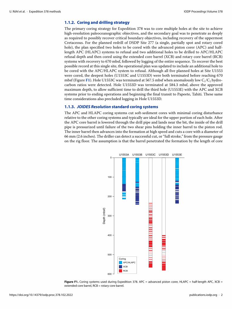
1.1.2. Coring and drilling strategyThe primary coring strategy for Expedition 378 was to core multiple holes at the site to achieve high-resolution paleoceanographic objectives, and the secondary goal was to penetrate as deeply as required to possibly recover critical boundary objectives, including recovery of the uppermost Cretaceous. For the planned redrill of DSDP Site 277 (a single, partially spot and rotary cored hole), the plan specified two holes to be cored with the advanced piston corer (APC) and half-length APC (HLAPC) systems to refusal and two additional holes to be drilled to APC/HLAPC refusal depth and then cored using the extended core barrel (XCB) and rotary core barrel (RCB) systems with recovery to 670 mbsf, followed by logging of the entire sequence. To recover the best possible record at this single site, the operational plan was updated to include an additional hole to be cored with the APC/HLAPC system to refusal. Although all five planned holes at Site U1553 were cored, the deepest holes (U1553C and U1553D) were both terminated before reaching 670 mbsf (Figure F1). Hole U1553C was terminated at 567.5 mbsf when anomalously low C1/C2 hydro-carbon ratios were detected. Hole U1553D was terminated at 584.3 mbsf, above the approved maximum depth, to allow sufficient time to drill the third hole (U1553E) with the APC and XCB systems prior to ending operations and beginning the final transit to Papeete, Tahiti. These same time considerations also precluded logging in Hole U1553D.
1.1.3. JOIDES Resolution standard coring systemsThe APC and HLAPC coring systems cut soft-sediment cores with minimal coring disturbance relative to the other coring systems and typically are ideal for the upper portion of each hole. After the APC core barrel is lowered through the drill pipe and lands near the bit, the inside of the drill pipe is pressurized until failure of the two shear pins holding the inner barrel to the piston rod. The inner barrel then advances into the formation at high speed and cuts a core with a diameter of 66 mm (2.6 inches). The driller can detect a successful cut, or “full stroke,” from the pressure gauge on the rig floor. The assumption is that the barrel penetrated the formation by the length of core
Figure F1. Coring systems used during Expedition 378. APC = advanced piston corer, HLAPC = half-length APC, XCB = extended core barrel, RCB = rotary core barrel.
U1553A U1553B U1553C0
100
500
400
300
200
600
U1553D U1553E
CoringAPC/HLAPC
XCB
RCB
Dep
th (m
bsf)
.102.2022 publications.iodp.org · 2

U. Röhl et al. · Expedition 378 methods IODP Proceedings Volume 378
https://doi.org/10.14379/iodp.proc.378.1
recovered (nominal recovery of ~100%), so the bit is advanced by that length before cutting the next core. The maximum subbottom depth that can be achieved with the APC system (often referred to as “APC refusal”) is limited by the formation stiffness or cohesion and is indicated in two ways: (1) the piston fails to achieve a complete stroke (as determined from the pump pressure reading) because the formation is too hard or (2) excessive force (>100,000 lb; ~267 kN) is required to pull the core barrel out of the formation. Typically, several attempts are made when a full stroke is not achieved. When a full or partial stroke is achieved but excessive force cannot retrieve the barrel, the core barrel is “drilled over,” meaning that after the inner core barrel is successfully shot into the formation, the drill bit is advanced by the length of the APC barrel (~9.6 m).
Nonmagnetic core barrels and the downhole orientation tool (typically deployed except when refusal appears imminent) were employed for Holes U1553A and U1553B. We obtained three for-mation temperature measurements with the advanced piston corer temperature (APCT-3) tool embedded in the APC coring shoe while coring Hole U1553A (Cores 4H, 7H, and 10H). These measurements are applied to calculations of the downhole temperature gradient and heat flow estimates.
The XCB rotary system has a small cutting shoe (bit) that extends below the large rotary APC/XCB bit. The XCB bit is able to cut a semi-indurated core with less torque and fluid circula-tion than the larger main bit, optimizing recovery. The XCB cutting shoe extends ~30.5 cm ahead of the main bit in soft sediment but retracts into the main bit when hard formations are encoun-tered. The resulting cores have a nominal diameter of 5.87 cm (2.312 inches), which is slightly less than the 6.6 cm diameter of APC cores. XCB cores are often broken (torqued) into “biscuits,” which are disc-shaped pieces a few to several centimeters long with remolded sediment (including some drilling slurry) interlayering the discs in a horizontal direction and packing the space between the discs and the core liner in a vertical direction. This type of drilling disturbance may give the impression that the XCB cores have the same thickness (66 mm) as the APC cores. Although both XCB and RCB core recovery (below) generally lead to drilling disturbance in simi-lar sedimentary material, switching from an APC/XCB bottom-hole assembly (BHA) to an RCB BHA requires a pipe trip and adds significant time to the coring operations on site. Thus, we opted to attempt recovery with the XCB coring system as deeply as possible prior to terminating opera-tions in Holes U1553A, U1553B, and U1553E (the three shallow holes).
The RCB system is a conventional rotary coring system suitable for lithified rock material. We opted to use the RCB system exclusively for the two deep holes (U1553C and U1553D) after exploring the efficacy of the XCB coring system in Holes U1553A and U1553B. Increasingly poor recovery with the XCB coring system toward the bottom of Holes U1553A and U1553B precluded deployment for the deeper goals of Holes U1553C and U1553D. Like the XCB system, the RCB system cuts a core with a nominal diameter of 5.87 cm. RCB coring can be done with or without the core liners used routinely with the APC/XCB soft-sediment systems. Coring without liners is sometimes done when core pieces seem to get caught at the edge of the liner, leading to jamming and reduced recovery. During Expedition 378, most RCB cores were drilled with a core liner in place. However, 11 RCB cores were drilled without a liner after recovery became extremely low with a liner in the core barrel.
The BHA is the lowermost part of the drill string. It is typically ~130–170 m long, depending on the coring system used and total drill string length. A typical APC/XCB BHA consists of a drill bit (outside diameter = 117⁄16 inches), a bit sub, a seal bore drill collar, a landing saver sub, a modified top sub, a modified head sub, a nonmagnetic drill collar (for APC/XCB coring), a number of 8¼ inch (~20.32 cm) drill collars, a tapered drill collar, 6 joints (two stands) of 5½ inch (~13.97 cm) drill pipe, and 1 crossover sub. A typical RCB BHA consists of a drill bit, a bit sub, a head sub, an outer core barrel, a top sub, a head sub, 8 joints of 8¼ inch drill collars, a tapered drill collar, 2 stands of standard 5½ inch drill pipe, and a crossover sub to the regular 5 inch drill pipe.
Cored intervals may not be contiguous if separated by intervals that were drilled but not cored. We drilled ahead without coring using a center bit with the RCB system to accelerate penetration because an interval had already been cored in an adjacent hole (234.0 m in Hole U1553C; 399.4 m in Hole U1553D). Holes thus consist of a sequence of cored and drilled intervals, or “advance-
02.2022 publications.iodp.org · 3

U. Röhl et al. · Expedition 378 methods IODP Proceedings Volume 378
https://doi.org/10.14379/iodp.proc.378.
ments.” These advancements are numbered sequentially from the top of the hole downward. Numbers assigned to physical cores correspond to advancements and may not be consecutive.
1.1.4. Drilling disturbanceCores may be significantly disturbed by the drilling process or contain extraneous material as a result of the coring and core handling process. In formations with loose granular layers (sand, ash, foraminifer ooze, chert fragments, shell hash, etc.), drilling circulation may allow granular material from intervals higher in the hole to settle and accumulate in the bottom of the hole. Such material could be sampled by the next core. Therefore, the uppermost 10–50 cm of each core must be assessed for potential “fall-in.”
Common coring-induced deformation includes the concave-downward appearance of originally horizontal bedding. Piston action may result in fluidization (“flow-in”) at the bottom of, or some-times in, APC cores. Retrieval of unconsolidated (APC) cores to the surface typically results to some degree in elastic rebound, and gas that is in solution at depth may become free and drive core segments in the liner apart. When gas content is high, pressure must be relieved for safety reasons before the cores are cut into segments. Holes are drilled into the liner, which forces some sediment and gas out of the liner. As noted above, XCB coring typically results in biscuits mixed with drill-ing slurry. RCB coring typically homogenizes unlithified core material and often fractures lithified core material.
Drilling disturbances are described in Lithostratigraphy in the Site U1553 chapter (Röhl et al., 2022a) and are indicated on graphic core summary reports, also referred to as visual core descrip-tions (VCDs) (see Core descriptions).
1.1.5. Seawater sampling strategySamples for phytoplankton and seawater analysis were collected from international waters during the transit from Site U1553 to Papeete (between 38°37.841′S and 25°36′S) to assess seawater geo-chemistry and the abundance of coccolithophores, foraminifers, and microplastics across a South Pacific Ocean transect. Filtered seawater samples were stored for shore-based geochemical analy-sis and for analysis of shipboard pH, alkalinity, major ions, nutrients, and major elements.
Seawater samples (~20 L) were collected approximately every 12 h at ~0600 and 1830 h (shipboard time) using a plastic bucket with a nylon rope over the side of the ship. The sampling depth approximately represents a mixed upper 10 m of surface water. Latitude and longitude coordinates and the time and date of each collection (in UTC) were recorded. Seawater was stored in a plastic 20 L carboy during filtering. Upon arrival in the laboratory, seawater temperature was measured.
For postcruise coccolithophore assemblage characterization, 1–3 L of seawater was decanted from the 20 L carboy and filtered under gentle pressure through a 47 mm diameter cellulose nitrate filter (0.45 μm pore size). The exact volume of water filtered was recorded to enable species abun-dance per unit seawater to be calculated at a later date. The filtered seawater was then discarded. The filters were dried for 2–4 h at 45°C and stored at room temperature in petri dishes until the end of the expedition. Coccolithophore assemblages will be examined using transmitted light microscopy and scanning electron microscopy (SEM).
For analysis of seawater chemistry, the glass filtration equipment was first rinsed three times with the seawater sample. Then, 1 L of seawater was filtered through a 47 mm, 0.45 μm pore size cellu-lose ester filter. The volume of water filtered was measured using a graduated cylinder and recorded. From this first liter of filtered seawater, samples for shore-based geochemical analysis of δ44Ca, δ17O, iodine speciation, and trace element composition were taken. A split for shipboard analysis of pH and alkalinity as well as ion chromatography measurement of major ions was taken and analyzed (see Geochemistry). For future analysis, samples of minor elements, iodine, and δ44Ca were stored in acid-washed high-density polyethylene bottles.
After sample bottles for geochemistry were filled, another 1 L of water was passed through the first filter. Subsequently, we completed a second filtration of 2 L of water through a new filter. In each case, the volume of water filtered was measured using a graduated cylinder and recorded. The
102.2022 publications.iodp.org · 4

U. Röhl et al. · Expedition 378 methods IODP Proceedings Volume 378
https://doi.org/10.14379/iodp.proc.378.
seawater from both of these steps was discarded. After filtering, filters were removed with twee-zers, placed in petri dishes, and left to dry for ~2–4 h in a low-temperature oven (45°C).
1.2. Core and section handling
1.2.1. Whole-core handlingAll APC, XCB, and RCB cores recovered during Expedition 378 were extracted from the core bar-rel in plastic liners, with the exception of 11 RCB cores from Holes U1553C and U1553D that were collected in split liners on the rig floor. These split liners were carried from the rig floor to the core processing area on the catwalk outside the core laboratory and then closed with the other half of the liner and taped. All cores were then cut into ~1.5 m sections. The exact section length was noted and entered into the database as “created length” using the Sample Master application. This number was used to calculate recovery. Subsequent processing differed for soft-sediment and lith-ified material.
1.2.2. Sediment section handlingHeadspace samples were taken from selected section ends (one per core) using a syringe for imme-diate hydrocarbon analysis as part of the shipboard safety and pollution prevention program. Whole-round samples for interstitial water (IW) analysis were also taken immediately after the core was sectioned. Microbiological sections were taken from the working-half side of the fresh cutting surface (from the top of the adjacent section). Core catcher samples (PALs) were taken for biostratigraphic analysis. When catwalk sampling was complete, liner caps (blue = top, colorless = bottom, and yellow = top of a whole-round sample removed from the section) were glued with acetone onto liner sections and sections were placed in core racks for analysis.
For sediment cores, the curated length was set equal to the created length and was updated very rarely (e.g., in cases of errors or when section length kept expanding by more than ~2 cm). Depths in hole calculations are based on the curated section length (see Depth calculations).
After completion of whole-round section analyses (see Shipboard core analysis), the sections were split lengthwise from bottom to top into working and archive halves. The softer cores were split with a wire, and harder cores were split with a diamond saw. It is important to be aware that older material can be transported upward on the split face of a section during splitting.
1.3. Sample naming
1.3.1. Editorial practiceSample naming in this volume follows standard IODP procedure. A full sample identifier consists of the following information: expedition, site, hole, core number, core type, section number, section half, and offset in centimeters measured from the top of the core section. For example, a sample identification of “378-U1553A-1H-2W, 10–12 cm” represents a sample taken from the interval between 10 and 12 cm below the top of the working half of Section 2 of Core 1 of Hole U1553A during Expedition 378. “H” designates that this core was taken with the full-length APC system, “F” that it was taken with a half-length APC system, “X” that it was taken with an extended core barrel, and “R” that it was rotary drilled.
When working with data downloaded from the Laboratory Information Management System (LIMS) database or physical samples that were labeled on the ship, three additional sample naming concepts may be encountered: text ID, label ID, and printed labels.
1.3.2. Text IDSamples taken on board JOIDES Resolution are uniquely identified for use by software applications using the text ID, which combines two elements:
• Sample type designation (e.g., SHLF for section half) and• A unique sequential number for any sample and sample type added to the sample type code
(e.g., SHLF30495837).
102.2022 publications.iodp.org · 5

U. Röhl et al. · Expedition 378 methods IODP Proceedings Volume 378
https://doi.org/10.14379/iodp.proc.378
The text ID is not particularly helpful to most users but is critical for machine reading and trouble-shooting.
1.3.3. Label IDThe label ID is used throughout the JOIDES Resolution workflows as a convenient, human-readable sample identity. However, a label ID is not necessarily unique. The label ID is made up of two parts: primary sample identifier and sample name.
1.3.3.1. Primary sample identifierThe primary sample identifier is very similar to the editorial sample name described above, with two notable exceptions:
• Section halves always carry the appropriate identifier (378-U1553A-35R-2-A and 378-U1553A-35R-2-W for archive and working half, respectively).
• Sample top and bottom offsets, relative to the parent section, are indicated as “35/37” rather than “35–37 cm.”
Specific rules were set for printing the top offset/bottom offset at the end of the primary sample identifier:
• For samples taken out of the hole, core, or section, top offset/bottom offset is not added to the label ID. This has implications for the common process of taking samples out of the core catcher (CC), which technically is a section (relevant primarily for microbiology and paleontol-ogy samples).
• For samples taken out of the section half, top offset/bottom offset is always added to the label ID. The rule is triggered when an update to the sample name, offset, or length occurs.
• The offsets are always rounded to the nearest centimeter before insertion into the label ID (even though the database stores higher precisions and reports offsets to millimeter precision).
1.3.3.2. Sample nameThe sample name is a free text parameter for subsamples taken from a primary sample or from subsamples thereof. It is always added to the primary sample identifier following a hyphen (-NAME) and populated from one of the following prioritized user entries in the Sample Master application:
1. Entering a sample type (-TYPE) is mandatory (same sample type code used as part of the text ID; see Text ID). By default, -NAME = -TYPE (examples include SHLF, CUBE, CYL, and PWDR).
2. If the user selects a test code (-TEST), it replaces the sample type and -NAME = -TEST. The test code indicates the purpose of taking the sample but does not guarantee that the test was actually completed on the sample (examples include PAL, TSB, ICP, PMAG, and MAD).
3. If the user selects a requester code (-REQ), it replaces -TYPE or -TEST and -NAME = -REQ. The requester code represents the name of the requester of the sample who will conduct post-cruise analysis.
4. If the user types any kind of value (-VALUE) in the -NAME field, perhaps to add critical sample information for postcruise handling, the value replaces -TYPE, -TEST, or -REQ and -NAME = -VALUE (examples include SYL-80deg and DAL-40mT).
In summary, and given the examples above, the same subsample may have the following label IDs based on the priority rule -VALUE > -REQ > -TEST > -TYPE:
• 378-U1553A-35R-2-W 35/37-CYL,• 378-U1553A-35R-2-W 35/37-PMAG,• 378-U1553A-35R-2-W 35/37-DAL, or• 378-U1553A-35R-2-W 35/37-DAL-40mT.
When subsamples are taken out of subsamples, the -NAME of the first subsample becomes part of the parent sample ID, and another -NAME is added to that parent sample label ID:
.102.2022 publications.iodp.org · 6

U. Röhl et al. · Expedition 378 methods IODP Proceedings Volume 378
https://doi.org/10.14379/iodp.proc.37
• Primary_sample_ID-NAME and• Primary_sample_ID-NAME-NAME.
For example, a thin section billet (sample type = TSB) taken from the working half at 40–42 cm offset from the section top might result in a label ID of 378-U1553A-38R-4-W 40/42-TSB. After the thin section was prepared (~48 h later), a subsample of the billet might receive an additional designation of TS05, which would be the fifth thin section made during the expedition. A resulting thin section label ID might therefore be 378-U1553A-38R-4-W 40/42-TSB-TS_5.
1.4. Depth calculationsSample and measurement depth calculations were based on the methods described in IODP Depth Scales Terminology v.2 (https://www.iodp.org/policies-and-guidelines/142-iodp-depth-scales-terminology-april-2011/file) (Table T1). The definition of multiple depth scale types and their distinction in nomenclature should keep the user aware that a nominal depth value at two different depth scale types (and even two different depth scales of the same type) generally does not refer to exactly the same stratigraphic interval in a hole (Figure F2). The SI unit for all depth scales is meter (m).
Depths of cored intervals were measured from the drill floor based on the length of drill pipe deployed beneath the rig floor and are referred to as drilling depth below rig floor (DRF), which is
Table T1. Depth scales used during Expedition 378. mbrf = meters below rig floor, mbsf = meters below seafloor, mcd = meters composite depth. NA = not applicable. CSF-A is only noted if needed to clarify context. Download table in CSV format.
Depth scale type Acronym UnitHistorical reference Figure axis labels Text
Drilling depth below rig floor DRF m mbrf NA NADrilling depth below seafloor DSF m mbsf Depth DSF (m) x m DSFWireline log depth below rig floor WRF m mbrf NA NAWireline log depth below seafloor WSF m mbsf NA NAWireline log speed-corrected depth below seafloor WSSF m mbsf NA NAWireline log matched depth below seafloor WMSF m mbsf Depth WMSF (m) x m WMSFCore depth below seafloor, Method A CSF-A m mbsf Depth CSF-A (m) x m CSF-A/x mbsfCore composite depth below seafloor CCSF m mcd Depth CCSF (m) x m CCSF
Figure F2. Depth scales used during Expedition 378. DRF = drilling depth below rig floor, DSF = drilling depth below sea-floor, CSF-A = core depth below seafloor (Method A), CCSF = core composite depth below seafloor, WRF = wireline log depth below rig floor, WSF = wireline log depth below seafloor, WSSF = wireline log speed-corrected depth below seafloor, WMSF = wireline log matched depth below seafloor.
Rig floor
Sea level
Seafloor
Stratigraphictarget
Water depth (m)
Depth (m)
Seafloor depth(multiple methods)
Tool-specific depth scale types
Seafloorreferenced
WSSF
Laboratoryprocessing-baseddepth scale types
Rig floorreferenced
DRF DSF
WRF WSF WMSF
CSF-A CCSFDrilling depth
Wireline log depth
8.102.2022 publications.iodp.org · 7

U. Röhl et al. · Expedition 378 methods IODP Proceedings Volume 378
https://doi.org/10.14379/iodp.proc.378
traditionally referred to with custom units of meters below rig floor (mbrf ). The depth of each cored interval, measured on the DRF scale, can be referenced to the seafloor by subtracting the seafloor depth measurement (in DRF) from the cored interval (in DRF). This seafloor-referenced depth of the cored interval is referred to as the drilling depth below seafloor (DSF), with a tradi-tionally used custom unit designation of mbsf. In the case of APC coring, the seafloor depth was the length of pipe deployed minus the length of the mudline core recovered. In the case of RCB coring, the seafloor depth was adopted from a previous hole drilled at the site or by tagging the seafloor.
Depths of samples and measurements in each core were computed based on a set of rules that result in a depth scale type referred to as core depth below seafloor, Method A (CSF-A). The two fundamental rules are that (1) the top depth of a recovered core corresponds to the top depth of its cored interval (top DSF = top CSF-A) regardless of the type of material recovered or drilling dis-turbance observed and (2) the recovered material is a contiguous stratigraphic representation even when core segments are separated by voids when recovered, when the core is shorter than the cored interval, or when it is unknown how much material is missing between core pieces. When voids were present in the core on the catwalk, they were closed by pushing core segments together whenever possible. The length of missing core should be considered a depth uncertainty when analyzing data associated with core material.
When core sections were given their curated lengths, they were also given a top and a bottom depth based on the core top depth and the section length. Depths of samples and measurements on the CSF-A scale were calculated by adding the offset of the sample (or measurement from the top of its section) to the top depth of the section.
Per IODP policy established after the introduction of the IODP Depth Scales Terminology v.2, sample and measurement depths on the CSF-A depth scale type are commonly referred to with the custom unit mbsf, just like depths on the DSF scale type. The reader should be aware, however, that the use of mbsf for different depth scales can cause confusion in specific cases because differ-ent “mbsf depths” may be assigned to the same stratigraphic interval. A core composite depth below seafloor (CCSF-A) scale can be constructed to mitigate inadequacies of the CSF-A scale for scientific analysis and data presentation. The most common application is the construction of a CCSF-A scale from multiple holes drilled at a site using depth shifting of correlative features across holes. This method not only eliminates the CSF-A core overlap problem but also allows splicing of core intervals such that gaps in core recovery, which are inevitable in coring a single hole, are essentially eliminated and a continuous stratigraphic representation is established. This depth scale was used at Site U1553 (see Stratigraphic correlation and composite section).
A CCSF-A scale and stratigraphic splice are accomplished by downloading correlation data from the expedition (LIMS) database using the Correlation Downloader application, correlating strati-graphic features across holes using Correlator or any other application and depth-shifting cores to create an “affine table” with an offset for each core relative to the CSF-A scale and a “splice interval table” that defines which core intervals from the participating holes make up the stratigraphic splice. Affine and splice interval tables were uploaded to the LIMS database, where internal com-putations created a CCSF depth scale. The CCSF depth can then be added to all subsequent data downloads from the LIMS database, and data can be downloaded for a splice.
1.5. Shipboard core analysisWhole-round core sections were immediately run through the Whole-Round Multisensor Logger (WRMSL), which measures P-wave velocity, density, and magnetic susceptibility (MS), and the Natural Gamma Radiation Logger (NGRL). For some holes, whole-round core sections were scanned on the X-Ray Multisensor Logger (XMSL) while the cores thermally equilibrated. After the cores thermally equilibrated for at least 4 h, thermal conductivity measurements were also taken before the cores were split lengthwise into working and archive halves. The working half of each core was sampled for shipboard analysis, routinely for paleomagnetism and physical proper-ties and more irregularly for geochemistry and biostratigraphy. The archive half of each core was scanned on the Section Half Imaging Logger (SHIL). Archive halves were also measured for color
.102.2022 publications.iodp.org · 8
U. Röhl et al. · Expedition 378 methods IODP Proceedings Volume 378
https://doi.org/10.14379/iodp.proc.378.
reflectance and MS on the Section Half Multisensor Logger (SHMSL). Archive halves were described macroscopically and microscopically in smear slides. Finally, archive halves were run through the cryogenic magnetometer. Both halves of the core were then put into labeled plastic tubes that were sealed and transferred to cold storage space aboard the ship.
A total of 1962 samples were taken for shipboard analysis. At the end of Expedition 378, all core sections and thin sections were shipped to the GCR in preparation for XRF core scanning to pre-pare a spliced composition section, followed by a shore-based sampling party. The sections and samples will be permanently stored in the GCR.
2. LithostratigraphyThe lithology of sediment recovered during Expedition 378 was primarily determined using observations based on visual (macroscopic) core description, smear slides, and thin sections. Digital core imaging, color reflectance spectrophotometry, MS analysis, and in some cases X-ray diffraction (XRD), XRF, SEM, and carbonate content measurements (see Geochemistry) provided complementary descriptive information. The methods employed during this expedition were sim-ilar to those used during Integrated Ocean Drilling Program Expedition 346 (Tada et al., 2015) and IODP Expedition 379 (Gohl et al., 2021). We used the DESClogik application (version 16.2.0.0) to record and upload visual descriptive data into the LIMS database (see the DESClogik user guide at http://iodp.tamu.edu/labs/index.html; select User guides and laboratory manuals (Confluence) and then select Core Description). Spreadsheet templates were set up in DESClogik and custom-ized for Expedition 378 before the first core on deck. The templates were used to record VCDs as well as microscopic data from smear slides and thin sections, which were also used to quantify the texture and relative abundance of biogenic and nonbiogenic components. The locations of all smear slide and thin section samples taken from each core were recorded in the Sample Master application.
The standard method of splitting cores into working and archive halves (using either a piano wire or a saw) can affect the appearance of the split core surface and obscure fine details of lithology and sedimentary structure. Prior to visual description and imaging of sediments, the archive halves of soft-sediment cores were gently scraped across, rather than along, the core section using a stainless steel or glass scraper to prepare the surface for unobscured sedimentologic examination and description, digital imaging, point MS (MSP), and color measurements. Scraping parallel to bedding with a freshly cleaned tool prevented cross-stratigraphic contamination. Cleaned archive halves were imaged as soon as possible after splitting using the SHIL. Thereafter, archive halves were visually described and analyzed using the SHMSL.
2.1. Visual core descriptionsVCDs of the archive halves of the split cores provide a visual overview of the descriptive litho-stratigraphic, biostratigraphic, and physical properties data obtained during shipboard analyses (Figure F3). All associated data are uploaded to the LIMS database.
Site, hole, and core depth below seafloor, calculated using Method A (CSF-A), are shown at the top of each VCD. Core depths are reported in mbsf, and the depth of core sections is indicated along the left margin. Physical core descriptions correspond to entries in DESClogik, including bioturbation intensity, macrofossils, sedimentary structures, diagenetic constituents, and drilling disturbance. Symbols used in the VCDs are shown in Figure F4. Additionally, sedimentary VCDs display bulk density, MS, natural gamma radiation (NGR), color reflectance, and the locations of samples taken for shipboard measurements. VCDs for Holes U1553C and U1553D also show visual grain size classifications. The written description for each core contains a succinct overview of major and minor lithologies, the Munsell colors, and notable features such as sedimentary structures and major disturbances resulting from the coring process.
2.1.1. Section summaryA brief overview of major and minor lithologies present in this section, along with notable features (e.g., sedimentary structures), is presented in the section summary text field at the top of the VCD.
102.2022 publications.iodp.org · 9

U. Röhl et al. · Expedition 378 methods IODP Proceedings Volume 378
The summary includes sediment color determined qualitatively using Munsell soil color charts.Because sediment color may evolve during drying and subsequent oxidation, color was describedshortly after the cores were split and imaged. However, cores from deeper than Cores 378-U1553C-35R and 378-U1553D-10R only revealed distinct lithologic color changes and detailedsedimentary features after many hours of drying (see Lithostratigraphy in the Site U1553 chapter[Röhl et al., 2022a]). Accordingly, sediment color was obtained only after the archive-half surfaceshad fully dried. For these cores, the section-half images and red-green-blue (RGB) color data thatwere obtained both initially (commented as “regular” in LIMS) and after the surface was fully dry(commented as “dried” in LIMS) are accessible through the LIMS database.
2.1.2. Section-half imageAfter the water used during cutting had dried, the flat faces of the archive halves were scannedwith the SHIL as soon as possible after splitting (and scraping, if necessary) to minimize colorchanges caused by sediment oxidation and/or drying. Exceptions are the cores from deeper thanCores 378-U1553C-35R and 378-U1553D-10R, which revealed previously unobservable sedimen-tary features and structures upon drying (see above). The SHIL uses three pairs of advanced illu-mination high-current-focused LED line lights to illuminate large cracks and blocks in the coresurface. Each LED pair has a color temperature of 6,500 K and emits 90,000 lx at 3 inches. A line-
Figure F3. Example visual core description summarizing data from core imaging, macroscopic and microscopic description, and physical property measurements,Expedition 378. GRA = gamma ray attenuation, cps = counts per second.
zRP8
-9AE
2N
P10
- CN
E2
NANNO
SED
NANNO
SED
NANNO
SED
SED
PALFORAM
RADSNANNO
Early
Eoc
ene
IV
1
2
3
4
5
6
CC
0
100
200
300
400
500
600
700
800
436
435
434
433
432
431
430
429
Naturalgammaradiation
(cps)403020100
Magneticsusceptibility
(IU)9630-3
1050-5
100-10
Reflectancea* b*GRA
bulk density(g/cm3)
2.21.81.4
Dis
turb
ance
inte
nsity
Dis
turb
ance
type
Rad
iola
rian
zone
Plan
ktic
fora
m z
one
Nan
nofo
ssil
zone
Bioturbationintensity
543210
Dia
gene
tic c
onst
ituen
tLi
thol
ogic
acc
esso
ries
Sedi
men
tary
stru
ctur
es
Grain size
7654321
Finer Coarser
Graphiclithology
CoreimageSh
ipbo
ard
sam
ples
Age
Lith
olog
ic u
nit
Sect
ion
Cor
e le
ngth
(cm
)
Dep
th C
SF-A
(m)
Core U1553D-5R is composed of nannofossil chalk, clayey nannofossil chalk, and limestone. The transition to limestone occurs in Section 4, where the sedimentsbecome too hard to use a toothpick for smear slide sampling. The sediments alternate between diffuse greenish-gray sections (10GY 7/1-8/1, 5G 8/1, and 5GY 7/1-8/1)and whiter ones (N 8; on the order of 0.5-1 m of sediment.). The contacts between these layers are bioturbated, with obvious white burrows in green matrix and viceversa. Trace fossils of Teichichnus are observed in Section 2. Very small specks of pyrite are visible, with some larger sections associated with burrow structures.Quartz, feldspar, mica, glauconite, micrite, fish remains, and organic matter were observed in smear slides. There is a chert layer with chalk inclusions in Section 2, andthere are slickensides structures visible in a fracture at the top of Section 4.
Hole 378-U1553D Core 5R, Interval 428.5-436.92 m (CSF-A)
https://doi.org/10.14379/iodp.proc.378.102.2022 publications.iodp.org · 10

U. Röhl et al. · Expedition 378 methods IODP Proceedings Volume 378
scan camera imaged 10 lines per millimeter to create a high-resolution TIFF file. The cameraheight was adjusted so that each pixel imaged a 0.1 mm2 section of the core. However, actual corewidth per pixel varied because of differences in section-half surface height. High- and low-resolu-tion JPEG files were subsequently created from the high-resolution TIFF file. All image filesinclude a gray scale and ruler. Section-half depths were recorded so that these images could beused for core description and analysis.
Figure F4. Symbols used for visual core descriptions, Expedition 378.
Principal lithology
Foraminiferal ooze
Nannofossil ooze
Nannofossil chalk
Calcareous ooze
Calcareous chalk
Indurated sediment
Sand
Chert
Flint
Jasper
Limestone
Mudstone
Sandstone
Packstone
Wackestone
Dolomite
Principal lithology prefix
Foraminifer-rich
Nannofossil-rich
Sandy
Volcanic ash-rich
Carbonate-rich
Dolomitic
Calcareous
Clayey
Principal lithology suffix
with foraminifers
with biosilica
with volcanic ash and foraminifers
with nannofossils
with nannofossils and foraminifers
with quartz
with clay
with sand
Sedimentary structures
Patch or bleb
Lens or pod
Color banding
Parallel lamination
Parallel stratification
Horizontal stratification
Very thin bed
Thin bed
Thin lamination
Medium lamination
Thick lamination
Massive
Layering
Tilted bedding
Normal grading
Grain composition layering
Grain packing layering
Uniform
Lamination
Planar lamination
Irregular bedding
Wavy ripple
Drilling disturbance type
Fall-in
Flow-in
Crack
Fractured
Brecciated
Soupy
Biscuit
Suck in
Bowed
Up-arching
Washed
Drilling disturbance intensity
Slight
Moderate
High
Severe
Diagenetic constituent
Nodule
Concretion
Cement
Mineral
Vein fill
Lithologic accessories
Mineral
Glauconite
Pyrite
Chert
Chlorite
Volcaniclastic
Secondary minerals
Alteration mineral
Diagenetic composition
Pyrite
Carbonate
Alteration mineral
Clay
Calcite
Glauconite
Geothite
Zeolite
Bioturbation intensity rank
No bioturbation was detected
Very slight bioturbation (<5%–10%)
Slight bioturbation (10%–30%)
Moderate bioturbation (30%–60%)
0
3
2
1
Shipboard samples
Carbonate
Foraminifer
Headspace gas
Interstitial water
Moisture and density
Nannofossil
Paleomagnetism
Radiolarian
Paleontology
Rhizon
Sedimentary smear slide
Thin section
X-ray diffraction
Thin section billet
Grain size rank
Clay <3.9 µm/Silt 3.9–63 µm
Very fine sand 63–125 µm
Fine sand 125–250 µm
Medium sand 250–500 µm
1
4
3
2
Coarse sand 0.5–1 mm5
Heavy bioturbation (60%–90%)4
Extensive bioturbation (>90%)5
Very coarse sand 1–2 mm6
Granule 2–4 mm/Pebble 4–64 mm/Cobble 64–256 mm
7
Calcite
https://doi.org/10.14379/iodp.proc.378.102.2022 publications.iodp.org · 11

U. Röhl et al. · Expedition 378 methods IODP Proceedings Volume 378
https://doi.org/10.14379/iodp.proc.378
2.1.3. Graphic lithologyLithologies of the core intervals recovered are represented on the VCDs by graphic patterns in the Graphic lithology column (Figure F4) to scale for all beds that are at least 2 cm thick. Modifiers of primary lithologies are shown in narrow columns to the left (major = prefix) and right (minor = suffix) using the same lithology patterns. Lithologic abundances are recorded in DESClogik and are rounded to the nearest 5%. In the interest of VCD readability, secondary lithologies are not shown, but they are accessible using the LIMS database. Relative abundances of lithologies reported in this way are useful for general characterization of the sediment but do not constitute precise quantitative observations.
2.1.4. Sedimentary structuresThe locations and types of stratification and sedimentary structures visible on the prepared sur-faces of the split cores are shown in the Sedimentary structures column of the VCD sheet. Symbols in this column indicate the locations and scales of interstratification as well as the locations of individual bedding features and any other sedimentary features such as stratification, lamination, and color banding (Figure F4). Relative abundance of commonly observed green millimeter- to centimeter-scale layers was also regularly noted in the Minor lithology description in DESClogik (see Principal names and modifiers). For Expedition 378, the following terminology (based on Stow, 2005) was used to describe the scale of stratification:
• Thin lamination = <0.3 cm thick.• Medium lamination = 0.3–0.6 cm thick.• Thick lamination = 0.6–1 cm thick.• Very thin bed = 1–3 cm thick.• Thin bed = 3–10 cm thick.• Medium bed = 10–30 cm thick.• Thick bed = 30–100 cm thick.• Very thick bed = >100 cm thick.
Descriptive terms for bed boundaries, such as sharp, erosive, gradual, undulating/wavy, and bio-turbated, are noted in DESClogik.
2.1.5. Lithologic accessoriesLithologic, diagenetic, and paleontologic accessories such as nodules, sulfides, and shells are indi-cated on the VCDs. The symbols used to designate these features are shown in Figure F4.
Features interpreted to be diagenetic, including minerals, nodules, concretions, halos, and layer-ing, were noted in DESClogik.
2.1.6. Bioturbation intensitySix levels of bioturbation are recognized using a scheme similar to that of Droser and Bottjer (1986). These levels are illustrated with a numeric scale in the Bioturbation intensity column on the VCDs. Any identifiable trace fossils (ichnofossils) are identified in the bioturbation comments or the general interval comment in the core description.
• 0 = no bioturbation was detected, or level could not be determined.• 1 = very slight bioturbation (<5%–10%).• 2 = slight bioturbation (10%–30%).• 3 = moderate bioturbation (30%–60%).• 4 = heavy bioturbation (60%–90%).• 5 = extensive bioturbation (>90%).
2.1.7. Sediment disturbanceDrilling-related sediment disturbance is recorded in the Disturbance column of the VCDs using the symbols shown in Figure F4. The style of drilling disturbance is described for soft and firm sediments using the following terms:
.102.2022 publications.iodp.org · 12
U. Röhl et al. · Expedition 378 methods IODP Proceedings Volume 378
https://doi.org/10.14379/iodp.proc.37
• Fall-in: part of the formation at the top of a hole has fallen onto the subsequently cored surface.• Bowed: bedding contacts are slightly to moderately deformed but subhorizontal and continu-
ous.• Flow-in: significant soft-sediment stretching and/or compressional shearing structures are
present and attributed to the coring/drilling process.• Soupy: intervals are water saturated and have lost all aspects of original bedding.• Biscuiting: sediments of intermediate stiffness show vertical variations in the degree of distur-
bance. Softer intervals are washed and/or soupy, whereas firmer intervals (biscuits) are rela-tively undisturbed.
• Cracked or fractured: firm sediments are broken but not displaced or rotated significantly.• Fragmented or brecciated: firm sediments are pervasively broken and may be displaced or ro-
tated.
The degree of fracturing within indurated sediments is described using the following categories:
• Slightly fractured: core pieces are in place but broken.• Moderately fractured: core pieces are in place or partly displaced, but original orientation is
preserved or recognizable.• Highly fractured: core pieces are probably in correct stratigraphic sequence, but original orien-
tation is lost.• Drilling breccia: core is crushed and broken into many small and angular pieces, and original
orientation and stratigraphic position are lost.
2.1.8. AgeThe subepoch that defines the age of the sediments was provided by the shipboard biostratigra-phers (see Biostratigraphy and paleoenvironment) and is listed in the Age column of the VCDs.
2.1.9. SamplesThe exact positions of samples used for microscopic descriptions (i.e., smear slides and thin sec-tions), biochronological determinations, and shipboard analysis of chemical and physical proper-ties of the sediments are recorded in the Shipboard samples column of the VCDs.
2.2. Sediment classificationLithologic descriptions were based on the classification schemes used during ODP Leg 178 (Ship-board Scientific Party, 1999); the Antarctic Drilling Project (Naish et al., 2006); Integrated Ocean Drilling Program Expeditions 318 (Expedition 318 Scientists, 2011) and 341 (Jaeger et al., 2014); and IODP Expeditions 371 (Sutherland et al., 2019), 374 (McKay et al., 2019), and 379 (Gohl et al., 2021).
2.2.1. Principal names and modifiersThe principal lithologic name was purely descriptive, assigned only based on the relative abun-dances of siliciclastic and biogenic grains (Figure F5). For each principal name, both a consoli-dated (i.e., semilithified to lithified) and a nonconsolidated term exist, and they are mutually exclusive.
The principal name of a sediment/rock with >50% siliciclastic grains is based on an estimate of the grain sizes present (Figure F5B). The Wentworth (1922) scale was used to define size classes of clay, silt, sand, and gravel and was related to numeric values for the purpose of plotting on the VCD sheet (Figure F3):
• Cobble: 64–256 mm; 7.• Pebble: 4–64 mm; 7.• Granule: 2–4 mm; 7.• Very coarse sand: 1–2 mm; 6.• Coarse sand: 0.5–1 mm; 5.• Medium sand: 250–500 μm; 4.• Fine sand: 125–250 μm; 3.• Very fine sand: 63–125 μm; 2.
8.102.2022 publications.iodp.org · 13

U. Röhl et al. · Expedition 378 methods IODP Proceedings Volume 378
https://doi.org/10.14379/iodp.proc.37
• Silt: 3.9–63 μm; 1.• Clay: <3.9 μm; 1.
Grain size was plotted on VCDs only for holes where a major siliciclastic unit was present (Holes U1553C and U1553D; Lithologic Unit V).
If no gravel was present, the principal sediment/rock name was determined based on the relative abundances of sand, silt, and clay (e.g., silt, sandy silt, silty sand, etc.) (Naish et al., 2006, after Shep-ard, 1954, and Mazzullo et al., 1988) (Figure F5B). For example, if any one of these components exceeds 80%, then the lithology is defined by the primary grain size class (e.g., sand). The term “mud” is used to define sediments containing a mixture of silt and clay (these are difficult to sepa-rate using visual macroscopic inspection) in which neither component exceeds 80%. Furthermore, no reliable separation could be made between fine and coarse silt during core macroscopic obser-vation. Sandy mud to muddy sand describes sediment composed of a mixture of at least 20% each of sand, silt, and clay (Figure F5B). For sediment consisting of two grain size fractions that each exceed 20% (e.g., clay and silt or sand and mud), the prefix was determined by the fraction with the lower percentage (Figure F5B). The principal name of sediment with >50% biogenic grains is “ooze” modified by the most abundant specific biogenic grain type. For example, if diatoms exceed 50%, then the sediment is called “diatom ooze.” However, if the sediment is composed of 40% dia-toms and 15% sponge spicules, then the sediment is termed “biosiliceous ooze.” The same princi-ple applies to calcareous microfossils. For example, if foraminifers exceed 50%, then the sediment is called “foraminifer ooze,” whereas a mixture of 40% foraminifers and 15% calcareous nannofos-sils is termed “calcareous ooze.” The lithologic name “chert” is used to describe biosiliceous rocks where the main biogenic component is not identifiable. Lithified biosiliceous sediment that has a more glassy texture and conchoidal fracture than chert is termed “flint.” The lithologic name “car-
Figure F5. Classification for siliciclastic sediments/rocks without gravel, Expedition 378. A. Pelagic biogenic-siliciclastic dia-gram modified from the Expedition 318 classification scheme (Expedition 318 Scientists, 2011). B. Ternary diagram for ter-rigenous clastic sediments composed of >50% siliciclastic material (after Shepard, 1954; Jaeger et al., 2014).
Sand
Silt
Silt(stone)
Sand(stone)
Clay(stone)Mud(stone)
Clay
Sand
y silt(
stone
) to
silty
sand
(sto
ne) Clayey sand(stone) to sandy clay(stone)
80%
20%
20%
20%
20%
B
A
Sandymud(stone)
tomuddy sand(stone)
75 50 25 10 090100
25 50 75 90 100100
Percent biogenic
Percent terrigenous clastic
Pelagicbiogenic
name“with ---”
Terrigenousclasticname
“with ---”
“--- rich”pelagic biogenic
name
“--- rich”terrigenous clastic
name
--- : Major/Minor modifier
Pelagic biogenicname only
Terrigenous clasticname only
8.102.2022 publications.iodp.org · 14

U. Röhl et al. · Expedition 378 methods IODP Proceedings Volume 378
https://doi.org/10.14379/iodp.proc.37
bonate” is used for consolidated and nonconsolidated sediments consisting predominantly of cal-careous material that do not allow identification of calcareous microfossils. Following Dunham and Ham’s (1962) classification modified by Embry and Klovan (1972), the lithologic name “pack-stone” is used for sediments containing sand-sized grains <2 mm that have grain-supported tex-tures with mud between the sand grains.
For all lithologies, major and minor modifiers were applied to the principal sediment/rock names with the following modified scheme from Expeditions 318 (Expedition 318 Scientists, 2011), 371 (Sutherland et al., 2019), and 379 (Gohl et al., 2021):
• Major biogenic modifiers are those components that comprise 25%–50% of the grains and are indicated by the suffix “-rich” (e.g., clay-rich or diatom-rich).
• Major siliciclastic modifiers are those components with abundances of 25%–50% and are indi-cated by the suffix “-y” (e.g., silty, muddy, or sandy).
• Minor modifiers are those components with abundances of 10%–25% and are indicated after a “with” (e.g., with clay or with diatoms).
For intervals in which two lithologies are interbedded or interlaminated (where individual beds or laminated intervals are <15 cm thick and alternate between one lithology and another), the term “layering” is recorded in the Sedimentary structures column in the macroscopic DESClogik tem-plate. Secondary features (e.g., pervasive green layers) were assigned a second color and given a percentage abundance as a minor lithology relative to the major lithology. However, multiple (faint/pale green) layers in the carbonate sequence were described in the general interval com-ment only. This terminology is for ease of data entry and graphic log display purposes for VCDs (Figures F3, F4). When beds are distributed throughout a different lithology (e.g., centimeter- to decimeter-thick sand beds within a mud bed), they sometimes were logged individually and the associated bed thickness and grain size ranges were described.
The following terms describe lithification that varies depending on the dominant composition:
• Sediment composed predominantly of calcareous microfossils (e.g., calcareous nannofossils and foraminifers): the lithification terms “ooze” and “chalk” reflect whether the sediment can be easily deformed (ooze) or is slightly lithified (chalk). The transition from ooze to chalk was preliminarily noted based on the required use of the saw instead of piano wire to split the cores. If a toothpick could no longer be easily used to take a smear slide sample, the lithification term “limestone” was used. Locations of these transitions in lithification were ultimately identified via the use of physical properties data, which led to the definition of major lithologic units within the carbonate facies.
• Sediments composed predominantly of siliciclastic material: if the sediment can be easily de-formed, no lithification term is added and the sediment is named for the dominant grain size (i.e., sand, silt, or clay). For more consolidated material, the lithification suffix “-stone” is ap-pended to the dominant size classification (e.g., claystone).
2.3. SpectrophotometryReflectance of visible light from the archive halves of sediment cores was measured using an Ocean Optics USB4000 spectrophotometer mounted on the automated SHMSL. Freshly split cores were covered with clear plastic wrap and placed on the SHMSL. Measurements were taken at 2.0 cm spacing to provide a high-resolution stratigraphic record of color variations for visible wavelengths. Each measurement was recorded in 2 nm wide spectral bands from 390 to 730 nm. Reflectance parameters of L*, a*, and b* were recorded (Balsam et al., 1997). The SHMSL takes measurements in empty intervals and over intervals where the core surface is well below the level of the core liner, but it cannot recognize relatively small cracks, disturbed areas of core, or plastic section dividers. Additional detailed information about measurement and interpretation of spec-tral data can be found in Balsam et al. (1997, 1998) and Balsam and Damuth (2000).
8.102.2022 publications.iodp.org · 15

U. Röhl et al. · Expedition 378 methods IODP Proceedings Volume 378
https://doi.org/10.14379/iodp.proc.378
2.4. Natural gamma radiationData generated from the NGRL (see Physical properties) are used to augment geologic interpre-tations and are plotted in the VCDs.
2.5. Magnetic susceptibilityMS was measured using a Bartington Instruments MS2K point sensor (high-resolution surface-scanning sensor) on the SHMSL. Because the SHMSL demands flush contact between the MS point sensor and the split core, measurements were made on the archive halves of split cores, which were covered with clear plastic wrap. Measurements were taken at 2.0 cm spacing. Mea-surement resolution was 1.0 SI, and each measurement integrated a volume of 10.5 mm × 3.8 mm × 4 mm, where 10.5 mm is the length perpendicular to the core axis, 3.8 mm is the width along the core axis, and 4 mm is the depth into the core. The full width at half maximum response was 25.4 mm diameter. The depth of response was 50% 3 mm into the core and 10% 8 mm into the core. Only one measurement was taken at each measurement position.
2.6. Smear slide observationTwo or more smear slide samples of the main lithologies were collected from the archive half of each core. Additional samples were collected from specific areas of interest (e.g., laminations, ash layers, and nodules). A small amount of sediment was taken with a flat, wooden toothpick and put on a 2.5 cm × 7.5 cm glass slide. A metal spatula was used when the sediment was too stiff to sample with a wooden toothpick. The sediment sample was homogenized with a drop of deionized water and evenly spread across the slide to create a very thin (about <50 μm) uniform layer of sediment grains for quantification. The dispersed sample was dried on a hot plate. A drop of Nor-land Optical Adhesive 61 was added as a mounting medium to a coverslip, which was carefully placed on the dried sample to prevent air bubbles from being trapped in the adhesive. The smear slide was then fixed in an ultraviolet light box for ~10 min.
Smear slides were examined and imaged with a transmitted- and reflected-light petrographic microscope (Zeiss AXIO Scope.A1) equipped with a standard eyepiece micrometer. Several fields of view were examined at 50×, 100×, 200×, 400×, and 630× to assess the identity and abundance of detrital, biogenic, and authigenic components. The relative abundance of the sedimentary constituents was visually estimated (Rothwell, 1989). The texture of siliciclastic grains (relative abundance of sand-, silt-, and clay-sized grains) and the proportions and presence of biogenic and mineral components were recorded and entered into a smear slide tab in the DESClogik micro-scopic template. Biogenic and mineral components were identified using Marsaglia et al. (2013, 2015). For Expedition 378, the following categories (based on Expedition 342; Norris et al., 2014) were used to describe the abundance of each component:
• 0 = absent (0%).• P = present (<1%).• F = few (1%–10%).• C = common (>10%–25%).• A = abundant (>25%–50%).• VA = very abundant (>50%).
The mineralogy of clay-sized grains could not be determined from smear slides. Note that smear slide analyses tend to underestimate the amount of sand-sized and larger grains because these grains are difficult to incorporate onto the slide.
2.7. Thin section observationDescriptions of consolidated sediments were complemented by shipboard thin section analyses. Standard thin section billets (30 mm × 20 mm) were cut or sawed from selected intervals in core section intervals that were undisturbed by drilling. One large thin section (50 mm × 40 mm) was also made. Samples were initially sprayed with isopropyl alcohol and left to dry for 10 min before being placed in Epo-Tek 301 epoxy for 12 h under vacuum. For some samples, this epoxy was
.102.2022 publications.iodp.org · 16

U. Röhl et al. · Expedition 378 methods IODP Proceedings Volume 378
https://doi.org/10.14379/iodp.proc.378
stained with Petroproxy 154 blue dye to show pore space in the thin section. Samples were then placed in molds before being sanded to obtain a flat, smooth surface that was adhered to a glass slide with epoxy. Next, they were cut and then ground to ~30 μm thickness. Subsequently, cover-slips were placed on thin sections using immersion oil. In some cases, the nature of the sediment led to plucking of the surface during grinding, so some thin sections were left thicker than 30 μm (~60–100 μm) to avoid further damage.
Some thin sections containing carbonate were stained using potassium ferricyanide and Alizarin Red S (Figure F6). The following colors were used to distinguish the different carbonates (Dickson, 1965):
• Calcite: very pale pink to red.• Ferroan calcite: purple to mauve.• Dolomite: no color.• Ferroan dolomite and ankerite: pale to deep turquoise, depending on ferrous content.
Thin sections were examined and imaged with a transmitted- and reflected-light petrographic mi-croscope equipped with a standard eyepiece micrometer. Several fields of view were examined at 50×, 100×, 200×, 400×, and 630× to assess the identity and to approximate abundance of detrital, biogenic, and authigenic components as well as textural relationships. Narrative visual descrip-tions of thin section components were entered into the thin section tab of the DESClogik micro-scopic template.
2.8. Scanning electron microscope observationsSelected samples were mounted for SEM observations that supplemented smear slide analyses. Observations were made with a Hitachi TM3000 tabletop SEM at 15 kV.
2.9. X-ray diffraction analysesSamples were prepared for XRD analysis for semiquantitative bulk mineral estimates. The XRD results combined with smear slide estimates, weight percent carbonate, and visual descriptions
Figure F6. Procedure for staining thin sections to reveal carbonate composition using potassium ferricyanide and Alizarin Red S (Dickson, 1965). A. Laboratory setup for staining. B. Stained thin section billet. Pink areas indicate calcite. C. Example carbonate-rich sandstone that contains calcite. TS = thin section. D. Example limestone that contains ferroan calcite, dolo-mite, and ferroan dolomite/ankerite.
100 μm
A B
100 μm
Deep turquoise: Ferroan dolomite/ankeriteDeep turquoise: Ferroan dolomite/ankerite
378-U1553C-34R-1-W, 40-43 cm, TS14378-U1553C-3R-1-W, 96-98 cm, TS10
Not stained: DolomiteNot stained: Dolomite
Purple: Ferroan calcitePurple: Ferroan calcite
Pink:calcite
Pink:calcite
DC
.102.2022 publications.iodp.org · 17

U. Röhl et al. · Expedition 378 methods IODP Proceedings Volume 378
https://doi.org/10.14379/iodp.proc.378
were used to assist in lithologic classification. In general, two 5 cm3 samples were routinely taken for analysis from each core retrieved using the APC, XCB, and RCB systems, and one sample was taken for every HLAPC core. Sampling for Holes U1553B–U1553E only covered depth intervals not recovered in previous holes. Additional samples were taken and analyzed based on visual core observations (e.g., color variability and visual changes in lithology and texture) and smear slides. In general, the sampling strategy was to colocate the sampling of the working half of the cores with adjacent moisture and density (MAD) samples (see Physical properties), combined XRD/XRF samples, and carbonate content measurement samples (see Geochemistry).
Samples prepared for XRD analysis were freeze-dried and either ground by hand or in an agate ball mill, depending on lithification. To identify the minor constituents from calcite-rich sediments, several samples from Lithostratigraphic Units II and III were decalcified after an initial XRD anal-ysis with 10% acetic acid and the remaining residues were analyzed. None of the 5 cm3 samples yielded sufficient residue for analysis, and only one 10 cm3 sample yielded sufficient material for analysis. Prepared samples were top-mounted onto a sample holder and analyzed using a Bruker D4 Endeavor diffractometer mounted with a Vantec-1 detector using nickel-filtered CuKα radia-tion. The standard locked coupled scan was as follows:
• Voltage = 40 kV.• Current = 40 mA.• Goniometer scan = 4°–70°2θ.• Step size = 0.0087°2θ.• Scan speed = 0.2 s/step.• Divergence slit = 0.6 mm.
Diffractograms of bulk samples were evaluated with the HighScore Plus software package (version 4.8), which allowed for mineral identification and basic peak characterization (e.g., baseline re-moval and maximum peak intensity). The d-spacing values, diffraction angles, and peak intensities with background removed were scanned by the HighScore Plus software to find d-spacing values characteristic of a limited range of minerals. Occasionally, measurement of the aluminum oxide standard was used to monitor data quality. Peak intensities were reported for each mineral identi-fied to provide a semiquantitative measure of mineral variations downhole and between sites. Muscovite/illite and kaolinite/chlorite have similar diffraction patterns and are usually not differentiated shipboard by XRD. However, 10 samples were processed for silt and clay separation before ethylene glycol and heat treatment to enhance clay identification. The diffraction patterns are available from the LIMS database (http://iodp.tamu.edu/tasapps) as digital files.
2.10. X-ray fluorescence analysisAn Olympus Vanta M series handheld portable XRF (pXRF) spectrometer was used to measure elemental composition on the residue from ground samples used for XRD. Measurements were performed with a 10–50 kV (10–50 μA) Rh X-ray tube and a high-count rate detector with a count time of 60 s. The pXRF was placed securely in a table mount with the measurement beam directed upward into a lead-shielded box where the pelletized samples were placed. The instrument data correction packages solve a series of nonlinear equations for each analyzed element. The Geo-chem mode was used to examine the relative abundance of major and trace elements. pXRF mea-surements of standards were performed once per day without standardization to track instrument drift. For onshore XRF core scanning, see Geochemistry.
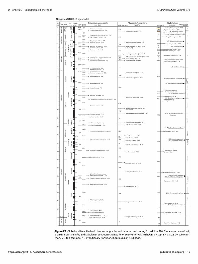
3. Biostratigraphy and paleoenvironmentMicrofossils were examined to provide preliminary shipboard biostratigraphy and paleoenviron-mental information for the recovered sediments. Biostratigraphic age assignments are based on analyses of calcareous nannofossils, planktonic and benthic foraminifers, and radiolarians. Paleodepth interpretations are based on benthic foraminifers. Age assignments are based on the 2012 geological timescale of Gradstein et al. (2012) (GTS2012) (Figure F7). Biohorizons taken from other sources (see below) are recalibrated to the GTS2012. Correlation of New Zealand
.102.2022 publications.iodp.org · 18
U. Röhl et al. · Expedition 378 methods IODP Proceedings Volume 378
https://doi.org/10.14379/iodp.proc.37
Figure F7. Global and New Zealand chronostratigraphy and datums used during Expedition 378. Calcareous nannofossil, planktonic foraminifer, and radiolarian zonation schemes for 0–66 My interval are shown. T = top, B = base, Bc = base com-mon, Tc = top common, X = evolutionary transition. (Continued on next page.)
M9a
C6C
C6B
C6AA
C6A
C6
C5E
C5D
C5C
C5B
C5AB
C5AA
C5A
NN1
NN2
22.82
NN3
NN4
NN5
NN6
19.03
17.95
14.91
13.53
Sphenolithus belemnos
Discoaster druggi (s.s.)
Sphenolithus heteromorphus
Helicosphaera ampliaperta
Sphenolithus belemnos
Triquetrorhabdulus carinatus
Discoaster signus
Sphenolithus heteromorphus
Helicosphaera euphratis --> H. carteri dominance
Sphenolithus disbelemnos
Calcidiscus premacintyrei (Tc)
Sphenolithus delphix
Olig
ocne
Mio
cene
Cha
ttian
Aqui
tani
anBu
rdig
alia
nLa
nghi
anSe
rrava
llian
12
13
14
15
16
17
18
19
20
21
22
23
24
23.0323.06
18.28
Sout
hlan
d
Wai
auan
Lillb
urni
anC
lifde
nian
Pare
ora
Alto
nian
Ota
ian
Land
on
Wai
taki
an
RP22b
RN1
RN2
RN3
RN4
RN5
RP22a
RN6
(Tc) T. carinatus 22.10
CMN9
CMN8
12.57
CMN7
15.73
CMN6
CMN5
CMN4
CMN3
CMN2
CMN1
CMO6
Fohsella robustaFohsella fohsi 13.41
Fohsella"praefohsi" 13.77
Fohsella peripheroacuta 14.24
Orbulina suturalis 15.1
Praeorbulina sicana 16.38
Globigerinatella sp. 19.3
Paragloborotalia kugleri 22.96
Catapsydrax dissimilis 17.54
Paragloborotalia kugleri 21.12
13.13
O7
M1
M2
M3
M4
M5
M6
M7
M8
M9b Diartus petterssoni 12.6
X Dorcadospyris dentata - D. alata 15.03
Calocycletta costata 17.59
Stichocorys wolffii 18.62
Theocyrtis annosa 21.3
Cyrtocapsella tetrapera 22.45
Eucyrtidium diaphanes 3.72
Cycladophora spongothorax12.17
Actinomma golownini13.55
A. g
olow
nini
Cycladophora humerus13.71
C. h
umer
usE
. pun
ctat
um
Eucyrtidium punctatum17.98Cycladophora golli regipileus18.05
C. g
oll.
regi
pile
us
Cyrtocapsella longithorax20.11 C. l
ongi
thor
ax
Cycladophora antiqua21.55
C. a
ntiq
ua
aRP18
Paragloborotalia mayeri/siakensis
Mio
cene
Epoch/Age
Plio
cene
Plei
stoc
ene
Hol
ocen
e
Torto
nian
Mes
sini
anZa
ncle
anPi
acen
zian
Gel
asia
nC
alab
rian
Tarantian
C5
C4A
C4
C3B
C3A
C3
C2A
C2
C1
Ioni
an(m
. Ple
ist.)
Age(Ma)
0
1
2
3
4
5
6
7
8
9
10
11
2.6
5.3W
anga
nui
Haw
eran
Cas
tlecl
iffia
nN
uku-
mar
uan
Man
ga-
pani
anW
aipi
pi-
anO
poita
nKa
pite
an
Tara
naki
Tong
apor
utua
n
Sout
hlan
d
Wai
auan
NZ series/stage
Polaritychron
7.78
3.89
3.49
2.872.74
2.04
1.21
0.59
0.44
0.18
8.39
Buccinosphaera invaginata
Stylatractus universus
Collosphaera tuberosa
Anthocyrtidium angulare
Pterocanium prismatium
Anthocyrtidium jenghisiStichocorys peregrina
Phormostichoartus stula
Phormostichoartus doliolum Didymocyrtis penultima 4.24
X Stichocorys peregrina - S. delmontensis
Diartus hughesi
NN7
NN8
NN9
NN10
NN11
NN12
NN13
NN14NN15
NN16
NN17
NN18
NN19
NN20NN21
10.55
5.12
2.492.39
0.44
9.53
8.29
1.93
1.06
0.29Emiliania huxleyi
Bc Discoaster asymmetricus
Ceratolithus rugosusCeratolithus acutus
Nicklithus amplicus
Amaurolithus spp.
Discoaster berggrenii
Discoaster hamatus
Catinaster coalitus
Bc Discoaster kugleri
Pseudoemiliania lacunosa
Discoaster brouweri
Discoaster pentaradiatusDiscoaster surculus
Discoaster tamalis
Reticulofenestra pseudoumbilicus 3.70Amaurolithus spp.
Discoaster quinqueramus
Nicklithus amplicus
Discoaster hamatus
Gephyrocapsa (>5.5 μm)
Ceratolithus acutus
Tc Discoaster kugleri
1.25
2.80
3.924.04
5.365.53
10.79
11.90
Low latitude
Calcareous nannofossils Planktonic foraminifers RadiolariansWade et al. (2011)
M10
M11
M12
M13b
M14
PL1
PL2PL3
PL4
PL5
PL6
PT1a
PT1b
Globigerinoidesella fistulosa
5.57Globorotalia tumida [Pac.]
8.58Globorotalia plesiotumida
9.83Neogloboquadrina acostaensis
Globorotalia tosaensis
Dentoglobigerina altispira [Pac.]
Sphaeroidinellopsis seminulina [Pac.] 3.85Hirsutella margaritae
Globoturborotalita nepenthes
10.46
11.79Fohsella fohsi lobata
0.61
1.93
3.59
M13a
RN7
RN8
RN9
RN10
RN11a
RN11b
RN12a
RN12b
RN13
RN14
RN15RN16
RN17
8.84X Diartus petterssoni - D. hughesi
Ω
Stylatractus universus0.46
Pterocanium charybdeum trilobum0.59
Ψ
χ
Eucyrtidium calvertense1.73
Helotholus vema2.35
Φ
Helotholus vema4.88
Υ
Amphymenium challengerae6.22
Τ
Amphymenium challengerae6.84 A. c
halle
n-ge
rae
Acrosphaera(?) labrata7.84
A.?
labr
ata
Cycladophora spongothorax8.62 S. v
esuv
ius
X Acrosphaera murrayana- A. australia
10.45
A. a
ustra
lisC
. spo
ngot
hora
x
Menardella pseudomiocenica 2.39[Indo-Pacific]
3.47
[(sub)tropical]
Globorotalia lenguaensis 6.09
11.63Globoturborotalia nepenthes
CNPL11
T absence Gephyrocapsa (>4 μm)
CNPL10
CNPL9
Gephyrocapsa (>4 μm) 1.71CNPL8
CNPL7
CNPL6
CNPL5
CNPL4
CNPL3
5.04
CNPL2
CNPL1
CNM20
CNM19
5.98
6.82
CNM18
7.39CNM17
CNM16
CNM15
CNM14
B absence Reticulofenestra pseudoumbilicus 8.8
CNM13
CNM12
11.6
CNM11
CNM10
C5AC
C5AD
Martini (1971)
Agnini et al. (2014)
Neogene (GTS2012 age model)
Southwest Pacific(Zealandia)Age (Ma) Age (Ma) Age (Ma)
8.102.2022 publications.iodp.org · 19

U. Röhl et al. · Expedition 378 methods IODP Proceedings Volume 378
https://doi.org/10.14379/iodp.proc.378
stages with the GTS2012 is based on Raine et al. (2015). Biohorizons are listed in Tables T2 (cal-careous nannofossils), T3 (foraminifers), and T4 (radiolarians). Taxonomic lists for key species in these three groups are provided in Tables T5, T6, and T7.
Microfossil samples were collected from almost all core catcher sections, and additional samples, mostly for nannofossil biostratigraphy, were taken from working-half sections to refine age estimates and to initially constrain critical intervals. Where necessary, sample depths are cited as sample intervals. Biohorizon depths are generally cited as the midpoint between the two samples bounding the biohorizon. For the purposes of shipboard age estimation, emphasis was placed on age diagnostic species and total assemblages were not completely described. Information on microfossil group preservation, abundance, taxon identifications, and zonal assignment were uploaded into the LIMS database through DESClogik.
Figure F7 (continued).
E7b
E7a
P1b
P2
P3a
P4b
P1c
P1a
P3b
P4c
P4a
Theocyrtis tuberosa
Age(Ma) Epoch/Age
Eoce
neO
ligoc
ene
Neogene
Polaritychron
25
30
35
40
Lute
tian
Pria
boni
anBa
rtoni
anR
upel
ian
Cha
ttian
C20
C19
C18
C17
C16
C15
C13
C12
C11
C10
C9
C8
C7A
C7
C6C
C6B
NP16
NP17
NP18
NP19-NP20
NP21
NP22
NP23
NP24
NP25
NN1
NN2
(>10 μm)
(base of acme)
Chiasmolithus solitus
22.8223.13
26.84
29.62
30.00
32.02
32.92
40.40
34.44
43.59NP15c
33.87
24.43
26.93
23.03
33.89
Chiasmolithus gigas
Wai
taki
anD
untro
onia
nW
hain
garo
anR
unan
gan
Kaia
tan
Land
onAr
nold
Borto
nian
Pora
ngan
Discoaster druggiReticulofenestra bisectus
Sphenolithus ciperoensis
Sphenolithus distentusSphenolithus predistentus
Sphenolithus ciperoensis
Sphenolithus distentus
Reticulofenestra umbilicus
Coccolithus formosus
Clausicoccus subdistichus
Discoaster saipanensis
Cretaceous
Pale
ocen
e
Dan
ian
Sela
ndia
nTh
anet
ian
Ypre
sian
C29
C28
C27
C26
C25
C24
C23
C22
C21
C20
NP1
NP2
NP3
NP4
NP5
NP6NP7
NP8
NP10
NP11
NP12
NP13
NP14
Nannotetrina alata group/N. fulgens
Discoaster sublodoensis (Bc)(5-rayed)
Discoaster lodoensis
Tribrachiatus orthostylus
Tribrachiatus bramlettei
Discoaster backmanii
Discoaster multiradiatus
Heliolithus riedeliiDiscoaster mohleriHeliolithus kleinpellii
Fasciculithus tympaniformisFasciculithus 2nd radiation = B F. ulii
Ellipsolithus macellus
Chiasmolithus danicus
Cruciplacolithus intermediusBiantholithus sparsusBase acme calcispheres
Tribrachiatus orthostylus
Tribrachiatus contortus
Micula murus, Cretaceous nannofossils
45
50
55
60
65
46.29
49.11
53.70
55.86
58.2858.7058.9759.54
61.51
63.25
64.81
65.4766.04
61.61
57.21NP9
47.73Nannotetrina cristata
NP15a 45.49
NP15b
54.1754.37
55.96
66.04
Chiasmolithus gigas
Sphenolithus moriformis group 62.04
Prinsius martinii
Prinsius dimorphosus group (Bc) 65.28
63.62
Reticulofenestra/Dictyococcites(abundance turnover) 50.50
Fasciculithus spp. 55.64
Dan
nevi
rke
Her
etau
ngan
Man
gaor
apan
Wai
paw
anTe
uria
n
Low latitude
Eusyringium fistuligerum 42.85
Zealithapium mitra39.5
Eucyrtidium spinosum38.15
zRP14
zRP13
zRP12
zRP11
Clinorhabdus robusta28.2
zRP17
Axoprunum(?) irregularis26.12
Unz
oned
Eucyrtidium antiquum33.5
Lychnocanium conicum29.52
zRP16
zRP15
Lychnocanium elongata
Dorcadospyris ateuchus
X Lithocyclia angusta
Calocyclas bandyca
Cryptocarpium azyx
Podocyrtis goetheana
Tristylospyris triceros
Lithocyclia aristotelis gr.
29.23
33.78
37.05
38.26
39.97
41.22
43.17RP13
RP14
RP12
Lophocyrtis hadra 35.70
RP22b
RP21b
RP21a
Lychnocanium apodora
RP20c
RP20b
RP20a
Eucyrtidium plesiodiaphanes
RP19
RP18
RP17
RP16
RP15
RN1
Eucyrtidium diaphanes
RP22a
31.22
32.99
23.72
X Podocyrtis mitra - P. chalara
X Podocyrtis sinuosa - P. mitra
Cyrtocapsella tetrapera 22.45
Eusyringium lagena
Theocampe mongolfieri
X Theocotyle nigriniae - T. cryptocephala
Theocorys anaclasta clasta
Buryella clinata
X Bekoma campechensis - B. bidartensis
Stylotrochus nitidus or Pterocodon(?) poculum
Peritiviator(?) dumitricai
RP9
RP12
RP11
RP10
zRP10
Podocyrtis papalis
zRP9
zRP8
zRP7
Phormocyrtis striata exquisita
Bekoma pentadica60.5
Buryella tetradica
zRP5
zRP6
Buryella foremanae
zRP4
zRP3
zRP2
zRP1
Lychnocanium auxilla
Unzoned
Buryella tetradica51.0
RP8
RP7
RP6c
RP6b
RP6a
E9
E10
E11
E12
E13
E14
E15
E16
O1
O2
O3
O4
O5
O6
O7
M1a
b
Paragloborotalia pseudokugleri
Ciperoella angulisuturalis
Orbulinoides beckmanni
Paragloborotalia opima s.s.
Turborotalia ampliapertura
Pseudohastigerina naguewichiensis
Globigerinatheka index
Orbulinoides beckmanni
Guembelitrioides nuttalli
Morozovelloides crassatus
Globigerinatheka index
25.21
26.93
29.18
30.28
32.1
34.61
40.0340.49
42.07
42.6
38.25
39.1
P0Pα
P5
E1E2
E3
E4
E5
E6
E8
Globanomalina pseudomenardii
Globanomalina pseudomenardii
Morozovella formosa
57.1
60.73
Guembelitrioides nuttalli 45.72
54.61
Acarinina cuneicamerata 50.2
NZ series/stage
Calcareous nannofossils Planktonic foraminifers Radiolarians
Nannotetrina alata group/N. fulgens 42.87
Fasciculithus reinhardii group 56.00
Heliolithus cantabriae 59.54
Bc Toweius pertusus (circular) 63.12
CNP1CNP2
CNP3
CNP4
CNP5
CNP6
CNP7
CNP8
CNP9
CNP10
CNP11
CNE1
CNE2
CNE3
CNE4
CNE5
CNE7
CNE8
CNE10
CNE11
CNE12
CNE13
CNE14
CNE15
CNE17
CNE18
CNE19
CNE20
CNE21
CNO1
CNO2
CNO3
CNO4
CNO5
CNO6
Martini (1971)
Agnini et al. (2014)
25.21
26.5
43.81X Podocyrtis phyxis - P.ampla
45.24
47.40
50.05Theocampe mongolfieri50.0
53.35
58.2359.0
60.4
Bekoma campechensis 61.5
62.4
64.0
Buryella granulata64.9
Amphisphaera kina65.5Amphisphaera aotea66.04
55.96
57.5
54.1
48.57
Paragloborotalia kugleri 22.96
AO4
Globigerina labiacrassata26.5
AO3
Chiloguembelina cubensis Tc28.1Tc Chiloguembelina cubensis 28.09
Subbotina angiporoides29.80
AO2
Hantkenina spp., Hantkenina alabamensis 33.89
AO1
Globigerinatheka index34.6
AE9Tenuitella insolita35.7
Globigerinatheka semiinvoluta 36.18
AE8
Acarinina primitiva
Subbotina agiporoides42.11
AE7
AE6
Morozovella aragonensis 43.26
Globigerinatheka kugleri 43.26 AE5
Cassigerinelloita amekiensis46.13
Turborotalia frontosa 48.31 AE4
Cassigerinelloita amekiensis50.04
Morozovella subbotinae 50.67
Acarinina primitiva51.43
AE3
Morozovella aragonensis 52.54 AE2
Chiloguembelina wilcoxensis53.94
Morozovella velascoensis 55.2Pseudohastigerina wilcoxensis 55.81
AE1
Globanomalina australiformis55.96Acarinina sibaiyaensis 55.96
Subbotina triloculinoides57.64
AP4
Acarinina soldadoensis 57.79
Parasubbotina variospira 60.52
AP3
Acarinina subsphaerica60.52
Igorina albeari 61.33 AP2
Globoconusa daubjergensis62.23Morozovella angulata 62.29Praemurica uncinata 62.6 AP1c
Globanomalina compressa63.9
Praemurica inconstans63.9
AP1b
Subbotina triloculinoides65.52AP1a
Globoconusa daubjergensis65.72
Subbotina triloculinoides 65.25
Parvularugoglobigerina eugubina 65.72Parvularugoglobigerina eugubina 66.0
Wade et al. (2011)Austral Realm
Huber & Quillevere (2005)Southern Ocean
Fioroni et al. (2012)
D. bisectus
R. daviesii
B. spinosus
C. altus
R. samodurovi
R. oamaruensis
I. recurvus
C. o
amar
uens
isZ. bijugatus
N. dubius
C. oamaruensis/C. solitus
E. formosa
C. reticulatum/R. clatrata
S. moriformis
C. expansus
C. r
etic
ulat
um/E
. for
mos
a
R. umbilicus
Chiasmolithus altus25.58
Reticulofenestra umbilicus (Tc)31.51
Isthmolithus recurvus32.49
Chiasmolithus altus32.49
Reticulofenestra oamaruensis33.97
Isthmolithus recurvus (Bc)36.01Reticulofenestra oamaruensis35.54
Neococcolithus dubius36.70
Chiasmolithus solitus38.34CNE16
Bc Sphenolithus cuniculus 44.64
CNE9
CNE6Discoaster sublodoensis 48.37
Chiasmolithus oamaruensis38.80
Coccolithus formosus (Tc)39.02Discoaster spp. (Tc)40.08
Reticulofenestra clatrata40.56Reticulofenestra reticulata40.69
Reticulofenestra umbilicus42.48
Unz
oned
Paleogene (GTS2012 age model)
Southwest Pacific(Zealandia)Age (Ma) Age (Ma) Age (Ma)
37.98 Isthmolithus recurvus
Reticulofenestra reticulata 41.66
.102.2022 publications.iodp.org · 20

U. Röhl et al. · Expedition 378 methods IODP Proceedings Volume 378
Table T2. Biochronology of calcareous nannofossil datum events, Expedition 378. B = base (lowest occurrence), T = top (highest occurrence), Tc = highest common occurrence, Bc = lowest common occurrence, X = crossover of dominance. (Continued on next two pages.) Download table in CSV format.
Zone/subzone base
BiohorizonGTS 2012
(Ma)Calibration reference
Low-latitude zonations (Martini, 1971)
Low-latitude zonations (Backman et al., 2012)
Southern Ocean zonation(Fioroni et al., 2012)
NN21CNPL11
B Emiliania huxleyi 0.29 Lourens et al., 2005 NN20 T Pseudoemiliania lacunosa 0.44 Lourens et al., 2005
NN19
CNPL10Tc Reticulofenestra asanoi 0.91 Lourens et al., 2005T absence Gephyrocapsa (≥4 μm) 1.06 Backman et al., 2012
CNPL9Bc Reticulofenestra asanoi 1.14 Lourens et al., 2005T Gephyrocapsa (>5.5 μm) 1.25 Lourens et al., 2005
CNPL8
T Helicosphaera sellii 1.26 Lourens et al., 2005B Gephyrocapsa (>5.5 μm) 1.62 Lourens et al., 2005T Calcidiscus macintyrei 1.60 Lourens et al., 2005B Gephyrocapsa (≥4 μm) 1.71 Lourens et al., 2005
CNPL7 T Discoaster brouweri 1.93 Lourens et al., 2005
NN18 CNPL6Bc Discoaster triradiatus 1.95 Lourens et al., 2005T Discoaster pentaradiatus 2.39 Lourens et al., 2005
NN17CNPL5
T Discoaster surculus 2.49 Lourens et al., 2005
NN16
Pliocene/Pleistocene boundary 2.59T Discoaster tamalis 2.76 Backman et al., 2012
CNPL4T Sphenolithus spp. 3.61 Backman et al., 2012T Reticulofenestra pseudoumbilicus 3.82 Backman et al., 2012
NN15CNPL3
T Amaurolithus spp. 3.92 Gradstein et al., 2012NN14 Bc Discoaster asymmetricus 4.04 Backman et al., 2012
NN13CNPL2 T Ceratolithus acutus 5.04 Lourens et al., 2005
CNPL1
B Ceratolithus rugosus 5.12 Lourens et al., 2005
NN12
T Triquetrorhabdulus rugosus 5.28 Lourens et al., 2005Miocene/Pliocene boundary 5.33B Ceratolithus acutus 5.36 Lourens et al., 2005
CNM20 T Discoaster quinqueramus 5.53 Backman et al., 2012
NN11
CNM19 T Nicklithus amplificus 5.98 Backman et al., 2012CNM18 B Nicklithus amplificus 6.82 Backman et al., 2012
CNM17T absence Reticulofenestra pseudoumbilicus 7.09 Backman et al., 2012B Amaurolithus spp. 7.39 Backman et al., 2012
CNM16 B Discoaster berggrenii 8.29 Backman et al., 2012
NN10CNM15 B absence Reticulofenestra pseudoumbilicus 8.80 Backman et al., 2012CNM14 T Discoaster hamatus 9.53 Backman et al., 2012
NN9 CNM13 B Discoaster hamatus 10.55 Lourens et al., 2005
NN8 CNM12T Coccolithus miopelagicus 10.97 Raffi et al., 2006B Catinaster coalitus 10.79 Lourens et al., 2005
NN7CNM11 Tc Discoaster kugleri 11.60 Backman et al., 2012CNM10 Bc Discoaster kugleri 11.88 Backman et al., 2012
NN6CNM9 Tc Calcidiscus premacintyrei 12.57 Backman et al., 2012CNM8 T Sphenolithus heteromorphus 13.53 Lourens et al., 2005
NN5 T Helicosphaera ampliaperta 14.91 Lourens et al., 2005
NN4CNM7
Tc Discoaster deflandrei 15.69 Backman et al., 2012B Discoaster petaliformis (= D. signus) 15.73 Backman et al., 2012
CNM6 B Sphenolithus heteromorphus 17.75 Lourens et al., 2005
CNM5T Sphenolithus belemnos 17.96 Lourens et al., 2005
NN3 T Triquetrorhabdulus carinatus 18.28 Lourens et al., 2005
NN2
B Sphenolithus belemnos 19.01 Lourens et al., 2005
CNM4B Helicosphaera ampliaperta 20.43 Lourens et al., 2005X Helicosphaera euphratis/H. carteri 20.89 Backman et al., 2012
CNM3 Tc Triquetrorhabdulus carinatus 22.10 Backman et al., 2012CNM20 B Sphenolithus disbelemnos 22.41 Backman et al., 2012
CNM1
B Discoaster druggii 22.59 Backman et al., 2012
NN1
T Sphenolithus capricornutus 22.97 Gradstein et al., 2012Oligocene/Miocene boundary 23.03 Lourens et al., 2005T Sphenolithus delphix 23.06 Backman et al., 2012
CNO6B Sphenolithus delphix 23.38 Backman et al., 2012
Dictyococcites bisectus (R. bisecta)
T Sphenolithus ciperoensis 24.36 Backman et al., 2012
NP25CNO5
X Triquetrorhabdulus longus/T. carinatus 25.04 Backman et al., 2012T Chiasmolithus altus 25.58 Fioroni et al., 2012
Chiasmolithus altus
T Sphenolithus distentus 26.84 Blaj et al., 2009
NP24T Sphenolithus predistentus 26.93 Blaj et al., 2009
CNO4B Sphenolithus ciperoensis 29.62 Agnini et al., 2014
NP23B Sphenolithus distentus 30.00 Blaj et al., 2009
CNO3Tc Reticulofenestra umbilicus (>14 μm) (high Lat) 31.51 Fioroni et al., 2012
Reticulofenestra daviesiiT Reticulofenestra umbilicus (>14 μm) 32.02 Blaj et al., 2009
NP22 CNO2 T Isthmolithus recurvus (high Lat) 32.49 Fioroni et al., 2012
https://doi.org/10.14379/iodp.proc.378.102.2022 publications.iodp.org · 21

U. Röhl et al. · Expedition 378 methods IODP Proceedings Volume 378
NP22 CNO2Blackites spinosus
T Coccolithus formosus 32.92 Blaj et al., 2009T Isthmolithus recurvus 32.99 Villa et al., 2008
NP21
CNO1B Chiasmolithus altus 33.31 Fioroni et al., 2012
Reticulofenestra samodurovi
Ba Reticulofenestra daviesii 33.71 Fioroni et al., 2012Bc Clausicoccus subdistichus 33.88 Agnini et al., 2014
CNE21Eocene/Oligocene boundary 33.89T Reticulofenestra oamaruensis 33.97 Fioroni et al., 2012
Reticulofenestra oamaruensis
T Discoaster saipanensis 34.44 Blaj et al., 2009
NP19/NP20
CNE20T Discoaster barbadiensis 34.77 Blaj et al., 2009T Reticulofenestra reticulata 35.23 Agnini et al., 2014
CNE19
B Reticulofenestra oamaruensis 35.54 Fioroni et al., 2012
Isthmolithus recurvusT Reticulofenestra reticulata (high Lat) 35.92 Villa et al., 2008Bc Isthmolithus recurvus (high Lat) 36.01 Fioroni et al., 2012
Zygrablithus bijugatus (subzone)
B Reticulofenestra isabellae 36.30 Agnini et al., 2014
CNE18T Neococcolithus dubius 36.70 Fioroni et al., 2012
Neococcolithus dubius (subzone)
Bc Isthmolithus recurvus 36.97 Fornaciari et al., 2010
NP18B Isthmolithus recurvus (high Lat) 37.98 Fioroni et al., 2012
CNE17T Chiasmolithus grandis 37.98 Agnini et al., 2014B Chiasmolithus oamaruensis 38.03 Agnini et al., 2014
NP17
Bc Reticulofenestra erbae 38.06 Fornaciari et al., 2010
CNE16T Chiasmolithus solitus 38.34 Fioroni et al., 2012
C. oamaruensis/C. solitus (subzone)
T Sphenolithus obtusus 38.65 Fornaciari et al., 2010
CNE15
B Chiasmolithus oamaruensis (high Lat) 38.80 Fioroni et al., 2012Ericsonia formosa Tc Coccolithus formosus 39.02 Fioroni et al., 2012
Sphenolithus moriformis (subzone)
Tc Sphenolithus spiniger 39.70 Fornaciari et al., 2010B Sphenolithus obtusus 39.70 Fornaciari et al., 2010Tc Discoaster spp. 40.08 Fioroni et al., 2012
Chiasmolithus expansus (subzone)
B Reticulofenestra bisecta (high Lat) 40.12 Fioroni et al., 2012B Reticulofenestra bisecta (>10 μm) 40.36 Agnini et al., 2014
CNE14
T Chiasmolithus solitus (mid-low Lat) 40.40 Berggren et al., 1995 T Sphenolithus furcatolithoides morphotype B 40.48 Agnini et al., 2014
NP16
T Reticulofenestra clatrata 40.56 Fioroni et al., 2012Cribrocentrum retic. [R. retic.]/ R. cla.
(subzone)B Reticulofenestra reticulata (high Lat) 40.69 Fioroni et al., 2012
Reticulofenestra umbilicus
Bc Reticulofenestra reticulata 41.66 Agnini et al., 2014
CNE13T Nannotetrina spp. 41.85 Agnini et al., 2014T Nannotetrina alata gr. 42.87 Backman, 1986Bc Reticulofenestra umbilicus 41.94 Agnini et al., 2014
CNE12
B Reticulofenestra umbilicus (high Lat) 42.48 Fioroni et al., 2012
NP15cT Nannotetrina fulgens 42.87 Gradstein et al., 2012B Sphenolithus furcatolithoides morphotype B 43.48 Agnini et al., 2014T Chiasmolithus gigas 45.49 Agnini et al., 2014
NP15bCNE11 Bc Sphenolithus cuniculus 44.21 Agnini et al., 2014
CNE10B Sphenolithus furcatolithoides morphotype A 45.42 Agnini et al., 2014B Chiasmolithus gigas 45.49 Agnini et al., 2006
NP15a CNE9 B Nannotetrina alata gr. 46.29 Agnini et al., 2006
NP14
CNE8 B Nannotetrina cristata 47.73 Agnini et al., 2006CNE7 T Discoaster lodoensis 47.41 Agnini et al., 2006
CNE6B Blackites inflatus 47.84 Gradstein et al., 2012Bc Discoaster sublodoensis (5-rayed) 49.11 Agnini et al., 2006
NP13CNE5 T Tribrachiatus orthostylus 50.50 Agnini et al., 2006
CNE4X Dictyococcites/Reticulofenestra 50.50 Agnini et al., 2006
NP12B Coccolithus crassus 50.82 Agnini et al., 2014B Discoaster lodoensis 53.70 Agnini et al., 2007
NP11CNE3
B Toweius gammation 53.78 Agnini et al., 2016T Tribrachiatus contortus 54.17 Agnini et al., 2007
NP10
B Sphenolithus radians 54.17 Agnini et al., 2007B Tribrachiatus orthostylus 54.37 Agnini et al., 2007
CNE2B Discoaster diastypus 54.95 Agnini et al., 2007T Fasciculithus tympaniformis (= Fasciculithus spp). 55.64 Agnini et al., 2007
CNE1
B Tribrachiatus bramlettei 55.86 Agnini et al., 2007
NP9
B Rhomboaster spp. 55.96 Agnini et al., 2007Paleocene/Eocene boundary 55.96T Fasciculithus richardii group 56.00 Agnini et al., 2007
CNP11T Ericsonia robusta (>9 μm) 56.68 Agnini et al., 2007B Discoaster multiradiatus 57.10 Agnini et al., 2007
Zone/subzone base
BiohorizonGTS 2012
(Ma)Calibration reference
Low-latitude zonations (Martini, 1971)
Low-latitude zonations (Backman et al., 2012)
Southern Ocean zonation(Fioroni et al., 2012)
Table T2 (continued). (Continued on next page.)
https://doi.org/10.14379/iodp.proc.378.102.2022 publications.iodp.org · 22

U. Röhl et al. · Expedition 378 methods IODP Proceedings Volume 378
NP8CNP10
Tc Sphenolithus anarrhopus 57.26 Gradstein et al., 2012B Discoaster okadai 57.35 Agnini et al., 2007B Discoaster delicatus 57.45 Agnini et al., 2007B Ericsonia robusta (>9 μm) 57.54 Agnini et al., 2007B Discoaster nobilis 57.50 Agnini et al., 2007Tc Discoaster backmanii 57.57 Agnini et al., 2007B Discoaster backmanii 58.28 Gradstein et al., 2012
CNP9B Heliolithus riedelii 58.70 Agnini et al., 2007
NP7B Discoaster mohleri 58.97 Agnini et al., 2007
CNP8B Sphenolithus anarrhopus 59.40 Agnini et al., 2007
NP6B Heliolithus kleinpellii 59.54 Agnini et al., 2007B Heliolithus cantabriae 59.60 Agnini et al., 2007
NP5
CNP7B Fasciculithus tympaniformis 61.51 Agnini et al., 2007B Fasciculithus second radiation = B F. ulii 61.61 Agnini et al., 2007
CNP6B Neochiastozygus perfectus 61.76 Agnini et al., 2007B Sphenolithus moriformis gr. 62.04 Agnini et al., 2014
CNP5B Chiasmolithus bidens/edentulus 62.07 Gradstein et al., 2012B Fasciculithus first radiation 62.13 Gradstein et al., 2012Bc Toweius pertusus (circular) 63.12 Agnini et al., 2014
NP4 CNP4B Ellipsolithus macellus 63.25 Gradstein et al., 2012B Prinsius martinii 63.62 Agnini et al., 2014
NP3CNP3
B Chiasmolithus danicus 64.81 Gradstein et al., 2012Bc Praeprinsius dimorphosus gr. 65.28 Agnini et al., 2014
CNP2B Cruciplacolithus tenuis 65.47 Gradstein et al., 2012
NP2
B Cruciplacolithus intermedius 65.47 Gradstein et al., 2012B Coccolithus pelagicus 65.70 Agnini et al., 2014
CNP1
B Cruciplacolithus primus (3.5–5 μm) 65.76 Gradstein et al., 2012B Neobiscutum parvulum 65.90 Gradstein et al., 2012
NP1
B Biantholithus sparsus, Ba Calcispheres 66.04 Gradstein et al., 2012Cretaceous/Paleogene boundary 66.04T Cretaceous nannoflora 66.04 Agnini et al., 2014B Micula prinsii 67.30 Gradstein et al., 2012
NC23B Nephrolithus frequens 67.84 Gradstein et al., 2012B Micula murus 69.00 Gradstein et al., 2012
NC22B Lithraphidites quadratus 69.18 Gradstein et al., 2012T Reinhardtites levis 70.14 Gradstein et al., 2012T Tranolithus orionatus 71.01 Gradstein et al., 2012
NC21 T Uniplanarius trifidus 71.31 Gradstein et al., 2012
Zone/subzone base
BiohorizonGTS 2012
(Ma)Calibration reference
Low-latitude zonations (Martini, 1971)
Low-latitude zonations (Backman et al., 2012)
Southern Ocean zonation(Fioroni et al., 2012)
Table T2 (continued).
Biostratigraphic analyses were carried out for all holes drilled at Site U1553. Datum tables, micro-fossil distribution charts, an integrated biozonation figure, and a microfossil group abundance and preservation figure are included in Biostratigraphy and micropaleontology in the Site U1553 chapter (Röhl et al., 2022a).
3.1. Calcareous nannofossils
3.1.1. Taxonomy and biostratigraphyNannofossil taxonomy refers to Bown (1998, 2005) and Perch-Nielsen (1985a, 1985b) as compiled in the online Nannotax3 database (http://www.mikrotax.org/Nannotax3). The nannofossil biohorizons used for biostratigraphic classification (Table T2) represent an integration of the zonal scheme of Martini (1971; zonal codes NP and NN) with the Southern Ocean calcareous nan-nofossil zonal scheme of Fioroni et al. (2012) used for the Oligocene to upper Eocene interval. Additional biohorizons from the Paleogene and Neogene biozonation schemes of Agnini et al. (2014; zonal codes CNP, CNE, and CNO) and Backman et al. (2012; CNM and CNPL) are also included, although they are based predominantly on mid- to low-latitude calcareous nannofossil assemblages. This composite zonation scheme provides a general framework for calcareous nan-nofossil biostratigraphic classification (Figure F7).
https://doi.org/10.14379/iodp.proc.378.102.2022 publications.iodp.org · 23

U. Röhl et al. · Expedition 378 methods IODP Proceedings Volume 378
https://doi.org/10.14379/iodp.proc.378.1
Table T3. Biochronology of planktonic foraminiferal datum events, Expedition 378. * = benthic foraminifer. B = bottom (lowest occurrence), T = top (highest occurrence), HCO = highest common occurrence. Parentheses indicate estimated ages at high latitudes. (Continued on next page.) Download table in CSV format.
Tropical zone/subzone
base EventGTS 2012 age (Ma) Calibration reference
PL6 B Truncorotalia crassula 2.40 Raine et al., 2015Miocene/Oligocene boundary 23.03 Gradstein et al., 2012
M1a T Globoturborotalita euapertura 23.03 Gradstein et al., 2012T Tenuitella gemma 23.50 Raine et al., 2015T common Trilobatus primordius 23.50 Gradstein et al., 2012B Globoturborotalita woodi ~24.0 Crundwell et al., 2016 B Globoquadrina dehiscens 25.20 Gradstein et al., 2012
O7 B Paragloborotalia pseudokugleri 25.21 Gradstein et al., 2012AO4 T Globoturborotalita labiacrassata 26.50 Gradstein et al., 2012
B Trilobatus primordius 26.12 Raine et al., 2015O6 T Paragloborotalia opima s.s. 26.93 Gradstein et al., 2012
B Notorotalia spinosa* 27.30 Gradstein et al., 2012AO3 T Chiloguembelina cubensis (HCO) 28.10 Gradstein et al., 2012O5 T common Chiloguembelina cubensis 28.09 Gradstein et al., 2012O4 B Ciperoella angulisuturalis 29.18 Raine et al., 2015
B Globigerina juvenilis 29.50 Gradstein et al., 2012AO2 T Subbotina angiporoides 29.80 Gradstein et al., 2012
T Subbotina angiporoides 29.84 Gradstein et al., 2012O3 T Turborotalia ampliapertura 30.28 Gradstein et al., 2012
B Paragloborotalia opima 30.72 Gradstein et al., 2012O2 T Pseudohastigerina naguewichiensis 32.10 Gradstein et al., 2012
B Cassigerinella chipolensis 33.89 Gradstein et al., 2012Oligocene/Eocene boundary 33.89 Gradstein et al., 2012
O1 T Hantkenina spp., H. alabamensis 33.89 Gradstein et al., 2012T common Pseudohastigerina micra 33.89 Gradstein et al., 2012T Turborotalia cerroazulensis 34.03 Raine et al., 2015T Cribrohantkenina inflata 34.22 Gradstein et al., 2012
AO1 T Globigerinatheka index 34.60 Gradstein et al., 2012E16 T Globigerinatheka index 34.60 Gradstein et al., 2012AE10 T Tenuitella insolita 34.75 Gradstein et al., 2012
T Turborotalia pomeroli 35.66 Gradstein et al., 2012AE9 B Tenuitella insolita 35.70 Gradstein et al., 2012
B Turborotalia cunialensis 35.71 Gradstein et al., 2012B Cribrohantkenina inflata 35.87 Raine et al., 2015
E15 T Globigerinatheka semiinvoluta 36.18 Gradstein et al., 2012B Bolivina pontis* 36.70 Gradstein et al., 2012T Acarinina spp. 37.75 Gradstein et al., 2012T Subbotina linaperta 37.96 Gradstein et al., 2012T Acarinina collactea 37.96 Gradstein et al., 2012
E14 T Morozovelloides crassatus 38.25 Gradstein et al., 2012B Globigerinatheka semiinvoluta 38.62 Gradstein et al., 2012T Acarinina mcgowrani 38.62 Raine et al., 2015T Planorotalites spp. 38.62 Gradstein et al., 2012
AE8 T Acarinina primitiva 39.10 Gradstein et al., 2012T Acarinina primitiva 39.12 Gradstein et al., 2012T Turborotalia frontosa 39.42 Gradstein et al., 2012
E13 T Orbulinoides beckmanni 40.03 Gradstein et al., 2012E12 B Orbulinoides beckmanni 40.49 Gradstein et al., 2012
T Acarinina bullbrooki 40.49 Gradstein et al., 2012E11 T Guembelitrioides nuttalli (42.07) Gradstein et al., 2012AE7 B Subbotina angiporoides 42.11 Gradstein et al., 2012
B Turborotalia pomeroli 42.21 Gradstein et al., 2012AE6 B Globigerinatheka index 42.60 Gradstein et al., 2012
B Globigerinatheka index 42.64 Gradstein et al., 2012B Morozovelloides lehneri 43.15 Gradstein et al., 2012
E10 T Morozovella aragonensis 43.26 Gradstein et al., 2012E9 B Globigerinatheka kugleri (43.88) Raine et al., 2015
T Morozovella crater 45.70 Raine et al., 2015B Elphidium saginatum* 45.70 Gradstein et al., 2012B Hantkenina singanoae (44.49) Gradstein et al., 2012B Turborotalia possagnoensis 45.49 Gradstein et al., 2012
E8 B Guembelitrioides nuttalli (45.72) Gradstein et al., 2012AE5 T Cassigerinelloita amekiensis 46.13 Gradstein et al., 2012E7b B Turborotalia frontosa 48.31 Raine et al., 2015
T Morozovella dolobrata 48.60 Dallanave et al., 2015 B Elphidium hampdenense* 48.90 Gradstein et al., 2012
AE4 B Cassigerinelloita amekiensis 50.04 Gradstein et al., 2012
02.2022 publications.iodp.org · 24

U. Röhl et al. · Expedition 378 methods IODP Proceedings Volume 378
https://doi.org/10.14379/iodp.proc.378
E7a B Acarinina cuneicamerata 50.20 Gradstein et al., 2012B Planorotalites palmerae 50.20 Gradstein et al., 2012
E6 T Morozovella subbotinae 50.67 Gradstein et al., 2012B Acarinina pentacamerata 50.67 Gradstein et al., 2012
AE3 B Acarinina primitiva 51.43 Gradstein et al., 2012B Morozovella crater 52.00 Raine et al., 2015T Morozovella aequa aequa 52.50 Dallanave et al., 2015
E5 B Morozovella aragonensis 52.54 Gradstein et al., 2012T Morozovella marginodentata 52.85 Gradstein et al., 2012T Morozovella lensiformis 53.14 Gradstein et al., 2012
AE2 T Chiloguembelina wilcoxensis 53.94 Gradstein et al., 2012T Morozovella aequa 54.20 Gradstein et al., 2012
E4 B Morozovella formosa 54.61 Gradstein et al., 2012B Morozovella lensiformis 54.61 Gradstein et al., 2012B Morozovella lensiformis 55.00 Dallanave et al., 2015T Subbotina velascoensis 55.07 Gradstein et al., 2012
E3 T Morozovella velascoensis (55.20) Gradstein et al., 2012T Morozovella acuta 55.39 Gradstein et al., 2012B Morozovella gracilis 55.39 Gradstein et al., 2012B Igorina broedermanni 55.39 Gradstein et al., 2012B Morozovella marginodentata 55.54 Gradstein et al., 2012
E2 B Pseudohastigerina wilcoxensis 55.81 Gradstein et al., 2012AE1 B Globanomalina australiformis 55.96 Raine et al., 2015E1 B Acarinina sibaiyaensis 55.96 Gradstein et al., 2012
B Acarinina coalingensis 55.96 Dallanave et al., 2015B Morozovella aequa aequa 55.96 Raine et al., 2015Eocene/Paleocene boundary 55.96 Gradstein et al., 2012
P5 T Globanomalina pseudomenardii 57.10 Gradstein et al., 2012B Morozovella subbotinae 57.10 Gradstein et al., 2012
AP4 T Subbotina triloculinoides 57.64 Gradstein et al., 2012Pα B Parvularugoglobigerina eugubina 66.00 Gradstein et al., 2012
Cretaceous/Paleogene boundary 66.04 Gradstein et al., 2012
Tropical zone/subzone
base EventGTS 2012 age (Ma) Calibration reference
Table T3 (continued).
Table T4. Biochronology of radiolarian datum events, Expedition 378. T = top (highest occurrence), B = bottom (lowest occurrence), Bc = lowest common occurrence, Tc = highest common occurrence, X = crossover of dominance, NC = no calibration available. (Continued on next two pages.) Download table in CSV format.
Zone/subzone base Southern Ocean/Southwest Pacific Ocean
GTS 2012 age (Ma) Callibration reference
Omega W T Stylatractus universus 0.46 McKay et al., 2019Psi Y T Pterocanium charybdeum trilobum 0.59 McKay et al., 2019
T Antarctissa cylindrica 0.65 McKay et al., 2019T Cycladophora pliocenica 1.72 McKay et al., 2019
Chi C T Eucyrtidium calvertense 1.73 McKay et al., 2019B Triceraspyris antarctica 1.88 McKay et al., 2019B Pterocanium charybdeum trilobum 2.24 McKay et al., 2019
Phi F T Helotholus vema 2.35 McKay et al., 2019T Desmospyris spongiosa 2.47 McKay et al., 2019B Cycladophora davisiana 2.51 McKay et al., 2019T Larcopyle polyacantha titan 3.53 McKay et al., 2019T Lampromitra coronata 3.72 McKay et al., 2019T Lychnocanoma grande 4.55 McKay et al., 2019T Eucyrtidium pseudoinflatum 4.6 McKay et al., 2019
Upsilon U B Helotholus vema 4.88 McKay et al., 2019B Desmospyris spongiosa 5.57 McKay et al., 2019T Druppatractus hastatus 5.61 McKay et al., 2019T Antarctissa deflandrei 5.87 McKay et al., 2019T Desmospyris rhodospyroides 5.95 McKay et al., 2019
Tau T T Amphimenium challengerae 6.22 McKay et al., 2019A. challengerae B Amphimenium challengerae 6.84 McKay et al., 2019A.? labrata B Acrosphaera ? labrata 7.84 McKay et al., 2019
B Antarctissa cylindrica 8.32 McKay et al., 2019T Larcopyle hayesi hayesi 8.35 McKay et al., 2019T Siphonosphaera vesuvius 8.37 McKay et al., 2019T Eucyrtidium cienkowskii 8.4 McKay et al., 2019T Acrosphaera australis 8.42 McKay et al., 2019
.102.2022 publications.iodp.org · 25

U. Röhl et al. · Expedition 378 methods IODP Proceedings Volume 378
https://doi.org/10.14379/iodp.proc.378
B Antarctissa denticulata 8.45 McKay et al., 2019B Antarctissa strelkovi 8.6 McKay et al., 2019
S. vesuvius T Cycladophora spongothorax 8.62 McKay et al., 2019Bc Stichocorys peregrina 9.3 McKay et al., 2019Tc Lithomelissa stigi 9.3 McKay et al., 2019Bc Lithomelissa stigi 9.8 McKay et al., 2019B Cycladophora pliocenica 9.97 McKay et al., 2019B Siphonosphaera vesuvius 10.07 McKay et al., 2019B Acrosphaera australis 10.17 McKay et al., 2019B Eucyrtidium pseudoinflatum 10.36 McKay et al., 2019
A. australis X Acrosphaera murrayana to A. australis 10.45 McKay et al., 2019B Triceraspyris antarctica 10.85 McKay et al., 2019T Actinomma golownini 10.87 McKay et al., 2019B Lychnocanoma grande 11.11 McKay et al., 2019B Acrosphaera murrayana 11.11 McKay et al., 2019T Cyrtocapsella tetrapera 12.15 McKay et al., 2019
C. spongothorax B Cycladophora spongothorax 12.17 McKay et al., 2019B Cycladophora bicornis 12.19 McKay et al., 2019B Dendrospyris megalocephalis 12.73 McKay et al., 2019B Antarctissa deflandrei 13.25 McKay et al., 2019T Lychnocanoma conica 13.31 McKay et al., 2019
A. golownini B Actinomma golownini 13.55 McKay et al., 2019X Antarctissa robusta to A. deflandrei NC McKay et al., 2019B Lychnocanoma sp. B Abelmann NC McKay et al., 2019
C. humerus B Cycladophora humerus 13.71 McKay et al., 2019E. punctatum T Eucyrtidium punctatum 14.9 McKay et al., 2019
T Cycladophora golli 14.92 McKay et al., 2019C. g. regipileus T Cycladophora golli regipileus 14.94 McKay et al., 2019
B Eucyrtidium punctatum 17.98 McKay et al., 2019B Eucyrtidium calvertense 18. McKay et al., 2019B Gondwanaria deflandrei NC McKay et al., 2019T Tripilidium clavipes 18.02 McKay et al., 2019B Desmospyris rhodospyroides 18.03 McKay et al., 2019B Cycladophora golli regipileus 18.05 McKay et al., 2019B Cyrtocapsella tetrapera 18.38 McKay et al., 2019B Druppatractus hastatus 18.45 McKay et al., 2019T Actinomma medusa 18.51 McKay et al., 2019B Eucyrtidium cienkowskii 19.47 McKay et al., 2019
C. longithorax B Clinorhabdus longithorax 20.11 McKay et al., 2019T Clinorhabdus robusta 21.43 McKay et al., 2019
C. antiqua B Cycladophora antiqua 21.55 McKay et al., 2019T Prunopyle frakesi 22.08 McKay et al., 2019T Lamprocyclas matakohe ~23. Takemura and Ling, 1997T Lithomelissa robusta 23.44 McKay et al., 2019T Amphisphaera radiosa 23.51 McKay et al., 2019B Larcopyle polyacantha titan 23.91 McKay et al., 2019B Eucyrtidium teuscheri 24.71 McKay et al., 2019
aRP18 T Axoprunum ? irregularis 26.12 Funakawa and Nishi, 2005T Eucyrtidium antiquum 27.68 Funakawa and Nishi, 2005T Lithomelissa sphaerocephalis 27.81 Funakawa and Nishi, 2005B Lithomelissa cheni 28.20 Funakawa and Nishi, 2005
aRP17 B Clinorhabdus robusta 28.20 Funakawa and Nishi, 2005T Lithomespilus mendosa ~28.5 Funakawa and Nishi, 2005B Tripilidium clavipes ~28.5 Funakawa and Nishi, 2005T Aphetocyrtis rossi ~28.5 Sanfilippo and Caulet, 1998T Lophocyrtis longiventer 28.63 Funakawa and Nishi, 2005T Periphaena heliastericus 28.84 Funakawa and Nishi, 2005
zRP16 B Lychnocanium aff. conicum 29.52 Funakawa and Nishi, 2005T Theocyrtis diabloensis 31.50 Funakawa and Nishi, 2005T Eucyrtidium spinosum 31.50 Funakawa and Nishi, 2005T Theocyrtis triapenna ~32.0 Funakawa and Nishi, 2005
zRP15 B Eucyrtidium antiquum 33.50 Funakawa and Nishi, 2005T Clathrocyclas universa ~33.5 Hollis et al., 1997B Axoprunum ? irregularis 33.65 Funakawa and Nishi, 2005B Lithomelissa challengerae 33.80 Funakawa and Nishi, 2005B Lamprocyclas matakohe ~33.9 Takemura & Ling 1997B Larcopyle frakesi 35.46 Funakawa and Nishi, 2005T Axoprunum pierinae 35.66 Funakawa and Nishi, 2005T Thyrsocyrtis pinguisicoides ~35.76 Hollis et al., 1997T Lychnocanium bellum ~35.76 Hollis et al., 1997T Lychnocanium amphitrite 35.76 Funakawa and Nishi, 2005
Zone/subzone base Southern Ocean/Southwest Pacific Ocean
GTS 2012 age (Ma) Callibration reference
Table T4 (continued). (Continued on next page.)
.102.2022 publications.iodp.org · 26

U. Röhl et al. · Expedition 378 methods IODP Proceedings Volume 378
https://doi.org/10.14379/iodp.proc.378.1
B Aphetocyrtis rossi ~36.00 Sanfilippo and Caulet, 1998T Siphocampe quadrata 36.16 Funakawa and Nishi, 2005T Lophocyrtis aspera 36.66 Funakawa and Nishi, 2005B Larcopyle polyacantha ~36.7 Hollis et al., 1997B Larcopyle hayesi ~36.7 Hollis et al., 1997B Lithomelissa sphaerocephalis ~36.7 Hollis et al., 1997T Eucyrtidium nishimurae 37.14 Funakawa and Nishi, 2005B Clathrocyclas universa 37.18 Funakawa and Nishi, 2005B Artostrobus cf. pretabulatus 37.41 Funakawa and Nishi, 2005B Thyrsocyrtis pinguisicoides ~38.00 Moore et al., 2015T Periphaena decora 38.00 Funakawa and Nishi, 2005
zRP14 B Eucyrtidium spinosum 38.15 Funakawa and Nishi, 2005zRP13 B Zealithapium mitra 39.50 Dallanave et al., 2015
T Zealithapium anoectum 40.00 Dallanave et al., 2015B Eucyrtidium nishimurae 41.30 Dallanave et al., 2015T Artobotrys biaurita 42.40 Dallanave et al., 2015B Lychnocanium amphitrite ~42.5 C.J. Hollis et al., unpubl. dataB Theocampe mongolfieri 42.50 Dallanave et al., 2015
zRP12 B Eusyringium fistuligerum 42.85 Dallanave et al., 2015B Zealithapium anoectum 42.90 Dallanave et al., 2015
zRP11 B Eusyringium lagena 45.24 Dallanave et al., 2015T Podocyrtis papalis 46.00 Dallanave et al., 2015T Podocyrtis aphorma 47.00 Dallanave et al., 2015T Phormocyrtis striata striata 47.00 Dallanave et al., 2015T Amphicraspedum prolixum s.s. 48.80 Dallanave et al., 2015B Artobotrys auriculaleporis 49.70 Dallanave et al., 2015
zRP10 T Buryella tetradica 51.00 Dallanave et al., 2015B Artobotrys biaurita 52.50 Dallanave et al., 2015B Theocampe urceolus 52.80 Dallanave et al., 2015B Lychnocanium bellum 53.20 Dallanave et al., 2015T Phormocyrtis cubensis 54.10 Dallanave et al., 2015T Phormocyrtis striata exquisita 54.10 Dallanave et al., 2015T Bekoma divaricata 54.10 Dallanave et al., 2015T Theocorys phyzella 54.10 Dallanave et al., 2015T Phormocyrtis turgida 54.10 Dallanave et al., 2015
zRP9 T Lychnocanium auxillum 54.10 Dallanave et al., 2015Tc Phormocyrtis striata exquisita 54.25 Dallanave et al., 2015T Bekoma bidartensis 55.00 Dallanave et al., 2015B Bekoma bidartensis 55.96 Dallanave et al., 2015B Phormocyrtis cubensis 55.96 Dallanave et al., 2015B Lychnocanium auxillum 55.96 Dallanave et al., 2015B Theocorys? phyzella 55.96 Dallanave et al., 2015B Lamptonium f. fabaeformae 55.96 Dallanave et al., 2015B Phormocyrtis turgida 55.96 Dallanave et al., 2015B Amphicraspedum prolixum s.s. 55.96 Dallanave et al., 2015
zRP8 B Podocyrtis papalis 55.96 Dallanave et al., 2015B Lamptonium pennatum 57.20 Hollis, 2002B Phormocyrtis striata striata 57.20 Hollis, 2002T Bekoma campechensis 57.50 Hollis, 2002
zRP7 B Phormocyrtis striata exquisita 57.50 Hollis, 2002B Pterocodon poculum 58.80 Hollis, 2002B Aspis velutochlamydosaurus 59.00 Hollis, 2002B Lychnocanium babylonis 60.50 Hollis, 2002B Xiphospira circularis 60.50 Hollis, 2002B Bekoma campechensis 60.50 Hollis, 2002
zRP6 B Buryella pentadica 60.50 Hollis, 2002B Bekoma campechensis 60.50 Hollis, 2002B Cassideus aff. mariae 61.00 Hollis, 2002
zRP5 B Buryella tetradica 62.40 Hollis, 2002B Amphisphaera coronata gr. 63.50 Hollis, 1997
zRP4 B Buryella foremanae 64.00 Hollis, 1997zRP3 B Buryella granulata 64.90 Hollis, 1997
B Amphisphaera spinulosa (= goruna) 65.45 Hollis, 1997B Lithostrobus longus 65.50 Hollis, 1997
zRP2 B Amphisphaera kina 65.50 Hollis, 1997zRP1 B Amphisphaera aotea 66.04 Hollis, 1997zRK9 B Lithomelissa? hoplites 75.00 Hollis, 1997
Zone/subzone base Southern Ocean/Southwest Pacific Ocean
GTS 2012 age (Ma) Callibration reference
Table T4 (continued).
02.2022 publications.iodp.org · 27

U. Röhl et al. · Expedition 378 methods IODP Proceedings Volume 378
https://doi.org/10.14379/iodp.proc.378.
Table T5. List of calcareous nannofossil species, Expedition 378. Download table in CSV format.
Taxon name Reference to species concept
Blackites inflatus (Bramlette and Sullivan, 1961) Kapellos and Schaub, 1973 Chiasmolithus altus (Bukry and Percival, 1971)Chiasmolithus bidens (Bramlette and Sullivan, 1961) Hay and Mohler, 1967Chiasmolithus danicus (Brotzen, 1959)Chiasmolithus oamaruensis (Deflandre, 1954) Hay et al., 1966Chiasmolithus solitus (Bramlette and Sullivan, 1961) Locker, 1968Clausicoccus subdistichus (Roth and Hay in Hay et al., 1967) Prins, 1979Coccolithus formosus (Kamptner, 1963)Coccolithus pelagicus (Wallich, 1877) Schiller, 1930Cyclicargolithus abisectus (>11 μm) (Muller, 1970; Wise, 1973)Cyclicargolithus floridanus (Roth and Hay in Hay et al., 1967)Discoaster barbadiensis (Tan, 1927)Discoaster deflandrei gr. (Bramlette and Riedel, 1954)Discoaster diastypus (Bramlette and Sullivan, 1961)Discoaster kugleri (Martini and Bramlette, 1963)Discoaster lodoensis (Bramlette and Riedel, 1954)Discoaster mohleri (Bukry and Percival, 1971)Discoaster multiradiatus (Bramlette and Reidel, 1954)Discoaster saipanensis (Bramlette and Riedel, 1954)Discoaster salisburgensis (Stradner, 1961)Discoaster sublodoensis (Bramlette and Sullivan, 1961)Discoaster tani (Bramlette and Reidel, 1954)Ellipsolithus macellus (Bramlette and Sullivan, 1961)Ericsonia robusta (>9 μm) (Bramlette and Sullivan, 1961) Edwards and Perch-Nielsen, 1975Fasciculithus richardii gr. (Perch-Nielsen, 1971)Fasciculithus tympaniformis (Hay and Mohler in Hay et al., 1967)Fasciculithus ullii (Perch-Nielsen, 1971)Futyania petalosa (Ellis and Lohmann, 1973) Varol, 1989Gephyrocapsa spp. (Kamptner, 1943)Helicosphaera spp. (Kamptner, 1954)Hornibrookina edwardsii (Perch-Nielsen, 1977)Isthmolithus recurvus (Deflandre in Deflandre and Fert, 1954)Markalius inversus (Deflandre in Deflandre and Fert, 1954) Bramlette and Martini, 1964Nannotetrina alata gr. (Martini in Martini and Stradner, 1960; Haq and Lohmann, 1976)Nannotetrina fulgens (Stradner, 1960) Achuthan and Stradner, 1969Neobiscutum parvulum (Romein, 1979) Varol, 1989Neochiastozygus junctus (Bramlette and Sullivan, 1961) Perch-Nielsen, 1971Neochiastozygus perfectus Perch-Nielsen, 1981Neococcolithes dubius (Deflandre in Deflandre and Fert, 1954) Black, 1967Praeprinsius dimorphosus (Perch-Nielsen, 1969) Varol and Jakubowski, 1989Prinsius martinii (Perch-Nielsen, 1969) Haq, 1971Pseudoemiliania lacunosa (Kamptner, 1963) Gartner, 1969Reticulofenestra bisecta (Hay et al., 1966) Bukry and Percival, 1971Reticulofenestra daviesii (Haq, 1968) Haq, 1971Reticulofenestra dictyoda (Deflandre in Deflandre and Fert, 1954) Stradner in Stradner and Edwards, 1968Reticulofenestra erbae (Fornaciari et al., 2010) Bown and Newsam, 2017Reticulofenestra isabellae (Catanzariti et al. in Fornaciari et al., 2010) Bown and Newsam, 2017Reticulofenestra oamaruensis (Deflandre in Deflandre and Fert, 1954) Stradner in Haq, 1968Reticulofenestra reticulata (Gartner and Smith, 1967)Reticulofenestra stavensis Bukry and Percival, 1971Reticulofenestra umbilicus (>14 μm) (Levin, 1965; Martini and Ritzkowski, 1968)Rhomboaster spp. (Bramlette and Sullivan, 1961)Sphenolithus moriformis gr. (Bronnimann and Stradner, 1960; Bramlette and Wilcoxon, 1967)Sphenolithus predistentus (Bramlette and Wilcoxon, 1967)Sphenolithus radians (Deflandre in Grasse, 1952)Sphenolithus spiniger (Bukry, 1971)Sphenolithus spp. (Deflandre in Grasse, 1952)Toweius callosus (Perch-Nielsen, 1971)Toweius eminens (Bramlette and Sullivan, 1961) Perch-Nielsen, 1971Toweius gammation (Bramlette and Sullivan, 1961) Varol, 1989Toweius magnicrassus (Bukry, 1971) Romein, 1979Toweius pertusus (circular) (Sullivan, 1965) Romein, 1979Toweius tovae (Perch-Nielsen, 1971)Toweius pertusus (Sullivan, 1965) Romein, 1979Tribrachiatus bramlettei (Bronnimann and Stradner, 1960)Tribrachiatus contortus (Stradner, 1958) Bukry, 1972Tribrachiatus orthostylus (Shamrai, 1963)Triquetrorhabdulus carinatus (Martini, 1965)Zeugrhabdotus sigmoides (Bramlette and Sullivan, 1961) Bown and Young, 1997Zygrhablithus bijugatus (Deflandre in Deflandre and Fert, 1954) Deflandre, 1959
102.2022 publications.iodp.org · 28

U. Röhl et al. · Expedition 378 methods IODP Proceedings Volume 378
Table T6. List of planktonic and benthic foraminifer species, Expedition 378. Download table in CSV format.
Taxon name Reference
Planktonic foraminifersAcarinina soldadoensis Bronnimann, 1952Acarinina coalingensis Cushman and Hanna, 1922Acarinina esnehensis Nakkady, 1950Acarinina primitiva Finlay, 1947Acarinina collactea Finlay, 1939Morozovella aequa Cushman and Renz, 1942Morozovella crater Finlay, 1939Morozovella gracilis Bolli, 1957Globanomalina chapmani Parr, 1938Globanomalina australiformis Jenkins, 1965Pseudohastigerina micra Cole, 1927Turborotalia ampliapertura Bolli, 1957Jenkinsina triseriata Terquem, 1882Jenkinsina columbiana Howe, 1939Chiloguembelina wilcoxensis Cushman and Ponton, 1932Chiloguembelina cubensis Palmer, 1934Cassigerinelloita amekiensis Stolk, 1965Streptochilus martini Pijpers, 1933Zeauvigerina spp. Finlay, 1939Tenuitella spp. Fleisher, 1974Catapsydrax unicavus Bolli, 1957Paragloborotalia nana Bolli, 1957Paragloborotalia opima Bolli, 1957Subbotina angiporoides Hornibrook, 1965Subbotina utilisindex Jenkins and Orr, 1973Subbotina eocaena Guembel, 1868Subbotina gortanii Borsetti, 1959Subbotina linaperta Finlay, 1939Globigerinatheka barri Bronnimann, 1952Globigerinatheka index Finlay, 1939Globoturborotalita eolabiacrassata Spezzaferri and Coxall, 2018Globoturborotalita labiacrassata Jenkins, 1965Globigerina bulloides d’Orbigny, 1826
Benthic foraminifersBuliminoides chattoensis Finlay, 1939Cibicides wuellerstorfi Schwage, 1866Globocassidulina crassa d’Orbigny, 1839Hanzawaia scopos Finlay, 1940Lagena sulcata Walker and Jacob, 1798Psamosphaera sp. Schulze, 1875Strictocostella hispidula Cushman, 1939Uvigerina maynei Chapman, 1926
Uvigerina rodleyi Vella, 1963Uvigerina bortotara Finlay, 1939Gavelinella beccariformis White, 1928Spiroplectammina sp. Cushman, 1927Textularia spp. Defrance, 1824Trifarina spp. Cushman, 1923Pleurostomella acuta Hantken, 1875Pullenia bulloides d’Orbigny, 1846Pullenia sp. Parker and Jones, 1862Rectuvigerina prisca Finlay, 1939Saccamina spp. Sars in Carpenter, 1869Saracenaria sp. Defrance, 1824Seabrookia rugosa Watanabe, 1989Oridorsalis umbonatus Reuss, 1851Nuttallides truempyi Nuttal, 1930Melonis dorreeni Hornibrook, 1961Marginulinopsis spinobesa Finlay, 1947Lenticulina spp. Lamarck, 1804Lagenoglandulina annulata Stache, 1864Alabaminella weddellensis Earland, 1936Ammobaculites spp. Cushman, 1910Anomalina aotea Finlay, 1940Anomalina visenda Finlay, 1940Anomalinoides orbiculus Stache, 1864Anomalinoides semiteres Finlay, 1940Anomalinoides spp. Brotzen, 1942Arenodosaria antipoda Stache, 1864Bathysiphon sp. Sars, 1872Bolivina sp. d’Orbigny, 1839Bulimina bortonica Finlay, 1939Bulimina spp. d’Orbigny, 1826Buliminella browni Finlay, 1939Cibicides maculatus Stache, 1864Cibicides parki Finlay, 1939Cibicides tholus Finlay, 1939Citharina plumoides Plummer, 1927Epistominella exigua Bradyi, 1884Gaudryina reliqua Finlay, 1940Globocassidulina subglobosa Bradyi, 1881Gyroidinoides neosoldanii Brotzen, 1936Gyroidinoides sp. Brotzen, 1942Lagena spp. Walker and Jacob, 1798Neoflabellina semireticulata Cushman and Jarvis, 1928
Taxon name Reference
Table T7. List of radiolarian species, Expedition 378. (Continued on next page.) Download table in CSV format.
Taxon name Reference to species concept
Amphicraspedum murrayanum Haeckel, 1887 Sanfilippo and Riedel, 1973Amphicraspedum prolixum Sanfilippo and Riedel, 1973 Sanfilippo and Riedel, 1973Amphicraspedum prolixum gr. Sanfilippo and Riedel, 1973 Pascher et al., 2015Amphisphaera coronata gr. Ehrenberg, 1873 Pascher et al., 2015Amphisphaera macrosphaera (Nishimura, 1992) Pascher et al., 2015Amphisphaera n. sp. C This studyAmphisphaera spinulosa (Ehrenberg, 1873) Pascher et al., 2015Amphymenium splendiarmatum Clark and Campbell, 1942 Pascher et al., 2015Aphetocyrtis gnomabax Sanfilippo and Caulet, 1998 Pascher et al., 2015Aphetocyrtis rossi Sanfilippo and Caulet, 1998 Pascher et al., 2015Artobotrys auriculaleporis (Clark and Campbell, 1942) Pascher et al., 2015Artobotrys biaurita (Ehrenberg, 1873) Kamikuri et al., 2012Artobotrys titanothericeraos (Clark and Campbell, 1942) Pascher et al., 2015Artostrobus cf. pretabulatus Petrushevskaya, 1975 Pascher et al., 2015Axoprunum bispiculum Popofsky, 1912 Pascher et al., 2015Axoprunum pierinae gr. Clark and Campbell, 1942 Pascher et al., 2015Axoprunum n. sp. A This studyAxoprunum? irregularis Takemura, 1992 Pascher et al., 2015Buryella dumitricai Petrushevskaya, 1977 Hollis, 1997
https://doi.org/10.14379/iodp.proc.378.102.2022 publications.iodp.org · 29

U. Röhl et al. · Expedition 378 methods IODP Proceedings Volume 378
https://doi.org/10.14379/iodp.proc.378.
Buryella foremanae Petrushevskaya, 1977 Hollis, 1997Buryella granulata (Petrushevskaya, 1977) Hollis, 1997; Pascher et al., 2015Buryella tetradica Foreman, 1973 Nigrini and Sanfilippo, 2001Calocyclas ampulla (Ehrenberg, 1854) Kamikuri et al., 2012Cinclopyramis circumtexta (Haeckel, 1887) Pascher et al., 2015Clathrocyclas universa Clark and Campbell, 1942 Pascher et al., 2015Clinorhabdus anatomus Sanfilippo and Caulet, 1998 Pascher et al., 2015Clinorhabdus ocymora Sanfilippo and Caulet, 1998 Sanfilippo and Caulet, 1998Clinorhabdus robusta (Abelmann, 1990) Sanfilippo and Caulet, 1998Cornutella profunda Ehrenberg, 1854 Pascher et al., 2015Eucyrtidium spp. This studyEucyrtidium antiquum Caulet, 1991 Pascher et al., 2015Eucyrtidium mariae Caulet, 1991 Pascher et al., 2015Eucyrtidium montiparum Ehrenberg, 1875 Pascher et al., 2015Eucyrtidium spinosum Takemura, 1992 Pascher et al., 2015Eucyrtidium ventriosum O’Connor, 1999 O’Connor, 1999Eusyringium fistuligerum (Ehrenberg, 1873) Kamikuri et al., 2012Haliomma sp. Hollis et al., 1997 Hollis et al., 1997Heliodiscus inca Clark and Campbell, 1942 Pascher et al., 2015Lamprocyclas matakohe O’Connor, 1994 O’Connor, 1994Lamprocyclas particollis O’Connor, 1999 Pascher et al., 2015Larcopyle frakesi (Chen, 1975) Petrushevskaya, 1975Larcopyle hayesi (Chen, 1975) Pascher et al., 2015Larcopyle polyacantha (Campbell and Clark, 1944) O’Connor, 1999Larcopyle pylomaticus (Riedel, 1958) Lazarus et al., 2005Lithelius? minor gr. Jørgensen, 1909 Pascher et al., 2015Lophocyrtis (A.) aspera (Ehrenberg, 1873) Sanfilippo and Caulet, 1998Lophocyrtis (L.) jacchia hapsis Sanfilippo and Caulet, 1998 Sanfilippo and Caulet, 1998Lophocyrtis (L.) jacchia jacchia (Ehrenberg, 1874) Sanfilippo and Caulet, 1998Lophocyrtis (L.?) barbadense (Ehrenberg, 1873) Sanfilippo and Caulet, 1998Lophocyrtis (L.?) semipolita (Clark and Campbell, 1942) Sanfilippo and Caulet, 1998Lophocyrtis (P.) dumitricai Sanfilippo, 1990 Pascher et al., 2015Lophocyrtis (P.) longiventer (Chen, 1975) Pascher et al., 2015Lychnocanium aff. grande Campbell and Clark, 1944 Strong et al., 1995Lychnocanium amphitrite (Foreman, 1973) Pascher et al., 2015Lychnocanium auxillum (Foreman, 1973) Kamikuri et al., 2012Lychnocanium babylonis (Clark and Campbell, 1942) Pascher et al., 2015Lychnocanium bellum Clark and Campbell, 1942 Pascher et al., 2015Lychnocanium aff. conicum Clark and Campbell, 1942 Pascher, 2017Lychnocanium conicum Clark and Campbell, 1942 Pascher et al., 2015Middourium regulare (Borissenko, 1958) Nishimura, 1992Monobrachium irregularis (Kozlova, 1999) Nishimura, 1992Perichlamydium limbatum Ehrenberg, 1847 Pascher et al., 2015Periphaena decora Ehrenberg, 1873 Pascher et al., 2015Periphaena duplus (Kozlova in Kozlova and Gorbovetz, 1966) Hollis, 2006Periphaena heliastericus (Clark and Campbell, 1942) Sanfilippo and Caulet, 1998Pseudodictyophimus gracilipes gr. (Bailey, 1856) Pascher et al., 2015Phormocyrtis striata exquisita (Kozlova) in Kozlova and Gorbovetz, 1966 Kamikuri et al., 2012Phormocyrtis striata striata Brandt in Wetzel, 1935 Kamikuri et al., 2012Sethocyrtis chrysallis (Sanfilippo and Blome, 2001) Pascher et al., 2015Siphocampe nodosaria (Haeckel, 1887) Pascher et al., 2015Siphocampe quadrata (Petrushevskaya and Kozlova, 1972) Pascher et al., 2015Siphocampe? acephala (Ehrenberg, 1854) Pascher et al., 2015Siphocampe? amygdala (Shilov, 1995) Pascher et al., 2015Spirocyrtis joides (Petrushevskaya, 1975) Pascher et al., 2015Spongodiscus communis Clark and Campbell, 1942 Hollis, 1997Spongodiscus cruciferus Clark and Campbell, 1942 Pascher et al., 2015Spongodiscus festivus Clark and Campbell, 1942 Pascher et al., 2015Spongodiscus rhabdostylus (Ehrenberg, 1873) Sanfilippo and Riedel, 1973Spongopyle ocsculosa Dreyer, 1889 Pascher et al., 2015Spongurus bilobatus gr. Clark and Campbell, 1942 Pascher et al., 2015Stylodictya spp. Pascher et al., 2017 Pascher et al., 2017Stylosphaera minor gr. Clark and Campbell, 1942 Pascher et al., 2015Theocampe amphora (Haeckel, 1887) Pascher et al., 2015Theocampe mongolfieri (Ehrenberg, 1854) Nigrini and Sanfilippo, 2001Theocampe urceolus (Haeckel, 1887) Pascher et al., 2015Thyrsocyrtis pinguisicoides O’Connor, 1999 Pascher et al., 2015Xiphospira circularis (Clark and Campbell, 1945) Nishimura, 1992Zealithapium mitra (Ehrenberg, 1873) Pascher et al., 2015Zygocircus bütschli Haeckel, 1887 Pascher et al., 2015
Taxon name Reference to species concept
Table T7 (continued).
102.2022 publications.iodp.org · 30

U. Röhl et al. · Expedition 378 methods IODP Proceedings Volume 378
https://doi.org/10.14379/iodp.proc.37
Several biohorizons approximate critical events and chronostratigraphic boundaries:
• Eocene/Oligocene boundary (33.89 Ma): at high-latitude sites, the boundary falls within the Reticulofenestra samodurovi Zone, 0.08 My above the top of Reticulofenestra oamaruensis (33.97 Ma) and close to the base of acme for Reticulofenestra daviesii (33.71 Ma).
• Paleocene/Eocene boundary (55.96 Ma): the boundary is bracketed by the top of Fasciculithus richardii group (base of Zone CNE1; 56 Ma), the base of Rhomboaster spp. (55.96 Ma), and the base of Tribrachiatus bramlettei (base of Zone NP10; 55.86 Ma).
• Cretaceous/Paleogene boundary (66.04 Ma): the boundary is bracketed by the top of Creta-ceous nannoflora (top of Zone NC23; base of Zone CNP1; 66.04 Ma) together with the base of Biantholithus sparsus (base of Zone NP1; 66.04 Ma) below and a flood of calcispheres above.
3.1.2. Methods of study, abundance, and preservation estimatesCalcareous nannofossils were examined from standard smear slides (Bown and Young, 1998) and analyzed using standard transmitted light microscope techniques on a Zeiss Axiophot microscope with cross-polarization and phase contrast at 1000× or 1250× magnification. All taxa were assigned qualitative abundance codes.
Total calcareous nannofossil group abundance in the sediment was recorded as follows:
• D = dominant (>90% of sediment particles).• A = abundant (>50%–90% of sediment particles).• C = common (>10%–50% of sediment particles).• F = few (1%–10% of sediment particles).• R = rare (<1% of sediment particles).• B = barren (no specimens).
Individual calcareous nannofossil taxon abundance was recorded as follows:
• D = dominant (>100 specimens per field of view).• A = abundant (>10–100 specimens per field of view).• C = common (>1–10 specimens per field of view).• F = few (1 specimen per 1–10 fields of view).• R = rare (<1 specimen per 10 fields of view).• VR = very rare (<5 specimens seen while logging slide).
Calcareous nannofossil preservation was recorded as follows:
• G = good (little or no evidence of dissolution or recrystallization, primary morphological char-acteristics were only slightly altered, and specimens were identifiable at the species level).
• M = moderate (specimens exhibit some etching or recrystallization, primary morphological characteristics were somewhat altered, and most specimens were identifiable at the species level).
• P = poor (specimens were severely etched or overgrown, primary morphological characteris-tics were largely destroyed, fragmentation has occurred, and specimens often could not be identified at the species or genus level).
Intermediate categories (e.g., G/M or M/P) were used in some cases to better describe the preser-vation state of calcareous nannofossil assemblages.
All light microscope images were taken using a Spot RTS system with the IODP Image Capture and Spot commercial software. Selected samples were observed using a Hitachi TM3000 SEM to verify the preservation state of calcareous nannofossils.
3.2. Foraminifers
3.2.1. Planktonic foraminiferal taxonomy and biostratigraphyPlanktonic foraminiferal taxonomy follows Huber (1991), Olsson et al. (1999), Pearson et al. (2006), and Wade et al. (2018). A taxonomic list of planktonic foraminiferal index species is given
8.102.2022 publications.iodp.org · 31

U. Röhl et al. · Expedition 378 methods IODP Proceedings Volume 378
https://doi.org/10.14379/iodp.proc.37
in Table T6. The planktonic:benthic ratio is expressed as the percentage of planktonic foraminifers relative to the total foraminiferal assemblage community.
We used a combination of the tropical zonation for Cenozoic foraminifers (Wade et al. 2011; zonal codes P, E, and O) and the Paleogene Southern Ocean zonation of Huber and Quillévéré (2005; zonal codes AP, AE, and AO) in addition to datum ages for the New Zealand region from Raine et al. (2015). The planktonic foraminiferal zonal scheme used during Expedition 378 is illustrated in Figure F7. Age estimates for foraminiferal datums are listed in Table T3.
Biohorizons approximating critical events and chronostratigraphic boundaries are as follows:
• Eocene/Oligocene boundary (33.89 Ma): the boundary falls in Zone AO1, 0.71 My above the top of Globigerinatheka index (34.6 Ma).
• Paleocene/Eocene Thermal Maximum (Paleocene/Eocene boundary) (55.96 Ma): the bound-ary coincides with the boundary between Biozones AE1 and AP4 and with the top of Glo-banomalina australiformis (55.96 Ma).
3.2.2. Benthic foraminiferal taxonomy and paleobathymetryTaxonomic assignments mainly follow Van Morkhoven et al. (1986), Hornibrook et al. (1989), Jones and Brady (1994), and Kaminski and Gradstein (2005). The taxonomic list of benthic fora-miniferal species is in Table T6. Paleodepth estimates are based on Tjalsma and Lohmann (1983), Van Morkhoven et al. (1986), and Hayward (1986) using the following categories:
• Neritic = <200 meters below sea level (mbsl).• Upper bathyal = 200–600 mbsl.• Mid-bathyal = 600–1000 mbsl.• Lower bathyal = 1000–2000 mbsl.
3.2.3. Sample preparation for analysis of all foraminiferal assemblagesThe sediments were wet sieved over a 63 μm mesh. The samples were then dried over a filter paper in a low-temperature (<60°C) oven and analyzed using standard optical stereomicroscope tech-niques on a Zeiss Discovery V8. The sieves were ultrasonicated at regular intervals to avoid con-tamination of samples. Lithified sediment samples were soaked in a 10%–30% hydrogen peroxide solution for 30–60 min before wet sieving. Strongly lithified samples were digested in cold 80% acetic acid when needed. To aid micropaleontological identification, selected specimens were photographed using a Hitachi TM3000 SEM.
The preservation status of planktonic and benthic foraminifers was estimated as follows:
• VG = very good (no evidence of overgrowth, dissolution, or abrasion).• G = good (little evidence of overgrowth, dissolution, or abrasion).• M = moderate (calcite overgrowth, dissolution, or abrasion are common but minor).• P = poor (substantial overgrowth, dissolution, or fragmentation).
3.2.4. Planktonic foraminiferal abundance estimatesPlanktonic foraminiferal abundance relative to total sediment in the >63 μm fraction was esti-mated from visual examination of the dried residue as follows:
• D = dominant (>30% of sediment particles).• A = abundant (>10%–30% of sediment particles).• F = few (>5%–10% of sediment particles).• R = rare (1%–5% of sediment particles).• P = present (<1% of sediment particles).• B = barren.
The relative abundance of planktonic foraminiferal species was categorized as follows:
• A = abundant (>50 specimens on the tray).• C = common (20–49 specimens on the tray).• F = few (10–19 specimens on the tray).
8.102.2022 publications.iodp.org · 32

U. Röhl et al. · Expedition 378 methods IODP Proceedings Volume 378
https://doi.org/10.14379/iodp.proc.37
• R = rare (2–9 specimens on the tray).• P = present (<2 specimens on the tray).• B = barren.
3.2.5. Benthic foraminiferal abundance estimatesBenthic foraminiferal abundance relative to total sediment in the >63 μm fraction was estimated from visual examination of the dried residue as follows:
• D = dominant (>30% of total sediment particles).• A = abundant (>10%–30% of total sediment particles).• F = few (>5%–10% of total sediment particles).• R = rare (1%–5% of total sediment particles).• P = present (<1% of total sediment particles).• B = barren.
The relative abundance of benthic foraminiferal species was categorized as follows:
• D = dominant (>30% of benthic assemblage).• A = abundant (>10%–30% of benthic assemblage).• F = few (1%–10% of benthic assemblage).• P = present (<1% of benthic assemblage).
The number of individuals of each benthic morphotype (epifaunal, infaunal, calcareous, and ag-glutinated) was counted for the samples analyzed and categorized as follows:
• D = dominant (>30% of benthic assemblage).• A = abundant (>10%–30% of benthic assemblage).• F = few (1%–10% of benthic assemblage).• P = present (<1% of benthic assemblage).• B = barren.
The ichthyoliths (isolated fish teeth and shark scales) found during foraminifer picking were also quantified and assemblages defined according to the morphological scheme of Sibert et al. (2018).
3.3. Radiolarians
3.3.1. Taxonomy and biostratigraphyRadiolarian assemblages from Site U1553 sediments were anticipated to consist of cosmopolitan taxa with minor proportions of low- and high-latitude taxa. Consequently, we were not able to use the low-latitude zonation (Sanfilippo and Nigrini, 1998; Kamikuri et al., 2012) and instead cor-related the Late Cretaceous and Paleogene assemblages to the Southwest Pacific (Zealandian) bio-zonation of Hollis et al. (2017, 2020) and Sutherland et al. (2019) (Table T4; Figure F7). In the late Eocene and Oligocene, these Southwest Pacific zones are equivalent to the Southern Ocean zones of Takemura and Ling (1997) and Funakawa and Nishi (2005). These Paleogene zones and datums have been calibrated to the GTS2012. Neogene zones and datums follow southern high-latitude zonations established by Abelmann (1990) and Lazarus (1992). The calibration of these datums to the GTS2012 follows McKay et al. (2019).
Radiolarian taxonomic concepts for the Cenozoic primarily follow those of Sanfilippo et al. (1985), Abelmann (1990), Lazarus (1992), Nishimura (1992), Hollis (1997, 2002), Hollis et al. (1997), O’Connor (1999), Sanfilippo (1990), Sanfilippo and Riedel (1992), Sanfilippo and Caulet (1998), Nigrini et al. (2006), Kamikuri et al. (2012), and Pascher et al. (2015). Additional sources are noted in the taxonomic list (Table T7).
3.3.2. Sample preparationFor calcareous lithologies, a ~5 cm3 sediment sample was first leached in 10% hydrochloric acid until the reaction ceased. Samples were then washed through a 63 μm mesh. The residue was cleaned by gently heating it in a solution of 10% hydrogen peroxide. If clay was present, 1–2 g of powdered sodium metaphosphate dispersant was added to the solution. After effervescence sub-
8.102.2022 publications.iodp.org · 33
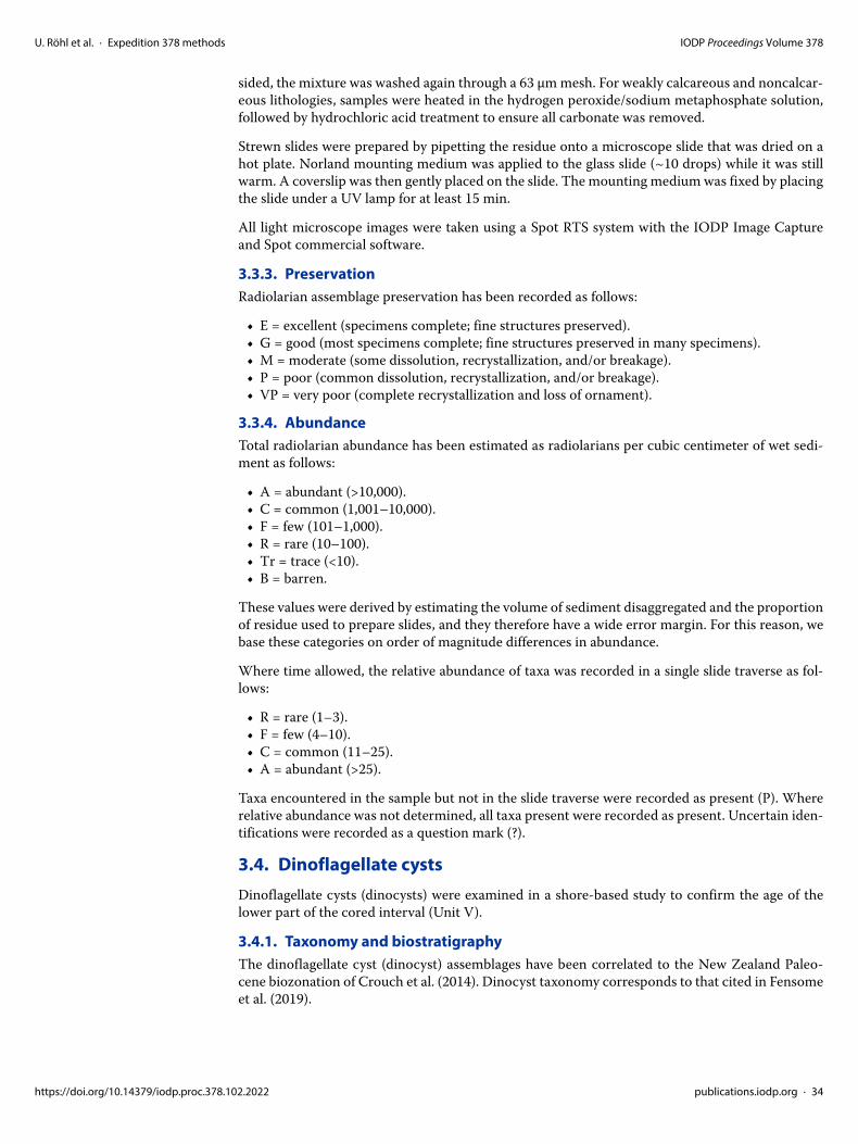
U. Röhl et al. · Expedition 378 methods IODP Proceedings Volume 378
https://doi.org/10.14379/iodp.proc.37
sided, the mixture was washed again through a 63 μm mesh. For weakly calcareous and noncalcar-eous lithologies, samples were heated in the hydrogen peroxide/sodium metaphosphate solution, followed by hydrochloric acid treatment to ensure all carbonate was removed.
Strewn slides were prepared by pipetting the residue onto a microscope slide that was dried on a hot plate. Norland mounting medium was applied to the glass slide (~10 drops) while it was still warm. A coverslip was then gently placed on the slide. The mounting medium was fixed by placing the slide under a UV lamp for at least 15 min.
All light microscope images were taken using a Spot RTS system with the IODP Image Capture and Spot commercial software.
3.3.3. PreservationRadiolarian assemblage preservation has been recorded as follows:
• E = excellent (specimens complete; fine structures preserved).• G = good (most specimens complete; fine structures preserved in many specimens).• M = moderate (some dissolution, recrystallization, and/or breakage).• P = poor (common dissolution, recrystallization, and/or breakage).• VP = very poor (complete recrystallization and loss of ornament).
3.3.4. AbundanceTotal radiolarian abundance has been estimated as radiolarians per cubic centimeter of wet sedi-ment as follows:
• A = abundant (>10,000).• C = common (1,001–10,000).• F = few (101–1,000).• R = rare (10–100).• Tr = trace (<10).• B = barren.
These values were derived by estimating the volume of sediment disaggregated and the proportion of residue used to prepare slides, and they therefore have a wide error margin. For this reason, we base these categories on order of magnitude differences in abundance.
Where time allowed, the relative abundance of taxa was recorded in a single slide traverse as fol-lows:
• R = rare (1–3).• F = few (4–10).• C = common (11–25).• A = abundant (>25).
Taxa encountered in the sample but not in the slide traverse were recorded as present (P). Where relative abundance was not determined, all taxa present were recorded as present. Uncertain iden-tifications were recorded as a question mark (?).
3.4. Dinoflagellate cystsDinoflagellate cysts (dinocysts) were examined in a shore-based study to confirm the age of the lower part of the cored interval (Unit V).
3.4.1. Taxonomy and biostratigraphyThe dinoflagellate cyst (dinocyst) assemblages have been correlated to the New Zealand Paleo-cene biozonation of Crouch et al. (2014). Dinocyst taxonomy corresponds to that cited in Fensome et al. (2019).
8.102.2022 publications.iodp.org · 34

U. Röhl et al. · Expedition 378 methods IODP Proceedings Volume 378
https://doi.org/10.14379/iodp.proc.378
3.4.2. Sample preparationThirteen core catcher samples from Hole U1553D, 8R-CC to 20R-CC, were processed using stan-dard palynological techniques. Around 10 cm3 of sediment was crushed and dried, and the car-bonate and siliceous components were removed by adding 10% HCl and 50% HF, respectively. Heavy liquid separation (using sodium polytungstate) was completed on selected samples, and all samples were then placed in an ultrasonic bath for 30 s prior to sieving. Samples were sieved over a 6 μm mesh, and well-mixed representative fractions of the >6 μm residue were mounted on glass slides using a glycerine jelly medium.
3.4.3. Sample examinationFor each sample, approximately 200 dinocysts were counted and at least one entire slide was scanned for the presence of additional rare taxa. While slides were scanned, spore and pollen taxa were also noted but counts were not completed. Quantitative data are calculated as a percentage of the total dinocyst count and are discussed using the following terms: rare (1%–5%), common (6%–10%), frequent (11%–20%), abundant (21%–40%), and superabundant (>40%).
4. PaleomagnetismShipboard paleomagnetic studies were conducted on both the archive-half and working-half sec-tions from Expedition 378 cores. The primary objectives were to determine the directions of nat-ural remanent magnetization (NRM) components, including the magnetic polarity, and downhole variation of magnetic properties. Routine measurements were carried out on archive-half sections with stepwise alternating field (AF) demagnetization. For discrete samples taken from selected working-half sections, stepwise AF and thermal demagnetization were applied. These data were used for core orientation and magnetostratigraphy construction.
Ocean drilling cores generally carry secondary remanence components or overprints, such as nat-ural viscous remanent magnetization and a steep downward-pointing component imparted by the drilling process. Nonmagnetic core barrels were thus adopted for all cores except those recovered with the XCB coring system. To separate these overprints from the characteristic remanent mag-netization (ChRM), stepwise AF demagnetization in low fields (≤12 mT) was performed. In addi-tion, the downhole orientation tool (Icefield MI-5 core orientation tool) was deployed for all full-length APC cores in Holes U1553A and U1553B to correct the measured core declinations back to true coordinates. All measurement data were uploaded to the LIMS database. The stepwise demagnetization data of the discrete samples were analyzed using principal component analysis to define the ChRM (Kirschvink, 1980). Data visualization (Zijderveld demagnetization plots [Zij-derveld, 1967] and equal-area projections) and principal component analysis were mainly con-ducted using the PuffinPlot desktop application (version 1.03) (Lurcock and Wilson, 2012) and PmagPy software (Tauxe et al., 2016).
4.1. Magnetic measurements on archive-half sectionsThe remanent magnetization of archive-half sections was measured using a pass-through, liquid-helium–free superconducting rock magnetometer (SRM; 2G Enterprises model 760-4k) equipped with direct-current superconducting quantum interference devices (SQUIDs) and an in-line, auto-mated AF demagnetizer capable of reaching a peak field of 80 mT. The measurement of archive halves was conducted using the SRM software (IMS-SRM version 10.3), and an assumed sample area of 17.5 cm2 was adopted for conversion to volume-normalized magnetization units (A/m).
The interval between NRM measurement points was typically 2.5–5 cm at a speed of 10 cm/s. The time to measure each point as well as the AF demagnetization process usually requires 3.5–4 min at 5 cm spacing. The response functions of the pickup coils of the SQUID sensors have a full width of 7.25–8.8 cm at half height. Therefore, data collected within ~4 cm of piece boundaries (or voids) are significantly affected by edge effects. Consequently, all data points within 4.5 cm of sec-tion boundaries (as documented in the curatorial record) were filtered out prior to further pro-cessing. It should be noted that edge effects may also occur in a contiguous core piece if substantial heterogeneity (in intensity or direction) is present. It is more difficult to filter out such artifacts,
.102.2022 publications.iodp.org · 35

U. Röhl et al. · Expedition 378 methods IODP Proceedings Volume 378
but calculating the average direction (using Fisher statistics) for each core piece could provide a means of identifying these problems (Expedition 330 Scientists, 2012). In addition, core distur-bance, often found in the top part of the first section of each core, leads to a surge in magnetization and scattered demagnetization data. Therefore, caution is needed when interpreting those data.
Successive AF demagnetization was performed using the SRM in-line AF demagnetizer on all split archive halves. The in-line AF demagnetizer applies a field to the x-, y-, and z-axes of the SRM in this fixed order (Figure F8A, F8D). Demagnetization fields no higher than 15 mT were used to demagnetize the sections. For most of the cores, three steps were performed after NRM from 3 to 9 mT. No higher AF steps were employed here because (1) the cored materials were mostly weak in NRMs, (2) the shipboard paleomagnetic laboratory is not in a magnetically shielded room and is easily affected by surrounding environments, and (3) previous reports suggested that higher AF demagnetization fields have produced significant anhysteretic remanent magnetization along the z-axis of the SRM (e.g., Harris et al., 2013). AF demagnetization results were plotted individually as vector plots (Zijderveld, 1967) as well as downhole variations with depth. The plots were visually inspected to determine whether the remanence after demagnetization at the highest AF step reflects the ChRM and geomagnetic polarity sequence.
Low-field MS (κ) measured on whole-round core sections using the WRMSL and on archive halves using the SHMSL (see Physical properties) was used to indicate the concentration of mag-netic minerals. Data were compared to discrete cube measurements made with the Agico KLY 4S Kappabridge MS meter. Whole-round records of MS were compared to visual features in the split cores to flag any artifacts or split disturbance.
4.2. Magnetic measurements on discrete samplesOriented discrete samples were collected from working-half sections, nominally 2–3 discrete sam-ples per core. Discrete sample locations were chosen preferentially in fine-grained intervals where drilling deformation was minimal or not visible. In soft sediment, discrete samples were taken with plastic “Japanese” Natsuhara-Giken sampling cubes (7 cm3 sample volume) (Figure F8B). Cubes were manually pushed into the working half of the core, and the “up” arrow on the cube pointed upsection in the core. In lithified sediments and hard rocks, 2 cm cubes (8 cm3 sample volume) were cut with a parallel saw.
Figure F8. A. IODP coordinates for paleomagnetic samples (after Richter et al., 2007). B. Natsuhara-Giken sampling cubes (7 cm3 volume) with sample coordinate system; hatched red arrow is parallel to the up arrow on the sample cube and points in the Z-direction. C. Measurement positions in the JR-6A spinner magnetometer. D. Coordinate system used for the superconducting rock magnetometer on board JOIDES Resolution.
Working half
Double lineat bottom +z
+y
+x Top
Top
Bottom
+x+z
+y
270
000
090
180
090270
North
East
South
West
Archive half
Single lineat bottom
o
o
o
o o
o
+z
+x
+y
BA
Bottom
Upcore
Upcore
+z
+y+x
Magnetometer coordinate system
+z
+y
+x
+x +z
+y+z
+y
+x
Top Archive-halfcoordinate system
Working-halfcoordinate system
D
Up arrow
C
Up arrow
https://doi.org/10.14379/iodp.proc.378.102.2022 publications.iodp.org · 36
U. Röhl et al. · Expedition 378 methods IODP Proceedings Volume 378
https://doi.org/10.14379/iodp.proc.378.1
Incremental AF demagnetization was performed with the DTech AF demagnetizer (model D-2000) for the JR-6A spinner magnetometer with up to 9 mT AF demagnetization for most of the samples because higher AF treatments often record a surge in magnetization with demagnetiza-tion path trending away from the origin, probably suggesting acquisitions of gyroremanent mag-netization (e.g., Snowball, 1997). Several high-coercivity samples underwent higher AF steps up to 50 mT, where the surge of magnetization often occurs at around 20 to 40 mT. Progressive thermal demagnetization was also applied using a thermal specimen demagnetizer (ASC Scientific model TD-48 SC) in 25°C steps up to 175°C. However, thermal treatments appeared to affect the mag-netic minerals in some of the sediments, suggested by an obvious color change to much lighter gray. An increase in magnetization was often observed at ~150°C accompanied by an off-origin trend of the demagnetization path.
Anisotropy of magnetic susceptibility (AMS) was measured on an Agico KLY 4S Kappabridge instrument using the AMSSpin LabVIEW program designed by Gee et al. (2008) and adopted for the shipboard KLY 4S. The KLY 4S Kappabridge measures AMS by rotating the sample along three axes, stacking the data, and calculating the best-fit second-order tensor. It also measures the volume-normalized, calibrated bulk susceptibility (χ).
It is worth mentioning that the SRM is not recommended to measure discrete samples because the resultant demagnetization behavior of the discrete samples becomes very noisy at higher AF treat-ments and difficult for useful magnetic interpretation. Shipboard tests of the reliability of discrete measurements on the 2G SRM showed significant scatter in NRM directions from a standard sam-ple that was measured over hundreds of times. In addition, to avoid contamination by the ambient magnetic field during shipboard measurements, discrete samples were stored in two available cylindrical mu-metal shields (aligned approximately perpendicular to the ambient magnetic field) with low field environments.
4.3. CoordinatesAll magnetic data are reported relative to the IODP orientation conventions: +x points into the face of the working half, +y points toward the left side of the face of the working half, and +z points downsection (Figure F8). The relationship of the SRM coordinates (X-, Y-, and Z-axes) to the data coordinates (x-, y-, and z-directions) is as follows: for archive halves, x-direction = X-axis, y-direc-tion = −Y-axis, and z-direction = Z-axis; for working halves, x-direction = −X-axis, y-direction = Y-axis, and z-direction = Z-axis (Figure F8). The coordinate systems for the spinner magnetome-ter (AGICO model JR-6A) and Natsuhara-Giken sampling cubes are also shown in Figure F8.
4.4. Core orientationPaleomagnetic study of marine sediment cores is greatly enhanced if the angle between magnetic north and the double line orientation marked on the core liner is established through orientation. Core orientation using the APC system employs a nonmagnetic barrel and the Icefield MI-5 core orientation tool mounted on the core barrel. The Icefield MI-5 tool consists of triaxial magnetom-eters and accelerometers. The information from the magnetometers and sensors allows measuring the azimuth and dip of the hole as well as the azimuth of the core. This azimuth, combined with the local magnetic declinations, allows us to reorient the measured core declinations back to true geographic coordinates. In the orientation deployment, the tool is connected to the core barrel in such a way that the double lines on the core liner are at a fixed and known angle relative to its sensors. This angle has been assumed to be zero. Previous expeditions have reported that in gen-eral, these orientation tools have an accuracy of 20°–30°. However, the corrected declinations of the APC cores in the first two holes (U1553A and U1553B) did not turn out to be useful to the interpretation of the paleomagnetic data. This is probably because of the low abundance of ferro-magnetic minerals. Thus, the tool was not deployed in Hole U1553E.
4.5. Magnetostratigraphy constructionThe magnetostratigraphy was constructed by correlating observed polarity patterns with the ref-erence geomagnetic polarity timescale (GPTS) constrained by biostratigraphic units. The chosen GPTS for Expedition 378 is the synthesis of astronomical tuning of Cenozoic through the latest
02.2022 publications.iodp.org · 37

U. Röhl et al. · Expedition 378 methods IODP Proceedings Volume 378
https://doi.org/10.14379/iodp.proc.378
Cretaceous polarity zones compiled for the GTS2012. The Cenozoic portion of this GPTS together with microfossil biozones is shown in Figure F7.
A magnetic reversal was defined when a ~180° shift in the declinations as well as significant shal-lowing of the inclinations were observed in the paleomagnetic data obtained from the pass-through measurements on long, coherent core sections at the 6 mT demagnetization step. This was subsequently verified by the ChRM directions of the discrete samples from the corresponding meter level of the working half. However, polarity reversals occasionally occurring at core section tops were often subject to drilling disturbance and thus were interpreted conservatively.
The naming convention of the polarity patterns follows that of correlative chron and anomaly numbers (e.g., Tauxe et al., 1984; Harland et al., 1990; Cande and Kent, 1992). Normal polarity subchrons are referred to by adding suffixes (n1, n2, etc.) that increase with age. For the younger ages of the timescale (Pliocene–Pleistocene), traditional names are used to refer to the various chrons and subchrons (e.g., Brunhes, Jaramillo, Olduvai).
5. GeochemistryThe shipboard geochemistry program for Expedition 378 conducted a rigorous sampling and ana-lytical program to characterize IW and sediment chemical composition and to constrain the diverse diagenetic and authigenic reactions occurring at Site U1553. Headspace samples were ana-lyzed immediately for routine hydrocarbon monitoring as required for safety and pollution pre-vention protocol. The geochemistry sampling and analysis plan accounted for one to two geochemists on each 12 h shift.
5.1. Hydrocarbon gas sampling and analysesOne headspace gas sample was collected from each Hole U1553A core, usually from the top of the section adjacent to the deepest IW whole-round sample. Headspace gas samples were also taken from cores from additional holes where depths exceeded those of previously drilled holes or where hydrocarbon concentrations required detailed monitoring. Between 3 and 5 cm3 of sediment was sampled immediately after cores were split into sections on the catwalk using a cork borer in soft sediments (Cores 1H–24X) and a metal spatula for more lithified material (below Core 24X and for all other samples). Samples were subsequently extruded into a glass serum vial, sealed with a septum and metal crimp cap, and lightly swirled. After heating the samples at 70°C for 30 min, approximately 5 cm3 of the evolved gas was sampled from the headspace in the vial with a glass syringe and injected into an Agilent 7890 gas chromatograph (GC) equipped with a flame ioniza-tion detector (FID) for rapid estimation of methane (C1), ethane (C2), ethene (C2=), propane (C3), and propene (C3=). Helium was used as the carrier gas. The initial GC oven temperature was 35°C. It was held for 4 min before ramping at 25°C/min to 200°C before a final holding time of 5 min. Data were collected and evaluated with an Agilent Chemstation data-handling program. The chromatographic response was calibrated to three different gas standards containing known vari-able concentrations of low molecular weight hydrocarbons. Check standards were measured reg-ularly.
5.2. Bulk sediment geochemistryIn 1–2 sections per core, approximately 5 cm3 of sediment was sampled adjacent to MAD and XRD sampling for analyses of carbonate and organic matter content and maturity. Additional sam-ples were taken when interesting lithologic changes were observed. Samples were freeze-dried for 12 h and homogenized using an agate mortar and pestle or a shatter box for lithified material. Samples were stored in glass vials until preparation for chemical analyses.
5.2.1. Calcium carbonate analysesCalcium carbonate (CaCO3) content was determined using a CM5015 coulometer. About 10 mg of dry sediment was placed into a glass vial, heated in the acidification module (CM5030), and reacted with 5–10 mL of 1 M HCl. The evolved CO2 was back-titrated to a colorimetric end point.
.102.2022 publications.iodp.org · 38

U. Röhl et al. · Expedition 378 methods IODP Proceedings Volume 378
https://doi.org/10.14379/iodp.proc.378.
Carbonate content, reported as weight percent, was calculated from the inorganic carbon (IC) content based on the assumption that all IC exists as CaCO3:
wt% CaCO3 = wt% IC × 8.33.
Analytical reproducibility was determined by replicate measurements of selected samples. A veri-fication external standard (i.e., 100 wt% CaCO3) was run every 10 samples. Analyses would only continue if values were between 99 and 100 wt%. The coulometer cell was replaced after 24 h or 50 measurements.
5.2.2. Total carbon, nitrogen, and sulfurTotal carbon (TC), nitrogen (N), and sulfur (S) content was determined using a Thermo Electron Flash EA 1112 elemental analyzer equipped with a Thermo Electron packed GC column carbon-hydrogen-nitrogen-sulfur (CHNS)/NCS (polytetrafluoroethylene; length = 2 m; diameter = 6 mm × 5 mm) and thermal conductivity detector (TCD). Aliquots of 12–15 mg of freeze-dried ground sediment were weighed into tin cups. Less than ~4 mg of vanadium oxide was added to each sam-ple to act as a catalyst for total sulfur analyses. Capsules were wrapped and combusted at 950°C in the reactor oven of the instrument with a pulse of O2. Nitrogen oxides were reduced to N2, and the mixture of gases produced (N2, CO2, H2O, and SO2) was separated using the GC and measured using the TCD. The GC oven temperature was held at 65°C between runs. All elemental analyzer measurements were calibrated by comparison to a soil reference material (TC = 3.496 wt%; total nitrogen = 0.365 wt%; total sulfur = 0.063 wt%). Analytical reproducibility was determined by 10 replicate measurements of this standard. Associated standard deviation was 0.02, 0.10, and 0.00 for N, C, and S, respectively. The coefficient of variation was 6.3%, 2.0%, and 2.2% for N, C, and S, respectively. External verification standards (i.e., soil reference material) were run every 10 sam-ples as quality control. Total organic carbon (TOC) was determined as the difference between TC and IC measured by coulometry:
wt% TOC = wt% TC − wt% IC.
Reliable determination of C/N ratios was hampered by the overall low N values. Peak tailing and anomalous values were monitored for combustion column degradation and guided regular clean-ing and replacement.
5.2.3. PyrolysisPyrolysis analysis was conducted on 19 bulk sediment samples from Cores 378-U1553C-42R through 44R and 378-U1553D-19R through 20R to investigate the thermal maturation of the organic matter, hydrocarbon sources, and petroleum potential. Approximately 80 mg of freeze-dried, homogenized sediment was weighed into metal crucibles and measured with a Weatherford Instruments source rock analyzer (SRA) equipped with an infrared section and a FID. Weather-ford Laboratories SRA Rock Standard 533 was used as the calibration and quality control stan-dard. Each sample was heated at 340°C for 3 min, and the volatile hydrocarbons present in the sample were released and measured as S1 peak (mg HC/g rock). After the temperature was increased to 640°C at 25°C/min, the hydrocarbons produced during thermal cracking of kerogen were measured as the S2 peak (mg HC/g rock). The temperature at which maximum release of hydrocarbons occurs during S2 analysis is reported as Tmax. Each sample was then heated from 340° to 390°C, and the released CO2 (mg C/g rock) was measured as the S3 peak. Additional CO2produced by oxidizing the pyrolysis residue at 580°C is the S4 peak. S4 is used along with S1 and S2 to estimate TOC (wt%). Other indirect measurements are the carbon-normalized hydrogen index (HI) (mg HC/g C), the oxygen index (OI) (mg CO2/g C), and the production index (PI):
HI = (100 × S2)/TOC,
OI = (100 × S3)/TOC, and
PI = S1/(S1 + S2).
No hydrocarbon potential (S2) was detected in 11 samples, leading to randomized Tmax values and providing unreliable and overestimated values for other indexes.
102.2022 publications.iodp.org · 39

U. Röhl et al. · Expedition 378 methods IODP Proceedings Volume 378
https://doi.org/10.14379/iodp.proc.378
5.2.4. Major and trace element concentrationsSediment samples for inductively coupled plasma–atomic emission spectrometry (ICP-AES) anal-yses were prepared using a flux fusion approach. (Data produced on the Agilent 5110 inductively coupled plasma–optical emissions spectrometer [ICP-OES] was collected in AES mode and is referred to as “ICP-AES” in the LIMS database. In this document, “ICP-AES” is used to refer to this data.) This technique ensures complete dissolution of the sample material, allowing a full ele-mental analysis. To begin, 100 mg ±1 mg of each sample or a standard (BCR-2, BIR-1, BHVO-2, DNC-1, NBS-1c, PACS-3, W-2, SCo-1, or AGV-1) was weighed on a Cahn C31 microbalance. The 100 mg ±1 mg of sample or standard powder was mixed with 400 mg of lithium metaborate that was preweighed on land and stored in a glass vial covered with Parafilm M. A LiBr solution (10 μL of 0.172 mM) was added to the flux and sediment powder mixture prior to sample fusion to pre-vent the fused bead from sticking to the crucible during cooling. Samples were fused individually in Pt-Au (95:5) crucibles for 2 min at 700°C, 5 min at 1050°C, and 5 min in agitation at 1050°C (12 min total) in an internally rotating induction furnace (Bead and Fuse Sampler TK-4100). The fused beads were transferred into 125 mL high-density polypropylene bottles and dissolved in a 50 mL solution containing 10% trace metal grade HNO3. Each solution bottle was shaken in a Burrell wrist-action shaker until the bead dissolved. Increments of 20 mL of the solution were passed through a 0.45 μm filter into a clean 60 mL wide-mouth high-density polypropylene bottle. From this filtered solution, 0.5 mL was pipetted into a sample tube and diluted with 4.5 mL of 10% HNO3, 10 ppm Y. Within any analytical run, the dilution factor was kept constant for all samples, blanks, and standards, and the ICP-AES approach is similar to the one for IW samples (see Rhi-zons). The standard reference material BHVO-2 was run as an unknown between every five sam-ples. The precision of the BHVO-2 concentrations run as unknowns (n = 17) was <1% for Al2O3, CaO, Fe2O3, MgO, MnO, SiO2, Sr, and TiO2 and <2% for Ba, Cr, K2O, Na2O, Sc, V, Y, and Zr. The precision for La was 12%, for P2O5 was 6%, and for Zn was 13.6%. The measured values of BHVO-2 run as unknowns were accurate within precision.
5.2.5. Repository core analysis for shipboard data (XRF core scanning)XRF elemental records were generated for all core sections with a third-generation Avaatech XRF core scanner and a fourth-generation Avaatech XRF core scanner at the GCR in College Station, Texas. The data presented are available as a shipboard data set in LIMS.
For all the scanned sections of Site U1553, XRF core scanner data were collected every 2 cm down-core over a 1.2 cm2 area with a downcore slit size of 10 mm using generator settings of 10, 30, and 50 kV, a 0.12 mA current for the 10 kV setting, 1.25 mA for the 30 kV setting, a 0.75 mA current for the 50 kV setting, and a sampling time of 6 s directly at the split core surface of the archive half. The 30 kV run was measured using a Pd thick filter, and the 50 kV run was measured using a Cu filter (to lower the background noise).
The split core surface was covered with a 4 μm thin SPEXCerti Prep Ultralene foil to avoid con-tamination of the XRF measurement unit and desiccation of the sediment. Both of the Avaatech XRF core scanners have similar components and thus provide very similar data. Data were acquired using Brightspec silicon drift detectors (Model SiriusSD-D65133BE-INF with 133 eV X-ray resolution), the TopazX high-resolution digital multichannel analyzer, and water-cooled, 100 W rhodium side-window X-ray tubes. Raw data spectra were processed by the analysis of X-ray spectra using the Iterative Least square software (WIN AXIL) package from Canberra Eurisys.
5.3. Interstitial water
5.3.1. Interstitial water sample collection and preservationDuring Expedition 378, a “mudline” sample was collected from within the core liner above the uppermost sediment recovered from the first hole (U1553A), and one sample was collected from between the core liner and sediment at Section 378-U1553B-26X-5, 214.13 mbsf. IW was extracted from sediment cores using two different techniques: squeezing of whole-round intervals and removal using Rhizon samplers. Both techniques were employed to mitigate the disadvan-tages of each (e.g., Dickens et al., 2007; Schrum et al., 2012; Miller et al., 2014). All whole-round and Rhizon samples were taken at room temperature (and pressure) and subsequently stored in
.102.2022 publications.iodp.org · 40

U. Röhl et al. · Expedition 378 methods IODP Proceedings Volume 378
https://doi.org/10.14379/iodp.proc.378
the refrigerator, and we are aware of potential temperature effects on IW chemistry (Sayles and Manheim, 1975; Gieskes, 1975).
5.3.1.1. Whole roundsWhole-round samples for IW were taken on the catwalk after a core was cut into 1.5 m (nominal) sections. The samples subsequently were trimmed to remove potentially contaminated sediment and water. When there was a backlog, some whole rounds were stored in a cold room in a Ziploc bag flushed with nitrogen gas. Squeezing of samples was completed less than 4.5 h after the core arrived on deck.
Extraction of IW was achieved with a Carver laboratory hydraulic press, which extruded IW through a prewashed (with 18.2 MΩ water) Whatman Number 1 filter fitted above a titanium screen within the squeezer and a 0.45 μm polysulfone disposable filter (Whatman Puradisc PES) and then into a precleaned (10% HCl) 60 mL syringe. After squeezing, the compressed cylinder of sediment (squeeze cake) was removed and the squeezing apparatus was cleaned. The compressed sediment squeeze cake was divided and preserved for additional individual postcruise research.
5.3.1.2. RhizonsRhizons are thin tubes of hydrophilic porous polymer. When inserted into a sediment core through a hole in the liner and attached to a collection tube and an evacuated syringe, they permit collection of small volumes (typically <12 mL) of IW through suction filtering. Such IW samples come without removal of whole rounds, thus preserving the sedimentary record. They also enable water sampling at very high depth resolution (<5 cm). For Expedition 378, the chosen samplers were Rhizon CCS 5 cm (flat tip and 2.5 mm outer diameter) from Rhizosphere Research Products (Netherlands), which were prerinsed three times with 18.2 MΩ deionized water.
Rhizon sampling commenced after core sections were run through the Special Task Multisensor Logger (STMSL) and during the time (nominally 3–4 h) when cores equilibrate for NGR measure-ment (see Physical properties). The extraction of IW from each Rhizon was ended when the syringe was full or after ~2 h, whichever came first, so that Rhizon sampling was kept at the pace of the core recovery and equilibration and did not interrupt core flow.
A sample of fluid from between the core liner and the sediment was collected at the top of Section 378-U1553B-26X-5 and filtered through a Rhizon in the laboratory to determine whether seawa-ter in the edge of the liner (a result of smaller diameter XCB recovery) was biasing or contaminat-ing IW results from XCB cores. Our shipboard measurements suggest seawater was not affecting the major features of chemical profiles in the pore fluids and sediments, and further onshore anal-yses will test for potential outliers in the data. There was a delay between Rhizon sample collection and subsequent transfer to individual vials for storage and/or analyses of 10 to ~15 h, and samples from Cores 378-U1553B-11H through 14H were left for last. Most samples were kept in either the refrigerator or the cold room in their individual syringes that were capped and stored in Ziploc bags. Therefore, we do not expect any major alteration to their chemical composition.
5.3.2. Interstitial water analytical methods
5.3.2.1. SalinitySalinity was analyzed with a Fisher Model S66366 portable salinity refractometer. A few drops of sample were applied to the daylight plate assembly with a pipette, and the measurement was read through the eyepiece, with typical measurement precision of ±1‰. Blanks (18.2 MΩ deionized water) and International Association for the Physical Sciences of the Oceans (IAPSO) water (OSIL Environmental Instruments and Systems, Batch P162) were analyzed routinely to check for con-tamination. Salinity measurements were completed days after collection of the IW. Therefore, for smaller size aliquot samples (<1 mL), artificially high values are likely.
5.3.2.2. Alkalinity and pHpH and alkalinity were measured within 24 h after squeezing to avoid degradation (Gieskes, 1975). The pH was measured using a combination glass electrode (Brinkman pH electrode), and alkalin-ity was determined by Gran titration using an autotitrator (Metrohm 794 Titrino). A total of 3 mL of IW was titrated with 0.1 M HCl at 25°C. The electrode was calibrated using a series of buffers
.102.2022 publications.iodp.org · 41

U. Röhl et al. · Expedition 378 methods IODP Proceedings Volume 378
https://doi.org/10.14379/iodp.proc.378.1
with a pH of 4, 7, and 10. IAPSO seawater was analyzed every ~12 h or after a period of no use to check accuracy. Alkalinity was typically within 2% of the expected value for IAPSO (2.325 mM).
5.3.2.3. Ion chromatographyConcentrations of major anions (Cl−, SO4
2−, and Br−) and major cations (Ca2+, Na+, Mg2+, and K+) were measured on a Metrohm 850 professional ion chromatograph with an 858 professional sam-ple processor. IW was diluted 1:100 with 18.2 MΩ deionized water in preparation for ion chroma-tography analysis. Diluted IAPSO seawater was analyzed every 10 samples as a consistency standard and to create a six-point calibration curve. Precision was 5% for Ca2+ and Br− and 3% for the other ions.
5.3.2.4. Inductively coupled plasma–atomic emission spectroscopySuites of major (S, Ca, Mg, K, and Na) and minor (B, Ba, Fe, Li, Mn, P, Si, and Sr) elements were analyzed with an Agilent Technologies 5110 spectrometer ICP-AES. The shipboard ICP-AES pro-cedure is similar to that of Murray et al. (2000). Samples and standards were diluted using 2% ultrapure HNO3 spiked with 10 ppm Y with dilution ratios of 1:10. Samples were typically run in batches of 35–85 samples. With every batch run for major elements (S, Ca, Mg, K, and Na), a seven-point calibration curve was created using different dilution levels of IAPSO seawater. For minor elements (B, Ba, Fe, Li, Mn, P, Si, and Sr), an eight-point calibration curve was created using synthetic seawater spiked with minor elements to varying degrees. This was then used to convert background-corrected intensities to concentrations. Additionally, the calibration curves included four extra standards that were spiked with the trace elements and had IAPSO as a base rather than synthetic seawater to ensure that no matrix effects were imposed by the synthetic seawater. The IAPSO dilutions for the major element calibration curve were also included in the trace element calibration curve for the trace elements with detectable concentrations. All of these standards were analyzed at the beginning of the run to construct a calibration curve using the Agilent soft-ware, and they were also analyzed a second time as unknowns at the end of the run to check accu-racy and drift. An IAPSO standard spiked with trace elements was run every five to seven samples to further monitor drift and precision of each element throughout the run. Three blanks were run with every batch to check for contamination, to allow for blank subtractions, and to calculate the detection limits of each element. Additionally, four samples that span the range of concentrations (selected after the first run) were also analyzed in each subsequent run to check for interrun pre-cision of the samples.
The intrarun precision was calculated as the standard deviation of the spiked IAPSO standards (run as unknowns between every five to seven samples) divided by their average. The first and third run had <1% intrarun precision, and the second run had ~3% intrarun precision for every element except Fe. For Fe concentrations, many of the samples were below the detection limit (0.2 μM), and the triplicate measurements of samples within a few micrometers above had a standard deviation of ±0.2 μM and must therefore be interpreted with caution. Higher concentrations of Fe had a precision of <1%, similar to the other elements. The standards measured as unknowns were accurate within the precision of the known concentrations of the spiked IAPSO standard. The interrun precision was <3%, calculated as the standard deviation of a sample run in each of the three runs divided by the average of the concentrations generated in each of the three runs.
5.3.2.5. SpectrophotometryDissolved ammonium (NH4
+) and phosphate (PO43−) were determined spectrophotometrically
using an Agilent Cary 100 ultraviolet-visible light spectrophotometer according to the method of Solórzano (1969) for ammonium concentrations with a 2% precision (13% for concentrations below 200 μM). Phosphate concentrations were measured according to the method described by Strickland and Parsons (1968) as modified by Presley (1971). The precision was 3 μM for phos-phate concentrations up to 10 μM.
5.4. Microbiology samplingA 5 cm3 syringe sample and a ~2 cm3 syringe sample were obtained for shore-based microbiology DNA analysis and cell counting, respectively. For Cores 378-U1553A-1H through 5H, the pairs of microbiology samples were taken on every other section and adjacent to the whole-round IW
02.2022 publications.iodp.org · 42

U. Röhl et al. · Expedition 378 methods IODP Proceedings Volume 378
https://doi.org/10.14379/iodp.proc.37
sample taken on the catwalk. Samples were collected from the anticipated future working-half sec-tion based on predrawn core splitting lines. For cores deeper than Core 5H, one set of the two microbiology syringe samples was taken every other core until the sediments became too stiff to sample with the syringes.
5.4.1. Sampling for cell countingA set of sterilized 2.5 cm3 syringes with the tapered tips removed was provided to the geochemis-try laboratory before departure. These syringes were used to collect samples for cell counting. After a core was sectioned on the catwalk and a whole-round IW sample was sliced off with an ethanol-sterilized spatula, a syringe was plunged into the working-half section of the exposed core. While the plunger was held, about 2.0 cm3 of sediment was ejected from the syringe into a tube containing 10% filtered formalin solution. The tubes were labeled and stored in a refrigerator at 4°C within 20 min after arrival on the catwalk.
5.4.2. Sampling for DNA/RNA analysisSamples for DNA/RNA were also collected on the catwalk from the cut core section adjacent to the 2.5 cm3 syringe sample for cell counting on the future working-half sections. Sterilized 10 mL syringes with the tapered tips removed were used to extract 5–10 cm3 of sediment. Each syringe that contained sediment was placed in a heat-sealed clear plastic bag. This bag was placed in a clear plastic bag and heat sealed again. Samples were processed and stored in a −80°C freezer within 15 min after arrival on the catwalk.
6. Physical propertiesHigh-resolution physical property measurements were made during Expedition 378 to aid litho-stratigraphic characterization and to contribute to hole-to-hole stratigraphic correlation, detec-tion of hiatuses, and identification of differences in the composition and texture of sediment. A variety of techniques and methods were used on whole-round sections, section halves, and dis-crete samples to characterize the Site U1553 cores.
6.1. General sampling and measurement sequence
6.1.1. Whole-round core measurementsAll whole-round sections were equilibrated to ambient room temperature (~20°C) and pressure for ~4 h. After equilibration, core sections were run through the WRMSL at a 2.5 cm sampling resolution to generate measurements of density by gamma ray attenuation (GRA), MS, and com-pressional P-wave velocity (on the P-wave logger [PWL]). P-wave velocity was not measured on XCB cores from Holes U1553A, U1553B, or U1553E or on any cores from Holes U1553C or U1553D because of insufficient contact of the sediments with the core liner. All core sections were measured with the spectral NGRL. In addition to the standard suite of physical properties mea-surements, all whole-round core sections were imaged using the X-Ray Imager (XRI) prior to split-ting.
Core sections from Holes U1553B–U1553E were run through the STMSL to measure GRA bulk density and MS at a lower sampling resolution (5 cm) prior to equilibration to help with rapid stratigraphic correlation to inform drilling decisions. Three cores from Hole U1553C (31R–33R) were run through the STMSL in an attempt to identify a potentially critical stratigraphic interval. All of these fast-tracked sections were remeasured using the WRMSL at a 2.5 cm sampling resolu-tion following the standard 4 h thermal equilibration period because some of the physical proper-ties measurements are particularly sensitive to temperature. Each core section was then run through the NGRL at a 10 cm resolution.
Thermal conductivity was measured on one whole-round section per sediment core (typically Section 3). Thermal conductivity measurements were taken by inserting a needle probe into a small hole drilled through the plastic core liner close to the middle of the core section. They were taken only on cores soft enough to insert and maintain sufficient contact with the needle probe.
8.102.2022 publications.iodp.org · 43

U. Röhl et al. · Expedition 378 methods IODP Proceedings Volume 378
After splitting, the archive half of each section was passed through the SHMSL for measurement of MSP and color reflectance. Compressional P-wave velocity measurements were made on the x-axis of the working halves (usually two sections per core). Additional P-wave measurements were made during intervals where there was a clear lithostratigraphic change. Z-axis P-wave measure-ments were attempted on the first three cores of Hole U1553A using the P-wave bayonet system inserted into the working half. Because of insufficient contact between the sediment and the sen-sors, these measurements were highly inaccurate. Because z-axis P-wave measurements are destructive to the working halves and there was poor data quality, it was decided to forgo the mea-surement on the remaining cores.
Discrete MAD samples were collected from the working halves to calculate wet bulk density, dry bulk density, water content, porosity, and grain density. Generally, two MAD samples were taken per core from Sections 2 and 5 or in the same sections where the discrete P-wave measurements were taken, and samples were carefully selected to cover the representative lithology of each core. Care also was taken to avoid locations of obvious drilling disturbance and regions of significant strati-graphic interest. These ~10 cm3 samples were measured for wet mass, dry mass, and dry volume, and using these measurements, porosity, salt volume, bulk density, and grain density were calculated. A summary of the physical properties sampling strategy for Expedition 378 is shown in Table T8.
6.1.2. Downhole temperature measurementsDuring APC coring operations in Hole U1553A, formation temperature measurements were taken in three cores (4H, 7H, and 10H) using the APCT-3 tool, which replaces the normal coring shoe. One in situ temperature measurement was also taken using the Sediment Temperature 2 (SET2) tool in the Hole U1553D drilled interval (during drill down) at 181 mbsf.
6.2. Whole-Round Multisensor Logger measurementsGRA bulk density, P-wave velocity, and MS were measured nondestructively using the WRMSL (Figure F9). To optimize the measurement process, sampling intervals and measurement integra-tion times were the same for all sensors. Sampling intervals were set at 2.5 cm with an integration time of 3 s for each measurement on the WRMSL and at 5 cm with an integration time of ~1 s for each measurement on the STMSL when data were required immediately for stratigraphic correla-tion. These sampling intervals are common denominators of the distances between the sensors installed on the STMSL and WRMSL (30–50 cm), which allows sequential and simultaneous mea-surements. After every core, quality was monitored by passing a single core liner filled with deion-ized water through the STMSL or WRMSL.
6.2.1. Gamma ray attenuation bulk densityBulk density can be used to estimate the pore volume in sediment and evaluate the consolidation state of sediment. GRA bulk density is an estimate of bulk density based on the attenuation of a gamma ray beam. The beam is produced by a 137Cs gamma ray source at a radiation level of 370 MBq within a lead shield with a 5 mm collimator and then directed through the whole-round core
Table T8. Physical properties sampling strategy, Expedition 378. STMSL = Special Task Multisensor Logger, WRMSL = Whole-Round Multisensor Logger, NGR = natural gamma radiation, SHMG = Section Half Measurement Gantry, MAD = moisture and density, SHMSL = Section Half Multisensor Logger. NA = not applicable. Download table in CSV format.
Measurement
Holes U1553A, U1553B, U1553E Holes U1553C and U1553D
Cores Section(s)
Sampling frequency
(cm)
Time/section (min) Cores Sections
Sampling frequency
(cm)
Time/section (min)
STMSL All (U1553B and U1553E only) All 5. 2 All (U1553D only); 31R–33R (U1553C) All 5. 2WRMSL All All 2.5 7 All All 2.5 7NGR All All 10. 12 All All 10. 12ThermCon (TK) All (U1553A and U1553B only) 3 1/core 30 None NA NA 30SHMG (caliper x) All 2, 5 NA 5 All Variable NA 5Shear strength All (U1553A only) 2, 5 NA NA None NA NA NACompressional strength All (U1553A only) 2, 5 NA NA None NA NA NAMAD All 2, 5 NA NA None NA NA NASHMSL All All 2.5 6 All All 2.5 6
https://doi.org/10.14379/iodp.proc.378.102.2022 publications.iodp.org · 44

U. Röhl et al. · Expedition 378 methods IODP Proceedings Volume 378
https://doi.org/10.14379/iodp.proc.378
at a spatial resolution of <1 cm. The gamma ray detector on the opposite side of the core from thesource includes a scintillator and an integral photomultiplier tube to record the gamma radiationthat passes through the core. The attenuation of gamma rays occurs primarily by Compton scat-tering, in which gamma rays are scattered by electrons in the formation; the degree of scattering isrelated to the material bulk density. Therefore, for a known sample thickness, the density (ρ) isproportional to the intensity of the attenuated gamma rays and can be expressed as
ρ = ln(I0/I)/(μd),
where
I = the measured intensity of gamma rays passing through the sample,I0 = gamma ray source intensity,μ = Compton attenuation coefficient, andd = sample diameter.
μ and I0 are treated as constants such that ρ can be calculated from I.
In general, WRMSL measurements are only accurate when taken on a completely filled core linerwith minimal drilling disturbance. Otherwise, measurements tend to underestimate true values.The gamma ray detector is calibrated with sealed calibration cores (one standard core liner filledwith distilled water and aluminum cylinders of various diameters). To establish the calibrationcurves, gamma ray counts were taken through each aluminum cylinder for 60 s. Each aluminumcylinder has a density of 2.7 g/cm3, and the diameter (d) is 1, 2, 3, 4, 5, or 6 cm. The relationshipbetween I and μd is
ln(I) = A(μd)2 + B(μd) + C,
where A, B, and C are coefficients determined from the calibration.
Recalibration was performed as needed when the deionized water QA/QC standard deviated sig-nificantly (more than a few percent) from 1 g/cm3.
There is a systematic offset in GRA bulk density and MAD bulk density in data from HolesU1553C and U1553D, where rotary coring yielded cores of smaller diameter, compared to theGRA and MAD measurements in Holes U1553A, U1553B, and U1553E (piston cored), leading toan underestimation of GRA bulk density by the WRMSL instrument. This systematic underesti-mation can be corrected to compare with the measured MAD values by multiplying by a correc-tion factor of 1.10. This was determined by linear regression (R2 = 0.997; ρ < 0.0001), which wehave applied in analyses that rely on GRA bulk density. Throughout this volume, we have pre-sented the raw (uncorrected) GRA bulk density values in the figures.
Figure F9. Whole-Round Multisensor Logger. The Special Task Multisensor Logger is almost identical and only excludes theP-wave logger. The water standard is measured at the end of each core for QA/QC purposes.
PP-wave logger-wave logger
Gamma ray Gamma ray attenuation attenuation densitometerdensitometer
Water standardWater standard
Magnetic Magnetic susceptibility susceptibility loop sensorloop sensor
.102.2022 publications.iodp.org · 45

U. Röhl et al. · Expedition 378 methods IODP Proceedings Volume 378
https://doi.org/10.14379/iodp.proc.378
6.2.2. Magnetic susceptibilityMS (χ) is a measure of the degree to which a material can be magnetized by an external magnetic field:
χ = M/H,
where M is the magnetization induced in the material by an external field of strength H. MS is primarily sensitive to the concentration of ferromagnetic minerals (e.g., magnetite and maghemite) and thus can commonly be related to mineralogical composition (e.g., terrigenous versus biogenic materials) or the diagenesis of magnetic minerals. Ferromagnetic minerals have a specific MS several orders of magnitude higher than clay, which has paramagnetic properties. Car-bonate layers, opal, water, and plastic (core liner) have small negative MS values. Calcareous and biogenic deposits with very small amounts of clays and iron-bearing mineral debris thus have val-ues approaching the detection limit of MS meters.
Measurements were made using a Bartington MS2C loop sensor with a 9 cm diameter. An oscilla-tor circuit in the sensor operates at a frequency of 0.565 kHz and an AF of ~140 A/m to produce a low-intensity, nonsaturating alternating magnetic field. Sediment or hard rock core sections going through the influence of this field cause a change in oscillator frequency. Frequency information returned in pulse form to the susceptometer is converted into MS. The loop sensor has a spatial resolution of 23–27 mm and is accurate to within 2%.
6.2.3. P-wave velocityP-wave velocity data can be used to evaluate the material’s porosity, cementation, bulk density, and lithology as well as state of stress, temperature, and fabric or degree of fracturing. Compressional P-wave velocity (VP) is defined by the time required for a compressional wave to travel a specific distance:
VP = d/tcore,
where d is the path length of the wave across the core and tcore is the traveltime through the core.
The PWL measures the traveltime of 500 kHz ultrasonic waves horizontally across the core at 2.5 cm intervals while it remains in the core liner. Waves are transmitted to the core by plastic trans-ducer contacts connected to linear actuators. Pressure is applied to the actuators to ensure cou-pling between the transducers and the core liner. P-wave velocity transducers measure total traveltime of the compressional wave between transducers. The wave travels horizontally across the whole-round core and core liner. The total observed traveltime tcore is composed of
• tdelay = time delay related to transducer faces and electronic circuitry,• tpulse = delay related to the peak detection procedure,• tliner = transit time through the core liner, and• tcore = traveltime through the sediment.
The system is calibrated using a core liner filled with distilled water, which provides control for tdelay, tpulse, and tliner. From these calibrations, VP can be calculated for the whole-round specimens in core liners as
VP = (dcl − 2dliner)/(to − tpulse − tdelay − 2tliner),
where
dcl = measured diameter of core and liner,dliner = liner wall thickness, andto = measured total traveltime.
The above equation assumes that the core completely fills the core liner. Therefore, data collection from the WRMSL’s PWL was disabled for most of the cores recovered with the XCB system and all of the cores recovered with the RCB system because they often did not fill the core liner and thus produced poor quality data.
.102.2022 publications.iodp.org · 46
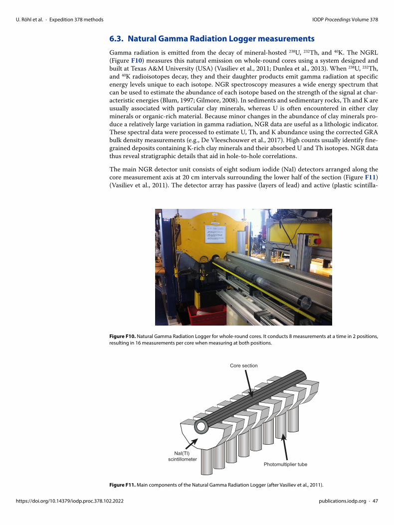
U. Röhl et al. · Expedition 378 methods IODP Proceedings Volume 378
https://doi.org/10.14379/iodp.proc.37
6.3. Natural Gamma Radiation Logger measurementsGamma radiation is emitted from the decay of mineral-hosted 238U, 232Th, and 40K. The NGRL (Figure F10) measures this natural emission on whole-round cores using a system designed and built at Texas A&M University (USA) (Vasiliev et al., 2011; Dunlea et al., 2013). When 238U, 232Th, and 40K radioisotopes decay, they and their daughter products emit gamma radiation at specific energy levels unique to each isotope. NGR spectroscopy measures a wide energy spectrum that can be used to estimate the abundance of each isotope based on the strength of the signal at char-acteristic energies (Blum, 1997; Gilmore, 2008). In sediments and sedimentary rocks, Th and K are usually associated with particular clay minerals, whereas U is often encountered in either clay minerals or organic-rich material. Because minor changes in the abundance of clay minerals pro-duce a relatively large variation in gamma radiation, NGR data are useful as a lithologic indicator. These spectral data were processed to estimate U, Th, and K abundance using the corrected GRA bulk density measurements (e.g., De Vleeschouwer et al., 2017). High counts usually identify fine-grained deposits containing K-rich clay minerals and their absorbed U and Th isotopes. NGR data thus reveal stratigraphic details that aid in hole-to-hole correlations.
The main NGR detector unit consists of eight sodium iodide (NaI) detectors arranged along the core measurement axis at 20 cm intervals surrounding the lower half of the section (Figure F11) (Vasiliev et al., 2011). The detector array has passive (layers of lead) and active (plastic scintilla-
Figure F10. Natural Gamma Radiation Logger for whole-round cores. It conducts 8 measurements at a time in 2 positions, resulting in 16 measurements per core when measuring at both positions.
Figure F11. Main components of the Natural Gamma Radiation Logger (after Vasiliev et al., 2011).
NaI(Tl) scintillometer
Photomultiplier tube
Core section
8.102.2022 publications.iodp.org · 47

U. Röhl et al. · Expedition 378 methods IODP Proceedings Volume 378
https://doi.org/10.14379/iodp.proc.37
tors) shielding to reduce the background environmental and cosmic radiation. The overlying plas-tic scintillators detect incoming high-energy gamma and muon cosmic radiation and cancel this signal from the total counted by the NaI detectors.
Each measurement run consisted of two sample positions 10 cm apart for a total of 16 measure-ments per 150 cm section. The quality of the energy spectrum measured in a core depends on the concentration of radionuclides in the sample but also on the counting time, and higher times yield better spectra. Counting times were chosen as 5 min per position or ~10 min per section, yielding statistically significant energy spectra (Vasiliev et al., 2011).
During Expedition 378, a software error resulted in overwrite of the calibration file. As a result, all core sections measured used an incomplete calibration file, and the NGR calibration files in the LIMS database are missing the slope and intercept for channel to energy conversion. Although missing energy conversion information does not affect data reduction and reported counts/s, threshold channel number picks can affect the data reduction on reported counts/s in the LIMS database. Core sections were run with threshold channel numbers either one higher or the same as would have been picked by hand using a complete calibration, and even though picks of neighbor-ing channels have a statistically insignificant impact on the overall data, concentration studies require a complete set of calibrations. A complete calibration file set is available in NGR_CALI-BRATION in Supplementary material.
6.4. Thermal conductivity measurementsThermal conductivity is an intrinsic material property for which values depend on the chemical composition, porosity, density, structure, and fabric of the material. After NGR measurements were completed, thermal conductivity was measured with the Teka Bolin TK04 system using a needle probe method in full-space configuration for whole-round sediment cores (Von Herzen and Maxwell, 1959). The probes contain a heater wire and calibrated thermistor.
The needle probe was inserted into a 2 mm diameter hole drilled through the liner along one of the lines that later guided core splitting. To avoid interference from air flow in the laboratory, the core was placed into an enclosed box outfitted with foam (Figure F12). The calibrated heat source of the probe was then turned on, and the increase in temperature was recorded over 80 s. A heat-ing power of 2 to 2.5 W/m was typically used. The solution to the heat conduction equation with a line source of heat was then fit to the temperature measurements to obtain the thermal conductiv-ity. Because the probe is much more conductive than sediment, it is assumed to be a perfect con-ductor. Under this assumption, the temperature of the superconductive probe has a linear relationship with the natural logarithm of the time after the initiation of the heat:
T(t) = (q/4πk) × ln(t) + C,
where
Figure F12. Thermal conductivity TK04 (Teka Bolin) system showing the insulated case in which the thermal conductivity measurements were obtained.
8.102.2022 publications.iodp.org · 48

U. Röhl et al. · Expedition 378 methods IODP Proceedings Volume 378
https://doi.org/10.14379/iodp.proc
T = temperature (K),q = heat input per unit length per unit time (J/m/s),k = thermal conductivity (W/[m·K]),t = time after the initiation of the heat (s), andC = instrumental constant.
Three measuring cycles were automatically performed to calculate average conductivity. A self-test, which included a drift study, was conducted at the beginning of each measurement cycle. Once the probe temperature stabilized, the heater circuit was closed and the temperature rise in the probe was recorded. Thermal conductivity was calculated from the rate of temperature rise while the heater current was flowing. Temperatures measured during the first 80 s of the heating cycle were fitted to an approximate solution of a constantly heated line source (Kristiansen, 1982; Blum, 1997). For Site U1553, thermal conductivity profiles of sediment and rock sections were used along with in situ temperature measurements to determine heat flow using methods de-scribed in Pribnow et al. (2000).
Measurement errors were 5%–10%. Thermal conductivity measurements were routinely taken in one section per core (typically Section 3 or 4) for Hole U1553A and Cores 378-U1553B-27X through 29X, which extend past the bottom of Hole U1553A. Thermal conductivity measure-ments were not taken on cores from Holes U1553C and U1553D because cracks in the cores due to rotary coring and lithified sediments caused poor coupling of the needle probe to the sediment. No measurements were taken on cores from Hole U1553E because it spanned the same depths as Holes U1553A and U1553B.
6.5. X-ray imagingX-ray images of all cores were produced to evaluate bioturbation intensity, drilling disturbance, sedimentary structures, and clast abundance. Images were obtained on all whole-round core sec-tions prior to splitting and often during the 4 h thermal equilibrium period because X-ray imaging is not temperature sensitive. The onboard XRI is composed of a Teledyne ICM CP120B X-ray gen-erator and a detector unit. The generator works with a maximum voltage of 120 kV and a tube current of 1 A, and it has a 0.8 mm × 0.5 mm focal spot. The generator produces a directional cone at a beam angle of 50° × 50°. The detector unit is located 65 cm from the source and consists of a Go-Scan 1510 H system composed of an array of complementary metal oxide semiconductor (CMOS) sensors arranged to offer an active area of 102 mm × 153 mm and a resolution of 99 μm. Core sections were run through the imaging area at 12 cm intervals, providing images of 15 cm onto the detector and allowing an overlap of 3 cm.
Tests were conducted on whole-round sections to obtain the best image resolution for determin-ing the internal structure of cores. The XRI settings were then changed to adjust to the varying lithologies of the cores. The number of images stacked was 20, taken at exposure times of 300 s, and the current was kept at 0.7 mA. The voltage ranged between 70 and 90 kV; higher voltages were used for denser lithologies.
The raw images were collected as 16-bit images and were processed with the IODP in-house pro-cessing utility in the Integrated Measurement System software (version 1.3). The software applies corrections for the detector (gain and offset corrections), compensates for core shape and thick-ness, and adjusts the image contrast. The Savitzky-Golay FIR filter was chosen to smooth images. The resulting processed images include a masked background, the depth scale of the section, and the acquisition parameters. The software applies different processing to APC or HLAPC cores than to RCB cores. Some sections where the processing utility did not give good results were reprocessed, first with the LeVay processing software and later with the processing utility (images are available upon request from the IODP Data Librarian: [email protected]).
6.6. Section Half Multisensor Logger measurementsWe measured color reflectance and MS on archive halves using the SHMSL (Figure F13). The archive half was placed on the core track, above which an electronic platform moves along a track recording the height of the split surface with a laser sensor. The laser establishes the location of the
.378.102.2022 publications.iodp.org · 49

U. Röhl et al. · Expedition 378 methods IODP Proceedings Volume 378
https://doi.org/10.14379/iodp.proc.37
bottom of the section, and then the platform reverses the direction of movement, moving from bottom to top making measurements of MSP and color reflectance. During Expedition 378, MSP and color reflectance data were collected at a 2.5 cm resolution. These measurements have a suffi-cient resolution for comparison with the results obtained from the MS loop on the WRMSL.
6.6.1. Color reflectance spectrometryThe color reflectance spectrometer uses an Ocean Optics 30 mm integrating sphere and both a halogen and LED light source, which cover wavelengths from ultraviolet through visible to near infrared. The measurements were taken from 380 to 900 nm wavelengths at 2 nm intervals. The approximately 3 s data acquisition offset was applied for the entire scan of the archive half. The data are reported using the L*a*b* color system, in which L* is lightness, a* is redness (positive) versus greenness (negative), and b* is yellowness (positive) versus blueness (negative). The color reflectance spectrometer calibrates on two spectra, pure white (reference) and pure black (dark). Color calibration was conducted approximately once every 6 h (twice per shift).
6.6.2. Point magnetic susceptibilityMSP was measured at a 2.5 cm resolution using a Bartington MS2 meter and an MS2K contact probe with a flat 15 mm diameter round sensor with a field of influence of 25 mm and an opera-tion frequency of 930 Hz. The instrument averages three measurements from the sensor for each offset, giving an accuracy of ~5%. The spatial resolution of the MSP instrument is ~3.8 mm, higher than that of the whole-round MS. This measurement is therefore better suited for sections con-taining broken pieces <4 cm in length (the spatial resolution of whole-round MS). As with whole-round measurements, the output displayed by the MSP sensor can be converted to dimensionless SI units by multiplying by 10−5. The probe is zeroed in air before each measurement location to avoid influence from the metal track. The MSP meter was calibrated by the manufacturer before
Figure F13. Section Half Multisensor Logger used for high-resolution color reflectance measurements and discrete mag-netic susceptibility measurements along archive halves. Ocean Optics USB4000 spectrophotometer and magnetic suscep-tibility point sensor.
Section Half Multisensor Logger (SHMSL)
Core section
Infrared laser sensor
Magneticsusceptibilitypoint sensor
Colorreflectance
point sensor
Track
8.102.2022 publications.iodp.org · 50

U. Röhl et al. · Expedition 378 methods IODP Proceedings Volume 378
https://doi.org/10.14379/iodp.proc.378
installation on the ship and is quality checked every ~6 h at the same time as color reflectance sensor calibration.
6.7. Section Half Measurement Gantry measurementsP-wave velocity measurements were performed on working halves before samples were taken. P-wave velocity measurements were made using the x-axis caliper contact probe transducers on the Section Half Measurement Gantry (SHMG) (Figure F14) for two analyses per core, generally in Sections 2 and 5. Additional measurements were taken where there was a change in lithology. Measurements were usually taken at ~75 cm in the section and as close as possible to where the MAD sample was taken. However, if this interval provided poor sediment/transducer coupling (e.g., had significant cracking), exhibited drilling disturbance, was in between biscuits of core, or was not representative of the core section, different positions were selected to ensure viable data.
The P-wave velocity system uses Panametrics-NDT Microscan delay line transducers, which transmit at 0.5 MHz. The signal received through the section half or the discrete sample was
Figure F14. A. Section Half Measurement Gantry showing the x-axis caliper and y- and z-axis bayonets used to measure P-wave velocity on working halves of soft-sediment cores or discrete samples of indurated sediment. B. x-axis caliper tool in closed position. C. Different axes in working halves.
Z bayonet
Y bayonet
X caliper
A B
Working half Up
Double line
Split-core face
x
z
y(90°)
C
.102.2022 publications.iodp.org · 51

U. Röhl et al. · Expedition 378 methods IODP Proceedings Volume 378
https://doi.org/10.14379/iodp.proc.37
recorded by the computer attached to the system. The first P-wave arrival was selected by the autopicking software and confirmed by a manual check. The distance between transducers was measured with a built-in linear voltage displacement transformer. Calibration was performed with a series of acrylic cylinders of differing thicknesses and a known P-wave velocity of 2750 ± 20 m/s. The determined system time delay from calibration was subtracted from the picked arrival time to give a traveltime of the P-wave through the sample. The thickness of the sample (calculated by the linear voltage displacement transformer, in meters) was divided by the traveltime (in seconds) to calculate P-wave velocity in meters per second.
6.8. Shear and compressional strength measurementsShear strength is the resistance of a material to failure in shear. Shear stress in unconsolidated materials is resisted only by the network of solid particles. Shear strength (τf) can be expressed as a function of the effective normal stress at failure (σ′), the effective cohesion (c′), and the friction angle (φ′):
τf = c′ + σ′tan(φ′),
where c′ and φ′ are the shear strength parameters that define a linear relationship between τf and φ′, according to the Mohr-Coulomb failure criterion.
Shear strength parameters can be determined by multiple laboratory tests. The c′ and φ′ are rele-vant in situations where field drainage conditions correspond to test conditions. The shear strength of a soil under undrained conditions (IW drainage does not occur during failure) is differ-ent from that under drained conditions (IW drainage occurs).
Undrained shear strength (Su) can be expressed in terms of total stress in the case of fully saturated materials of low permeability (e.g., clays). The most common strength tests in shipboard laborato-ries are the vane shear and penetrometer tests, which provide measurements of undrained shear strength (Blum, 1997).
During Expedition 378, Su was measured in undisturbed soft sediment using a handheld Torvane shear device on working halves because the commonly employed automated vane shear device was broken. Using the Torvane device, undrained shear strength was determined by inserting a vane into the split core and rotating it while maintaining a constant vertical pressure at a constant rate such that failure occurred in 5–10 s. Measurements were made with the vane rotation axis perpendicular to the split surface. The maximum shear value was then read off the Torvane dial in kilograms per square centimeter (kg/cm2). The 1.0 and 2.5 adapters were used, depending on the stiffness of the sediment. The mechanical scale is in units of kilograms per square centimeter, and the data were uploaded to the LIMS database in this form.
A pocket penetrometer was used to measure the unconfined compressive strength of the uncon-solidated sediments. The penetrometer is a flat-footed, spring-operated device used to measure compressive strength by pushing a 0.25 inch (6.4 mm) diameter probe 0.25 inches (6.4 mm) deep (to the red marker) below the split surface (test spots with a smooth surface were selected). The mechanical scale is in kilograms per square centimeter, and the data were uploaded to the LIMS database in this form.
The compressive strength was read directly off the pocket penetrometer. The force in kilograms per square centimeter can be converted to kilopascals (kPa) using the following formula:
2τf (kPa) = 98.1 × 2τf (kg/cm2).
The maximum shear strength that can be measured with the pocket penetrometer is 4.5 kg/cm2.
Torvane and penetrometer measurements were taken in two sections per core (usually Sections 2 and 5) for Hole U1553A only until the sediment became too firm for instrument penetration (below Core 20H; ~165 mbsf ).
8.102.2022 publications.iodp.org · 52

U. Röhl et al. · Expedition 378 methods IODP Proceedings Volume 378
6.9. Discrete sample measurements of moisture and densityDiscrete samples were collected from the working halves as close as possible to where the P-wave velocity, shear strength, and compressional strength measurements were taken to determine wet and dry bulk density, grain density, water content, and porosity. Generally, MAD samples were taken from two sections per core for Holes U1553A and U1553C (generally Sections 2 and 5), and additional samples were taken near the base of Holes U1553B and U1553D, where the depth of the holes exceeded that of Holes U1553A and U1553C, respectively. Most MAD samples were taken adjacent to or near the XRD and carbonate content samples. For each sample, ~10 cm3 of sedi-ment was extracted from the working half and placed in numbered, preweighed ~16 mL Wheaton glass vials for wet and dry sediment weighing, drying, and dry volume measurements. For softer sediments, MAD samples were taken using a plastic syringe, and for stiffer, lithified sediments, already broken pieces of sediment were extracted using a spatula or rock saw. The volumes of the numbered Wheaton vials were calculated before the expedition by multiplying each vial’s weight against the average density of the vial glass.
After wet sediment analysis, samples were dried in a convection oven for at least 24 h at 105°C ± 5°C. Dried samples were then cooled to room temperature in a desiccator for ~4 h before the dry mass and volume were measured. The weights of wet and dry sample masses were determined to a precision of 0.005 g using paired Mettler Toledo electronic balances, with one acting as a refer-ence to compensate for the ship’s motion. A standard weight of similar value to the sample was placed upon the reference balance to increase accuracy. A computer averaging system was used to compensate for the ship’s motion and calculate a more accurate mass. The default setting of the balances is 300 measurements (taking ~1.5 min), and the balances were tared approximately every 12 h at the beginning of a shift.
Dry sample volume was determined using a hexapycnometer system of a six-celled, custom-con-figured Micrometrics AccuPyc 1330TC helium-displacement pycnometer (Figure F15). The pre-cision of each cell is 1% of the full-scale volume. Volume measurement was preceded by three purges of the sample chamber with helium warmed to ~28°C. Three measurement cycles were run for each sample. A reference volume (set of two calibration spheres) was placed sequentially in each of the chambers to check for instrument drift and systematic error. The procedures for the determination of these physical properties comply with the American Society for Testing and Materials (ASTM) designation (D) 2216 (ASTM International, 1990). The fundamental relation and assumptions for the calculations of all physical property parameters are discussed by Blum (1997) and summarized below.
6.9.1. Mass and volume calculationWet mass (Mwet), dry mass (Mdry), and dry volume (Vdry) were measured on MAD samples. The ratio of mass (rm) is a computational constant of 0.965 (i.e., 0.965 g of freshwater per 1 g of seawa-
Figure F15. A. Drying oven and balances. B. Pycnometer used to measure volume of dry samples in small vials for discrete soft-sediment samples.
Empty cell
Sample in vial
Reference spheres
Drying oven
Reference scale
Unknown scale
A B
https://doi.org/10.14379/iodp.proc.378.102.2022 publications.iodp.org · 53

U. Röhl et al. · Expedition 378 methods IODP Proceedings Volume 378
https://doi.org/10.14379/iodp.proc.37
ter). Salt precipitated in sediment pores during the drying process is included in the Mdry and Vdryvalues. The masses of the evaporated water (Mwater) and salt (Msalt) in the sample are given by
Mwater = Mwet − Mdry, and
Msalt = Mwater[s/(1 − s)],
where s is the assumed saltwater salinity (0.035) corresponding to a pore water density (ρpw) of 1.024 g/cm3 and a salt density (ρsalt) of 2.22 g/cm3. The corrected mass of pore water (Mpw), volume of pore water (Vpw), mass of solids excluding salt (Msolid), volume of salt (Vsalt), volume of solids excluding salt (Vsolid), and wet volume (Vwet) are
Mpw = (Mwet − Mdry)/rm,
Vpw = Mpw/ρpw,
Msolid = Mwet − Mpw,
Msalt = Mpw − (Mwet − Mdry),
Vsalt = Msalt/ρsalt,
Vwet = Vdry − Vsalt + Vpw, and
Vsolid = Vwet − Vpw.
6.9.1.1. Calculation of bulk propertiesFor all sediment samples, water content (w) is expressed as the ratio of pore water mass to wet sediment (total) mass:
w = Mpw/Mwet.
Wet bulk density (ρwet), dry bulk density (ρdry), sediment grain density (ρsolid), porosity (φ), and void ratio (VR) are calculated as
ρwet = Mwet/Vwet,
ρdry = Msolid/Vwet,
ρsolid = Msolid/Vsolid,
φ = Vpw/Vwet × 100%, and
VR = Vpw/Vsolid.
MAD properties reported and plotted in Physical properties in the Site U1553 chapter (Röhl et al., 2022a) were calculated with the MADMax shipboard program’s Method C calculation process.
6.10. In situ temperature measurementsIn situ temperature measurements were made with the APCT-3 tool in Cores 378-U1553A-4H, 7H, and 10H and with the SET2 tool during the drill down in Hole U1553D at 181 mbsf.
The APCT-3 tool fits directly into the coring shoe of the APC system and consists of a battery pack, a data logger, and a platinum resistance-temperature device calibrated over a temperature range of 0°–30°C. Before entering the borehole, the tool is first stopped at the mudline for 5 min to thermally equilibrate with bottom water. However, the lowest temperature recorded during the run was occasionally used instead of the average temperature at the mudline as an estimate of the bottom water temperature because it was more repeatable and the bottom water is expected to have the lowest temperature in the profile. When the APC system is plunged into the formation, there is an instantaneous temperature rise from frictional heating. This heat gradually dissipates into the surrounding sediment as the temperature at the APCT-3 tool equilibrates toward the tem-perature of the sediment. After the APC system penetrated the sediment, it was held in place for up to 10 min while the APCT-3 tool recorded the temperature of the cutting shoe every second.
8.102.2022 publications.iodp.org · 54

U. Röhl et al. · Expedition 378 methods IODP Proceedings Volume 378
https://doi.org/10.14379/iodp.proc.37
The SET2 tool is designed to take temperature measurements in sediments that are too consoli-dated to use the APCT-3 tool. The SET2 tool is lowered into the hole using the motion decoupled hydraulic delivery system (MDHDS) and released electronically using the Electric RS (ERS) Over-shot/MDHDS tools. The smooth tapered probe tip is designed to create a seal against the sedi-ments as it is pushed in so that in situ temperature measurements can be recorded. The temperature measurement is taken at the tip of the thermistor string using a thermistor. Typical recording time for the tool in sediment is 20 min. After temperature measurements are recorded, the tool is retrieved using the ERS/MDHDS and the SET2 tool is moved to the laboratory for data download.
The equilibrium temperature of the sediment was estimated by applying a mathematical heat-con-duction model to the temperature decay record (Horai and Von Herzen, 1985). The synthetic ther-mal decay curve for the APCT-3 tool is a function of the geometry and thermal properties of the probe and the sediment (Bullard, 1954; Horai and Von Herzen, 1985). Equilibrium temperature was estimated by applying a fitting procedure (Pribnow et al., 2000). The nominal accuracy of APCT-3 temperature measurements is ±0.05°C.
APCT-3 temperature data were combined with measurements of thermal conductivity obtained from whole-round core sections to obtain heat flow values. Heat flow was calculated according to the Bullard method to be consistent with the synthesis of ODP heat flow data by Pribnow et al. (2000) and using the average approach because there was no distinct trend in the thermal conduc-tivity with depth.
7. Stratigraphic correlation and composite sectionAssembly and verification of a complete composite stratigraphic section require construction of a composite depth scale. It has been demonstrated that a continuous section is never recovered from a single borehole because of core recovery gaps between successive APC and XCB cores even with nominal recovery of 100% or more (e.g., Ruddiman et al., 1987; Hagelberg et al., 1992). Con-struction of a complete stratigraphic section, referred to as a composite splice, requires combining stratigraphic intervals from two or more holes cored at the same site. To achieve overlapping core recovery in successive holes, the driller targets a different depth of penetration (i.e., different mud-line depth) for the first core of each hole. This practice ensures that most between-core intervals missing for a given hole are recovered in at least one of the adjacent holes. Our composite section and splice construction methodology follows one that has been successfully employed during a number of previous ODP legs and Integrated Ocean Drilling Program and IODP expeditions.
Once a composite depth scale has been completed, a stratigraphically continuous and complete composite splice can be created from representative intervals from the multiple holes. Ideally, both core recovery gaps and intervals with coring deformation are absent in the spliced section. The continuity and completeness of the spliced section are dependent on avoiding coeval core recovery gaps in multiple holes, which is addressed through adjustments to the depths at which a core is collected during drilling operations.
Site U1553 drilling operations began with two holes cored using the APC and XCB systems, fol-lowed by two holes cored using the RCB system and a third APC/XCB hole. The scientific objec-tives of Expedition 378 required the recovery of a complete upper stratigraphic section at Site U1553 from Holes U1553A, U1553B, and U1553E. Incomplete recovery of core from the RCB-cored Holes U1553C and U1553D made correlation challenging, except for good recovery of and correlation within the interval that includes the Paleocene/Eocene Thermal Maximum.
7.1. Core composite depth scaleThe goal of constructing a composite depth scale is to place coeval, laterally continuous strati-graphic features into a common frame of reference by depth shifting the mbsf depth scales of indi-vidual cores to maximize correlation between holes. In the composite depth scale used by IODP, referred to as core composite depth below seafloor (CCSF), the depths of individual cores can only be shifted by a constant amount without permitting expansion or contraction of the relative depth
8.102.2022 publications.iodp.org · 55

U. Röhl et al. · Expedition 378 methods IODP Proceedings Volume 378
https://doi.org/10.14379/iodp.proc.37
scale within any core. Ultimately, this provides good first-order correlation between cores from different holes and avoids more subjective, and potentially erroneous, interpretations. The CCSF scale, once established, provides a basis upon which higher order depth composite scales can be built.
In essence, the CCSF scale overcomes many of the inadequacies of the mbsf depth scale, which is based on drill pipe measurements and is unique to each hole. The mbsf depth scale is based on the length that the drill string is advanced on a core-by-core basis and is often inaccurate because of ship heave (which is not compensated for in APC coring), tidal variations in sea level, and other sources of error. In contrast, the CCSF scale is built by anchoring the composite depth scale to the longest first core that captures the mudline because this is typically the only core for which the mbsf and CCSF depths are equivalent. From this anchor, physical property core logging data (e.g., bulk density and MS) are correlated among holes downsection. For each core, a depth offset (a constant) that best aligns the physical property variations to the equivalent cores in adjacent holes is added to the mbsf depth in sequence downhole. Depth offsets are often chosen to optimize cor-relation of specific features that define splice levels in cores from adjacent holes.
For Site U1553, shipboard scanning data collected during operations did not exhibit sufficient variation to confidently correlate sequences and construct a splice. The final offsets and splice, therefore, were determined through analysis of postcruise XRF scanning, which was performed at the GCR in College Station, Texas (USA). Splice construction was done by the correlation team at their respective home institutions.
The initial (shipboard) CCSF scale was based on the stratigraphic correlation of data from the STMSL, WRMSL, SHMSL, NGRL, and SHIL. STMSL data were only used for real-time continuity assessment and are not presented in this volume. NGRL data were collected at 10 cm intervals, STMSL data at 5 cm intervals, and WRMSL and SHMSL at 2.5 cm intervals. The SHIL scans have a depth resolution of approximately 30 μm. XRF data were collected at ~2 cm intervals. The raw stratigraphic data were imported into Correlator version 3.1 and culled as necessary to avoid incorporating anomalous data influenced by edge effects at section boundaries and by coring dis-turbance. Additionally, correlators employed the Code for Ocean Drilling Data (CODD), an Igor Pro–based system designed to integrate ocean drilling data of all types with depth-scaled core images (https://www.CODD-Home.net).
Because depth intervals within cores are not compressed or expanded by Correlator, it is not pos-sible to align all correlative features with the same offset. Expansion or compression between cores from different holes may reflect small-scale differences in sedimentation and/or distortion caused by the coring and archiving processes. The tops of APC cores are generally expanded, and the bottoms are compressed, although this effect is lithology dependent. In addition, sediment (espe-cially unconsolidated mud, ash, sand, and gravel) occasionally falls from higher levels in the bore-hole onto the tops of cores as they are recovered, and as a result the uppermost 0–100 cm of many cores are not part of the stratigraphically continuous section.
Correlations among cores from adjacent holes are evaluated visually and statistically by cross-cor-relation within a 2 m depth interval, which can be adjusted in length when appropriate. Depth-shifted data are denoted by CCSF. See Table T16 in the Site U1553 chapter (Röhl et al., 2022a) for the depth offsets for each core. These tables are necessary for converting the scale from mbsf to CCSF. The CCSF depth for any point in a core equals the mbsf depth plus the cumulative offset. Correlation at finer resolution is not possible with Correlator because a single adjustment is applied to entire cores; no adjustments, such as squeezing and stretching, are made within cores.
The stratigraphic correlator group for Expedition 378 was unique, consisting of one shipboard correlator (with assistance from a Co-Chief Scientist experienced in correlation) and one shore-based member of the science party. Our shore-based stratigraphic correlator used the data and images sent from the ship to verify and correct our initial hole-to-hole correlation and assist in the construction of a provisional CCSF scale for Site U1553 that was improved by utilizing the onshore XRF core scanning data (see Geochemistry).
8.102.2022 publications.iodp.org · 56

U. Röhl et al. · Expedition 378 methods IODP Proceedings Volume 378
https://doi.org/10.14379/iodp.proc.378
ReferencesAbelmann, A., 1990. Oligocene to middle Miocene radiolarian stratigraphy of southern high latitudes from Leg 113,
Sites 689 and 690, Maud Rise. In Baker, P.F., Kennett, J.P., et al., Proceedings of the Ocean Drilling Program, Initial Reports, 113: College Station, TX (Ocean Drilling Program), 675–708. https://doi.org/10.2973/odp.proc.sr.113.200.1990
Agnini, C., Fornaciari, E., Raffi, I., Catanzariti, R., Pälike, H., Backman, J., and Rio, D., 2014. Biozonation and biochro-nology of Paleogene calcareous nannofossils from low and middle latitudes. Newsletters on Stratigraphy, 47(2):131–181. https://doi.org/10.1127/0078-0421/2014/0042
Agnini, C., Fornaciari, E., Raffi, I., Rio, D., Röhl, U., and Westerhold, T., 2007. High-resolution nannofossil biochronol-ogy of middle Paleocene to early Eocene at ODP Site 1262; implications for calcareous nannoplankton evolution. Marine Micropaleontology, 64(3):215–248. https://doi.org/10.1016/j.marmicro.2007.05.003
Agnini, C., Muttoni, G., Kent, D.V., and Rio, D., 2006. Eocene biostratigraphy and magnetic stratigraphy from Possa-gno, Italy: the calcareous nannofossil response to climate variability. Earth and Planetary Science Letters, 241(3–4):815–830. https://doi.org/10.1016/j.epsl.2005.11.005
Agnini, C., Spofforth, D.J.A., Dickens, G.R., Rio, D., Pälike, H., Backman, J., Muttoni, G., and Dallanave, E., 2016. Stable isotope and calcareous nannofossil assemblage record of the late Paleocene and early Eocene (Cicogna section). Climate of the Past, 12(4):883–909. https://doi.org/10.5194/cp-12-883-2016
ASTM International, 1990. Standard method for laboratory determination of water (moisture) content of soil and rock (Standard D2216–90). In Annual Book of ASTM Standards for Soil and Rock: Philadelphia (American Society for Testing Materials).
Backman, J., Raffi, I., Rio, D., Fornaciari, E., and Pälike, H., 2012. Biozonation and biochronology of Miocene through Pleistocene calcareous nannofossils from low and middle latitudes. Newsletters on Stratigraphy, 45(3):221–244. https://doi.org/10.1127/0078-0421/2012/0022
Balsam, W.L., and Damuth, J.E., 2000. Further investigations of shipboard vs. shore-based spectral data: implications for interpreting Leg 164 sediment composition. In Paull, C.K., Matsumoto, R., Wallace, P.J., and Dillon, W.P. (Eds.), Proceedings of the Ocean Drilling Program, Scientific Results, 164: College Station, TX (Ocean Drilling Program), 313–324. https://doi.org/10.2973/odp.proc.sr.164.222.2000
Balsam, W.L., Damuth, J.E., and Schneider, R.R., 1997. Comparison of shipboard vs. shore-based spectral data from Amazon Fan cores: implications for interpreting sediment composition. In Flood, R.D., Piper, D.J.W., Klaus, A., and Peterson, L.C. (Eds.), Proceedings of the Ocean Drilling Program, Scientific Results. 155: College Station, TX (Ocean Drilling Program), 193–215. https://doi.org/10.2973/odp.proc.sr.155.210.1997
Balsam, W.L., Deaton, B.C., and Damuth, J.E., 1998. The effects of water content on diffuse reflectance spectropho-tometry studies of deep-sea sediment cores. Marine Geology, 149(1):177–189. https://doi.org/10.1016/S0025-3227(98)00033-4
Berggren, W.A., Kent, D.V., Swisher, C.C., III, Aubry, M.-P., Berggren, W.A., Kent, D.V., Aubry, M.-P., and Hardenbol, J., 1995. A revised Cenozoic geochronology and chronostratigraphy. In Berggren, W.A., Kent, D.V., Aubry, M.-P., and Hardenbol, J. (Eds.), SEPM Special Publication (Volume 54): Geochronology, Time Scales and Global Stratigraphic Correlation: Tulsa, OK (SEPM Society for Sedimentary Geology). https://doi.org/10.2110/pec.95.04.0129
Blaj, T., Backman, J., and Raffi, I., 2009. Late Eocene to Oligocene preservation history and biochronology of calcareous nannofossils from paleo-equatorial Pacific Ocean sediments. Rivista Italiana di Paleontologia e Stratigrafia, 1:67–85. http://urn.kb.se/resolve?urn=urn:nbn:se:su:diva-27584
Blum, P., 1997. Physical properties handbook: a guide to the shipboard measurement of physical properties of deep-sea cores. Ocean Drilling Program Technical Note, 26. https://doi.org/10.2973/odp.tn.26.1997
Bown, P., 2005. Palaeogene calcareous nannofossils from the Kilwa and Lindi areas of coastal Tanzania (Tanzania Drill-ing Project Sites 1 to 10, 2003–4). Journal of Nannoplankton Research, 27(1):21–95.
Bown, P.R., 1998. Calcareous Nannofossil Biostratigraphy: Dordrect, Netherlands (Kluwer Academic Publishing).Bown, P.R., and Young, J.R., 1998. Techniques. In Bown, P.R. (Ed.), Calcareous Nannofossil Biostratigraphy: Dordrect,
Netherlands (Kluwer Academic Publishing), 16–28.Bullard, E.C., 1954. The flow of heat through the floor of the Atlantic Ocean. Proceedings of the Royal Society of Lon-
don, Series A: Mathematical and Physical Sciences, 222(1150):408–429. https://doi.org/10.1098/rspa.1954.0085Cande, S.C., and Kent, D.V., 1992. A new geomagnetic polarity time scale for the Late Cretaceous and Cenozoic. Jour-
nal of Geophysical Research: Solid Earth, 97(B10):13917–13951. https://doi.org/10.1029/92JB01202Crouch, E.M., Willumsen, P.S., Kulhanek, D.K., and Gibbs, S.J., 2014. A revised Paleocene (Teurian) dinoflagellate cyst
zonation from eastern New Zealand. Review of Palaeobotany and Palynology, 202:47–79. https://doi.org/10.1016/j.revpalbo.2013.12.004
Crundwell, M.P., Morgans, H.E.G., and Hollis, C.J., 2016. Micropaleontological report on dredge samples collected during the 2015 VESPA (Volcanic Evolution of South Pacific Arcs) expedition. GNS Science Internal Report, 22:83.
Dallanave, E., Agnini, C., Bachtadse, V., Muttoni, G., Crampton, J.S., Strong, C.P., Hines, B.R., Hollis, C.J., and Slotnick, B.S., 2015. Early to middle Eocene magneto-biochronology of the southwest Pacific Ocean and climate influence on sedimentation: insights from the Mead Stream section, New Zealand. Geological Society of America Bulletin, 127(5–6):643–660 https://doi.org/10.1130/B31147.1
De Vleeschouwer, D., Dunlea, A.G., Auer, G., Anderson, C.H., Brumsack, H., de Loach, A., Gurnis, M., et al., 2017. Quantifying K, U, and Th contents of marine sediments using shipboard natural gamma radiation spectra mea-sured on DV JOIDES Resolution. Geochemistry, Geophysics, Geosystems, 18(3):1053–1064. https://doi.org/10.1002/2016GC006715
.102.2022 publications.iodp.org · 57

U. Röhl et al. · Expedition 378 methods IODP Proceedings Volume 378
https://doi.org/10.14379/iodp.proc.378
Dickens, G.R., Koelling, M., Smith, D.C., Schnieders, L., and the IODP Expedition 302 Scientists, 2007. Rhizon sam-pling of pore waters on scientific drilling expeditions: an example from the IODP Expedition 302, Arctic Coring Expedition (ACEX). Scientific Drilling, 4:22–25. https://doi.org/10.2204/iodp.sd.4.08.2007
Dickson, J.A.D., 1965. A modified staining technique for carbonates in thin section. Nature, 205(4971):587. https://doi.org/10.1038/205587a0
Droser, M.L., and Bottjer, D.J., 1986. A semiquantitative field classification of ichnofabric. Journal of Sedimentary Research, 56(4):558–559. https://doi.org/10.1306/212F89C2-2B24-11D7-8648000102C1865D
Dunham, R.J., and Ham, W.E., 1962. Classification of carbonate rocks according to depositional texture. AAPG Mem-oir, 1.
Dunlea, A.G., Murray, R.W., Harris, R.N., Vasiliev, M.A., Evans, H., Spivack, A.J., and D’Hondt, S., 2013. Assessment and use of NGR instrumentation on the JOIDES Resolution to quantify U, Th, and K concentrations in marine sediment. Scientific Drilling, 15:57–63. https://doi.org/10.2204/iodp.sd.15.05.2013
Embry, A.F., and Klovan, J.E., 1972. Absolute water depth limits of late Devonian paleoecological zones. Geologische Rundschau, 61(2):672–686. https://doi.org/10.1007/BF01896340
Expedition 318 Scientists, 2011. Methods. In Escutia, C., Brinkhuis, H., Klaus, A., and the Expedition 318 Scientists, Proceedings of the Integrated Ocean Drilling Program, 318: Tokyo (Integrated Ocean Drilling Program Manage-ment International, Inc.). https://doi.org/10.2204/iodp.proc.318.102.2011
Expedition 330 Scientists, 2012. Methods. In Koppers, A.A.P., Yamazaki, T., Geldmacher, J., and the Expedition 330 Scientists, Proceedings of the Integrated Ocean Drilling Program, 330: Tokyo (Integrated Ocean Drilling Program Management International, Inc.). https://doi.org/10.2204/iodp.proc.330.102.2012
Fensome, R.A., Williams, G.L., and MacRae, R.A., 2019. The Lentin and Williams Index of Fossil Dinoflagellates 2019 Edition. American Association of Stratigraphic Palynologists Contributions Series, 50.
Fioroni, C., Villa, G., Persico, D., Wise, S.W., and Pea, L., 2012. Revised middle Eocene-upper Oligocene calcareous nannofossil biozonation for the Southern Ocean. Revue de Micropaléontologie, 55(2):53–70. https://doi.org/10.1016/j.revmic.2012.03.001
Funakawa, S., and Nishi, H., 2005. Late middle Eocene to late Oligocene radiolarian biostratigraphy in the Southern Ocean (Maud Rise, ODP Leg 113, Site 689). Marine Micropaleontology, 54(3–4):213–247. https://doi.org/10.1016/j.marmicro.2004.12.002
Gee, J.S., Tauxe, L., and Constable, C., 2008. AMSSpin: a LabVIEW program for measuring the anisotropy of magnetic susceptibility with the Kappabridge KLY-4S. Geochemistry, Geophysics, Geosystems, 9(8):Q08Y02. https://doi.org/10.1029/2008GC001976
Gieskes, J.M., 1975. Chemistry of interstitial waters of marine sediments. Annual Review of Earth and Planetary Sci-ences, 3:433–453. https://doi.org/10.1146/annurev.ea.03.050175.002245
Gilmore, G.R., 2008. Practical Gamma-Ray Spectrometry, 2nd Edition: New York (Wiley). https://doi.org/10.1002/9780470861981
Gohl, K., Wellner, J.S., Klaus, A., Bauersachs, T., Bohaty, S.M., Courtillat, M., Cowan, E.A., De Lira Mota, M.A., Esteves, M.S.R., Fegyveresi, J.M., Frederichs, T., Gao, L., Halberstadt, A.R., Hillenbrand, C.-D., Horikawa, K., Iwai, M., Kim, J.-H., King, T.M., Klages, J.P., Passchier, S., Penkrot, M.L., Prebble, J.G., Rahaman, W., Reinardy, B.T.I., Renaudie, J., Robinson, D.E., Scherer, R.P., Siddoway, C.S., Wu, L., and Yamane, M., 2021. Expedition 379 methods. In Gohl, K., Wellner, J.S., Klaus, A., and the Expedition 379 Scientists, Amundsen Sea West Antarctic Ice Sheet History. Proceedings of the International Ocean Discovery Program, 379: College Station, TX (International Ocean Discovery Program). https://doi.org/10.14379/iodp.proc.379.102.2021
Gradstein, F.M., Ogg, J.G., Schmitz, M.D., and Ogg, G.M. (Eds.), 2012. The Geological Time Scale 2012: Amsterdam (Elsevier). https://doi.org/10.1016/C2011-1-08249-8
Hagelberg, T., Shackleton, N., Pisias, N., and the Shipboard Scientific Party, 1992. Development of composite depth sections for Sites 844 through 854. In Mayer, L., Pisias, N., Janecek, T., et al., Proceedings of the Ocean Drilling Program, Initial Reports, 138: College Station, TX (Ocean Drilling Program), 79–85. https://doi.org/10.2973/odp.proc.ir.138.105.1992
Harland, W.B., Armstrong, R.L., Cox, A.V., Craig, L.E., Smith, A.G., and Smith, D.G., 1990. A Geologic Time Scale 1989: Cambridge, UK (Cambridge University Press).
Harris, R.N., Sakaguchi, A., Petronotis, K., Baxter, A.T., Berg, R., Burkett, A., Charpentier, D., Choi, J., Diz Ferreiro, P., Hamahashi, M., Hashimoto, Y., Heydolph, K., Jovane, L., Kastner, M., Kurz, W., Kutterolf, S.O., Li, Y., Malinverno, A., Martin, K.M., Millan, C., Nascimento, D.B., Saito, S., Sandoval Gutierrez, M.I., Screaton, E.J., Smith-Duque, C.E., Solomon, E.A., Straub, S.M., Tanikawa, W., Torres, M.E., Uchimura, H., Vannucchi, P., Yamamoto, Y., Yan, Q., and Xhao, X., 2013. Methods. In Harris, R.N., Sakaguchi, A., Petronotis, K., and the Expedition 344 Scientists, Proceedings of the Integrated Ocean Drilling Program, 344: College Station, TX (Integrated Ocean Drilling Pro-gram). https://doi.org/10.2204/iodp.proc.344.102.2013
Hayward, B.W., 1986. A Guide to Paleoenvironmental Assessment Using New Zealand Cenozoic Foraminiferal Faunas: Lower Hutt, New Zealand (New Zealand Geological Survey).
Hollis, C.J., 1997. Cretaceous-Paleocene Radiolaria from Eastern Marlborough, New Zealand: Lower Hutt, New Zea-land (Institute of Geological & Nuclear Sciences).
Hollis, C.J., 2002. Biostratigraphy and paleoceanographic significance of Paleocene radiolarians from offshore eastern New Zealand. Marine Micropaleontology, 46(3–4):265–316. https://doi.org/10.1016/S0377-8398(02)00066-X
Hollis, C.J., Pascher, K.M., Kamikuri, S.-I., Nishimura, A., Suzuki, N., and Sanfilippo, A., 2017. Towards an integrated cross-latitude event stratigraphy for Paleogene radiolarians. Newsletter of the International Association of Radio-larists, 15:288–289.
Hollis, C.J., Pascher, K.M., Sanfilippo, A., Nishimura, A., Kamikuri, S., and Shepherd, C.L., 2020. An Austral radiolar-ian biozonation for the Paleogene. Stratigraphy, 17(4):213–278.
.102.2022 publications.iodp.org · 58

U. Röhl et al. · Expedition 378 methods IODP Proceedings Volume 378
https://doi.org/10.14379/iodp.proc.37
Hollis, C.J., Waghorn, D.B., Strong, C.P., and Crouch, E.M., 1997. Integrated Paleogene Biostratigraphy of DSDP Site 277 (Leg 29): Foraminifera, Calcareous Nannofossils, Radiolaria, and Palynomorphs, Report 97/7: Lower Hutt, New Zealand (Institute of Geological & Nuclear Sciences Limited).
Horai, K., and Von Herzen, R.P., 1985. Measurement of heat flow on Leg 86 of the Deep Sea Drilling Project. In Heath, G.R., Burckle, L. H., et al., Initial Reports of the Deep Sea Drilling Project, 86: Washington, DC (US Government Printing Office), 759–777. https://doi.org/10.2973/dsdp.proc.86.135.1985
Hornibrook, N.B., Brazier, R.C., and Strong, C.P., 1989. Manual of New Zealand Permian to Pleistocene foraminiferal biostratigraphy. New Zealand Geological Survey Paleontological Bulletin, 56.
Huber, B., 1991. Paleogene and early Neogene planktonic foraminifer biostratigraphy of Sites 738 and 744, Kerguelen Plateau (southern Indian Ocean). In Barron, J., Larsen, B., et al., Proceedings of the Ocean Drilling Program, Scien-tific Results, 119: College Station, TX (Ocean Drilling Program), 427–451. https://doi.org/10.2973/odp.proc.sr.119.142.1991
Huber, B.T., and Quillévéré, F., 2005. Revised Paleogene planktonic foraminiferal biozonation for the austral realm. Journal of Foraminiferal Research, 35(4):299–314. https://doi.org/10.2113/35.4.299
Jaeger, J.M., Gulick, S.P.S., LeVay, L.J., Asahi, H., Bahlburg, H., Belanger, C.L., Berbel, G.B.B., Childress, L.B., Cowan, E.A., Drab, L., Forwick, M., Fukumura, A., Ge, S., Gupta, S.M., Kioka, A., Konno, S., März, C.E., Matsuzaki, K.M., McClymont, E.L., Mix, A.C., Moy, C.M., Müller, J., Nakamura, A., Ojima, T., Ridgway, K.D., Rodrigues Ribeiro, F., Romero, O.E., Slagle, A.L., Stoner, J.S., St-Onge, G., Suto, I., Walczak, M.H., and Worthington, L.L., 2014. Methods. In Jaeger, J.M., Gulick, S.P.S., LeVay, L.J., and the Expedition 341 Scientists, Proceedings of the Integrated Ocean Drilling Program, 341: College Station, TX (Integrated Ocean Drilling Program). https://doi.org/10.2204/iodp.proc.341.102.2014
Jones, R.W., and Brady, H.B., 1994. The Challenger Foraminifera: Oxford, UK (Oxford University Press).Kamikuri, S., Moore, T.C., Ogane, K., Suzuki, N., Pälike, H., and Nishi, H., 2012. Early Eocene to early Miocene radio-
larian biostratigraphy for the low-latitude Pacific Ocean. Stratigraphy, 9(1):77–108. https://www.micropress.org/microaccess/stratigraphy/issue-292/article-1785
Kaminski, M., and Gradstein, F., 2005. Atlas of Paleogene Cosmopolitan Deep-Water Agglutinated Foraminifera: New York (Grzybowski Foundation). https://foraminifera.eu/atlas.html
Kirschvink, J.L., 1980. The least-squares line and plane and the analysis of palaeomagnetic data. Geophysical Journal International, 62(3):699–718. https://doi.org/10.1111/j.1365-246X.1980.tb02601.x
Kristiansen, J.I., 1982. The transient cylindrical probe method for determination of thermal parameters of Earth materials [Ph.D. dissertation]. Åarhus University, Denmark. http://digitallib.oit.edu/digital/collection/geoheat/id/2103/
Lazarus, D.B., 1992. Antarctic Neogene radiolarians from the Kerguelen Plateau, Legs 119 and 120. In Wise, S.W., Jr., Schlich, R., et al., Proceedings of the Ocean Drilling Program, Scientific Results, 120: College Station, TX (Ocean Drilling Program), 785–809. https://doi.org/10.2973/odp.proc.sr.120.192.1992
Lourens, L., Hilgen, F., Shackleton, N.J., Laskar, J., and Wilson, D., 2005. The Neogene period. In Smith, A.G., Grad-stein, F.M. and Ogg, J.G. (Eds.), A Geologic Time Scale 2004: Cambridge, UK (Cambridge University Press), 409–440. https://doi.org/10.1017/CBO9780511536045.022
Lurcock, P.C., and Wilson, G.S., 2012. PuffinPlot: a versatile, user-friendly program for paleomagnetic analysis. Geo-chemistry, Geophysics, Geosystems, 13(6):Q06Z45. https://doi.org/10.1029/2012GC004098
Marsaglia, K., Milliken, K., and Doran, L., 2013. IODP digital reference for smear slide analysis of marine mud, Part 1: Methodology and atlas of siliciclastic and volcanogenic components. Integrated Ocean Drilling Program Technical Note, 1. https://doi.org/10.2204/iodp.tn.1.2013
Marsaglia, K., Milliken, K., Leckie, R., Tentori, D., and Doran, L., 2015. IODP smear slide digital reference for sediment analysis of marine mud, Part 2: Methodology and atlas of biogenic components. Integrated Ocean Drilling Program Technical Note, 2. https://doi.org/10.2204/iodp.tn.2.2015
Martini, E., 1971. Standard Tertiary and Quaternary calcareous nannoplankton zonation. Proceedings of the Second Planktonic Conference, Roma, 1970, 739–785.
Mazzullo, J., Meyer, A., and Kidd, R., 1988. Appendix I: New sediment classification scheme for the Ocean Drilling Program. In Mazzullo, J., and Graham, A.G. (Eds.), Handbook for shipboard sedimentologists. Ocean Drilling Pro-gram Technical Note, 8:44–67. https://doi.org/10.2973/odp.tn.8.1988
McKay, R.M., De Santis, L., Kulhanek, D.K., Ash, J.L., Beny, F., Browne, I.M., Cortese, G., Cordeiro de Sousa, I.M., Dodd, J.P., Esper, O.M., Gales, J.A., Harwood, D.M., Ishino, S., Keisling, B.A., Kim, S., Kim, S., Laberg, J.S., Leckie, R.M., Müller, J., Patterson, M.O., Romans, B.W., Romero, O.E., Sangiorgi, F., Seki, O., Shevenell, A.E., Singh, S.M., Sugisaki, S.T., van de Flierdt, T., van Peer, T.E., Xiao, W., and Xiong, Z., 2019. Expedition 374 methods. In McKay, R.M., De Santis, L., Kulhanek, D.K., and the Expedition 374 Scientists, Ross Sea West Antarctic Ice Sheet History. Proceedings of the International Ocean Discovery Program, 374: College Station, TX (International Ocean Discov-ery Program). https://doi.org/10.14379/iodp.proc.374.102.2019
Miller, M.D., Adkins, J.F., and Hodell, D.A., 2014. Rhizon sampler alteration of deep ocean sediment interstitial water samples, as indicated by chloride concentration and oxygen and hydrogen isotopes. Geochemistry, Geophysics, Geo-systems, 15(6):2401–2413. https://doi.org/10.1002/2014GC005308
Moore, T.C., Kamikuri, S.-I., Erhardt, A.M., Baldauf, J., Coxall, H.K., and Westerhold, T., 2015. Radiolarian stratigra-phy near the Eocene–Oligocene boundary. Marine Micropaleontology, 116:50–62. https://doi.org/10.1016/j.marmicro.2015.02.002
Murray, R.W., Miller, D.J., and Kryc, K.A., 2000. Analysis of major and trace elements in rocks, sediments, and intersti-tial waters by inductively coupled plasma–atomic emission spectrometry (ICP-AES). Ocean Drilling Program Tech-nical Note, 29. https://doi.org/10.2973/odp.tn.29.2000
Naish, T.R., Levy, R.H., and Powell, R.D., 2006. Scientific Logistics Implementation Plan for the ANDRILL McMurdo Ice Shelf Project.
8.102.2022 publications.iodp.org · 59

U. Röhl et al. · Expedition 378 methods IODP Proceedings Volume 378
https://doi.org/10.14379/iodp.proc.3
Nigrini, C.A., Sanfilippo, A., and Moore, T.J., Jr., 2006. Cenozoic radiolarian biostratigraphy: a magnetobiostrati-graphic chronology of Cenozoic sequences from ODP Sites 1218, 1219, and 1220, equatorial Pacific. In Wilson, P.A., Lyle, M., and Firth, J.V. (Eds.), Proceedings of the Ocean Drilling Program, Scientific Results, 199: College Sta-tion, TX (Ocean Drilling Program). https://doi.org/10.2973/odp.proc.sr.199.225.2006
Nishimura, A., 1992. Paleocene radiolarian biostratigraphy in the northwest Atlantic at Site 384, Leg 43, of the Deep Sea Drilling Project. Micropaleontology, 38(4):317–362. https://doi.org/10.2307/1485764
Norris, R.D., Wilson, P.A., Blum, P., Fehr, A., Agnini, C., Bornemann, A., Boulila, S., Bown, P.R., Cournede, C., Fried-rich, O., Ghosh, A.K., Hollis, C.J., Hull, P.M., Jo, K., Junium, C.K., Kaneko, M., Liebrand, D., Lippert, P.C., Li, Z., Matsui, H., Moriya, K., Nishi, H., Opdyke, B.N., Penman, D., Romans, B., Scher, H.D., Sexton, P., Takagi, H., Turner, S.K., Whiteside, J.H., Yamaguchi, T., and Yamamoto, Y., 2014. Methods. In Norris, R.D., Wilson, P.A., Blum, P., and the Expedition 342 Scientists, Proceedings of the Integrated Ocean Drilling Program, 342: College Station, TX (Inte-grated Ocean Drilling Program). https://doi.org/10.2204/iodp.proc.342.102.2014
O’Connor, B., 1999. Radiolaria from the late Eocene Oamaru diatomite, South Island, New Zealand. Micropaleontol-ogy, 45(1):1–55.
Olsson, R.K., Berggren, W.A., Hemleben, C., and Huber, B.T., 1999. Atlas of Paleocene Planktonic Foraminifera: Wash-ington, DC (Smithsonian Institution Press). https://doi.org/10.5479/si.00810266.85.1
Pascher, K.M., Hollis, C.J., Bohaty, S.M., Cortese, G., McKay, R.M., Seebeck, H., Suzuki, N., and Chiba, K., 2015. Expansion and diversification of high-latitude radiolarian assemblages in the late Eocene linked to a cooling event in the southwest Pacific. Climate of the Past, 11(12):1599–1620. https://doi.org/10.5194/cp-11-1599-2015
Pearson, P.N., Olsson, R.K., Huber, B.T., Hemleben, C., and Berggren, W.A., 2006. Atlas of Eocene planktonic foramin-ifera. Special Publication - Cushman Foundation for Foraminiferal Research, 41.
Perch-Nielsen, K., 1985a. Cenozoic calcareous nannofossils. In Bolli, H.M., Saunders, J.B. and Perch-Nielsen, K. (Eds.), Plankton Stratigraphy (Volume 1): Cambridge, UK (Cambridge University Press), 427–554.
Perch-Nielsen, K., 1985b. Mesozoic calcareous nannofossils. In Bolli, H.M., Saunders, J.B., and Perch-Nielsen, K. (Eds.), Plankton Stratigraphy (Volume 1): Cambridge, UK (Cambridge University Press), 329–426.
Presley, B.J., 1971. Appendix: techniques for analyzing interstitial water samples, Part 1: Determination of selected minor and major inorganic constituents. In Winterer, E.L., et al., Initial Reports of the Deep Sea Drilling Project, 7: Washington, DC (US Government Printing Office), 1749–1755. https://doi.org/10.2973/dsdp.proc.7.app1.1971
Pribnow, D.F.C., Kinoshita, M., and Stein, C.A., 2000. Thermal data collection and heat flow recalculations for ODP Legs 101–180: Hannover, Germany (Institut für Geowissenschaftliche Gemeinschaftsaufgaben). http://www-odp.tamu.edu/publications/heatflow/
Raffi, I., Backman, J., Fornaciari, E., Pälike, H., Rio, D., Lourens, L., and Hilgen, F., 2006. A review of calcareous nanno-fossil astrobiochronology encompassing the past 25 million years. Quaternary Science Reviews, 25(23):3113–3137. https://doi.org/10.1016/j.quascirev.2006.07.007
Raine, J.I., Beu, A.G., Boyes, A.F., Campbell, H.J., Cooper, R.A., Crampton, J.S., Crundwell, M.P., Hollis, C.J., Morgans, H.E.G., and Mortimer, N., 2015. New Zealand Geological Timescale NZGT 2015/1. New Zealand Journal of Geol-ogy and Geophysics, 58(4):398–403. https://doi.org/10.1080/00288306.2015.1086391
Richter, C., Acton, G., Endris, C., and Radsted, M., 2007. Handbook for shipboard paleomagnetists. Ocean Drilling Program Technical Note, 34. https://doi.org/10.2973/odp.tn.34.2007
Röhl, U., Thomas, D.J., Childress, L.B., Anagnostou, E., Ausín, B., Borba Dias, B., Boscolo-Galazzo, F., Brzelinski, S., Dunlea, A.G., George, S.C., Haynes, L.L., Hendy, I.L., Jones, H.L., Khanolkar, S.S., Kitch, G.D., Lee, H., Raffi, I., Reis, A.J., Sheward, R.M., Sibert, E., Tanaka, E., Wilkens, R., Yasukawa, K., Yuan, W., Zhang, Q., Zhang, Y., Drury, A.J., and Hollis, C.J., 2022a. Site U1553. In Röhl, U., Thomas, D.J., Childress, L.B., and the Expedition 378 Scien-tists, South Pacific Paleogene Climate. Proceedings of the International Ocean Discovery Program, 378: College Station, TX (International Ocean Discovery Program). https://doi.org/10.14379/iodp.proc.378.103.2022
Röhl, U., Thomas, D.J., Childress, L.B., and the Expedition 378 Scientists, 2022b. Supplementary material, https://doi.org/10.14379/iodp.proc.378supp.2022. Supplement to Röhl, U., Thomas, D.J., Childress, L.B., and the Expedition 378 Scientists, South Pacific Paleogene Climate. Proceedings of the International Ocean Discovery Program, 378: College Station, TX (International Ocean Discovery Program). https://doi.org/10.14379/iodp.proc.378.2022
Rothwell, R.G., 1989. Minerals and Mineraloids in Marine Sediments: An Optical Identification Guide: London (Else-vier). https://doi.org/10.1007/978-94-009-1133-8
Ruddiman, W.F., Cameron, D., and Clement, B.M., 1987. Sediment disturbance and correlation of offset holes drilled with the hydraulic piston corer - Leg 94. In Ruddiman, W.F., Kidd, R. B., Thomas, E., et al., Initial Reports of the Deep Sea Drilling Project, 94: Washington, DC (US Government Printing Office), 615–634. https://doi.org/10.2973/dsdp.proc.94.111.1987
Sanfilippo, A., 1990. Origin of the subgenra Cyclampterium, Paralampterium and Sciadiopeplus from Lophocyrtis (Lophocyrtis) (Radiolaria, Theoperidae). Marine Micropaleontology, 15(3-4):287–312. https://doi.org/10.1016/0377-8398(90)90016-F
Sanfilippo, A., and Caulet, J.-P., 1998. Taxonomy and evolution of Paleogene Antarctic and tropical Lophocyrtid radi-olarians. Micropaleontology, 44(1):1–43. https://doi.org/10.2307/1486083
Sanfilippo, A., and Nigrini, C., 1998. Code numbers for Cenozoic low latitude radiolarian biostratigraphic zones and GPTS conversion tables. Marine Micropaleontology, 33(1):109–156. https://doi.org/10.1016/S0377-8398(97)00030-3
Sanfilippo, A., and Riedel, W.R., 1992. The origin and evolution of Pterocorythidae (Radiolaria): a Cenozoic phyloge-netic study. Micropaleontology, 38(1):1–36. https://doi.org/10.2307/1485841
Sanfilippo, A., Westberg-Smith, M.J., and Riedel, W.R., 1985. Cenozoic radiolaria. In Bolli, H.M., Saunders, J.B., and Perch-Nielsen, K. (Eds.), Plankton Stratigraphy (Volume 2): Cambridge, UK (Cambridge University Press), 631–712.
78.102.2022 publications.iodp.org · 60

U. Röhl et al. · Expedition 378 methods IODP Proceedings Volume 378
https://doi.org/10.14379/iodp.proc.37
Sayles, F.L., and Manheim, F.T., 1975. Interstitial solutions and diagenesis in deeply buried marine sediments: results from the Deep Sea Drilling Project. Geochimica et Cosmochimica Acta, 39(2):103–127. https://doi.org/10.1016/0016-7037(75)90165-9
Schrum, H., Murray, R., and Gribsholt, B., 2012. Comparison of rhizon sampling and whole round squeezing for marine sediment porewater. Scientific Drilling, 13:47–50. https://doi.org/10.2204/iodp.sd.13.08.2011
Shepard, F.P., 1954. Nomenclature based on sand-silt-clay ratios. Journal of Sedimentary Research, 24(3):151–158. https://doi.org/10.1306/D4269774-2B26-11D7-8648000102C1865D
Shipboard Scientific Party, 1999. Leg 178 summary. In Barker, P.F., Camerlenghi, A., Acton, G.D., et al., Proceedings of the Ocean Drilling Program, Initial Reports, 178: College Station, TX (Ocean Drilling Program), 1–60. https://doi.org/10.2973/odp.proc.ir.178.101.1999
Sibert, E., Friedman, M., Hull, P., Hunt, G., and Norris, R., 2018. Two pulses of morphological diversification in Pacific pelagic fishes following the Cretaceous–Palaeogene mass extinction. Proceedings of the Royal Society of London, Series B: Biological Sciences, 285(1888):20181194. https://doi.org/10.1098/rspb.2018.1194
Snowball, I.F., 1997. Gyroremanent magnetization and the magnetic properties of greigite-bearing clays in southern Sweden. Geophysical Journal International, 129(3):624–636. https://doi.org/10.1111/j.1365-246X.1997.tb04498.x
Solórzano, L., 1969. Determination of ammonia in natural waters by phenolhypochlorite method. Limnology and Oceanography, 14(5):799–801. https://doi.org/10.4319/lo.1969.14.5.0799
Stow, D.A.V., 2005. Sedimentary Rocks in the Field. A Colour Guide: London (Manson Publishing).Strickland, J.D.H., and Parsons, T.R., 1968. A Practical Handbook of Seawater Analysis: Ottawa, Canada (Fisheries
Research Board of Canada).Sutherland, R., Dickens, G.R., Blum, P., Agini, C., Alegret, L., Asatryan, G., Bhattacharya, J., Bordenave, A., Chang, L.,
Collot, J., Cramwinckel, M.J., Dallanave, E., Drake, M.K., Etienne, S.J.G., Giorgioni, M., Gurnis, M., Harper, D.T., Huang, H.-H.M., Keller, A.L., Lam, A.R., Matsui, H., Newsam, C., Park, Y.-H., Pascher, K.M., Pekar, S.F., Penman, D.E., Saito, S., Stratford, W.R., Westerhold., T., and Zhou, X., 2019. Methods. In Sutherland, R., Dickens., G.R., Blum, P., and the Expedition 371 Scientists, Tasman Frontier Subduction Initiation and Paleogene Climate. Pro-ceedings of the International Ocean Discovery Program, 371: College Station, TX (International Ocean Discovery Program). https://doi.org/10.14379/iodp.proc.371.102.2019
Tada, R., Murray, R.W., Alvarez Zarikian, C., Anderson, W.T., Jr., Bassetti, M.-A., Brace, B.J., Clemens, S.C., da Costa Gurgel, M.H., Dickens, G.R., Dunlea, A.G., Gallagher, S.J., Giosan, L., Henderson, A.C.G., Holbourn, A.E., Ikehara, K., Irino, T., Itaki, T., Karasuda, A., Kinsley, C.W., Kubota, Y., Lee, G.S., Lee, K.E., Lofi, J., Lopes, C.I.C.D., Peterson, L.C., Saavedra-Pellitero, M., Sagawa, T., Singh, R.K., Sugisaki, S., Toucanne, S., Wan, S., Xuan, C., Zheng, H., and Ziegler, M., 2015. Methods. In Tada, R., Murray, R.W., Alvarez Zarikian, C.A., and the Expedition 346 Scientists, Proceedings of the Integrated Ocean Drilling Program, 346: College Station, TX (Integrated Ocean Drilling Pro-gram). https://doi.org/10.2204/iodp.proc.346.102.2015
Takemura, A., and Ling, H.Y., 1997. Eocene and Oligocene radiolarian biostratigraphy from the Southern Ocean: cor-relation of ODP Legs 114 (Atlantic Ocean) and 120 (Indian Ocean). Marine Micropaleontology, 30(1–3):97–116. https://doi.org/10.1016/S0377-8398(96)00017-5
Tauxe, L., Shaar, R., Jonestrask, L., Swanson-Hysell, N.L., Minnett, R., Koppers, A.A.P., Constable, C.G., Jarboe, N., Gaastra, K., and Fairchild, L., 2016. PmagPy: software package for paleomagnetic data analysis and a bridge to the Magnetics Information Consortium (MagIC) Database. Geochemistry, Geophysics, Geosystems, 17(6):2450–2463. https://doi.org/10.1002/2016GC006307
Tauxe, L., Tucker, P., Petersen, N.P., and LaBrecque, J.L., 1984. Magnetostratigraphy of Leg 73 sediments. In Hsü, K.J., and LaBrecque, J. L., et al., Initial Reports of the Deep Sea Drilling Project, 73: Washington, DC (US Government Printing Office), 609–621. https://doi.org/10.2973/dsdp.proc.73.123.1984
Tjalsma, R.C., and Lohmann, G.P., 1983. Paleocene-Eocene Bathyal and Abyssal Benthic Foraminifera from the Atlantic Ocean: Flushing, NY (Micropaleontology Press).
Van Morkhoven, F.M., Berggren, W.A., and Edwards, A.S., 1986. Cenozoic cosmopolitan deep-water benthic foramin-ifera. Bulletin des Centres de Recherches Exploration-Production Elf-Aquitaine, 11.
Vasiliev, M.A., Blum, P., Chubarian, G., Olsen, R., Bennight, C., Cobine, T., Fackler, D., et al., 2011. A new natural gamma radiation measurement system for marine sediment and rock analysis. Journal of Applied Geophysics, 75(3):455–463. https://doi.org/10.1016/j.jappgeo.2011.08.008
Villa, G., Fioroni, C., Pea, L., Bohaty, S., and Persico, D., 2008. Middle Eocene–late Oligocene climate variability: cal-careous nannofossil response at Kerguelen Plateau, Site 748. Marine Micropaleontology, 69(2):173–192. https://doi.org/10.1016/j.marmicro.2008.07.006
Von Herzen, R., and Maxwell, A.E., 1959. The measurement of thermal conductivity of deep-sea sediments by a nee-dle-probe method. Journal of Geophysical Research, 64(10):1557–1563. https://doi.org/10.1029/JZ064i010p01557
Wade, B.S., Olsson, R.K., Pearson, P.N., Huber, B.T., and Berggren, W.A., 2018. Atlas of Oligocene Planktonic Foramin-ifera. Special Publication - Cushman Foundation for Foraminiferal Research, 46.
Wade, B.S., Pearson, P.N., Berggren, W.A., and Pälike, H., 2011. Review and revision of Cenozoic tropical planktonic foraminiferal biostratigraphy and calibration to the geomagnetic polarity and astronomical time scale. Earth-Sci-ence Reviews, 104(1–3):111–142. https://doi.org/10.1016/j.earscirev.2010.09.003
Wentworth, C.K., 1922. A scale of grade and class terms for clastic sediments. The Journal of Geology, 30(5):377–392. https://doi.org/10.1086/622910
Zijderveld, J.D.A., 1967. AC demagnetization of rocks: analysis of results. In Runcorn, S.K.C., Creer, K.M., and Col-linson, D.W. (Eds.), Methods in Palaeomagnetism: Amsterdam (Elsevier), 254–286.
8.102.2022 publications.iodp.org · 61
Copyright © 2022 FDOKUMEN