AeroCom phase III multi-model evaluation of the aerosol life ...
43
HAL Id: hal-03122391 https://hal.archives-ouvertes.fr/hal-03122391 Submitted on 27 Jan 2021 HAL is a multi-disciplinary open access archive for the deposit and dissemination of sci- entific research documents, whether they are pub- lished or not. The documents may come from teaching and research institutions in France or abroad, or from public or private research centers. L’archive ouverte pluridisciplinaire HAL, est destinée au dépôt et à la diffusion de documents scientifiques de niveau recherche, publiés ou non, émanant des établissements d’enseignement et de recherche français ou étrangers, des laboratoires publics ou privés. AeroCom phase III multi-model evaluation of the aerosol life cycle and optical properties using ground- and space-based remote sensing as well as surface in situ observations Jonas Gliss, Augustin Mortier, Michael Schulz, Elisabeth Andrews, yves Balkanski, Susanne E Bauer, Anna M K Benedictow, Huisheng Bian, Ramiro Checa-Garcia, Mian Chin, et al. To cite this version: Jonas Gliss, Augustin Mortier, Michael Schulz, Elisabeth Andrews, yves Balkanski, et al.. AeroCom phase III multi-model evaluation of the aerosol life cycle and optical properties using ground- and space-based remote sensing as well as surface in situ observations. Atmospheric Chemistry and Physics, European Geosciences Union, 2021, 21 (1), pp.87 - 128. 10.5194/acp-21-87-2021. hal-03122391
-
Upload
khangminh22 -
Category
Documents
-
view
3 -
download
0
Transcript of AeroCom phase III multi-model evaluation of the aerosol life ...

HAL Id: hal-03122391https://hal.archives-ouvertes.fr/hal-03122391
Submitted on 27 Jan 2021
HAL is a multi-disciplinary open accessarchive for the deposit and dissemination of sci-entific research documents, whether they are pub-lished or not. The documents may come fromteaching and research institutions in France orabroad, or from public or private research centers.
L’archive ouverte pluridisciplinaire HAL, estdestinée au dépôt et à la diffusion de documentsscientifiques de niveau recherche, publiés ou non,émanant des établissements d’enseignement et derecherche français ou étrangers, des laboratoirespublics ou privés.
AeroCom phase III multi-model evaluation of theaerosol life cycle and optical properties using ground-
and space-based remote sensing as well as surface in situobservations
Jonas Gliss, Augustin Mortier, Michael Schulz, Elisabeth Andrews, yvesBalkanski, Susanne E Bauer, Anna M K Benedictow, Huisheng Bian, Ramiro
Checa-Garcia, Mian Chin, et al.
To cite this version:Jonas Gliss, Augustin Mortier, Michael Schulz, Elisabeth Andrews, yves Balkanski, et al.. AeroComphase III multi-model evaluation of the aerosol life cycle and optical properties using ground- andspace-based remote sensing as well as surface in situ observations. Atmospheric Chemistry and Physics,European Geosciences Union, 2021, 21 (1), pp.87 - 128. �10.5194/acp-21-87-2021�. �hal-03122391�
Atmos. Chem. Phys., 21, 87–128, 2021https://doi.org/10.5194/acp-21-87-2021© Author(s) 2021. This work is distributed underthe Creative Commons Attribution 4.0 License.
AeroCom phase III multi-model evaluation of the aerosol life cycleand optical properties using ground- and space-based remotesensing as well as surface in situ observationsJonas Gliß1, Augustin Mortier1, Michael Schulz1, Elisabeth Andrews2, Yves Balkanski3, Susanne E. Bauer4,5,Anna M. K. Benedictow1, Huisheng Bian6,7, Ramiro Checa-Garcia3, Mian Chin7, Paul Ginoux8, Jan J. Griesfeller1,Andreas Heckel9, Zak Kipling10, Alf Kirkevåg1, Harri Kokkola11, Paolo Laj12,13, Philippe Le Sager14,Marianne Tronstad Lund15, Cathrine Lund Myhre16, Hitoshi Matsui17, Gunnar Myhre15, David Neubauer18,Twan van Noije14, Peter North9, Dirk J. L. Olivié1, Samuel Rémy19, Larisa Sogacheva20, Toshihiko Takemura21,Kostas Tsigaridis5,4, and Svetlana G. Tsyro1
1Norwegian Meteorological Institute, Oslo, Norway2Cooperative Institute for Research in Environmental Sciences, University of Colorado, Boulder, CO, USA3Laboratoire des Sciences du Climat et de l’Environnement, LSCE/IPSL, CEA-CNRS-UVSQ, UPSaclay,Gif-sur-Yvette, France4NASA Goddard Institute for Space Studies, New York City, NY, USA5Center for Climate Systems Research, Columbia University, New York City, NY, USA6University of Maryland, Baltimore County (UMBC), Baltimore, MD, USA7NASA Goddard Space Flight Center, Greenbelt, MD, USA8NOAA, Geophysical Fluid Dynamics Laboratory, Princeton, NJ, USA9Dept. of Geography, Swansea University, Swansea, UK10European Centre for Medium-Range Weather Forecasts, Reading, UK11Atmospheric Research Centre of Eastern Finland, Finnish Meteorological Institute, Kuopio, Finland12Université Grenoble Alpes, CNRS, IRD, Grenoble INP, Institute for Geosciences and Environmental Research (IGE),Grenoble, France13Institute for Atmospheric and Earth System Research, University of Helsinki, Helsinki, Finland14Royal Netherlands Meteorological Institute, De Bilt, the Netherlands15CICERO Center for International Climate Research, Oslo, Norway16NILU – Norwegian Institute for Air Research, Kjeller, Norway17Graduate School of Environmental Studies, Nagoya University, Nagoya, Japan18Institute for Atmospheric and Climate Science, ETH Zurich, Zurich, Switzerland19HYGEOS, Lille, France20Finnish Meteorological Institute, Climate Research Program, Helsinki, Finland21Research Institute for Applied Mechanics, Kyushu University, 6-1 Kasuga-koen, Kasuga, Fukuoka, Japan
Correspondence: Jonas Gliß ([email protected])
Received: 30 December 2019 – Discussion started: 18 March 2020Revised: 15 September 2020 – Accepted: 13 November 2020 – Published: 6 January 2021
Published by Copernicus Publications on behalf of the European Geosciences Union.
88 J. Gliß et al.: AeroCom phase 3 optical properties’ evaluation
Abstract. Within the framework of the AeroCom (AerosolComparisons between Observations and Models) initiative,the state-of-the-art modelling of aerosol optical properties isassessed from 14 global models participating in the phaseIII control experiment (AP3). The models are similar toCMIP6/AerChemMIP Earth System Models (ESMs) andprovide a robust multi-model ensemble. Inter-model spreadof aerosol species lifetimes and emissions appears to be simi-lar to that of mass extinction coefficients (MECs), suggestingthat aerosol optical depth (AOD) uncertainties are associatedwith a broad spectrum of parameterised aerosol processes.
Total AOD is approximately the same as in AeroComphase I (AP1) simulations. However, we find a 50 % decreasein the optical depth (OD) of black carbon (BC), attributableto a combination of decreased emissions and lifetimes. Rel-ative contributions from sea salt (SS) and dust (DU) haveshifted from being approximately equal in AP1 to SS con-tributing about 2/3 of the natural AOD in AP3. This shift islinked with a decrease in DU mass burden, a lower DU MEC,and a slight decrease in DU lifetime, suggesting coarser DUparticle sizes in AP3 compared to AP1.
Relative to observations, the AP3 ensemble median andmost of the participating models underestimate all aerosoloptical properties investigated, that is, total AOD as wellas fine and coarse AOD (AODf, AODc), Ångström expo-nent (AE), dry surface scattering (SCdry), and absorption(ACdry) coefficients. Compared to AERONET, the modelsunderestimate total AOD by ca. 21 %± 20 % (as inferredfrom the ensemble median and interquartile range). Againstsatellite data, the ensemble AOD biases range from −37 %(MODIS-Terra) to −16 % (MERGED-FMI, a multi-satelliteAOD product), which we explain by differences betweenindividual satellites and AERONET measurements them-selves. Correlation coefficients (R) between model and ob-servation AOD records are generally high (R > 0.75), sug-gesting that the models are capable of capturing spatio-temporal variations in AOD. We find a much larger un-derestimate in coarse AODc (∼−45 %± 25 %) than in fineAODf (∼−15 %± 25 %) with slightly increased inter-modelspread compared to total AOD. These results indicate prob-lems in the modelling of DU and SS. The AODc bias is likelydue to missing DU over continental land masses (particularlyover the United States, SE Asia, and S. America), while ma-rine AERONET sites and the AATSR SU satellite data sug-gest more moderate oceanic biases in AODc.
Column AEs are underestimated by about 10 %± 16 %.For situations in which measurements show AE> 2, mod-els underestimate AERONET AE by ca. 35 %. In con-trast, all models (but one) exhibit large overestimates in AEwhen coarse aerosol dominates (bias ca. +140 % if observedAE< 0.5). Simulated AE does not span the observed AEvariability. These results indicate that models overestimateparticle size (or underestimate the fine-mode fraction) forfine-dominated aerosol and underestimate size (or overesti-mate the fine-mode fraction) for coarse-dominated aerosol.
This must have implications for lifetime, water uptake, scat-tering enhancement, and the aerosol radiative effect, whichwe can not quantify at this moment.
Comparison against Global Atmosphere Watch (GAW) insitu data results in mean bias and inter-model variations of−35 %± 25 % and −20 %± 18 % for SCdry and ACdry, re-spectively. The larger underestimate of SCdry than ACdry sug-gests the models will simulate an aerosol single scatteringalbedo that is too low. The larger underestimate of SCdry thanambient air AOD is consistent with recent findings that mod-els overestimate scattering enhancement due to hygroscopicgrowth. The broadly consistent negative bias in AOD and sur-face scattering suggests an underestimate of aerosol radiativeeffects in current global aerosol models.
Considerable inter-model diversity in the simulated opticalproperties is often found in regions that are, unfortunately,not or only sparsely covered by ground-based observations.This includes, for instance, the Sahara, Amazonia, centralAustralia, and the South Pacific. This highlights the need fora better site coverage in the observations, which would en-able us to better assess the models, but also the performanceof satellite products in these regions.
Using fine-mode AOD as a proxy for present-day aerosolforcing estimates, our results suggest that models underesti-mate aerosol forcing by ca. −15 %, however, with a consid-erably large interquartile range, suggesting a spread between−35 % and +10 %.
1 Introduction
The global aerosol remains one of the largest uncertaintiesfor the projection of future Earth’s climate, in particular be-cause of its impact on the radiation balance of the atmo-sphere (IPCC, 2014). Aerosol particles interact with radi-ation through scattering and absorption, thus directly alter-ing the atmosphere’s radiation budget (aerosol–radiation in-teractions, or ARI). Moreover, they serve as cloud conden-sation nuclei (CCN) and can thus influence further climate-relevant components such as clouds and their optical proper-ties (e.g. cloud droplet number concentrations, cloud opticaldepth) and lifetime as well as cloud coverage and precipi-tation patterns (aerosol–cloud interactions, or ACI) (IPCC,2014). Since 2002, the “Aerosol Comparisons between Ob-servation and Models” (AeroCom) project has attempted tofederate global aerosol modelling groups to provide state-of-the art multi-model evaluation and, thus, to provide updatedunderstanding of aerosol forcing uncertainties and best esti-mates. Multi-model ensemble results have often been shownto be more robust than individual model simulations, outper-forming them when compared with observations. This paperattempts to provide a new reference, including multi-modelensemble median fields to inform further model developmentphases.
Atmos. Chem. Phys., 21, 87–128, 2021 https://doi.org/10.5194/acp-21-87-2021
J. Gliß et al.: AeroCom phase 3 optical properties’ evaluation 89
Aerosol optical properties such as the aerosol scatteringand absorption coefficients, the aerosol optical depth (AOD),and the Ångström exponent (AE) are important compo-nents of aerosol direct forcing calculations, as they determinehow aerosols interact with incoming and outgoing long- andshortwave radiation. A special case is aerosol absorption be-cause it is capable of changing the sign of aerosol forcing.Improved insight about aerosol optical properties, includingtheir spatial and temporal distributions, would be very help-ful to better constrain the aerosol–radiation interactions. Theevaluation of these parameters is thus the focus of this paper.
A challenging part of modelling the global aerosol isits comparatively high variability in space and time (e.g.Boucher et al., 2013), as compared to well-mixed greenhousegases such as carbon dioxide and methane. The radiative im-pact aerosols exert depends on the amount and the propertiesof the aerosol. Emissions, secondary formation of aerosol,and lifetime combined lead to different amounts of aerosol intransport models. In addition, atmospheric aerosol particlesundergo continuous alteration (e.g. growth, mixing) due tomicrophysical processes that occur on lengths and timescalesthat cannot be resolved by global models, such as nucleation,coagulation, gas-to-particle conversion, or cloud processing.
Natural aerosols constitute a large part of the atmosphericaerosol. They are dominated by sea salt (SS) and dust (DU),which make up more than 80 % of the total aerosol mass.Natural aerosol precursors include volcanic and biogenic sul-fur (SO4) and volatile organic compounds (BVOCs), as wellas BC and organic aerosol (OA) from wildfires. Sea saltand dust emissions are strongly dependent on local meteo-rology and surface properties and, thus, require parameteri-sations in global models with comparatively coarse resolu-tion. These parameterisations are sensitive to simulated near-surface winds, soil properties (in the case of dust), and modelresolution (e.g. Guelle et al., 2001; Laurent et al., 2008). Ma-jor sources of natural SO4 aerosol are marine emissions ofdimethyl sulfide (DMS) and volcanic SO2 emissions (e.g.Seinfeld and Pandis, 2016). Uncertainties in natural aerosolemissions constitute a major source of uncertainty for es-timates of the radiative impact of aerosols on the climatesystem (e.g. Carslaw et al., 2013), mainly because of non-linearities in the aerosol–cloud interactions and in the resul-tant cloud albedo effect (Twomey, 1977).
Major absorbing species are black carbon, followed bydust and, to a certain degree, organic aerosols (e.g. Samsetet al., 2018, and references therein). Also anthropogenic dustmay exert forcing on the climate system (e.g. Sokolik andToon, 1996). The absorptive properties of dust aerosol aredependent on the mineralogy and size of the dust particles,resulting in some dust types being more absorbing than oth-ers (e.g. Lafon et al., 2006). This has direct implications forforcing estimates (e.g. Claquin et al., 1998). Several mea-sured parameters can be used to evaluate model simulationsof aerosol optical properties.
AOD is the vertically integrated light extinction (absorp-tion + scattering) due to an atmospheric column of aerosol.AAOD (the absorption aerosol optical depth) is the corre-sponding equivalent for the absorptive power of an aerosolcolumn and tends to be small relative to AOD (ca. 5 %–10 % of AOD). Both AOD (dominated by scattering) andAAOD (absorption) are of particular relevance for aerosolforcing assessments (e.g. Bond et al., 2013). Remote sens-ing of these parameters by sun photometers, for instance,within the Aerosol Robotic Network (AERONET; Holbenet al., 1998), or via satellite-borne instruments has providedan enormous observational database to compare with modelsimulations.
The AE describes the wavelength dependence of the lightextinction due to aerosol and can be measured via remotesensing using AOD estimates at different wavelengths. AEdepends on the aerosol species (and state of mixing), due todifferences in the refractive indices and size domains (e.g.Seinfeld and Pandis, 2016). It is a qualitative indicator ofaerosol size since it is inversely related to the aerosol size(i.e. smaller AE suggests larger particles). However, for mid-visible wavelengths (e.g. around 0.5 µm, as used in this pa-per), the spectral variability of light extinction flattens forparticle sizes exceeding the incident wavelength. This cancreate considerable noise in the AE versus size relationship,especially for multi-modal aerosol size distributions, as dis-cussed in detail by Schuster et al. (2006). Global AE val-ues, which combine data from regions dominated by differ-ent aerosol types, have the potential to further complicatethe interpretation of model-simulated AE in comparison withobservations. Nonetheless, the comparison of modelled AEwith observations can still provide qualitative insights intothe modelled size distributions.
Model and observational estimates of fine- and coarse-mode AOD can provide another view of the light extinctionin both size regimes. This is because these parameters alsodepend on the actual amount (mass) of aerosol available ineach mode. The coarse mode is dominated by the naturalaerosols (sea salt and dust). Hence, individual assessment ofextinction due to fine and coarse particle regimes can provideinsights into differences between natural and anthropogenicaerosols. It should be noted that the split between fine andcoarse mode is not straightforward in models (for example,some size bins may span the size cut) or for remote sensinginstruments which rely on complex retrieval algorithms.
The comparison to surface in situ measurements of scat-tering and absorption coefficients offers a valuable perfor-mance check of the models, independent of remote sensing.One factor that impacts both remote sensing and in situ mea-surements is water uptake by hygroscopic aerosols. In gen-eral, water uptake will enhance the light extinction efficiency(e.g. Kiehl and Briegleb, 1993). This is mostly relevant forscattering, since absorbing aerosols such as dust and blackcarbon typically become slightly hygroscopic as they age,due to mixing with soluble components (e.g. Cappa et al.,
https://doi.org/10.5194/acp-21-87-2021 Atmos. Chem. Phys., 21, 87–128, 2021

90 J. Gliß et al.: AeroCom phase 3 optical properties’ evaluation
2012). Even at low relative humidity (RH< 40 %, a rangethat is often considered “dry” for the purposes of Global At-mosphere Watch (GAW) in situ measurements; GAW Report227, 2016) aerosol light scattering can be enhanced by up to20 % due to hygroscopic growth (e.g. Zieger et al., 2013).Recent work showed that some models tend to overestimatethe scattering enhancement factor at low RH (and high RH)and, hence, overestimate the light scattering coefficients atrelatively dry conditions (Latimer and Martin, 2019; Burgoset al., 2020).
Kinne et al. (2006) provided a first analysis of modelledcolumn aerosol optical properties of 20 aerosol models par-ticipating in the initial AeroCom phase 1 (AP1) experiments.They found that, on a global scale, AOD values from differ-ent models compared well to each other and generally wellto global annual averages from AERONET (model biases ofthe order of −20 % to +10 %). However, they also foundconsiderable diversity in the aerosol speciation among themodels, mainly related to differences in transport and wateruptake. They concluded that this diversity in component con-tribution added (via differences in aerosol size and absorp-tion) to uncertainties in associated aerosol direct radiative ef-fects. Textor et al. (2006) used the same model data as Kinneet al. (2006) and focused on the diversities in the modellingof the global aerosol, by establishing differences betweenmodelled parameters related to the aerosol life cycle, suchas emissions, lifetime, and column mass burden of individ-ual aerosol species. One important result from Textor et al.(2006) is that the model variability of global aerosol emis-sions is highest for dust and sea salt, which is attributed to thefact that these emissions were computed online in most mod-els, while the agreement in the emissions of the other species(OA, SO4, BC) were due to the usage of similar emissioninventories. Since then, in the framework of AeroCom, sev-eral studies have investigated different details and aspects ofthe global aerosol modelling, focusing on individual aerosolspecies and forcing uncertainty. However, it became clearthat a common base or control experiment was needed againto compare the current aerosol models contributing to assess-ments such as the Coupled Model Intercomparison ProjectPhase 6 (CMIP6; Eyring et al., 2016) or the upcoming reportof the Intergovernmental Panel on Climate Change (IPCC),against updated measurements of aerosol optical propertiesand to assess aerosol life cycle differences. This study aimsto provide this basic assessment and will also facilitate inter-pretation of other recent AeroCom phase III experiments.
This study thus investigates modelled aerosol optical prop-erties simulated by the most recent models participating inthe AeroCom phase III 2019 control experiment (AeroComwiki, 2020, in the following denoted AP3-CTRL) on a globalscale. It makes use of the increasing amount of observa-tional data which have become available during the past 2decades. We extend the assessment by Kinne et al. (2006)and use ground- and space-based observations of the colum-nar variables of total, fine, and coarse AOD and AE and, for
the first time, surface in situ measurements of scattering andabsorption coefficients, primarily from surface observatoriescontributing to Global Atmospheric Watch (GAW), obtainedfrom the World Data Centre for Aerosols (GAW-WDCA)archive.
This paper is structured as follows. Section 2 introducesthe observation platforms, parameters, and models used,followed by a discussion of the analysis details for themodel evaluation (e.g. statistical metrics, re-gridding, andco-location). The results are split into two sections. Sec-tion 3 provides an inter-model overview of the diversity inglobally averaged emissions, lifetimes, and burdens, as wellas mass extinction and mass absorption coefficients (MECs,MACs) and optical depths (ODs) for each model and aerosolspecies1. This is followed by a discussion of the diversityof simulated aerosol optical properties (AOD, AE, scatter-ing and absorption coefficients) in the context of the species-specific aerosol parameters (e.g. lifetime, burden) from eachmodel. Section 4 presents and discusses the results from thecomparison of modelled optical properties with the differentobservational data sets. The observational assessment sectionends with a short discussion of the representativity of the re-sults.
2 Data and methods
In this section, we first describe the ground- and space-basedobservation networks/platforms and variables that are usedin this study (Sect. 2.1). Section 2.2 introduces the 14 globalmodels used in this paper. Finally, Sect. 2.3 contains relevantinformation related to the data analysis (e.g. computation ofmodel ensemble, co-location methods, and metrics used forthe model assessment).
2.1 Observations
Several ground- and space-based observations have beenutilised in order to perform a comprehensive evaluation atall scales (Table 1). These are introduced in the individualparagraphs below. Figure 1 shows maps of the annual meanvalues of the variables considered (from some of the obser-vation platforms used). It is discussed below in Sect. 2.1.7.Note that the wavelengths in Table 1 reflect the wavelengthsused for comparison with the models; however, the originalmeasurement wavelengths may be different as noted below.
1Note that throughout this paper AOD denotes total aerosol op-tical depth, while OD denotes optical depth of individual species(e.g. ODSO4 )
Atmos. Chem. Phys., 21, 87–128, 2021 https://doi.org/10.5194/acp-21-87-2021
J. Gliß et al.: AeroCom phase 3 optical properties’ evaluation 91
2.1.1 AERONET
The Aerosol Robotic Network (AERONET; Holben et al.,1998) is a well-established, ground-based remote sensingnetwork based on sun photometer measurements of colum-nar optical properties. The network comprises several hun-dred measurement sites around the globe (see Fig. 1a,c, d, e for the 2010 sites). In this paper, cloud-screenedand quality-assured daily aggregates of AERONET AODs,AODf, AODc, and AE from the version 3 (Level 2) sunand spectral deconvolution algorithm (SDA) products (e.g.O’Neill et al., 2003; Giles et al., 2019) have been used. Nofurther quality control measures have been applied due to thealready high quality of the data. Only site locations below1000 m altitude were considered in this analysis.
The sun photometers measure AOD at multiple wave-lengths. For comparison with the model output (which is pro-vided at 550 nm), the measurements at 500 nm and 440 nmwere used to derive the total AOD at 550 nm, using theprovided AE data to make the wavelength adjustment (the500 nm channel was preferred over the 440 nm channel).Similarly, the AODf and AODc data provided at 500 nmvia the AERONET spectral deconvolution algorithm (SDA)product were shifted to 550 nm using the AE data. The SDAproduct (O’Neill et al., 2003) computes AODf and AODc inan optical sense, based on the spectral curvature of the re-trieved AODs in several wavelength channels and assumingbimodal aerosol size distributions. Thus, as pointed out byO’Neill et al. (2003), it does not correspond to a strict sizecut at a certain radius, such as the R = 0.6 µm established inthe AERONET Inversion product (Dubovik and King, 2000).Compared to the Inversion product, the SDA product usedhere tends to overestimate the coarse contribution (O’Neillet al., 2003), which suggests that, on average, the effectivecut applied in the SDA product is closer to the strict thresh-old of R = 0.5 µm required from the models within the AP3-CTRL experiment (see Sect. 2.2 for details). The implica-tions of this difference are discussed in Sect. 4. It shouldalso be noted that the AE provided by AERONET is cal-culated from a multi-wavelength fit to the four AERONETmeasurement wavelengths, rather than from selected wave-length pairs.
Data from the short-term DRAGON campaigns (Holbenet al., 2018) were excluded in order to avoid giving too muchweight to the associated campaign regions (with high den-sity of measurement sites) in the computation of network-averaged statistical parameters used in this study. No furthersite selection has been performed, since potential spatial rep-resentativity issues associated with some AERONET siteswere found to be of minor relevance for this study (Sect. 4.5).
The sun photometer measurements only occur during day-light and cloud-free conditions. Thus, the level 2 daily av-erages used here represent daytime averages rather than 24 haverages (as provided by the models). Because of the require-ments for sunlight and no clouds, the diurnal coverage at each
site shows a more or less pronounced seasonal cycle depend-ing on the latitude (e.g. only midday measurements at highlatitudes in winter) and the seasonal prevalence of clouds insome regions. This is a clear limitation when comparing with24 h monthly means output from the models (as done in thisstudy). However, these representativity issues were found tohave a minor impact on the model assessment methods usedin this study (details are discussed in Sect. 4.5).
2.1.2 Surface in situ data
Surface in situ measurements of the aerosol light scattering(SC) and absorption coefficients (AC) were accessed throughthe GAW-WDCA database EBAS (http://ebas.nilu.no/, lastaccess: 21 December 2020). As with AERONET, only siteswith elevations below 1000 m were considered. Annual meanvalues of scattering and absorption are shown in Fig. 1g,h. The in situ site density is highest in Europe, followedby North America, while other regions are poorly repre-sented. The EBAS database also includes various observa-tions of atmospheric chemical composition and physical pa-rameters, although those were not used here. For both scat-tering and absorption variables, only level 2 data from theEBAS database were used (i.e. quality-controlled, hourly av-eraged, reported at standard temperature and pressure (STP);Tstd= 273.15 K, Pstd= 1013.25 hPa). All data in EBAS haveversion control, and a detailed description of the quality as-surance and quality control procedures for GAW aerosol insitu data is available in Laj et al. (2020). Additionally, forthis study, data were only considered if they were associatedwith the EBAS categories aerosol or pm10. The aerosol cat-egory indicates the aerosol was sampled using a whole airinlet, while pm10 indicates the aerosol was sampled after a10 µm aerodynamic diameter size cut.
Invalid measurements were removed based on values inthe flag columns provided in the data files. Furthermore,outliers were identified and removed using value ranges of{−10,1000}Mm−1 and {−1,100}Mm−1 for scattering andabsorption coefficients, respectively. The outliers were re-moved in the original 1 h time resolution before averaging tomonthly resolution for comparison with the monthly modeldata.
For the in situ AC data used in this study, most of the mea-surements are performed at wavelengths other than 550 nm(see Sect. S1 in Supplement 2). These were converted to550 nm assuming an absorption Ångström exponent (AAE)of 1 (i.e. a 1/λ dependence; e.g. Bond and Bergstrom, 2006).This is a fairly typical assumption when the spectral absorp-tion is not measured. For about 50 % of the sites, absorp-tion was measured at∼ 530 nm, meaning that even if the trueAAE had a value of 2, the wavelength-adjusted AC valuewould only be underestimated by ca. 4 %. For another 25 %of the sites, absorption was measured at ∼ 670 nm. For thesesites, the impact of an incorrect AAE value is larger (ca.26 % overestimation for an actual AAE of 2 and ca. 6 % for
https://doi.org/10.5194/acp-21-87-2021 Atmos. Chem. Phys., 21, 87–128, 2021
92 J. Gliß et al.: AeroCom phase 3 optical properties’ evaluation
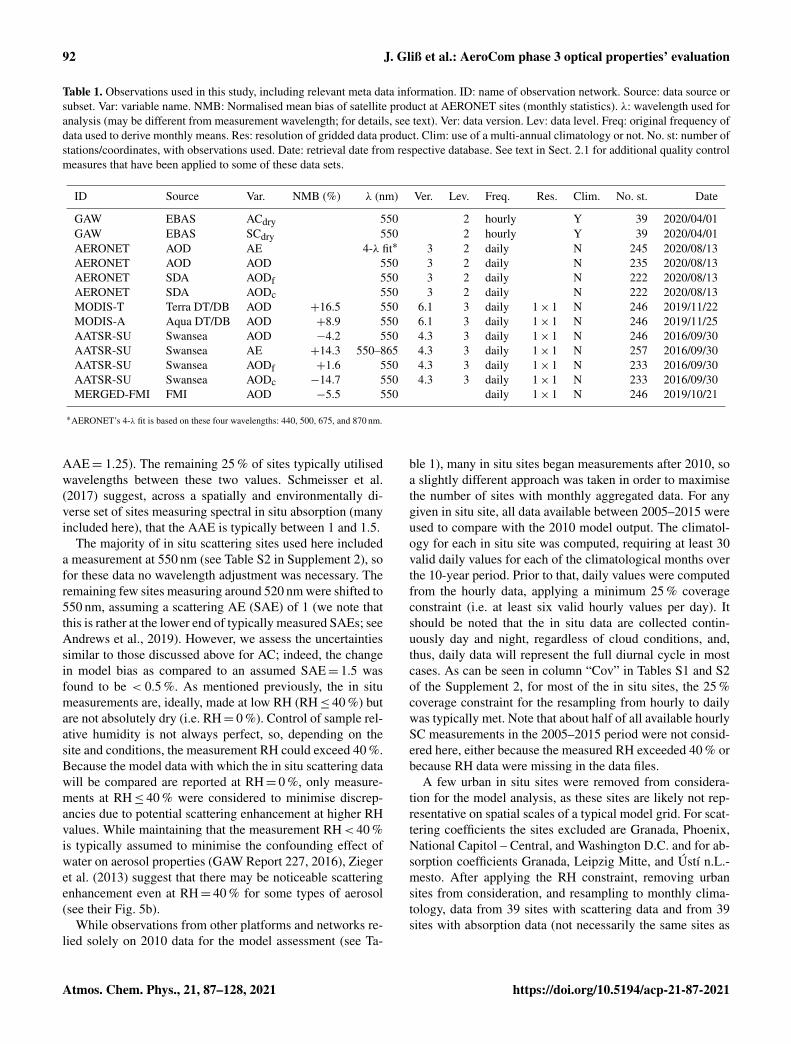
Table 1. Observations used in this study, including relevant meta data information. ID: name of observation network. Source: data source orsubset. Var: variable name. NMB: Normalised mean bias of satellite product at AERONET sites (monthly statistics). λ: wavelength used foranalysis (may be different from measurement wavelength; for details, see text). Ver: data version. Lev: data level. Freq: original frequency ofdata used to derive monthly means. Res: resolution of gridded data product. Clim: use of a multi-annual climatology or not. No. st: number ofstations/coordinates, with observations used. Date: retrieval date from respective database. See text in Sect. 2.1 for additional quality controlmeasures that have been applied to some of these data sets.
ID Source Var. NMB (%) λ (nm) Ver. Lev. Freq. Res. Clim. No. st. Date
GAW EBAS ACdry 550 2 hourly Y 39 2020/04/01GAW EBAS SCdry 550 2 hourly Y 39 2020/04/01AERONET AOD AE 4-λ fit∗ 3 2 daily N 245 2020/08/13AERONET AOD AOD 550 3 2 daily N 235 2020/08/13AERONET SDA AODf 550 3 2 daily N 222 2020/08/13AERONET SDA AODc 550 3 2 daily N 222 2020/08/13MODIS-T Terra DT/DB AOD +16.5 550 6.1 3 daily 1× 1 N 246 2019/11/22MODIS-A Aqua DT/DB AOD +8.9 550 6.1 3 daily 1× 1 N 246 2019/11/25AATSR-SU Swansea AOD −4.2 550 4.3 3 daily 1× 1 N 246 2016/09/30AATSR-SU Swansea AE +14.3 550–865 4.3 3 daily 1× 1 N 257 2016/09/30AATSR-SU Swansea AODf +1.6 550 4.3 3 daily 1× 1 N 233 2016/09/30AATSR-SU Swansea AODc −14.7 550 4.3 3 daily 1× 1 N 233 2016/09/30MERGED-FMI FMI AOD −5.5 550 daily 1× 1 N 246 2019/10/21
∗AERONET’s 4-λ fit is based on these four wavelengths: 440, 500, 675, and 870 nm.
AAE= 1.25). The remaining 25 % of sites typically utilisedwavelengths between these two values. Schmeisser et al.(2017) suggest, across a spatially and environmentally di-verse set of sites measuring spectral in situ absorption (manyincluded here), that the AAE is typically between 1 and 1.5.
The majority of in situ scattering sites used here includeda measurement at 550 nm (see Table S2 in Supplement 2), sofor these data no wavelength adjustment was necessary. Theremaining few sites measuring around 520 nm were shifted to550 nm, assuming a scattering AE (SAE) of 1 (we note thatthis is rather at the lower end of typically measured SAEs; seeAndrews et al., 2019). However, we assess the uncertaintiessimilar to those discussed above for AC; indeed, the changein model bias as compared to an assumed SAE= 1.5 wasfound to be < 0.5 %. As mentioned previously, the in situmeasurements are, ideally, made at low RH (RH≤ 40 %) butare not absolutely dry (i.e. RH= 0 %). Control of sample rel-ative humidity is not always perfect, so, depending on thesite and conditions, the measurement RH could exceed 40 %.Because the model data with which the in situ scattering datawill be compared are reported at RH= 0 %, only measure-ments at RH≤ 40 % were considered to minimise discrep-ancies due to potential scattering enhancement at higher RHvalues. While maintaining that the measurement RH< 40 %is typically assumed to minimise the confounding effect ofwater on aerosol properties (GAW Report 227, 2016), Ziegeret al. (2013) suggest that there may be noticeable scatteringenhancement even at RH= 40 % for some types of aerosol(see their Fig. 5b).
While observations from other platforms and networks re-lied solely on 2010 data for the model assessment (see Ta-
ble 1), many in situ sites began measurements after 2010, soa slightly different approach was taken in order to maximisethe number of sites with monthly aggregated data. For anygiven in situ site, all data available between 2005–2015 wereused to compare with the 2010 model output. The climatol-ogy for each in situ site was computed, requiring at least 30valid daily values for each of the climatological months overthe 10-year period. Prior to that, daily values were computedfrom the hourly data, applying a minimum 25 % coverageconstraint (i.e. at least six valid hourly values per day). Itshould be noted that the in situ data are collected contin-uously day and night, regardless of cloud conditions, and,thus, daily data will represent the full diurnal cycle in mostcases. As can be seen in column “Cov” in Tables S1 and S2of the Supplement 2, for most of the in situ sites, the 25 %coverage constraint for the resampling from hourly to dailywas typically met. Note that about half of all available hourlySC measurements in the 2005–2015 period were not consid-ered here, either because the measured RH exceeded 40 % orbecause RH data were missing in the data files.
A few urban in situ sites were removed from considera-tion for the model analysis, as these sites are likely not rep-resentative on spatial scales of a typical model grid. For scat-tering coefficients the sites excluded are Granada, Phoenix,National Capitol – Central, and Washington D.C. and for ab-sorption coefficients Granada, Leipzig Mitte, and Ústí n.L.-mesto. After applying the RH constraint, removing urbansites from consideration, and resampling to monthly clima-tology, data from 39 sites with scattering data and from 39sites with absorption data (not necessarily the same sites as
Atmos. Chem. Phys., 21, 87–128, 2021 https://doi.org/10.5194/acp-21-87-2021
J. Gliß et al.: AeroCom phase 3 optical properties’ evaluation 93
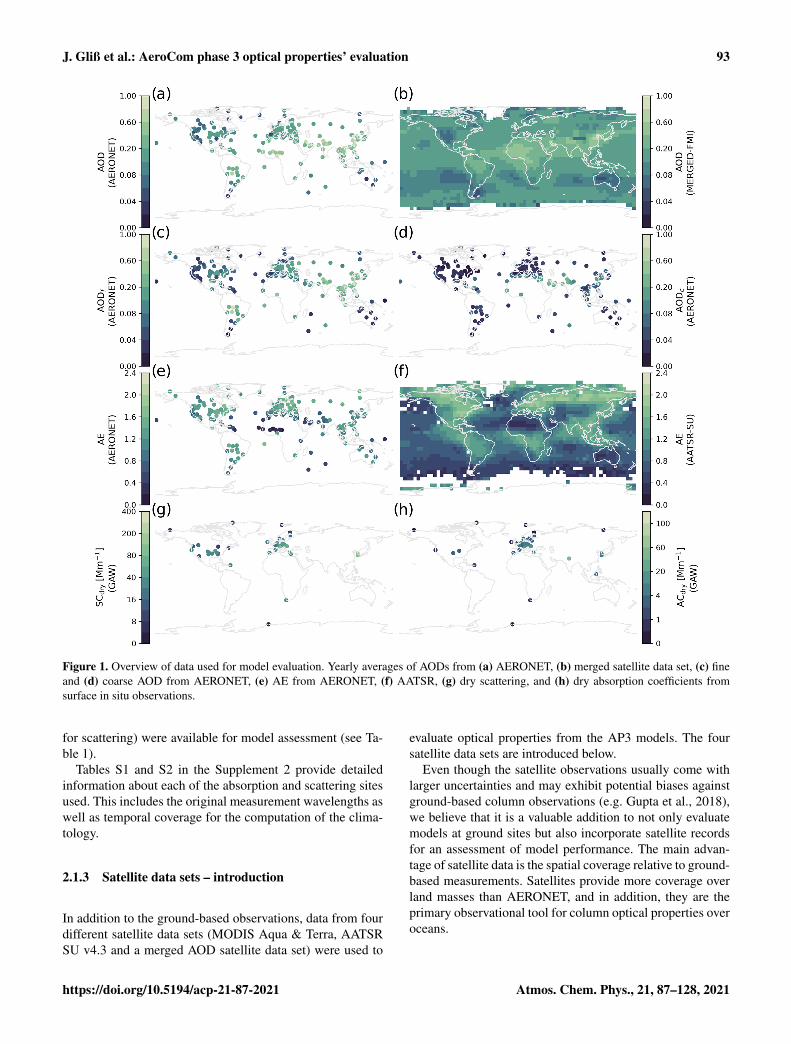
Figure 1. Overview of data used for model evaluation. Yearly averages of AODs from (a) AERONET, (b) merged satellite data set, (c) fineand (d) coarse AOD from AERONET, (e) AE from AERONET, (f) AATSR, (g) dry scattering, and (h) dry absorption coefficients fromsurface in situ observations.
for scattering) were available for model assessment (see Ta-ble 1).
Tables S1 and S2 in the Supplement 2 provide detailedinformation about each of the absorption and scattering sitesused. This includes the original measurement wavelengths aswell as temporal coverage for the computation of the clima-tology.
2.1.3 Satellite data sets – introduction
In addition to the ground-based observations, data from fourdifferent satellite data sets (MODIS Aqua & Terra, AATSRSU v4.3 and a merged AOD satellite data set) were used to
evaluate optical properties from the AP3 models. The foursatellite data sets are introduced below.
Even though the satellite observations usually come withlarger uncertainties and may exhibit potential biases againstground-based column observations (e.g. Gupta et al., 2018),we believe that it is a valuable addition to not only evaluatemodels at ground sites but also incorporate satellite recordsfor an assessment of model performance. The main advan-tage of satellite data is the spatial coverage relative to ground-based measurements. Satellites provide more coverage overland masses than AERONET, and in addition, they are theprimary observational tool for column optical properties overoceans.
https://doi.org/10.5194/acp-21-87-2021 Atmos. Chem. Phys., 21, 87–128, 2021
94 J. Gliß et al.: AeroCom phase 3 optical properties’ evaluation
Because of AERONET’s reliability and data quality, it isgenerally accepted as the gold standard for column AODmeasurements. Therefore, all four satellites used in this paperwere evaluated against AERONET data, in order to establishrelative biases and correlation coefficients. Details related tothis satellite assessment are discussed in Supplement 2 andare briefly mentioned in the introduction sections for eachindividual satellite below. The results from this satellite as-sessment are also available online (see Mortier et al., 2020a),allowing for an interactive exploration of the data and re-sults (down to the station level), and they include many eval-uation metrics (e.g. various biases, correlation coefficients,root mean square error (RMSE)). These comparisons of theindividual satellites against AERONET provide context forthe differences in the model assessments discussed below inSect. 4. It should be noted, however, that the retrieved biasesfor each satellite data set provide insights into the perfor-mance of each satellite product at AERONET sites, whichare land-dominated. Satellites often have different retrievalalgorithms over land and ocean (e.g. Levy et al., 2013), andthe aerosol retrieval tends to be more reliable over dark sur-faces, such as the oceans, than over bright surfaces, such asdeserts (e.g. Hsu et al., 2004).
2.1.4 MODIS data
Daily gridded level 3 AOD data from the Moder-ate Resolution Imaging Spectroradiometer (MODIS)have been used from both satellite platforms (Terraand Aqua) for evaluation of the models. Themerged land and ocean global product (namedAOD_550_Dark_Target_Deep_Blue_Combined_Meanin the product files) of the recent collection 6.1 was used.This is an updated and improved version of collection 6 (e.g.Levy et al., 2013; Sayer et al., 2014). For changes betweenboth data sets, see Hubanks (2017).
Details about the MODIS data sets used are provided inTable 1. Compared to AERONET, both Aqua and Terra ex-hibit positive AOD biases, suggesting an overestimation ofca. +9 % and +17 %, respectively, at AERONET sites andfor the year 2010 (for details, see Supplement 2). The largeroverestimate for Terra is in agreement with the findings fromHsu et al. (2004).
2.1.5 AATSR SU v4.3 data
The AATSR SU v4.3 data set provides gridded AOD and as-sociated parameters from the Advanced Along Track Scan-ning Radiometer (AATSR) instrument series, developed bySwansea University (SU) under the ESA Aerosol ClimateChange Initiative (CCI). The AATSR instrument on EN-VISAT covers the period 2002–2012, and in this study, datafrom 2010 are used. The instrument’s conical scan providestwo near-simultaneous views of the surface, at solar reflec-tive wavelengths from 555 nm to 1.6 µm.
Over land, the algorithm uses the dual-view capability ofthe instrument to allow estimation without a priori assump-tions on surface spectral reflectance (North, 2002; Bevanet al., 2012). Over ocean, the algorithm uses a simple modelof ocean surface reflectance including wind speed and pig-ment dependency at both nadir and along-track view angles.The retrieval directly finds an optimal estimate of both theAOD at 550 nm, and size, parameterised as relative propor-tions of fine- and coarse-mode aerosol. The local composi-tion of fine and coarse mode is adopted from the MACv1aerosol climatology (Kinne et al., 2013). The local coarsecomposition is defined by fractions of non-spherical dust andlarge spherical particles typical of sea salt aerosol, while finemode is defined by relative fractions of weak and strong ab-sorbing aerosol. A full description of these component mod-els is given in de Leeuw et al. (2015). Further aerosol prop-erties including AE (calculated between 550 and 856 nm)and absorption aerosol optical depth (AAOD; not used inthis study) are determined from the retrieved AOD and com-position. Aerosol properties are retrieved over all snow-freeand cloud-free surfaces. The most recent version AATSR SUV4.3 (North and Heckel, 2017) advances on previous ver-sions by improved surface modelling and shows reduced pos-itive bias over bright surfaces. Retrieval uncertainty and com-parison with sun photometer observations show highest accu-racy retrieval over ocean and darker surfaces, with higher un-certainty over bright surfaces (e.g. desert, snow) and for largezenith angles (Popp et al., 2016). This study uses the level3 output, which is provided at daily and monthly 1◦× 1◦
resolution, intended for climate model comparison. Specif-ically, AATSR SU values for AE and total, fine, and coarseAODs are used. The AE calculation is only performed for0.05<AOD< 1.5 due to increased retrieval uncertainty ofAE at low and high AODs.
In comparison with AERONET, the AATSR data exhibitan AOD bias of ∼−4 %, suggesting a slight underestima-tion of AOD at AERONET sites, in contrast to the twoMODIS products used (see Table 1). To our knowledge, thisAATSR product (SU V4.3) has not been evaluated againstAERONET in the literature. Thus, these results comprise animportant finding of this study. Biases of AODf, AODc, andAE against AERONET were found to be +1.6 %, −14.7 %,and +14.3 %, respectively (see web visualisation; Mortieret al., 2020a).
Initial comparisons within the CCI Aerosol project sug-gest that the fine-mode fraction of total AOD may be overes-timated over the ocean, with consequently some high bias inAE. The AE provided by AATSR is estimated for the range550–870 nm, and some difference may also be expected withAERONET-derived AE using a different wavelength range(e.g. Schuster et al., 2006).
Atmos. Chem. Phys., 21, 87–128, 2021 https://doi.org/10.5194/acp-21-87-2021
J. Gliß et al.: AeroCom phase 3 optical properties’ evaluation 95
2.1.6 Merged satellite AOD data
The MERGED-FMI data set, developed by the Finnish Me-teorological Institute, includes gridded level 3 monthly AODproducts merged from 12 available satellite products (So-gacheva et al., 2020). It should be noted that MODIS andAATSR products are considered inside this MERGED-FMIdata set. It is available for the period 1995–2017; however,here only 2010 data are used.
Compared to AERONET measurements from 2010, thismerged satellite product has shown excellent performancewith the highest correlation (R = 0.89) among the four satel-lites used and only a slight underestimation of AOD (bias of−5.4 %) at AERONET sites (see Supplement 2 and Mortieret al., 2020a). The merging method is based on the re-sults of the evaluation of the individual satellite AOD prod-ucts against AERONET. These results were utilised to in-fer a regional ranking, which was then used to calculate aweighted AOD mean. Because it is combined from the in-dividual products of different spatial and temporal resolu-tion, the AOD merged product is characterised by the bestpossible coverage, compared with other individual satelliteproducts. The AOD merged product is at least as capableof representing monthly means as the individual products(Sogacheva et al., 2020). Standard pixel-level uncertaintiesfor the merged AOD product were estimated as the rootmean squared sum of the deviations between that productand eight other merged AOD products calculated with dif-ferent merging approaches applied for different aerosol types(Sogacheva et al., 2020).
2.1.7 Global distribution of optical propertiesinvestigated
The previous sections introduced the individual ground- andspace-based observation records and optical properties vari-ables that will be used in this paper for the model assess-ment. Figure 1 provides an overview of the global distribu-tion of these optical properties. The global maps displayedshow annual mean values of all variables considered, bothfor the ground-based networks and for a selection of thesatellite observations. Figure 1a, c, and d show yearly av-erage mean values of the observed AERONET AODs (total,coarse, and fine, respectively). Column Ångström exponentsfrom AERONET are shown in Fig. 1e. Dust-dominated re-gions such as northern Africa and south-west Asia are clearlyvisible both in the coarse AOD and the AE but also in thetotal AOD, indicating the importance of dust for the globalAOD signal. The satellite observations of AOD (MERGED-FMI) and AE (ATSR-SU) (Fig. 1b, f) are particularly use-ful in remote regions and over the oceans, where ground-based measurements are less common. Thus, they add sub-stantially to the global picture when assessing models. Forexample, satellites capture the nearly constant AOD back-ground of around 0.1 over the ocean (mostly arising from
sea salt) which cannot be obtained from the land-dominated,ground-based observation networks. The AE from AATSR-SU shows a latitudinal southwards decreasing gradient in re-mote ocean regions, indicating dominance of coarse(r) parti-cle size distributions, which is likely due to cleaner and, thus,more sea-salt-dominated regions. Transatlantic dust transportresults in an increased particle size west of the Sahara (e.g.Kim et al., 2014) as is captured by AATSR-SU. Finally, itis difficult to observe global patterns in the in situ scatter-ing and absorption data due to the limited spatial coverageof the measurements, as can be seen in the lowermost panels(Fig. 1g, h). The differences in the spatial coverage for eachobservation data set will be important to keep in mind wheninterpreting the results presented in Sect. 4.
2.2 Models
This study uses output from 14 models that are participatingin the AeroCom AP3-CTRL experiment. Details on the Ae-roCom phase III experiments can be found on the AeroComwiki page (AeroCom wiki, 2020). The wiki also includes in-formation on how to access the model data from the differ-ent AeroCom phases and experiments, which are stored inthe AeroCom database. Note that the database location andinformation about it might change in the future; the inten-tion is however to keep updated information available viathe website: https://aerocom.met.no (last access: 14 Septem-ber 2020). Table 2 provides an overview of the models usedin this paper. For the AP3-CTRL experiment, modellers wereasked to submit simulations of at least the years 2010 and1850, with 2010 meteorology and prescribed (observed) seasurface temperature and sea ice concentrations, and usingemission inventories from CMIP6 (Eyring et al., 2016), whenpossible. Details concerning the anthropogenic and biomassburning emissions are given in the Community EmissionsData System (CEDS; Hoesly et al., 2018) and in biomassburning emissions for CMIP6 (BB4CMIP; van Marle et al.,2017). In this paper, only the 2010 model output is used. Theyear 2010 was chosen as a reference year by the AeroComconsortium and is used throughout many phase II and IIIexperiments for the inter-comparability of different experi-ments and model generations. The AeroCom phase I simula-tions (e.g. Dentener et al., 2006; Kinne et al., 2006; Schulzet al., 2006; Textor et al., 2006) used the year 2000 as a ref-erence year. One of the main reasons to update the referenceyear from 2000 to 2010 was that many more observationsbecame available between 2000 and 2010 and also to ac-count for changes in the present-day climate, for instance,due to changing emissions and composition (e.g. Klimontet al., 2013; Aas et al., 2019; Mortier et al., 2020b).
Detailed information about the models on emissions, hu-midity growth, and particularly their treatment of aerosol op-tics has been collected from the modelling groups through aquestionnaire. The tabulated responses are provided in Sup-plement 1. The first table (spreadsheet “Table: General ques-
https://doi.org/10.5194/acp-21-87-2021 Atmos. Chem. Phys., 21, 87–128, 2021
96 J. Gliß et al.: AeroCom phase 3 optical properties’ evaluation
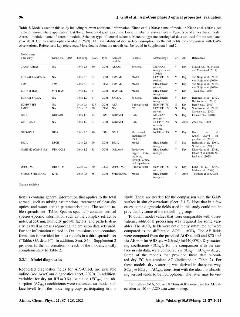
Table 2. Models used in this study including relevant additional information. Kinne et al. (2006): name of model in Kinne et al. (2006) (seeTable 2 therein, where applicable). Lat./long.: horizontal grid resolution. Levs.: number of vertical levels. Type: type of atmospheric model.Aerosol module: name of aerosol module. Scheme: type of aerosol scheme. Meteorology: meteorological data set used for the simulatedyear 2010. CS: clear-sky optics available (Y/N). AC: availability of dry surface absorption coefficient fields for comparison with GAWobservations. References: key references. More details about the models can be found in Supplement 1 and 2.
Model nameThis study Kinne et al. (2006) Lat./long. Levs. Type Aerosol
moduleScheme Meteorology CS AC References
CAM5-ATRAS NA 1.9× 2.5 30 GCM ATRAS Sectional MERRA2(nudged, above800 hPa)
Y Dry Matsui (2017), Matsuiand Mahowald (2017)
EC-Earth3-AerChem NA 2.0× 3.0 34 GCM TM5-M7 Modal ECMWF-IFS(online)
Y Dry van Noije et al. (2014),van Noije et al. (2020)
TM5 TM5 2.0× 3.0 34 CTM TM5-M7 Modal ERA-Interim(driven)
Y Dry van Noije et al. (2014),van Noije et al. (2020)
ECHAM-HAM MPI-HAM 1.9× 1.9 47 GCM HAM-M7 Modal ERA-Interim(nudged)
Y Dry Tegen et al. (2019)
ECHAM-SALSA NA 1.9× 1.9 47 GCM SALSA Sectional ERA-Interim(nudged)
Y Dry Bergman et al. (2012),Kokkola et al. (2018)
ECMWF-IFS NA 0.4× 0.4 137 GCM AER Bulk/sectional ECMWF-IFS N Dry Rémy et al. (2019)EMEP NA 0.5× 0.5 20 CTM NA NA ECMWF-IFS
(driven)N Dry Simpson et al. (2012),
Schulz et al. (2012)GEOS GOCART 1.0× 1.0 72 ESM GOCART Bulk MERRA2
(nudged)N Dry Colarco et al. (2010),
GFDL-AM4 NA 1.0× 1.2 33 GCM GOCART Bulk NCEP-NCARre-analysis(nudged)
N Amb. Zhao et al. (2018)
GISS-OMA GISS 2.0× 2.5 40 ESM OMA Mass-based,sectional forSS & DU
NCEP-NCAR Y Dry Koch et al.(2006, 2007), Tsi-garidis et al. (2013)
INCA LSCE 1.3× 2.5 79 GCM INCA Modal ERA-Interim(nudged)
Y NA Balkanski et al. (2004),Schulz et al. (2009)
NorESM2 (CAM6-Nor) UIO_GCM 0.9× 1.2 32 GCM OsloAero Production-tagged (size-resolvingthrough offlinelook-up tables)
ERA-Interim(nudged)
Y Dry Kirkevåg et al. (2018),Olivié et al. (2020), Se-land et al. (2020)
OsloCTM3 UIO_CTM 2.2× 2.2 60 CTM OsloCTM3 Bulk/sectional ECMWF-IFS(driven)
N Dry Lund et al. (2018),Myhre et al. (2009)
MIROC-SPRINTARS KYU 0.6× 0.6 56 GCM SPRINTARS Modal ERA-Interim(nudged)
Y Amb. Takemura et al. (2005)
NA: not available
tions”) contains general information that applies to the totalaerosol, such as mixing assumptions, treatment of clear-skyoptics, and water uptake parameterisations. The second ta-ble (spreadsheet “Table: Species-specific”) contains aerosolspecies-specific information such as the complex refractiveindex at 550 nm, humidity growth factors, and particle den-sity, as well as details regarding the emission data sets used.Further information related to OA emissions and secondaryformation is provided for most models in a third spreadsheet(“Table: OA details”). In addition, Sect. S4 of Supplement 2provides further information on each of the models, mostlycomplementary to Table 2.
2.2.1 Model diagnostics
Requested diagnostics fields for AP3-CTRL are availableonline (see AeroCom diagnostics sheet, 2020). In addition,variables for dry (at RH= 0 %) extinction (ECdry) and ab-sorption (ACdry) coefficients were requested (at model sur-face level) from the modelling groups participating in this
study. These are needed for the comparison with the GAWsurface in situ observations (Sect. 2.1.2). Note that in a fewcases, some diagnostic fields used in this study could not beprovided by some of the modelling groups.
To obtain model values that were comparable with obser-vations, additional processing was required for some vari-ables. The AODc fields were not directly submitted but werecomputed as the difference: AOD – AODf. The AE fieldswere computed from the provided AOD at 440 and 870 nm2
via AE=− ln(AOD440/AOD870)/ ln(440/870). Dry scatter-ing coefficients (SCdry), for the comparison with the sur-face in situ data, were computed via SCdry =ECdry−ACdry.Some of the models that provided these data submit-ted dry EC but ambient AC (indicated in Table 2). Forthese models, dry scattering was derived in the same way,SCdry =ECdry−ACamb, consistent with the idea that absorb-ing aerosol tends to be hydrophobic. The latter may be vio-
2For GISS-OMA, 550 and 870 nm AODs were used for AE cal-culation as 440 nm AOD data were missing.
Atmos. Chem. Phys., 21, 87–128, 2021 https://doi.org/10.5194/acp-21-87-2021

J. Gliß et al.: AeroCom phase 3 optical properties’ evaluation 97
lated to some degree for models that include internally mixedBC modes with hydrophilic species, such as SO4. However,an investigation of differences between dry and ambient ab-sorption coefficients revealed that the overall impact on theresults is minor, both for models with internally mixed BCmodes and for models with externally mixed modes.
Some of the models reported the columnar optical prop-erties based on clear-sky (CS) assumptions, while othersassumed all-sky (AS) conditions to compute hygroscopicgrowth and extinction efficiencies. These choices are indi-cated in Table 2, and details related to the computation of CSoptics can be found in Supplement 1.
The following modelled global average values have beenretrieved of species-specific model parameters to be com-pared in Sect. 3 in order to assess life cycle aspects of modeldiversity:
1. Emissions and formation of aerosol species were re-trieved (in units of Tg/year). The secondary aerosol for-mation of SO4, NO3, and OA by chemical reactions inthe atmosphere is difficult to diagnose. Thus, it is diag-nosed here from total deposition output.
2. Lifetimes of major aerosol species (in units of days)were computed from column burden and providedwet+dry deposition rates. The lifetimes can give in-sights into the efficiency of removal processes in themodels.
3. Global mass burdens were provided (in units of Tg) foreach species. These values enable comparisons amongstthe models in terms of aerosol amount present on aver-age.
4. Modelled speciated optical depths (ODs) at 550 nmwere provided. This unitless quantity provides anotherway of looking at contributions from different species tototal AOD based on their optical properties rather thantheir burden.
5. Modelled mass extinction coefficients (MECs, in unitsof m2/g) at 550 nm were calculated for each species bydividing the species optical depth by the correspondingspecies mass burden (e.g. ODDU/LOADDU). The MECdetermines the conversion of aerosol mass to light ex-tinction and can provide insights into the variability ofmodelled size distributions or hygroscopicity.
6. Additionally, modelled mass absorption coefficients(MACs) at 550 nm for light-absorbing species (BC,DU, organic carbon (OC)) were calculated by di-viding the species absorption optical depth (AAOD)by the corresponding species mass burden (e.g.AAODBC/LOADBC).
We note again that detailed introductions for each modelare provided in Supplement 1 and in Sect. S4 of Supplement2, in addition to the summary in Table 2.
2.3 Data processing and statistics
Most of the analysis in this study was per-formed with the software pyaerocom (Zenodo:https://doi.org/10.5281/zenodo.4362479, Gliß et al.,2020). pyaerocom is an open-source Python software projectthat is being developed and maintained for the AeroCominitiative, at the Norwegian Meteorological Institute. Itprovides tools for the harmonisation and co-location ofmodel and observation data and dedicated algorithms for theassessment of model performance at all scales. Evaluationresults from different AeroCom experiments are uploadedto a dedicated website that allows exploration of the modeland observation data and evaluation metrics. The websiteincludes interactive visualisations of performance charts(e.g. biases, correlation coefficients), scatter plots, biasmaps, and individual station and regional time series data,for all models and observation variables, as well as bar chartssummarising regional statistics. All results from the opticalproperties’ evaluation discussed in this paper are availablevia a web interface (see Mortier et al., 2020c).
The ground- and space-based observations are co-locatedwith the model simulations by matching them with the clos-est model grid point in the model resolution originally pro-vided.
In the case of ground-based observations (AERONET andGAW in situ), the model grid point closest to each mea-surement site is used. For the satellite observations, both themodel data and the (gridded) satellite product are re-griddedto a resolution of 5◦×5◦, and the closest model grid point toeach satellite pixel is used. The choice of this rather coarseresolution is a compromise, mostly serving the purpose of in-creasing the temporal representativity (i.e. more data pointsper grid cell) in order to meet the time resampling constraints(defined below). For the comparison of satellite AODs withmodels, a minimum AOD of 0.01 was required, due to theincreased uncertainties related to satellite AOD retrievals atlow column burdens. The low AODs were filtered in the orig-inal resolution of the level 3 gridded satellite products, priorto the co-location with the models.
Since many model fields were only available in monthlyresolution, the co-location of the data with the observations(and the computation of the statistical parameters used tocompare the models) was performed in monthly resolution.Any model data provided in higher temporal resolution wereaveraged to obtain monthly mean values, prior to the analy-sis. For the higher resolution observations (see Table 1), thecomputation of monthly means was done using a hierarchi-cal resampling scheme, requiring at least ∼ 25 % coverage.Practically, this means that the daily AERONET data wereresampled to a monthly scale, requiring at least seven dailyvalues in each month. For the hourly in situ data, first a dailymean was computed (requiring at least six valid hourly val-ues), and from these daily means, monthly means were com-
https://doi.org/10.5194/acp-21-87-2021 Atmos. Chem. Phys., 21, 87–128, 2021
98 J. Gliß et al.: AeroCom phase 3 optical properties’ evaluation
puted, requiring at least seven daily values. Data that did notmatch these coverage constraints were invalidated.
Throughout this paper, the discussion of the results willuse two statistical parameters to assess the model perfor-mance: the normalised mean bias (NMB) is defined as
NMB =∑Ni (mi−oi )∑N
i oi, where mi and oi are the model and ob-
servational mean, respectively, and the Pearson correlationcoefficient (R). More evaluation metrics, such as normalisedRMSE or fractional gross error, are available online in theweb visualisation (Mortier et al., 2020c) but are not furtherconsidered within this paper.
Section 4.5 presents several sensitivity studies that wereperformed in order to investigate the spatio-temporal rep-resentativity of this analysis strategy, which is based onnetwork-averaged, monthly aggregates. This was done be-cause representativity (or lack thereof) comprises a majorsource of uncertainty (e.g. Schutgens et al., 2016, 2017;Sayer and Knobelspiesse, 2019). The focus here was to as-sess how such potential representation errors affect the biasesand correlation coefficients used in this paper to assess themodel performance and comparison with other models.
2.3.1 AeroCom ensemble mean and median
For all variables investigated in this paper, the monthly Ae-roCom ensemble mean (ENS-MEAN) and median (ENS-MED) fields were computed and have been made available inthe AeroCom database, for future reference. This was donein order to enable an assessment of the AP3 model ensem-ble, which we consider to represent the most likely modellingoutput of the state-of-the-art aerosol model versions partici-pating in the AP3-CTRL exercise.
The ensemble fields were computed in a latitude–longitude resolution of 2◦×3◦, which corresponds to the low-est available model resolution (i.e. of models EC-Earth andTM5; see Table 2). Model fields were all re-gridded to thisresolution before the ensemble mean and median were com-puted. In this paper, only the output from the median modelis used. Note that results from the mean model are not fur-ther discussed below but are available online (see Mortieret al., 2020c). In addition to the median (50th percentile), the25th (Q1) and 75th (Q3) percentiles were also computed andevaluated against the observations like any other model. Thiswas done to enable an assessment of model diversity in theretrieved biases and correlation coefficients.
In addition, local diversity fields were computed for eachvariable by dividing the interquartile range (IQR=Q1–Q3)by the ensemble median: δIQR= IQR/median, which corre-sponds to the central 50 % of the models as a measure of di-versity (this is different than Kinne et al., 2006, who use thecentral 2/3). Note that the IQR is not necessarily symmetricalwith respect to the median. In order to enable a better com-parison with the AP1 results from Textor et al. (2006) andKinne et al. (2006), a second set of diversity fields was com-
puted as follows: δstd = σ/ (ensemble mean), where σ is thestandard deviation.
Note that the ensemble AE fields were computed from theindividual models’ AE fields. In the case of the ensemblemedian, this will give slightly different results compared to acomputation of a median based on median 440 and 870 AODfields. This is because the median computation is done in AEspace and not in AOD space.
Please also note that the ensemble total AOD includes re-sults from INCA which are not included in AODf and AODc.This results in a slightly smaller total AOD in the ensemblewhen inferred from AODf+AODc (which does not includeINCA) compared to the computed AOD field (which includesINCA).
2.3.2 Model STP correction for comparison with GAWin situ data
Since the GAW in situ measurements are reported at STPconditions (Sect. 2.1.2), the 2010 monthly model data wereconverted to STP using the following formula:
XSTP =Xamb×
(Pstd
Pamb
)·
(Tamb
Tstd
). (1)
XSTP and Xamb are the model value of absorption (or scat-tering) at STP and ambient conditions, respectively. Pamb andTamb are the ambient air pressure and temperature at the cor-responding site location. The correction factor was estimatedon a monthly basis, where Pamb was estimated based on thestation altitude (using the barometric formula and assuminga standard atmosphere implemented in the python geonumlibrary; Gliß, 2017), and Tamb was estimated using monthlynear-surface (2 m) temperature data from ERA5 (2019). Thiscorrection may introduce some statistic error, mostly due tonatural fluctuations in the pressure and possible uncertaintiesin the ERA5 temperature data. However, we assess this addi-tional uncertainty to be small for the annual average statisticsdiscussed below.
3 Results and discussion – model diversity of aerosollife cycle and optical properties
The focus of this section is to establish a global picture and totry to understand model diversity in relevant parameters re-lated to the aerosol life cycle (i.e. global emissions, lifetimes,and burdens) as well as the simulated aerosol optical proper-ties (i.e. speciated MECs, MACs, and ODs). The goal is todevelop an understanding of how, based on the models, pro-cesses and parameterisations link emissions to optical prop-erties. A comparison of modelled optical properties with thevarious observation records is presented in Sect. 4.
Most of the discussion in this section focuses on themodel ensemble median and associated diversities (δIQR).Section 3.1 focuses on diversity in the treatment of the differ-ent aerosol species in the models, starting with an overview
Atmos. Chem. Phys., 21, 87–128, 2021 https://doi.org/10.5194/acp-21-87-2021
J. Gliß et al.: AeroCom phase 3 optical properties’ evaluation 99
of simulated global aerosol emissions, lifetimes, and massburdens (Sect. 3.1.1), followed by a discussion of simulatedODs, MECs, and MACs for each species (Sect. 3.1.2). Sec-tion 3.2 provides and discusses the global distribution of thesimulated aerosol optical properties and their spatial diver-sity.
3.1 Life cycle and optical properties for each aerosolspecies
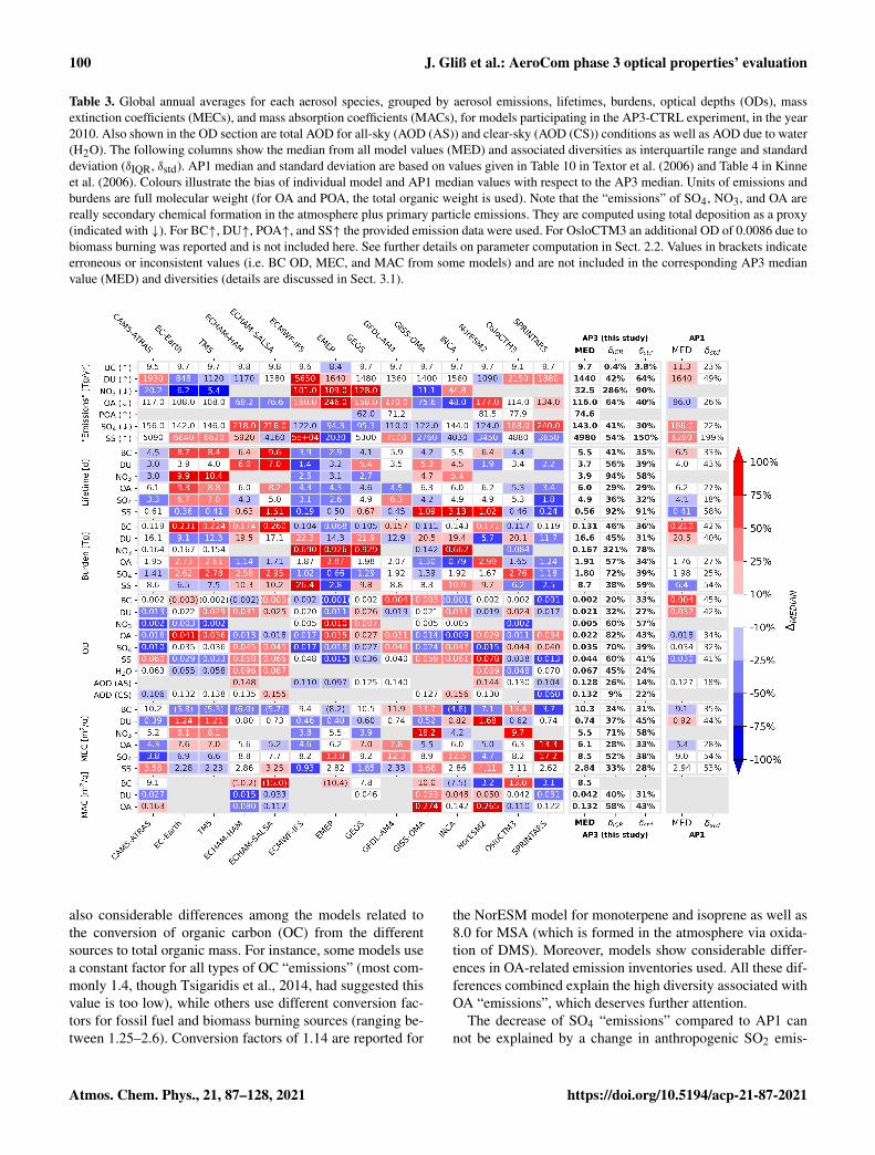
Table 3 provides an overview of global annual mean values ofemissions, lifetimes, burdens, ODs, MECs, and, where avail-able, MACs, for each aerosol species (i.e. BC, DU, NO3, OA,SO4, and SS) and for each model. Gaps in the table indicatewhere models did not provide a requested variable. Also in-cluded are the median (MED) and diversity estimates (δIQR,δstd) for each species and variable. Note that these are com-puted directly from the values provided in Table 3, not usingthe ensemble median fields. For comparison, median and δstdfrom the AeroCom phase 1 (AP1) simulations are providedas well. The colours in the table provide an indication of thesign and bias of the individual model values relative to theAP3 median.
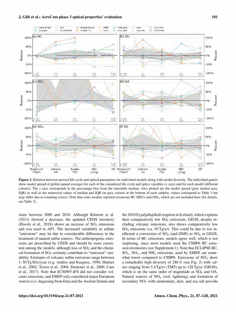
Figure 2 provides a different view of the data provided inTable 3, by illustrating how the diversity of the individualparameters contributes to the resulting model ensemble di-versity in species OD, similar to illustrations used earlier inSchulz et al. (2006) (their Fig. 8) and Myhre et al. (2013)(their Fig. 14). This visualisation makes it easier to link thediversity in speciated ODs with the uncertainty in modellingthe processes controlling the OD of each species.
3.1.1 Aerosol life cycle: from emissions to massburdens
As explained above, global aerosol emission and formation(in Table 3) were estimated either using the provided emis-sion fields, as for primary aerosols BC, DU, SS, and POA(primary organic aerosol), or using the equivalent total emis-sions, as for SO4, OA, and NO3 based on total deposition.For simplicity we also call the equivalent total emissions,which include secondary formation from precursors, “emis-sions” in this section. Note, that only major aerosol speciesare included in our study; aerosol precursor species that areprovided by some few models (e.g. NOx, NH4, or VOCs) arenot analysed.
Emissions are highest for sea salt (4980 Tg/yr), followedby dust (1440 Tg/yr), SO4 (143 Tg/yr), OA (116 Tg/yr, ofwhich ca. 75 Tg/yr is due to primary emissions), NO3(33 Tg/yr), and BC (10 Tg/yr). Compared to AP1, the me-dian emissions have decreased for all species except organicaerosols. For prescribed anthropogenic emissions, the differ-ences between AP1 and AP3 may partly be due to differencesin the emissions inventories. AP1 used inventories for theyear 2000, whereas, here, the 2010 emissions are used (for
details, see Supplement 1, Sect. S6). Differences are likelyalso due to changes in the modelling setups and emission pa-rameterisations.
Changes in parameterisations of online calculated naturalDU and SS emissions are an explanation for their decreasedemissions, 12 % and 21 %, respectively, compared to AP1.DU diversity has increased slightly relative to AP1, while SSdiversity has decreased; however, with a standard deviationof ca. 150 %, it is still very large. As in AP1, the reasons fordiversity in DU and SS emissions can be found in a rangeof parameters: surface winds, regions available to act as asource (semi-arid and arid areas for DU, sea-ice-free oceanfor SS), power functions used in the wind–emission relation-ship, aerosol size, and other factors. As an example, differentsize cut-offs are applied in the models when computing thesource strength (see Sect. 2.2). For instance, EMEP includesdust particles with sizes up to 10 µm, and TM5 and EC-Earthconsider sizes up to 16 µm, while ECMWF-IFS considerssizes up to 20 µm. While the higher size cut explains higheremissions for the IFS model, it does not explain why the TM5dust emissions are lower than those in the EMEP model.
The emission strengths of dust and sea salt reflect the sur-face wind distribution, which exhibits a larger tail in the dis-tribution at higher resolution and in free-running atmosphericmodels. Meteorological nudging that was required for AP3-CTRL leads to lower emissions (e.g. Timmreck and Schulz,2004). Most of the models in the AP1 simulations imple-mented free-running atmospheric models but operated atlower resolution, which should cancel out to a certain degreeand make AP1 and AP3 similar when it comes to effectivesurface wind distribution. Better documented wind distribu-tions could help explain emission differences. For instance,SPRINTARS (one of the highest resolution models; see Ta-ble 2) exhibits a negative departure from the median in SSemissions but an above-average DU source (ca. 1900 Tg/yr).The latter is comparable to that of OsloCTM3 and EMEP,which both use reanalysis winds at different resolutions. Alsonoteworthy are considerable differences in SS emissions be-tween the two ECHAM models (ECHAM-SALSA emits ca.30 % less SS but 18 % more dust than ECHAM-HAM), eventhough these two models use the same emission parameteri-sation (see Sect. S4 in Supplement 2) and the same meteorol-ogy for nudging and have the same resolution (see Table 2).This indicates that nudging and higher resolution in AP3 arenot the sole explanation for the AP3 decrease in the dust andsea salt emission strengths against AP1 and that inconsisten-cies remain.
Considerable diversity is also observed for OA emissions(64 %), which is a result of multiple organic aerosol sources,represented differently by the models (Supplement 1). Un-certainties are associated with the primary organic parti-cle emissions (POA; diagnosed in only four models), bio-genic and anthropogenic secondary organic aerosol forma-tion (SOA), and DMS-derived MSA, as well as biomassburning sources. As can be seen in Supplement 1, there are
https://doi.org/10.5194/acp-21-87-2021 Atmos. Chem. Phys., 21, 87–128, 2021
100 J. Gliß et al.: AeroCom phase 3 optical properties’ evaluation
Table 3. Global annual averages for each aerosol species, grouped by aerosol emissions, lifetimes, burdens, optical depths (ODs), massextinction coefficients (MECs), and mass absorption coefficients (MACs), for models participating in the AP3-CTRL experiment, in the year2010. Also shown in the OD section are total AOD for all-sky (AOD (AS)) and clear-sky (AOD (CS)) conditions as well as AOD due to water(H2O). The following columns show the median from all model values (MED) and associated diversities as interquartile range and standarddeviation (δIQR, δstd). AP1 median and standard deviation are based on values given in Table 10 in Textor et al. (2006) and Table 4 in Kinneet al. (2006). Colours illustrate the bias of individual model and AP1 median values with respect to the AP3 median. Units of emissions andburdens are full molecular weight (for OA and POA, the total organic weight is used). Note that the “emissions” of SO4, NO3, and OA arereally secondary chemical formation in the atmosphere plus primary particle emissions. They are computed using total deposition as a proxy(indicated with ↓). For BC↑, DU↑, POA↑, and SS↑ the provided emission data were used. For OsloCTM3 an additional OD of 0.0086 due tobiomass burning was reported and is not included here. See further details on parameter computation in Sect. 2.2. Values in brackets indicateerroneous or inconsistent values (i.e. BC OD, MEC, and MAC from some models) and are not included in the corresponding AP3 medianvalue (MED) and diversities (details are discussed in Sect. 3.1).
also considerable differences among the models related tothe conversion of organic carbon (OC) from the differentsources to total organic mass. For instance, some models usea constant factor for all types of OC “emissions” (most com-monly 1.4, though Tsigaridis et al., 2014, had suggested thisvalue is too low), while others use different conversion fac-tors for fossil fuel and biomass burning sources (ranging be-tween 1.25–2.6). Conversion factors of 1.14 are reported for
the NorESM model for monoterpene and isoprene as well as8.0 for MSA (which is formed in the atmosphere via oxida-tion of DMS). Moreover, models show considerable differ-ences in OA-related emission inventories used. All these dif-ferences combined explain the high diversity associated withOA “emissions”, which deserves further attention.
The decrease of SO4 “emissions” compared to AP1 cannot be explained by a change in anthropogenic SO2 emis-
Atmos. Chem. Phys., 21, 87–128, 2021 https://doi.org/10.5194/acp-21-87-2021
J. Gliß et al.: AeroCom phase 3 optical properties’ evaluation 101
Figure 2. Relation between aerosol life cycle and optical parameters for individual models along with model diversity. The individual panelsshow model spread of global annual averages for each of the considered life cycle and optics variables (x axis) and for each model (differentcolours). The y axis corresponds to the percentage bias from the ensemble median. Also plotted are the model spread (grey shaded area,IQR) as well as the numerical values of median and IQR (in grey colours at the bottom of each subplot; values correspond to Table 3 butmay differ due to rounding errors). Note that some models reported erroneous BC MECs and ODs, which are not included here (for details,see Table 3).
sions between 2000 and 2010. Although Klimont et al.(2013) showed a decrease, the updated CEDS inventory(Hoesly et al., 2018) shows an increase of SO2 emissionsand was used in AP3. The increased variability in sulfate”emissions” may be due to considerable differences in thetreatment of natural sulfur sources. The anthropogenic emis-sions are prescribed by CEDS and should be more consis-tent among the models, although loss of SO2 and the chemi-cal formation of SO4 certainly contribute to “emission” vari-ability. Estimates of volcanic sulfur emissions range between1–50 Tg SO2/year (e.g. Andres and Kasgnoc, 1998; Halmeret al., 2002; Textor et al., 2004; Dentener et al., 2006; Carnet al., 2017). Note that ECMWF-IFS did not consider vol-canic emissions, and EMEP only considered major Europeansources (i.e. degassing from Etna and the Aeolian Islands and
the 2010 Eyjafjallajökull eruption in Iceland), which explainstheir comparatively low SO4 emissions. GEOS, despite in-cluding volcanic emissions, also shows comparatively lowSO4 emissions (ca. 95 Tg/yr). This could be due to too in-efficient a conversion of SO2 (and DMS) to SO4 in GEOS.In terms of BC emissions, models agree well, which is notsurprising, since most models used the CMIP6 BC emis-sion inventories (see Supplement 1). Note that ECLIPSE BC,SOx , NOx , and NH3 emissions, used by EMEP, are some-what lower compared to CMIP6. Emissions of NO3 showa remarkably high diversity of 286 % (see Fig. 2) with val-ues ranging from 5.4 Tg/yr (TM5) up to 128 Tg/yr (GEOS),which is on the same order of magnitude as SO4 and OA.Natural sources of NOx (soil, lightning) and formation ofsecondary NO3 with ammonium, dust, and sea salt provide
https://doi.org/10.5194/acp-21-87-2021 Atmos. Chem. Phys., 21, 87–128, 2021
102 J. Gliß et al.: AeroCom phase 3 optical properties’ evaluation
several degrees of freedom for model formulation. NO3 hasonly been implemented in some models in recent years andwas not considered in the AP1 simulations.
The lifetimes (computed from burden and total deposition)are shown in the second panel in Table 3. Associated diversi-ties are illustrated in Fig. 2. OA has the longest lifetime with6 d, followed by BC (5.5 d), SO4 (4.9 d), NO3 (3.9 d), DU(3.7 d), and SS (0.56 d). The largest differences compared toAP1 are found for BC, which shows a decrease in lifetimeof ca. 15 %, and in SO4 and SS, showing increased lifetimesof ca. 20 % and 37 %, respectively. In addition, the latter twospecies show a notable increase in lifetime diversity com-pared to AP1. In the case of sulfate, the increased variabil-ity is in agreement with the changes in emissions discussedabove (i.e. it may reflect an increase in the natural fraction).This is consistent with the increase in SO4 lifetime comparedto AP1, since DMS-derived and volcanic emissions are oftenreleased into the free troposphere, where the residence timeis larger. For sea salt, the increased lifetime relative to AP1could indicate a shift towards smaller particle sizes but couldalso be due to differences in assumptions about water up-take. These changes in SS lifetime and lifetime diversity willimpact the conversion to optical properties, as shall be seenbelow. The decreased BC lifetime may be due to changesin the treatment of BC in the models. For instance, in AP1most models assumed external mixing (see Table 2 in Textoret al., 2006), while many models in AP3 treat BC as an inter-nal mixture (e.g. with hygroscopic SO4; see Supplement 1).This may impact the effective hygroscopicity of aged BCand, thus, the wet scavenging efficiency. Earlier studies alsoshowed that BC in older models was likely transported tooefficiently to the upper troposphere, with too long a lifetimeas a consequence (Samset et al., 2014). The dust lifetime isslightly decreased compared to AP1 and, at 56 %, the associ-ated inter-model diversity is slightly increased. The fact thatthe DU lifetime diversity is larger than the diversity in DUemissions and burden indicates differences in the models re-garding dust size assumptions. For instance, ECMWF-IFSshows the lowest lifetimes both for dust and sea salt, whichis the subject of an ongoing development (Zak Kipling andSamuel Rémy, personal communication, 2020). In the case ofsea salt, the short lifetime for ECMWF-IFS is related to theemission scheme used (based on Grythe et al., 2014), result-ing in SS particles that are too coarse. In the case of dust, thescheme used by ECMWF-IFS is based on Nabat et al. (2012)and tends to produce too much dust. In addition, it is possi-ble that the DU emission size distribution (which is based onKok, 2011) is coarser than in the other models (which is alsoreflected by a below-average DU MEC).
The modelled atmospheric mass burdens are shown in thethird row of Table 3. They are essentially a result of their“emissions”, and lifetimes, discussed in the previous para-graphs. Consistently, the largest burdens are found for dust,followed by SS, OA, and SO4, while burdens for NO3 andBC are small.
Compared to AP1, a notable decrease of ca. 40 % in theBC burden is found, which is in agreement with decreasedemissions and lifetimes discussed above. However, the as-sociated variability of the simulated BC burdens (ca. 50 %)is comparatively large. Since the BC emissions are relativelyharmonised among the models, this variability is likely due to(ageing-/mixing-induced) differences in the BC removal effi-ciencies, particularly in strong source regions such as Chinaand India (e.g. Riemer et al., 2009; Matsui et al., 2018). Thesea salt burden is increased by ca. 36 % relative to AP1.This can be explained by the increased lifetime comparedto AP1, suggesting a shift towards smaller particle sizes forsea salt. The observed high diversities in sea salt emissions(54 %) and lifetime (92 %) have a compensating effect onthe variability in the associated burden, which is only 38 %(see Fig. 2f). This indicates discrepancies in the assumptionsabout the associated size distributions of this predominatelycoarse aerosol (see, for example, ECMWF-IFS vs. NorESMin Table 3). However, not all models show such a “com-pensation effect” of emissions and lifetime for SS. For in-stance, both SPRINTARS and EMEP exhibit below-medianSS emissions and lifetimes, resulting in the lowest SS bur-dens for these models. The lower SS emissions of EMEP aredue to the fact that only SS particles below 10 µm are simu-lated by the model.
The dust burden is decreased by ca. 20 % compared toAP1, which can be explained by the lower AP3 emissionsand lifetimes. The associated diversity in dust burden is ap-proximately the same as for the emissions and lifetimes (i.e.unlike for SS, for dust no “compensating” effect of emissionsand lifetimes can be seen; see Fig. 2).
The sulfate burden is only slightly decreased relative toAP1, a result of the decrease in emissions, which is al-most counterbalanced by the increased lifetime. In terms ofdiversity, however, inter-model differences in SO4 “emis-sions” and lifetimes have an enhancing effect on the associ-ated SO4 burden diversity (72 %). Interestingly, models thathave below-average SO4 emissions also tend to have below-average SO4 lifetimes and vice versa (in contrast to sea salt,where a compensating effect was observed).
The OA burden is slightly increased compared to AP1;however, the variability is comparable. Because the OA life-time decreases slightly between AP3 and AP1, changes in theburden are due to differences in emissions. This is difficult totease out as organic aerosol treatment and the inclusion ofdifferent sources are very different than they were in AP1.
NO3 shows the highest diversity in burden (> 300 %),with values ranging from 0.08 Tg (OsloCTM3) to 0.93 Tg(GEOS). This is likely associated with the wide range in thecorresponding emissions, indicating disagreement in the for-mation of nitrate aerosol. According to the AeroCom phaseIII nitrate experiment, the majority of NO3 formed in the at-mosphere is associated with atmospheric dust and sea salt inthe coarse mode (Bian et al., 2017). Differences in the asso-ciation of NO3 with coarse particles and, thus, nitrate particle
Atmos. Chem. Phys., 21, 87–128, 2021 https://doi.org/10.5194/acp-21-87-2021
J. Gliß et al.: AeroCom phase 3 optical properties’ evaluation 103
size can explain the large diversity in NO3 lifetime (rangingfrom 2.5 to 10.4 d). For instance, TM5 and EC-Earth showthe longest NO3 lifetimes, which is likely due to the factthat nitrate is described only by its total mass and assumedto be present only in the soluble accumulation mode (vanNoije et al., 2014). The comparatively small nitrate burdenof OsloCTM3 (0.08 Tg) is because the reported NO3 diag-nostics only include fine nitrate, and coarse NO3 particlesare included in the sea salt diagnostics, however, with almostno impact on the burden of sea salt. A careful budget analysisfor nitrate would need more information on its chemical for-mation and particle size distribution and, most importantly,more consistency among the models in the reported nitratediagnostics.
3.1.2 Diversity in optical properties: speciated MECs,MACs, and ODs
Global annual average MEC values for each species are pro-vided in the fifth part of Table 3. They represent here thelink between dry aerosol mass and its size distribution andthe resulting ambient air total light extinction (i.e. absorp-tion + scattering of the water containing particles) associ-ated with a given species. Since the MEC values here werecomputed via ODi,amb /Burdeni,dry (i denoting an aerosolspecies) they represent the whole atmospheric column, andthey include the effects of water uptake (while the species-specific burden values represent just the dry aerosol compo-nent). Because the MEC (and MAC) values reported herewill include the water contribution to the species OD, theywill be larger for hygroscopic aerosol such as sea salt or sul-fate than the corresponding values for dry conditions (e.g.Table 5 in Hand and Malm, 2007). This is partly balancedby smaller specific extinction for larger particles. Notably,the model-derived MECs for dust shown in Table 3 are fairlyconsistent with measurement-based dry mass scattering effi-ciencies for dust (Hand and Malm, 2007). This consistencyis reassuring because dust is typically considered to be hy-drophobic in models, meaning there should not be a largediscrepancy between MEC for dry and ambient conditions.Note that the split of total AOD into speciated ODs is nottrivial for internally mixed aerosols. The general recommen-dation for such diagnostics is to split it proportionally to thedry volume fractions of the species. The latter may result intoo much water uptake associated with hydrophobic particlefractions. This can have implications for the computed BCMECs as discussed below.
The species-specific MECs found in this AP3 analysis aremostly similar to those reported for AP1. The largest differ-ence is in the DU MEC (ca. 20 % decrease), suggesting thatthe AP3 models tend to simulate larger dust particles com-pared to AP1. This is consistent with the observed slight re-duction in DU lifetime for AP3. AP1 models likely simulateddust particles that are too fine (or too large a fine fraction), assuggested by comparisons with AE by Huneeus et al. (2011).
As shall be seen in Sect. 4, the AP3 models considered herestill tend to overestimate AE in dust-dominated regions. Thiscombination of results suggests that the simulation of dustaerosol size has been improved since AP1; however, dust par-ticles are likely still too fine.
MECs of sea salt and sulfate are comparable with AP1;however, both show a decreased inter-model variability.While one could conclude that this may suggest better agree-ment in the modelled size distributions of SS and SO4, thedramatic increase in the variability of their lifetimes sug-gests differently. The better agreement in MEC may also belinked with similar assumptions in microphysical propertiesin AP3 (e.g. refractive index or density; see Supplement 1)or assumptions about (and impacts of) hygroscopic growthof these hydrophilic species (e.g. for SS most of the light ex-tinction is linked to high water uptake). However, from thebroad diagnostic overview provided here, it is difficult to un-derstand what drives this behaviour.
NO3 shows the highest MEC variability of all species,though, again, only nine models consider this species. How-ever, compared to the spread in its burden and emissions,the NO3 MEC diversity is “small” (see Fig. 2) and is sim-ilar to the corresponding lifetime diversity (< 100 %). TM5and EC-Earth exhibit the largest NO3 MECs because in thesemodels the particles are associated with the optically moreefficient accumulation mode. Other models (such as GEOS)appear to have their NO3 more tied with DU and SS and ex-hibit smaller NO3 MECs.
The BC MEC values exhibit a diversity of ca. 20 %,smaller than in AP1; however several models were excludedfrom the ensemble calculations. The MAC values (shown inthe sixth part of Table 3) represent the absorptive fractionof MEC (computed as AAODi,amb /Burdeni,dry) and shouldfulfil MACi <MECi by definition. However, for some mod-els (ECHAM-HAM, ECHAM-SALSA, EMEP, and INCA),BC MAC values are up to 3 times larger than their BC MECvalues. TM5 and EC-Earth did not submit AAODBC, butAAODtot and BC MAC were estimated for these two mod-els via MAC∗BC=AAODtot /BurdenBC (assuming BC wasthe dominant absorber). This resulted in estimated MAC val-ues exceeding 12 m2/g, even in regions where the weak ab-sorbers DU and OA do not add absorption. BC MECs forTM5 and EC-Earth are around 6 m2/g (comparable to theECHAM MEC values), meaning the BC MACs for these twomodels also exceed their MECs. In the case of EMEP, theMACi >MECi discrepancy results from an inconsistencybetween the choice of the prescribed MAC literature valueand the ways MECs are computed in the model (for details,see Sect. S4 in Supplement 2). In the case of INCA, the ap-parent inconsistency between BC MEC and MAC is relatedto BC absorption enhancement for external mixing, whichis based on Wang et al. (2016) and improves the agreementwith BC MAC observations. However, the BC absorption en-hancement effects are only considered for the computationof AAODBC, not ODBC. For the other affected models (EC-
https://doi.org/10.5194/acp-21-87-2021 Atmos. Chem. Phys., 21, 87–128, 2021
104 J. Gliß et al.: AeroCom phase 3 optical properties’ evaluation
Earth, TM5, ECHAM-HAM, ECHAM-SALSA), discrepan-cies between BC MAC and MEC likely arise from non-linearinternal mixing rules that may not be properly accounted forwhen computing the component optical depths based on thespecies volume fraction, as recommended by the AeroComprotocol.3
These inconsistencies with calculating aerosol opticalproperties will primarily impact the BC OD and MEC esti-mates because (a) aerosol absorption contributes a large frac-tion of the column extinction making up BC OD and (b) theOD due to absorbing aerosol is small (around 0.002) rela-tive to the other (mostly scattering) species. The inconsis-tent BC MAC, MEC, and OD values for the affected modelsare indicated in brackets in Table 3 and were excluded fromthe computation of the corresponding AP3 ensemble medianand diversity estimates (and accordingly, also from Fig. 2).These inconsistencies may have already been an issue forsome models in Kinne et al. (2006), where similar recom-mendations related to the computation of component ODswere given by AeroCom.
As can be seen in Table 3, BC is by far the most ef-ficient absorbing species, suggesting a BC MAC value ofaround 8.5 m2/g – almost 2 orders of magnitude more effi-cient than dust or OA at 550 nm. This value is slightly largerthan MAC values suggested for fresh BC based on exten-sive surveys of fresh BC MAC values reported in the litera-ture, for instance, 7.5± 1.2 m2/g (at 550 nm) recommendedby Bond and Bergstrom (2006) or 8.0± 0.7 m2/g from Liuet al. (2020). Bond and Bergstrom (2006) note that for agedBC, the MAC may be enhanced by 35 %–80 %, with the en-hancement due to coatings as well as changes in morphol-ogy. They suggest BC MAC values in the range 9–12 m2/gfor ambient BC. Measurements across Europe indicate MACvalues ranging between 4.3–22.7 m2/g (at 637 nm) as sum-marised by Zanatta et al. (2016). They propose a value of10 m2/g (at 637 nm) to be representative for a mixed bound-ary layer at European background sites, which would trans-late to 11.6 m2/g at 550 nm assuming AAE= 1.
3For the two ECHAM models, ODBC and AAODBC arediagnosed as follows: ODBC is computed from the BC vol-ume fraction (dVBC), relative to other abundant species (i.e.ODBC =ODtot× dVBC), while for the computation of AAODBC,dVBC is weighted by the respective imaginary refractive indices ofall species in the mixture. For instance, if BC is the only absorber,then AAODtot =AAODBC. AAODtot, however, is computed in themodel via ODtot× (1−SSA), where SSA is the single-scatteringalbedo of the mixture. Then, if 1−dVBC>SSA, it follows thatAAODBC>ODBC (i.e. in cases where the SSA of the mixtureis smaller than the scattering volume fraction). A correction sug-gested by Harri Kokkola (personal communication, 2020) would beto compute the scattering component as SCODtot =ODtot×SSAand then compute SCODBC accordingly by weighting its volumefraction with the real part of the refractive indices (of all species inthe mixture), then ODBC =SCODBC+AAODBC.
The range in species-dependent MACs in Table 3 is ca.50 % after excluding the models mentioned above. Given theharmonised BC emissions used, this diversity indicates dif-ferences in the BC treatment in the models. The BC MACvalues derived from the AP3 models reflect uncertainties re-lated to assumptions about optical properties of aged BC (e.g.absorption enhancements due to coatings discussed, for ex-ample, by Bond and Bergstrom, 2006; Schwarz et al., 2008;Liu et al., 2017) but could also indicate uncertainties relatedto the size and density (which varies between 1–2.3 g/m3
among the AP3 models) and/or assumptions about the re-fractive index of BC, m= n+ ik (see Supplement 1). Wesuspect though that the largest differences are due to assump-tions about BC ageing (e.g. coatings) and processes affect-ing its size distribution since models using nearly the samem exhibit large differences in MAC. For instance, GEOS,OsloCTM3, and SPRINTARS all use m≈ 1.75± 0.45i at550 nm but show MACs of 7.8, 13.0, and 3.1 m2/g, respec-tively. The variations in MAC may also impact BC lifetime –coatings may result in lifetime variations by changing the hy-groscopicity of BC – however, we find no clear relationshipbetween BC lifetime and MAC.
A comparison of MECs and MACs for DU and OA sug-gests that ca 5 % and ca 2 % of their total extinction isdue to absorption at 550 nm, respectively. DU MAC andMEC diversities are similar. However, we find a slightlylarger increase in DU MAC diversity compared to DU MEC,when considering a consistent model ensemble. This is likelylinked to a larger disagreement in the DU imaginary re-fractive index (ik) compared to its real part (see Supple-ment 1). It reflects uncertainties related to assumptions aboutdust absorptive properties, which depend on mineralogy andsize, for instance, relative hematite and soot content (Kandleret al., 2007). MAC diversity for OA also exhibits an apparentincrease compared to MEC and shows considerable variabil-ity in ik, based on a small model ensemble.
The following paragraphs focus on the discussion of spe-ciated optical depths, that is, (1) how they result from theabove discussed parameters, (2) how they contribute to totalAOD, and (3) how they compare with the AP1 data.
SS makes the largest contribution to total AOD with a me-dian value of 0.044, followed by SO4 (0.035), OA (0.022),DU (0.021), and, to a lesser degree, NO3 (0.005) and BC(0.002) (see Table 3). The largest diversity is found for op-tical depth of OA, followed by SO4, SS, NO3, DU, and BC.Figure 2 illustrates how OD diversity is linked to diversitiesin emissions, lifetime, and MEC. The diversity in SS ODs isalmost twice as large as SS diversities in burden and MEC.This reflects that models with a high SS mass burden alsotend to have an above-average MEC (and vice versa), pos-sibly simulating smaller and, thus, optically more efficientSS particle sizes (e.g. NorESM2). However, the wide spreadin SS parameters is likely also linked to varying contribu-tions of water due to different parameterisations of SS hy-groscopicity (see discussion in Burgos et al., 2020). The role
Atmos. Chem. Phys., 21, 87–128, 2021 https://doi.org/10.5194/acp-21-87-2021
J. Gliß et al.: AeroCom phase 3 optical properties’ evaluation 105
of water adds another level of complexity to the relationshipbetween aerosol life cycle and optical properties for hygro-scopic species such as SS.
Similar to sea salt, an “amplifying” combination of bur-den and MEC diversities is found for OA. As can be seenin Fig. 2d, this results in a prominent departure from the me-dian for all modelled OA ODs, with none of the models beingclose to the ensemble median. Sulfate ODs exhibit a simi-lar spread as the sulfate burdens, while the range in MECis smaller. This suggests that models tend to agree better intheir simulated SO4 sizes (also supported by comparativelylow diversity in lifetime) and optical properties. It furthersuggests that the disagreement in OD is primarily related touncertainties in the SO4 “emissions”.
The diversity in BC and dust OD is smaller than the asso-ciated burden and MEC diversities for these two species (seeFig. 2a), indicating a compensating effect on OD variability.We can partly explain this. For instance, in NorESM2 a lowDU burden (a result of low emissions and lifetimes) is com-pensated by a large MEC, resulting in an close-to-averagedust OD. This appears to be contradictory, as one would ex-pect that a shorter DU lifetime would reflect larger particlesand thus a small MEC. However, NorESM2 assumes somehygroscopicity for dust (i.e. DU hygroscopic growth factorκ = 0.069; see Supplement 1), which may lead to an effi-cient wet-removal pathway, also for small DU particles. Inaddition, MEC values are not only size-dependent. However,variations in the dust refractive index show good agreementin its real part among the models (see Supplement 1).
The speciated ODs are also shown in Fig. 3 as a stackedbar chart. The plot also includes median values from AP1from Kinne et al. (2006) as well as global estimates of thetotal AOD from AERONET and the merged satellite prod-uct. The latter were scaled to represent global averages, usinga scaling factor that was computed from ENS-MED, by di-viding the global average of ENS-MED by its average whenco-located with AERONET and the merged satellite product,respectively. On average, the global total AOD from modelshas not substantially changed from AP1 to AP3, although itis lower than the AOD from both observational data sets (de-tails will be discussed below in Sect. 4). Most notable com-pared to AP1 is a shift in the natural contribution from SS andDU, respectively. AP3 models show a shift towards more seasalt, with SS making up 2/3 of the natural OD. Interestingly,this shift is likely not due to the changes in the emitted massof these species (since SS emissions have decreased morethan DU since AP1) but likely originates in changes in thesimulated size distributions, with changes in DU and SS life-times and MECs as discussed above. Figure 3 also shows thatthe BC OD is decreased by a factor of 2 compared to AP1.This marks a substantial change in this important species andcan be explained by the combination of decreased BC emis-sions and lifetime (and thus, burden) and MECs. This mani-fests in substantial model underestimates of surface absorp-tion coefficients, as shall be seen below in Sect. 4.
Based on eight models, water makes up between approxi-mately 40 %–65 % of the total AOD. The water OD is corre-lated with SS OD (R = 0.63; and R = 0.80 when SPRINT-ARS is excluded). SPRINTARS appears to be an outlier;its SS OD is only 0.013, related to issues described above.Also the fraction of water (water OD/total OD) to fractionof sea salt (SS OD/total OD) exhibits a strong correlation ofR = 0.81 (SPRINTARS excluded). Textor et al. (2006) notethat water in AP1 makes up about 1/2 of the aerosol massand also observed a relationship between water and SS mass.
Also indicated in Fig. 3 is whether models provided clear-sky (CS) or all-sky (AS) AOD. Five models report onlyAS AOD, six models report only CS AOD, and three mod-els report both. The ensemble median AOD values (CSAOD= 0.132 and AS AOD= 0.128) are slightly higher thanthe median AOD value of approximately 0.125 reported inKinne et al. (2006) (see Fig. 1 therein). AOD diagnosticsused by Kinne et al. (2006) were based on undocumentedclear-sky/all-sky assumptions, so it is difficult to explain theslight increase in AOD. The comparison with remote sens-ing observations discussed in Sect. 4 is performed using CSAOD if available. For a given model, CS AOD is smaller thanAS AOD (where both are available). This is expected, sinceCS AOD is not affected by hygroscopic growth as much,while AS AOD reflects conditions which include supersat-urated environments needed for cloud formation. This is alsoreflected in the larger diversity in AS AODs compared to CSAODs (see Table 3) as models utilise different RH ceilingsfor AS conditions. For the three models that report both ASand CS AOD, the largest difference is found for SPRINT-ARS, where the CS AOD is almost 50 % smaller compared tothe AS AOD, while the results from NorESM and ECHAM-HAM suggest ca. 10 % lower AOD under clear-sky condi-tions. This could indicate that SPRINTARS exhibits higherglobal cloud coverage or increased impacts of hygroscopicgrowth. Its water AOD, however, is close to the median.
EMEP and ECMWF-IFS reported AS AOD; surprisinglythey are among the models with the lowest AOD. In the caseof ECMWF-IFS this seems to be mostly due to OA and SO4ODs that are too small. SO4 is likely too low due to missingvolcanic degassing (see Supplement 1). Low OA OD couldbe related to size and/or assumptions about hygroscopicity,as both MECs and lifetimes are comparatively low. In thecase of EMEP, on the other hand, the low AOD is a combi-nation of too little SS, SO4, and DU, which is, to a certaindegree, compensated for by its large OA OD. The latter isa result of comparatively strong “emissions” (POA+SOA).EMEP also simulates the largest NO3 OD (due to contribu-tion from both fine and coarse nitrate).
Finally, it is interesting to note that, despite the spread inOD values for different species, the simulated total AOD(both CS and AS, where provided) indicates much betteragreement among the models (within 8 % for CS AOD and24 % for AS) – a characteristic that has not changed sinceKinne et al. (2006).
https://doi.org/10.5194/acp-21-87-2021 Atmos. Chem. Phys., 21, 87–128, 2021
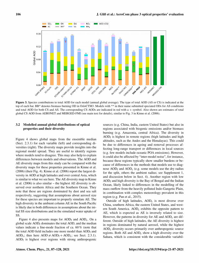
106 J. Gliß et al.: AeroCom phase 3 optical properties’ evaluation
Figure 3. Species contributions to total AOD for each model (annual global average). The type of total AOD (AS or CS) is indicated at thetop of each bar. BB* denotes biomass burning OD in OsloCTM3. Models with ** in their name submitted speciated ODs for AS conditionsand total AOD for both CS and AS. The corresponding CS AODs are indicated in red with a + symbol. Also shown are estimates of totalglobal CS AOD from AERONET and MERGED-FMI (see main text for details), similar to Fig. 3 in Kinne et al. (2006).
3.2 Modelled annual global distributions of opticalproperties and their diversity
Figure 4 shows global maps from the ensemble median(Sect. 2.3.1) for each variable (left) and corresponding di-versities (right). The diversity maps provide insights into theregional model spread. They are useful to identify regionswhere models tend to disagree. This may also help to explaindifferences between models and observations. The AOD andAE diversity maps from this study can be compared with thediversity maps for these properties presented in Kinne et al.(2006) (their Fig. 4). Kinne et al. (2006) report the largest di-versity in AOD at high latitudes and over central Asia, whichis similar to what we see here. The AE diversity map in Kinneet al. (2006) is also similar – the highest AE diversity is ob-served over northern Africa and the Southern Ocean. Theynote that these are regions dominated by dust and sea saltrespectively, suggesting that assumptions about aerosol sizefor these species are important to properly simulate AE. Thehigh diversity in the ambient column AE in the South Pacificis likely due to both differences in assumptions about the ini-tial SS size distributions and in the simulated water uptake ofSS.
Figure 4 also presents maps for AODf and AODc. On aglobal scale AODf dominates the total AOD, and the medianvalues indicate a fine-mode fraction of ca. 60 % (note thatthe total AOD field includes one more model than AODf andAODc; thus here AOD 6=AODf+AODc; see Sect. 2.3.1).AODf is highest over regions with strong anthropogenic
sources (e.g. China, India, eastern United States) but also inregions associated with biogenic emissions and/or biomassburning (e.g. Amazonia, central Africa). The diversity inAODf is highest in remote regions (high latitudes and highaltitudes, such as the Andes and the Himalayas). This couldbe due to differences in ageing and removal processes af-fecting long-range transport or differences in local sources(e.g. few models include oceanic POA emissions). However,it could also be affected by “inter-model noise”, for instance,because these regions typically show smaller burdens or be-cause of differences in the methods that models use to diag-nose AODf and AODc (e.g. some models use the dry radiusfor the split, others the ambient radius; see Supplement 1,and discussion below in Sect. 4). Another region with lowAODf and high diversity is the Bay of Bengal and the IndianOcean, likely linked to differences in the modelling of themass outflow from the heavily polluted Indo-Gangetic Plain,in combination with complex meteorology prevalent in thisregion (e.g. Pan et al., 2015).
Outside of high latitudes, AODc is most diverse overChina, southern Africa, the eastern United States, and west-ern South America. AODc exhibits the opposite pattern toAE, which is expected as AE is inversely related to size.However, the patterns in diversity for AE and AODc are dif-ferent. Outside of high latitudes, the AE diversity is highestin regions dominated by natural aerosol, while the highestAODc diversity occurs primarily over anthropogenic sourceregions. Both AE and AODc show a high diversity over theSahara, which is consistent with the considerable variabil-
Atmos. Chem. Phys., 21, 87–128, 2021 https://doi.org/10.5194/acp-21-87-2021
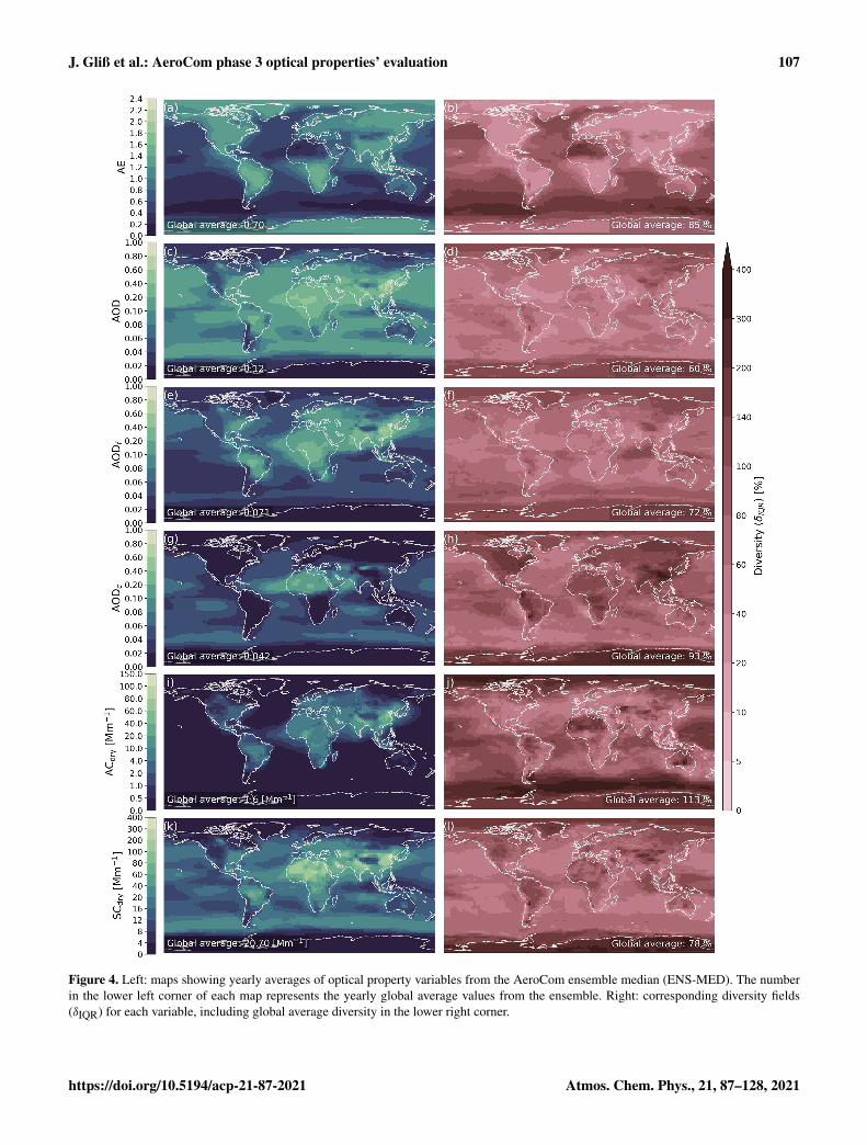
J. Gliß et al.: AeroCom phase 3 optical properties’ evaluation 107
Figure 4. Left: maps showing yearly averages of optical property variables from the AeroCom ensemble median (ENS-MED). The numberin the lower left corner of each map represents the yearly global average values from the ensemble. Right: corresponding diversity fields(δIQR) for each variable, including global average diversity in the lower right corner.
https://doi.org/10.5194/acp-21-87-2021 Atmos. Chem. Phys., 21, 87–128, 2021
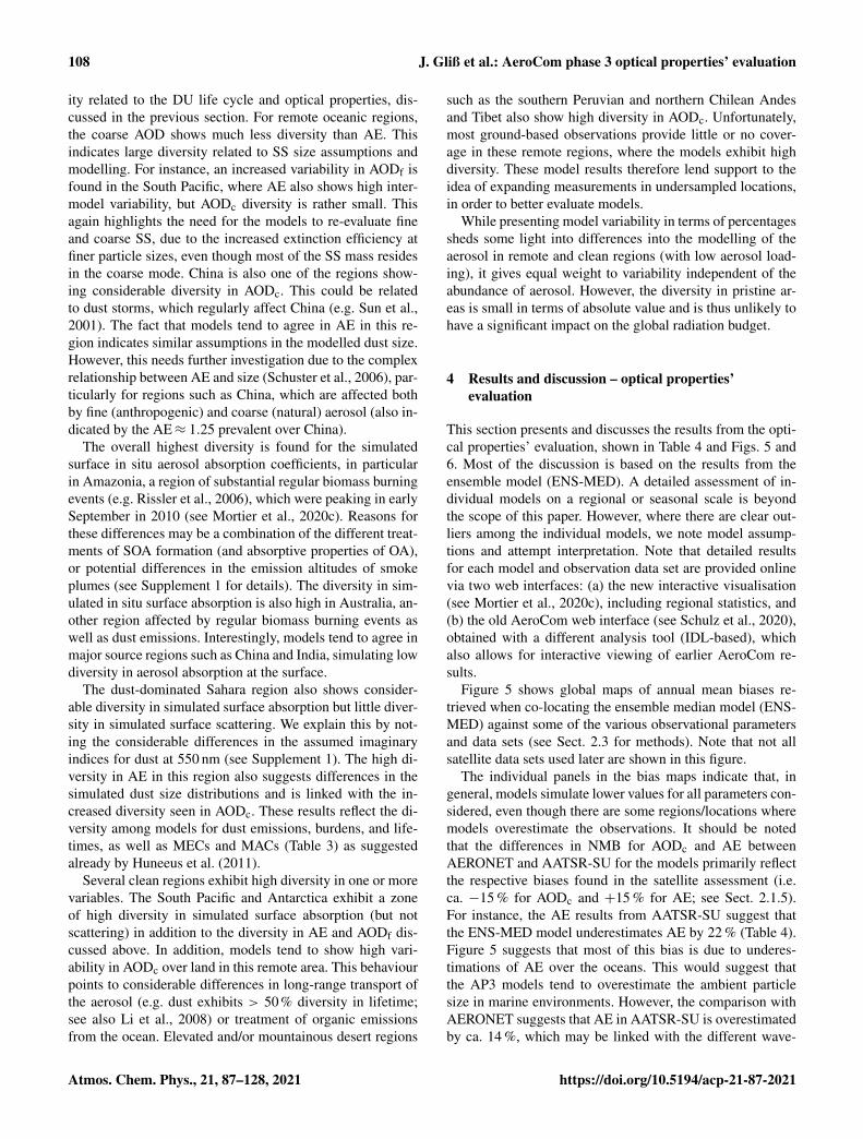
108 J. Gliß et al.: AeroCom phase 3 optical properties’ evaluation
ity related to the DU life cycle and optical properties, dis-cussed in the previous section. For remote oceanic regions,the coarse AOD shows much less diversity than AE. Thisindicates large diversity related to SS size assumptions andmodelling. For instance, an increased variability in AODf isfound in the South Pacific, where AE also shows high inter-model variability, but AODc diversity is rather small. Thisagain highlights the need for the models to re-evaluate fineand coarse SS, due to the increased extinction efficiency atfiner particle sizes, even though most of the SS mass residesin the coarse mode. China is also one of the regions show-ing considerable diversity in AODc. This could be relatedto dust storms, which regularly affect China (e.g. Sun et al.,2001). The fact that models tend to agree in AE in this re-gion indicates similar assumptions in the modelled dust size.However, this needs further investigation due to the complexrelationship between AE and size (Schuster et al., 2006), par-ticularly for regions such as China, which are affected bothby fine (anthropogenic) and coarse (natural) aerosol (also in-dicated by the AE≈ 1.25 prevalent over China).
The overall highest diversity is found for the simulatedsurface in situ aerosol absorption coefficients, in particularin Amazonia, a region of substantial regular biomass burningevents (e.g. Rissler et al., 2006), which were peaking in earlySeptember in 2010 (see Mortier et al., 2020c). Reasons forthese differences may be a combination of the different treat-ments of SOA formation (and absorptive properties of OA),or potential differences in the emission altitudes of smokeplumes (see Supplement 1 for details). The diversity in sim-ulated in situ surface absorption is also high in Australia, an-other region affected by regular biomass burning events aswell as dust emissions. Interestingly, models tend to agree inmajor source regions such as China and India, simulating lowdiversity in aerosol absorption at the surface.
The dust-dominated Sahara region also shows consider-able diversity in simulated surface absorption but little diver-sity in simulated surface scattering. We explain this by not-ing the considerable differences in the assumed imaginaryindices for dust at 550 nm (see Supplement 1). The high di-versity in AE in this region also suggests differences in thesimulated dust size distributions and is linked with the in-creased diversity seen in AODc. These results reflect the di-versity among models for dust emissions, burdens, and life-times, as well as MECs and MACs (Table 3) as suggestedalready by Huneeus et al. (2011).
Several clean regions exhibit high diversity in one or morevariables. The South Pacific and Antarctica exhibit a zoneof high diversity in simulated surface absorption (but notscattering) in addition to the diversity in AE and AODf dis-cussed above. In addition, models tend to show high vari-ability in AODc over land in this remote area. This behaviourpoints to considerable differences in long-range transport ofthe aerosol (e.g. dust exhibits > 50% diversity in lifetime;see also Li et al., 2008) or treatment of organic emissionsfrom the ocean. Elevated and/or mountainous desert regions
such as the southern Peruvian and northern Chilean Andesand Tibet also show high diversity in AODc. Unfortunately,most ground-based observations provide little or no cover-age in these remote regions, where the models exhibit highdiversity. These model results therefore lend support to theidea of expanding measurements in undersampled locations,in order to better evaluate models.
While presenting model variability in terms of percentagessheds some light into differences into the modelling of theaerosol in remote and clean regions (with low aerosol load-ing), it gives equal weight to variability independent of theabundance of aerosol. However, the diversity in pristine ar-eas is small in terms of absolute value and is thus unlikely tohave a significant impact on the global radiation budget.
4 Results and discussion – optical properties’evaluation
This section presents and discusses the results from the opti-cal properties’ evaluation, shown in Table 4 and Figs. 5 and6. Most of the discussion is based on the results from theensemble model (ENS-MED). A detailed assessment of in-dividual models on a regional or seasonal scale is beyondthe scope of this paper. However, where there are clear out-liers among the individual models, we note model assump-tions and attempt interpretation. Note that detailed resultsfor each model and observation data set are provided onlinevia two web interfaces: (a) the new interactive visualisation(see Mortier et al., 2020c), including regional statistics, and(b) the old AeroCom web interface (see Schulz et al., 2020),obtained with a different analysis tool (IDL-based), whichalso allows for interactive viewing of earlier AeroCom re-sults.
Figure 5 shows global maps of annual mean biases re-trieved when co-locating the ensemble median model (ENS-MED) against some of the various observational parametersand data sets (see Sect. 2.3 for methods). Note that not allsatellite data sets used later are shown in this figure.
The individual panels in the bias maps indicate that, ingeneral, models simulate lower values for all parameters con-sidered, even though there are some regions/locations wheremodels overestimate the observations. It should be notedthat the differences in NMB for AODc and AE betweenAERONET and AATSR-SU for the models primarily reflectthe respective biases found in the satellite assessment (i.e.ca. −15 % for AODc and +15 % for AE; see Sect. 2.1.5).For instance, the AE results from AATSR-SU suggest thatthe ENS-MED model underestimates AE by 22 % (Table 4).Figure 5 suggests that most of this bias is due to underes-timations of AE over the oceans. This would suggest thatthe AP3 models tend to overestimate the ambient particlesize in marine environments. However, the comparison withAERONET suggests that AE in AATSR-SU is overestimatedby ca. 14 %, which may be linked with the different wave-
Atmos. Chem. Phys., 21, 87–128, 2021 https://doi.org/10.5194/acp-21-87-2021
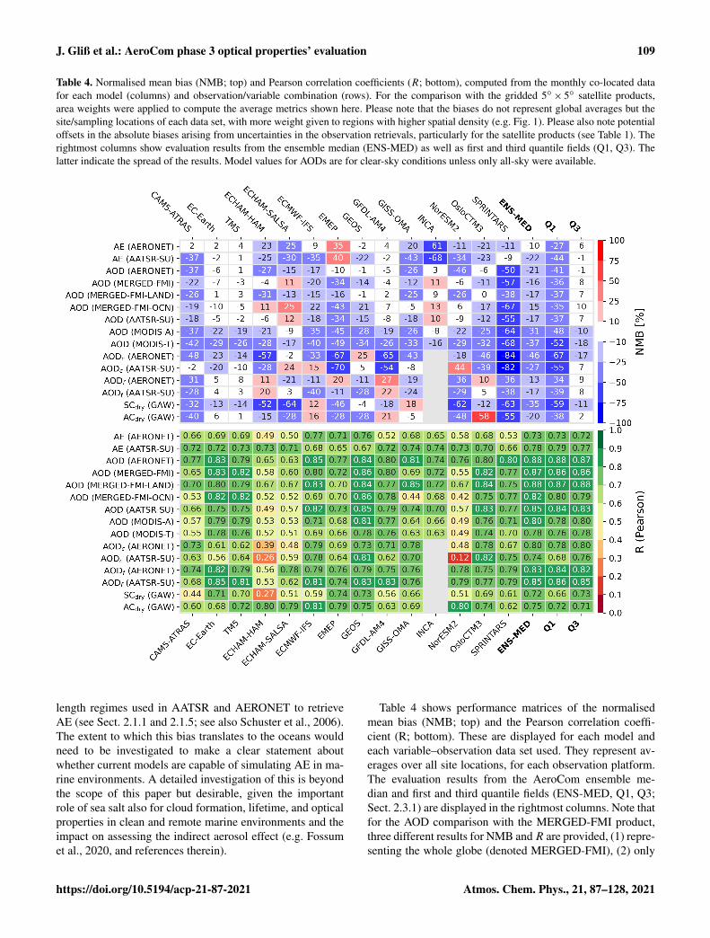
J. Gliß et al.: AeroCom phase 3 optical properties’ evaluation 109
Table 4. Normalised mean bias (NMB; top) and Pearson correlation coefficients (R; bottom), computed from the monthly co-located datafor each model (columns) and observation/variable combination (rows). For the comparison with the gridded 5◦× 5◦ satellite products,area weights were applied to compute the average metrics shown here. Please note that the biases do not represent global averages but thesite/sampling locations of each data set, with more weight given to regions with higher spatial density (e.g. Fig. 1). Please also note potentialoffsets in the absolute biases arising from uncertainties in the observation retrievals, particularly for the satellite products (see Table 1). Therightmost columns show evaluation results from the ensemble median (ENS-MED) as well as first and third quantile fields (Q1, Q3). Thelatter indicate the spread of the results. Model values for AODs are for clear-sky conditions unless only all-sky were available.
length regimes used in AATSR and AERONET to retrieveAE (see Sect. 2.1.1 and 2.1.5; see also Schuster et al., 2006).The extent to which this bias translates to the oceans wouldneed to be investigated to make a clear statement aboutwhether current models are capable of simulating AE in ma-rine environments. A detailed investigation of this is beyondthe scope of this paper but desirable, given the importantrole of sea salt also for cloud formation, lifetime, and opticalproperties in clean and remote marine environments and theimpact on assessing the indirect aerosol effect (e.g. Fossumet al., 2020, and references therein).
Table 4 shows performance matrices of the normalisedmean bias (NMB; top) and the Pearson correlation coeffi-cient (R; bottom). These are displayed for each model andeach variable–observation data set used. They represent av-erages over all site locations, for each observation platform.The evaluation results from the AeroCom ensemble me-dian and first and third quantile fields (ENS-MED, Q1, Q3;Sect. 2.3.1) are displayed in the rightmost columns. Note thatfor the AOD comparison with the MERGED-FMI product,three different results for NMB andR are provided, (1) repre-senting the whole globe (denoted MERGED-FMI), (2) only
https://doi.org/10.5194/acp-21-87-2021 Atmos. Chem. Phys., 21, 87–128, 2021
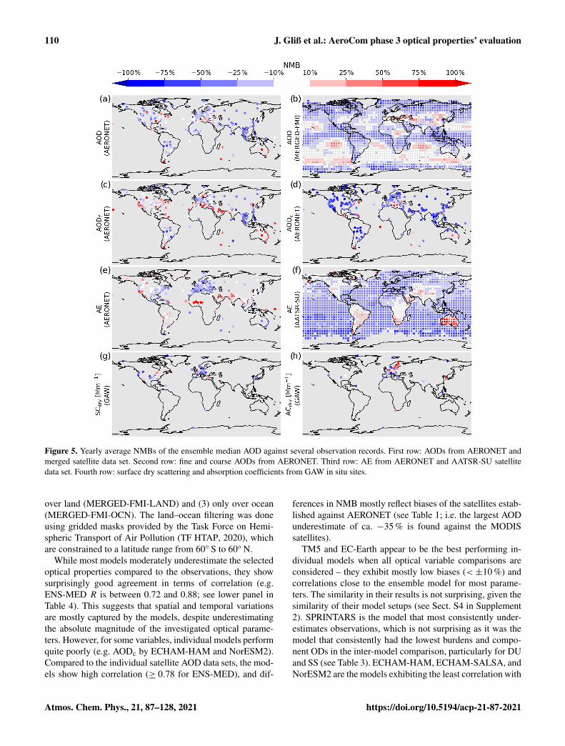
110 J. Gliß et al.: AeroCom phase 3 optical properties’ evaluation
Figure 5. Yearly average NMBs of the ensemble median AOD against several observation records. First row: AODs from AERONET andmerged satellite data set. Second row: fine and coarse AODs from AERONET. Third row: AE from AERONET and AATSR-SU satellitedata set. Fourth row: surface dry scattering and absorption coefficients from GAW in situ sites.
over land (MERGED-FMI-LAND) and (3) only over ocean(MERGED-FMI-OCN). The land–ocean filtering was doneusing gridded masks provided by the Task Force on Hemi-spheric Transport of Air Pollution (TF HTAP, 2020), whichare constrained to a latitude range from 60◦ S to 60◦ N.
While most models moderately underestimate the selectedoptical properties compared to the observations, they showsurprisingly good agreement in terms of correlation (e.g.ENS-MED R is between 0.72 and 0.88; see lower panel inTable 4). This suggests that spatial and temporal variationsare mostly captured by the models, despite underestimatingthe absolute magnitude of the investigated optical parame-ters. However, for some variables, individual models performquite poorly (e.g. AODc by ECHAM-HAM and NorESM2).Compared to the individual satellite AOD data sets, the mod-els show high correlation (≥ 0.78 for ENS-MED), and dif-
ferences in NMB mostly reflect biases of the satellites estab-lished against AERONET (see Table 1; i.e. the largest AODunderestimate of ca. −35 % is found against the MODISsatellites).
TM5 and EC-Earth appear to be the best performing in-dividual models when all optical variable comparisons areconsidered – they exhibit mostly low biases (<±10 %) andcorrelations close to the ensemble model for most parame-ters. The similarity in their results is not surprising, given thesimilarity of their model setups (see Sect. S4 in Supplement2). SPRINTARS is the model that most consistently under-estimates observations, which is not surprising as it was themodel that consistently had the lowest burdens and compo-nent ODs in the inter-model comparison, particularly for DUand SS (see Table 3). ECHAM-HAM, ECHAM-SALSA, andNorESM2 are the models exhibiting the least correlation with
Atmos. Chem. Phys., 21, 87–128, 2021 https://doi.org/10.5194/acp-21-87-2021
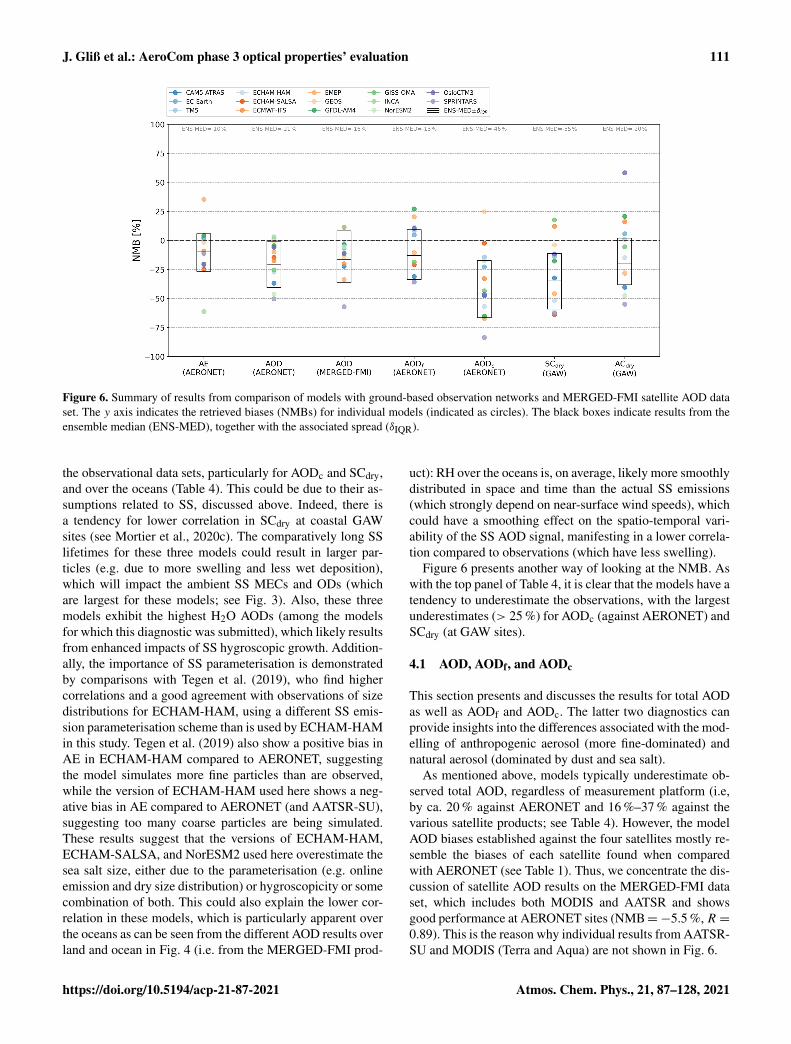
J. Gliß et al.: AeroCom phase 3 optical properties’ evaluation 111
Figure 6. Summary of results from comparison of models with ground-based observation networks and MERGED-FMI satellite AOD dataset. The y axis indicates the retrieved biases (NMBs) for individual models (indicated as circles). The black boxes indicate results from theensemble median (ENS-MED), together with the associated spread (δIQR).
the observational data sets, particularly for AODc and SCdry,and over the oceans (Table 4). This could be due to their as-sumptions related to SS, discussed above. Indeed, there isa tendency for lower correlation in SCdry at coastal GAWsites (see Mortier et al., 2020c). The comparatively long SSlifetimes for these three models could result in larger par-ticles (e.g. due to more swelling and less wet deposition),which will impact the ambient SS MECs and ODs (whichare largest for these models; see Fig. 3). Also, these threemodels exhibit the highest H2O AODs (among the modelsfor which this diagnostic was submitted), which likely resultsfrom enhanced impacts of SS hygroscopic growth. Addition-ally, the importance of SS parameterisation is demonstratedby comparisons with Tegen et al. (2019), who find highercorrelations and a good agreement with observations of sizedistributions for ECHAM-HAM, using a different SS emis-sion parameterisation scheme than is used by ECHAM-HAMin this study. Tegen et al. (2019) also show a positive bias inAE in ECHAM-HAM compared to AERONET, suggestingthe model simulates more fine particles than are observed,while the version of ECHAM-HAM used here shows a neg-ative bias in AE compared to AERONET (and AATSR-SU),suggesting too many coarse particles are being simulated.These results suggest that the versions of ECHAM-HAM,ECHAM-SALSA, and NorESM2 used here overestimate thesea salt size, either due to the parameterisation (e.g. onlineemission and dry size distribution) or hygroscopicity or somecombination of both. This could also explain the lower cor-relation in these models, which is particularly apparent overthe oceans as can be seen from the different AOD results overland and ocean in Fig. 4 (i.e. from the MERGED-FMI prod-
uct): RH over the oceans is, on average, likely more smoothlydistributed in space and time than the actual SS emissions(which strongly depend on near-surface wind speeds), whichcould have a smoothing effect on the spatio-temporal vari-ability of the SS AOD signal, manifesting in a lower correla-tion compared to observations (which have less swelling).
Figure 6 presents another way of looking at the NMB. Aswith the top panel of Table 4, it is clear that the models have atendency to underestimate the observations, with the largestunderestimates (> 25 %) for AODc (against AERONET) andSCdry (at GAW sites).
4.1 AOD, AODf, and AODc
This section presents and discusses the results for total AODas well as AODf and AODc. The latter two diagnostics canprovide insights into the differences associated with the mod-elling of anthropogenic aerosol (more fine-dominated) andnatural aerosol (dominated by dust and sea salt).
As mentioned above, models typically underestimate ob-served total AOD, regardless of measurement platform (i.e,by ca. 20 % against AERONET and 16 %–37 % against thevarious satellite products; see Table 4). However, the modelAOD biases established against the four satellites mostly re-semble the biases of each satellite found when comparedwith AERONET (see Table 1). Thus, we concentrate the dis-cussion of satellite AOD results on the MERGED-FMI dataset, which includes both MODIS and AATSR and showsgood performance at AERONET sites (NMB=−5.5 %,R =0.89). This is the reason why individual results from AATSR-SU and MODIS (Terra and Aqua) are not shown in Fig. 6.
https://doi.org/10.5194/acp-21-87-2021 Atmos. Chem. Phys., 21, 87–128, 2021
112 J. Gliß et al.: AeroCom phase 3 optical properties’ evaluation
The consistent AOD underestimate in the models meansthat they are either simulating too little mass loading in thecolumn and/or underestimating the column optical extinc-tion efficiency (e.g. related to assumptions about size, MEC,and/or composition). Figure 6 suggests that most of the AODbias is due to missing (or optically too inefficient) coarseaerosol, which also exhibits the largest diversity (in termsof bias) among the models and shows lower correlation thanAOD and AODf (Table 4). However, as pointed out above,about half of the models computed AODf using the dry par-ticle radius (see also Supplement 1). These models likely at-tribute some extinction to the fine mode that should be at-tributed to AODc if hygroscopic swelling was accounted for.
The impact of this uncertainty was investigated using7 models that submitted diagnostics of fine and total SSOD. Four of these, CAM5-ATRAS, GEOS, GISS-OMA, andSPRINTARS, computed AODf based on the dry radius, whilethe other three, EC-Earth, TM5, and ECMWF-IFS, used theambient particle radius. The first four models suggest a SSfine-mode fraction of ca. 26 %, while the latter three modelssuggest 15 %. Thus, ca. 11 % of the SS OD is erroneously at-tributed to AODf when the dry radius is used to split fine andcoarse mode. On a global scale, ca. 33 % of the total AODis due to SS (Table 3). Hence, ca. 3 % too much of the totalAOD is attributed to AODf if the dry radius is used, assumingthat SS is the dominant species affected by this error. This isa fair assumption as other hydrophilic species typically re-side in the accumulation mode, and dust is assumed to behydrophobic in most models.
Thus, for the affected models, AODc is likely slightlyshifted towards less negative biases by ca. 3 %, while AODfwould show larger underestimations, accordingly. The diver-sity in AODc could be in parts due to the different methodolo-gies used in the models to determine the size threshold; how-ever, this is not the sole explanation, since the AODf exhibitsless diversity. Also, the diversity in AODc is consistent withthe large diversity found for dust and sea salt aerosol amongthe models (see Sect. 3) and highlights the large uncertain-ties associated with the modelling of these natural aerosols(see Sect. 3). Attempts to address these uncertainties are alsoreflected in the substantial changes in AP3 compared to AP1(e.g. less and optically more inefficient dust and more sea saltin AP3). Figure 5b does not allow a clear statement relatedto over- or underestimates of dust and sea salt. For instance,in several remote ocean regions ENS-MED exhibits positivebiases (e.g. South Pacific), whereas in other regions slightlynegative biases or good agreement are found. This suggeststhat, overall, models manage to capture the overall magni-tude of the sea salt contribution. Most of the coarse AOD biasseems to be associated with continental land masses (e.g. SEAsia, Arabian Peninsula; Fig. 5d), which is also indicatedby the lower underestimate when comparing AODc againstAATSR, instead of AERONET (Table 4).
We stress that the fact that models tend to match themagnitude of the AOD in sea-salt-dominated regions does
not necessarily reflect that the processes leading to theseAODs are represented correctly. In this context we refer oncemore to the large diversity (and compensating effects) asso-ciated with SS emissions (computed online), burdens, life-time, and MECs and the substantial changes since AP1 (seeSect. 3 for details). This is further supported by the typicallydecreased correlations found when comparing models withsatellite data sets (which “see” both oceans and continentalland masses; see, for example, results from MERGED-FMI,LAND versus OCN in Table 4). For instance, ENS-MED ex-hibits comparatively low correlation in the SW and S. Pacificcompared to the satellites (see online results; Mortier et al.,2020c). However, these regions are affected by high cloudcoverage throughout the year, and thus the lower correlationmay also be due to representation errors in the monthly satel-lite aggregates used.
ECHAM-SALSA and INCA are the only models whichslightly overestimate AOD, when compared with two satel-lite products (MERGED-FMI and AATSR). The overesti-mates by ECHAM-SALSA and INCA have some of thelargest contributions of SS and sulfate to AOD (Fig. 3). Bothmodels exhibit overestimates of AOD over the ocean as canbe seen in comparison with MERGED-FMI-OCN (see Ta-ble 4), suggesting an overestimated contribution of sea saltto AOD. In the case of ECHAM-SALSA, this is furtherconfirmed by the overestimated AODc (by ca. 24 %) com-pared to the AATSR data set (in addition, ECHAM-SALSAis one of the models using dry radius to compute AODf,thus likely overestimating the fine-mode fraction diagnosedthrough AODc and AODf). However, note again that AODcfrom AATSR is underestimated by ca. 15 % at AERONETsites (Table 1). Thus, it is difficult to draw clear conclusionsabout the magnitude of the model bias over marine environ-ments.
AOD underestimates are mostly associated with SE Asiaand Amazonia, Siberia, and high latitudes in general (seeFig. 5a, b). The latter may be associated with insufficienttransport towards the poles (e.g. Stohl, 2006) or associatedphenomena affecting the radiative properties of the Arcticatmosphere (such as Arctic haze; e.g. Tunved et al., 2013)– perhaps linked with an insufficient attribution of the exten-sive wildfires in Russia in the summer of 2010 (e.g. Mielonenet al., 2012). The negative bias in S. America (i.e. AERONETAOD∼ 0.5, while ENS-MED∼ 0.3; see web results; Mortieret al., 2020c) mostly arises from an underestimate in thebiomass burning season in 2010. However, compared to theAP1 simulations (which simulated too early a biomass burn-ing season in S. America; Kinne et al., 2006), the AP3 mod-els match the timing of the biomass burning season well(which peaked in August–September in 2010).
Explaining the AOD underestimate in SE Asia is not triv-ial. SE Asia has substantial anthropogenic emissions whichare fairly harmonised among the AP3 models (see Sect. 3).This can also be seen by the comparatively low diversity insurface SCdry and AODf in Fig. 4. The region is also strongly
Atmos. Chem. Phys., 21, 87–128, 2021 https://doi.org/10.5194/acp-21-87-2021
J. Gliß et al.: AeroCom phase 3 optical properties’ evaluation 113
affected by a pronounced seasonality including an intensivebiomass burning season, dust inflow (e.g. transported fromthe Arabian Peninsula), monsoon seasons (i.e. seasonality inwet deposition), and other factors impacting the abundanceand properties of aerosol (e.g. fog and hygroscopicity), mak-ing it difficult for models to simulate regional and seasonalaerosol loadings (e.g. Pan et al., 2015). However, as can beseen in Fig. 5d, most of the AOD bias in this region is due tomissing (or optically too inefficient) coarse particles, whichis also supported by the overestimated AE in that region (e.g.Fig. 5e). Thus, the bias could be related to insufficient dusttransport or dust particles that are too coarse (and opticallyless efficient). This hypothesis is consistent with the gener-ally low burden, MEC, and OD associated with dust in AP3discussed above (Sect. 3). A detailed investigation of the AP3models in this important region is desirable but beyond thescope of this paper, due to the complexity of the prevailingprocesses.
It is also interesting to compare the relative differences inmodel simulations of AOD for the different observation plat-forms. NorESM2, for instance, is the only model that seemsto exhibit a weaker performance (in terms of bias) simulatingAERONET AOD than simulating any of the satellite AODs.The large underestimate over land could be linked with itscomparatively low SO4 and dust optical depths (see Table 3),resulting in substantial AOD underestimates compared toAERONET. The seemingly better performance when com-pared to the satellite products is due to an overestimate ofthe SS contribution (particularly in the Southern Ocean),which compensates to some degree for the underestimateover land (see also Fig. 3). The latter is likely due to theSS size assumptions discussed above, resulting in a shift to-wards finer sea salt aerosol that is optically too efficient. Theoverestimated sea salt optical depth manifests particularly inthe comparison with the AODc data from AATSR (NMB=44 %) and the 6 % overestimate compared to MERGED-FMI-OCN. As discussed above, the lower correlation overthe oceans suggests too much hygroscopic swelling, likelyresulting in a smoothing of the spatio-temporal variability ofmarine aerosol.
In contrast, EMEP and GEOS exhibit larger underesti-mates in AOD when compared with the satellites. In the caseof EMEP, this is likely due to too little SS mass, for the rea-sons discussed above, and it can be seen particularly in theincreased underestimate in AODc. In the case of GEOS, thelarger AOD underestimate against the satellites could be dueto sea salt particles that are too coarse and optically too inef-ficient (comparatively low SS MEC; see Table 3), in agree-ment with Bian et al. (2019).
In contrast to the large underestimate of AODc, modelstend to agree better in the AODf, showing less underesti-mation and higher correlation (Table 4). To some degree,this may be linked with more harmonised emissions of theassociated anthropogenic aerosol species. However, as wasshown in Sect. 3, models also show considerable diversity
in fine aerosol species (e.g. OA, SO4; see Fig. 2), a resultof differences associated with secondary formation but alsodue to differences in MEC. Hence, it is interesting to seethat models tend to agree better in AODf when comparedwith observations. In addition, the associated particle sizes inthe accumulation mode are optically more efficient. There-fore, the AODf may be influenced also by dust or sea salt,dependent on the region – even though their mass primar-ily resides in the coarse regime. For instance, as discussedabove, approximately 15 % of the sea salt OD resides in thefine mode. The dust fine-mode fraction was found to be ca.30 % and was retrieved based on dust fine-mode ODs sub-mitted by the same models used above to estimate the SSfine-mode fraction (i.e. CAM5-ATRAS, GEOS, GISS-OMA,SPRINTARS, EC-Earth, TM5, ECMWF-IFS). Compared toAERONET, ENS-MED overestimates AODf in several re-gions, including the Mediterranean, the United States, Aus-tralia, and the Arabian Peninsula (see Fig. 5c). The lattercould be an indication of dust size distributions that are toofine contributing to the AODf. Overall, these overestimatesof AODf in some regions tend to have a compensating ef-fect on the underestimate in AODc, resulting in a seeminglybetter model performance for total AOD (see Fig. 5). Thiscould be due, in part, to uncertainties related to aerosol size(e.g. too much fine dust, which is optically more efficientand results in an overestimate of AODf, while missing in thecoarse mode). However, it could also be simply due to toomuch fine anthropogenic aerosol such as SO4 and too littlecoarse aerosol. GFDL-AM4, for instance, exhibits consider-able overestimates of AODf compared to both AERONETand AATSR while strongly underestimating AODc, result-ing in quite good an agreement in total AOD. All three pa-rameters (AOD, AODf, and AODc) exhibit high correlation.Compared to the ensemble median, this model shows above-average MECs and ODs for both OA and SO4, which couldexplain the overestimated AODf. DU and SS, on the con-trary, are close to the ensemble median, which would ex-plain the underestimate of AODc. Other models that over-estimate AODf include ECHAM-HAM, OsloCTM3 (bothagainst AERONET and AATSR), and EMEP (only againstAERONET). It is difficult to identify a common character-istic amongst these models that might explain the overesti-mate, but in the case of ECHAM-HAM and OsloCTM3 itmay be due to comparatively large sulfate burdens and ODswhich could be linked with above-average DMS emissions(not shown). For EMEP, on the other hand, it is more likelydue to its relatively large contributions from OA, NO3, andNH4 (see Fig. 3), since SO4 appears to be underrepresented(see Table 3). Another possible reason for EMEP’s over-estimation of AODf is that fine sea salt and dust particlesare assumed to have diameters smaller than 2.5 µm, so thatthe extinction due to sea salt and dust aerosols with diame-ters between 1–2.5 µm contributes to the (overestimated) finemode rather than the (underestimated) coarse mode. Theseresults suggest a complex interplay among various model
https://doi.org/10.5194/acp-21-87-2021 Atmos. Chem. Phys., 21, 87–128, 2021
114 J. Gliß et al.: AeroCom phase 3 optical properties’ evaluation
assumptions related to composition and size. Mortier et al.(2020b) also find poorer model performances (larger biasesand higher inter-model variability) in long-term trends ofthe AODc, as compared to measurements of total AOD andAODf.
4.2 Column Ångström exponent (AE)
Models are fairly consistent in their underestimate of AE(see Table 4). This suggests that they are (1) either simulat-ing larger particles than are observed or (2) underestimatingthe fine-mode fraction. EMEP shows the largest overestimatein AE, both compared to AERONET and AATSR-SU. Thisis likely related to the lower MEC and burden for SS andDU relative to the ensemble model (Table 3) and the cut-offfor fine SS and DU at 2.5 µm. INCA, in contrast, exhibitsthe largest underestimate of AE for both AERONET andAATSR-SU, which is likely linked with the comparativelylong dust and sea salt lifetimes and the corresponding highburdens (Table 3). The two ECHAM models exhibit similarspecies optical depths to those simulated by INCA (Fig. 3),so other factors (e.g. assumptions about coarse-mode sizedistributions) may also play a role.
As discussed above, the comparison with AATSR-SU(Fig. 5f) suggests that models underestimate AE over theoceans; however, there is a large uncertainty due to difficul-ties in validating satellite products over the oceans. In thiscontext, the apparent large overestimate of AE over Aus-tralia compared to AATSR (Fig. 5f) is likely associated withretrieval errors in the satellite product. The few AERONETsites in Australia suggest that ENS-MED underestimates AE(Fig. 5e).
Figure 5e shows that models tend to overestimate AE industy regions (e.g. Sahara, Arabian Peninsula), suggestingthat they tend to simulate dust particles that are too small. Inthe case of the Arabian Peninsula, this is consistent with theoverestimated AODf and the underestimated AODc (Fig. 5c,d).
However, several regions exhibit a larger underestimatein AODc than AODf in ENS-MED while also underesti-mating AE (e.g. Europe). As can be seen in Table 4, fiveout of the 14 models (ECHAM-HAM, ECMWF-IFS, GISS-OMA, OsloCTM3, SPRINTARS) show such apparent in-consistencies among AE, AODf, and AODc in comparisonwith AERONET. To some degree, these seemingly inconsis-tent results for these three parameters may be affected byuncertainties related to the separation of AODf and AODcboth in the models (as discussed above) and the observa-tions (as discussed for AERONET in Sect. 2.1.1). GISS-OMA, OsloCTM3, and SPRINTARS are among the modelswhich use the dry particle radius to split AOD into AODfand AODc. In addition, OsloCTM3 simulates dust and seasalt in eight size bins, and one of these bins contributes bothto the R < 0.5 µm and R > 0.5 µm regime but is accountedfor in the AODf diagnostic computed for AeroCom. In the
case of ENS-MED, the results may be affected by the av-eraging choices related to AE and AODf (see Sect. 2.3.1).However, even though these uncertainties are not negligible,they cannot explain the large differences observed in the bi-ases. ECHAM-HAM, for instance, shows an AE underesti-mation of 23 % compared to AERONET while at the sametime overestimating AODf by ca. 11 % and underestimatingAODc by ca. 57 %.
This analysis clearly shows the difficulty of interpretingmodel AE biases averaged over whole regions and on an an-nual basis. As Schuster et al. (2006) point out, the relation-ship between AE and the aerosol size distribution is com-plex and allows for only qualitative statements. Here, wefound that models tend to underestimate the global medianAE, which suggests that overall they tend to simulate an ex-cess of fine particles or relatively too little coarse aerosol. Inorder to investigate this in more detail, an additional sensi-tivity study was performed, in which the model biases wereanalysed as a function of the observed AE. The results ofthis study are shown in Fig. 7, where all models were co-located with AERONET AE observations and segregated bydifferent AE intervals. For coarse-mode-dominated aerosolwith AE< 1 (i.e. bins 1 and 2 in Fig. 7), the AP3 mod-els tend to overestimate AE, with INCA being the only ex-ception. For instance, ENS-MED overestimates AE substan-tially (ca.+140 %) if only AE measurements below values of0.5 are considered. On the other hand, for more fine-mode-dominated aerosol (i.e. AE> 2, bins 5 and 6), all models tendto show larger underestimates in AE compared to the generalresults presented above that consider the full range of (non-binned) AE measurements. For instance, ENS-MED showsa bias of ca. −60 % if only AE> 2 measurements are con-sidered. These results suggest that simulated fine-dominatedaerosol is larger than it should be (based on the observations),while coarse-dominated aerosol is smaller than it should be.The latter is consistent with the above observation that AE issubstantially overestimated in dusty regions.
4.3 Dry surface scattering coefficient (SCdry)
This and the following section present and discuss the re-sults from the comparison with surface “dry” (RH< 40 %)in situ measurements at GAW sites (see Fig. 1g, h for sitelocations). Compared to the previously discussed columnarvariables, these comparisons are more sensitive to modellinguncertainties associated with the vertical dimension (such astransport and mixing). On the other hand, these comparisonsof “dry” variables are “closer” to the simulated aerosol, asthey minimise (but do not eliminate) the impact of water up-take on the optical properties.
As with loading through the column, most models also un-derestimate loading at the surface as indicated by the primar-ily blue shading for surface scattering in Table 4. The modelmedian bias is −35 % for dry scattering; however, the in-dividual model results show considerable diversity, similar
Atmos. Chem. Phys., 21, 87–128, 2021 https://doi.org/10.5194/acp-21-87-2021
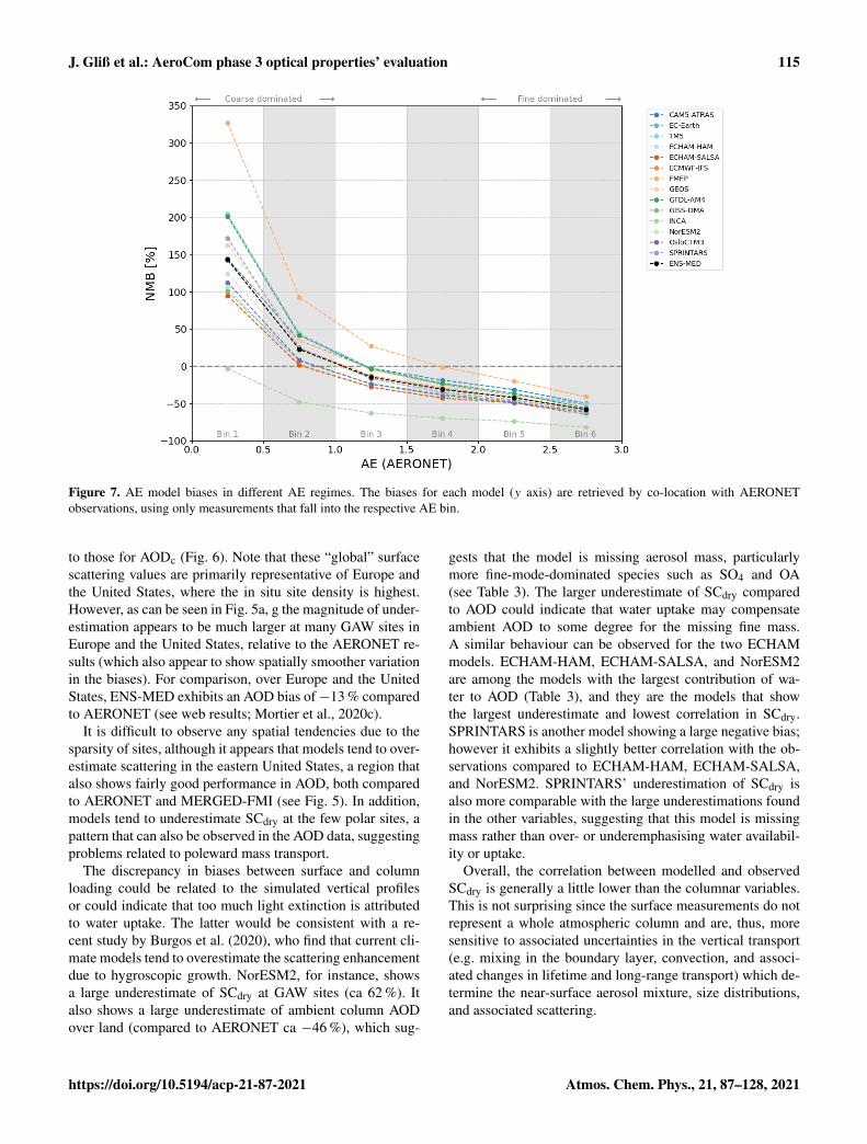
J. Gliß et al.: AeroCom phase 3 optical properties’ evaluation 115
Figure 7. AE model biases in different AE regimes. The biases for each model (y axis) are retrieved by co-location with AERONETobservations, using only measurements that fall into the respective AE bin.
to those for AODc (Fig. 6). Note that these “global” surfacescattering values are primarily representative of Europe andthe United States, where the in situ site density is highest.However, as can be seen in Fig. 5a, g the magnitude of under-estimation appears to be much larger at many GAW sites inEurope and the United States, relative to the AERONET re-sults (which also appear to show spatially smoother variationin the biases). For comparison, over Europe and the UnitedStates, ENS-MED exhibits an AOD bias of−13 % comparedto AERONET (see web results; Mortier et al., 2020c).
It is difficult to observe any spatial tendencies due to thesparsity of sites, although it appears that models tend to over-estimate scattering in the eastern United States, a region thatalso shows fairly good performance in AOD, both comparedto AERONET and MERGED-FMI (see Fig. 5). In addition,models tend to underestimate SCdry at the few polar sites, apattern that can also be observed in the AOD data, suggestingproblems related to poleward mass transport.
The discrepancy in biases between surface and columnloading could be related to the simulated vertical profilesor could indicate that too much light extinction is attributedto water uptake. The latter would be consistent with a re-cent study by Burgos et al. (2020), who find that current cli-mate models tend to overestimate the scattering enhancementdue to hygroscopic growth. NorESM2, for instance, showsa large underestimate of SCdry at GAW sites (ca 62 %). Italso shows a large underestimate of ambient column AODover land (compared to AERONET ca −46 %), which sug-
gests that the model is missing aerosol mass, particularlymore fine-mode-dominated species such as SO4 and OA(see Table 3). The larger underestimate of SCdry comparedto AOD could indicate that water uptake may compensateambient AOD to some degree for the missing fine mass.A similar behaviour can be observed for the two ECHAMmodels. ECHAM-HAM, ECHAM-SALSA, and NorESM2are among the models with the largest contribution of wa-ter to AOD (Table 3), and they are the models that showthe largest underestimate and lowest correlation in SCdry.SPRINTARS is another model showing a large negative bias;however it exhibits a slightly better correlation with the ob-servations compared to ECHAM-HAM, ECHAM-SALSA,and NorESM2. SPRINTARS’ underestimation of SCdry isalso more comparable with the large underestimations foundin the other variables, suggesting that this model is missingmass rather than over- or underemphasising water availabil-ity or uptake.
Overall, the correlation between modelled and observedSCdry is generally a little lower than the columnar variables.This is not surprising since the surface measurements do notrepresent a whole atmospheric column and are, thus, moresensitive to associated uncertainties in the vertical transport(e.g. mixing in the boundary layer, convection, and associ-ated changes in lifetime and long-range transport) which de-termine the near-surface aerosol mixture, size distributions,and associated scattering.
https://doi.org/10.5194/acp-21-87-2021 Atmos. Chem. Phys., 21, 87–128, 2021
116 J. Gliß et al.: AeroCom phase 3 optical properties’ evaluation
ECMWF-IFS and GISS-OMA are the only two mod-els that show a slight overestimation of SCdry (12 % and18 %, respectively), and both exhibit fairly good correlation(R ∼ 0.60). Based on the other results for these models (seeTables 3 and 4), no clear explanations can be provided forthese results, and it would require more detailed investiga-tions of the temporal and spatial distributions (particularlyin the vertical), predominant aerosol types and mixtures, andthe resulting size distributions.
Issues with simulated aerosol size likely also play a rolein the ability of models to simulate surface scattering. Spec-tral scattering measurements are available for most surfacesites, so AE for the surface scattering measurements couldbe compared with model simulations of AE. Many sites alsomeasure surface scattering at two size cuts (PM1 and PM10;Andrews et al., 2019), which could provide a further con-straint on the aerosol size evaluation.
However, note again that this intercomparison bears someuncertainties; for instance, the model data correspond toRH= 0 %, while the measurements correspond to RH<40 %, which is typically considered “dry”. Measurements byZieger et al. (2013) suggest that hygroscopic growth at lowRH could lead to an enhancement in scattering of up to 20 %for the so-called “dry” aerosol measured at RH= 40 %. Onaverage, the measurements considered here were performedat ∼ 24 % RH; thus the impact of light scattering enhance-ment in the observations should be well below 20 % (al-though that will be site-/season-specific).
Another uncertainty is the use of a climatology utilisingdata available between 2005–2015. Comparison with clima-tological values was done to increase the number of sites con-sidered as many sites began measuring after 2010 (see Fig. 3in Laj et al., 2020). However, we investigated the differencesand found that SCdry is larger for most models when compar-ing them with only 2010 surface measurements (not shown).For instance, ENS-MED shows an underestimation of−42 %when compared to 2010 observations, as opposed to −35 %when compared to the 2005–2015 climatology as was donehere. The same comparison was done for ACdry, indicat-ing minimal differences in the ACdry bias (ENS-MED biasof −21.3 % for 2010 and −20.3 % using the climatology).The 2010 results are also available online and can be com-pared with the climatology-based results (see EBAS-CLIM,EBAS-2010 in Mortier et al., 2020c). One factor that likelyimpacts the climatological results is that (1) the site densityincreased in more recent years (e.g. Laj et al., 2020), par-ticularly in Europe and the United States, and (2) these re-gions are associated with negative trends in scattering andabsorption (Collaud Coen et al., 2020; Mortier et al., 2020b).This could shift the weight in the climatology to more re-cent measurements or to regions affected by larger changesbetween 2005–2015. While it would be useful to further ex-plore the impact of climatology versus exact temporal match-ing, such effort is beyond the scope of this paper. Fortunately,our choice of using the surface data climatology for model
evaluation does not appear to impact our results substantially,primarily because of the large differences among the modelsand their tendency to underestimate these variables substan-tially (see Table 4).
4.4 Dry surface absorption coefficient (ACdry)
Models tend to underestimate the surface aerosol absorp-tion coefficients. The results of ENS-MED suggest an aver-age underestimation of ca. 20 %. Interestingly, compared toSCdry, the ACdry observations are better correlated with themodel simulations (R ∼ 0.75) and also less underestimated.This could be linked with the fact that ACdry depends less onhygroscopic growth and that absorption is mostly associatedwith a single species (BC), which reduces impacts of mixingon size distributions and optical properties. This is particu-larly the case for anthropogenic source regions like Europeand the United States, which is consistent with the low inter-model diversity in ACdry in Europe and the United States,compared to SCdry (see Fig. 4j, l). Note, however, that theACdry results primarily represent Europe (and less the UnitedStates compared to SCdry) as can be seen in Fig. 5g and h.
At the few Arctic sites, models tend to significantly un-derestimate ACdry (apart from Utqiagvik (formerly Barrow),where good agreement is found), as suggested by the ENS-MED results shown in Fig. 5g and h. This could be dueto insufficient mass transport into the Arctic or could alsobe linked with Arctic wintertime phenomena resulting inincreased domestic BC and OC emissions, combined withtrapped air masses due to typically strong winter time inver-sions, with substantial impacts on Arctic climate change (see,for example, Sand et al., 2013, and references therein). TheRussian wildfires in 2010 (e.g. Mielonen et al., 2012) mayalso have played a role in this. Another pattern is an appar-ent overestimate of ACdry at the few northern Scandinaviansites, as opposed to the underestimations in most of Europe.Whether this behaviour is linked with 2010 wildfires and/orinsufficient transport and local emissions should be investi-gated in more detail. Two sites in Asia (both on the KoreanPeninsula) also show overestimated ACdry while exhibitingunderestimated SCdry (see Fig. 5g). Reasons for that shouldbe examined in detail but may be linked with overestimatedimpacts of local anthropogenic emissions and/or transport.The same applies for the Cape Point site in South Africa.
With a bias of −55 %, SPRINTARS exhibits the largestunderestimate of ACdry. This is consistent with the resultsfound for all other extensive variables investigated for thismodel. SPRINTARS also exhibits the lowest BC MAC value(which was also the case in AP1; see Koch et al., 2009).This would most certainly contribute to the underestimatein ACdry as the BC burden for SPRINTARS is comparableto that for the other models. This further suggests that theassumptions describing the conversion from BC mass to ab-sorption may play a role and are likely linked with the simu-lated size distributions (which depend on ageing and mixing)
Atmos. Chem. Phys., 21, 87–128, 2021 https://doi.org/10.5194/acp-21-87-2021

J. Gliß et al.: AeroCom phase 3 optical properties’ evaluation 117
and with the lifetime of BC. Unfortunately, SPRINTARS didnot provide the diagnostics to derive BC lifetime. However,as all other species show below-average lifetimes in SPRINT-ARS, it is not unlikely that BC does so too. In summary, theshort lifetimes and large underestimations in loading point toremoval processes in SPRINTARS that are too efficient.
Five models overestimate surface absorption (EC-Earth,TM5, ECMWF-IFS, GFDL-AM4, and OsloCTM3). With abias of +58 %, OsloCTM3 shows the largest overestimateof ACdry. This is related to the implementation of new ab-sorption parameterisations in the model, resulting in a fairlyhigh BC MAC of 13 m2/g, in combination with a strong ver-tical gradient of BC (and OA) in the lower atmosphere (notshown). The considerable difference in OsloCTM3’s abil-ity to simulate ACdry (overestimated) and SCdry (underes-timated) is likely linked with the fact that SO4, one of themain contributors to scattering, does not show such a strongvertical gradient (Gunnar Myhre, personal communication,2020).
As with ECMWF-IFS’s overestimate of SCdry, no clearexplanation can be provided for the positive bias in near-surface ACdry for this model. However, the fact that bothvariables are overestimated in this model suggests that theresults are linked with differences in the vertical transportin ECMWF-IFS compared to the other models. This is alsosupported by the observation that all species column ODs forECMWF-IFS are average or below-average (see Table 3).GFDL-AM4, TM5, and EC-Earth did not provide the di-agnostics to compute BC MACs. However, for TM5 andEC-Earth, indications of fairly high BC MACs were foundabove (see discussion in Sect. 3.1.2). This, together with theirabove-average BC mass burdens, explains their higher ACdryvalues compared to most of the other models. However, asfor OsloCTM3, vertical transport may also play a role andwould need to be investigated to fully explain the results.
Koch et al. (2009) found that AP1 models tend to under-estimate column AAOD (compared to AERONET). How-ever, they overestimated near-surface BC mass concentra-tions over Europe (by ca. 120 %) and the United States (byca. 20 %) while underestimating them in Asia (by ca. 60 %).Their comparison with aircraft measurements over the Amer-icas suggests that aloft, models overestimate BC in the trop-ics and at mid-latitudes by a factor of ca. 8 while underesti-mating high latitude BC concentrations at altitude. Based onthese results (i.e. underestimated AAOD, overestimated BCmass), they conclude that BC mass to optics conversion islikely underestimated, and they suggest investigation of pos-sible improvements to the associated optical parameters (e.g.BC refractive index, particle size, coating). The mostly un-derestimated AAODs described in Koch et al. (2009) are con-sistent with the underestimated surface ACdry found here butnot directly comparable since AAOD represents the wholecolumn and is also sensitive to potential water uptake ofaged BC. However, recall that, compared to AP1, the sim-ulated BC mass is significantly lower in AP3 (see Sect. 3).
A comparison of our results for BC MACs and refractive in-dices with the AP1 values (summarised in Table 1 in Kochet al., 2009) suggests a slight increase in BC MAC fromca. 7.4 m2/g (AP1) to 8.5 m2/g (AP3). Also, some of theAP3 models simulate increased absorption by assuming a BCimaginary refractive index of around ik = 0.75i (e.g. CAM5-ATRAS, ECHAM models, NorESM2, TM5, GISS-OMA),while most of the AP1 models used values around ik = 0.45,which will increase their MACs for a given BC size distribu-tion. The extent to which this translates into over- or under-estimations of surface absorption or BC mass concentrationsand AAOD should be investigated in detail, particularly alsodue to the importance of the vertical distribution of absorb-ing aerosol for forcing estimates (e.g. Samset et al., 2013).Based on AeroCom phase II (AP2) experiments, Samsetet al. (2014) find that a BC lifetime of less than 5 d is requiredto reproduce observations of BC in remote regions. Samsetet al. (2013) emphasise the importance of correctly treatingthe BC vertical uplift and associated long-range transport inorder to properly assess the impacts on forcing. Consider-ing these findings, the AP3 BC lifetime of 5.5 d is still toolong but is an improvement compared to the lifetime in AP1(6.5 d). To summarise, it appears that the AP3 models tend tosimulate less BC mass but have worked on improving theirparameterisations that determine the conversion of BC massinto optical properties.
To conclude, as with SCdry, additional model diagnos-tics and observations are needed to clearly diagnose impactsof vertical transport and mixing near the surface. Relatingsurface measurements to vertical profiles is also key (e.g.Leaitch et al., 2020).
4.5 Representativity of the results
As described in Sect. 2.3, monthly aggregates of the mod-els and observations were co-located in space and time. Theresulting monthly mean values from all sampling coordi-nates (sites/aggregated satellite pixels) were then used tocompute the biases (NMB) and correlation coefficients (R).Based on these metrics, the performance of individual mod-els was assessed in the previous sections. The comparisonof the (often) temporally incomplete observational records(that are sampled at distinct locations) can introduce consid-erable representation errors, both on spatial and on temporalscales (see, for example, Schutgens et al., 2016, 2017; Wanget al., 2018; Sayer and Knobelspiesse, 2019, and referencestherein). These errors can affect established biases betweenmodel and observations but also other performance measuressuch as correlation coefficients. We consider this to be themajor source of uncertainty for the network-averaged statis-tics (NMB, R) used in this study for the model assessmentand intercomparison (e.g. Table 4). Therefore, several sen-sitivity studies have been performed in order to investigatehow potential spatio-temporal representation errors affect theglobal monthly statistical parameters used in this study.
https://doi.org/10.5194/acp-21-87-2021 Atmos. Chem. Phys., 21, 87–128, 2021
118 J. Gliß et al.: AeroCom phase 3 optical properties’ evaluation
The following three sensitivity studies were performed inorder to investigate temporal and spatial representation un-certainties:
1. (Temporal) GAW in situ ACdry measurements wereused to investigate impacts of temporal representativityerrors at the surface. Note that only 2010 observationdata were used for this sensitivity study (instead of the2005–2015 climatology of in situ measurements). Thein situ data are co-located in the provided hourly res-olution, with hourly TM5 data from the AeroCom IN-SITU experiment. Network-averaged statistics (NMB,R) are computed from these hourly co-located data andare compared with results obtained using our analy-sis strategy (based on monthly averages; see Sect. 2.3).Note that this TM5 model version is slightly differentfrom the AP3-CTRL TM5 model run used in this pa-per. This is because, for AP3-CTRL, no high-resolutiondata were available for this sensitivity study. However,the choice of the model should have limited impact onthe results of this study, as most temporal representativ-ity issues arise from incomplete observation records.
2. (Temporal) The study is the same as 1, but AOD fromAERONET is used in order to investigate impacts oftemporal representativity errors on columnar variables.For this comparison, the AERONET all-points productis used (instead of the daily product) and is comparedwith 3-hourly output from the ECMWF-IFS model (seeSect. S4 in Supplement 2).
3. (Spatial) Spatial representation uncertainties were in-vestigated by using a selection of AERONET sites thatis considered representative on spatial scales of a typicalmodel grid. The selection was done based on Wang et al.(2018), only using sites that show an absolute spatialrepresentation error smaller than 10 %. This subset wasco-located with the AP3 ensemble median (ENS-MED),and results were compared with our results (withoutAERONET site selection).
The results of these three sensitivity studies are sum-marised in Table 5. In general, the retrieved differences inNMB and R are small (well below 10 % change in NMB andup to ca. 0.2 change in R). For instance, for Tests 1 and 2the difference in NMB is only 0.2 % and 1 %, respectively,and the correlation coefficients are slightly improved in themonthly resolution (which is not surprising, as the coarserresolution will lead to smoother results). Also shown in Ta-ble 5 are monthly NMBs and Rs retrieved without apply-ing the 25 % time sampling coverage constraint for the ob-servations. For these results, the departures from the high-resolution data set are increased, which illustrates the impor-tance of these resampling constraints.
For Test 3, the difference in NMB is ca. 5 %; however,the total number of considered AERONET sites is reduced
from 250 to 50, so this difference could also arise from re-gional shifts in the considered site coverage (e.g. the 50 sitesfrom Wang et al., 2018, could be located in regions wheremodels have a lower bias). Overall, compared to the magni-tude and inter-model diversity of biases and correlation coef-ficients observed in our results (Table 4), we consider thesespatio-temporal uncertainties to be acceptable, and we con-clude that they do not affect our results (or their interpreta-tion) substantially.
One further uncertainty related to the representativity ofthe results is that AERONET only measures during daytime,while the models computed 24 h averages (as indicated inSect. 2.1.1). This will cause shifts in the intrinsic weight-ing applied when computing the network-averaged statisticsused throughout this paper (e.g. wintertime measurements athigh latitudes are restricted to midday if they occur at all).In addition, it could introduce systematic errors at locationsthat show a persistent and pronounced diurnal profile. In thiscontext, note that the GAW in situ observations are not af-fected by this as they measure continuously, night and day,regardless of cloud conditions. The latter is reflected in thevery similar results in Test 1 (i.e. hourly vs. monthly com-parison of ACdry). Since the results of Test 2 (AERONET 3-hourly vs. monthly) show very good agreement as well, webelieve that uncertainties associated with diurnal variationsof AOD are likely small compared to the large uncertaintiesassociated with the correct modelling of the AOD, reflectedby the considerable biases (and their diversity) found hereamong the models. Furthermore, AOD represents the wholeatmospheric column and, thus, should be less sensitive to di-urnal variations than the near-surface measurements. A de-tailed investigation of associated impacts of diurnal variabil-ity is desirable but beyond the scope of this paper. Also inthat context, it would be interesting to investigate the extentto which global climate models need to be able to reproduceamplitudes in diurnal variability of certain tracers and phys-ical processes and which phenomena can be sufficiently pa-rameterised in lower temporal resolution.
For non-geostationary satellites, the absolute temporalrepresentation errors are likely larger due to the low sam-pling coverage, combined with cloud contamination in cer-tain regions (e.g. the South Pacific). A detailed investi-gation of these uncertainties is beyond the scope of thiswork. Nonetheless, a further simple sensitivity study was per-formed that investigates how our choice of resolution for thesatellite–model intercomparisons affects the retrieved met-rics (NMB and R) presented in Table 4. Similar to the threeexperiments above, this was done by comparing co-locationresults based on the original satellite products (i.e. 1◦× 1◦,daily aggregates), with results based on our analysis strategy(i.e. 5◦×5◦, monthly aggregates), using models that also pro-vided daily diagnostics for the optical properties investigated.The results of this investigation are presented in Sect. S3 inSupplement 2 (see Table S3 therein). They include resultsfor the variables AOD, AODf, AODc, and AE. In most cases,
Atmos. Chem. Phys., 21, 87–128, 2021 https://doi.org/10.5194/acp-21-87-2021
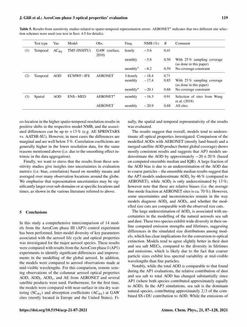
J. Gliß et al.: AeroCom phase 3 optical properties’ evaluation 119
Table 5. Results from sensitivity studies related to spatio-temporal representation errors. AERONET∗ indicates that two different site selec-tion schemes were used (see text in Sect. 4.5 for details).
Test type Var. Model Obs. Freq. NMB (%) R Comment
(1) Temporal ACdry TM5 (INSITU) GAW (surface,2010)
hourly −5.6 0.41
monthly −5.8 0.50 With 25 % sampling coverage(as done in this paper)
monthly∗ −8.2 0.59 No coverage constraint
(2) Temporal AOD ECMWF−IFS AERONET 3-hourly −18.4 0.71monthly −17.4 0.85 With 25 % sampling coverage
(as done in this paper)monthly∗ −20.1 0.68 No coverage constraint
(3) Spatial AOD ENS−MED AERONET∗ monthly −16.3 0.91 Selection of sites from Wanget al. (2018)
AERONET monthly −20.9 0.88 All sites
co-location in the higher spatio-temporal resolution results inpositive shifts in the respective model NMB, and the associ-ated differences can be up to +13 % (e.g. AE SPRINTARSvs. AATSR-SU). However, in most cases the differences aremarginal and are well below 5 %. Correlation coefficients aregenerally higher in the lower resolution data, for the samereasons mentioned above (i.e. due to the smoothing effect in-trinsic in the data aggregation).
Finally, we want to stress that the results from these sen-sitivity studies give insights into uncertainties in evaluationmetrics (i.e. bias, correlation) based on monthly means andaveraged over many observation locations around the globe.We emphasise that representation uncertainties may be sig-nificantly larger over sub-domains or at specific locations andtimes, as shown in the various literature referred to above.
5 Conclusions
In this study a comprehensive intercomparison of 14 mod-els from the AeroCom phase III (AP3) control experimenthas been performed. Inter-model diversity of key parametersassociated with the aerosol life cycle and optical propertieswas investigated for the major aerosol species. These resultswere compared with results from the AeroCom phase I (AP1)experiments to identify significant differences and improve-ments in the modelling of the global aerosol. In addition,the models were compared to aerosol observations made atmid-visible wavelengths. For this comparison, remote sens-ing observations of the columnar aerosol optical propertiesAOD, AODf, AODc, and AE from AERONET and severalsatellite products were used. Furthermore, for the first time,the models were compared with near-surface in situ dry scat-tering (SCdry) and absorption coefficients (ACdry) at GAWsites (mostly located in Europe and the United States). Fi-
nally, the spatial and temporal representativity of the resultswas evaluated.
The results suggest that overall, models tend to underes-timate all optical properties investigated. Comparison of themodelled AODs with AERONET (mostly land-based) and amerged satellite AOD product (better global coverage) showsmostly consistent results and suggests that AP3 models un-derestimate the AOD by approximately −20± 20 % (basedon computed ensemble median and IQR). A large fraction ofthe AOD bias is due to an underestimation of the AOD dueto coarse particles – the ensemble median results suggest thatthe AP3 models underestimate AODc by 46 % (compared toAERONET), while AODf is only underestimated by 13 %;however note that these are relative biases (i.e. the averagefine-mode fraction at AERONET sites is ca. 70 %). However,some uncertainties and inconsistencies remain in the waymodels diagnose AODc and AODf, and whether the mod-elled size cuts are comparable with the observed size cuts.
The large underestimation of AODc is associated with un-certainties in the modelling of the natural aerosols sea saltand dust. These two species exhibit wide diversity in their on-line computed emission strengths and lifetimes, suggestingdifferences in the simulated size distributions among mod-els, which has clear implications for the conversion to opticalextinction. Models tend to agree slightly better in their dustand sea salt MECs, compared to the diversity in lifetimesand emissions, which is likely due to the fact that coarserparticle sizes exhibit less spectral variability at mid-visiblewavelengths than fine particles.
Notably, while the total AOD is comparable to that foundduring the AP1 evaluations, the relative contribution of dustand sea salt to total AOD has changed substantially sinceAP1 (where both species contributed approximately equallyto AOD). In the AP3 simulations, sea salt is the dominantnatural species, contributing approximately 2/3 of the com-bined SS+DU contribution to AOD. While the emissions of
https://doi.org/10.5194/acp-21-87-2021 Atmos. Chem. Phys., 21, 87–128, 2021
120 J. Gliß et al.: AeroCom phase 3 optical properties’ evaluation
both species decrease in AP3, this shift in their relative con-tribution is mostly due to lifetime changes. In the case ofsea salt the emissions decrease is largely compensated for byan increase in its lifetime, which suggests that smaller seasalt particles are being simulated (or removal pathways areless efficient). On the other hand, the dust lifetime is slightlydecreased compared to AP1, resulting in a ca. 25 % lowerglobal dust burden.
Interestingly, the comparison of simulated AE with mea-surements of the AE from AERONET suggests that mod-els (still) simulate dust aerosol that is too fine or overes-timate the fine-mode fraction of coarse-dominated aerosol.This would likely translate into an overestimation of the dustMEC, which is, however, reduced compared to AP1 and de-serves further attention.
Unfortunately, a clear assessment of the modelled sea saltsize distributions based on the AE is difficult within the scopeof this paper. This is mostly due to a lack of ground-basedmeasurements over the oceans and large uncertainties in thesatellite AE data but also because of the impact of water up-take on the simulated size distributions. The longer sea saltlifetime compared to AP1 suggests smaller dry sea salt par-ticles in AP3 models, which has implications for water up-take and associated light scattering enhancement and possi-bly also for cloud formation and properties (e.g. cloud life-time and albedo) in clean marine environments. Indicationsfor and implications of smaller sea salt particles are reflectedin results from a few models showing above-average sea saltlifetimes, burdens, MECs, and water contribution to AOD,as well as overestimates (and decreased correlation) of totalAOD and AODc, particularly in comparison with the satel-lites over the oceans. An overestimated contribution of wa-ter uptake to the light extinction is also supported by a con-siderable underestimate and inter-model spread in the near-surface “dry” scattering coefficients, with a bias of approx-imately −35± 25 % found when comparing the ensemblemedian with GAW in situ aerosol scattering measurements.
Similar to AP1, the contribution of the other aerosolspecies (SO4, OA, and BC) to total AOD shows consider-able variability among the models, while the simulated totalAODs are more consistent. The AP3 SO4 life cycle and opti-cal parameters are mostly comparable with AP1. The sourcestrength of OA (POA + secondary formation) shows an in-crease of ca. 20 % relative to AP1, which translates into asimilar increase in its mass burden and the contribution ofOA to AOD. However, the contribution of OA to AOD ex-hibits large variability among the models, which is mostlydue to the fact that models that tend to simulate an above-average OA burden also show an above-average MEC andvice versa. The BC emissions are harmonised; however, lifecycle processes related to BC exhibit considerable diversity,resulting in a decrease in the BC mass burden by almosta factor of 2 compared to AP1, mostly due to a decreasein BC lifetime from 6.5 d in AP1 to 5.5 d in AP3. At thesame time BC MAC is slightly increased with a median of
8.5 m2/g in AP3 but is still lower than recommended litera-ture values. The results indicate improvement in the BC sizeassumptions and impacts of ageing (e.g. hygroscopicity dueto internal mixing or absorption enhancement effects) but arealso likely related to shifts in the assumed BC refractive in-dex towards more absorbing aerosol (in some models). Thesechanges from AP1 to AP3 reflect the considerable effort thatwent into improving models’ treatment of BC. However, con-sidering the finding of Samset et al. (2014), the BC lifetimein AP3 remains too long.
The lower BC burden is also reflected in considerable un-derestimations (bias ca. −20± 18 % based on ensemble andIQR) of the near-surface dry absorption coefficients at GAWsites. However, there is considerable diversity among the in-dividual 39 GAW sites considered (most of which are locatedin Europe), indicating impacts of transport and vertical mix-ing. The SCdry results show larger underestimates (−35 %)and more inter-model diversity than the ACdry comparisons.These results reflect uncertainties related to mixing and wa-ter uptake for scattering and – since the ambient AOD biasis less negative (−20 %) – are consistent with recent findingsby Burgos et al. (2020), indicating that current climate mod-els overestimate the light scattering enhancement associatedwith aerosol water uptake.
A detailed investigation of model biases compared toAERONET AE in different observed AE regimes sug-gests that models overestimate size (or underestimate thefine-mode fraction) in fine-mode-dominated regimes, whilecoarse-mode-dominated regimes indicate the opposite; thatis, models simulate particles that are not coarse enough (oroverestimate the contribution of fine aerosol to extinction).Even though the AERONET AE measurements are mostlyland-based, this could further indicate that not only the hy-drophobic dust but also sea salt particles are too small. Thiscould explain a possible overestimation of the light scatteringenhancement, which impacts fine particles more than coarseparticles (Zieger et al., 2013). However, we note that such ahypothesis would need to be investigated in more detail forthe AP3 models to make clear statements related to the seasalt size and water uptake.
The newly introduced NO3 aerosol component in 9 of the14 models exhibits very large variability in all life cycle andoptical parameters investigated, and it was shown that thisis mostly linked to differences in the assumed size distribu-tions but, to some degree, also due to inconsistencies in theassociated diagnostics submitted to AeroCom. However, theimpact of these uncertainties on total AOD is small as NO3contributes a small fraction to the total AOD (< 5 % basedon the median results of this study).
The quality of the constructed AeroCom median ensem-ble model is a very solid reference for the parameters inves-tigated. In terms of correlation, only in a few instances doindividual models outperform it; however no single model isbetter than the ensemble model for all parameters. This pa-per and its associated supplements, the AeroCom database,
Atmos. Chem. Phys., 21, 87–128, 2021 https://doi.org/10.5194/acp-21-87-2021
J. Gliß et al.: AeroCom phase 3 optical properties’ evaluation 121
and web interfaces are available as reference for further in-vestigations, in particular for developing recommendationsfor global aerosol modelling. Model diagnostics are compre-hensive but clearly not enough to understand all aspects ofhow models simulate the path from emissions to optical prop-erties. The documented inconsistencies in aerosol life cycleand mass to absorption/scattering coefficients are hopefullyan encouragement for modellers to further investigate theirindividual parameterisations and diagnostics.
The consistency of model performance against differentAOD observational data sets speaks in favour of the qual-ity of the observations. The performance variation againstdifferent AOD data sets provides at the same time a rougherror estimate or robustness of our evaluation method. Oursensitivity tests with respect to spatio-temporal resolutionand site selection indicate that the results are robust. Surfacein situ scattering and sun-photometer- and satellite-derivedAOD data have been used for the first time in a consis-tent way for evaluating a multi-model ensemble, revealingan underestimate of aerosol AOD, though smaller for an-thropogenic, fine-mode aerosol. Using fine-mode AOD as aproxy for present-day aerosol forcing estimates, our resultssuggest that models underestimate aerosol forcing by ca.−15 %. However, the associated inter-model spread (quan-tified by the IQR) is between −35 % and +10 % and sum-marises the large disparity between the individual models,stressing the need for further research.
In future studies the biases found in this study should beinvestigated, for instance, by incorporating additional aspectsinto the analysis such as model resolution (particularly verti-cal), regional and seasonal variations, profile extinction data,or column water content (to assess hygroscopic growth).Delving into the details of assumed size distributions, par-ticularly for natural aerosol, could also help resolve some ofthe discrepancies reported on here. In addition, a compar-ison with mass concentration measurements at the surfaceand aloft could provide valuable insights related to the ques-tion of whether the models are missing mass or whether as-sumptions about optical properties are causing the underesti-mated scattering coefficients and optical depth. Such an anal-ysis would certainly also benefit from a better global cover-age of surface measurement sites. The pre-industrial aerosolstate (although available in the AeroCom AP3 control exper-iment) has not been incorporated yet but should be includedto provide more insight into aerosol forcing estimates andlink these to the CMIP6 model ensemble results on historicalclimate evolution.
Code and data availability. Most of the data analysis was per-formed using the open-source software pyaerocom (version 0.10.0,https://doi.org/10.5281/zenodo.4362479, Gliß et al., 2020). All ad-ditional analysis scripts are stored in a private GitHub repositoryand can be provided upon request. All data used in this study arestored on servers of the Norwegian Meteorological Institute and
can be provided upon request. The GAW data used are accessiblethrough the EBAS database.
Supplement. The supplement related to this article is available on-line at: https://doi.org/10.5194/acp-21-87-2021-supplement.
Author contributions. JG, MS, and AM designed the study. JG didmost of the analysis and wrote most of the paper, together withsubstantial contributions from MS and EA. AM, JJG, and MS con-tributed the interactive websites associated with this study. EA, AH,PL, PN, CM, JJG, and LS helped to analyse and interpret the obser-vational data used. AB and JJG helped to organise the AeroComdatabase and AeroCom infrastructure needed. YB, SB, HB, RCG,MC, PG, ZK, AK, HK, PS, ML, HM, GM, DN, TN, DJLO, SR,TT, KT, and ST provided model data and model interpretations. Allco-authors gave feedback on the paper.
Competing interests. The authors declare that they have no conflictof interest.
Special issue statement. This article is part of the special is-sue “The Aerosol Chemistry Model Intercomparison Project(AerChemMIP)”. It is not associated with a conference.
Acknowledgements. Data providers from all observation networksand satellite products and all people involved in the production ofthese products are highly acknowledged for sharing and submit-ting their data and for support. Jonas Gliß wishes to thank Os-kar Landgren and Hanna Svennevik for providing data and codeused in this study and Stefan Kinne for helpful comments via per-sonal communication. Toshihiko Takemura was supported by thesupercomputer system of the National Institute for EnvironmentalStudies, Japan, Japan Society for the Promotion of Science (JSPS)KAKENHI (JP19H05669), and Environment Research and Tech-nology Development Fund (JPMEERF20202F01) of the Environ-mental Restoration and Conservation Agency, Japan. Twan vanNoije and Philippe Le Sager acknowledge funding from the Euro-pean Union’s Horizon 2020 Research and Innovation programme,project CRESCENDO (Coordinated Research in Earth Systems andClimate: Experiments, Knowledge, Dissemination and Outreach),under grant agreement no. 641816. David Neubauer acknowledgesfunding from the European Union’s Horizon 2020 Research andInnovation programme, project FORCeS, under grant agreementno. 821205. Susanne E. Bauer and Kostas Tsigaridis acknowl-edge funding from NASA’s Atmospheric Composition Modelingand Analysis Program (ACMAP), contract number NNX15AE36G.Paul Ginoux acknowledges partial funding from NASA’s Earth Sur-face Mineral Dust Source Investigation (EMIT), program numberNNH12ZDA0060-EVI4. They also thank Jingbo Yu for runningthe GISS model. Resources supporting this work were providedby the NASA High-End Computing (HEC) Program through theNASA Center for Climate Simulation (NCCS) at Goddard SpaceFlight Center. Harri Kokkola acknowledges the Academy of Fin-land Projects 317390 and 308292. The ECHAM-HAMMOZ model
https://doi.org/10.5194/acp-21-87-2021 Atmos. Chem. Phys., 21, 87–128, 2021
122 J. Gliß et al.: AeroCom phase 3 optical properties’ evaluation
is developed by a consortium composed of ETH Zurich, Max-Planck-Institut für Meteorologie, Forschungszentrum Jülich, Uni-versity of Oxford, the Finnish Meteorological Institute, and theLeibniz Institute for Tropospheric Research and managed by theCenter for Climate Systems Modeling (C2SM) at ETH Zurich. Pe-ter North and Andreas Heckel are supported by the ESA AerosolClimate Change Initiative (Aerosol CCI). Hitoshi Matsui acknowl-edges funding from the Ministry of Education, Culture, Sports, Sci-ence, and Technology and the Japan Society for the Promotion ofScience (MEXT/JSPS) KAKENHI (grant no. JP17H04709). Gun-nar Myhre has received support from project SUPER (grant no.250573), funded by the Research Council of Norway. HuishengBian acknowledges funding from NASA’s Atmospheric Compo-sition Modeling and Analysis Program (ACMAP), contract no.NNX17AG31G. Mian Chin acknowledges support by the NASAEarth Science programs. We thank two anonymous reviewers forcareful reading and constructive suggestions.
Financial support. This research has been supported by the Re-search Council of Norway (EVA (grant no. 229771), INES (grantno. 270061), and KeyClim (grant no. 295046)) and the Hori-zon 2020 project CRESCENDO (grant no. 641816). High per-formance computing and storage resources were provided bythe Norwegian Infrastructure for Computational Science (throughprojects NN2345K, NN9560K, NS2345K, and NS9560K). Pleasealso note further funding sources in the Acknowledgements.
Review statement. This paper was edited by Nikolaos Mihalopou-los and reviewed by two anonymous referees.
References
Aas, W., Mortier, A., Bowersox, V., Cherian, R., Faluvegi, G.,Fagerli, H., Hand, J., Klimont, Z., Galy-Lacaux, C., Lehmann,C. M. B., Myhre, C. L., Myhre, G., Olivié, D., Sato, K.,Quaas, J., Rao, P. S. P., Schulz, M., Shindell, D., Skeie, R. B.,Stein, A., Takemura, T., Tsyro, S., Vet, R., and Xu, X.: Globaland regional trends of atmospheric sulfur, Sci. Rep., 9, 953,https://doi.org/10.1038/s41598-018-37304-0, 2019.
AeroCom diagnostics sheet: AeroCom diagnostics sheet,available at: https://docs.google.com/spreadsheets/d/1NiHLVTDsBo0JEBSnnDECNI2ojUnCVlxuy2PFrsRJW38/edit?usp=sharing, last access: 19 August 2020.
AeroCom wiki: AeroCom Phase III experiments description, avail-able at: https://wiki.met.no/aerocom/phase3-experiments, lastaccess: 22 August 2020.
Andres, R. J. and Kasgnoc, A. D.: A time-averaged inventory ofsubaerial volcanic sulfur emissions, J. Geophys. Res.-Atmos.,103, 25251–25261, https://doi.org/10.1029/98JD02091, 1998.
Andrews, E., Sheridan, P. J., Ogren, J. A., Hageman, D., Jeffer-son, A., Wendell, J., Alástuey, A., Alados-Arboledas, L., Bergin,M., Ealo, M., Hallar, A. G., Hoffer, A., Kalapov, I., Key-wood, M., Kim, J., Kim, S.-W., Kolonjari, F., Labuschagne, C.,Lin, N.-H., Macdonald, A., Mayol-Bracero, O. L., McCubbin,I. B., Pandolfi, M., Reisen, F., Sharma, S., Sherman, J. P., Sor-ribas, M., and Sun, J.: Overview of the NOAA/ESRL Feder-
ated Aerosol Network, B. Am. Meteorol. Soc., 100, 123–135,https://doi.org/10.1175/BAMS-D-17-0175.1, 2019.
Balkanski, Y., Schulz, M., Claquin, T., Moulin, C., and Gi-noux, P.: Global Emissions of Mineral Aerosol: Formula-tion and Validation using Satellite Imagery, in: Advancesin Global Change Research, Springer Netherlands, 239–267,https://doi.org/10.1007/978-1-4020-2167-1_6, 2004.
Bergman, T., Kerminen, V.-M., Korhonen, H., Lehtinen, K. J.,Makkonen, R., Arola, A., Mielonen, T., Romakkaniemi, S., Kul-mala, M., and Kokkola, H.: Evaluation of the sectional aerosolmicrophysics module SALSA implementation in ECHAM5-HAM aerosol-climate model, Geosci. Model Dev., 5, 845–868,https://doi.org/10.5194/gmd-5-845-2012, 2012.
Bevan, S. L., North, P. R. J., Los, S. O., and Grey, W. M. F.: Aglobal dataset of atmospheric aerosol optical depth and surfacereflectance from AATSR, Remote Sens. Environ., 116, 199–210,https://doi.org/10.1016/j.rse.2011.05.024, 2012.
Bian, H., Chin, M., Hauglustaine, D. A., Schulz, M., Myhre, G.,Bauer, S. E., Lund, M. T., Karydis, V. A., Kucsera, T. L., Pan, X.,Pozzer, A., Skeie, R. B., Steenrod, S. D., Sudo, K., Tsigaridis,K., Tsimpidi, A. P., and Tsyro, S. G.: Investigation of global par-ticulate nitrate from the AeroCom phase III experiment, Atmos.Chem. Phys., 17, 12911–12940, https://doi.org/10.5194/acp-17-12911-2017, 2017.
Bian, H., Froyd, K., Murphy, D. M., Dibb, J., Darmenov, A.,Chin, M., Colarco, P. R., da Silva, A., Kucsera, T. L., Schill,G., Yu, H., Bui, P., Dollner, M., Weinzierl, B., and Smirnov,A.: Observationally constrained analysis of sea salt aerosol inthe marine atmosphere, Atmos. Chem. Phys., 19, 10773–10785,https://doi.org/10.5194/acp-19-10773-2019, 2019.
Bond, T. C. and Bergstrom, R. W.: Light Absorption by Carbona-ceous Particles: An Investigative Review, Aerosol Sci. Tech., 40,27–67, https://doi.org/10.1080/02786820500421521, 2006.
Bond, T. C., Doherty, S. J., Fahey, D. W., Forster, P. M., Berntsen,T., DeAngelo, B. J., Flanner, M. G., Ghan, S., Kärcher, B.,Koch, D., Kinne, S., Kondo, Y., Quinn, P. K., Sarofim, M. C.,Schultz, M. G., Schulz, M., Venkataraman, C., Zhang, H., Zhang,S., Bellouin, N., Guttikunda, S. K., Hopke, P. K., Jacobson,M. Z., Kaiser, J. W., Klimont, Z., Lohmann, U., Schwarz, J. P.,Shindell, D., Storelvmo, T., Warren, S. G., and Zender, C. S.:Bounding the role of black carbon in the climate system: A sci-entific assessment, J. Geophys. Res.-Atmos., 118, 5380–5552,https://doi.org/10.1002/jgrd.50171, 2013.
Boucher, O., Randall, D., Artaxo, P., Bretherton, C., Feingold, G.,Forster, P., Kerminen, V.-M., Kondo, Y., Liao, H., Lohmann, U.,Rasch, P., Satheesh, S., Sherwood, S., Stevens, B., and Zhang,X.: Clouds and Aerosols, book sect. 7, 571–658, Cambridge Uni-versity Press, Cambridge, United Kingdom and New York, NY,USA, https://doi.org/10.1017/CBO9781107415324.016, 2013.
Burgos, M. A., Andrews, E., Titos, G., Benedetti, A., Bian, H.,Buchard, V., Curci, G., Kipling, Z., Kirkevåg, A., Kokkola,H., Laakso, A., Letertre-Danczak, J., Lund, M. T., Matsui, H.,Myhre, G., Randles, C., Schulz, M., van Noije, T., Zhang, K.,Alados-Arboledas, L., Baltensperger, U., Jefferson, A., Sherman,J., Sun, J., Weingartner, E., and Zieger, P.: A global model–measurement evaluation of particle light scattering coefficientsat elevated relative humidity, Atmos. Chem. Phys., 20, 10231–10258, https://doi.org/10.5194/acp-20-10231-2020, 2020.
Atmos. Chem. Phys., 21, 87–128, 2021 https://doi.org/10.5194/acp-21-87-2021
https://docs.google.com/spreadsheets/d/1NiHLVTDsBo0JEBSnnDECNI2ojUnCVlxuy2PFrsRJW38/edit?usp=sharing
https://docs.google.com/spreadsheets/d/1NiHLVTDsBo0JEBSnnDECNI2ojUnCVlxuy2PFrsRJW38/edit?usp=sharing

J. Gliß et al.: AeroCom phase 3 optical properties’ evaluation 123
Cappa, C. D., Onasch, T. B., Massoli, P., Worsnop, D. R., Bates,T. S., Cross, E. S., Davidovits, P., Hakala, J., Hayden, K. L.,Jobson, B. T., Kolesar, K. R., Lack, D. A., Lerner, B. M., Li,S.-M., Mellon, D., Nuaaman, I., Olfert, J. S., Petäjä, T., Quinn,P. K., Song, C., Subramanian, R., Williams, E. J., and Zaveri,R. A.: Radiative Absorption Enhancements Due to the MixingState of Atmospheric Black Carbon, Science, 337, 1078–1081,https://doi.org/10.1126/science.1223447, 2012.
Carn, S. A., Fioletov, V. E., McLinden, C. A., Li, C.,and Krotkov, N. A.: A decade of global volcanic SO2emissions measured from space, Sci. Repo., 7, 44095,https://doi.org/10.1038/srep44095, 2017.
Carslaw, K. S., Lee, L. A., Reddington, C. L., Pringle, K. J., Rap,A., Forster, P. M., Mann, G. W., Spracklen, D. V., Woodhouse,M. T., Regayre, L. A., and Pierce, J. R.: Large contribution ofnatural aerosols to uncertainty in indirect forcing, Nature, 503,67–71, https://doi.org/10.1038/nature12674, 2013.
Claquin, T., Schulz, M., Balkanski, Y., and Boucher, O.: Uncer-tainties in assessing radiative forcing by mineral dust, TellusB, 50, 491–505, https://doi.org/10.1034/j.1600-0889.1998.t01-2-00007.x, 1998.
Colarco, P., da Silva, A., Chin, M., and Diehl, T.: Onlinesimulations of global aerosol distributions in the NASAGEOS-4 model and comparisons to satellite and ground-basedaerosol optical depth, J. Geophys. Res.-Atmos., 115, D14207,https://doi.org/10.1029/2009JD012820, 2010.
Collaud Coen, M., Andrews, E., Alastuey, A., Arsov, T. P., Back-man, J., Brem, B. T., Bukowiecki, N., Couret, C., Eleftheri-adis, K., Flentje, H., Fiebig, M., Gysel-Beer, M., Hand, J. L.,Hoffer, A., Hooda, R., Hueglin, C., Joubert, W., Keywood, M.,Kim, J. E., Kim, S.-W., Labuschagne, C., Lin, N.-H., Lin, Y.,Lund Myhre, C., Luoma, K., Lyamani, H., Marinoni, A., Mayol-Bracero, O. L., Mihalopoulos, N., Pandolfi, M., Prats, N., Prenni,A. J., Putaud, J.-P., Ries, L., Reisen, F., Sellegri, K., Sharma,S., Sheridan, P., Sherman, J. P., Sun, J., Titos, G., Torres, E.,Tuch, T., Weller, R., Wiedensohler, A., Zieger, P., and Laj, P.:Multidecadal trend analysis of in situ aerosol radiative prop-erties around the world, Atmos. Chem. Phys., 20, 8867–8908,https://doi.org/10.5194/acp-20-8867-2020, 2020.
de Leeuw, G., Holzer-Popp, T., Bevan, S., Davies, W. H., De-scloitres, J., Grainger, R. G., Griesfeller, J., Heckel, A., Kinne,S., Klüser, L., Kolmonen, P., Litvinov, P., Martynenko, D., North,P., Ovigneur, B., Pascal, N., Poulsen, C., Ramon, D., Schulz, M.,Siddans, R., Sogacheva, L., Tanré, D., Thomas, G. E., Virtanen,T. H., von Hoyningen Huene, W., Vountas, M., and Pinnock, S.:Evaluation of seven European aerosol optical depth retrieval al-gorithms for climate analysis, Remote Sens. Environ., 162, 295–315, https://doi.org/10.1016/j.rse.2013.04.023, 2015.
Dentener, F., Kinne, S., Bond, T., Boucher, O., Cofala, J., Gen-eroso, S., Ginoux, P., Gong, S., Hoelzemann, J. J., Ito, A.,Marelli, L., Penner, J. E., Putaud, J.-P., Textor, C., Schulz, M.,van der Werf, G. R., and Wilson, J.: Emissions of primaryaerosol and precursor gases in the years 2000 and 1750 pre-scribed data-sets for AeroCom, Atmos. Chem. Phys., 6, 4321–4344, https://doi.org/10.5194/acp-6-4321-2006, 2006.
Dubovik, O. and King, M. D.: A flexible inversion algorithm for re-trieval of aerosol optical properties from Sun and sky radiancemeasurements, J. Geophys. Res.-Atmos., 105, 20673–20696,https://doi.org/10.1029/2000JD900282, 2000.
ERA5: Copernicus Climate Change Service (C3S) (2017): ERA5:Fifth generation of ECMWF atmospheric reanalyses of theglobal climate, Copernicus Climate Change Service ClimateData Store (CDS), available at: https://cds.climate.copernicus.eu/cdsapp#!/home, last access: 27 December 2019.
Eyring, V., Bony, S., Meehl, G. A., Senior, C. A., Stevens, B.,Stouffer, R. J., and Taylor, K. E.: Overview of the CoupledModel Intercomparison Project Phase 6 (CMIP6) experimen-tal design and organization, Geosci. Model Dev., 9, 1937–1958,https://doi.org/10.5194/gmd-9-1937-2016, 2016.
Fossum, K. N., Ovadnevaite, J., Ceburnis, D., Preißler, J., Snider,J. R., Huang, R.-J., Zuend, A., and O’Dowd, C.: Sea-spray reg-ulates sulfate cloud droplet activation over oceans, npj Clim.Atmos. Sci., 3, 14, https://doi.org/10.1038/s41612-020-0116-2,2020.
GAW Report 227: WMO/GAW Aerosol Measurement Proce-dures, Guidelines and Recommendations, available at: https://library.wmo.int/doc_num.php?explnum_id=3073 (last access:14 September 2020), 2016.
Giles, D. M., Sinyuk, A., Sorokin, M. G., Schafer, J. S., Smirnov,A., Slutsker, I., Eck, T. F., Holben, B. N., Lewis, J. R., Campbell,J. R., Welton, E. J., Korkin, S. V., and Lyapustin, A. I.: Advance-ments in the Aerosol Robotic Network (AERONET) Version 3database – automated near-real-time quality control algorithmwith improved cloud screening for Sun photometer aerosol op-tical depth (AOD) measurements, Atmos. Meas. Tech., 12, 169–209, https://doi.org/10.5194/amt-12-169-2019, 2019.
Gliß, J.: Geonum python library, available at: https://geonum.readthedocs.io/en/latest (last access: 20 August 2020), 2017.
Gliß, J., Gallefoss, E., Brenna, H., Griesfeller, J., Mortier,A., Svennevik, H., Sjur, A.-L., and Schulz, M.:metno/pyaerocom: Version 0.10.0 (Version v0.10.0), Zen-odo, https://doi.org/10.5281/zenodo.4362479, 2020.
Grythe, H., Ström, J., Krejci, R., Quinn, P., and Stohl, A.: A re-view of sea-spray aerosol source functions using a large globalset of sea salt aerosol concentration measurements, Atmos.Chem. Phys., 14, 1277–1297, https://doi.org/10.5194/acp-14-1277-2014, 2014.
Guelle, W., Schulz, M., Balkanski, Y., and Dentener, F.: Influenceof the source formulation on modeling the atmospheric globaldistribution of sea salt aerosol, J. Geophys. Res.-Atmos., 106,27509–27524, https://doi.org/10.1029/2001JD900249, 2001.
Gupta, P., Remer, L. A., Levy, R. C., and Mattoo, S.: Validationof MODIS 3 km land aerosol optical depth from NASA’s EOSTerra and Aqua missions, Atmos. Meas. Tech., 11, 3145–3159,https://doi.org/10.5194/amt-11-3145-2018, 2018.
Halmer, M. M., Schmincke, H. U., and Graf, H. F.: The annual vol-canic gas input into the atmosphere, in particular into the strato-sphere: A global data set for the past 100 years, J. Volcanol.Geoth. Res., 115, 511–528, https://doi.org/10.1016/S0377-0273(01)00318-3, 2002.
Hand, J. L. and Malm, W. C.: Review of aerosol massscattering efficiencies from ground-based measurementssince 1990, J. Geophys. Res.-Atmos., 112, D16203,https://doi.org/10.1029/2007JD008484, 2007.
Hoesly, R. M., Smith, S. J., Feng, L., Klimont, Z., Janssens-Maenhout, G., Pitkanen, T., Seibert, J. J., Vu, L., Andres, R.J., Bolt, R. M., Bond, T. C., Dawidowski, L., Kholod, N.,Kurokawa, J.-I., Li, M., Liu, L., Lu, Z., Moura, M. C. P.,
https://doi.org/10.5194/acp-21-87-2021 Atmos. Chem. Phys., 21, 87–128, 2021
124 J. Gliß et al.: AeroCom phase 3 optical properties’ evaluation
O’Rourke, P. R., and Zhang, Q.: Historical (1750–2014) anthro-pogenic emissions of reactive gases and aerosols from the Com-munity Emissions Data System (CEDS), Geosci. Model Dev., 11,369–408, https://doi.org/10.5194/gmd-11-369-2018, 2018.
Holben, B. N., Eck, T. F., Slutsker, I., Tanré, D., Buis,J. P., Setzer, A., Vermote, E., Reagan, J. A., Kaufman,Y. J., Nakajima, T., Lavenu, F., Jankowiak, I., and Smirnov,A.: AERONET—A Federated Instrument Network and DataArchive for Aerosol Characterization, Remote Sens. Envi-ron., 66, 1–16, https://doi.org/10.1016/S0034-4257(98)00031-5,1998.
Holben, B. N., Kim, J., Sano, I., Mukai, S., Eck, T. F., Giles, D.M., Schafer, J. S., Sinyuk, A., Slutsker, I., Smirnov, A., Sorokin,M., Anderson, B. E., Che, H., Choi, M., Crawford, J. H., Ferrare,R. A., Garay, M. J., Jeong, U., Kim, M., Kim, W., Knox, N., Li,Z., Lim, H. S., Liu, Y., Maring, H., Nakata, M., Pickering, K. E.,Piketh, S., Redemann, J., Reid, J. S., Salinas, S., Seo, S., Tan,F., Tripathi, S. N., Toon, O. B., and Xiao, Q.: An overview ofmesoscale aerosol processes, comparisons, and validation studiesfrom DRAGON networks, Atmos. Chem. Phys., 18, 655–671,https://doi.org/10.5194/acp-18-655-2018, 2018.
Hsu, N. C., Tsay, S.-C., King, M. D., and Herman,J. R.: Aerosol properties over bright-reflecting sourceregions, IEEE T. Geosci. Remote S., 42, 557–569,https://doi.org/10.1109/TGRS.2004.824067, 2004.
Hubanks, P. A.: Collection 6.1Change Summary Document-MODIS Atmosphere Level-3 Algorithmand Global Products,Tech. rep., available at: https://atmosphere-imager.gsfc.nasa.gov/sites/default/files/ModAtmo/L3_C61_Changes_v2.pdf (last ac-cess: 21 December 2020), 2017.
Huneeus, N., Schulz, M., Balkanski, Y., Griesfeller, J., Prospero,J., Kinne, S., Bauer, S., Boucher, O., Chin, M., Dentener, F.,Diehl, T., Easter, R., Fillmore, D., Ghan, S., Ginoux, P., Grini,A., Horowitz, L., Koch, D., Krol, M. C., Landing, W., Liu,X., Mahowald, N., Miller, R., Morcrette, J.-J., Myhre, G., Pen-ner, J., Perlwitz, J., Stier, P., Takemura, T., and Zender, C. S.:Global dust model intercomparison in AeroCom phase I, At-mos. Chem. Phys., 11, 7781–7816, https://doi.org/10.5194/acp-11-7781-2011, 2011.
IPCC: Climate Change 2013: The Physical Science Basis. Contri-bution of Working Group I to the Fifth Assessment Report of theIntergovernmental Panel on Climate Change, edited by: Stocker,T. F., Qin, D., Plattner, G.-K., Tignor, M., Allen, S. K., Boschung,J., Nauels, A., Xia, Y., Bex, V., and Midgley, P. M., CambridgeUniversity Press, Cambridge, United Kingdom and New York,NY, USA, 1535 pp., 2013.
Kandler, K., Benker, N., Bundke, U., Cuevas, E., Ebert, M.,Knippertz, P., Rodríguez, S., Schütz, L., and Weinbruch,S.: Chemical composition and complex refractive index ofSaharan Mineral Dust at Izaña, Tenerife (Spain) derivedby electron microscopy, Atmos. Environ., 41, 8058–8074,https://doi.org/10.1016/j.atmosenv.2007.06.047, 2007.
Kiehl, J. T. and Briegleb, B. P.: The Relative Roles of SulfateAerosols and Greenhouse Gases in Climate Forcing, Science,260, 311–314, https://doi.org/10.1126/science.260.5106.311,1993.
Kim, D., Chin, M., Yu, H., Diehl, T., Tan, Q., Kahn, R. A.,Tsigaridis, K., Bauer, S. E., Takemura, T., Pozzoli, L., Bel-louin, N., Schulz, M., Peyridieu, S., Chédin, A., and Koffi,
B.: Sources, sinks, and transatlantic transport of North Africandust aerosol: A multimodel analysis and comparison with re-mote sensing data, J. Geophys. Res.-Atmos., 119, 6259–6277,https://doi.org/10.1002/2013JD021099, 2014.
Kinne, S., Schulz, M., Textor, C., Guibert, S., Balkanski, Y., Bauer,S. E., Berntsen, T., Berglen, T. F., Boucher, O., Chin, M., Collins,W., Dentener, F., Diehl, T., Easter, R., Feichter, J., Fillmore, D.,Ghan, S., Ginoux, P., Gong, S., Grini, A., Hendricks, J., Herzog,M., Horowitz, L., Isaksen, I., Iversen, T., Kirkevåg, A., Kloster,S., Koch, D., Kristjansson, J. E., Krol, M., Lauer, A., Lamarque,J. F., Lesins, G., Liu, X., Lohmann, U., Montanaro, V., Myhre,G., Penner, J., Pitari, G., Reddy, S., Seland, O., Stier, P., Take-mura, T., and Tie, X.: An AeroCom initial assessment – opticalproperties in aerosol component modules of global models, At-mos. Chem. Phys., 6, 1815–1834, https://doi.org/10.5194/acp-6-1815-2006, 2006.
Kinne, S., O’Donnel, D., Stier, P., Kloster, S., Zhang, K.,Schmidt, H., Rast, S., Giorgetta, M., Eck, T. F., andStevens, B.: MAC-v1: A new global aerosol climatologyfor climate studies, J. Adv. Model. Earth Sy., 5, 704–740,https://doi.org/10.1002/jame.20035, 2013.
Kirkevåg, A., Grini, A., Olivié, D., Seland, Ø., Alterskjær,K., Hummel, M., Karset, I. H. H., Lewinschal, A., Liu,X., Makkonen, R., Bethke, I., Griesfeller, J., Schulz, M.,and Iversen, T.: A production-tagged aerosol module forEarth system models, OsloAero5.3 – extensions and up-dates for CAM5.3-Oslo, Geosci. Model Dev., 11, 3945–3982,https://doi.org/10.5194/gmd-11-3945-2018, 2018.
Klimont, Z., Smith, S. J., and Cofala, J.: The last decadeof global anthropogenic sulfur dioxide: 2000-2011 emissions,Environ. Res. Lett., 8, 14003, https://doi.org/10.1088/1748-9326/8/1/014003, 2013.
Koch, D., Schmidt, G. A., and Field, C. V.: Sulfur, sea salt, andradionuclide aerosols in GISS ModelE, J. Geophys. Res.-Atmos.,111, D06206, https://doi.org/10.1029/2004JD005550, 2006.
Koch, D., Bond, T. C., Streets, D., Unger, N., and van der Werf,G. R.: Global impacts of aerosols from particular source re-gions and sectors, J. Geophys. Res.-Atmos., 112, D02205,https://doi.org/10.1029/2005JD007024, 2007.
Koch, D., Schulz, M., Kinne, S., McNaughton, C., Spackman, J.R., Balkanski, Y., Bauer, S., Berntsen, T., Bond, T. C., Boucher,O., Chin, M., Clarke, A., De Luca, N., Dentener, F., Diehl, T.,Dubovik, O., Easter, R., Fahey, D. W., Feichter, J., Fillmore,D., Freitag, S., Ghan, S., Ginoux, P., Gong, S., Horowitz, L.,Iversen, T., Kirkevåg, A., Klimont, Z., Kondo, Y., Krol, M., Liu,X., Miller, R., Montanaro, V., Moteki, N., Myhre, G., Penner,J. E., Perlwitz, J., Pitari, G., Reddy, S., Sahu, L., Sakamoto, H.,Schuster, G., Schwarz, J. P., Seland, Ø., Stier, P., Takegawa, N.,Takemura, T., Textor, C., van Aardenne, J. A., and Zhao, Y.: Eval-uation of black carbon estimations in global aerosol models, At-mos. Chem. Phys., 9, 9001–9026, https://doi.org/10.5194/acp-9-9001-2009, 2009.
Kok, J. F.: A scaling theory for the size distribution of emitted dustaerosols suggests climate models underestimate the size of theglobal dust cycle, P. Natl. Acad. Sci. USA, 108, 1016–1021,https://doi.org/10.1073/pnas.1014798108, 2011.
Kokkola, H., Kühn, T., Laakso, A., Bergman, T., Lehtinen, K.E. J., Mielonen, T., Arola, A., Stadtler, S., Korhonen, H., Fer-rachat, S., Lohmann, U., Neubauer, D., Tegen, I., Siegenthaler-
Atmos. Chem. Phys., 21, 87–128, 2021 https://doi.org/10.5194/acp-21-87-2021
J. Gliß et al.: AeroCom phase 3 optical properties’ evaluation 125
Le Drian, C., Schultz, M. G., Bey, I., Stier, P., Daskalakis,N., Heald, C. L., and Romakkaniemi, S.: SALSA2.0: The sec-tional aerosol module of the aerosol–chemistry–climate modelECHAM6.3.0-HAM2.3-MOZ1.0, Geosci. Model Dev., 11,3833–3863, https://doi.org/10.5194/gmd-11-3833-2018, 2018.
Lafon, S., Sokolik, I. N., Rajot, J. L., Caquineau, S., and Gaudichet,A.: Characterization of iron oxides in mineral dust aerosols: Im-plications for light absorption, J. Geophys. Res.-Atmos., 111,D21207, https://doi.org/10.1029/2005JD007016, 2006.
Laj, P., Bigi, A., Rose, C., Andrews, E., Lund Myhre, C., CollaudCoen, M., Lin, Y., Wiedensohler, A., Schulz, M., Ogren, J. A.,Fiebig, M., Gliß, J., Mortier, A., Pandolfi, M., Petäja, T., Kim,S.-W., Aas, W., Putaud, J.-P., Mayol-Bracero, O., Keywood,M., Labrador, L., Aalto, P., Ahlberg, E., Alados Arboledas, L.,Alastuey, A., Andrade, M., Artíñano, B., Ausmeel, S., Arsov, T.,Asmi, E., Backman, J., Baltensperger, U., Bastian, S., Bath, O.,Beukes, J. P., Brem, B. T., Bukowiecki, N., Conil, S., Couret,C., Day, D., Dayantolis, W., Degorska, A., Eleftheriadis, K., Fet-fatzis, P., Favez, O., Flentje, H., Gini, M. I., Gregoric, A., Gysel-Beer, M., Hallar, A. G., Hand, J., Hoffer, A., Hueglin, C., Hooda,R. K., Hyvärinen, A., Kalapov, I., Kalivitis, N., Kasper-Giebl,A., Kim, J. E., Kouvarakis, G., Kranjc, I., Krejci, R., Kulmala,M., Labuschagne, C., Lee, H.-J., Lihavainen, H., Lin, N.-H.,Löschau, G., Luoma, K., Marinoni, A., Martins Dos Santos, S.,Meinhardt, F., Merkel, M., Metzger, J.-M., Mihalopoulos, N.,Nguyen, N. A., Ondracek, J., Pérez, N., Perrone, M. R., Petit,J.-E., Picard, D., Pichon, J.-M., Pont, V., Prats, N., Prenni, A.,Reisen, F., Romano, S., Sellegri, K., Sharma, S., Schauer, G.,Sheridan, P., Sherman, J. P., Schütze, M., Schwerin, A., Sohmer,R., Sorribas, M., Steinbacher, M., Sun, J., Titos, G., Toczko, B.,Tuch, T., Tulet, P., Tunved, P., Vakkari, V., Velarde, F., Velasquez,P., Villani, P., Vratolis, S., Wang, S.-H., Weinhold, K., Weller,R., Yela, M., Yus-Diez, J., Zdimal, V., Zieger, P., and Zikova,N.: A global analysis of climate-relevant aerosol properties re-trieved from the network of Global Atmosphere Watch (GAW)near-surface observatories, Atmos. Meas. Tech., 13, 4353–4392,https://doi.org/10.5194/amt-13-4353-2020, 2020.
Latimer, R. N. C. and Martin, R. V.: Interpretation of measuredaerosol mass scattering efficiency over North America using achemical transport model, Atmos. Chem. Phys., 19, 2635–2653,https://doi.org/10.5194/acp-19-2635-2019, 2019.
Laurent, B., Marticorena, B., Bergametti, G., Léon, J. F.,and Mahowald, N. M.: Modeling mineral dust emissionsfrom the Sahara desert using new surface properties andsoil database, J. Geophys. Res.-Atmos., 113, D14218,https://doi.org/10.1029/2007JD009484, 2008.
Leaitch, W. R., Kodros, J. K., Willis, M. D., Hanna, S., Schulz,H., Andrews, E., Bozem, H., Burkart, J., Hoor, P., Kolonjari, F.,Ogren, J. A., Sharma, S., Si, M., von Salzen, K., Bertram, A. K.,Herber, A., Abbatt, J. P. D., and Pierce, J. R.: Vertical profilesof light absorption and scattering associated with black carbonparticle fractions in the springtime Arctic above 79° N, Atmos.Chem. Phys., 20, 10545–10563, https://doi.org/10.5194/acp-20-10545-2020, 2020.
Levy, R. C., Mattoo, S., Munchak, L. A., Remer, L. A., Sayer, A.M., Patadia, F., and Hsu, N. C.: The Collection 6 MODIS aerosolproducts over land and ocean, Atmos. Meas. Tech., 6, 2989–3034, https://doi.org/10.5194/amt-6-2989-2013, 2013.
Li, F., Ginoux, P., and Ramaswamy, V.: Distribution, transport, anddeposition of mineral dust in the Southern Ocean and Antarc-tica: Contribution of major sources, J. Geophys. Res.-Atmos.,113, D10207, https://doi.org/10.1029/2007JD009190, 2008.
Liu, D., Whitehead, J., Alfarra, M. R., Reyes-Villegas, E.,Spracklen, D. V., Reddington, C. L., Kong, S., Williams, P. I.,Ting, Y.-C., Haslett, S., et al.: Black-carbon absorption enhance-ment in the atmosphere determined by particle mixing state, Nat.Geosci., 10, 184–188, 2017.
Liu, F., Yon, J., Fuentes, A., Lobo, P., Smallwood, G. J., and Corbin,J. C.: Review of recent literature on the light absorption prop-erties of black carbon: Refractive index, mass absorption crosssection, and absorption function, Aerosol Sci. Tech., 54, 33–51,https://doi.org/10.1080/02786826.2019.1676878, 2020.
Lund, M. T., Myhre, G., Haslerud, A. S., Skeie, R. B., Gries-feller, J., Platt, S. M., Kumar, R., Myhre, C. L., and Schulz,M.: Concentrations and radiative forcing of anthropogenicaerosols from 1750 to 2014 simulated with the Oslo CTM3 andCEDS emission inventory, Geosci. Model Dev., 11, 4909–4931,https://doi.org/10.5194/gmd-11-4909-2018, 2018.
Matsui, H.: Development of a global aerosol model us-ing a two-dimensional sectional method: 1. Modeldesign, J. Adv. Model. Earth Sy., 9, 1921–1947,https://doi.org/10.1002/2017MS000936, 2017.
Matsui, H. and Mahowald, N.: Development of a global aerosolmodel using a two-dimensional sectional method: 2. Evaluationand sensitivity simulations, J. Adv. Model. Earth Sy.s, 9, 1887–1920, https://doi.org/10.1002/2017MS000937, 2017.
Matsui, H., Hamilton, D. S., and Mahowald, N. M.: Black car-bon radiative effects highly sensitive to emitted particle sizewhen resolving mixing-state diversity, Nat. Commun., 9, 3446,https://doi.org/10.1038/s41467-018-05635-1, 2018.
Mielonen, T., Portin, H., Komppula, M., Leskinen, A., Tam-minen, J., Ialongo, I., Hakkarainen, J., Lehtinen, K., andArola, A.: Biomass burning aerosols observed in EasternFinland during the Russian wildfires in summer 2010 –Part 2: Remote sensing, Atmos. Environ., 47, 279–287,https://doi.org/10.1016/j.atmosenv.2011.07.016, 2012.
Mortier, A., Gliß, J., and Schulz, M.: AeroCom web visualisation(Satellite evaluation), available at: https://aerocom-evaluation.met.no/overall.php?project=satellite&exp=eval2019, last access:14 September 2020a.
Mortier, A., Gliß, J., Schulz, M., Aas, W., Andrews, E., Bian, H.,Chin, M., Ginoux, P., Hand, J., Holben, B., Zhang, H., Kipling,Z., Kirkevåg, A., Laj, P., Lurton, T., Myhre, G., Neubauer, D.,Olivié, D., von Salzen, K., Skeie, R. B., Takemura, T., andTilmes, S.: Evaluation of climate model aerosol trends withground-based observations over the last 2 decades – an AeroComand CMIP6 analysis, Atmos. Chem. Phys., 20, 13355–13378,https://doi.org/10.5194/acp-20-13355-2020, 2020b.
Mortier, A., Gliß, J., Schulz, M., and community: AeroCom webvisualisation, online visualisation of results from Gliß et al.(acp-2019-1214), available at: https://aerocom-evaluation.met.no/main.php?project=aerocom&exp=glissetal-2020 (last access:21 December 2020), 2020c.
Myhre, G., Berglen, T. F., Johnsrud, M., Hoyle, C. R., Berntsen, T.K., Christopher, S. A., Fahey, D. W., Isaksen, I. S. A., Jones, T.A., Kahn, R. A., Loeb, N., Quinn, P., Remer, L., Schwarz, J. P.,and Yttri, K. E.: Modelled radiative forcing of the direct aerosol
https://doi.org/10.5194/acp-21-87-2021 Atmos. Chem. Phys., 21, 87–128, 2021
126 J. Gliß et al.: AeroCom phase 3 optical properties’ evaluation
effect with multi-observation evaluation, Atmos. Chem. Phys., 9,1365–1392, https://doi.org/10.5194/acp-9-1365-2009, 2009.
Myhre, G., Samset, B. H., Schulz, M., Balkanski, Y., Bauer, S.,Berntsen, T. K., Bian, H., Bellouin, N., Chin, M., Diehl, T.,Easter, R. C., Feichter, J., Ghan, S. J., Hauglustaine, D., Iversen,T., Kinne, S., Kirkevåg, A., Lamarque, J.-F., Lin, G., Liu, X.,Lund, M. T., Luo, G., Ma, X., van Noije, T., Penner, J. E., Rasch,P. J., Ruiz, A., Seland, Ø., Skeie, R. B., Stier, P., Takemura, T.,Tsigaridis, K., Wang, P., Wang, Z., Xu, L., Yu, H., Yu, F., Yoon,J.-H., Zhang, K., Zhang, H., and Zhou, C.: Radiative forcing ofthe direct aerosol effect from AeroCom Phase II simulations, At-mos. Chem. Phys., 13, 1853–1877, https://doi.org/10.5194/acp-13-1853-2013, 2013.
Nabat, P., Solmon, F., Mallet, M., Kok, J. F., and Somot, S.:Dust emission size distribution impact on aerosol budget andradiative forcing over the Mediterranean region: a regional cli-mate model approach, Atmos. Chem. Phys., 12, 10545–10567,https://doi.org/10.5194/acp-12-10545-2012, 2012.
North, P. R. J.: Estimation of aerosol opacity and land surface bidi-rectional reflectance from ATSR-2 dual-angle imagery: Opera-tional method and validation, J. Geophys. Res.-Atmos., 107, 4–1,https://doi.org/10.1029/2000JD000207, 2002.
North, P. R. J. and Heckel, A.: SU-ATSR Algorithm The-oretical Basis Document (ATBD) v4.3, Tech. rep., avail-able at: http://cci.esa.int/sites/default/files/Aerosol_cci2_ATBD_ATSR_SU_v4.3.pdf (last access: 21 December 2020), 2017.
Olivié et al.: Evaluation of radiative forcing in the Norwegian EarthSystem Model NorESM2, in preparation, 2020.
O’Neill, N. T., Eck, T. F., Smirnov, A., Holben, B. N., andThulasiraman, S.: Spectral discrimination of coarse and finemode optical depth, J. Geophys. Res.-Atmos., 108, 4559,https://doi.org/10.1029/2002JD002975, 2003.
Pan, X., Chin, M., Gautam, R., Bian, H., Kim, D., Colarco, P. R.,Diehl, T. L., Takemura, T., Pozzoli, L., Tsigaridis, K., Bauer,S., and Bellouin, N.: A multi-model evaluation of aerosolsover South Asia: common problems and possible causes, At-mos. Chem. Phys., 15, 5903–5928, https://doi.org/10.5194/acp-15-5903-2015, 2015.
Popp, T., de Leeuw, G., Bingen, C., Brühl, C., Capelle, V.,Chedin, A., Clarisse, L., Dubovik, O., Grainger, R., Griesfeller,J., Heckel, A., Kinne, S., Klüser, L., Kosmale, M., Kolmo-nen, P., Lelli, L., Litvinov, P., Mei, L., North, P., Pinnock, S.,Povey, A., Robert, C., Schulz, M., Sogacheva, L., Stebel, K.,Stein Zweers, D., Thomas, G., Tilstra, L., Vandenbussche, S.,Veefkind, P., Vountas, M., and Xue, Y.: Development, Produc-tion and Evaluation of Aerosol Climate Data Records from Eu-ropean Satellite Observations (Aerosol_cci), Remote Sensing, 8,421, https://doi.org/10.3390/rs8050421, 2016.
Rémy, S., Kipling, Z., Flemming, J., Boucher, O., Nabat, P., Mi-chou, M., Bozzo, A., Ades, M., Huijnen, V., Benedetti, A., En-gelen, R., Peuch, V.-H., and Morcrette, J.-J.: Description andevaluation of the tropospheric aerosol scheme in the EuropeanCentre for Medium-Range Weather Forecasts (ECMWF) In-tegrated Forecasting System (IFS-AER, cycle 45R1), Geosci.Model Dev., 12, 4627–4659, https://doi.org/10.5194/gmd-12-4627-2019, 2019.
Riemer, N., West, M., Zaveri, R. A., and Easter, R. C.: Sim-ulating the evolution of soot mixing state with a particle-
resolved aerosol model, J. Geophys. Res.-Atmos., 114, D09202,https://doi.org/10.1029/2008JD011073, 2009.
Rissler, J., Vestin, A., Swietlicki, E., Fisch, G., Zhou, J., Ar-taxo, P., and Andreae, M. O.: Size distribution and hygro-scopic properties of aerosol particles from dry-season biomassburning in Amazonia, Atmos. Chem. Phys., 6, 471–491,https://doi.org/10.5194/acp-6-471-2006, 2006.
Samset, B. H., Myhre, G., Schulz, M., Balkanski, Y., Bauer, S.,Berntsen, T. K., Bian, H., Bellouin, N., Diehl, T., Easter, R. C.,Ghan, S. J., Iversen, T., Kinne, S., Kirkevåg, A., Lamarque, J.-F.,Lin, G., Liu, X., Penner, J. E., Seland, Ø., Skeie, R. B., Stier, P.,Takemura, T., Tsigaridis, K., and Zhang, K.: Black carbon ver-tical profiles strongly affect its radiative forcing uncertainty, At-mos. Chem. Phys., 13, 2423–2434, https://doi.org/10.5194/acp-13-2423-2013, 2013.
Samset, B. H., Myhre, G., Herber, A., Kondo, Y., Li, S.-M., Moteki,N., Koike, M., Oshima, N., Schwarz, J. P., Balkanski, Y., Bauer,S. E., Bellouin, N., Berntsen, T. K., Bian, H., Chin, M., Diehl, T.,Easter, R. C., Ghan, S. J., Iversen, T., Kirkevåg, A., Lamarque, J.-F., Lin, G., Liu, X., Penner, J. E., Schulz, M., Seland, Ø., Skeie,R. B., Stier, P., Takemura, T., Tsigaridis, K., and Zhang, K.: Mod-elled black carbon radiative forcing and atmospheric lifetime inAeroCom Phase II constrained by aircraft observations, Atmos.Chem. Phys., 14, 12465–12477, https://doi.org/10.5194/acp-14-12465-2014, 2014.
Samset, B. H., Stjern, C. W., Andrews, E., Kahn, R. A., Myhre, G.,Schulz, M., and Schuster, G. L.: Aerosol Absorption: ProgressTowards Global and Regional Constraints, Current ClimateChange Reports, 4, 65–83, https://doi.org/10.1007/s40641-018-0091-4, 2018.
Sand, M., Berntsen, T. K., Seland, Ø., and Kristjánsson, J. E.: Arcticsurface temperature change to emissions of black carbon withinArctic or midlatitudes, J. Geophys. Res.-Atmos., 118, 7788–7798, https://doi.org/10.1002/jgrd.50613, 2013.
Sayer, A. M. and Knobelspiesse, K. D.: How should we aggre-gate data? Methods accounting for the numerical distributions,with an assessment of aerosol optical depth, Atmos. Chem.Phys., 19, 15023–15048, https://doi.org/10.5194/acp-19-15023-2019, 2019.
Sayer, A. M., Munchak, L. A., Hsu, N. C., Levy, R. C.,Bettenhausen, C., and Jeong, M.-J.: MODIS Collection6 aerosol products: Comparison between Aqua’s e-DeepBlue, Dark Target, and “merged” data sets, and usagerecommendations, J. Geophys. Res.-Atmos., 119, 913–965,https://doi.org/10.1002/2014JD022453, 2014.
Sayer, A. M. and Knobelspiesse, K. D.: How should we aggre-gate data? Methods accounting for the numerical distributions,with an assessment of aerosol optical depth, Atmos. Chem.Phys., 19, 15023–15048, https://doi.org/10.5194/acp-19-15023-2019, 2019.
Schulz, M., Textor, C., Kinne, S., Balkanski, Y., Bauer, S., Berntsen,T., Berglen, T., Boucher, O., Dentener, F., Guibert, S., Isaksen, I.S. A., Iversen, T., Koch, D., Kirkevåg, A., Liu, X., Montanaro, V.,Myhre, G., Penner, J. E., Pitari, G., Reddy, S., Seland, Ø., Stier,P., and Takemura, T.: Radiative forcing by aerosols as derivedfrom the AeroCom present-day and pre-industrial simulations,Atmos. Chem. Phys., 6, 5225–5246, https://doi.org/10.5194/acp-6-5225-2006, 2006.
Atmos. Chem. Phys., 21, 87–128, 2021 https://doi.org/10.5194/acp-21-87-2021
J. Gliß et al.: AeroCom phase 3 optical properties’ evaluation 127
Schulz, M., Cozic, A., and Szopa, S.: LMDzT-INCA dust fore-cast model developments and associated validation efforts, IOPConference Series: Earth and Environmental Science, 7, 12014,https://doi.org/10.1088/1755-1307/7/1/012014, 2009.
Schulz, M., Steensen, B. M., Tsyro, S., and Koffi, B.: First results ofcomparison modelled aerosol extinction profiles with CALIOPdata, in: Transboundary acidification, eutrophication and groundlevel ozone in Europe in 2010, EMEP Status Report 1/2012,Norwegian Meteorological Institute, 113–121, available at: https://emep.int/publ/reports/2012/status_report_1_2012.pdf (last ac-cess: 21 December 2020), 2012.
Schulz, M., Griesfeller, J., and community: AeroComweb interface (all AeroCom phase results), online vi-sualisation of results from Gliß et al., available at:https://aerocom.met.no/cgi-bin/surfobs_annualrs.pl?PROJECT=AEROCOM&MODELLIST=Glissetal.2020, last access: 21December 2020.
Schuster, G. L., Dubovik, O., and Holben, B. N.: Angstrom expo-nent and bimodal aerosol size distributions, J. Geophys. Res.-Atmos., 111, D07207, https://doi.org/10.1029/2005JD006328,2006.
Schutgens, N., Tsyro, S., Gryspeerdt, E., Goto, D., Weigum, N.,Schulz, M., and Stier, P.: On the spatio-temporal representa-tiveness of observations, Atmos. Chem. Phys., 17, 9761–9780,https://doi.org/10.5194/acp-17-9761-2017, 2017.
Schutgens, N. A. J., Partridge, D. G., and Stier, P.: The impor-tance of temporal collocation for the evaluation of aerosol mod-els with observations, Atmos. Chem. Phys., 16, 1065–1079,https://doi.org/10.5194/acp-16-1065-2016, 2016.
Schwarz, J. P., Spackman, J. R., Fahey, D. W., Gao, R. S., Lohmann,U., Stier, P., Watts, L. A., Thomson, D. S., Lack, D. A., Pfister,L., Mahoney, M. J., Baumgardner, D., Wilson, J. C., and Reeves,J. M.: Coatings and their enhancement of black carbon light ab-sorption in the tropical atmosphere, J. Geophys. Res.-Atmos.,113, D03203, https://doi.org/10.1029/2007JD009042, 2008.
Seinfeld, J. H. and Pandis, S. N.: Atmospheric chemistry andphysics: from air pollution to climate change, 3rd edn., John Wi-ley & Sons, New York, 2016.
Seland, Ø., Bentsen, M., Seland Graff, L., Olivié, D., Toniazzo,T., Gjermundsen, A., Debernard, J. B., Gupta, A. K., He, Y.,Kirkevåg, A., Schwinger, J., Tjiputra, J., Schancke Aas, K.,Bethke, I., Fan, Y., Griesfeller, J., Grini, A., Guo, C., Ilicak,M., Hafsahl Karset, I. H., Landgren, O., Liakka, J., OnsumMoseid, K., Nummelin, A., Spensberger, C., Tang, H., Zhang,Z., Heinze, C., Iverson, T., and Schulz, M.: The NorwegianEarth System Model, NorESM2 – Evaluation of theCMIP6DECK and historical simulations, Geosci. Model Dev. Discuss.,https://doi.org/10.5194/gmd-2019-378, in review, 2020.
Simpson, D., Benedictow, A., Berge, H., Bergström, R., Em-berson, L. D., Fagerli, H., Flechard, C. R., Hayman, G. D.,Gauss, M., Jonson, J. E., Jenkin, M. E., Nyíri, A., Richter,C., Semeena, V. S., Tsyro, S., Tuovinen, J.-P., Valdebenito, Á.,and Wind, P.: The EMEP MSC-W chemical transport model– technical description, Atmos. Chem. Phys., 12, 7825–7865,https://doi.org/10.5194/acp-12-7825-2012, 2012.
Sogacheva, L., Popp, T., Sayer, A. M., Dubovik, O., Garay, M.J., Heckel, A., Hsu, N. C., Jethva, H., Kahn, R. A., Kolmo-nen, P., Kosmale, M., de Leeuw, G., Levy, R. C., Litvinov, P.,Lyapustin, A., North, P., Torres, O., and Arola, A.: Merging re-
gional and global aerosol optical depth records from major avail-able satellite products, Atmos. Chem. Phys., 20, 2031–2056,https://doi.org/10.5194/acp-20-2031-2020, 2020.
Sokolik, I. N. and Toon, O. B.: Direct radiative forcing by an-thropogenic airborne mineral aerosols, Nature, 381, 681–683,https://doi.org/10.1038/381681a0, 1996.
Stohl, A.: Characteristics of atmospheric transport into theArctic troposphere, J. Geophys. Res.-Atmos., 111, D11306,https://doi.org/10.1029/2005JD006888, 2006.
Sun, J., Zhang, M., and Liu, T.: Spatial and temporal characteristicsof dust storms in China and its surrounding regions, 1960–1999:Relations to source area and climate, J. Geophys. Res.-Atmos.,106, 10325–10333, https://doi.org/10.1029/2000JD900665,2001.
Takemura, T., Nozawa, T., Emori, S., Nakajima, T. Y.,and Nakajima, T.: Simulation of climate response toaerosol direct and indirect effects with aerosol transport-radiation model, J. Geophys. Res.-Atmos., 110, D02202,https://doi.org/10.1029/2004JD005029, 2005.
Tegen, I., Neubauer, D., Ferrachat, S., Siegenthaler-Le Drian, C.,Bey, I., Schutgens, N., Stier, P., Watson-Parris, D., Stanelle,T., Schmidt, H., Rast, S., Kokkola, H., Schultz, M., Schroeder,S., Daskalakis, N., Barthel, S., Heinold, B., and Lohmann, U.:The global aerosol–climate model ECHAM6.3–HAM2.3 – Part1: Aerosol evaluation, Geosci. Model Dev., 12, 1643–1677,https://doi.org/10.5194/gmd-12-1643-2019, 2019.
Textor, C., Graf, H.-F., Timmreck, C., and Robock, A.: Emis-sions from volcanoes, in: Emissions of Atmospheric Trace Com-pounds, edited by: Granier, C., Artaxo, P., and Reeves, C. E.,Springer Netherlands, Dordrecht, 269–303, 2004.
Textor, C., Schulz, M., Guibert, S., Kinne, S., Balkanski, Y., Bauer,S., Berntsen, T., Berglen, T., Boucher, O., Chin, M., Dentener, F.,Diehl, T., Easter, R., Feichter, H., Fillmore, D., Ghan, S., Ginoux,P., Gong, S., Grini, A., Hendricks, J., Horowitz, L., Huang, P.,Isaksen, I., Iversen, I., Kloster, S., Koch, D., Kirkevåg, A., Krist-jansson, J. E., Krol, M., Lauer, A., Lamarque, J. F., Liu, X., Mon-tanaro, V., Myhre, G., Penner, J., Pitari, G., Reddy, S., Seland, Ø.,Stier, P., Takemura, T., and Tie, X.: Analysis and quantificationof the diversities of aerosol life cycles within AeroCom, Atmos.Chem. Phys., 6, 1777–1813, https://doi.org/10.5194/acp-6-1777-2006, 2006.
TF HTAP: Task Force on Hemispheric Transport of Air Pollu-tion (TF HTAP), available at: http://www.htap.org/, last access:21 December 2020.
Timmreck, C. and Schulz, M.: Significant dust simulation dif-ferences in nudged and climatological operation mode of theAGCM ECHAM, J. Geophys. Res.-Atmos., 109, D13202,https://doi.org/10.1029/2003JD004381, 2004.
Tsigaridis, K., Koch, D., and Menon, S.: Uncertainties andimportance of sea spray composition on aerosol direct andindirect effects, J. Geophys. Res.-Atmos., 118, 220–235,https://doi.org/10.1029/2012JD018165, 2013.
Tsigaridis, K., Daskalakis, N., Kanakidou, M., Adams, P. J., Ar-taxo, P., Bahadur, R., Balkanski, Y., Bauer, S. E., Bellouin, N.,Benedetti, A., Bergman, T., Berntsen, T. K., Beukes, J. P., Bian,H., Carslaw, K. S., Chin, M., Curci, G., Diehl, T., Easter, R.C., Ghan, S. J., Gong, S. L., Hodzic, A., Hoyle, C. R., Iversen,T., Jathar, S., Jimenez, J. L., Kaiser, J. W., Kirkevåg, A., Koch,D., Kokkola, H., Lee, Y. H., Lin, G., Liu, X., Luo, G., Ma, X.,
https://doi.org/10.5194/acp-21-87-2021 Atmos. Chem. Phys., 21, 87–128, 2021
128 J. Gliß et al.: AeroCom phase 3 optical properties’ evaluation
Mann, G. W., Mihalopoulos, N., Morcrette, J.-J., Müller, J.-F.,Myhre, G., Myriokefalitakis, S., Ng, N. L., O’Donnell, D., Pen-ner, J. E., Pozzoli, L., Pringle, K. J., Russell, L. M., Schulz, M.,Sciare, J., Seland, Ø., Shindell, D. T., Sillman, S., Skeie, R. B.,Spracklen, D., Stavrakou, T., Steenrod, S. D., Takemura, T., Ti-itta, P., Tilmes, S., Tost, H., van Noije, T., van Zyl, P. G., vonSalzen, K., Yu, F., Wang, Z., Wang, Z., Zaveri, R. A., Zhang, H.,Zhang, K., Zhang, Q., and Zhang, X.: The AeroCom evaluationand intercomparison of organic aerosol in global models, Atmos.Chem. Phys., 14, 10845–10895, https://doi.org/10.5194/acp-14-10845-2014, 2014.
Tunved, P., Ström, J., and Krejci, R.: Arctic aerosol life cycle: link-ing aerosol size distributions observed between 2000 and 2010with air mass transport and precipitation at Zeppelin station,Ny-Ålesund, Svalbard, Atmos. Chem. Phys., 13, 3643–3660,https://doi.org/10.5194/acp-13-3643-2013, 2013.
Twomey, S.: The Influence of Pollution on theShortwave Albedo of Clouds, J. Atmos. Sci.,34, 1149–1152, https://doi.org/10.1175/1520-0469(1977)034<1149:TIOPOT>2.0.CO;2, 1977.
van Marle, M. J. E., Kloster, S., Magi, B. I., Marlon, J. R., Da-niau, A.-L., Field, R. D., Arneth, A., Forrest, M., Hantson,S., Kehrwald, N. M., Knorr, W., Lasslop, G., Li, F., Man-geon, S., Yue, C., Kaiser, J. W., and van der Werf, G. R.: His-toric global biomass burning emissions for CMIP6 (BB4CMIP)based on merging satellite observations with proxies and firemodels (1750–2015), Geosci. Model Dev., 10, 3329–3357,https://doi.org/10.5194/gmd-10-3329-2017, 2017.
van Noije, T., Bergman, T., Le Sager, P., O’Donnell, D., Makkonen,R., Gonçalves-Ageitos, M., Döscher, R., Fladrich, U., von Hard-enberg, J., Keskinen, J.-P., Korhonen, H., Laakso, A., Myrioke-falitakis, S., Ollinaho, P., Pérez García-Pando, C., Reerink, T.,Schrödner, R., Wyser, K., and Yang, S.: EC-Earth3-AerChem,a global climate model with interactive aerosols and atmo-spheric chemistry participating in CMIP6, Geosci. Model Dev.Discuss. [preprint], https://doi.org/10.5194/gmd-2020-413, in re-view, 2020.
van Noije, T. P. C., Le Sager, P., Segers, A. J., van Velthoven, P. F.J., Krol, M. C., Hazeleger, W., Williams, A. G., and Chambers,S. D.: Simulation of tropospheric chemistry and aerosols withthe climate model EC-Earth, Geosci. Model Dev., 7, 2435–2475,https://doi.org/10.5194/gmd-7-2435-2014, 2014.
Wang, R., Balkanski, Y., Boucher, O., Ciais, P., Schuster, G. L.,Chevallier, F., Samset, B. H., Liu, J., Piao, S., Valari, M., and Tao,S.: Estimation of global black carbon direct radiative forcing andits uncertainty constrained by observations, J. Geophys. Res.-Atmos., 121, 5948–5971, https://doi.org/10.1002/2015jd024326,2016.
Wang, R., Andrews, E., Balkanski, Y., Boucher, O., Myhre,G., Samset, B. H., Schulz, M., Schuster, G. L., Valari,M., and Tao, S.: Spatial Representativeness Error in theGround-Level Observation Networks for Black Carbon Ra-diation Absorption, Geophys. Res. Lett., 45, 2106–2114,https://doi.org/10.1002/2017GL076817, 2018.
Zanatta, M., Gysel, M., Bukowiecki, N., Müller, T., Weingartner, E.,Areskoug, H., Fiebig, M., Yttri, K. E., Mihalopoulos, N., Kou-varakis, G., Beddows, D., Harrison, R. M., Cavalli, F., Putaud,J. P., Spindler, G., Wiedensohler, A., Alastuey, A., Pandolfi,M., Sellegri, K., Swietlicki, E., Jaffrezo, J. L., Baltensperger,U., and Laj, P.: A European aerosol phenomenology-5: Clima-tology of black carbon optical properties at 9 regional back-ground sites across Europe, Atmos. Environ., 145, 346–364,https://doi.org/10.1016/j.atmosenv.2016.09.035, 2016.
Zhao, M., Golaz, J.-C., Held, I. M., Guo, H., Balaji, V., Benson,R., Chen, J.-H., Chen, X., Donner, L. J., Dunne, J. P., Dunne,K., Durachta, J., Fan, S.-M., Freidenreich, S. M., Garner, S. T.,Ginoux, P., Harris, L. M., Horowitz, L. W., Krasting, J. P., Lan-genhorst, A. R., Liang, Z., Lin, P., Lin, S.-J., Malyshev, S. L.,Mason, E., Milly, P. C. D., Ming, Y., Naik, V., Paulot, F., Payn-ter, D., Phillipps, P., Radhakrishnan, A., Ramaswamy, V., Robin-son, T., Schwarzkopf, D., Seman, C. J., Shevliakova, E., Shen, Z.,Shin, H., Silvers, L. G., Wilson, J. R., Winton, M., Wittenberg,A. T., Wyman, B., and Xiang, B.: The GFDL Global Atmosphereand Land Model AM4.0/LM4.0: 2. Model Description, Sensitiv-ity Studies, and Tuning Strategies, J. Adv. Model. Earth Sys., 10,735–769, https://doi.org/10.1002/2017MS001209, 2018.
Zieger, P., Fierz-Schmidhauser, R., Weingartner, E., and Bal-tensperger, U.: Effects of relative humidity on aerosol lightscattering: results from different European sites, Atmos. Chem.Phys., 13, 10609–10631, https://doi.org/10.5194/acp-13-10609-2013, 2013.
Atmos. Chem. Phys., 21, 87–128, 2021 https://doi.org/10.5194/acp-21-87-2021