Advances in Statistical Forecasting Methods: An Overview

Economic Affairs, Vol. 63, No. 4, pp. 815-831, December 2018DOI: 10.30954/0424-2513.4.2018.5

©2018 New Delhi Publishers. All rights reserved

Advances in Statistical Forecasting Methods: An OverviewRumana Majid* and Shakeel Ahmad Mir

Division of Agricultural Statistics, Sher-e-Kashmir University of Agricultural Sciences and Technology-Kashmir (SKUAST-K), Shalimar Campus Srinagar, J&K, India

*Corresponding author: [email protected]

ABSTRACT

Statistical tools for forecasting purpose started using smooth exponential methods in 1950s. These methods were modified depending upon the trend followed in the data sets, based upon the evaluation purpose. From simple additive to multiplicative effects and then automated functions were used to evaluate the complexity in data for forecasting purpose. In this review we summarized the various statistical methods used for forecasting purposes starting from the basic function to complex function in order to evaluate various data sets viz-a-viz time series data of different components, like agricultural products, business outcomes, and stock market exchange rates. In order to evaluate the data sets for forecasting purpose to accuracy or near accuracy, various statistical methods will give different predictions depending up on the range of data sets whether daily, weekly, monthly or yearly, number of observations in the data set, seasonality in data sets, number of missing observation in data sets, and more importantly the variation in data sets to interpret the results.

Keywords: Forecasting, Statistical methods, ARIMA, ARCH, GARCH

Forecasting is a process of predicting some future event or events. Danish Physicist Neil Bohr quoted in the book “Bad Predictions” that making predictions is not an easy task. In planning and decision making processes, prediction of future events is very critical and forecasting can help in making rational decisions (Armstrong, 2001) with application to areas such as marketing where forecasts of changes in prices enable businesses to calculate their effectiveness, whether targets are being met and eventually make necessary adjustments. Broadly, in forecasting there are two main approaches Qualitative methods and Quantitative methods (Montgomery et al. 2008; Box et al. 2016). Qualitative forecasting methods require judgment on the part of experts in specified fields to generate forecasts. On the other hand, quantitative forecasting methods use historical data and a forecasting model to extrapolate past and current behavior into the future. There are two types of quantitative forecasting methods time-series (mechanistic) methods and econometric (explanatory) methods. The complex econometric

methods for time series forecasting are sometimes not as valuable as forecasts by methods based upon statistical concepts and principles (Granger and Newbold, 1986).There are two separate approaches to time series analysis which are not necessarily mutually exclusive and are known as time domain approach and the frequency domain approach (Shumway and Stoffer, 2010). The time domain approach is supported by the presumption that correlation between adjacent points in time is best understood in terms of a dependence of the current value on past values. The dependence of adjacent observations is an inherent feature of time series and time series analysis is interested with techniques for the analysis of this dependence (Box et al. 2016). This necessitates the development of stochastic and dynamic models for time series data and their use in important areas of application, such as forecasting. Conversely, the characteristics of interest in time series analysis is related to periodic sinusoidal fluctuations found naturally in most data is the assumption of frequency domain approach. All these different

Majid and Mir

816Print ISSN : 0424-2513 Online ISSN : 0976-4666

approaches to deal with different type of data sets for forecasting studies are summarized in this review. The merit of different methods over the previous approaches based upon type of data sets and need of the prediction were also evaluated in this review.

Exponential Smoothing Methods

In 1950s and 1960s, exponential smoothing methods were introduced with the work of Brown (1959, 1963), Holt (1957, 2004) and winters (1960). For univariate time series extrapolation they were regarded as ad hoc methods. Despite being widely used in business, little attention was given to them by the statisticians. Muth (1960) first determined the statistical properties of the series for using simple exponential smoothing (SES) method and demonstrated that the forecasts for a random walk with noise provided by the method were optimal. Pegels (1969) provided useful framework for classifying the trend and the seasonal components based up on additive and multiplicative effect and the classification included all the nine exponential smoothing methods. Gardner (1985) extended the Pegal’s classification to include damped trend. The new exponential smoothing methods called the damped multiplicative methods were introduced by Taylor (2003). Hyndman et al. (2002) modified the Pegal’s taxonomy to include damped additive trend component with either no, additive or multiplicative seasonal component. There were 12 different methods which included simple exponential smoothing method with no trend and no seasonal component, Holt’s linear method with additive trend component and no seasonal component, Holt–Winter’s additive method with additive trend component and additive seasonal component, and Holt–Winter ’s multiplicative method with additive trend component and multiplicative seasonal component. Forecasts obtained from some linear exponential smoothing methods are special cases of autoregressive integrated moving average models were displayed by Box and Jenkins (1976), Roberts (1982), Abraham and Ledolter (1986). Makridakis and Hibon (1979) collected time series data of different periods and intervals from various sources viz countries, industries and companies and developed forecasting models for twenty three methods viz Naive I

method, Single moving average method, Single exponential smoothing method, Adaptive response rate (ARR) exponential smoothing method, Linear moving average method, Brown’s linear exponential smoothing method, Holt’s linear exponential smoothing method, Brown’s quadratic exponential smoothing method, Linear regression trend fitting method, Harrison’s harmonic smoothing method, Winter’s linear and seasonal exponential smoothing method, Adaptive filtering, Autoregressive moving average methodology including eight non seasonal methods and Naive II method and concluded that the combination of decomposition and exponential smoothing produced the best results. The 1001 time series data was used in study called M-Competition by Makridakis et al. (1982) and concluded that the forecasts obtained from complex methods are not in general more accurate than simpler methods and the performance rankings of the methods depend on the accuracy measure being used and length of the forecast horizon. Fildes (1992) examined monthly telecommunications data set of 263 series and concluded that the performance rankings between forecasting methods is determined by the structure of the series. Also, for modelling and forecasting of the series, they derived Robust trend method and concluded that the method performed best among Holt’s method, Damped Smoothing method, ARIMA method and ARARMA method for all the forecast horizons and measures of accuracy used. They also agreed with the findings of M-competition study that the methods that are statistically complex are not in general better than simple methods. Bianchi et al. (1998) studied the data of incoming calls to telemarketing centers and compared the multiplicative and additive versions of Holt–Winter’s exponentially weighted moving average (EWMA) models to Box–Jenkins (ARIMA) modeling with outlier detection and concluded that ARIMA Models with outlier detection may provide a better method for forecasting. The simple exponential smoothing has a good forecasting performance for a wide range of data was shown by Chatfield et al. (2001). Hyndman (2001) in a small Monte-Carlo study showed that the performance of simple exponential smoothing was better than ARIMA models of first order due to the error in model selection of the ARIMA procedure, particularly

Advances in Statistical Forecasting Methods: An Overview


when the data are non-Gaussian. Padmanaban et al. (2015) reported that double exponential model is a good technique in forecasting using tea export secondary data from 1981 to 2010. The forecasts were obtained for ten years from 2010-2020 using 2010 as the base year.

Linear Models

It was Yule (1927) who started the notion of stochasticity in time series by assuming that every time series can be regarded as the realization of a stochastic process. The idea formed the bases of a number of time series methods developed since then. It was Slutsky (1937) who first gave the concept of autoregressive(AR) models and moving average (MA) models. It was Wold (1938) who combined both AR and MA models and showed that ARMA processes can be used to model all stationary time series as long as the appropriate order was specified. Box and Jenkins (1970) developed a logical three-stage iterative cycle for time series identification, estimation, and verification known as the Box–Jenkins approach. With the availability of the computers capable of performing the required calculations to optimize the parameters, it popularized the use of autoregressive integrated moving average (ARIMA) models and their extensions in many areas of science and academics. In ARMA modelling, parameter estimation methods are asymptotically equivalent, meaning the estimates follow the same normal distribution, but with big difference in finite sample properties. Newbold et al. (1994) in their comparative study of software packages considered using full maximum likelihood as parameter estimation method because these differences may be significant, as a result forecasting results will be affected. Kim (2003) conducted a Monte-Carlo study for AR models and concluded that for small sample size, the forecasts produced by bootstrapped mean bias-corrected parameter estimator of AR models are more accurate than the least squares estimator (LSE). Parzen (1982) proposed an alternative to the Box-Jenkins methodology called the ARARMA methodology which transforms time series from a large lag AR filter to a short lag filter. Meade (2000) gave a comparison of ARARMA forecasts given by Parzen using M1 competition data and the automated

ARARMA method forecasts. Kang (2003) studied monthly data of 171 U.S. macroeconomic series of five different categories for the period of 1859- 2002 examined each horizon separately by a multi-step-ahead forecasting AR model. Muhammad et al. (1992) studied sugarcane production of Pakistan for the period of 1947-88 and based on ACF and PACF plots choosed ARIMA (3, 2, 2) to obtain eleven years ahead forecasts. Sabur and Haque (1993) studied the pattern of wholesale and retail prices of rice in Mymen Singh town market, Bangladesh for the period of 1987-92 and used ARIMA (1, 0, 2) to forecast for next 12 months. Saeed et al. (2000) considered data from 1947-48 to 1998-99 to forecast wheat production in Pakistan for 1998-99 to 2012-13 and used ARIMA methodology for forecasting with the diagnostic checking showing ARIMA (2, 2, 1) to be appropriate. Mandal (2005) studied annual sugarcane production of India for the period of 1950-51 to 2002-03 and based on minimum AIC and BIC values choosed ARIMA (2, 1, 0) model to forecast for next three years. Iqbal et al. (2005) studied annual wheat area and production of Pakistan and used thirty-year data to forecast for the years 2000-01 to 2021-22 using ARIMA (1, 1, 1) for area and ARIMA (2, 1, 2) for production. Chakhchoukh et al. (2006) proposed a new estimation method for SARIMA models called Ratio of medians based estimator (RME) and used daily French electric consumptions data to compare the method with maximum likelihood estimation method and concluded that RME method outperforms the existing methods. Hossian et al. (2006) with monthly data from Jan 1998 to Dec 2000 used ARIMA models to forecast three different varieties of pulse prices namely motor, mash and mung in Bangladesh. Nochai and Nochai (2006) studied farm price, wholesale price and pure oil price of palm oil data of Thailand for the period of 2000 to 2004 and concluded that ARIMA (2,1,0), ARIMA (1,0,1) and ARIMA (3,0,0) models are the best for the farm price, whole sale price and pure oil price respectively based on minimum MAPE values. Khin et al. (2008) studied monthly prices of natural rubber in the world market for the period of 1990 to 2006 and compared the performance of econometric models, ARIMA model and multivariate autoregressive moving average (MARMA) model and concluded

Majid and Mir


that MARMA model is more efficient in providing forecasts for the period of 2007 to 2010. Masuda and Goldsmith (2009) studied data of world soybean production and area for the period of 1961-2007 which included USA, Brazil, Argentina, China, India, Paraguay, and Canada plus four continents viz Africa, Oceania, Rest of Eurasia, and Rest of America and used exponential smoothing model with a damped trend to forecast for year 2030. Sabaghyan and Sharifi (2009) created 50-year time series for annual average rate of a hypothetical river and used ARIMA models in their study and among the various models, concluded that ARIMA (2, 0, 0) or AR (2) is the most efficient model. Paul (2010) studied monthly data of whole sale prices of Rohu fish in west Bengal for the period of 1996 to 2005 and using ARIMA methodology concluded that ARIMA (2, 1, 1) model applied to the seasonally adjusted data captures the variation in the data efficiently. Paul and Das (2010) studied the data of Indian inland fish production for the period of 1951-2008 and based on minimum AIC and BIC values choosed ARIMA (1, 2, 1) to make one-step ahead and out of sample forecasts. Wankhade et al. (2010) forecasted pigeon pea production in India with annual data from 1950-1951 to 2007-2008 using ARIMA models. Rahman (2010) studied Boro rice production data in Bangladesh for the period of 1967-68 to 2007-08 and among twelve ARIMA models choosed ARIMA (0, 1, 0) model for local rice variety, ARIMA (0, 1, 3) model for modern rice variety and ARIMA (0, 1, 2) model for total rice variety based on minimum values of RMSE, MAE, MSE and MAPE and concluded that the short term forecasts are better as the period of forecast increases, the error of the forecast also increases. Jarrett and Kyper (2011) used ARIMA model with intervention term to perform forecasting analysis of stock prices of shanghai (china) and demonstrated the usefulness of the model to explain the rapid decline in prices of shanghai A shares in china in 2008. Deepika et al. (2012) has tried to apply ARIMA model and regression to forecast the gold price but a suitable ARIMA model to forecast gold price was not identified and hence in the later part of the study, Regression analysis was carried out. Oliveira et al. (2012) used ARIMA models in their study to determine the usefulness of time series models in the analysis of agricultural

products prices. ARIMA (2, 0, 0), ARIMA (3, 0, 1), ARIMA (1,1, 1) and ARIMA (2, 0, 0) processes were selected for crops viz peanuts, sugar cane, bananas and oranges in Brazil using monthly survey data from August 1999 to December 2008 including the first and last ten months of 2009. Abdullah (2012) studied price data of KijangEmas Gold Bullion Coins for the period of 2002-07 and applied ARIMA modeling to the data and based on minimum AIC value choosed ARIMA (2, 1, 2 ) model and from the obtained forecasted prices concluded that the prices show an upward trend. Burark et al. (2012) studied monthly wholesale price data of coriander in the Kota market of Rajasthan for the period of April 2000 to May 2011 and compared the performance of exponential smoothing model, ARIMA model and Artificial Neural Network (ANN) model and concluded that ARIMA (1, 1, 1 ) model performed better than the other models. Singh et al. (2013) used time series methods to analyze the paddy area and production in Bastar division of Chhattisgarh using data for the period 1974-75 to 2010-2011and the model developed was found to be ARIMA (2, 1, 2) and ARIMA (2, 1, 0), respectively. Kumari et al. (2014) used time series data from 1950-51 to 2011-12 and developed different Autoregressive Integrated Moving Average (ARIMA) models to forecast the rice yield during 2012-13 in India, observing that out of eleven ARIMA models, ARIMA (1, 1, 1) is the best fitted model in predicting efficiently the rice yield. Adebiyi et al. (2014) used ARIMA models for stock price prediction for data obtained from New York Stock Exchange (NYSE) and Nigeria Stock Exchange (NSE), ARIMA (2, 1, 0) being considered the best model for Nokia stock index and for Zenith bank index, ARIMA (1, 0, 1) is considered the best model based on the smallest values of Bayesian or Schwarz information criterion. Junior et al. (2014) evaluated the performance of ARIMA model to forecast future variations in a time series of the Brazilian stock market index and used MAPE to compare the results of AR(1) models, Single Exponential Smoothing, Double Exponential Smoothing and ARIMA (0, 2, 1), showing least value for AR(1) model. Mondal et al. (2014) studied fifty-six Indian stock companies from seven sectors, eight companies in each sector and evaluated the accuracy using MAE of the selected ARIMA model, depending on AICc in predicting



the stock prices and concluded that accuracy of ARIMA model in predicting stock prices is above 85% for all the sectors indicating that ARIMA gives good accuracy of prediction. Paul (2014) studied daily wholesale prices of pigeon pea in the markets of Amritsar and Bhatinda and all India maximum, minimum and modal prices for the period of 2012-13 and used Autoregressive fractionally integrated moving-average (ARFIMA) model to forecast prices for the period of January 1, 2014 to February 28, 2014. Dhekale et al. (2014) used ARIMA model to forecast tea production in West Bengal. Sangsefidi et al. (2015) predicted the weekly prices of some agricultural products viz potato, onion, tomato and veal from 2007 to 2015 based on ARIMA model and compared the results by Autoregressive Conditional Heteroscedasticity (ARCH) model with results showing that the given estimated due to ARIMA method has less relative error than the estimated through the ARCH model. Balogun et al.(2015) studied incidence of accident cases in Nigeria from 2004 to 2011, considering the Autoregressive (AR), Autoregressive Integrated Moving Average (ARIMA), and Moving Average (MA) models each at various parameters specifications among the candidate models and concluded that ARIMA(3,1,1) and MA(0,1,2) according to the Mean Square Error (MSE) and Akaike Information Criteria (AIC) are the best models that are suitable to describe the accident cases in Nigeria. Banerjee (2014) used ARIMA modeling to predict the future stock indices which have a strong influence on the performance of the Indian economy. Pankratz (1991) introduced ARIMAX model by including other time series as input variables to the ARIMA model. Yogarajah et al. (2013) applied ARIMAX model to forecast annual paddy production with rainfall time series from 1952 to 2010 as input variable for both seasons in Trincomalee district in Sri Lanka. Sharma et al. (2014) performed forecasting of area and production of apple in Himalaya Pradesh using ARIMA (1, 1, 4) and ARIMA (0, 1, 1) models respectively. Paul and Sinha (2016) studied data of annual wheat yield from 1972 to 2013 of district Kanpur of Uttar Pradesh and taking maximum temperature at critical root initiation stage as exogenous variable applied ARIMAX and Neural network (NARX) model and concluded that NARX

model provides better forecast than ARIMAX model. Kim et al. (2017) studied uranium prices from 2000 to 2015 and used ARIMA (2, 1, 2) model to forecast prices for the year 2016 to 2018 and also compared ARIMA model with escalation rate model and found that for 2015, the margin of error of the ARIMA model forecasting was less than that of the escalation rate model and thus the ARIMA model is more suitable than the escalation rate model.To deal with seasonality in data sets, Quenneville et al. (2003) studied forecasts implied by the asymmetric moving average filters in the X-11 method and its variants. Miller and Williams (2003, 2004) used seasonal decomposition method to adjust seasonality in data and showed that if the seasonal component is shrinking towards zero, greater forecasting accuracy is obtained. Williams and Hoel (2003) studied 15 minute discrete interval traffic flow condition data obtained from United States and United Kingdom at different location types using different detection technologies and compared Seasonal ARIMA, Random walk, simple exponential smoothing and exponential weighted moving averages forecasts and based on predictive performance statistics viz root mean square error of prediction (RMSEP), mean absolute deviation (MAD), and mean absolute percentage error (MAPE) concluded that seasonal ARIMA (1,0,1)(0,1,1)672 is the best for modeling and forecasting univariate traffic condition. Franses and van Dijk (2005) applied several seasonal models to real data and compared their forecast performance. Cooray (2006) studied monthly total tea and paddy production in Sri Lanka for the period of January 1998 to December 2004 and compared MAPE of four models viz Decomposition method, Exponential smoothing, winters seasonal smoothing and ARIMA and concluded that ARIMA (1, 0, 1) (1, 0, 1)6 model for tea and ARIMA (0, 1, 1) (0, 1, 1)2 model for paddy are highly accurate than the other models. Mahsin et al. (2012) studied monthly rainfall data taken for the period from 1981 to 2010 and used seasonal ARIMA (0, 0, 1) (0, 1, 1)12 model to forecast the monthly rainfall for the next two years. Hakan and Murat (2012) studied monthly wholesale tomato prices in Antalya, Turkey from year 2000 to 2010 and used SARIMA (1, 0, 0) (1, 1, 1)12 model to forecast for the next three years. Paul et al. (2013) studied monthly price data of meat and its products exported from

Majid and Mir


India from November 1992 to December 2011 and concluded that SARIMA (2,1,0) (1,1,0) is the best model for forecasting for January 2012 to December 2013. Anwar et al. (2015) studied factors that affected potato prices in Punjab, Pakistan and using data for the period of 1998-2014, forecasted the prices using ARMA model. Darekar et al. (2016) studied monthly price data of onion at Yeola market of Western Maharashtra from 2004 to 2013 and used ARIMA(1, 1,3) model to forecast onion prices which showed an increase in prices for the future years. Guha and Bandyopadhyay (2016) studied secondary monthly data for gold prices collected from Multi Commodity Exchange of India Ltd (MCX) for the period of November 2003 to January 2014 and among six different model parameters chosed ARIMA (1, 1, 1) to forecast. Darekar and Reddy (2017a) studied monthly average price data of paddy from January 2006 to December 2016 for Punjab, West Bengal, Uttar Pradesh, Andhra Pradesh and Tamil Nadu and forecasted for Kharif 2017-18 using ARIMA (1, 1, 1)(0, 0, 2), ARIMA (0, 1, 0), ARIMA (1, 1, 1)(0, 0, 1), ARIMA (2, 1, 1), ARIMA (0, 1, 0)(0, 0, 2) and ARIMA (0, 1, 0) (0, 0, 2) model for Punjab, West Bengal, Uttar Pradesh, Andhra Pradesh, Tamil Nadu and India respectively. Darekar and Reddy (2017b) studied monthly prices of cotton in major producing states in India viz Gujarat, Karnataka, Maharashtra, Andhra Pradesh, Haryana for the period of 2006 to 2016 and used ARIMA model to forecast cotton prices for Kharif harvesting months.

Non-linear Models

Volterra (1930) has been attributed to the beginning of non-linear time series analysis and showed that using finite Volterra series, continuous nonlinear function in time could be approximated. Tong and Lim (1980) proposed the threshold autoregressive (TAR) model and this model noted a simple departure from the linear time-series models which were popularized by Box and Jenkins (1970). Terasvirta and Anderson (1993) introduced the smooth transition autoregressive (STAR) model which is a non-linear autoregressive time series model. The class of self-exciting threshold autoregressive (SETAR) models were studied by Clements and Smith (1997) obtained multi-step-ahead forecasts using a number of methods for SETAR models viz normal forecast error method

(NFEM), Monte-Carlo method (MC), Skelton method (SK), bootstrap method (BS), dynamic estimation method (DE) and concluded that when the disturbances in the SETAR model come from asymmetric distribution, forecasts made using Monte Carlo method are preferred. Nampoothiri and Balakrishna (2000) studied monthly coconut oil prices in Cochin market and used SETAR two-regime model for which parameters are estimated using Recursive estimation method. Boero and Marrocu (2004) showed the out-of-sample forecast performance of SETAR models with two, three regimes against AR (linear) model and GARCH model and concluded that GARCH models are capable of capturing moments of higher order than SETAR models. Smooth transition autoregressive (STAR) model allows smooth transition between the regimes. Sarantis (2001) concluded that STAR-type models could improve upon autoregressive and random walk model, using stock prices of seven industrial countries in both short-term and medium-term horizons. Liew et al. (2003) studied exchange rates of eleven Asian economies viz India, Indonesia, Japan, Korea, Malaysia, Nepal, Pakistan, Singapore, Sri Lanka, Thailand and the Philippines and concluded that linear autoregressive model is inadequate in characterizing the behavior of Asian exchange rates due to the presence of non-linearity and recommended STAR model as an alternative to the existing linear models to forecast exchange rates. Franses et al. (2004) showed that a threshold AR(1) model outperforms other time-varying nonlinear models, including the Markov regime-switching model in terms of forecasting and allows for plausible inference about the specific values of the parameters that the values of the AR parameter depend on a leading indicator variable. Gosh et al. (2006) applied Indian lac export data for the period of 1901 to 2001 to the SETAR two-regime model with delay parameter d= 1 and p=2 for which the parameters are obtained by search algorithm and obtained out-of-sample forecasts for 2002 and 2003. Iquebal et al. (2010) studied Indian lac export data and fitted SETAR two-regime model to it using stochastic optimization technique of genetic algorithm and showed that the algorithm is superior over search algorithm. An extension of SETAR model is the SETAR moving average (SETARMA) model which describes the sudden rise and fall in



cyclical data. Samanta et al. (2011) studied Indian Mecareal catch data and used real-coded genetic algorithm for estimating parameters of SETARMA two-regime model. Iquebal et al. (2013) estimated parameters of SETAR three-regime model using genetic algorithm methodology and applied the Indian lac production data to the model. Ghosh et al. (2015) studied data of landings of Oil sardine, Mackerel and Bombay duck in Kerala, Karnataka and Maharashtra, respectively for the period of 1961 to 2008 and fitted exponential autoregressive (EXPAR) model to it, the parameters of which are derived from extended Kalman filter (EKF) and showed through simulation that EKF method is superior over genetic algorithm method and that EXPAR model is better than ARIMA model for the considered data. Harvill and Ray (2005) compared three forecasting methods: the naive plug-in predictor, the bootstrap predictor, and the multi-stage predictor and concluded the bootstrap method for presenting slightly more accurate forecast results when studied multi-step-ahead forecasting results using univariate and multivariate functional coefficient autoregressive (FCAR) models. Ghosh et al. (2010a) studied data of annual lac export from India for the period of 1900 to 2000 and compared nonlinear FCAR model with ARIMA and SETAR model and concluded that for forecasting, FCAR (4,3) model is superior to SETAR (2,1,2) and ARIMA (2,2,4) models.The behavior of the speculative prices was first studied by Bachelier (1900) and then after long time (Mandelbrot 1963, 1967) studied the properties of asset prices and gave the theory that in order to describe price changes, random variables with an infinite population variance are necessary and observed that unconditional distributions are thick tailed, variances change over time and large absolute changes follow large absolute changes and small absolute changes follow small absolute changes in econometrics and finance, such a phenomenon is referred to as volatility clustering. Engle (1982) introduced ARCH model which was the first formal model to provide a volatility measure and describes the changes in conditional variance as a function which is quadratic of the past values. Engel and Kraft (1983) were the first to study the effect of ARCH on forecasting. Engle (1982, 1983) found that the conditional variance function required

large lag and therefore estimating a large number of parameters was necessary and to overcome this he parameterized the conditional variance function by attaching weights which decline linearly and sum up to one. Bollerslev (1986); Taylor (1986) independently extended the conditional variance function in ARCH model to include infinite order and termed it generalized autoregressive conditional heteroscedasticity (GARCH) model. They showed that for the conditional variance of a GARCH (p, q) process to be strictly positive, some restrictions should be imposed on all the coefficients, that is all the coefficients should be positive. It was Nelson and Cao (1992) who gave weaker form of sufficient conditions and showed that not all the inequalities need to hold. French et al. (1987), Baillie and Bollerslev (1989) and Engle et al. (1990) showed that conditional variance can be positive even if coefficients are negative and therefore concluded that the inequality restrictions should not be imposed in estimation of parameters. Nelson (1991) suggested that for understanding the volatility of returns on stocks, a symmetric conditional variance function may not be appropriate, because it cannot represent “Leverage Effect” phenomenon which is the negative correlation between future volatility and past return. Bera and Higgins (1993) mentioned the contributors to ARCH model and noted the usefulness of these models in capturing volatility clustering, leverage effect, heavy tails and kurtosis. Brooks and Hinich (1998) studied the behavior of exchange rates data using GARCH models and concluded that these models could not capture adequately the statistical properties of non-linearity present in the series. Jackson et al. (1998) showed that historical simulation based methods work better than other methods at higher confidence levels. On the contrary, Vlaar (2000) supported that with increase in sample size, more accurate value at risk (VaR) estimations can be generated. Engle (2001) showed that the ARCH and GARCH models are successful in risk management analysis of financial data and used GARCH (1, 1) to calculate value at risk (VaR) of three stocks viz NASDAQ, Dow jones and long bonds. Based on empirical studies, Poon and Granger (2003) by summarization of 93 papers found that GARCH model is more parsimonious than the ARCH model but the result varied. Willhelmsson (2006) suggested that different

Majid and Mir


data, sampling periods, sample frequency, forecast horizon, distribution used and the loss function can influence the result. GARCH model with normal error distribution fails to capture asymmetric behavior of financial returns and therefore to improve volatility forecasting performance, some GARCH models were introduced by taking into account alternative distribution of errors. Liu et al. (2009) studied daily stock prices of Shanghai and Shenzhen using GARCH (1, 1) model with normal and skewed generalized error distributions respectively and found that GARCH (1, 1) model with skewed generalized error distribution is superior over GARCH (1, 1) model with normal distribution. Lee and Pai (2010) studied volatility forecasting performance of real estate investment trust (REIT) using symmetric GARCH (1, 1) model with normal, student-t and skewed generalized error distributions respectively and showed the outperformance of GARCH (1, 1) with skewed generalized error distributions over GARCH with normal and student-t distribution. To overcome the problem of leverage effect, Nelson (1991) developed asymmetric GARCH model called the Exponential GARCH (EGARCH) model in which conditional variance is written in logarithmic form. Crouhy et al. (2000) studied models for estimating the market risk, the Value-at-Risk (VaR). Billio and Pelizzon (2000) studied value at risk (VaR) for 10 Italian stocks using multivariate switching regime and GARCH model and concluded that switching regimes are more accurate than the GARCH (1, 1) with Normal and Student-t distribution errors. Guermat and Harris (2002) studied three equity portfolios and compared the forecasting performance of GARCH (1,1) with normal and students-t distribution errors and an exponentially weighted likelihood model and concluded that the latter improved the VaR numbers at higher confidence levels. Daily VaR for stock index returns was estimated by Giot and Laurent (2003a) using a skewed student-t distribution and showed that it performed better than the pure symmetric ones. Giot and Laurent (2003b) studied six commodities and proposed to use the Skewed Student-t asymmetric ARCH(APARCH) model as the predicted VaR numbers were close to the expected ones. Since asymmetric effects influence the accuracy of the VaR estimates, models not allowing asymmetries in the

unconditional return distribution or in the volatility specification underestimate the true VaR was also studied by Brooks and Persand (2003). Lambadiaris et al. (2003) performed historical and Monte Carlo simulations in Greek stocks and bonds market, by using two different sample sizes. Monte Carlo method was found to be more appropriate for the stock market, however the back testing procedure and the given confidence level were found to be important for the bonds result. Cabedo and Moya (2003) studied daily spot price data of oil from 1992 to 1998 and estimated VaR using historical simulation ARMA approach and provided out-of-sample forecast for 1991. Ghosh and Prejneshu (2003) studied monthly onion price data for the period of April 1996 to October 2001 and obtained out-of-sample forecast for four months using ARCH model. Angelidis et al. (2004) studied the data of five stock markets and used various GARGH models with different error distributions viz student-t, normal and generalized error distributions and concluded that exponential GARCH (EGARCH) model with student-t distribution is best in modelling daily VaR for majority of data. Awatani and Corradi (2005) compared the performance of GARCH (1, 1) model with asymmetric models viz Exponential (EGARCH, Nelson 1991) model, Threshold (TGARCH, Zakoian 1994) model, Glosten, Jagannathan and Runkle (GJR-GARCH,1993) model, Quadratic (QGARCH, Sentana, 1995) model and Asymmetric (AGARCH) model-all with normal error distribution and used S&P500 daily stock price data to compare their forecasting ability and concluded that AGARCH model is superior over GARCH (1, 1) model. Lim et al. (2005) studied the data of daily closing prices of eight Asian stock markets viz Bangkok S.E.T. (Thailand), Hang-Seng (Hong Kong), Jakarta SE Composite (Indonesia), Korea SE Composite (South Korea), Kuala Lumpur SE Composite (Malaysia), Nikkei 225 Stock Average (Japan), Philippines SE Composite (the Philippines) and Singapore Straits Times (Singapore) for the period of Jan 2, 1990-Dec 31, 2003 and showed that GARCH models are not able to capture the statistical structures present in the given data using Hinich portmanteau bicorrelation test. Alberg et al. (2006) studied GARCH (1, 1), EGARCH (1, 1), GJR-GARCH (1, 1) and asymmetric power ARCH (APARCH (1, 1)) models with normal error distribution, student-t



and skewed student-t distribution and found that the EGARCH model with skewed student-t distribution is superior in forecasting volatility. Bonilla and Romero-Meza (2007) studied the data of daily exchange rates for the currencies of five Latin American economies viz the Mexican Peso, the Brazilian Real, the Colombian Peso, the Peruvian Nuevo Sol and the Chilean Peso for the period of 15 March 1995 to 15 March 2005 and using Hinich portmanteau bicorrelation test concluded that GARCH models are inadequate to model the behavior of exchange rates for these economies. Besides these findings, episodic non-linearities in the foreign exchange market indices were discussed to be due to political and financial instability that arises in most countries from time to time and may put the forecasting efficiency at risk and lead to falsification of inference, if adequate procedure were not utilized in the analysis of foreign exchange. Reider (2009) discussed stylized facts and asymmetric GARCH models with their mathematical formulations. Shamiri and Isa (2009) compared GARCH (1, 1), EGARCH (1, 1) and non-linear asymmetric NAGARCH (1, 1) with normal, skewed normal, student-t, skewed student-t, normal inverse Gaussian and generalized error distributions and found that EGARCH (1, 1) model is superior and models with non-normal error distributions performed better than the models with normal distribution in volatility forecasting performance. Ghosh et al. (2010b) studied monthly data of export prices of fruits and vegetables from India for the period of April 2000 to July 2009 and on the basis of AIC and BIC used ARIMA (1, 1, 1), AR(1)-GARCH(1, 1, 1) and AR (1) -EGARCH(1, 1, 1) models for one step ahead forecasting and concluded that the EGARCH model performs better among the three chosen models. Assis et al. (2010) studied monthly price data of cocoa bean in Bagan Datoh, Malaysia for the period of 1992 to 2006 and compared the performance of four methods viz exponential smoothing model, ARIMA model, GARCH model and the mixed ARIMA/GARCH model and based on ex-post forecasts from January to December 2006 concluded that the mixed ARIMA/GARCH model outperformed the other models. Bonilla and Sepulveda (2011) studied daily stock market returns of thirteen countries viz Argentina, Brazil, Chile,

Colombia, Czech Republic, Hungary, Indonesia, Mexico, Peru, Poland, Singapore, Thailand and Venezuela for different time periods and based on Hinich portmanteau bicorrelation test and the Engle’s ARCH test concluded that GARCH model is not good to capture the structure of all countries stock market returns data. Brownless et al. (2011) studied various domestic and international equity indices and exchange rates and compared the performance of GARCH model, TARCH model, EGARCH model, APARCH model and NGARCH model and concluded that among the asymmetric models, TARCH model performs well. Prejneshu (2011) gave the mathematical description of various parametric and non-parametric non-linear models and their application in future research problems. Autcha (2011) studied monthly data of Thailand stock exchange rates for the period of January 1976 to June 2010 and developed nonparametric conditional heteroscedastic autoregressive nonlinear (NCHARN) model by using maximum likelihood estimation method (MLE). Ramasamy and Munisamy (2012) compared the forecasting performance of GARCH, GJR-GARCH and EGARCH models using data of exchange rates of four currencies viz Australian dollar, Singapore dollar, Thailand baht and Philippine peso for the period of Jan 2010- Sep 30, 2011. Tripathy and Garg (2013) studied daily closing prices of stocks of six emerging countries viz Russia (RTSI), Brazil (IBOVESPA), South Africa (FTSE/JSE All Share Index), Shanghai Stock Exchange (SSE), India (BSE Sensex), and Mexican Stock Exchange (IPC) for the period of January 1999-May 2010 and for forecasting purpose used GARCH family models viz GARCH (1, 1) model, GARCH-M model, TGARCH model and EGARCH model and concluded that returns in stock markets of all countries except India are positively related with volatility and the results of asymmetric GARCH models indicate the presence of leverage effect in all the stock markets. Oyewale et al. (2013) studied the monthly inflation rates of Botswana from the period of 1978 to 2012 and compared the performance of GARCH model with Bilinear-GARCH and on the basis of various performance measures concluded that the Bilinear-GARCH model outperformed the GARCH model for the data. Ali (2013) studied daily data of fecal indicator bacteria densities near Huntington

Majid and Mir


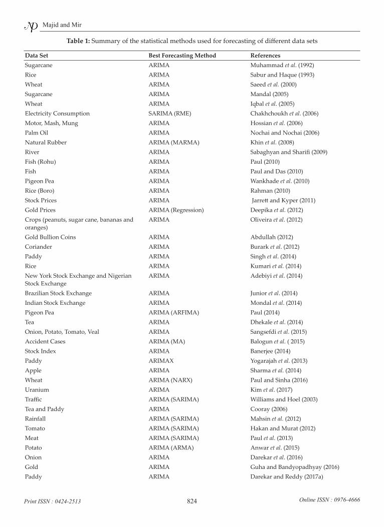
Table 1: Summary of the statistical methods used for forecasting of different data sets

Data Set Best Forecasting Method ReferencesSugarcane ARIMA Muhammad et al. (1992)Rice ARIMA Sabur and Haque (1993)Wheat ARIMA Saeed et al. (2000)Sugarcane ARIMA Mandal (2005)Wheat ARIMA Iqbal et al. (2005)Electricity Consumption SARIMA (RME) Chakhchoukh et al. (2006)Motor, Mash, Mung ARIMA Hossian et al. (2006)Palm Oil ARIMA Nochai and Nochai (2006)Natural Rubber ARIMA (MARMA) Khin et al. (2008)River ARIMA Sabaghyan and Sharifi (2009)Fish (Rohu) ARIMA Paul (2010)Fish ARIMA Paul and Das (2010)Pigeon Pea ARIMA Wankhade et al. (2010)Rice (Boro) ARIMA Rahman (2010)Stock Prices ARIMA Jarrett and Kyper (2011)Gold Prices ARIMA (Regression) Deepika et al. (2012)Crops (peanuts, sugar cane, bananas and oranges)

ARIMA Oliveira et al. (2012)

Gold Bullion Coins ARIMA Abdullah (2012)Coriander ARIMA Burark et al. (2012)Paddy ARIMA Singh et al. (2014)Rice ARIMA Kumari et al. (2014)New York Stock Exchange and Nigerian Stock Exchange

ARIMA Adebiyi et al. (2014)

Brazilian Stock Exchange ARIMA Junior et al. (2014)Indian Stock Exchange ARIMA Mondal et al. (2014)Pigeon Pea ARIMA (ARFIMA) Paul (2014)Tea ARIMA Dhekale et al. (2014)Onion, Potato, Tomato, Veal ARIMA Sangsefdi et al. (2015)Accident Cases ARIMA (MA) Balogun et al. ( 2015)Stock Index ARIMA Banerjee (2014)Paddy ARIMAX Yogarajah et al. (2013)Apple ARIMA Sharma et al. (2014)Wheat ARIMA (NARX) Paul and Sinha (2016)Uranium ARIMA Kim et al. (2017)Traffic ARIMA (SARIMA) Williams and Hoel (2003)Tea and Paddy ARIMA Cooray (2006)Rainfall ARIMA (SARIMA) Mahsin et al. (2012)Tomato ARIMA (SARIMA) Hakan and Murat (2012)Meat ARIMA (SARIMA) Paul et al. (2013)Potato ARIMA (ARMA) Anwar et al. (2015)Onion ARIMA Darekar et al. (2016)Gold ARIMA Guha and Bandyopadhyay (2016)Paddy ARIMA Darekar and Reddy (2017a)



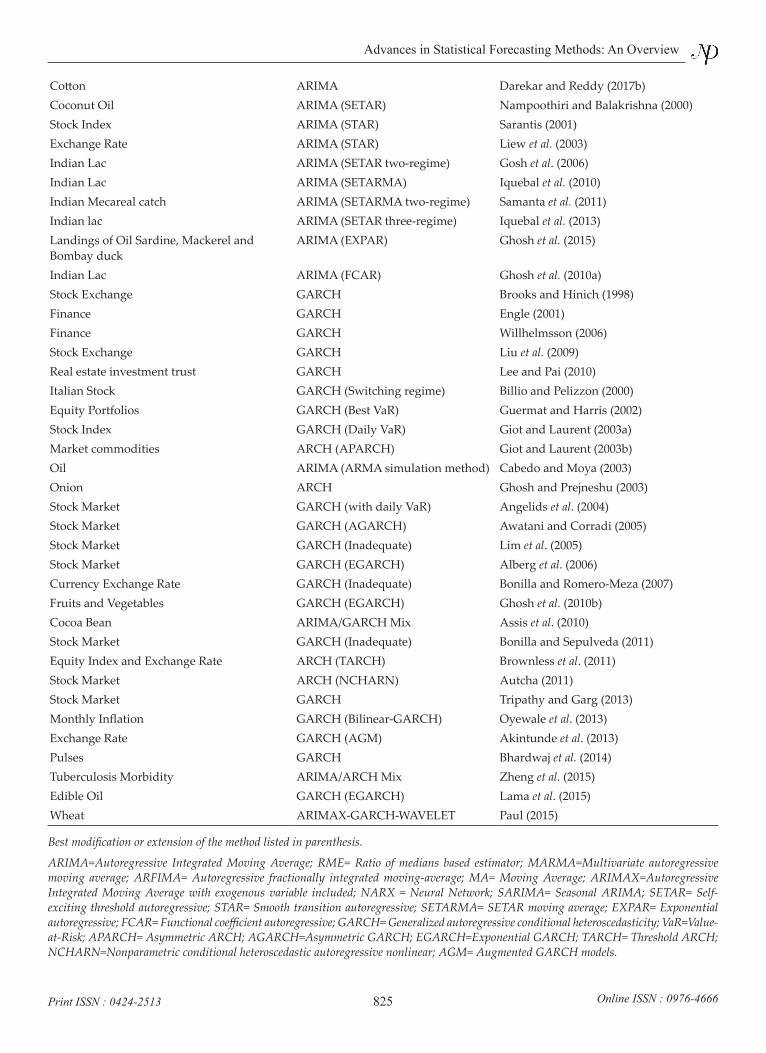
Cotton ARIMA Darekar and Reddy (2017b)Coconut Oil ARIMA (SETAR) Nampoothiri and Balakrishna (2000)Stock Index ARIMA (STAR) Sarantis (2001)Exchange Rate ARIMA (STAR) Liew et al. (2003)Indian Lac ARIMA (SETAR two-regime) Gosh et al. (2006)Indian Lac ARIMA (SETARMA) Iquebal et al. (2010)Indian Mecareal catch ARIMA (SETARMA two-regime) Samanta et al. (2011)Indian lac ARIMA (SETAR three-regime) Iquebal et al. (2013)Landings of Oil Sardine, Mackerel and Bombay duck

ARIMA (EXPAR) Ghosh et al. (2015)

Indian Lac ARIMA (FCAR) Ghosh et al. (2010a)Stock Exchange GARCH Brooks and Hinich (1998)Finance GARCH Engle (2001)Finance GARCH Willhelmsson (2006)Stock Exchange GARCH Liu et al. (2009)Real estate investment trust GARCH Lee and Pai (2010)Italian Stock GARCH (Switching regime) Billio and Pelizzon (2000)Equity Portfolios GARCH (Best VaR) Guermat and Harris (2002)Stock Index GARCH (Daily VaR) Giot and Laurent (2003a)Market commodities ARCH (APARCH) Giot and Laurent (2003b)Oil ARIMA (ARMA simulation method) Cabedo and Moya (2003)Onion ARCH Ghosh and Prejneshu (2003)Stock Market GARCH (with daily VaR) Angelids et al. (2004)Stock Market GARCH (AGARCH) Awatani and Corradi (2005)Stock Market GARCH (Inadequate) Lim et al. (2005)Stock Market GARCH (EGARCH) Alberg et al. (2006)Currency Exchange Rate GARCH (Inadequate) Bonilla and Romero-Meza (2007)Fruits and Vegetables GARCH (EGARCH) Ghosh et al. (2010b)Cocoa Bean ARIMA/GARCH Mix Assis et al. (2010)Stock Market GARCH (Inadequate) Bonilla and Sepulveda (2011)Equity Index and Exchange Rate ARCH (TARCH) Brownless et al. (2011)Stock Market ARCH (NCHARN) Autcha (2011)Stock Market GARCH Tripathy and Garg (2013)Monthly Inflation GARCH (Bilinear-GARCH) Oyewale et al. (2013)Exchange Rate GARCH (AGM) Akintunde et al. (2013)Pulses GARCH Bhardwaj et al. (2014)Tuberculosis Morbidity ARIMA/ARCH Mix Zheng et al. (2015)Edible Oil GARCH (EGARCH) Lama et al. (2015)Wheat ARIMAX-GARCH-WAVELET Paul (2015)

Best modification or extension of the method listed in parenthesis.

ARIMA=Autoregressive Integrated Moving Average; RME= Ratio of medians based estimator; MARMA=Multivariate autoregressive moving average; ARFIMA= Autoregressive fractionally integrated moving-average; MA= Moving Average; ARIMAX=Autoregressive Integrated Moving Average with exogenous variable included; NARX = Neural Network; SARIMA= Seasonal ARIMA; SETAR= Self-exciting threshold autoregressive; STAR= Smooth transition autoregressive; SETARMA= SETAR moving average; EXPAR= Exponential autoregressive; FCAR= Functional coefficient autoregressive; GARCH= Generalized autoregressive conditional heteroscedasticity; VaR=Value-at-Risk; APARCH= Asymmetric ARCH; AGARCH=Asymmetric GARCH; EGARCH=Exponential GARCH; TARCH= Threshold ARCH; NCHARN=Nonparametric conditional heteroscedastic autoregressive nonlinear; AGM= Augmented GARCH models.

Majid and Mir


Beach in Ohio, United States for the period of 2006 to 2008 and compared the performance of various asymmetric models viz EGARCH model, IGARCH model, TGARCH model, GJR-GARCH model, NGARCH model, AVGARCH model and APARCH model and concluded that TGARCH and GJR-GARCH models are better in capturing response of the indicator variable. Akintunde et al. (2013) studied monthly data of exchange rates from Botswana (Pula) and Great Britain (Pound) against United States of America (Dollar) for the period of January 1975 to December 20011 and compared the performance of classical GARCH models with augmented GARCH models and based on minimum variance concluded that Augmented GARCH models (AGM) are more efficient than GARCH models. Bhardwaj et al. (2014) studied spot price data of pulse (Gram) in Delhi market for the period of Fist January 2007 to nineteenth April 2012 and compared the forecasting performance of ARIMA and GARCH models and on the basis of values for RMSE, MSE AND MAPE concluded that in case of volatility, GARCH model is appropriate. Zheng et al. (2015) studied the data of tuberculosis morbidity in Xinjiang, china for the period of January 2004 to June 2014 and compared the performance of ARIMA (1, 1, 2)(1, 1, 1)12 model and ARIMA (1, 1, 2)(1, 1, 1)12 -ARCH(1) model and concluded on the basis of root mean square error (RMSE), mean absolute error (MAE) and mean absolute percentage error (MAPE) that the combined model performs better. Lama et al. (2015) studied three sets of monthly price data viz domestic edibles oils, international edible oils and international raw cotton and applied ARIMA and GARCH models to the data and concluded that for the first two sets AR(2)-GARCH (1, 1) outperformed ARIMA(1, 1, 0) model in terms of forecasting accuracy as directed by low RMSE and RAMPE and in view of the asymmetry of the last set, the EGARCH model was employed in addition to ARIMA and GARCH and found the outperformance of EGARCH over others.There is an innovation called the concept of shrinkage in the process of estimation by the introduction of wavelets. The traditional methodology involves extracting the signal by local smoothing; however such a procedure does not provide useful approximation to the signal when the signal is as or more irregular than the

noise. The signal component can be isolated from the noise component by shrinking the estimates of the wavelet coefficient when the noise is below a threshold and the variation in the signal is above the threshold (Donoho and Johnstone,1995). The statistical properties of wavelet coefficient estimators were derived for the data which is stationary and correlated by Johnstone and Silverman (1997) and for the non-stationary process by VonSachs and MacGibbon (2002). Ghosh et al. (2010c) studied monthly rainfall data of India for the period of 1879-2006 and performed wavelet analysis of the data under frequency domain approach and studied the trend behavior by calculating the discrete wavelet transform (DWT) coefficients and multi resolution analysis (MRA) of the series for Daubechies (D4) and Haar wavelets and based on critical values for both the wavelets concluded the presence of a declining trend. Paul (2015) studied data of annual wheat yield and daily maximum temperature at critical root initiation stage of district Kanpur, Uttar Pradesh, India for the period of 1972-2013 and compared the forecasting performance of ARIMAX model, ARIMAX-GARCH model and ARIMAX-GARCH-WAVELET model and based on Diebold-Mariano test concluded that ARIMAX-GARCH-WAVELET model outperforms the other models.

CONCLUSIONTo evaluate the data for statistical analysis, simple tools and methods were used back in 1950s. The more advanced technology revolutionized the statistical analysis methodologies also as per the analysis requirement for different data sets. The complexity in methods and tools were further enhanced in terms of algorithms, simulations and different parameters based on different data sets. Similarly, the statistical tools for forecasting purposes also evolved with time as per different data sets and analysis requirement. It is also important to note that no single statistical forecasting model is found to be appropriate compared to other methods as evaluated in this review. Thus, there is a need to evaluate the forecasting data using different methods to find the accuracy or near accuracy which in turn depends upon the type of data sets and parameters to evaluate.



REFERENCESAbdullah, L. 2012. ARIMA model for gold bullion coin selling

prices forecasting. International Journal of Advances in Applied Sciences, 1: 153-158.

Abraham, B. and Ledolter, J.1986. Forecast functions implied by autoregressive integrated moving average models and other related forecast procedures. International Statistical Review, 54: 51–66.

Adebiyi, A. A., Adewumi, A.O. and Ayo, C.K. 2014. Stock price prediction using the ARIMA model. 2014 UK Sim-AMSS 16th International Conference on Computer Modelling and Simulation, 15: 105-111.

Akintunde, M.O., Kgosi, P.M. and Shangodoyin, D.K. 2013. Evaluation of GARCH model adequacy in forecasting non-linear economic time series data. Journal of Computations and Modelling, 3(2): 1-20.

Alberg, D., Shalit, H. and Yosef, R. 2006. Estimating stock market volatility using asymmetric GARCH models. http://in.bgu.ac.il/en/humsos/Econ/Working/0610.pdf.

Ali, G. 2013. EGARCH, GJR-GARCH, TGARCH, AVGARCH, NGARCH, IGARCH and APARCH models for pathogens at marine recreational sites. Journal of Statistical and Econometric Methods, 2(3): 57-73.

Angelidis, T., Benos, A. and Degiannakis, S. 2004. The use of GARCH models in VaR estimation. Statistical Methodology, 1: 105–128.

Anwar, M., Shabbir, G., Shahid, M.H. and Samreen, W. 2015. Determinants of potato prices and its forecasting: A case study of Punjab, Pakistan. Munich Personal RePEc Archive No. 66678.

Armstrong, J.S.2001. Principles of Forecasting: A Handbook for Researchers and Practitioners. Springer-233 Spring Street, New York.

Assis, K., Amran, A.and Remali, Y. 2010. Forecasting cocoa bean prices using univariate time series models. Journal of Arts Science & Commerce, 1: 71-80.

Autcha, A. 2011. Developing nonparametric conditional heteroscedastic autoregressive nonlinear model by using maximum likelihood method. Chiang Mai Journal of Science, 38(3): 331-345.

Awartani, A.M.B. and Corradi, V. 2005. Predicting the volatility of the S&P-500 stock index via GARCH models: the role of asymmetries. International Journal of Forecasting, 21: 167-183.

Bachelier, L. 1900. The theory of speculation. Translated by D. May from Annales scientifiques de l’Ecole Normale Superieure, Ser, 3: 21-86.

Baillie, R.T. and Bollerslev, T. 1989. The message in daily exchange rates: A conditional variance tale. Journal of Business and Economic Statistics, 7: 297-305.

Balogun, O.S., Awoeyo, O.O, Akinrefon, A.A. and Yami, A.M. 2015. On the model selection of road accident data in Nigeria: A time series approach. American Journal of Research Communication, 3: 139-177.

Banerjee, D. 2014. Forecasting of Indian stock market using time-series ARIMA model. 2nd International Conference on Business and Information Management, 9-11 Jan.

Bera, A.K. and Higgins, M.L. 1993. ARCH models: properties, estimation and testing. Journal of Economic Surveys, 7: 305-362.

Bhardwaj, S.P., Paul, R.K., Singh, D.R. and Singh, K.N. 2014. An empirical investigation of ARIMA and GARCH models in agricultural price forecasting. Economic Affairs, 59(3): 415-428.

Bianchi, L., Jarrett, J. and Hanumara, T. C. 1998. Improving forecasting for telemarketing centers by ARIMA modeling with interventions. International Journal of Forecasting, 14: 497-504.

Billio, M. and Pelizzon, L. 2000. Value-at-Risk: A multivariate switching regime approach. Journal of Empirical Finance, 7: 531-554.

Boero, G., and Marrocu, E. 2004. The performance of SETAR models: A regime conditional evaluation of point, interval and density forecasts. International Journal of Forecasting, 20: 305- 320.

Bollerslev, T. 1986. A generalized autoregressive conditional Heteroskedasticity. Journal of Econometrics, 31: 307-327.

Bonilla, C.A. and Romero-Meza, R. 2007. GARCH inadequacy for modelling exchange rates: Empirical evidence from Latin America. Applied Economics, pp.1-14.

Bonilla, C.A. and Sepulveda, J. 2011. Stock returns in emerging markets and the use of GARCH models. Applied Economics Letters, 18(14): 1321-1325.

Box, G.E.P. and Jenkins, G.M. 1970. Time series analysis: Forecasting and control, Holden-Day, San Francisco, California, USA.

Box, G.E.P. and Jenkins, G. 1976. Time Series Analysis, Forecasting and Control. Holden- Day, San Francisco.

Box, G.E. P. Jenkins, G.M. Reinsel, G.C. and Ljung, G.M. 2016. Time Series Analysis: Forecasting and Control. Wiley Series in Probability and Statistics, Hoboken, New Jersey.

Brooks, C. & Hinich, M.J. 1998. Episodic non-stationarity in exchange rates. Applied Economics Letters 5: 719-72.

Brooks, C., and Persand, G. 2003. The effect of asymmetries on stock index return value-at-risk estimates. The Journal of Risk Finance, 1: 2348-6848.

Brown, R.G. 1959. Statistical Forecasting for Inventory control, 1st edition, McGRAW-Hill publications.

Brown, R.G. 1963. Smoothing, Forecasting and Prediction of Discrete Time Series. Englewood Cliffs, Prentice-Hall, New Jersey.

Brownless, C., Engle, R. and Kelly, B. 2011. A practical guide to volatility forecasting through calm and storm. The Journal of Risk, 14: 3–22.

Burark, S.S., Sharma, H. and Meena, G.L. 2012. Market integration and price volatility in domestic market of coriander in Rajasthan. Indian Journal of Agricultural Marketing, 27: 121-131.

Majid and Mir


Cabedo, D.J. and Moya, I. 2003. Estimating oil price ’Value at Risk’ using the historical simulation approach. Energy Economics, 25: 239-253.

Chakhchoukh, Y., Panciatici, P. and Mili, L. 2006. Electric load forecasting based on statistical robust methods. IEEE Transactions on Power Systems, 26(3): 982-991.

Chatfield, C., Koehler, A.B., Ord, J.K. and Snyder, R.D. 2001. A new look at models for exponential smoothing. The Statistician, 50: 147–159.

Clements, M.P. and Smith, J. 1997. The performance of alternative methods for SETAR models. International Journal of Forecasting, 13: 463-475.

Cooray, T.M.J.A. 2006. Statistical analysis and forecasting of main agriculture output of Sri Lanka: Rule-based approach. Appeared in 10th International Symposium, Sabaragamuwa University of Sri Lanka, pp 221.

Crouhy, M., Galai, D. and Mark, R. 2000. A comparative analysis of current credit risk models. Journal of Banking & Finance, 24: 59-117.

Darekar, A.S., Pokharkar, V.G. and Yadav, D.B. 2016. Onion price forecasting in Yeola market of Western Maharashtra using ARIMA technique. International Journal of Advanced Biological Research, 6: 551-552.

Darekar, A. and Reddy, A.A. 2017a. Forecasting of common paddy prices in India. Journal of Rice Research, 10: 71-75.

Darekar, A. and Reddy, A.A. 2017b. Cotton price forecasting in major producing states. Economic Affairs, 62: 1-6.

Deepika, M.G., Gautam, N. and Rajkumar, M. 2012. Forecasting price and analyzing factors influencing the price of gold using ARIMA model and multiple regression analysis. International Journal of Research in Management, Economics and Commerce, 2(11): 548-563.

Dhekale, B.S., Sahu, P.K., Vishwajith, K.P., Mishra, P. and Noman, M.D. 2014. Modeling and forecasting of tea production in West Bengal. Journal of Crop and Weed, 10: 94-103.

Donoho, D.L. and Johnstone, I.M. 1995. Adapting to unknown smoothness via wavelet shrinkage. Journal of American Statistical Association, 90: 1200-1224.

Engle, R.F. 1982. Autoregressive conditional heteroscedasticity with estimates of the variance of U.K. inflation, Econometrica, 50: 987-1008.

Engle, R.F. 1983. Estimates of the variance of U.S. inflation based upon the ARCH model. Journal of Money, Credit, and Banking, 15: 286-301.

Engle, R.F. and Kraft, D. 1983. Multi period forecast error variances of inflation estimated from ARCH models, in A. Zellner (ed.), Applied Time Series Analysis of Economic Data (Washington, DC), 293-302.

Engle, R.F., Ito, T. and Lin, W.L. 1990. Meteor showers or heat waves? Heteroskedastic intra-daily volatility in the foreign exchange market. Econometrica, 58: 525-542.

Engle, R. 2001. GARCH 101: The use of ARCH/GARCH models in applied econometrics. Journal of Economic Perspectives, 15: 157-168.

Fildes, R. 1992. The evaluation of extrapolative forecasting methods. International Journal of Forecasting, 8: 81–98.

Franses, P.H., Paap, R. and Vroomen, B. 2004. Forecasting unemployment using an autoregression with censored latent effects parameters. International Journal of Forecasting, 20:255-271.

Franses, P.H. and van Dijk, D. 2005. The forecasting performance of various models for seasonality and nonlinearity for quarterly industrial production. International Journal of Forecasting, 21: 87-102.

French, K.R., Schwert, G.W. and Stambaugh, R.F. 1987. Expected stock returns and volatility, Journal of Financial Economics, 19: 3-10.

Gardner Jr., E. S. 1985. Exponential smoothing: The state of the art. International Journal of Forecasting, 4: 1-38.

Ghosh, H. and Prajneshu. 2003. Non-linear time series modelling of volatile onion price data using AR(p)-ARCH(q)-in-mean. Calcutta Statistical Association Bulletin, 54: 231-247.

Ghosh, H., Sunilkumar, G. and Prajneshu. 2006. Self exciting threshold autoregressive models for describing cyclical data. Calcutta Statistical Association Bulletin, 58: 115-32.

Ghosh, H., Paul, R.K. and Prajneshu 2010a. Functional coefficient autoregressive nonlinear time-series model for forecasting Indian lac export data. Model Assisted Statistics and Applications, 5: 101-108.

Ghosh, H., Paul, R.K. and Prajneshu 2010b. The GARCH and EGARCH nonlinear time-series models for volatile data: An application. Journal of Statistics and Applications, 5: 161-177.

Ghosh, H., Paul, R.K. and Prejneshu. 2010c. Wavelet frequency domain approach for statistical modeling of rainfall time-series data. Journal of Statistical Theory and Practice, 4(4): 812-825.

Ghosh, H., Gurung, B. and Gupta, P. 2015. Fitting EXPAR models through the extended kalman filter. Sankhya: The Indian Journal of Statistics, 77-B: 27-44.

Giot, P. and Laurent, S. 2003a. Market Risk in Commodity Markets: A VaR Approach. Energy Economics, 25: 435-457.

Giot, P. and Laurent, S. 2003b. Value-at-Risk for long and short trading positions. Journal of Applied Econometrics, 18: 641-663.

Glosten, L., Jagannathan, R. and Runkle, D. 1993. On the Relation between Expected Return on Stocks Journal of Finance, 48: 1779–1801.

Granger, C.W.J and Newbold, P. 1986. Forecasting Economic Time Series. Academic Press, Orlando, Florida.

Guermat, C. and Harris, R.D.F. 2002. Forecasting value at risk allowing for time variation in the variance and kurtosis portfolio returns. International Journal of Forecasting, 18: 409-419.

Guha, B. and Bandyopadhyay, G. 2016. Gold price forecasting using ARIMA model. Journal of Advanced Management Science, 4: 117-121.



Hakan, A. and Murat, Y. 2012. An analysis of tomato prices at wholesale level in Turkey: An application of SARIMA model. Custos e @gronegócioon Line, 8: 52-75.

Harvill, J.L. and Ray, B.K. 2005. A note on multi-step forecasting with functional coefficient autoregressive models. International Journal of Forecasting, 21: 717-727.

Holt, C.C. 1957. Forecasting seasonals and trends by exponentially weighted averages (O.N.R. Memorandum No. 52). Carnegie Institute of Technology, Pittsburgh USA.

Holt, C.C. 2004. Forecasting seasonals and trends by exponentially weighted moving averages. International Journal of Forecasting, 20: 5-10.

Hossain, M.Z., Samad, Q.A. and Ali, M.Z. 2006. ARIMA model and forecasting with three types of pulse prices in Bangladesh: A case study. International Journal of Social Economics, 33: 344-353.

Hyndman, R.J. 2001. It’s time to move from what to why. International Journal of Forecasting 17: 567-570.

Hyndman, R.J., Koehler, A.B., Snyder, R.D. and Grose, S. 2002. A state space framework for automatic forecasting using exponential smoothing methods. International Journal of Forecasting, 18: 439–454.

Iqbal, N., Baksh, K., Maqbool, A. and Ahmad, A.S. 2005. Use of the ARIMA model for forecasting wheat area and production in Pakistan. Journal of Agriculture & Social Sciences, 1: 120-122.

Iquebal, M. A., Ghosh, H. and Prajneshu. 2010. Application of genetic algorithm for fitting self-exciting threshold autoregressive nonlinear time-series model. Journal of the Indian Society of Agricultural Statistics, 64: 391-8.

Iquebal, M.A., Ghosh, H. and Prajneshu. 2013. Fitting of SETAR Three-regime nonlinear time series model to Indian lac production data through genetic algorithm .Indian Journal of Agricultural Sciences, 83: 1406-1408.

Jackson, P., Maude, D. J. and Perraudin, W. 1998.Testing Value-at-Risk approaches to capital adequacy. Bank of England Quarterly Bulletin, 38: 256-266.

Jarrett, J.E. and Kyper, E. 2011. ARIMA modeling with intervention to forecast and analyze Chinese stock prices. International Journal of Business and Management, 3: 53-58.

Johnstone, I.M. and Silverman, B.W. 1997. Wavelet threshold estimators for data with correlated noise. Journal of the Royal Statistical Society, 59(2): 319-351.

Junior, P.R., Salomaon, F.L.R and Pamlona, E.O. 2014. ARIMA: An applied time series forecasting model for the Bovespa stock index. Applied Mathematics, 5: 3383-3391.

Kang, I.B. 2003. Multi-period forecasting using different models for different horizons: An application to U.S. economic time series data. International Journal of Forecasting, 19: 387- 400.

Khin, A.A., Eddie, C.F.C, Shamsundin, M.N. and Mohamed, Z.A. 2008. Natural Rubber Price Forecasting in the World Market, Agricultural Sustainability Through Participate Global Extension. University Putra Malaysia, Kuala Lumpur, Malaysia, June 15-19.

Kim, J.H. 2003. Forecasting autoregressive time series with bias corrected parameter estimators. International Journal of Forecasting, 19: 493-502.

Kim, S., Ko, W., Nam, H., Kim, C., Chung, Y. and Bang, S. 2017.Statistical model for forecasting uranium prices to estimatethe nuclear fuel cycle cost. Nuclear Engineering and Technology, 49: 1063-1070.

Kumari, P., Mishra, G.C., Pant, A.K., Shukla, G. and Kujur, S.N. 2014. Autoregressive integrated moving average (ARIMA) approach for prediction of rice (Oryza Sativa L.) yield in India. The Bioscan, 9: 1063-1066.

Lama, A., Jha, G.K., Paul, R.K. and Gurung, B. 2015. Modelling and forecasting of price volatility: an application of GARCH and EGARCH models. Agricultural Economics Research Review, 28 (1): 73-82.

Lambadiaris, G., Papadopoulou, L., Skiadopoulos, G., Zoulis, Y. 2003. VaR: history or simulation? Journal of Risk, 23-26.

Lee, Y.H. and Pai, T.Y. 2010. REIT volatility prediction for skew-GED distribution of the GARCH model. Expert Systems with Applications, 37: 4737-4741.

Liew, V.K.S., Chong, T.T.L. and Lim, K.P. 2003. The inadequacy of linear autoregressive model for real exchange rates: empirical evidences from Asian economies. Applied Economics, 35: 1387- 1392.

Lim, K.P., Hinich, M.J and Liew, V.K.S. 2005. Statistical inadequacy of GARCH models for Asian stock markets: evidence and emplications. Journal of Emerging Market Finance, 4: 263-279.

Liu, H.C., Lee, Y. H. and Lee, M. C. 2009. Forecasting China stock market’s volatility via GARCH models under skewed-GED distribution. Journal of Money, Investment and Banking, 1 (7): 5-15.

Mahsin, M., Akhter, Y. and Begum, M. 2012. Modelling rainfall in Dhaka Division of Bangladesh using time series analysis. Journal of Mathematical Modelling and Application, 1: 67-73.

Makridakis, S. and Hibon, M. 1979. Accuracy of forecasting: An empirical investigation. Journal of the Royal Statistical Society, Series A (General), 142: 97-145.

Makridakis, S., Andersen, A., Carbone, R., Fildes, R., Hibon, M., Lewandowski, R., Newton, J., Parzen, E. and Winkler, R. 1982. The accuracy of extrapolation (time series) methods: Results of a forecasting competition. Journal of Forecasting, 1: 111 – 153.

Mandal, B.N. 2005. Forecasting Sugarcane Productions in India with ARIMA Model. InterStat URL: interstat.statjournals.net/ YEAR/2005/articles/0510002.pdf.

Mandelbrot, B. 1963. New methods in statistical economics. Journal of Political Economy, 71: 421-440.

Mandelbrot, B. 1967. The variation of some other speculative prices. Journal of Business, 40: 393-413.

Masuda, T. and Goldsmith, P.D. 2009. World soybean production: Area harvested, yield and long-term projections. International Food and Agribusiness Management Review, 12: 143-162.

Majid and Mir


Meade, N. 2000. A note on the robust trend and ARARMA methodologies used in the M3 competition. International Journal of Forecasting, 16: 517- 519.

Miller, D. M. and Williams, D. 2003. Shrinkage estimators of time series seasonal factors and their effect on forecasting accuracy. International Journal of Forecasting, 19: 669- 684.

Miller, D. M. and Williams, D. 2004. Damping seasonal factors: Shrinkage estimators for seasonal factors within the X-11seasonal adjustment method (with commentary). International Journal of Forecasting, 20: 529-550.

Mondal, P., Shit, L. and Goswami, S. 2014. Study of effectiveness of time series modeling (ARIMA) in forecasting stock prices. International Journal of Computer Science, Engineering and Applications, 4: 13-29.

Montgomery, D.C. Jennings, C.L. and Kulahci, M. 2008.Introduction to Time Series Analysis and Forecasting, 5th edition, John Wiley & Sons, New Jersey.

Muhammad, F., Javed, M.S. and Bashir, M.1992. Forecasting sugarcane production in Pakistan using ARIMA models. Pakistan Journal of Agricultural Science, 9: 31-36.

Muth, J.F. 1960. Optimal properties of exponentially weighted forecasts. Journal of the American Statistical Association, 55: 299– 306.

Nampoothiri, C.K. and Balakrishna, N. 2000. Threshold autoregressive model for a time series data. Journal of the Indian Society of Agricultural Statistics, 53: 151-160.

Nelson, D.B. 1991. Conditional Heteroskedasticity in asset returns: a new approach. Econometrica, 59: 347-370.

Nelson, D.B. and Cao, C.Q. 1992. Inequality constraints in the univariate GARCH model. Journal of Business and Economic Statistics, 10: 229-235.

Newbold, P., Agiakloglou, C. and Miller, J. 1994. Adventures with ARIMA software. International Journal of Forecasting, 10: 573-581.

Nochai, R. and Nochai, T. 2006. ARIMA model for forecasting oil palm price Proceedings of 2nd IMT-GT Regional Conference on Mathematics, Statistics and Applications, University Sains Malaysia, Penang, 2006.

Oliveira, S. C., Pereira, L. M.M., Hanashiro, J. T. S. and Val, P. C. 2012. A study about the performance of time series models for the analysis of agricultural prices. GEPROS (Gestão da Produção, Operações e Sistemas), 7(3): 11-27.

Oyewale, A.M., Shangodoyin, D.K. and Kgosi, P.M. 2013. Measuring the forecast performance of GARCH and Bilinear-GARCH models in time series data. American Journal of Applied Mathematics, 1(1): 17-23.

Padmanaban, K., Supriya, B.S., Dhekale, B.S. and Sahu, P.K. 2015. Forecasting of tea export from India-An exponential smoothing techniques approach. International Journal of Agriculture Sciences, 7: 577-580.

Pankratz, A. 1991. Forecasting with Dynamic Regression Models. John Wiley & Sons, Inc. New York.

Parzen, E.1982. ARARMA models for time series analysis and forecasting. Journal of Forecasting, 1: 67–82.

Paul, R.K. 2010. Stochastic modeling of wholesale price of rohu in West Bengal, India. Interstat., 11: 1-9.

Paul, R.K. and Das, M.K. 2010. Statistical modelling of inland fish production in India. Journal of the Inland Fisheries Society of India, 42: 1-7.

Paul, R.K., Panwar, S., Sarkar, S.K., Kumar, A., Singh, K.N., Farooqi, S. and Choudhary, V.K. 2013. Modelling and forecasting of meat exports from India. Agricultural Economics Research Review, 26: 249-255.

Paul, R.K. 2014. Forecasting wholesale price of pigeon pea using long memory time-series models. Agricultural Economics Research Review, 27: 167-176.

Paul, R.K. 2015. ARIMAX-GARCH-WAVELET model for forecasting volatile data. Model Assisted Statistics and Applications, 10: 243-252.

Paul, R.K. and Sinha, K. 2016. Forecasting crop yield: A comparative assessment of ARIMAX and NARX model. RASHI, 1: 77-85.

Pegels, C.C. 1969. Exponential smoothing: Some new variations. Management Science, 12: 311-315.

Poon, S. H. and Granger, C.W. J. 2003. Forecasting volatility in financial markets: A review. Journal of Economic Literature, 41: 478-539.

Prejneshu. 2011. Some non-linear time series models and their applications. Journal of the Indian Society of Agricultural Statistics, 66: 243-250.

Quenneville, B., Ladiray, D. and Lefrancois, B. 2003. A note on Musgrave asymmetrical trend-cycle filters. International Journal of Forecasting, 19: 727-734.

Rahman, N.M.F. 2010. Forecasting of boro rice production in Bangladesh: An ARIMA approach. Journal of Bangladesh Agricultural University, 8: 103-112.

Ramasamy, R. and Munisamy, S.2012. Predictive accuracy of GARCH, GJR and EGARCH models select exchange rates application. Global Journal of Management and Business Research, 12(15): 2249-4588.

Reider, R.2009. Volatility Forecasting I: GARCH Models: http://cims.nyu.edu/~almgren/timeseries/Vol_Forecast1.pdf.

Roberts, S.A. 1982. A general class of Holt–Winters type forecasting models. Management Science, 28: 808– 820.

Sabaghyan, J.R. and Sharifi, M.B. 2009. Using stochastic models to simulate and predict the flow of the river by the time series analysis. An international conference on water resources with a regional approach, Tehran, Iran.

Sabur, S.A. and Haque, M.E. 1993.An analysis of rice price in Mymensing town market: Pattern and forecasting. The Bangladesh Journal of Agricultural Economics, 2: 61-75.

Saeed, N., Saeed, A., Zakria, M. and Bajwa, T.M. 2000. Forecasting of wheat production in Pakistan using ARIMA models. International Journal of Agriculture and Biology, 2: 352-353.

Samanta, S., Prajneshu and Ghosh, H. 2011. Modelling and forecasting cyclical fish landings: SETARMA non-linear time series approach. Indian Journal of Fisheries, 58: 39-43.



Sangsefidi, S.J., Moghadasi, R., Yazdani, S. and Nejad, M. 2015. Forecasting the prices of agricultural products in Iran with ARIMA and ARCH models. International journal of Advanced and Applied Sciences, 2: 54-57.

Sarantis, N. 2001. Nonlinearities, cyclical behaviour and predictability in stock markets: International evidence. International Journal of Forecasting, 17: 459-482.

Sentana, E. 1995. Quadratic ARCH models. Review of Economic Studies, 62: 639-61.

Shamiri, A. and Isa, Z. 2009. Modeling and forecasting volatility of the Malaysian stock markets. Journal of Mathematics and Statistics, 5: 234-240.

Sharma, A., Belwal, O.K., Sharma, S.K. and Sharma, S. 2014. Forecasting area and production of apple in Himachal Pradesh using ARIMA model. International Journal of Farm Sciences, 4: 212-224.

Shumway, R.H. and Stoffer, D.S. 2010. Time Series Analysis and its Applications. Springer-233 Spring Street, New York.

Singh, D.P., Kumar, P. and Prabakaran, K. 2013. Application of ARIMA model for forecasting Paddy production in Bastar division of Chhattisgarh. American International Journal of Research in Science, Technology, Engineering & Mathematics, 5: 82-87.

Slutsky, E. 1937. The summation of random causes as the source of cyclic processes. Econometrica, 5: 105-46.

Taylor, S.J. 1986. Modelling Financial Time Series. John Wiley& Sons, Chichester, U.K.

Taylor, J.W. 2003. Exponential smoothing with a damped multiplicative trend. International Journal of Forecasting, 19: 273– 289.

Terasvirta, T. and Anderson, H.M. 1993. Characterizing nonlinearities in business cycles using smooth transition autoregressive models. Journal of Applied Econometrics7: 8119-8136.

Tong, H., Lim, K.S. 1980. Threshold autoregression, limit cycles and cyclical data. Journal of the Royal Statistical Society B., 42: 245-292.

Tripathy, N. and Garg, N. 2013. Forecasting stock market volatility: evidence from six emerging markets. Journal of International Business and Economy, 14(2): 69-93.

Vlaar, P. 2000.Value at Risk models for Dutch bond portfolios. Journal of Banking and Finance, 24: 131-154.

Volterra, V. 1930. Theory of functionals and of integro-differential equations. Dover publications, New York.

VonSachs, R. and MacGibbon, B. 2002. Non-parametric curve estimation by wavelet thresholding with locally stationary errors. Scandinavian Journal of Statistics, 27(3): 475-499.

Wankhade, R., Mahalle, S., Gajbhiye, S. and Bodade, V.M. 2010. Use of the ARIMA model for forecasting pigeon pea production in India. International Review of Business and Finance, 2: 97-102.

Williams, B.M. and Hoel, L.A. 2003. Modeling and forecasting vehicular traffic flow as a seasonal ARIMA process: Theoretical basis and empirical results. Journal of Transportation and Engineering, 129: 664-672.

Willhelmsson, A. 2006. GARCH forecasting performance under different distribution assumptions. Journal of Forecasting, 25: 561-578.

Winters, P.R. 1960. Forecasting sales by exponentially weighted moving averages. Management Science, 6: 324-342.

Wold, H.O. 1938. A Study in the Analysis of Stationary Time Series. Almqvist & Wiksell, Uppsala, Sweden.

Yogarajah, B., Elankumaran, C. and Vigneswaran, R. 2013. Application of ARIMAX model for forecasting paddy production in Trincomalee district in Sri Lanka. Proceedings of the Third International Symposium, SEUSL: 6-7 July 2013, Oluvil, Sri Lanka.

Yule, G.U. 1927. On the method of investigating periodicities in disturbed series, with special reference to Wolfer’s sunspot numbers. Philosophical Transactions of the Royal Society London, Series A., 226: 267- 298.

Zakoian, J. 1994. Threshold heteroskedastic models. Journal of Economic Dynamics and Control, 18: 931-955.

Zheng, Y.L., Zhang, L.P., Zhang, X.L., Wang, K. and Zheng, Y.J. 2015. Forecast model analysis for the morbidity of tuberculosis in Xinjiang, China. PLoS ONE, 10(3): 1-13.

Advances in Statistical Forecasting Methods: An Overview

Documents

Transcript of Advances in Statistical Forecasting Methods: An Overview