ABSTRACT

FREDRICKS, ZACHARY. Quartz Crystal Microbalance Studies of Magnetic Mechanisms

of Atomic-Scale Friction. (Under the supervision of Professor Jacqueline Krim.)

The molecular origins of friction, an important physical phenomenon in light of both

its everyday familiarity and its enormous economic impact, have been discussed and debated

for hundreds of years. The topic has re-emerged and accelerated in recent decades, spurred

by the discovery of wear-free friction mechanisms that arise from both phononic and

electronic phenomena. Magnetic friction, the topic of the present study, has been explored to

a far lesser extent. Recent studies have concluded however that spin dissipation mechanisms

potentially are significant for systems involving magnetic materials. To date, the

experimental studies of magnetic friction have been limited to scanning tip geometries and

passive observations. There have been no experimental demonstrations of magnetic friction

in planar geometries, and no demonstrations of altering friction at the atomic scale by means

of applying an external field.

In this work, I have used a Quartz Crystal Microbalance (QCM) to study nanoscale

friction of magnetic thin films sliding on metals. At temperatures from 30K to 60K, thick and

thin solid and liquid oxygen films were grown on Ni substrates, and their sliding friction

measured in the presence and absence of an applied magnetic field. Sliding of O2 as well as

N2 films on gold electrodes was used as a control.

Friction levels for the oxygen monolayers in the presence of the field were observed

to be reduced significantly compared to those observed in the absence of a field. For thick

films, the reduction was proportionately less, indicating an interfacial effect as the source of

the magnetic sensitivity. The field had no observed effect on the friction levels for the films

of N2 on Au. The results were analyzed in terms of a magnetically-induced adlayer structural

reorientation (magnetostriction) framework as well as the other generally occurring

mechanisms of magnetorheology and spin friction. The observed reduction in friction in the

presence of the magnetic field are consistent with molecular reordering of the adsorbed film

in the presence of the field. Overall, the work constitutes the first definitive demonstration of

magnetically induced changes in friction levels with active control by an external magnetic

field.

© Copyright 2016 by Zachary Fredricks

All rights Reserved

Quartz Crystal Microbalance Studies of Magnetic Mechanisms of Atomic-scale Friction

by

Zachary Fredricks

A dissertation submitted to the Graduate Faculty of

North Carolina State University

in partial fulfillment of the

requirements for the Degree of

Doctor of Philosophy

Physics

Raleigh, North Carolina

2016

APPROVED BY:

____________________________ ____________________________

Daniel Dougherty Kenan Gundogdu

____________________________ ____________________________

Joseph Tracy Jacqueline Krim

Chair of Advisory Committee

ii

DEDICATION

To my mom and to my dad, who always believed in me, even when I doubted myself.

iii

BIOGRAPHY

I was born in Grand Rapids, MI in 1988 and graduated from West Ottawa High

School in 2006. Participation in the Science Olympiad team first ignited my passion for

scientific achievement and we travelled to state and nationals competition. I received a

bachelor’s in physics from Michigan State University in 2011, and subsequently moved to

Raleigh and began graduate study. I attained a master’s degree from NCSU in 2013 and have

enjoyed the experience immensely. Traveling to Italy for a conference as well as presenting

research findings in Baltimore and Long Beach have been recent highlights. Participating in

physics research has been simultaneously humbling and a confidence-building exercise and I

have made many lifelong friends and great memories.

iv

ACKNOWLEDGEMENTS

Foremost I am indebted to Professor Jacqueline Krim, whose utmost dedication and

mentorship has provided many crucial lessons and guidance throughout the years. I couldn’t

imagine a more patient, knowledgeable and inspiring group leader.

I thank committee members Dan Dougherty, Kenan Gundogdu and Joseph Tracy for

their time and useful advice over the course of the program.

Many fruitful discussions were had with professors Robert Riehn, Gerald Lucovsky,

Dave Aspnes, Cheung Ji, and Miroslav Hodak.

The time and energy of fellow past and present group members Zijian Liu, Diana

Berman, Iyam Lynch, Keeley Stevens, Ben Keller, Sam Kenny, Colin Curtis, Steve Corley

and Biplav Acharya is gratefully acknowledged. Ben Hoffman and Andrew Hewitt have

provided help with growing sample films.

Leslie Cochran and Rhonda Bennet have rescued me on several occasions.

To my dear friends Jeff Connell, Gray Williams, Steve Knott and Josh Harris for their

unwavering loyalty.

Thank you to Professors Reinhard Schwienhorst and Wade Fischer, and friends Alex

Rovinski and Amir Ouyed. To my teachers Gus Lukow and Bob Myers for their role in

fostering a culture of excitement for scientific learning for all of us team members - I am

indebted to your efforts.

Steve Galat introduced the word ‘physics’ to my vocabulary as a kid throwing a

Frisbee in the front yard.

To Nick and Ben, and my family, for love and support in the kinetic, adventurous

childhood we shared.

v

TABLE OF CONTENTS

LIST OF TABLES ………………………………………………………………….... vi

LIST OF FIGURES…………………………………………………………………... vii

CHAPTER 1: INTRODUCTION……………………………………………………. 1

CHAPTER 2: REVIEW OF PRIOR WORK ……………………………………… 16

CHAPTER 3: EXPERIMENTAL SETUP………………………………………….. 53

CHAPTER 4: RESULTS AND DISCUSSION OF O2 FILM

GROWTH ON NI AT 47K IN PRESENCE AND ABSENCE OF FIELD………..

88

CHAPTER 5 - RESULTS OF EXPERIMENTS INCREMENTALLY

COOLING O2 FILMS ON NI………………………………………………………...

135

CHAPTER 6: RESULTS OF VARYING APPLIED FIELD ON O2 FILMS IN

EQUILIBRIUM ON AU AND BIPY………………………………………………...

142

CHAPTER 7: RESULTS OF GROWTH OF THIN O2 AND N2 FILMS ON AU

IN PRESENCE VS ABSENCE OF BEXT…………………………………..………

157

CHAPTER 8: CONCLUSIONS……………………………………………………... 165

APPENDIX ………………………………………………………………………….... 172

vi

LIST OF TABLES

Table 4.1. Summary table of O2 films on Ni sliding friction levels at 47.5 K …………...... 110

Table 4.2. Summary table of responses of O2 films on Ni to

magnetic field on/off sequence…………………………………………………………...…

114

Table 4.3. Dissipation channels expected to be open for various

experiments conducted ………………………………………………………………...……

130

Table 6.1. Summary table of O2 thick films grown on Bipy

on Au 2-sided Q sample ………………………………………………………………...…..

156

Table 8.1. Summary of results of applied field on open dissipation channels ………...…... 165

vii

LIST OF FIGURES

Fig. 1.1. Early friction technology ………………………………………………………... 4

Fig. 1.2. Leonardo da Vinci’s studies of friction …………………………………………. 5

Fig. 1.3. Prandtl-Tomlinson model ……………………………………………..………… 9

Fig. 1.4. Macroscopic object on a plane ……………………………………...…………… 10

Fig 1.5. Quartz crystal microbalance schematic …………………………………...……… 12

Fig. 2.1. Presence of magnetic field altering friction …………………………...………… 19

Fig. 2.2. Tip-sample levitation …………………………………………………..………... 20

Fig. 2.3. Monte-carlo of SP-STM …………………………………………...……………. 23

Fig. 2.4. Dissipation of a magnetorheological fluid ………………………...…………….. 24

Fig. 2.5. Chemical vs spin contrast of MEXFM ………………………………..………… 25

Fig. 2.6. Spin degrees of freedom in noncontact force………………………...…………... 26

Fig. 2.7. Spin wave friction ……………………………………………………...………... 28

Fig. 2.8. Magnetic vortex friction ……………………………………………...………….. 30

Fig. 2.9. Effective potential under tip felt by spin …………………………...……………. 31

Fig. 2.10. Variation of steady-state velocity v with force per atom ……………...……….. 33

Fig. 2.11. Adsorption energies along three sliding paths accounting for exchange …...….. 34

Fig. 2.12. Physisorbed O2 on Ni …………………………………………………...……… 37

Fig. 2.13. O2 on Ag(111) ……………………………………………………...…………... 38

Fig. 2.14. O2 on Cu(100) ………………………………………………………...………... 39

Fig. 2.15. Heat flux of o2 on graphite in a field ……………………………………...……. 40

Fig. 2.16. Distribution functions of O2 orientation on graphene ……………………...…... 42

Fig. 2.17. Projections in the plane of simulations of O2 films on graphite ……………..… 44

Fig. 2.18. Simulations of melting of O2 on graphite ………………………..…………….. 45

Fig. 2.19. Dos of majority spin species for O on Ni(111) ………………………...………. 46

Fig. 3.1. Room temperature leak-in calibration ……………………………...…………… 61

Fig. 3.2. Frequency and amplitude shift associated with growth of an O2 thin film …….... 62

Fig. 3.3. Frequency and amplitude measurements are combined

to calculate slip time ……………………………………………………………...………..

63

Fig. 3.4. Effect of introducing 1 Torr O2 to system …………………………………...…... 65

viii

Fig. 3.5. Effect of introducing 7 mTorr O2 to system ………………………………..…… 65

Fig. 3.6. QCM frequency dependence on temperature ………………………………...….. 66

Fig. 3.7. Diagram of UHV cryogenic chamber ………………………………………...…. 70

Fig. 3.8. Picture of UHV cryogenic chamber ………………………………………...…… 71

Fig. 3.9. Picture of the sample cube ……………………………………………..………... 72

Fig. 3.10. Schematic of pierce oscillator circuitry ………………………………..………. 74

Fig. 3.11. Our mixer circuitry ………………………………………………………...…… 75

Fig. 3.12. Picture of experiment control electronics ………………………………..…….. 76

Fig. 3.13. QCM schematic ………………………………………………...………………. 78

Fig. 3.14. Picture of one of my Au QCM samples ……………………………...………… 79

Fig. 3.15. A schematic of the mask ……………………………………………...………... 82

Fig. 3.16. Schematic of flow of data ………………………………………………..…….. 83

Fig. 3.17. Picture of Ni sample fabrication chamber…………………………………...….. 84

Fig. 3.18. Custom LabVIEW program ………………………………………………...….. 85

Fig. 4.1. Calibration of the Ni sample’s resonance amplitude response ………………..… 90

Fig. 4.2.a. Thick O2 film grown on Ni substrate at 47.5K in absence of field ………...….. 91

Figure 4.2.b Thick O2 film grown on Ni substrate at 47.5K in presence of field ……..….. 93

Fig. 4.3. Thick O2 films grown on Ni at 47.5 K in absence of field vs

in presence of field …………………………………………………………..…………….

Fig. 4.4.a. Thin film growth of O2 on Ni in presence of field at 47.5 K……………..……

Fig. 4.4.b. Thin film growth of O2 on Ni in absence of field at 47.5K ……………..…….

94

96

99

Fig. 4.5. Growth of O2 thin film on Ni substrate in presence of B field at 47.5 K ……...… 100

Fig. 4.6. Slip time vs time of a thin O2 film grown on Ni in presence of field ………..….. 101

Fig. 4.7. Slip time vs time of a thin O2 film grown on Ni in absence of field ………...…... 102

Fig. 4.8. Comparison of slip times of two separate thin O2 films grown on Ni

in field present vs field absent ……………………………………………………...……...

103

Fig. 4.9 Effect of a field on average friction levels of thin O2 films

sliding on Ni …………………………………………………………………...…………..

104

Fig. 4.10. Effect of a field on average friction levels of thin O2 films

sliding on Ni for narrow coverage window ………………………………………...……...

105

ix

Fig. 4.11. Slip time vs elapsed time of thick O2 films sliding on Ni in presence vs absence

of field ………………………………………………………………...…………..

106

Fig. 4.12. Comparison of slip times of two separate thick O2 films grown

on Ni in field present vs field absent ………………………………………………...…….

107

Fig. 4.13. Effect of field on averaged friction levels of thick O2 films

sliding on Ni………………………………………………………………………...……...

108

Fig. 4.14. Frequency and inverse quality factor response ………………………...………. 109

Fig. 4.15. The magnet sequence data ………………………………………………..……. 111

Fig. 4.16. The frequency and amplitude data of a thick O2 film ……………………...…... 112

Fig. 4.17. Intermediately thick film ………………………………………………...……... 113

Fig. 4.18. The bulk and 2D phases of molecular oxygen …………………………...…….. 116

Fig. 4.19. Schematic representation of local physical structure of

various phases of 2D O2 ………………………………………………………………...…

117

Fig. 4.20. Molecular orbitals (MO) of oxygen……………………………………………. 118

Fig. 4.21. Illustration of the effect of a magnetic field onto physisorbed O2 films………..

Fig. 4.22. AFM data taken on the Ni sample…………………………………………...….

Fig. 4.23. AFM data taken on an area 500x500 nm…………………………………...…...

122

131

132

Fig. 5.1. Leak in of O2 resulting in a frequency shift ………………………………...….... 136

Fig. 5.2. Amplitude shift due to the introduction of gas ………………………………..… 137

Fig. 5.3. Leak-in of 7 mTorr O2 causing thin film formation …………………………...… 138

Fig. 5.4. Amplitude shift due to the introduction of O2 gas …………………………...….. 138

Fig. 5.5. Temperature dependence of a film’s frequency data ………………………...….. 139

Fig. 5.6. Temperature dependence of a film’s amplitude data ………………………...….. 140

Fig. 5.7. The temperature dependence of O2 thin film friction on Ni

absence of field ………………………………………………………………………….....

141

Fig. 6.1. Calibration of the Bipy/Au-1s-b sample ……………………………………...…. 143

Fig. 6.2. Dosage into sample cell of 7.1 mTorr O2……………………………………...…. 144

Fig. 6.3. Magnetic field with sinusoidal time dependent field strength ………………...… 145

Fig. 6.4. Frequency vs absolute value of applied field ……………………………...…….. 146

Fig. 6.5. Amplitude of oscillation vs absolute value of applied field …………………...… 147

Fig. 6.6. Amplitude of oscillation vs absolute value of applied field of an O2 ………...…. 148

x

Fig. 6.7. At 44 K the field was modulated ……………………………………………..…. 149

Fig. 6.8. Another alternating field applied at temperature setpoint 30k ………………...… 150

Fig. 6.9. Dependence of slip time on coverage for o2 grown on our Bipy-Au/1s ……….... 151

Fig. 6.10. Growth of thick O2 film on Bipy sample in absence of field ………………...… 152

Fig. 6.11. Growth of thick O2 film on Bipy sample in presence of field ………………..... 153

Fig. 6.12. Growth of thick O2 film on Bipy sample in presence of b field ……………..… 154

Fig. 6.13. Frequency shift associated with growing a thick O2 film on Bipy sample …….. 155

Fig. 6.14. Amplitude shift associated with growing a thick O2 film on Bipy sample……... 155

Fig. 7.1. The Au/Au sample is calibrated ………………………………………………..... 157

Fig. 7.2. Compiled data runs of O2 on au film slip time vs coverage …………………..… 158

Fig. 7.3.a Growth of thin N2 film sliding on Au at 47.5 K in presence of field 70g …….... 159

Fig. 7.3.b Growth of thin N2 film sliding on Au at 47.5 K in absence of field ………...…. 160

Fig. 7.4. Control study comparison of thin N2 film on Au at 47.5 K

in absence of field ……………………………………………………………………….....

Fig. 7.5. Compiled data runs of N2 on Au film slip time vs coverage ………………..…...

161

162

1

CHAPTER 1: INTRODUCTION

1.1 Friction and the arrow of time

The macroscopic friction that we are accustomed to observing during everyday life is

a phenomenon emergent primarily from electromagnetic interaction among microscopic

constituents of the system. Friction, in this colloquial sense, is fundamental to all moving

systems we observe. In fact frictional dissipation occurs just as often in systems too small to

observe directly.

Although friction is an inescapable consequence of entropy increase in our universe,

it is not considered a fundamental force in the same sense as gravity, electromagnetism, and

strong and weak nuclear forces. Of these four fundamental forces of nature, friction only

concerns itself with electromagnetism. Gravity is far too weak at this scale, and strong and

weak nuclear forces are too short-ranged. Although there's only one equation governing the

force between two charged particles, the electromagnetic interaction manifests

as friction along varying pathways, which we refer to as 'mechanisms'. For example, in a

stationary frame of reference what may appear as a purely electric field will appear to an

accelerating observer to have a component which is magnetic.

These charge-charge forces can also be represented as van der Waals dipole

interactions. Keesom forces between electric dipole-dipole in polarized molecules, Debye

forces between permanent and induced dipoles, and London dispersion in induced dipole-

induced dipole situations constitute possible modalities. Additionally, magnetic dipole and

exchange interactions are recently being shown to play a role.

An observant student of friction will invariably come across this seeming paradox:

(a) Friction arises solely out of electromagnetic forces.

(b) The force laws governing electrodynamics are reversible in time.

(c) When friction occurs between two objects, it is universally non-reversible.

In this puzzle, (c) does not seem to logically follow from (a) and (b). The trick is the

phenomenological representation of friction as a conversion between organized kinetic

energy into heat or sound. In this total system, energy is not lost – it’s merely converted

(although usable energy is lost).

2

The resolution of this seeming paradox is that microscopic degrees of freedom are

excited, and these tend to be too numerous to count. Instead, through established statistical

mechanics we construct meaningful systemic parameters such as temperature and pressure,

and these don't account for all data within the system but are instead averages. This is the

location within the model at which we 'lose track' of our original energy. From this

enlightened perspective we see that friction isn't a force at all on a fundamental level - it's

instead a statistical happening which concerns the rate of conversion from collective to

individual degrees of freedom - a dissipation process.

Having seen this, the next enlightening feature seems counterintuitive: Dissipation

doesn't scale monotonically with friction. For example, a rigidly attached object cannot be

forced to slide by weak pushing, so there will be no dissipation. As the friction coefficient is

tuned downward, the object will undergo sliding, and a local maximum in dissipation will

occur for a finite value of friction coefficient. This local maximum is necessary from the

viewpoint of considering the opposing limit: that of zero friction. In the zero friction case,

dissipation is also non-existent.

We see that friction concerns itself with degrees of freedom accessible to the system.

In magnetic systems, the spin moment contains energy which depends on orientation and can

thus be considered a degree of freedom akin to the structural lattice excitations. When the

magnetic system is organized into a low-entropy state, or spin polarized, a disturbance can

locally alter the order into a disordered state, stealing energy from the object causing the

disturbance, and this manifests as friction. Likewise if the system has a large disorder

parameter, an ordered body introduced will interact frictionally as its locally introduced order

is dissipated. So the role of magnetism is to provide additional pathways by which friction

can occur. This thesis explores methods by which magnetic frictional mechanisms can be

observed and even controlled at the nanoscale level.

The following chapter is an account of humanity’s continued growth in understanding

and control of frictional processes from the bow-drills of prehistorical use to the friction

force microscopes implemented today.

3

1.2 A history of tribology - from prehistory to today

Although friction is a familiar experience to everyone, its fundamental origins evade

full understanding. Why is liquid water responsible for a nearly negligible sliding coefficient

in the system of an ice skater on a frozen pond, yet a water polo ball is gripped much more

easily when wet? The answer in this case has to do with differences in liquid water behavior

under pressure and friction-induced melting versus the phenomenon of capillary action

increasing surface contact area. Although the material is ideally the same, its behavior

depends on the situation.

One of the first equations taught in elementary physics curricula is:

𝐹𝑓 = 𝜇𝐹𝑁 (1.1)

where μ is friction coefficient and depends on if the object is stationary or sliding with

respect to the plane. Kinetic friction μ𝑘 is generally independent of sliding velocity and is

less than static friction coefficient μ𝑠 for a given material (all else held constant). Upon

introduction to this concept, one would think it possible to predict sliding coefficients, given

any two materials. It’s not so simple in practice - many parameters are at play: temperature,

ambient pressure, contact geometry, sliding speed, load hysteresis, deformation, lubrication,

wear and buildup, moisture, conductivity of materials, roughness, applied fields, etc. This list

is by no means comprehensive - more of a glimpse into the world of tribology - and in fact

the items constitute categories of phenomena each, to which one could devote one’s career.

The field of nanotribology as it exists today seeks to simplify this situation by

focusing on small regions and varying a single parameter at a time in a controlled

environment, and then to compare these systems to find patterns among them. Despite our

best efforts, generally multiple mechanisms are simultaneously present in these studies so

clever ways must be devised if one wishes to make progress in experiments of nanotribology.

The word nanotribology comes from the greek root word “nanos”, meaning dwarf,

implying the 10−9 prefix multiplier and “tribos” meaning “to rub”. Since prehistory,

tribological technology and science have advanced humanity. During the Paleolithic period

105 years ago, humankind took its first steps toward civilized society by mastery of fire

using wood on wood and percussion of flint stones to create sparks. Around 3000-1000 B.C.

in the early civilizations of Mesopotamia, Egypt, China, the Indus Valley and Central and

South America, significant developments occurred. These included thong-drills and bow-

4

drills for boring and fire-making; potter’s wheels used to throw clay vessels; wheeled

vehicles for farming, construction, and warfare; transport of heavy stones using sledges; and

lubricating materials (water, oil, and beef tallow) [1].

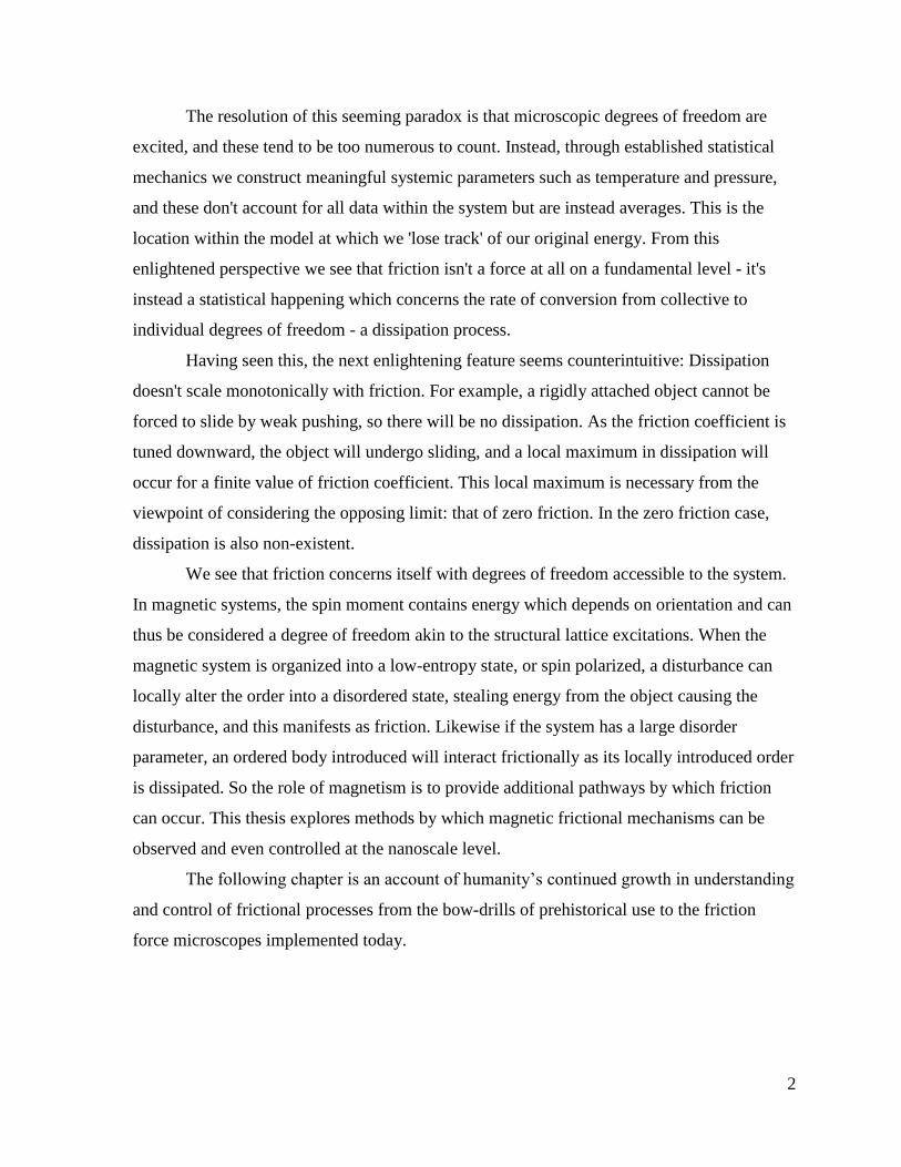
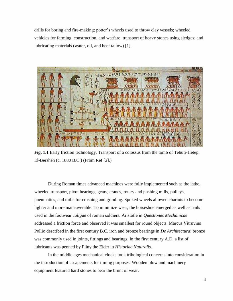
Fig. 1.1 Early friction technology. Transport of a colossus from the tomb of Tehuti-Hetep,

El-Bersheh (c. 1880 B.C.) (From Ref [2].)

During Roman times advanced machines were fully implemented such as the lathe,

wheeled transport, pivot bearings, gears, cranes, rotary and pushing mills, pulleys,

pneumatics, and mills for crushing and grinding. Spoked wheels allowed chariots to become

lighter and more maneuverable. To minimize wear, the horseshoe emerged as well as nails

used in the footwear caligae of roman soldiers. Aristotle in Questiones Mechanicae

addressed a friction force and observed it was smallest for round objects. Marcus Vitruvius

Pollio described in the first century B.C. iron and bronze bearings in De Architectura; bronze

was commonly used in joints, fittings and bearings. In the first century A.D. a list of

lubricants was penned by Pliny the Elder in Historiae Naturalis.

In the middle ages mechanical clocks took tribological concerns into consideration in

the introduction of escapements for timing purposes. Wooden plow and machinery

equipment featured hard stones to bear the brunt of wear.

5

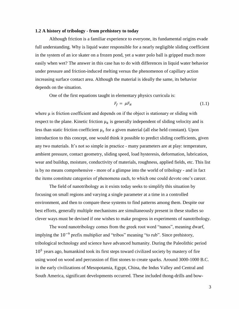
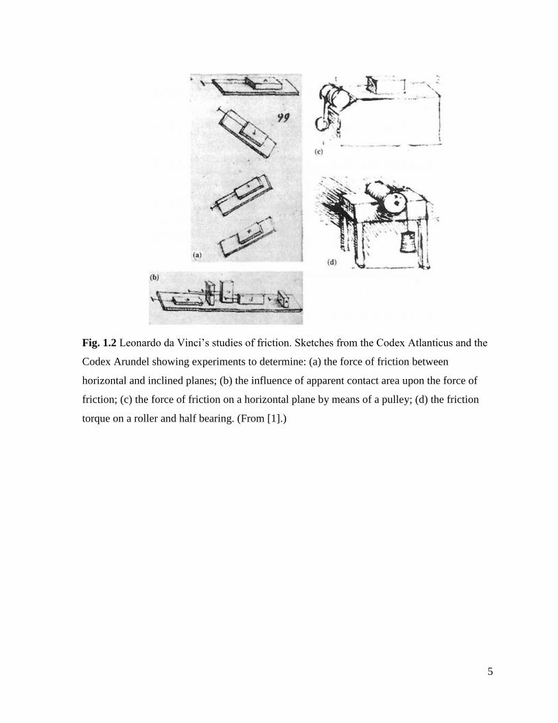
Fig. 1.2 Leonardo da Vinci’s studies of friction. Sketches from the Codex Atlanticus and the

Codex Arundel showing experiments to determine: (a) the force of friction between

horizontal and inclined planes; (b) the influence of apparent contact area upon the force of

friction; (c) the force of friction on a horizontal plane by means of a pulley; (d) the friction

torque on a roller and half bearing. (From [1].)

6

During the Renaissance period Leonardo da Vinci conducted the first scientific

studies of friction and recorded these in Codex Madrid I and Codex Atlanticus. He

discovered the first two laws of friction, which are attributed to Amontons, and specified a

low-friction bearing alloy: “mirror metal” of tin and copper. Steel alloys were employed, and

an emerging machinery scene recognized the importance of tribology.

Prior to the Industrial Revolution an explosion of interest in tribology occurred;

scientists began publishing in books their theories and experiments. Guillaume Amontons

conducted sliding friction experiments and in 1699 reported three laws of friction, which

were later verified by Coulomb:

1. Frictional force is directly proportional to applied load

2. Frictional force is independent of apparent area of contact

3. Kinetic friction is independent of sliding velocity

In 1687 in Principia Newton gave a law of viscous friction:

𝑠ℎ𝑒𝑎𝑟 = 𝜇

𝜕𝑢

𝜕𝑦

(1.2)

which to this day lays the basis for our modern understanding of viscous fluid flow. 𝑠ℎ𝑒𝑎𝑟 is

shear stress, μ dynamic viscosity, u fluid speed, and y distance from the interface. Leibnitz

published work in 1706 distinguishing between rolling and sliding friction. Leonhard Euler’s

1750 publications introduced μ as friction coefficient and distinguished between static and

kinetic friction. During this time bearing materials were considered and experimented with;

Brass and bronze bearings were commonly implemented. The roller bearing concept was

experimented upon and lessened wear and need for motive power. Desaguliers in 1734

tabulated coefficients of friction for various materials and suggested that lubricant acted as

tiny rollers and filled imperfections in the interface.

The emergence of the steam engine and railways in the early 1800s was both

influenced by and demanded improvements in tribology. This shift caused massive changes

in agriculture, transportation of goods and people, and industry. It lead to efforts in training

and educating engineers and scientists, leading further to the formation of scientific societies.

Practical problems such as coin wear, wheel-rail adhesion, and rope stiffness on pulleys

motivated in-depth experimentation and study, advancing the field of tribology.

7

The Navier-Stokes equation governing fluid friction developed in 1823 was applied

to liquid lubrication later in the century. Poiseuille in 1846 experimented with viscous flow

in pipes to better understand blood flow in capillaries.

Mineral oils came to increasingly greater usage as well as sperm oil, whale oil, rape-

seed oil, olive oil, lard oil, fish oils, and solid lubricants graphite and talc, and specifications

of their mixtures found for increased lubrication of various components of machinery.

Patents came about for lubricant mixtures and their extraction methods, as well as for friction

wheels and rolling element bearings.

The rise of oil companies Socony, Exxon, Socal, Texaco, British Petroleum and

others in the late 1800s and early 1900s marked a change in usage from vegetable and animal

oils and fats to mineral oils as lubricants. This prompted research around the world in thin

film lubrication. Gustav-Adolphe Hirn in the 1840s developed a friction balance for studies

of friction of bronze bearings dipped in lubricant. He found a first order velocity dependence

for lubricated coefficient of friction at constant temperature and demonstrated the usefulness

of mineral oil as a lubricant. Robert Henry Thurston in 1879 was the first to report that

coefficient of friction undergoes a minimum upon transition from increased loading and

increased speed from fluid film to boundary lubrication. Richard Stribeck systematized

journal friction experiments in the 1890s, revealing a curve consistent with the minimum

recognized by Thurston.

Beauchamp Tower in 1883 discovered through journal friction experiments that very

large pressures were generated in the lubricant in journal bearings and also that the lubricated

case followed liquid friction laws. These discoveries suggested for future studies the

importance of hydrodynamic analysis as well as a redesign of lubricant application devices.

Osbourne Reynolds contributed greatly in theoretical analysis including equations of

fluid-film lubrication and micro-slip in rolling friction and provided keen insight into the

cavitation of lubricant films as well as insights into slipping friction between mechanical

elements. Petrov in the 1880s in applying Newton’s viscosity relation to hydrodynamic

analysis of lubricant between sliding concentric cylinders found a relation – today known as

Petrov’s Law - for friction of lubricating films at the interface of sliding journal bearings.

In 1918 Lord Rayleigh applied the experimental finding of surface tension of water

changing upon introduction of thin oil film to the sliding of solid bodies, showing these

8

monolayer films to be responsible for greatly decreasing the friction. A distinction was now

growing between ‘boundary lubrication’, in which a thin oily film was present, and complete

lubrication, in which the friction was governed by liquid laws. This distinction was advanced

by Hardy and Doubleday in 1922 in their experiments with thin films of oils of varying

molecular weight, showing a negative dependence of friction with increased molecular

weight (and thus chain length). Mayo D. Hersey was the first to use dimensional analysis to

show the friction obeyed a unique function of:

𝜂𝑣

𝑝 (1.3)

where η is viscosity, v is speed, and p is pressure in journal bearings. Ball bearings originally

being made of cast iron required high contact stresses and thus required special steels,

prompting further research and various patented designs.

The 20th century marked a shift in understanding that frictional behavior was

dominated in many cases by molecular interactions at the interface. There had always been

great dispute as to even the existence of molecules, but with seminal work such as van der

Waals’ on molecular sizes and forces and Einstein’s 1905 papers on Brownian motion it was

becoming evident that molecular structure effects could be observed. The Prandtl-Tomlinson

model, originating from two papers in 1928-1929 explains how a velocity-independent

friction force arises from a sliding tip on a substrate [3].

9

Fig 1.3. Prandtl-Tomlinson model. (a) A massive block slides with constant speed, dragging

a tip via a spring across a periodic potential landscape. (b) Accounting for finite temperature

slip events. (From [3].)

This model, commonly used by nanotribologists to this day, involves a tip, which is

attached by a spring to a mass sliding with constant velocity, interacting with a substrate

corrugation energy landscape as well as velocity-dependent damping. Interactions are shown

to undergo stick-slip to sliding behavior as system parameters spring constant, corrugation

amplitude and sliding speed are varied. Since its inception, the model has been modified for a

given body and expanded to include multiple masses, such as in the Frenkel-Kontorova

model in 1938 [4].

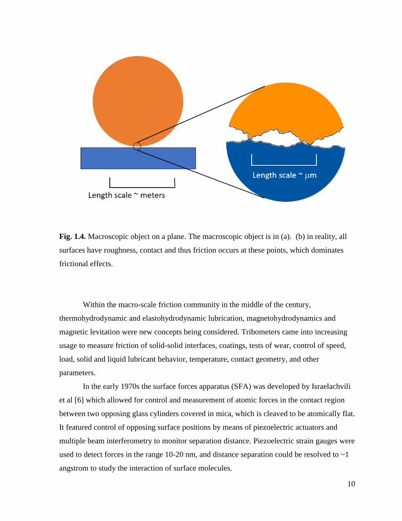
Bowden and Tabor in 1940-1954 when analyzing single asperity contact deformation

revealed the reason that sliding friction coefficient is independent of apparent contact area:

All surfaces have some variation in their height profile, of which root-mean-square

roughness parameter, asperity radius of curvature and fractal dimension are common ways to

characterize. Upon the meeting of two surfaces, contact occurs at the peaks first, and as the

materials are pushed together deformation occurs (plastic or elastic) in regions of real contact

areas, whose size is dependent upon load, and it is at these real contact regions where friction

occurs [5].

10

Fig. 1.4. Macroscopic object on a plane. The macroscopic object is in (a). (b) in reality, all

surfaces have roughness, contact and thus friction occurs at these points, which dominates

frictional effects.

Within the macro-scale friction community in the middle of the century,

thermohydrodynamic and elastohydrodynamic lubrication, magnetohydrodynamics and

magnetic levitation were new concepts being considered. Tribometers came into increasing

usage to measure friction of solid-solid interfaces, coatings, tests of wear, control of speed,

load, solid and liquid lubricant behavior, temperature, contact geometry, and other

parameters.

In the early 1970s the surface forces apparatus (SFA) was developed by Israelachvili

et al [6] which allowed for control and measurement of atomic forces in the contact region

between two opposing glass cylinders covered in mica, which is cleaved to be atomically flat.

It featured control of opposing surface positions by means of piezoelectric actuators and

multiple beam interferometry to monitor separation distance. Piezoelectric strain gauges were

used to detect forces in the range 10-20 nm, and distance separation could be resolved to ~1

angstrom to study the interaction of surface molecules.

11

Atomic resolution became possible in 1981 with the development of scanning

tunneling microscopy (STM) by Gerd Binnig and Heinrich Rohrer [7]. A sharp metal tip,

held at bias voltage, is scanned over the surface controlled by piezoelectric actuators,

measuring the work function of tunneled electrons. A control loop is present which causes

the tunneling current to be constant by altering the tip-substrate distance. Soon similar

techniques were developed: atomic force microscopy (AFM) and friction force microscopy

(FFM) measuring respectively deflection of a light ray by the cantilever and the twisting

mode feedback of the cantilever. These techniques allow to measure sub-nanoNewton forces

occurring between single asperities and substrates in various environments: ultrahigh vacuum

(UHV), ambient air, controlled atmosphere, or liquid environments.

A new nanoscale frictional measurement technique was pioneered in 1988 by Krim

and Widom [8] utilizing a quartz crystal microbalance (QCM), a tool that had hitherto been

used primarily as a mass uptake sensor as well as timing devices. The dissipation of the

oscillator is monitored alongside its frequency in a controlled environment to determine

interfacial friction levels occurring between the electrode and an adsorbed film. Since the

introduction of the technique it has been used to study many frictional behaviors including

sliding film and pinning behavior of noble gases on metal substrates, physisorbed films,

spreading diffusion, fullerenes and molecular lubricants, superconducting transitions, and

dissipation in aqueous environments [12].

12

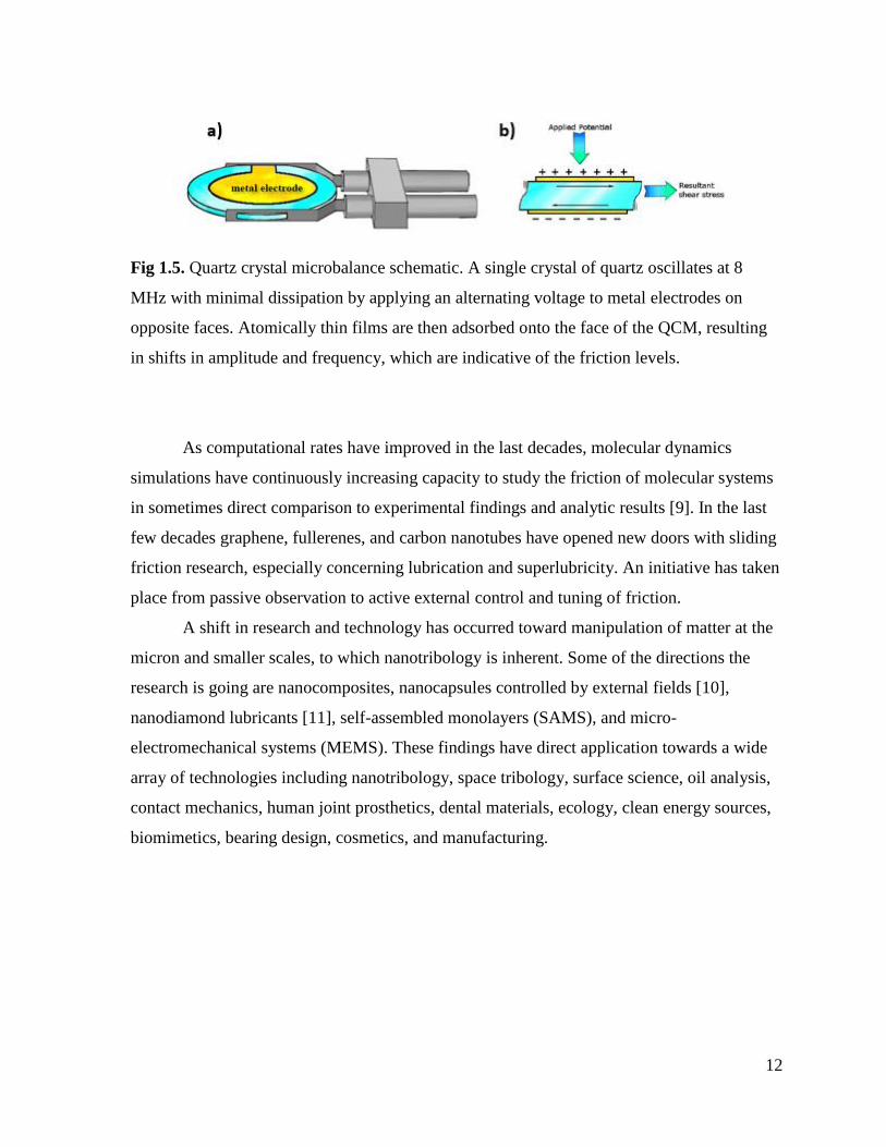
Fig 1.5. Quartz crystal microbalance schematic. A single crystal of quartz oscillates at 8

MHz with minimal dissipation by applying an alternating voltage to metal electrodes on

opposite faces. Atomically thin films are then adsorbed onto the face of the QCM, resulting

in shifts in amplitude and frequency, which are indicative of the friction levels.

As computational rates have improved in the last decades, molecular dynamics

simulations have continuously increasing capacity to study the friction of molecular systems

in sometimes direct comparison to experimental findings and analytic results [9]. In the last

few decades graphene, fullerenes, and carbon nanotubes have opened new doors with sliding

friction research, especially concerning lubrication and superlubricity. An initiative has taken

place from passive observation to active external control and tuning of friction.

A shift in research and technology has occurred toward manipulation of matter at the

micron and smaller scales, to which nanotribology is inherent. Some of the directions the

research is going are nanocomposites, nanocapsules controlled by external fields [10],

nanodiamond lubricants [11], self-assembled monolayers (SAMS), and micro-

electromechanical systems (MEMS). These findings have direct application towards a wide

array of technologies including nanotribology, space tribology, surface science, oil analysis,

contact mechanics, human joint prosthetics, dental materials, ecology, clean energy sources,

biomimetics, bearing design, cosmetics, and manufacturing.

13

1.3 Aim of this thesis

In existing literature, there is agreement that frictional behavior depends on which

dissipation channels are open to the system – phononic, electrostatic, and electronic

mechanisms are well-established [12]. Magnetic degrees of freedom have been shown

experimentally and in theory and in simulation to play a role in the dissipation processes

taking place at various interface geometries and materials. These phenomena include

magnetorheology, magnetostriction, spin friction, and magnons; however, to date, no sliding

friction experiments have been conducted on a nanoscale film-substrate system with

magnetic properties to elucidate which channels exist for a given system. The primary aim of

this thesis is to conduct QCM friction experiments on systems of various known magnetic

properties, so that the means of dissipation can be understood by comparing results across the

various systems.

In chapter 2, we elaborate on the recent efforts in atomic-scale friction research of

magnetic systems, as well as systems whose frictional levels are otherwise dependent upon

an applied magnetic field. Chapter 3 elaborates on the experimental details of the device I

designed and constructed which measures frictional behavior in nanoscale thin film-substrate

systems which are paramagnetic, ferromagnetic, antiferromagnetic, and diamagnetic in

nature, as well as detailing the data-taking procedure using this system. In Chapter 4 and 5 I

discuss the results of the studies, and concluding remarks are issued in Chapter 6.

14

REFERENCES CHAPTER 1

[1] Dowson, D. (1979). History of Tribology. New York: Longman Group Limited.

[2] Fall, a., Weber, B., Pakpour, M., Lenoir, N., Shahidzadeh, N., Fiscina, J., … Bonn, D.

(2014). Sliding friction on wet and dry sand. Physical Review Letters, 112(May), 3–6.

http://doi.org/10.1103/PhysRevLett.112.175502

[3] Schwarz, U. D., & Hölscher, H. (2016). Exploring and Explaining Friction with the

Prandtl-Tomlinson Model. Acs Nano, 10, 38–41. http://doi.org/10.1021/acsnano.5b08251

[4] Braun, O. M., & Kivshar, Y. S. (1998). Nonlinear dynamics of the Frenkel — Kontorova

model. Physics Reports, 306, 1–108. http://doi.org/10.1016/s0370-1573(98)00029-5

[5] Bowden, F. P., & Tabor, D. (1950). The Friction and Lubrication of Solids. London:

Oxford at the Clarendon Press.

[6] Israelachvili, J. N., & Adams, G. E. (1976). Direct measurement of long range forces

between two mica surfaces in aqueous KNO3 solutions. Nature, 262, 774–776.

http://doi.org/10.1038/262774a0

[7] Binnig, G., Rohrer, H., Gerber, C., & Weibel, E. (1982). Surface studies by scanning

tunneling microscopy. Physical Review Letters, 49(1), 57–61.

http://doi.org/10.1103/PhysRevLett.49.57

[8] Widom, A., & Krim, J. (1988). Damping of a crystal oscillator by an adsorbed monolayer

and its relation to interfacial viscosity. Physical Review B, 38(17), 184–189.

[9] Cieplak, M., Smith, E. D., & Robbins, M. (1994). Molecular Origins of Friction : The

Force on Adsorbed Layers, 265(5176), 1209–1212.

[10] Tietze, R., Zaloga, J., Unterweger, H., Lyer, S., Friedrich, R. P., Janko, C., Alexiou, C.

(2015). Magnetic nanoparticle-based drug delivery for cancer therapy. Biochemical and

Biophysical Research Communications, 468(3), 463–470.

http://doi.org/10.1016/j.bbrc.2015.08.022

15

[11] Liu, Z., Leininger, D., Koolivand, a., Smirnov, a. I., Shenderova, O., Brenner, D. W., &

Krim, J. (2015). Tribological properties of nanodiamonds in aqueous suspensions: Effect of

the surface charge. RSC Advances, 5, 78933–78940. http://doi.org/10.1039/c5ra14151f

[12] Krim, J. (2012). Friction and energy dissipation mechanisms in adsorbed molecules and

molecularly thin films. Advances in Physics, 61(December), 155–323.

http://doi.org/10.1080/00018732.2012.706401

16

CHAPTER 2: REVIEW OF PRIOR WORK

Since nanotribology has blossomed in the last decades, it has sprawled into

neighboring fields of research: physics, chemistry, and materials science. Additionally the

individual mechanisms of dissipation at an interface have received attention. Phononic

mechanisms are generally dominant and contribute when molecular or atomic vibrations are

excited at an interface. The subsequent damping that occurs dissipates energy throughout the

system, which is measured as friction. Theory and experiment have documented nanoscale

phononic mechanisms, for example in the case of monolayer films sliding on a substrate

[1,2]. When a conducting material is in the vicinity of the interface, any lateral sliding that

takes place can drag electrons along inside of the material. These charge carriers then scatter

from defects in the material, thus dissipating energy through ohmic losses. These types of

interactions are categorized under the conduction electronic mechanisms of nanoscale

friction.

When a material at the interface or part of it is insulating, electrons can become

trapped, resulting in an electrostatic force between it and the other elements of the geometry.

Sliding friction will then be affected by this electrostatic mechanism. AFM research has been

done recently which isolates electronic mechanisms, although the results are not well agreed-

upon.

In addition to these, magnetic mechanisms have been shown to be prominent in

situations involving magnetic materials. For multiple scenarios and geometries, a change in

friction is theorized [3-7] and experimentally shown [8-10] when a field is present. By

studying frictional forces in different scenarios, one can isolate and observe effects of

magnetism on friction.

Although experimental observation is possible, the field does face challenges which

current research attempts to address. The order of magnitude of the strength of these

magnetic frictional interactions is not well agreed upon, but is currently being explored.

Typical devices that have been used for atomic friction are the quartz crystal microbalance

(QCM), surface forces apparatus (SFA), AFM and STM. Of these devices, none have in-built

capability of resolving atomic-scale magnetic behavior. However, the traditional methods can

be altered in certain setups to be receptive to nanoscale magnetic phenomena. Also, some

17

new techniques have been invented, such as magnetic force microscopy (MFM) and spin-

polarized scanning tunneling microscopy (SP-STM). Today it is established phononic,

electronic, electrostatic and magnetic degrees of freedom play their role. This chapter focuses

on how recent studies of magnetic degrees of freedom have been observed to play a role in

nanofriction, and how united picture is beginning to emerge.

Typical of these studies are established techniques: quartz crystal microbalance

(QCM), magnetic force microscopy (MFM), magnetic exchange force microscopy (MexFM),

spin-polarized scanning-tunneling microscopy (SP-STM), density functional theory (DFT),

and molecular dynamics simulations (MD). QCM studies are used with a either a magnetic

metal electrode material, or a magnetic adsorbate material; a superconductive material;

electromagnetic field generation or permanent magnets. MFM and MexFM studies have used

an AFM tip coated in a magnetized material, in at least one case in conjunction with a

superconducting substrate and SP-STM involves a similar idea with a magnetized scanning-

tunneling microscope tip.

18

2.1. Prior Experimental Studies

The existing literature concerning experimental studies of magnetic friction falls into

several categories. This section is divided into studies in which magnets were used and

studies in which magnetic effects were observed (the latter being inclusive of magnets being

used).

2.2. Studies utilizing magnetic fields

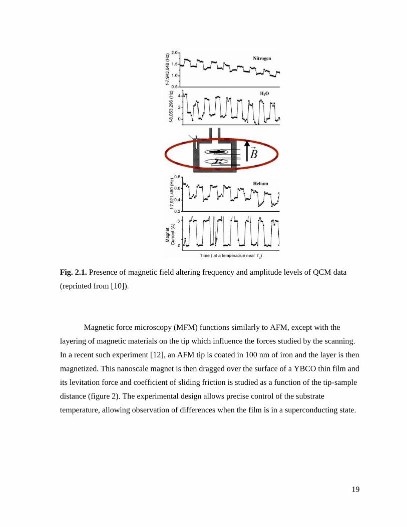
The quartz crystal microbalance (QCM) technique has been implemented continually

by the Krim group and the Mistura group. Quartz, a dielectric material, can be cut into a

small disc and set into megahertz shear oscillation by means of a periodic applied potential.

Measurement of nanoscale friction is possible at the interface of the oscillator electrode and

the adsorbed film by recording of the amplitude and frequency of oscillation. In an

experimental study [10], a 200 nm Pb film was deposited atop the bare quartz. The sample

was then cooled and a film of either He, N2 or H2O was deposited onto the surface, after

which the sample was warmed. This heating brought the sample through the superconducting

threshold temperature of Pb.

As this gradual heating took place, a magnetic field was applied periodically which

brought the substrate Pb into and out of the superconducting state (Figure 5). The frequency

of oscillation of the QCM was responsive to this change in magnetic state, indicating an

increase in dissipation when the substrate was no longer superconducting. The sliding

friction was increased by a factor of 10-20. The measured values of friction coefficients

agreed well with earlier observations and theory [11] of electronic mechanisms of friction.

This work elucidates the temperature dependence of friction of a widely studied

superconductor, and the results will be applicable whenever it is used at an interface. This

study ties into magnetic friction to the extent that superconductivity is controlled by a field.

19

Fig. 2.1. Presence of magnetic field altering frequency and amplitude levels of QCM data

(reprinted from [10]).

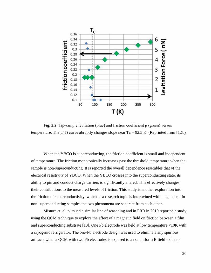
Magnetic force microscopy (MFM) functions similarly to AFM, except with the

layering of magnetic materials on the tip which influence the forces studied by the scanning.

In a recent such experiment [12], an AFM tip is coated in 100 nm of iron and the layer is then

magnetized. This nanoscale magnet is then dragged over the surface of a YBCO thin film and

its levitation force and coefficient of sliding friction is studied as a function of the tip-sample

distance (figure 2). The experimental design allows precise control of the substrate

temperature, allowing observation of differences when the film is in a superconducting state.

20

Fig. 2.2. Tip-sample levitation (blue) and friction coefficient μ (green) versus

temperature. The μ(T) curve abruptly changes slope near Tc = 92.5 K. (Reprinted from [12].)

When the YBCO is superconducting, the friction coefficient is small and independent

of temperature. The friction monotonically increases past the threshold temperature when the

sample is non-superconducting. It is reported the overall dependence resembles that of the

electrical resistivity of YBCO. When the YBCO crosses into the superconducting state, its

ability to pin and conduct charge carriers is significantly altered. This effectively changes

their contributions to the measured levels of friction. This study is another exploration into

the friction of superconductivity, which as a research topic is intertwined with magnetism. In

non-superconducting samples the two phenomena are separate from each other.

Mistura et. al. pursued a similar line of reasoning and in PRB in 2010 reported a study

using the QCM technique to explore the effect of a magnetic field on friction between a film

and superconducting substrate [13]. One Pb electrode was held at low temperature <10K with

a cryogenic refrigerator. The one-Pb electrode design was used to eliminate any spurious

artifacts when a QCM with two Pb electrodes is exposed to a nonuniform B field – due to

21

differences in relative position of the electrodes with respect to the magnet. As well, some

artifacts in the QCM response at low temperature were taken note of by the authors.

In the experiment, two Meissner coils were used to detect magnetic flux expulsion of

the films to determine superconducting state. As well, a manipulator wheel with an attached

permanent magnet was used to force the Pb into and out of the superconducting state. A film

was condensed onto the face of the QCM by exposure to low vapor pressure Ne gas. The

frequency and amplitude of the resonators were used with the frequency modulation

technique about the resonant frequency.

For the bare QCMs, the crossing of the thermal transition was not signaled by any

change in frequency or amplitude, as was observed with a QCM with two electrodes – this

was attributed to a larger series resistance of the one-Pb electrode design (presumably

provided by the Au electrode). When the Pb electrode is in the superconducting phase, the

frequency and amplitude can be changed by introducing a permanent magnet, even if the

state remains superconducting. Also, by using the magnet to cross into the non-

superconducting state, the frequency was lowered. As well, at variance with what was

reported in the earlier study [14] no increase in frequency was observed with increasing the

system temperature through the superconducting transition, although a difference in

amplitude was observed.

The explanation the authors provide is that a thermal annealing is required to 50-60K

in order to make the oscillation responses highly reproducible. This annealing requirement

was thought to clear the QCM of mechanical stresses before running the experiment. This

thermal cycle was found also to be required to detect any slippage of the adsorbate gas upon

film growth. It was thenceforth left unclear whether this annealing procedure was specific to

their design, or would be required for reproducibility in general for low temperature QCM

studies.

22

2.3 Magnetic frictional mechanisms are observed

Another method for measurement of magnetic friction is spin-polarized scanning

tunneling microscopy (SP-STM) [9]. It is a similar technique to AFM, except the tip has been

coated in a magnetic material. Recent experiments and simulations by Wolter et al and

Wiesendanger et al [15] have elucidated effects the spin degree of freedom has on friction

using this technique. The potential caused by the SP-STM tip was used to trap and then

control the movement of individual Co atoms over the surface of Mn/W(110). The behavior

of the Co atom is reflective of the magnetic order of the substrate.

As the tip moves laterally, the dragged Co atom shows increased energy within one

site on the surface, and subsequently abrupt hopping takes place between sites, during which

energy is dissipated. When the tip is magnetically unpolarized, the energy of hopping is

independent of local spin state in the substrate. When the tip is magnetized, the energy is no

longer degenerate; the atom prefers sites whose electron spins are parallel to the tip (Figure

2.3). The measurement of this subtle energy behavior allows derivation of the lateral forces

~10-10 N which are in good agreement with experiment. It requires only about half the force

to move the adsorbed atom from an antiparallel site to a parallel site, than in the opposite

direction.

This work has generated an abundance of effort in the simulation community as well

as in experiments with aim to understand the underlying dissipation mechanisms. Also,

because the tip field is localized, it has put forth the question of a 2D magnetic system’s

behavior. In a localized field, such as the tip’s, the gradients are large, and ultimately it is the

magnetic field gradient which is responsible for spin flip and electronic processes.

23

Fig.2.3. Setup and results of Monte Carlo simulations (a) Top view of the equilibrium

adsorption sites of the Co adatom (blue). (b) Side view of the Monte Carlo simulation setup.

(c) Top view (dashed arrows indicate tip path), side view of the adatom position (dotted

orange line indicates average adatom height of the nonmagnetic case), and [110] component

(up or down) of the adatom spin during manipulation, for different strengths of the tip-

adatom exchange interaction Jtip, sampled at constant time intervals. (d) Adatom energy and

(c) lateral force as a function of tip position, for the three cases presented in (c). The black

arrows indicate the spin configuration of the tip and adsorption site. (Reprinted from [9].)

Thus far, we have explored QCM studies in which a field was used to probe friction.

In an experimental concept in parallel with the line of questioning of this thesis, a study has

been reported within the past year which examines field-dependent dissipation using a QCM.

Magnetorheological fluids (MRFs) have been studied for the first time [8] using the QCM

technique to find dissipation dependence of magnetic field. An AT-cut crystal with Au

electrodes was set into stable oscillation at 8MHz within an MRF and a magnetic field of 188

gauss was applied perpendicular to the face. Two types of MRF were used: carbonyl iron

24

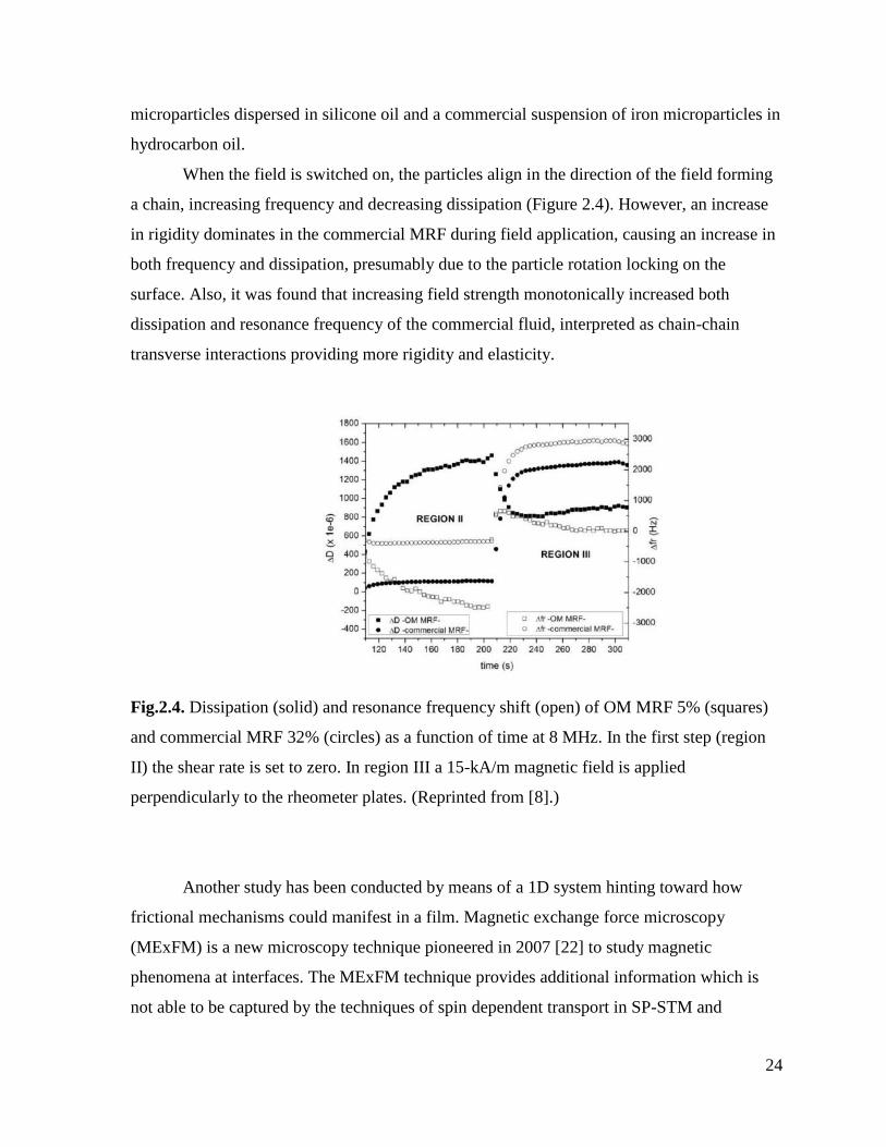
microparticles dispersed in silicone oil and a commercial suspension of iron microparticles in

hydrocarbon oil.

When the field is switched on, the particles align in the direction of the field forming

a chain, increasing frequency and decreasing dissipation (Figure 2.4). However, an increase

in rigidity dominates in the commercial MRF during field application, causing an increase in

both frequency and dissipation, presumably due to the particle rotation locking on the

surface. Also, it was found that increasing field strength monotonically increased both

dissipation and resonance frequency of the commercial fluid, interpreted as chain-chain

transverse interactions providing more rigidity and elasticity.

Fig.2.4. Dissipation (solid) and resonance frequency shift (open) of OM MRF 5% (squares)

and commercial MRF 32% (circles) as a function of time at 8 MHz. In the first step (region

II) the shear rate is set to zero. In region III a 15-kA/m magnetic field is applied

perpendicularly to the rheometer plates. (Reprinted from [8].)

Another study has been conducted by means of a 1D system hinting toward how

frictional mechanisms could manifest in a film. Magnetic exchange force microscopy

(MExFM) is a new microscopy technique pioneered in 2007 [22] to study magnetic

phenomena at interfaces. The MExFM technique provides additional information which is

not able to be captured by the techniques of spin dependent transport in SP-STM and

25

tunneling and magnetic dipole interactions of MFM. In this technique the exchange force

between a magnetized tip and a magnetic unit cell is mapped. This spin structure is able to be

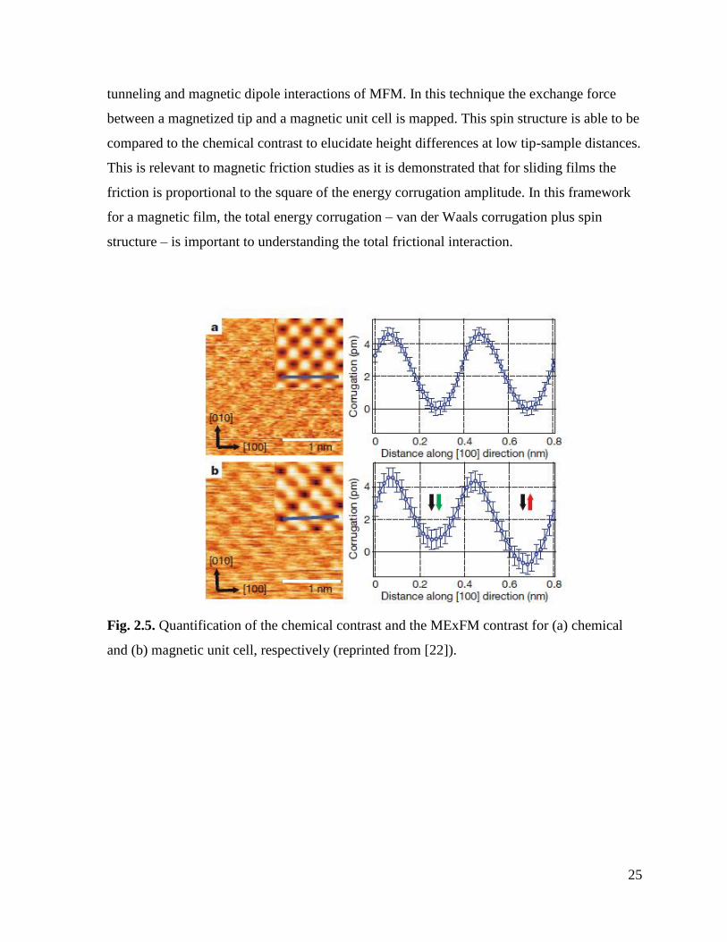
compared to the chemical contrast to elucidate height differences at low tip-sample distances.

This is relevant to magnetic friction studies as it is demonstrated that for sliding films the

friction is proportional to the square of the energy corrugation amplitude. In this framework

for a magnetic film, the total energy corrugation – van der Waals corrugation plus spin

structure – is important to understanding the total frictional interaction.

Fig. 2.5. Quantification of the chemical contrast and the MExFM contrast for (a) chemical

and (b) magnetic unit cell, respectively (reprinted from [22]).

26

2.4. Theoretical and Simulation Studies

Theoretical studies of energy dissipation at a surface are typically molecular

dynamics (MD) or density functional theory (DFT) or analytically solving Landau-Lifshitz-

Gilbert (LLG) equations of motion for a collection of particles each with a moment. Ideally

these situations can be separated into cases in which a tip sliding over substrate, surface-

surface interfactial sliding, and adsorbate film sliding on a surface. For simplicity simulation

studies are categorized here alongside theory.

2.5. Tip-Substrate Sliding

When a cantilever tip approaches a substrate, before physical contact, there has been

observation of anomalously large damping called noncontact friction (NCF) [23]. In recent

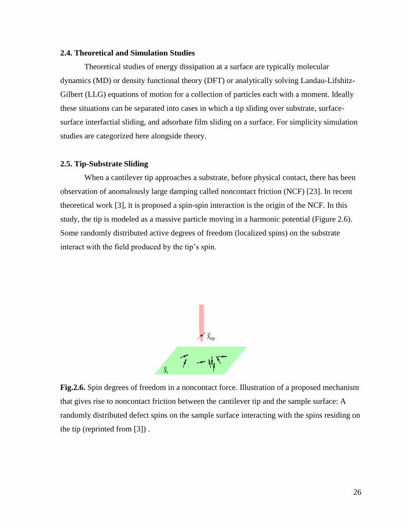
theoretical work [3], it is proposed a spin-spin interaction is the origin of the NCF. In this

study, the tip is modeled as a massive particle moving in a harmonic potential (Figure 2.6).

Some randomly distributed active degrees of freedom (localized spins) on the substrate

interact with the field produced by the tip’s spin.

Fig.2.6. Spin degrees of freedom in a noncontact force. Illustration of a proposed mechanism

that gives rise to noncontact friction between the cantilever tip and the sample surface: A

randomly distributed defect spins on the sample surface interacting with the spins residing on

the tip (reprinted from [3]) .

27

The surface defects have a distribution of relaxation times, resulting in a dissipation

of energy when the tip is moved perpendicular to the substrate. This is a proposed

explanation for the observed distance dependence of the friction coefficient and the induced

spring constant of a cantilever undergoing oscillatory motion. This work provides a means

for experimentalists to gain detailed data on coupling between tip and sample, as well as

surface defect mechanics and magnetic properties of the substrate. Although this work is

important for noncontact friction, it is limited to the case of tip movement in the

perpendicular direction.

There has been recent theory research addressing the situation of the friction of an

MFM tip sliding along a sample laterally [4]. The tip is modeled as a single point dipole and

moves with fixed velocity along the surface composed of a lattice of damped spin precessors.

The precession points relate with their neighbors as well as the tip through magnetic dipole

interactions. The rate of dissipated energy can then be calculated from the total expression

for energy. The system energy is transferred from the tip to the substrate, and then dissipated

by the spin precession.

The velocity dependence of the resultant magnetic friction was predicted to be linear

for small velocities, analogous to macroscopic viscous friction. It was found that this type of

motion can induce spin waves [5], which dissipate energy, which manifests as friction. The

mechanics of the wave front were then explored. A more complex spin dynamics dominates

for increased tip velocities, resulting in a resonance maximum frictional force at ~10^3 m/s.

This work is useful for deeper understanding of the strength of interaction of write head of

magnetic storage or AFM use. It leads the way to experimental studies measuring the effect.

Magnetic dissipation due to spin flip is known to have a temperature dependence,

typically occurring at low temperatures due to the requirement for existing spin order. To

model the substrate, a Heisenberg model is used:

ℋ𝑠𝑢𝑏 = −𝐽 ∑ 𝑺𝑖 ∙ 𝑺𝑖

⟨𝑖,𝑗⟩

− 𝑑𝑧 ∑ 𝑆𝑖,𝑧2

𝑁

𝑖=1

(2.1)

Where J is positive (negative) for ferromagnetic (anti-ferromagnetic) exchange. 𝑑𝑧 is

anisotropy energy constant, which prefers the spins to align in-plane. For ferromagnetic

materials, the dipole-dipole term can be neglected because it is much weaker than the

exchange force. The Heisenberg model is used in a tip scan study on a magnetic monolayer

28

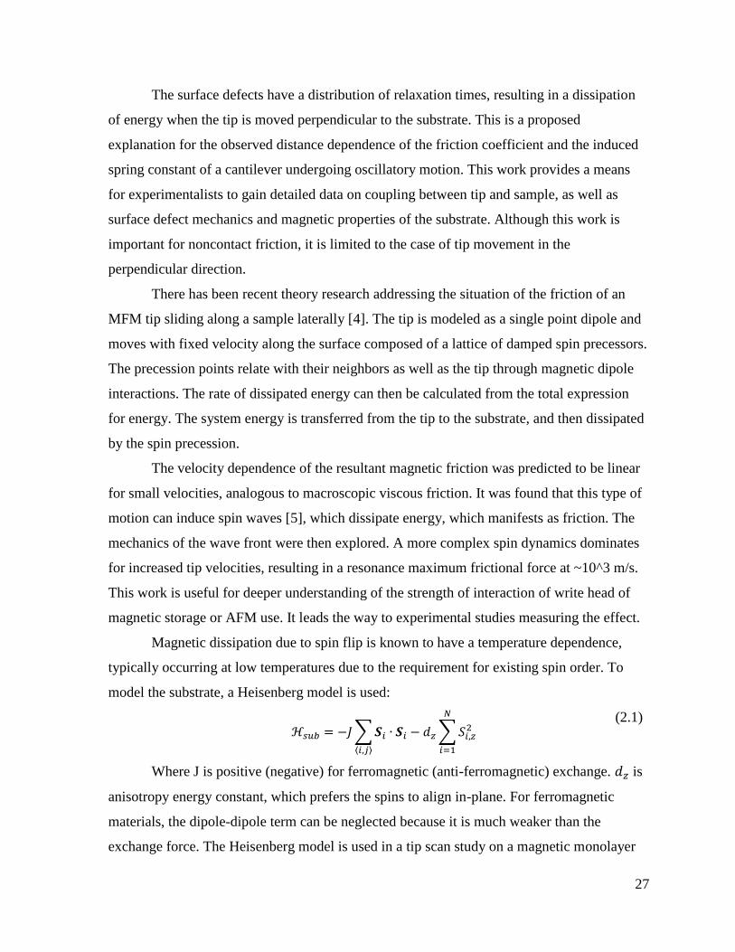
[24] finding the friction to depend linearly on scanning velocity v and LLG damping constant

(Figure 2.7). Increasing temperature beyond kBT = 1.6 J is seen to exponentially decrease

the friction coefficient.

Fig.2.7. Friction coefficients for different α, ωStip and kBT. One can distinguish between a

low-temperature regime where the friction coefficient depends on α but not on ωStip, and a

high-temperature regime, in which it depends on ωStip but not on α (reprinted from [5]).

The explanation for the interdependence of the parameters is thus: At low temperature

near T=0, the undisturbed spin lattice is low in entropy so the damping parameter

dependence of friction dominates. In the high temperature regime beyond kBT ~ 0.7, the

friction results from the tip’s wake of partial order propagated through a disordered system.

Raising the temperature further decreases the radius at which the tip is able to sustain order

whilst sliding along the substrate spin system, and thus decreases friction.

For this analytical study, the tip field is a dipole interaction over a sum of substrate

dipoles and has ‘hard-magnetized’ orientation. As is typical in magnetic dissipation studies,

the LLG equation is used to dynamically describe substrate spins’ damped precession. This

study is unique in that the effect of the temperature bath is modeled as a stochastic term in

the total field equation felt at each site. Taking the Hamiltonian’s partial (total) derivative

with respect to time yields the power pumped between the tip and substrate (total system).

Taking the time average of the explicit power dissipation can yield the magnetic friction

force, as in [25].

29

The dissipation of magnetic vortex states induced in a magnetic substrate by means of

a magnetically polarized tip has been calculated [25]. The substrate is modeled by a grid of

spin moments. The Landau-Lifshitz-Gilbert (LLG) equation is used to describe the dynamics

of the precessing spin moments:

𝜕𝑆𝑖

𝜕𝑡= −

(1 + 2)𝜇𝑠[𝑆𝑖 × ℎ𝑖 + 𝑆𝑖 × (𝑆𝑖 × ℎ𝑖)]

(2.2)

Where 𝑆𝑖 is the substrate spin ith component, t is time, is gyromagnetic ratio, 𝜇𝑠 is

saturation magnetization, damping constant and local field ℎ𝑖. The LLG equation is a

magnetic analogue of a mechanical top axis precessing in a gravity field, and is related to

Larmor precession and is familiar to nuclear magnetic resonance (NMR) and magnetic

resonance imaging (MRI) medical technique. From this, the dissipation can be calculated:

𝑃𝑑𝑖𝑠𝑠 = − ∑ ℎ𝑖

𝑖

∙ 𝜕𝑡𝑆𝑖 (2.3)

And thus the magnetic friction force is taken to be:

𝐹 =

⟨𝑃𝑑𝑖𝑠𝑠⟩

𝑣

(2.4)

Where v is sliding velocity. This is the averaged friction over one atomic interval at steady

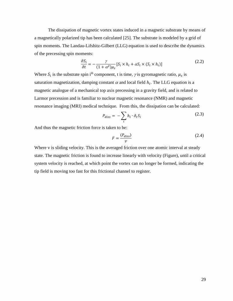
state. The magnetic friction is found to increase linearly with velocity (Figure), until a critical

system velocity is reached, at which point the vortex can no longer be formed, indicating the

tip field is moving too fast for this frictional channel to register.

30

Fig. 2.8. Magnetic friction vs. velocity for systems with a vortex. Above threshold velocities

(depending on α and w), the system makes a transition to a non-vortex state (reprinted from

[25]).

In a related study of tip magnetic dynamics the energy dissipation mechanism has

been identified [6] for magnetic exchange force microscopy (MExFM), in which the tip is

magnetized and magnetic exchange forces with the sample are probed via dissipation in the

resonance of the cantilever at ~160 KHz range. The oscillating magnetic tip induces an

oscillation in the magnetic field which couples to spin moments in the substrate. The

dissipation has been resolved in previously discussed experiments with an Fe tip on NiO

films to be strong for spin moments aligned parallel with the tip moment and negligible for

spin moments aligned anti-parallel [9].

The substrate spin moments are then induced to couple to the phonon bath via the

Caldeira-Leggett framework of quantum dissipation. Quantum mechanics usually deals with

Hamiltonians for which the total energy is conserved, which doesn’t allow for dissipation. To

31

circumvent this issue the Hamiltonian is split into two parts: the quantum system and a bath

of oscillators (phonons), to which energy irreversibly flows. This explanation is consistent

with the results in that dissipation is large (~50meV per cycle), is strong for anti-parallel spin

and negligible for parallel spin (figure), and is relatively independent upon tip oscillation

frequency above the threshold frequency.

Fig. 2.9. Effective potential felt by a tip spin under the effect of the bosonic bath for tip over

spin-up and spin-down configuration. (Reprinted from [6].)

32

2.6 Film-Substrate Sliding

For physisorption of a noble gas on a noble metal substrate a Lennard-Jones potential

describes the interaction of the noble gas atoms with substrate atoms:

𝑉(𝑟) = 4 [(

𝑟)

12

− (

𝑟)

6

] (2.5)

Where r is the inter-atomic distance and and are specific to the two atoms chosen in the

system. When the adsorbed atom slides along the substrate, it experiences a periodic

substrate potential:

𝑉𝑠(𝑥, 𝑧) = ′ [𝑉0(𝑧) + 𝑓𝑉1(𝑧) ∑ cos (𝐺𝑖 ∙ 𝑥)

3

𝑖=1

] (2.6)

Where 𝐺𝑖 are the three reciprocal lattice vectors of the substrate, x is position along sliding

direction, z is distance between adsorbate and first substrate layer, and f is an amplitude-

tuning parameter related the nature of delocalization of the electrons. The larger the ad-atom

and the more itinerant the electrons become, the less f will be. 𝑉0 and 𝑉1 are defined by

Steele [26]. Molecular dynamics algorithms were applied to 40-400 adsorbate atoms on the

surface and coupled to a heat bath, finding a viscous friction law for liquid and

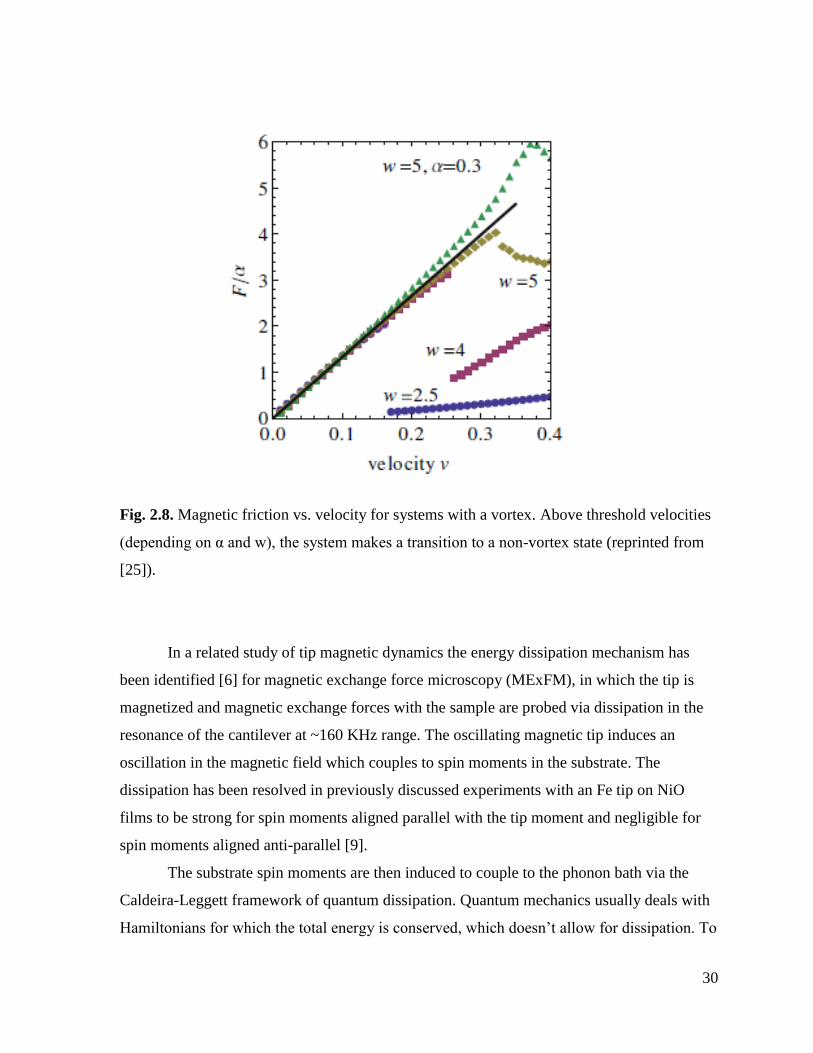
incommensurate solid systems (see figure). The simulation confirms experimental findings

[27] that the slip time of Kr on Au undergoes a transition increasing to a new level as the

coverage increases beyond one monolayer. For a viscous force law, averaging the

corrugation force allows one to calculate:

𝑉𝑠−1 ∝ 𝑓2 (2.7)

Where is slip time. The adsorbate is deformed by the corrugation of the substrate in an

anharmonic fashion, spreading energy into other phonon modes, thus dissipating energy. This

agreement also implies viscous friction laws to be the norm for these physisorption sliding

systems, as has been found experimentally [27].

33

Fig. 2.10. Variation of steady-state velocity v with force per atom F. Results for a

commensurate case at f =0.1 and 0.3 are shown by open and filled squares, respectively.

Results for an incommensurate case that models Kr on Au at kBT/ε = 0.385 and 0.8 are

shown by open and filled circles, respectively. (Reprinted from [2].)

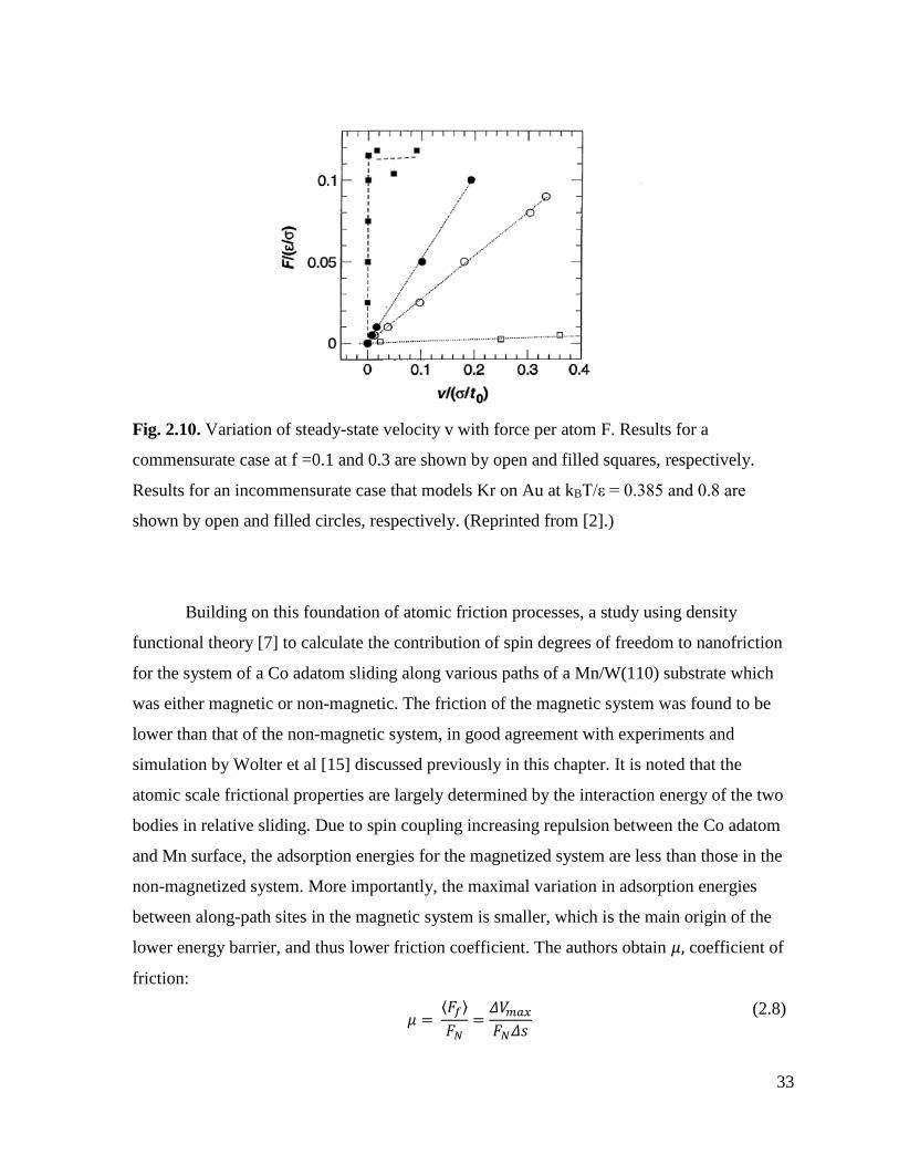
Building on this foundation of atomic friction processes, a study using density

functional theory [7] to calculate the contribution of spin degrees of freedom to nanofriction

for the system of a Co adatom sliding along various paths of a Mn/W(110) substrate which

was either magnetic or non-magnetic. The friction of the magnetic system was found to be

lower than that of the non-magnetic system, in good agreement with experiments and

simulation by Wolter et al [15] discussed previously in this chapter. It is noted that the

atomic scale frictional properties are largely determined by the interaction energy of the two

bodies in relative sliding. Due to spin coupling increasing repulsion between the Co adatom

and Mn surface, the adsorption energies for the magnetized system are less than those in the

non-magnetized system. More importantly, the maximal variation in adsorption energies

between along-path sites in the magnetic system is smaller, which is the main origin of the

lower energy barrier, and thus lower friction coefficient. The authors obtain 𝜇, coefficient of

friction:

𝜇 =

⟨𝐹𝑓⟩

𝐹𝑁=

𝛥𝑉𝑚𝑎𝑥

𝐹𝑁𝛥𝑠

(2.8)

34

where ⟨𝐹𝑓⟩ is averaged friction force, 𝐹𝑁 is applied load, 𝛥𝑉𝑚𝑎𝑥 is potential energy

difference between the maximum and minimum along sliding path under load, and 𝛥𝑠 is

distance along sliding direction. This analysis assumes the total difference in binding energy

to be lost during one cycle, whereas in reality generally only a portion of this energy is

expected to be lost, and therefore over-estimates the sliding friction. However, for

comparison’s sake it is a useful framework for first order calculations of expected sliding

coefficient. It is not clear whether this framework can be used universally, even in systems

which the magnetic ad-atom is non-periodic in structure or is non-uniformly magnetized,

such as in the case of an antiferromagnetic state of oxygen.

Fig. 2.11. Adsorption energies along three sliding paths. Non-spin polarized and spin-

polarized systems are labeled as black and red curves, respectively. The value of energy in

each panel represents the difference of adsorption energies between T and H(B) (reprinted

from [7]).

35

2.7. Planar-Planar Sliding

In a recent theory study, Kadau et al explored the alternate but experimentally

accessible geometry in which the magnetic friction occurs between two planar surfaces

sliding on each other [28]. In this study, only nonmetallic ferromagnetic materials were

modeled. Phononic and electronic dissipation mechanisms were not accounted for (to

highlight magnetic effects) but included in a heat bath. A 2D square lattice of sites carrying

spins was simulated in Monte Carlo. The opposing lattices interacted with each other and the

heat bath. Energy was pumped into the system by sliding one lattice over the other at 10^-2

m/s. Beyond a plane size of 20 lattice constants, the magnetic friction force is found to be

proportional to the length of the cell along the direction of motion, as one might expect.

This shows that the energy pumped into the spin degrees of freedom gets transferred

to the heat bath before driving nonlocal sites. The dependence of the dissipation rate upon

velocity is found to be linear, but tails off at higher velocities at different rates for different

dynamics models. A slice of finite thickness was considered also in the place of a 2D plane.

For this situation, it was concluded that magnetic friction would not be too weak to be

observable, in comparison to ordinary solid friction. This setup would be consistent with a

QCM experiment in which two or more thin films of magnetic material were adsorbed one

on top the other and set sliding against each other.

36

2.8. Molecular Oxgyen Adsorption in 2D

To explore the question of magnetic dissipation mechanisms in 2D systems, we look

at oxygen films on various substrates. Oxygen’s unique molecular magnetism provides a

useful environment for the question to be answered. It exhibits a rich phase diagram in 2D

and bulk, due in part to the interactions of the molecular spin moments. In the following

pages we present studies of oxygen phase structure on various substrates. In these studies, the

substrates were held stationary, and so frictional dissipation occurring at equilibrium cannot

be accounted for – diffusion is however observed in some of the original studies.

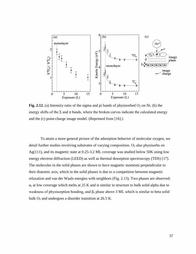
The first of these studied the substrate of a bare Ni(111) in the presence of oxygen

molecules, wherein the oxygen dissociates and chemisorbs onto nickel, forming a p(2x2)

overlayer of NiO. Aoki et al [16] using metastable atom electron microscopy provide details

as to the electronic states of physisorbed O2 atop this oxide layer at 20K and 293K. Their

spectra indicate that a monolayer of physisorbed O2 at 20K lie down on the chemisorbed O2

with axes parallel, and with increasing coverage the axis tilts gradually upwards, as is seen

for O2 on graphite situation. This study was conducted for stationary substrate, and provides

a framework for oxygen’s behavior at low temperature in static equilibrium. The question

that seeks to be answered is that of dissipation channels across the interface when the Ni and

O2 film are sliding with respect to one another.

37

Fig. 2.12. (a) Intensity ratio of the sigma and pi bands of physisorbed O2 on Ni. (b) the

energy shifts of the Σ and π bands, where the broken curves indicate the calculated energy

and the (c) point-charge image model. (Reprinted from [16].)

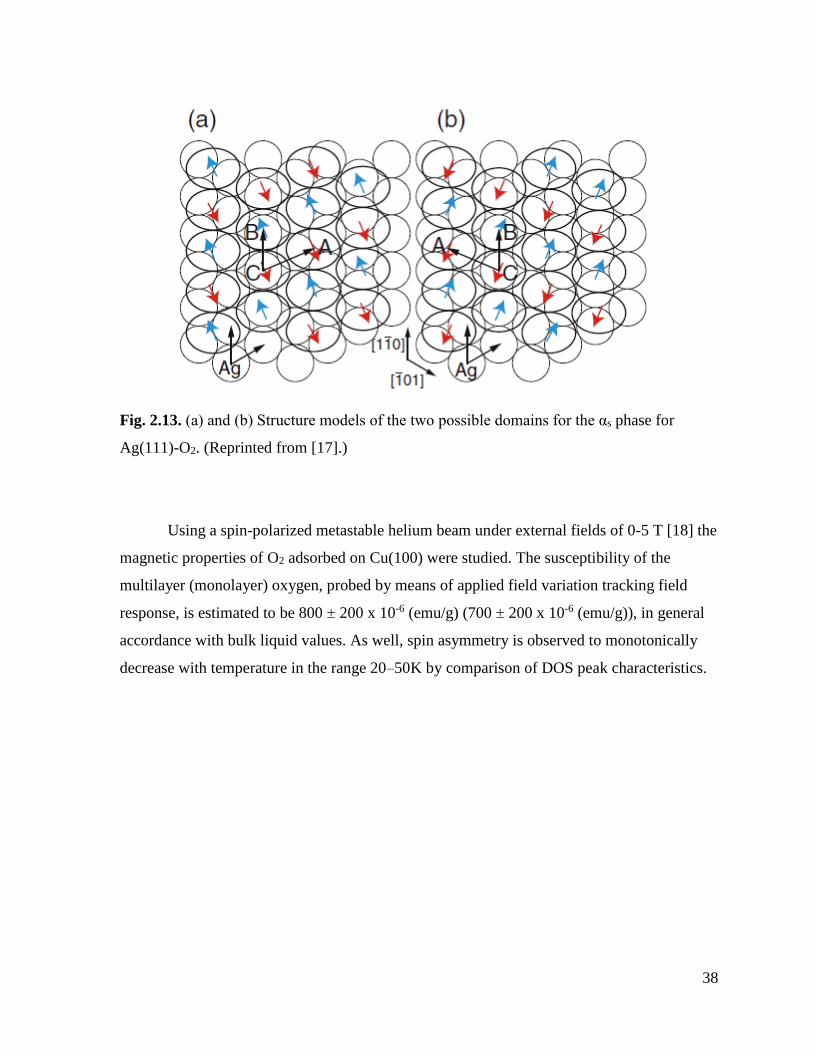
To attain a more general picture of the adsorption behavior of molecular oxygen, we

detail further studies involving substrates of varying composition. O2 also physisorbs on

Ag(111), and its magnetic state at 0.25-3.2 ML coverage was studied below 50K using low

energy electron diffraction (LEED) as well as thermal desorption spectroscopy (TDS) [17].

The molecules in the solid phases are shown to have magnetic moments perpendicular to

their diatomic axis, which in the solid phases is due to a competition between magnetic

relaxation and van der Waals energies with neighbors (Fig. 2.13). Two phases are observed:

αs at low coverage which melts at 25 K and is similar in structure to bulk solid alpha due to

weakness of physisorption bonding, and βs phase above 3 ML which is similar to beta solid

bulk O2 and undergoes a disorder transition at 26.5 K.

38

Fig. 2.13. (a) and (b) Structure models of the two possible domains for the αs phase for

Ag(111)-O2. (Reprinted from [17].)

Using a spin-polarized metastable helium beam under external fields of 0-5 T [18] the

magnetic properties of O2 adsorbed on Cu(100) were studied. The susceptibility of the

multilayer (monolayer) oxygen, probed by means of applied field variation tracking field

response, is estimated to be 800 ± 200 x 10-6 (emu/g) (700 ± 200 x 10-6 (emu/g)), in general

accordance with bulk liquid values. As well, spin asymmetry is observed to monotonically

decrease with temperature in the range 20–50K by comparison of DOS peak characteristics.

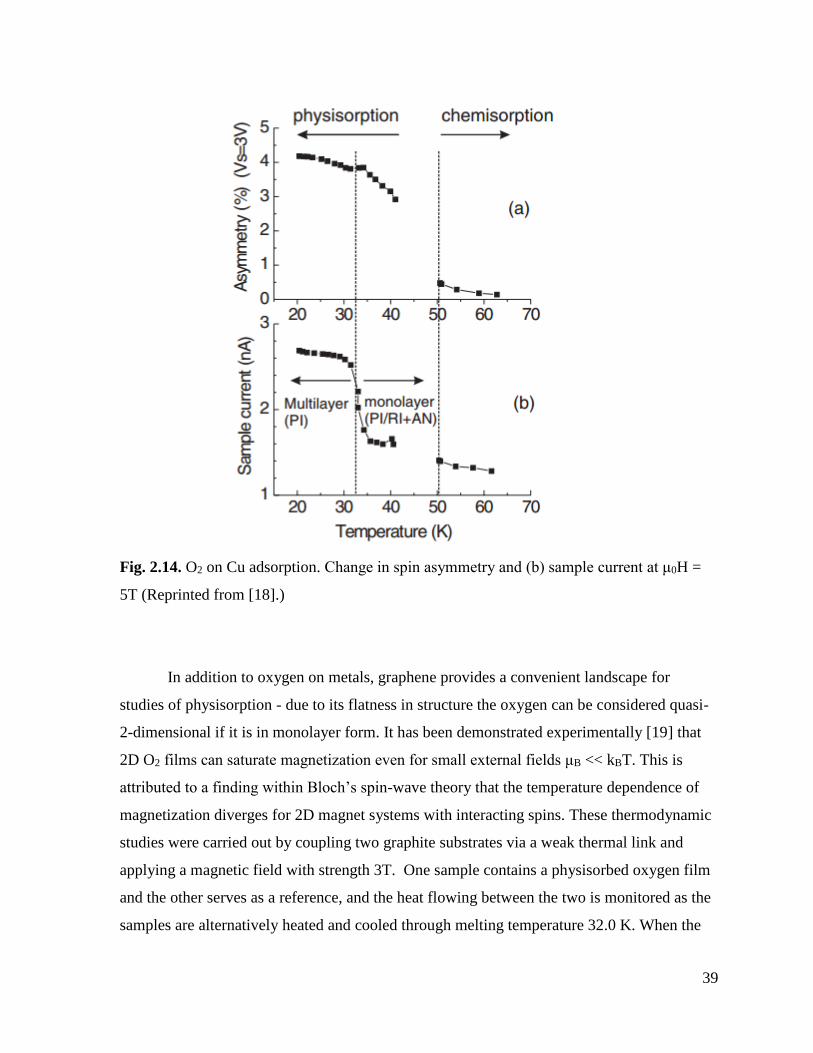
39

Fig. 2.14. O2 on Cu adsorption. Change in spin asymmetry and (b) sample current at μ0H =

5T (Reprinted from [18].)

In addition to oxygen on metals, graphene provides a convenient landscape for

studies of physisorption - due to its flatness in structure the oxygen can be considered quasi-

2-dimensional if it is in monolayer form. It has been demonstrated experimentally [19] that

2D O2 films can saturate magnetization even for small external fields μB << kBT. This is

attributed to a finding within Bloch’s spin-wave theory that the temperature dependence of

magnetization diverges for 2D magnet systems with interacting spins. These thermodynamic

studies were carried out by coupling two graphite substrates via a weak thermal link and

applying a magnetic field with strength 3T. One sample contains a physisorbed oxygen film

and the other serves as a reference, and the heat flowing between the two is monitored as the

samples are alternatively heated and cooled through melting temperature 32.0 K. When the

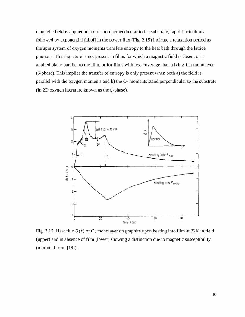
40

magnetic field is applied in a direction perpendicular to the substrate, rapid fluctuations

followed by exponential falloff in the power flux (Fig. 2.15) indicate a relaxation period as

the spin system of oxygen moments transfers entropy to the heat bath through the lattice

phonons. This signature is not present in films for which a magnetic field is absent or is

applied plane-parallel to the film, or for films with less coverage than a lying-flat monolayer

(δ-phase). This implies the transfer of entropy is only present when both a) the field is

parallel with the oxygen moments and b) the O2 moments stand perpendicular to the substrate

(in 2D oxygen literature known as the -phase).

Fig. 2.15. Heat flux 𝑄(𝑡)̇ of O2 monolayer on graphite upon heating into film at 32K in field

(upper) and in absence of film (lower) showing a distinction due to magnetic susceptibility

(reprinted from [19]).

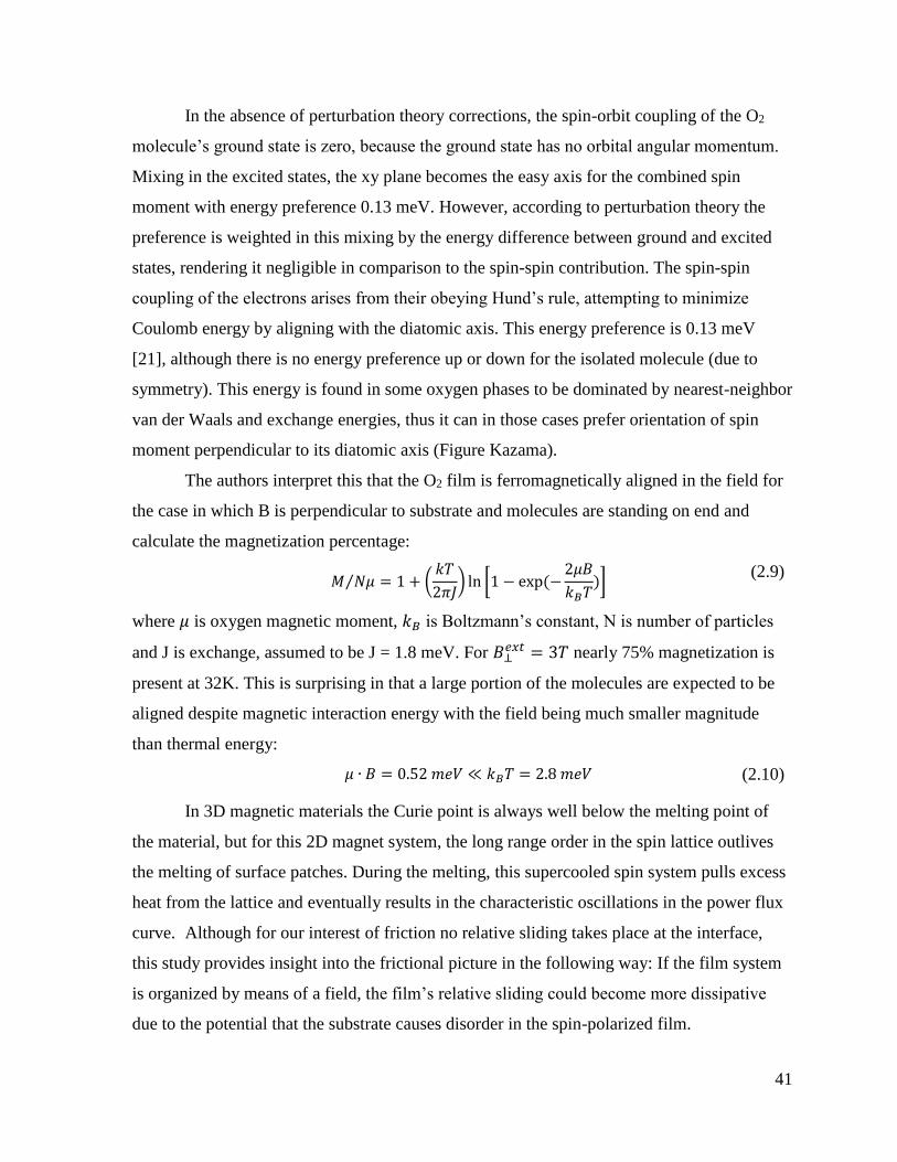
41

In the absence of perturbation theory corrections, the spin-orbit coupling of the O2

molecule’s ground state is zero, because the ground state has no orbital angular momentum.

Mixing in the excited states, the xy plane becomes the easy axis for the combined spin

moment with energy preference 0.13 meV. However, according to perturbation theory the

preference is weighted in this mixing by the energy difference between ground and excited

states, rendering it negligible in comparison to the spin-spin contribution. The spin-spin

coupling of the electrons arises from their obeying Hund’s rule, attempting to minimize

Coulomb energy by aligning with the diatomic axis. This energy preference is 0.13 meV

[21], although there is no energy preference up or down for the isolated molecule (due to

symmetry). This energy is found in some oxygen phases to be dominated by nearest-neighbor

van der Waals and exchange energies, thus it can in those cases prefer orientation of spin

moment perpendicular to its diatomic axis (Figure Kazama).

The authors interpret this that the O2 film is ferromagnetically aligned in the field for

the case in which B is perpendicular to substrate and molecules are standing on end and

calculate the magnetization percentage:

𝑀 𝑁𝜇⁄ = 1 + (

𝑘𝑇

2𝜋𝐽) ln [1 − exp (−

2𝜇𝐵

𝑘𝐵𝑇)]

(2.9)

where 𝜇 is oxygen magnetic moment, 𝑘𝐵 is Boltzmann’s constant, N is number of particles

and J is exchange, assumed to be J = 1.8 meV. For 𝐵⊥𝑒𝑥𝑡 = 3𝑇 nearly 75% magnetization is

present at 32K. This is surprising in that a large portion of the molecules are expected to be

aligned despite magnetic interaction energy with the field being much smaller magnitude

than thermal energy:

𝜇 ∙ 𝐵 = 0.52 𝑚𝑒𝑉 ≪ 𝑘𝐵𝑇 = 2.8 𝑚𝑒𝑉 (2.10)

In 3D magnetic materials the Curie point is always well below the melting point of

the material, but for this 2D magnet system, the long range order in the spin lattice outlives

the melting of surface patches. During the melting, this supercooled spin system pulls excess

heat from the lattice and eventually results in the characteristic oscillations in the power flux

curve. Although for our interest of friction no relative sliding takes place at the interface,

this study provides insight into the frictional picture in the following way: If the film system

is organized by means of a field, the film’s relative sliding could become more dissipative

due to the potential that the substrate causes disorder in the spin-polarized film.

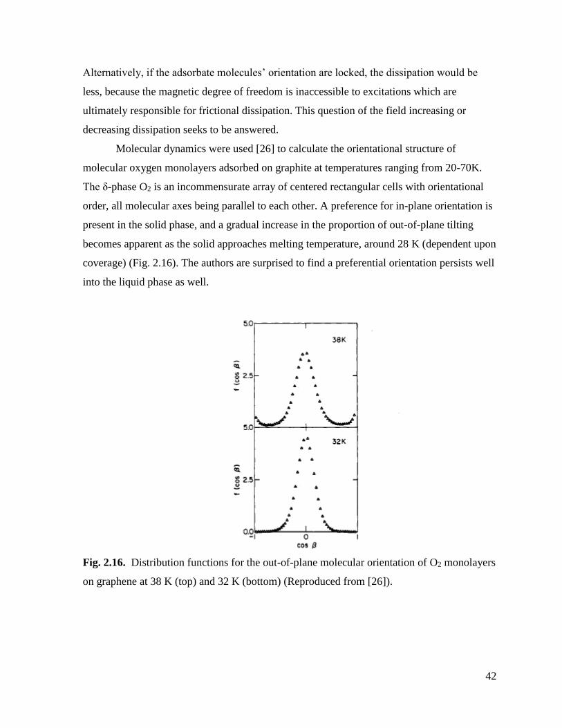
42

Alternatively, if the adsorbate molecules’ orientation are locked, the dissipation would be

less, because the magnetic degree of freedom is inaccessible to excitations which are

ultimately responsible for frictional dissipation. This question of the field increasing or

decreasing dissipation seeks to be answered.

Molecular dynamics were used [26] to calculate the orientational structure of

molecular oxygen monolayers adsorbed on graphite at temperatures ranging from 20-70K.

The δ-phase O2 is an incommensurate array of centered rectangular cells with orientational

order, all molecular axes being parallel to each other. A preference for in-plane orientation is

present in the solid phase, and a gradual increase in the proportion of out-of-plane tilting

becomes apparent as the solid approaches melting temperature, around 28 K (dependent upon

coverage) (Fig. 2.16). The authors are surprised to find a preferential orientation persists well

into the liquid phase as well.

Fig. 2.16. Distribution functions for the out-of-plane molecular orientation of O2 monolayers

on graphene at 38 K (top) and 32 K (bottom) (Reproduced from [26]).

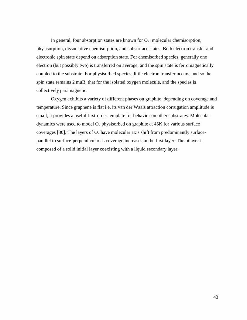
43

In general, four absorption states are known for O2: molecular chemisorption,

physisorption, dissociative chemisorption, and subsurface states. Both electron transfer and

electronic spin state depend on adsorption state. For chemisorbed species, generally one

electron (but possibly two) is transferred on average, and the spin state is ferromagnetically

coupled to the substrate. For physisorbed species, little electron transfer occurs, and so the

spin state remains 2 muB, that for the isolated oxygen molecule, and the species is

collectively paramagnetic.

Oxygen exhibits a variety of different phases on graphite, depending on coverage and

temperature. Since graphene is flat i.e. its van der Waals attraction corrugation amplitude is

small, it provides a useful first-order template for behavior on other substrates. Molecular

dynamics were used to model O2 physisorbed on graphite at 45K for various surface

coverages [30]. The layers of O2 have molecular axis shift from predominantly surface-

parallel to surface-perpendicular as coverage increases in the first layer. The bilayer is

composed of a solid initial layer coexisting with a liquid secondary layer.

44

Fig. 2.17. Projections in the plane of simulations of O2 films on graphite for various surface

coverages. (Reprinted from [30]).

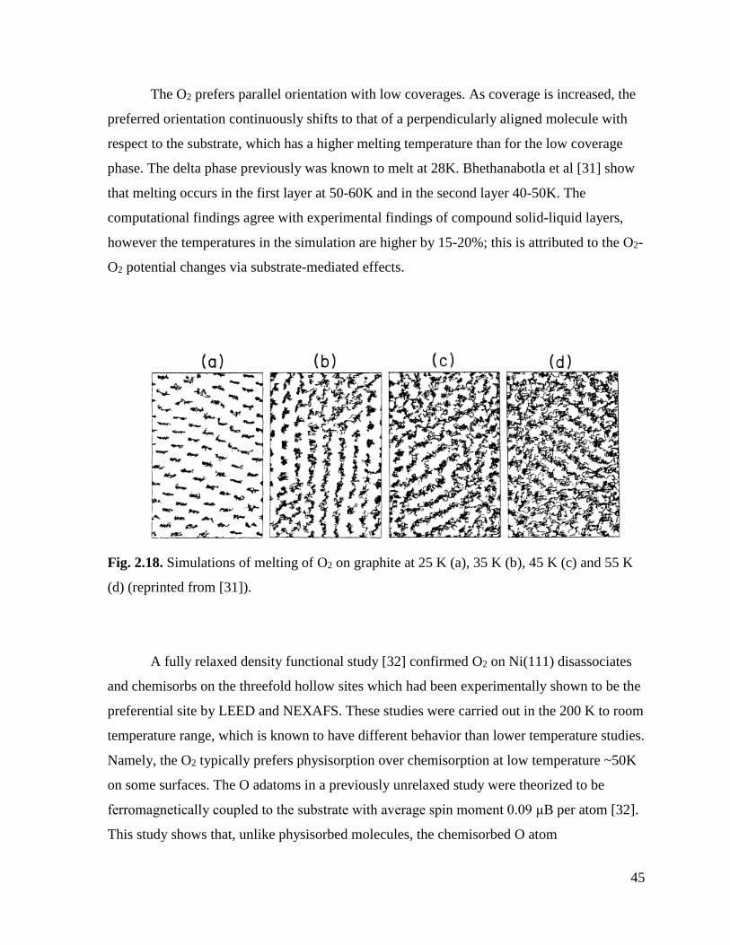
45

The O2 prefers parallel orientation with low coverages. As coverage is increased, the

preferred orientation continuously shifts to that of a perpendicularly aligned molecule with

respect to the substrate, which has a higher melting temperature than for the low coverage

phase. The delta phase previously was known to melt at 28K. Bhethanabotla et al [31] show

that melting occurs in the first layer at 50-60K and in the second layer 40-50K. The

computational findings agree with experimental findings of compound solid-liquid layers,

however the temperatures in the simulation are higher by 15-20%; this is attributed to the O2-

O2 potential changes via substrate-mediated effects.

Fig. 2.18. Simulations of melting of O2 on graphite at 25 K (a), 35 K (b), 45 K (c) and 55 K

(d) (reprinted from [31]).

A fully relaxed density functional study [32] confirmed O2 on Ni(111) disassociates

and chemisorbs on the threefold hollow sites which had been experimentally shown to be the

preferential site by LEED and NEXAFS. These studies were carried out in the 200 K to room

temperature range, which is known to have different behavior than lower temperature studies.

Namely, the O2 typically prefers physisorption over chemisorption at low temperature ~50K

on some surfaces. The O adatoms in a previously unrelaxed study were theorized to be

ferromagnetically coupled to the substrate with average spin moment 0.09 μB per atom [32].

This study shows that, unlike physisorbed molecules, the chemisorbed O atom

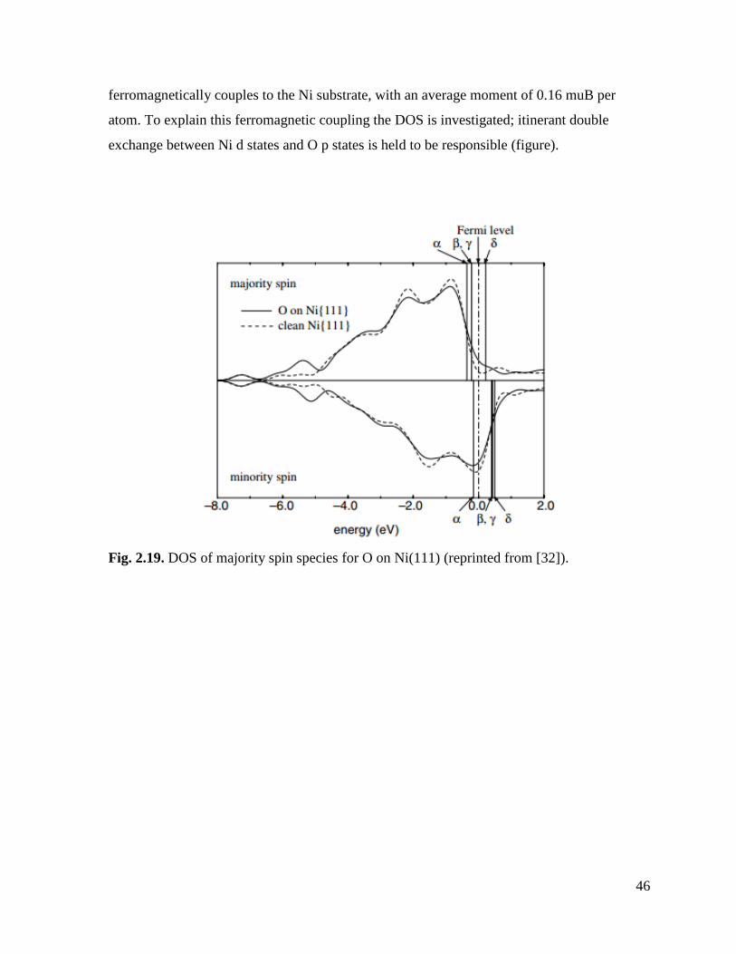
46

ferromagnetically couples to the Ni substrate, with an average moment of 0.16 muB per

atom. To explain this ferromagnetic coupling the DOS is investigated; itinerant double

exchange between Ni d states and O p states is held to be responsible (figure).

Fig. 2.19. DOS of majority spin species for O on Ni(111) (reprinted from [32]).

47

2.9. Towards answering these open questions

This chapter has laid out some of the recent forays discovering the ways in which magnetism

and frictional dissipation are intertwined. However, several questions remain, the most

prominent of which are:

A. The Altfeder [10] and Highland [12] studies, as well as the Mistura [13,14] studies

showed that a magnetic field could alter the superconductivity state then alter friction

indirectly. Is a similar behavior present in systems whose magnetic state behavior is

altered directly?

B. The Mistura studies required a thermal annealing to record friction measurements at

cryogenic temperatures. Is this required in general?

C. In the Wiesendanger [9,22] studies, a new microscopy technique was invented that

relies on magnetic dissipation of a tip in contact with a magnetic substrate - no

experiment has determined whether this dissipation carries over into two dimensions.

D. The Johannesmann [8] experiment observed magnetorheological fluid’s dissipation

being altered by a field. How can this be understood in a frictional framework?

E. MExFM [22] have shown spin contrast superimposed on vdW lattice. In the

framework of Cieplak [2], does this affect the friction of a film’s sliding in a way that

is observable?

F. The Kadau study [28] predicted that the magnetic damping would be observable in

2D systems but this has yet to be shown experimentally.

G. Cai [7] conducted simulations of a magnetic monolayer on a magnetic substrate find a

decreased total friction, due to the spin friction. This behavior has yet to be

experimentally observed, especially to find whether the behavior changes in the case

the adsorbate magnetism is not rigidly locked (as in the Wiesendanger tip studies).

H. The studies on oxygen adsorption on graphene [19,29-33] and metals [16-19] point to

the ability to alter the molecular orientation. Could this control extend to the friction

levels?

Some of the previously discussed studies have provided insight into oxygen-film

adsorption, which serves as a convenient model system for magnetic sliding friction

experiments. In the following chapter, I detail an experimental apparatus capable of

48

measuring the friction between adsorbate films and their substrates set into relative sliding in

an effort to answer some of the questions toward which this previous literature has hinted.

Adsorbate-substrate systems I study are O2 on Ni, O2 on Au, N2 on Au, and O2 on Fe-

Bipy/Au. Parameters which are accessible to control are applied field strength; film

thickness, composition, phase, and magnetic state; temperature; and substrate composition

and magnetic state. The aim is to make comparisons on the variations introduced by

changing these parameters and thus elucidate the nature of magnetic frictional behavior in a

nanoscale film-substrate system.

In the process of this experimentation, I have answered questions A, B, C, D, E, F, G

and most prominently H.

49

REFERENCES CHAPTER 2

[1] Krim, J. (1991). Sliding friction measurements of molecularly thin films. Journal of

Vacuum Science & Technology A: Vacuum, Surfaces, and Films, 9(1991), 2566.

http://doi.org/10.1116/1.577274

[2] Cieplak, M., Smith, E. D., & Robbins, M. (1994). Molecular Origins of Friction : The

Force on Adsorbed Layers, 265(5176), 1209–1212.

[3] She, J. H., & Balatsky, A. V. (2012). Noncontact friction and relaxational dynamics of

surface defects. Physical Review Letters, 108(March), 1–5.

http://doi.org/10.1103/PhysRevLett.108.136101

[4] Fusco, C., Wolf, D., & Nowak, U. (2008). Magnetic friction of a nanometer-sized tip

scanning a magnetic surface: Dynamics of a classical spin system with direct exchange and

dipolar interactions between the spins. Physical Review B, 77, 174426.

http://doi.org/10.1103/PhysRevB.77.174426

[5] Magiera, M. P., Brendel, L., Wolf, D. E., & Nowak, U. (2011). Spin waves cause non-

linear friction. Europhysics Letters, 95, 17010. http://doi.org/10.1209/0295-5075/95/17010

[6] Pellegrini, F., Santoro, G. E., & Tosatti, E. (2010). Atomic spin-sensitive dissipation on

magnetic surfaces. Physical Review Letters, 105(October), 1–4.

http://doi.org/10.1103/PhysRevLett.105.146103

[7] Cai, X., Wang, J., Li, J., Sun, Q., & Jia, Y. (2016). Spin friction between Co monolayer

and Mn/W(110) surface: Ab Initio investigations. Tribology International, 95, 419–425.

http://doi.org/10.1016/j.triboint.2015.11.037

[8] Rodriguez-López, J., Castro, P., de Vicente, J., Johannsmann, D., Elvira, L., Morillas, J.,

& Montero de Espinosa, F. (2015). Colloidal Stability and Magnetic Field-Induced Ordering

of Magnetorheological Fluids Studied with a Quartz Crystal Microbalance. Sensors, 15,

30443–30456. http://doi.org/10.3390/s151229808

50

[9] Wolter, B., Yoshida, Y., Kubetzka, A., Hla, S. W., Von Bergmann, K., & Wiesendanger,

R. (2012). Spin friction observed on the atomic scale. Physical Review Letters,

109(SEPTEMBER), 1–5. http://doi.org/10.1103/PhysRevLett.109.116102

[10] Highland, M., & Krim, J. (2006). Superconductivity Dependent Friction of Water,

Nitrogen, and Superheated He Films Adsorbed on Pb(111). Physical Review Letters,

96(June), 226107. http://doi.org/10.1103/PhysRevLett.96.226107

[11] Bruch, L. (2000). Ohmic damping of center-of-mass oscillations of a molecular

monolayer. Physical Review B, 61(23), 16201–16206.

http://doi.org/10.1103/PhysRevB.61.16201

[12] Altfeder, I., & Krim, J. (2012). Temperature dependence of nanoscale friction for Fe on

YBCO. Journal of Applied Physics, 111, 094916. http://doi.org/10.1063/1.4717983

[13] Bruschi, L., Pierno, M., Fois, G., Ancilotto, F., Mistura, G., Boragno, C., … Valbusa, U.

(2010). Friction reduction of Ne monolayers on preplated metal surfaces. Physical Review B

- Condensed Matter and Materials Physics, 81, 1–5.

http://doi.org/10.1103/PhysRevB.81.115419

[14] Bruschi, L., Fois, G., Pontarollo, a., Mistura, G., Torre, B., Buatier De Mongeot, F., …

Valbusa, U. (2006). Structural depinning of Ne monolayers on Pb at T<6.5K. Physical

Review Letters, 96(June), 2–5. http://doi.org/10.1103/PhysRevLett.96.216101

[15] Ouazi, S., Kubetzka, A., von Bergmann, K., & Wiesendanger, R. (2014). Enhanced

Atomic-Scale Spin Contrast due to Spin Friction. Physical Review Letters, 112, 076102.

[16] Aoki, M., Taoka, H., Kamada, T., & Masuda, S. (2001). Local electronic states of

oxygen on Ni(111) surface studied by metastable atom electron spectroscopy. Journal of

Electron Spectroscopy and Related Phenomena, 114-116 (2001) 507-512.

[17] Kazama, Y., Matsumoto, M., Sugimoto, T., Okano, T., & Fukutani, K. (2011). Low-

temperature surface phase and phase transition of physisorbed oxygen on the Ag(111)

surface. Physical Review B - Condensed Matter and Materials Physics, 84(April), 4–6.

http://doi.org/10.1103/PhysRevB.84.064128

51

[18] Kurahashi, M., Sun, X., & Yamauchi, Y. (2012). Magnetic properties of O2 adsorbed on

Cu(100): A spin-polarized metastable He beam study. Physical Review B - Condensed

Matter and Materials Physics, 86, 1–2. http://doi.org/10.1103/PhysRevB.86.245421

[19] Marx, R., & Christoffer, B. (1985). Magnetocaloric effects of 2D adsorbed O2. Journal

of Physics C: Solid State Physics, 18, 2849–2858. http://doi.org/10.1088/0022-

3719/18/14/016

[21] Herzberg, G. (1939). Molecular Spectra and Molecular Structure I. Diatomic

Molecules. New York: Prentice Hall, Inc.

[22] Kaiser, U., Schwarz, a., & Wiesendanger, R. (2007). Magnetic exchange force

microscopy with atomic resolution. Nature, 446(March), 522–525.

http://doi.org/10.1038/nature05617

[23] Stipe, B. C., Mamin, H. J., Stowe, T. D., Kenny, T. W., & Rugar, D. (2001). Noncontact

Friction and Force Fluctuations between Closely Spaced Bodies. Physical Review Letters, 87,

096801. http://doi.org/10.1103/PhysRevLett.87.096801

[24] Magiera, M. P., Wolf, D. E., Brendel, L., & Nowak, U. (2009). Magnetic Friction and

the Role of Temperature. IEEE Trans. Magn., 45(10), 3938–3941.

http://doi.org/10.1109/TMAG.2009.2023623

[25] Magiera, M. P. (2013). Energy dissipation of moved magnetic vortices. EPL

(Europhysics Letters), 103, 57004. http://doi.org/10.1209/0295-5075/103/57004

[26] Bhethanabotla, V. R., & Steele, W. a. (1987). Molecular dynamics simulations of

oxygen monolayers on graphite. Langmuir, 3, 581–587. http://doi.org/10.1021/la00076a025

[27] Krim, J., Solina, D. H., & Chiarello, R. (1991). Nanotribology of a Kr monolayer: A

quartz-crystal microbalance study of atomic-scale friction. Physical Review Letters.

http://doi.org/10.1103/PhysRevLett.66.181

52

[28] Kadau, D., Hucht, A., & Wolf, D. E. (2008). Magnetic friction in Ising spin systems.

Physical Review Letters, 101(September), 1–4.

http://doi.org/10.1103/PhysRevLett.101.137205

[30] Bhethanabotla, V.R., & Steele, W. (1987). Simulations of O2 adsorbed on graphite at

45K: the monolayer to bilayer transition. Can. J. Chem. 66, 866.

[31] Bhethanabotla, V.R., & Steele, W. (1990). Computer-simulation study of melting in

dense oxygen layers on graphite. Physical Review B. 41-13.

[32] Yamagishi, S., Jenkins, S. J., & King, D. a. (2003). First principles studies of

chemisorbed O on Ni{1 1 1}. Surface Science, 543(April), 12–18.

http://doi.org/10.1016/j.susc.2003.08.002

53

CHAPTER 3: EXPERIMENTAL SETUP

This chapter describes my quartz crystal microbalance samples, how a QCM

measures friction, and the UHV cryogenic gas dosage apparatus which I built to acquire data,

as well as details about sample preparation. All data taken in this dissertation have been on

the QCMs described here.

3.1. Quartz crystal microbalance – a general description

The quartz crystal microbalance (QCM) was historically used as a timing device and

later as a mass uptake probe, and in 1988 the possibility of its use as a nanofrictional probe

was first demonstrated by Krim and Widom [1]. QCMs are used today in a wide array of

research areas including but not limited to thin film growth; polymer films; liquid

environments; gas adsorbates; UHV vacuum conditions; nanoparticle lubricants; as

immunosensors of proteins, antibodies, bacteria and viruses; SAMS film formation; and

DNA biosensors [2]. Our QCM samples are AT-cut with resonance frequency 8.01 MHz and

overtone polished by Laptech Precision Inc [3]. The disk is 200 μm in thickness and 0.375”

in diameter.

The Curie brothers were the first to discover the piezoelectric effect in quartz.

Piezoelectricity is defined as a material’s induced voltage response to applied stress, and vice

versa. In this way a piezoelectric material’s strain vector and voltage are coupled into a

response tensor. Quartz crystals are composed of one silicon atom and two oxygen atoms in

their basic structure. The formula SiO2 is shared with sand and glass and is the second most

abundant molecule on the earth. The ways in which the superstructure is organized

determines which substance emerges macroscopically. In glass the molecular structure is

amorphous, having no preferred direction or repeated structure as it branches outward.

-Quartz has trigonal crystal structure, meaning there is one threefold axis of

rotation. This axis is labeled the Z axis. Two unit vectors of the base cell are of the same

length, the remaining is of a stretched length in comparison. All three angles of the base

structure are 90o. Above 573 C temperature threshold, alpha quartz transforms into beta

quartz, gaining hexagonal symmetry and losing its piezoelectric property in the process,

which cannot be fully regained after cooling. -Quartz for oscillator purposes is sliced along

54

a direction with respect to different axes for different purposes: X-cut, Y-cut, AT-cut, and

BT-cut being several options. X-cut provides a parallel response of applied strain vector and

field lines, thus oscillations occur in breathing mode. Y-cut provides a strong temperature

dependence upon frequency. The AT-cut slice direction is 35 degrees and 15 minutes from

the Z axis such that it contains the X axis. AT-cut is typically used for QCMs because of its

shear wave response and flat frequency dependence on temperature in the vicinity of room

temperature.

3.2. Mass uptake with QCM technique

The unloaded QCM is effectively treated as a damped, driven simple harmonic

oscillator wherein the damping occurs in internal friction, driving is done by the Pierce

circuitry voltage modulation, and the oscillatory motion occurs due to piezoelectric coupling

of strain and applied voltage. In 1959 Sauerbrey treated mass adsorption on a QCM face as

an incremental increase in the thickness of the disk [4]. Due to the piezoelectric response, an

applied voltage couples to a strain field in the crystal. Applying a voltage at the surface

electrode of a QCM causes a sound wave to begin to propagate through the crystal. The

acoustic shear wave propagates from one electrode to the opposite electrode through the

quartz crystal bulk at constant velocity:

𝑐𝑞 = λ𝑓0 (3.1)

Where 𝑐𝑞 is the speed of a transverse sound wave in quartz, λ is its wavelength and 𝑓0 is its

frequency. Here we deal with modes of excitation in which a half wavelength fits into the

width of the crystal:

𝑡𝑞 =

1

2λ

(3.2)

where 𝑡𝑞 is the thickness of the quartz crystal. When a film is grown on the surface of an

electrode, the thickness of the oscillator is increased, which increases the wavelength, and

thus the frequency shifts:

𝑐𝑞 = λ′𝑓′ (3.3)

where λ′ is the shifted wavelength and 𝑓′ is the shifted frequency. The final oscillator

thickness 𝑡′ can be expressed as the sum of the thickness of the quartz plate 𝑡𝑞 and 𝑡𝑓 the film

thickness:

55

𝑡′ = 𝑡𝑞 + 𝑡𝑓 . (3.4)

The film’s mass density can be written:

ρ𝑓 =

1

𝐴

𝑚𝑓

𝑡𝑓

(3.5)

Where 𝑚𝑓 is mass of the film and 𝐴 is film area. Using equations (1) and (2) we can re-

express 𝑓0 as:

𝑓0 =𝑐𝑞

2𝑡𝑞 . (3.6)

Holding 𝑐𝑞constant, we can take the derivative of resonant frequency with respect to

thickness change:

𝑑𝑓0

𝑑𝑡𝑞=

−𝑐𝑞

2𝑡𝑞2 .

(3.7)

Dividing equation (7) by equation (6) we have:

𝑑𝑓0

𝑓0=

−𝑑𝑡𝑞

𝑡𝑞 .

(3.8)

We can also use equation (5) to re-express in terms of film mass:

𝑚𝑓 = ρ𝑓𝐴𝑡𝑓 (3.9)

or, taking a derivative:

𝑑𝑚𝑓

ρ𝑓𝐴= 𝑑𝑡𝑓 .

(3.10)

Sauerbrey’s treatment was to consider this infinitesimal change in film thickness 𝑑𝑡𝑓 as a

change in quartz oscillator thickness 𝑑𝑡𝑞 [4]. Plugging this into equation (8) gives us:

𝑑𝑓0

𝑓0=

−𝑑𝑚𝑓

ρ𝑓𝐴𝑡𝑞 .

(3.11)

Under small mass loading 𝑑𝑚𝑓 ≪ 𝑚𝑞 , this implies:

Δf =

−Δ𝑚𝑓

𝐴

𝑓02

ρ𝑓𝑣𝑞 .

(3.12)

Which is the Sauerbrey equation used very commonly by nanotribologists [5,6] for one-sided

film growth (vq = cq). For our situation of two-sided film growth, the equation becomes:

ρ2 = −2.221 ∗ 105 ∗

Δf

𝑓02

(3.13)

56

With ρ2 the coverage of the film in g/cm2. By measuring the frequency shifts we can then

detect the level of mass uptake of thin films on the surface electrode of a QCM - this is the

microbalance aspect of the QCM.

57

3.3. QCM Amplitude shift - Acoustic Impedance of a 3D gas

As well as frequency equilibria, we can observe amplitude shift of the oscillator and

thus ascertain dissipative phenomena occurring at the surface. When a shear-mode oscillator

is exposed to bulk gas, it dissipates additional energy. Our QCM can be treated as a damped,

driven harmonic oscillator, the equation of motion for which is:

𝐹0 cos(𝜔𝑡) = 𝑀𝑚

𝑑2𝑥

𝑑𝑡2+ 𝑅𝑚

𝑑𝑥

𝑑𝑡+

𝑥

𝐶𝑚

(3.14)

Where F0cos(ωt) is the driving force along dimension x, Mm is mass, Rm is the damping

parameter, and the spring constant is 1/Cm. The solution for the velocity v at time t is in the

form:

𝑣(𝑡) =

𝐹

𝑅𝑚 − 𝑖(𝜔𝑀𝑚 −1

𝜔𝐶𝑚).

(3.15)

The formalism is the same as an LRC circuit whose (in this case mechanical) impedance is:

𝑍𝑚 =

𝐹

𝑣= 𝑅𝑚 − 𝑖𝑋𝑚.

(3.16)

The motion of the surrounding fluid is governed by the Navier-Stokes relation,

𝜌3

∂𝑣𝑥

∂t= 𝜂3

∂2𝑣𝑥

∂x2

(3.17)

where ρ3 and η3 are the mass density and viscosity respectively and Z3 in this formalism can

be expressed in terms of η3. Taking into account the fact that the relaxation time of

neighboring gas particles at low pressures is comparable to oscillation period, the effective

viscosity becomes:

𝜂3∗ =

𝜂3

1 − 𝜔𝜏𝑟 (3.18)

where τr a gas molecule’s relaxation time from its excitation due to interaction with the

surface to a factor of 1/e of its excited velocity. Applying this new definition to the equation

of motion gives:

𝑅3

∗ = √𝜋𝑓𝜌3𝜂3 {𝜔𝜏𝑟

1 + (𝜔𝜏𝑟)2[[1 +

1

(𝜔𝜏𝑟)2]1/2

+ 1]}

1/2

(3.19)

𝑋3

∗ = √𝜋𝑓𝜌3𝜂3 {𝜔𝜏𝑟

1 + (𝜔𝜏𝑟)2[[1 +

1

(𝜔𝜏𝑟)2]1/2

− 1]}

1/2

(3.20)

58

Where 𝑅3∗ is the acoustical impedance and 𝑋3

∗ is reactance. For our damped driven oscillator

we can write the amplitude of oscillation as a function of frequency:

𝐴(𝜔) =

𝐹0/𝑚

√(𝜔02 − 𝜔2)2 + (

𝜔0𝜔𝑄

)2

(3.21)

Where ω0 is the resonance angular frequency and Q is quality factor. Our crystals are tuned

to oscillate with ω ~ ω0 = 8*106 Hz and quality factor Q ~105, which reduces the above

equation to:

𝐴(𝜔0) ≅

𝐹0

𝑚(

𝑄

𝜔02)

(3.22)

whose variation in inverse quality factor and frequency are given by, respectively:

∂ (1𝐴)

∂ (1𝑄

)=

𝑚

𝐹0𝜔0

2

(3.23)

And

∂ (1𝐴)

∂𝜔= 2

𝑚

𝐹0(

2𝜔0

𝑄)

(3.24)

Which means we can then calculate that, for our aforementioned values of frequency and

quality factor:

∂ (1𝐴

)

∂ (1𝑄

)≅ 1013

∂ (1𝐴

)

∂𝜔.

(3.25)

This large factor means our changes in inverse amplitude can be used as a means to measure

changes in inverse quality factor. It is by the following room temperature gas dosage method

which we calibrate amplitude change.

3.4. Acoustic Impedance of a QCM due to Film growth

Sliding friction measurements can be made with the QCM using a technique

developed by Krim and Widom [1] based on the idea that the film slippage causes additional

dissipation to occur. We look to the acoustic impedance presented to the oscillator as a probe

of interfacial slippage. A film can be treated with the two dimensional form of the Navier-

Stokes law:

59

𝜌3𝑓

∂𝑣𝑥

∂t= 𝜂3𝑓

∂2𝑣𝑥

∂x2

(3.26)

Which follows a similar impedance treatment to above except for the analogous two-

dimensional case. Equations by Stockbridge [7] show that mass uptake on two sides

influences a QCM’s quality factor and frequency shifts related by:

∂ (

1

𝐴) =

4𝑅𝑡𝑜𝑡∗

𝜔𝜌𝑞𝑡𝑞

(3.27)

And

∂ω = 2

𝑋∗

𝜌𝑞𝑡𝑞

(3.28)

𝑅𝑡𝑜𝑡∗ is the total impedance and X* is treated as in the preceding section. Taking the ratio of

these two yields:

∂ (

1𝐴)

∂ω=

(4𝑅𝑡𝑜𝑡

∗

𝜔𝜌𝑞𝑡𝑞)

(2𝑋∗

𝜌𝑞𝑡𝑞)

= 2𝑅∗

𝜔𝑋∗= 2𝜏

(3.29)

Where τ is known as ‘slip time’ and is the characteristic decay time associated with film

momentum fluctuations. The central result is that by measuring frequency and amplitude

shift we can determine the slip time of a film.

3.5. Isotherm QCM calibration procedure

The inverse amplitude response of a crystal is shown in the preceding section to

depend linearly on acoustic impedance. In reality the impedance depends on several factors

which are different for each sample studied. To gain knowledge of this dependence, we

calibrate the amplitude response of the crystal, employing a room temperature isothermal

procedure adapted from Krim et al [1]. The idea is we compare the amplitude shift at known

pressure to the expected reactance presented to the oscillator due to the gas.

First, at room temperature setpoint, the chamber is evacuated down to ultra-high

vacuum pressure. The sample crystal is allowed to stabilize for an adequate time period - four

hours or more is typical - so that noise is minimized in its temperature, frequency and

amplitude data lines. In an adiabatic fashion, we administer gas - either N2 or O2 from a

lecture bottle - to the chamber as we record the pressure and the response of the amplitude

and frequency to the pressure. From 10-9 Torr through the 760 Torr range, the gas dosage is

60

increased slowly - over the course of hours - to ensure equilibrium of the sample, or

alternatively the dosage can be incrementally stepped upwards in pressure, attaining

equilibrium at each time period in between steps.

This process allows us to find the crystal’s characteristic amplitude response in the

following way. An oscillator in vacuum is driven at a stable frequency and amplitude. If we

introduce to the chamber gas of known characteristics, the gas molecules impinge upon the

surface of the oscillator and steal some of its energy. Physically the situation is such that in

order to oscillate the QCM now has to force some gas aside in each cycle, and its electrodes

excite some gas molecules in the vicinity.

We calculated the effect of the gas’s acoustic impedance in the previous section. The

gas acoustically impedes the oscillator, damping its motion and thus the oscillator amplitude

is reduced to a new equilibrium level. In this way we can elucidate the amplitude response of

the crystal to viscoelastic damping of the surrounding gas. We then use this relationship to

calculate the impedance of a thin film.

The parameters which determine the acoustic impedance introduced by the gas are its

pressure, temperature, density, kinematic viscosity, and the oscillator frequency. Typically

this calibration was done with either oxygen or nitrogen. An example is shown in figure 1

below for one of our samples.

61

Fig. 3.1. Room temperature leak-in calibration of amplitude response of a QCM to acoustic

impedance due to introduced gas at room temperature.

The calibration was done for each sample crystal which I studied in this thesis: QCMs with

electrodes of Ni/Ni, Fe-Bipy/Au, and Au/Au on side A/ side B. Calibration data and

equations are presented in the following chapters at the beginning of each section of data

analysis utilizing the calibrations.

3.6. Sliding Friction Measurements using QCM

These experiments are a measurement of frictional levels. Combining the frequency

shift and amplitude shift of a calibrated QCM we can calculate the slip time of a film on its

surface. In my experiments a film is grown on both the surface electrodes. Below is shown in

figure 2 and figure 3 an example of how these frequency and amplitude shifts are combined

into a slip time using a Ni/Ni sample and the previously described formalism and calibration.

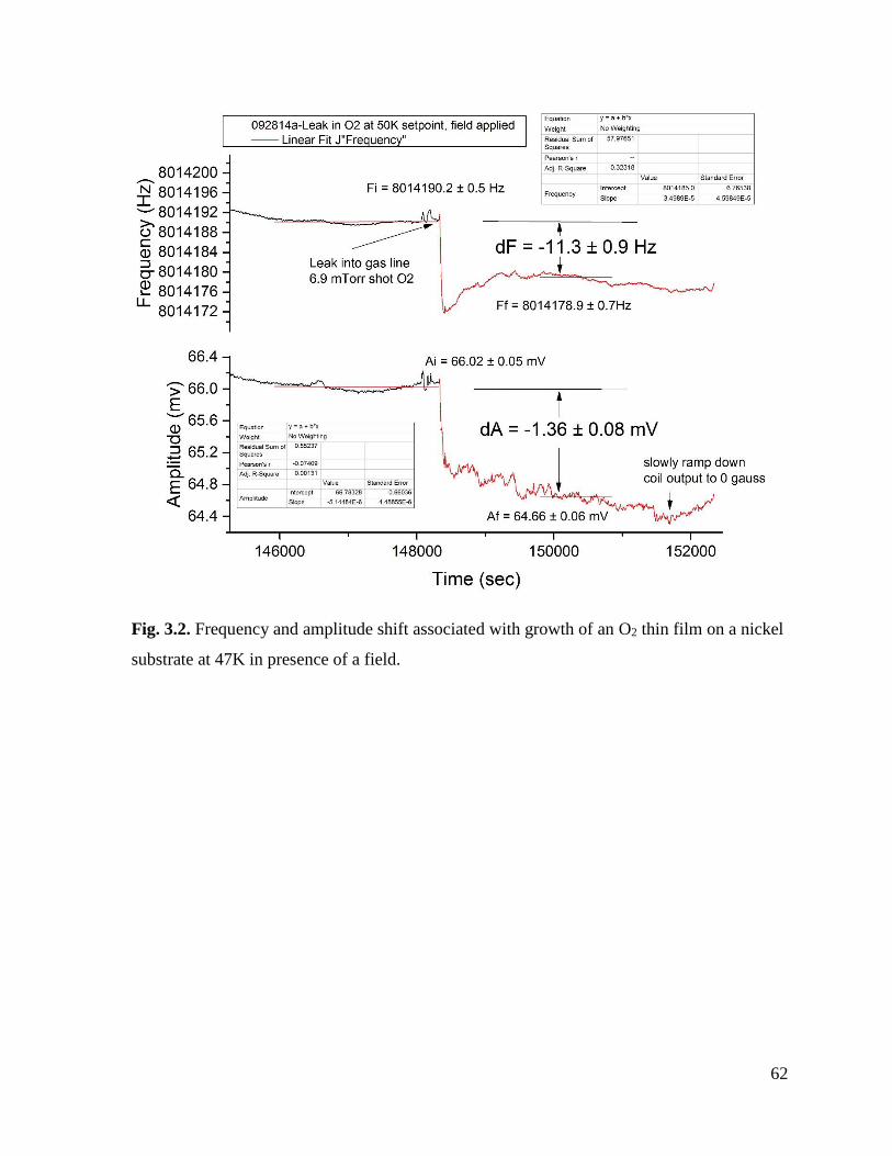
62

Fig. 3.2. Frequency and amplitude shift associated with growth of an O2 thin film on a nickel

substrate at 47K in presence of a field.

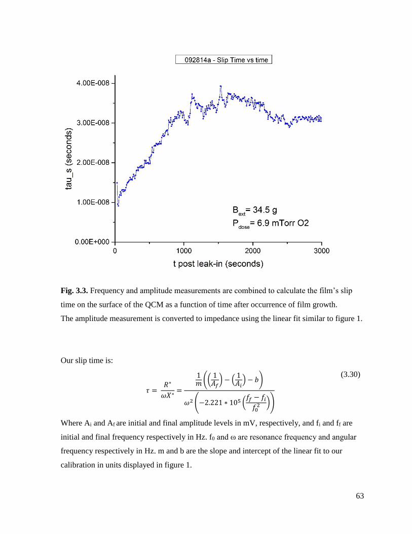
63

Fig. 3.3. Frequency and amplitude measurements are combined to calculate the film’s slip

time on the surface of the QCM as a function of time after occurrence of film growth.

The amplitude measurement is converted to impedance using the linear fit similar to figure 1.

Our slip time is:

𝜏 = 𝑅∗

𝜔𝑋∗=

1𝑚 ((

1𝐴𝑓

) − (1𝐴𝑖

) − 𝑏)

𝜔2 (−2.221 ∗ 105 (𝑓𝑓 − 𝑓𝑖

𝑓02 ))

(3.30)

Where Ai and Af are initial and final amplitude levels in mV, respectively, and fi and ff are

initial and final frequency respectively in Hz. f0 and ω are resonance frequency and angular

frequency respectively in Hz. m and b are the slope and intercept of the linear fit to our

calibration in units displayed in figure 1.

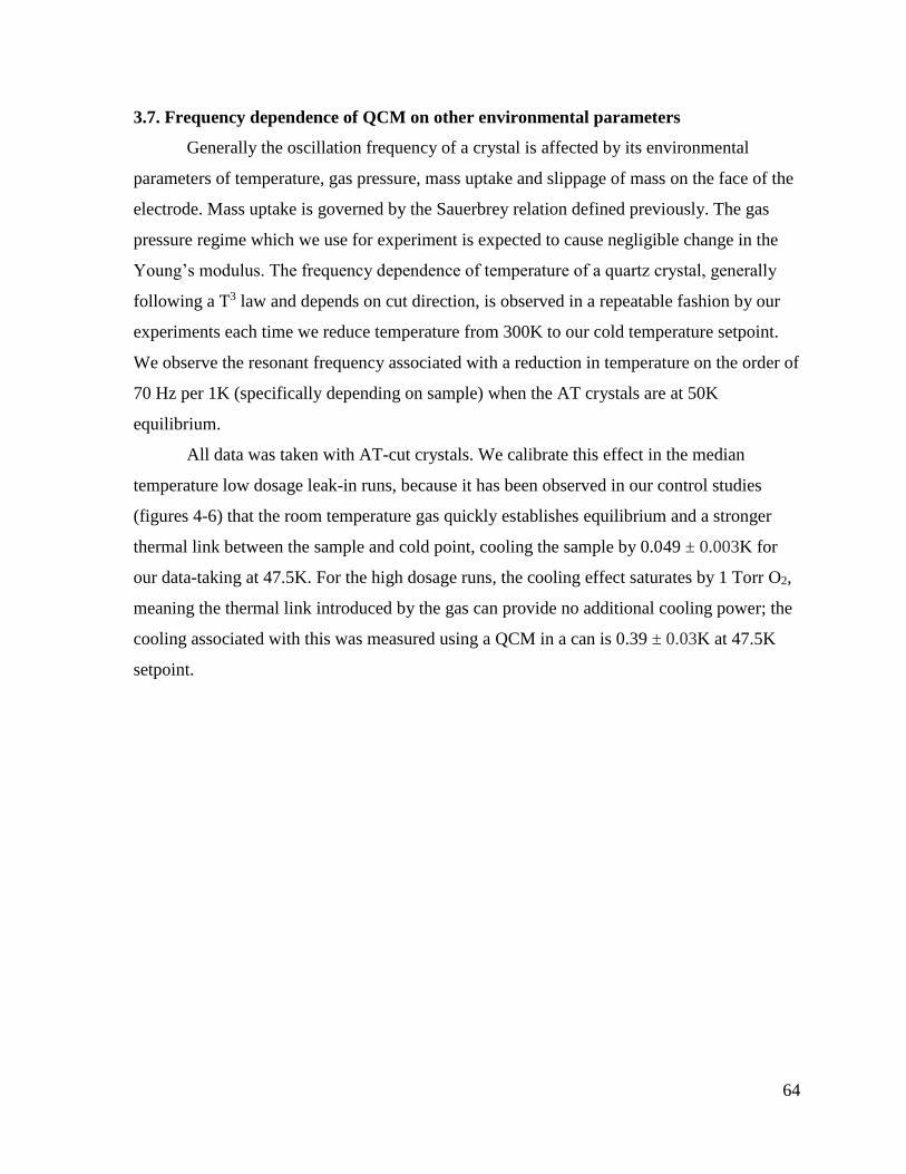
64

3.7. Frequency dependence of QCM on other environmental parameters

Generally the oscillation frequency of a crystal is affected by its environmental

parameters of temperature, gas pressure, mass uptake and slippage of mass on the face of the

electrode. Mass uptake is governed by the Sauerbrey relation defined previously. The gas

pressure regime which we use for experiment is expected to cause negligible change in the

Young’s modulus. The frequency dependence of temperature of a quartz crystal, generally

following a T3 law and depends on cut direction, is observed in a repeatable fashion by our

experiments each time we reduce temperature from 300K to our cold temperature setpoint.

We observe the resonant frequency associated with a reduction in temperature on the order of

70 Hz per 1K (specifically depending on sample) when the AT crystals are at 50K

equilibrium.

All data was taken with AT-cut crystals. We calibrate this effect in the median

temperature low dosage leak-in runs, because it has been observed in our control studies

(figures 4-6) that the room temperature gas quickly establishes equilibrium and a stronger

thermal link between the sample and cold point, cooling the sample by 0.049 ± 0.003K for

our data-taking at 47.5K. For the high dosage runs, the cooling effect saturates by 1 Torr O2,

meaning the thermal link introduced by the gas can provide no additional cooling power; the

cooling associated with this was measured using a QCM in a can is 0.39 ± 0.03K at 47.5K

setpoint.

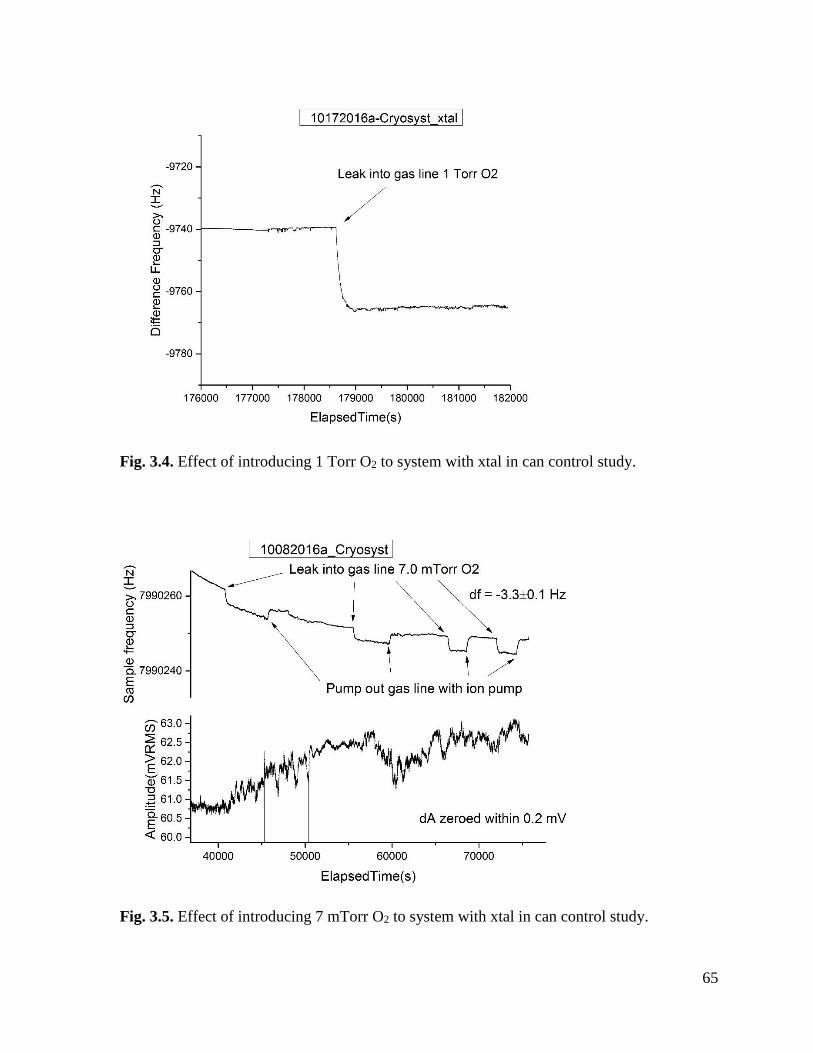
65

Fig. 3.4. Effect of introducing 1 Torr O2 to system with xtal in can control study.

Fig. 3.5. Effect of introducing 7 mTorr O2 to system with xtal in can control study.

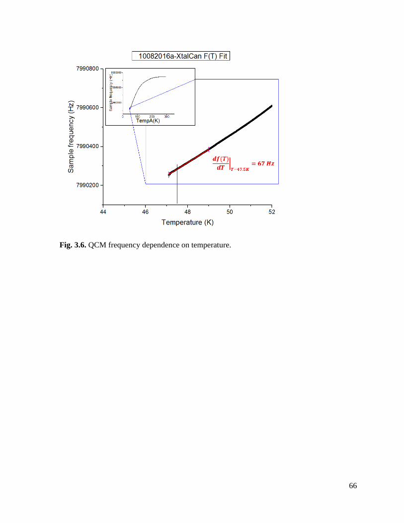
66

Fig. 3.6. QCM frequency dependence on temperature.

67

3.8. QCM frequency shift dependence on slippage of films

Mass attached to an oscillator’s face in a slippery fashion reduces the frequency shift

otherwise expected by the Sauerbrey relation, because the total film mass is not fully

registered. The equation used for this correction is:

𝜌2 =𝜌2𝑐

(1 + (𝜔𝜏)2) .

(3.31)

Where ρ2 is the coverage calculated in Eq. 3.13 and ρ2c is the corrected coverage. Generally

for films with slip time τ = 1 ns, the effect is negligible to within 1% of our observed values.

In some of our data the slip time is larger and we account for this slippage effect.

68

3.9. Correction to Measured Pressures due to thermal transpiration

Taking pressure measurements using a gauge at room temperature of closed system

involving a cold part of a vacuum system introduces the need for a correction due to

equilibrium gas flow in the absence of pressure gradients. This is an effect known as thermal

transpiration, and is used to correct our room temperature pressure gauge measurements of

the gas line system.

A convenient way to calculate the effect has been the derivation [8]:

1 − (𝑃1𝑃2

)

1 − (𝑇1𝑇2

)1/2=

1

𝛼𝑦2 + 𝛽𝑦 + 𝜇

(3.32)

Where P1 and P2

are the pressure at cold point and gauge pressure (Torr), and T1 and T2

are

the temperature at cold point and room temperature (K). α = π/128, β = π/12 and μ =

(1+gy)/(1+hy), and where a convenient way to calculate y is:

𝑦 =

𝑃2𝑑𝜎2

2.33 ∗ |𝑇|∗ 1000

(3.33)

Where d is the inner diameter of the tube (mm), |T| is average temperature between T1 and T2,

and 𝜎 is the molecular hard sphere diameter. Thus for our O2 leak-in runs of gauge reading 2

mTorr, the actual pressure in the vicinity of the cold tip is 5.7*10-4 Torr when the cold tip is

at 47K. Additionally, prior to leak-in our typical pressure readings of 2*10-9 Torr correspond

to a value of 8*10-10 Torr at the site of the cold tip, ensuring UHV conditions on the face of

our sample.

69

3.10. Experimental Hardware

The measurement of nanofriction between two bodies involves strict environmental

controls due to the delicate nature of the interface. Firstly the film must be at thermal

equilibrium and its composition known, as well as that of the substrate. Secondly interaction

of the film with gas-phase particles risks interruption of the measurement so typically it must

be done within ultra-high vacuum (UHV) conditions. For example, within one second at 10-6

Torr a film forms of about monolayer thickness assuming a sticking coefficient of unity. My

cryogenic experiment chamber has UHV, mTorr gas dosage, magnetic field control and low

temperature setpoint to within 0.01K specification capabilities.

3.11. Vacuum System

For the studies I designed and constructed a cryo system consisting of one vacuum

system contained within another separate vacuum system - the pressure of each can be

independently controlled (figure 7). The inner vacuum system consists of the gas line and the

sample cube and has UHV capability (figure 8). The outer system’s boundary is defined by

the shroud and is typically pumped to 10-6 Torr. The shroud contains the cold tip, heat bridge,

sample cube and gas line and radiation shield. Evacuation of both systems is conducted by

means of a turbomolecular pump - Pfeiffer Balzers model TPH-062 powered with Pfeiffer

Balzers TCP 121 turbo controller unit.

This turbo pump’s exhaust is connected to the intake of a cryosorption pump – a

stainless steel container filled with Xeolite powder and submerged in liquid nitrogen inside a

dewar. The

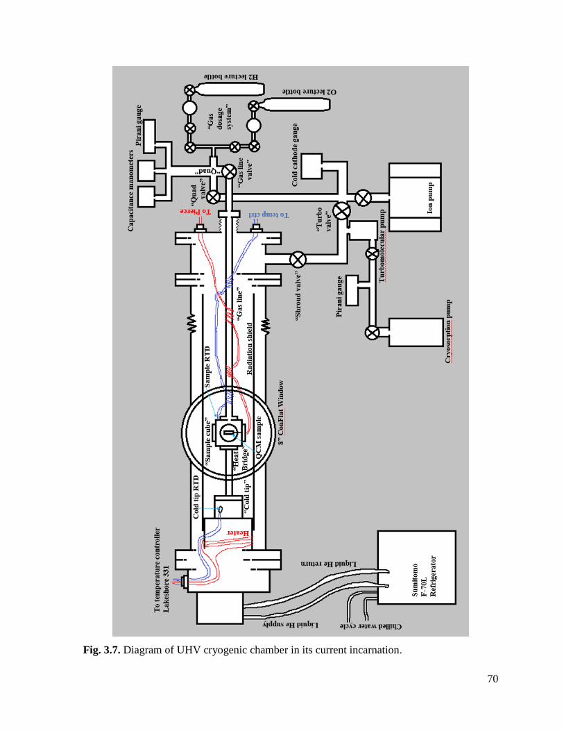
70

Fig. 3.7. Diagram of UHV cryogenic chamber in its current incarnation.

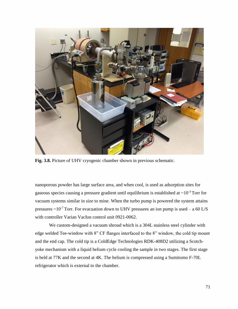
71

Fig. 3.8. Picture of UHV cryogenic chamber shown in previous schematic.

nanoporous powder has large surface area, and when cool, is used as adsorption sites for

gaseous species causing a pressure gradient until equilibrium is established at ~10-3 Torr for

vacuum systems similar in size to mine. When the turbo pump is powered the system attains

pressures ~10-7 Torr. For evacuation down to UHV pressures an ion pump is used – a 60 L/S

with controller Varian VacIon control unit 0921-0062.

We custom-designed a vacuum shroud which is a 304L stainless steel cylinder with

edge welded Tee-window with 8” CF flanges interfaced to the 8” window, the cold tip mount

and the end cap. The cold tip is a ColdEdge Technologies RDK-408D2 utilizing a Scotch-

yoke mechanism with a liquid helium cycle cooling the sample in two stages. The first stage

is held at 77K and the second at 4K. The helium is compressed using a Sumitomo F-70L

refrigerator which is external to the chamber.

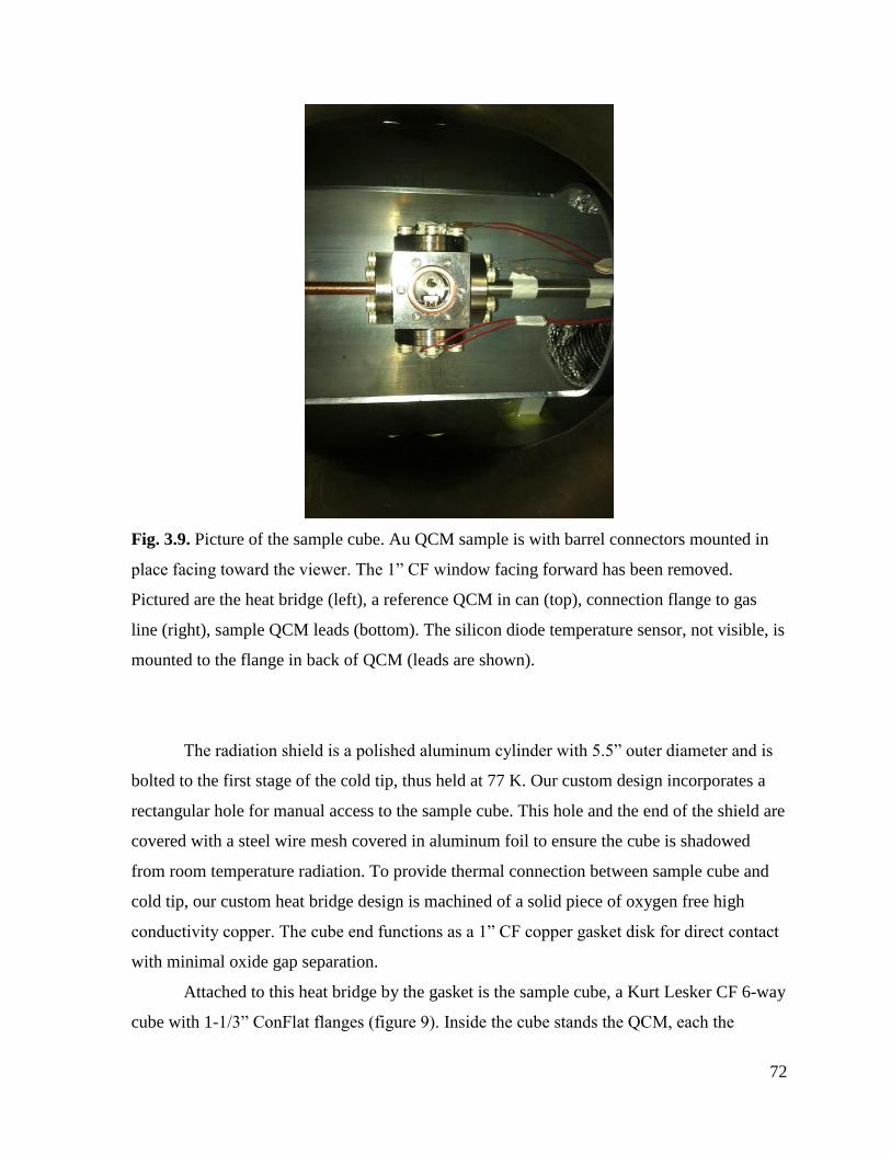
72

Fig. 3.9. Picture of the sample cube. Au QCM sample is with barrel connectors mounted in

place facing toward the viewer. The 1” CF window facing forward has been removed.

Pictured are the heat bridge (left), a reference QCM in can (top), connection flange to gas

line (right), sample QCM leads (bottom). The silicon diode temperature sensor, not visible, is

mounted to the flange in back of QCM (leads are shown).

The radiation shield is a polished aluminum cylinder with 5.5” outer diameter and is

bolted to the first stage of the cold tip, thus held at 77 K. Our custom design incorporates a

rectangular hole for manual access to the sample cube. This hole and the end of the shield are

covered with a steel wire mesh covered in aluminum foil to ensure the cube is shadowed

from room temperature radiation. To provide thermal connection between sample cube and

cold tip, our custom heat bridge design is machined of a solid piece of oxygen free high

conductivity copper. The cube end functions as a 1” CF copper gasket disk for direct contact

with minimal oxide gap separation.

Attached to this heat bridge by the gasket is the sample cube, a Kurt Lesker CF 6-way

cube with 1-1/3” ConFlat flanges (figure 9). Inside the cube stands the QCM, each the

73

electrical leads of which is mounted by means of a barrel pin to a pin of a Kurt Lesker 1.33”

2-pin power feedthrough. The cube’s other faces have been functionalized with flanges with

a 8 MHz reference QCM in a can, a gas line, a temperature sensor, and a 1.33” window

flange. The gas line is a stainless steel thin-walled tube with 3/8” outer diameter.

Temperature measurement at

the cube is done with LakeShore DT-670 SD silicon diode which has been secured to the

cube’s rear flange by means of a bolt screwed into a tapped hole sandwiching the diode and

thermally anchored with a short length of indium solder wire.

The electrical leads of the sample QCM, the temperature sensor, and the reference

QCM are soldered to lengths of constantan wire - Omega Engineering TFCC-015 - which is

Teflon-coated (red in color). These leads extend down the gas line, and are wrapped around it

at two intervals each for the purpose of thermal anchoring. Glass cloth tape of 3M 27 Model

16007 is used at several points within the shroud to attach leads to their desired positions

within the shroud and in the vicinity of the cube. At the opposite end of the chamber (near

the gas dosage system) the leads terminate at soldered joints at two separate feedthroughs.

On the external side of the feedthroughs, the sample QCM’s leads extend from the

feedthrough to the isolation box and are attached into the Pierce circuitry (figure 10), and the

temperature detector’s leads are attached into the back of the LakeShore 331 temperature

controller.

The Peirce oscillator circuit drives the QCM at its resonance frequency and has

output frequency signal is mixed with a reference signal supplied by an 8 MHz can crystal

driven by a separate Pierce circuit. The Mixed signal is run through a low-pass filter and

detected using an Agilent 53181a frequency counter. The amplitude was measured by using a

Keithley 2000 multimeter in AC amplitude measurement mode. The circuits were powered

by a Viz/Kappa WP-773 DC power supply. I have drawn a diagram of the circuit, reproduced

below. The Pierce circuit operates well in the presence of high stray capacitances and has

high frequency stability [9]. A mixer circuit in figure 11 is reproduced from [9].

The gas dosage system sits at the opposite end of the gas line from the cube (figure

12). Its structure comprises the “quad”: a Kurt Lesker 4-way standard cross. Attached to the

top are pressure gauges; the right has Swagelok components connecting the quad to lecture

74

bottles of 99.999% pure oxygen, 99.999% pure nitrogen, and 99.999% pure He – dependent

upon which

Figure. 3.10. Schematic of Pierce oscillator circuitry. Two identical boards are used – one

tuned to the resonance conditions of the sample QCM, and another separate board for the

reference crystal. Adapted from [11].

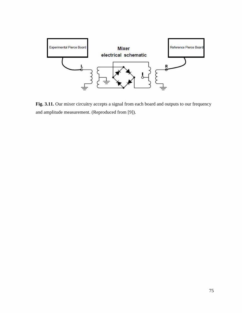
75

Fig. 3.11. Our mixer circuitry accepts a signal from each board and outputs to our frequency

and amplitude measurement. (Reproduced from [9]).

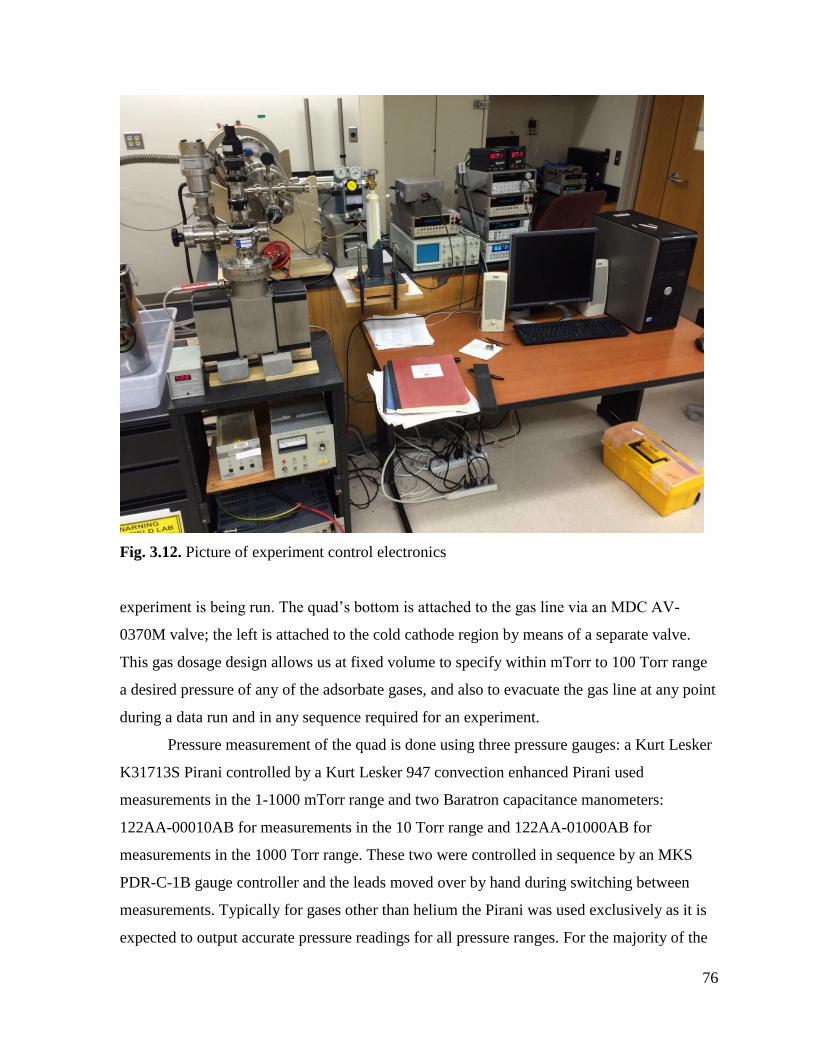
76

Fig. 3.12. Picture of experiment control electronics

experiment is being run. The quad’s bottom is attached to the gas line via an MDC AV-

0370M valve; the left is attached to the cold cathode region by means of a separate valve.

This gas dosage design allows us at fixed volume to specify within mTorr to 100 Torr range

a desired pressure of any of the adsorbate gases, and also to evacuate the gas line at any point

during a data run and in any sequence required for an experiment.

Pressure measurement of the quad is done using three pressure gauges: a Kurt Lesker

K31713S Pirani controlled by a Kurt Lesker 947 convection enhanced Pirani used

measurements in the 1-1000 mTorr range and two Baratron capacitance manometers:

122AA-00010AB for measurements in the 10 Torr range and 122AA-01000AB for

measurements in the 1000 Torr range. These two were controlled in sequence by an MKS

PDR-C-1B gauge controller and the leads moved over by hand during switching between

measurements. Typically for gases other than helium the Pirani was used exclusively as it is

expected to output accurate pressure readings for all pressure ranges. For the majority of the

77

experiments making up this thesis the pressure readings were handwritten directly to my lab

notebook.

The magnetic field control system consists of an electromagnet and its controller - a

GMW 5451 outputting 0.77 mT/A using current controller Kepco BP-20-20M. The

electromagnet is placed so that the shroud goes through the center – as such the fields

produced point in a direction parallel or anti-parallel with the axis of the vacuum shroud. The

measurements of frequency, amplitude, time, coil current, and pressure are recorded in a

LabVIEW program figure 17 – the data levels of which are recorded once every five seconds.

A schematic of the data recording process is presented in figure 15.

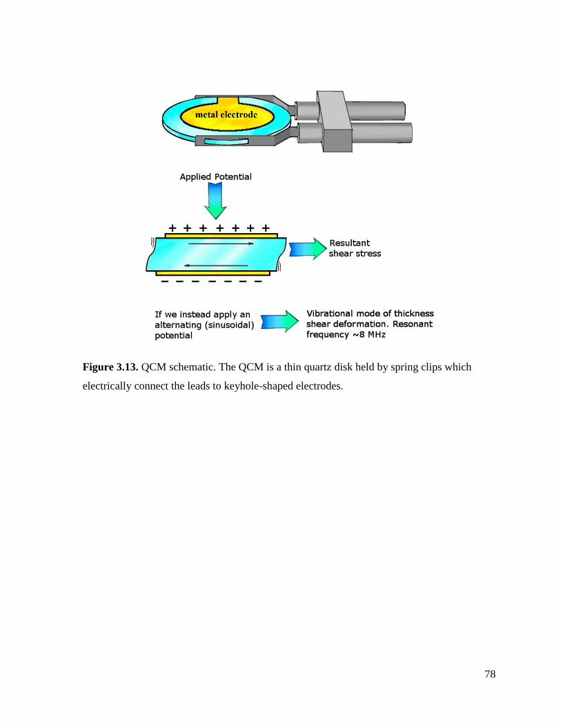
78

Figure 3.13. QCM schematic. The QCM is a thin quartz disk held by spring clips which

electrically connect the leads to keyhole-shaped electrodes.

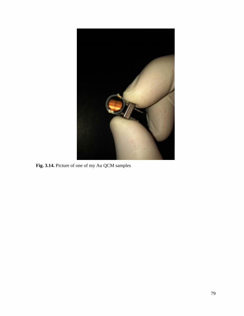
79

Fig. 3.14. Picture of one of my Au QCM samples

80

3.12. Sample Fabrication

Our studies use three QCM samples: Ni/Ni which has a nickel electrode on each side,

Au/Au which has a gold electrode on each side, and Fe-Bipy/Au which has two gold

electrodes, one of which has 100nm thick Fe-Bipy film grown atop it. In this section we

detail how we fabricated the Ni sample as well as the Fe-Bipy/Au sample. The Au sample

was purchased through

3.13. Ni/Ni QCM sample

To fabricate our Ni sample, we start with a blank quartz disk and finish with a Ni

electrode QCM mounted in the UHV chamber. Below are details of the entire process

featuring e-beam evaporation in a separate chamber.

Our cleaning procedure [10] is to wash the QCM blank crystal in running water, rinse

with de-ionized water, immerse in 0.05 M NaOH solution for about 30 minutes, let dry in air,

treat in a UV-ozone cleaner for 30 minutes on each side, immerse in ethanol for about 30

minutes, let dry again, and then treat each side in UV-ozone for 30 minutes again.

The sample is then loaded into a tab chamber for deposition. The crystal is held

between two flat stainless steel plates that act as masks by obscuring both faces of the crystal.

There are machined crescent-shaped holes in the mask. The masked crystal is placed within

the chamber above a Ti sublimation coil which is used as the source of deposition, and the

chamber is pumped down to 10−7 Torr. When this base pressure is reached, an alternating

current of near 60 A is driven through the coil, heating it to evaporation temperature and

growing a 230 nm Ti film on the crystal in the shape of a crescent on each edge.

The crystal is then removed from the tab chamber and is then placed into a connector

armature using Ted Pella conductive silver 187 Ag paint and then the connector is cemented

into place inside the stainless steel holder mask (figure 14) using Omega CC high temp

cement. The mask allows in situ manipulation of the sample within a vacuum chamber,

protects it and allows us to grow electrodes of the specified shape. To cure the cement, the

sample is then baked for 3 hours in a vacuum oven at 150C.

The sample is then placed inside a deposition chamber (figure 16) and the pressure is

reduced to 10−8 Torr. Ni electrodes of 30 nm are deposited at 0.1 nm/minute by means of a

Tungsten filament e-beam gun targeted upon a Ni rod held at 4.2 kV. A current of 6 A causes

81

the filament to thermionically emit electrons which are captured into the rod, causing it to

glow red hot and heating it to melting. Ni atoms are evaporated in a path from this source

onto the sample’s face, between which intervenes the stainless steel mask allowing for

electrode ‘keyhole’ shape specification. The sample is then transferred in situ to a ceramic

heater and warmed to 200 C under 10−10 Torr.

3.14. Au/Au QCM sample

The 8 MHz Au QCMs purchased from Laptech Precision Inc. [3] were AT-cut and

0.375 inches in diameter with a keyhole design with a diameter of 0.250 inches made from

gold deposited atop a thin chrome adhesion layer and optically polished. It is placed in a

sample holder equivalent to that described above and electrically connected into place using

Ag paint.

3.15. Fe-Bipy/Au QCM sample

To fabricate our Bipy/Au-1s-B sample, we placed an Au/Au sample QCM (equivalent

to the one described above) into a Knudson cell. The chamber was evacuated to 10-7 Torr by

means of a turbomolecular Pfeiffer pump and a 100 nm thick film of “Bipy” material

Fe[(H2Bpz2)2bpy]was deposited at a rate of 0.1 nm/s by means of heating a tungsten wire

wrapped around a quartz crucible containing the material. The material was fabricated in a

procedure previously described [11]. One side of the QCM was coated with the material - the

opposite face remained as an Au electrode as a means to study two separate diamagnetic

systems simultaneously. These films on Au(111) have been shown to undergo a molecular

spin-crossover transition at 140K [12] but for our low temperature experiments they’re

considered as a diamagnetic material (expected below transition temperature 140 K). The

purple compound was observed to undergo a spin-crossover transition by means of cooling a

similarly grown film on Al foil and submerging in liquid N2.

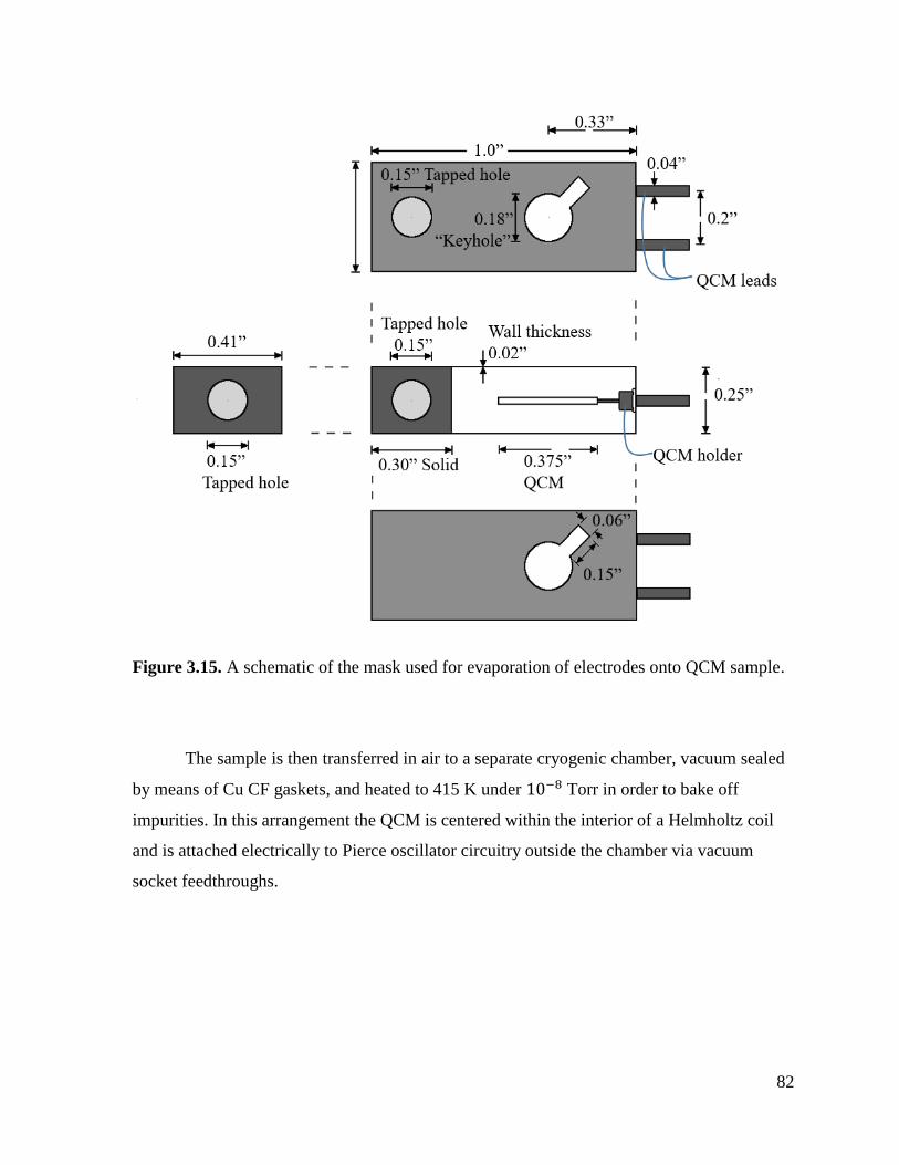
82

Figure 3.15. A schematic of the mask used for evaporation of electrodes onto QCM sample.

The sample is then transferred in air to a separate cryogenic chamber, vacuum sealed

by means of Cu CF gaskets, and heated to 415 K under 10−8 Torr in order to bake off

impurities. In this arrangement the QCM is centered within the interior of a Helmholtz coil

and is attached electrically to Pierce oscillator circuitry outside the chamber via vacuum

socket feedthroughs.

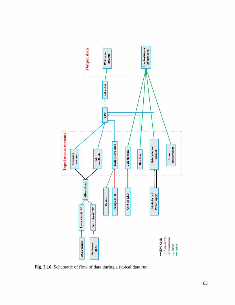
83

Fig. 3.16. Schematic of flow of data during a typical data run.

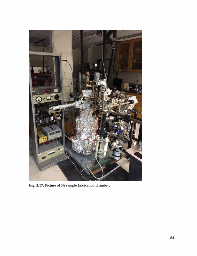
84

Fig. 3.17. Picture of Ni sample fabrication chamber.

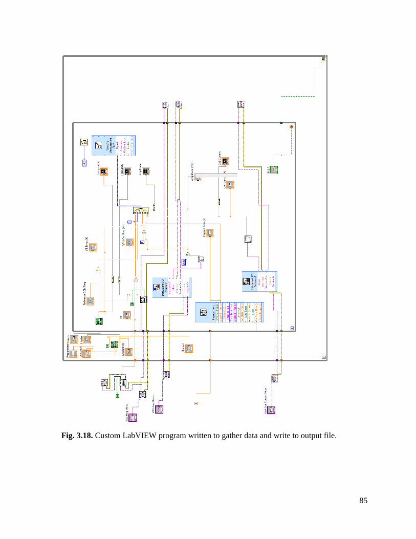
85

Fig. 3.18. Custom LabVIEW program written to gather data and write to output file.

86

REFERENCES CHAPTER 3

[1] Krim, J., & Widom, A. (1988). Damping of a crystal oscillator by an adsorbed monolayer

and its relation to interfacial viscosity. Physical Review B, 38(17), 184–189.

[2] Montagut, Y., Narbon, J.G., Jimenez, Y., March C., Montoya, A., & Arnau, A. (2011).

QCM Technology in Biosensors, Biosensors - Emerging Materials and Applications, Prof.

Pier Andrea Serra (Ed.), InTech, DOI: 10.5772/17991.

[3] Laptech Precision Inc., Part # XL1018, http://www.laptech.com.

[4] Sauerbrey, G. (1959). Verwendung von Schwingquarzen zur Wägung dünner Schichten

und zur Mikrowägung. Zeitschrift Für Physik, 155, 206–222.

http://doi.org/10.1007/BF01337937

[5] Highland, M., & Krim, J. (2006). Superconductivity Dependent Friction of Water,

Nitrogen, and Superheated He Films Adsorbed on Pb(111). Physical Review Letters,

96(June), 226107. http://doi.org/10.1103/PhysRevLett.96.226107

[6] Coffey, T., & Krim, J. (2005). Impact of substrate corrugation on the sliding friction

levels of adsorbed films. Physical Review Letters, 95(August), 1–4.

http://doi.org/10.1103/PhysRevLett.95.076101

[7] Coffey, T. S. (2004). Nanotribology Fundamentals: Predicting the viscous coefficient of

friction. (Doctoral dissertation). Retrieved from:

https://repository.lib.ncsu.edu/handle/1840.16/4149

[8] Miller, G. (1963). On the calculation of thermal transpiration. Journal of Physical

Chemistry, 67 (6) 1359-1361

[9] Lynch, I. I. (2011). Friction and Sliding of Polystyrene Micro Particles in the Presence

and Absence of Capillary Adhesion. (Doctoral dissertation). Retrieved from:

https://repository.lib.ncsu.edu/handle/1840.16/7338

87

[10] Hussain, Y., Krim, J., & Grant, C. (2005). OTS adsorption: A dynamic QCM study.

Colloids and Surfaces A: Physicochemical and Engineering Aspects, 262, 81–86.

http://doi.org/10.1016/j.colsurfa.2005.03.016

[11] Real, J. A., Muñoz, M. C., Faus, J., & Solans, X. (1997). Spin Crossover in Novel

Dihydrobis(1-pyrazolyl)borate [H2B(pz)2]-Containing Iron(II) Complexes. Synthesis, X-ray

Structure, and Magnetic Properties of [FeL{H2B(pz)2}2] (L = 1,10-Phenanthroline and 2,2‘-

Bipyridine). Inorganic Chemistry, 36(II), 3008–3013. http://doi.org/10.1021/ic960965c

[12] Pronschinske, A., Chen, Y., Lewis, G. F., Shultz, D. a., Calzolari, A., Buongiorno

Nardelli, M., & Dougherty, D. B. (2013). Modification of molecular spin crossover in

ultrathin films. Nano Letters, 13, 1429–1434. http://doi.org/10.1021/nl304304e

88

CHAPTER 4: RESULTS AND DISCUSSION OF O2 FILM GROWTH ON NI AT 47K

IN PRESENCE AND ABSENCE OF FIELD

4.1 Introduction

I present in the following chapters the results of my experiments measuring uptake of

oxygen and nitrogen films condensed on substrates of varying magnetic types. Experiments

were conducted at UHV conditions within the gas dosage system, a complete description of

which is in chapter 3. Generally the procedure was, after calibrating the QCM at room

temperature, the sample was cooled under vacuum, starting at room temperature, to a setpoint

such as 50K over the course of 8-10 hours. Materials we used for substrates are the

previously described QCM with both electrodes composed of nickel (Ni/Ni), a QCM with Au

electrodes on both sides (Au/Au), and the QCM sample with one side Fe-Bipy film on Au

and the other side Au (which we refer to as Bipy/Au-1s-B). We varied many of the

experimental parameters including temperature setpoint in the range 30K – 60K, applied

field strength value during film growth from 0 -34.5 gauss, magnetic on/off sequences with

film present, dosage pressure from 7 mTorr to 10 Torr and thus film thickness, and dosage

gas type O2 and N2.

This chapter is broken into sections based on which experiments were conducted. In

section 4.2 we first describe observations of the thick and thin film growth of O2 on a Ni

substrate at 47K, then magnetic field on/off sequences on such films in section 4.3. Then in

4.4 we discuss the candidate magnetic dissipation mechanisms at play which could explain

these results. Then, with aim to filter which mechanisms were active, we began experiments

in which we incrementally reduced the temperature, from 47.5 K to 27K, of thin O2 films

grown on the same Ni substrate in the absence of field; these results are presented in Chapter

5.

89

4.2 Results of experiments on growth of O2 films of varying thickness sliding on Ni in

the presence vs absence of applied field at 47K

In the following pages are data runs in which we grew O2 films of varying

thicknesses atop a nickel substrate. Film growth was conducted at a temperature of 47 K by

dosage of varying amounts of O2 gas into the vacuum chamber. We control the film thickness

by means of varying O2 dosage pressure between 1 Torr down to 7 mTorr, finding about

monolayer coverage at the 6 mTorr dosage levels.

A homogenous time-constant magnetic field of strength 34.5 gauss was either present

or absent during film growth for each run. The field’s spatial gradient is set to zero at the

location of the sample. When the O2 film is present and has established equilibrium, we

apply and remove the external B field in a magnet power on/off sequence. The field ramp-up

is done adiabatically over the course of 40s at a maximum rate of 1g/s in order to minimize

Lenz-law effects in the system. Films typically exhibited sliding, although occasional pinning

behavior is observed.

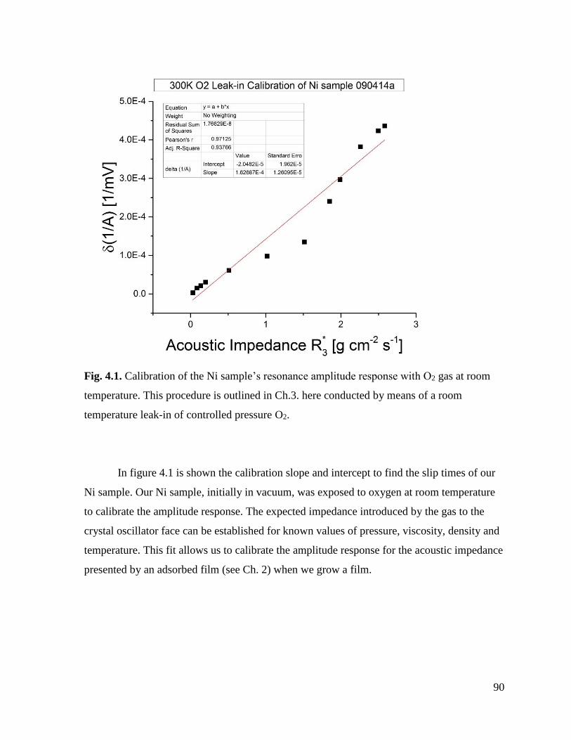
90

Fig. 4.1. Calibration of the Ni sample’s resonance amplitude response with O2 gas at room

temperature. This procedure is outlined in Ch.3. here conducted by means of a room

temperature leak-in of controlled pressure O2.

In figure 4.1 is shown the calibration slope and intercept to find the slip times of our

Ni sample. Our Ni sample, initially in vacuum, was exposed to oxygen at room temperature

to calibrate the amplitude response. The expected impedance introduced by the gas to the

crystal oscillator face can be established for known values of pressure, viscosity, density and

temperature. This fit allows us to calibrate the amplitude response for the acoustic impedance

presented by an adsorbed film (see Ch. 2) when we grow a film.

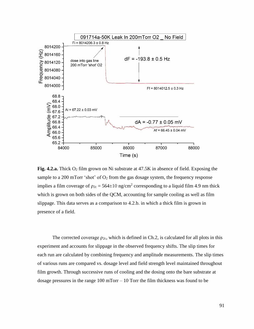
91

Fig. 4.2.a. Thick O2 film grown on Ni substrate at 47.5K in absence of field. Exposing the

sample to a 200 mTorr ‘shot’ of O2 from the gas dosage system, the frequency response

implies a film coverage of ρ2c = 564±10 ng/cm2 corresponding to a liquid film 4.9 nm thick

which is grown on both sides of the QCM, accounting for sample cooling as well as film

slippage. This data serves as a comparison to 4.2.b. in which a thick film is grown in

presence of a field.

The corrected coverage ρ2c, which is defined in Ch.2, is calculated for all plots in this

experiment and accounts for slippage in the observed frequency shifts. The slip times for

each run are calculated by combining frequency and amplitude measurements. The slip times

of various runs are compared vs. dosage level and field strength level maintained throughout

film growth. Through successive runs of cooling and the dosing onto the bare substrate at

dosage pressures in the range 100 mTorr – 10 Torr the film thickness was found to be

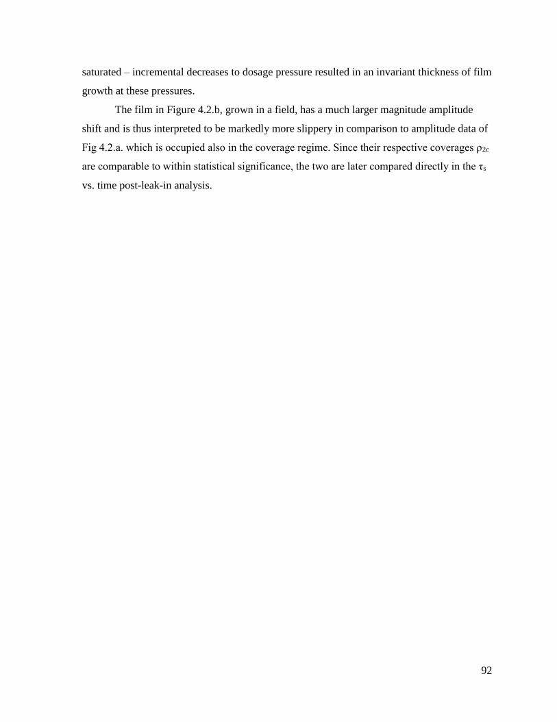
92

saturated – incremental decreases to dosage pressure resulted in an invariant thickness of film

growth at these pressures.

The film in Figure 4.2.b, grown in a field, has a much larger magnitude amplitude

shift and is thus interpreted to be markedly more slippery in comparison to amplitude data of

Fig 4.2.a. which is occupied also in the coverage regime. Since their respective coverages ρ2c

are comparable to within statistical significance, the two are later compared directly in the τs

vs. time post-leak-in analysis.

93

Figure 4.2.b Thick O2 film grown on Ni substrate at 47.5K in presence of field. Field

strength Bext = 34.5g is held constant while exposing the sample to a 100 mTorr ‘shot’ of O2

from the gas dosage system. The film’s coverage ρ2c = 585±11 ng/cm2 corresponds to a

liquid film 5.1 nm thick which is grown on each side of the QCM, accounting for sample

cooling as well as film slippage. The frequency shift is marginally larger, and amplitude shift

significantly larger, compared to data in Fig. 4.2.a, indicating the field causes a slippier film-

substrate interaction.

94

Fig. 4.3. Thick O2 films grown on Ni at 47.5 K in absence of field vs in presence of field.

Field absent case (upper graph) and presence of field (lower graph). Film coverages are

similar to the two previous runs: ρ2c =599±10 ng/cm2 (field absent) and 6.20±10 ng/cm2

(field present) respectively.

95

In Figure 4.3 are grown an O2 thick film on Ni in field condition absence (upper) and

presence (lower). The procedure for these runs was the exact same as the previous two

figures except in dosage level – here 10 Torr dosage pressure was used. The marginally

larger amplitude shift equilibrium level in the field presence data run indicates a longer slip

time. Film coverages are similar within the error bars of each, therefore these runs can be

compared in slip time analysis τs vs. time post-leak-in.

The frequency shift is relatively stable upon changes to the dosage level – this

indicates film dosage is saturated at this dosage level. It was found in successive data runs of

film growth that saturation occurs at about 50 mTorr O2 dosage pressure levels.

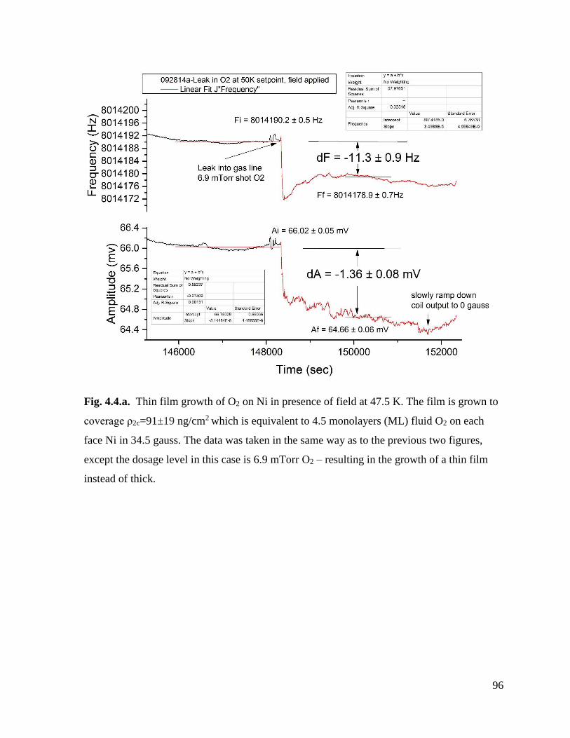
96

Fig. 4.4.a. Thin film growth of O2 on Ni in presence of field at 47.5 K. The film is grown to

coverage ρ2c=91±19 ng/cm2 which is equivalent to 4.5 monolayers (ML) fluid O2 on each

face Ni in 34.5 gauss. The data was taken in the same way as to the previous two figures,

except the dosage level in this case is 6.9 mTorr O2 – resulting in the growth of a thin film

instead of thick.

97

During the stability period in these runs, we study the effect on data levels of the

removal of field when the magnet coil supply is adiabatically ramped down. In the data run

in Fig. 4.4.a in the vicinity t=151700s (corresponding to tpl = 3300 s) over the course of 40 s,

a ramp-down was conducted from initial Bext = 34.5g to 0g; shortly thereafter occurs a

positive amplitude slope effect with time, indicating an increased level of friction upon field

removal for a film which was previously in equilibrium. The set of amplitude data within 300

s before this ramp-down is within one standard deviation of the post-ramp-down amplitude

data within 300 s so it is clear the effect on friction is not immediate.

The first time-derivative in amplitude undergoes a transition from general negative

pre-ramp-down towards positive slope upon removal of field. This is relatively subtle; it is

not immediately clear which is the correct procedure to quantify it, due to ambiguity of

which fit equation form is most valid during the ramp-down procedure; this would be

required to quantify the first time derivative as a function of tpl.

It is not known whether this amplitude upwards trend upon ramp-down is due to the

field or else due to the film establishing frictional equilibrium, however, we observe stability

in general for film growth runs within tpl < 1500 s; this implies the field ramp-down results in

a change in the film’s behavior, and that this change upon ramp-down is more subtle than the

effect of an equivalent field strength presence during film growth.

Again, in Fig.4.5, the amplitude slope increases after coil current ramp-down, again

in this run indicating a trend towards a new equilibrium increased level of friction upon field

removal. The set of amplitude data immediately before and after ramp-down - within 300 s -

are each within standard deviation of the opposing set; however, the general trend in

amplitude reverses from negative to positive upon field ramp-down. It is unclear if this

change in slope is due to the field removal or if the film had yet to fully establish equilibrium

within tpl = 2000 s. The film growths shown here are almost invariably stable, with standard

deviation in amplitude σAf < 0.1 mV low noise level over the time window 1500 s < tpl <

2500 s. This is evidence that the film’s frictional equilibrium state is slowly responding to the

reduction in field strength, as discussed in the preceding paragraphs.

The thin film frequency and amplitude data were least-squares fit to a linear trend for

all data taken in the time window -2400 s < tpl < 0 s (prior to the leak-in initiation). The initial

amplitude and frequency data are resolved to within a standard deviation, typical values σAi <

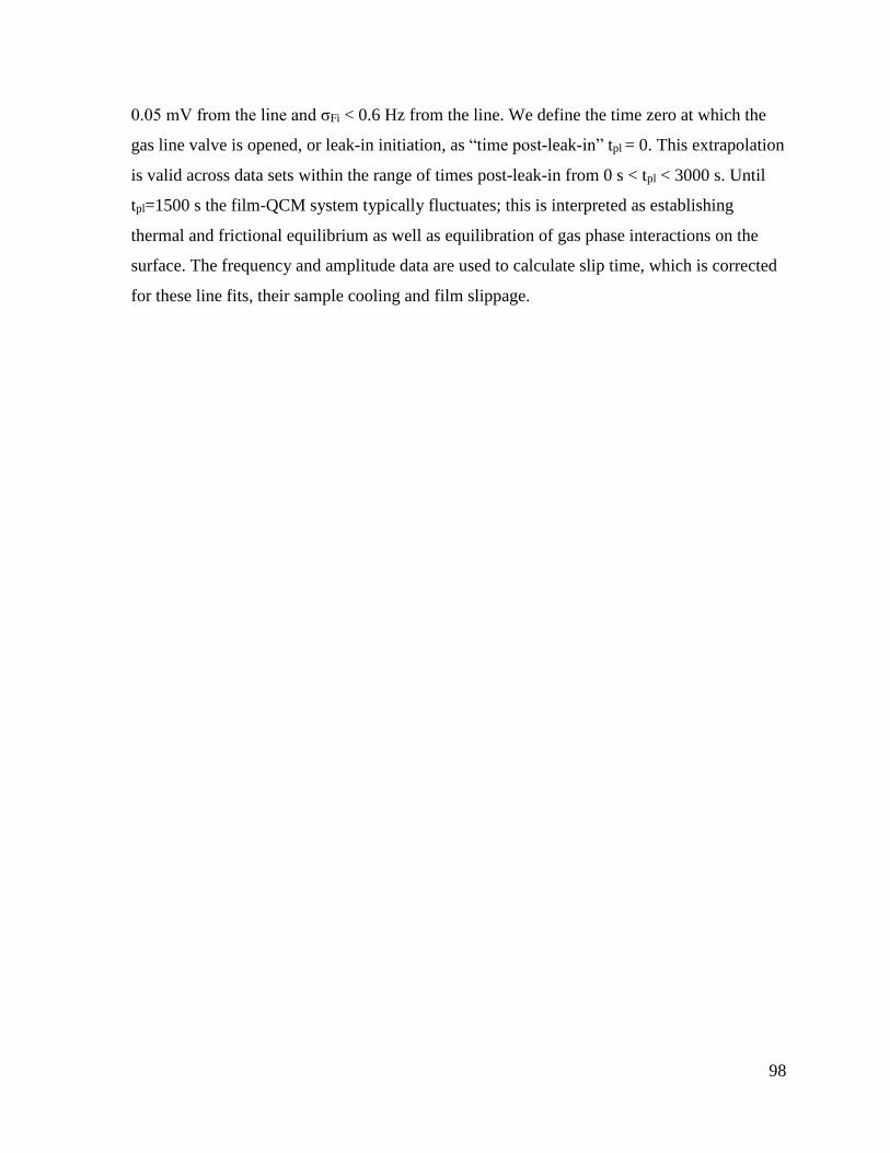
98

0.05 mV from the line and σFi < 0.6 Hz from the line. We define the time zero at which the

gas line valve is opened, or leak-in initiation, as “time post-leak-in” tpl = 0. This extrapolation

is valid across data sets within the range of times post-leak-in from 0 s < tpl < 3000 s. Until

tpl=1500 s the film-QCM system typically fluctuates; this is interpreted as establishing

thermal and frictional equilibrium as well as equilibration of gas phase interactions on the

surface. The frequency and amplitude data are used to calculate slip time, which is corrected

for these line fits, their sample cooling and film slippage.

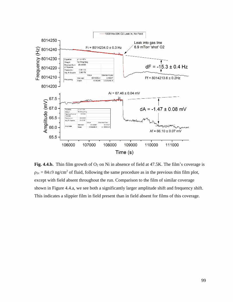
99

Fig. 4.4.b. Thin film growth of O2 on Ni in absence of field at 47.5K. The film’s coverage is

ρ2c = 84±9 ng/cm2 of fluid, following the same procedure as in the previous thin film plot,

except with field absent throughout the run. Comparison to the film of similar coverage

shown in Figure 4.4.a, we see both a significantly larger amplitude shift and frequency shift.

This indicates a slippier film in field present than in field absent for films of this coverage.

100

Fig. 4.5. Growth of O2 thin film on Ni substrate in presence of B field at 47.5 K. The film

growth proceeds to ρ2c = 90±13 ng/cm2 fluid film in Bext = 34.5 gauss. There are indications

of a response of film to removal of field – an increase in amplitude. This data run was

conducted in exact parallel with the data of the previous figures Fig 4.4.a and 4.4.b growing

thin films.

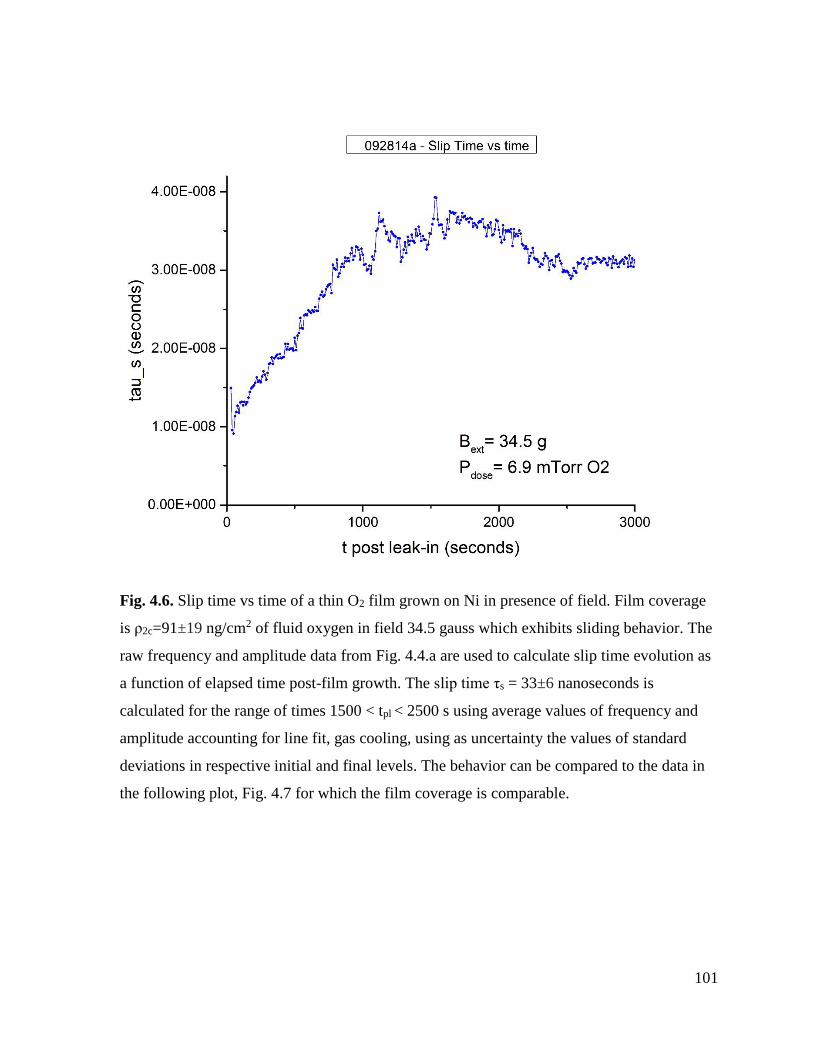
101

Fig. 4.6. Slip time vs time of a thin O2 film grown on Ni in presence of field. Film coverage

is ρ2c=91±19 ng/cm2 of fluid oxygen in field 34.5 gauss which exhibits sliding behavior. The

raw frequency and amplitude data from Fig. 4.4.a are used to calculate slip time evolution as

a function of elapsed time post-film growth. The slip time τs = 33±6 nanoseconds is

calculated for the range of times 1500 < tpl < 2500 s using average values of frequency and

amplitude accounting for line fit, gas cooling, using as uncertainty the values of standard

deviations in respective initial and final levels. The behavior can be compared to the data in

the following plot, Fig. 4.7 for which the film coverage is comparable.

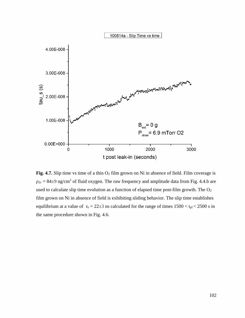
102

Fig. 4.7. Slip time vs time of a thin O2 film grown on Ni in absence of field. Film coverage is

ρ2c = 84±9 ng/cm2 of fluid oxygen. The raw frequency and amplitude data from Fig. 4.4.b are

used to calculate slip time evolution as a function of elapsed time post-film growth. The O2

film grown on Ni in absence of field is exhibiting sliding behavior. The slip time establishes

equilibrium at a value of τs = 22±3 ns calculated for the range of times 1500 < tpl < 2500 s in

the same procedure shown in Fig. 4.6.

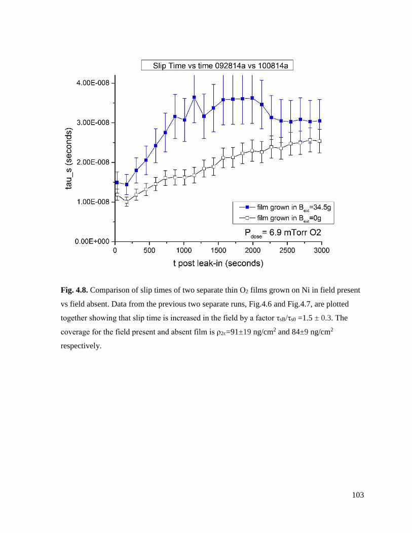
103

Fig. 4.8. Comparison of slip times of two separate thin O2 films grown on Ni in field present

vs field absent. Data from the previous two separate runs, Fig.4.6 and Fig.4.7, are plotted

together showing that slip time is increased in the field by a factor τsB/τs0 =1.5 ± 0.3. The

coverage for the field present and absent film is ρ2c=91±19 ng/cm2 and 84±9 ng/cm2

respectively.

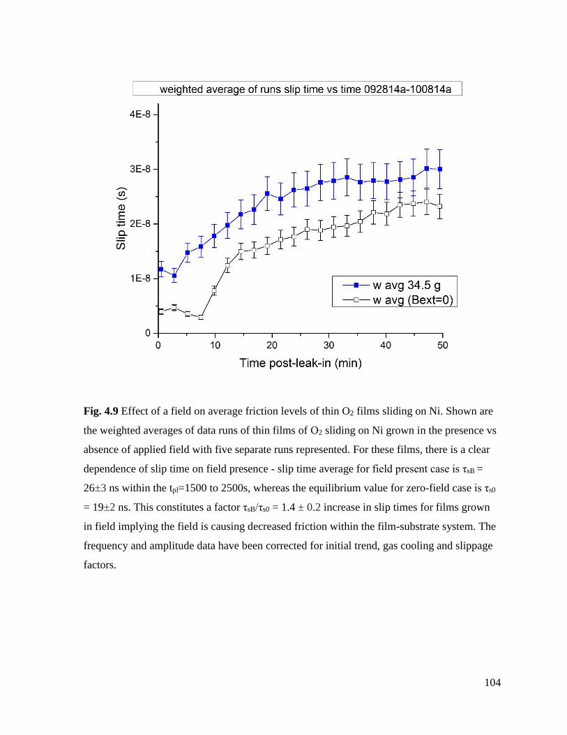
104

Fig. 4.9 Effect of a field on average friction levels of thin O2 films sliding on Ni. Shown are

the weighted averages of data runs of thin films of O2 sliding on Ni grown in the presence vs

absence of applied field with five separate runs represented. For these films, there is a clear

dependence of slip time on field presence - slip time average for field present case is τsB =

26±3 ns within the tpl=1500 to 2500s, whereas the equilibrium value for zero-field case is τs0

= 19±2 ns. This constitutes a factor τsB/τs0 = 1.4 ± 0.2 increase in slip times for films grown

in field implying the field is causing decreased friction within the film-substrate system. The

frequency and amplitude data have been corrected for initial trend, gas cooling and slippage

factors.

105

Fig. 4.10. Effect of a field on average friction levels of thin O2 films sliding on Ni for narrow

coverage window. Shown are the weighted averages of four separate data runs growing thin

films of coverages ρ2c=91±19 and ρ2c=90±14 ng/cm2 for the two field present cases, and for

the field absent case 84±9 ng/cm2 and ρ2c=75±8 ng/cm2.

106

Fig. 4.11. Slip time vs elapsed time of thick O2 films sliding on Ni in presence vs absence of

field. Film coverages for field present case are ρ2c=620±10 (run 2) and 585±11 ng/cm2 (run

4). Coverages for field absent runs are ρ2c=599±10 (run 1) and 564±10 ng/cm2 (run 3). The

raw frequency and amplitude data from Fig. 4.2.a, Fig. 4.2.b and Fig. 4.3 are used to

calculate slip time values for each data point. The O2 films grown on Ni in presence of field

are exhibiting decreased friction.

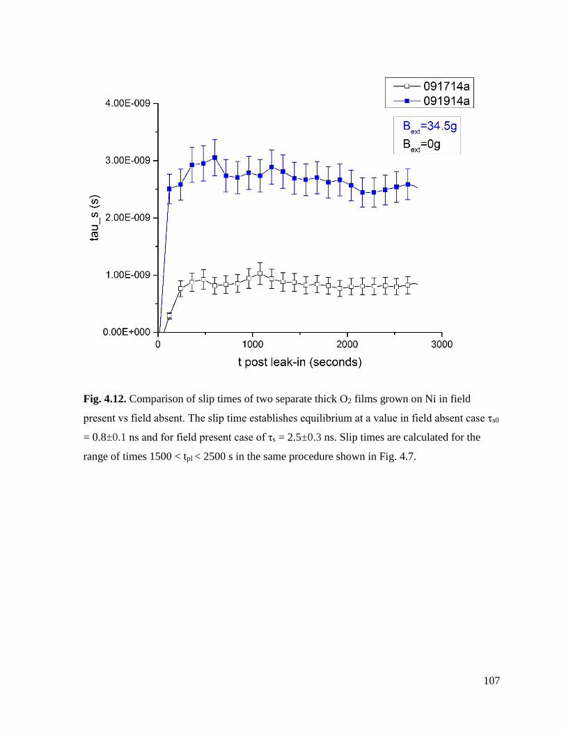
107

Fig. 4.12. Comparison of slip times of two separate thick O2 films grown on Ni in field

present vs field absent. The slip time establishes equilibrium at a value in field absent case τs0

= 0.8±0.1 ns and for field present case of τs = 2.5±0.3 ns. Slip times are calculated for the

range of times 1500 < tpl < 2500 s in the same procedure shown in Fig. 4.7.

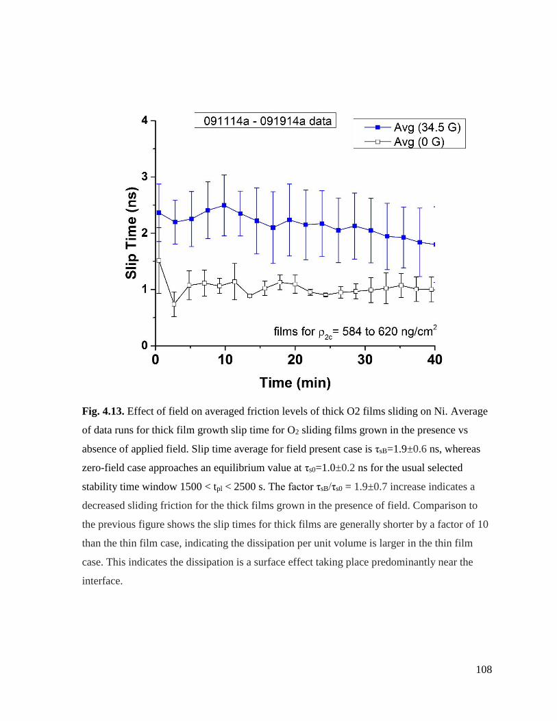
108

Fig. 4.13. Effect of field on averaged friction levels of thick O2 films sliding on Ni. Average

of data runs for thick film growth slip time for O2 sliding films grown in the presence vs

absence of applied field. Slip time average for field present case is τsB=1.9±0.6 ns, whereas

zero-field case approaches an equilibrium value at τs0=1.0±0.2 ns for the usual selected

stability time window 1500 < tpl < 2500 s. The factor τsB/τs0 = 1.9±0.7 increase indicates a

decreased sliding friction for the thick films grown in the presence of field. Comparison to

the previous figure shows the slip times for thick films are generally shorter by a factor of 10

than the thin film case, indicating the dissipation per unit volume is larger in the thin film

case. This indicates the dissipation is a surface effect taking place predominantly near the

interface.

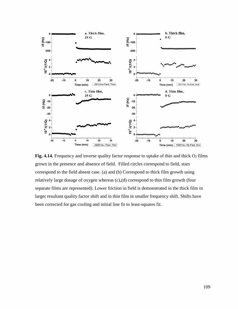
109

Fig. 4.14. Frequency and inverse quality factor response to uptake of thin and thick O2 films

grown in the presence and absence of field. Filled circles correspond to field, stars

correspond to the field absent case. (a) and (b) Correspond to thick film growth using

relatively large dosage of oxygen whereas (c),(d) correspond to thin film growth (four

separate films are represented). Lower friction in field is demonstrated in the thick film in

larger resultant quality factor shift and in thin film in smaller frequency shift. Shifts have

been corrected for gas cooling and initial line fit to least-squares fit.

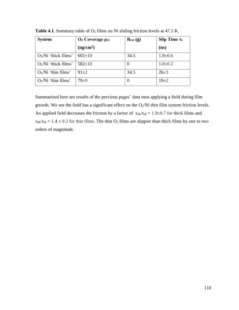
110

Table 4.1. Summary table of O2 films on Ni sliding friction levels at 47.5 K.

System O2 Coverage ρ2c

(ng/cm2)

Bext (g) Slip Time τs

(ns)

O2/Ni ‘thick films’ 602±10 34.5 1.9±0.6

O2/Ni ‘thick films’ 582±10 0 1.0±0.2

O2/Ni ‘thin films’ 91±2 34.5 26±3

O2/Ni ‘thin films’ 79±9 0 19±2

Summarized here are results of the previous pages’ data runs applying a field during film

growth. We see the field has a significant effect on the O2/Ni thin film system friction levels.

An applied field decreases the friction by a factor of τsB/τs0 = 1.9±0.7 for thick films and

τsB/τs0 = 1.4 ± 0.2 for thin films. The thin O2 films are slippier than thick films by one to two

orders of magnitude.

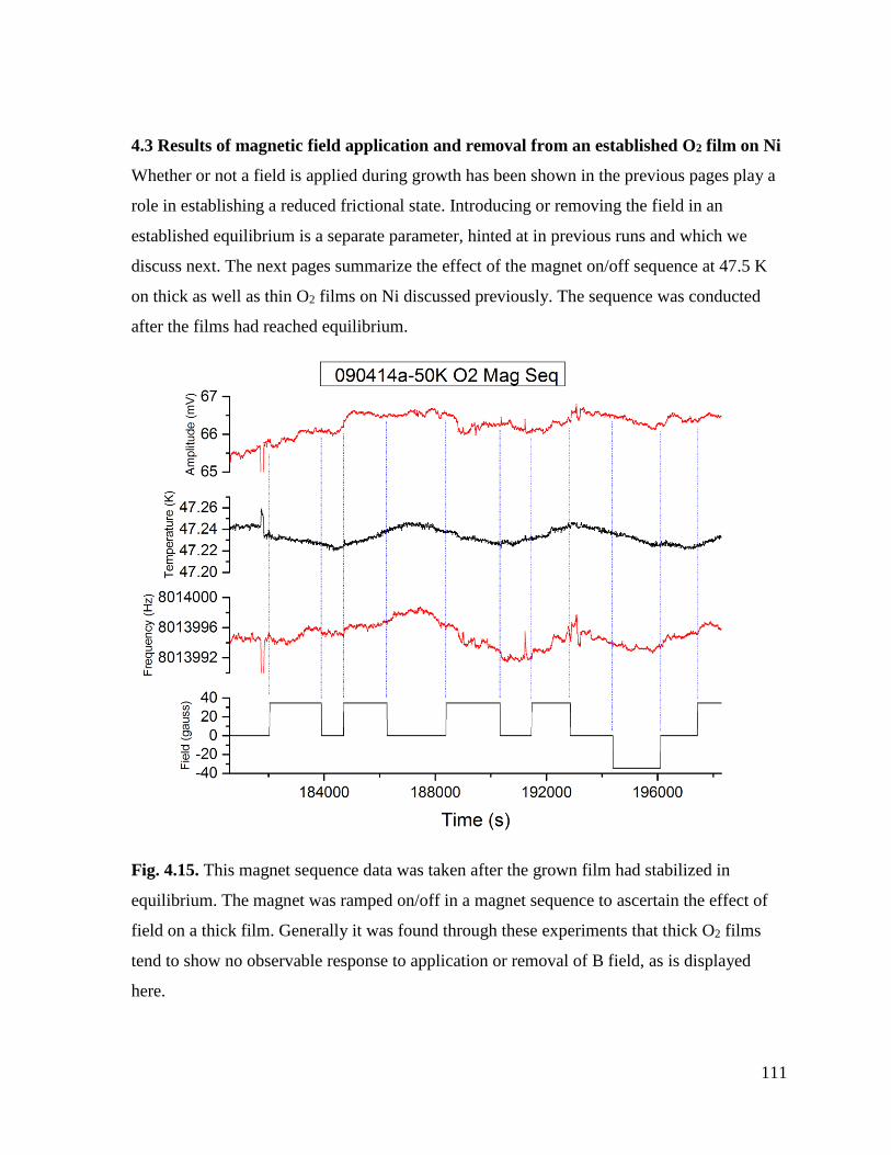
111

4.3 Results of magnetic field application and removal from an established O2 film on Ni

Whether or not a field is applied during growth has been shown in the previous pages play a

role in establishing a reduced frictional state. Introducing or removing the field in an

established equilibrium is a separate parameter, hinted at in previous runs and which we

discuss next. The next pages summarize the effect of the magnet on/off sequence at 47.5 K

on thick as well as thin O2 films on Ni discussed previously. The sequence was conducted

after the films had reached equilibrium.

Fig. 4.15. This magnet sequence data was taken after the grown film had stabilized in

equilibrium. The magnet was ramped on/off in a magnet sequence to ascertain the effect of

field on a thick film. Generally it was found through these experiments that thick O2 films

tend to show no observable response to application or removal of B field, as is displayed

here.

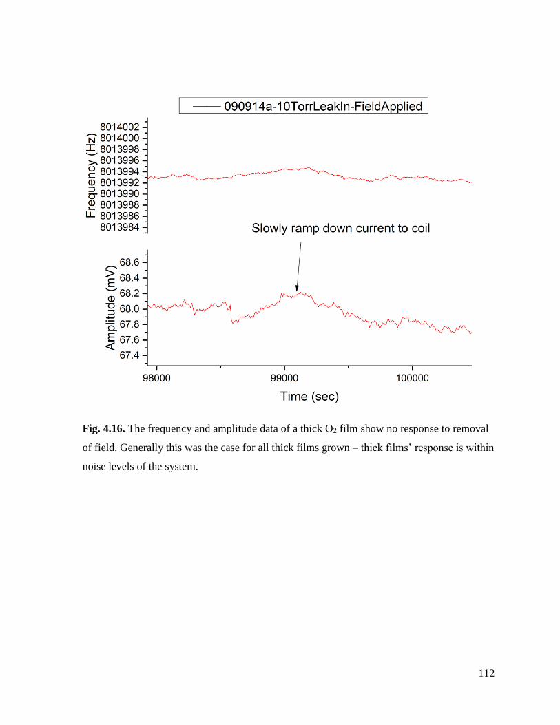
112

Fig. 4.16. The frequency and amplitude data of a thick O2 film show no response to removal

of field. Generally this was the case for all thick films grown – thick films’ response is within

noise levels of the system.

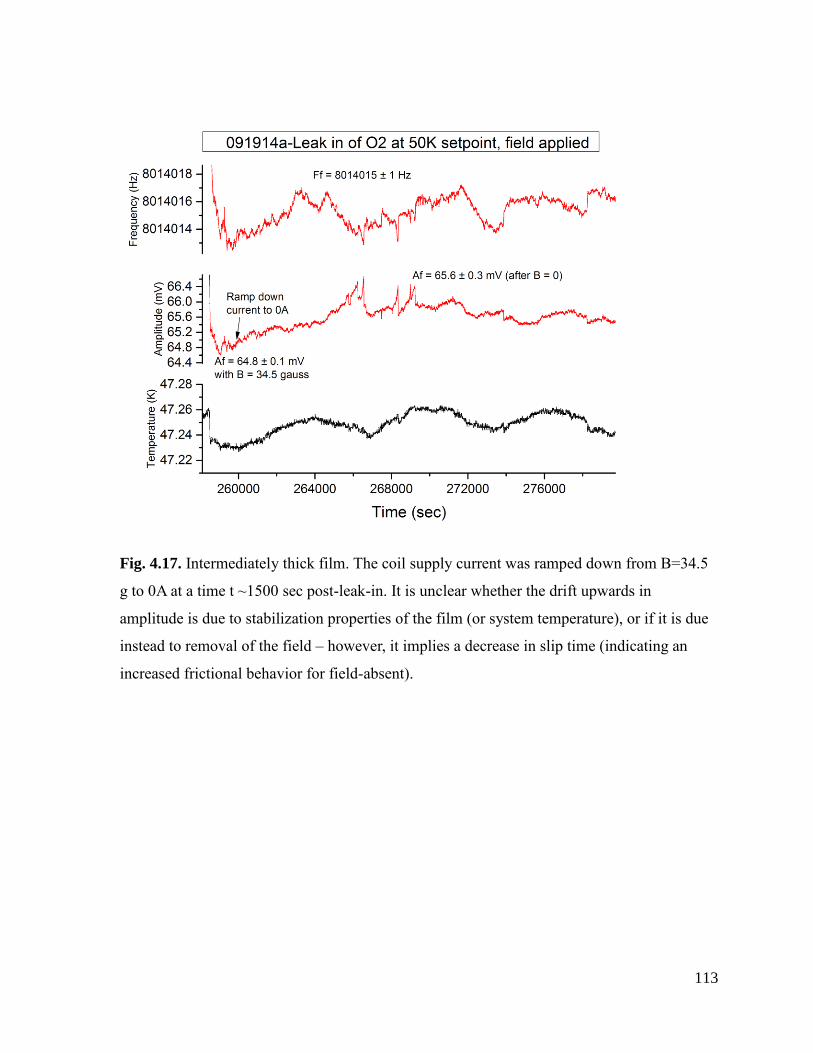
113

Fig. 4.17. Intermediately thick film. The coil supply current was ramped down from B=34.5

g to 0A at a time t ~1500 sec post-leak-in. It is unclear whether the drift upwards in

amplitude is due to stabilization properties of the film (or system temperature), or if it is due

instead to removal of the field – however, it implies a decrease in slip time (indicating an

increased frictional behavior for field-absent).

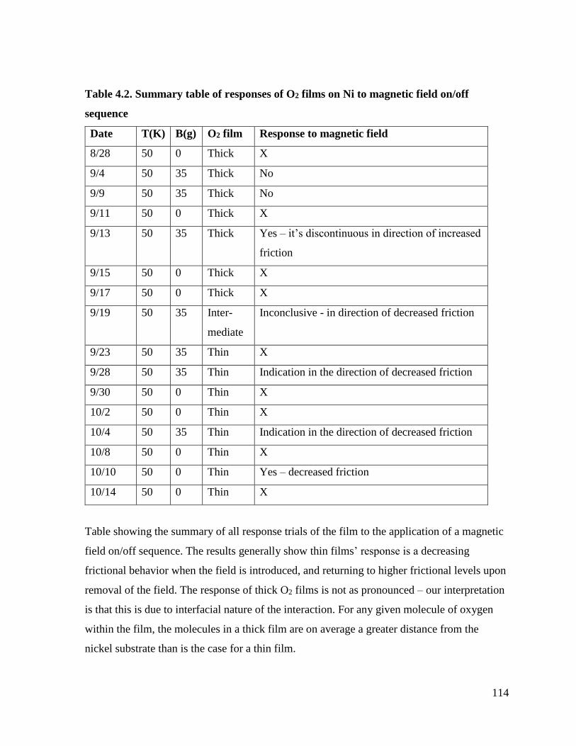
114

Table 4.2. Summary table of responses of O2 films on Ni to magnetic field on/off

sequence

Date T(K) B(g) O2 film Response to magnetic field

8/28 50 0 Thick X

9/4 50 35 Thick No

9/9 50 35 Thick No

9/11 50 0 Thick X

9/13 50 35 Thick Yes – it’s discontinuous in direction of increased

friction

9/15 50 0 Thick X

9/17 50 0 Thick X

9/19 50 35 Inter-

mediate

Inconclusive - in direction of decreased friction

9/23 50 35 Thin X

9/28 50 35 Thin Indication in the direction of decreased friction

9/30 50 0 Thin X

10/2 50 0 Thin X

10/4 50 35 Thin Indication in the direction of decreased friction

10/8 50 0 Thin X

10/10 50 0 Thin Yes – decreased friction

10/14 50 0 Thin X

Table showing the summary of all response trials of the film to the application of a magnetic

field on/off sequence. The results generally show thin films’ response is a decreasing

frictional behavior when the field is introduced, and returning to higher frictional levels upon

removal of the field. The response of thick O2 films is not as pronounced – our interpretation

is that this is due to interfacial nature of the interaction. For any given molecule of oxygen

within the film, the molecules in a thick film are on average a greater distance from the

nickel substrate than is the case for a thin film.

115

4.4 Candidate mechanisms of dissipation from O2/Ni observations

The previous sections of results of our experiments growing O2 thin films on Ni have

shown reduced friction in a field. Here we examine ways by which an applied field would

affect the state of the molecules, and thus their frictional coupling to the substrate. There are

several channels open to the system and therefore to discussion: reorientation of either the

magnetic moment (manifesting as spin friction) or the molecule’s axis (magnetostriction),

and effective viscosity change in a field (magnetorheology). To find out which of these are at

play, we will tune the system parameters of temperature, substrate composition, and

adsorbate composition. First we must understand our system - we look in the next section at

the phase diagram of 2D oxygen.

4.4.1 Structural and magnetic properties of the film-substrate systems

Oxygen is a diatomic molecule with interatomic spacing 1.21 Å and ellipsoidal shape

extending to 3.2 Å in width and 4.2 Å in length [1]. At atmospheric pressure, bulk O2 in

gaseous form condenses at 90.19 K. There are three separate bulk phases of solid oxygen:

monoclinic, orientationally ordered α phase stable below 23.8 K, rhombohedral β quasi-

orientationally ordered phase stable to 43.8 K, and cubic, orientationally disordered γ phase

which melts into the liquid, which is sterically hindered in 3D at 54.4K (Figure).

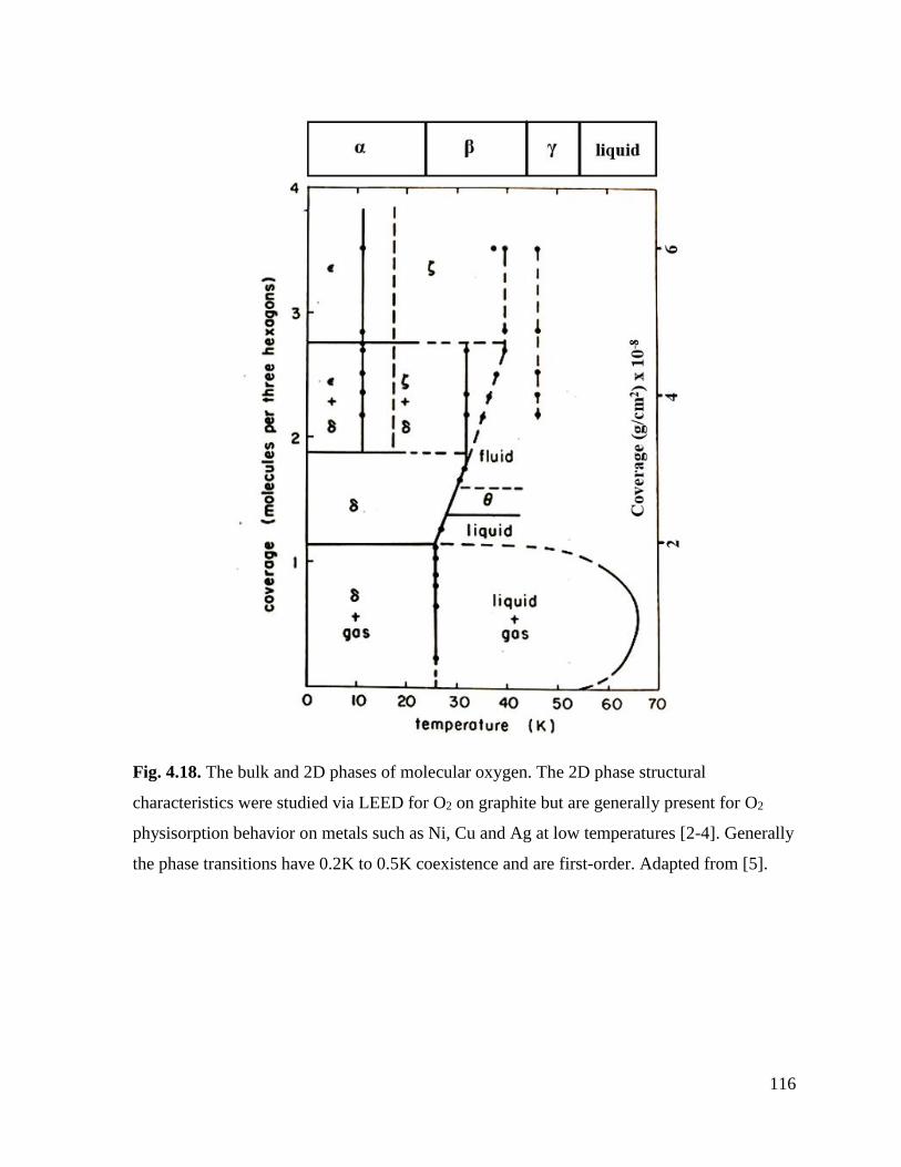
116

Fig. 4.18. The bulk and 2D phases of molecular oxygen. The 2D phase structural

characteristics were studied via LEED for O2 on graphite but are generally present for O2

physisorption behavior on metals such as Ni, Cu and Ag at low temperatures [2-4]. Generally

the phase transitions have 0.2K to 0.5K coexistence and are first-order. Adapted from [5].

117

Fig. 4.19. Schematic representation of local physical structure of various phases of 2D O2.

All phases are incommensurate on graphite. On Ni and other metals analogous δ and ζ phases

have been previously shown to occur [2-4]. (a) δ oxygen’s structure is face-centered

parallelogram, lying with its intermolecular axis plane-parallel to the substrate and is

orientationally ordered. (b) θ phase oxygen which has a triangular lattice with sterically

hindered molecular moments. (c) ζ oxygen stands upright having distorted triangular mesh

with varying ai=3.3 nearest neighbor spacing. (d) fluid phase O2, similar in structure to θ

except for epitaxially. (Adapted from [5].)

118

Fig. 4.20. Molecular orbitals (MO) of oxygen. These combined orbitals can be seen as

wavefunctions of a singular O atom which has been perturbed by the continuous introduction

of the potential and electronic orbitals of another atom O brought in adiabatically from

infinity. Thus, the orbitals are (in the LDOS framework) continuous perturbations of possible

combinatorics of both the original atom’s atomic s and p orbitals with those of the O atom

introduced. The molecule is magnetic due to the combined spin state of two unpaired

electrons in the * MO.

119

Among diatomic molecules, O2 is uniquely magnetic, owing its nonzero spin to two

uncoupled electrons in its π* molecular orbital which form an S=1 triplet – these are absent

in N2 and in general most molecules have no uncoupled electronic spin moments (Figure

4.18). The magnetic nature of molecular O2 increasingly influences the physical structure as

the temperature of oxygen is decreased – for this reason solid oxygen is referred to as a ‘spin-

controlled’ crystal and short-ranged magnetic correlations exist even in the liquid. This

molecular magnetism acts on a van-der-Waals background and enriches the phase diagram in

comparison to the simple structure of the N2 phase diagram. The α phase displays long-

ranged antiferromagnetic order, and the β shows short-ranged antiferromagnetic order. The

liquid and γ-phases are antiferromagnetic at short range, and are paramagnetic, but the

susceptibility does not closely obey Curie-Wiess temperature dependence. This has been

attributed to partial dimerization of nearest-neighbor molecules interacting

antiferromagnetically [6]. In confinement of an adsorbate to a plane, familiar 3D bulk

properties of the system such as melting temperature [7] are altered. Extensive theoretical

and experimental treatment has been conducted on 2D monolayer oxygen and multilayer

films.

Physisorbed oxygen on graphite [5,7,8] as well as both physisorbed and

chemisorption states on crystalline metals including Ni [2] have been studied in previous

literature. For a gas molecule, the electronic structure of a physisorbed species is much less

altered than the chemisorbed state. The small energy corrugation amplitude of graphite has

proven useful in previous literature to study the 2D phases of O2 [7,9]. The liquid phase, not

shown in the figure, has similar structure to fluid and has well-correlated structure. The

molecules in the liquid are rotationally disordered but have a preference to tilt towards the

surface. The δ to ζ transition is marked by the adsorbed O2 standing upright probably caused

by magnetism.

We use the 2D oxygen phase diagram here as an estimation to first-order of the film

structure and orientational behavior on our Ni and Au substrates. Upon adsorption the

molecular orientation of O2 is initially preferentially in plane, and tilts out of plane upon

increasing coverage past the first monolayer. This tilting with increased coverage has been

documented for graphite [5,7, 8] as well as for many surfaces such as Ni(111), NiO and

oxygen chemisorbed overlayers [2], Ag(110), and Cu(100) crystalline surfaces [3,4].

120

Ni is ferromagnetic in nature with magnetic moment 0.605 μB per atom. The Ni films

we have grown via e-beam evaporation and subsequent in-situ heating in presence of

hydrocarbon. AFM height trace data are included (Fig. 4.22 and 4.23). A similar process was

conducted by [11] and references therein to achieve a (possibly partially covered) graphene

surface on Ni(111), although our sample was not brought to as high of a temperature. It is

likely our sample has a range of crystallographic directions spanning (110), (100) and (111).

In low-temperature studies of oxygen adsorption onto Ni substrates, a NiO monolayer film is

formed and O2 further physisorbs upon it. The dissociated oxygen atoms are ferromagnetic

each with atomic moment 0.16 μB in contrast to many metal oxides which are

antiferromagnetic [10]. The laying-flat and standing phases are observed to occur on NiO in

analogy to δ and ζ physisorbed O2 phases elaborated on by Toney.

121

4.4.2 Magnetostriction of molecular oxygen from fluid to ζ and δ phase

Magnetostriction, a structural reorientation of elements of magnetic material in an

applied magnetic field, is a dissipation process we apply here. Humming of an electrical

transformer unit, a familiar phenomenon in everyday life, is emergent from microscopic

domain elements of magnetic core material structurally reorienting in the applied magnetic

field, and the resultant dissipation. Transformers by design incorporate materials which are

magnetically ‘soft’ as to minimize power dissipation upon re-alignment. It is known that the

liquid, θ and fluid phases of 2D adsorbed O2 have molecular alignment which is freely

rotating, but prefers to tilt in the in-plane direction. Near the boundary with the ζ phase

(molecules standing) a perpendicular magnetic field grants the molecule energy if it aligns.

The data taken on thin O2 films on Ni at 47.5 K exist in the fluid phase near this boundary

with the ζ phase, which is shown in Figure 4.16 to have phase boundaries in this region. The

δ to ζ transition in particular is considered to be driven by magnetic energies, and magnetic

energies account for 30-100K per molecule.

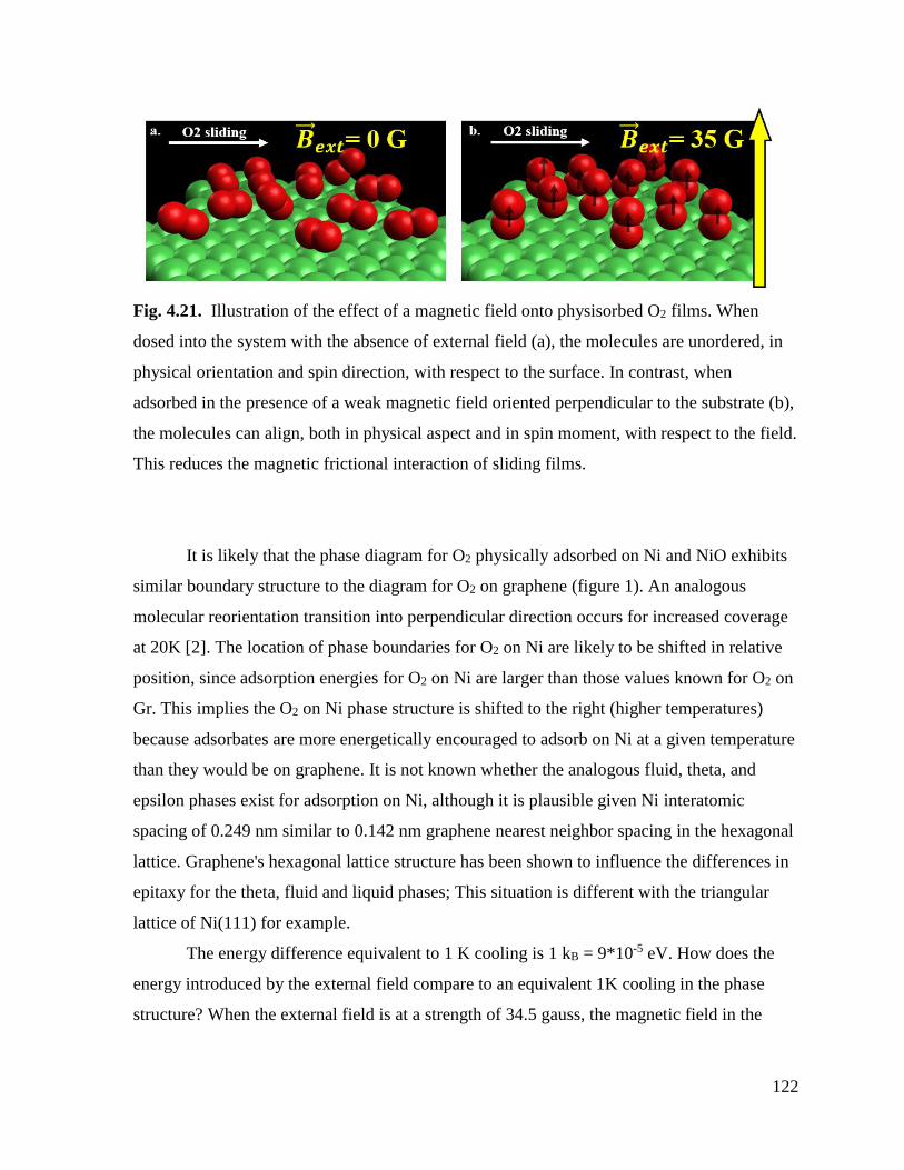
122

Fig. 4.21. Illustration of the effect of a magnetic field onto physisorbed O2 films. When

dosed into the system with the absence of external field (a), the molecules are unordered, in

physical orientation and spin direction, with respect to the surface. In contrast, when

adsorbed in the presence of a weak magnetic field oriented perpendicular to the substrate (b),

the molecules can align, both in physical aspect and in spin moment, with respect to the field.

This reduces the magnetic frictional interaction of sliding films.

It is likely that the phase diagram for O2 physically adsorbed on Ni and NiO exhibits

similar boundary structure to the diagram for O2 on graphene (figure 1). An analogous

molecular reorientation transition into perpendicular direction occurs for increased coverage

at 20K [2]. The location of phase boundaries for O2 on Ni are likely to be shifted in relative

position, since adsorption energies for O2 on Ni are larger than those values known for O2 on

Gr. This implies the O2 on Ni phase structure is shifted to the right (higher temperatures)

because adsorbates are more energetically encouraged to adsorb on Ni at a given temperature

than they would be on graphene. It is not known whether the analogous fluid, theta, and

epsilon phases exist for adsorption on Ni, although it is plausible given Ni interatomic

spacing of 0.249 nm similar to 0.142 nm graphene nearest neighbor spacing in the hexagonal

lattice. Graphene's hexagonal lattice structure has been shown to influence the differences in

epitaxy for the theta, fluid and liquid phases; This situation is different with the triangular

lattice of Ni(111) for example.

The energy difference equivalent to 1 K cooling is 1 kB = 9*10-5 eV. How does the

energy introduced by the external field compare to an equivalent 1K cooling in the phase

structure? When the external field is at a strength of 34.5 gauss, the magnetic field in the

123

vicinity of Ni is 360 gauss due to the magnetization field of Ni. The Zeeman energy

associated with an oxygen molecular spin moment orienting in field is:

𝐸𝑧 = 3.6 ∗ 10−2 ∗ 2 μ𝐵 = 4.2 ∗ 10−6 eV (4.1)

which is about 5% of the equivalent thermal energy lost by cooling 1K. In the region of the

phase diagram close to a transition, it is possible for a field to bring the system across the

transition solely due to Zeeman energy supplied by the field. Our data on O2 on Ni films take

place at 47K and are lying within 5K of the transition to ζ. This transition is known to be

broad, showing coexistence of both phases within 0.5K of the boundary.

For an oxygen molecule existing as member of a film, magnetic exchange also plays

a role in the total magnetic energy of the O2 molecule. Magnetic energies for the oxygen

intermolecular interaction are estimated to be 40 K [12] at 3.2 angstroms, with an exponential

dependence on distance, whereas average vdW adsorption energy on graphite is 1122 K

[5,9]. Because the magnetic exchange between oxygen molecules is non-negligible for the

condensed phases, behavior in an external field will be much more pronounced than just that

expected by Zeeman splitting (which is typically the valid treatment for non-interacting

moments). The bulk γ oxygen phase and bulk liquid are known to have short-ranged

antiferromagnetic order. For antiferromagnetism, the exchange constant is negative. For this

reason if the ζ phase is ordered antiferromagnetically, due to its (approximately) triangular

lattice, it is likely to be magnetically frustrated.

Thus far, we have considered the orientation direction of the molecular magnetic

moment to be rigidly coupled to the interatomic axis direction. We consider also the situation

of the field application causing the molecular magnetic moments to align while the physical

structure of the molecule stays un-aligned (which is discussed further in the magnetorheology

section below). The spin-spin energy of an oxygen molecule is 0.13 meV in preference for

the interatomic axis as compared to lying in the plane perpendicular to the molecular axis

[13]. Since this energetic preference is larger by a factor of 30 than the Bext – dipole field

energy, we can consider the spin moment of O2 to be rigidly attached to its axis, meaning a

change in the magnetic moment direction causes a concomitant change in the physical

orientation of the molecule. In some low temperature phases of adsorbed oxygen, the

magnetic moments point in a direction other than the molecular axis, in these situations a

vdW-exchange competition takes place.

124

Magnetic thin films exhibit magnetization reorientation in removal of field due to

shape anisotropy. If this phenomenon is present in our films, it implies that the Bext absent

condition causes the remanent field in the nickel film to reorient in an in-plane direction,

perhaps causing the adsorbate molecules follow suit and lay flat, further encouraging them to

mimic the δ phase. This expectation underlies our interpretation of the incremental warmup

data of O2 on Ni. The increased frictional levels observed in our data upon lowering of the

system temperature from 47K through 30K for film coverages in the ρ = 50 ng/cm2 region

implies the films have undergone a transition from fluid to δ + ζ phase, here preferring the δ

phase due to the in-plane remanent field M = 60 g expected to be present near the nickel.

So far in this section we have discussed the way in which a field reorients a

molecule’s axis. To explain the impact of the physical orientation of the molecule upon its

frictional interaction with the substrate, we turn to an energy corrugation amplitude

framework. A given substrate has lateral modulations in the van der Walls energy of an

adsorbate molecule attached to the surface. The slip time of an adsorbed layer due to phonon

friction depends on the adsorbate-substrate corrugation amplitude [14,15]:

𝜏 ∝ 𝑓−2 (4.2)

Where τ is slip time and f is corrugation amplitude. In order to account for a factor of 1.8

increase in slip time when field is applied:

𝜏𝐵

𝜏0=

𝑓02

𝑓𝐵2 = 1.8

(4.3)

Where τB is slip time in field, τ0 is slip time in absence of field, fB is amplitude in field and f0

is amplitude in absence of field. The van der Waals potential between two particles follows a

6-12 form, which is dominated by the 1/r6 dependence beyond the adsorption distance, which

is the realm we are considering:

𝑈 = 𝐸𝐿𝐽 ∝

1

𝑟6

(4.4)

Integrating this interaction over the surface [16] yields an interaction law:

𝑈(𝑟) ∝

1

𝑟3

(4.5)

125

Which implies that for differences in adsorbate energies:

𝑓 = |𝑈𝑎𝑡𝑜𝑚 − 𝑈𝑠𝑖𝑡𝑒| ⇒ 𝑓 ∝

1

𝑟3

(4.6)

Plugging this into the above dependence, we have:

𝜏𝐵

𝜏0=

𝑟𝐵6

𝑟06

(4.7)

Our equilibrium adsorption distance for O2 on gr, 3.2 Å [5] gives us an effective field

adsorption distance:

𝑟𝐵 = √1.8 ∗ 3.266= 3.5 Å (4.8)

This implies that when the molecule stands upright, its effective adsorption amplitude is

lessened by an amount corresponding to a displacement by:

𝛿𝑟 = 𝑟𝐵 − 𝑟0 = 3.5 − 3.2 Å = 0.3 Å (4.9)

If we consider the ellipsoidal shape of the O2, the short axis radius is 1.6 Å and the long axis

radius is 2.1 Å, and the difference between these is 0.5 Å. Simply by accounting for shape

anisotropy we are within the bounds for an explanation of the frictional behavior in a field.

A freely rotating O2 molecule on graphene has energy difference 1149K – 1112K =

37K = 3.2 meV, which we refer to as corrugation amplitude, between site and atom

adsorption positions. For O2 on Ni or NiO the corrugation energy amplitude is assumed to be

larger, because graphene is known to be relatively ‘flat’ in terms of van der Waals adsorption

as compared to most substrates. The above treatment is in fact independent of corrugation

amplitude value. The shift in effective adsorption distance is solely dependent on original

adsorption distance, which for O2 on NiO is expected to be smaller than for O2 on graphene.

Other subtleties exist; the oxygen molecule has a polarizability anisotropy κ which alters the

van der walls binding dependent on direction. As well, washboard frequency is changed [17].

For the purposes of phononic friction, the polarizability is the same for molecular orientation

parallel or anti-parallel, since for both of these alignments the molecule is standing. So this

treatment works for antiferromagnetic state as if it were ferromagnetic.

This mechanism of magnetostriction explains the decrease in friction for the thin O2

film on Ni in applied field, and predicts a frictional increase upon transition from the fluid to

the delta phase, for which the films are flat, and therefore closer to the surface.

126

4.4.3 Spin Friction

For atomic sliding on an atomically smooth surface, typically van der Waals forces

are considered to dominate the behavior. It has been demonstrated by Coffey and Krim that

the dissipation rate is directly proportional to the square of the substrate’s energy corrugation

amplitude [15]. For sliding of a magnetized atom relative to a magnetic material, it has been

further demonstrated that the spin lattice can be superimposed on the crystal lattice, and this

consideration alters the energy corrugation, and thus the friction [18]. So this framework

adds the magnetic exchange energy consideration to the existing van der Waals picture. The

spin lattice can be either ferromagnetic (FM) or anti-ferromagnetic (AFM).

Exchange force is a force of repulsion for identical fermions. It is not really a force

but a purely geometrical consequence of the symmetrization requirement:

Ψ(𝒓𝟏, 𝒓𝟐) = ±Ψ(𝒓𝟐, 𝒓𝟏) (4.10)

Where Ψ is the total wavefunction of the two particles and + is used for identical bosons and

– is used for identical fermions (which electrons are). The total wavefunction of a given

electron can be decomposed into spin and spatial components:

Ψ(𝒓) = 𝝍(𝒓)χ(𝒓) (4.11)

When the wavefunctions of the two electrons overlap, the whole wavefunction must be

antisymmetric with respect to exchange of the two. This exchange energy for O2-O2 is 40K

and depends on intermolecular distance with an exponential decay.

If the field is not applied and the molecular spin orientations are unrestricted, this is

the magnetic analogy to a physical liquid state. When the field is applied and the moments

lock into alignment (or anti-alignment for the case of antiferromagnetic films), this represents

a solid magnetic state. Thus the entropy of the system cannot flow into the spin lattice and

this dissipation channel is suppressed.

In the literature review of chapter 2 we discussed computational results [18]

highlighting the frictional decrease when a film was magnetized as compared to the

unmagnetized state. The authors attributed this decreased energy corrugation to repulsive

exchange interactions across the interface between individual magnetized substrate atoms

and magnetized adsorbates. This picture is consistent with our results above of field

decreasing friction of O2 on Ni, and does not require the molecules to physically re-align in

the field (such as for magnetostriction), merely for their magnetic moments to be locked in

127

alignment. This spin friction explanation predicts for our system a decrease in friction upon

cooling from liquid into the δ phase, as the paramagnetic susceptibility shows an increase

down to 30K [5]. The magnetostriction picture painted above predicts the opposite. We use

this distinction between the two explanations to guide us into the next phase of data taking as

a means to find out which dissipation channel is dominant in our system. In the next phase,

we entered the δ phase through cooling a film grown at 47K through incremental setpoints to

27K. However, we must move first to the last of our candidate mechanisms of

magnetorheology.

4.4.4 Magnetorheology

Magnetorheological (MR) fluids are colloidal suspensions of micron-scale

ferromagnetic Fe, Ni, or Co particles in a medium - typically silicone oil, synthetic

hydrocarbon or esters, kerosene, toluene, etc, or even water-based. Their structure and

viscosity reversibly change upon introduction of a magnetic field, which magnetizes the

particles and aggregates them into chains. Some of the many applications of MR fluids are in

digital data storage, resonance imaging [19]; magnetic fluid linear pumps; audio speakers,

smart materials, automobile clutch and braking systems, helicopter rotors [20] and haptic

feedback interfaces [21].

Parameters that can be tuned to suit the requirements of the system are field

orientation with respect to flow direction, chemical makeup and shape of particles including

rod-like and spherical, thixotropic agent presence and type, carrier fluid characteristics, and

steric coating characteristics. Recently the tribological aspects of thin-film MR fluids have

been elucidated, in one case measuring a fourfold increase in friction with applied field

present.QCM studies of magnetorheological fluids have been studied recently, showing

damping to be proportional to applied field [22]

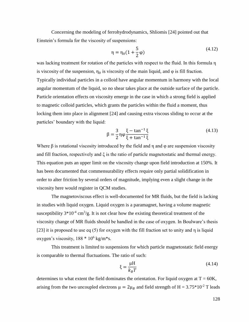
128

Concerning the modeling of ferrohydrodynamics, Shliomis [24] pointed out that

Einstein’s formula for the viscosity of suspensions:

η = η0(1 +

5

2φ)

(4.12)

was lacking treatment for rotation of the particles with respect to the fluid. In this formula η

is viscosity of the suspension, η0 is viscosity of the main liquid, and φ is fill fraction.

Typically individual particles in a colloid have angular momentum in harmony with the local

angular momentum of the liquid, so no shear takes place at the outside surface of the particle.

Particle orientation effects on viscosity emerge in the case in which a strong field is applied

to magnetic colloid particles, which grants the particles within the fluid a moment, thus

locking them into place in alignment [24] and causing extra viscous sliding to occur at the

particles’ boundary with the liquid:

β =

3

2ηφ

ξ − tan−1 ξ

ξ + tan−1 ξ

(4.13)

Where β is rotational viscosity introduced by the field and η and φ are suspension viscosity

and fill fraction, respectively and ξ is the ratio of particle magnetostatic and thermal energy.

This equation puts an upper limit on the viscosity change upon field introduction at 150%. It

has been documented that commensurability effects require only partial solidification in

order to alter friction by several orders of magnitude, implying even a slight change in the

viscosity here would register in QCM studies.

The magnetoviscous effect is well-documented for MR fluids, but the field is lacking

in studies with liquid oxygen. Liquid oxygen is a paramagnet, having a volume magnetic

susceptibility 3*10-4 cm3/g. It is not clear how the existing theoretical treatment of the

viscosity change of MR fluids should be handled in the case of oxygen. In Boulware’s thesis

[23] it is proposed to use eq (5) for oxygen with the fill fraction set to unity and η is liquid

oxygen’s viscosity, 188 * 106 kg/m*s.

This treatment is limited to suspensions for which particle magnetostatic field energy

is comparable to thermal fluctuations. The ratio of such:

ξ =

μH

𝑘𝐵𝑇

(4.14)

determines to what extent the field dominates the orientation. For liquid oxygen at T = 60K,

arising from the two uncoupled electrons μ = 2μ𝐵 and field strength of H = 3.75*10-2 T leads

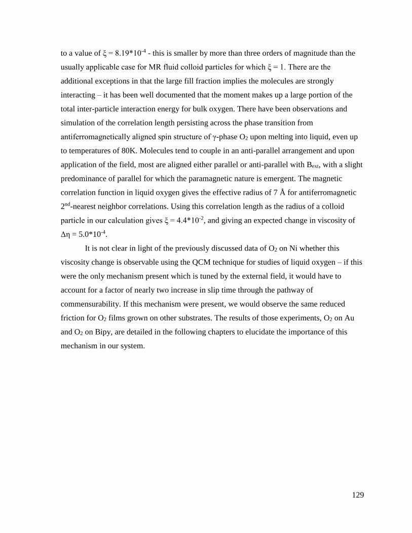
129

to a value of ξ = 8.19*10-4 - this is smaller by more than three orders of magnitude than the

usually applicable case for MR fluid colloid particles for which ξ = 1. There are the

additional exceptions in that the large fill fraction implies the molecules are strongly

interacting – it has been well documented that the moment makes up a large portion of the

total inter-particle interaction energy for bulk oxygen. There have been observations and

simulation of the correlation length persisting across the phase transition from

antiferromagnetically aligned spin structure of γ-phase O2 upon melting into liquid, even up

to temperatures of 80K. Molecules tend to couple in an anti-parallel arrangement and upon

application of the field, most are aligned either parallel or anti-parallel with Bext, with a slight

predominance of parallel for which the paramagnetic nature is emergent. The magnetic

correlation function in liquid oxygen gives the effective radius of 7 Å for antiferromagnetic

2nd-nearest neighbor correlations. Using this correlation length as the radius of a colloid

particle in our calculation gives ξ = 4.4*10-2, and giving an expected change in viscosity of

Δη = 5.0*10-4.

It is not clear in light of the previously discussed data of O2 on Ni whether this

viscosity change is observable using the QCM technique for studies of liquid oxygen – if this

were the only mechanism present which is tuned by the external field, it would have to

account for a factor of nearly two increase in slip time through the pathway of

commensurability. If this mechanism were present, we would observe the same reduced

friction for O2 films grown on other substrates. The results of those experiments, O2 on Au

and O2 on Bipy, are detailed in the following chapters to elucidate the importance of this

mechanism in our system.

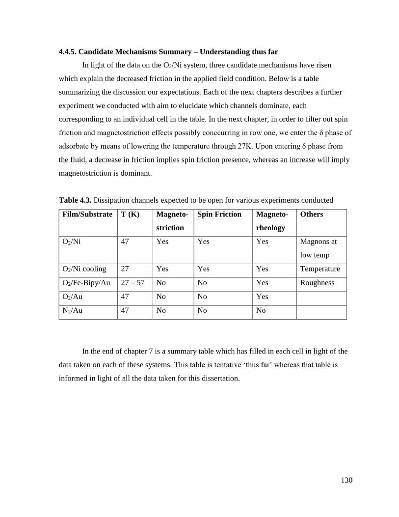
130

4.4.5. Candidate Mechanisms Summary – Understanding thus far

In light of the data on the O2/Ni system, three candidate mechanisms have risen

which explain the decreased friction in the applied field condition. Below is a table

summarizing the discussion our expectations. Each of the next chapters describes a further

experiment we conducted with aim to elucidate which channels dominate, each

corresponding to an individual cell in the table. In the next chapter, in order to filter out spin

friction and magnetostriction effects possibly conccurring in row one, we enter the δ phase of

adsorbate by means of lowering the temperature through 27K. Upon entering δ phase from

the fluid, a decrease in friction implies spin friction presence, whereas an increase will imply

magnetostriction is dominant.

Table 4.3. Dissipation channels expected to be open for various experiments conducted

Film/Substrate T (K) Magneto-

striction

Spin Friction Magneto-

rheology

Others

O2/Ni 47 Yes Yes Yes Magnons at

low temp

O2/Ni cooling 27 Yes Yes Yes Temperature

O2/Fe-Bipy/Au 27 – 57 No No Yes Roughness

O2/Au 47 No No Yes

N2/Au 47 No No No

In the end of chapter 7 is a summary table which has filled in each cell in light of the

data taken on each of these systems. This table is tentative ‘thus far’ whereas that table is

informed in light of all the data taken for this dissertation.

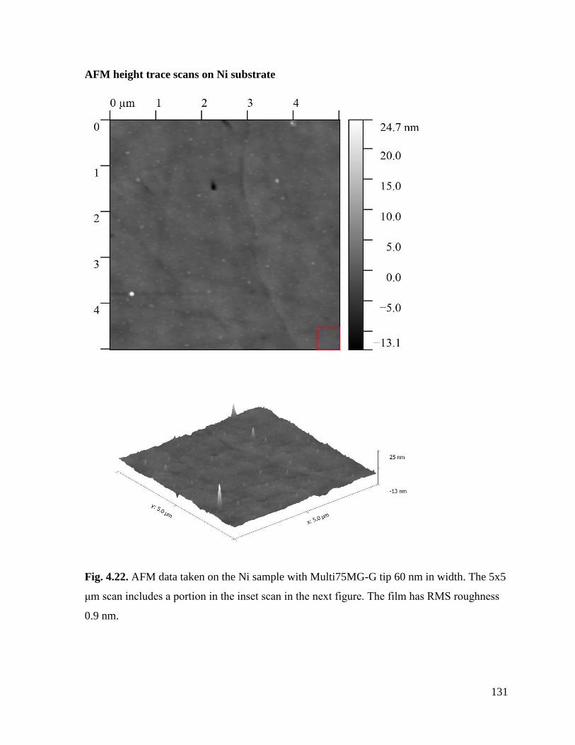
131

AFM height trace scans on Ni substrate

Fig. 4.22. AFM data taken on the Ni sample with Multi75MG-G tip 60 nm in width. The 5x5

μm scan includes a portion in the inset scan in the next figure. The film has RMS roughness

0.9 nm.

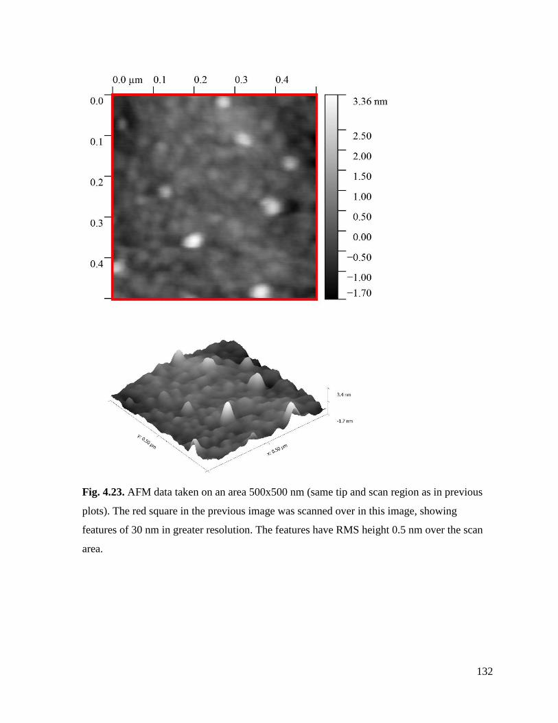
132

Fig. 4.23. AFM data taken on an area 500x500 nm (same tip and scan region as in previous

plots). The red square in the previous image was scanned over in this image, showing

features of 30 nm in greater resolution. The features have RMS height 0.5 nm over the scan

area.

133

REFERENCES CHAPTER 4

[1] R.F. Bader,W.H. Henneker, P.E. Cade, J. Chem. Phys. 46 (1967) 3341.

[2] Aoki, M., Taoka, H., Kamada, T., & Masuda, S. (2001). Local electronic states of

oxygen on Ni(111) surface studied by metastable atom electron spectroscopy. Journal of

Electron Spectroscopy and Related Phenomena, 114-116 (2001) 507-512.

[3] Kazama, Y., Matsumoto, M., Sugimoto, T., Okano, T., & Fukutani, K. (2011). Low-

temperature surface phase and phase transition of physisorbed oxygen on the Ag(111)

surface. Physical Review B - Condensed Matter and Materials Physics, 84(April), 4–6.

http://doi.org/10.1103/PhysRevB.84.064128

[4] Kurahashi, M., Sun, X., & Yamauchi, Y. (2012). Magnetic properties of O2 adsorbed on

Cu(100): A spin-polarized metastable He beam study. Physical Review B - Condensed

Matter and Materials Physics, 86, 1–2. http://doi.org/10.1103/PhysRevB.86.245421

[5] Toney, M.F. (1983). Low-Energy Electron Diffraction Study of Molecular Oxygen

Physisorbed on Graphite. (Doctoral dissertation).

[6] Oda, T., & Pasquarello, A. (2004). Noncollinear magnetism in liquid oxygen: A first-

principles molecular dynamics study. Physical Review B 70, 134402.

[7] Chiarello, R., Coulomb, J.P., Krim, J., &Wang, L. (1988). Surface melting of multilayer

oxygen films on graphite studied by neutron diffraction. Physical Review B 38-13.

[8] Marx, R., & Christoffer, B. (1985). Magnetocaloric effects of 2D adsorbed O2. Journal of

Physics C: Solid State Physics, 18, 2849–2858. http://doi.org/10.1088/0022-3719/18/14/016

[9] Toney, M.F., & Fain, S.C. Jr. (1987). Low-energy electron diffraction study of molecular

oxygen physisorbed on graphite. Physical Review B 36-2.

[10] 33. Yamagishi, S., Jenkins, S. J., & King, D. a. (2003). First principles studies of

chemisorbed O on Ni{1 1 1}. Surface Science, 543(April), 12–18.

http://doi.org/10.1016/j.susc.2003.08.002

[11] Winder, S.M. (2003). Quartz Crystal Microbalance Measurements of Sliding Friction of

Inert Gas Films on Lead, Copper, Nickel and Graphene Surfaces. (Doctoral dissertation).

[12] Freimann, Y.A., & Jodl, H.J. (2004). Solid Oxygen. Physics Reports 401 1-228.

[13] Herzberg, G. (1939). Molecular Spectra and Molecular Structure I. Diatomic

Molecules. New York: Prentice Hall, Inc.

[14] Cieplak, M., Smith, E. D., & Robbins, M. (1994). Molecular Origins of Friction : The

Force on Adsorbed Layers, 265(5176), 1209–1212.

134

[15] Coffey, T., & Krim, J. (2005). Impact of substrate corrugation on the sliding friction

levels of adsorbed films. Physical Review Letters, 95(August), 1–4.

http://doi.org/10.1103/PhysRevLett.95.076101

[16] Krim, J. (1984). Wetting Behavior of Simple Molecular Gases Physically Adsorbed on

Au(111). (Doctoral dissertation).

[17] Daly, C., & Krim, J. (1996). Friction and dampling of Xe/Ag(111). Surface Science 49-

54.

[18] 7. Cai, X., Wang, J., Li, J., Sun, Q., & Jia, Y. (2016). Spin friction between Co

monolayer and Mn/W(110) surface: Ab Initio investigations. Tribology International, 95,

419–425. http://doi.org/10.1016/j.triboint.2015.11.037

[19] Boulware, J. C., Ban, H., Jensen, S., & Wassom, S. (2010). Experimental studies of the

pressures generated by a liquid oxygen slug in a magnetic field. Journal of Magnetism and

Magnetic Materials, 322(13), 1752–1757. http://doi.org/10.1016/j.jmmm.2009.12.022

[20] Bombard, A. J. F., & De Vicente, J. (2012). Thin-film rheology and tribology of

magnetorheological fluids in isoviscous-EHL contacts. Tribology Letters, 47(6), 149–162.

http://doi.org/10.1007/s11249-012-9971-2

[21] Rizzo, R., Sgambelluri, N., Scilingo, E. P., Raugi, M., & Bicchi, a. (2007).

Electromagnetic modeling and design of haptic interface prototypes based on

magnetorheological fluids. IEEE Transactions on Magnetics, 43(9), 3586–3599.

http://doi.org/10.1109/TMAG.2007.901351

[22] Rodriguez-López, J., Castro, P., de Vicente, J., Johannsmann, D., Elvira, L., Morillas, J.,

& Montero de Espinosa, F. (2015). Colloidal Stability and Magnetic Field-Induced Ordering

of Magnetorheological Fluids Studied with a Quartz Crystal Microbalance. Sensors, 15,

30443–30456. http://doi.org/10.3390/s151229808

[23] Boulware, J. C. (2010). Experiment and Simulation on the Dynamics of a Slug of Liquid

Oxygen Displaced by a Pulsed Magnetic Field. (Doctoral dissertation). Retrieved from:

http://digitalcommons.usu.edu/etd.

[24] Shliomis, M. I. (1974). Magnetic fluids. Soviet Physics Usp, 17.

135

CHAPTER 5 - RESULTS OF EXPERIMENTS INCREMENTALLY COOLING O2

FILMS ON NI

In the previous chapter was described a dependence on field at 47K. In this next set of

data runs, we brought O2 monolayer films into the δ phase. At 47K through the transition

from fluid to δ phase in absence of field to ascertain if friction depends on orientation. The

frictional dependence which we observe on temperature, and thus phase, will elucidate which

dissipation mechanism is dominant in our O2/Ni data on which we previously elaborated. An

observed increase in friction for this data upon cooling into δ phase shows that

magnetostriction channels are open in our system. Our interpretation is that spin friction

effects are not as important, for they would predict a decrease in friction upon reduction of

temperature. For a discussion of the relevant mechanisms, see previous chapter.

O2 thin films were grown on Ni at 47K in absence of field in a similar manner to the

chapter 4 data. The exception is that prior to the film growth, the sample was brought in

UHV through four incremental temperatures 26K, 34K, 42K and 47K – once at each setpoint

for each vacuum and film condition. The amplitude and frequency traces were allowed to

stabilize at equilibrium values at each setpoint temperature, and the film absent data were

subtracted from the film present to gain insight to the system’s friction temperature

dependence.

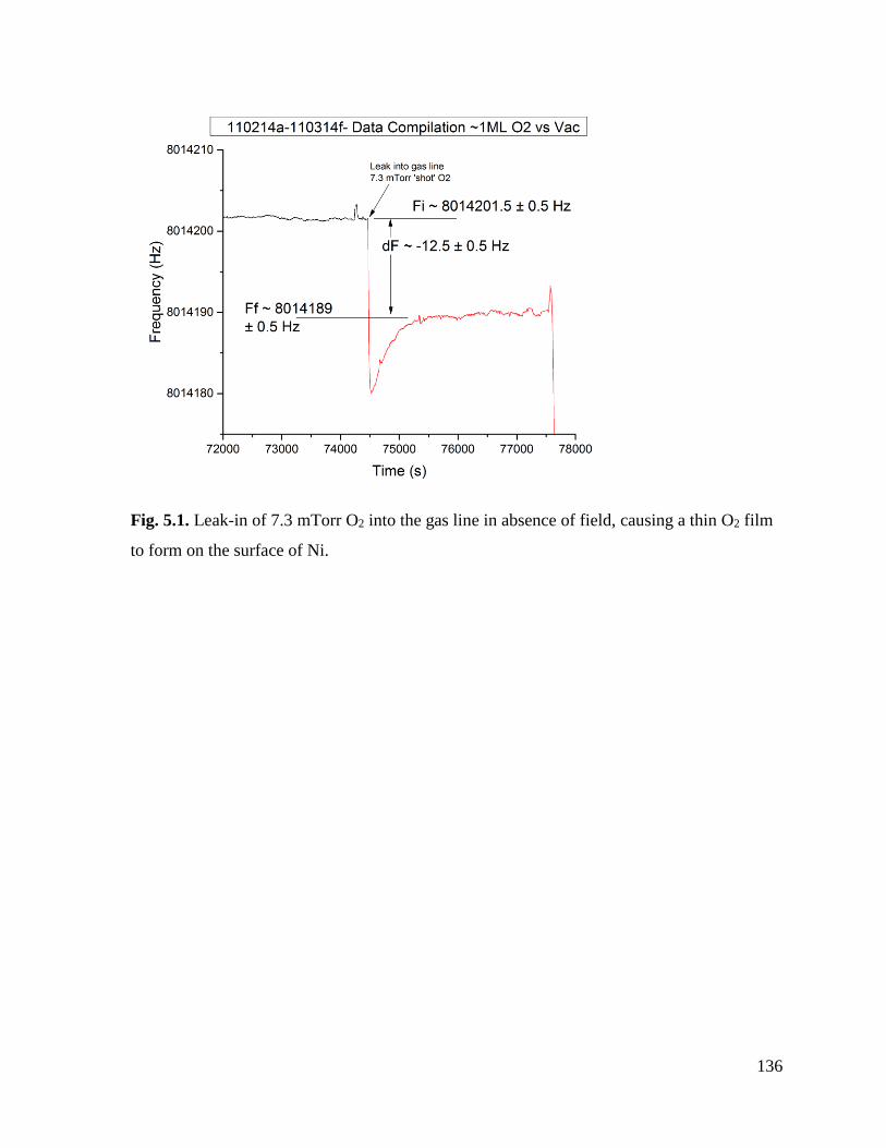
136

Fig. 5.1. Leak-in of 7.3 mTorr O2 into the gas line in absence of field, causing a thin O2 film

to form on the surface of Ni.

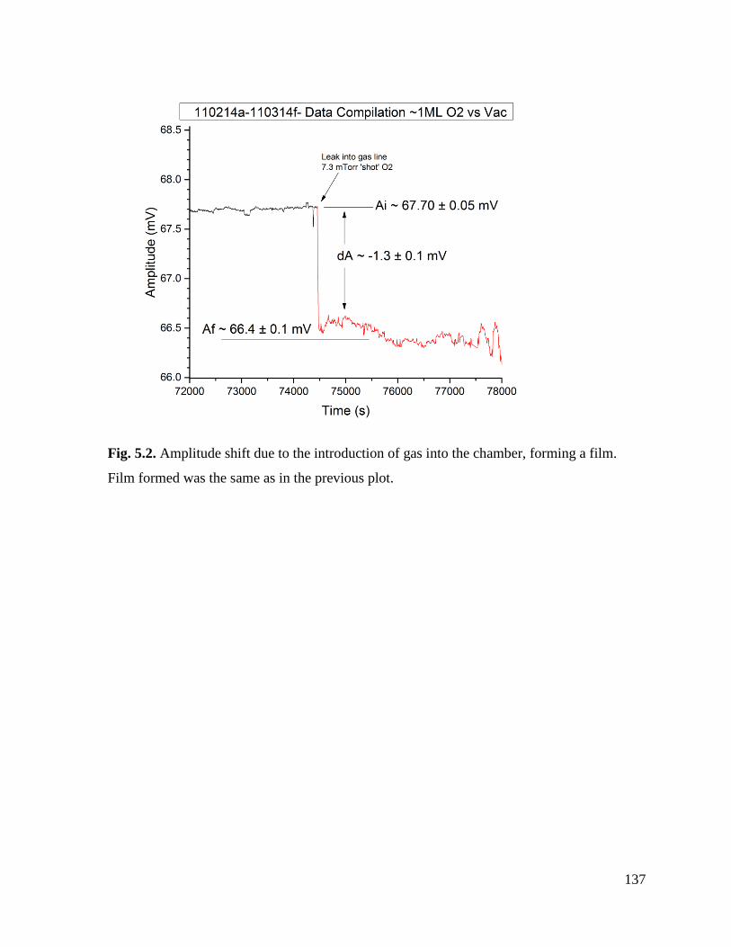
137

Fig. 5.2. Amplitude shift due to the introduction of gas into the chamber, forming a film.

Film formed was the same as in the previous plot.

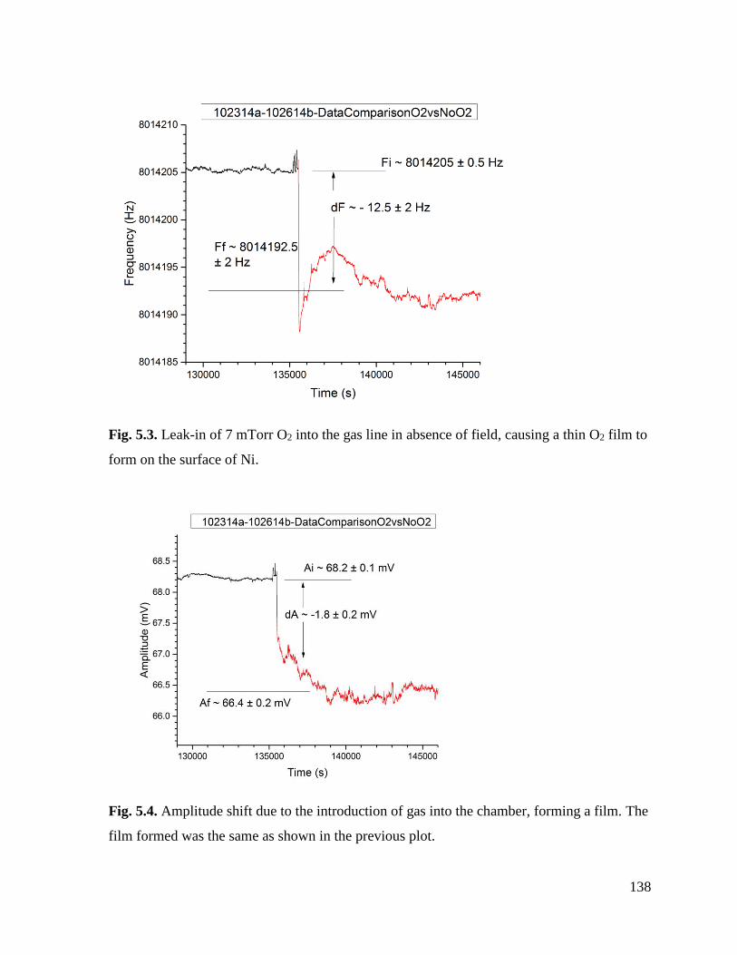
138

Fig. 5.3. Leak-in of 7 mTorr O2 into the gas line in absence of field, causing a thin O2 film to

form on the surface of Ni.

Fig. 5.4. Amplitude shift due to the introduction of gas into the chamber, forming a film. The

film formed was the same as shown in the previous plot.

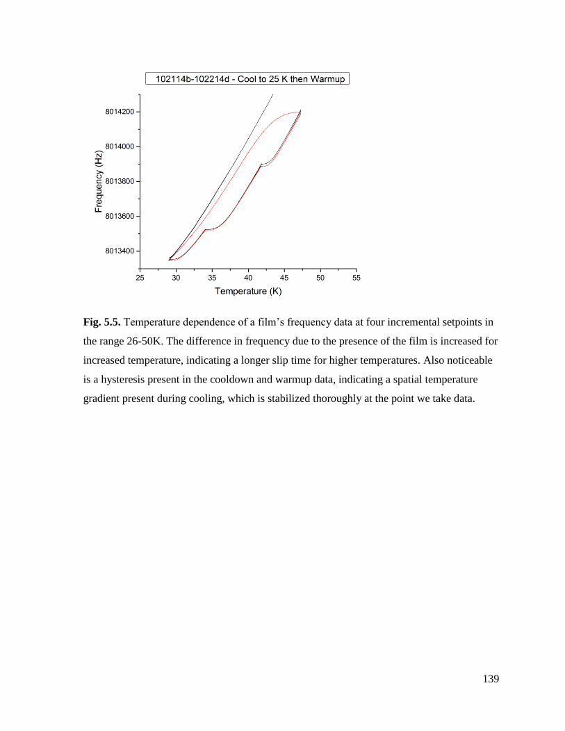
139

Fig. 5.5. Temperature dependence of a film’s frequency data at four incremental setpoints in

the range 26-50K. The difference in frequency due to the presence of the film is increased for

increased temperature, indicating a longer slip time for higher temperatures. Also noticeable

is a hysteresis present in the cooldown and warmup data, indicating a spatial temperature

gradient present during cooling, which is stabilized thoroughly at the point we take data.

140

Fig. 5.6. Temperature dependence of a film’s amplitude data at four setpoints in the range

26-50K. The difference in amplitude due to the presence of the film is increased for increased

temperature, indicating a longer slip time for higher temperatures. The hysteresis is present in

the cooldown and warmup data, indicating the spatial temperature gradient present during

cooling. This amplitude data corresponds to the film grown in the previous plot’s frequency

data. At each of the four setpoints we calculate the slip time by subtracting out the frequency

and amplitude values for the film present case from their respective values in the film absent

case.

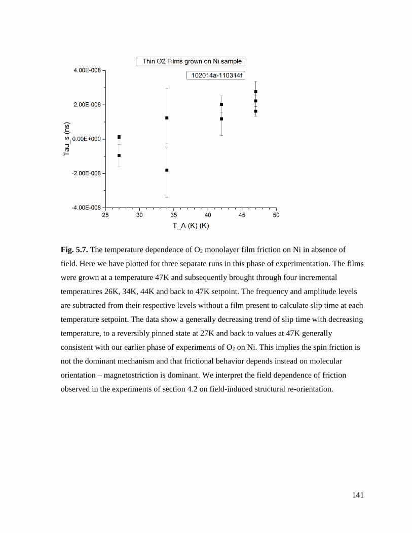
141

Fig. 5.7. The temperature dependence of O2 monolayer film friction on Ni in absence of

field. Here we have plotted for three separate runs in this phase of experimentation. The films

were grown at a temperature 47K and subsequently brought through four incremental

temperatures 26K, 34K, 44K and back to 47K setpoint. The frequency and amplitude levels

are subtracted from their respective levels without a film present to calculate slip time at each

temperature setpoint. The data show a generally decreasing trend of slip time with decreasing

temperature, to a reversibly pinned state at 27K and back to values at 47K generally

consistent with our earlier phase of experiments of O2 on Ni. This implies the spin friction is

not the dominant mechanism and that frictional behavior depends instead on molecular

orientation – magnetostriction is dominant. We interpret the field dependence of friction

observed in the experiments of section 4.2 on field-induced structural re-orientation.

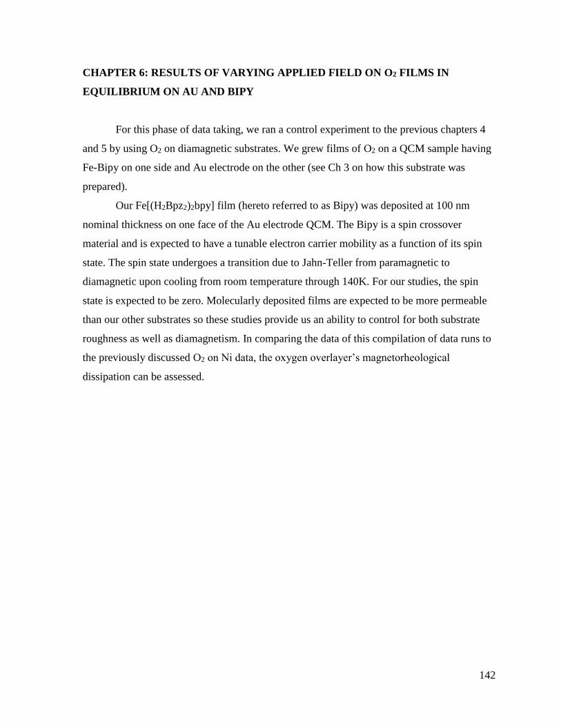
142

CHAPTER 6: RESULTS OF VARYING APPLIED FIELD ON O2 FILMS IN

EQUILIBRIUM ON AU AND BIPY

For this phase of data taking, we ran a control experiment to the previous chapters 4

and 5 by using O2 on diamagnetic substrates. We grew films of O2 on a QCM sample having

Fe-Bipy on one side and Au electrode on the other (see Ch 3 on how this substrate was

prepared).

Our Fe[(H2Bpz2)2bpy] film (hereto referred to as Bipy) was deposited at 100 nm

nominal thickness on one face of the Au electrode QCM. The Bipy is a spin crossover

material and is expected to have a tunable electron carrier mobility as a function of its spin

state. The spin state undergoes a transition due to Jahn-Teller from paramagnetic to

diamagnetic upon cooling from room temperature through 140K. For our studies, the spin

state is expected to be zero. Molecularly deposited films are expected to be more permeable

than our other substrates so these studies provide us an ability to control for both substrate

roughness as well as diamagnetism. In comparing the data of this compilation of data runs to

the previously discussed O2 on Ni data, the oxygen overlayer’s magnetorheological

dissipation can be assessed.

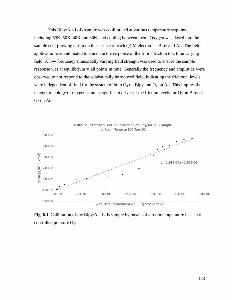
143

This Bipy/Au-1s-B sample was equilibrated at various temperature setpoints

including 60K, 50K, 40K and 30K, and cooling between them. Oxygen was dosed into the

sample cell, growing a film on the surface of each QCM electrode - Bipy and Au. The field

application was automated to elucidate the response of the film’s friction to a time varying

field. A low frequency sinusoidally varying field strength was used to ensure the sample

response was at equilibrium at all points in time. Generally the frequency and amplitude were

observed to not respond to the adiabatically introduced field, indicating the frictional levels

were independent of field for the system of both O2 on Bipy and O2 on Au. This implies the

magnetorheology of oxygen is not a significant driver of the friction levels for O2 on Bipy or

O2 on Au.

Fig. 6.1. Calibration of the Bipy/Au-1s-B sample by means of a room temperature leak-in of

controlled pressure O2.

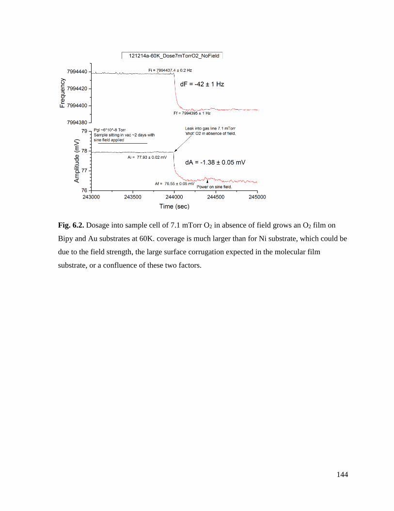
144

Fig. 6.2. Dosage into sample cell of 7.1 mTorr O2 in absence of field grows an O2 film on

Bipy and Au substrates at 60K. coverage is much larger than for Ni substrate, which could be

due to the field strength, the large surface corrugation expected in the molecular film

substrate, or a confluence of these two factors.

145

Fig. 6.3. Magnetic field with sinusoidal time dependent field strength applied to an O2 thin

film on Bipy and Au at T_s = 60K. No distinct change happens in the frictional state of the

film due to the introduction of the field.

146

Fig. 6.4. Frequency vs absolute value of applied field of an O2 thin film at T_s = 60K.

Frequency data is independent of abs(field) for this time interval, to within 0.3 Hz

uncertainty.

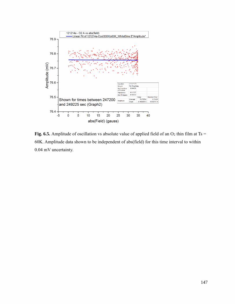
147

Fig. 6.5. Amplitude of oscillation vs absolute value of applied field of an O2 thin film at Ts =

60K. Amplitude data shown to be independent of abs(field) for this time interval to within

0.04 mV uncertainty.

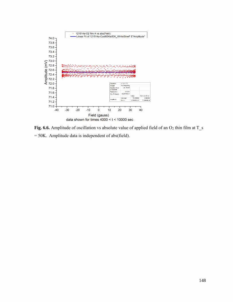
148

Fig. 6.6. Amplitude of oscillation vs absolute value of applied field of an O2 thin film at T_s

= 50K. Amplitude data is independent of abs(field).

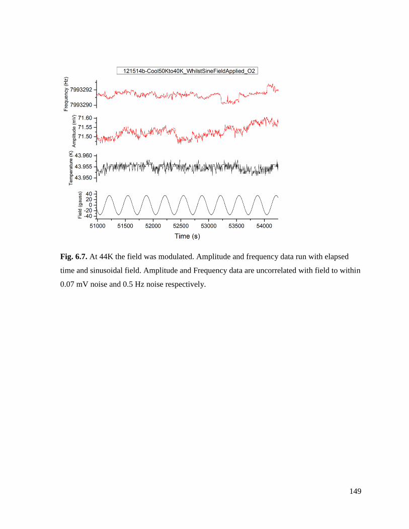
149

Fig. 6.7. At 44K the field was modulated. Amplitude and frequency data run with elapsed

time and sinusoidal field. Amplitude and Frequency data are uncorrelated with field to within

0.07 mV noise and 0.5 Hz noise respectively.

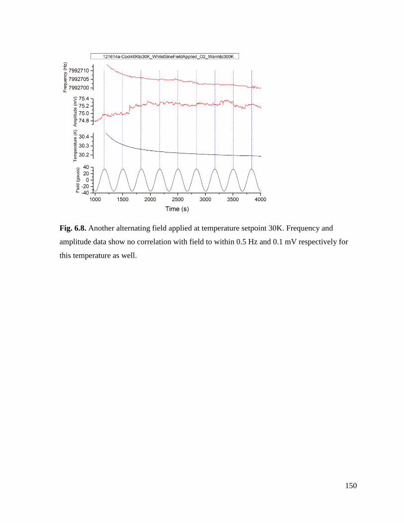
150

Fig. 6.8. Another alternating field applied at temperature setpoint 30K. Frequency and

amplitude data show no correlation with field to within 0.5 Hz and 0.1 mV respectively for

this temperature as well.

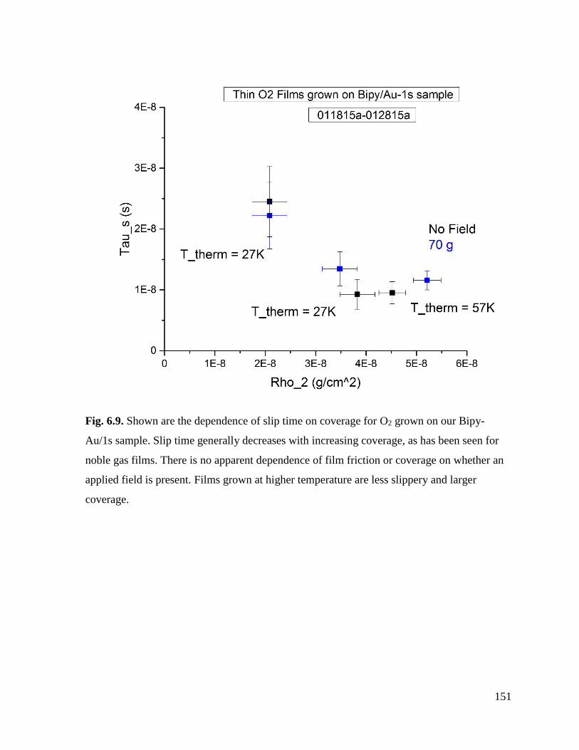
151

Fig. 6.9. Shown are the dependence of slip time on coverage for O2 grown on our Bipy-

Au/1s sample. Slip time generally decreases with increasing coverage, as has been seen for

noble gas films. There is no apparent dependence of film friction or coverage on whether an

applied field is present. Films grown at higher temperature are less slippery and larger

coverage.

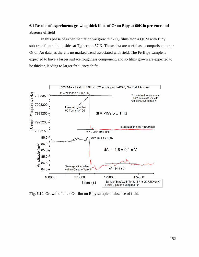
152

6.1 Results of experiments growing thick films of O2 on Bipy at 60K in presence and

absence of field

In this phase of experimentation we grew thick O2 films atop a QCM with Bipy

substrate film on both sides at T_therm = 57 K. These data are useful as a comparison to our

O2 on Au data, as there is no marked trend associated with field. The Fe-Bipy sample is

expected to have a larger surface roughness component, and so films grown are expected to

be thicker, leading to larger frequency shifts.

Fig. 6.10. Growth of thick O2 film on Bipy sample in absence of field.

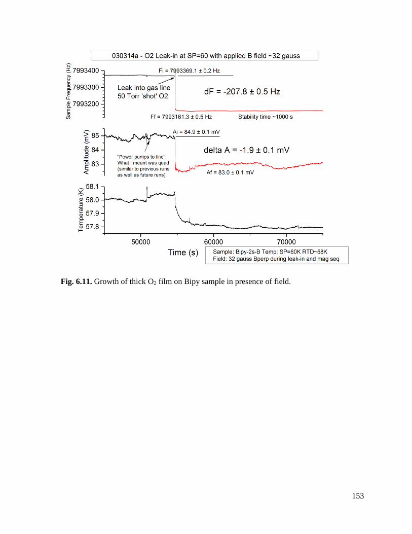
153

Fig. 6.11. Growth of thick O2 film on Bipy sample in presence of field.

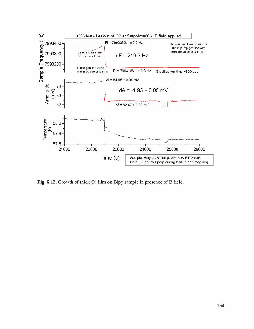
154

Fig. 6.12. Growth of thick O2 film on Bipy sample in presence of B field.

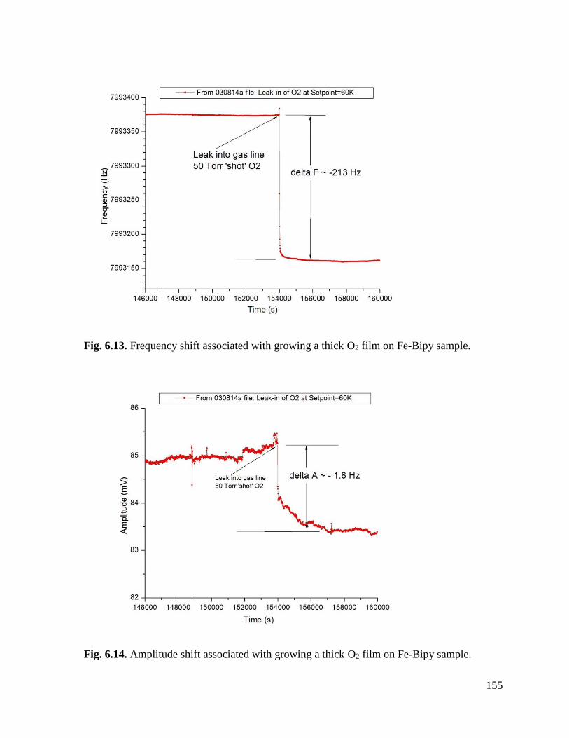
155

Fig. 6.13. Frequency shift associated with growing a thick O2 film on Fe-Bipy sample.

Fig. 6.14. Amplitude shift associated with growing a thick O2 film on Fe-Bipy sample.

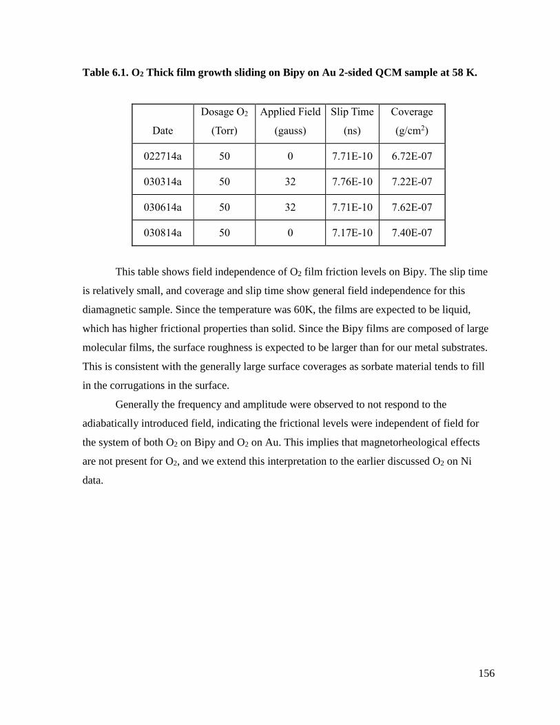
156

Table 6.1. O2 Thick film growth sliding on Bipy on Au 2-sided QCM sample at 58 K.

Date

Dosage O2

(Torr)

Applied Field

(gauss)

Slip Time

(ns)

Coverage

(g/cm2)

022714a 50 0 7.71E-10 6.72E-07

030314a 50 32 7.76E-10 7.22E-07

030614a 50 32 7.71E-10 7.62E-07

030814a 50 0 7.17E-10 7.40E-07

This table shows field independence of O2 film friction levels on Bipy. The slip time

is relatively small, and coverage and slip time show general field independence for this

diamagnetic sample. Since the temperature was 60K, the films are expected to be liquid,

which has higher frictional properties than solid. Since the Bipy films are composed of large

molecular films, the surface roughness is expected to be larger than for our metal substrates.

This is consistent with the generally large surface coverages as sorbate material tends to fill

in the corrugations in the surface.

Generally the frequency and amplitude were observed to not respond to the

adiabatically introduced field, indicating the frictional levels were independent of field for

the system of both O2 on Bipy and O2 on Au. This implies that magnetorheological effects

are not present for O2, and we extend this interpretation to the earlier discussed O2 on Ni

data.

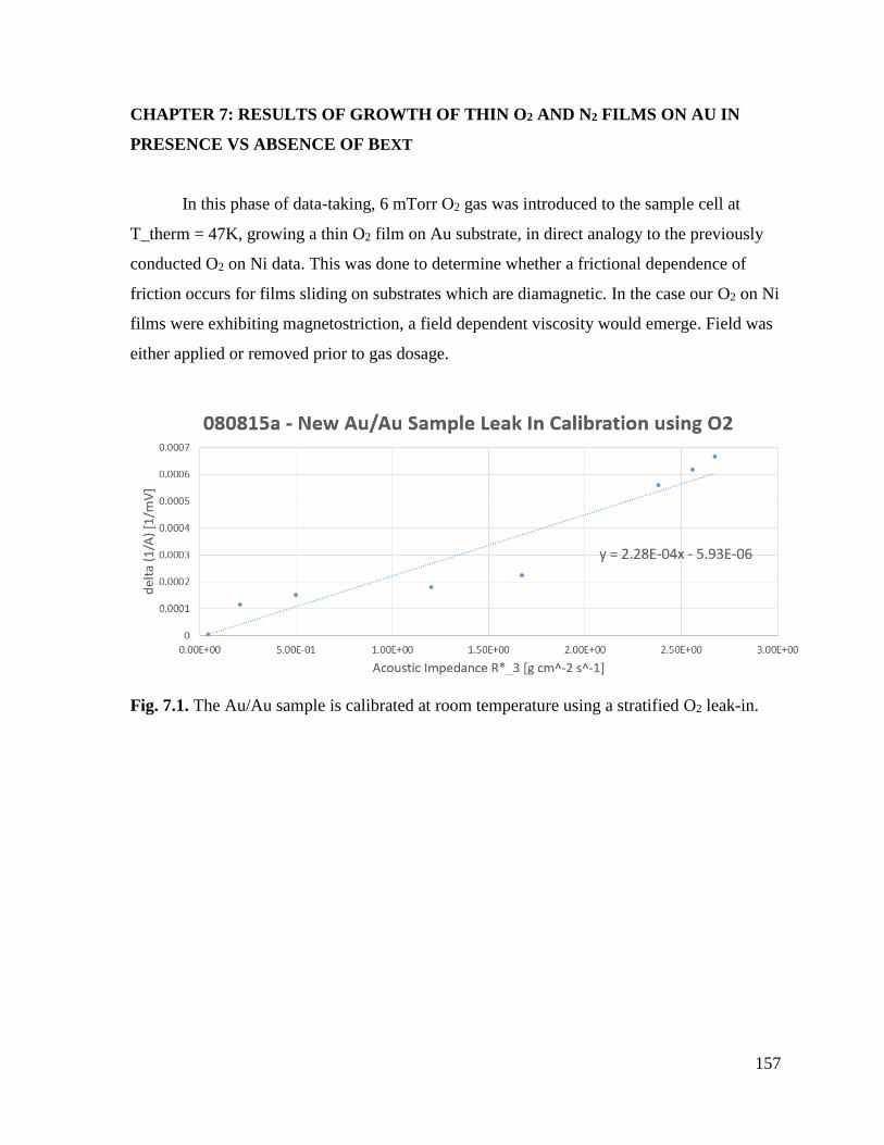
157

CHAPTER 7: RESULTS OF GROWTH OF THIN O2 AND N2 FILMS ON AU IN

PRESENCE VS ABSENCE OF BEXT

In this phase of data-taking, 6 mTorr O2 gas was introduced to the sample cell at

T_therm = 47K, growing a thin O2 film on Au substrate, in direct analogy to the previously

conducted O2 on Ni data. This was done to determine whether a frictional dependence of

friction occurs for films sliding on substrates which are diamagnetic. In the case our O2 on Ni

films were exhibiting magnetostriction, a field dependent viscosity would emerge. Field was

either applied or removed prior to gas dosage.

Fig. 7.1. The Au/Au sample is calibrated at room temperature using a stratified O2 leak-in.

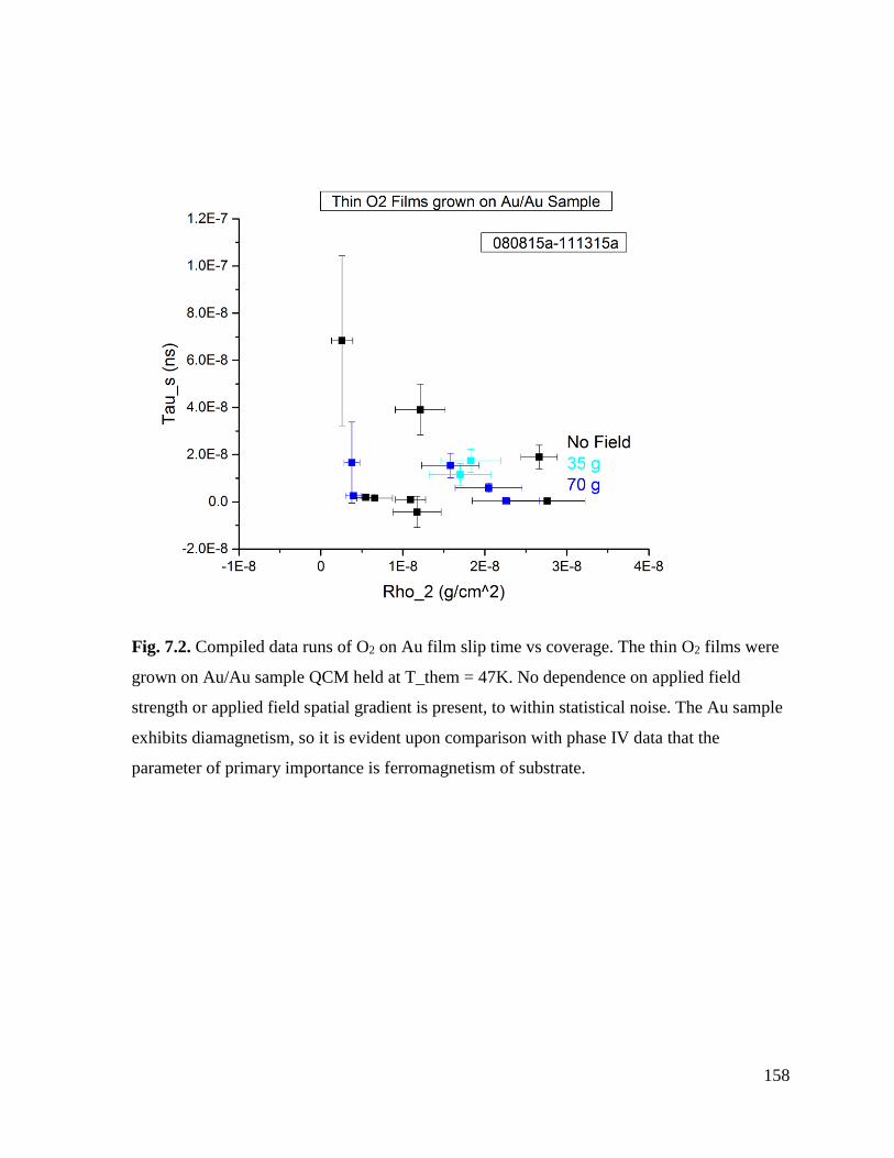
158

Fig. 7.2. Compiled data runs of O2 on Au film slip time vs coverage. The thin O2 films were

grown on Au/Au sample QCM held at T_them = 47K. No dependence on applied field

strength or applied field spatial gradient is present, to within statistical noise. The Au sample

exhibits diamagnetism, so it is evident upon comparison with phase IV data that the

parameter of primary importance is ferromagnetism of substrate.

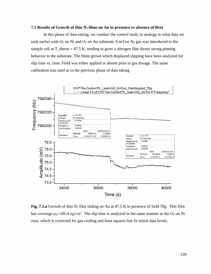
159

7.1 Results of Growth of thin N2 films on Au in presence vs absence of Bext

In this phase of data-taking, we conduct the control study in analogy to what data we

took earlier with O2 on Ni and O2 on Au substrate. 6 mTorr N2 gas was introduced to the

sample cell at T_therm = 47.5 K, tending to grow a nitrogen film shows strong pinning

behavior to the substrate. The films grown which displayed slipping have been analyzed for

slip time vs. time. Field was either applied or absent prior to gas dosage. The same

calibration was used as in the previous phase of data taking.

Fig. 7.3.a Growth of thin N2 film sliding on Au at 47.5 K in presence of field 70g. This film

has coverage ρ2c=20±4 ng/cm2. The slip time is analyzed in the same manner as the O2 on Ni

runs, which is corrected for gas cooling and least squares line fit initial data levels.

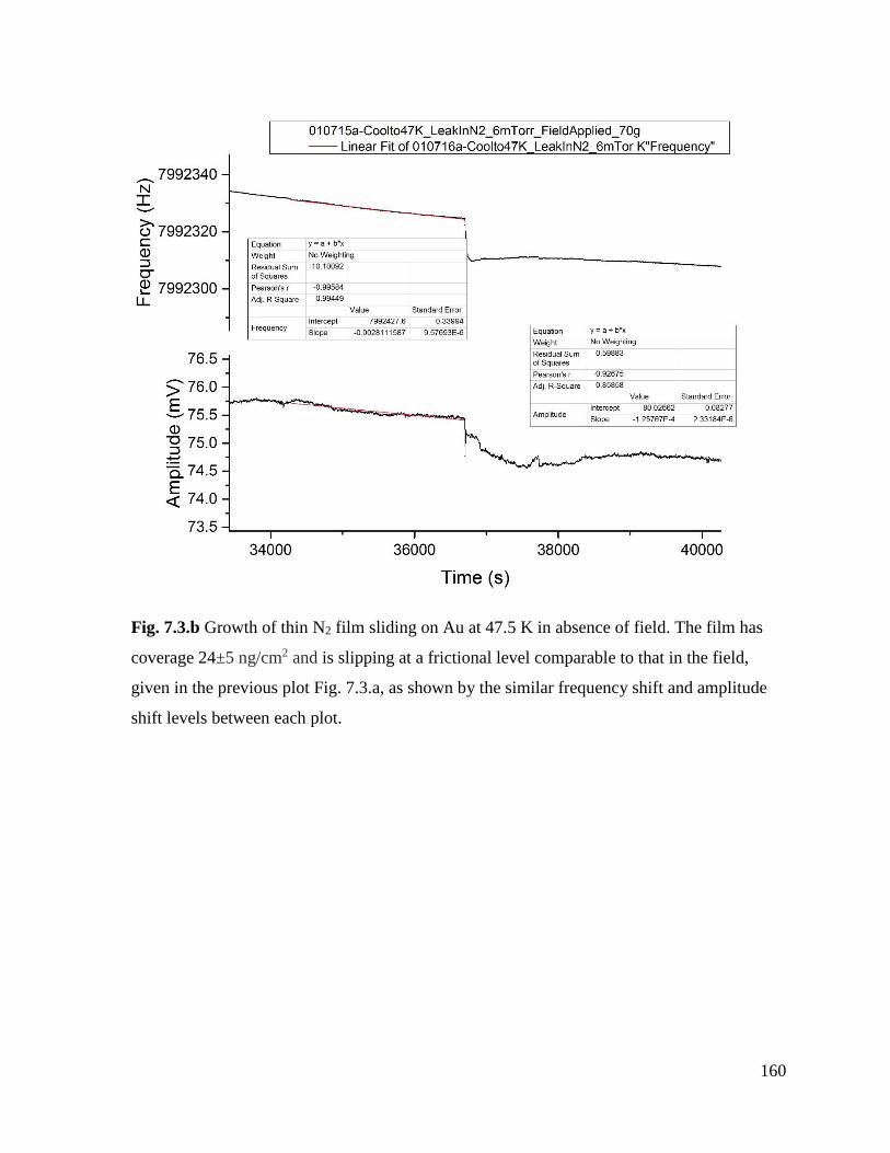
160

Fig. 7.3.b Growth of thin N2 film sliding on Au at 47.5 K in absence of field. The film has

coverage 24±5 ng/cm2 and is slipping at a frictional level comparable to that in the field,

given in the previous plot Fig. 7.3.a, as shown by the similar frequency shift and amplitude

shift levels between each plot.

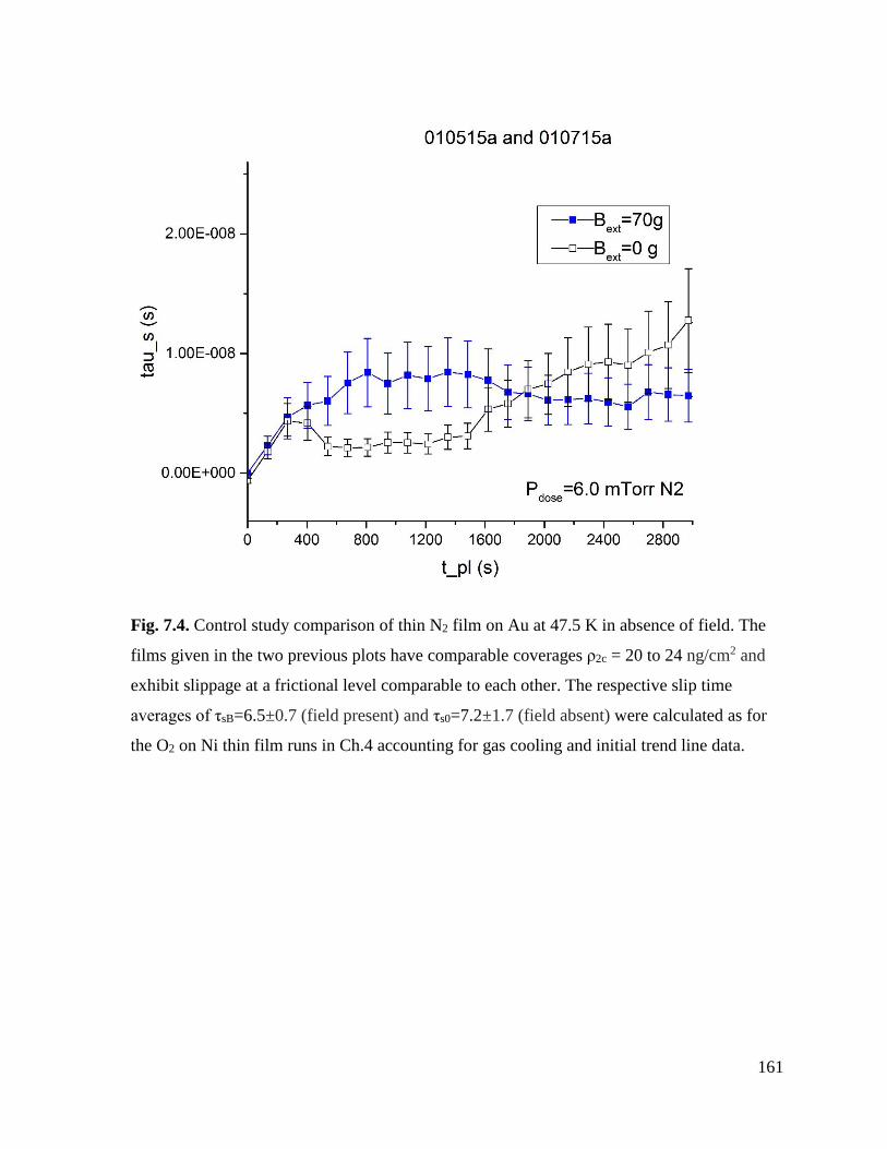
161

Fig. 7.4. Control study comparison of thin N2 film on Au at 47.5 K in absence of field. The

films given in the two previous plots have comparable coverages ρ2c = 20 to 24 ng/cm2 and

exhibit slippage at a frictional level comparable to each other. The respective slip time

averages of τsB=6.5±0.7 (field present) and τs0=7.2±1.7 (field absent) were calculated as for

the O2 on Ni thin film runs in Ch.4 accounting for gas cooling and initial trend line data.

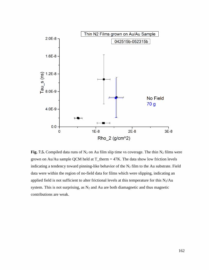
162

Fig. 7.5. Compiled data runs of N2 on Au film slip time vs coverage. The thin N2 films were

grown on Au/Au sample QCM held at T_therm = 47K. The data show low friction levels

indicating a tendency toward pinning-like behavior of the N2 film to the Au substrate. Field

data were within the region of no-field data for films which were slipping, indicating an

applied field is not sufficient to alter frictional levels at this temperature for this N2/Au

system. This is not surprising, as N2 and Au are both diamagnetic and thus magnetic

contributions are weak.

163

7.2. Comparative analysis

Upon comparative analysis of the results of these experiments varying sample

material, dosage gas type, applied field, temperature, and dosage levels, we notice several

trends in the data, foremost being that for thin O2 films sliding on Ni it is evident that an

applied field decreases frictional levels by a factor of two. This phenomenon is not present

for any of the other systems we explored. Each other frictional system we explored involves

at least one element which is either diamagnetic or has a thick film. In addition, and in an

intertwined manner with the magnetic exploration, we have found an increased friction upon

lowering temperature of the O2 thin films on Ni from 47K through 30K, indicating a change

in phase from fluid to δ, and a resultant increase in frictional levels.

In film-substrate frictional systems magnetic in nature, several dissipation

mechanisms arise as candidates. To explain the interplay between these findings, we here

consider the mechanism pathways expected to be present to varying degrees at various

coverages, fields, temperatures and system material types. These candidate mechanisms we

refer to as magnetostriction, spin friction, and magnetorheology, and we attribute this finding

in O2 on Ni data to magnetostrictive effects. Our findings are summarized in the table in

Ch.8.

The magnetostriction explains our increase in slip time for O2/Ni at 47K, as well

explaining the pinning behavior in absence of field in the incrementally cooled system. Also,

the relatively small effect of changing the field once the films have established equilibrium

suggests the state is locked, indicating a magnetostriction effect. The similarity of average

values of slip time between field present and absent for the O2/Au and O2/Fe-Bipy/Au as

well as N2/Au implies magnetorheology does not observably impact their friction levels. This

allows us to filter the mechanism out of the O2/Ni and O2/Cooling data. Spin friction was not

observed in any of the systems experimented on, to within frictional dependence on

temperature.

Of primary interest, from comparison of data between ferromagnetic and diamagnetic

samples emerges a dependence of slip time on applied field strength – films grown in

presence of field are about 1.6 times as slippy as the same films grown in the field absent

condition. This dependence emerges in the case of thin fluid oxygen films adsorbed at 47K.

The effect is seen to a lesser extent in thick oxygen films, and is absent for films of any

164

thickness O2 on the Bipy and Au substrates, as well as N2 on Au. Of all candidate

mechanisms, we attribute this finding to oxygen’s molecular axis aligning in the field at the

fluid-ζ phase transition, thus influencing friction levels through changes in adsorbate-

substrate corrugation potential.

These experiments have also found temperature dependence and coverage

dependence of slip time values for films sliding on these substrates. The comparison allows

us to elucidate the primary mechanisms of dissipation occurring in the film-substrate

systems.

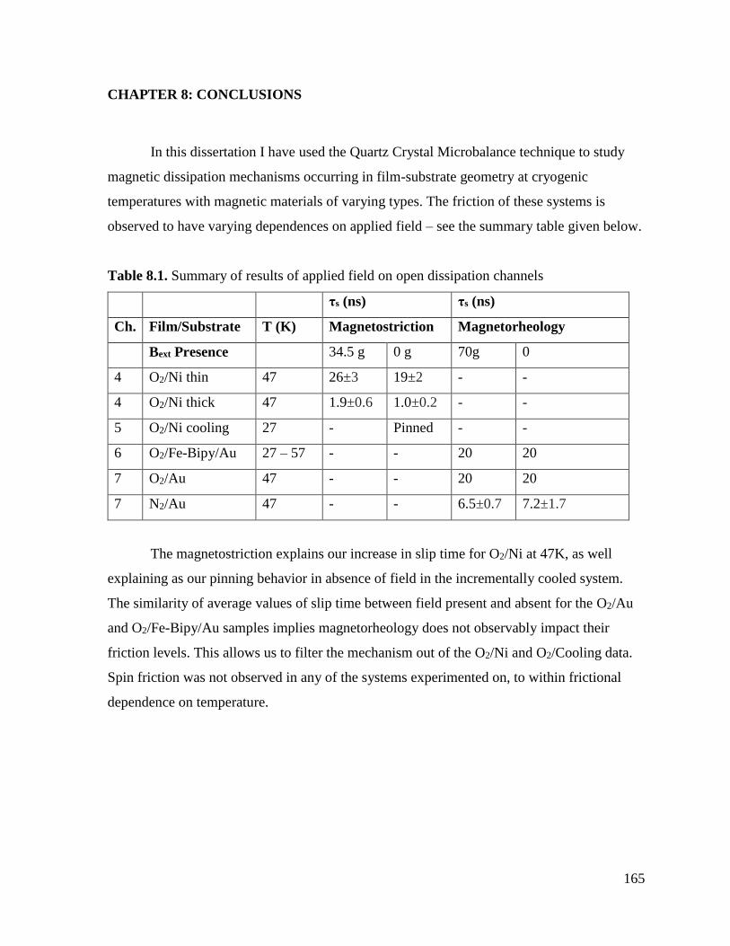
165

CHAPTER 8: CONCLUSIONS

In this dissertation I have used the Quartz Crystal Microbalance technique to study

magnetic dissipation mechanisms occurring in film-substrate geometry at cryogenic

temperatures with magnetic materials of varying types. The friction of these systems is

observed to have varying dependences on applied field – see the summary table given below.

Table 8.1. Summary of results of applied field on open dissipation channels

τs (ns) τs (ns)

Ch. Film/Substrate T (K) Magnetostriction Magnetorheology

Bext Presence 34.5 g 0 g 70g 0

4 O2/Ni thin 47 26±3 19±2 - -

4 O2/Ni thick 47 1.9±0.6 1.0±0.2 - -

5 O2/Ni cooling 27 - Pinned - -

6 O2/Fe-Bipy/Au 27 – 57 - - 20 20

7 O2/Au 47 - - 20 20

7 N2/Au 47 - - 6.5±0.7 7.2±1.7

The magnetostriction explains our increase in slip time for O2/Ni at 47K, as well

explaining as our pinning behavior in absence of field in the incrementally cooled system.

The similarity of average values of slip time between field present and absent for the O2/Au

and O2/Fe-Bipy/Au samples implies magnetorheology does not observably impact their

friction levels. This allows us to filter the mechanism out of the O2/Ni and O2/Cooling data.

Spin friction was not observed in any of the systems experimented on, to within frictional

dependence on temperature.

166

In the O2 on Ni experiments we observed a significantly decreased friction, by a

factor of 1.6, for thin films at 47K. This observation was seen to a lesser extent in thick films

implying it was an interfacial effect. At this point several dissipation channels arose as

candidates which are observed in previous experiment and shown in previous theory to occur

in similar systems. We proposed as an explanation of the decreased friction in field behavior:

spin friction, magnetostriction and magnetorheology mechanisms. We then tuned further

parameters to elucidate the effect of these frictional channels. These parameters were

temperature from 47K to 26K and to 57K, adsorbate film thickness, substrate composition

from Ni to Au and to Bipy, applied field from 0 to 70 g, and adsorbate composition from O2

to N2.

It was found by our subsequent experimentation upon entering the δ phase that

frictional enhancement took place, implying slip time dependence on orientation of the

oxygen molecules. It is from this observation clear that the field in our previous data had an

impact on frictional levels by means of molecular orientation in the field, and thus the ζ

phase.

We observed, controlled and accounted for the magnetostriction present in 2D oxygen

films by means of an applied field - this finding represents a first step towards external

control of frictional interactions within a film-substrate interface by way of magnetic degrees

of freedom.

Thick films studied here had a lower slip time in comparison to thin – general to substrate as

well as adsorbate. Additionally, the magnetorheological effect in liquid oxygen, proposed by

Boulware [1], is not observable by the QCM technique with thin and thick films sliding on

Au and Bipy.

To the previously outstanding questions listed at the end of chapter 2, this work

brings answers:

A. The Altfeder [2] and Highland [3] studies, as well as the Mistura [4,5] studies showed

that a magnetic field could alter the superconductivity state then alter friction indirectly. This

work shows that friction can be altered in non-superconducting systems by means of a

magnetic field.

167

B. The Mistura studies required a thermal annealing to record friction measurements at

cryogenic temperatures. This constraint is not in our system required to attain data which is

reliably reproducible without the thermal annealing.

C. In the Wiesendanger [6,7] studies, a new microscopy technique was invented that

relies on magnetic dissipation of a tip in contact with a magnetic substrate – Previously no

experiment has determined whether this dissipation carries over into two dimensions.

D. The Johannesmann [8] experiment observed magnetorheological fluid’s dissipation

being altered by a field. The amplitude shift can in general be interpreted as a shift in the

resistance. Magnetorheological effects were not seen to be present, or at least not dominant

for our oxygen system, as had been an open question previously.

E. MExFM [9] have shown spin contrast superimposed on vdW lattice. In the

framework of Cieplak [10], does this affect the friction of a film’s sliding in a way that is

observable? We found increased frictional levels for a system with decreased temperature.

This system’s temperature decrease to 30K results in an increased susceptibility, thus an

increased locking to nearby exchange energies. The prediction for spin friction is towards

decreased friction for increased locking, opposite to what was observed.

F. The Kadau study [11] predicted that the magnetic damping would be observable in

2D systems but this has yet to be shown experimentally. This dissertation represents a first

observation and characterization of magnetic damping mechanisms in thin oxygen films.

G. Cai [12] conducted simulations of a magnetic monolayer on a magnetic substrate find

a decreased total friction, due to the spin friction. This behavior has yet to be experimentally

observed, especially to find whether the behavior changes in the case the adsorbate

magnetism is not rigidly locked (as in the Wiesendanger tip studies). We found the behavior

to not be dominant when the magnetic degrees of freedom are not rigidly locked. If the

magnetic degrees of freedom are considered rigid, the adsorbate molecule complies with a

decreased interaction corrugation with the substrate due to repulsive exchange.

168

H. The studies on oxygen adsorption on graphene [13-15] and metals [16-19] point to

the ability to alter the molecular orientation. The primary result of this dissertation found the

phase structure carries over to frictional behaviors – increased friction in the δ phase,

intermediate friction in the fluid phase, and decreased friction levels in the ζ phase induced

by an applied field.

169

REFERENCES CHAPTER 8

[1] Boulware, J. C. (2010). Experiment and Simulation on the Dynamics of a Slug of Liquid

Oxygen Displaced by a Pulsed Magnetic Field. (Doctoral dissertation). Retrieved from:

http://digitalcommons.usu.edu/etd.

[2] Altfeder, I., & Krim, J. (2012). Temperature dependence of nanoscale friction for Fe on

YBCO. Journal of Applied Physics, 111, 094916. http://doi.org/10.1063/1.4717983

[3] Highland, M., & Krim, J. (2006). Superconductivity Dependent Friction of Water,

Nitrogen, and Superheated He Films Adsorbed on Pb(111). Physical Review Letters,

96(June), 226107. http://doi.org/10.1103/PhysRevLett.96.226107

[4] Bruschi, L., Fois, G., Pontarollo, a., Mistura, G., Torre, B., Buatier De Mongeot, F., …

Valbusa, U. (2006). Structural depinning of Ne monolayers on Pb at T<6.5K. Physical

Review Letters, 96(June), 2–5. http://doi.org/10.1103/PhysRevLett.96.216101

[5] Bruschi, L., Pierno, M., Fois, G., Ancilotto, F., Mistura, G., Boragno, C., … Valbusa, U.

(2010). Friction reduction of Ne monolayers on preplated metal surfaces. Physical Review B

- Condensed Matter and Materials Physics, 81, 1–5.

http://doi.org/10.1103/PhysRevB.81.115419

[6] Wolter, B., Yoshida, Y., Kubetzka, A., Hla, S. W., Von Bergmann, K., & Wiesendanger,

R. (2012). Spin friction observed on the atomic scale. Physical Review Letters,

109(SEPTEMBER), 1–5. http://doi.org/10.1103/PhysRevLett.109.116102

[7] Ouazi, S., Kubetzka, A., von Bergmann, K., & Wiesendanger, R. (2014). Enhanced

Atomic-Scale Spin Contrast due to Spin Friction. Physical Review Letters, 112, 076102.

[8] Rodriguez-López, J., Castro, P., de Vicente, J., Johannsmann, D., Elvira, L., Morillas, J.,

& Montero de Espinosa, F. (2015). Colloidal Stability and Magnetic Field-Induced Ordering

of Magnetorheological Fluids Studied with a Quartz Crystal Microbalance. Sensors, 15,

30443–30456. http://doi.org/10.3390/s151229808

[9] Kaiser, U., Schwarz, a., & Wiesendanger, R. (2007). Magnetic exchange force

microscopy with atomic resolution. Nature, 446(March), 522–525.

http://doi.org/10.1038/nature05617

[10] Cieplak, M., Smith, E. D., & Robbins, M. (1994). Molecular Origins of Friction : The

Force on Adsorbed Layers, 265(5176), 1209–1212.

[11] Kadau, D., Hucht, A., & Wolf, D. E. (2008). Magnetic friction in Ising spin systems.

Physical Review Letters, 101(September), 1–4.

http://doi.org/10.1103/PhysRevLett.101.137205

170

[12] Cai, X., Wang, J., Li, J., Sun, Q., & Jia, Y. (2016). Spin friction between Co monolayer

and Mn/W(110) surface: Ab Initio investigations. Tribology International, 95, 419–425.

http://doi.org/10.1016/j.triboint.2015.11.037

[13] Marx, R., & Christoffer, B. (1985). Magnetocaloric effects of 2D adsorbed O2. Journal

of Physics C: Solid State Physics, 18, 2849–2858. http://doi.org/10.1088/0022-

3719/18/14/016

[14] Bhethanabotla, V. R., & Steele, W. a. (1987). Molecular dynamics simulations of

oxygen monolayers on graphite. Langmuir, 3, 581–587. http://doi.org/10.1021/la00076a025

[15] Bhethanabotla, V.R., & Steele, W. (1987). Simulations of O2 adsorbed on graphite at

45K: the monolayer to bilayer transition. Can. J. Chem. 66, 866.

[16] Kurahashi, M., Sun, X., & Yamauchi, Y. (2012). Magnetic properties of O2 adsorbed on

Cu(100): A spin-polarized metastable He beam study. Physical Review B - Condensed

Matter and Materials Physics, 86, 1–2. http://doi.org/10.1103/PhysRevB.86.245421

[17] Yamagishi, S., Jenkins, S. J., & King, D. a. (2003). First principles studies of

chemisorbed O on Ni{1 1 1}. Surface Science, 543(April), 12–18.

http://doi.org/10.1016/j.susc.2003.08.002

[18] Aoki, M., Taoka, H., Kamada, T., & Masuda, S. (2001). Local electronic states of

oxygen on Ni(111) surface studied by metastable atom electron spectroscopy. Journal of

Electron Spectroscopy and Related Phenomena, 114-116 (2001) 507-512

[19] Kazama, Y., Matsumoto, M., Sugimoto, T., Okano, T., & Fukutani, K. (2011). Low-

temperature surface phase and phase transition of physisorbed oxygen on the Ag(111)

surface. Physical Review B - Condensed Matter and Materials Physics, 84(April), 4–6.

http://doi.org/10.1103/PhysRevB.84.064128

171

APPENDIX

172

APPENDIX A

Calculation of uncertainty in coverage and slip time calculations

For the slip time vs time plots of data, the slip time for each field and coverage

condition was calculated at each 10 second time step post-leak-in by using equation given in

chapter 3:

𝜏 = 𝑅∗

𝜔𝑋∗=

1𝑚 ((

1𝐴𝑓

) − (1𝐴𝑖

) − 𝑏)

𝜔2 (−2.221 ∗ 105 (𝑓𝑓 − 𝑓𝑖

𝑓02 ))

(A.0)

which requires as inputs initial and final values of both frequency and amplitude. Frequency

and inverse amplitude shifts were calculated at each time step by subtracting the frequency or

inverse amplitude value at that time step from the original frequency or inverse amplitude

level before the film was grown, accounting for linear trends and gas cooling.

The mean slip time and error bars for each field condition were calculated at each

time step by averaging over each run the slip time values at that time step and calculating the

standard deviation of the mean. In the table, the slip time measurement values correspond to

best estimate and uncertainty. The best estimate slip time value was calculated for each

condition by averaging over all time steps in the window from 20 to 30 minutes post-leak-in

the mean of slip time values for runs with that condition. The uncertainty values are the

average calculated over all time steps in this time window of the values for standard

deviation of the mean. To calculate for example the thin O2 on Ni runs the ratio of slip times:

𝑞 =

𝜏𝐵

𝜏0=

26

19= 1.4

(A.1)

We calculate the fractional uncertainty by adding in quadrature the fractional uncertainty of

slip times for field present and absent:

𝛿𝑞

|𝑞|= √(

3

26)

2

+ (2

19)

2

= 0.156 ⇒ 𝛿𝑞 = (26/19) ∗ 0.156 = 0.213

(A.2)

So our measured value of the ratio is, accounting for significant figures:

𝜏𝐵

𝜏0= 1.4 ± 0.2. (A.3)

173

The fractional uncertainty in a given measurement of slip times is expressed as a sum

in quadrature of fractional uncertainty in impedance and coverage:

𝛿𝜏

|𝜏|= √(

𝛿𝑅2∗

|𝑅2∗|

)

2

+ (𝛿𝜌2

|𝜌2|)

2

(A.4)

Where fractional uncertainty in coverage δρ2 is:

𝛿𝜌2

|𝜌2|=

𝛿(Δ𝑓)

|Δ𝑓|

(A.5)

Where Δ𝑓 is the frequency shift between the initial trend-line 𝑓𝑖 and the corrected value:

𝑓′ = 𝑓𝑓 + Δ𝑓𝑔𝑐 + 𝑓𝑓𝑡 . (A.6)

The 𝑓𝑓 are frequency data after film growth is initiated at time post-leak-in 𝑡𝑝𝑙 = 0. Δ𝑓𝑔𝑐 is

the frequency shift associated with the sample cooling of 0.049 ± 0.003 K which is calibrated

to 3.3 ± 0.1 Hz for our thin film data grown in 7mTorr O2 dosage levels. For thick films at

higher dosage pressures 100 mTorr and above, the uncertainty in sample temperature

dependence of frequency contributes; this is taken to be the value of deviation in slopes

among the runs with the same sample, within the range 68 to 85 Hz/K at 47.5K. The other

significant contributor to thick film coverage uncertainty is uncertainty of temperature shift

δ(ΔT) in a given sample. Temperature shifts upon leak-in are 0.388 ± 0.03 K at high dosage.

The time dependence is extrapolated to 𝑓𝑓𝑡 = −𝑚𝑓𝑡 ∗ 𝑡𝑝𝑙, where 𝑚𝑓𝑡 is least-squares fit

calculated for data 3600s prior to leak-in initiation and has values calculated in the range

10−5 𝑠−1. The regime 𝑡𝑝𝑙>3000𝑠 at low coverage the product 𝛿𝑚𝑓𝑡 ∗ 𝑡𝑝𝑙 approaches 10% of

the total frequency shift – for this reason we confine our analysis to times within 500s-3000s

window. Since the final frequency is given by corrections from the trend-line fit and gas

cooling, its deviation can be written, for thin film case:

δ(Δ𝑓) = √𝜎𝑓𝑖

2 + 𝜎𝑓𝑓

2 + 𝜎𝑓𝑇2

(A.7)

The standard deviation in initial (final-fit) frequency data from the trend-line are given by 𝜎𝑓𝑖

and 𝜎𝑓𝑓 within time steps of 1000s – typically the values are 0.5 to 0.6 Hz. Here we have

attributed uncertainty in cooling to 𝛿(Δ𝑓𝑔𝑐) = 𝜎𝑓𝑇, accounting for the width of the linear fit

of frequency with temperature, and the same for 𝜎𝑓𝑖> 𝑑𝑚𝑓𝑡 ∗ 𝑡𝑝𝑙 for short times (within

174

3600s). For thick films, there is an extra term added in quadrature to account for the

uncertainty in the δ(𝑚𝑓𝑇Δ𝑇) term.

Similarly for the amplitude value:

𝐴′ = 𝐴𝑓 + Δ𝐴𝑔𝑐 + 𝐴𝑓𝑡 . (A.8)

Where 𝐴𝑓 is the post-leak-in amplitude data, Δ𝐴𝑔𝑐 is amplitude shift due to gas cooling and

𝐴𝑓𝑡 line fit subtraction. For the low-dosage runs Δ𝐴𝑔𝑐 < 0.01 𝑚𝑉 is negligibly small. The

uncertainty in the corrected amplitude values are therefore, for thin films:

δ𝐴′ = √𝜎𝐴𝑓

2 + 𝜎𝐴𝑇2

(A.9)

where the 𝜎𝐴𝑓 and 𝜎𝐴𝑇 are the standard deviations in the post-leak in amplitude data and

amplitude to temperature line fit respectively. These amplitude and frequency data give our

acoustical impedance via:

𝑅2

∗ =1

𝑚{

1

𝐴′−

1

𝐴𝑖} − 𝑏,

(A.10)

The uncertainty of which is dominated by two terms:

𝛿𝑅2∗ = 𝑞𝑚√(

𝛿𝑞

|𝑞|)

2

+ (𝛿𝑚

|𝑚|)

2

.

(A.11)

Where q is the quantity given in brackets.