International Journal of Material Forming manuscript No.(will be inserted by the editor)

A two-pronged approach for springback variability assessmentusing sparse Polynomial Chaos Expansionand multi-level simulations

Jérémy LEBON · Guénhaël LE QUILLIEC · Piotr BREITKOPF ·Rajan FILOMENO COELHO · Pierre VILLON

Received: date / Accepted: date

Abstract We show in this study that stochastic analy-sis of metal forming process requires both a high preci-sion and low cost numerical models in order to take intoaccount very small perturbations on inputs (physical aswell as process parameters) and to allow for numerousrepeated analysis in a reasonable time.

To this end, an original semi-analytical Bending-Under-Tension model is used to accurately predict theinfluence of small random perturbations around a nom-inal solution estimated with a full scale Finite ElementModel (FEM). We introduce a custom sparse variant ofthe Polynomial Chaos Expansion (PCE) to model thepropagation of uncertainties through this model at lowcomputational cost. Next, we apply this methodologyto the deep drawing process of U-shaped metal sheetconsidering up to 8 random variables.

Keywords Springback variability assessment ·sparse Polynomial Chaos Expansion · semi-analyticalBending-Under-Tension model

1 Introduction

In order to accurately assess the springback variabilityof a formed metal sheet one has to take into account un-certainties linked with the deep drawing process (clampforces, tool radius tolerances, punch celerity, etc.) as

J. LEBON · G. LE QUILLIEC · P. BREITKOPF · P. VIL-LONLaboratoire Roberval, UMR 7337, Université de Technologiede Compiègne, BP 20529, 60205 Compiègne cedex, FRANCETel.: +33 (0)3 44 23 46 63E-mail: jeremy.lebon@utc.fr

J. LEBON · R. FILOMENO COELHOUniversité Libre de Bruxelles (ULB), BATir Department CP194/2, 50, avenue Franklin Roosevelt, B-1050 Brussels (BEL-GIQUE)

well as those linked with the physical model parameters(material properties, thickness of the metal sheet, etc.).The assessment of the after-springback shape variabil-ity relies on the combination of two numerical tools:a numerical model of the deep drawing process and astochastic process to propagate the uncertainties intothis model.

In the context of variability study, the numericalmodel has to be computed for very small variationsof the input parameters. Comparing the model errorwith the variation magnitude of the output function isof paramount importance to ensure the validity of thevariability study. The Finite Element Method (FEM) isa standard tool to construct the underlying numericalmodel: [16] uses FEM to perform sensitivity analysison springback of sheet metal forming, [12] uses FEMcomputations coupled to classical reliability methodol-ogy to perform reliability analysis of the deep draw-ing process. However, the FEM shows important limi-tations regarding the variability issues. First of all, tomodel the highly non-linear phenomena involved (largestrains, plasticity, frictional contact, etc.) with a highenough accuracy for small variations of the input pa-rameters, the model has to be refined in every direc-tion (decreasing the mesh size and increasing the num-ber of Gauss points). This rapidly leads to unaffordablecomputational costs, specially when a high number ofcalls is needed. To circumvent this cost issue, alterna-tive approaches have been proposed: [18] in a sensi-bility analysis context uses an analytical model of thespringback, [15] proposes a “one step” inverse approachfor the analysis and optimum process design of deepdrawn industrial metal part, [3] uses this approach inan optimizaiton context to train a Moving Least Squaresurrogate to efficiently perform the optimization. A sec-ond limitation is that FEM generates intrinsic errors

2 Jérémy LEBON et al.

such as a discretization error (due to mesh size) andcomputational errors (round-off, quadrature, ...) [11].The authors in [14] show that, contact description andthrough-thickness integration may play a leading role.

Common computational methods propagate the un-certainties defined on the random parameters to theshape of the formed metal sheet based on a sampling ofthe random input parameters (Monte Carlo simulation,Importance Sampling, etc.) and thus require a relativelyhigh number of calls to the underlying computationalmodel. The authors in [18] use Monte Carlo simula-tions to perform a sensitivity analysis of the springbackwith regards to process parameters, [12] and [17] useFORM methodology coupled with an enhanced adap-tive Monte Carlo methodology to assess the reliabil-ity of the deep drawing process. The use of stochasticmetamodels combined with advanced sampling meth-ods offers an alternative to the crude sampling meth-ods. In [10] the authors propose the use of linear andquadratic response surface combined with Monte CarloSimulation to perform the reliability assessment of sheetmetal forming process. In [5], a second order Polyno-mial Chaos Expansion (PCE) is used as a stochasticresponse surface to assess the reliability of the formedmetal sheet with regards to tolerance criteria. Howewer,in these studies, the number of random variables takeninto account by the stochastic response surface is lim-ited.

In this paper, we propose an original two-prongedapproach to accurately propagate the uncertainties intoa “high resolution” model at low computational cost.Our approach is based on a combination of a stochasticsurrogate (PCE) and a physics Reduced Order Model(ROM). We show by the observation, that in the caseof variability study, as the order of magnitude of thevariation range decreases the full scale model predic-tion becomes unstable. We investigate then regulariza-tion features of a “high resolution” physics based ROM,allowing us to reach numerical stability for smaller vari-ations of the input variables. Then, a stochastic surro-gate model is trained on the full parameter variationrange and it is then used to perform the variabilitystudy at low computational cost.

In the second section, we introduce the PolynomialChaos Expansion (PCE) as a stochastic response sur-face for the uncertainty propagation. We highlight theneed, of a numerical model characterized by a high pre-cision for small perturbations of the input variablesas well as low computational cost. The third sectionquantifies the limitations of the FEM modeling withregards to the variability problematic by considering“very” small variations of the input parameters arounda nominal value. The two following sections introduce

the ingredients of the proposed approach: the semi-analytical (FEM based) Bending-Under-Tension (B-U-T) model and the sparse custom version of the PCE(inspired from [2]) for an enhanced accuracy of the vari-ability study at low computational cost. The fourth sec-tion introduces the semi-analytical B-U-T and showshow it allows to alleviate the FEM limitations by sidestepping the main numerical noise sources (contact de-scription and through-thickness integration). The fifthsection discusses a custom sparse version of the PCE,putting into evidence the need to create a sparse poly-nomial chaos expansion when the number of randomvariables is increasing. Finally, the sixth section of thepaper illustrates the methodology on the deep drawingprocess of U-shaped metal sheet with 8 random vari-ables to assess the variability of the springback shapeparameters considering a relatively large number of ran-dom variables chosen among the most influential ones[16,5].

2 Assessing the springback variability usingPolynomial Chaos Expansion

The PCE is a stochastic metamodel, that is intendedto give an intrinsic representation of the stochasticbehavior of a functional Y (scalar random variable)that is defined as a function of an input random vectorΞ = {ξ1, ξ2, . . . , ξM} with M coordinates and withprescribed probability density function fΞ(Ξ) [7].Its accuracy to predict the variability of the outputfunction Y highly depends on the underlying “highfidelity model”.

2.1 Building the multi-variate Hermitian PCE

Assuming that Ξ has independent Gaussian compo-nents and that the functional Y is a second order ran-dom variable (E(Y 2) < ∞), then according to the Ca-meron Martin Theorem, generalized in M dimensions([4]) an exact PCE of the functional Y is given by

Y (Ξ) =

∞∑j=0

γjΨj(Ξ), (1)

where the {Ψj(Ξ), j = 0, 1, . . . ,∞} are the multivari-ate polynomials orthogonal with respect to the naturalinner product

< Ψk, Ψl >=

∫Ψk(Ξ)Ψl(Ξ)

M∏i=1

fξi(ξi)dξi (2)

Title Suppressed Due to Excessive Length 3

with fξi(ξi) the marginal distribution of the ith com-ponent of the random vector Ξ.

For M independent Gaussian random variables,multi-variate Hermitian polynomials exhibit thisorthogonality property. Given a degree N , the multi-variate set of MN+1 Hermitian polynomials are builtusing the tensor product of mono-variate hermitianpolynomials. Practically, only a finite P < MN+1

number of terms is retained yielding to the reducedexpansion

Y (Ξ) ≈P−1∑j=0

γjΨj(Ξ), (3)

where

P =(N +M)!

N !M !. (4)

In order to properly interpret the sparse PCE algo-rithm, an appropriate scheme for numbering the multi-variate polynomials of degree d ≤ N needs to be intro-duced. Considering the jth multi-variate polynomial, wenote that expressing j in base N + 1 (with M digits)gives j = dj1×M0+dj2×M1+ ...+djM×MN . Each digit0 ≤ djm ≤ N , m = 1, . . . ,M may be interpreted as thedegree of the mono-variate polynomial evaluated withthe mth variable. The product of the M mono-variatepolynomials of degree dj1, d

j2, ..., d

jM yields to the corre-

sponding jth multi-variate polynomial whose degree is∑Mi=0 di. The numbering algorithm may then proceed

as follow:

1. Generate a full set of indices S = {0, 1, . . . ,MN+1}in base N + 1 (with M digits).

2. Retain only the subset set of indices S∗ for which∑Mi=0 di ≤ N .

3. Renumber the polynomials from 0 to P − 1 (Eq.4).

2.2 Computing the coefficients of the multi-variatePCE

The PCE accuracy highly depends on the precise com-putation of its P coefficients. An intrusive Galerkin typeapproach has been first proposed by [7]. Projectionsbased non-intrusive methods take benefit from the or-thogonal properties of the multivariate polynomials ofthe expansion.Equivalent stochastic collocation is basedon a Lagrangian interpolation in the stochastic space[20]. These methods are the most accurate but also themost greedy and become rapidly unaffordable in highdimensions.

The regression based approach (on which wefocus on this paper) consists in solving the follow-ing overdetermined system of equations, where eachΞ(i), i ∈ {1, ..., Q} represent Q > P samples of therandom vector Ξ. The optimal number of realizationsneeded to assess the coefficients with a good accuracyis still an open research area, but an empirical ruleproposes Q ≥ 2± 3× P [1].

Y (Ξ(1))

...Y (Ξ(Q))

︸ ︷︷ ︸Y

=

Ψ0(Ξ(1)) . . . ΨP−1(Ξ

(1))...

...Ψ0(Ξ

(Q)) . . . ΨP−1(Ξ(Q))

︸ ︷︷ ︸

Ψ

γ0...

γP−1

︸ ︷︷ ︸γ

(5)

This overdetermined system of equations may be solvedusing a singular value decomposition of the Ψ matrix.

Once the set of P coefficients {γ0, ..., γP − 1} hasbeen determined, one may compute the statistical mo-ments of Y analytically avoiding Monte Carlo simula-tions. The first two moments are given by:

E(Y ) =γ0 (6)

σ2(Y ) =

P−1∑j=1

E(Ψ2j )γ

2j (7)

For an accurate assessment of the statistical mo-ments, a special attention has then to be given to thecomputations of the P coefficients (Eq.7). Thus, accord-ing to Eq.5, the underlying model has then to be asaccurate as possible. Moreover, computing the wholeset of coefficients may require a high number of callsQ = 2− 3×P to the underlying model as P (Eq.4) in-creases exponentially with the number of variables Mand the degree N .

In the following section we introduce a test case andwe quantify the precision requirements for the simula-tion model. We show that using typical FEM simula-tions may lead to inaccurate results for a reasonablecomputational cost when small perturbations are in-volved.

3 Inpact of through-thickness integration onthe springback prediction

3.1 Test case

To illustrate the issue of model variability with regardsto small perturbations, we choose to model a 2D deepdrawn U-shaped metal sheet. The springback affectingthe formed part is measured using the following shape

4 Jérémy LEBON et al.

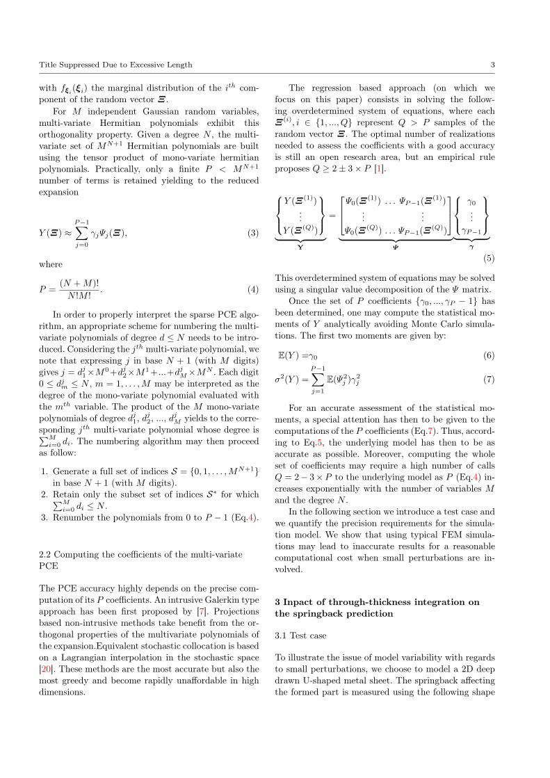
parameters, the curvature ρ and the angles β1 and β2defined as illustrated in Fig.1.

β

β

Fig. 1 Springback parameters

For small blank thickness variations from 0.6 mmand 1 mm (with an incremental step of 0.04 mm), a setof simulations is run.

The whole simulation process (deep drawing andspringback) has been performed using a legacy soft-ware [9] with the following hypothesis. The deep draw-ing phase has been modeled using a dynamic explicitapproach as material non linearities are involved. Thespringback phase is modeled using a static approach asit cor-responds to an elastic response to the unloadingof the punch.

The material properties of the blank are taken as:

– Young’s modulus: 210 GPa,– Poisson’s coefficient: 0.3,– Yield Strength: 175 MPa.

The material behavior law is a Johnson Cook law(Eq.8) with the parameters given in table 1.

σ (εp) =(A+Bεnp

)(1 + C ln

εpεp0

)[1−

(T − Troom

Tmelt − Troom

)m] (8)

A B C εp0 Troom Tmelt m n

175.106 109 0 1 0 1 1 0.4

Table 1 Parameters of the Johnson Cook law

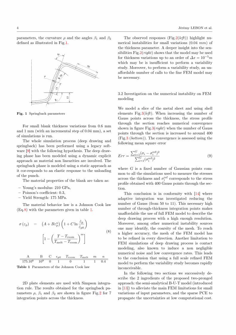
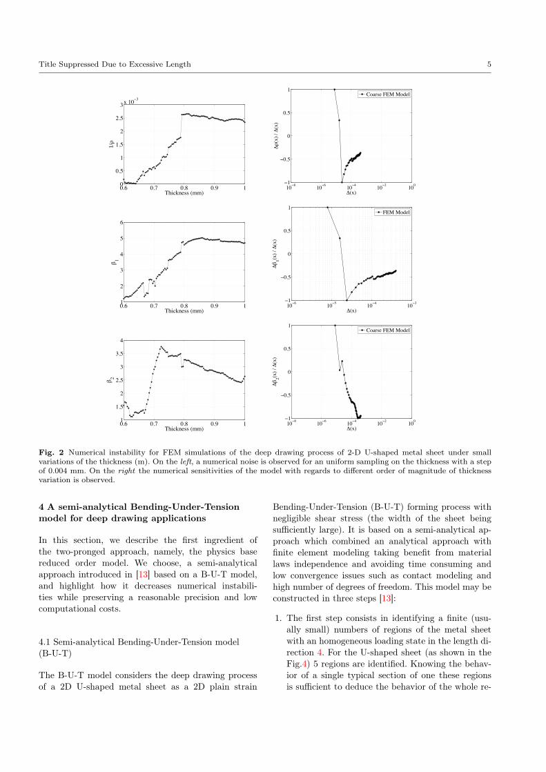
2D plate elements are used with Simpson integra-tion rule. The results obtained for the springback pa-rameters ρ, β1 and β2 are shown in figure Fig.2 for 7integration points across the thickness.

The observed responses (Fig.2(left)) highlight nu-merical instabilities for small variations (0.04 mm) ofthe thickness parameter. A deeper insight into the sen-sibilities Fig.2(right) shows that the model may be usedfor thickness variations up to an order of ∆x = 10−5m

which may be is insufficient to perform a variabilitystudy. Moreover, to perform a variability study, an un-affordable number of calls to the fine FEM model maybe necessary.

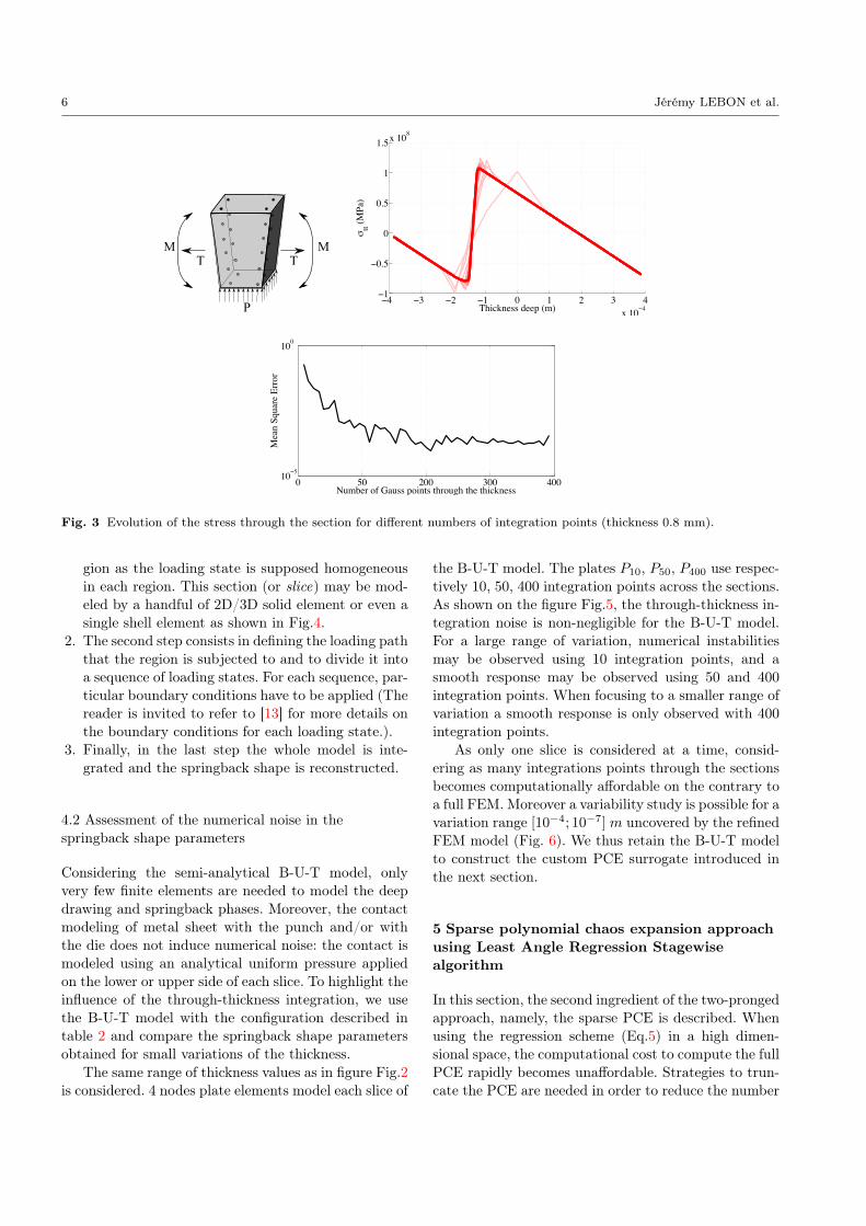
3.2 Investigation on the numerical instability on FEMmodeling

We model a slice of the metal sheet and using shellelements Fig.3(left). When increasing the number ofGauss points across the thickness, the stress profilethrough the section reaches numerical convergenceshown in figure Fig.3(right) when the number of Gausspoints through the section is increased to around 400(Fig.3 (bottom)). The convergence is assessed using thefollowing mean square error

Err =

∑Gi=1(σi − σref

i )2∑Gi=1(σ

refi )2

(9)

where G is a fixed number of Gaussian points com-mon to all the simulations used to measure the stressesacross the thickness and σref

i corresponds to the stressprofile obtained with 400 Gauss points through the sec-tion.

This conclusion is in conformity with [14] whereadaptive integration was investigated reducing thenumber of Gauss (from 50 to 11). This necessary highnumber of through-thickness integration points makesunaffordable the use of full FEM model to describe thedeep drawing process with a high enough resolution.Moreover, among other numerical instability sourcesone may identify, the coarsity of the mesh. To reacha higher accuracy, the mesh of the FEM model hasto be refined in every direction. Another limitation toFEM simulations of deep drawing process is contactmodeling, also known to induce a non negligiblenumerical noise and low convergence rates. This leadsto the conclusion that using a full scale refined FEMmodel to perform the variability study becomes rapidlyinconceivable.

In the following two sections we successively de-scribe the 2 ingredients of the proposed two-prongedapproach: the semi-analytical B-U-T model (introducedin [13]) to alleviate the main FEM limitations for smallvariations of input parameters, and the sparse PCE topropagate the uncertainties at low computational cost.

Title Suppressed Due to Excessive Length 5

0.6 0.7 0.8 0.9 10

0.5

1

1.5

2

2.5

3x 10 3

Thickness (mm)

1/

10 8 10 6 10 4 10 2 1001

0.5

0

0.5

1

(x)

(x) /

(x

)

Coarse FEM Model

0.6 0.7 0.8 0.9 11

2

3

4

5

6

Thickness (mm)

1

10 6 10 5 10 4 10 31

0.5

0

0.5

1

(x)

1(x) /

(x

)

FEM Model

0.6 0.7 0.8 0.9 11

1.5

2

2.5

3

3.5

4

Thickness (mm)

2

10 8 10 6 10 4 10 2 1001

0.5

0

0.5

1

(x)

2(x) /

(x

)

Coarse FEM Model

Fig. 2 Numerical instability for FEM simulations of the deep drawing process of 2-D U-shaped metal sheet under smallvariations of the thickness (m). On the left, a numerical noise is observed for an uniform sampling on the thickness with a stepof 0.004 mm. On the right the numerical sensitivities of the model with regards to different order of magnitude of thicknessvariation is observed.

4 A semi-analytical Bending-Under-Tensionmodel for deep drawing applications

In this section, we describe the first ingredient ofthe two-pronged approach, namely, the physics basereduced order model. We choose, a semi-analyticalapproach introduced in [13] based on a B-U-T model,and highlight how it decreases numerical instabili-ties while preserving a reasonable precision and lowcomputational costs.

4.1 Semi-analytical Bending-Under-Tension model(B-U-T)

The B-U-T model considers the deep drawing processof a 2D U-shaped metal sheet as a 2D plain strain

Bending-Under-Tension (B-U-T) forming process withnegligible shear stress (the width of the sheet beingsufficiently large). It is based on a semi-analytical ap-proach which combined an analytical approach withfinite element modeling taking benefit from materiallaws independence and avoiding time consuming andlow convergence issues such as contact modeling andhigh number of degrees of freedom. This model may beconstructed in three steps [13]:

1. The first step consists in identifying a finite (usu-ally small) numbers of regions of the metal sheetwith an homogeneous loading state in the length di-rection 4. For the U-shaped sheet (as shown in theFig.4) 5 regions are identified. Knowing the behav-ior of a single typical section of one these regionsis sufficient to deduce the behavior of the whole re-

6 Jérémy LEBON et al.

T TM M

P4 3 2 1 0 1 2 3 4

x 10 4

1

0.5

0

0.5

1

1.5x 108

Thickness deep (m)

tt (MPa

)

0 50 200 300 40010 5

100

Number of Gauss points through the thickness

Mea

n Sq

uare

Err

or

Fig. 3 Evolution of the stress through the section for different numbers of integration points (thickness 0.8 mm).

gion as the loading state is supposed homogeneousin each region. This section (or slice) may be mod-eled by a handful of 2D/3D solid element or even asingle shell element as shown in Fig.4.

2. The second step consists in defining the loading paththat the region is subjected to and to divide it intoa sequence of loading states. For each sequence, par-ticular boundary conditions have to be applied (Thereader is invited to refer to [13] for more details onthe boundary conditions for each loading state.).

3. Finally, in the last step the whole model is inte-grated and the springback shape is reconstructed.

4.2 Assessment of the numerical noise in thespringback shape parameters

Considering the semi-analytical B-U-T model, onlyvery few finite elements are needed to model the deepdrawing and springback phases. Moreover, the contactmodeling of metal sheet with the punch and/or withthe die does not induce numerical noise: the contact ismodeled using an analytical uniform pressure appliedon the lower or upper side of each slice. To highlight theinfluence of the through-thickness integration, we usethe B-U-T model with the configuration described intable 2 and compare the springback shape parametersobtained for small variations of the thickness.

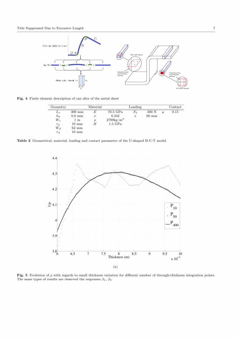
The same range of thickness values as in figure Fig.2is considered. 4 nodes plate elements model each slice of

the B-U-T model. The plates P10, P50, P400 use respec-tively 10, 50, 400 integration points across the sections.As shown on the figure Fig.5, the through-thickness in-tegration noise is non-negligible for the B-U-T model.For a large range of variation, numerical instabilitiesmay be observed using 10 integration points, and asmooth response may be observed using 50 and 400integration points. When focusing to a smaller range ofvariation a smooth response is only observed with 400integration points.

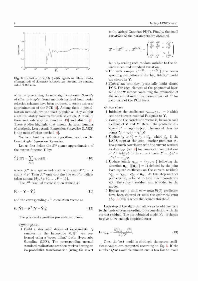
As only one slice is considered at a time, consid-ering as many integrations points through the sectionsbecomes computationally affordable on the contrary toa full FEM. Moreover a variability study is possible for avariation range [10−4; 10−7] m uncovered by the refinedFEM model (Fig. 6). We thus retain the B-U-T modelto construct the custom PCE surrogate introduced inthe next section.

5 Sparse polynomial chaos expansion approachusing Least Angle Regression Stagewisealgorithm

In this section, the second ingredient of the two-prongedapproach, namely, the sparse PCE is described. Whenusing the regression scheme (Eq.5) in a high dimen-sional space, the computational cost to compute the fullPCE rapidly becomes unaffordable. Strategies to trun-cate the PCE are needed in order to reduce the number

Title Suppressed Due to Excessive Length 7

+ + + +

l0

h05!

Fig. 4 Finite element description of one slice of the metal sheet

Geometry Material Loading ContactLs 300 mm E 70.5 GPa Fb 300 N µ 0.15h0 0.8 mm ν 0.342 s 60 mmWs 1 m ρ 2700kg/m3

rp 10 mm H 1.5 GPaWd 62 mmrd 10 mm

Table 2 Geometrical, material, loading and contact parameter of the U-shaped B-U-T model

6 6.5 7 7.5 8 8.5 9 9.5 10x 10 4

3.8

3.9

4

4.1

4.2

4.3

4.4

Thickness (m)

1/

P10

P50

P400

(a)

Fig. 5 Evolution of ρ with regards to small thickness variation for different number of through-thickness integration points.The same types of results are observed the responses β1, β2.

8 Jérémy LEBON et al.

10 10 10 9 10 8 10 7 10 6 10 5 10 40.2

0.15

0.1

0.05

0

(x)

(x) /

(x

)

Fig. 6 Evolution of ∆ρ/∆(x) with regards to different orderof magnitude of thickness variation ∆x, around the nominalvalue of 0.8 mm.

of terms by retaining the most significant ones (Sparsityof effect principle). Some methods inspired from modelselection schemes have been proposed to create a sparseapproximation of the PCE [2]. Among them l1 penal-ization methods are the most popular as they exhibita natural ability towards variable selection. A revue ofthese methods may be found in [19] and also in [8].These studies highlight that among the great numberof methods, Least Angle Regression Stagewise (LARS)is the most efficient method [6].

We here build a custom algorithm based on theLeast Angle Regression Stagewise.

Let us first define the J th-sparse approximation ofthe output function Y by:

Y JA (Ξ) =∑j∈A

γjψj(Ξ) (10)

where A∗∗ is a sparse index set with card(A∗∗) = J

and J ≤ P . Then A∗∗ only contains the set of J indicestaken among {Ψj , j ∈ {0, . . . , P − 1}}.

The J th residual vector is then defined as:

RJ = Y − YJA (11)

and the corresponding J th correlation vector as

cJ(Y) = Ψ>(Y − YJA) (12)

The proposed algorithm proceeds as follows:

Offline phase:1 Build a stochastic design of experiments. Q

samples on the hypercube [0, 1]M are per-formed using a “space filling” Latin HypercubeSampling (LHS). The corresponding normalstandard realizations are then retrieved using aniso-probabilist transformation (using the invert

multi-variate Gaussian PDF). Finally, the smallvariations of the parameters are obtained.

Ξ = {Ξ(1), . . . ,Ξ(M)} =

ξ(1)1 ξ

(1)2 ... ξ

(1)M

ξ(2)1 ξ

(2)2 ... ξ

(2)M

......

. . ....

ξ(Q)1 ξ

(Q)2 ... ξ

(Q)M

built by scaling each random variable to the de-sired mean and standard variation.

2 For each sample {Ξ(1), . . . ,Ξ(M)} the corre-sponding evaluations of the “high fidelity” modelare stored in Y.

3 Choose an arbitrary (eventually high) degreePCE. For each element of the polynomial basisbuild the Ψ matrix containing the evaluation ofthe normal standardized counterpart of Ξ foreach term of the PCE basis.

Online phase1 Initialize the coefficients γ0, ..., γP−1 = 0 whichsets the current residual R equals to Y.

2 Compute the correlation vector c0 between eachelement of Ψ and Y. Retain the predictor ψj∗where j∗ = argmax|c0|. The model then be-comes Y = γjψj = γ

>(1)ψ.

3 Update γj to γ∗j = γj + ε∗(1), where ε∗(1) is the

LARS step: at this step, another predictor ψl∗has as much correlation with the current residualas does ψj∗ (see [6] for numerical computationsof ε∗). Add ψ∗l to the current basis: Y = γ∗jψ

∗+

γ∗l ψ∗l = γ>(2)ψ.

4 Update jointly γ(2) = {γj∗ , γl∗} following thedirection u(2) (‖u(2)‖ = 1) defined by the jointleast-square coefficient on the current residual:γ∗(2) = γ(2) + ε

∗(2) × u(2). At this step another

predictor ψk is found to have much correlationwith the current residual and is added to themodel.

5 Repeat step 4 until m = min(P ;Q) predictorshave been entered or until the empirical error(Eq.13) has reached the desired threshold.

Each step of the algorithm allows us to add one termto the basis chosen according to its correlation with thecurrent residual. The best obtained model YA∗ is chosento give a low enough empirical error

Erremp =E[(fA − f)2]

σ(f)2. (13)

Once the best model is obtained, the sparse coeffi-cients values are computed according to Eq. 5. If thenumber Q of available simulations is too low to reach

Title Suppressed Due to Excessive Length 9

the condition Q ≥ 2− 3× P then the design of experi-ment may be enriched and the previous algorithm ranagain. As all computations are analytical, running thealgorithm as many times as necessary is considered tohave a negligible cost.

The combination of LARS and PCE allows us topropagate the uncertainties through the model at lowcomputational costs. Nevertheless the accuracy of theresults highly depends on the accuracy of the “high fi-delity” model which has to be accurate for small randomvariations on the input parameters.

6 Illustration of the two-pronged B-U-T/SparsePCE approach

In this section, we combine the ingredients of the two-pronged approach on the springback variability assess-ment of a 2D deep drawn U-shaped metal sheet in-troduced in section 3.1. We demonstrate the validityof the proposed approach firstly when a single randomvariable (blank initial thickness) is considered (mono-variate case) and then the whole probabilistic model isconsidered (multi-variate case) in which the standardvariation has been arbitrarily fixed at 3% of the meanvalue for each variable so that the variation of each vari-able implies a variation in the input parameters with acomparable order of magnitude.

Parameters Mean Std devBlank thickness ML2 0.8 mm 3%Young’s modulus ME0 7.05e10 Pa 3%Yield Strength MSy0 1.80e8 Pa 3%

Poisson’s coefficients MNu0 0.342 3%Friction coefficients PAFrot0 1.50e-1 3%Radius of the punch OR0 1.00e-2 mm 3%Radius of the matrix MR0 1.00e-2 mm 3%

Clamp force PForc0 3.00e-1 N 3%

Table 3 Stochastic input normal random variables for thespringback shape parameters study

6.1 Mono-variate case using Full PCE

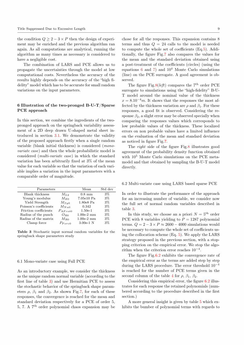
As an introductory example, we consider the thicknessas the unique random normal variable (according to thefirst line of table 3) and use Hermitian PCE to assessthe stochastic behavior of the springback shape param-eters ρ, β1 and β2. As shown Fig.7, for each of theseresponses, the convergence is reached for the mean andstandard deviation respectively for a PCE of order 5,5, 7. A 7th order polynomial chaos expansion may be

chose for all the responses. This expansion contains 8terms and thus Q = 24 calls to the model is neededto compute the whole set of coefficients (Eq.5). Addi-tionally, the figure Fig.7 also compares the values forthe mean and the standard deviation obtained usinga post-treatment of the coefficients (circles) (using theequations 6 and 7) and 104 Monte Carlo simulations(line) on the PCE surrogate. A good agreement is ob-served.

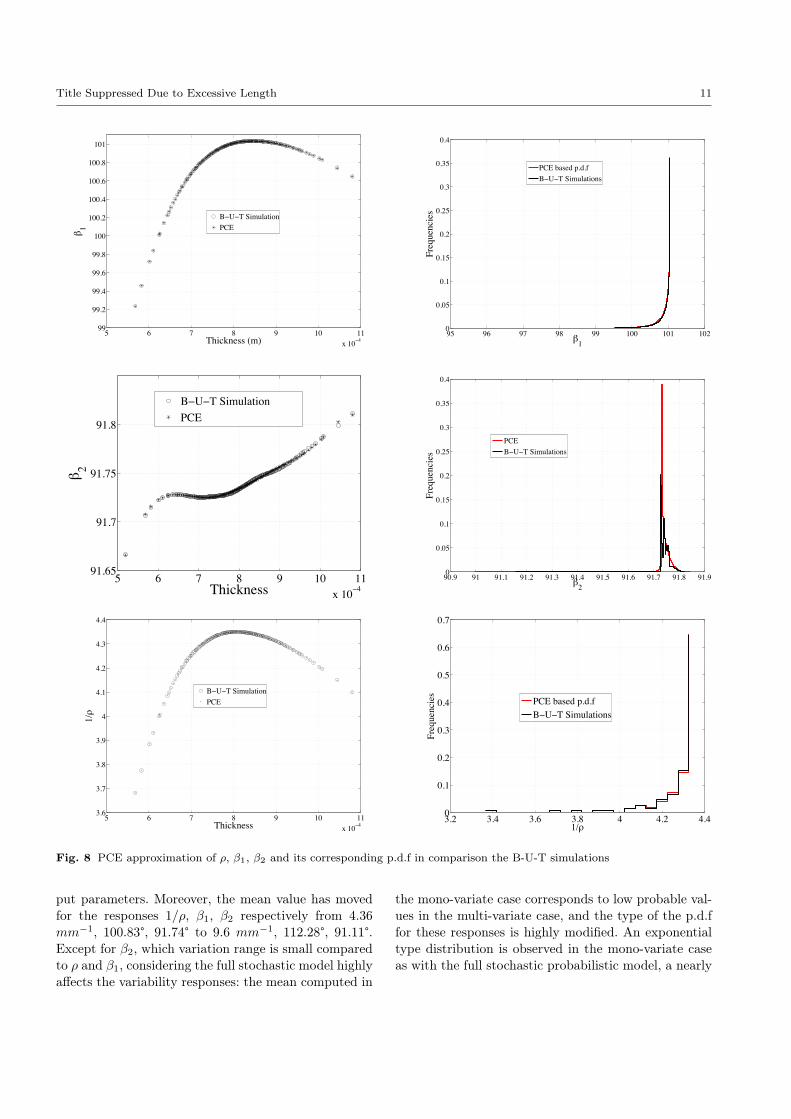
The figure Fig.8(left) compares the 7th order PCEsurrogate to simulations using the “high-fidelity” B-U-T model around the nominal value of the thicknessx = 8.10−4m. It shows that the responses the most af-fected by the thickness variation are ρ and β1. For theseresponses, a good fit is observed. Considering the re-sponse β2, a slight error may be observed specially whencomparing the responses values which corresponds tolow probable values of the thickness. These localizederrors on non probable values have a limited influenceon the evaluation of the mean and standard deviationas noticed in figure Fig.7.

The right side of the figure Fig.8 illustrates goodagreement of the probability density function obtainedwith 105 Monte Carlo simulations on the PCE meta-model and that obtained by sampling the B-U-T modeldirectly.

6.2 Multi-variate case using LARS based sparse PCE

In order to illustrate the performance of the approachfor an increasing number of variable, we consider nowthe full set of normal random variables described intable 3.

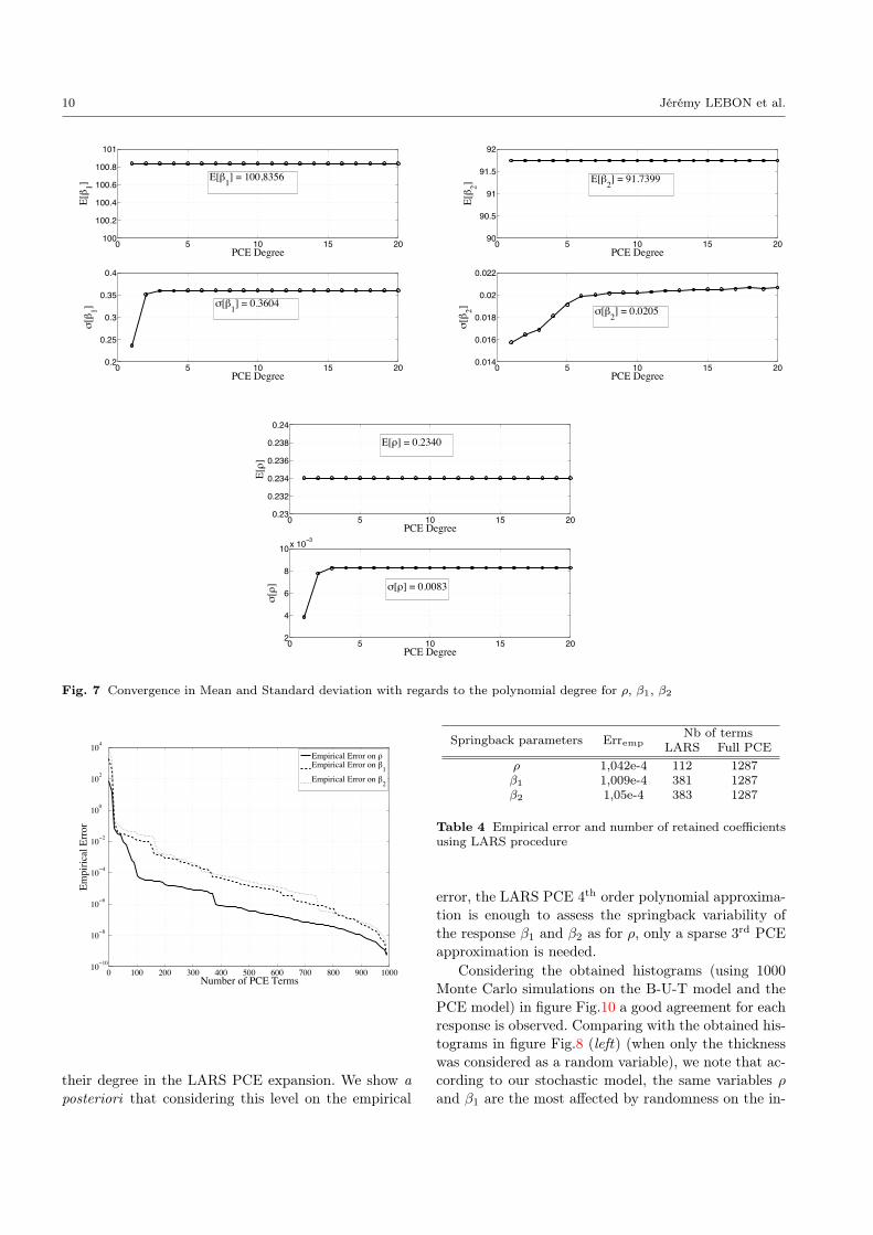
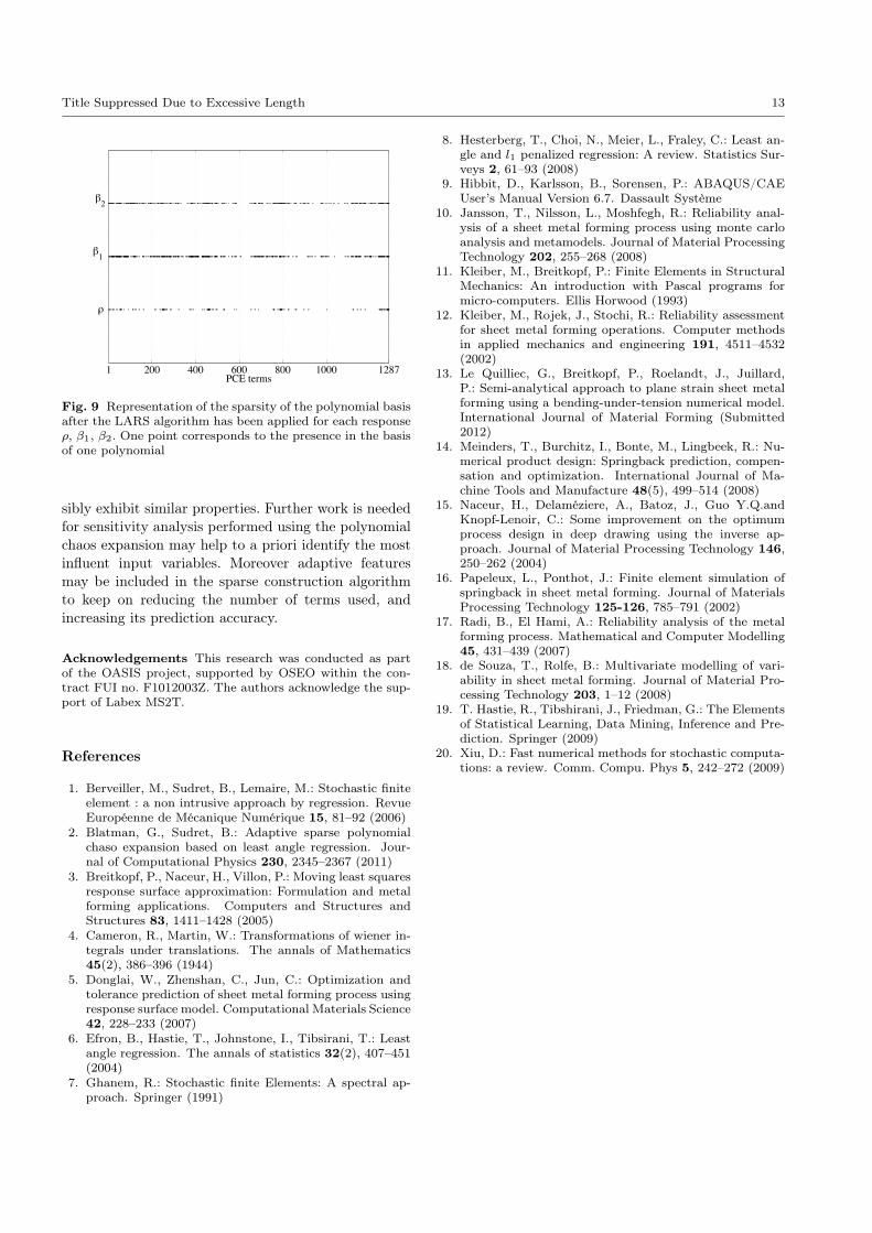
In this study, we choose an a priori N = 5th orderPCE with 8 variables yielding to P = 1287 polynomialterms. Q = 2− 3×P ≈ 2600− 4000 simulations wouldbe necessary to compute the whole set of coefficients us-ing the collocation scheme (Eq. 5). We apply the LARSstrategy proposed in the previous section, with a stop-ping criterion on the empirical error. We stop the algo-rithm when the criterion error reaches 10−4.

The figure Fig.6.2 exhibits the convergence rate ofthe empirical error as the terms are added step by stepduring the LARS procedure. The error threshold 10−4

is reached for the number of PCE terms given in thesecond column of the table 4 for ρ, β1, β2.

Considering this empirical error, the figure 6.2 illus-trates for each response the retained polynomials (num-bered according to the procedure described in the firstsection.)

A more general insight is given by table 5 which ex-hibits the bumber of polynomial terms with regards to

10 Jérémy LEBON et al.

0 5 10 15 20100

100.2

100.4

100.6

100.8

101

E[1]

PCE Degree

0 5 10 15 200.2

0.25

0.3

0.35

0.4

[1]

PCE Degree

E[ 1] = 100,8356

[ 1] = 0.3604

0 5 10 15 2090

90.5

91

91.5

92

E[2]

PCE Degree

0 5 10 15 200.014

0.016

0.018

0.02

0.022

[2]

PCE Degree

E[ 2] = 91.7399

[ 2] = 0.0205

0 5 10 15 200.23

0.232

0.234

0.236

0.238

0.24

E[]

PCE Degree

0 5 10 15 202

4

6

8

10x 10 3

[]

PCE Degree

E[ ] = 0.2340

[ ] = 0.0083

Fig. 7 Convergence in Mean and Standard deviation with regards to the polynomial degree for ρ, β1, β2

0 100 200 300 400 500 600 700 800 900 100010 10

10 8

10 6

10 4

10 2

100

102

104

Number of PCE Terms

Empi

rical

Err

or

Empirical Error on Empirical Error on 1Empirical Error on 2

their degree in the LARS PCE expansion. We show aposteriori that considering this level on the empirical

Springback parameters ErrempNb of terms

LARS Full PCEρ 1,042e-4 112 1287β1 1,009e-4 381 1287β2 1,05e-4 383 1287

Table 4 Empirical error and number of retained coefficientsusing LARS procedure

error, the LARS PCE 4th order polynomial approxima-tion is enough to assess the springback variability ofthe response β1 and β2 as for ρ, only a sparse 3rd PCEapproximation is needed.

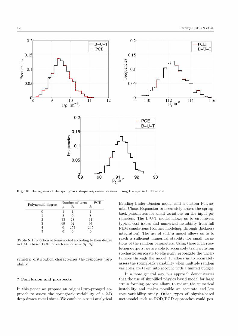
Considering the obtained histograms (using 1000Monte Carlo simulations on the B-U-T model and thePCE model) in figure Fig.10 a good agreement for eachresponse is observed. Comparing with the obtained his-tograms in figure Fig.8 (left) (when only the thicknesswas considered as a random variable), we note that ac-cording to our stochastic model, the same variables ρand β1 are the most affected by randomness on the in-

Title Suppressed Due to Excessive Length 11

5 6 7 8 9 10 11x 10 4

99

99.2

99.4

99.6

99.8

100

100.2

100.4

100.6

100.8

101

Thickness (m)

1

B U T SimulationPCE

95 96 97 98 99 100 101 1020

0.05

0.1

0.15

0.2

0.25

0.3

0.35

0.4

1

Freq

uenc

ies

PCE based p.d.fB U T Simulations

5 6 7 8 9 10 11x 10 4

91.65

91.7

91.75

91.8

Thickness

2

B U T SimulationPCE

90.9 91 91.1 91.2 91.3 91.4 91.5 91.6 91.7 91.8 91.90

0.05

0.1

0.15

0.2

0.25

0.3

0.35

0.4

2

Freq

uenc

ies

PCE B U T Simulations

5 6 7 8 9 10 11x 10 4

3.6

3.7

3.8

3.9

4

4.1

4.2

4.3

4.4

Thickness

1/

B U T SimulationPCE

3.2 3.4 3.6 3.8 4 4.2 4.40

0.1

0.2

0.3

0.4

0.5

0.6

0.7

1/

Freq

uenc

ies

PCE based p.d.fB U T Simulations

Fig. 8 PCE approximation of ρ, β1, β2 and its corresponding p.d.f in comparison the B-U-T simulations

put parameters. Moreover, the mean value has movedfor the responses 1/ρ, β1, β2 respectively from 4.36mm−1, 100.83°, 91.74° to 9.6 mm−1, 112.28°, 91.11°.Except for β2, which variation range is small comparedto ρ and β1, considering the full stochastic model highlyaffects the variability responses: the mean computed in

the mono-variate case corresponds to low probable val-ues in the multi-variate case, and the type of the p.d.ffor these responses is highly modified. An exponentialtype distribution is observed in the mono-variate caseas with the full stochastic probabilistic model, a nearly

12 Jérémy LEBON et al.

8 9 10 11 120

0.05

0.1

0.15

0.2

1/ (m 1)

Freq

uenc

ies

B U T PCE

110 112 114 1160

0.05

0.1

0.15

0.2

1 in o

Freq

uenc

ies

PCEB U T

89 90 91 92 930

0.05

0.1

0.15

0.2

2 in o

Freq

uenc

ies

PCEB U T

Fig. 10 Histograms of the springback shape responses obtained using the sparse PCE model

Polynomial degree Number of terms in PCEρ β1 β2

0 1 1 11 8 6 82 33 28 313 69 92 974 0 254 2455 0 0 0

Table 5 Proportion of terms sorted according to their degreein LARS based PCE for each response ρ, β1, β2

symetric distribution characterizes the responses vari-ability.

7 Conclusion and prospects

In this paper we propose an original two-pronged ap-proach to assess the springback variability of a 2-Ddeep drawn metal sheet. We combine a semi-analytical

Bending-Under-Tension model and a custom Polyno-mial Chaos Expansion to accurately assess the spring-back parameters for small variations on the input pa-rameters. The B-U-T model allows us to circumventtypical cost issues and numerical instability from fullFEM simulations (contact modeling, through thicknessintegration). The use of such a model allows us to toreach a sufficient numerical stability for small varia-tions of the random parameters. Using these high reso-lution outputs, we are able to accurately train a customstochastic surrogate to efficiently propagate the uncer-tainties through the model. It allows us to accuratelyassess the springback variability when multiple randomvariables are taken into account with a limited budget.

In a more general way, our approach demonstratesthat the use of simplified physics based model for largestrain forming process allows to reduce the numericalinstability and makes possible an accurate and lowcost variability study. Other types of physics-basedmetamodel such as POD/PGD approaches could pos-

Title Suppressed Due to Excessive Length 13

1 200 400 600 800 1000 1287PCE terms

1

2

Fig. 9 Representation of the sparsity of the polynomial basisafter the LARS algorithm has been applied for each responseρ, β1, β2. One point corresponds to the presence in the basisof one polynomial

sibly exhibit similar properties. Further work is neededfor sensitivity analysis performed using the polynomialchaos expansion may help to a priori identify the mostinfluent input variables. Moreover adaptive featuresmay be included in the sparse construction algorithmto keep on reducing the number of terms used, andincreasing its prediction accuracy.

Acknowledgements This research was conducted as partof the OASIS project, supported by OSEO within the con-tract FUI no. F1012003Z. The authors acknowledge the sup-port of Labex MS2T.

References

1. Berveiller, M., Sudret, B., Lemaire, M.: Stochastic finiteelement : a non intrusive approach by regression. RevueEuropéenne de Mécanique Numérique 15, 81–92 (2006)

2. Blatman, G., Sudret, B.: Adaptive sparse polynomialchaso expansion based on least angle regression. Jour-nal of Computational Physics 230, 2345–2367 (2011)

3. Breitkopf, P., Naceur, H., Villon, P.: Moving least squaresresponse surface approximation: Formulation and metalforming applications. Computers and Structures andStructures 83, 1411–1428 (2005)

4. Cameron, R., Martin, W.: Transformations of wiener in-tegrals under translations. The annals of Mathematics45(2), 386–396 (1944)

5. Donglai, W., Zhenshan, C., Jun, C.: Optimization andtolerance prediction of sheet metal forming process usingresponse surface model. Computational Materials Science42, 228–233 (2007)

6. Efron, B., Hastie, T., Johnstone, I., Tibsirani, T.: Leastangle regression. The annals of statistics 32(2), 407–451(2004)

7. Ghanem, R.: Stochastic finite Elements: A spectral ap-proach. Springer (1991)

8. Hesterberg, T., Choi, N., Meier, L., Fraley, C.: Least an-gle and l1 penalized regression: A review. Statistics Sur-veys 2, 61–93 (2008)

9. Hibbit, D., Karlsson, B., Sorensen, P.: ABAQUS/CAEUser’s Manual Version 6.7. Dassault Système

10. Jansson, T., Nilsson, L., Moshfegh, R.: Reliability anal-ysis of a sheet metal forming process using monte carloanalysis and metamodels. Journal of Material ProcessingTechnology 202, 255–268 (2008)

11. Kleiber, M., Breitkopf, P.: Finite Elements in StructuralMechanics: An introduction with Pascal programs formicro-computers. Ellis Horwood (1993)

12. Kleiber, M., Rojek, J., Stochi, R.: Reliability assessmentfor sheet metal forming operations. Computer methodsin applied mechanics and engineering 191, 4511–4532(2002)

13. Le Quilliec, G., Breitkopf, P., Roelandt, J., Juillard,P.: Semi-analytical approach to plane strain sheet metalforming using a bending-under-tension numerical model.International Journal of Material Forming (Submitted2012)

14. Meinders, T., Burchitz, I., Bonte, M., Lingbeek, R.: Nu-merical product design: Springback prediction, compen-sation and optimization. International Journal of Ma-chine Tools and Manufacture 48(5), 499–514 (2008)

15. Naceur, H., Delaméziere, A., Batoz, J., Guo Y.Q.andKnopf-Lenoir, C.: Some improvement on the optimumprocess design in deep drawing using the inverse ap-proach. Journal of Material Processing Technology 146,250–262 (2004)

16. Papeleux, L., Ponthot, J.: Finite element simulation ofspringback in sheet metal forming. Journal of MaterialsProcessing Technology 125-126, 785–791 (2002)

17. Radi, B., El Hami, A.: Reliability analysis of the metalforming process. Mathematical and Computer Modelling45, 431–439 (2007)

18. de Souza, T., Rolfe, B.: Multivariate modelling of vari-ability in sheet metal forming. Journal of Material Pro-cessing Technology 203, 1–12 (2008)

19. T. Hastie, R., Tibshirani, J., Friedman, G.: The Elementsof Statistical Learning, Data Mining, Inference and Pre-diction. Springer (2009)

20. Xiu, D.: Fast numerical methods for stochastic computa-tions: a review. Comm. Compu. Phys 5, 242–272 (2009)