A two-objective evolutionary approach based on topological constraints for node localization in...

A

Al

Ma

b

a

ARRAA

KWNRSM

1

otegdllodtctM

Da

v

1d

ARTICLE IN PRESSG ModelSOC-1144; No. of Pages 11

Applied Soft Computing xxx (2011) xxx–xxx

Contents lists available at ScienceDirect

Applied Soft Computing

journa l homepage: www.e lsev ier .com/ locate /asoc

two-objective evolutionary approach based on topological constraints for nodeocalization in wireless sensor networks�

assimo Vecchioa,∗, Roberto López-Valcarcea, Francesco Marcellonib

Departamento de Teoría de la Senal y las Comunicaciones, University of Vigo, C/ Maxwell s/n, 36310 Vigo, SpainDipartimento di Ingegneria dell’Informazione, University of Pisa, Via Diotisalvi 2, 56122 Pisa, Italy

r t i c l e i n f o

rticle history:eceived 1 October 2010eceived in revised form 23 February 2011ccepted 16 March 2011vailable online xxx

eywords:ireless sensor networks

ode localization

a b s t r a c t

To know the location of nodes plays an important role in many current and envisioned wireless sensornetwork applications. In this framework, we consider the problem of estimating the locations of allthe nodes of a network, based on noisy distance measurements for those pairs of nodes in range ofeach other, and on a small fraction of anchor nodes whose actual positions are known a priori. Themethods proposed so far in the literature for tackling this non-convex problem do not generally provideaccurate estimates. The difficulty of the localization task is exacerbated by the fact that the networkis not generally uniquely localizable when its connectivity is not sufficiently high. In order to alleviatethis drawback, we propose a two-objective evolutionary algorithm which takes concurrently into account

ange measurementstochastic optimizationultiobjective evolutionary algorithms

during the evolutionary process both the localization accuracy and certain topological constraints inducedby connectivity considerations. The proposed method is tested with different network configurationsand sensor setups, and compared in terms of normalized localization error with another metaheuristicapproach, namely SAL, based on simulated annealing. The results show that, in all the experiments,our approach achieves considerable accuracies and significantly outperforms SAL, thus manifesting itseffectiveness and stability.

© 2011 Elsevier B.V. All rights reserved.

. Introduction

A wireless sensor network (WSN) may consist of hundredsr even thousands of low-cost nodes communicating amonghemselves [1]. Among classical applications of WSNs, one findsnvironmental and structural monitoring, event detection, tar-et tracking, etc. In many of these applications, tiny nodes areeployed in an area to be monitored, thus spanning a potentially

arge geographical region. Each node is a small device that col-ects information from the surrounding environment through oner more sensors, processes this information locally, and exchangesata through a wireless channel. The small size and low cost ofhe nodes impose several physical limitations; in particular, they

Please cite this article in press as: M. Vecchio, et al., A two-objective elocalization in wireless sensor networks, Appl. Soft Comput. J. (2011),

annot mount powerful microprocessors or large memory devices,hus computational and storage capabilities are tightly constrained.

oreover, they are typically powered by small batteries which in

� This work was supported by the Spanish Government and the European Regionalevelopment Fund (ERDF), under projects DYNACS (TEC2010-21245-C02-02/TCM),nd COMONSENS (CONSOLIDER-INGENIO 2010 CSD2008-00010).∗ Corresponding author. Tel.: +34 986 818659; fax: +34 986 812116.

E-mail addresses: [email protected] (M. Vecchio),[email protected] (R. López-Valcarce), [email protected] (F. Marcelloni).

568-4946/$ – see front matter © 2011 Elsevier B.V. All rights reserved.oi:10.1016/j.asoc.2011.03.012

general cannot be easily changed or recharged. A consequence ofthese limitations is the need to save energy in order to extend thenetwork lifetime [2,3].

In many envisioned or existent applications, such as envi-ronment monitoring, precision agriculture, vehicle tracking, andlogistics, knowledge about the location of sensor nodes plays akey role. In addition, location-based routing protocols can save sig-nificant energy by eliminating the need for route discovery, andimprove caching behavior for applications where requests maybe location-dependent. Finally, security can also be enhanced bylocation awareness (see [4] and the references therein). Althoughlocation awareness can be enabled in principle by the use of aGlobal Positioning System (GPS), this solution is not always viablein practice, as the cost and power consumption of GPS receiversare not negligible. In addition, GPS is not well suited to indoor andunderground deployments, and the presence of obstacles like densefoliage or tall buildings may impair the outdoor communicationwith satellites.

These limitations have motivated alternative approaches to theproblem, as reviewed in [5–7], among which fine-grained localiza-

volutionary approach based on topological constraints for nodedoi:10.1016/j.asoc.2011.03.012

tion techniques may represent the most suitable ones. In theseschemes, only a few nodes of the network (the reference or anchornodes) are endowed with their exact positions through GPS ormanual placement, while all nodes are able to estimate their

dx.doi.org/10.1016/j.asoc.2011.03.012

dx.doi.org/10.1016/j.asoc.2011.03.012

http://www.sciencedirect.com/science/journal/15684946

www.elsevier.com/locate/asoc

mailto:[email protected]



dx.doi.org/10.1016/j.asoc.2011.03.012

ARTICLE IN PRESSG ModelASOC-1144; No. of Pages 11

2 M. Vecchio et al. / Applied Soft Computing xxx (2011) xxx–xxx

i

i'jk

l

m

n

dT(AinamtmmmTanf

(niafeclmiiatw

Ft

Fig. 1. The flip ambiguity problem.

istances to nearby nodes using any measurement technique.hese distance-related techniques include Received Signal StrengthRSS) measurements, Time of Arrival (ToA), Time Difference ofrrival (TDoA), etc. (for a review of these techniques the reader

s referred to [6,7]). Thus, assuming that the coordinates of anchorodes are known, and exploiting pairwise distance measurementsmong the nodes, the fine-grained localization problem is to deter-ine the positions of all non-anchor nodes. This task has proved

o be rather difficult, due to the following reasons. First, deter-ining the locations of the nodes from a set of pairwise distanceeasurements is a nonconvex optimization problem. Second, theeasurements available to nodes are invariably corrupted by noise.

hird, even if the distance measurements were perfectly accurate,sufficient condition for the topology to be uniquely localizable isot easily identified [8]. We will briefly discuss these issues in the

ollowing.Given a statistical characterization of measurement noise

which will depend on the kind of adopted measurement tech-ique [6]), the most natural path to the localization problem

s the Maximum-Likelihood (ML) estimation approach. As statedbove, this results in a multivariable nonconvex optimization task,or which three different approaches can be found in the lit-rature: stochastic optimization, multidimensional scaling, andonvex relaxation. The first class of techniques attempt to avoidocal maxima of the likelihood function via global optimization

ethods, such as simulated annealing [9]. Multidimensional scal-ng (MDS) [10,11] is a connectivity-based technique, i.e., it exploits

Please cite this article in press as: M. Vecchio, et al., A two-objectivelocalization in wireless sensor networks, Appl. Soft Comput. J. (2011),

nformation of “who is within range of whom” in the network, inddition to the distance measurements. This connectivity informa-ion imposes additional constraints on the problem, since nodesithin range of each other cannot be arbitrarily far apart. The third

ig. 2. Constraints imposed on class 2 nodes. (a) Node i is neighbor to node k, which in itsheir turns are neighbors to anchor nodes j and l, respectively.

Fig. 3. The chromosome coding.

class of methods relax the original ML formulation in order to obtaina Semi-Definite Programming (SDP) or a Second-Order Cone Pro-gramming (SOCP) problem. An approximate solution can be thenobtained in a globally optimum fashion with reduced computa-tional effort [8,12]. Since the relaxation may incur in non-negligibleestimation errors [13], additional refinements may be needed, forexample via gradient-descent iterations starting from the approx-imate solution [8].

The main advantage of SDP and SOCP is that the relaxation of theoriginal nonconvex problem reduces the computational load signif-icantly, making these methods well suited to large-scale and mobilenetwork localization problems; in these scenarios, the localizationalgorithm must trade off computation time for some accuracy in thefinal estimate. On the other hand, there are practical applicationsof WSNs which do not demand such highly scalable or real-timesolutions. Consider, for instance, a precision agriculture applica-tion: clearly, it is preferable to spend some additional time in orderto obtain an accurate estimate of the node coordinates, rather thane.g. administer a fertilizer to a wrong zone of the monitored field.Moreover, current existent sensor network testbeds are rarely com-posed by more than one hundred nodes and their mobility is mainlyenabled for security and surveillance applications. Motivated bythese considerations, we focus on developing localization schemesyielding accurate estimates, having in mind that they may not bewell suited to other applications that demand high scalability orrequire real-time operation. We advocate the use of a stochas-tic optimization technique, namely Multi-Objective EvolutionaryAlgorithms (MOEA), in order to solve the original nonconvex prob-lem.

In particular, we propose a two-objective evolutionary algo-rithm in which the first objective function, referred to as CF, isgiven by the original nonconvex cost (the squared error betweenthe estimated and the corresponding measured inter-node dis-tances). The second objective function, referred to as CV, is definedas the sum of neighborhood violations in the candidate topology.This second objective function exploits the connectivity-based apriori information about the network, and is especially useful inorder to alleviate localizability issues. Given a set of data comprisedby the set of anchor nodes and the inter-node distance measure-

evolutionary approach based on topological constraints for nodedoi:10.1016/j.asoc.2011.03.012

ments, a network is said to be localizable if there is only one possiblegeometry compatible with the data. Localizability is a fundamentalproblem which can be studied within the framework of rigid graphtheory [14]. If the network is not localizable, then multiple global

turn is neighbor to anchor node j. (b) Node i is neighbor to nodes m and n, which in

dx.doi.org/10.1016/j.asoc.2011.03.012


M. Vecchio et al. / Applied Soft Computing xxx (2011) xxx–xxx 3

F licatiom

mcsate

sntidibmttrns

ieulitlsaitprTimmtthaiwoadtitp

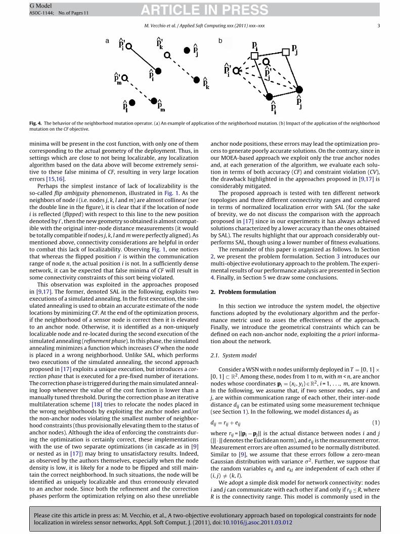
ig. 4. The behavior of the neighborhood mutation operator. (a) An example of apputation on the CF objective.

inima will be present in the cost function, with only one of themorresponding to the actual geometry of the deployment. Thus, inettings which are close to not being localizable, any localizationlgorithm based on the data above will become extremely sensi-ive to these false minima of CF, resulting in very large locationrrors [15,16].

Perhaps the simplest instance of lack of localizability is theo-called flip ambiguity phenomenon, illustrated in Fig. 1. As theeighbors of node i (i.e. nodes j, k, l and m) are almost collinear (seehe double line in the figure), it is clear that if the location of nodeis reflected (flipped) with respect to this line to the new positionenoted by i′, then the new geometry so obtained is almost compat-

ble with the original inter-node distance measurements (it woulde totally compatible if nodes j, k, l and m were perfectly aligned). Asentioned above, connectivity considerations are helpful in order

o combat this lack of localizability. Observing Fig. 1, one noticeshat whereas the flipped position i′ is within the communicationange of node n, the actual position i is not. In a sufficiently denseetwork, it can be expected that false minima of CF will result inome connectivity constraints of this sort being violated.

This observation was exploited in the approaches proposedn [9,17]. The former, denoted SAL in the following, exploits twoxecutions of a simulated annealing. In the first execution, the sim-lated annealing is used to obtain an accurate estimate of the node

ocations by minimizing CF. At the end of the optimization process,f the neighborhood of a sensor node is correct then it is elevatedo an anchor node. Otherwise, it is identified as a non-uniquelyocalizable node and re-located during the second execution of theimulated annealing (refinement phase). In this phase, the simulatednnealing minimizes a function which increases CF when the nodes placed in a wrong neighborhood. Unlike SAL, which performswo executions of the simulated annealing, the second approachroposed in [17] exploits a unique execution, but introduces a cor-ection phase that is executed for a pre-fixed number of iterations.he correction phase is triggered during the main simulated anneal-ng loop whenever the value of the cost function is lower than a

anually tuned threshold. During the correction phase an iterativeultilateration scheme [18] tries to relocate the nodes placed in

he wrong neighborhoods by exploiting the anchor nodes and/orhe non-anchor nodes violating the smallest number of neighbor-ood constraints (thus provisionally elevating them to the status ofnchor nodes). Although the idea of enforcing the constraints dur-ng the optimization is certainly correct, these implementations

ith the use of two separate optimizations (in cascade as in [9]r nested as in [17]) may bring to unsatisfactory results. Indeed,s observed by the authors themselves, especially when the nodeensity is low, it is likely for a node to be flipped and still main-


ain the correct neighborhood. In such situations, the node will bedentified as uniquely localizable and thus erroneously elevatedo an anchor node. Since both the refinement and the correctionhases perform the optimization relying on also these unreliable

n of the neighborhood mutation. (b) Impact of the application of the neighborhood

anchor node positions, these errors may lead the optimization pro-cess to generate poorly accurate solutions. On the contrary, since inour MOEA-based approach we exploit only the true anchor nodesand, at each generation of the algorithm, we evaluate each solu-tion in terms of both accuracy (CF) and constraint violation (CV),the drawback highlighted in the approaches proposed in [9,17] isconsiderably mitigated.

The proposed approach is tested with ten different networktopologies and three different connectivity ranges and comparedin terms of normalized localization error with SAL (for the sakeof brevity, we do not discuss the comparison with the approachproposed in [17] since in our experiments it has always achievedsolutions characterized by a lower accuracy than the ones obtainedby SAL). The results highlight that our approach considerably out-performs SAL, though using a lower number of fitness evaluations.

The remainder of this paper is organized as follows. In Section2, we present the problem formulation. Section 3 introduces ourmulti-objective evolutionary approach to the problem. The experi-mental results of our performance analysis are presented in Section4. Finally, in Section 5 we draw some conclusions.

2. Problem formulation

In this section we introduce the system model, the objectivefunctions adopted by the evolutionary algorithm and the perfor-mance metric used to asses the effectiveness of the approach.Finally, we introduce the geometrical constraints which can bedefined on each non-anchor node, exploiting the a priori informa-tion about the network.

2.1. System model

Consider a WSN with n nodes uniformly deployed in T = [0, 1] ×[0, 1] ⊂ R2. Among these, nodes from 1 to m, with m < n, are anchornodes whose coordinates pi = (xi, yi) ∈R2, i = 1, . . ., m, are known.In the following, we assume that, if two sensor nodes, say i andj, are within communication range of each other, their inter-nodedistance dij can be estimated using some measurement technique(see Section 1). In the following, we model distances dij as

dij = rij + eij (1)

where rij = ||pi − pj|| is the actual distance between nodes i and j(|| · || denotes the Euclidean norm), and eij is the measurement error.Measurement errors are often assumed to be normally distributed.Similar to [9], we assume that these errors follow a zero-meanGaussian distribution with variance �2. Further, we suppose thatthe random variables eij and ekl are independent of each other if


(i, j) /= (k, l).We adopt a simple disk model for network connectivity: nodes

i and j can communicate with each other if and only if rij ≤ R, whereR is the connectivity range. This model is commonly used in the

dx.doi.org/10.1016/j.asoc.2011.03.012



lshtrjln

N

N

br.d

Fig. 7. Average percentage of non-anchor nodes versus the number of anchor nodes

Fig. 5. The PAES algorithm.

iterature, although empirical measurements on real WSNs havehown that it is only an approximation in practice. On the otherand, different connectivity models could be adopted by modifyinghe geometrical analysis in Section 2.3. We refer to nodes j such thatij ≤ R as first-level neighbors of node i. Further, we refer to all nodeswhich are not first-level neighbors of node i, but which share at

east a first-level neighbor with node i, as second-level neighbors ofode i. Let

i = {j ∈ 1, . . . , n, j /= i : rij ≤ R} (2)

¯ i = {j ∈ 1, . . . , n, j /= i : rij > R} (3)

e the set of the first-level neighbors of node i and its complement,


espectively. We assume that sets Ni and Ni are known for all i = 1,. ., n. This is a reasonable assumption, since each node can easilyetermine which other nodes it can communicate with.

Fig. 6. Average percentage of nodes versus neighb

in their neighborhood for different values of R.

2.2. Objective functions and performance metric

Our goal is to estimate the positions of the non-anchor nodesas accurately as possible. Towards this goal, we aim to concur-rently minimize two objective functions. Let pi = (xi, yi), i = m +1, . . . , n be the estimated positions of the non-anchor nodes i. Thefirst objective CF is defined as:

CF =n∑

i=m+1

⎛⎝∑

j ∈ Ni

(dij − dij)2

⎞⎠ , (4)

where dij is the estimated distance between nodes i and j computedas follows:

dij =

⎧⎨⎩

√(xi − xj)

2 + (yi − yj)2 if node j is an anchor,√

(xi − xj)2 + (yi − yj)

2 otherwise.(5)

Thus, CF is the squared error between the inter-node distancescorresponding to the candidate geometry (as given by the esti-mated positions pi, i = m + 1, . . . , n of the non-anchor nodes and


the positions of the anchor nodes) and the measured data.The second objective function CV counts the number of connec-

tivity constraints which are not satisfied by the current estimated

orhood cardinality for different values of R.

dx.doi.org/10.1016/j.asoc.2011.03.012

IN PRESSG ModelA

ft Computing xxx (2011) xxx–xxx 5

p

C

w

t

N

2

dgwtbn

•

•

•

aipcitnctiptc

3

yMotNs

ARTICLESOC-1144; No. of Pages 11

M. Vecchio et al. / Applied So

ositions of non-anchor nodes. CV is defined as

V =n∑

i=m+1

⎛⎝∑

j ∈ Ni

ıij +∑j ∈ Ni

(1 − ıij)

⎞⎠ , (6)

here ıij = 1 if dij > R and 0 otherwise.The goodness of an estimate can be evaluated a posteriori using

he normalized localization error NLE defined as:

LE = 1R

√√√√ 1(n − m)

n∑i=m+1

((xi − xi)2 + (yi − yi)

2) × 100%. (7)

.3. Geometrical constraints

The connectivity ranges and the positions of the anchor nodesetermine subspaces of the overall search space where each sin-le non-anchor node can be positioned. These subspaces, whichill be expressed by means of geometrical constraints, depend on

he type of non-anchor node. We adopt the following classificationased on the position of a non-anchor node with respect to anchorodes:

Class 1 node: a non-anchor node which is first-level neighbor toat least one anchor node.

If a node belongs to Class 1, then its position must lie withinthe intersection of the circles of radius R centered in the anchornodes which it is neighbor to.Class 2 node: a non-anchor node which is second-level neighborto at least one anchor node.

If a node belongs to class 2, then its position must lie withinthe intersection of the annuli with inner and outer radii Rand 2R, respectively, centered in the anchor nodes which it issecond-level neighbor to. Fig. 2 shows two examples of class 2nodes.Class 3 node: a non-anchor node which belongs to neither class 1nor class 2.

If a node is class 3, then its position must lie outside the unionof the circles of radius R centered in all anchor nodes.

The membership of a non-anchor node to one of the three classesllows restricting the space where the node can be located. Thisnformation can be exploited both in the generation of the initialopulation of the MOEA and, during the evolutionary process, toonstrain the application of the mating operators. Thus, by avoid-ng generating solutions which certainly cannot be optimal (sincehey violate the geometrical constraints determined by the con-ectivity ranges and by the known anchor node positions), wean speed up the execution of the evolutionary algorithm. Further,hese constraints help alleviate the localizability issues discussedn Section 1 and in particular the flip ambiguity phenomenon. Thishenomenon is much more likely to occur if the candidate posi-ions of non-anchor nodes are not constrained within the subspaceorresponding to its membership class.

. The optimization framework

MOEAs have been investigated by several authors in recentears [19,20]. Although there exist a number of recently proposedOEAs with different peculiarities, we have focused our attention


n some of the most popular, namely the Strength Pareto Evolu-ionary Algorithm (SPEA) [21] and its evolution (SPEA2) [22], theiched Pareto Genetic Algorithm (NPGA) [23], the different ver-

ions of the Pareto Archived Evolution Strategy (PAES) [24], and

Fig. 8. Average distribution of the non-anchor nodes in the three classes introducedin Section 2.3. (a) R = 0.13; (b) R = 0.15; (c) R = 0.17.

the Non-dominated Sorting Genetic Algorithm (NSGA) [25] and itsevolution (NSGA-II) [26]. On the other hand, the main aim of thispaper is to demonstrate that the localization problem in wirelesssensor networks can be successfully tackled by an MOEA. Thus,we did not investigate whether recent MOEAs might improve theperformance, but simply used well-known algorithms. Besides,these algorithms are often used as benchmarks when proposingnew MOEAs. After some experimentation, we realized that PAESguaranteed fast convergence towards remarkable Pareto fronts.Further, the PAES evolutionary scheme is very similar to the sim-ulated annealing process exploited by SAL in [9], thus making thecomparison quite fair. Indeed, both PAES and SAL exploit a (1 + 1)optimization scheme: a single random initial solution is generatedand mutated (in PAES), or perturbed (in the simulated annealing), inorder to obtain a single solution. The key difference between themrelies on the generation of the mutated/perturbed solution: in PAESthe algorithm exploits the principles of the genetic evolution, whilethe simulated annealing resembles the temperature-lowering pro-cess used in metallurgy to ensure good quality of the final metalcast [27]. We have used the jMetal [28] implementation of PAES for


our optimization.In the following subsections, we describe the chromosome cod-

ing, the objective functions, the genetic operators and the PAESalgorithm.

dx.doi.org/10.1016/j.asoc.2011.03.012



70 80 90 100 110 120 130 1400.35

0.355

0.36

0.365

0.37

0.375

0.38

0.385

0.39

0.395

CF

3

pmeTrwem

wC

3

Wammgc

oedaitaspaps

uHsWitttibt

Table 1parameter setup of PAES.

Parameter Value

Archive size 20Number of regions 5Number of fitness evaluations 400,000

CV

Fig. 9. Final front of non-dominated solutions.

.1. Chromosome coding and objective functions

In our optimization framework each chromosome encodes theositions of all non-anchor nodes in the network. Thus, each chro-osome consists of n − m pairs of real numbers (see Fig. 3), where

ach pair represents the coordinates x and y of a non-anchor node.he variation range of each coordinate is bounded by the geomet-ical constraints described in Section 2.3. We enforce complianceith these constraints in the initial population. Further, when-

ver mutations are applied during the evolutionary process, onlyutated individuals satisfying these constraints are generated.Each chromosome is associated with a vector of two elements,

hich represent the values of the two objective functions CF andV (Eqs. (4) and (6) in Section 2.2).

.2. Genetic operators

PAES exploits only mutation during the evolutionary process.e have defined two mutation operators. The first mutation oper-

tor, denoted node mutation operator, performs a uniform-likeutation [29]: the position of each non-anchor sensor node isutated with probability PU = 1/(n − m). Positions are randomly

enerated within the geometrical constraints imposed on the spe-ific sensor location.

The second mutation operator, denoted neighborhood mutationperator, mutates, with probability PU = 1/(n − m), the position ofach non-anchor sensor node within the geometrical constraintsetermined for the specific node, but unlike the first operator, itpplies the same translation, which has brought the mutated nodefrom the pre-mutation position to the post-mutation position, tohe neighbors of i with probability PN. Fig. 4(a) shows an example ofpplication of the neighborhood mutation operator. Let i be the sen-or node to be mutated. In the figure, we denote with pi and p′

i theositions of i before and after the application of the mutation oper-tor. The translation applied to node i for shifting this node from

ˆ i to p′i is also applied to the nodes k and m, which are randomly

elected from the set {j, k, l, m} of neighbors of i.The neighborhood mutation was introduced to deal with partic-

lar topological configurations such as the one shown in Fig. 4(b).ere, the actual positions pi and pj of nodes i and j are marked with

quares, while the estimated positions are marked with circles.e note that the distance ||pi − pj|| between the actual positions

s similar to the distance ‖pi − pj‖ between the estimated posi-ions, thus resulting in a low contribution to CF. Let us supposehat node i is moved from position pi to position p′

i by applying


he node mutation operator. By analyzing the figure, we can real-ze that, though p′

i is closer to pi than pi, the distance ‖p′i − pj‖

etween the estimated positions is much larger than that betweenhe actual positions, thus resulting in a considerable increase of

Node mutation probability (PM) 0.9Node rigid translation probability (PN) 0.3

CF. This increase will probably lead to discarding the solution withi′, even though this solution is certainly better than the one withi. On the other hand, applying the neighborhood mutation, nodej would have been translated, with a certain probability, togetherwith i into j′ and i′, respectively, as shown in Fig. 4(b), thus leavingthe distances between estimated and actual positions unchanged.It follows that the solution with i′ and j′ has the same contributionto CF (as far as these two nodes are concerned) as the solution withi and j, and thus the previous problem is avoided. We experimen-tally verified that this mutation operator performs better when notall the neighbors are translated with the mutated node. Indeed, ifthe estimated positions of the neighbors of a mutated node are veryclose to the actual positions, then translating all of them would con-siderably worsen the solution. Thus, the translation is applied onlyto a randomly chosen subset of neighbors.

3.3. PAES

The PAES algorithm was introduced in [24] and probablyrepresents the simplest possible nontrivial algorithm capable ofgenerating diverse solutions in the Pareto optimal set. Further, PAESis characterized by a lower computational complexity than tradi-tional niching methods [24,30]. PAES consists of three parts: thecandidate solution generator, the candidate solution acceptanceand the non-dominated solution archive. The candidate solutiongenerator maintains a single current solution c, and, at each itera-tion, produces a new solution m from c, using a mutation operator.The candidate solution acceptance compares m with c. Three dif-ferent cases can arise:

1. c dominates m: m is discarded.2. m dominates c: m is inserted into the archive and possible solu-

tions in the archive dominated by m are removed; m replaces cin the role of current solution.

3. Neither condition is satisfied: m is added to the archive only if itis dominated by no solution contained in the archive; m replacesc in the role of current solution only if m belongs to a region witha crowding degree smaller than, or equal to, the region of c.

The crowding degree is computed by firstly dividing the spacewhere the solutions of the archive lie into a number (numReg)of equally sized regions and then by counting the solutions thatbelong to the regions. The number of these solutions determinesthe crowding degree of a region. This approach tends to prefer solu-tions which belong to poorly crowded regions, so as to guarantee auniform distribution of the solutions along the Pareto front.

PAES terminates after a given number maxEvals of evaluations.The candidate solution acceptance strategy generates an archivewhich contains only non-dominated solutions. On PAES termi-nation, the archive includes the set of solutions which are anapproximation of the Pareto front. At the beginning, the archiveis empty and the first current solution is randomly generated.


In Fig. 5, we show the PAES pseudocode. Here, the operator �indicates dominance (i.e., m� c means that the mutated solutionm dominates the current solution c). At the beginning an emptyarchive of size archiveSize is allocated (line 2); an initial random

dx.doi.org/10.1016/j.asoc.2011.03.012



mCF

10

20

30

40

50

60

70

80

NLE

TOP0 TOP1 TOP2 TOP3 TOP4 TOP5 TOP6 TOP7 TOP8 TOP9

ten n

s4(aIiiicttb

mCV mCF mCV mCF mCV mCF mCV mCF mCV

Fig. 10. Boxplots of the NLE values obtained for the

olution obeying to the topological constraints is generated (line), evaluated in terms of CF and CV (line 5) and added to the archiveline 6). In the loop (lines 7–23), the new solution m is gener-ted by applying the first mutation operator with probability PM.f this operator is not applied, then the second mutation operators executed. If the new solution dominates the current one, thent substitutes the latter in the archive (lines 15 and 16) becom-ng the new current solution; otherwise, if it is dominated by the


urrent solution or by any solution contained in the archive, thenhe mutated solution is discarded (line 18); if none of the condi-ions mentioned is met (i.e., the mutated solution is not dominatedy any member of the current archive of solutions) the function

mCV mCF mCV mCF mCV mCF mCV mCF mCV mCF

8

10

12

14

16

18

20

22

24

NLE

TOP0 TOP1 TOP2 TOP3 TOP4

Fig. 11. Boxplots of the NLE values obtained for the ten n


etwork topologies with connectivity range R = 0.13.

applyTest is called (line 20) in order to decide whether the mutatedsolution has to be included in the archive (and eventually whichsolution has to be discarded to make place for m, if the archive isfull), and which solution will become the current solution for thenext iteration. For more details on PAES the reader should refer to[24,30].

4. Simulation results


In this section we show the effectiveness of the proposedtwo-objective evolutionary algorithm in tackling the fine-grainedlocalization problem in WSNs. We have built different network




dx.doi.org/10.1016/j.asoc.2011.03.012



mCF

6

8

10

12

14

16

18

NLE


ten n

tR

enRnidbtasg

mCV mCF mCV mCF mCV mCF mCV mCF mCV

Fig. 12. Boxplots of the NLE values obtained for the

opologies by uniformly placing 200 nodes in T = [0, 1] × [0, 1] ⊂2. We have fixed the percentage of anchor nodes to 10% (thusach topology consists of 20 anchor nodes and 180 non-anchorodes). Further, we have set the values of the connectivity rangeto 0.13, 0.15 and 0.17. The distance measurements between

eighboring nodes are generated according to the model (1),.e. dij = rij + eij. We assume that these distance estimates areerived from RSS measurements, which are commonly affectedy log-normal shadowing, such that the standard deviation ofhe errors is proportional to the actual range rij [6]; i.e. the vari-


nce of eij is given by �2 = ˛2r2ij

. A value of ˛ = 0.1 is used in theimulations. For each value of R, 10 random network topologies areenerated. We first characterize the generated topologies in terms

Fig. 13. The algorithm executed in the two phases of the SAL approach.



of nodes’ neighborhood cardinalities, number of anchor nodes innon-anchor nodes’s neighborhood and classification of non-anchornodes in terms of the classes introduced in Section 2.3. Then, wemeasure the performance of the proposed algorithm in terms ofnormalized localization errors. Finally, we compare our resultswith the ones obtained by the SAL algorithm which exploits adifferent stochastic approaches, based on simulated annealing, tosolve the localization problem and to alleviate the flip ambiguitythreat.

4.1. Topology characterization

Fig. 6 shows the average percentages of nodes in the 10 ran-dom network topologies versus the neighborhood cardinality forthe different values of R. For instance, for R = 0.13, about 12% of thenetwork nodes (anchor and non-anchor nodes) have 10 neighbors.We note that for R = 0.13, 0.15 and 0.17, no node has more than20, 26 and 29 neighbors, respectively. Also, note that increasing Rinduces an increase in the neighborhood cardinality, as expected.For R = 0.13, 0.15 and 0.17, the highest percentages of nodes corre-spond to values of cardinality around 10, 13 and 17, respectively.

Fig. 7 shows the average percentages of non-anchor nodes inthe 10 random network topologies versus the number of anchornodes in their neighborhood, for the different values of R. Notethat, even when R = 0.17, the number of non-anchor nodes with


no anchor neighbor is not negligible and the average percentage ofnon-anchor nodes with 3 or more anchor neighbors is significantlylow. This highlights the difficulty of the localization problem forthese network topologies.

Table 2parameter setup of SAL.

Parameter Value

T0 0.1Tf 10−11

P 10Q 2D0 0.1˛ 0.80ˇ 0.94

dx.doi.org/10.1016/j.asoc.2011.03.012



SAL

20

40

60

80

100

120

NLE


for th

ttT

aii7

4

to

PAES SAL PAES SAL PAES SAL PAES SAL PAES

Fig. 14. Boxplots of the NLE values obtained by PAES and SAL

Fig. 8 shows how the non-anchor nodes are distributed inhe three classes introduced in Section 2.3 for all the networkopologies generated. Each stacking bar in the figure, labeled asOP0, . . ., TOP9, corresponds to a different topology.

As expected, increasing R results in a larger percentage of non-nchor nodes in class 1 (and hence smaller percentages of nodesn classes 2 and 3). The average percentage of non-anchor nodesn classes 1, 2 and 3 are, respectively, 65%, 30% and 5% for R = 0.13;1%, 24% and 5% for R = 0.15; and 79%, 20% and 1% for R = 0.17.

.2. Results of our approach


We performed 30 trials of PAES for each different networkopologies and for each value of R. Table 1 summarizes the valuesf the parameters used in the execution of PAES.

PAES SAL PAES SAL PAES SAL PAES SAL PAES SAL

20

40

60

80

100

120

NLE


Fig. 15. Boxplots of the NLE values obtained by PAES and SAL for th


e 10 network topologies using a connectivity range R = 0.13.

Fig. 9 shows an example of Pareto front approximation obtainedby applying the PAES algorithm on a network topology generatedfor R = 0.15. Each solution in the front encodes the estimated posi-tions of the 180 non-anchor nodes, and is associated with a differenttrade-off between the two objectives CF and CV.

Once generated the Pareto front approximation, we have tochoose a solution. In our experiments, we verified that the variationinterval of CF for the solutions on the final Pareto front approxi-mation is quite small. Thus, we can assume that each solution onthe Pareto front can be acceptable with respect to the CF objective.In order to validate this assumption, we have performed a two-


sided rank sum test (Wilcoxon test) by selecting from each finalarchive the solutions characterized by the minimum value of CVand the minimum value of CF. Figs. 10–12 show the boxplots ofthe NLE values obtained for the 10 network topologies and for the




dx.doi.org/10.1016/j.asoc.2011.03.012



SAL0

20

40

60

80

100

120

NLE


for th

toaowdotwonntnscsnaott

sbSs

4

cfia

vnmrp

PAES SAL PAES SAL PAES SAL PAES SAL PAES

Fig. 16. Boxplots of the NLE values obtained by PAES and SAL

hree connectivity ranges. Here, the lowest and the largest valuesf NLE are represented as whiskers, the lower and upper quartilesre shown with a box, the median is represented by a line andbservations that may be considered outliers are possibly markedith asterisks [31]. Further, mCV and mCF stand for the sampleistribution of the individuals characterized by the lowest valuef CV and CF in the final archive, respectively. Finally, we exploithe background color of the labels used to identify the specific net-ork topology to indicate whether the null hypothesis is rejected

r not: if the background color is gray, the null hypothesis can-ot be rejected; otherwise, if the background color is white, theull hypothesis can be rejected. We observe that, for each networkopology and for each connectivity range, the null hypothesis can-ot be rejected. Thus, we can conclude that the distributions aretatistically equivalent with a confidence level of 95%. Further, wean also note that the value of NLE decreases as R increases since, ashown in Fig. 8, a larger number of non-anchor nodes have anchorodes as neighbors. Finally, we can also observe that the resultschieved by our algorithm are quite stable. Indeed, the number ofutliers is rather low, the median is rather well-balanced betweenhe upper and lower quartiles and the whiskers are not too far fromhe upper and lower quartiles.

Since no statistical difference exists in terms of NLE among theolutions in the final Pareto front approximation, each solution cane actually selected in order to perform a comparison with theAL algorithm. For the sake of brevity, we have decided to use theolution characterized by the lowest value of CV.

.3. Comparison with the SAL algorithm

In this section, we compare the results obtained by the solutionharacterized by the lowest value of CV among the solutions in thenal Pareto front approximation with those obtained by the SALlgorithm.

SAL is a stochastic optimization scheme which has proved to beery effective in solving the WSN localization problem [9]. We will


ot perform comparisons with non-stochastic methods since theseethods are designed for providing fast, though not very accu-

ate, solutions. Thus, these methods relax the original nonconvexroblem so as to speed up the computation, but generally cannot



achieve values of NLE comparable to the ones of the solutions gen-erated by our approach. On the other hand, in [9] the authors havealready experimentally proved that SAL considerably outperformsa non-stochastic method, namely SDP.

The SAL algorithm tackles the fine-grained localization problemin WSNs using a 2-phase optimization task. In the first phase, a sim-ulated annealing approach is applied to estimate the non-anchornode positions so as to minimize the cost function defined in Eq.(4). At the end of the first phase (after a maximum number of iter-ations, or when the control temperature has gone over a thresholdvalue), the following check is performed: if the neighborhood of asensor node is correct then it is elevated to an anchor node, other-wise it is identified as non-uniquely localizable node and placed inthe set of nodes to be re-localized using the refinement phase. Inthis phase, another simulated annealing is performed on the non-uniquely localizable nodes in order to minimize a new cost function(CFREF) defined as:

CFREF =n∑

i=m+1

⎛⎜⎜⎜⎜⎜⎝

∑j ∈ Ni

(dij − dij)2 +

∑

j ∈ Ni

dij < R

(dij − R)2

⎞⎟⎟⎟⎟⎟⎠

(8)

where Ni and Ni are defined in formulas (2) and (3). If a nodej ∈ Ni has been estimated such that dij < R, then it is assumed tobe placed in the wrong neighborhood; the minimum error due tothe misplacement is computed as (dij − R) and included in the costcomputation as an extra additive term.

In Fig. 13, we show the pseudocode of the algorithm executed inthe two phases of the SAL approach: the unique difference betweenthe two phases is the fitness function used in line 13. Indeed, thefirst phase employs Eq. (4) as fitness function while the refine-ment phase uses Eq. (8). After the initialization (lines 2–5), SALexecutes the main loop (lines 6–30). At each iteration, the controltemperature T and the perturbation entity �D are slowly decreased


according to the rules in lines (28–29) and N ∗ P ∗ Q function evalu-ations are computed (where P and Q are given parameters, and Nis the number of non-anchor nodes to be localized) by systemat-ically perturbing the estimated non-anchor nodes locations (lines

dx.doi.org/10.1016/j.asoc.2011.03.012

ING ModelA

ft Com

7noatpopss

ttmaewnatpfcvrf

PtatvhwsehwtpSTSt

5

apsnnafwsctldat

[

[

[

[

[

[

[

[

[

[

[

[

[

[

[

[

[

[

[

[

ARTICLESOC-1144; No. of Pages 11

M. Vecchio et al. / Applied So

–27). If the perturbed position induces a lower value in the fit-ess function, then the solution is accepted (downhill, lines 15–17),therwise the solution with the increased cost is accepted withcertain probability (uphill, lines 18–24). It can be noticed that

he SAL algorithm requires a fine tuning of the several simulationarameters, in order to meet a good trade-off between the accuracyf the results and the execution time. Since in [9] the completearameter setup was not provided, we have used the simulationetup provided in [17], after having verified its effectiveness. Table 2ummarizes the values of the parameters used in SAL.

We observe that, knowing the total number of non-anchor nodeso be localized, after fixing the values of T0, Tf and ˛, one can derivehe total number of iterations that SAL will execute during the opti-

ization phase. Since for each iteration, N ∗ P ∗ Q fitness evaluationsre performed, one could also compute the total number of fitnessvaluations carried out during the optimization process. However,hen SAL enters the second optimization phase, an unpredictableumber of non-anchor nodes will be elevated to the status ofnchor-nodes and not relocated during the refinement phase. Thus,he value of N cannot be determined a priori for the refinementhase. Using the parameters in Table 2, in the 30 trials executedor each network topology and for each connectivity range, SALomputed on average 710,000 fitness evaluations. By analyzing thealues of the parameters used in PAES and shown in Table 1, weealize that the number of fitness evaluations is higher for SAL andor PAES.

Figs. 14–16 show the boxplots of the NLE values obtained byAES and SAL on the 10 network topologies for the three connec-ivity ranges. We can observe that the results achieved by the SALlgorithm are less stable than the ones achieved by PAES. Indeed,he ranges of variation of the values of NLE are much wider. Forerifying whether the distributions are statistically different, weave performed a two-sided rank sum test (Wilcoxon test). Again,e exploit the background color of the labels used to identify the

pecific network topology to indicate whether the null hypoth-sis is rejected or not: if the background color is gray, the nullypothesis cannot be rejected; otherwise, if the background color ishite, the null hypothesis can be rejected. We observe that only for

opologies TOP1 and TOP9 with connectivity range R = 0.17 SAL out-erforms PAES. For all the remaining topologies PAES outperformsAL, except for TOP4 and TOP8 with R = 0.15 and TOP0, TOP2 andOP4 with R = 0.17 where the null hypothesis cannot be rejected.ince PAES uses a lower number of fitness evaluations, this resultestifies the effectiveness of our approach.

. Conclusions

In this paper we have proposed a two-objective evolutionarylgorithm able to accurately solve the fine-grained localizationroblem in WSNs. The problem is not new in the literature, sinceeveral techniques have been proposed in the last decade. Theovelty of the approach relies on a better exploitation of the con-ectivity graph so as to define topological constraints to be useds a second objective function in a multi-objective optimizationramework. The topological constraints define zones of the spacehere each sensor can or cannot be located, thus reducing the

earch space of the evolutionary algorithm and contextually thehance of ambiguously flipping nodes’ locations. We have shownhat the proposed approach is able to solve the localization prob-


em with high accuracy for a number of different topologies andifferent connectivity ranges. Further, we have discussed how ourpproach considerably outperforms a recently proposed localiza-ion algorithm based on simulated annealing.

[

[

PRESSputing xxx (2011) xxx–xxx 11

References

[1] I.F. Akyildiz, W. Su, Y. Sankarasubramaniam, E. Cayirci, Wireless sensor net-works: a survey, Comput. Networks 38 (2002) 393–422.

[2] S. Croce, F. Marcelloni, M. Vecchio, Reducing power consumption in wirelesssensor networks using a novel approach to data aggregation, Comput. J. 51 (2)(2008) 227–239.

[3] F. Marcelloni, M. Vecchio, An efficient lossless compression algorithm fortiny nodes of monitoring wireless sensor networks, Comput. J. 52 (8) (2009)969–987.

[4] L. Hu, D. Evans, Localization for mobile sensor networks, in: MobiCom ’04: Proc.of the 10th Int. Conf. on Mobile Computing and Networking, 2004, pp. 45–57.

[5] L.M.R. Peralta, Collaborative localization in wireless sensor networks, in:SENSORCOMM 07: Proc. of the 2007 Int. Conf. on Sensor Technologies andApplications, 2007, pp. 94–100.

[6] N. Patwari, J.N. Ash, S. Kyperountas, A.O. Hero, R.L. Moses, N.S. Correal III, Locat-ing the nodes: cooperative localization in wireless sensor networks, IEEE SignalProcess. Mag. 22 (4) (2005) 54–69.

[7] G. Mao, B. Fidan, B.D.O. Anderson, Wireless sensor network localization tech-niques, Comput. Networks 51 (10) (2007) 2529–2553.

[8] P. Biswas, T.-C. Liang, K.-C. Toh, Y. Ye, T.-C. Wang, Semidefinite programmingapproaches for sensor network localization with noisy distance measurements,IEEE Trans. Autom. Sci. Eng. 3 (4) (2006) 360–371.

[9] A.A. Kannan, G. Mao, B. Vucetic, Simulated annealing based wireless sensornetwork localization with flip ambiguity mitigation, in: Proc. of the 63-rd IEEEVehicular Technology Conference, 2006, pp. 1022–1026.

10] X. Ji, H. Zha, Sensor positioning in wireless ad-hoc sensor networks using mul-tidimensional scaling, in: Proc. of IEEE INFOCOM, vol. 4, 2004, pp. 2652–2661.

11] J.A. Costa, N. Patwari, A.O. Hero III, Distributed weighted-multidimensionalscaling for node localization in sensor networks, ACM Trans. Sensor Networks2 (1) (2006) 39–64.

12] P. Tseng, Second-order cone programming relaxation of sensor network local-ization, SIAM J. Optim. 18 (1) (2007) 156–185.

13] Z. Wang, S. Zheng, Y. Ye, S. Boyd, Further relaxations of the semidefinite pro-gramming approach to sensor network localization, SIAM J. Optim. 19 (2)(2008) 655–673.

14] R. Connelly, Generic global rigidity, Discrete Comput. Geom. 33 (4) (2005)549–563.

15] A.A. Kannan, B. Fidan, G. Mao, Analysis of flip ambiguities for robust sensornetwork localization, IEEE Trans. Vehicular Technol. 59 (4) (2010) 2057–2070.

16] S. Severi, G. Abreu, G. Destino, D. Dardari, Understanding and solvingflip-ambiguity in network localization via semidefinite programming, in:GLOBECOM’09: Proc. of the 28th IEEE Conf. on Global Telecommunications,2009, pp. 3910–3915.

17] E. Niewiadomska-Szynkiewicz, M. Marks, Optimization schemes for wirelesssensor network localization, Appl. Math. Comput. Sci. 19 (2) (2009) 291–302.

18] A. Savvides, C.-C. Han, M.B. Srivastava, Dynamic fine-grained localization in ad-hoc networks of sensors, in: MobiCom ’01: Proc. of the 7th Int. Conf. on MobileComputing and Networking, 2001, pp. 166–179.

19] E. Zitzler, K. Deb, L. Thiele, Comparison of multiobjective evolutionary algo-rithms: empirical results, IEEE Trans. Evol. Comput. 8 (2) (2000) 173–195.

20] F. Marcelloni, M. Vecchio, Enabling energy-efficient and lossy-aware datacompression in wireless sensor networks by multi-objective evolutionary opti-mization, Inform. Sci. 180 (10) (2010) 1924–1941.

21] E. Zitzler, L. Thiele, Multiobjective evolutionary algorithms: a comparative casestudy and the strength Pareto approach, IEEE Trans. Evol. Comput. 3 (4) (1999)257–271.

22] E. Zitzler, M. Laumanns, L. Thiele, SPEA2: improving the strength Pareto evo-lutionary algorithm for multiobjective optimization, in: K. Giannakoglou, et al.(Eds.), Evolutionary Methods for Design, Optimisation and Control with Appli-cation to Industrial Problems (EUROGEN), International Center for NumericalMethods in Engineering (CIMNE), Barcelona, Spain, 2002, pp. 95–100.

23] J. Horn, N. Nafpliotis, D.E. Goldberg, A Niched Pareto genetic algorithm for mul-tiobjective optimization, in: Proc. of the 1st IEEE Conference on EvolutionaryComputation, vol. 1, 1994, pp. 82–87.

24] J.D. Knowles, D.W. Corne, Approximating the nondominated front using thePareto archived evolution strategy, IEEE Trans. Evol. Comput. 8 (2) (2000)149–172.

25] N. Srinivas, K. Deb, Multiobjective optimization using nondominated sorting ingenetic algorithms, IEEE Trans. Evol. Comput. 2 (3) (1994) 221–248.

26] K. Deb, A. Pratap, S. Agarwal, T. Meyarivan, A fast and elitist multiobjectivegenetic algorithm: NSGA-II, IEEE Trans. Evol. Comput. 6 (2) (2002) 182–197.

27] S. Kirkpatrick, C.D. Gelatt, M.P. Vecchi, Optimization by simulated annealing,Science 220 (4598) (1983) 671–680.

28] J.J. Durillo, A.J. Nebro, E. Alba, The jMetal framework for multi-objective opti-mization: design and architecture, in: CEC ’10: Proc. of the IEEE Congress onEvolutionary Computation, 2010, pp. 1–8.

29] Z. Michalewicz, Genetic Algorithms + Data Structures = Evolution Programs,


2nd ed., Springer-Verlag New York, Inc., New York, NY, USA, 1994.30] C.A.C. Coello, G.B. Lamont, D.A.V. Veldhuizen, Evolutionary Algorithms for

Solving Multi-objective Problems (Genetic and Evolutionary Computation),Springer-Verlag New York, Inc., Secaucus, NJ, USA, 2006.

31] J.W. Tukey, Exploratory Data Analysis, Addison-Wesley, 1977.

dx.doi.org/10.1016/j.asoc.2011.03.012

A two-objective evolutionary approach based on topological constraints for node localization in...

Documents

Transcript of A two-objective evolutionary approach based on topological constraints for node localization in...