A Thesis

entitled

Finite element study of a shape memory alloy bone implant

by

Ahmadreza Eshghinejad

Submitted to the Graduate Faculty as partial fulfillment for the requirements of the

Master of Science Degree in Mechanical Engineering

__________________________________________ Dr. Mohammad H. Elahinia , Committee Chair

__________________________________________ Dr. Douglas Oliver, Committee Member

__________________________________________ Dr. Lesley Berhan, Committee Member

__________________________________________ Dr. R. Patricia Komuniecki, Dean

College of Graduate Studies

The University of Toledo

May 2012

Copyright © 2012, Ahmadreza Eshghinejad

This document is copyrighted material. Under copyright law, no parts of this document may be

reproduced without the expressed permission of the author.

iii

An Abstract of

Finite element study of a shape memory alloy bone implant

Ahmadreza Eshghinejad

Submitted as partial fulfillment of the requirements for

The Master of Science in Mechanical Engineering

The University of Toledo

May 2012

Shape memory alloys have been used in several biomedical devices in recent years. Their special

thermo-mechanical behavior in recovering a certain shape upon heating and being able to

tolerate large deformations without undergoing the plastic transformations make them a good

choice for different applications. Biocompatibility of nitinol as a widely used shape memory

alloy material is the other main property for biomedical devices.

Osteoporosis is a common bone disease especially in elderly people. Bone degradation as

the result of osteoporosis causes loosing of screws implanted in the bone during or after surgery.

A new nitinol-based device which is designed to mitigate this adverse effect has been studied.

This thesis analyzes the functionality of this novel nitinol-based expandable-retractable pedicle

screw. The unique feature of this screw is that it is removable as needed. The functionality of the

iv

screw is verified by experiment and compared to the results of the numerical simulation in

Abaqus. This simulation tool is the combination of the numerical implementation of shape

memory alloy constitutive thermo-mechanical modeling into the Abaqus UMAT Fortran

subroutine and the Abaqus finite element solver. The verification of this tool in several

experiments has been carried out to establish validity of the numerical approach.

The effect of the designed pedicle screw in mitigating the loosing effect has also been

studied. Pullout test is a common way of evaluating a bone implant. The pullout force of a

normal screw out of a normal bone was simulated with finite element in Abaqus. Consequently,

performance of the new design in improving pull-out strength in osteoporosis bones has been

studied.

This thesis presents the design of the novel pedicle screw and paves the way of evaluating

various medical devices with enhanced functionality.

v

Acknowledgements

First, I would like to express my gratitude to my advisor Dr. Mohammad Elahinia who

has supported me with his patience, guidance and expertise. I couldn’t accomplish my present

achievements without his supports and motivation. I appreciate his vast knowledge in the area,

his assistance in all levels of my research and helps in writing the reports and papers.

Besides, I would like to express my sincere regards to my thesis committee: Professor

Oliver and Professor Berhan. Their expert teaching skills and guidance helped me so much in my

graduate degree.

I would like to acknowledge collaboration of Professor Lagoudas and Dr. Darren Hartl at

Texas A&M University in simulating the behavior of shape memory alloys in Abaqus.

I thank my lab mates in Dynamic and Smart Systems Laboratory for their friendship

support and guidance. I had good time with them and learned a lot from them.

Another great thank you goes to my friends all over the world for their real friendship. I

thank Iranian students at the University of Toledo with whom I have passed a great two years.

Last but not least, I would like to thank my Creator and the two people chosen by Him to

protect and guide me in my youth, my parents, whom I missed so much, for their lifelong

indescribable support, patience and love.

vi

Table of Contents

Abstract ....................................................................................................................................iii

Acknowledgements ..................................................................................................................... v

Table of Contents ....................................................................................................................... vi

List of Figures ......................................................................................................................... viii

List of Tables .............................................................................................................................. x

Nomenclature ............................................................................................................................. xi

Chapter One .............................................................................................................................. 12

1.1. Shape memory alloys ..................................................................................................... 12

1.1.1. Phase diagram and transformation........................................................................... 14

1.1.2. Shape memory effect .............................................................................................. 15

1.1.3. Pseudoelasticity ...................................................................................................... 18

1.2. Shape memory alloys applications ................................................................................. 20

1.3. Pedicle screw in osteoporotic bone................................................................................. 29

1.3.1. Spinal bone ............................................................................................................. 29

1.3.2. Pedicle screw .......................................................................................................... 31

1.3.3. Osteoporosis and its adverse effect in bone fixations ............................................... 33

1.4. Smart pedicle screw design ............................................................................................ 37

1.4.1. Expandable-retractable nitinol elements .................................................................. 37

1.5. Objectives ...................................................................................................................... 41

1.6. Approach ....................................................................................................................... 41

1.7. Contributions ................................................................................................................. 42

1.8. Publications ................................................................................................................... 42

vii

Chapter Two ............................................................................................................................. 44

2.1. Introduction ................................................................................................................... 44

2.2. Boyd-Lagoudas constitutive model for shape memory alloys ......................................... 47

2.3. Numerical implementation of the model in Abaqus ........................................................ 50

Chapter Three ........................................................................................................................... 53

3.1. Validation of the numerical tool ..................................................................................... 56

3.1.1. Validation in bending .............................................................................................. 56

3.2. Validation of the model in torsion .................................................................................. 60

3.3. Antagonistic SM and SE expandable nitinol elements .................................................... 65

3.3.1. Experiments ............................................................................................................ 65

3.3.2. Finite element simulation ........................................................................................ 73

3.4. Pullout test ..................................................................................................................... 77

3.4.1. Finite element simulation ........................................................................................ 78

3.4.2. Normal bone pullout ............................................................................................... 78

3.4.3. Osteoporosis bone pullout ....................................................................................... 80

3.4.4. Expanded elements pullout ..................................................................................... 81

3.4.5. Results of the pullout test simulation ....................................................................... 82

Chapter Four ............................................................................................................................. 84

4.1. Conclusion ..................................................................................................................... 84

4.2. Future Work .................................................................................................................. 85

Works Cited .............................................................................................................................. 87

viii

List of Figures

Figure 1- Actuation stress and Specific actuation energy density of different actuators [1] ........ 13 Figure 2- Phase diagram of a shape memory alloy material [2]. The austenite and martensite transformation bands are shown. The critical stresses and temperatures of the material are placed on the temperature and stress axes. ............................................................................................ 15

Figure 3- Shape memory effect path of a shape memory alloy material [1] ................................ 16 Figure 4- SMA spring in actuation ............................................................................................ 17

Figure 5- Actuation path in phase diagram ................................................................................ 18 Figure 6- Psudoelasticity path in phase diagram ........................................................................ 19

Figure 7- Large deformation and recovery of strain in SMA wire above Af ............................... 19 Figure 8- Stress against strain in psudoelasticity effect [1] ......................................................... 20

Figure 9- Configuration of the Bowing variable-geometry chevron (VGC) [5] .......................... 21 Figure 10- RITA tissue ablation device [6] ................................................................................ 23

Figure 11- Simon vena cava filter to prevent mobilized thrombus [6] ........................................ 24 Figure 12- Stent insertion [11] ................................................................................................... 25

Figure 13- Kink resistance of nitinol in medical devices [6] ...................................................... 26 Figure 14- Nitinol potential is between Ti-6-4 and 316L ........................................................... 27

Figure 15- Stress-Strain curve of a few biological materials and comparison to nitinol 80 [6] ..... 28 Figure 16- MRI compatibility nitinol in stent ............................................................................ 29

Figure 17- Trabecular and Cortical bone ................................................................................... 30 Figure 18- Vertebral anatomy .................................................................................................... 31

Figure 19- Pedicle screw fixation. a) Pedicle screws implanted into the pedicle area. b) pedicle screw and the connection rod and c),d) pedicle screw and the connection rod implanted into the pedicle bone to fixate the spine and correct deformity ............................................................... 32 Figure 20- Ostoprosis bone grade in radiographic images .......................................................... 34

Figure 21- Osteoporosis in pedicle bone .................................................................................... 34 Figure 22- Axial pull-out test of pedicle screw fixation [49] ...................................................... 35

Figure 23- SMART pedicle screw in low temperature (retracted) form in a) 3D view b) top view. ................................................................................................................................................. 38

Figure 24- SMART pedicle screw in high temperature (expanded) form in a) 3D view b)top view ................................................................................................................................................. 38

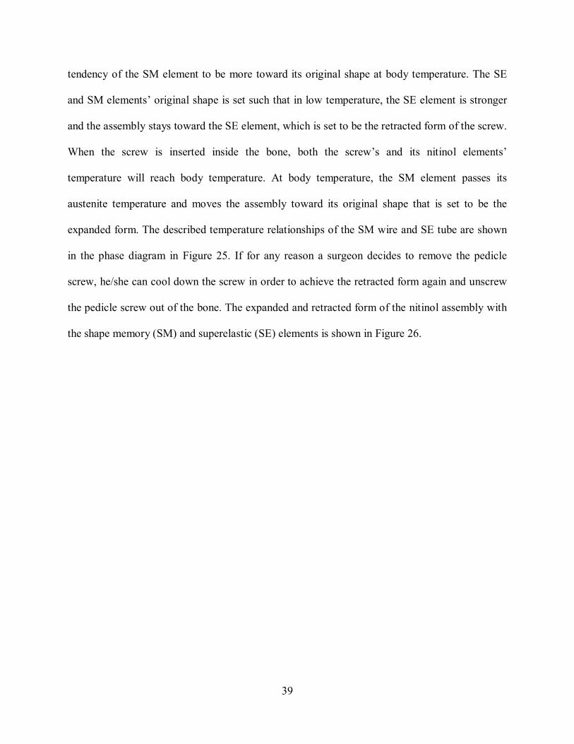
Figure 25- States of the SM and SE elements in their phase plot at inside and outside body temperature. The SM element is in martensite at outside body temperature and transforms to austenite phase in body temperature while the SE element is in austenite at inside body and outside body temperatures. ........................................................................................................ 40

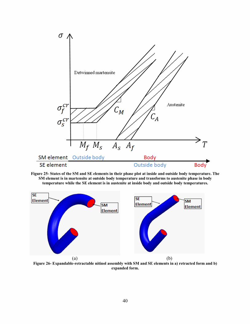
Figure 26- Expandable-retractable nitinol assembly with SM and SE elements in a) retracted form and b) expanded form. ...................................................................................................... 40

Figure 27- Schematic illustration of the problem solving in Abaqus with UMAT subroutine [5]51 Figure 28- Simulation results of tensile test in Abaqus against experiments by Gillet et al. [35] 57

Figure 29- Three point bending test beam dimensions ............................................................... 58 Figure 30- Stressdistribution on the beam .................................................................................. 59

Figure 31- Force versus displacement of the three point bending test in simulation against experimental results by Gillet et al. [35] .................................................................................... 59

Figure 32- BOSE Electroforce machine ..................................................................................... 60

ix

Figure 33- Tensile test experiment ............................................................................................ 61 Figure 34- Comparison of the 3-D model (developed in Abaqus) with the experimental axial stress-strain curve of 0.020” wire. ............................................................................................. 64 Figure 35- Comparison of torque-angle results of the model (developed in Abaqus) with the experimental data for various wire diameters (d=0.023, 0.020, 0.018 inch). ............................... 64 Figure 36- Shape Set form of the SE and SM elements. The elements are shape set in the opposite directions. ................................................................................................................... 65 Figure 37- dSPACE hardware ................................................................................................... 66

Figure 38- Laser distance sensor device (optoNCDT 1401) ....................................................... 67 Figure 39- Actuator assembly with the antagonistic SE and SM elements. The wire is connected to the two sides of the SM wire. ................................................................................................ 67 Figure 40- SIMULINK model to predict temperature. The model consist of the block to read from dSPACE input port (ADC) and the block to send signal to the output port (DAC) ............ 69 Figure 41- Input signals to heat the SM wire and the predicted temperature of the SM element due to the current input signals. The prediction was done Simulink® model by numerically solving the Joule heating differential equation. .......................................................................... 70

Figure 42- Actuator setup in room temperature.......................................................................... 71 Figure 43- Actuator setup in its high temperature. ..................................................................... 72

Figure 44- Measured displacement of the tip versus the temperature of the beam ...................... 73 Figure 46- Simulated mises stress distribution of the SM and SE elements in a) high temperature and b) low temperature form. .................................................................................................... 75 Figure 47- Temperature-displacement path of the actuator with the 5A current profile as the input. ......................................................................................................................................... 76 Figure 48- Temperature-displacement path of the actuator with the 6A current profile as the input. ......................................................................................................................................... 76 Figure 49- Schematic of test apparatus for pullout strength test from ASTM F543-02 standard . 77

Figure 50- Cross section profile of the employed 6:5mm cancellous bone screw with spherical under-surface and asymmetrical thread, derived from British Standard Institution [5] ............... 79

Figure 51- Meshed quarter screw and the surrounding bone in pullout simulation. .................... 80 Figure 52- Meshed screw and the expanded wire in pullout test simulation. .............................. 81

Figure 53- Results of pullout simulations of the pedicle screw in normal bone, osteoporotic bone, and with expanded wires. .......................................................................................................... 82

x

List of Tables

Table 1- Mechanical properties of bone [18] ............................................................................ 29 Table 2- Osteoporosis statistical information [23]...................................................................... 33

Table 3- Material properties of the niti rod ................................................................................ 62 Table 4- Implemented constants for prediction of temperature. .................................................. 68

Table 5- Material properties of the SM wire. ............................................................................. 73 Table 6- Employed pedicle screw dimensions in this study. All the dimensions are derived from [5] ............................................................................................................................................. 78 Table 7- Employed material properties for bone and screw........................................................ 78

xi

Nomenclature

����� Body temperature

���� Outside body temperature ���� Austenite final temperature of the supereleastic element

���� Martensite final temperature of the shape memeory element

���� Austenite final temperature of the shape memory element

� Gibbs free energy � Stress Tensor � Temperature � Martensitic volume fraction �� Transformation strain � Density � Compliance tensor � Thermal expansion coefficient �� Reference temperature � Specific heat coefficient �� Reference entropy state �� Reference internal energy state �(�) Hardening function �� Compliance tensor in austenite �� Compliance tensor in marteniste �� Thermal expansion in austenite �� Thermal expansion in austenite �� Specific heat coefficient in austenite �� Specific heat coefficient in martensite ��� Reference entropy state in austenite

��� Reference entropy state in martensite

��� Reference internal energy state in austenite

��� Reference internal energy state in austenite

�̇ Derivative of strain Λ Transformation tensor

�̇ Derivative of martensitic volume fraction � Maximum transformation strain in 3D ���� Strain at the reversal point � Transformation function � Thermodynamic force �∗ Internal dissipation due to phase transformation �� Austenite modulus of elasticity �� Marteniste modulus of elasticity �� Martensite finish temperature

�� Martensite start temperature �� Austenite start temperature

xii

�� Austenite finish temperature

�� Stress influence coefficient for transformation into martensite �� Stress influence coefficient for transformation into austenite ��� Stress at the start of transformation to martensite ��� Stress at the finish of transformation to martensite

��� Stress at the start of transformation to austenite ��� Stress at the finish of transformation to austenite

�� Maximum transformation strain in 1D �� Poisson’s ratio of martensite �� Poisson’s ratio of austenite � Resistivity � Electrical current ℎ� Heat convection coefficient �� Area of heat exchange ���� Ambient temperature

�� Specific heat capacity

�� Yield stress

12

Chapter One

Introduction

1.1. Shape memory alloys

Shape memory alloys belongs to a group of materials called active materials [1]. Active

materials are resulted from the extensive research over the past few decades on technologies in

engineering the mechanical, thermal and electrical properties of materials. Recently, active

materials have been used in different applications. Sensing is one of the applications in which the

material can convert the mechanical variation into a non-mechanical output. In actuation

applications, the material converts the non-mechanical input into the mechanical output. A group

of active materials including shape memory alloys and piezoceramics show direct coupling

behavior. In contrast, other active materials such as electo-rheological fluids (ERF) show indirect

coupling. This indirect coupling usually eliminates the reciprocity of the coupling behavior that

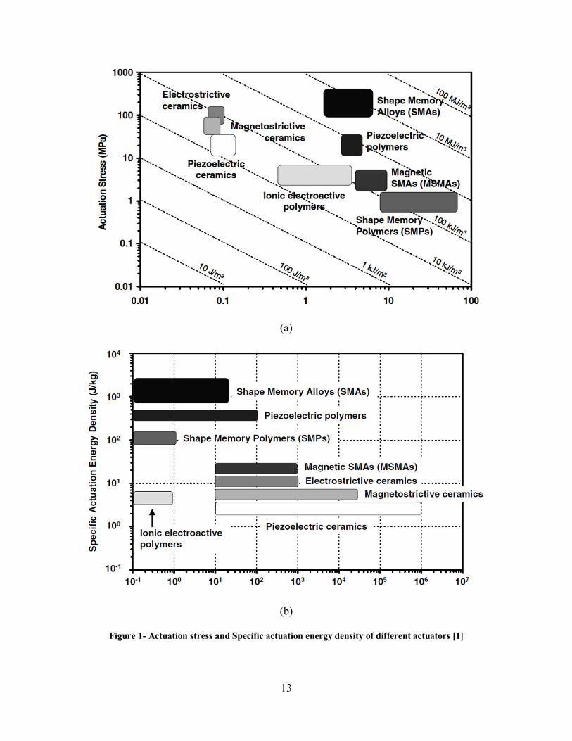
exists in other materials. For the actuation applications, two parameters play the most important

roles in the suitability of the active materials: actuation energy density, which is defined as the

available work output per unit volume, and the actuation frequency of the material. An ideal

actuator material is the one which has maximum actuation energy density and actuation

frequency. In Figure 1 these two parameters are shown for different materials.

13

(a)

(b)

Figure 1- Actuation stress and Specific actuation energy density of different actuators [1]

14

Shape memory alloys are a specific type of smart material which can recover their strain

upon heating. Increasing the temperature of the material results in recovery of the introduced

strain into the material even when the applied force is relatively large in a process known as

shape memory effect. This property makes the energy density high in shape memory alloys.

Also, under specific conditions, the material undergoes a hysteresis reversible transformation

which enables the material to dissipate energy for energy absorption applications. These

properties make shape memory alloys a good candidate for a variety of applications from

aerospace and automotive to biomedical. However, low frequency response of the material is a

disadvantage which restricts its applications.

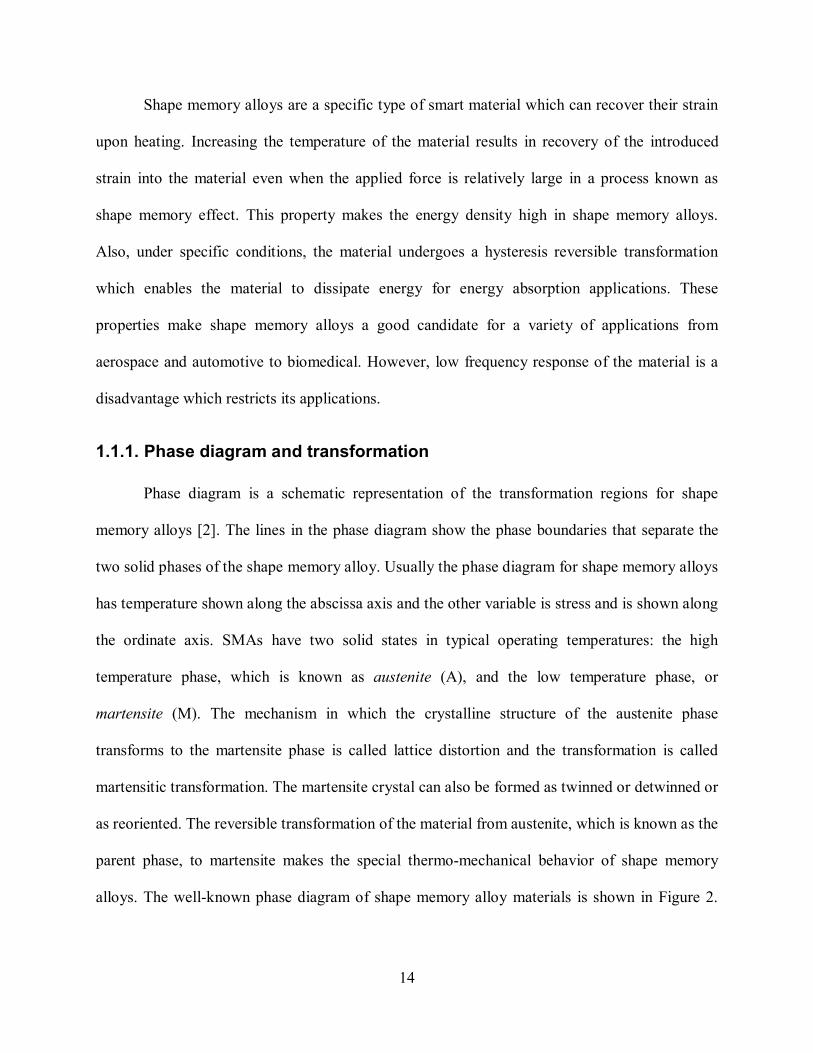
1.1.1. Phase diagram and transformation

Phase diagram is a schematic representation of the transformation regions for shape

memory alloys [2]. The lines in the phase diagram show the phase boundaries that separate the

two solid phases of the shape memory alloy. Usually the phase diagram for shape memory alloys

has temperature shown along the abscissa axis and the other variable is stress and is shown along

the ordinate axis. SMAs have two solid states in typical operating temperatures: the high

temperature phase, which is known as austenite (A), and the low temperature phase, or

martensite (M). The mechanism in which the crystalline structure of the austenite phase

transforms to the martensite phase is called lattice distortion and the transformation is called

martensitic transformation. The martensite crystal can also be formed as twinned or detwinned or

as reoriented. The reversible transformation of the material from austenite, which is known as the

parent phase, to martensite makes the special thermo-mechanical behavior of shape memory

alloys. The well-known phase diagram of shape memory alloy materials is shown in Figure 2.

15

The pseudoelasticity and shape memory effect as the special thermo-mechanical properties of

shape memory alloys are described in the following sections.

Figure 2- Phase diagram of a shape memory alloy material [2]. The austenite and martensite transformation bands are shown. The critical stresses and temperatures of the material are placed on the temperature and

stress axes.

1.1.2. Shape memory effect

Shape memory effect is the ability of the alloy to recover a certain amount of strain upon

heating [3]. This phenomenon happens when the material is loaded such that the structure

reaches the detwinned martensite phase and then unloaded while the temperature is below the

austenite final temperature (As). Heating the material at this stage will lead to strain recovery of

the material and the material will regain its original shape. This phenomenon can be better

understood in the combined stress-strain temperature diagram as shown in Figure 3. This

diagram shows the typical thermo-mechanical behavior of shape memory alloys.

16

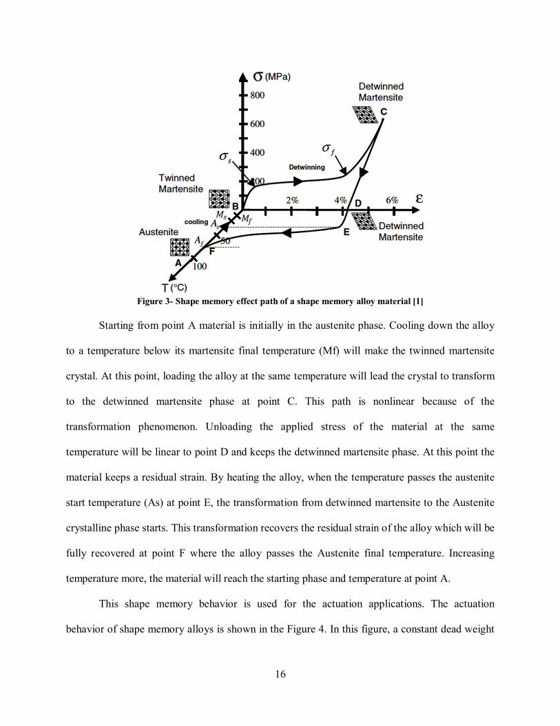
Figure 3- Shape memory effect path of a shape memory alloy material [1]

Starting from point A material is initially in the austenite phase. Cooling down the alloy

to a temperature below its martensite final temperature (Mf) will make the twinned martensite

crystal. At this point, loading the alloy at the same temperature will lead the crystal to transform

to the detwinned martensite phase at point C. This path is nonlinear because of the

transformation phenomenon. Unloading the applied stress of the material at the same

temperature will be linear to point D and keeps the detwinned martensite phase. At this point the

material keeps a residual strain. By heating the alloy, when the temperature passes the austenite

start temperature (As) at point E, the transformation from detwinned martensite to the Austenite

crystalline phase starts. This transformation recovers the residual strain of the alloy which will be

fully recovered at point F where the alloy passes the Austenite final temperature. Increasing

temperature more, the material will reach the starting phase and temperature at point A.

This shape memory behavior is used for the actuation applications. The actuation

behavior of shape memory alloys is shown in the Figure 4. In this figure, a constant dead weight

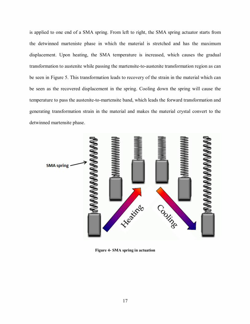
17

is applied to one end of a SMA spring. From left to right, the SMA spring actuator starts from

the detwinned marteniste phase in which the material is stretched and has the maximum

displacement. Upon heating, the SMA temperature is increased, which causes the gradual

transformation to austenite while passing the martensite-to-austenite transformation region as can

be seen in Figure 5. This transformation leads to recovery of the strain in the material which can

be seen as the recovered displacement in the spring. Cooling down the spring will cause the

temperature to pass the austenite-to-martensite band, which leads the forward transformation and

generating transformation strain in the material and makes the material crystal convert to the

detwinned martensite phase.

Figure 4- SMA spring in actuation

18

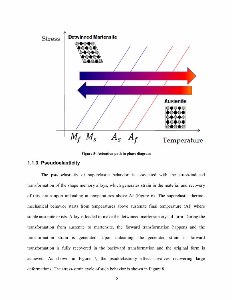
Figure 5- Actuation path in phase diagram

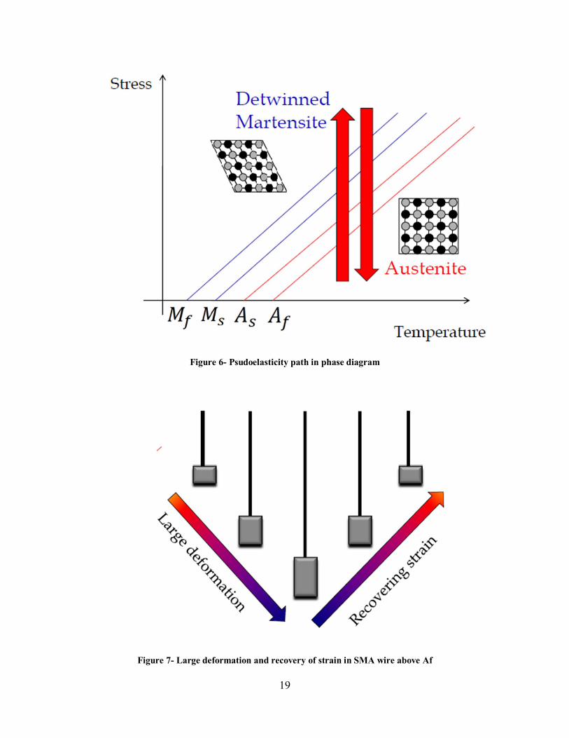
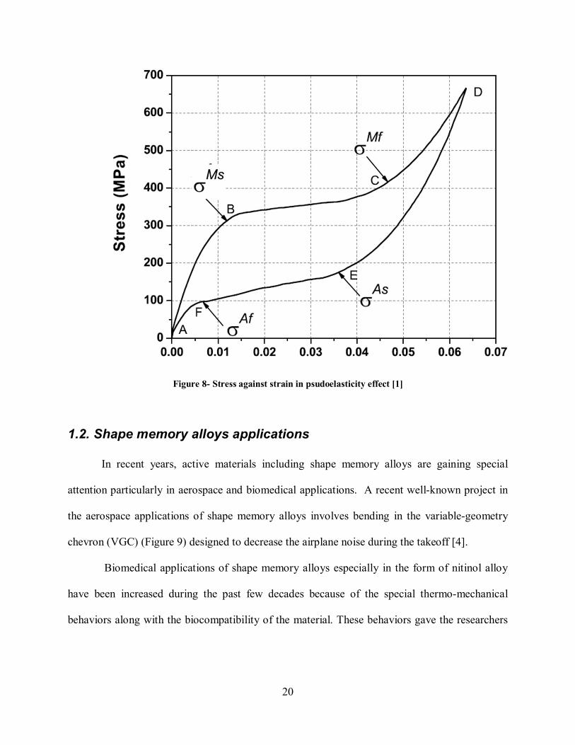
1.1.3. Pseudoelasticity

The psudoelasticity or superelastic behavior is associated with the stress-induced

transformation of the shape memory alloys, which generates strain in the material and recovery

of this strain upon unloading at temperatures above Af (Figure 6). The superelastic thermo-

mechanical behavior starts from temperatures above austenite final temperature (Af) where

stable austenite exists. Alloy is loaded to make the detwinned martensite crystal form. During the

transformation from austenite to martensite, the forward transformation happens and the

transformation strain is generated. Upon unloading, the generated strain in forward

transformation is fully recovered in the backward transformation and the original form is

achieved. As shown in Figure 7, the psudoelasticity effect involves recovering large

deformations. The stress-strain cycle of such behavior is shown in Figure 8.

19

Figure 6- Psudoelasticity path in phase diagram

Figure 7- Large deformation and recovery of strain in SMA wire above Af

20

Figure 8- Stress against strain in psudoelasticity effect [1]

1.2. Shape memory alloys applications

In recent years, active materials including shape memory alloys are gaining special

attention particularly in aerospace and biomedical applications. A recent well-known project in

the aerospace applications of shape memory alloys involves bending in the variable-geometry

chevron (VGC) (Figure 9) designed to decrease the airplane noise during the takeoff [4].

Biomedical applications of shape memory alloys especially in the form of nitinol alloy

have been increased during the past few decades because of the special thermo-mechanical

behaviors along with the biocompatibility of the material. These behaviors gave the researchers

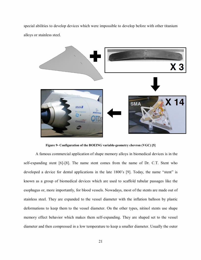
21

special abilities to develop devices which were impossible to develop before with other titanium

alloys or stainless steel.

Figure 9- Configuration of the BOEING variable-geometry chevron (VGC) [5]

A famous commercial application of shape memory alloys in biomedical devices is in the

self-expanding stent [6]- [8]. The name stent comes from the name of Dr. C.T. Stent who

developed a device for dental applications in the late 1800’s [9]. Today, the name “stent” is

known as a group of biomedical devices which are used to scaffold tubular passages like the

esophagus or, more importantly, for blood vessels. Nowadays, most of the stents are made out of

stainless steel. They are expanded to the vessel diameter with the inflation balloon by plastic

deformations to keep them to the vessel diameter. On the other types, nitinol stents use shape

memory effect behavior which makes them self-expanding. They are shaped set to the vessel

diameter and then compressed in a low temperature to keep a smaller diameter. Usually the outer

22

diameter of the shape set form is set 10% larger to assure that the stent cannot move. These

stents are usually made by laser cutting a tube to make the latticed wall. But more than the shape

memory effect, the superelasticity of the nitinol stents inside the body is another strong point for

them. This gives them the flexibility of 10 to 20 times more than stainless steel. This flexibility is

an important property in some superficial applications where the stent may be subjected to

outside deformation or pressure. These deformations in stainless steel stents can cause permanent

deformations and serious consequences for the patients while the superelasticity effect in nitinol

stents makes them a much better option in superficial applications.

The reasons that nitinol has been widely used in medical applications are listed as

below [6].

Elastic deployment

Thermal deployment

Kink resistance

Biocompatibility

Constant unloading stresses

Biomechanical compatibility

Dynamic interference

Hysteresis

MR compatibility

Fatigue resistance

Uniform Plastic deformation

Elastic deployment or the extra flexibility of nitinol, which is the reason of the super-elasticity

effect, can be used for different medical devices. Some devices need an instrument that can move

23

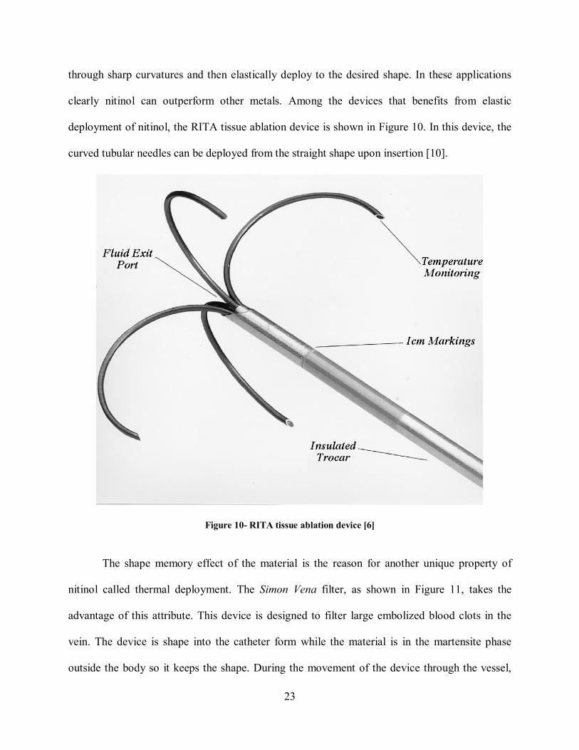
through sharp curvatures and then elastically deploy to the desired shape. In these applications

clearly nitinol can outperform other metals. Among the devices that benefits from elastic

deployment of nitinol, the RITA tissue ablation device is shown in Figure 10. In this device, the

curved tubular needles can be deployed from the straight shape upon insertion [10].

Figure 10- RITA tissue ablation device [6]

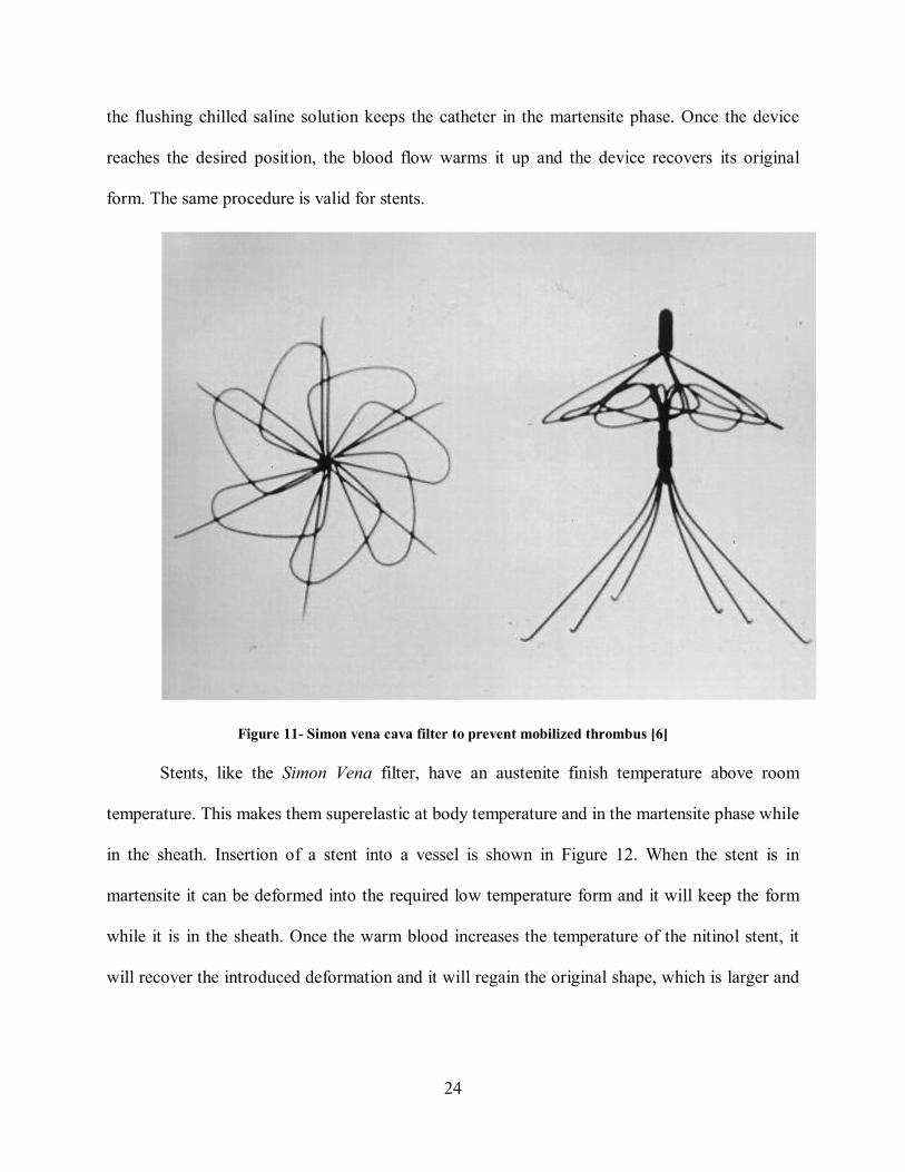
The shape memory effect of the material is the reason for another unique property of

nitinol called thermal deployment. The Simon Vena filter, as shown in Figure 11, takes the

advantage of this attribute. This device is designed to filter large embolized blood clots in the

vein. The device is shape into the catheter form while the material is in the martensite phase

outside the body so it keeps the shape. During the movement of the device through the vessel,

24

the flushing chilled saline solution keeps the catheter in the martensite phase. Once the device

reaches the desired position, the blood flow warms it up and the device recovers its original

form. The same procedure is valid for stents.

Figure 11- Simon vena cava filter to prevent mobilized thrombus [6]

Stents, like the Simon Vena filter, have an austenite finish temperature above room

temperature. This makes them superelastic at body temperature and in the martensite phase while

in the sheath. Insertion of a stent into a vessel is shown in Figure 12. When the stent is in

martensite it can be deformed into the required low temperature form and it will keep the form

while it is in the sheath. Once the warm blood increases the temperature of the nitinol stent, it

will recover the introduced deformation and it will regain the original shape, which is larger and

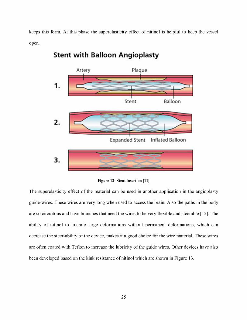
25

keeps this form. At this phase the superelasticity effect of nitinol is helpful to keep the vessel

open.

Figure 12- Stent insertion [11]

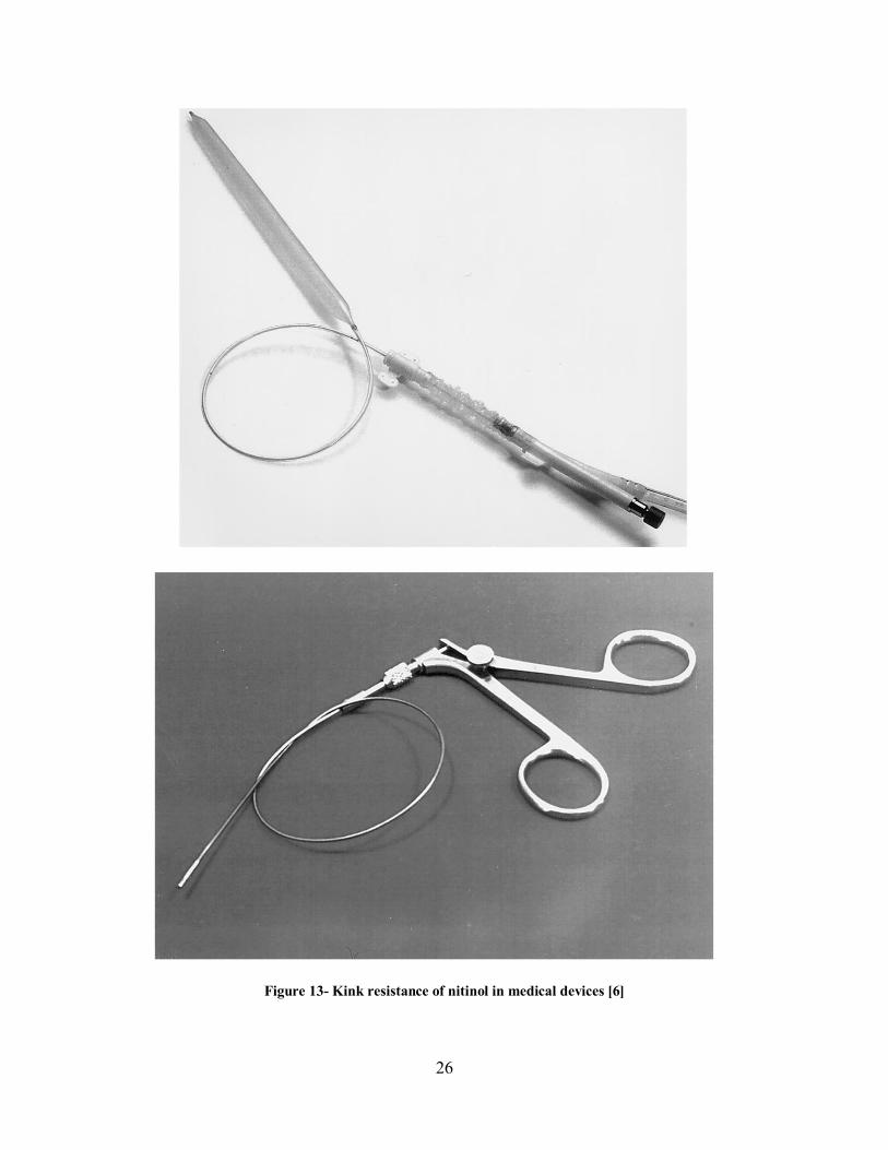
The superelasticity effect of the material can be used in another application in the angioplasty

guide-wires. These wires are very long when used to access the brain. Also the paths in the body

are so circuitous and have branches that need the wires to be very flexible and steerable [12]. The

ability of nitinol to tolerate large deformations without permanent deformations, which can

decrease the steer-ability of the device, makes it a good choice for the wire material. These wires

are often coated with Teflon to increase the lubricity of the guide wires. Other devices have also

been developed based on the kink resistance of nitinol which are shown in Figure 13.

26

Figure 13- Kink resistance of nitinol in medical devices [6]

27

The amount of body reaction when an external material is placed inside the body defines the

biocompatibility of a material. Researchers have reported an extremely good biocompatibility for

the nitinol material because of formation of ���� layer and very similar to �� alloy inside the

body [13]- [17]. Another aspect of the biocompatibility of nitinol is shown in Figure 14. As can

be seen, the Ptentiodynamics results show that the biocompatibility of nitinol is between Ti6-6-4

AND 316l.

Figure 14- Nitinol potential is between Ti-6-4 and 316L [6]

By looking into the stress strain plot of Titanium and Stainless Steel, it is understood

clearly that they are stiffer and not similar to the plots for biological materials. Unlike these

28

metals, nitinol has a very similar mechanical behavior to the biological materials. The stress-

strain plots as shown in Figure 15 have similar hysteresis.

Figure 15- Stress-Strain curve of a few biological materials and comparison to nitinol 87 [6]

This property gives nitinol the ability to distribute the load with the surrounding tissue

and promote the growth of the surrounding bone. A group of orthopedic devices like the bone

staples and hip implants take advantage of this property.

One other property of nitinol is the MR compatibility. Researchers have reported that

nitinol shows a clear image better than stainless steel and similar to pure titanium [6]. A MR

29

image of a stent is shown in Figure 16. As can be seen, the stent shape is very clear in the MR

image.

Figure 16- MRI compatibility nitinol in stent [6]

1.3. Pedicle screw in osteoporotic bone

1.3.1. Spinal bone

The spinal bone has both the cortical and trabecular parts. The cortical bone is compact with

about 1.8 g/cm^3 density. Dissimilarly, the trabecular bone is cancellous with 0.01-0.9 g/cm^3

density. The cortical bone has mechanical properties which have been listed in Table 1.

Table 1- Mechanical properties of bone [18]

Ultimate strength

(Mpa)

Elastic modulus

(Gpa)

Tension 92-188 7.1-28.2

30

Compression 133-295 14.7-34.3

Torsion 53-76 3.1-3.7

The Trabecular bone has a cancellous structure with vertical and horizontal fibers. According to

the experiments, depending on the direction of the applied load, the mechanical properties of the

bone change. Also the researchers have reported that the strength of the cancellous bone is 60%-

70% more in compression in comparison to tension [18]. The differences of the Trabecular bone

and Cortical bone are illustrated in Figure 17.

Figure 17- Trabecular and Cortical bone [19]

31

1.3.2. Pedicle screw

Bone screws for various spinal treatments and fixations have been used for about 70

years [20]. Pedicle screws are used in vertebral column fixation and treatments. Pedicle is the

small bony area, on either side of the vertebral body. Pedicles are the connection member of the

vertebral body to the arch (Figure 18). Pedicle screws are used as bone anchoring elements to

firmly grip the bone to facilitate attachment to the spinal implants.

Figure 18- Vertebrae anatomy [21]

Pedicle screws themselves don’t fix the spine in one place. Usually a connection rod is

used to firmly connect these screws, which are inserted into two or three spinal segments (Figure

19). Using the pedicle screws and the connection rod, surgeons can fix the spinal segments

together for spinal fusion. Due to the pedicle’s high density in healthy bones and its special

structure, it makes it a good place for screw placement. The pedicular fixation system (which

consists of a minimum of four pedicle screws and the rods) can resist against large loads and

stabilize a fractured spine. These loads require the pedicle screws to be tightly fixed to the

pedicle bone. Medical applications of pedicle screws show that tolerating the applied forces is

possible for pedicle screws inside a healthy bone. When the bone is not healthy, poor screw

32

purchase becomes the main concern [25].

(a) (b)

(c) (d) Figure 19- Pedicle screw fixation. a) Pedicle screws implanted into the pedicle area. b) pedicle screw and the connection rod and c),d) pedicle screw and the connection rod implanted into the pedicle bone to fixate the

spine and correct deformity [23], [24]

33

1.3.3. Osteoporosis and its adverse effect in bone fixations

Osteoporosis is a very common bone disease in elderly people and especially in females which

increases the risk of fracture in the bones of the patients. In this disease, the bone mineral density

(BMD), which is related to the amount of the minerals in a certain volume, decreases drastically.

The occurrence of this disease in elderly people steeply increases with age.

The National Osteoporosis Foundation (NOF) estimates that there are approximately 10

million people living in the United States who suffer from osteoporosis [27]. Approximately

80% of them are women. An additional 34 million U.S. citizens are considered at risk of

developing osteoporosis due to having low bone mass. Statistical information regarding the

prevalence and risk of osteoporosis among different demographics is presented in Table 2. The

statistics pertain to individuals who are over the age of 50 years.

There are some methods to measure the level of osteoporosis in patients. One of them is

the Jikei osteoporosis Grading Scale which is based on radiographic images [28], [29]. Figure 20

shows the radiographic images of the patient’s spine from healthy bone to osteoporosis Grade 3.

The image of the Grade 3 osteoporosis clearly shows that the bone is disappeared and the density

is reduced.

Table 2- Osteoporosis statistical information [27]

34

Figure 20- Ostoprosis bone grade in radiographic images [28], [29]

For the surgeon, when deciding on the use of bone fixations for patients, the main concern is

patients’ bone quality. Poor bone quality will cause loosening of the bone fixation during or after

surgery. The bone’s poor quality in osteoporosis for the pedicle bone is shown in Figure 21.

Figure 21- Osteoporosis in pedicle bone [30]

35

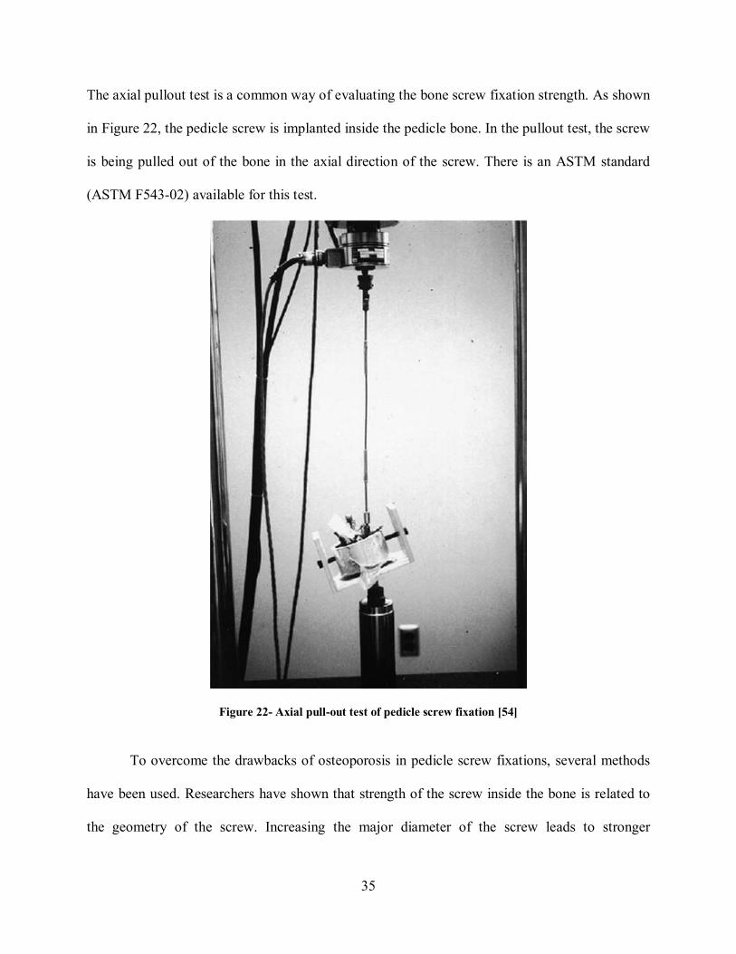
The axial pullout test is a common way of evaluating the bone screw fixation strength. As shown

in Figure 22, the pedicle screw is implanted inside the pedicle bone. In the pullout test, the screw

is being pulled out of the bone in the axial direction of the screw. There is an ASTM standard

(ASTM F543-02) available for this test.

Figure 22- Axial pull-out test of pedicle screw fixation [54]

To overcome the drawbacks of osteoporosis in pedicle screw fixations, several methods

have been used. Researchers have shown that strength of the screw inside the bone is related to

the geometry of the screw. Increasing the major diameter of the screw leads to stronger

36

engagement of screw and bone. Chapman et al. [55] also showed that thread geometry has a

significant effect on the pullout force of pedicle screws. The procedure of fitting the screw to the

bone also has an effect on the pullout force. Battula et al [56] developed a parameter based on

the pilot-hole size drilled into the bone before pedicle screw insertion. They showed that holes

with a diameter larger than 72% of the screw’s outer diameter had an adverse effect on the

pullout test.

One of the methods that showed successful treatment in mitigating the osteoporosis

adverse effect was to inject a special kind of bio-compatible cement through the screw in order to

glue the screw to the surrounding bone [57], [58], [59]. Even though this method has shown

good performance in pullout tests, it poses several disadvantages which restrict its application.

The hardening process of one common type of these cements (called Poly methyl methacrylate

or PMMA), is an exothermic reaction releasing unwanted heat to the surrounding areas. This

heat can be dangerous since the areas in question are so close to the neural elements of the spine.

Also, the cement poses the threat of causing an infection around the pedicle bone. Lastly,

applying the cement makes it much more difficult to remove the pedicle screw in the future,

which may be necessary in the case of revision surgery. Another method is to use

Hydroxyapatite coated implants. Both experimental and clinical research have shown higher

bone screw purchase than the uncoated pedicle screws [60].

Recent research has shown novel methods that take advantage of expandable elements

that increase the strength of the connection between screw and bone [61], [62]. The expandable

form of dental implants is the other application of the expandable screws [63]. The elements in

these screws are only expandable (and not retractable) so that the removal of the screw becomes

a much more challenging problem.

37

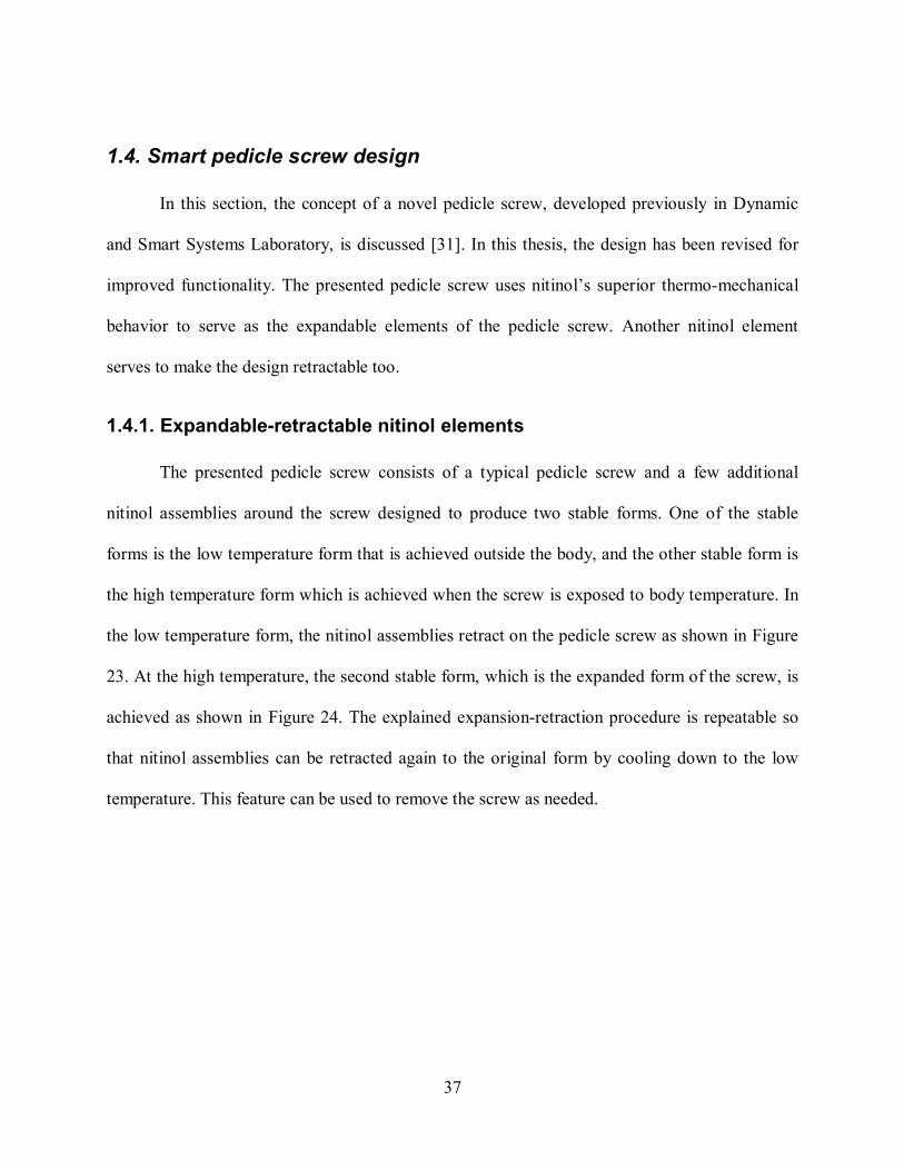
1.4. Smart pedicle screw design

In this section, the concept of a novel pedicle screw, developed previously in Dynamic

and Smart Systems Laboratory, is discussed [31]. In this thesis, the design has been revised for

improved functionality. The presented pedicle screw uses nitinol’s superior thermo-mechanical

behavior to serve as the expandable elements of the pedicle screw. Another nitinol element

serves to make the design retractable too.

1.4.1. Expandable-retractable nitinol elements

The presented pedicle screw consists of a typical pedicle screw and a few additional

nitinol assemblies around the screw designed to produce two stable forms. One of the stable

forms is the low temperature form that is achieved outside the body, and the other stable form is

the high temperature form which is achieved when the screw is exposed to body temperature. In

the low temperature form, the nitinol assemblies retract on the pedicle screw as shown in Figure

23. At the high temperature, the second stable form, which is the expanded form of the screw, is

achieved as shown in Figure 24. The explained expansion-retraction procedure is repeatable so

that nitinol assemblies can be retracted again to the original form by cooling down to the low

temperature. This feature can be used to remove the screw as needed.

38

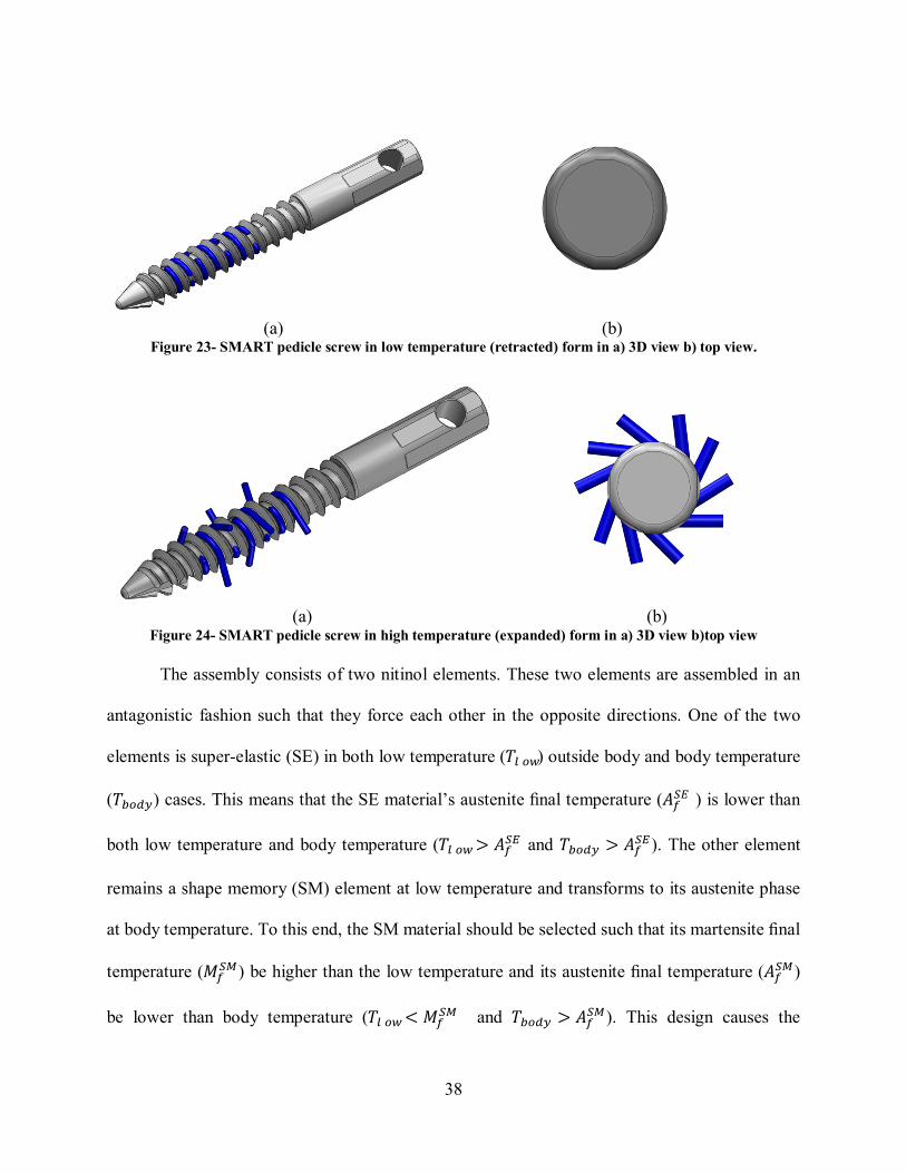
(a) (b) Figure 23- SMART pedicle screw in low temperature (retracted) form in a) 3D view b) top view.

(a) (b) Figure 24- SMART pedicle screw in high temperature (expanded) form in a) 3D view b)top view

The assembly consists of two nitinol elements. These two elements are assembled in an

antagonistic fashion such that they force each other in the opposite directions. One of the two

elements is super-elastic (SE) in both low temperature (����) outside body and body temperature

(�����) cases. This means that the SE material’s austenite final temperature (���� ) is lower than

both low temperature and body temperature (����> ���� and ����� > ��

��). The other element

remains a shape memory (SM) element at low temperature and transforms to its austenite phase

at body temperature. To this end, the SM material should be selected such that its martensite final

temperature (����) be higher than the low temperature and its austenite final temperature (��

��)

be lower than body temperature (����< ���� and ����� > ��

��). This design causes the

39

tendency of the SM element to be more toward its original shape at body temperature. The SE

and SM elements’ original shape is set such that in low temperature, the SE element is stronger

and the assembly stays toward the SE element, which is set to be the retracted form of the screw.

When the screw is inserted inside the bone, both the screw’s and its nitinol elements’

temperature will reach body temperature. At body temperature, the SM element passes its

austenite temperature and moves the assembly toward its original shape that is set to be the

expanded form. The described temperature relationships of the SM wire and SE tube are shown

in the phase diagram in Figure 25. If for any reason a surgeon decides to remove the pedicle

screw, he/she can cool down the screw in order to achieve the retracted form again and unscrew

the pedicle screw out of the bone. The expanded and retracted form of the nitinol assembly with

the shape memory (SM) and superelastic (SE) elements is shown in Figure 26.

40

Figure 25- States of the SM and SE elements in their phase plot at inside and outside body temperature. The

SM element is in martensite at outside body temperature and transforms to austenite phase in body temperature while the SE element is in austenite at inside body and outside body temperatures.

(a) (b) Figure 26- Expandable-retractable nitinol assembly with SM and SE elements in a) retracted form and b)

expanded form.

41

1.5. Objectives The main objective of the research is to verify the concept of the new pedicle screw. To be able

to verify the concept of the designed expandable and retractable elements, a framework is needed

to numerically simulate the behavior. Like other numerical tools, the results of the simulation

need to be verified before being used in design and optimization. To this end a set of experiments

are required to verify the model

The other objective is to evaluate the performance of the expandable elements in

mitigating the osteoporosis adverse effect in the bone fixation. Similarly finite element software

can be used to evaluate the performance.

1.6. Approach To achieve the desired objectives, the first step is to be able to numerically simulate the

performance of the designed shape memory alloy expandable-retractable attached to the pedicle

screw to mitigate osteoporosis effect in bone fixation. To this end, the numerical form of a three

dimensional thermo-mechanical model of shape memory alloys, which is coded in Abaqus

UMAT subroutine, is used. The numerical tool is able to capture the shape memory effect and

pseudoelasticity in three dimensional geometries. This simulation tool is used to verify the

concept of the designed elements which can expand and retract around the shaft of a pedicle

screw. The model for this actuation system in larger scales is made in Abaqus and validated

through the experiment to verify the concept.

The other objective was to verify the effect of the expanded element around the pedicle

screw and show the higher purchase of the bone fixation. Another model is prepared in Abaqus

to numerically simulate the bone screw strength and verify the performance.

42

1.7. Contributions The contribution of the work was to be able to successfully simulate the three dimensional

thermo-mechanical behaviors of the shape memory alloys in the biomedical device. The

performance of the finite element numerical code in Abaqus UMAT subroutine is verified for the

biomedical devices applications with experiments. More than that, another model is developed in

Abaqus finite element software to predict the performance of the designed novel pedicle screw in

pullout test. The following publications are the results of the efforts during this research.

1.8. Publications Journal

1. Eshghinejad, A. and Elahinia, M.,”Functionality evaluations of a novel expandable pedicle

screw to mitigate osteoporosis effect in bone fixations: modeling and experimentation”, Journal

of Biomechanics, (submitted)

2. Anderson, W., Eshghinejad, A. and Elahinia, M., “Transverse Load Capacity at Mid-Span of

Heat-Treated nitinol and Finite Element Predictions”, Journal of Smart Materials and

Structures, (submitted)

3. A. Eshghinejad, M. Elahinia, “Exact solution for bending of shape memory alloy beams”,

Journal of Smart Materials and Structures, (submitted)

4. Chapman, C., Eshghinejad, A. and Elahinia, M., “Torsional Behavior of Shape Memory

Wires and Tubes: Modeling and Experimentation”, Journal of Intelligent Material Systems and

Structures, July 2011, 22(11):1239-1248.

Proceeding

1. Anderson, W., Eshghinejad, A. and Elahinia, M., “An Organ Positioner to Mitigate

43

Collateral Tissue Damage in Esophagus during Atrial Fibrilation”, Design of Medical Devices

Conference, April 10-12, Minneapolis, Minnesota

2. Anderson, W., Eshghinejad, A. and Elahinia, M., “Transverse Load Capacity at Mid-Span of

Heat-Treated nitinol and Finite Element Predictions”, Material Science & Technology

Conference, October 16-20 Columbus, Ohio

3. A. Eshghinejad, M. Elahinia, M. Tabesh, “A novel expandable pedicle screw to mitigate

Osteoporosis”, ASME 2011 Conference on Smart Materials Adoptive Structures and Intelligent

Systems, September, Arizona 2011

4. W. Anderson, A. Eshghinejad, M. Elahinia, “Material characterization and mid-span bending

capacity with finite element simulated predictions”, ASME 2011 Conference on Smart

Materials Adoptive Structures and Intelligent Systems, September, Arizona 2011

5. A. Eshghinejad, M. Elahinia, “Exact solution for bending of shape memory alloy superelastic

Beams”, ASME 2011 Conference on Smart Materials Adoptive Structures and Intelligent

Systems,September, Arizona 2011

6. A. Eshghinejad, M. Elahinia,”Functionality analysis of nitinol elements in expandable pedicle

screw to mitigate osteoporosis”, Midwest Graduate research symposium, the University of

Toledo, 2011

Report

Business plan report: “SMArt pedicle screw production and marketing analysis”, Annual UTIE

Business Plan Competition at the University of Toledo, OH, October 2011

44

Chapter Two

Mathematical modeling of shape memory alloys and the numerical implementation

2.1. Introduction

In order to completely understand the thermo-mechanical behavior of shape memory

alloys in any application, developing mathematical models is inevitable. During the recent years

the area of constitutive modeling of shape memory alloys has been the point of interest of many

researchers. The developed models can be classified into two groups: Micromechanical-based

models and phenomenological models [32].

The micromechanical models use the polycrystalline behavior of SMAs in martensite and

austenite. These models develop the mathematical thermo-mechanical models in the microscopic

viewpoint.

The phenomenological models assume the mixture of two solid state phases to represent

the behavior of the material. Preisach models [33] and the irreversible thermodynamics

principles [34] can be listed among these models. These modeling use different energy

conservation principles. Most of the parameters along with the state variables in the

phenomenological models are easy to measure. This makes these models easier to use in

application and the numerical implementations.

45

Tanaka and Nagaki [35] model was among the first phenomenological models presented.

The state variables in this model were strain (�) and temperature (T) and the martensite volume

fraction which has a value between zero and one (0 < � < 1). The internal variables were

assumed be time and space averaged on the material domain. The model developed by Liang and

Rogers [36] in later years and followed by Brinson models [37] [38] [39] and added the twinned

and detwinned Martensite as another internal variable to model the behavior based on an

experimentally defined phase diagram. It was shown that various one dimensional

phenomenological models are similar but they are different in formulations of the transformation

functions [38]. Later Gao et al. [39] improved the previous works by developing a one

dimensional finite element method for truss elements, utilized to model shape memory alloys

behavior in several models.

Modeling and analysis of SMA beams in bending has been the subject of several

investigations. Gillet et al. [40] developed a numerical method to predict the behavior of a SMA

beam in a three-point bending test. They conducted experiments for validating the numerical

results. M. Jaber et al. [41] used finite element analysis to predict SMA beam behavior in a

nitinol staple. Hartl et al. [42], [43] addressed the training, characterization, and derivation of the

material properties of their shape memory alloy actuator. They also assessed the actuation

properties of their active beam actuator and analyzed it accurately using finite element analysis.

They developed a numerical tool in Abaqus to simulate the actuator's thermo- mechanical

behavior. Tabesh et al. [44] used a combined SMA rod and tube assembly in bending. They used

the shape memory effect and superelastic behavior of nitinol alloy to develop a bi-stable

actuator. In their actuator the tube and rod apply bending force in an antagonistic manner as a

46

result of temperature variation. Mineta et al. [45] used a SMA bending beam to develop a micro-

actuator. Zbiciak performed dynamic analysis for superelastic beams [46].

While numerical methods are widely used and accepted for analyzing SMA devices, they

have certain limitations. Validity of the results is always a concern, which necessitates

experimental validation. It is a known fact that experimentation with these alloys, even for

simple tests, is difficult and could be expensive. It is desirable that the numerical solutions can be

validated against closed-form solutions [47]. Exact solutions are less expensive computationally

and as a result they provide faster simulations. Additionally, exact models are more readily

applicable in real time simulations and control of SMA actuators. Mirzaefar et al. [47] have

conducted a study to find the exact solution for torsional behavior of shape memory alloy bars.

They simplified a three dimensional model [67] to a one-dimensional shear form. This way, they

developed an exact form for the relationship between the applied torque and the angular

displacement. Two studies [48], [49] proposed an analytical solution for solving the moment due

to stress distribution of a superelastic material versus the curvature of a SMA Euler-Bernoulli

beam. The limitation of these solutions is due to assuming equal elastic moduli for austenite and

martensite phases of the material. The other limitation is assuming equal initial and final stresses

for the phase transformation values. This assumption is not exactly what we usually observe in

tensile tests of SMA specimens.

In the next section one of the famous phenomenological constitutive models of shape

memory alloys which were used in this work will be described. The numerical implementation of

the model in Abaqus as the finite element software is also described.

47

2.2. Boyd-Lagoudas constitutive model for shape memory alloys

The model presents a three dimensional thermo-mechanical constitutive model for shape

memory alloys. The model has been extensively explained in Lagoudas et al. [66]. In this

section the model is briefly described which will be used for the following simulations.

The model is based on the Gibbs free energy as given by:

�(�, �, �, ��) = −1

2

1

��: �: � −

1

��: [�(� − ��) + �

�] + � �(� − ��) − ��� ��

����

− ��� + �� + �(�)

(1)

where �, �, ��, � and �� are defined as the Cauchy stress tensor, martensitic volume fraction,

transformation strain tensor, current temperature and reference temperature, respectively. Other

material constants�, �, �,�, �� and �� are the effective thermal expansion tensor, effective

compliance tenser, density, effective specific heat, and effective specific internal energy at

reference state and effective entropy at reference state. The hardening function was shown in the

equation as�(�). As described in Lagoudas [1], by setting the hardening function in the

available models different hardening curves can be achieved. These material constants are

defined with rule of mixture in the material.

� = �� + �(�� − ��) (2)

� = �� + �(�� − ��) (3)

� = �� + �(�� − ��) (4)

� = �� + �(�� − ��) (5)

�� = ��� + �(��

� − ���) (6)

�� = ��� + �(��

� − ���) (7)

48

The variables with superscripts A and M show the values in austenite and martensite

phases respectively. Based on the continuum mechanics equations to find the strain derived by

the energy, the total strain will be found as:

� = �: � + �(� − ��) + �� (8)

The first term is related to the strain due to the applied stress and the second term is the

strain due to thermal expansion and the last term is the strain due to transformation. This

equation requires a relationship between the transformation strain tensor �� and the marteniste

volume fraction. This relationship is expressed by:

�̇ = Λ�̇ (9)

In this equation, the transformation tensor is Λ which defines the direction of

transformation. Two different forms are proposed for the transformation tensor. The first one is:

Λ = �

3

2���

��, �̇ > 0

�����/�̅��� , �̇ < 0

(10)

where � is the maximum axial transformation strain, and ����is the transformation strain at the

reversal point. Other parameters are defined as:

�� = �3

2‖��‖ (11)

�� = � −1

3��(�)� (12)

�̅��� = �2

3‖����‖ (13)

This transformation tensor is suitable for proportional loading cases. For more complicated cases

a transformation tensor independent of the loading direction is defined as below for loading and

unloading cases:

49

Λ =3

2���

�� (14)

A new parameter named as thermodynamic force is defined on the second thermodynamic law

inequality in order to later recognize the transformation happening recognition.

� = �:Λ +1

2�: Δ�: � + Δ�: �(� − ��) − �Δ�[(� − ��) − ���(

�

��)] (15)

where prefix Δshows difference of the parameter value in martensite and austenite. Based on the

thermodynamic force the transformation function can also be defined as:

� = �� − �∗ �̇ ≥ 0

−� − �∗ �̇ ≤ 0 (16)

In this equation �∗is a constant and mentioned as the internal dissipation due to the phase

transformation. Using the second thermodynamic law from the Gibbs free energy, the following

inequalities can be derived:

�(�, �, �) ≤ 0 →�� = 0 ���̇ ≠ 0

� < 0 ���̇ = 0 (17)

This means that when the transformation is happening the � function needs to be equal to zero

and when there is no transformation in the material the � function needs to be less than zero. The

hardening functions which were mentioned in Equation 1 can be defined in several forms. The

Tanaka [50] form of the hardening function is selected as:

�(�) =

⎩⎨

⎧Δ�����

[(1 − �) ln(1 − �) + �] + (��� + ��

�)� �̇ > 0

−Δ�����

�[ln(�) − 1] + (��� + ��

�)� �̇ < 0

(18)

and the Liang and Rogers form of the function can be selected as:

50

�(�) =

⎩⎪⎨

⎪⎧� −

�����

�� − �����(2�� − 1)���� + (��� + ��

�)��

�

�̇ > 0

� −Δ������� − �����(2�� − 1)���� + (��

� + ���)�

�

�

�̇ < 0

(19)

The Boyd-Lagoudas [66] form is a polynomial form as:

�(�) = �

1

2����� + (��

�+ ��

�)� �̇ > 0

1

2����� + (��

�+ ��

�)� �̇ < 0

(20)

where the constants can be achieved to enforce the continuity of the function during forward and

backward transformation. Another hardening function is developed by Hartl [5] known as

smooth hardening function.

�̇� = �̇ �

1

2��(1 + �

�� − (1 − �)��) + �� �̇ > 0

1

2��(1 + �

�� − (1 − �)��) + �� �̇ < 0

= �̇ ������ �̇ > 0

����� �̇ < 0

(21)

In this form of the hardening function, the parameters �� define the degrees of smoothness.

2.3. Numerical implementation of the model in Abaqus

The described constitutive model to predict the behavior of shape memory alloy materials

cannot be used to model various geometries and conditions without implementation into a

numerical environment. To be able to have the capability of analyzing complex problems, a

previously developed code into the Abaqus finite Framework [51] as a user material subroutine

(UMAT) is used. This code is the numerical implementation of the described constitutive model.

The method in which the global Abaqus solver uses the UMAT subroutine to model a nonlinear

material like shape memory alloys is described in Figure 27. As shown, the model uses

displacement based FEA, which is known as the more popular method. Based on the thermo-

mechanical loading pass, solver begins by guessing the appropriate initial deformation over the

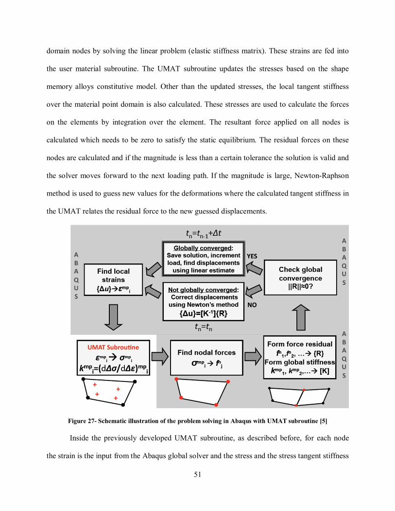
51

domain nodes by solving the linear problem (elastic stiffness matrix). These strains are fed into

the user material subroutine. The UMAT subroutine updates the stresses based on the shape

memory alloys constitutive model. Other than the updated stresses, the local tangent stiffness

over the material point domain is also calculated. These stresses are used to calculate the forces

on the elements by integration over the element. The resultant force applied on all nodes is

calculated which needs to be zero to satisfy the static equilibrium. The residual forces on these

nodes are calculated and if the magnitude is less than a certain tolerance the solution is valid and

the solver moves forward to the next loading path. If the magnitude is large, Newton-Raphson

method is used to guess new values for the deformations where the calculated tangent stiffness in

the UMAT relates the residual force to the new guessed displacements.

Figure 27- Schematic illustration of the problem solving in Abaqus with UMAT subroutine [5]

Inside the previously developed UMAT subroutine, as described before, for each node

the strain is the input from the Abaqus global solver and the stress and the stress tangent stiffness

52

are the outputs. The UMAT algorithm assumes no transformation at the beginning of each step.

If with the elastic assumption, � < 0 happens then the UMAT can return the result as the stress

of the node. But if violation of the inequality happens with the elastic assumption, it means that

transformation is taking place. As described in Qidwai and Lagoudas [65] using the return

mapping algorithm the required stress and tangent stiffness can be found in the transformation

condition. In this case, the increment of the martensite volume fraction evolves and based on the

described constitutive equations the resultant stress is calculated. Each time the transformation

function is recalculated and once � = 0 condition is achieved the results will be returned to the

global solver.

53

Chapter Three

Results: Evaluation and discussion

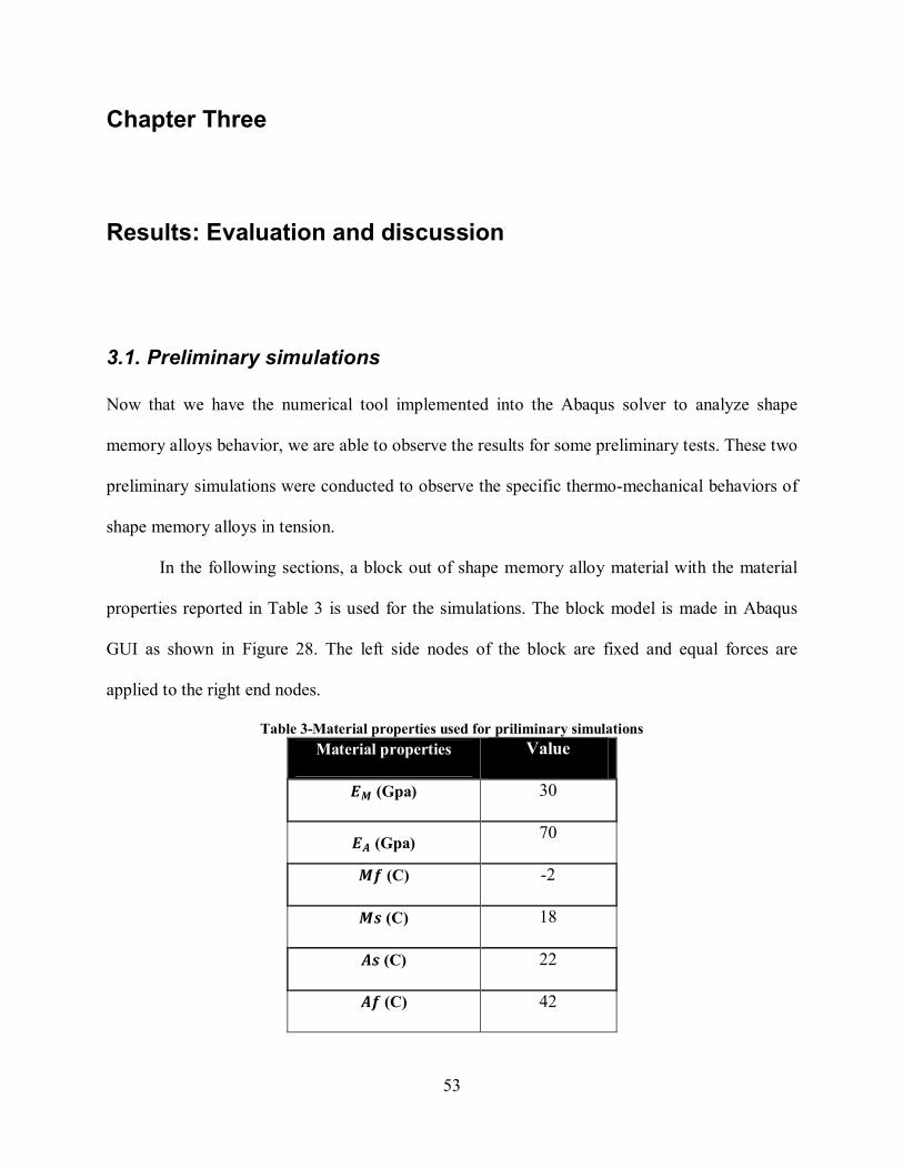
3.1. Preliminary simulations Now that we have the numerical tool implemented into the Abaqus solver to analyze shape

memory alloys behavior, we are able to observe the results for some preliminary tests. These two

preliminary simulations were conducted to observe the specific thermo-mechanical behaviors of

shape memory alloys in tension.

In the following sections, a block out of shape memory alloy material with the material

properties reported in Table 3 is used for the simulations. The block model is made in Abaqus

GUI as shown in Figure 28. The left side nodes of the block are fixed and equal forces are

applied to the right end nodes.

Table 3-Material properties used for priliminary simulations

Material properties Value

�� (Gpa) 30

�� (Gpa) 70

�� (C) -2

�� (C) 18

�� (C) 22

�� (C) 42

54

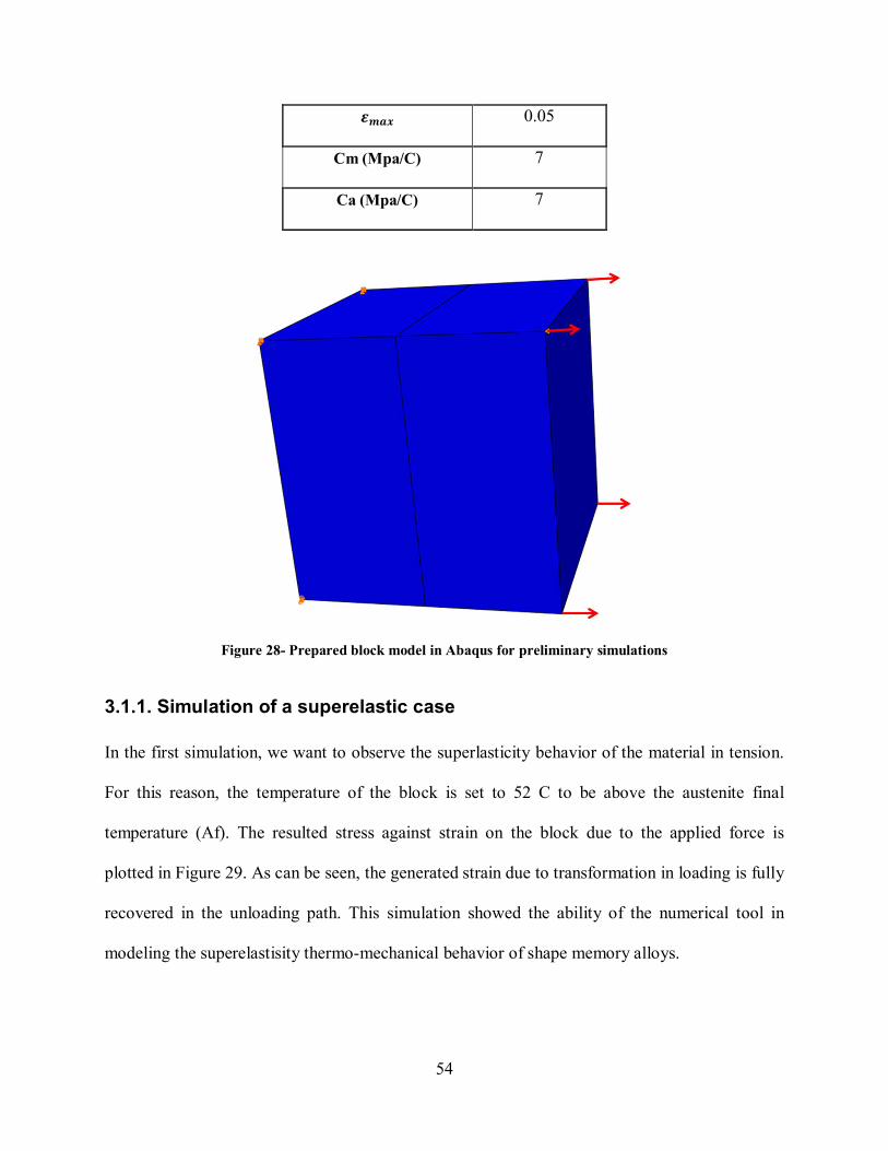
���� 0.05

Cm (Mpa/C) 7

Ca (Mpa/C) 7

Figure 28- Prepared block model in Abaqus for preliminary simulations

3.1.1. Simulation of a superelastic case

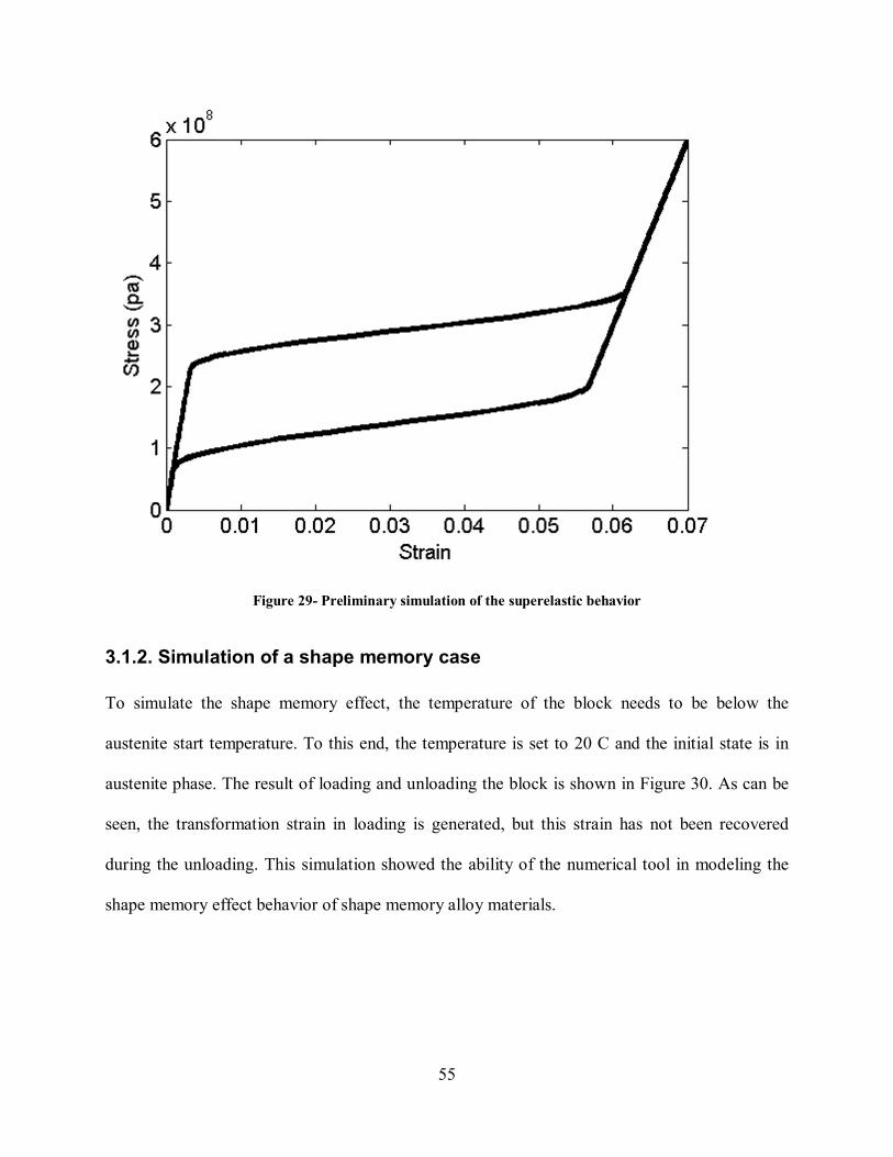
In the first simulation, we want to observe the superlasticity behavior of the material in tension.

For this reason, the temperature of the block is set to 52 C to be above the austenite final

temperature (Af). The resulted stress against strain on the block due to the applied force is

plotted in Figure 29. As can be seen, the generated strain due to transformation in loading is fully

recovered in the unloading path. This simulation showed the ability of the numerical tool in

modeling the superelastisity thermo-mechanical behavior of shape memory alloys.

55

Figure 29- Preliminary simulation of the superelastic behavior

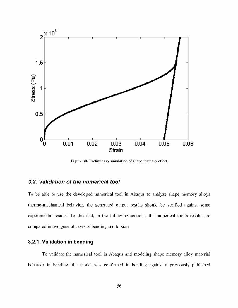
3.1.2. Simulation of a shape memory case

To simulate the shape memory effect, the temperature of the block needs to be below the

austenite start temperature. To this end, the temperature is set to 20 C and the initial state is in

austenite phase. The result of loading and unloading the block is shown in Figure 30. As can be

seen, the transformation strain in loading is generated, but this strain has not been recovered

during the unloading. This simulation showed the ability of the numerical tool in modeling the

shape memory effect behavior of shape memory alloy materials.

56

Figure 30- Preliminary simulation of shape memory effect

3.2. Validation of the numerical tool To be able to use the developed numerical tool in Abaqus to analyze shape memory alloys

thermo-mechanical behavior, the generated output results should be verified against some

experimental results. To this end, in the following sections, the numerical tool’s results are

compared in two general cases of bending and torsion.

3.2.1. Validation in bending

To validate the numerical tool in Abaqus and modeling shape memory alloy material

behavior in bending, the model was confirmed in bending against a previously published

57

experiment. This exercise was conducted to verify the model accuracy. For all simulations

presented, implicit Abaqus solver was utilized.

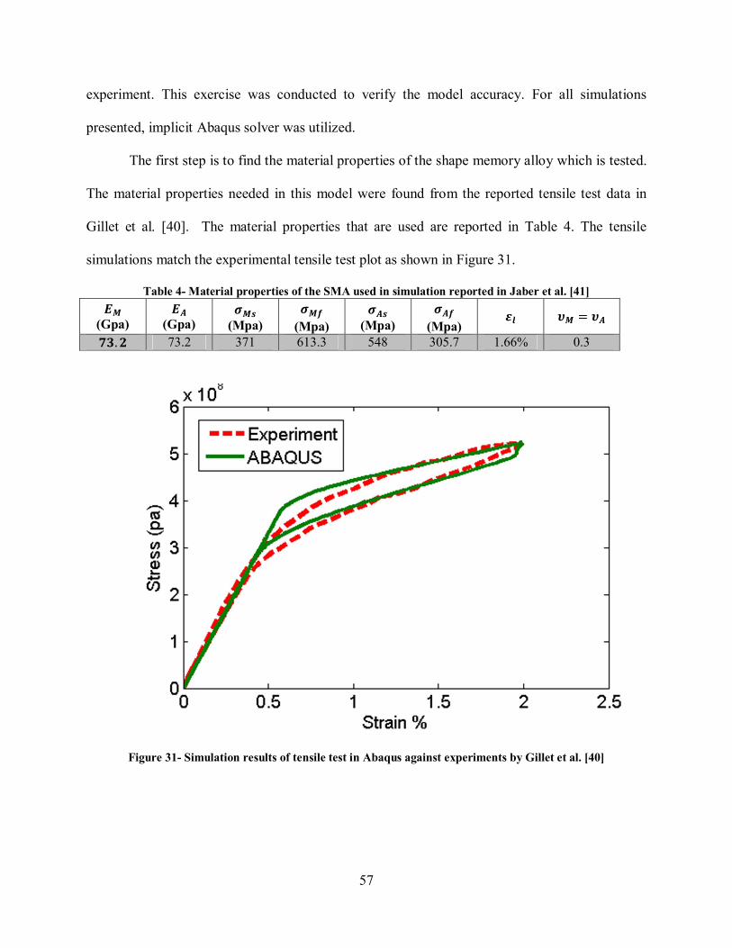
The first step is to find the material properties of the shape memory alloy which is tested.

The material properties needed in this model were found from the reported tensile test data in

Gillet et al. [40]. The material properties that are used are reported in Table 4. The tensile

simulations match the experimental tensile test plot as shown in Figure 31.

Table 4- Material properties of the SMA used in simulation reported in Jaber et al. [41]

�� (Gpa)

�� (Gpa)

��� (Mpa)

���

(Mpa)

��� (Mpa)

���

(Mpa) �� �� = ��

��.� 73.2 371 613.3 548 305.7 1.66% 0.3

Figure 31- Simulation results of tensile test in Abaqus against experiments by Gillet et al. [40]

58

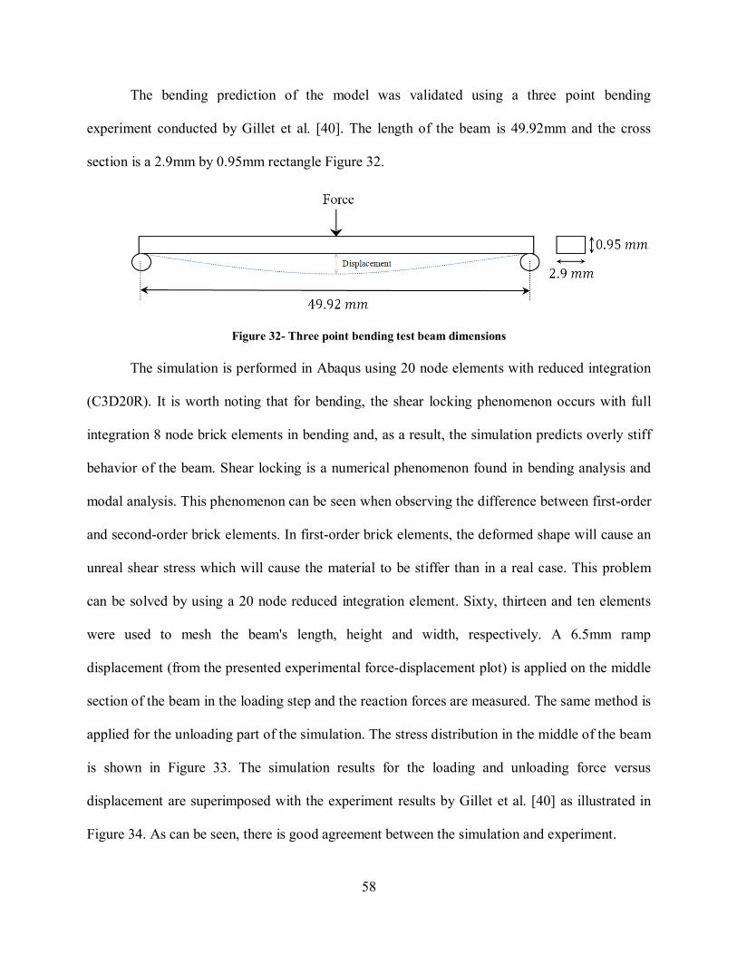
The bending prediction of the model was validated using a three point bending

experiment conducted by Gillet et al. [40]. The length of the beam is 49.92mm and the cross

section is a 2.9mm by 0.95mm rectangle Figure 32.

Figure 32- Three point bending test beam dimensions

The simulation is performed in Abaqus using 20 node elements with reduced integration

(C3D20R). It is worth noting that for bending, the shear locking phenomenon occurs with full

integration 8 node brick elements in bending and, as a result, the simulation predicts overly stiff

behavior of the beam. Shear locking is a numerical phenomenon found in bending analysis and

modal analysis. This phenomenon can be seen when observing the difference between first-order

and second-order brick elements. In first-order brick elements, the deformed shape will cause an

unreal shear stress which will cause the material to be stiffer than in a real case. This problem

can be solved by using a 20 node reduced integration element. Sixty, thirteen and ten elements

were used to mesh the beam's length, height and width, respectively. A 6.5mm ramp

displacement (from the presented experimental force-displacement plot) is applied on the middle

section of the beam in the loading step and the reaction forces are measured. The same method is

applied for the unloading part of the simulation. The stress distribution in the middle of the beam

is shown in Figure 33. The simulation results for the loading and unloading force versus

displacement are superimposed with the experiment results by Gillet et al. [40] as illustrated in

Figure 34. As can be seen, there is good agreement between the simulation and experiment.

59

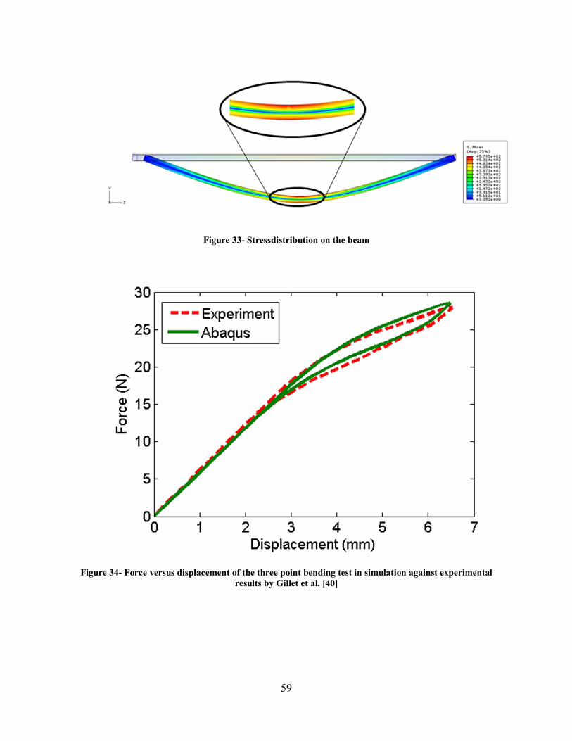
Figure 33- Stressdistribution on the beam

Figure 34- Force versus displacement of the three point bending test in simulation against experimental results by Gillet et al. [40]

60

3.2.2. Validation of the model in torsion

To validate the combination of the Abaqus solver and the developed numerical tool in

modeling shape memory alloy rod in torsion, the results of the simulation were compared to the

experimental data.

To obtain the material properties of the wire samples, three tensile tests were done using

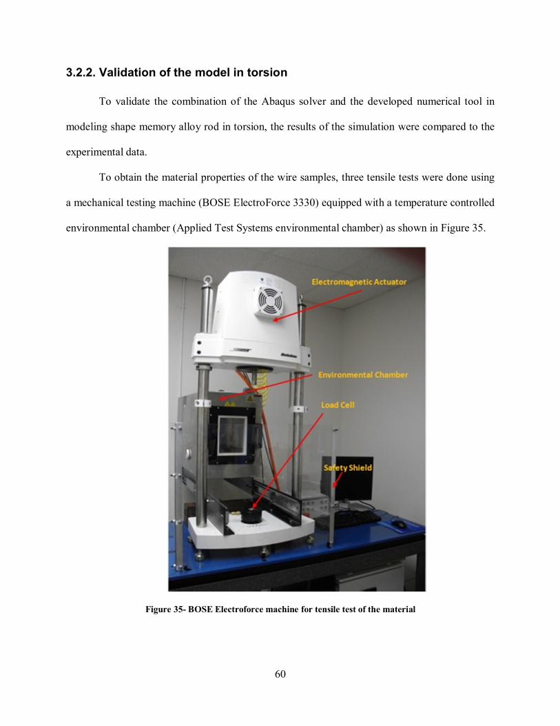
a mechanical testing machine (BOSE ElectroForce 3330) equipped with a temperature controlled

environmental chamber (Applied Test Systems environmental chamber) as shown in Figure 35.

Figure 35- BOSE Electroforce machine for tensile test of the material

61

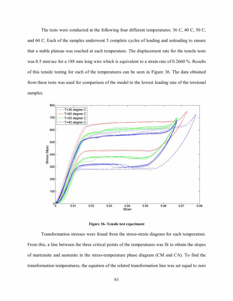
The tests were conducted at the following four different temperatures: 36 C, 40 C, 50 C,

and 60 C. Each of the samples underwent 5 complete cycles of loading and unloading to ensure

that a stable plateau was reached at each temperature. The displacement rate for the tensile tests

was 0.5 mm/sec for a 188 mm long wire which is equivalent to a strain rate of 0.2660 %. Results

of this tensile testing for each of the temperatures can be seen in Figure 36. The data obtained

from these tests was used for comparison of the model to the lowest loading rate of the torsional

samples.

Figure 36- Tensile test experiment

Transformation stresses were found from the stress-strain diagram for each temperature.

From this, a line between the three critical points of the temperatures was fit to obtain the slopes

of martensite and austenite in the stress-temperature phase diagram (CM and CA). To find the

transformation temperatures, the equation of the related transformation line was set equal to zero

62

and the transformation temperatures were found. Young’s Moduli were also calculated from the

stress-strain curves by calculating the slopes of the linear, fully transformed, regions of

martensite and austenite. These material properties are summarized in Table 5.

Table 5- Material properties of the nitinol rod

Symbol Value Unit

�� 40,000 MPa

�� 30,000 MPa

�� -88 oC

�� -33 oC

�� -23 oC

�� -8 oC

�� 5.7 Mpa/ C

�� 8.6 Mpa/ C

�� 0.039 -

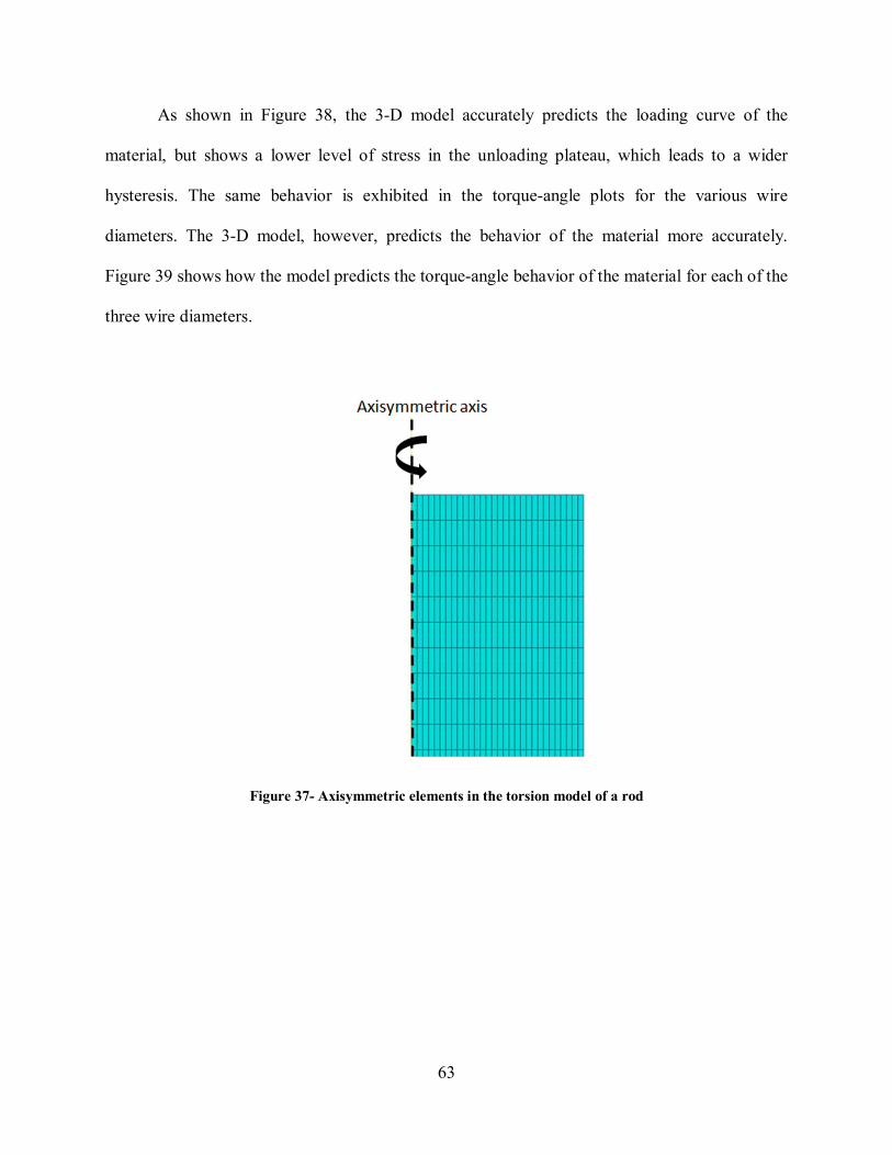
To simulate the behavior in pure torsion an axisymmetric element with a rotational

degree of freedom around its center axis (element CGAX8 from the Abaqus element library) was

used (Figure 37). Similar to the experimental testing, the length of the wires was 0.4 inches

while the diameters were 0.018, 0.020 and .023 inches. The number of elements in the radial

direction from the center to the maximum radius was 30. To get an appropriate aspect ratio, 300

elements were used within the length of the part. The bottom surface of the specimen was held

fixed in the vertical direction. The rotational displacement is applied to the top surface of the

specimen (the maximum applied rotational displacement was chosen from the experimental

results in the rotational displacement). While increasing and decreasing the applied rotation

angle in loading and unloading, the produced reaction torque in the wire was computed by

summing each of the reaction torques at the nodes of the clamped end. All of the simulations

were held at 23 C.

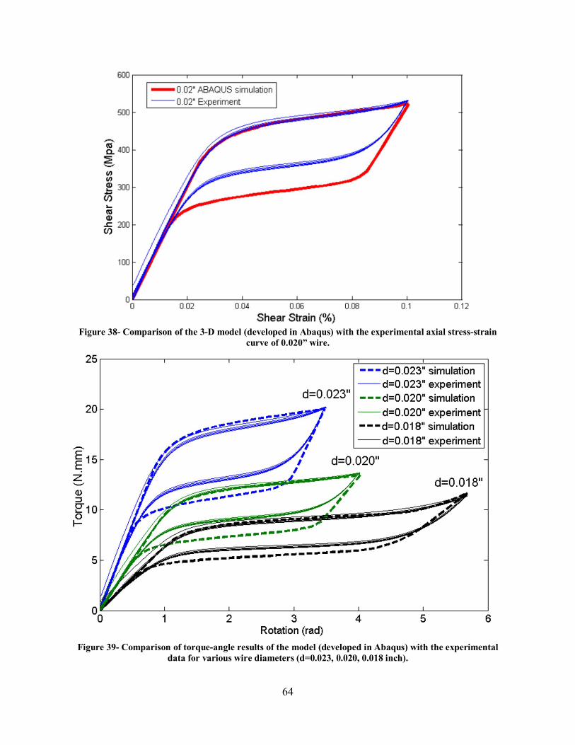
63

As shown in Figure 38, the 3-D model accurately predicts the loading curve of the

material, but shows a lower level of stress in the unloading plateau, which leads to a wider

hysteresis. The same behavior is exhibited in the torque-angle plots for the various wire

diameters. The 3-D model, however, predicts the behavior of the material more accurately.

Figure 39 shows how the model predicts the torque-angle behavior of the material for each of the

three wire diameters.

Figure 37- Axisymmetric elements in the torsion model of a rod

64

Figure 38- Comparison of the 3-D model (developed in Abaqus) with the experimental axial stress-strain

curve of 0.020” wire.

Figure 39- Comparison of torque-angle results of the model (developed in Abaqus) with the experimental

data for various wire diameters (d=0.023, 0.020, 0.018 inch).

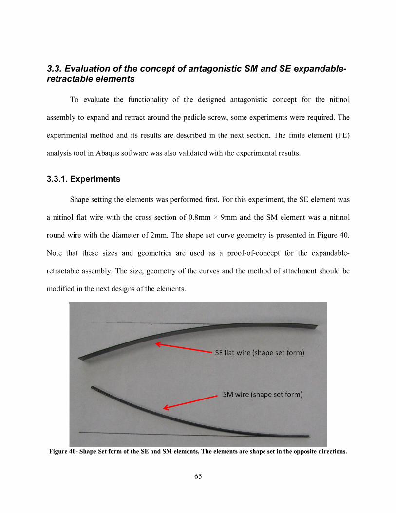
65

3.3. Evaluation of the concept of antagonistic SM and SE expandable-retractable elements

To evaluate the functionality of the designed antagonistic concept for the nitinol

assembly to expand and retract around the pedicle screw, some experiments were required. The

experimental method and its results are described in the next section. The finite element (FE)

analysis tool in Abaqus software was also validated with the experimental results.

3.3.1. Experiments

Shape setting the elements was performed first. For this experiment, the SE element was

a nitinol flat wire with the cross section of 0.8mm × 9mm and the SM element was a nitinol

round wire with the diameter of 2mm. The shape set curve geometry is presented in Figure 40.

Note that these sizes and geometries are used as a proof-of-concept for the expandable-

retractable assembly. The size, geometry of the curves and the method of attachment should be

modified in the next designs of the elements.

Figure 40- Shape Set form of the SE and SM elements. The elements are shape set in the opposite directions.

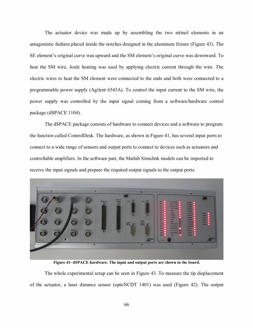
66

The actuator device was made up by assembling the two nitinol elements in an

antagonistic fashion placed inside the notches designed in the aluminum fixture (Figure 43). The

SE element’s original curve was upward and the SM element’s original curve was downward. To

heat the SM wire, Joule heating was used by applying electric current through the wire. The

electric wires to heat the SM element were connected to the ends and both were connected to a

programmable power supply (Agilent 6543A). To control the input current to the SM wire, the

power supply was controlled by the input signal coming from a software/hardware control

package (dSPACE 1104).

The dSPACE package consists of hardware to connect devices and a software to program

the function called ControlDesk. The hardware, as shown in Figure 41, has several input ports to

connect to a wide range of sensors and output ports to connect to devices such as actuators and

controllable amplifiers. In the software part, the Matlab Simulink models can be imported to

receive the input signals and prepare the required output signals to the output ports.

Figure 41- dSPACE hardware. The input and output ports are shown in the board.

The whole experimental setup can be seen in Figure 43. To measure the tip displacement

of the actuator, a laser distance sensor (optoNCDT 1401) was used (Figure 42). The output

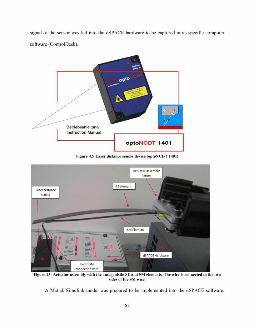
67

signal of the sensor was fed into the dSPACE hardware to be captured in its specific computer

software (ControlDesk).

Figure 42- Laser distance sensor device (optoNCDT 1401)

Figure 43- Actuator assembly with the antagonistic SE and SM elements. The wire is connected to the two

sides of the SM wire.

A Matlab Simulink model was prepared to be implemented into the dSPACE software.

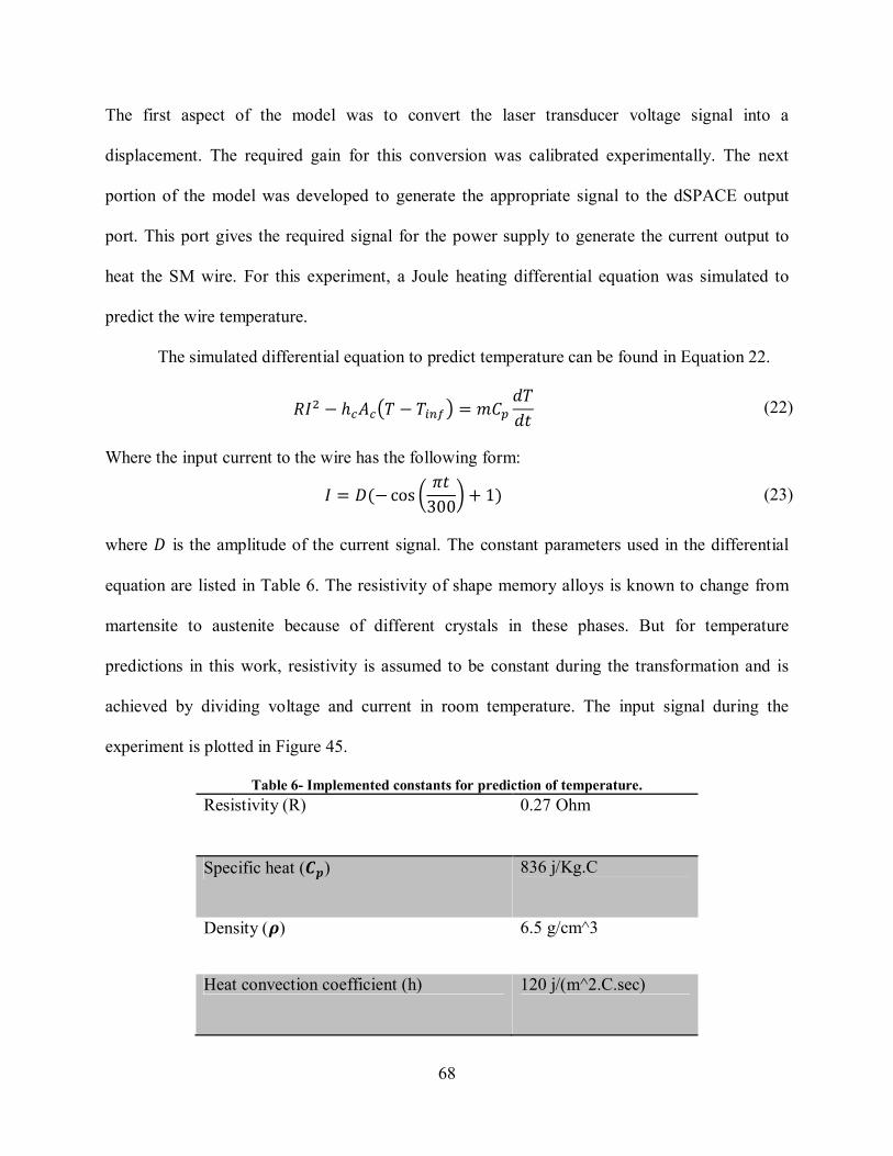
68

The first aspect of the model was to convert the laser transducer voltage signal into a

displacement. The required gain for this conversion was calibrated experimentally. The next

portion of the model was developed to generate the appropriate signal to the dSPACE output

port. This port gives the required signal for the power supply to generate the current output to

heat the SM wire. For this experiment, a Joule heating differential equation was simulated to

predict the wire temperature.

The simulated differential equation to predict temperature can be found in Equation 22.

��� − ℎ����� − ����� = �����

�� (22)

Where the input current to the wire has the following form:

where � is the amplitude of the current signal. The constant parameters used in the differential

equation are listed in Table 6. The resistivity of shape memory alloys is known to change from

martensite to austenite because of different crystals in these phases. But for temperature

predictions in this work, resistivity is assumed to be constant during the transformation and is

achieved by dividing voltage and current in room temperature. The input signal during the

experiment is plotted in Figure 45.

Table 6- Implemented constants for prediction of temperature.

Resistivity (R) 0.27 Ohm

Specific heat (��) 836 j/Kg.C

Density (�) 6.5 g/cm^3

Heat convection coefficient (h) 120 j/(m^2.C.sec)

� = �(−cos ���

300� + 1) (23)

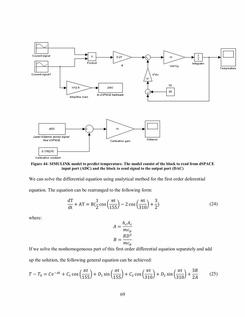
69

Figure 44- SIMULINK model to predict temperature. The model consist of the block to read from dSPACE

input port (ADC) and the block to send signal to the output port (DAC)

We can solve the differential equation using analytical method for the first order deferential

equation. The equation can be rearranged to the following form:

dT

dt+ AT = B(

1

2cos �

πt

155� − 2 cos �

πt

310� +

3

2) (24)

where:

� =ℎ������

� =���

���

If we solve the nonhomogeneous part of this first order differential equation separately and add

up the solution, the following general equation can be achieved:

� − �� = ����� + �� cos �

��

155�+ �� sin �

��

155� + �� cos �

��

310� + �� sin �

��

310� +

3�

2� (25)

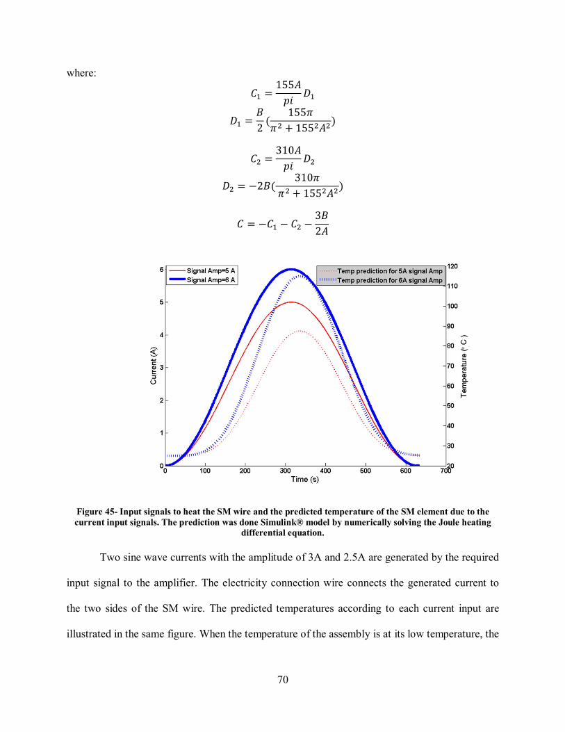
70

where:

�� =155�

����

�� =�

2(

155�

�� + 155���)

�� =310�

����

�� = −2�(310�

�� + 155���)

� = −�� − �� −3�

2�

Figure 45- Input signals to heat the SM wire and the predicted temperature of the SM element due to the current input signals. The prediction was done Simulink® model by numerically solving the Joule heating

differential equation.

Two sine wave currents with the amplitude of 3A and 2.5A are generated by the required

input signal to the amplifier. The electricity connection wire connects the generated current to

the two sides of the SM wire. The predicted temperatures according to each current input are

illustrated in the same figure. When the temperature of the assembly is at its low temperature, the

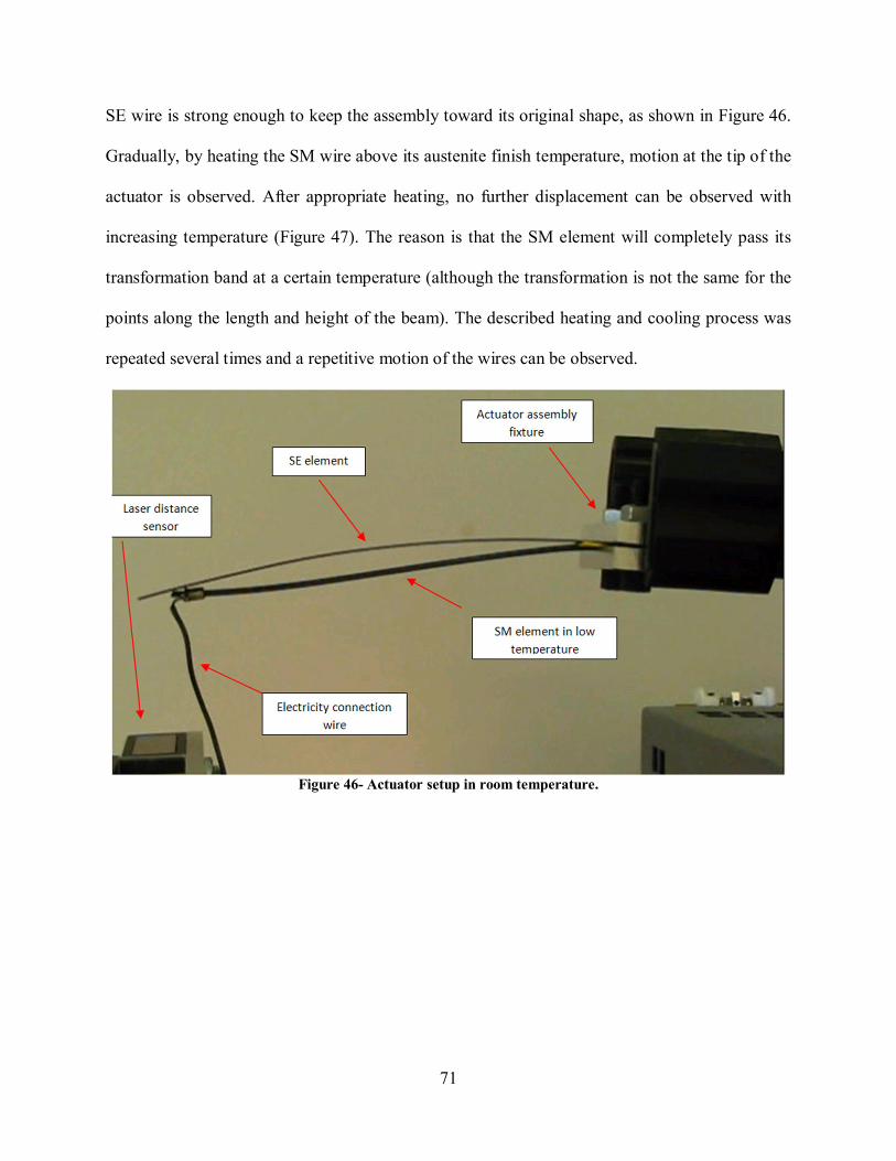
71

SE wire is strong enough to keep the assembly toward its original shape, as shown in Figure 46.

Gradually, by heating the SM wire above its austenite finish temperature, motion at the tip of the

actuator is observed. After appropriate heating, no further displacement can be observed with

increasing temperature (Figure 47). The reason is that the SM element will completely pass its

transformation band at a certain temperature (although the transformation is not the same for the

points along the length and height of the beam). The described heating and cooling process was

repeated several times and a repetitive motion of the wires can be observed.

Figure 46- Actuator setup in room temperature.

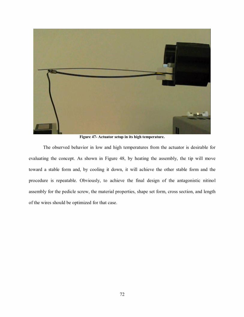
72

Figure 47- Actuator setup in its high temperature.

The observed behavior in low and high temperatures from the actuator is desirable for

evaluating the concept. As shown in Figure 48, by heating the assembly, the tip will move

toward a stable form and, by cooling it down, it will achieve the other stable form and the

procedure is repeatable. Obviously, to achieve the final design of the antagonistic nitinol

assembly for the pedicle screw, the material properties, shape set form, cross section, and length

of the wires should be optimized for that case.

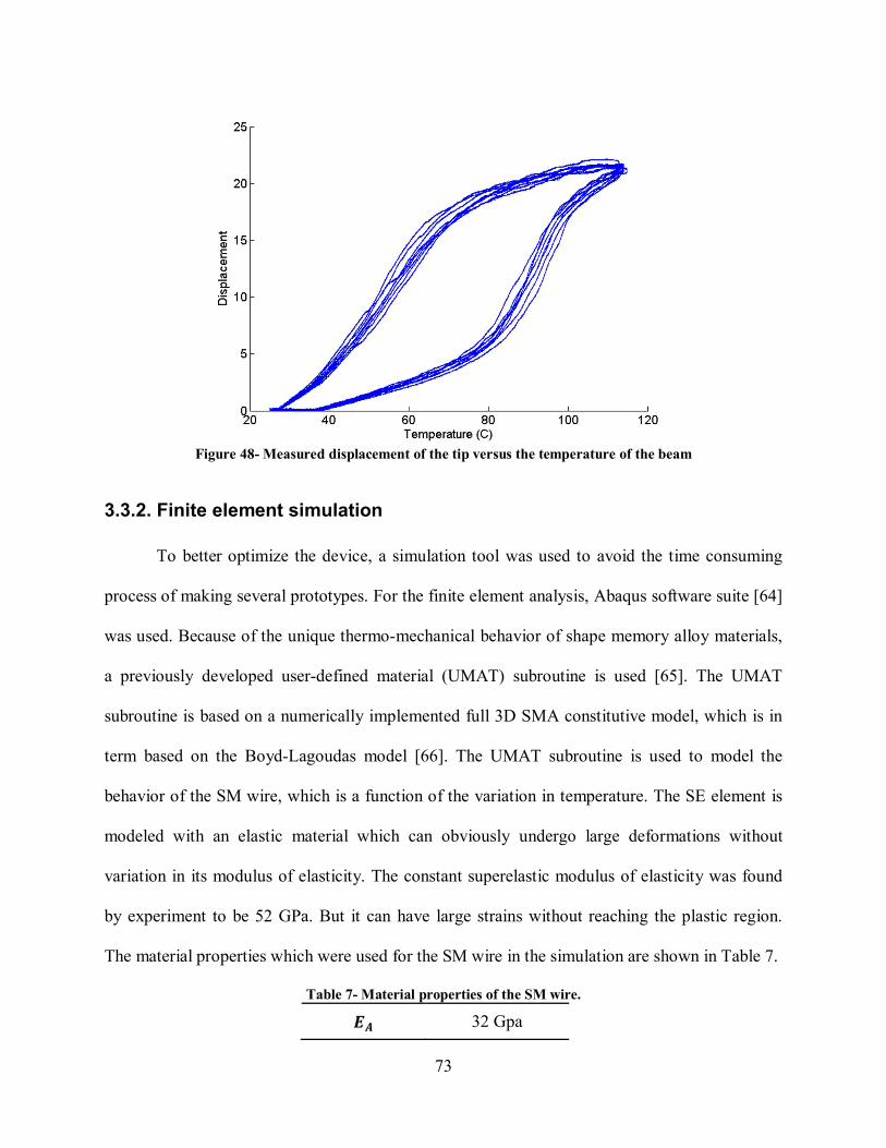
73

Figure 48- Measured displacement of the tip versus the temperature of the beam

3.3.2. Finite element simulation

To better optimize the device, a simulation tool was used to avoid the time consuming

process of making several prototypes. For the finite element analysis, Abaqus software suite [64]

was used. Because of the unique thermo-mechanical behavior of shape memory alloy materials,

a previously developed user-defined material (UMAT) subroutine is used [65]. The UMAT

subroutine is based on a numerically implemented full 3D SMA constitutive model, which is in

term based on the Boyd-Lagoudas model [66]. The UMAT subroutine is used to model the

behavior of the SM wire, which is a function of the variation in temperature. The SE element is

modeled with an elastic material which can obviously undergo large deformations without

variation in its modulus of elasticity. The constant superelastic modulus of elasticity was found

by experiment to be 52 GPa. But it can have large strains without reaching the plastic region.

The material properties which were used for the SM wire in the simulation are shown in Table 7.

Table 7- Material properties of the SM wire.

�� 32 Gpa

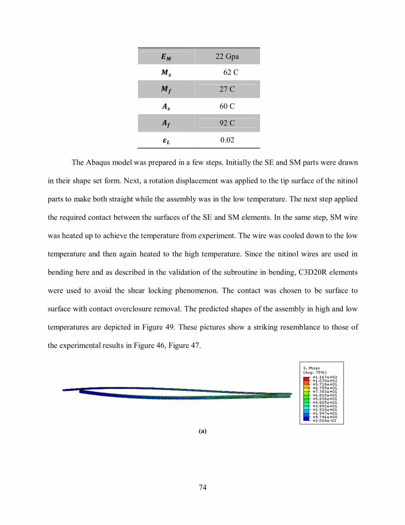
74

�� 22 Gpa

�� 62 C

�� 27 C

�� 60 C

�� 92 C

�� 0.02

The Abaqus model was prepared in a few steps. Initially the SE and SM parts were drawn

in their shape set form. Next, a rotation displacement was applied to the tip surface of the nitinol

parts to make both straight while the assembly was in the low temperature. The next step applied

the required contact between the surfaces of the SE and SM elements. In the same step, SM wire

was heated up to achieve the temperature from experiment. The wire was cooled down to the low

temperature and then again heated to the high temperature. Since the nitinol wires are used in

bending here and as described in the validation of the subroutine in bending, C3D20R elements

were used to avoid the shear locking phenomenon. The contact was chosen to be surface to

surface with contact overclosure removal. The predicted shapes of the assembly in high and low

temperatures are depicted in Figure 49. These pictures show a striking resemblance to those of

the experimental results in Figure 46, Figure 47.

(a)

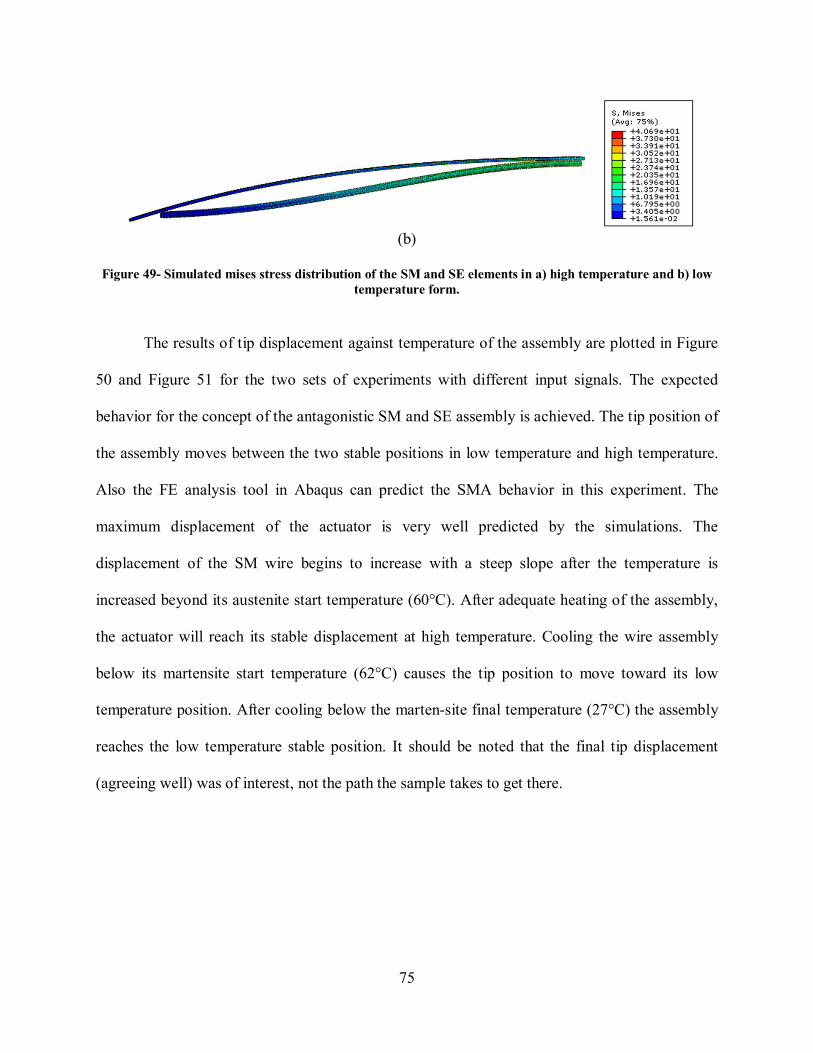
75

(b)

Figure 49- Simulated mises stress distribution of the SM and SE elements in a) high temperature and b) low

temperature form.

The results of tip displacement against temperature of the assembly are plotted in Figure

50 and Figure 51 for the two sets of experiments with different input signals. The expected

behavior for the concept of the antagonistic SM and SE assembly is achieved. The tip position of

the assembly moves between the two stable positions in low temperature and high temperature.

Also the FE analysis tool in Abaqus can predict the SMA behavior in this experiment. The

maximum displacement of the actuator is very well predicted by the simulations. The

displacement of the SM wire begins to increase with a steep slope after the temperature is

increased beyond its austenite start temperature (60°C). After adequate heating of the assembly,

the actuator will reach its stable displacement at high temperature. Cooling the wire assembly

below its martensite start temperature (62°C) causes the tip position to move toward its low

temperature position. After cooling below the marten-site final temperature (27°C) the assembly

reaches the low temperature stable position. It should be noted that the final tip displacement

(agreeing well) was of interest, not the path the sample takes to get there.

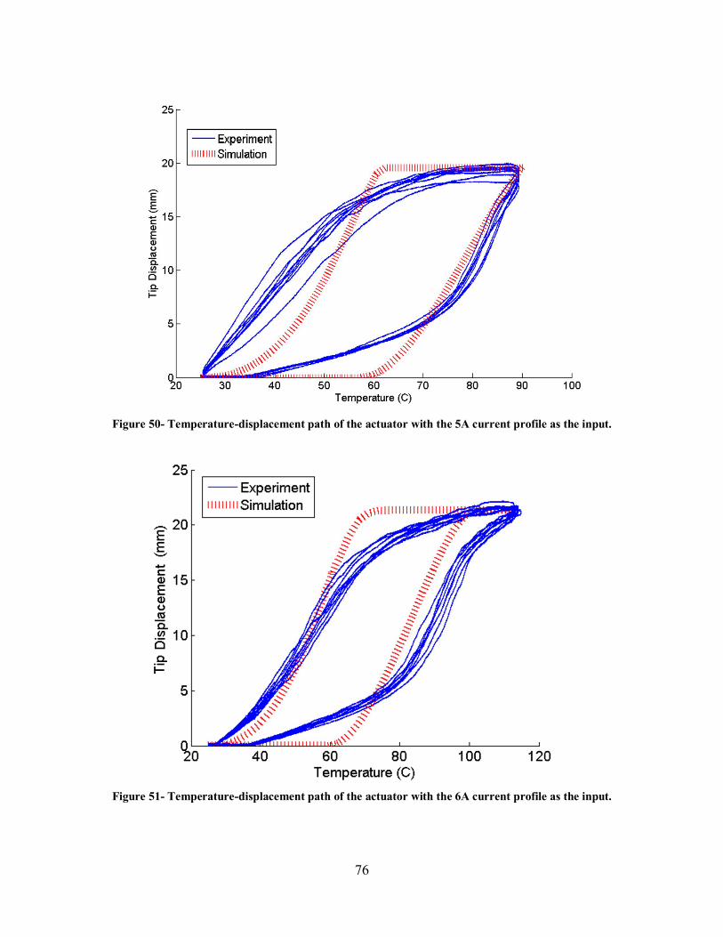
76

Figure 50- Temperature-displacement path of the actuator with the 5A current profile as the input.

Figure 51- Temperature-displacement path of the actuator with the 6A current profile as the input.

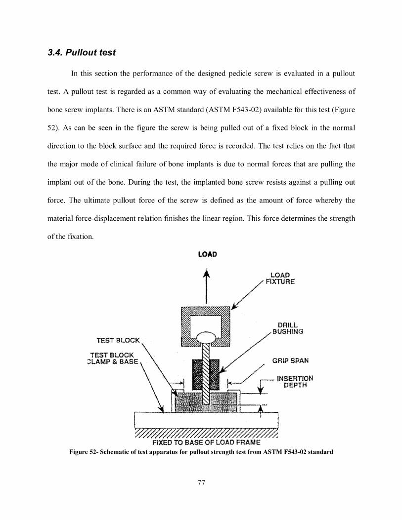
77

3.4. Pullout test

In this section the performance of the designed pedicle screw is evaluated in a pullout

test. A pullout test is regarded as a common way of evaluating the mechanical effectiveness of

bone screw implants. There is an ASTM standard (ASTM F543-02) available for this test (Figure

52). As can be seen in the figure the screw is being pulled out of a fixed block in the normal

direction to the block surface and the required force is recorded. The test relies on the fact that

the major mode of clinical failure of bone implants is due to normal forces that are pulling the

implant out of the bone. During the test, the implanted bone screw resists against a pulling out

force. The ultimate pullout force of the screw is defined as the amount of force whereby the

material force-displacement relation finishes the linear region. This force determines the strength

of the fixation.

Figure 52- Schematic of test apparatus for pullout strength test from ASTM F543-02 standard

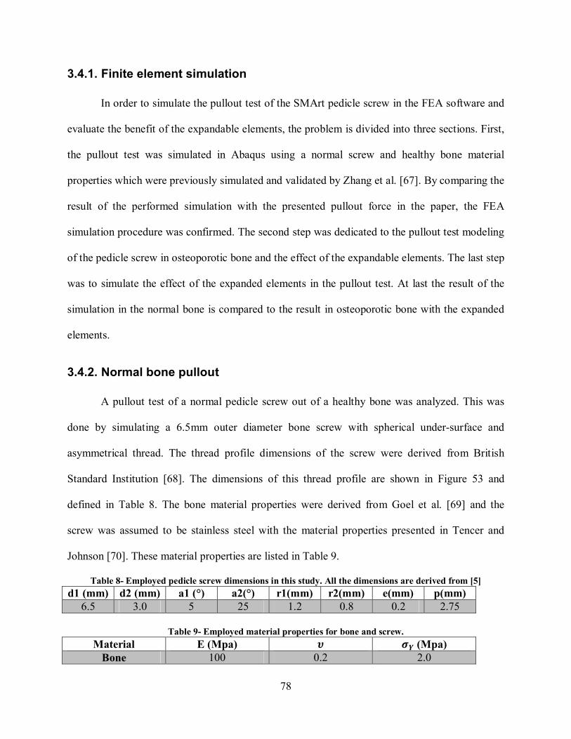
78

3.4.1. Finite element simulation

In order to simulate the pullout test of the SMArt pedicle screw in the FEA software and

evaluate the benefit of the expandable elements, the problem is divided into three sections. First,

the pullout test was simulated in Abaqus using a normal screw and healthy bone material

properties which were previously simulated and validated by Zhang et al. [67]. By comparing the

result of the performed simulation with the presented pullout force in the paper, the FEA

simulation procedure was confirmed. The second step was dedicated to the pullout test modeling

of the pedicle screw in osteoporotic bone and the effect of the expandable elements. The last step

was to simulate the effect of the expanded elements in the pullout test. At last the result of the

simulation in the normal bone is compared to the result in osteoporotic bone with the expanded

elements.

3.4.2. Normal bone pullout

A pullout test of a normal pedicle screw out of a healthy bone was analyzed. This was

done by simulating a 6.5mm outer diameter bone screw with spherical under-surface and

asymmetrical thread. The thread profile dimensions of the screw were derived from British

Standard Institution [68]. The dimensions of this thread profile are shown in Figure 53 and

defined in Table 8. The bone material properties were derived from Goel et al. [69] and the

screw was assumed to be stainless steel with the material properties presented in Tencer and

Johnson [70]. These material properties are listed in Table 9.

Table 8- Employed pedicle screw dimensions in this study. All the dimensions are derived from [5]

d1 (mm) d2 (mm) a1 (°) a2(°) r1(mm) r2(mm) e(mm) p(mm) 6.5 3.0 5 25 1.2 0.8 0.2 2.75

Table 9- Employed material properties for bone and screw.

Material E (Mpa) � �� (Mpa) Bone 100 0.2 2.0

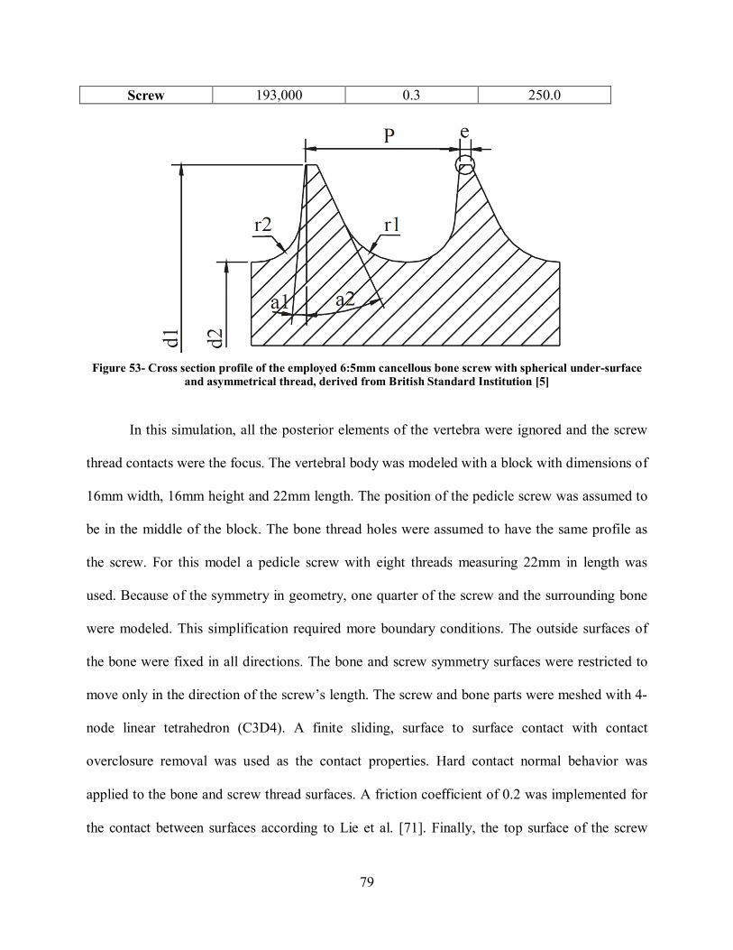
79

Screw 193,000 0.3 250.0

Figure 53- Cross section profile of the employed 6:5mm cancellous bone screw with spherical under-surface

and asymmetrical thread, derived from British Standard Institution [5]

In this simulation, all the posterior elements of the vertebra were ignored and the screw

thread contacts were the focus. The vertebral body was modeled with a block with dimensions of

16mm width, 16mm height and 22mm length. The position of the pedicle screw was assumed to

be in the middle of the block. The bone thread holes were assumed to have the same profile as

the screw. For this model a pedicle screw with eight threads measuring 22mm in length was

used. Because of the symmetry in geometry, one quarter of the screw and the surrounding bone

were modeled. This simplification required more boundary conditions. The outside surfaces of

the bone were fixed in all directions. The bone and screw symmetry surfaces were restricted to

move only in the direction of the screw’s length. The screw and bone parts were meshed with 4-

node linear tetrahedron (C3D4). A finite sliding, surface to surface contact with contact

overclosure removal was used as the contact properties. Hard contact normal behavior was

applied to the bone and screw thread surfaces. A friction coefficient of 0.2 was implemented for

the contact between surfaces according to Lie et al. [71]. Finally, the top surface of the screw

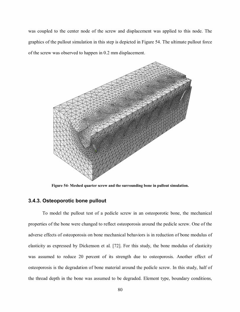
80

was coupled to the center node of the screw and displacement was applied to this node. The

graphics of the pullout simulation in this step is depicted in Figure 54. The ultimate pullout force

of the screw was observed to happen in 0.2 mm displacement.

Figure 54- Meshed quarter screw and the surrounding bone in pullout simulation.

3.4.3. Osteoporotic bone pullout

To model the pullout test of a pedicle screw in an osteoporotic bone, the mechanical

properties of the bone were changed to reflect osteoporosis around the pedicle screw. One of the

adverse effects of osteoporosis on bone mechanical behaviors is in reduction of bone modulus of

elasticity as expressed by Dickenson et al. [72]. For this study, the bone modulus of elasticity

was assumed to reduce 20 percent of its strength due to osteoporosis. Another effect of

osteoporosis is the degradation of bone material around the pedicle screw. In this study, half of

the thread depth in the bone was assumed to be degraded. Element type, boundary conditions,

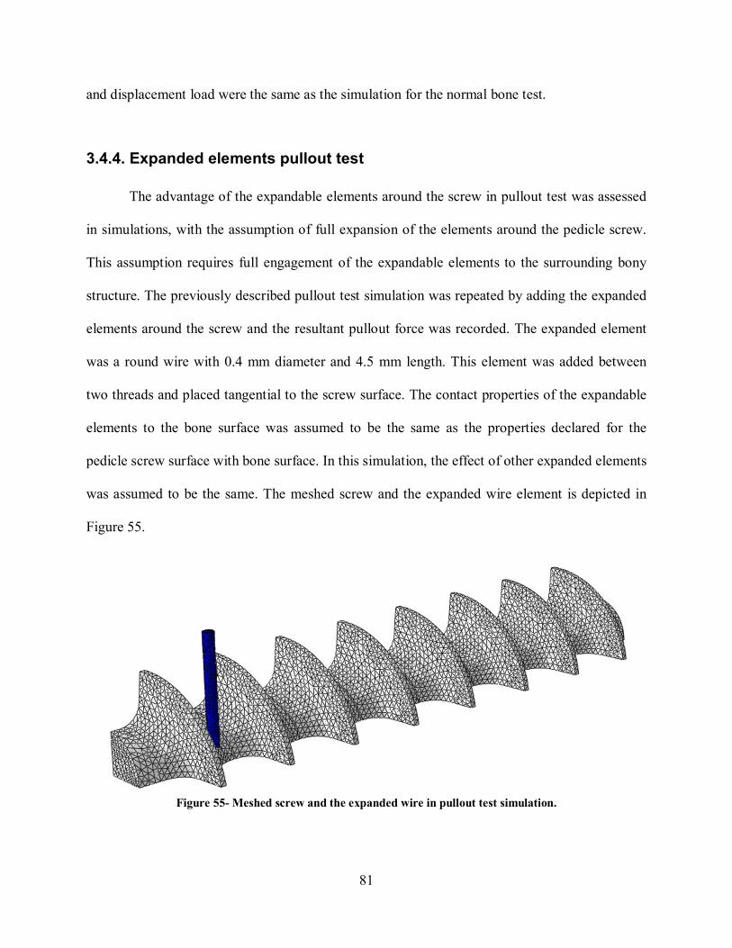
81

and displacement load were the same as the simulation for the normal bone test.

3.4.4. Expanded elements pullout test

The advantage of the expandable elements around the screw in pullout test was assessed

in simulations, with the assumption of full expansion of the elements around the pedicle screw.

This assumption requires full engagement of the expandable elements to the surrounding bony

structure. The previously described pullout test simulation was repeated by adding the expanded

elements around the screw and the resultant pullout force was recorded. The expanded element

was a round wire with 0.4 mm diameter and 4.5 mm length. This element was added between

two threads and placed tangential to the screw surface. The contact properties of the expandable

elements to the bone surface was assumed to be the same as the properties declared for the

pedicle screw surface with bone surface. In this simulation, the effect of other expanded elements

was assumed to be the same. The meshed screw and the expanded wire element is depicted in

Figure 55.

Figure 55- Meshed screw and the expanded wire in pullout test simulation.

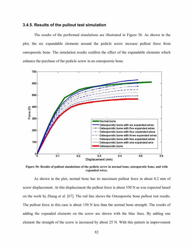
82

3.4.5. Results of the pullout test simulation

The results of the performed simulations are illustrated in Figure 56. As shown in the

plot, the six expandable elements around the pedicle screw increase pullout force from

osteoporotic bone. The simulation results confirm the effect of the expandable elements which

enhance the purchase of the pedicle screw in an osteoporotic bone.

Figure 56- Results of pullout simulations of the pedicle screw in normal bone, osteoporotic bone, and with

expanded wires.

As shown in the plot, normal bone has its maximum pullout force in about 0.2 mm of

screw displacement. At this displacement the pullout force is about 550 N as was expected based

on the work by Zhang et al. [67]. The red line shows the Osteoporotic bone pullout test results.

The pullout force in this case is about 150 N less than the normal bone strength. The results of

adding the expanded elements on the screw are shown with the blue lines. By adding one

element the strength of the screw is increased by about 25 N. With this pattern in improvement

83

of the screw pullout force, the performance of the pedicle screw will reach to the normal

behavior with 6 expanded elements around the screw. The results of simulations show that the

purchase of the pedicle screw in the bone is enhanced by the nitinol expanded elements.

84

Chapter Four

Conclusion and Future Work

4.1. Conclusion

Shape memory alloys are a unique kind of alloys which show a specific thermo-

mechanical behavior. They have the ability to return to a certain predefined shape upon heating

after deformation. The second specific property is the ability to tolerate large deformations

without undergoing the plastic region. These specific properties along with the biocompatibility

of nitinol are the reasons that this alloy has been used in recent years for biomedical devices

applications

To better design and analyze the nitinol devices which are used in biomedical

applications, a simulation tool is required. To this end, the constitutive modeling of the thermo-

mechanical behavior of the shape memory alloys has been implemented into the Abaqus UMAT

subroutine and works in combination with the Abaqus finite element solver.

A novel pedicle screw design which has been proposed previously is analyzed in this

study. The unique part of the design was the assemblies which were placed on the pedicle screws

shaft. The assemblies were made out of nitinol material which brought the capability of

expanding and retracting (in certain temperatures) to the screw. The functionality of the

described assembly was evaluated by making a prototype in larger scale and performing

experiments. The result of the tip displacement of the assembly was recorded and reported as the

85

function of temperature variation of the nitinol beam. The FEA modeling of SMA material

thermo-mechanical behavior in Abaqus was also conducted and verified by comparing the results

with the experimental ones. Pullout test as the standard method of evaluating the pedicle screws

was also modeled in Abaqus as the FEA modeling software. In the modeling, the pullout test

results of a regular screw were compared to the enhanced screw with expandable elements. In

both experiment and modeling, the expandable screw showed much higher pullout force than a

regular screw.

4.2. Future Work This work can be continued in different aspects. First, the numerical thermo-mechanical

modeling of the shape memory alloy material in Abaqus can be further improved. Shape memory

alloys are known to have different behaviors in different rates of loading the material. The

numerical UMAT subroutine can be developed to capture the rate dependency of the shape

memory alloy behaviors based on the developed equations in literature. This capability enables

the numerical tool to be able to be used in variety of applications. Other than that, the ability of

modeling different material properties in one simulation which is not possible in the current

version of the UMAT subroutine can be added.

Moreover, now that we have the capability of finite element simulating of the thermo-

mechanical behavior of the devices made out of nitinol in Abaqus, there is the possibility to

modify, analyze and prototype other designs for the pedicle screw to better mitigate osteoporosis

effect. In the future designs, the possibility of easy production of the device should be better

considered. In the design procedure different capabilities in producing nitinol geometries should

be considered.

86

Additionally, the pullout test finite element simulation can be improved in more realistic

way and be compared to the experiments. The procedure of failure of the bone in the pullout test

of pedicle screw should be studied in more medical aspects details and be considered in the

modeling. After the production of a SMArt pedicle screw the pullout tests in a bone material can

be performed and be compared to the result of a regular screw pullout test.

87

Works Cited

[1] Lagoudas, D. C., 2008. Shape memory alloys: modeling and engineering applications.

Springer

[2] Bekker, A., Brinson, L. C., 1998. Phase diagram based description of the hysteresis

behavior of shape memory alloys. Acta Materialia, Volume 46, Issue 10

[3] Brinson, L. C. “One-Dimensional Constitutive Behavior of Shape Memory Alloys:

Thermomechanical Derivation with Non-Constant Material Functions and Redefined Martensite

Internal Variabl” Journal of intelligent material systems and structures, Vol. 4 no. 2, 1993

[4] D. J. Hartl, D C Lagoudas, F T Calkins and J H Mabe, Use of a Ni60Ti shape memory

alloy for active jet engine chevron application: I. Thermo-mechanical characterization”, Volume

19, No. 1, 2010

[5] D. J. Hartl, Modeling of shape memory alloys considering rate-independent and rate-

dependent irrecoverable strains”, Ph.D thesis, University of Texas A&M \

[6] T. Duerig, A. Pelton, D. Stockel, “An overview of nitinol medical applications”,

Materials Science and Engineering A273–275 (1999) 149–160

[7] Holton, Walsh., “Comparative MRI Compatibility of 316L Stainless Steel Alloy and

Nickel-Titanium Alloy Stents”, Journal of Cardiovascular Magnetic Resonance, 2002, (4)4: 423-

430.

[8] Liu X., Wang Y., Yang D., and Qi M., ―The effect of ageing treatment on shape-setting

and superelasticity of a nitinol stent‖, Materials Characterization, 2008, 59.

[9] http://en.wikipedia.org/wiki/Stent

88

[10] J.P. O’Leary, J.E. Nicholson, R.F. Gatturna, in: T.W. Duerig, K.N. Melton, D. Stockel,

C.M. Waguian (Eds.), Engineering Aspects of Shape Memory Alloys, Butterworth-Heinemann,

Boston, 1990, p. 477.

[11] http://www.cts.usc.edu/zglossary-stent.html

[12] H. Sakamoto et al., US Patent 4 925 445, 1990.

[13] C. Trepanier, et al., Mat. Res. Symp. Proc. 459 (1997) 363.

[14] A. Trigwell, G. Selvaduray, in: A. Pelton, D. Hodgson, R. Russel, T. Duerig (Eds.),

Proceedings of the 2nd International Conference on Shape Memory and Superplastic

Technologies, SMST-97, SMST Proceedings, Pacific Grove, CA, 1997, p. 387.

[15] T.M. Chan et al, Surf. Interf. Anal. 15 (1990) 349.

[16] J. Lausmaa, et al., Mat. Res. Soc. Symp. Proc. 55 (1986) 351.

[17] J.P. Espinos, Surf. Sci. 295 (1993) 420.

[18] Inceoglu S., ―Failure of pedicle screw-bone interface: biomechanics of pedicle screw

insertion and pullout‖, PhD dissertation 2004, Cleveland State University.

[19] http://en.wikipedia.org/wiki/Cortical_bone

[20] Gaines, R. W., 2000. The use of pedicle-screw internal fixation for the operative

treatment of spinal disorder. Journal of Bone and Joint Surgery.

[21] http://www.back.com/anatomy-lumbar.html

[22] Santoni, B. G., Hynes, R. A., McGilvray, K. C., Rodriguez-Canessa, G., Lyons, A. S.,

Henson, M. A. W., Womack, W. J., Puttlitz, C. M., 2008. Cortical bone trajectory for lumbar

pedicle screws. The Spine Journal 9, 366–373.

[23] http://www.thebackcenter.net/pedicle-screws-rods.html

[24] http://www.medscape.com/viewarticle/448311_2

89

[25] Hu, S. S., 1997. Internal fixation in the osteoporotic spine. Spine 22.

[26] Inceoglu, S., 2004. Failure of pedicle screw-bone interface: biomechanics of pedicle

screw insertion and pullout. Ph.D. thesis, Cleveland State University.

[27] http://www.nof.org/osteoporosis/diseasefacts.htm [28] Shigeru S., Shiba R., et al, ”An experimental study on transpedicular screw fixation in

relation to osteoporosis of the lumbar spine”., Spine 1991, 16(11):1335-41.

[29] Hasegawa K., Takahashi H.E., et al., “An Experimental Study of a Combination Method

Using a Pedicle Screw and Laminar Hook for the Osteoporotic Spine, Spine, 1997, 22(9):958-

962.

[30] http://www.mayoclinic.com/health/medical/IM03584

[31] Majid Tabesh, “Finite Element Analysis of Shape Memory Alloy Biomedical Devices,

Ms. Thesis, The University of Toledo, 2010

[32] Smith, R. C, “Smart material systems: model development”, SIAM, 2005

[33] Huo, Y., “A mathematical model for the hysteresis in shape memory alloys”, Continuum

Mechanics and Thermodynamics, 1989, 1(4): 283-303.

[34] Popov, P., and Lagoudas, D.C., “A 3-D constitutive model for shape memory alloys

incorporating pseudoelasticity and detwinning of self-accommodated martensite”, International

Journal of Plasticity, 2007, 23(10-11): 1679-1720.

[35] Tanaka, K., and Nagaki, S., “A thermomechanical description of materials with internal

variables in the process of phase transitions”, Archive of Applied Mechanics (Ingenieur Archiv),

1982, 51 (5): 287-299.

90

[36] Liang, C., and Rogers, C.A., “One-dimensional thermomechanical constitutive relations

for shape memory materials”, Journal of Intelligent Material Systems and Structures, 1990, 1(2):

207-234.

[37] Brinson, L. C., “One-dimensional constitutive behaviour of shape memory alloys:

thermomechanical derivation with non-constant material functions and redefined martensite

internal variable.” journal of intelligent material systems and structures, 1993, Vol. 4.

[38] Brinson, L. C., and Huang, M., “Simplifications and comparisons of shape memory alloy

constitutive models”, Journal of Intelligent Material Systems and Structures, 1996, 7 (1): 108-

114.

[39] Gao, X., Qiao, R., and Brinson, L.C., “Phase diagram kinetics for shape memory alloys: a

robust finite element implementation”, Smart Materials and Structures, 2007, 16 (6): 2102-2115.

[40] Y. Gillet, E. Patoor, and M. Berveiller.” Structure calculations applied to shape memory

alloys”, Journal De Physique IV, 5, 1995.

[41] M. B. Jaber, H. Smaoui, and P. Terriault. Finite element analysis of a shape memory

alloy three-dimensional beam based on a finite strain description. Smart Materials and

Structures, 17, 2008.

[42] D.J. Hartl, D. C. Lagoudas, F. T. Calkins, and J. H. Mabe. Use of a ni60ti shape memory

alloy for active jet engine chevron application: i. thermomechanical characterization. Smart

Material and Structures, 19, 2010.

[43] D.J. Hartl, D. C. Lagoudas, F. T. Calkins, and J. H. Mabe. Use of a ni60ti shape memory

alloy for active jet engine chevron application: ii. experimentally validated numerical analysis.

Smart Material and Structures, 19, 2010.

91

[44] M. Tabesh and M. Elahinia. Modeling and optimization of shape memory-superelastic

antagonistic beam assembly. In Active and Passive Smart Structures and Integrated Systems, San

Diego, CA. SPIE, March 2010.

[45] T. Mineta, T. Mitsui, Y. Watanabe, S. Kobayashi, Y. Haga, and M. Esashi. An active

guide wire with shape memory alloy bending actuator fabricated by room temperature process.

Sensors and Actuators, 97:632{637, 2002.

[46] A. Zbiciak. Dynamic analysis of pseudoelastic sma beam. International Journal of

Mechanical Sciences, 52:56{64, 2010.

[47] R. Mirzaeifar, R. DesRoches, and A. Yavari. Exact solutions for pure torsion of shape

memory alloy circular bars. Mechanics of Materials, 42:797{806, December 2009.

[48] T. Atanackovic and M. Achenbach. Moment-curvature relations for a pseudoelastic

beam. Continuum Mech. Thermodyn., 73-80, 1989.

[49] Ferdinando Auricchio. A superelastic shape-memory-alloy beam model. Journal of

Inteligent Materials and Structures, 8:489{501, 1997.

[50] Kikuaki Tanaka, “A thermomechanical sketch of shape memory effect: one-dimensional

tensile behavior”, Res Mechanica, Volume: 2, Issue: 3 (1986)

[51] Abaqus, 2009. Analysis User's Manual. Dassault Systemes of America Corp., 389

Woodlands Hills, CA.

[52] Qidwai M. A.. and Lagoudas D. C., “Numerical implementation of shape memory alloy

thermomechanical constitutive model using return mapping algorithms”, International Journal

for Numerical Methods in engineering, 47:1123-1168, 2000

[53] Cook S.D., Salkeld S.L., et al., “Biomechanical study of pedicle screw fixation in

severely osteoporotic bone‖, The Spine Journal, 2004, 4: 402–408.

92

[54] Jacob A.T., Ingalhalikar A.V., et al., “Biomechanical comparison of single- and dual-lead

pedicle screws in cadaveric spine Laboratory investigation., Journal of Neurosurgery: Spine, Jan

2008, 8(1): 52-57.

[55] Chapman, J. R., Harrington, R. M., Lee, K. M., Anderson, P. A., Tencer, A. F.,

Kowalski, D., 1996. Factors a ecting the pullout strength of cancellous bone screws. Journal of

Biomechanical Engineering 118 (3).

[56] Battula, S., Schoenfeld, A. J., Sahai, V., Vrabec, G., Tank, J., Nju, G., 2008. The effect of

pilot hole size on the insertion torque and pullout strength of self-tapping cortical bone screws in

osteoporotic bone. Journal of Trauma-Injury Infection & Critical Care 64, 990–995.

[57] Moore, D. C., Maitra, R. S., Farjo, L. A., P, G. G., Goldstein, S. A., 1997. Restoration of

pedicle screw fixation with an in-situ setting calcium phosphate cement. Spine 22 (15).

[58] Cook, S. D., Salkeld, S. L., Stanley, T., Faciane, A., Miller, S. D., 2004. Biomechanical

study of pedicle screw fixation in severely osteoporotic bone. The Spine Journal 4 (4).

[59] Moore, D. C., Maitra, R. S., Farjo, L. A., Graziano, G. P., Goldstein, S. A., 2004. Pedicle

screw motion in the osteoporotic spine after augmentation with laminar hooks, sublaminar wires,

or calcium phosphate cement: A comparative analysis. Spine 29.

[60] Hasegawa, T., Inufusa, A., Mikawa, Y., T, An, H. S., 2005. Hydroxyapatite-coating

of pedicle screws improves resistance against pull-out force in the osteoporotic canine lumbar

spine model: a pilot study. The Spine Journal 5 (3).

[61] McKoy, B. E., An, Y. H., 2001. An expandable anchor for fixation in osteoporotic bone.

Journal of Orthopaedic Research 19 (4).

93

[62] Cook, S. D., Barbera, J., Rubi, M., Salkeld, S. L., Whitecloud, T. S., 2001. Lumbosacral

fixation using expandable pedicle screws: an alternative in reoperation and osteoporosis. The

Spine Journal 1 (2).

[63] Kotenko, M. V., Kopyssova, V. A., Razdorsky, V. V., Kishkarev, V. V., 2008. Shape-

memory dental quadriradical implants for single-stage immediate implantation and undelayed

dental prosthetics. Biomedical Engineering 42 (3).

[64] Abaqus, 2009. Analysis User’s Manual. Dassault Systemes of America Corp.,

Woodlands Hills, CA. 0

[65] Qidwai, M. A., Lagoudas, D. C., 2000. Numerical implementation of a shape memory

alloy thermomechanical constitutive model using return mapping algorithms. International

Journal for Numerical Methods in Engineering 47 (6).

[66] Boyd, J. G., Lagoudas, D. C., 1996. A thermodynamical constitutive model for shape

memory materials. part i. the monolithic shape memory alloy. International Journal of Plasticity

12 (6).

[67] Zhang, Q. H., Tan [67], S. H., Chou, S. M., 2004, “Investigation of fixation screw pull-out

strength on human spine”, Journal of Biomechanics 37

[68] British Standards Institution, 1991. Implants for Osteosynthesis. Part 5, Bone Screws and

Auxiliary Equipment. British Standards Institution, London (Section 5.3, Specification for the

dimensions of screws having hexagonal drive connection, spherical under surfaces and

asymmetrical thread).

[69] Goel, V. K., Kim, Y. E., Lim, T., Weinstein, J. N., 1998. An analytical investigation of

the mechanics of spinal instrumentation. Spine 13 (9).

94

[70] Tencer, A., Johnson, K., 1994. Biomechanics in orthopedic trauma: Bone fracture and

fixation. M. Dunitz (London and Philadelphia).

[71] Liu, C.L., Chen, H. H., Cheng, C. K., Kao, H. C., Lo, W. H., “Biomechanical evaluation

of a new anterior spinal implant”, Journal of Clinical Biomechanics, Volume 13 (1), Sep. 1998

[72] Dickenson, R. P., Hutton, E. C., Stott, J. R., 1981. The mechanical properties of bone in

osteoporosis. Journal of Bone and Joint Surgery-British Volume 63 (2)