A Thesis entitled Optimal Path Planning and Control of ...

A Thesis

entitled

Optimal Path Planning and Control of Quadrotor Unmanned Aerial

Vehicle for Area Coverage

by

Jiankun Fan

Submitted to the Graduate Faculty as partial fulfillment of the requirements for the

Master of Science Degree in Mechanical Engineering

Dr. Manish Kumar, Committee Chair

Dr. Mohammad Elahinia, Committee Member

Dr. Mehdi Pourazady, Committee Member

Dr. Patricia Komuniecki, Dean

College of Graduate Studies

The University of Toledo

December 2014

Copyright © 2014, Jiankun Fan

This document is copyrighted material. Under copyright law, no parts of this document may

be reproduced without the expressed permission of the author

iii

An Abstract of

Optimal Path Planning and Control of Quadrotor Unmanned Aerial Vehicle for Area Coverage

By

Jiankun Fan

Submitted to the Graduate Faculty as partial fulfillment of the requirements for the Master of Science Degree in Mechanical Engineering

The University of Toledo

December 2014

An Unmanned Aerial Vehicle (UAV) is an aircraft without a human pilot on

board. Its flight is controlled either autonomously by computers onboard the vehicle, or

remotely by a pilot on the ground, or by another vehicle. In recent years, UAVs have

been used more commonly than prior years. The example includes areo-camera where a

high speed camera was attached to a UAV which can be used as an airborne camera to

obtain aerial video. It also could be used for detecting events on ground for tasks such as

surveillance and monitoring which is a common task during wars. Similarly UAVs can be

used for relaying communication signal during scenarios when regular communication

infrastructure is destroyed. The objective of this thesis is motivated from such civilian

operations such as search and rescue or wildfire detection and monitoring.

One scenario is that of search and rescue where UAV’s objective is to geo-locate

a person in a given area. The task is carried out with the help of a camera whose live feed

is provided to search and rescue personnel. For this objective, the UAV needs to carry out

iv

scanning of the entire area in the shortest time. The aim of this thesis to develop

algorithms to enable a UAV to scan an area in optimal time, a problem referred to as

“Coverage Control” in literature. The thesis focuses on a special kind of UAVs called

“quadrotor” that is propelled with the help of four rotors.

The overall objective of this thesis is achieved via solving two problems. The first

problem is to develop a dynamic control model of quadrtor. In this thesis, a proportional-

integral-derivative controller (PID) based feedback control system is developed and

implemented on MATLAB’s Simulink. The PID controller helps track any given

trajectory. The second problem is to design a trajectory that will fulfill the mission. The

planed trajectory should make sure the quadrotor will scan the whole area without

missing any part to make sure that the quadrotor will find the lost person in the area. The

generated trajectory should also be optimal. This is achieved via making some

assumptions on the form of the trajectory and solving the optimization problem to obtain

optimal parameters of the trajectory. The proposed techniques are validated with the help

of numerous simulations.

v

Acknowledgments

At first I would like to thank my parents, who always supported and encouraged

me. They always taught me I should not give up when I am in a difficult situation.

Without their financial support, I could not finish my studies in US.

I would like to thank my advisor Dr. Manish Kumar. He always gave me most

useful suggestion when I had problem in my research. I am extremely fortunate to have

him as an advisor.

Also, I would thank my committee members, Dr. Mohammad Elahinia and Dr.

Mehdi Pourazady. They gave me a lot of valuable comments and suggestions.

Especially, I would like to thank my American parents Mr.and and Mrs. Elmer.

They have been really helpful in improving my English and helping me adapt to the life

in US.

At last but not least, a thank you to Ruoyou Tan, Alireza and Sarim who are my

labmates. Alireza gave me a lot of help at the beginning of my research for developing

my Simulink code. Ruoyou helped analyse the research paper and guided me at every

step. I am really thankful to have a very good group in our CDS lab.

vi

Table of Contents

Acknowledgments............................................................................................................... v

Table of Contents ............................................................................................................... vi

List of Figures .................................................................................................................... ix

List of Symbols ................................................................................................................ xiii

1 Introduction ..................................................................................................................... 1

1.1 Unmanned Aerial Vehicles (UAVs): An Introduction .......................................... 1

1.2Problem Motivation ................................................................................................ 7

1.3 Optimal Path Planning and Control Problem ........................................................ 7

1.4 Document Outlines ................................................................................................ 8

2 Literature Review.......................................................................................................... 10

2.1 UAV control system ............................................................................................ 10

2.2 Coverage and Path Planning ................................................................................ 12

3 Problem Description ..................................................................................................... 14

3.1 Quadrotor dynamics model design ...................................................................... 14

3.2 Coverage and optimal path planning ................................................................... 16

4 Quadrotor Dynamics and Control Model ..................................................................... 18

4.1 Dynamics Analysis .............................................................................................. 18

4.1.1 Modeling ................................................................................................... 18

4.1.2 Dynamic Model ......................................................................................... 20

vii

4.1.3 Position Control ........................................................................................ 23

4.1.4 Hover Controller ....................................................................................... 23

4.1.5 Attitude Control......................................................................................... 25

4.2 Dynamics Model Simulation ............................................................................... 26

5 Trajectory Design and Optimization ............................................................................. 35

5.1 Trajectory design ................................................................................................. 35

5.2 Optimization of Trajectory Parameters ............................................................... 38

5.2.1 Segment 1: Curve Segment ....................................................................... 39

5.2.2 Segment 2: Straight line ............................................................................ 43

5.2.3 Segment 3: straight line ............................................................................. 50

5.3 Simulation Results ............................................................................................... 53

5.3.1 Segment 1: Curve Segment ....................................................................... 53



5.3.4 Overall simulation ..................................................................................... 61

6 Conclusions and Future work ....................................................................................... 64

6.1 Conclusions ......................................................................................................... 64

6.2 Contributions ....................................................................................................... 65

6.3 Future Works ....................................................................................................... 66

References ......................................................................................................................... 67

A Appendix A .................................................................................................................. 71

Parameters of the dynamics model ............................................................................ 71

B Appendix B .................................................................................................................. 72

The system for the dynamics simulation ................................................................... 72

viii

Subsystem of the dynamics simulation ..................................................................... 73

ix

List of Figures

1-1 co-axial UAV in CDS Lab...............................................................................................3

1-2 octocopter UAV model ....................................................................................................3

1-3 Parrot AR. Drone 1.0 Quadrotor .....................................................................................6

1-4 CDS Lab UAVs ...............................................................................................................6

2-1 Dubbin’s Curve................................................................................................................13

3-1 The nested control loops for position and attitude control ..............................................15

4-1 Simplified illustration of rotor motion and control of a Quadrotor ................................19

4-2 Coordinate systems and forces/moments acting on a quadrotor frame ...........................20

4-3 Diagram showing Pitch, Yaw, and Roll angle .................................................................21

4-4 Simulation result showing the trajectory of the UAV .....................................................27

4-5 Simulation result showing the x location of the quadrotor versus time ..........................28

4-6 Simulation result showing the y location of the quadrotor versus time ..........................29

4-7 Simulation result showing the z location of the quadrotor versus time ...........................30

x

4-8 Simulation result showing the desired (shown in red) and actual trajectory (shown in

blue) of a quadrotor following the circular trajectory ............................................................31

4-9 Simulation result showing the desired x (shown in red) and actual x (shown in blue)

of the quadrotor following a circular trajectory .....................................................................32

4-10 Simulation result showing the desired y (shown in red) and actual y (shown in blue)

of the quadrotor following a circular trajectory .....................................................................33

4-11 Simulation result of the quadrotor’s motion following a set of desired locations .........34

5-1 The sketch map of Dubins Curve ....................................................................................35

5-2 Sample coverage area ......................................................................................................36

5-3 The sketch map of path segment .....................................................................................37

5-4 Path planning of the UAV for the coverage problem ......................................................38

5-5 Classification of motions in the UAV trajectory .............................................................39

5-6 Real path simulation result at the linear velocity equal to 0.1 m/s ..................................41




5-10 Real path simulation result at the linear velocity equal to 0.5 m/s ................................43

xi

5-11 Segment 2: Straight line ................................................................................................44

5-12 The rotors’ speed simulation at the acceleration equal to 1.5 m/s2 ...............................48



5-15 Simulation result of the desired velocity and actual velocity in circle segment............55

5-16 Simulation result of the desired path and actual path in circle segment ........................56

5-17 Simulation result of the desired velocity and actual velocity in Segment 2: straight

line..........................................................................................................................................57

5-18 Simulation result of the desired acceleration and actual acceleration in Segment 2:

straight line.............................................................................................................................58

5-19 Simulation result of the trajectory and actual path in Segment 2: straight line .............59

5-20 Simulation result of the desired velocity and actual velocity in Segment 3: straight

line..........................................................................................................................................60

5-21 Simulation result of the desired acceleration and actual acceleration in Segment 3:

straight line.............................................................................................................................61

5-22 Simulation result of the trajectory and actual path in Segment 3: straight line .............62

5-23 The trajectory for coverage the whole area and the actual path ....................................63

5-24 Simulation result showing the area covered as the UAV tracks each of the segments

xii

................................................................................................................................................64

xiii

List of Symbols

W .................................. World frame B ................................ Body frame g .......................................................Acceleration due to gravity Φ .....................................................Roll Angle θ ................................... Pitch Angle ψ ......................................................Yaw Angle r .......................................................Position vector of the center of mass in the world frame m .................................Mass of Quadrotor p, q, r ..........................................The components of angular velocity of the quadrotor kF .....................................................Propeller force constant kM ..................................................... Propeller moment constant Mi .............................................. The moment produced by each rotors Fi ...............................The force produced by each rotors Kd, Kp ........................................... Controller gains I ........................................................ Inertia matrix of Quadrotor L ........................................................ The length between the axis of rotors to the center of mass ωi ...................................................... Speed of each rotor ∆ωi.................................................. Differential motor speeds

1

Chapter 1

Introduction

1.1 Unmanned Aerial Vehicles (UAVs): An Introduction

An Unmanned Aerial Vehicle (UAV), commonly known as a drone is an aircraft

without a human pilot on board. Its flight is controlled either autonomously by computers

in the vehicle, or via remote control by a pilot on the ground or in another vehicle [1]. In

1917, Peter Cooper and Elmer A. Sperry invented the first UAV, named Sperry Aerial

Torpedo. The size was equivalent to a normal size airplane. It took a payload of 300

pounds and flew 50 miles during its fight. There is a lot interest recently in smaller UAVs

also called miniature aerial vehicles (MAVs). The development of technology, such as

materials, electronics, sensors, and batteries has fueled the growth in the development of

MAVs that are typically between 0.1 and 0.5 m in length and 0.1–0.5 kg in mass [2].

Currently, well-known of the applications of the UAVs are all in the military. The

example include MQ-1 Predator which is an unmanned aerial vehicle (UAV) built by

General Atomics and used primarily by the United States Air Force (USAF) and Central

Intelligence Agency (CIA). Similarly, the Northrop Grumman RQ-4 Global Hawk is

primarily used for surveillance. The AeroVironment RQ-11 Raven is a hand-launched

2

remote-controlled small unmanned aerial vehicle (or SUAV) developed for the U.S.

military [3].

There can be several designs for the UAVs. These include fixed-wing, quadrotors,

co-axial, double rotors and octocopters. A fixed-wing UAV is designed based on the

fixed-wing aircraft which is an aircraft capable of flight using wings that generate lift

caused by the vehicle's forward airspeed and the shape of the wings. A quadrotor UAV

consists of two pairs of counter-rotating rotors and propellers, located at the vertices of a

square frame. It is capable of vertical take-off and landing (VTOL), but it does not

require complex mechanical linkages, such as swash plates, that commonly appear in

typical helicopters [4]. A co-axial UAV has a pair of rotors mounted on the same mast

and with the same axis of rotation, but turning in different directions as shown in Fig. 1.1.

Because of inclusion of a coaxial main rotor and exclusion of a tail rotor, which also

means a smaller footprint, co-axial rotor designs improved the co-axial UAV to become

more stable, more maneuverable, quieter and safer than traditional helicopters [5]. An

octocopters UAV consist of eight rotors and propellers as shown in Fig. 1.2. An

octocopter’s counter rotating stabilization system is similar to but more powerful and

efficiency compare with coaxial.

3

Figure 1.1 Co-axial UAV available in the Cooperative Distributed Systems (CDS)

Lab at University of Toledo

Figure 1.2 Octocopter UAV*

Copyright© XiaoXiong (2014).

4

In 2012, Andy Janetzko and his friend designed a new kind of UAV called hybrid

quadcopter. It vertically takes off and lands (VTOL) as well as derives lift like fixed win

airplanes. That way to the UAV achieves the highest possible aspect ratio and lift [6].

The UAV technology has opened sea of opportunities in its potential use in civilian

domain. Civilian agencies or departments as well as civilian commercial companies can

utilize this technology in emergency response, search and rescue, transportation, and

surveillance, monitoring or inspection of infrastructure. For example on 15th May, 2008,

the earth quake in China thoroughly destroyed the communication network in the affected

area. The Chinese government used UAVs set up as the temporary signal supplier. For

the problem being solved in this thesis, a motivating example could be search and rescue

of people or looking for a hot-spot in wildfire. In these cases, there is limited a priori

information available other than the information that the lost person or hot-spot would

likely be in a given area which needs to be spotted and located. For these situations,

UAVs provide a safe alternative where a UAV with an onboard vision or thermal camera

go through and scan this area. The images captured by the UAV can be sent back to a

ground control station whether it can be processed either manually or autonomously to

locate the object of interest.

Most of the current UAV applications are conducted using fixed-wing UAVs and

quadrotor helicopters. There is a lot of interest recently on quad-rotor UAVs. Quadrotor

is a type of UAV which consists of four rotors in total, with two pairs of counter rotating,

fixed-pitch blades located at the four corners of the aircraft [7]. Compared to a fixed-

wing UAV, a quadrotor has the flowing advantages:

5

1) Vertical takeoff and landing.

A fixed-wing UAV needs time to glide or taxi which generates enough thrust to fly

up. But in case of a quadrotor, there are four motors fixed on the frame. They can

provide thrust for the quadrotor to fly up vertically and work with its gravity to make

the quadrotor land vertically as well.

2) Ability to hover

When the thrust and gravitational force the same and in opposite direction, the total

force on the quadrotor is zero. So, it can hover in the air. Fixed-wing aircraft on the

other hand, cannot hover.

3) Simple structure, and easily controllable

The structure of quadrotor is very simple. It is combined with the frame and four

motors. The rotations of rotors produce forces and moments whose magnitudes

depend on the speed of roration. Hence, the only inputs to control a quadrotor are the

speeds of four rotors.

4) Low level noise

Four rotors provide the thrust for quadrotor. So the size of individual rotor as

compared single rotor helicopters is not so big. This also reduces the noise. Fig. 1.3

shows a Parrot AR Drone available in Cooperative Distributed Systems (CDS) Lab at the

University of Toledo.

6

Figure 1.3 Parrot AR. Drone 1.0 Quadrotor

The following Fig. 1.4 shows the different types of UAVs available in the CDS

lab.

Figure 1.4 The UAVs available in the CDS Lab

7

1.2Problem Motivation

The thesis' work has been motivated by the overwhelming UAV applications in

civilian and military fields, which results from the advances in communication,

computing, sensing, solid state devices, and battery technology. With the use of on-board

sensors, this technology is able to provide a feasible solution for low-altitude and high-

resolution applications such as scientific data gathering, homeland security, search, and

rescue, precision agriculture, forest fire monitoring, geological research and military

reconnaissance. A large class of application involves the UAV to search for a ground

event or target and communicate that information back to the ground control station.

These tasks require the UAV to search the target/event in an optimal and autonomous

fashion. The thesis focuses on this problem and presents a method to carry out an

exhaustive coverage of a given area in an optimal fashion.

1.3 Optimal Path Planning and Control Problem

This thesis can be divided in three parts:

The first is, obtaining the dynamic and control model of the quadrotor which consists

of the following:

1) Derivation of the dynamics.

2) Designing a suitable control system based on the dynamics.

3) Simulate the dynamics and control model using MATLAB Simulink.

8

The second part is, designing the trajectory or planning the path. Designing a

trajectory is often based on the problem at hand. For this thesis, the task is to design a

trajectory so that the quadrotor exhaustively covers the entire area. The thesis considers a

rectangular area and develops a trajectory that covers the entire area. The trajectory

consists of several segments as will be explained in the subsequent chapters.

The third part is to optimize the parameters of the path. Typically, one would like to

minimize the time required to complete the entire operation. As mentioned earlier, the

trajectory consists of several segments. The objective of this part is to obtain optimal

control actions such that the quadrotor follows the desired trajectory in order to complete

the entire operation in minimum time given the various constraints imposed by the

kinematics and dynamics of the quadrotor.

1.4 Document Outlines

The outline of this document is provided below:

Chapter 1: In this chapter, an introduction of this research is presented. The applications

of UAV in the world and the concept of UAV are stated. The difference between fixed-

wing UAV and quadrotor is listed.

Chapter 2: The background survey and related works are presented in this chapter. The

recent research on UAV control system, optimal path planning and coverage problem are

mentioned.

9

Chapter 3: This chapter presents details on control of UAV trajectory and optimal design

problems.

Chapter 4: This chapter presents the dynamics and control model design of the quadrotor.

A quadrotor has a complex dynamics. This chapter provides an analysis of the dynamics

of quadrotor in a step by step fashion and subsequently the model is implemented and

tested using MATLAB Simulink.

Chapter 5: This chapter provides a description of the design and selection of trajectory.

For scanning the area of interest, a trajectory is designed. Furthermore, the chapter

provides our approach to solve the optimal control problem of covering the entire area in

the shortest time.

Chapter 6: This chapter presents the conclusion and future works. The chapter lists the

advantages and disadvantages of the method utilized in the thesis. Subsequently, scope of

future work is described.

10

Chapter 2

Literature Review

This chapter presents the background survey of the existing literature on optimal control

and quadrotor control. UAVs belong to a class of non-linear systems which are inherently more

difficult to control. Due to recent interest in UAVs and their potential applications, a lot of work

has been carried out recently in the area of UAV control. In this thesis, a PID (proportional-

integral-derivative) control system was designed for controlling the UAV to follow a pre-defined

trajectory. One aspect of the problem considered in this thesis is the coverage problem, which has

been studied a lot recently. The interest is primarily governed by its several applications such as

tracking unfriendly targets, surveillance and monitoring, and urban search and rescue in the

aftermath of a natural or man-made disaster [8]. For this project, the aim is to scan the area and

find the missing person or the person in danger. To solve the coverage problem, a path planning

is needed. The last task is to optimize the path planning to minimize the time. In what follows, a

brief description of current literature in all these different aspects of UAV control and navigation

is provided.

2.1 UAV control system

With the development of materials, electronics, sensors and batteries, micro

Unmanned Aerial Vehicles’ size ranges from 0.1-0.5 meters in length and 0.1-5 kgs in

11

mass [9]. A class of UAVs with four rotors, Quadrotors, has become more and more

popular now. A lot of work has been carried out to develop new methods to control them.

The example includes HMX-4 which is a kind of quadrotor, which has a weight around

0.7 kg and is 76 cm in length between the rotor tips. The flight time is around 3 minutes

[10]. GPS or other accelerometers cannot be added onboard because of the limitation of

the weight for this kind of quadrotor [11]. The data of position and speed can be obtained

through the cameras. For feedback, the quadrotor has early Micro Electro-Mechanical

System (MEMS) gyro system for pilot-assist. The feedback linearization controller

controls the altitude and yaw angle. Due to the drift of the qaudrotor in the x-y plane

under the control of this controller, the backstepping controller is needed to help to

control the position [12]. Another commonly researched testbed uses the proportional-

integral-derivative controller (PID controller) to control the attitude and position together

[13]. AscTec Hummingbird is a typical model of this kind of quadrotor. The model has a

wood or carbon fiber frame to make it strong and have lightweight around 0.5 kg. They

have their own sensors to obtain the states. The controller adjusts the plant based on the

difference between the desired and measured values [14]. The STARMAC testbed is

another one used PID control system. The quadrotor has weight around 1.1-1.6 kg and

can carry on additional payload around 2.5 kg [15]. One capable used outdoor trajectory

tracking model is named as X4-flyer [16]. The controller was developed for bounding the

orientation of the vehicle and keeping it very small. The control strategy was based on

Lyapunow function with the application of backstepping techniques [17].In this project,

the dynamic model was obtained through Euler-Langrage method. The PID controller

was used to control the quadrotor to hover at one position or track a trajectory.

12

2.2 Coverage and Path Planning

Recently, the research on sensor coverage of a specified area has gathered much attention.

The developments of novel kids of sensors drive the research in sensor-based coverage by robots.

One of the challenges is to control the motion of robots or UAVs to drive the sensor to carry out

specific task such as exhaustive coverage of an area. The geometric motion planning techniques

allow the navigation problem come to researchers’ eyes [18]. Besides that, researchers pay more

attention to the research on competitive algorithms which will be used for the autonomous

systems [19]. These reasons promote the coverage problem to be popular. There has been a lot of

work focused on developing planning strategies recently. The example includes Potvin’s research

on delivery systems [20], autonomous UAV path planning [21], and mobile sensor network [22].

There are several new applications of coverage problem that includes snow removal, mobile

target tracking, surveillance, floor cleaning, and lawn mowing [23].

L.E. Dubins was the first person who did the research on the time-optimal paths of a

simple airplane. The airplane model developed by him is named the Dubins curve [24]. Dubins

curve always list as: LSL, RSR, RSL, LSR, RLR, and LRL. Here S means straight line

segment, L is a circular arc to the left, and R stands for the circular arc on the right side.

This is shown in Fig. 2.1 below:

13

Figure 2.1 Dubin’s Curve

He designed the shortest path by giving a characterization of time-optimal

trajectories for a car with a bounded turning radius. With the application of Dubins curve,

Reeds and Shepp finished another research to give a path with a minimum turning radius

on a special kind of model that a car goes both forwards and backwards [25]. Boissonnat,

C´er´ezo, and Leblond solved the same problem by using another kind of optimal control

theory named “Minimum principle of Pontryagin” [26]. In this work, they obtained the

shortest path between two known oriented points. After that, Summann and Tang

developed their research with the application of modern geometric optimal control theory

and classical control theory [27]. Balkcom and Mason did their research of the optimal

trajectories for a kind of differential drive vehicles [28]. Based on the same to Reeds’ cost

function, they solved other wheel-rotation trajectories. They derived 52 different

minimum wheel-rotation trajectories and obtained the shortest path to solve the problem

from

14

Chapter 3

Problem Description

In this thesis, there are two main problems to be solved: trajectory tracking and

trajectory generation. The first problem is to develop a dynamic control model of a

quadrotor. This dynamic control model will allow the UAV to track any desired

trajectory. The second problem is to obtain the desired trajectory. This involves first

designing a path that will fulfill the mission given constraints of motion of the quadrotor.

Once desired path has been obtained, then the task is to optimize the path with regard to

kinematic parameters such as position, velocity, and acceleration in order to get the

minimum time for the quadrotor to finish the coverage task. In what follows, first

description of control model design is provided followed by the proposed approach of

trajectory generation.

3.1 Quadrotor dynamics model design

The overall control architecture of the quadrotor can be represented by the block

diagram shown in Fig 3.1 [30] below:

15

Figure 3.1 The nested control loops for position and attitude control.

As Fig. 3.1 shows the nested feedback control loops for the quad rotor. The inner

control loop is used to calculate the pitch, roll and yaw in order to control the trajectory in

three dimensions by using position control in the outer loop.

The position control has to keep the position at the desired location by using the

current and desired position as an input, while the attitude control is used to calculate the

moments causing pitch, roll and yaw.

The acceleration commands along x, y and z axis in position control are

calculated from Proportional- Integral- Derivative feedback of the position error. The

Proportional-Derivative controller is also used in inner loop to calculate the moments

which are needed to be produced for four motors.

16

PID controller is a common controller which is now commonly applied in the

industrial control system. It uses the error signal, its derivative and its integral to calculate

the control action.

3.2 Coverage and optimal path planning

The quadrotor is located at (x, y, z). To completely scan the desired area, first, we

need to design the trajectory that can guide the quadrotor to go through the complete area

once. Once the trajectory is obtained, it needs to be optimized so that the quadrotor takes

minimum time to traverse it while obeying all the dynamical and kinematical constraints.

The inputs of the quadrotor are the altitude, roll, pitch and yaw angle. It can be

considered a system with the configuration or state variables denoted by:

( , , , , , )p x y z (3.1)

Where , ,x y z are the 3-dimensional location and , , are the pitch, roll, and

yaw angles. The dynamics of the quadrotor is:

( , ( ), )p g p u t t (3.2)

If f is the total drag force, I is the moment of inertia, the quadrotor dynamics is

represented by the equation:

17

2 23 1

2 22 4

2 2 2 21 2 3 4

sin

sin cos

cos cos

( )

( )

( )

xx

yy

zz

fm

fmx

fy gmz

p b LI

b LI

dI

(3.3)

Where b, d are the thrust and drag moment constants respectively. L is the length

of the frame of qudrotor. In the above equation, the control variable u(t) represent the

speed of the rotors wi. The cost function is the total time required to finish the complete

operation:

0

( )T

J u dt (3.4)

The optimization problem is:

min ( )J u subject to ( , ( ), ) 0p g p u t t and ∫ 𝐴(𝑥, 𝑦, 𝑡)𝑑𝑡 ≥ Ω𝑇

0

where 𝐴(𝑥, 𝑦, 𝑡) is the footprint of the UAV and Ω is the desired area to be

covered.

18

Chapter 4

Quadrotor Dynamics and Control Model

4.1 Dynamics Analysis

4.1.1 Modeling

The rotors of the quadrotor are designed to provide the only force on the top of

quadrotor. The rotation of rotors also introduce moments. Both the force and moment

generated are dependent on the rotational speed of the rotor. The main challenge is to

control the respective speeds of the four rotors in order to generate stable flight along a

desired trajectory.

19

Figure 4.1 Simplified illustration of rotor motion and control of a Quadrotor

Figure 4.1 is a simplified illustration of how the rotors control the motion of

Quadrotor. The rotors1 and 3 spin in the anticlockwise direction and give a momentum

in clockwise direction. The rotors 2 and 4 spin in the clockwise direction and give a

momentum in anticlockwise direction. All rotors provide force in the upward direction

perpendicular the plane of rotation. For the left figure in Fig. 4.1, the speeds of rotors 2

and4 are bigger than the speeds of rotors 1 and 3. So, the effective momentum will be in

the anticlockwise direction. The Quadrotor will yaw anticlockwise. For the right figure in

Fig. 4.1, four rotors have the same speed. The momentum in anticlockwise direction will

balance the momentum in clockwise direction. The quadrotor will go upside when the

sum of the lift forces is bigger than the gravity.

20

4.1.2 Dynamic Model

Figure 4.2 Coordinate systems and forces/moments acting on a quadrotor frame

In order to develop a dynamic model of the quadrotor, let us set the body frame to

be on the quardrotor. As shown in Fig. 4.2, the origin of the body frame is set on the

center at the point O of the quadrotor. One arm is selected as the X axis, and the other

one is selected as the Y axis.

21

Figure 4.3 Diagram showing Pitch, Yaw, and Roll angle

The world frame is marked as W and determined by Xw, Yw, Zw as shown in the

Fig. 4.3. The body frame is marked as B. The red chain lines in the Fig. 4.3 are combined

as a simple schematic of quarotor. Each line stands for the rotors of quadrotor. The body

frame is attached at the point O. Point O is the center of the mass of the quadrotor. The

direction pointing from O to rotor No. 1 is defined as positive XB direction. While the

direction forward to No. 3 is negative XB direction. Similar, the direction pointing from O

to rotor No. 2 is defined as positive YB direction and to rotor No. 4 is the negative YB

direction. ZB direction is the direction from the point O to the opposite direction of the

gravity. In Fig. 4.3, rotate about zW by the yaw angle, ψ, rotate about the intermediate x

22

axis by the roll angle, Φ, and rotate about the yB axis by the pitch angle, θ. The rotation

matrix for transforming the coordinates from B to W is given by

cos cos sin sin sin cos sin cos sin cos sin sincos sin cos sin sin cos cos sin sin cos cos sin

cos sin sin cos cosR

(4.1)

If r denotes the position vector of the center of mass in the world frame, the

acceleration of the center of mass is given by the equation:

0 00 0m Rmg Fi

r (4.2)

In the body frame, the components of angular velocity of the robot are p, q, and r.

The relationship between these values and the derivatives of the roll, pitch, and yaw

angles is:

cos 0 cos sin0 1 sin

sin 0 cos cos

pqr

(4.3)

Each rotor i produces a moment Mi which is perpendicular to the plane of rotation

of the blade. Rotors 1 and 3 produce the moments in the - zB direction. The moments

produced by Rotors 2 and 4 are in the opposite direction: zB direction. The moment

23

produced on the quadrotor is opposite to the direction of the rotation of the blades so M1

and M3 act in the zB direction while M2 and M4 act in the opposite direction. The distance

from the axis of rotation of the rotors to the center of the quadrotor is marked as L.

Through weighing the individual components of the quadrotor, the moment of inertia

matrix, I which is referenced to the center of mass along xB- yB- zB axes is obtained [18].

The angular acceleration is obtained by the Euler equations as shown below:

2 4

3 1

1 2 3 4

L F Fp p pI q L F F q I q

r r rM M M M

(4.4)

4.1.3 Position Control

In this thesis a proportional-integral-derivative controller (PID controller) is designed

to control the quadrotor. The controller adjusts the process control inputs to minimize the

error which is the value of the difference between a measured process variable and a desired

set-point [19]. The roll and pitch angle were put as the inputs. With the use of a method

similar to back stepping approach, two kinds of position control methods will be obtained.

One is hover controller which will control the quadrotor to keep staying in a desired position.

The other one is to control the quadrotor to track any trajectory in 3-D [20].

4.1.4 Hover Controller

The quadrotor will hover at one point when the nominal thrusts from the propellers

are equal to the gravity, so:

24

,0 4imgF (4.5)

And the motor speed will be:

,0 4i hF

mgk

(4.6)

Let rT (t) be the trajectory position and ψT (t) be the yaw angles that are being

tracked. Note that ψT (t) = 0 for the hover controller.

The position error is given by:

,i i T ie r r (4.7)

The commanded acceleration: des

ir can be calculated using the PID law as:

, , , , , , , 0desi T i d i i T i p i i T i i i i T ir r k r r k r r k r r (4.8)

For hover, we have:

, , 0i T i Tr r (4.9)

The relationship between the desired accelerations and roll, pitch angles as shown:

25

1

2

3

cos sin

sin cos

8

des des desT T

des des desT T

des F hF

r g

r g

krm

(4.10)

1 2

1 2

3

1 sin cos

1 cos sin

8

des des desT T

des des desT T

desF

F h

r rg

r rg

m rk

(4.11)

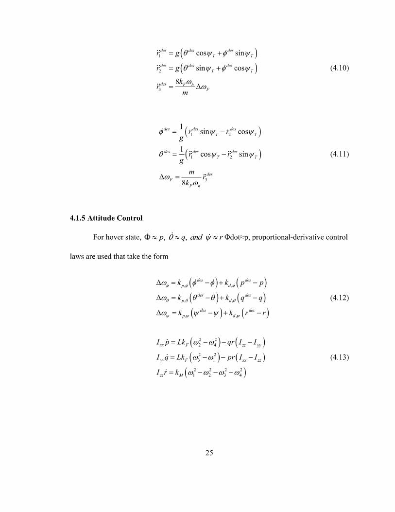
4.1.5 Attitude Control

For hover state, , , p q and r Φdot≈p, proportional-derivative control

laws are used that take the form

, ,

, ,

, ,

des desp d

des desp d

des desp d

k k p p

k k q q

k k r r

(4.12)

2 22 4

2 23 1

2 2 2 21 2 3 4

xx F zz yy

yy F xx zz

zz M

I p Lk qr I I

I q Lk pr I I

I r k

(4.13)

26

From the equation above the result of the ω desire are obtainable.

1

2

3

4

1 0 1 11 1 0 11 0 1 11 1 0 1

desh F

des

des

des

(4.14)

4.2 Dynamics Model Simulation

In this section, numerical simulation results for validation of the dynamic and

control model discussed in the previous section are presented. The parameters used for

the simulation are shown below in the Table 4.2.1.

Kpx=1 Kpy=1 Kpz=1

Kdx=1 Kdy=1 Kdz=1

kF=6.11*10-8 N/(r/min2). KM=1.5*10-9 N*m/(r/min2) Km=20

m=1.08 kg g=9.8 m/s2 L=0.22m

Table 4.2.1 Parameters of the dynamics model

Based on the dynamic model of the quadrotor, the control model was developed

in the MATLAB Simulink. The AppendixⅡhows details of the Simulink model of

quadrotor. For the simulation, the quadrotor flies from initial location (0,0,0) to goal

location (10,10,10) and hovers at the point (10,10,10).The distance units mentioned here

27

are in meters. The Fig. 4.4 shows the actual path taken by the quadrotor as it moves from

the intial to the goal location.

Figure 4.4 Simulation result showing the trajectory of the UAV

Fig. 4.5, Fig 4.6 and Fig 4.7 repectively show the plots of x, y, z locations of the

quadrotor versus time as the quadrotor moves from the intial to the desired location.

02

46

810

0

5

100

2

4

6

8

10

12

x(m)y(m)

z(m

)

28

Figure 4.5 Simulation result showing the x location of the quadrotor versus time

0 10 20 30 40 50 60 70 80 90 1000

2

4

6

8

10

12

t(s)

x(m

)

29

Figure 4.6 Simulation result showing the y location of the quadrotor versus time

0 10 20 30 40 50 60 70 80 90 100-2

0

2

4

6

8

10

12

t(s)

y(m

)

30

Figure 4.7 Simulation result showing the z location of the quadrotor versus time

In order to further verify the dynamics and control model with respect to tracking

a desired trajectory (rather goal location as above), the quadrotor was commanded to

move in a circle with center at (5, 0) and radius 5 m. The Fig. 4.8 shows the simulation

result of the desired and actual trajectory of the quadrotor following a circular trajectory.

The Fig. 4.9 shows the simulation result show the desired x and actual x for this circular

tracking. The Fig 4.10 shows the simulation result show the desired y and actual y for this

circular tracking.

0 10 20 30 40 50 60 70 80 90 100-2

0

2

4

6

8

10

12

t(s)

y(m

)

31

Figure 4.8 Simulation result showing the desired (shown in red) and actual trajectory (shown in blue) of a quadrotor following the circular trajectory

-2 0 2 4 6 8 10 12-6

-4

-2

0

2

4

6

x(m)

y(m

)

32

Figure 4.9 Simulation result showing the desired x (shown in red) and actual x (shown in

blue) of the quadrotor following a circular trajectory

33

Figure 4.10 Simulation result showing the desired y (shown in red) and actual y (shown

in blue) of the quadrotor following a circular trajectory

The control model was further verified showing quadrotor move from rest to a set

of desired locations and land again. The Fig. 4.11 shows the simulation of quadrotor’s

motion. The quadtor took off at the point (0, 0, 0) flew up to the point (0, 0, 10) then

turned and moved to the point (10, 10, 10) and then landed at the point (10, 10, 0), The

unit used is meter.

34

Figure 4.11 Simulation result of the quadrotor’s motion following a set of desired

locations

The above numerical simulations demonstrated that the quadrotor was able to

navigate to any desired way-point locations and follow any desired trajectory.

0

5

10

15

0

5

10

150

2

4

6

8

10

12

x(m)y(m)

z(m

)

35

Chapter 5

Trajectory Design and Optimization

5.1 Trajectory design

As previously stated in the Chapter 4, the Dubins curve is composed of S straight

line segment, circular arc to the left, L, and circular arc on the right side, R as shown in

Fig. 5.1 shown:

Figure 5.1 The sketch of Dubins Curve

36

It may be noted that the unit for distance considered in this thesis is meters. For

this thesis, the desired area is identified as a square area L (length) * W (width) =50 m*50

m as shown in Fig. 5.2:

Figure 5.2 Sample coverage area

To plan path for such a coverage area, the each path segment is designed to be

composed of a straight line segment, a semi-circular arc, followed by a straight line

segment as shown in the Fig. 5.3:

37

Figure 5.3 The sketch of a segment of the path

The overall path is obtained as shown in Fig. 5.4. Initial location of the UAV is

(0, 5). The quadrotor is required to initiate from this point into the desired area. The

quadrotor flies up in a straight line to reach the point (0, 55). Total distance for the linear

segment is 50. Then the UAV turns right to follow a semi-circular arc with radius equal

to 5. It may be noted that the sensor coverage/footprint area for the UAV is considered to

be 10 meters in diameter. After the quadrotor reachs the point (10, 55), it then flies in a

straight line. These motions are repeated to completely finish the coverage task.

38

Figure 5.4 Path planning of the UAV for the coverage problem

5.2 Optimization of Trajectory Parameters

Once the path or trajectory has been planned, the next step is to obtain trajectory

parameters such as velocity and acceleration so as to minimize the overall time required

to finish the mission. It may be noted that the trajectory parameters need to be optimized

while keeping in view the constraints of the quadrotor dynamics. The overall trajectory is

comprised of three kinds of movements as shown in Fig.5.5:

39

Figure 5.5 Classification of motions in the UAV trajectory

5.2.1 Segment 1: Curve Segment

For the curve segment, a semi-circular trajectory is designed. As previously

discussed in Chapter 4, a simulation was designed to track the circular trajectory. The

circular trajectory would be followed at a constant speed. The challenge is to determine

the maximum velocity that can be allowed in presence of the dynamic of quadrotor. This

maximum velocity can be obtained through the experiment with the Simulation model.

The designed curve is a semi-circular with radius equal to 5 m. The quadrotor will

track this circle with a constant linear speed Vcircle. The maximum speed that can track

40

this circle can be found via performing simulations with increasing magnitudes of

velocities. The results from these simulation experiments are shown in Fig.5.6 to Fig.5.10

which shows the trajectory followed by the UAV. The velocities were set to 0.1 m/s, 0.2

m/s, 0.3 m/s, 0.4 m/s and 0.5 m/s.

Figure 5.6 Trajectory followed by the UAV for magnitude of velocity equal to 0.1 m/s

41



42



43

The maximum errors between these real path and trajectory are 0.0005, 0.0139,

0.0539, 0.1318 and 0.32. We can see, as expected, that the error increases the speed

increases. Because the maximum acceptable error is 0.2, so 0.4 m/s is the maximum

linear velocity chosen for the quadrotor to follow the semi-circular trajectory.

The radius is 5 m. The constant magnitude of velocity to move on this trajectory

is 0.4 m/s. For the half circle, the minimum time needed is:

* 3.14*5 39.250.4circle

circle

rt sV

(5.4)

5.2.2 Segment 2: Straight line

Figure 5.11 Segment 2: Straight line

44

These two straight line movements shown in the above Fig. 5.11 consists of two

segments: acceleration motion and deceleration motion. For motion labeled 1 in the

figure, the quadrotor flies into the desired area from the initial point (0, 5). First, the

quadrotor flies with the acceleration a1 for t1 time. At time t1 the velocity is equal to v1.

Then, the quadrotor switches to fly with the deceleration a2 for t2 time and reaches the

point (0, 55). At time t2, the velocity is v2. This is the same velocity with which the

quadrotor flies during the curved segment of motion. The quadrotor then accelerates and

decelerates (as discussed in next Section: Segment 3). The final segment, shown as

Number 2 in the above figure, is exactly inverse of the first segment. Finally, the

quadrotor stops at the point (50, 5).

Now, the question arises what should these acceleration and deceleration be so as

to minimize the time take to travel this segment of path while ensuring that the UAV

satisfies all its dynamics constraints. For this thesis, the method based on Langrage

multiplier is used to obtain the maximum or minimum value of a mathematical function

in presence of constraints. With the set of Langrage multiplier, a new equation set or

objective function is obtained. For No. 1 straight line, the objective is to minimize the

time, i.e.,:

1 2 1 2( , )f t t t t (5.5)

The dynamics of the motion is obtained using kinematic equations for motion of

particles, as follows:

45

1 1 1

21 1 1

2 1 1 2 2

22 1 1 2 2 2

1 2

12

12

v a t

s a t

v a t a t

s a t t a t

s s L

(5.6)

So:

2 21 1 1 1 2 2 2

2 1 1 2 2

1 12 2

a t a t t a t L

v a t a t

(5.7)

And, also, the maximum acceleration constraint due to dynamics of the aircraft

poses the following constraints:

1 max

2 max

a aa a

(5.8)

To get the limited function:

2 21 1 2 1 2 1 1 1 1 2 2 2

2 1 2 1 2 1 1 2 2 2

3 1 2 1 2 1 max

4 1 2 1 2 2 max

1 1( , , , )2 2

( , , , )( , , , )( , , , )

g t t a a a t a t t a t L

g t t a a a t a t vg t t a a a ag t t a a a a

(5.9)

46

So, the augmented cost function is:

1 2 1 2 1 2 1 2 1 1 1 2 1 2 2 2 1 2 1 2 3 3 1 2 1 2 4 4 1 2 1 2( , , , ) ( , , , ) ( , , , ) ( , , , ) ( , , , ) ( , , , )(5.10)F t t a a f t t a a g t t a a g t t a a g t t a a g t t a a

The optimization is carried by simultaneously solving:

1

2

1

2

1

2

3

4

/ 0/ 0/ 0/ 0/ 0/ 0/ 0/ 0

F tF tF aF aFFFF

(5.11)

In order to obtain the maximum value of the acceleration the quadrotor can

provide, tests were done using the simulation model. The results are shown in the

following figures. The values of the acceleration were set as 1.5 m/s2, 2.0 m/s2 and 2.5

m/s2. The maximum rotor speed is set to 130 rad/s. As the Fig. 5.12-5.14 shown, the rotor

speed will increase as the acceleration increase. The rotor speed required is bigger than

130 rad/s when the acceleration equal to 2.5 m/s2. So the maximum acceleration the

quadrotor can provide is 2.0 m/s2.

47

Figure 5.12 The rotors’ speed simulation at the acceleration equal to 1.5 m/s2

48



49

So, the maximum acceleration constraint is chosen as:

2max 2 /a m s (5.12)

Also set:

250 , 0.4 /L m v m s (5.13)

The 2v is set to 0.4m/s from the circular segment of the motion. Substituting the

above values, a set of function is obtained:

1 1 1 1 2 2 1

1 1 1 2 2 2 22

1 1 1 2 2 1 3

21 2 2 2 4

2 21 1 1 1 2 2 2

1 1 2 2 2

1 max

2 max

1 ( ) 01 ( ) 0

(0.5 ) 0

( 0.5 ) 0

0.5 0.5 00

00

a t a t aa t a t at t t t

t ta t a t t a t L

a t a t va aa a

(5.14)

So:

1

2

5.04.8

tt

(5.15)

The minimum time to cover the segment No. 1 straight line is t1+t2=5.0+4.8=9.8 s.

Because the motion of segment No.2 is the inverse motion of No.1, so the shortest time to

cover the same is 9.8 s.

50

5.2.3 Segment 3: straight line

The segment 3 is similar as to segment 2, the motion of quadrotor also comprises

of an acceleration motion followed by a deceeration motion. However, in segment 3, the

initial and final velocities both are 0.4 m/s.

The objective function is:

3 4 3 4( , )f t t t t (5.16)

The motion function is obtained using kinematic equations for motion of particles,

as follows:

3

4 3 3 3

23 3 3 3 3

5 4 4 4

24 4 4 4 4

3 4

0.4

12

12

vv v a t

s v t a t

v v a t

s v t a t

s s L

(5.17)

So:

3 3 4 4

2 23 3 3 3 3 4 4 4

01 10.4 (0.4 )2 2

a t a t

t a t a t t a t L

(5.18)

51

And also:

1 max

2 max

a aa a

(5.19)

The limited function:

2 21 3 4 3 4 3 3 3 3 3 4 4 4

2 3 4 3 4 3 3 4 4

3 3 4 3 4 3 max

4 3 4 3 4 4 max

1 1( , , , ) 0.4 (0.4 )2 2

( , , , )( , , , )( , , , )

g t t a a t a t a t t a t L

g t t a a a t a tg t t a a a ag t t a a a a

(5.20)

So, the augmented cost function is:

3 4 3 4 3 4 3 4 1 1 3 4 3 4 2 2 3 4 3 4 3 3 3 4 3 4 4 4 3 4 3 4, , , ( , , , ) ( , , , ) ( , , , ) ( , , , ) ( , , , ) 5.21F t t a a f t t a a g t t a a g t t a a g t t a a g t t a a

The optimization is carried by simultaneously solving:

3

4

3

4

1

2

3

4

/ 0/ 0/ 0/ 0/ 0/ 0/ 0/ 0

F tF tF aF aFFFF

(5.22)

52

From the simulation model:

2max 2 /a m s (5.23)

Also set:

3 550 , 0.4 / , 0.4 /L m v m s v m s (5.24)

Substituting the above values, a set of function is obtained:

1 3 3 3 4 2 3

1 3 3 4 4 2 4

21 3 3 4 2 3 3

21 4 2 4 4

2 23 3 3 3 3 4 4 4

3 3 4 4

3

4

1 (0.4 ) 01 (0.4 ) 0

1( ) 021( ) 02

1 10.4 (0.4 ) 50 02 2

02 02 0

a t a t aa t a t a

t t t t

t t

t a t a t t a t

a t a taa

(5.25)

So:

3

4

4.84.8

t st s

(5.26)

The minimum time to scan one of the straight lines in segment 3 is

t3+t4=4.8+4.8=9.6 s.

53

The desired area is set as L*W=50*50 square area. The trajectory for coverage

scanning is as shown before in the Fig.5.4. The trajectory of this quadrotor is known. It

made 5 half circle curves. It needed time tcurve:

39.25*5 196.25curvet s (5.27)

The quadrotor that flied into the area from (0, 5) to (0, 55) and moved out from

(50, 55) to (50, 5), it needed time tsegment2:

2 9.8*2 19.6segmentt s (5.28)

Besides those above, the quadrotor also moves 4 times in a straight line same as

the segment 3 as previously discussed. For this segment movement it need time tsegment3:

2 9.6*4 38.4segmentt s (5.29)

So the total time for the quadrotor covering L*W=50*50 square area is:

t=236.61 s (5.30)

5.3 Simulation Results

5.3.1 Segment 1: Curve Segment

Fig. 5.15 shows the simulation result of the desired magnitude of velocity and

actual magnitude of velocity in the circular segment of the trajectory. The purple line

shows the desired magnitude of velocity which is 0.4 m/s. The yellow line shows the

actual magnitude of velocity. The errors are less than 0.05 m/s. Fig. 5.16 shows the

simulation result of the desired path and the actual path in circular segment of the

54

trajectory. Red line is the desired trajectory and the blue line shows the actual path. The

actual time to track this segment is 38.89 s.

Figure 5.15 Simulation result of the desired velocity and the actual velocity in the

circular segment

55

Figure 5.16 Simulation result of the desired path and the actual path in the circular

segment


Fig. 5.17 shows the simulation result of the desired magnitude of velocity (or

speed) and the actual speed in tracking Segment 2 that represents a straight line. The red

line shows the desired speed. The blue line shows the actual speed. The errors are less

than 0.5 m/s. Fig.5.18 shows the simulation result of the desired acceleration and the

actual acceleration in tracking Segment 2 of the trajectory. The red line shows the desired

acceleration. The blue line shows the actual acceleration. Fig. 5.19 shows the simulation

56

result of the desired path and actual path in tracking Segment2: straight line. Red line is

the desired trajectory and the blue line shows the actual path. The errors are less than

0.1m. The actual time to track this segment is 98 s.

Figure 5.17 Simulation result of the desired velocity and the actual velocity in

Segment 2 (straight line motion)

57

Figure 5.18 Simulation result of the desired acceleration and the actual

acceleration in Segment 2 (straight line motion)

58

Figure 5.19 Simulation result of the desired trajectory and the actual path in

Segment 2 ( straight line motion)


Fig. 5.20 shows the simulation result of the speed and the actual speed in tracking

the Segment 3 of the motion which is again a straight line. The red line shows the desired

speed. The blue line shows the actual speed. The errors are less than 0.5 m/s. Fig.5.21

shows the simulation result of the desired acceleration and the actual acceleration. The

red line shows the desired acceleration. The blue line shows the actual acceleration. Fig.

5.22 shows the simulation result of the desired path and actual path in tracking the

59

desired trajectory in Segment3 of the motion. Red line is the desired trajectory and the

blue line show the actual path. The errors are less than 0.09 m. The actual time to track

this segment is 96 s.

Figure 5.20 Simulation result of the desired velocity and the actual velocity in

Segment 3 ( straight line motion)

60

Figure 5.21 Simulation result of the desired acceleration and the actual

acceleration in Segment 3 (straight line motion)

61

Figure 5.22 Simulation result of the desired trajectory and the actual path in

Segment 3 (straight line motion)

5.3.4 Overall simulation

Fig. 5.23 shows the trajectory and the actual path for coverage the complete area.

The blue line shows the desired trajectory and the red line show the real path. As shown

in the figure, the real path closely tracked the trajectory.

62

Fig. 5.23 The desired and actual trajectory for coverage of the complete area

The following Figs. 5.24 show the area covered as the UAV tracks each of the

segments. The total time used for covering this area is 234.81 s.

63

Figure 5.24 Simulation result showing the area covered as the UAV tracks each of

the segments

64

Chapter 6

Conclusions and Future work

6.1 Conclusions

The thesis focused on solving two problems: i) obtaining a dynamic model of the

quadrotor, and ii) the planning of the path, and the optimiastion of the path planning.

In the first problem, the dynamics of the quadrotor was analyzed and then a

controller based on PID method was developed. In this section, the parameters were

chosen to make this simulation model to be nearly identical to the real quadrotor. Then,

point-to-point navigation as well as trajectory tracking experiments were performed using

the simulation model developed based on the dynamics of the quadrotor. The results

showed that this model worked well.

For second problem, the trajectory for exhaustive coverage of a specified area was

designed. The parameters of the trajectory were identified, and the Langrage multiplier

algorithm was utilized to obtain those parameters that minimized the total time taken to

traverse the entire trajectory. The trajectory was divided into three main parts, which

were calculated individually. During this calculation, the experiment on the simulation

model was used to determine the maximum velocity within the dynamic constraints of

65

the quadrotor (that limits the acceleration) to follow a half circle with radius equal to 5

meters. This velocity was found to be 0.4 m/s. The maximum acceleration of the

quadrotor, based on the dynamical constraints, was assumed to be 2.0 m/s2. Based on

those data, the minimum time for the quadrotor to finish each part was calculated based

on a Lagranian formulation. From this, an example scenario that required the quadrotor to

cover an area of L*H=50 m*50 m was designed. The minimum time to finish this area

was found, which t=236.61 s. From the simulation we know the simulation model to scan

this area need time 234.81 s. There were some errors between model and real quadrotor

because of the choice of parameters. This solution can be used in the future for other

develop techniques for other kinds coverage control problems.

6.2 Contributions

The contributions of this thesis are twofold: i) the thesis developed a MATLB

Simulink based simulation platform for control and navigation of a quadrotor UAV. The

model makes use of realistic dynamic model of the UAV and a controller based on PID

method that helps the UAV track a desired trajectory. ii) the thesis proposed a trajectory

to exhaustively cover a rectangular search area, and then developed a mechanism to

optimize the parameters of the trajectory so that the entire trajectory is traversed in

minimum time.

66

6.3 Future Works

There is a lot of interest recently on use of quadrotors for carrying out a number of

tasks such as package delivery, search and rescue, and monitoring. A lot of research still

needs to be carried out before the UAVs can be used in operational environment that

involve path planning and collision avoidance.

There has been a lot of research recently on designing the control system for a single

UAV and extending that to multiple UAVs. This thesis used a single quadrotor to finish

the coverage task. In the future, multiple quadrotors working together to accomplish the

task can be considered which will result in more time-efficient operation.

A lot of work has been carried out recently on development of sensors recently. These

sensors are have better performance, more efficient, cheaper, and lighter. The sensor can

now to be used to measure the light (vision) and the temperature (infra-red). These

advanced sensors can be placed on the quadrotor, so that the area can be patrolled for

monitoring hot-spots. Similarly, infra-red sensors can be used to find a lost person in vast

area where manual ground search is difficult. .

67

References

[1] A. Lyle, "Air Force officials announce remotely piloted aircraft pilot training

pipeline," Secretary of the Air Force Public Affairs, 2010

[2] D. Pines and F. Bohorquez, “Challenges facing future micro air vehicle development”,

AIAA J. Aircraft, vol. 43, no. 2, pp. 290–305, 2006.

[3] E. A. Poe, “The Raven”, 1845

[4] T. Lee, M. Leok and N. Harris McClamroch, “Geometric Tracking Control of a

Quadrotor UAV on SE(3)”, 49th IEEE Conference on Decision and Control, pp. 5420-

5425, 2010

[5] D. Quick, “Coaxial Rotor System: the future of helicopter design”, 2008

[6] A. Janetzko, “Wingcopter Fixed-Wing-Airplane/Quadcopter Fusion VTOL UAV,”

Aircraft platforms, December 7, 2012.

[7] G. Hoffmann, H. Huang, S. Waslander, and C. Tomlin, “Quadrotor Helicopter Flight

Dynamics and Control: Theory and Experiment”, AIAA Guidance, Navigation and

Control Conference and Exhibit, pp. 1, 20, Aug. 2007.

68

[8] M. A. Batalin and G. S. Sukhatme, “Coverage, Exploration and Deployment by a

Mobile Robot and Communication Network,” Proceedings of the International Workshop

on Information Processing in Sensor Networks, pp. 376-391, Apr. 2003

[9] D. Pines and F. Bohorquez, “Challenges facing future micro air vehicle development,”

AIAA Journal of Aircraft, vol. 43, no. 2, pp. 290–305, 2006

[10] E. Altug, J. Ostrowski, and C. Taylor, “Quadrotor Control Using Dual Camera

Visual Feedback," in 2003 IEEE International Conference on Robotics and Automation,

vol. 3, pp. 4294-4299, 2003.

[11] P. E. I. Pounds, “Design, Construction and Control of a Large Quadrotor Micro Air

Vehicle,” A thesis submitted for the degree of Doctor of Philosophy of the Australian

National University, pp. 36, Sep. 2007

[12] E. Altug, J. P. Ostrowski, R. Mahony, “Control of a Quadrotor Helicopter Using

Visual Feedback,” IEEE International Conference on Robotics & Automation, pp.72-76,

May 2002.

[13] B. Y. N. Michael, D. Mellinger, Q. Lindsey, and V. Kumar, “The GRASP Multiple

Micro-UAV Test Bed," IEEE Robtics & Automation Magazine, vol. 17, no. 3, pp. 56-65,

2010.

[14] K. Karwoski, “Quadrocopter Control Design and Flight Operation,” Massachusetts

Institute of Technology, pp.1-2, Aug.2011

[15] G. Hoffmann, H. Huang, S. Waslander, and C. Tomlin, “Quadrotor Helicopter Flight

Dynamics and Control: Theory and Experiment," AIAA Guidance, Navigation and

Control Conference and Exhibit, pp. 1-20, Aug. 2007.

69

[16] S. L. Waslander, J. S. Jang, C. J. Tomlin, “Multi-Agent X4-Flyer Testbed Control

Design: Integral Sliding Mode vs. Reinforcement Learning,” IEEE Conference on

Intelligent Robots and Systems, 2009

[17] N. Guenard, T. Hamel, V. Moreau, and S. A. France, “Dynamic Modeling and

Intuitive Control Strategy for an X4-fyer," in ICCA'05 International Conference on

Control and Automation, pp. 1-6, 2005.

[18] E. Nice, “Design of a Four Rotor Hovering Vehicle," Ph.D. dissertation, Cornell

University, 2004.

[19] A. Blum, P. Raghavan, and B. Schieber, “Navigating in unfamiliar terrain,” In STOC,

pp. 494-504, 1991.

[20] JY. Potvin, “A review of bio-inspired algorithms for vehicle routing,”Bio-inspired

Algo. Vehic. Routing Problem, vol. 161, pp. 1–34, 2009.

[21] J. Tisdale, Z. Kim, and J. Hedrick, “Autonomous UAV path planning and

estimation,” IEEE Robotics Automation Magazine, vol. 16, no. 2, pp. 35 –42, 2009.

[22] S. Poduri and G. S. Sukhatme, “Constrained coverage for mobile sensor networks,”

in Proc. IEEE Intl. Conf. Robot. Autom., 2004, pp. 165–172.

[23] E. Yanmaz, “Robert Kuschnig On Path Planning Strategies for Networked

Unmanned Aerial Vehicles,” Ieee infocom, pp212-216, 2011.

[24] L. E. Dubins. “On curves of minimal length with a constraint on average curvature,

and with prescribed initial and terminal positions and tangents,” American Journal of

Mathematics, pp. 497–516, 1957.

[25] J. A. Reeds and L. A. Shepp. “Optimal paths for a car that goes both forwards and

backwards.” Pacific J. Math., pp. 367–393, 1990.

70

[26] J.D. Boissonnat, A. C´er´ezo, and J. Leblond. “Shortest paths of bounded curvature

in the plane”, J. Intelligent and Robotic Systems, pp. 5–20, 1994.

[27] H. Sussmann and G. Tang. “Shortest paths for the Reeds- Shepp car: A worked out

example of the use of geometric techniques in nonlinear optimal control,” Technical

Report SYNCON 91-10, Dept. of Mathematics, Rutgers University, 1991.

[28] D. J. Balkcom and M. T. Mason. “Time optimal trajectories for bounded velocity

differential drive vehicles”, Int. J. Robot. Res., pp.199–218, March 2002.

[29] H. Chitsaz, S.M. LaValle, D.J. Balkcom, and M.T. Mason. “An explicit

characterization of minimum wheel-rotation paths for differentialdrives”, In Proceedings

12th IEEE International Conference on Methods and Models in Automation and Robotics,

2006.

[30] N. Michael, D. Melinger, Q. Lindsey and V. Kumar, “The GRASP Multiple Micro

UAV Testbed”, Robotics & Automation Magazine, IEEE, pp.56-65, 2010.

[31] A. Nemati and M. Kumar, “Modeling and control of a single axis tilting quadcopter”,

In American Control Conference (ACC), pp. 3077-3082, 2014, June.

[32] A. Nemati and M. Kumar, “Non-Linear Control of Tilting Quadcopter Using

Feedback Linearization Based Motion Control”, Dynamic System and Control

Conference (DSCC), 2014.

71

Appendix A

Parameters of the dynamics model

kp_x=1;kp_y=1;kp_z=1

kd_x=1;kd_y=1;kd_z=0.3

kf=6.11*10^(-4)*3600

km=1.5*10^(-9)*3600

m=1.08

wH=sqrt(m*9.8/(kf*4))

g=9.8

kp_pitch=0.01;kd_pitch=1;kp_roll=0.01;kd_roll=1;kp_yaw=1;kd_yaw=0.01

dt=0.1

L=0.22

i_xx=m*2*(L^2);i_yy=m*2*(L^2);i_zz=m*4*(L^2)

kM=20

72

Appendix B

The system for the dynamics simulation

The UAV dynamics simulation model

73

Subsystem of the dynamics simulation

PD-Position Subsystem

74

Position Control Subsystem

Subsystem 5

75

Subsystem 6

Subsystem 2

76

Subsystem 3

Subsystem4

77

Subsystem 7

A Thesis entitled Optimal Path Planning and Control of ...

Documents

Transcript of A Thesis entitled Optimal Path Planning and Control of ...