International Journal of Fatigue 47 (2013) 300–307

Contents lists available at SciVerse ScienceDirect

International Journal of Fatigue

journal homepage: www.elsevier .com/locate / i j fa t igue

A probabilistic model for the onset of High Cycle Fatigue (HCF) crackpropagation: Application to hydroelectric turbine runner

Martin Gagnon a,⇑, Antoine Tahan a, Philippe Bocher a, Denis Thibault b

a École de Technologie Supérieure (ÉTS), Montréal, Québec, Canada H3C 1K3b Institut de Recherche d’Hydro-Québec (IREQ), Varennes, Québec, Canada J3X 1S1

a r t i c l e i n f o a b s t r a c t

Article history:Received 23 March 2012Received in revised form 17 September2012Accepted 18 September 2012Available online 3 October 2012

Keywords:High Cycle Fatigue (HCF)ReliabilityFORM/SORMLEFM

0142-1123/$ - see front matter � 2012 Elsevier Ltd. Ahttp://dx.doi.org/10.1016/j.ijfatigue.2012.09.011

⇑ Corresponding author.E-mail address: martin.gagnon.8@ens.etsmtl.ca (M

A fatigue reliability model for hydroelectric turbine runners is presented in this paper. In the proposedmodel, reliability is defined as the probability of not exceeding a threshold above which HCF contributeto crack propagation. In the context of combined LCF–HCF loading, the Kitagawa diagram is used as thelimit state threshold. Two types of crack geometries are investigated: circular surface flaw and embeddedflaw in a semi-infinite medium. The accuracy of FORM/SORM approximations was considered acceptablefor engineering purpose in our application given the minimal numerical burden posed by such a methodcompared to Monte Carlo simulations. Our results show that the probability of an embedded flaw close tothe surface has a major influence on reliability. Furthermore, we observe that the assumption that crackgeometrical characteristics are independent leads to non-conservative results.

� 2012 Elsevier Ltd. All rights reserved.

1. Introduction

The reliability assessment of structural components is oftenlimited by our capacity to select relevant models and proper limitstates. In structures, such as large Francis hydroelectric turbinerunners, where the cost of downtime is high and in situ inspectionmethods are limited, cracks often reach a detectable size only afterthe onset of High Cycle Fatigue (HCF). Furthermore, because largeFrancis runners can sustain significant amount of damage withoutincurring safety issues, the main concerns are repair cost anddowntime. Hence, a crack must be repaired as soon as possible inorder to minimize the cost of repair and concurrently the time be-tween inspections must be maximized to reduce downtime. Thisleads to the following dilemma: if the HCF onset has occurred,longer time between inspection leads to longer cracks to repair;yet, if the component is inspected before the HCF onset, we incurdowntime and maintenance costs with limited information onthe state of the structure because the detectable flaw size is notreached. Therefore, we propose to move away from the typical fa-tigue limit, as commonly seen in SN curve and critical crack length,which do not adequately reflect this reality, in favor of a limit statedirectly related to the HCF onset.

In this paper, the HCF is defined as the contribution to crackpropagation by small amplitude stress cycles, leading to the rapidgrowth. In this case, the Low Cycle Fatigue (LCF) part of the loading

ll rights reserved.

. Gagnon).

is composed of the large amplitude stress cycles which contributeinitially to the crack growth. These large amplitude cycles are lessfrequent than the small amplitude cycles of the HCF part of theloading. A schematic representation of an LCF + HCF combinationis presented in Fig. 1[1]. We observe, in Fig. 2, that this representa-tion is similar to the strain measured during a typical loading se-quence if the startup phase of the sequence is neglected. Theoverall amplitude of the transient observed during the startupphase is directly related to the control scheme used [2,3] and itsimpact on the runner reliability will not be investigated in this pa-per. For a typical hydroelectric turbine runner, we assume that theHCF will induce a rapid crack growth to a size above detection lim-its, which will then becomes proportional to HCF loading ratherthan to a limited number of transients LCF events. Notice that thisdefinition is compatible with the one used in the review work doneby Nicholas [4].

Reliability, for its part, is generally defined as: ‘‘The ability of asystem or component to perform its required functions under sta-ted conditions for a specified period of time’’ [5]. For a large Francisturbine runner, because cracks need to be repaired as soon as de-tected to minimize cost, the limit state for reliability becomesthe onset of HCF crack propagation after which a flaw will rapidlybecome a detectable crack. The problem is illustrated in Fig. 3using British Standard BS7910:2005 [6] deterministic crack growthprocedure and the loading presented in Fig. 2 [2]. The LCF onlycurve represents the results for the loading with minimal time atthe maximum opening condition and the HCF + LCF curve, on theother hand, includes 24 h of operation time at this condition for

Fig. 1. Schematic example of combined LCF + HCF loading.

Fig. 2. Example of loading measured on a large Francis runner.

Fig. 3. Deterministic crack growth example using Fig. 2 loading.

Fig. 4. Schematic Kitagawa diagram.

M. Gagnon et al. / International Journal of Fatigue 47 (2013) 300–307 301

each loading block. In this case, we observe that using any criticalcrack size above the HCF onset point could be almost equallyacceptable but would hide the real limit state and would cloudour understanding of the reliability problem. Obviously, we havenot accounted for stress gradient and other factors which would

affect crack growth but this simple example illustrates the diffi-culty of assigning a arbitrary critical crack length when, in facts,the moment of interest is the HCF onset.

Kitagawa and Takahashi [7] established that the thresholdwhich differentiates a propagating from a non-propagating crackis characterized by at least two thresholds; the first threshold isthe stress intensity range for crack growth DKth as defined by Lin-ear Elastic Fracture Mechanics (LEFM), and the second threshold isthe fatigue limit, which usually corresponds to 107 stress cycles formaterials exhibiting an endurance limit. The limit state defined byKitagawa and Takahashi [7] can also be extended to include otherparameters like notch effect [8] and multi-axial criteria [9]. We re-fer the reader to the work of Atzori and Lazzarin [10] for an over-view of the experimental data available in the literature thatsupport such limit. In the present study, the limit state for HCF isderived only from the thresholds established by Kitagawa andTakahashi [7], combined with the correction factor developed byEl Haddad et al. [11], which accounts for short crack propagation.This limit state can be visualized on a two-dimensional diagramwith defect size and stress range for axes, as shown in Fig. 4.

In order to use this model in a probabilistic approach, we pro-pose the use of an isoprobabilist transformation combined withthe Hasofer–Lind index to obtain the probability of exceeding aspecified threshold using First- or Second-Order Reliability Meth-ods (FORM/SORM). The premise in this study is that defect geom-etry and size uncertainty have already been defined either frominspections data or probabilistic crack growth simulations. Thestudy of both inspection data and crack growth models are beyondthe scope of this paper. From that premise, the reliability assess-ment is reduced to the probability of exceeding a threshold whichfollow this general procedure:

1. Definition of the variables of interest, limit state and inputvariables.

2. Quantification of the uncertainty sources.3. Isoprobabilist transform.4. Most Probable Point (MPP) search.5. Reliability approximation.6. Sensitivity analysis and ranking of uncertainty sources.

Then, two application examples are investigated to assess thespeed and accuracy of the FORM/SORM approximations vs. theconventional Monte Carlo simulations. Finally, we conclude witha limited sensitivity analysis on some parameters consideredimportant for our application and the applicability of the devel-oped probabilistic criteria for the reliability assessment of largerotating machinery such as large Francis runner.

Fig. 5. Schematic probabilistic Kitagawa diagram.

302 M. Gagnon et al. / International Journal of Fatigue 47 (2013) 300–307

2. High Cycle Fatigue (HCF) reliability

To assess the fatigue reliability of a structure, the following ele-ments are needed: a properly defined limit state model, a reliabil-ity criterion and characterized uncertainty sources. In this study,the limit state is defined as the thresholds proposed by Kitagawaand Takahashi [7] combined with the correction factor developedby El Haddad et al. [11]. This correction factor accounts for shortcrack growth by asymptotically matching the LEFM thresholdand the fatigue limit. This limit state, commonly called the Kitaga-wa diagram, is shown in Fig. 4, and in it, the limit formed by theLEFM threshold is obtained from the stress intensity factor solutiondefined as follows:

DK ¼ Drffiffiffiffiffiffipap

YðaÞ ð1Þ

where DK is the stress intensity factor variation, Dr is the stress cy-cle range, a is the crack length and Y(a) is the stress intensity correc-tion factor for a given geometry. The limit state equation is obtainedby replacing DK by the LEFM threshold DKth in Eq. (1) which isrewritten as follows:

Drth ¼ DKthffiffiffiffiffiffipap

YðaÞð2Þ

We note that the values DKth is known to be influenced by thestress ratio R [12]. If needed, DKth could be modeled as a functionof R to account for change in the steady state conditions. However,the study of such variation is beyond the scope of this paper sincean hydroelectric turbine runner generally operates under ratherconstant and high R ratio most the time leading to concern onlyfor the worst steady state condition in the time interval of interest.In order to capture short crack growth, El Haddad et al. [11] pro-posed to asymptotically match the limits defined by LEFM and thefatigue limit Dr0 using the reference crack length a0 as a correctionfactor. The correction factor a0 is added to the crack length a in Eq.(2) to obtain:

Drth ¼ DKthffiffiffiffiffiffiffiffiffiffiffiffiffiffiffiffiffiffiffiffipðaþ a0Þ

pYðaþ a0Þ

ð3Þ

where the constant a0 represents the transition crack size betweenboth limits, and is obtained by solving the following equation:

a0 ¼1p

DKthDr0 Yða0Þ

� �2

ð4Þ

For infinite life, Dr0 is the endurance limit. However, in some cases,the limit state for a finite number of cycles N might also be of inter-est either because the number of cycles for infinite life might nothave been reached in a given time interval or because the materialhas no endurance limit. In those instances, a finite number of stresscycles N can be accounted for using the fatigue limit at N cyclesrather than the endurance limit. This approach is similar to themodel developed by Ciavarella and Monno [13]. In the current ap-proach, to account for a limited number of cycles N, Eqs. (3) and(4) can be rewritten as follows:

Drth ¼ DKthffiffiffiffiffiffiffiffiffiffiffiffiffiffiffiffiffiffiffiffiffiffiffiffiffiffiffiffiffip ðaþ a0ðNÞÞ

pYðaþ a0ðNÞÞ

ð5Þ

a0ðNÞ ¼1p

DKthDr0ðNÞ Yða0ðNÞÞ

� �2

ð6Þ

It is relevant to note that any of the parameters in Eqs. (5) and (6)can be used as an independent random variable. Now that the limitstate has been defined, the criteria for failure must be defined and isexpressed as follows:

gðxÞ 6 0 ð7Þ

with a probability of failure:

Pf ¼Z

gðxÞ60fXðxÞ dx ð8Þ

in which, x is an n-dimensional vector of random variables with ajoint density function fX(x). By defining the failure as the HCF onset,g(x) becomes:

gða;DrÞ ¼ Dr� DKonsetffiffiffiffiffiffiffiffiffiffiffiffiffiffiffiffiffiffiffiffiffiffiffiffiffiffiffiffiffip ðaþ a0ðNÞÞ

pYðaþ a0ðNÞÞ

ð9Þ

where DKth has been replaced by DKonset for generality to differen-tiate the onset from LEFM threshold DKth because in some case theonset could be different due to interaction between HCF and LCF cy-cles [1]. Furthermore, we observe that two time-dependant param-eters are found in Eq. (9). The first one is a0(N) which increases withtime because Dr0 decreases with the number of stress cycles N un-til it reaches the endurance limit. The second parameter is the de-fect size a which concurrently increases with time due to the LCFpart of the loading spectrum. To illustrate Eq. (9), the limit statewith the associated parameters uncertainties are shown in Fig. 5.

Then, to properly define the model, uncertainty sources must becharacterized. For the purpose of this study Dr0 and DKonset areconsidered deterministic which reduces the model in the simplestcase to two random parameters: defect size and stress range. Ourassumption is that for a given element of volume subjected to auniform stress level, the HCF onset will occur at the largest flawdue to the largest stress cycle in the HCF loading. For both randomvariables, the largest value uncertainty can be characterized usingthe Extreme Value Theory (EVT). Within EVT, two models can beused: the General Extreme Value (GEV) distribution and the Gen-eral Pareto Distribution (GPD). The GEV cumulative distributionis expressed as follows:

FðxÞ ¼ exp � 1þ nðx� lÞr

� ��1=n !

ð10Þ

where n 2 R is the shape factor, l 2 R is the location parameter andr > 0 the scale parameter. The case where n > 0 and n < 0 correspondrespectively to the Fréchet and Weibull distribution. Note that n = 0is a special case which leads to the Gumbel distribution for whichthe cumulative is reduced to:

FðxÞ ¼ exp �e�ðx�lÞ

r

� �ð11Þ

Because GEV distribution characterizes the uncertainty around asample largest event (i.e. block maxima), only a small part of theavailable data can be used for parameter estimation. This limitationcan be alleviated by the use of GPD model which characterizes the

Fig. 6. Schematic isoprobabilist space.

M. Gagnon et al. / International Journal of Fatigue 47 (2013) 300–307 303

observations exceeding a given threshold (i.e. peak-over-threshold).Using a GDP model, a larger part of the available data can be usedfor parameter estimation. The GPD cumulative probability distribu-tion is expressed as follows:

FðxÞ ¼ 1� 1þ nðx� lÞr

� ��1=n

ð12Þ

where n 2 R is the shape factor, l 2 R is the location parameter andr > 0 the scale parameter. The special case n = 0 corresponds to theexponential distribution which reduce Eq. (12) to the following:

FðxÞ ¼ 1� e�ðx�lÞ

r ð13Þ

We would like to note that the GEV distribution can be obtainedfrom the GPD or vice versa, using the assumption that the peaksover a high enough threshold follow a Poisson process [14]. Theexponential and Gumbel distribution are simplified versions of theirgeneralized counterpart. As such, the Gumbel distribution was cho-sen to model both random variables. Note that this distribution hasalready been used in the literature to model both the extremes ofload spectra [15] and the defect size [16,17]. This assumptionshould be reasonable for a wide range of applications because manydistributions, like the normal, log-normal and Weibull distribution,are approximately exponentially distributed above a high enoughthreshold [18,19]. However, there is no restriction on the distribu-tion to be used.

3. Isoprobabilist transformation and Hasofer–Lind reliabilityindex

Two numerical approaches can be used to solve the probabilityof HCF onset defined by Eq. (8) in the previous section. The ap-proaches can either be simulation-based, like the Monte Carlo(MC) simulation and its variants, or analytical, using approxima-tions like the First-Order Reliability Method (FORM) and the Sec-ond-Order Reliability Method (SORM). An advantage with thesimulation-based method, like the Crude MC, is that it asymptoti-cally converges to the exact values for a number of simulationsN ?1 but nevertheless has a drawback, common to all simula-tion-based methods, of possibly requiring a prohibitive numberof simulations in order to obtain reliable results, for a low-probability estimate. On the other hand, analytical methods arebased on the approximation of the probability of failure leadingto a minimal numerical burden in exchange for accuracy.

FORM/SORM approximations rely on the assumption that atransformation in the form U = T(X) exists, mapping the physicalspace to a standard space. The transformation is expressed asfollows:

Pf ¼Z

gðXÞ60f ðxÞ dx ¼

ZgðTðXÞÞ60

uðuÞ du ð14Þ

where u(u) is an n-dimensional standard normal density with inde-pendent components. Several such transformation methods areavailable. The Rosenblatt transform [20] was chosen in this studybecause of its flexibility to impose a dependency structures be-tween the random variables modeled using the copula theory. TheRosenblatt transform is defined as follow:

U ¼ TðXÞ ¼ T2ðXÞ � T1ðXÞ ð15Þ

T1 : Rn ! Rn

X # Y ¼

F1ðX1ÞF2ðX2jX1ÞF3ðX3jX1;X2Þ...

FnðXnjX1;X2; . . . ;Xn�1Þ

0BBBBBBB@

1CCCCCCCA

ð16Þ

T2 : Rn ! Rn

Y # U ¼

U�1ðY1ÞU�1ðY2Þ...

U�1ðYnÞ

0BBBBB@

1CCCCCA

ð17Þ

where X in Rn is a continuous random vector defined by its marginalcumulative distributions Fi and copula. It should be noted that theconditioning order in Eq. (16) will influence the shape limit statein the standard space U and impact the results of the FORM/SORMapproximation. Because the stress ranges are considered indepen-dent of the defect size, the assumption can be made that the ran-dom vector X has an independent copula. The independent copulaassumption simplifies the Rosenblatt transform and Eq. (15)becomes:

U ¼

U�1ðF1ðX1ÞÞU�1ðF2ðX2ÞÞ...

U�1ðFnðXnÞÞ

0BBBBB@

1CCCCCA ð18Þ

In the standard space U, the probability of failure can be obtainedeither with a linear approximation (FORM) or a quadratic approxi-mation (SORM) as shown in Fig. 6. In this space, the Most ProbablePoint (MPP) of failure, also named the design point u⁄, is located atthe shortest distance between the origin and the limit state g(U) = 0.The distance to the MPP is called the Hasofer–Lind reliability indexbHL.

The FORM approximation of the probability of failure Pf is calcu-lated directly from the Hasofer–Lind index bHL and is given by:

Pf ¼ 1�UðbHLÞ ¼ Uð�bHLÞ ð19Þ

where bHL = ku⁄k, U is the standard normal cumulative function andu⁄ = mink uk for g(U) 6 0. The main numerical burden of thisapproximation resides in finding the location of the design pointu⁄. Note that the results obtained with the FORM approximationare only accurate when the limit state is linear in the standard spaceU. Likewise, results from the SORM approximations are only accu-rate when the limit state at the design point is close to quadraticin the standard space U. Many formulation are available for SORMapproximations, three of which will be used in this paper: the Tveldformulation [21], the Breitung formulation [22], and the Hohenb-ichler formulation [23]. The SORM solution requires n(n + 1)/2 addi-tional function calls over the FORM approximation to compute themain curvatures around the design point in the standard space [24].

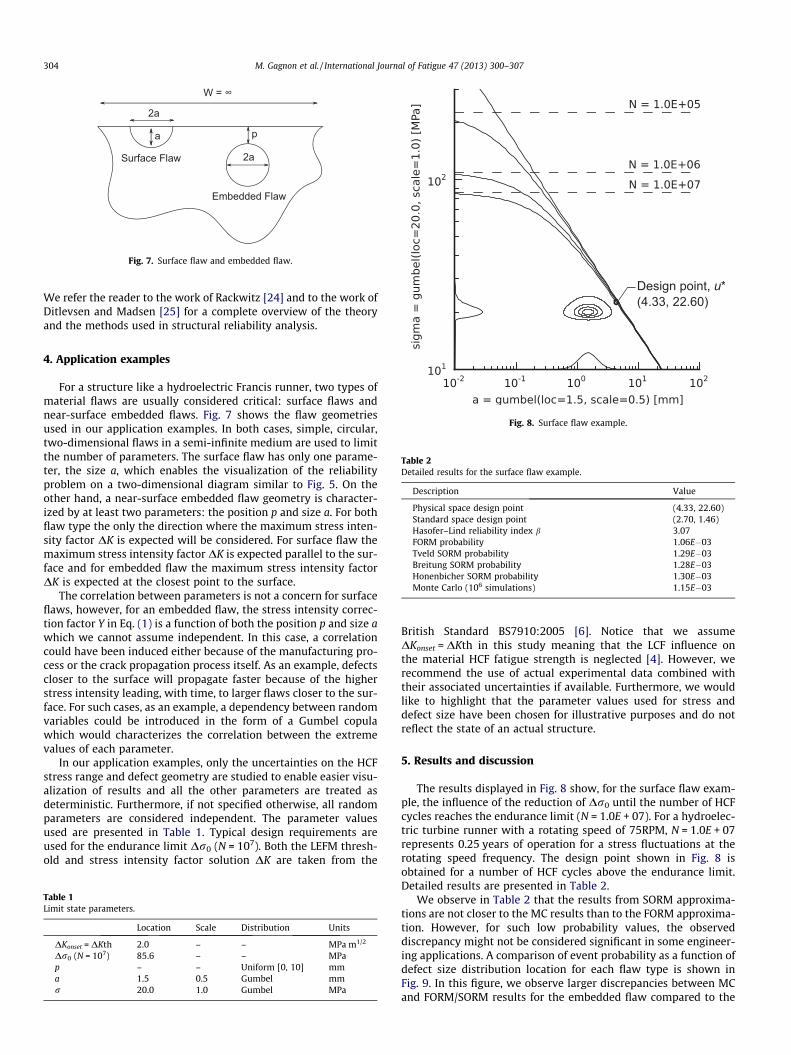
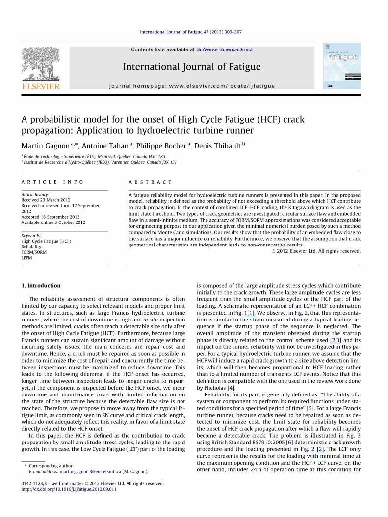
Fig. 7. Surface flaw and embedded flaw.

304 M. Gagnon et al. / International Journal of Fatigue 47 (2013) 300–307

We refer the reader to the work of Rackwitz [24] and to the work ofDitlevsen and Madsen [25] for a complete overview of the theoryand the methods used in structural reliability analysis.

Fig. 8. Surface flaw example.

Table 2Detailed results for the surface flaw example.

Description Value

Physical space design point (4.33, 22.60)Standard space design point (2.70, 1.46)Hasofer–Lind reliability index b 3.07FORM probability 1.06E�03Tveld SORM probability 1.29E�03Breitung SORM probability 1.28E�03Honenbicher SORM probability 1.30E�03Monte Carlo (106 simulations) 1.15E�03

4. Application examples

For a structure like a hydroelectric Francis runner, two types ofmaterial flaws are usually considered critical: surface flaws andnear-surface embedded flaws. Fig. 7 shows the flaw geometriesused in our application examples. In both cases, simple, circular,two-dimensional flaws in a semi-infinite medium are used to limitthe number of parameters. The surface flaw has only one parame-ter, the size a, which enables the visualization of the reliabilityproblem on a two-dimensional diagram similar to Fig. 5. On theother hand, a near-surface embedded flaw geometry is character-ized by at least two parameters: the position p and size a. For bothflaw type the only the direction where the maximum stress inten-sity factor DK is expected will be considered. For surface flaw themaximum stress intensity factor DK is expected parallel to the sur-face and for embedded flaw the maximum stress intensity factorDK is expected at the closest point to the surface.

The correlation between parameters is not a concern for surfaceflaws, however, for an embedded flaw, the stress intensity correc-tion factor Y in Eq. (1) is a function of both the position p and size awhich we cannot assume independent. In this case, a correlationcould have been induced either because of the manufacturing pro-cess or the crack propagation process itself. As an example, defectscloser to the surface will propagate faster because of the higherstress intensity leading, with time, to larger flaws closer to the sur-face. For such cases, as an example, a dependency between randomvariables could be introduced in the form of a Gumbel copulawhich would characterizes the correlation between the extremevalues of each parameter.

In our application examples, only the uncertainties on the HCFstress range and defect geometry are studied to enable easier visu-alization of results and all the other parameters are treated asdeterministic. Furthermore, if not specified otherwise, all randomparameters are considered independent. The parameter valuesused are presented in Table 1. Typical design requirements areused for the endurance limit Dr0 (N = 107). Both the LEFM thresh-old and stress intensity factor solution DK are taken from the

Table 1Limit state parameters.

Location Scale Distribution Units

DKonset = DKth 2.0 – – MPa m1/2

Dr0 (N = 107) 85.6 – – MPap – – Uniform [0, 10] mma 1.5 0.5 Gumbel mmr 20.0 1.0 Gumbel MPa

British Standard BS7910:2005 [6]. Notice that we assumeDKonset = DKth in this study meaning that the LCF influence onthe material HCF fatigue strength is neglected [4]. However, werecommend the use of actual experimental data combined withtheir associated uncertainties if available. Furthermore, we wouldlike to highlight that the parameter values used for stress anddefect size have been chosen for illustrative purposes and do notreflect the state of an actual structure.

5. Results and discussion

The results displayed in Fig. 8 show, for the surface flaw exam-ple, the influence of the reduction of Dr0 until the number of HCFcycles reaches the endurance limit (N = 1.0E + 07). For a hydroelec-tric turbine runner with a rotating speed of 75RPM, N = 1.0E + 07represents 0.25 years of operation for a stress fluctuations at therotating speed frequency. The design point shown in Fig. 8 isobtained for a number of HCF cycles above the endurance limit.Detailed results are presented in Table 2.

We observe in Table 2 that the results from SORM approxima-tions are not closer to the MC results than to the FORM approxima-tion. However, for such low probability values, the observeddiscrepancy might not be considered significant in some engineer-ing applications. A comparison of event probability as a function ofdefect size distribution location for each flaw type is shown inFig. 9. In this figure, we observe larger discrepancies between MCand FORM/SORM results for the embedded flaw compared to the

Fig. 9. Event probability vs. defect size for surface flaw and embedded flaw examples.

Fig. 10. Reliability index vs. defect size for surface flaw and embedded flawexamples.

ig. 11. Embedded flaw reliability index for deterministic distance from theurface.

M. Gagnon et al. / International Journal of Fatigue 47 (2013) 300–307 305

surface flaw. Nonetheless, these discrepancies might still be con-sidered negligible if we consider that the FORM results in Table 2are obtained using only 45 function calls, as compared to the 106

function calls needed to obtain a convergent MC estimate.Also, in Fig. 9, we might believe their is a lack of sensitivity in

the low probability region for both examples. However, the is onlydue to the non-linearity of the results which renders comparisonand visualization difficult across different level of probability.These difficulties can be alleviated by the use of the reliability in-dex b as a comparison basis instead of the event probability. Thereliability index can be visualized as a measure of the shortest dis-tance to the limit state in the standard space and is directly relatedto the probability of failure Pf. However, the Hasofer–Lind indexbHL, as defined previously, is only calculated during FORM/SORMapproximations. For an arbitrary probabilistic result, the index bcan be generalized using the following:

b ¼ U�1ð1� Pf Þ ¼ �U�1ðPf Þ ð20Þ

where Pf is the probability of an event obtained from an arbitrarymethod. The generalized reliability index offers a general criterionfor reliability comparison. We would like to refer the reader tothe work of Ditlevsen and Madsen [25] for more information onreliability index. The reliability index b as a function of defect sizedistribution location a for both flaw types using the values in Table 1and considering all random parameters independent is shown inFig. 10.

We observe lower reliability indexes for the surface flaw resultscompared to the embedded flaw results. These lower b valuesmight be misleading since a close to surface embedded flaw canbe more critical than a surface flaw. This is due to the random nat-ure of the position parameter p. The effect of both the defect size aand distance from the surface p can be observed in Fig. 11. Notethat the reliability index increases with the distance from the sur-face and decreases with the defect size. Compared to a surface flaw,an embedded flaw has a higher reliability index far from the sur-face and a lower one close to the surface. As a consequence, whenthe distance from the surface p is treated as a random variable, theprobability of a flaw occurring close to the surface can significantlyreduces the overall reliability index.

In such instances, the quantification of marginal distributionsmight be as important as the correlation structure between the de-fect size a and distance from the surface p. In our embedded flawexample, the defect size a and the distance from the surface p can-not be assumed independent without proper experimental valida-tion. Ignoring the relationship between random variables canproduce significant results bias. For example, the results from a

Fs

Fig. 12. Gumbel copula with a Kendall s = 0.60 (number of samples = 1000).

Fig. 13. Independent copula vs. Gumbel copula for the embedded flaw example.

306 M. Gagnon et al. / International Journal of Fatigue 47 (2013) 300–307

Gumbel copula with a Kendall s = 0.60 is shown in Fig. 12. The fig-ure represent one thousand random samples obtained from twouniform distributions. We observe that extreme values from bothdistribution tend to appear together with a level of dependencemeasured by the Kendall s coefficient. Similarly, in Fig. 13, a Gum-bel copula with a Kendall s = 0.60 is used to model the correlationbetween the flaw size and position such that large flaws will tendto appear close to the surface, resulting in a significantly lower reli-ability index compared to the results obtained for the embeddedflaw with an independent copula or the surface flaw. These resultshighlight the sensitivity of reliability results to such assumption,and even more so if the assumption cannot be validated with ob-served data.

6. Conclusions

A fatigue reliability model for HCF crack propagation in hydro-electric turbine runner was proposed in this paper. We establishedthat the HCF onset is the proper limit state for a hydroelectric tur-bine runner since the HCF onset marks the point in time after

which a flaw becomes a detectable crack. In the proposed model,the limit state is formed by the Kitagawa and Takahashi [7] dia-gram combined with the El Haddad et al. [11] correction factorwhich defines the region where, for a given set of parameters, acrack will not propagate. Applied in the context of a combinedLCF–HCF loading, the proposed model allows the evaluation ofthe fatigue reliability at any point in time, from the available infor-mation about material properties, defect size and HCF loading. Theaccuracy obtained using FORM/SORM approximations was com-pared to the results from crude MC simulations using two typicalflaw geometries. A lower accuracy was observed for the embeddedflaw geometry compared to the surface flaw geometry usingFORM/SORM approximations. However, in both cases, the resultsfollow the same overall trend as the crude MC simulations whichmight warrant their use over more numerically intensive simula-tion methods, given the minimal numerical burden inherent tosuch approximations.

The embedded flaw results have highlighted some of the diffi-culties associated with flaw geometries characterized by morethan one random parameter. First, we observed that even if a high-er reliability is expected for a flaw far from the surface, the pros-pect of a flaw close to the surface can lower significantlyreliability associated with embedded flaws making them morecritical than surface flaws. The results were first obtained by con-sidering the random variables independent which with furtherinvestigation proved to be a non-conservative assumption. In thestudy, a correlation between flaw size and position was inducedusing a Gumbel copula, such that large flaws tend to appear closeto the surface, and a significant reduction in the reliability resultswas observed making the embedded flaw example more criticalthan the surface flaw example. As in many structures, like hydro-electric turbine runners, the copula assumption often cannot bevalidated with observed data which lead to the need for extendingsensitivity assessments to variables such as the copula type andcorrelation coefficient for proper model assessment.

Our study has shown that HCF reliability can be approximatedwith minimal numerical burden using a multi-parameter limitstate function that combines information from material properties,defect size and HCF loading. The authors believe that such a modelhas the potential for application to many structures subjected tocombined HCF–LCF loading and promote the use of multi-parame-ter limit states in probabilistic fatigue assessment.

Acknowledgments

The authors thank the Institut de recherche d’Hydro-Québec(IREQ), Andritz Hydro Ltd, the National Sciences and EngineeringResearch Council of Canada (NSERC) and the École de technologiesupérieure (ÉTS) for their support and financial contribution.

References

[1] Byrne J, Hall RF, Powell BE. Influence of LCF overloads on combined HCF/LCFcrack growth. Int J Fatigue 2003;25(9–11):827–34 [International Conferenceon Fatigue Damage of Structural Materials IV].

[2] Gagnon M, Tahan SA, Bocher P, Thibault D. Impact of startup scheme on francisrunner life expectancy. IOP Conf Ser: Earth Environ Sci 2010;12(1):012107.http://dx.doi.org/10.1088/1755-1315/12/1/012107.

[3] Gagnon M, Tahan A, Bocher P, Thibault D. On the stochastic simulation ofhydroelectric turbine blades transient response. Mech Syst Signal Process2012. http://dx.doi.org/10.1016/j.ymssp.2012.02.006.

[4] Nicholas T. High cycle fatigue: a mechanics of materials perspective. Elsevier;2006.

[5] IEEE standard glossary of software engineering terminology. IEEE Std 610.12-1990; 1990. p. 1.

[6] British Standards Institute. Guidance on some methods for the assessment offlaws in welded construction, BS7910; 2005.

[7] Kitagawa H, Takahashi S. Applicability of fracture mechanics to very smallcracks. In: ASM proceedings of 2nd international conference on mechanicalbehaviour of materials, Metalspark, Ohio; 1976. p. 627–31.

M. Gagnon et al. / International Journal of Fatigue 47 (2013) 300–307 307

[8] Atzori B, Lazzarin P. A three-dimensional graphical aid to analyze fatigue cracknucleation and propagation phases under fatigue limit conditions. Int J Fract2002;118:271–84.

[9] Thieulot-Laure E, Pommier S, FrTchinet S. A multiaxial fatigue failure criterionconsidering the effects of the defects. Int J Fatigue 2007;29(9–11):1996–2004.

[10] Atzori B, Lazzarin P, Meneghetti G. Fracture mechanics and notch sensitivity.Fatigue Fract Eng Mater Struct 2003;26(3):257–67.

[11] El Haddad MH, Topper T, Smith K. Prediction of non propagating cracks. EngFract Mech 1979;11(3):573–84.

[12] Doker H. Fatigue crack growth threshold: implications, determination anddata evaluation. Int J Fatigue 1997;19(93):145–9.

[13] Ciavarella M, Monno F. On the possible generalizations of the Kitagawa–Takahashi diagram and of the El Haddad equation to finite life. Int J Fatigue2006;28(12):1826–37.

[14] Coles S. An introduction to statistical modeling of extreme values. Springerseries in statistics. Springer; 2001.

[15] Johannesson P. Extrapolation of load histories and spectra. Fatigue Fract EngMater Struct 2006;29(3):209–17.

[16] Murakami Y. Metal fatigue: effects of small defects and nonmetallicinclusions. Oxford, UK: Elsevier; 2002.

[17] Beretta S, Anderson C, Murakami Y. Extreme value models for the assessmentof steels containing multiple types of inclusion. Acta Mater2006;54(8):2277–89.

[18] Pickands III J. Statistical inference using extreme order statistics. Ann Stat1975;3(1):119–31.

[19] Davison AC, Smith RL. Models for exceedances over high thresholds. J Roy StatSoc Ser B (Methodol) 1990;52(3):393–442.

[20] Lebrun R, Dutfoy A. Do Rosenblatt and Nataf isoprobabilistic transformationsreally differ? Probabilist Eng Mech 2009;24(4):577–84.

[21] Tvedt L. Second order reliability by an exact integral. In: Thoft-Christensen,editor. Proc of the IFIP working conf reliability and optimization of structuralsystems; 1988. p. 377–84.

[22] Breitung K. Asymptotic approximations for probability integrals. ProbabilistEng Mech 1989;4(4):187–90.

[23] Hohenbichler M, Rackwitz R. Improvement of second order reliabilityestimates by importance sampling. J Eng Mech 1988;114(12):2195–9.

[24] Rackwitz R. Reliability analysis – a review and some perspectives. Struct Safety2001;23(4):365–95.

[25] Ditlevsen O, Madsen H. Structural reliability methods; 2007.