A Parallel Block-Structured Finite Volume Method for Flows in Complex Geometry with Sliding...

Flow Turbulence Combust (2008) 81:471–495DOI 10.1007/s10494-008-9153-3

A Parallel Block-Structured Finite Volume Methodfor Flows in Complex Geometry with Sliding Interfaces

G. Usera · A. Vernet · J. A. Ferré

Received: 13 April 2007 / Accepted: 7 April 2008 / Published online: 29 April 2008© Springer Science + Business Media B.V. 2008

Abstract An implementation of the finite volume method is presented for the simu-lation of three dimensional flows in complex geometries, using block structured bodyfitted grids and an improved linear interpolation scheme. The interfaces betweenblocks are treated in a fully implicit manner, through modified linear solvers. Thecells across block interfaces can be matching one-to-one or many-to-one. In addition,the use of sliding block interfaces allows the incorporation of moving rigid bodiesinside the flow domain. An algebraic multigrid solver has been developed that workswith this block structured approach, speeding up the iterations for the pressure.The flow solver is parallelized by domain decomposition using OpenMP, based onthe same grid block structure. Application examples are presented that demon-strate these capabilities. This numerical model has been made freely available bythe authors.

Keywords Finite volume · Sliding interfaces · Block structured · OpenMP

G. Usera was supported by FPI/DPI2003-06725-C02-01 from DGI, Ministerio de Educacióny Cultura y Fondos FEDER, Spain, grants 33/07 PDT, I+D CSIC, Uruguay.

G. Usera (B)IMFIA, Universidad de la República, J.H. Reissig 565,11300 Montevideo, Uruguaye-mail: [email protected]

A. Vernet · J. A. FerréDepartament d’Enginyeria Mecánica, Universitat Rovira i Virgili,Av. Paisos Catalans 26, 43007 Tarragona, Spain

A. Vernete-mail: [email protected]

J. A. Ferrée-mail: [email protected]

472 Flow Turbulence Combust (2008) 81:471–495

1 Introduction

Completely structured body fitted grids allow to adjust the spatial discretization tothe domain boundaries only in cases of rather simple geometry. Building the gridout of blocks of curvilinear structured grids provides greater flexibility, somewhatin between that of completely structured grids and unstructured grids. While un-structured grids allow the treatment of very complex domains, they require greatercomputational effort specially through the use of special linear solvers. Body fitted,block structured grids are often enough for moderately complex domains, whilekeeping the efficiency of methods designed for structured grids as long as theinterfaces between blocks are treated implicitly by the linear solvers [2, 10].

The block structured grid approach fits also other purposes like the local re-finement of the grid [6], the computation of flows that interact with moving rigidbodies inside the domain, or the application of parallel programming through domaindecomposition [2] and OpenMP.

One drawback in the use of body fitted grids is that standard linear interpolationpractices, like the popular central differencing scheme (CDS), suffer from accuracydegradation in non-orthogonal grids. Improved linear interpolation practices, that donot increase the bandwidth of the coefficient matrices, have been recently proposedin [7, 9].

The three dimensional numerical method presented here has been developedjointly by Rovira i Virgili University and the University of the Republic, on thebasis of the two dimensional flow solver caffa [10]. Added features include full blockstructured grid support, sliding interfaces, an improved linear interpolation schemeand an algebraic multigrid (AMG) solver. It has been suggested by other authorsthat fluid dynamics research would benefit from the availability of more public andopen source codes [15]. The authors agree with this view and welcome the use andfurther development of this model by other researchers. For this purpose the code isfreely available through the website.1

2 Mathematical Model

The mathematical model comprises the mass (1) and momentum (2) balance equa-tions for an incompressible Newtonian fluid, with the Boussinesq approximation forbuoyancy effects due to temperature induced small density variations:

∫S

(�v · nS

)dS = 0 (1)

∫�

ρ∂u∂t

d� +∫

Sρu

(�v · nS

)dS =

∫�

ρβ(T − Tref

) �g · e1d�

+∫

S−pnS · e1dS +

∫S

(2μD · nS

) · e1dS (2)

1www.fing.edu.uy/imfia/caffa3d.MB

www.fing.edu.uy/imfia/caffa3d.MB

Flow Turbulence Combust (2008) 81:471–495 473

These equations hold in any portion � of the domain, being S the boundary of� and nS the outward normal vector at the boundary S. The momentum balanceequation (2) has been expressed for the first component u of the velocity vector�v = (u, v, w), with similar expressions holding for the other components. The buoy-ancy term in equation (2) involves the density ρ, thermal expansion coefficient β

and temperature T of the fluid, a reference temperature Tref and gravity �g. Theviscosity μ of the fluid and the symmetric deformation tensor D were used for theviscous term.

The conservation law (3) for a generic passive scalar φ with diffusion coefficient� is also considered, which of course includes the heat equation as a particular case.Other scalar transport equations can be easily incorporated, for example to constructturbulence models or to address wet air processes which include evaporation andcondensation.

∫�

ρ∂φ

∂td� +

∫Sρφ

(�v · nS

)dS =

∫S�

(∇φ · nS

)dS (3)

These equations were presented in their integral form, in compliance with thefinite volume method and promoting a conservative formulation. The discretizedequations will be obtained by applying equations (1, 2 and 3) to each volume element.

3 Domain Discretization

The domain is covered by blocks of structured grid. Each block is composed by anarrangement of non regular hexahedra as the one of Fig. 1. Within each block, thehexahedra have each exactly six neighbours, do not overlap and leave no empty spacein between.

The approximation of the integral expressions of equations (1, 2 and 3) can bedone efficiently using precomputed geometrical properties. From the grid speci-fication the coordinates of all eight vertices in each volume element are known.Other required properties are: the volume �� of the element, the coordinates of itsbaricenter P, and the surface normal vectors �Sc and coordinates of baricenter c foreach face (c = w, e, s, n, b, t). The normal surface vector �Sc is defined with its normequal to the surface area of the face. Each volume element face is a quadrilateral,not necessarily planar, so its properties are computed from the composition of two

Fig. 1 Volume element withsix neighbours


Fig. 2 a Triangular surfaceelement with normal surfacevector �S at baricenter c.b Volume element withnormal surface vector �Sat baricenter c of top face

a b

triangular elements. Considering the triangular surface element ABC of Fig. 2a),equations (4) hold for the surface normal vector �SABC and the baricenter cABC :

2�SABC = −−→AB × −−→

AC 3cABC =(−−→

OA + −−→OB + −−→

OC)

(4)

Properties of face ABCD in Fig. 2b, are computed applying equations (5) and (6)to the triangular surface elements ABC and ACD:

�SABCD = �SABC + �SACD (5)

cABCD ·∣∣∣�SABCD

∣∣∣ = cABC ·∣∣∣�SABC

∣∣∣ + cACD ·∣∣∣�SACD

∣∣∣ (6)

The volume �� of an element � can be computed by application of the Gausstheorem, ensuring a conservative formulation where the total volume of the domainis the sum of volumes of each element:

�� =∫

�

d� =∫

�

∇ · (xe1

)d� =

∫S

xe1 · nSdS =∑

c

xcSxc (7)

4 Interpolation and Gradient Approximation

4.1 CDS interpolation

The volume element of Fig. 3, centered in P and related to neighbour E through theeast face, will be used to explain CDS interpolation and the computation of gradients.A collocated arrangement of variables (u, v, w, p, φ) is used so interpolation and

Fig. 3 Sketch of volumeelement P with neighbour E


gradient approximation are the same for all fields. The interpolated value φe of ascalar field φ at the baricenter of the east face, using cell center values φP and φE, is:

φe = φE · αPE + φP · (1 − αPE) + (∇φ)e · −→e′e (8)

where the interpolation coefficient (αPE) and the vector(−→e′e

)verify:

αPE =∣∣∣−→Pe

∣∣∣ ·(∣∣∣−→Pe

∣∣∣ +∣∣∣−→eEv

∣∣∣)−1

(9)

−→e′e = αPE · −→

Ee + (1 − αPE) · −→Pe (10)

The last term in equation (8) compensates the error introduced in non-orthogonalgrids due to the displacement of point e′ away from the baricenter e. It depends onthe precomputed gradient ∇φ.

The gradient of field variables (u, v, w, p, φ) is also used explicitly in the discretiza-tion of diffusive terms in all conservation equations, and for the pressure term inthe momentum equation. For a scalar field φ, the gradient at the cell center P isobtained using the Gauss theorem. For each component of the gradient the followingexpressions hold:

(∇φ)P · ei ≈∫�

∇·(φ ei)

d�

��=

∫S φ ei ·nSdS

��≈

∑c φcSi

c

��(11)

4.2 Improved linear interpolation

The CDS scheme only partially accounts for the non-orthogonality in the gridthrough the explicit correction incorporated in (8). This could lead to significant lossof accuracy on non-orthogonal grids. Improved linear interpolation schemes basedon multi-dimensional Taylor series expansions have been proposed to alleviate thisproblem [7, 9]. Following this approach the FTSE interpolation scheme is derivednext, being actually a variation of that proposed in [9].

The CDS scheme was presented for the computation of value φe of a scalar fieldφ at the baricenter of the east face, regarding a sketch similar to Fig. 4a. The FTSEscheme for the interpolation of value φe involves also neighbour nodes S, N, B andT, as shown in Fig. 4b.

Fig. 4 a Volume element Pwith neighbour E, for CDSinterpolation. b Volumeelement P with neighboursE, S, N, B, T, for improvedlinear interpolation

a b


The starting point is the Taylor series expansion (12) for the field φ around pointe, evaluated at a generic point A. With the notations of equations (13a–13c) thecompact expression (14) replaces (12).

φA = φe + (xA−xe)

(∂φ

∂x

)e+ (yA − ye)

(∂φ

∂y

)e+ (zA − ze)

(∂φ

∂z

)e

(12)

xAe = (xA − xe) φAe = (φA − φe) (13a)

φxe =

(∂φ

∂x

)e

∇φe = (φx

e , φye , φz

e

)(13b)

−→Ae = (xAe, yAe, zAe) (13c)

φAe = xAeφxe + yAeφ

ye + zAeφ

ze = −→

Ae · ∇φe (14)

The geometric values in (14) are known, as well as the values of φ at the nodesP, E, S, N, B and T. Thus a system of linear equations, to determine the unknownvalues of the gradient ∇φe, can be obtained by combining evaluations of (14) at thesesix nodes, as shown next.

Evaluating (14) at each node gives equations for the increments of φ, as (15a, 15b)for φPe and φEe. Similar expressions hold for φSe, φNe, φBe and φTe. The unknown φe iseliminated combining these equations in pairs, as for example subtracting (15b) from(15a) to obtain (16).

φPe = −→Pe · ∇φe (15a)

φEe = −→Ee · ∇φe (15b)

φPE = φPe − φEe = −→Pe · ∇φe − −→

Ee · ∇φe = −−→P E · ∇φe (16)

Equations for φSN and φBT complete the linear system of algebraic equations (17),where the unknowns are the components of the gradient ∇φe and can be solvedexplicitly The solution of (17) is conveniently expressed in terms of the geometriccoefficient θ given in (18). The compact expression (19) for θ results using the mixedproduct.

⎡⎢⎣

−−→P E−→SN−→BT

⎤⎥⎦ · ∇φe =

⎡⎣φPE

φSN

φBT

⎤⎦ (17)

θ = xPE ySNzBT + xSN yBT zPE + xBT yPEzSN

− (xPE yBT zSN + xSN yPEzBT + xBT ySNzPE) (18)

θ = −−→P E ·

(−→SN × −→

BT)

=⟨−−→P E,

−→SN,

−→BT

⟩(19)


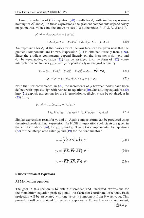
From the solution of (17), equation (20) results for φxe with similar expressions

holding for φye and φz

e . In these expressions, the gradient components depend solelyon geometrical values and the known values of φ at the nodes P, E, S, N, B and T.

φxe · θ = φPE (ySNzBT − yBT zSN)

+ φSN (yBT zPE − yPEzBT) + φBT (yPEzSN − ySNzPE) (20)

An expression for φe at the baricenter of the east face, can be given now that thegradient components are known. Expression (21) is obtained directly from (15a).Since the gradient components depend linearly on the increments φPE, φSN andφBT between nodes, equation (21) can be arranged into the form of (22) whereinterpolation coefficients γE, γN and γT depend solely on the grid geometry.

φe = φP − xPeφxe − yPeφ

ye − zPeφ

ze = φP − −→

Pe · ∇φe (21)

φe = φP + γE · φEP + γN · φNS + γT · φT B (22)

Note that, for convenience, in (22) the increments of φ between nodes have beendefined with opposite sign with respect to equations (20). Substituting equations (20)into (21) explicit expressions for the interpolation coefficients can be obtained, as in(23) for γE.

γE · θ = xPe (ySNzBT − yBT zSN)

+yPe (zSN xBT − zBT xSN) + zPe (xSN yBT − xBT ySN) (23)

Similar expressions result for γN and γT . Again compact forms can be produced usingthe mixed product. Final expressions for FTSE interpolation coefficients are given inthe set of equations (24), for γE, γN and γT . This set is complemented by equations(22) for the interpolated value φe and (19) for the denominator θ .

γE =⟨−→Pe,

−→SN,

−→BT

⟩· θ−1 (24a)

γN =⟨−−→P E,

−→Pe,

−→BT

⟩· θ−1 (24b)

γT =⟨−−→P E,

−→SN,

−→Pe

⟩· θ−1 (24c)

5 Discretization of Equations

5.1 Momentum equation

The goal in this section is to obtain discretized and linearized expressions forthe momentum equation projected onto the Cartesian coordinate directions. Eachprojection will be associated with one velocity component from �v = (u, v, w). Thisprocedure will be explained for the first component u. For each velocity component,


a system of linear equations will be obtained, with one equation for each volumeelement in the grid. The general form of this system will be:

Auu = Qu (25)

where Au is an N × N coefficient matrix, u is the vector of unknowns and Qu theindependent vector term, being N the total number of grid elements. The coefficientmatrix Au is heptadiagonal, corresponding to the seven point computation moleculeof Fig. 1, within each structured grid block. For a single generic element P we have:

AuP · uP + Au

W · uW + AuE · uE + Au

S · uS + AuN · uN + Au

B · uB + AuT · uT = Qu

P (26)

where the coefficients Aui and the source term Qu

P result from the discretization andlinearization of the different terms in equation (2).

Equation (27) presents the approximation of convective u flux terms for a givenvolume element, through the east face (see Fig. 3).

Fcue =

∫Se

ρu(�v · nS

)dS ≈ meue = max (me, 0) uP + min (me, 0) uE

+ γCDS

(meue − max (me, 0) uP − min (me, 0) uE

)

= AcueP · uP + Acue

E · uE − QcueP (27)

The mass flux through the east face (me) participates explicitly in equation (27),allowing the linearization of the convective flux. The computation of mass fluxes willbe considered in the next section when the mass balance equation is analysed. Theapproximation of the convective flux consists of an implicit, first order, upwind termand an explicit deferred correction [2, 10], which is of second order since the linearlyinterpolated velocity component ue at the face center e is used. The interpolationscheme might be a standard CDS scheme or an improved FTSE scheme. The implicitterm in equation (27) contributes to the coefficient matrix Au, while the explicitcorrection adds to the source term Qu. The use of an explicit deferred correctionallows the inclusion of higher order approximations [6, 8], while preserving thesimplicity and robustness of the implicit method.

The approximation of diffusive terms is considered next in equation (28), againfor first Cartesian direction and through the east face:

Fcue =

∫Se

(2μD · nS

) · e1dS =∫

Se

μ (∇u) · nSdS +∫

Se

μ∂�v∂x

· nSdS

≈ μe (uE − uP)

∣∣∣�Se

∣∣∣∣∣∣−−→P E∣∣∣

+(

2μe De · �Se

)· e1 − μe (∇u)e · −−→

P E

∣∣∣�Se

∣∣∣∣∣∣−−→P E∣∣∣

= AdueP · uP + Adue

E · uE − QdueP (28)

The approximation is split into an implicit first order term and an explicit deferredcorrection of higher order. The implicit term considers only the contribution ofthe given velocity component (u) to approximate the diffusive flux. The explicit


correction takes in account the full expression of the interpolated symmetric tensorDe. Similar flux expressions hold for the other volume element faces w, n, s, t, b . Thepressure term in equation (2) is approximated, using Gauss theorem, by the pressuregradient computed as in equation (11):

∫S−pnS · e1dS =

∫�

−∇ · (pe1

)d� ≈ −

(∂p∂x

)P

�� = QpuP (29)

Equation (29) contributes only to the source term Qu. The pressure itself isupdated through the mass balance, as explained in Section 5.2

The remaining terms in equation (2) are given by volume integrals and theirapproximation is simple, through cell centered discretizations:

∫�

ρ∂u∂t

d� ≈ ρ

�t

(uP − uold

P

)�� = Atu

P · uP − QtuP (30)

∫�

ρβ(T − Tref

) �g · e1d� ≈ ρβ(TP − Tref

) �g · e1�� = QguP (31)

In equation (30) a first order backwards approximation was considered for thetime derivative, while higher order terms can be easily considered, introducingmultiple time step schemes.

5.2 Mass balance equation

The velocity field obtained from the discretized approximations to the momentumbalance equation (2) is not subject to the incompressibility condition and thus itmust be corrected to fulfil the mass balance equation (1). An equation to update thepressure field is also needed. With these purposes the SIMPLE method for pressure-velocity coupling [2] is used in this work. The current estimates for the velocity andpressure fields (�v�

, p�) will be modified by adding velocity and pressure corrections(�v′

, p′) to obtain new current estimations (�v, p):

�v = �v� + �v′ p = p� + p′ (32)

The correction fields (�v′, p′) are determined so that the new velocity field (�v) verifies

the mass balance. The relation between the velocity and pressure corrections isinspired in equations (26) and (29):

�v′e = −

(��

AP

)e

(∇ p′)e (33)

Equation (33) reflects that, in an incompressible fluid, the pressure field acts as alink enforcing the incompressibility condition onto the velocity field. Equation (33)neglects the influence of other terms from the momentum balance in equation (26)and thus the resulting new estimations (�v, p) will not fulfil exactly the momentumbalance.


The mass flux through, for example, the east face of a given volume elementcentered in P can be approximated by the interpolated quantities at the facecenter e:

me =∫

Se

ρ(�v · nS

)dS ≈ ρe

(�ve · �Se

)(34)

Using equation (33) expressions for the corrected mass fluxes at each face of avolume element can be obtained. For the east face:

me = m�e + m′

e = ρe

(�v�

e · �Se

)

−(

ρ��

AP

)e

�Se · ((∇ p)e − (∇ p)e

) −(

ρ��

AP

)e

�Se · (∇ p′)e (35)

The first term in the right hand side of equation (35) corresponds to the uncor-rected mass flux m�

e, computed as in (34) using the current estimation of the velocityfield (�v�) obtained from the momentum balance equation. The second term is acorrection to prevent oscillations in the pressure field [10, 13], based on the differencebetween the pressure gradient computed at the face center by central differences andthe interpolated pressure gradient . The third term in the right hand side of equation(35) represents the mass flux correction m′

e, thus accounting for the contribution ofpressure correction (p′) onto the velocity, according to equation (33). This last termproduces the equation for the pressure correction (p′), when the expressions for thecorrected mass fluxes are substituted into the discretized mass balance equation with(∇ p′)

e approximated by central differences.

∑c

mc =∑

c

m�c +

∑c

m′c = 0 (36)

In this way equation (37) for the pressure correction is obtained, with the samestructure as equation (26). This procedure might be adapted to deal with compress-ible flows, by allowing corrections to the density field and relating these correctionsto the pressure corrections through appropriate equations of state [2].

ApP · p′

P + ApW · p′

W + ApE · p′

E + . . . + ApT · p′

T = QpP (37)

5.3 Iteration scheme

Within each time step equations (26) for each component of the velocity andequation (37) for the pressure correction are solved alternately and successively. Inaddition equations for scalar transport, similar to (26) and which will not be detailedhere, are solved. Thus, the solution to the non-linear, coupled, partial differentialequation system (1, 2 and 3) is approximated by the solution of a succession oflinear equation systems, as represented in Fig. 5. The model caffa3d.MB currentlyimplements, for the iterative solution of these linear systems, the methods SIP and


Fig. 5 Iteration scheme forone time step (adaptedfrom [12])

CGStab [2], and an AMG linear solver, that uses SIP as a smoother, presented below.Incorporating other methods for solving linear systems is straightforward.

6 Boundary Conditions and Block Interfaces

6.1 Boundary conditions

Boundary conditions are taken in account through a special treatment of flux terms inequations (1, 2 and 3), for the case of boundary volume elements, as those pictured ifFig. 6. The scheme for neighbours P − E of Fig. 3 is replaced by the scheme P − PBof Fig. 6a. The nodes PB are additional grid nodes placed at the center of boundaryfaces, as shown in Fig. 6b, to simplify the application of boundary conditions. Fieldvalues at these nodes do not participate as unknowns in the linearized systems ofequations for inner nodes.

First, the contribution from inner cells and faces to the coefficients and sourceterms of equations (26) and (37) is considered following the structured arrangementwithin each grid block. Next, an indexed list to the boundary faces, as that of Fig. 6a, islooped through to consider the contribution of each boundary cell to these equations.The model currently implements inlet and outlet boundary conditions as well assymmetry surfaces and walls, both fixed or moving through sliding interfaces. Otherboundary conditions can be incorporated easily.

6.2 Block interfaces

The consideration of block structured grids requires special attention to the volumeelements placed at the interfaces between blocks. In Fig. 7a an example is presented,made of two grid blocks with a matching one-to-one interface. The scheme of Fig. 3must be replaced for the case of block interface cells by the similar scheme of Fig. 7b.

Fig. 6 a Boundary volumeelement. b Grid detail at theboundary

ba


Fig. 7 a A ‘one-to-one’ blockinterface. b Volume element Pat a block interface

a b

The neighbour R belongs now to a different grid block. This is a non structuredrelation between P and R, so the information about block interface relations is storedin an indexed list.

Following the scheme of Fig. 7b, for a volume element P placed at the interfaceof the first block, equation (26) is replaced by equation (38), where the structuredterm Au

E · uE is replaced by the unstructured term AuR · uR, and the coefficient Au

P ismodified correspondingly:

AuP · uP + Au

W · uW + AuR · uR︸︷︷︸

interface

+AuS · uS + . . . + Au

T · uT = QuP (38)

Analogously, equations for interface cells in the second block will incorporatenon structured terms of the form Au

L · uL replacing the structured terms AuW · uW .

The resulting coefficient matrix Au is now block-heptadiagonal with non structuredcoefficients, corresponding to the interfaces between grid blocks, distributed in theoff diagonal blocks of the matrix, as shown in Fig. 8. These off diagonal coefficientsare taken in account to update the residual vector during the linear system iterations,although not to build the iteration matrix. Still the implicit character of the methodis conserved [10]. The volume elements at the interfaces between grid blocks are notboundary nodes, but inner volume elements with special non structured informationabout their neighbour elements. They receive an essentially implicit treatment.

The case of many-to-one block interfaces, as the one shown in Fig. 9, can betreated analogously to that of the matching one-to-one block interface seen above.The relation between volume elements is injective if seen from the nodes P of thefiner block, so that the construction of an indexed list and the consideration of

a b

Fig. 8 Structure of linearized equation system Auu = Qu. a For single block grids matrix isheptadiagonal. b In block structured grids the coefficient matrix becomes block heptadiagonal, with areduced amount of non structured coefficients in off diagonal blocks corresponding to the interfacesbetween blocks


Fig. 9 Sketch of many-to-oneblock interface. The indexedneighbour R inheritscontributions from more thanone ‘P’ node (two in this case:P and P’)

additional coefficients in the linearized system of equations is done in the same way asbefore. In fact the implementation of non-matching many-to-many block interfaces,mostly differs in the increased complexity of building the indexed list of relationshipsthrough the interface and computing the geometrical properties involved. Once thisis done, the process of building the coefficient matrices, and the iterative solutionof the resulting linear systems scarcely require modifications. The case of slidinginterfaces that will be considered next is a particular case of many-to-many nonmatching interface, where the referred process can be simplified.

6.3 Sliding block interfaces

The implementation of sliding block interfaces allows to incorporate moving rigidbodies within the domain, whose movement might be prescribed or can result fromtheir dynamic interaction with the fluid. The precondition for this approach is thatthe interfaces between sliding blocks must keep their shape during the movement.This is appropriate for rotating bodies rather than freely moving ones. On the otherhand the extra computational effort required is minimal, with no need to recomputethe grid at each step, since only some connectivity information needs to be updated.

In Fig. 10 an example of sliding interface between two concentric grid blocks isgiven. The interior block is fixed, while the exterior block rotates. The distribution ofcells in each block matches the other for the case of null relative displacement angleα. For other values of α, any given cell at the interface relates to at most two othercells in the opposite grid block. The indexed list of relationships between cells in theinterface and the influence fractions between cells can be computed explicitly, at anytime step, from the value of the angle α. The geometrical properties of the cells in therotating block can also be updated applying a rotation through simple trigonometricrelations.

To compute coefficients in the discretized of equations (26, 37) the relativemovements of grid blocks must be considered. The local time derivative of the

Fig. 10 Sketch of slidinginterface between twoconcentric blocks, with detailof grid and relativedisplacement angle α


absolute velocity field is computed, for each moving block, in fixed points of therotating system and the relative velocities are used for the mass fluxes. With theseconditions equations (39) and (2) are equivalent:

∫�

ρ∂R�vA

∂td� +

∫Sρ�vA

(�vR · nS

)dS =

∫�

ρβ(T − Tref

) �g · e1d�

+∫

S−pnS · e1dS +

∫S

(2μD · nS

) · e1dS (39)

where the subindex (A) refers to the inertial reference system and the subindex(R) refers to the reference system that rotates with the grid block. The relativemovement between blocks is that of a rigid body. It is thus incompressible whichhas been implicitly considered in (39). Equation (39) is not the expression for themomentum balance equation in a non-inertial reference frame, since it still considersthe absolute momentum (ρ�vA). It is rather the transformation of (2) under theconditions mentioned before.

The iterative solution of the resulting linearized systems require no other mod-ifications than the consideration of additional non-structured coefficients for thecomputation of residual vectors, as in the case of one-to-one block interfaces. Ifthe movement of the rigid parts is not prescribed, additional dynamic equationsfor the involved rigid bodies must be introduced to describe their movement. Anexample considering a simple mixer will be presented in Section 9.3

7 Block Structured AMG Solver

It is well known that the performance of usual linear solvers deteriorates as thenumber of nodes increases, since they only smooth efficiently the high spatialfrequency components of the error, while the lower spatial frequency componentsare decreased much slower. Different multigrid strategies have been proposed todeal with this problem [2, 6, 11]. The common principle is to smooth the lowerspatial frequency components of the error through a succession of coarsened grids[9]. The iterations in the coarser grids are inexpensive since, in three dimensionalcases, the number of points is decreased by eight from one grid level to the next, whilethe number of iterations required in the finest grid is, for the multigrid approach,independent of the number of points. The AMG solver presented next is usuallyonly applied to the pressure equation, since it is usually the hardest to convergefor the linear solver, while the iterations for the momentum equations convergemuch rapidly. In this paper the AMG approach described in [11] was followed,adapting it to work in the block structured grid context presented before. The AMGstrategy works directly with the linear system produced at the original grid. Insteadof explicitly defining a set of coarser grids and building the corresponding linearsystem at each grid, a set of increasingly coarser linear systems is derived directlyfrom the original linear system applying a blocking procedure through the use oftransfer operators [11]. Not needing to explicitly define and compute the propertiesof a series of coarser grids is an advantage when dealing with non-orthogonal, bodyfitted grids, as is the case here. Still, coarser levels l = 2, 3, ..., lmax might be regarded


a b

Fig. 11 a Relation between grid levels. Fine grid in black and coarse grid in gray. Restrictionoperator averages fine grid residuals into coarse grid, while injection operator copies coarse gridcorrections into fine grid. b W-cycle in AMG method

as related to coarser grids obtained by grouping volume elements from the previouslevel in blocks. Figure 11a illustrates this for a schematic grid.

A linear system is defined at each level, with the first, finest, level corresponding tooriginal grid. Coarser levels are constructed to damp the error at increasingly lowerspatial frequencies:

A1x1 = b1 , A2x2 = b2 , ... , Alxl = bl , ... (40)

The coefficient matrices at each coarse level l + 1 are derived from the previousfiner level l by grouping the coefficients through a transfer operator. For the ninepoint scheme in three dimensions, a suitable transfer operation is the following:

AP(i, j,k)l+1 =2i+1∑m=2i

2 j+1∑n=2 j

2k+1∑p=2k

AP(m,n,p)l +2 j+1∑n=2 j

2k+1∑p=2k

AE(2i,n,p)l + AW (2i+1,n,p)l

+2i+1∑m=2i

2k+1∑p=2k

AN(m,2 j,p)l + AS(m,2 j+1,p)l

+2i+1∑m=2i

2 j+1∑n=2 j

AT (m,n,2k)l + AB(m,n,2k+1)l (41a)

AE(i, j,k)l+1 =2 j+1∑n=2 j

2k+1∑p=2k

AE(2i+1,n,p)l (41b)

with expressions similar to (41b) holding for AW , AN, . . . ,AB.


The residual from the solution of the linear system at level l provides theindependent term for the next coarser level l + 1. The restriction operator selectedsimply adds up the residual at each 2 × 2 × 2 block of cells in level l to obtain theindependent term in level l + 1.

rl = bl − Alxl (42a)

rl → restriction → bl+1 (42b)

For any location (i, j, k) in the coarser level l + 1, the result of the restrictionoperation on the residual at the next finer level l is:

b(i, j,k)l+1 =2i+1∑m=2i

2 j+1∑n=2 j

2k+1∑p=2k

r(m,n,p)l (43)

At each level the smoothing of the solution is performed by iterating the linearsystem with an appropriate solver. Here the SIP solver, adapted to work withblock structured grids as described in [10] and to deal with the multilevel indexingassociated with AMG, has been incorporated to work as the smoother. The solutionobtained at a coarser level l + 1 is used to obtain a correction cl for the next finer levell through an injection operation, which simply copies the coarse grid values to eachcorresponding block of 2 × 2 × 2 cells in the fine grid. If xold

l is the existing solutionat level l, and xl+1 is the obtained solution at level l + 1, then the new approximationxl at level l is obtained by:

xl+1 → injection → cl (44)

c(m,n,p)l = x(2i,2 j,2k)l+1 , m=i,i+1 n= j, j+1 p=k,k+1 (45)

xl = xoldl + cl (46)

At the interfaces between grid blocks, the interaction coefficients AR and AL, asfor example in equation (38), are grouped through the same transfer operator usedfor the AE, AW , . . . , AB coefficients. Thus, equations similar to (41b) apply. Iterationsare started at the finest grid and proceed down to the coarsest level. The return pathis done in successive V-cycles as shown in Fig. 11b, to progressively accumulate andsmooth the corrections at each level.

8 Parallelization Using OpenMP

The OpenMP programming model allows parallel computation in shared memorycomputers (SMP) through compilation directives. Although it lacks the flexibility ofthe message passing interface (MPI) framework, since it cannot be applied directly todistributed memory systems, it has advantages in terms of simplicity and performancein SMP systems. The strategy of domain decomposition can be easily adapted to


OpenMP, specially in the case of block structured grids. The data structure designedto support block structured grids gives a natural framework to distribute the workamong the different processors.

8.1 Domain decomposition

The domain decomposition strategy uses the same data structure of the blockstructured grid approach. For every task, each processor is assigned with one or moregrid blocks. Only tasks associated with the interfaces between blocks are done bya single processor, since they potentially involve situations of interfering memoryaccess.

The main advantages of this approach are the programming simplicity, the abilityto control the domain decomposition through the design of the block structured grid,and the high efficiency attained when a good load balance is achieved. As opposed toMPI there is no effort wasted in sharing information between processors, since theyall share the same memory. A significant drawback however is the difficulty to attaina good load balance in some cases, as for example a grid composed of only two blocksof very different size. A workaround is to arbitrary divide the bigger block into twoconveniently sized blocks.

The introduction of OpenMP directives does not require the modification of theserial program structure. This ensures that the results of the computations will be thesame, except for roundoff errors due to the different ordering when doing sums overthe whole domain, for example for the computation of residuals.

8.2 Preliminary analysis of speed up

To evaluate the speed up factor obtained with OpenMP, a two processor SUN FireV20z Server was used. The system runs AMD Opteron 248 processors, with 1 MBcache and 2 GB of RAM. The test case was the lid-driven flow in a cubical cavityat Re = 1000, which is analysed in Section 9.1. The grid was set up with two blocks,with a total of 613 nodes. The speed up factor was of 1.8× with respect to the serialexecution.

The speed up factor is strongly dependent on the architecture of the multi-processor system and on the choice of compiler. Similar results to those reportedabove (1.75×) were obtained in a two processor DELL system with two Intel Xeonprocessors (512KB cache and 1 GB RAM). However, using a generic two processorsystem with two AMD Atholon MP processors (256 KB cache and 1 GB RAM) thespeed up factor was only 1.4×. The limiting factor was detected to be the memoryaccess, due to a poor performance of the data bus, since two independent serialprocesses running simultaneously suffered a similar performance loss.

9 Application Examples and Results

9.1 Cubical lid-driven cavity at Re = 1000

The first application considered is that of the lid-driven flow inside a cubical cavityat Re = 1000. This is a traditional test case for Navier-Stokes solvers, with good


Fig. 12 Sketch of lid-drivencavity. Re = Vo · h/ν = 1000

numerical solutions being available in the bibliography [1, 3, 5] to validate theobtained results. The recent results from [1] will be used here for validation. Figure 12presents a sketch of the domain. Non slip boundary conditions are applied to all walls,with the top one sliding at constant velocity Vo. Given the height h of the cavity andthe lid velocity Vo, the fluid viscosity ν is set so that Re = 1000. The computationswere run until steady state was achieved.

Simulations were run for two series of systematically refined grids, one withuniform distribution of grid points and the other with a finer resolution near the walls.The number of points on each side of the cavity was N = 21, 41, 61, 81, 101, and 121respectively. A reference solution was computed applying Richardson extrapolationto the solutions obtained from the finer stretched grids. Figure 13 presents normal-ized velocity profiles at horizontal and vertical centerlines for uniform grids withN = 41 and 81, and stretched grid with N = 121. Comparison is provided against theresults from spectral computations in [1]. In Table 1 the minimum and maximum

Fig. 13 Horizontal andvertical velocity profiles atcenterlines. Results fromuniform grids with N = 41(dash-dotted line) and N = 81(dashed line), and stretchedgrid with N = 121 (solid line),compared with results from [1](symbols: o)


Table 1 Minimum and maximum velocity components on vertical and horizontal centerlines, fordifferent grid resolutions

Nx × Ny × Nx maxy(v) y miny(v) y minx(v) x

41 × 41 × 41 0.2240 0.1134 −0.3949 0.9101 −0.2530 0.131781 × 81 × 81 0.2404 0.1110 −0.4241 0.9106 −0.2727 0.1267121 × 121 × 121 0.2438 0.1101 −0.4301 0.9101 −0.2769 0.125341 × 41 × 41a 0.2384 0.1110 −0.4311 0.9116 −0.2710 0.127281 × 81 × 81a 0.2445 0.1096 −0.4340 0.9101 −0.2779 0.1249121 × 121 × 121a 0.2457 0.1093 −0.4350 0.9098 −0.2793 0.124596 × 96 × 64b 0.2467 0.1091 −0.4350 0.9096 −0.2804 0.1242

Results given for uniform gridsaStretched gridsbSpectral method computations from [1]

values for the velocity components along the centerlines are presented for selectedgrids, together with the results reported by [1]. Results for the solution on theN = 121 stretched grid are within 0.4% of those in [1]. Also both series of systemat-ically refined grids show monotonic convergence towards these reference values.

The rate of error decay as the uniform and stretched grids are refined was com-puted. The error for the horizontal velocity component along the vertical centerlinefor both set of grids is shown in Fig. 14a. In both cases the error decay fits wellthe expected theoretical decay for a second order method, with the stretched gridperforming better. To validate the FTSE interpolation, a series of block structuredgrids were configured. Three blocks were used, with an outer finer block near thewall interfacing with a coarser middle block and finally an orthogonal block at the

a b

Fig. 14 a Error reduction with grid resolution for orthogonal grids. The error norm for horizontalvelocity at vertical centerline is shown for uniform (�) and stretched (�) grids respectively withN = 21, 41, 61, 81, 101 and 121. Solid line shows expected N−2 decay. b Error reduction with gridresolution in non-orthogonal grid, for CDS (�) and FTSE (�). Solid line show fitting potential decaysN−1.6 and N−2.2 respectively


Fig. 15 a Uniform gridb Non-orthogonal O-type gridused to test the FTSE linearinterpolation scheme. Picturedgrids correspond to N = 21resolution

ba

center as pictured in Fig. 15b. The resulting composite grid is non orthogonal, andalso exhibits sharp changes in grid line direction and sudden grid refinement acrossblock interfaces, providing a challenge for standard CDS interpolation. Simulationsin the O-type grids were run for different resolutions corresponding to N = 21, 41and 81. In Fig. 14b error decay with increasing resolution is given for the O-typegrids, using both the standard CDS and the improved FTSE interpolation schemes.The FTSE scheme preserves true second order error decay, while for CDS it reducesto 1.6.

9.2 Flow inside a PCB enclosure model

The simulation of the flow inside a printed circuit board enclosure is considered next.This study case motivated the development of the code and takes advantage of theblock structured grid approach. Figure 16 presents a sketch of the domain (a), theblock structured grid for this case (b) and an image of the experimental setup forthe time resolved PIV measurements described in [14]. The Reynolds number atthe entrance section was set to Re = U.h/ν = 1.2 × 103. Spatial resolution was setto h/70 near the walls and about h/35 at the core, using stretched grid blocks, for atotal of 3.1 × 106 nodes. This configuration occupies 1 GB RAM and was run on thetwo processor systems mentioned in Section 8.2, under OpenMP. A general view ofthe flow is given in Fig. 17 through the visualization of λ2 iso-surfaces [4]. The upper

a b c

Fig. 16 a Sketch of domain. b Block structured grid. c Experimental setup


Fig. 17 Instantaneous vortexstructures, identified by meansof λ2 iso-surfaces

channel is dominated by two large counter rotating vortical structures, which breakdown at the entrance to the lower channel.

Figures 18 and 19 present streamline patterns in the region indicated in Fig. 16a,at the entrance of the lower channel and beneath the plate, from PIV experimentsand numerical simulations, respectively. In the experimental results a recirculationregion is observed, centered at approximately (y/h = 0.85, x/h = 4.35) and with anhorizontal extension of about h. For the numerical results the recirculation regionis slightly displaced downstream, with center at (y/h = 0.85, x/h = 4.15), and has

Fig. 18 Streamlines forthe mean velocity field in thecentral vertical section at theentrance of the lower channel(see Fig. 16a), from timeresolved PIV


Fig. 19 Same as Fig. 18, butfor numerical results

an horizontal extension of about 1.4h. Also a small recirculation region near thecorner at (y/h = 0.0, z/h = 6.0) barely appears in the experimental results, whileit is clearly defined in the numerical results.

9.3 A simple mixer

The last application has been selected with the purpose of validating the slidinginterface technique described in Section 6.3. The case is that of a simplified mixerwith a single central rotating blade, as sketched in Fig. 20, inside a square container.

The body fitted block structured grid is shown in Fig. 21a). The grid contains fiveblocks. Two outer grid blocks (cyan and magenta) that are fixed and three inner gridblocks (red, blue and green) that rotate with the blade. The sliding interface existsbetween cyan and green blocks. The red block is an incomplete cylinder, while theblue block provides a simple representation of the blade geometry. The shape, sizeand number of blades could be easily modified by changing these two blocks or bydecomposing them into several smaller blocks.

The fluid and blade are initially at rest, and a passive scalar profile is specified asshown in Fig. 21b in order to visualize the flow. The initial profile of this tracer hasbeen slightly smeared in order to prevent oscillations due to a sharp edge. Non slipboundary conditions were applied to all vertical surfaces for the outer container andthe blade, with their respective velocities. Symmetry boundary conditions hold ontop and bottom surfaces, so the flow is essentially planar. The blade starts movingabruptly with angular velocity ω. The Reynolds number is Re=ωL2/ν =500, being

Fig. 20 Simplified mixer, witha single rotating central bladein a square container


Fig. 21 a Block structuredgrid for the simplified mixersimulation. b–f Time evolutionof passive scalar field (φ)through the first revolution ofthe blade and at the end of thesecond revolution (f). The thinblack line is the iso-curve ofφ = 0.5 a b c

d e f

L the length of the blade. The remaining frames in Fig. 21 show the evolution duringthe first revolution of the blade (Fig. 21b–e) and after two revolutions (Fig. 21f). Theiso-curve of φ = 0.5 shows no singularities across the domain or block interfaces.There is no appreciable distortion due to the sliding interface.

Several simulations were run with different time step lengths to verify secondorder accuracy in time for a non stationary case with time dependent boundaryconditions. Results for error decay with time step length are given in Fig. 22. Thefirst two points correspond to time steps for which the blade rotates more than onegrid block per time step. For smaller time steps truly second order decay is achieved.

Fig. 22 Error reduction withtime step. Error norm forscalar field φ is shown. Solidline shows expected theoreticaldt−2 decay


10 Conclusions

An implementation of the finite volume method in block structured body fittedgrids has been presented, for the simulation of three dimensional flows. The decom-position of the global grid into structured grid blocks allows to incorporate someadvanced features. Qualitative as well as quantitative results for some applicationswere obtained that demonstrate these capabilities, as for example the incorporationof moving rigid bodies through sliding interfaces and the parallel computationthrough domain decomposition using OpenMP. Preliminary results show that theperformance increase under OpenMP is dependant of specific hardware implemen-tations, presumably those regarding the speed of memory access. Also, an AMGsolver was incorporated and adapted to work under the block structured grid frame-work. An improved linear interpolation scheme for non-orthogonal grids, based onmultidimensional Taylor series expansions, was shown to preserve the second orderbehaviour of the method, while the performance with a standard CDS interpolationin non-orthogonal grids deteriorates. Second order accuracy in time has also beenverified. The numerical model presented here has been made freely available,to promote cooperative developments in the field. For turbulent flows, LES andκ-ε models are available, while a free surface module integrated to caffa3d.MB iscurrently being validated and will also be made available shortly.

Acknowledgements This work was supported by FPI/DPI2003-06725-C02-01 and DPI2006-02477from DGI, Ministerio de Educación y Cultura y Fondos FEDER, Spain, and grants 33/07, 48/01 PDTand I+D CSIC, Uruguay. The authors are grateful to Dr. Milovan Peric for his authorization to usethe 2D numerical model caffa as a basis to develop caffa3d.MB.

References

1. Albensoeder, S., Kuhlmann, H.C.: Accurate three-dimensional lid-driven cavity flow. J. Comput.Phys. 206, 536–558 (2005)

2. Ferziger, J., Peric, M.: Computational Methods for Fluid Dynamics. Springer, Berlin (2002)3. Iwatsu, R., Hyun, J.M., Kuwahara, K.: Analyses of three dimensional flow calculations in a driven

cavity. Fluid Dyn. Res. 6(2), 91–102 (1990)4. Jeong, J., Hussain, F.: On the identification of a vortex. J. Fluid Mech. 285, 69–94 (1995)5. Jiménez, A.: Interaccio entre les estructures de flux i el transport de materia. Aplicacio a un doll

pla turbulent. Ph.D. thesis, URV (2003)6. Lange, C.F., Schäfer, M., Durst, F.: Local block refinement with a multigrid solver. Int. J. Numer.

Methods Fluids 38, 21–41 (2002)7. Lehnhauser, T., Schäfer, M.: Improved linear interpolation practice for finite-volume schemes

on complex grids. Int. J. Numer. Methods Fluids 38, 625–645 (2002)8. Lehnhauser, T., Schäfer, M.: Efficient discretization of pressure-correction equations on non-

orthogonal grids. Int. J. Numer. Methods Fluids 42, 211–231 (2003)9. Lehnhauser, T., Ertem-Muller, S., Schafer, M., Janicka, J.: Advances in numerical methods for

simulating turbulent flows. Prog. Comput. Fluid Dyn. 4(3–5), 208–228 (2004)10. Lilek, Z., Muzaferija, S., Peric, M., Seidl, V.: An implicit finite-volume method using nonmatch-

ing blocks of structured grid. Numer. Heat Transf. B 32, 385–401 (1997)11. Mora Acosta, J.: Numerical algorithms for three dimensional computational fluid dynamic prob-

lems. Ph.D. thesis, UPC (2001)12. Peric, M.: Numerical methods for computing turbulent flows. Course notes (2001)


13. Rhie, C.M., Chow, W.L.: A numerical study of the turbulent flow past an isolated airfoil withtrailing edge separation. AIAA J. 21, 1525–1532 (1983)

14. Usera, G., Vernet, A., Ferré, J.A.: Use of time resolved PIV for validating LES/DNS of theturbulent flow within a PCB enclosure model. Flow Turbul. Combust. 77, 77–95 (2006)

15. Zaleski, S.: Science and fluid dynamics should have more open sources. http://www.lmm.jussieu.fr/∼zaleski/OpenCFD.html (2001)

http://www.lmm.jussieu.fr/~zaleski/OpenCFD.html

http://www.lmm.jussieu.fr/~zaleski/OpenCFD.html

A Parallel Block-Structured Finite Volume Method for Flows in Complex Geometry with Sliding...

Documents

Transcript of A Parallel Block-Structured Finite Volume Method for Flows in Complex Geometry with Sliding...