Sliding interfaces with contact-impact in large-scale Lagrangian computations
31
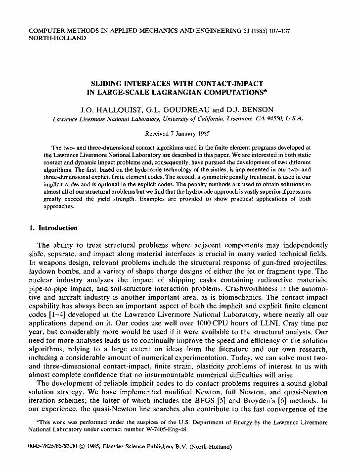
COMPUTER METHODS IN APPLIED MECHANICS AND ENGINEERING 51 (1985) 107-137 NORTH-HOLLAND SLIDING INTERFACES WITH CONTACT-IMPACT IN LARGE-SCALE LAGRANGIAN COMPUTATIONS* J.O. HALLQUIST, G.L. GOUDREAU and D.J. BENSON Lawrence Livermore National Laboratory, University of California, Livermore, CA 94550, U.S.A. Received 7 January 1985 The two- and three-dimensional contact algorithms used in the finite element programs developed at the Lawrence Livermore National Laboratory are described in this paper. We are interested in both static contact and dynamic impact problems and, consequently, have pursued the development of two different algorithms. The first, based on the hydrocode technology of the sixties, is implemented in our two- and three-dimensional explicit finite element codes. The second, a symmetric penalty treatment, is used in our implicit codes and is optional in the explicit codes. The penalty methods are used to obtain solutions to almost all of our structural problems but we find that the hydrocode approach is vastly superior if pressures greatly exceed the yield strength. Examples are provided to show practical applications of both approaches. 1. Introduction The ability to treat structural problems where adjacent components may independently slide, separate, and impact along material interfaces is crucial in many varied technical fields. In weapons design, relevant problems include the structural response of gun-fired projectiles, laydown bombs, and a variety of shape charge designs of either the jet or fragment type. The nuclear industry analyzes the impact of shipping casks containing radioactive materials, pipe-to-pipe impact, and soil-structure interaction problems. Crashworthiness in the automo- tive and aircraft industry is another important area, as is biomechanics. The contact-impact capability has always been an important aspect of both the implicit and explicit finite element codes [l-4] developed at the Lawrence Livermore National Laboratory, where nearly all our applications depend on it. Our codes use well over 1000 CPU hours of LLNL Cray time per year, but considerably more would be used if it were available to the structural analysts. Our need for more analyses leads us to continually improve the speed and efficiency of the solution algorithms, relying to a large extent on ideas from the literature and our own research, including a considerable amount of numerical experimentation. Today, we can solve most two- and three-dimensional contact-impact, finite strain, plasticity problems of interest to us with almost complete confidence that no insurmountable numerical difficulties will arise. The development of reliable implicit codes to do contact problems requires a sound global solution strategy. We have implemented modified Newton, full Newton, and quasi-Newton iteration schemes; the latter of which includes the BFGS [5] and Broyden’s [6] methods. In our experience, the quasi-Newton line searches also contribute to the fast convergence of the *This work was performed under the auspices of the U.S. Department of Energy by the Lawrence Livermore National Laboratory under contract number W-7405Eng-48. 0045-7825/85/$3.30 @ 1985, Elsevier Science Publishers B.V. (North-Holland)
-
Upload
independent -
Category
Documents
-
view
1 -
download
0
Transcript of Sliding interfaces with contact-impact in large-scale Lagrangian computations
COMPUTER METHODS IN APPLIED MECHANICS AND ENGINEERING 51 (1985) 107-137 NORTH-HOLLAND
SLIDING INTERFACES WITH CONTACT-IMPACT IN LARGE-SCALE LAGRANGIAN COMPUTATIONS*
J.O. HALLQUIST, G.L. GOUDREAU and D.J. BENSON Lawrence Livermore National Laboratory, University of California, Livermore, CA 94550, U.S.A.
Received 7 January 1985
The two- and three-dimensional contact algorithms used in the finite element programs developed at the Lawrence Livermore National Laboratory are described in this paper. We are interested in both static contact and dynamic impact problems and, consequently, have pursued the development of two different algorithms. The first, based on the hydrocode technology of the sixties, is implemented in our two- and three-dimensional explicit finite element codes. The second, a symmetric penalty treatment, is used in our implicit codes and is optional in the explicit codes. The penalty methods are used to obtain solutions to almost all of our structural problems but we find that the hydrocode approach is vastly superior if pressures greatly exceed the yield strength. Examples are provided to show practical applications of both approaches.
1. Introduction
The ability to treat structural problems where adjacent components may independently slide, separate, and impact along material interfaces is crucial in many varied technical fields. In weapons design, relevant problems include the structural response of gun-fired projectiles, laydown bombs, and a variety of shape charge designs of either the jet or fragment type. The nuclear industry analyzes the impact of shipping casks containing radioactive materials, pipe-to-pipe impact, and soil-structure interaction problems. Crashworthiness in the automo- tive and aircraft industry is another important area, as is biomechanics. The contact-impact capability has always been an important aspect of both the implicit and explicit finite element codes [l-4] developed at the Lawrence Livermore National Laboratory, where nearly all our applications depend on it. Our codes use well over 1000 CPU hours of LLNL Cray time per year, but considerably more would be used if it were available to the structural analysts. Our need for more analyses leads us to continually improve the speed and efficiency of the solution algorithms, relying to a large extent on ideas from the literature and our own research, including a considerable amount of numerical experimentation. Today, we can solve most two- and three-dimensional contact-impact, finite strain, plasticity problems of interest to us with almost complete confidence that no insurmountable numerical difficulties will arise.
The development of reliable implicit codes to do contact problems requires a sound global solution strategy. We have implemented modified Newton, full Newton, and quasi-Newton iteration schemes; the latter of which includes the BFGS [5] and Broyden’s [6] methods. In our experience, the quasi-Newton line searches also contribute to the fast convergence of the
*This work was performed under the auspices of the U.S. Department of Energy by the Lawrence Livermore National Laboratory under contract number W-7405Eng-48.
0045-7825/85/$3.30 @ 1985, Elsevier Science Publishers B.V. (North-Holland)
108 J.O. Hallquist et al., Sliding interfaces with contact-impact
modified and full Newton schemes. In three dimensions, we have ruled out full Newton as a viable option due to the extreme expense of reforming and factoring a large stiffness matrix for each iteration. We now regularly use quasi-Newton methods with frequent reformations of the stiffness matrix. By optimally coding and fully vectorizing the stress divergence, the expense of equilibrium iterations including line search has been minimized.
Explicit hydrocodes use the viscosity method [7] to resolve the details of shock wave propagation through the mesh with small time-step sizes dictated by the Courant stability limit. In three dimensions, our typical applications use 20 000 elements, 10 000 to 100 000 time steps, with 20 to 30 percent of the nodal points contained in the contact surface definitions. Efficient, cheap algorithms are needed to make such problems affordable. We use primitive elements (one stress point hexahedrons), control the zero energy modes by the simplest possible hourglass control [S], and have an efficient and reliable contact-impact algorithm. With faster and larger computers than presently available, we would quickly expand our three-dimensional analyses to a point where the resolution is roughly equivalent to our two-dimensional counterparts, i.e., by a factor of 10 to 50; therefore the need for efficient algorithms will continue for some time.
In developing general-purpose contact algorithms for three-dimensional solutions, we quickly realized that the rigorous extension of the two-dimensional hydrocode algorithms though feasible, would be too costly. Our earlier experience has shown that Lagrange multiplier methods [9, lo] did not necessarily preserve a smooth force distribution across interfaces. The lack of a smooth force field excited the zero energy modes in the primitive elements in nearly all the contact-impact problems we solved. Furthermore, these modes usually stopped explosive-metal interaction computations, a major application for two-dimen- sional hydrocodes, early in the solution. Thus, we were left with the penalty method as the method of choice. We use the penalty approach in our two- and three-dimensional implicit and explicit codes, but, because it is not always suitable for applications involving high explosives, we retain an approach in our explicit codes that is based in part on the hydrocode methodology developed several decades ago.
In the development which follows, we shall first discuss the hydrocode slideline methodology developed in the 60’s. Our DYNA2D algorithm, based on this work, has been extended to include impact and separation along the slideline. We also implemented this methodology in three dimensions but without the DYNA2D extensions. In Section 3, we discuss the penalty method. In the last section, we present a few applications.
2. Hydrocode methodology
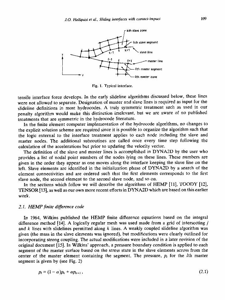
In two dimensions, the contact surfaces along a slideline appear as lines in the y-z plane where y is the horizontal axis, and z is the vertical axis and the axis of revolution in axisymmetric problems. These lines will be referred to as the master and slave lines, respectively. Nodal points along the slave and master lines will be referred to as slave and master nodes, respectively. Likewise, line segments joining adjacent slave and master nodes will be called slave and master segments. Elements that have at least one side that is a slave segment are called slave elements, and master elements are similarly defined. Fig. 1 shows a typical interface. Slave nodes are constrained to slide on or close to the master line unless a
J.U. Haiiquist et al., Sliding interfaces with contact-impact 109
,- kth slave zone
kth slave segment
Pth master segment
Qth master zone
Fig. 1, Typical interface.
tensile interface force develops. In the early slideline algorithms discussed below, these lines were not &wed to separate, Designation of master and slave lines is required as input for the slideline definitions in most hydrocodes. A truly symmetric treatment such as used in our penalty algorithm would make this distinction irrelevant, but we are aware of no published treatments that are symmetric in the hydrocode literature.
In the finite element computer implementation of the hydrocode algorithms, no changes to the explicit solution scheme are required since it is possible to organize the algorithm such that the logic external to the interface treatment applies to each node including the slave and master nodes. The additional subroutines are called once every time step following the calculation of the accelerations but prior to updating the velocity vector.
The definition of the slave and master lines is accomplished in DYNAZD by the user who provides a list of nodal point numbers of the nodes lying on these lines. These numbers are given in the order they appear as one moves along the interface keeping the slave line on the left. Slave elements are identified in the initialization phase of DYNA2D by a search of the element connectivities and are ordered such that the first elements corresponds to the first slave node, the second element to the second slave node, and so on.
In the sections which follow we will describe the algorithms of HEMP fll], TOODY [12], TENSOR [13], as well as our own more recent efforts in DYNA2D which are based on this earlier work.
2.1. HEMP finite difference code
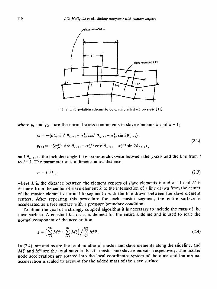
In 1964, Wilkins published the HEMP finite difference equations based on the integral difference method [14]. A logically regular mesh was used made from a grid of intersecting j and k lines with slidelines permitted along k lines. A weakly coupled slideline algorithm was given (the mass in the slave elements was ignored), but modifications were clearly outlined for incorporating strong coupling. The actual modifications were included in a later revision of the original document [15]. In Wilkins’ approach, a pressure boundary condition is applied to each segment of the master surface based on the stress state in the slave elements across from the center of the master element containing the segment. The pressure, pl for the Ith master segment is given by (see Fig. 2)
110 J.O. Huliquist et al., Sliding interfaces with contact-impact
/
slave element k
Fig. 2. Interpolation scheme to determine interface pressure [ 111.
where pk and &+I are the normal stress components in slave elements k and k + 1;
and 6,,,+, is the included angle taken counterclockwise between the y-axis and the line from 1
to I+ 1. The parameter LY is a dimensionless distance,
ff = L’/L, (2.3)
where L is the distance between the element centers of slave elements k and k + 1 and 1;’ is distance from the center of slave element k to the intersection of a line drawn from the center of the master element 1 normal to segment 1 with the line drawn between the slave element centers. After repeating this procedure for each master segment, the entire surface is accelerated as a free surface with a pressure boundary condition.
To attain the goal of a strongly coupled algorithm it is necessary to in&de the mass of the slave surface. A constant factor, z, is defined for the entire slideline and is used to scale the normal component of the acceleration,
*=(~M~+$w;)/~Mp.
i= 1 i=l i=l
(2.4)
In (2.4), nm and ns are the total number of master and slave elements along the slideline, and My and A47 are the total mass in the ith master and slave elements, respectively. The master node accelerations are rotated into the local coordinates system of the node and the normal acceleration is scaled to account for the added mass of the slave surface,
J.O. Hallquist et al., Sliding interfaces with contact-impact 111
1 a n+l _ - - 0,
2 i’f cos @,_,+,+r - j;: sin 81_1,t+1), (2Sa)
as, n+’ = j;t cos 19~-~,,+, + i’l sin 6),_l,lc, . (2.5b)
In the local coordinate system, the normal direction at point I is perpendicular to a line drawn from I- 1 to 1+ 1. The superscript, +, signifies that acceleration has been updated for the pressure distribution. The global accelerations are calculated by rotating the scaled ac- celeration vector back to the global frame,
(2.6a)
-n+1 _ zl -a,, n+l cos e,_,,,+, + a:,+' sin 6,_,,,+, . (2&b)
The final step is the update of the motion of the slave surface. Each slave node k is moved tangentially, treating the master surface as a symmetry plane in the configuration at time iz. The slave nodes are projected back on to the master surface, after the surface is updated into the n + 1 configuration, along the i line on the slave side that contins the kth slave node. Velocities for the slave nodes are then found by dividing the change in coordinates by the time-step size,
Y .n+1/2 = (y+l _ yn)/&“+1/2, jn+1f2 _ - (Zn+’ - ~n)/A~“+‘fz I (2.7)
In early versions of HEMP, the constant z-factor of (2.4) was used rather than a spatially (i) dependent factor. Of course, the assumption of a constant mass distribution is not generally valid and this was acknowledged by Wilkins. Another approximation involved the com- putation of interface pressure from (2.1) and (2.2) where only two slave elements in the immediate vicinity of the mass segment are considered whereas a weighted average of all contiguous slave elements would give a more realistic representation of pI. Also, the pressure normal to the master segment defined by rotating the planar stress is valid only in plane strain in constant Jacobian elements. Ignoring the geometry of the element and the effects.of hoop stress on p/ can lead to values that are too high or low. The methodology of TOODY and TENSOR discussed below overcomes these weaknesses.
2.2. TOODY finite diference
In the TOODY implementation of sliding interfaces, Bertholf and Benzley applied the integral difference method to each master node along the sliding interface. During each cycle a new mesh is defined overlaying the slave elements and matching the mesh density of the contiguous master surface. We shall briefly outline our implementation of the TOODY algorithm in DYNA2D.
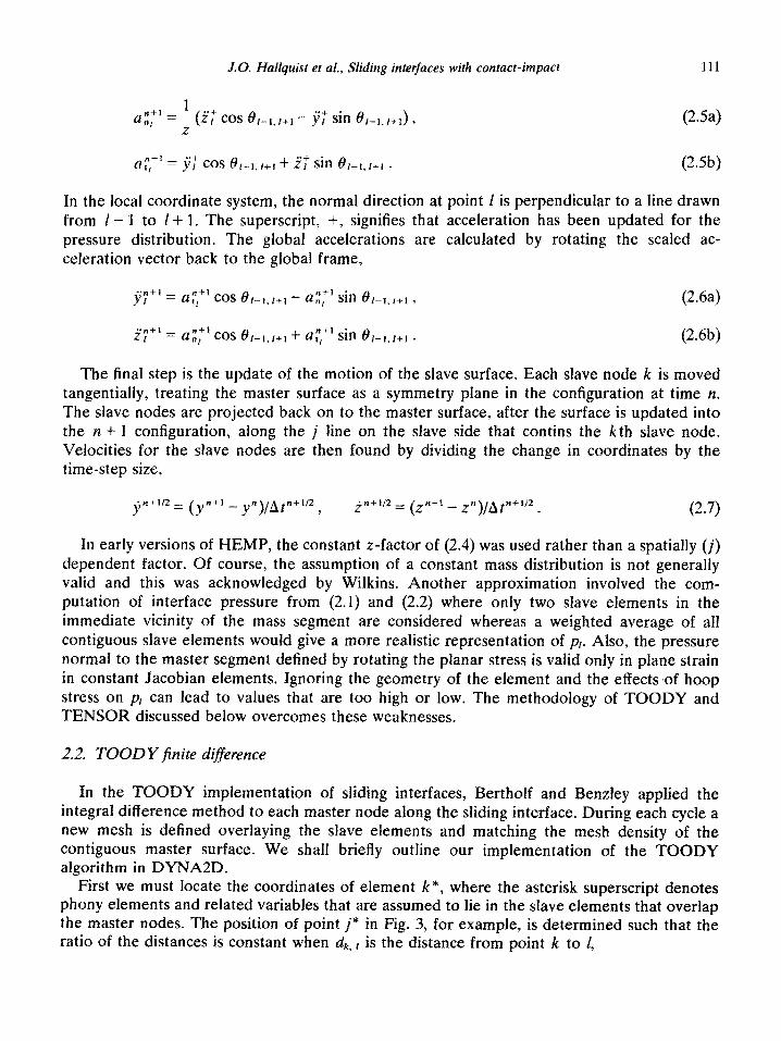
First we must locate the coordinates of element k*, where the asterisk superscript denotes phony elements and related variables that are assumed to lie in the slave elements that overlap the master nodes. The position of point i* in Fig. 3, for example, is determined such that the ratio of the distances is constant when d k. t is the distance from point k to 1,
112 J.O. Hallquist et al., Sliding interfaces with contact-impact
slave element k
phony elementk"
,, j+l j+2 i+l* j+3
CL Te I I
Fig. 3. A typical master segment where slave elements k, k + 1 and k -t 2 contribute to the pressure load applied to
master segment 1. Phony element k* is indicated by dashed lines.
(2.8)
The stresses in the newly defined slave elements are based on a length-weighted inter- polation along the master surface. Consider Fig. 3 where slave element k is the first element to overlap master segment 1 and underlie the phony element k*. Letting S, denote the length of the master segment 1, rtl denote the unit vector tangent to segment I, and Y/,~ denote the vector drawn from 1 to slave node k, we can define S,k for each slave node:
(2.9a)
(2.9b)
(2.9~) /.k+l =
s if r 1. k+l * n/ 9 s, . (2.9d)
The stress contribution to slave element k* made by the stress in slave element k, a:, is designated a$Ik and defined by
d:k = (s, k+, - &,)a#. (2.10)
If inequality (2.9d) is satisfied, u:Ik determines the stress in phony element k*; otherwise, the contribution to the stress tensor of the next overlapped slave element is added. For example, consider the contribution of zone k + 1 to the phony k* zone,
S Lk+2= i
rl. k+2 ’ nl if r I, k+2 * n/ < sl, (2.11a)
s if r l.k+Z’n/’ ’ s ; (2.1 lb)
k’ cij.k+l = (S,,k+2 - &k+l)~:+l/& . (2.12)
If (2.11b) is unsatisfied, k again is incremented by 1, and the procedure given by (2.11)-(2.12) continues until (2.11b) is satisfied. The stress tensor for k* becomes
J.O. Ha&u& et al., Sliding interfaces with contact-impact 113
n-l
OF = C (T$yk+i + (2.13) i=o
where n is the number of overlapping elements. After repeating this procedure to determine the bulk viscosity qk* and density pk., we proceed to the next phony element, k + l*, and
repeat the procedure. We enter the slideline logic in DYNA2D after computing the nodal forces, and therefore
the free surface accelerations of the slave and master nodes are available by dividing the nodal forces by the nodal masses. The tangential accelerations of the master nodes are calculated as if they are free surface nodes, by using (2.5b). For the normal acceleration, the master node is temporarily treated as an interior node surrounded by the master elements and the phony slave elements. A new acceleration (j;:, i’f) is computed, and substituted into (2.5a) with z = 1. The modi~ed global acceleration is calculated from a:+’ and a,“:’ by using (2.6).
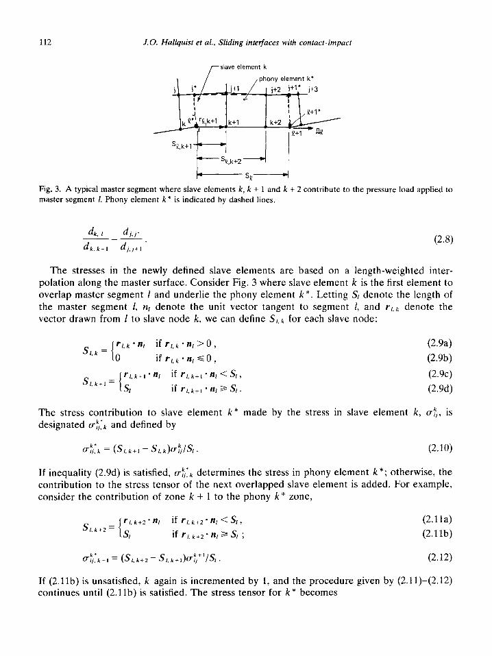
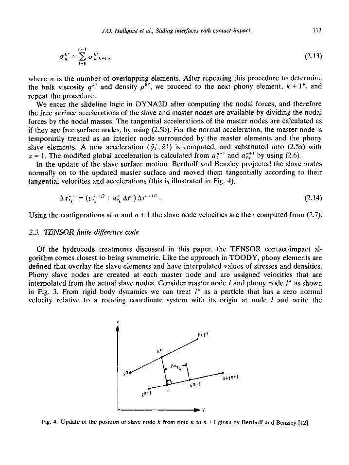
In the update of the slave surface motion, Bertholf and Benzley projected the slave nodes normally on to the updated master surface and moved them tangentially according to their tangential velocities and accelerations (this is illustrated in Fig. 4),
n+l _ Axf, - (u::‘“i- a;, At”) Atn+lf2. (2.14)
Using the configurations at II and n + 1 the slave node velocities are then computed from (2.7).
2.3. TENSOR finite difference code
Of the hydrocode treatments discussed in this paper, the TENSOR contact-impact al- gorithm comes closest to being symmetric. Like the approach in TOODY, phony elements are defined that overlay the slave elements and have interpolated values of stresses and densities. Phony slave nodes are created at each master node and are assigned velocities that are interpolated from the actual slave nodes. Consider master node I and phony node I* as shown in Fig, 3. From rigid body dynamics we can treat E” as a particle that has a zero normal velocity relative to a rotating coordinate system with its origin at node E and write the
P+l”
k” /
Fig. 4. Update of the position of slave node k from time n to n + 1 given by Bertholf and Benzley 1121.
114 J.O. Hallquist et al., Sliding inte#aces with contact-impact
constraint equation for the normal acceleration,
a “I* = a,,+ a,, UC = 2W[(3r* - j,) cOs B,-1, I+I + (.i$ - i,) sin @,_,,,+,I . (2.15)
The normal direction at node 1 is perpendicular to a line drawn from nodes I- 1 to I+ 1, a, is the Coriohs acceleration term, and wi is the angular velocity at node 1,
(‘%+I - i,-I) cos er-*.1+1- tj1+1 - j,-J sin h, 1+1 WI =
d,-I,,+, (2.16)
The expressions for the normal accelerations in terms of an interface pressure p with (2.15) and (2.16) are sotved for p,
a,, = (fn, - ~pcr)h 9
a “,‘ = (f”,. + &w)/m* ,
(2.17a)
(2.17b)
cl = (a+1 - .2,-d sin f3i-1,1+1 + (Y&l - yr-1) cm 81-L i+1 + (2.18)
Here, M, and Ml* are the lumped masses, and fn, and f,,,, are the normal components of the nodal forces at nodes I and I* due to the internaf stress states.
Equation (2.17a) permits the normal acceleration of the master surface to be updated. This procedure is’ repeated for each master node. Since the tangential component of the ac- celeration is unchanged, the global components can be found from (2.6).
Unlike the HEMP and TOODY schemes, where the slave node is moved with the master surface, the TENSOR scheme repeats the foregoing process creating phony nodes and elements on the master side to accelerate the slave surface. After the geometry is updated, slave nodes that do not lie on the master surface are projected normally to the surface. Normal components of velocity are then reset by interpolating from the master side.
2.4. DYNAZL’I finite Everett code
The implementation in DYNA2D will be discussed in detail. Ideas from HEMP, TOODY and TENSOR underlie the current DYNA2D algorithm. Although we feel that the TENSOR scheme may be superior on some problems, it is considerably more expensive and is not easily extended to handie impact problems.
Our current interface treatment may be outlined as follows:
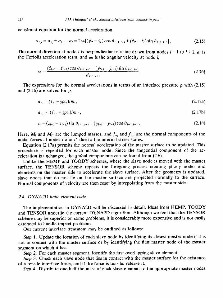
Step 1. Update the location of each slave node by identifying its closest master node if it is not in contact with the master surface or by identifying the first master node of the master segment on which it lies.
Step 2. For each master segment, identify the first overlapping slave element. Step 3. Check each slave node that lies in contact with the master surface for the existence
of a tensile interface force, and if the force is tensile, reIease it. Step 4. Distribute one-half the mass of each slave element to the appropriate master nodes
J.O. Hallquist et al., Sliding interfaces with contact-impact 115
if both slave nodes of the slave segment associated with the element are in contact. If neither of these slave nodes are in contact, distribute no mass. If one slave node is in contact, distribute one-half the mass lying between the contacting node and the center of the slave segment of the slave element.
Step 5. Whenever a slave node reaches the master surface, apply the interface conditions to determine the post-impact velocity.
Step 6. From the states of stress in the slave elements, compute a distributed pressure for each master segment and the equivalent nodal forces. A slave element must be in contact with the master surface to contribute force.
Step 7. For each slave node in contact with a master segment, compute its tangential velocity and acceleration. Interpolate the normal components of velocity and acceleration from the adjacent master nodes.
Step 8. For slave nodes not in contact with the master surface check for penetration during the next time step and reduce the time-step size if necessary so that no slave node penetrates,
The above steps are explained in Sections 2.4.1-2.4.9 in more detail. A typical interface is assumed to consist of n2, slave nodes, II, - 1 slave elements, and n, master nodes. An assumption is made that the master line is sufficiently long so that slave nodes in contact with the line will not slide off the end of the line. In practice, master line extensions are used to ensure that this is the case or, if the user prefers, the slave nodes that slide off can be treated as free surface nodes. If more than one interface exists, the procedures outlined here are repeated from each interface.
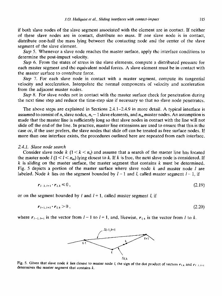
2.4.1. Slave node search Consider slave node k (1 < k < n,) and assume that a search of the master line has located
the master node I (1 < l< n,) lying closest to k. If k is free, the next slave node is considered. If k is sliding on the master surface, the master segment that contains k must be determined. Fig. 5 depicts a portion of the master surface where slave node k and master node 1 are labeled. Node k lies on the segment bounded by I- 1 and 1, called master segment 1 - 1, if
or on the
r/-l, /+l ’ f-1, k d 0 ,
segment bounded by 1 and I+ 1, called master segment I, if
(2.19)
r/-1.1+1 ‘rl,k>O, (2.20)
where rr-l,r+l is the vector from l- 1 to 1+ 1, and, likewise, rl,k is the vector from 1 to k.
/ 9-I ,!2+1
2 Fig. 5. Given that slave node k lies closest to master node I, the sign of the dot product of vectors rck and T,-,,,+, determines the master segment that contains k.
116 J.O. Haliquist et al., Sliding interfaces with contact-impact
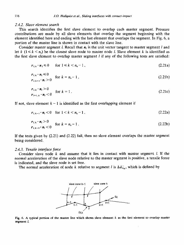
2.4.2. Slave element search This search identifies the first slave element to overlap each master segment. Pressure
contributions are made by all slave elements that overlap the segment beginning with the element identified here and ending with the last element that overlaps the segment. In Fig. 6, a portion of the master line is shown in contact with the slave line.
Consider master segment 1. Recall that nl is the unit vector tangent to master segment 1 and let k (1 G k < n,) be the closest slave node to master node 1. Slave element k is identified as the fn-st slave element to overlap master segment 1 if any of the following tests are satisfied:
r{,k-nI<o for lsk<n,--1, (2.21a)
r/+l.k’%<”
for k = 1 .
(2.21b)
(2.21c)
If not, slave element k - 1 is identified as the first overlapping element if
r,,k_,*n,<O for l<k<n,--1, (2.22a)
rl.k’&>o rIqk-l’& <o
fork=n,-1. (2.22b)
If the tests given by (2.21) and (2.22) fail, then no slave element overlaps the master segment being considered.
2.4.3. Tensile inte~ace force Consider slave node k and assume that it lies in contact with master segment 1. If the
normal acceleration of the slave node relative to the master segment is positive, a tensile force is indicated, and the slave node is set free.
The normal acceleration of node k relative to segment 1 is hii;,,, which is defined by
slave zone k-l slave zone k
Fig. 6. A typical portion of the master line which shows slave element k as the first element to overlap master segment 1.
J.O. Hallquist et al., Sliding interfaces with contact-impact 117
Aii,,, = ii,, - (1 - a&,, - c@i;,+, . (2.23)
The local coordinate (Ye is defined by
ffk = n/ - rlk/hl ’ rl, 1+ I> . (2.24)
If (Yk < E or if (Yk > 1 - E, where E is a tolerance typically in the range of 0.005, the angle 0,_,,,+, or 0,,1+2 is used in place e,,,+, determine the normal in (2.23). The right superscript, -, on nodal quantities denotes the values of the quantities before interface coupling is taken into account.
2.4.4. Addition of slave mass to master mass The mass of the slave elements along the master surface is attributed to the appropriate
master nodes. Each slave element is considered separately. Consider the kth slave element. The mass to be distributed is given by
mk = $kAk (2.25)
for plane strain. For axisymmetric problems, the DYNA2D Petrov-Galerkin scheme is used and, in the above equations, Pk and Ak are the density and are of the kth slave element in the current configuration.
As indicated previously, the kth slave element corresponds to the kth slave node. The kth slave node is being tracked by the master node 1 and is, therefore, known to lie on master segment 1 bounded by master nodes 1 and 1+ 1. Let
Lk. I =
Sk,l’nk if Sk,,‘& >O,
0 if s k,l’nk aO,
(2.26)
where sk, I is the vector from the kth slave node to the center of master segment 1, and nk is the unit vector tangent to the slave segment k bounded by slave
nk = rk, k+l/lrk,k+l I*
Let Lk denote the length Of Slave segment k, i.e., Lk master node 1 from slave element k, mk,,, is given by
(Lk. I/Lk)mk if Lk > Lk, I ,
mk.1’
mk if Lk <Lk,I.
nodes k and-k + 1,
(2.27)
= nk * rk.k+l. The mass attributed to
(2.28a)
(2.28b)
If inequality (2.28b) is satisfied, the next slave element is considered; otherwise, let
L I
Sk,I+l ’ nk if s k. I+1 - nk < Lk , k, /+I =
(2.29a)
Lk if s k.l+l’nk >Lk, (2.29b)
where Sk,l+l is the vector from the kth slave node to the center of master segment I + 1. The
118 1.0. Hall~u~~t et al., Sliding inte~ace~ with
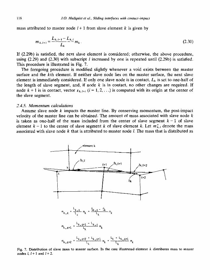
mass attributed to master node I + 1 from slave element k
L k, I+1 - Lk, 1
mk.l+l =
Lk
mk .
is given by
(2.30)
If (2.29b) is satisfied, the next slave element is considered; otherwise, the above procedure, using (2.29) and (2.30) with subscript I increased by one is repeated until (2.29b} is satisfied. This procedure is illustrated in Fig. 7.
The foregoing procedure is modified slightly whenever a void exists between the master surface and the kth element. If neither slave node lies on the master surface, the next slave element is immediately considered. If only one slave node is in contact, Lk is set to one-half of the length of slave segment, and, if node k is in contact, no other changes are required. If node k + 1 is in contact, vector s~,~+~ (i = 1,2,. , .) is computed with its origin at the center of the slave segment.
Assume slave node k impacts the master line. By conserving momentum, the post-impact velocity of the master line can be obtained. The amount of mass associated with slave node k is taken as one-half of the mass included from the center of slave segment k - 1 of slave element k - 1 to the center of slave segment k of slave element k. Let rni,) denote the mass associated with slave node k that is attributed to master node 1. The mass that is distributed as
'k I. %c .f.’ nnk 'k,a = -$- mk = v mk
mk,e+l = Lk,t+l - Lk,e
--T---- mk
Lk,e+2 - Lk,lLel Lk - ‘“k,$+Z =
‘k , &+l
Lk mk= Lk mk
Fig. 7. Distribution of slave mass to master surface. In the case illustrated element k distributes mass to master nodes 1, t+l and l-i-2.
J.O. Hallquist et al., Sliding interfaces with contact-impact 119
described above includes m;,. The momentum calculation is made to determine the normal velocity of master node I where the summation is performed over all of the slave nodes contributing to the mass of master node 1,
vZ,= [WI- mDG,+ mZ,,v;,]lMf , (2.31)
(2.32)
MI is the mass at node 1, vi, and vLt are the pre-impact velocities of master node 1 and slave node k, respectively;
“ii, = i; cos Bt-l.t+l - j; sin e,-,.,+, , via = i; cos $I_l.k+l - j; sin 81_,,r+, . (2.33)
Defining the tangential component of the velocity with
21; = j; cos Br-I,r+, + i; sin 81-I,r+, , (2.34)
the global post-impact velocities of I are given by
j7 = UC cos t9i-~,+~ - vZ, sin 01-1,1+1 , i: = 2.‘Z, cos 0,_,,,,, - vt, sin 81_1,1+1 . (2.35)
2.4.6. Master surface force distribution The pressure acting on a master surface segment is interpolated from the slave elements in
contact with the segment. This is accomplished with identical procedures as used to interpolate stresses for the phony elements in the TOODY scheme; therefore, (2.9)-(2.13) apply here as well. However, rather than needing to interpolate the entire stress tensor, bulk 4, and density, we need only interpolate the pressure distribution that equilibrates the normal components of force along the slideline.
With reference to Fig. 3, the contribution of pressure to master segment t made by slave element k is designated by p I,k and defined by (2.36) where a: is the effective stress in slave element k perpendicular to master segment 1,
P Lk = &k+l--&k)ffh% (2.36)
a: = fn, + fnt+t
Lk ’
(2.37)
We can determine the normal forces with (2.38), where fyi, fz,, fYt+? and frLi, are components of fk defined by the integral in (2.39) of the transpose of the strain displacement matrix B multiplied by the element stress vector a over the current geometry,
fnn = fZ, cos OI,I+~ -f,, sin ~I,I+I, f%+, = fzt+, cos 81, I+~ - fyk+, sin 01, ~+i (2.38)
6 =j B'Udvk. vk
(2.39)
120 J.O. Hallquist et al., Sliding interfaces with contact-impact
If inequality (2.9d) is satisfied, pLk becomes the master segment pressure, otherwise the contribution to the pressure of the next overlapping slave element is computed:
PI, k+l = (Sl,k+2 - s&k+&;+‘/&. (2.40)
If (2.1lb) is not satisfied, k is incremented by 1 and the procedure given by (2.11) and (2.40) continues until (2.11b) is satisfied. The total pressure for master segment 1 is then given by
n-1
PI = C pl.k+i i=O
(2.41)
(the summation is performed over al1 of the slave segments in contact with the master segment).
The nodal forces acting at master node 1 due to the pressure distribution on master segments 1 - 1 and 1 are
fY, = t [(a - ~~-l)Pb- 1 + (zt+ 1 - zdp,] , (2.42)
fr, = 4KYl - Yl-dp,-,+ (Yl,, - y&4] .
2.4.7. ~nte~ace forces and master sa~a&e a~~elera~o~ The interface force calculation is based on the TENSOR algorithm. At master node 1, the
normal interface force, Af,,,, is given by
Afw = AMP,, - Mfn, + AMMa,
MT 3 (2.43)
where
F,, = M,(i’; cos tl,-l,l+l - j5 sin ~~-I,I+I),
fn, = frt cos t9i-1,r+l - f,, sin ~I-I,I+I,
and a, is the Coriolis acceleration defined in (2.15). Normal and tangential accelerations of the lth master node are
&I, = (F,, - Af “J/M , ii,, = j;; cos f?l_l,r+l + 2; sin Ol_l,l+l . (2.44)
The global accelerations can now be found from (2.6).
2.4.8. Slave node accelerations and velocities The preceding steps have determined the motion of the master surface and have left
unchanged the motion of the slave surface. As might be expected, the motion of slave nodes not in contact with the master surface is unaffected, but the motion of those slave nodes in contact with the master surface must be adjusted to ensure that the latter nodes remain so. In the procedure used here, the velocities and accelerations normal to the master line are reset.
J.O. Hallquist et al., Sliding interfaces with contact-impact 121
Although no quarantee exists in the present algorithm that slave nodes will remain exactly on the master surface, in practice, excursions away from the master surface have proven to be negligible.
Considering each slave node in turn, the first step is to compute the tangential velocity and acceleration. For the kth slave node on the Ith master segment, these quantities are given by (2.45) where & measures the angle of the slideline at the location of node k:
vk, = j, cos (l/k + ii sin $k, (2.45)
We shall discuss the choice of $k later. The normal components of velocity and acceleration are interpolated from the master nodes. For example, the normal component of the velocity for node k sliding on master segment E is defined by
vk, = (1 - ak)[& cos $k - jl sin $k] + (Yk[&+l cos $k - $+1 sin $k] . (2.46)
A normal acceleration component, ak,, is likewise defined. After the tangential and normal components of the acceleration and velocity are known, the new accelerations are given by (2.47), where the last term is the Coriolis term and )jk,, ik, define the relative velocities between master segment 1 and node k,
L’z+l= a k, cos $k - a k, sin (6k - 2&k, ,
(2.47) f;+’ = ak, sin $k + ak, cos #k + 2mjlk,,
c-0 = (V”,+, - V”,)lS,, (2.48)
(2.49)
The new velocities are the by now familiar combination of the tangential components from the slave side and normal components from the master side,
yk = vk, cos $k - vk, sin t)k , zk = v k, sin +k + v k, cos (Gk . (2.50)
Throughout the development of our slideline logic we have studied the choice of $k on the results of a large number of applications. In our first implementation of the slideline logic we set
!
e I, 1+1 , &s(Yksl-&,
$k = OI-l,l+l , ak < &, (2.51)
8 1.1+2 7 ak>l--&,
where E is typically set to 10P3. We found that this choice created numerical noise in some calculations, usually in the form of hourglassing, and that computing +k as the normal to a quadratic curve through the closest master node and two adjacent nodes eliminated much of the noise. If 1 is the closest master node, then (2.52) is the parametric equation for a parabola
122 J.O. Hallquist et al., Sliding interfaces with contact-impact
where the parametric coordinate 5 is bounded in the interval from - 1 to 1 inclusive. Angle & is now based on the slope of (2.52):
y(5) = $S(S - l)y,-1+ (I- t2)Y, + Is<%! + l)Y,+1,
(2.52) z(5) = i((I$ - l).z-1+ (1 - S2)Zr + IS(S + I)&+1 ;
+k = cos (2.53)
We assume that node k is sliding on master segment 1. If 1 + 1 is the closest node to k, the foregoing procedure (2.52)-(2.53) is repeated with 1 increased by 1 and 5 is (Yk - 1. Equations (2.52) and (2.53) are used in the public domain versions of DYNA2D.
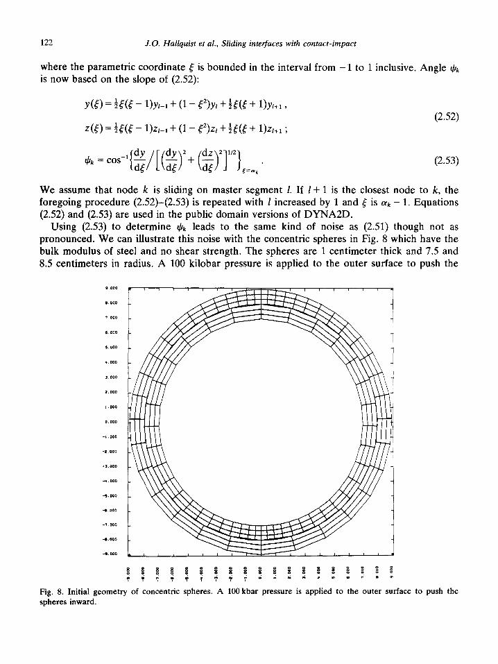
Using (2.53) to determine #k leads to the same kind of noise as (2.51) though not as pronounced. We can illustrate this noise with the concentric spheres in Fig. 8 which have the bulk modulus of steel and no shear strength. The spheres are 1 centimeter thick and 7.5 and 8.5 centimeters in radius. A 100 kilobar pressure is applied to the outer surface to push the
Fig. 8. Initial geometry of concentric spheres. A 100 kbar pressure is applied to the outer surface to push the
spheres inward.
J.O. Haliquist et al., Sliding interfaces with contact-impact 123
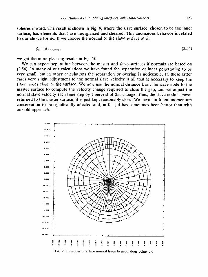
spheres inward. The result is shown in Fig. 9, where the slave surface, chosen to be the inner surface, has elements that have hourglassed and sheared. This anomalous behavior is reiated to our choice for &. If we choose the normal to the slave surface at k,
$k = ok-l,k+l, (2.54)
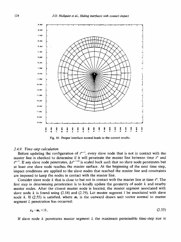
we get the more pleasing results in Fig. 10. We can expect separation between the master and slave surfaces if normals are based on
(2.54). In many of our calculations we have found the separation or inner penetration to be very small, but in other calculations the separation or overlap is noticeable. In these latter cases very slight adjustment to the normal slave velocity is all that is necessary to keep the slave nodes close to the surface. We now use the normal distance from the slave node to the master surface to compute the velocity change required to close the gap, and we adjust the normal slave velocity each time step by 1 percent of this change. Thus, the slave node is never returned to the master surface; it is just kept reasonably close. We have not found momentum conservation to be significantly affected and, in fact, it has sometimes been better than with our old approach.
124 J.O. ~a~~~~ist et at., Sliding i~te~aces with contact-impact
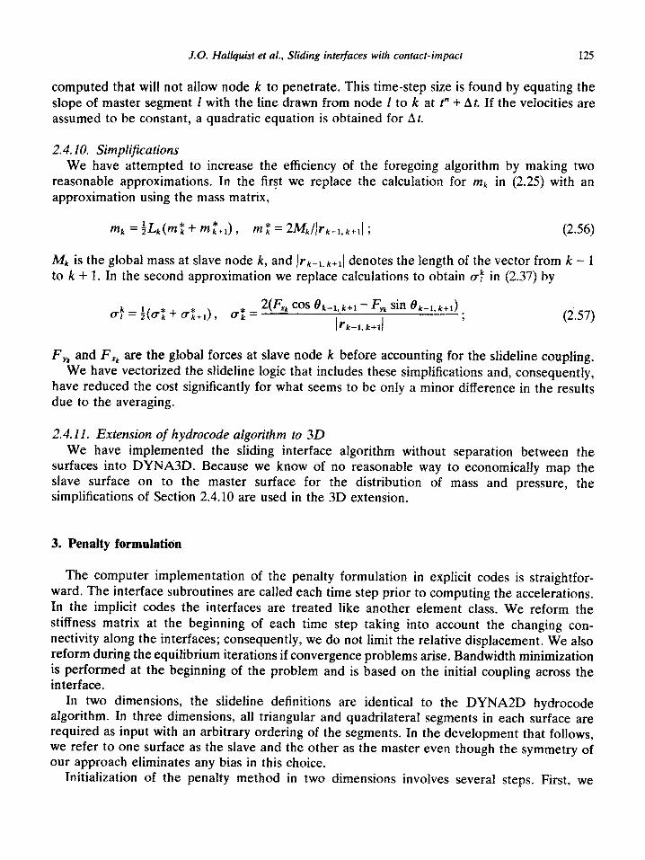
Fig. 10. Proper interface normal leads to the correct results.
2.4.9. Time-step calculation Before updating the configuration of P+‘, every slave node that is not in contact with the
master line is checked to determine if it will penetrate the master line between time t” and t “+I. If any slave node penetrates, At”+“* is scaled back such that no slave node penetrates but at least one slave node reaches the master surface. At the beginning of the next time step, impact conditions are applied to the slave nodes that reached the master line and constraints are imposed to keep the nodes in contact with the master line.
Consider slave node k that is ctose to but not in contact with the master line at time t”. The first step in determining penetration is to locally update the geometry of node k and nearby master nodes. After the closest master node is located, the master segment associated with slave node k is found using (2.18) and (2.19). Let master segment 1 be associated with slave node k. If (2.55) is satisfied, where ml is the outward drawn unit vector normal to master segment 1, penetration has occurred:
If slave node k penetrates master segment 1, the maximum permissible time-step size is
J.O. Hallquist et ai., Sliding interfaces with contact-impact 125
computed that will not allow node k to penetrate. This time-step size is found by equating the slope of master segment 1 with the line drawn from node I to k at t” + At. If the velocities are assumed to be constant, a quadratic equation is obtained for At.
2.4.10. Simplifications We have attempted to increase the efficiency of the foregoing algorithm by making two
reasonable approximations. In the first we replace the calculation for mk in (2.25) with an approximation using the mass matrix,
(2.56)
Mk is the global mass at slave node k, and Irk_l.k+l 1 denotes the length of the vector from k - 1 to k + 1. In the second approximation we replace calculations to obtain a: in (2.37) by
(2.57)
F, and F, are the global forces at slave node k before accounting for the slideline coupling, We have vectorized the slideline logic that includes these simplifications and, consequently,
have reduced the cost significantly for what seems to be only a minor difference in the results due to the averaging.
2.4.11. Extension of ~ydrocod~ aZgorit~m to 3D We have implemented the sliding interface algorithm without separation between the
surfaces into DYNA3D. Because we know of no reasonable way to economically map the slave surface on to the master surface for the distribution of mass and pressure, the simplifications of Section 2.4.10 are used in the 3D extension.
3. Penalty formulation
The computer implementation of the penalty formulation in explicit codes is straightfor- ward. The interface subroutines are called each time step prior to computing the accelerations. In the implicit codes the interfaces are treated like another element class. We reform the stiffness matrix at the beginning of each time step taking into account the changing con- nectivity along the interfaces; consequently, we do not limit the relative displacement. We also reform during the equilibrium iterations if convergence problems arise. Bandwidth minimization is performed at the beginning of the problem and is based on the initial coupling across the interface.
In two dimensions, the slideline definitions are identical to the DYNA2D hydrocode algorithm. In three dimensions, all triangular and quadrilateral segments in each surface are required as input with an arbitrary ordering of the segments. In the development that follows, we refer to one surface as the slave and the other as the master even though the symmetry of our approach eliminates any bias in this choice.
Initialization of the penafty method in two dimensions invoives several steps. First, we
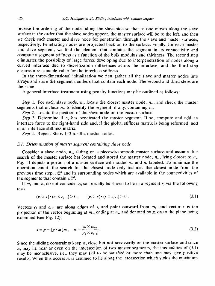
126 J.O. Hallquist et al., Sliding interfaces with contact-impact
reverse the ordering of the nodes along the slave side so that as one moves along the slave surface in the order that the slave nodes appear, the master surface will be to the left, and then we check each master and slave node for penetration through the slave and master surfaces, respectively. Penetrating nodes are projected back on to the surface. Finally, for each master and slave segment, we find the element that contains the segment in its connectivity and compute a segment stiffness as a function of the bulk modulus and thickness. The second step eliminates the possibility of large forces developing due to interpenetration of nodes along a curved interface due to discretization differences across the interface, and the third step ensures a reasonable value for the interface stiffness.
In the three-dimensional initialization we first gather all the slave and master nodes into arrays and store the segment numbers that contain each node. The second and third steps are the same.
A general interface treatment using penalty functions may be outlined as follows:
Step 1. For each slave node, IZ,, locate the closest master node, n,, and check the master segments that include n, to identify the segment, if any, containing IZ,.
Step 2. Locate the position of the slave node on the master surface. Step 3. Determine if IZ, has penetrated the master segment. If so, compute and add an
interface force to the right-hand side and, if the global stiffness matrix is being reformed, add in an interface stiffness matrix.
Step 4. Repeat Steps l-3 for the master nodes.
3.1. Determination of master segment containing slave node
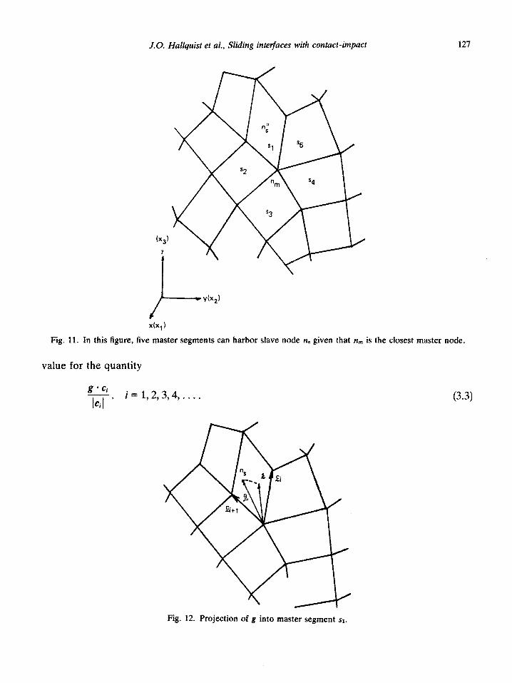
Consider a slave node, n,, sliding on a piecewise smooth master surface and assume that search of the master surface has located and stored the master node, n,, lying closest to n,. Fig. 11 depicts a portion of a master surface with nodes n, and n, labeled. To minimize the operation count, the search for the closest node only includes the closest node from the previous time step, nZd and its surrounding nodes which are available in the connectivities of the segments that contain nid.
If m, and n, do not coincide, n, can usually be shown to lie in a segment si via the following tests:
(CixS)‘(CixCi+l)>O, (Ci x S) ’ (S X Cj+l) > 0 * (3.1)
Vectors ci and ci+l are along edges of Si and point outward from m,, and vector s is the projection of the vector beginning at m,, ending at n,, and denoted by g, on to the plane being examined (see Fig. 12):
s=g-(g*mh Ci x Ci+l
m=,c,xc, ,,’ I I+
(3.2)
Since the sliding constraints keep n, close but not necessarily on the master surface and since n, may lie near or even on the intersection of two master segments, the inequalities of (3.1) may be inconclusive, i.e., they may fail to be satisfied or more than one may give positive results. When this occurs n, is assumed to lie along the intersection which yields the maximum
J.O. Ha&uist et al., Sliding interfaces with contact-impact 127
Fig. 11. In this figure, five master segments can harbor slave node II. given that n, is the closest master
value for the quantity
g l ci - 14 ’
i = 1,2,3,4,. . . . (3.3)
Fig. 12. Projection of g into master segment ~1.
128 J.O. Hallquist et al., Sliding interfaces with contact-impact
The test (3.1) is first applied to the master segment that contained the slave node in the previous step. If (3.1) is not satisfied, then each master segment that includes n,,, is checked. Our implementation does not limit the number of segments that may contain II,.
3.2. Determination of the contact point
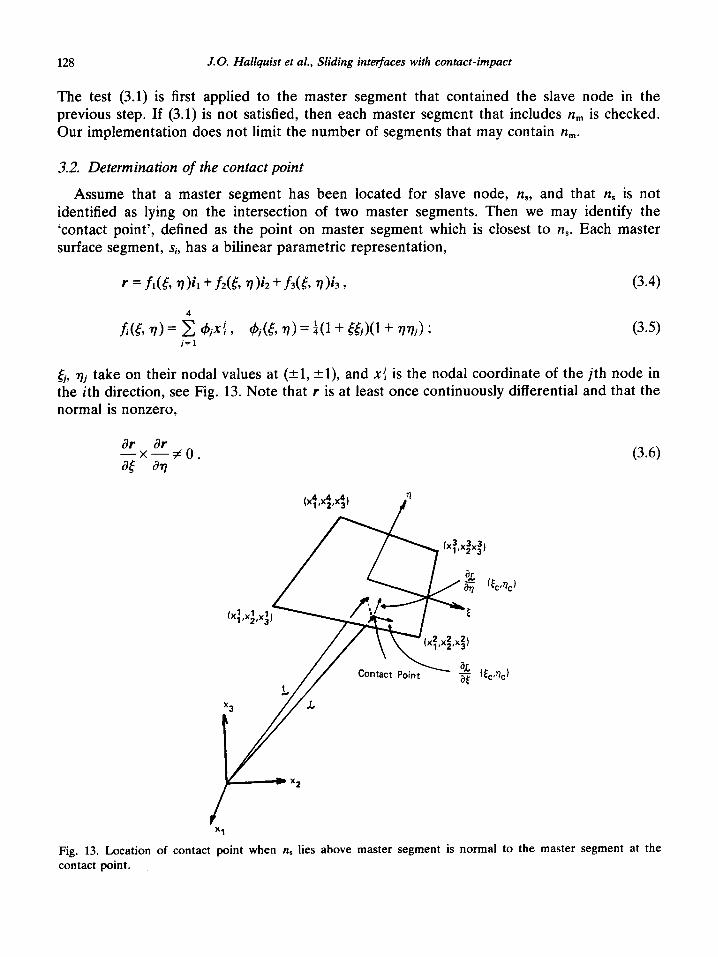
Assume that a master segment has been located for slave node, n,, and that n, is not identified as lying on the intersection of two master segments. Then we may identify the ‘contact point’, defined as the point on master segment which is closest to n,. Each master surface segment, sip has a bilinear parametric representation,
tj, r)i take on their nodal values at (kl, +l), and xj is the nodal coordinate of the jth node in the ith direction, see Fig. 13. Note that t is at least once continuously differential and that the normal is nonzero,
Fig. 13. Location of contact point when n, lies above master segment is normal to the master segment at the contact point.
J.O. Hallquist et al., Sliding interfaces with contact-impact 129
Thus, r represents a master segment that has a unique normal whose direction depends continuously on the points of si.
Let t be a position vector drawn to slave node yls and assume that the master surface segment Si has been identified with n,. The contact point coordinates (&, nC) on Si must satisfy
(3.7a)
(3.7b)
The physical problem is illustrated in Fig. 13 which shows pt, lying above the master surface. Equations (3.7a) and (3.7b) are readily solved for & in terms of rlC. One way to accomplish this is to solve (3.7a) for & in terms of no and substitute the result into (3.7b). This yields an equation in vC which is presently solved numerically in DYNA3D.
3.3. Nodal force update
Each slave node is checked for penetration through its master segment. If the slave node does not penetrate, nothing is done, but if it does, an interface force is applied between the slave node and its contact point. The magnitude of this force is proportional to the amount of penetration.
Penetration of the slave node ra,, through the master segment Si, which contains its contact point is indicated if 1 is negative,
(3.8)
If slave node n, has penetrated through master segment Si, we add an interface force vector fS that is normal to the master segment and linearly dependent on the penetration of node n,,
fS = - lkini if 1 -C 0 . (33.9)
An equal and opposite force is distributed over the master segment nodes according to
f6 = -+i(&, QJfs if 1-C 0 . (3.10)
The stiffness factor ki for master segment Si is given in terms of the bulk modulus, Kiy the volume Vi, and the face area, Ai, of the element that contains Si as
(3.11)
where fSI is a scale factor for the interface stiffness and is normally defaulted to 0.10. Larger values may cause instabilities unless the time-step size is scaled back in the time-step calculations.
130 J.O. Hallquist et al., Sliding interfaces with contact-impact
4. Examples
We present in this section five examples from diverse applications where contact-impact algorithms are necessary. None of these examples were run just for this paper; they were run on the production versions of our codes in the production-oriented engineering environment at Lawrence Livermore National Laboratory.
EXAMPLE 4.1. Muss focused projectiles. Our first example demonstrates the hydrodynamic approach to contact implemented in DYNA3D.
Mass focused projectiles, also called Misznay-Schardin munitions, are being designed as anti-armor devices. This kind of munition uses high explosives to accelerate a metal plate to a high velocity. As the plate accelerates, it is designed to deform into a cohesive shape that can penetrate thick armor. Furthermore, its shape must provide aerodynamic stability to accom- modate long standoffs from the target. Computer codes are used to iteratively develop a design with all the desired properties. Testing of the design follows to insure that everything performs as predicted.
Tuft and Godfrey [16] have computed fully three-dimensional geometries such as shown in Figs. 14 and 15 with two planes of symmetry. The time sequence of two liner cross sections is shown in Fig. 16.
Fig. 14. Basic geometry for 3D mass focused projectile device.
J.O. Hallquist et al., Sliding interfaces with contact-impact 131
Liner
5828 Nodes 4168 Elements
Fig. 15. Three-dimensional finite element mesh.
Slidelines are used between the high explosive, the liner and the case to allow the gas from the explosion to expand without restriction. The deformed shape of the liner is very sensitive to the pressure history, therefore both the detonation wave front and explosive-liner interface must be modeled carefully.
EXAMPLE 4.2. Bellows forming analysis. This example illustrates a problem involving a large amount of sliding along the contact interface. The purpose of the calculation is to determine the pressure required to collapse the stainless steel sleeve into the elastic die. Fig. 17 depicts the calculational mesh and boundary conditions.
A pressure loading is applied in 43 equal increments to a peak value of 0.580 GPa and is removed in two increments for a total of 45 steps. When the pressure reaches 0,483 GPa, the sleeve is completeIy collapsed. A sequence of deformed shapes is shown in Fig. 18 followed by the final configuration in Fig. 19.
The analysis was performed using NIKE2D; the slideline uses the penalty formulation.
EXAMPLE 4.3. Metallic O-ring. In a recent application, standard metallic O-rings were failing to produce a reliable seal. The designers felt that these failures were due to large cutouts in one of the flanges, It was felt that these cutouts, which are required for the
132 J.O. Hallquist et al., Sliding interfaces with contact-impact
t = 60 ps
t = 80 ps
t= loops
t = 14ops
Fig. 16. Time sequence of two liner cross sections.
installation gas transfer fittings, reduced the rigidity of the flange to the point where the interface pressures were insufficient for sealing.
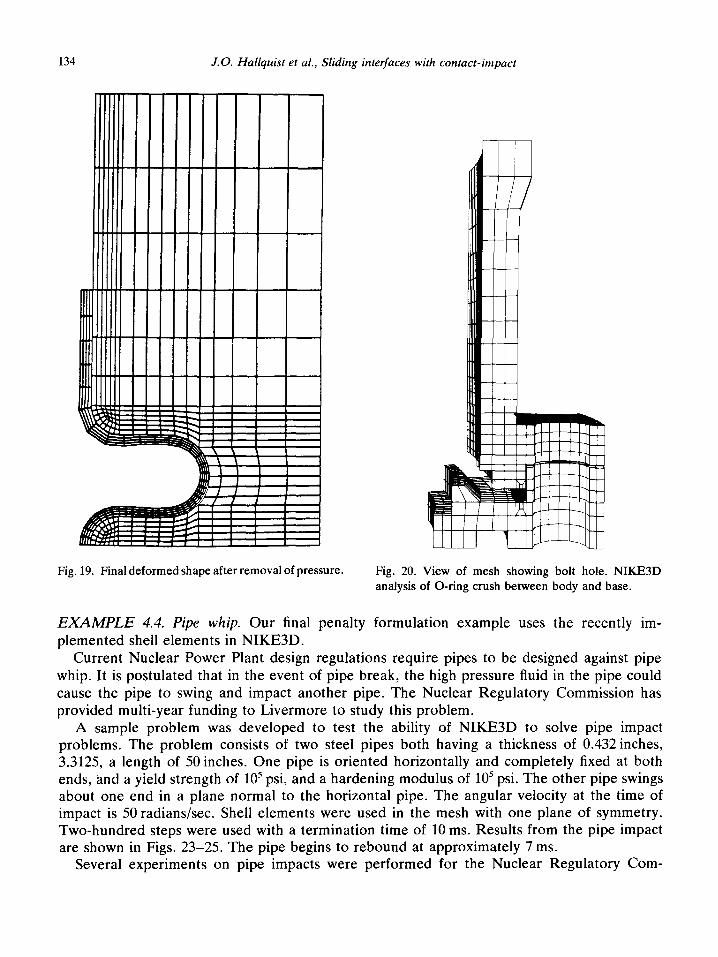
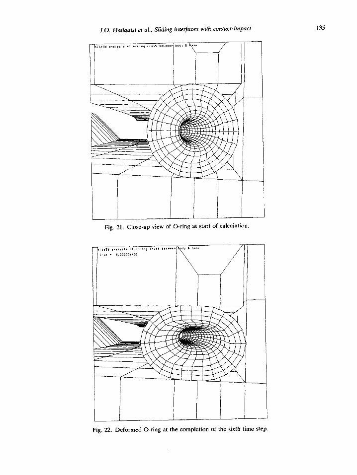
The following figures show the three-dimensional model which was used to analyze the problem. The mesh in Figs. 20 and 21 consists of 4816 nodal points and 3304 elements. Slidelines are defined between the upper portions of the O-ring and the upper flange, the lower portion of the O-ring and the lower flange, and the outer portion of the O-ring and the corresponding sealing surface of the lower flange. Additionally, a slide-surface is located between the two flanges. The model extends from the center of one of the cutouts to the center of a corresponding bolt hole. Symmetry planes are used at each of these locations to provide boundary conditions.
The total loading of the model occurs over fifteen steps. The first four steps crush the O-ring. During this portion of the loading, the O-ring undergoes large plastic strain and the interface pressures begin to develop. The next two steps are used to finish closing the gap between the two flanges. Steps eight through ten finish the bolt loading of the flanges. The upper bolt loads are sufficient to cause some plastic deformation of the upper flange. The last five steps are used to apply the gas pressure to the inside of the model. This pressurization partially unloads the O-ring. Fig. 22 shows a result of the calculation.
The NIKE3D analysis clearly showed that the cutouts were not causing the failures.
J.O. ~allquist et al., Sliding interfaces with contact-impact 133
J.O. Hallquist et al., Sliding interfaces with contact-impact
Fig. 19. Final deformed shape after removal of pressure. Fig. 20. View of mesh showing bolt hole. NIKE3D analysis of O-ring crush between body and base.
EXAMPLE 4.4. Pipe whip. Our final penalty formulation example uses the recently im- plemented shell elements in NIKE3D.
Current Nuclear Power Plant design regulations require pipes to be designed against pipe whip. It is postulated that in the event of pipe break, the high pressure fluid in the pipe could cause the pipe to swing and impact another pipe. The Nuclear Regulatory Commission has provided multi-year funding to Livermore to study this problem.
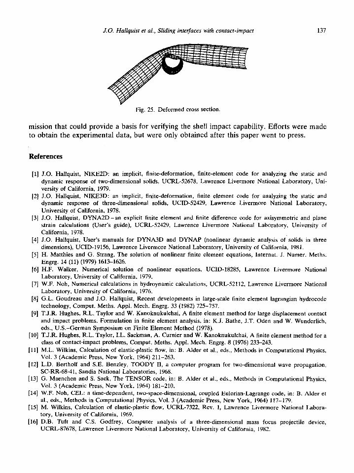
A sample problem was developed to test the ability of NIKE3D to solve pipe impact problems. The problem consists of two steel pipes both having a thickness of 0.432 inches, 3.3125, a length of 50 inches. One pipe is oriented horizontally and completely fixed at both ends, and a yield strength of lo5 psi, and a hardening modulus of 10’ psi. The other pipe swings about one end in a plane normal to the horizontal pipe. The angular velocity at the time of impact is 50 radians/set. Shell elements were used in the mesh with one plane of symmetry. Two-hundred steps were used with a termination time of 10 ms. Results from the pipe impact are shown in Figs. 23-25. The pipe begins to rebound at approximately 7 ms.
Several experiments on pipe impacts were performed for the Nuclear Regulatory Com-
J.O. ~a~i9~~st et al., Siding interfaces with contact-impact 135
Fig. 21. Close-up view of O-ring at start of calculation.
Fig. 22. Deformed O-ring at the completion of the sixth time step.
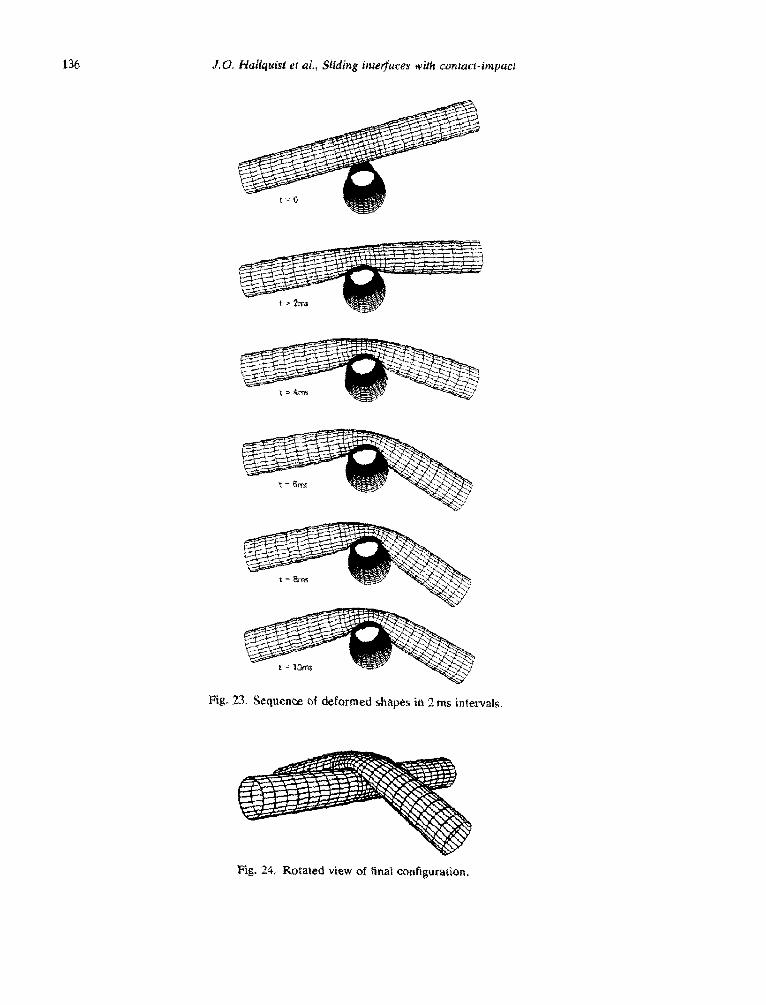
Fig. 23. Sequence of deformed shapes in 2 ms intervals.
Fig. 24. Rotated view of final configuration.
J.O. Hallquist et al., Sliding interfaces with contact-impact 137
Fig. 25. Deformed cross section.
mission that could provide a basis for verifying the shell impact capability. Efforts were made to obtain the experimental data, but were only obtained after this paper went to press.
References
111
PI
[31
[41
J.O. Hallquist, NIKE2D: an implicit, finite-deformation, finite-element code for analyzing the static and
dynamic response of two-dimensional solids, UCRL-52678, Lawrence Livermore National Laboratory, Uni-
versity of California, 1979. J.O. Hallquist, NIKE3D: an implicit, finite-deformation, finite element code for analyzing the static and dynamic response of three-dimensional solids, UCID-52429, Lawrence Livermore National Laboratory,
University of California, 1978. J.O. Hallquist, DYNA2D-an explicit finite element and finite difference code for axisymmetric and plane strain calculations (User’s guide), UCRL-52429, Lawrence Livermore National Laboratory, University of California, 1978.
J.O. Hallquist, User’s manuals for DYNA3D and DYNAP (nonlinear dynamic analysis of solids in three
dimensions), UCID-19156, Lawrence Livermore National Laboratory, University of California, 1981. [5] H. Matthies and G. Strang, The solution of nonlinear finite element equations, Internat. J. Numer. Meths.
Engrg. 14 (11) (1979) 1613-1626.
[6] H.F. Walker, Numerical solution of nonlinear equations, UCID-18285, Lawrence Livermore National Laboratory, University of California, 1979.
[7] W.F. Noh, Numerical calculations in hydroynamic calculations, UCRL-52112, Lawrence Livermore National
Laboratory, University of California, 1976. [8] G.L. Goudreau and J.O. Hallquist, Recent developments in large-scale finite element lagrangian hydrocode
technology, Comput. Meths. Appl. Mech. Engrg. 33 (1982) 725-757. [9] T.J.R. Hughes, R.L. Taylor and W. Kanoknukulchai, A finite element method for large displacement contact
and impact problems. Formulation in finite element analysis, in: K.J. Bathe, J.T. Oden and W. Wunderlich,
eds., U.S.-German Symposium on Finite Element Method (1978). [lo] T.J.R. Hughes, R.L. Taylor, I.L. Sackman, A. Curnier and W. Kanoknukulchai, A finite element method for a
[ill
w4
u31
]I41
]I51
[I61
class of contact-impact problems, Comput. Meths. Appl. Mech. Engrg. 8 (1976) 233-243.
M.L. Wilkins, Calculation of elastic-plastic flow, in: B. Alder et al., eds., Methods in Computational Physics, Vol. 3 (Academic Press, New York, 1964) 211-263. L.D. Bertholf and S.E. Benzley, TOODY II, a computer program for two-dimensional wave propagation, SC-RR-68-41, Sandia National Laboratories, 1968. G. Maenchen and S. Sack, The TENSOR code, in: B. Alder et al., eds., Methods in Computational Physics,
Vol. 3 (Academic Press, New York, 1964) 181-210. W.F. Noh, CEL: a time-dependent, two-space-dimensional, coupled Eulerian-Lagrange code, in: B. Alder et al., eds., Methods in Computational Physics, Vol. 3 (Academic Press, New York, 1964) 117-179. M. Wilkins, Calculation of elastic-plastic flow, UCRL-7322, Rev. 1, Lawrence Livermore National Labora- tory, University of California, 1969. D.B. Tuft and C.S. Godfrey, Computer analysis of a three-dimensional mass focus projectile device, UCRL-87678, Lawrence Livermore National Laboratory, University of California, 1982.