Geomorphology 204 (2014) 425–443

Contents lists available at ScienceDirect

Geomorphology

j ourna l homepage: www.e lsev ie r .com/ locate /geomorph

A numerical approach for approximating the historical morphology ofwave-dominated coasts—A case study of the Pomeranian Bight,southern Baltic Sea

Junjie Deng a, Wenyan Zhang b,c, Jan Harff a,⁎, Ralf Schneider c, Joanna Dudzinska-Nowak a, Pawel Terefenko a,Andrzej Giza a, Kazimierz Furmanczyk a

a Institute of Marine and Coastal Sciences, University of Szczecin, Mickiewicza 18, 70-383 Szczecin, Polandb MARUM—Center for Marine Environmental Sciences, University of Bremen, Leobener Str. 1, D28359 Bremen, Germanyc Institute of Physics, Ernst-Moritz-Arndt-University of Greifswald, Felix-Hausdorff-Str., 6, D17489 Greifswald, Germany

⁎ Corresponding author. Tel.: +49 381 5197 351; fax: +E-mail address: jan.harff@io-warnemuende.de (J. Harf

0169-555X/$ – see front matter © 2013 Elsevier B.V. All rhttp://dx.doi.org/10.1016/j.geomorph.2013.08.023

a b s t r a c t

a r t i c l e i n f o

Article history:Received 22 November 2012Received in revised form 13 August 2013Accepted 19 August 2013Available online 23 September 2013

A numerical approach to approximate historicalcoastal morphology is developed;The basic con-cept is a dynamic equilibrium of the coastal cross-shore profile shape;The approach can be poten-tially used for the future projection of coastlinechanges. Keywords:Coastal morphologyDynamic equilibriumSediment budget analysisCoastline configurationClimate driving forcesModeling

Comparison between historical maps from the 1900s, 1980s and amodernmap from the 2000s of the PomeranianBight at the southern Baltic Sea indicates that a major part of the coastline has been suffering continuous erosion.This also holds for a major part of other coasts on a global scale. Quantifying coastal geomorphological changeson a decadal-to-centennial temporal scale thus needs to be intensified for coastal protection activities and integrat-ed coastal zonemanagement. This study applies an estimation of sedimentmass balance including the investigationof sediment source-to-sink transport. In the case of absent historical survey data, a numerical approach, namely theDynamic Equilibrium ShoreModel (DESM), is developed to approximate the historicalmorphology and to estimatesediment budget of wave-dominated coasts based on the information of historical coastline configuration derivedfrommaps, a high-resolution modern Digital Elevation Model (DEM) and relative sea-level change. The basic con-cept of the model is a dynamic equilibrium of the coastal cross-shore profiles adapting to sediment mass balancingof a semi-enclosed coastal area, in which the unknown parameters of the cross-shore profile shapes are calculatedby numerical iterations. Themodel is applied at the Pomeranian Bight, in order to validate its capability in reflectingthe pattern of bed level change and estimating sediment mass volume. Two tests of the model are conducted inapproximating historical DEMs in 1980s and ca. 1900. The changes of approximated DEMs from past to presentare then respectively compared with the ones derived from a nautical sea chart in 1980s, and the ones producedby a complex morphodynamic model that uses the approximated DEM at ca. 1900 as a starting point to hindcastthe coastal morphological evolution of the research area. The deposition/erosion patterns along the coastline areconsistent in both comparisons. The pre-conditions and limitations of the model are discussed in detail. Themodel proposed here can serve as a useful tool for coastal morphological studies and potential applications forthe future projection of coastal morphogenesis.

© 2013 Elsevier B.V. All rights reserved.

1. Introduction

Coastal geomorphological change facilitated by a global sea-level riseand changing wind-wave climate (IPCC, 2007) is of great concern topopulations living in low-lying coastal regions. Approximation of thehistorical Digital Elevation Model (DEM) of shorelines on a decadal-to-centennial scale aims to understand the past extent of coastal morpholo-gy aswell as a derivation of sediment erosional and depositional patternsby comparison with the current coastal morphology. This provides animportant database for studying coastal morphological evolution whichserves as a reference for future coastal planning and management. Sincethe development of the Bruunmodel (Bruun, 1962, 1988), coastal profile

49 381 5197 352.f).

ights reserved.

models based on the equilibrium concepts have been used widely toanalyze coastal morphological response to sea-level change (e.g., Dean,1991; Davidson-Arnott, 2005; Wolinsky and Murray, 2009; Ashtonet al., 2011). However, extensive debate exists on whether the equilibri-um concepts are applicable to real coasts to account for non-linear re-sponses of the coastal morphology to complex physical driving forces(e.g., SCOR, 1991; Thieler et al., 2000; Cooper and Pilkey, 2004; Pilkeyand Cooper, 2004). A more accepted theory derived from these debatesis that a coastal profile is always tuning its shape to adapt to thechanges of external driving forces (e.g., winds, waves and currents)and boundary conditions (e.g., sediment input and output). In thissense the evolution of a coastal profile is a dynamic state ratherthan in a stationary equilibrium. Approximation of historical coastalmorphology thus needs to treat the coast as an integral part of thesystem to take into account the total sediment budget, rather thansplitting the system into pieces where only individual or representativeprofiles are considered.

426 J. Deng et al. / Geomorphology 204 (2014) 425–443

Hybrid (process-based formulations in combination with behavior-oriented descriptions) multi-scale, medium- to long-term (i.e., decadalup to millennial temporal scale) morphodynamic forward modelshave demonstrated their abilities in providing more insights into thefundamental driving mechanisms of non-linear complex coastal sys-tems (e.g., Cayocca, 2001; Jimenez and Arcilla, 2004; Roelvink, 2006;Wu et al., 2007; Dastgheib et al., 2008; Zhang et al., 2012), althoughtheir development is still in an early stage. Due to lack of survey data,one obstacle for the application of these complex models to a realcoast is to provide a reasonable initial status of the geomorphology.The approximation of a historical DEM is an inverse problem thatrequires a solution. Inverse modeling is a mathematical optimizationprocedure to search the best parameter of an evolutionary model origi-nally introduced by Tarantola (1987). Inversemethods have beenwide-ly applied to search the “best fit” solution in the inverse problem ofstratigraphic modeling at geological timescales characterized by hun-dreds of thousands of years (Cross and Lessenger, 1999; Bellingham,2000; Wijns et al., 2003; Charvin et al., 2009a,b, 2011). Cowell et al.

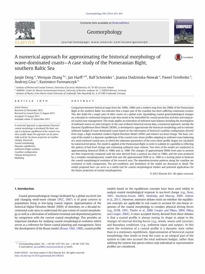
Fig. 1. Top: High-resolutionmeasured profiles in 2005 AD and corresponding best-fitted exponeThe nearshore area of the case study area (Pomeranian Bight) is divided into a series of zones

(1995) have successfully applied inverse modeling in their large-scalecoastal behavior simulation, in which profile-based coastal evolutionwas reconstructed on the Tuncurry Shelf (southeast Australia) duringand following the post-glacial marine transgression. Until the recentdecade, inverse modeling was attempted to approximate the historicalcoastal morphology at the decadal-to-centennial timescale. A pioneeringstudywas carried out by Spivack andReeve (2000)who assumed that themorphological evolution of a sea bed can be described by a linear partialdifferential equation that isolates diffusive and non-diffusive processes.The contribution of non-diffusive processes is represented by a sourceterm, which is assumed to vary slowly in the sense that changes aresmall over each time step between available data locations. The sourceterm is derived by solving an inverse problem using high-resolutionconsecutive historical bathymetric datasets of the research area.Karunarathna et al. (2008) applied this method to the Humber estuary(UK) based on historical survey data covering a period of 150 years.Based on a simplified form of the linear equation Avdeev et al. (2009)applied a similar inverse algorithm to study the annual-to-decadal

ntial functions. Note that there is an artificial dredged channel at the rivermouth; Bottom:in DESM. The offshore limit of these zones is the closure depth.

427J. Deng et al. / Geomorphology 204 (2014) 425–443

coastal profile changes at Duck (USA) and Deland (The Netherlands).These inverse models provide a reasonable approximation of the his-torical coastal morphology under the pre-condition that the sourceterm, which integrates the contribution of all non-diffusive processesto morphological change, evolves considerably slowly over the time-scale of interest. Furthermore, high-resolution survey data on a regulargrid of points at successive time steps are required to derive the sourceterm (Karunarathna et al., 2008). However, extensive historical surveydata for a coast do not always exist, especially for areas which are noteconomically important. Normally only the configuration of the historicalcoastline is available. In the case of insufficient historical survey data,a method for approximation of the historical morphology of wave-dominated coasts is proposed in this paper. The method, namelythe Dynamic Equilibrium Shore Model (DESM), uses the historical coast-line configuration, a modern high-resolution DEM, eustatic sea-levelchange and isostatic crustal movement to approximate the historicalDEM of the study area.

The paper is structured as follows. Details of themodel are describedin Section 2; model application to the Pomeranian Bight at the southernBaltic Sea, and its validation by comparison with measured historicalbathymetry and a complex long-term morphodynamic forward modelare given in Section 3. Discussion of the potential applications of themodel and its limitations is given in Section 4, with a concluding sum-mary given in Section 5.

2. The Dynamic Equilibrium Shore Model (DESM)

2.1. General modeling concept

The basic concept of DESM is that the coastal cross-shore profile shapeis assumed to evolve in a dynamic equilibrium due to its adaptation toexternal sediment sources or sinks, provided that the wind-wave climateis stable without notable change on the scale of interest (i.e., decadal-to-centennial). The study area is required to be a semi-enclosed systemwhich we defined as a coastal area with zero or only a minor net ex-change of sediment at its boundary on the temporal scale of interest. Asthe total sediment mass volume is conserved in the system, a redistribu-tion of the sediment budget (e.g. shoreline erosion and accretion) takesplace within the system induced by external driving forces (e.g., winds,waves and currents). The coastal system is divided into a series of zonesalongshore. Each zone starts from a terrestrial point which remains un-touched by hydrodynamics at the temporal scale of interest, and extendsseaward until a so-called “closure depth” (i.e., the sea bed elevation sea-ward of which remains unchanged at the temporal scale of interest). Bythis definition, each zone can be characterized by a cross-shore profileand a longshore width. Based on a high-resolution modern DEM, thehorizontal distance of coastline change is derived from a comparison be-tween the recent map and the historical map, eustatic sea-level changerecords and isostatic movement rates. Approximation of the historicalprofile shape in each zone is done in the model by iterations of themass volume redistribution within the system.

Dean's power law has been used widely to approximate the beachprofile within the breaker zone (Dean, 1991). Despite of this, the expo-nential function presented by Bodge (1992) and Komar and Mcdougal(1994) appears to bemore appropriate to approximate the concave pro-file shape of thewhole shoreface, as the limit of the exponential decay inthe function curve might be related to the limit of offshore decay ofsediment movement, in contrast to an infinite depth of the Dean'spower law function. On the other hand, exponential functions fit thehigh-resolution modern profile measurement data of the PomeranianBight ideally. The R2 value is used to test the fitness of the functions inall 153 profiles. The exponential function with an average R2 value of0.88 fits the profile better than any other widely used power law func-tion (e.g. Dean, 1991) with an average R2 value of 0.85. The 2/3-powerlaw function doesn't fit the whole shoreface profile, exhibiting an

average R2 value of only−0.40. Examples of using the best-fit functionare given in Fig. 1.

Assuming that the present bathymetric profile shape is described bythe exponential function:

y0 ¼ a0 1−eb0x� �

ð1Þ

and the historical bathymetrical profile is given by:

y1 ¼ a1 1−eb1 x−cð Þ� �−s ð2Þ

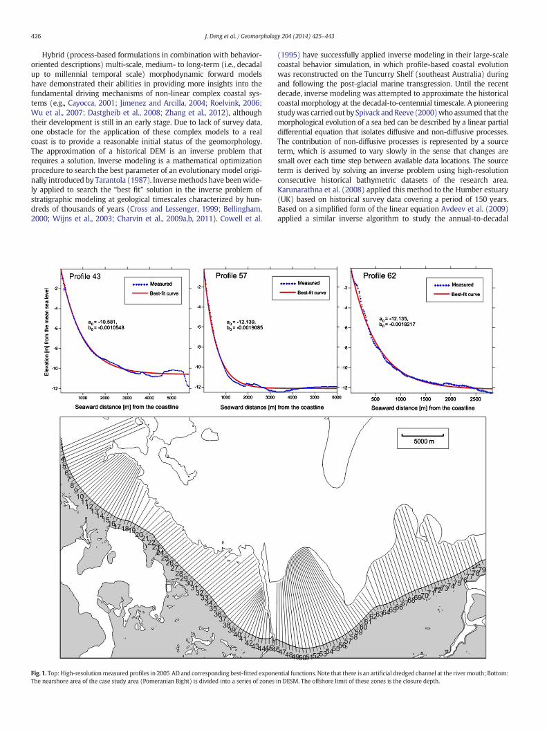
where the subscript ‘0’ refers to the coefficients of the present profileshape and subscript ‘1’ for the coefficients of the historical profile. a0and a1 are the limit of the profile where the depth of the profile tendsto be constant, b0 and b1 are the curvature coefficients of the recentand historical profiles, respectively. c is the coastline displacement forthe given time span. s is the relative sea-level change that is the sumof the eustatic sea-level change and the glacial isostatic adjustment. Asketch of the comparison between recent and historical profile shapes(in a retreating type) in the model is illustrated in Fig. 2.

The upper part of the profile is a highly dynamic environment, withprocesses such as wave breaking which causes a large amount of waveenergy to be transformed into turbulent kinetic energy, inducing a con-siderable increase in mass and momentum transport. Sediment in thelower part is stirred by wave action only during an extreme event(e.g., storm). In the model application, depending on the temporalscale of interest, the closure depth of a coastal area is derived eitherfrom a comparison between survey maps (if available) or the knowl-edge of the site. During a given time span, the value of the closuredepth remains constant, and it is assumed to increasewith an increasedtemporal scale of interest. The closure depth is assumed to be related tothe temporal scale of interest, as Nicholls et al. (1998) found that theclosure depth tends to increase with time. The increase of closuredepthmight be related to a long-term accumulation effect of small mor-phological change in a short time span. The residual sediment move-ment is considered as a dominant factor for morphological changeover a long time and large spatial scale in a quantitative simulation oflarge-scale coastal behavior by Cowell et al. (1995). Thus the historicalcoefficient a1 of the offshore limit of exponential function is assumedto be equal to the present one, which yields:

a1 ¼ a0 ð3Þ

By the meaning of Eq. (3), the lower part of the historical profile(Fig. 2) might be accommodated after the relative sea-level change.Note that the offshore limit of the exponential function might not beequal to the closure depth, which depends on the profile curvature andwhether the limit of the profile is already the closure depth for a giventime span.

In the model, the sources and sinks of sediment from the longshoreand cross-shore directions are taken into account as one gross sedimentbudget, marked as Vexternal. Fig. 2 illustrates the mass volume of erosionand deposition in the two dimensional cross-shore profile system. Thisgives the equation below:

Verosion−Vdeposition ¼ Vexternal ð4Þ

where Verosion represents the eroded mass volume in the upper part ofthe historical profile and Vdeposition represents the deposited mass vol-ume in the lower part of the historical profile. The transition pointfrom erosion to deposition is marked as x0 representing the seawarddistance from presentwaterline (the term ‘waterline’ in this context re-fers to the line where the sea meets the land at its mean level).

Fig. 2. Sketch of the recent and historical profile shapes (retreating type) in DESM.

428 J. Deng et al. / Geomorphology 204 (2014) 425–443

The value of x0 is obtained by:

a1 1−eb1 x0−cð Þ� �−s ¼ a0 1−eb0x0

� �ð5Þ

where c is the retreated distance (m) and s is relative sea-level rise (m).There are two unknown parameters in Eq. (5): x0 and b1. If b1 = b0, x0can be solved analytically as given below:

x0 ¼ 1b0

lns

a0 1−e−b0c� � ð6Þ

Otherwise it has to be solved iteratively together with b1 by aninverse procedure, which will be described in Section (2.4). Verosionand Vdeposition are calculated by an integration of the exponential func-tion, which are given by Eqs. (7) and (8), respectively.

Verosion ¼Z x0

ca1 1−eb1 x−cð Þ� �

−s−a0 1−eb0x� �

0� �

dx

þZ c

0

−sc

x−a0 1−eb0x� �

0dx� �

ð7Þ

Vdeposition ¼Z x�

x0

a0 1−eb0x� �

0−a1 1−eb1 x−cð Þ� �1 þ s

� �dx ð8Þ

Vexternal is critical in determining the historical profile shape. In thisinverse task, the remaining unknown coefficient is b1 which changesthe internal volume of the profile. For retreating coasts, Verosion de-creases and Vdeposition increases along with a decreasing value of b1,thus Vexternal decreases, vice versa. The procedure is opposite for aprograding coast.

Normally, the external volume Vexternal for a single profile is ratherdifficult to estimate due to an influence of longshore sediment trans-port. Longshore sediment transport flux at a wave-dominated coastmay be reasonably estimated on a seasonal-to-annual scale based onconsecutive profile measurement data (Zhang et al., 2013), however itwould be a difficult task on a decadal-to-centennial scale. This is notonly due to a lack of profile measurement data covering such a longtime span, but also due to the oscillations of wind-wave climate,which introduces high complexity into the morphodynamic system.One possible way to overcome this problem is to analyze the redistribu-tion of sediment budget in a semi-enclosed coastal system, inwhich thetotal sedimentmass is conserved. Thismeans the sediment eroded from

one individual profile partly deposits on the lower part of the profile andpartly transports by longshore currents to other profileswhich arewith-in the system. One similar example is given by Schwarzer et al. (2003)who studied the coastline change of the Pomeranian Bight on a centen-nial scale based on an estimation of total sediment budget. In a semi-enclosed coastal system, there are both accumulation and erosionparts, which define two coastal types. Owing to the opposite processof erosion and accumulation, morphological evolutions of these twocoastal types have different behaviors. Moreover, Cowell et al. (1995)and Wolinsky and Murray (2009) found that the cliff coast and barrierisland coast behave differently when they retreat. Thus, the cliff partand the dune part of the study area are calculated separately in themodel.

2.2. Calculation of coastal retreat

In a semi-enclosed coastal system, the net sediment budget in bothalong-shore and cross-shore directions is zero. However, non-zero netsediment budget could exist for each zone within the system.

The whole coastal retreating part of the study area is divided into n1zones with a uniform width Δh, each is represented by a cross-shoreprofile. The total volume change of the retreating coastal section isthus given by:

ΔhXn1

i¼1

Verosion;i−Vdeposition;i

� �¼Δh

Xn1i¼1

Vexternal;i ð9Þ

The sum of Vexternal,ion the right hand side indicates the total massvolume lost from the retreated coastal zones, which provides the sourcefor prograding zones in the system.

2.2.1. Cliff coastFor a retreat of the cliff coast (as shown in Fig. 3, top), a uniform re-

sponse rate of the submarine profile curvature is assumed in DESM forall cliff-backed zones:

b1b0

¼ const ð10Þ

A stationary equilibrium profile shape (i.e., the Bruun model) isreached when const = 1. If const does not equal 1, it means there is a

429J. Deng et al. / Geomorphology 204 (2014) 425–443

non-zero net sediment transport at the boundary of the zone. An in-verse procedure (which will be described in Section 2.4) is then usedto calculate const. The subaerial profile of the retreated cliff is assumedto be equal to the present one.

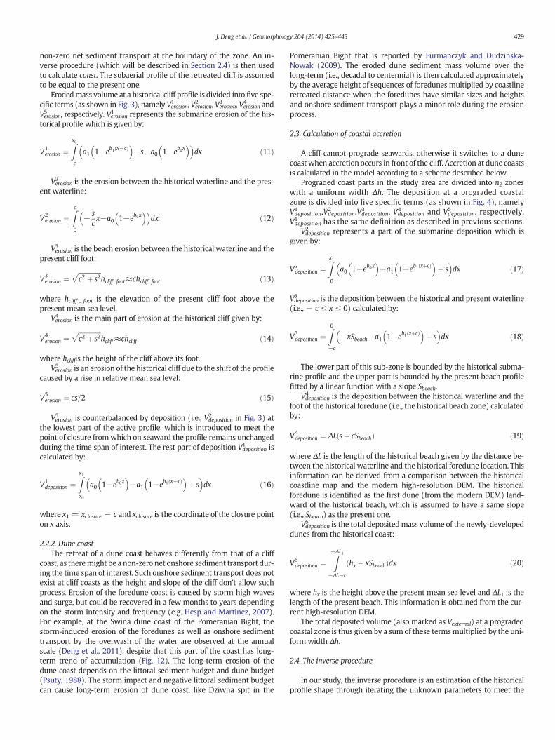
Erodedmass volume at a historical cliff profile is divided into five spe-cific terms (as shown in Fig. 3), namely Verosion

1 , Verosion2 , Verosion3 , Verosion4 andVerosion5 , respectively. Verosion1 represents the submarine erosion of the his-

torical profile which is given by:

V1erosion ¼

Zx0

c

a1 1−eb1 x−cð Þ� �−s−a0 1−eb0x

� �� �dx ð11Þ

Verosion2 is the erosion between the historical waterline and the pres-

ent waterline:

V2erosion ¼

Zc

0

− scx−a0 1−eb0x

� �� �dx ð12Þ

Verosion3 is the beach erosion between the historical waterline and the

present cliff foot:

V3erosion ¼

ffiffiffiffiffiffiffiffiffiffiffiffiffiffiffic2 þ s2

phcliff foot≈chcliff foot ð13Þ

where hcliff _ foot is the elevation of the present cliff foot above thepresent mean sea level.

Verosion4 is the main part of erosion at the historical cliff given by:

V4erosion ¼

ffiffiffiffiffiffiffiffiffiffiffiffiffiffiffic2 þ s2

phcliff≈chcliff ð14Þ

where hcliffis the height of the cliff above its foot.Verosion5 is an erosion of the historical cliff due to the shift of the profile

caused by a rise in relative mean sea level:

V5erosion ¼ cs=2 ð15Þ

Verosion5 is counterbalanced by deposition (i.e., Vdeposition2 in Fig. 3) at

the lowest part of the active profile, which is introduced to meet thepoint of closure fromwhich on seaward the profile remains unchangedduring the time span of interest. The rest part of deposition Vdeposition

1 iscalculated by:

V1deposition ¼

Zx1

x0

a0 1−eb0x� �

−a1 1−eb1 x−cð Þ� �þ s

� �dx ð16Þ

where x1 = xclosure − c and xclosure is the coordinate of the closure pointon x axis.

2.2.2. Dune coastThe retreat of a dune coast behaves differently from that of a cliff

coast, as theremight be a non-zero net onshore sediment transport dur-ing the time span of interest. Such onshore sediment transport does notexist at cliff coasts as the height and slope of the cliff don't allow suchprocess. Erosion of the foredune coast is caused by storm high wavesand surge, but could be recovered in a few months to years dependingon the storm intensity and frequency (e.g. Hesp and Martinez, 2007).For example, at the Swina dune coast of the Pomeranian Bight, thestorm-induced erosion of the foredunes as well as onshore sedimenttransport by the overwash of the water are observed at the annualscale (Deng et al., 2011), despite that this part of the coast has long-term trend of accumulation (Fig. 12). The long-term erosion of thedune coast depends on the littoral sediment budget and dune budget(Psuty, 1988). The storm impact and negative littoral sediment budgetcan cause long-term erosion of dune coast, like Dziwna spit in the

Pomeranian Bight that is reported by Furmanczyk and Dudzinska-Nowak (2009). The eroded dune sediment mass volume over thelong-term (i.e., decadal to centennial) is then calculated approximatelyby the average height of sequences of foredunes multiplied by coastlineretreated distance when the foredunes have similar sizes and heightsand onshore sediment transport plays a minor role during the erosionprocess.

2.3. Calculation of coastal accretion

A cliff cannot prograde seawards, otherwise it switches to a dunecoast when accretion occurs in front of the cliff. Accretion at dune coastsis calculated in the model according to a scheme described below.

Prograded coast parts in the study area are divided into n2 zoneswith a uniform width Δh. The deposition at a prograded coastalzone is divided into five specific terms (as shown in Fig. 4), namelyVdeposition1 ,Vdeposition

2 ,Vdeposition3 , Vdeposition

4 and Vdeposition5 , respectively.

Vdeposition1 has the same definition as described in previous sections.Vdeposition2 represents a part of the submarine deposition which is

given by:

V2deposition ¼

Zx1

0

a0 1−eb0x� �

−a1 1−eb1 xþcð Þ� �þ s

� �dx ð17Þ

Vdeposition3 is the deposition between the historical and present waterline

(i.e., − c ≤ x ≤ 0) calculated by:

V3deposition ¼

Z0

−c

−xSbeach−a1 1−eb1 xþcð Þ� �þ s

� �dx ð18Þ

The lower part of this sub-zone is bounded by the historical subma-rine profile and the upper part is bounded by the present beach profilefitted by a linear function with a slope Sbeach.

Vdeposition4 is the deposition between the historical waterline and the

foot of the historical foredune (i.e., the historical beach zone) calculatedby:

V4deposition ¼ ΔL sþ cSbeachð Þ ð19Þ

where ΔL is the length of the historical beach given by the distance be-tween the historical waterline and the historical foredune location. Thisinformation can be derived from a comparison between the historicalcoastline map and the modern high-resolution DEM. The historicalforedune is identified as the first dune (from the modern DEM) land-ward of the historical beach, which is assumed to have a same slope(i.e., Sbeach) as the present one.

Vdeposition5 is the total depositedmass volume of the newly-developed

dunes from the historical coast:

V5deposition ¼

Z−ΔL1

−ΔL−c

hx þ xSbeachð Þdx ð20Þ

where hx is the height above the present mean sea level and ΔL1 is thelength of the present beach. This information is obtained from the cur-rent high-resolution DEM.

The total deposited volume (also marked as Vexternal) at a progradedcoastal zone is thus given by a sumof these termsmultiplied by the uni-form width Δh.

2.4. The inverse procedure

In our study, the inverse procedure is an estimation of the historicalprofile shape through iterating the unknown parameters to meet the

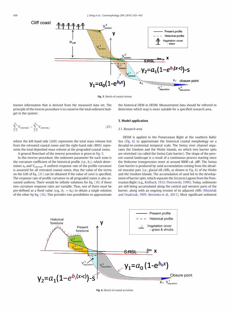
Fig. 3. Sketch of coastal retreat.

430 J. Deng et al. / Geomorphology 204 (2014) 425–443

known information that is derived from the measured data set. Theprinciple of the inverse procedure is to conserve the total sediment bud-get in the system:

Xn1i¼1

Vexternal;i ¼Xn2j¼1

Vexternal; j ð21Þ

where the left-hand side (LHS) represents the total mass volume lostfrom the retreated coastal zones and the right-hand side (RHS) repre-sents the total deposited mass volume at the prograded coastal zones.

A general flowchart of the inverse procedure is given in Fig. 5.In this inverse procedure, the unknown parameter for each zone is

the curvature coefficient of the historical profile (i.e., b1), which deter-mines x0 and Vexternal. A uniform response rate of the profile curvatureis assumed for all retreated coastal zones, thus the value of the termson the LHS of Eq. (21) can be obtained if the value of const is specified.The response rate of profile curvature in all prograded zones is also as-sumed uniform. There would be infinite solutions for Eq. (16) if thesetwo curvature response rates are variable. Thus, one of them must bepre-defined as a fixed value (e.g., b1 = b0) to obtain a single solutionof the other by Eq. (16). This provides two possibilities to approximate

Fig. 4. Sketch of coa

the historical DEM in DESM. Measurement data should be referred todetermine which way is more suitable for a specified research area.

3. Model application

3.1. Research area

DESM is applied to the Pomeranian Bight at the southern BalticSea (Fig. 6) to approximate the historical coastal morphology on adecadal-to-centennial temporal scale. The Swina river channel sepa-rates the Usedom and the Wolin Islands, on which two barrier spitsare stretched (so called the Swina Gate barrier). The shape of the pres-ent coastal landscape is a result of a continuous process starting sincethe Holocene transgression onset at around 8000 cal. aBP. The SwinaGate barrier is produced by sand accumulation coming from the abrad-ed moraine part (i.e., glacial till cliffs, as shown in Fig. 6) of the Wolinand the Usedom Islands. The accumulation of sand led to the develop-ment of barrier spits, which separate the Szczecin Lagoon from thePom-eranian Bight (e.g., Keilhack, 1912; Piotrowski, 1999). Today, sedimentsare still being accumulated along the central and western parts of thebarrier, along with an ongoing erosion of its adjacent cliffs (Musielakand Osadczuk, 1995; Borowka et al., 2011). Most significant sediment

stal accretion.

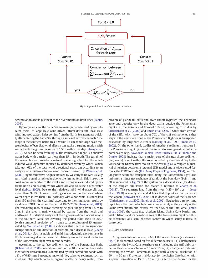
Fig. 5. A general flowchart of the inverse procedure.

431J. Deng et al. / Geomorphology 204 (2014) 425–443

accumulation occurs just next to the river mouth on both sides (Labuz,2005).

Hydrodynamics of theBaltic Sea aremainly characterized by compli-cated meso- to large-scale wind-driven littoral drifts and local-scalewind-inducedwaves. Tides coming from theNorth Sea attenuate quick-ly after entering the Baltic Sea through a series of narrow channels. Tiderange in the southern Baltic area is within 15 cm, while large-scale me-teorological effects (i.e. wind effects) can excite a surging motion withwater level changes in the order of 1.5 m within one day (Zhang et al.,2010). As can be seen from Fig. 6, the Pomeranian Bight is a shallowwater body with a major part less than 15 m in depth. The terrain ofthe research area provides a natural sheltering effect for the wind-induced wave dynamics induced by dominant westerly winds, whichtake up ~65% of the total wind directional spectrum according to ananalysis of a high-resolution wind dataset derived by Weisse et al.(2009). Significant wave heights induced by westerly winds are usuallyrestricted to small amplitudes due to the limited fetch. This makes thecoast more vulnerable to the swells and strong waves induced by ex-treme north and easterly winds which are able to cause a high waterlevel (Labuz, 2005). Due to the relatively mild wind-wave climate,more than 99.8% of wave breakings occur within the area wherewater depth is less than 2 m (normally with a horizontal distance lessthan 150 m from the coastline) according to the simulation results bya validated 2DH model for the period 1997–2006 (Zhang et al., 2013).The remaining 0.2% of wave breaking heights, ranging from 1.5 m to2 m, in this area is mainly caused by storms from the north andnorth–east. A statistical analysis of the high-resolution hindcast windsat the southern Baltic Sea covering the period from 1948 to 2007(with a temporal resolution of 1 h and spatial resolution of 25 km pro-vided by Weisse et al. (2009)) indicates that there is no significantchange either on the direction or strength on a decadal scale (Zhanget al., 2011a). Such a stable and mild hydrodynamic environment inthe time-averaged sense caused a relatively smooth coastal evolutionof the Pomeranian Bight over recent decades.

According to the surface sediment map of the Pomeranian Bight(Bobertz et al., 2006), nearshore (within the 10 m contour line) sedi-ment of the research area is dominated by well-sorted fine sands witha D50 of 0.25 mm. Suspended material (i.e., cohesive sediment such asmud and clay which contains organic matter or heavy metal) from

erosion of glacial till cliffs and river runoff bypasses the nearshorezone and deposits only in the deep basins outside the PomeranianBight (i.e., the Arkona and Bornholm Basin) according to studies byChristiansen et al. (2002) and Emeis et al. (2002). Sands from erosionof the cliffs, which take up about 70% of the cliff components, eitherstays in the nearshore zone of the Pomeranian Bight or is transportedeastwards by longshore currents (Diesing et al., 1999; Emeis et al.,2002). On the other hand, studies of longshore sediment transport inthe Pomeranian Bight by several researchers focussing on different tem-poral scales (e.g., Zawadzka-Kahlau, 1999; Pruszak, 2003; Froehle andDimke, 2008) indicate that a major part of the nearshore sediment(i.e., sands) is kept within the zone bounded by Greifswald Bay to thewest and the Dziwna river mouth to the east (Fig. 6). A coupled numer-ical simulation between a regional 2DH model and a widely-used for-mula, the CERC formula (U.S. Army Corps of Engineers, 1984), for totallongshore sediment transport rates along the Pomeranian Bight alsoindicates a minor net exchange of sands at the boundary (Point 1 and50 as indicated in Fig. 7) of the system on a decadal scale (for detailsof the coupled simulation the reader is referred to Zhang et al.(2013)). The sediment load from the river (425 ∗ 103 t yr−1; Leipeet al., 1998) is mainly suspended fines that deposit as mud either inthe lagoon (Borówka et al., 2005) or in deeper basins of the Baltic Sea(Christiansen et al., 2002; Emeis et al., 2002). Neglecting a minor sandinput from the river, which deposits immediately in the vicinity of theSwina river mouth and covers less than 5% of the total area (Emeiset al., 2002), the coast (i.e., Usedom Island, Swina Gate barrier andWolin Island) and its nearshore area of the Pomeranian Bight can thusbe considered as a semi-enclosed system in which sandy material isconserved.

3.2. Data description

A high-resolution modern DEM of the research area (as shown inFig. 6) is elaborated based on five different datasets: (1) a bathymetricdataset for the Swina Gate nearshore area (including the artificial chan-nel)with a spatial resolution of 15 m × 15 m; (2) a bathymetric datasetcovering the whole Pomeranian Bight with a spatial resolution of50 m × 50 m; (3) a terrestrial dataset for the Swina Gate barrier witha spatial resolution of 15 m × 15 m; (4) a terrestrial dataset for the

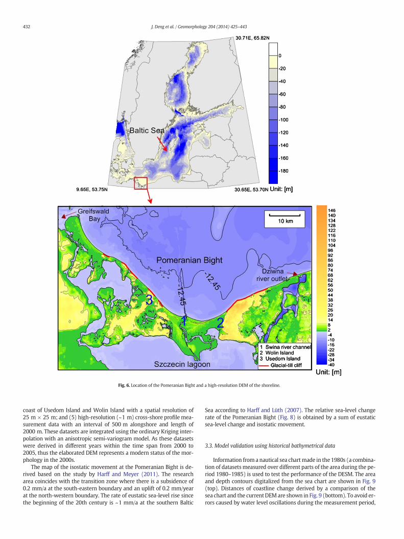
Fig. 6. Location of the Pomeranian Bight and a high-resolution DEM of the shoreline.

432 J. Deng et al. / Geomorphology 204 (2014) 425–443

coast of Usedom Island and Wolin Island with a spatial resolution of25 m × 25 m; and (5) high-resolution (~1 m) cross-shore profile mea-surement data with an interval of 500 m alongshore and length of2000 m. These datasets are integrated using the ordinary Kriging inter-polation with an anisotropic semi-variogram model. As these datasetswere derived in different years within the time span from 2000 to2005, thus the elaborated DEM represents a modern status of the mor-phology in the 2000s.

The map of the isostatic movement at the Pomeranian Bight is de-rived based on the study by Harff and Meyer (2011). The researcharea coincides with the transition zone where there is a subsidence of0.2 mm/a at the south-eastern boundary and an uplift of 0.2 mm/yearat the north-western boundary. The rate of eustatic sea-level rise sincethe beginning of the 20th century is ~1 mm/a at the southern Baltic

Sea according to Harff and Lüth (2007). The relative sea-level changerate of the Pomeranian Bight (Fig. 8) is obtained by a sum of eustaticsea-level change and isostatic movement.

3.3. Model validation using historical bathymetrical data

Information from a nautical sea chartmade in the 1980s (a combina-tion of datasetsmeasured over different parts of the area during the pe-riod 1980–1985) is used to test the performance of the DESM. The areaand depth contours digitalized from the sea chart are shown in Fig. 9(top). Distances of coastline change derived by a comparison of thesea chart and the currentDEMare shown in Fig. 9 (bottom). To avoid er-rors caused by water level oscillations during the measurement period,

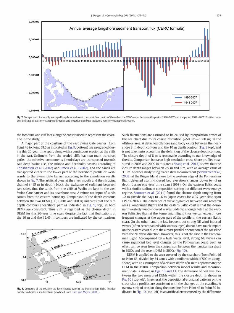
Fig. 7. Comparison of annually averaged longshore sediment transport flux (unit: m3) based on the CERCmodel between the period 1980–2007 and the period 1948–2007. Positive num-bers indicate an easterly transport direction and negative numbers indicate a westerly transport direction.

433J. Deng et al. / Geomorphology 204 (2014) 425–443

the foredune and cliff foot along the coast is used to represent the coast-line in the study.

A major part of the coastline of the east Swina Gate barrier (fromPoint 46 to Point 58.5 as indicated in Fig. 9, bottom) has prograded dur-ing this 20-year time span, along with a continuous erosion at the cliffsin the east. Sediment from the eroded cliffs has two main transportpaths: the cohesive components (mud/clay) are transported towardstwo deep basins (i.e., the Arkona and Bornholm basins) according toChristiansen et al. (2002) and Emeis et al. (2002), and the sands aretransported either to the lower part of the nearshore profile or west-wards to the Swina Gate barrier according to the simulation resultsshown in Fig. 7. The artificial piers at the river mouth and the shippingchannel (~15 m in depth) block the exchange of sediment betweentwo sides, thus the sands from the cliffs at Wolin are kept to the eastSwina Gate barrier and its nearshore area. A minor net input of sandscomes from the eastern boundary. Comparison of the depth contoursbetween the two DEMs (i.e., 1980s and 2000s) indicates that the 8 mdepth contours (nearshore part as indicated in Fig. 9, top) in bothDEMs are consistent. Thus 8 m is regarded as the closure depth inDESM for this 20-year time span, despite the fact that fluctuations atthe 10 m and the 12.45 m contours are indicated by the comparison.

Fig. 8. Contours of the relative sea-level change rate in the Pomeranian Bight. Positivenumber indicates a sea-level rise (modified from Harff and Meyer (2011)).

Such fluctuations are assumed to be caused by interpolation errors ofthe sea chart due to its coarse resolution (~500 m–~1000 m) in theoffshore area. A detached offshore sand body exists between the near-shore 8 m depth contour and the 10 m depth contour (Fig. 9 top), andis not taken into account in the definition of the closure depth contour.The closure depth of 8 m is reasonable according to our knowledge ofthe site. Comparison between high-resolution cross-shore profilesmea-sured in 2005 and 2009 in this area (Zhang et al., 2013) shows that theclosure depth ranges between 2.5 m and 6 m, with an average value of3.5 m. Another study using tracer stick measurement (Schwarzer et al.,2003) at the Rügen Island close to the western edge of the PomeranianBight detected storm-induced bed elevation changes down to ~5 mdepth during one year time span (1998). On the eastern Baltic coastwith a similar sediment composition setting but different wave energyregime, Soomere et al. (2011) found the closure depth ranging from~2 m (inside the bay) to ~6 m (open coast) for a 37-year time span(1970–2007). The difference of wave dynamics between our researcharea (Pomeranian Bight) and the eastern Baltic coast is that the domi-nant westerly wind-induced waves undergo a longer fetch at the east-ern Baltic Sea than at the Pomeranian Bight, thus we can expect morefrequent changes at the upper part of the profile in the eastern Balticcoast. On the other hand the less frequent but strong NE wind-inducedwaves (often accompanied with storm surges) do not have much impacton the eastern coast due to the almost parallel orientation of the coastlinewith the NE wave direction. However, this is not the case in the Pomera-nian Bight. Accompanied by a high water level, strong NE waves cancause significant bed level changes on the Pomeranian coast. Such aneffect can be seen from the comparison between the nautical sea chartin 1980s and the recent DEM in 2000s (Fig. 10).

DESM is applied to the area covered by the sea chart (from Point 46to Point 63, divided by 34 zones with a uniform width of 500 m along-shore)with an assumption of a closure depth of 8 m to approximate theDEM in the 1980s. Comparison between model results and measure-ment data is shown in Figs. 10 and 11. The difference of bed level be-tween the two measured DEMs within the closure depth is shown inFig. 10 (top-left). In general, the depositional/erosional patterns on thecross-shore profiles are consistent with the changes at the coastline. Anarrow strip of erosion along the coastline from Point 46 to Point 59 in-dicated in Fig. 10 (top-left) is an artificial error caused by the difference

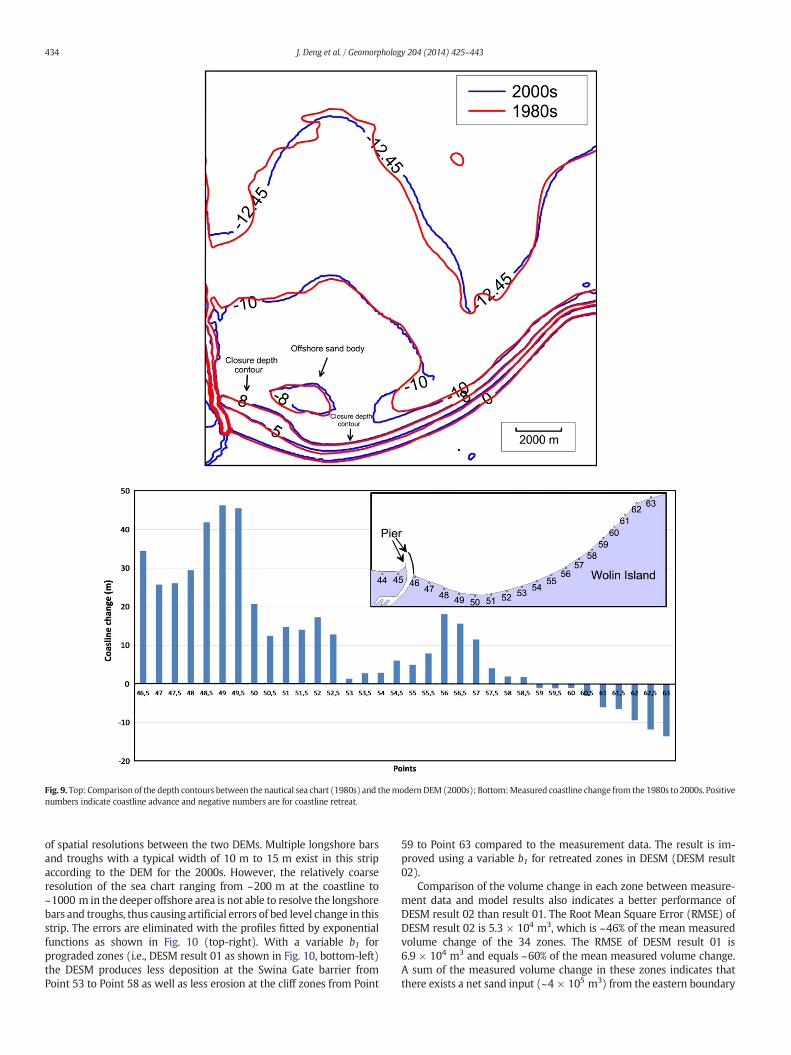
Fig. 9. Top: Comparison of the depth contours between the nautical sea chart (1980s) and themodernDEM (2000s); Bottom:Measured coastline change from the 1980s to 2000s. Positivenumbers indicate coastline advance and negative numbers are for coastline retreat.

434 J. Deng et al. / Geomorphology 204 (2014) 425–443

of spatial resolutions between the two DEMs. Multiple longshore barsand troughs with a typical width of 10 m to 15 m exist in this stripaccording to the DEM for the 2000s. However, the relatively coarseresolution of the sea chart ranging from ~200 m at the coastline to~1000 m in the deeper offshore area is not able to resolve the longshorebars and troughs, thus causing artificial errors of bed level change in thisstrip. The errors are eliminated with the profiles fitted by exponentialfunctions as shown in Fig. 10 (top-right). With a variable b1 forprograded zones (i.e., DESM result 01 as shown in Fig. 10, bottom-left)the DESM produces less deposition at the Swina Gate barrier fromPoint 53 to Point 58 as well as less erosion at the cliff zones from Point

59 to Point 63 compared to the measurement data. The result is im-proved using a variable b1 for retreated zones in DESM (DESM result02).

Comparison of the volume change in each zone between measure-ment data and model results also indicates a better performance ofDESM result 02 than result 01. The Root Mean Square Error (RMSE) ofDESM result 02 is 5.3 × 104 m3, which is ~46% of the mean measuredvolume change of the 34 zones. The RMSE of DESM result 01 is6.9 × 104 m3 and equals ~60% of the mean measured volume change.A sum of the measured volume change in these zones indicates thatthere exists a net sand input (~4 × 105 m3) from the eastern boundary

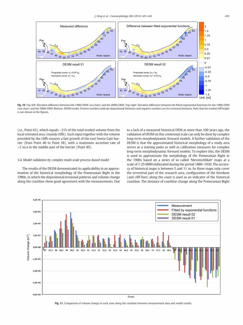
Fig. 10. Top-left: Elevation difference between the 1980s DEM (sea chart) and the 2000s DEM; Top-right: Elevation difference between the fitted exponential functions for the 1980s DEM(sea chart) and the 2000s DEM; Bottom:DESM results. Positive numbers indicate depositional thickness and negative numbers are for erosional thickness. Note that the eroded cliff heightis not shown in the figures.

435J. Deng et al. / Geomorphology 204 (2014) 425–443

(i.e., Point 63), which equals ~21% of the total eroded volume from thelocal retreated area (mainly cliffs). Such input togetherwith the volumeprovided by the cliffs ensures a fast growth of the east Swina Gate bar-rier (from Point 46 to Point 58), with a maximum accretion rate of~2 m/a in the middle part of the barrier (Point 49).

3.4. Model validation by complex multi-scale process-based model

The results of the DESMdemonstrated its applicability in an approx-imation of the historical morphology of the Pomeranian Bight in the1980s, in which the depositional/erosional patterns and volume changealong the coastline show good agreement with the measurements. Due

Fig. 11. Comparison of volume change in each zone along the

to a lack of a measured historical DEM at more than 100 years ago, thevalidation of DESMon this centennial scale can only bedoneby complexlong-term morphodynamic forward models. A further validation of theDESM is that the approximated historical morphology of a study areaserves as a starting point as well as calibration measures for complexlong-term morphodynamic forward models. To explore this, the DESMis used to approximate the morphology of the Pomeranian Bight inthe 1900s based on a series of so called ‘Messtischblatt’ maps at ascale of 1:25 0000 elaborated during the period 1880–1920. The accura-cy of historical maps is between 5 and 11 m. As these maps only coverthe terrestrial part of the research area, configuration of the foredune(and cliff foot) along the coast is used as an indicator of the historicalcoastline. The distance of coastline change along the Pomeranian Bight

coastline between measurement data and model results.

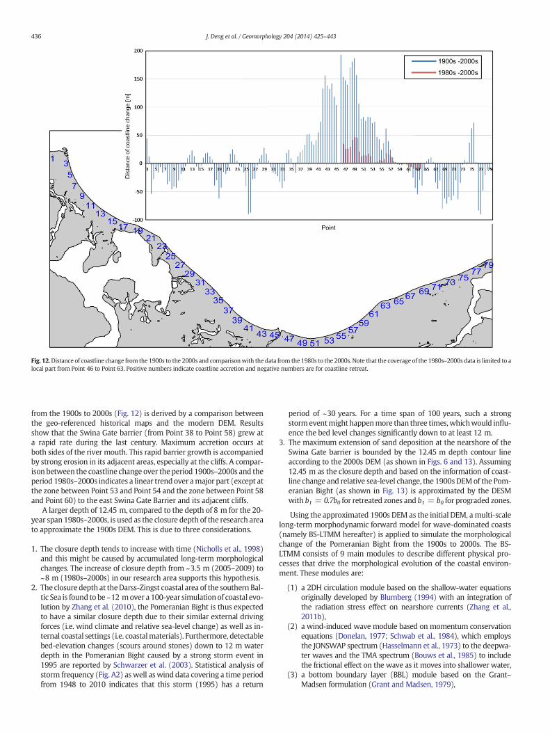
Fig. 12.Distance of coastline change from the 1900s to the 2000s and comparisonwith the data from the 1980s to the 2000s. Note that the coverage of the 1980s–2000s data is limited to alocal part from Point 46 to Point 63. Positive numbers indicate coastline accretion and negative numbers are for coastline retreat.

436 J. Deng et al. / Geomorphology 204 (2014) 425–443

from the 1900s to 2000s (Fig. 12) is derived by a comparison betweenthe geo-referenced historical maps and the modern DEM. Resultsshow that the Swina Gate barrier (from Point 38 to Point 58) grew ata rapid rate during the last century. Maximum accretion occurs atboth sides of the river mouth. This rapid barrier growth is accompaniedby strong erosion in its adjacent areas, especially at the cliffs. A compar-ison between the coastline change over the period 1900s–2000s and theperiod 1980s–2000s indicates a linear trendover amajor part (except atthe zone between Point 53 and Point 54 and the zone between Point 58and Point 60) to the east Swina Gate Barrier and its adjacent cliffs.

A larger depth of 12.45 m, compared to the depth of 8 m for the 20-year span 1980s–2000s, is used as the closure depth of the research areato approximate the 1900s DEM. This is due to three considerations.

1. The closure depth tends to increase with time (Nicholls et al., 1998)and this might be caused by accumulated long-term morphologicalchanges. The increase of closure depth from ~3.5 m (2005–2009) to~8 m (1980s–2000s) in our research area supports this hypothesis.

2. The closure depth at theDarss-Zingst coastal area of the southern Bal-tic Sea is found to be ~12 mover a 100-year simulation of coastal evo-lution by Zhang et al. (2010), the Pomeranian Bight is thus expectedto have a similar closure depth due to their similar external drivingforces (i.e. wind climate and relative sea-level change) as well as in-ternal coastal settings (i.e. coastalmaterials). Furthermore, detectablebed-elevation changes (scours around stones) down to 12 m waterdepth in the Pomeranian Bight caused by a strong storm event in1995 are reported by Schwarzer et al. (2003). Statistical analysis ofstorm frequency (Fig. A2) aswell aswind data covering a time periodfrom 1948 to 2010 indicates that this storm (1995) has a return

period of ~30 years. For a time span of 100 years, such a strongstormeventmight happenmore than three times,whichwould influ-ence the bed level changes significantly down to at least 12 m.

3. The maximum extension of sand deposition at the nearshore of theSwina Gate barrier is bounded by the 12.45 m depth contour lineaccording to the 2000s DEM (as shown in Figs. 6 and 13). Assuming12.45 m as the closure depth and based on the information of coast-line change and relative sea-level change, the 1900sDEMof the Pom-eranian Bight (as shown in Fig. 13) is approximated by the DESMwith b1 = 0.7b0 for retreated zones and b1 = b0 for prograded zones.

Using the approximated 1900s DEM as the initial DEM, a multi-scalelong-term morphodynamic forward model for wave-dominated coasts(namely BS-LTMM hereafter) is applied to simulate the morphologicalchange of the Pomeranian Bight from the 1900s to 2000s. The BS-LTMM consists of 9 main modules to describe different physical pro-cesses that drive the morphological evolution of the coastal environ-ment. These modules are:

(1) a 2DH circulation module based on the shallow-water equationsoriginally developed by Blumberg (1994) with an integration ofthe radiation stress effect on nearshore currents (Zhang et al.,2011b),

(2) a wind-induced wave module based on momentum conservationequations (Donelan, 1977; Schwab et al., 1984), which employsthe JONSWAP spectrum (Hasselmann et al., 1973) to the deepwa-ter waves and the TMA spectrum (Bouws et al., 1985) to includethe frictional effect on the wave as it moves into shallower water,

(3) a bottom boundary layer (BBL) module based on the Grant–Madsen formulation (Grant and Madsen, 1979),

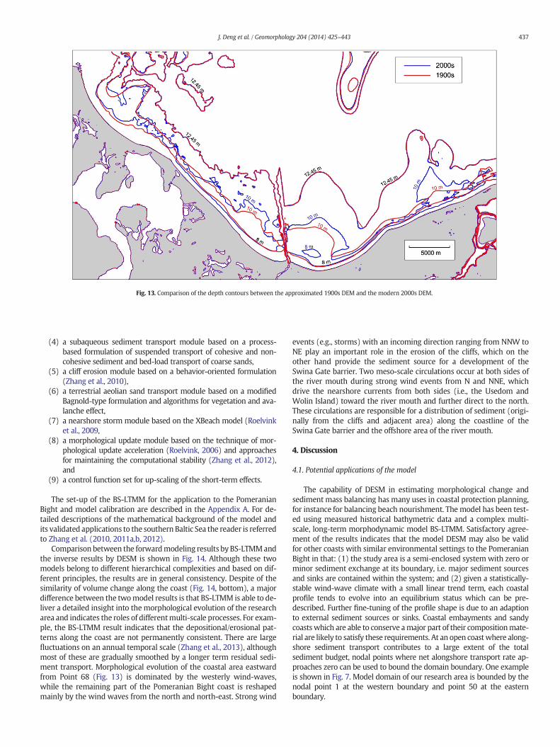
Fig. 13. Comparison of the depth contours between the approximated 1900s DEM and the modern 2000s DEM.

437J. Deng et al. / Geomorphology 204 (2014) 425–443

(4) a subaqueous sediment transport module based on a process-based formulation of suspended transport of cohesive and non-cohesive sediment and bed-load transport of coarse sands,

(5) a cliff erosion module based on a behavior-oriented formulation(Zhang et al., 2010),

(6) a terrestrial aeolian sand transport module based on a modifiedBagnold-type formulation and algorithms for vegetation and ava-lanche effect,

(7) a nearshore storm module based on the XBeach model (Roelvinket al., 2009,

(8) a morphological update module based on the technique of mor-phological update acceleration (Roelvink, 2006) and approachesfor maintaining the computational stability (Zhang et al., 2012),and

(9) a control function set for up-scaling of the short-term effects.

The set-up of the BS-LTMM for the application to the PomeranianBight and model calibration are described in the Appendix A. For de-tailed descriptions of the mathematical background of the model andits validated applications to the southern Baltic Sea the reader is referredto Zhang et al. (2010, 2011a,b, 2012).

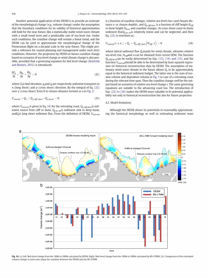
Comparison between the forwardmodeling results by BS-LTMMandthe inverse results by DESM is shown in Fig. 14. Although these twomodels belong to different hierarchical complexities and based on dif-ferent principles, the results are in general consistency. Despite of thesimilarity of volume change along the coast (Fig. 14, bottom), a majordifference between the twomodel results is that BS-LTMM is able to de-liver a detailed insight into the morphological evolution of the researcharea and indicates the roles of differentmulti-scale processes. For exam-ple, the BS-LTMM result indicates that the depositional/erosional pat-terns along the coast are not permanently consistent. There are largefluctuations on an annual temporal scale (Zhang et al., 2013), althoughmost of these are gradually smoothed by a longer term residual sedi-ment transport. Morphological evolution of the coastal area eastwardfrom Point 68 (Fig. 13) is dominated by the westerly wind-waves,while the remaining part of the Pomeranian Bight coast is reshapedmainly by the wind waves from the north and north-east. Strong wind

events (e.g., storms) with an incoming direction ranging from NNW toNE play an important role in the erosion of the cliffs, which on theother hand provide the sediment source for a development of theSwina Gate barrier. Two meso-scale circulations occur at both sides ofthe river mouth during strong wind events from N and NNE, whichdrive the nearshore currents from both sides (i.e., the Usedom andWolin Island) toward the river mouth and further direct to the north.These circulations are responsible for a distribution of sediment (origi-nally from the cliffs and adjacent area) along the coastline of theSwina Gate barrier and the offshore area of the river mouth.

4. Discussion

4.1. Potential applications of the model

The capability of DESM in estimating morphological change andsediment mass balancing has many uses in coastal protection planning,for instance for balancing beach nourishment. The model has been test-ed using measured historical bathymetric data and a complex multi-scale, long-term morphodynamic model BS-LTMM. Satisfactory agree-ment of the results indicates that the model DESM may also be validfor other coasts with similar environmental settings to the PomeranianBight in that: (1) the study area is a semi-enclosed system with zero orminor sediment exchange at its boundary, i.e. major sediment sourcesand sinks are contained within the system; and (2) given a statistically-stable wind-wave climate with a small linear trend term, each coastalprofile tends to evolve into an equilibrium status which can be pre-described. Further fine-tuning of the profile shape is due to an adaptionto external sediment sources or sinks. Coastal embayments and sandycoastswhich are able to conserve amajor part of their compositionmate-rial are likely to satisfy these requirements. At an open coastwhere along-shore sediment transport contributes to a large extent of the totalsediment budget, nodal points where net alongshore transport rate ap-proaches zero can be used to bound the domain boundary. One exampleis shown in Fig. 7. Model domain of our research area is bounded by thenodal point 1 at the western boundary and point 50 at the easternboundary.

438 J. Deng et al. / Geomorphology 204 (2014) 425–443

Another potential application of the DESM is to provide an estimateof themorphological change (e.g., volume change) under the assumptionthat the boundary conditions for its validity of historical approximationstill hold for the near-future, like a statistically-stable wind-wave climatewith a small trend term and a predictable rate of sea-level rise. Undersuch conditions, the coastline change will remain a linear trend, and theDESM can be used to approximate the morphological change of thePomeranian Bight on a decadal scale in the near-future. This might pro-vide a reference for coastal planning and management under such strictconditions. However, the projection by DESM on future coastline changebased on scenarios of sea-level change orwind climate change is also pos-sible, provided that a governing equation for bed level change (Roelvinkand Reniers, 2012) is introduced:

∂Zb

∂t þ ∂qx∂x þ ∂qy

∂y ¼ 0 ð22Þ

where Zbis bed elevation, qxand qyare respectively sediment transports inx-(long shore) and y-(cross shore) direction. By the integral of Eq. (22)over y (cross shore) from 0 to closure distance termed as x*in Fig. 2:

Vexternal þ Qx þ Qy;cliff =dune−Qy;ba sin ¼ 0 ð23Þ

where Vexternal is given in Eq. (4) for the retreating coast, Qy,cliff/duneis sed-iment source from cliff or dune, Qy,ba sinis sediment sink to deep basin,andQxis long shore sediment flux. From the definition of DESM, Vexternal

Fig. 14. (a) Left: Bed-level change from the 1900s to 2000s calculated byDESM; Right: Bed-levelvolume change in each zone along the coastline between the DESM and the BS-LTMM.

is a function of coastline changec, relative sea-level rise s and closure dis-tance x* or closure depthh*, and Qy,cliff/dune is a function of cliff height Hcliff

or dune heightHdune and coastline changec. As cross-shore coast-to-basinsediment fluxQy,ba sinis relatively minor and can be neglected, and thenEq. (23) is rewritten as:

Vexternal c; s; x�ð Þ þ Qx þ Qy;cliff =dune Hcliff ; c� �

¼ 0 ð24Þ

where lateral sediment flux Qxstands for wind climate, sdenotes relativesea-level rise, Hcliffand x*can be obtained from recent DEM. The functionQy,cliff/dunecan be easily determined by Eqs. (13), (14) and (15), and thefunction Vexternalshould be able to be determined by least squared regres-sion on historical reconstruction data by DESM. The assumption of sta-tionary wind-wave climate in the future allows Qx to be approximatelyequal to the historical sediment budget. The latter one is the sum of ero-sion volume and deposition volume in Fig. 3 in case of a retreating coastduring the relevant time span. Then the coastline change cwill be the out-put based on scenarios of relative sea-level change s. The same governingequations are suitable to the advancing coast too. The introduction ofEqs. (22) to (24) makes the DESMmore valuable in its potential applica-bility not only in historical reconstruction but also for future projection.

4.2. Model limitations

Although the DESM shows its potentials in reasonably approximat-ing the historical morphology as well as estimating sediment mass

change from the1900s to 2000s calculated byBS-LTMM; (b): Comparison of the calculated

439J. Deng et al. / Geomorphology 204 (2014) 425–443

balancing of the Pomeranian Bight on a decadal-to-centennial temporalscale, some shortcomings of the approach deserve further discussions.Three limitations of the approach make its universal applicability forgeneral coastal environments require considerable caution. The first isthat the study area must be a semi-enclosed system of sediment trans-port like coastal embayment areas which cannot be satisfied at manyopen boundary coasts where net transport (either income or outcome)of sediment at the boundary always exist. Therefore, the investigationon sediment source-to-sink transport needs to be carried out before ap-plying this model. For this investigation, the longshore sediment trans-port capacity model is a useful tool for estimating net lateral sedimentflux at the boundary. In additoon, the investigation on the sink of sedi-ment source from river is also required. For example, Fig. 7 indicatesthat the Swina river mouth is the convergence of sediment sourcesfrom coastal erosion, and the sand from river deposits only at the vicin-ity of the river mouth and covers less than 5% of the total area.

The second limitation is that there are several sources for certainpossible error of the model. As expected, the occurrence of the regularpattern of bed level change by DESM (Fig. 14) is due to the mathemat-ical description that is based on generalized Bruun rule model in defin-ing the change of the coastal profile shape. This shows its uncertainty inreflectingmore complex processes that can beproducedbymechanical-ly process-based, long-term morphodynamic model. An example todemonstrate such limitation is in point 57 of Fig. 14(a). Here, small-scale structures such as multiple longshore bars are not taken into ac-count. This may also introduce errors into the estimation of sedimentbudget along the profile. The second source of error comes from the ac-curacy of historical maps. Coastline change is actually a crucial elementof the model, as it mainly determines the eroded and accumulated sed-iment mass volume, respectively, for the retreated and advancing coastin themodel, with the adaptation of coastal profile shape to balance thetotal sediment budget by the inverse procedure. Another source of errorcomes from an adoption of a uniform closure depth for the whole studyarea in a given temporal scale. In local parts of the coastwhere sedimenttransport is influenced by some specific processes, for instance, in thevicinity of a river mouth, profiles normally have different closuredepth with other parts of the coast. Profile measurements from 2005to 2009 in our research area indicate such variability in the closuredepth (Zhang et al., 2013). In the application of the DESM at the Pomer-anian Bight, these sources of error account for ~20% of the total sedi-ment budget from the measured historical nautical chart data andmore complex model BS-LTMM. Among the total error, the mathemat-ical description of generalized Bruun rule model are a major source oferror, as can be seen in Figs. 10 and 14, and the approximated closuredepth is a secondary source of error.

The third limitation is a lack of a precise quantifying method to de-termine the closure depth that varies with different time span andlong-term hydrodynamic environment. For example, 8 m for the 20-year period and 12.45 m for the 100-year period is assumed uniformalong the coast at the Pomeranian Bight. But the results indicate that12.45 m closure depth is reasonable from the pattern of bed levelchanges shown in Fig. 14(a), except that in the vicinity of Swina rivermouth the closure depth appears to be larger than 12.45 m. The estima-tion of the closure depth can also be obtained by previous results fromnearby areawith similar external driving forces and internal coastal set-tings. The consequence of misuse of closure depth can be severe, as theprofile slope is approaching zero at the concave coastal profile (Fig. 1) inwhich 2 m of closure depth change can make the closure distance de-crease by more than 50%. In the Pomeranian Bight for the 100-year pe-riod, 10.45 m closure depth instead of 12.45 m reduces the totalsediment budget calculated by DESM by ~54% and 11.45 m closuredepth reduces the total sediment budget by ~28%. Therefore, the impactof the selection of closure depth on the results must be taken into ac-count seriously. A further improvement of the DESM may be achievedby developing a precise quantifying method for the closure depth thatvaries along the coast and depends on the local long-term effect of the

wind-wave strength. Considering the limitations of the approach men-tioned above, the boundary conditions of the system must be studiedcarefully before applying DESM.

5. Conclusions

A numerical approach for approximation of the historical mor-phology of wave-dominated coasts is presented in this study. The ap-proach, namely the Dynamic Equilibrium Shore Model (DESM), usesthe historical coastline configuration, a high-resolution modern DEMand relative sea-level change to approximate the historical DEM of thestudy area in the case of insufficient survey data. The basic concept ofthe approach is a dynamic equilibrium of the coastal cross-shore profileshape resulting from an adaptation to external sediment sources orsinks, under the pre-condition that the main driving force is stable with-out notable changes on the scale of interest. The approach demonstratesits applicability in an approximation of the historical morphology of thePomeranian Bight (southern Baltic Sea) for the 1980s, in which thedepositional/erosional patterns and volume change along the coastlineshow good agreement with measurement data. The 8 m and 12.45 mdepth contour as an indicator of closure depth may also be valid forother parts of the southern Baltic Sea for a time span of ~20 years and~100 years, respectively. Another potential of the approach is that theapproximated historical morphology of a study area may serve as thestarting point as well as calibration measures for complex long-term,morphodynamic forwardmodels. The approximated historical morphol-ogy of the Pomeranian Bight for the 1900s by the approach serves as theinitial DEM for a complex morphodynamic forward model to deliver adetailed insight into the morphological evolution of the system, inwhich the roles of multi-scale physical processes are revealed. This indi-cates that the DESM can serve as a useful tool for coastal morphologicalstudies. The approach applies also for other coastal environments provid-ed that the pre-conditions are met. The approach can also be used to es-timate a near-future change of the coastal morphology based on anassumption of a linear trend in the boundary conditions. It has also a po-tential application to project coastline change based on scenarios of sea-level rise by assuming a stationarywind-wave climate in the near-future.

Acknowledgments

The study is supported by the CoPaF project funded by the PolishMinistry of Science andHigher Education and theBaltic Network projectfunded by the Ernst-Moritz-Arndt University of Greifswald, Germany.The historical ‘Messtischblatt’ maps are provided by the University ofGreifswald (for the German part of the Pomeranian Bight) and the Uni-versity of AdamMickiewicz in Poznan (for the Polish part of the Pomer-anian Bight). The authors also thank the Narodowe Centrum Nauki(NCN) for financial support of this study (No. DEC-2011/01/N/ST10/07531).We greatly appreciate the comments from the editor and anon-ymous reviewers, which were helpful for the improvement of thispaper.

Appendix A

1. Set-up of BS-LTMM for the research area

Using the approximated 1900s DEM as the starting point, a multi-scale morphodynamic forward model (BS-LTMM) is applied to recon-struct the morphological evolution of the Pomeranian Bight coast fromthe 1900s to the 2000s. Parameter settings of the model are calibratedby the coastline change from the 1980s to the 2000s, for which experi-mental runs were performed to test the sensitivity of the model resultsto different settings of boundary inputs. Somekey settings for themodelapplication are presented here:

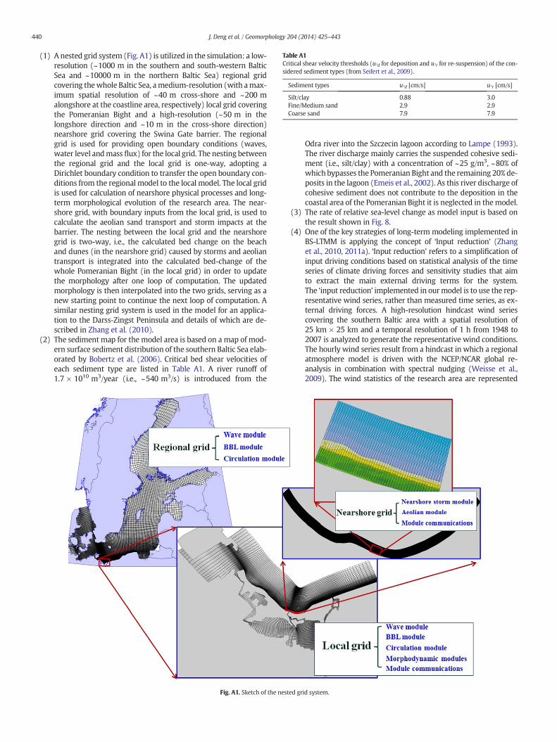
Table A1Critical shear velocity thresholds (u*d for deposition and u*r for re-suspension) of the con-sidered sediment types (from Seifert et al., 2009).

Sediment types u*d [cm/s] u*r [cm/s]

Silt/clay 0.88 3.0Fine/Medium sand 2.9 2.9Coarse sand 7.9 7.9

440 J. Deng et al. / Geomorphology 204 (2014) 425–443

(1) A nested grid system (Fig. A1) is utilized in the simulation: a low-resolution (~1000 m in the southern and south-western BalticSea and ~10000 m in the northern Baltic Sea) regional gridcovering thewhole Baltic Sea, amedium-resolution (with amax-imum spatial resolution of ~40 m cross-shore and ~200 malongshore at the coastline area, respectively) local grid coveringthe Pomeranian Bight and a high-resolution (~50 m in thelongshore direction and ~10 m in the cross-shore direction)nearshore grid covering the Swina Gate barrier. The regionalgrid is used for providing open boundary conditions (waves,water level andmass flux) for the local grid. The nesting betweenthe regional grid and the local grid is one-way, adopting aDirichlet boundary condition to transfer the open boundary con-ditions from the regional model to the local model. The local gridis used for calculation of nearshore physical processes and long-term morphological evolution of the research area. The near-shore grid, with boundary inputs from the local grid, is used tocalculate the aeolian sand transport and storm impacts at thebarrier. The nesting between the local grid and the nearshoregrid is two-way, i.e., the calculated bed change on the beachand dunes (in the nearshore grid) caused by storms and aeoliantransport is integrated into the calculated bed-change of thewhole Pomeranian Bight (in the local grid) in order to updatethe morphology after one loop of computation. The updatedmorphology is then interpolated into the two grids, serving as anew starting point to continue the next loop of computation. Asimilar nesting grid system is used in the model for an applica-tion to the Darss-Zingst Peninsula and details of which are de-scribed in Zhang et al. (2010).

(2) The sediment map for the model area is based on a map of mod-ern surface sediment distribution of the southern Baltic Sea elab-orated by Bobertz et al. (2006). Critical bed shear velocities ofeach sediment type are listed in Table A1. A river runoff of1.7 × 1010 m3/year (i.e., ~540 m3/s) is introduced from the

Fig. A1. Sketch of the n

Odra river into the Szczecin lagoon according to Lampe (1993).The river discharge mainly carries the suspended cohesive sedi-ment (i.e., silt/clay) with a concentration of ~25 g/m3, ~80% ofwhich bypasses the Pomeranian Bight and the remaining 20%de-posits in the lagoon (Emeis et al., 2002). As this river discharge ofcohesive sediment does not contribute to the deposition in thecoastal area of the Pomeranian Bight it is neglected in themodel.

(3) The rate of relative sea-level change as model input is based onthe result shown in Fig. 8.

(4) One of the key strategies of long-term modeling implemented inBS-LTMM is applying the concept of ‘Input reduction’ (Zhanget al., 2010, 2011a). ‘Input reduction’ refers to a simplification ofinput driving conditions based on statistical analysis of the timeseries of climate driving forces and sensitivity studies that aimto extract the main external driving terms for the system.The ‘input reduction’ implemented in ourmodel is to use the rep-resentative wind series, rather than measured time series, as ex-ternal driving forces. A high-resolution hindcast wind seriescovering the southern Baltic area with a spatial resolution of25 km × 25 km and a temporal resolution of 1 h from 1948 to2007 is analyzed to generate the representative wind conditions.The hourly wind series result from a hindcast in which a regionalatmosphere model is driven with the NCEP/NCAR global re-analysis in combination with spectral nudging (Weisse et al.,2009). The wind statistics of the research area are represented

ested grid system.

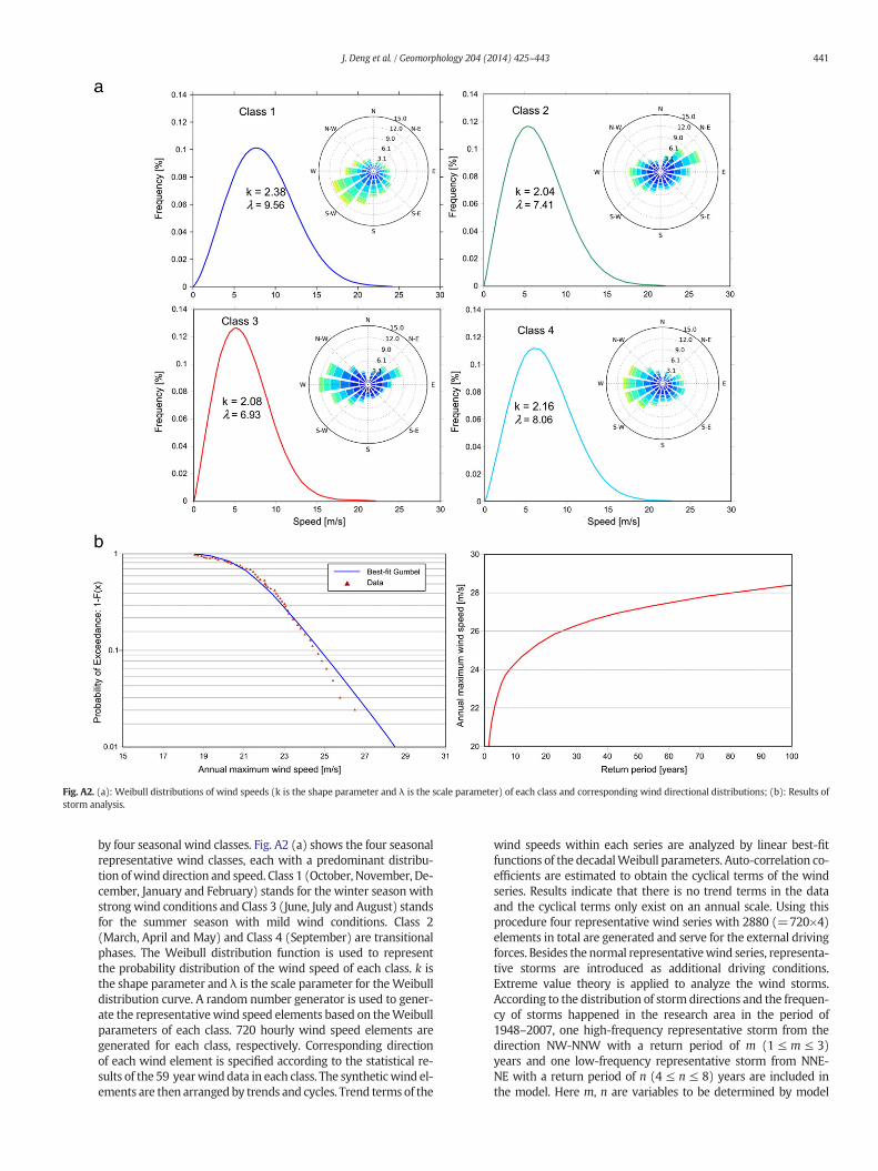
Fig. A2. (a): Weibull distributions of wind speeds (k is the shape parameter and λ is the scale parameter) of each class and corresponding wind directional distributions; (b): Results ofstorm analysis.

441J. Deng et al. / Geomorphology 204 (2014) 425–443

by four seasonal wind classes. Fig. A2 (a) shows the four seasonalrepresentative wind classes, each with a predominant distribu-tion ofwind direction and speed. Class 1 (October, November, De-cember, January and February) stands for the winter season withstrongwind conditions and Class 3 (June, July and August) standsfor the summer season with mild wind conditions. Class 2(March, April and May) and Class 4 (September) are transitionalphases. The Weibull distribution function is used to representthe probability distribution of the wind speed of each class. k isthe shape parameter and λ is the scale parameter for theWeibulldistribution curve. A random number generator is used to gener-ate the representativewind speed elements based on theWeibullparameters of each class. 720 hourly wind speed elements aregenerated for each class, respectively. Corresponding directionof each wind element is specified according to the statistical re-sults of the 59 yearwinddata in each class. The syntheticwind el-ements are then arrangedby trends and cycles. Trend terms of the

wind speeds within each series are analyzed by linear best-fitfunctions of the decadalWeibull parameters. Auto-correlation co-efficients are estimated to obtain the cyclical terms of the windseries. Results indicate that there is no trend terms in the dataand the cyclical terms only exist on an annual scale. Using thisprocedure four representative wind series with 2880 (=720×4)elements in total are generated and serve for the external drivingforces. Besides the normal representativewind series, representa-tive storms are introduced as additional driving conditions.Extreme value theory is applied to analyze the wind storms.According to the distribution of storm directions and the frequen-cy of storms happened in the research area in the period of1948–2007, one high-frequency representative storm from thedirection NW-NNW with a return period of m (1 ≤ m ≤ 3)years and one low-frequency representative storm from NNE-NE with a return period of n (4 ≤ n ≤ 8) years are included inthe model. Here m, n are variables to be determined by model

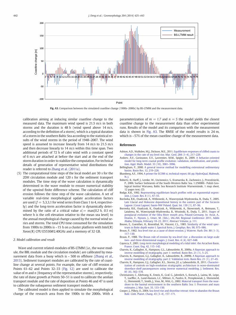
Fig. A3. Comparison between the simulated coastline change (1900s–2000s) by BS-LTMM and the measurement data.

442 J. Deng et al. / Geomorphology 204 (2014) 425–443

calibration aiming at inducing similar coastline change to themeasured data. The maximum wind speed is 21.5 m/s in bothstorms and the duration is 48 h (wind speed above 14 m/s,according to the definition of a storm), which is a typical durationof a storm in the southern Baltic Sea according to the statistical re-sults of the wind storms in the period of 1948–2007. The windspeed is assumed to increase linearly from 14 m/s to 21.5 m/sand then decrease linearly to 14 m/s within this time span. Twoadditional periods of 72 h of calm wind with a constant speedof 6 m/s are attached at before the start and at the end of thestormduration in order to stabilize the computation. For technicaldetails of generation of representative wind distributions thereader is referred to Zhang et al. (2011a).

(5) The computational time steps of the local model are 30 s for the2DH circulation module and 120 s for the sediment transportmodules. The time step of the wave calculation is dynamicallydetermined in the wave module to ensure numerical stabilityof the upwind finite difference scheme. The calculation of clifferosion follows the time step of the wave calculation. A set ofvariable real-time morphological update acceleration factorsare used (f = 5,3,3,1 forwind series fromClass 1 to 4, respective-ly) and the long-term acceleration factor is dynamically deter-mined by the ratio of a critical value ε(= max{0.2 h, 0.5 m}where h is the cell elevation relative to the mean sea level) tothe annualmorphological change caused by the normal wind se-ries and storms. The total CPU time consumed for the simulationfrom 1900s to 2000s is ~15 h on a cluster platform with Intel(R)Xeon(R) CPU E5530@2.40GHz and a memory of 32 GB.

2. Model calibration and result

Wave and current related-modules of BS-LTMM (i.e., thewavemod-ule, the BBLmodule and the circulation module) are calibrated bymea-surement data from a buoy which is ~ 500 m offshore (Zhang et al.,2013). Sediment transport modules are calibrated by the rate of coast-line change at several points. For example, the rate of cliff erosion atPoints 61–62 and Points 32–33 (Fig. 12) are used to calibrate thevalue ofm and n (frequency of the representative storms), respectively;the rate of dune growth at Points 50–51 is used to calibrate the aeoliantransport module and the rate of deposition at Points 46 and 47 is usedto calibrate the subaqueous sediment transport modules.

The calibrated model is then applied to simulate the morphologicalchange of the research area from the 1900s to the 2000s. With a

parameterization of m = 1.7 and n = 5 the model yields the closestcoastline change to the measurement data than other experimentalruns. Results of the model and its comparison with the measurementdata is shown in Fig. A3. The RMSE of the model results is 24 m,which is ~57% of the mean coastline change of the measurement data.

References

Ashton, A.D., Walkden, M.J., Dickson, M.E., 2011. Equilibrium responses of cliffed coasts tochanges in the rate of sea level rise. Mar. Geol. 284 (1–4), 217–229.

Avdeev, A.V., Goriounov, E.V., Lavrentiev, M.M., Spigler, R., 2009. A behavior-orientedmodel for long-term coastal profile evolution: validation, identification, and predic-tion. Appl. Math. Model. 33 (10), 3981–3996.

Bellingham, P., 2000. A general inverse method for modelling extensional sedimentarybasins. Basin Res. 12, 219–226.

Blumberg, A.F., 1994. A primer for ECOM-si, technical report, 66 pp. HydroQual, Mahwah,N. J.

Bobertz, B., Harff, J., Lemke, W., Uscinowicz, S., Kramarska, R., Zachowicz, J., Przezdziecki,P., 2006. Surface Sediments of the South-Western Baltic Sea. 1:250000.- Polish Geo-logical Institut Warsawa, Baltic Sea Research Institute Warnemünde, 1 map sheet,12 pages text, CD.

Bodge, K.R., 1992. Representing equilibrium beach profiles with an exponential expres-sion. J. Coast. Res. 8 (1), 47–55.

Borówka, R.K., Osadczuk, A., Witkowski, A., Wawrzyniak-Wydrowska, B., Duda, T., 2005.Late Glacial and Holocene depositional history in the eastern part of the SzczecinLagoon (Great Lagoon) basin-NW Poland. Quat. Int. 130 (1), 87–96.

Borowka, R.K., Osadczuk, K., Osadczuk, A., Witkowski, A., Skowronek, A., Reimann, T.,Latalowa, M., Wawrzyniak-Wydrowska, B., Wozinski, R., Duda, T., 2011. Stages ofpostglacial evolution of the Odra River mouth area, Poland-Germany. In: Asrat, A.,Dramis, F., Nyssen, J., Umer, M. (Eds.), IAG/AIG Regional Conference 2011, AddisAbaba, Ethiopia, February 18–22, 2011; Abstract Volume, p. 111.

Bouws, E., Guenther, H., Rosenthal, W., Vincent, C.L., 1985. Similarity of the wind spec-trum in finite depth water I. Spectral form. J. Geophys. Res. 90, 975–986.

Bruun, P., 1962. Sea-level rise as a cause of shore erosion. J. Waterw. Harb. Div. 88 (1–3),117–130.

Bruun, P., 1988. The Bruun rule of erosion by sea-level rise: a discussion on large-scaletwo- and three-dimensional usages. J. Coast. Res. 4 (4), 627–648.

Cayocca, F., 2001. Long-term morphological modeling of a tidal inlet: the Arcachon Basin,France. Coast. Eng. 42, 115–142.

Charvin, K., Gallagher, K., Hampson, G.L., Labourdette, R., 2009a. A Bayesian approach toinverse modelling of stratigraphy, part 1: method. Basin Res. 21 (1), 5–25.

Charvin, K., Hampson, G.J., Gallagher, K., Labourdette, R., 2009b. A Bayesian approach toinverse modelling of stratigraphy, part 2: Validation tests. Basin Res. 21 (1), 27–45.

Charvin, K., Hampson, G.J., Gallagher, K.L., Storms, J.E. a, Labourdette, R., 2011. Character-ization of controls on high-resolution stratigraphic architecture in wave-dominatedshoreface-shelf parasequences using inverse numerical modeling. J. Sediment. Res.81 (8), 562–578.

Christiansen, C., Edelvang, K., Emeis, K., Graf, G., Jahmlich, S., Kozuch, J., Laima, M., Leipe,T., Loeffler, A., Lund-Hansen, L.C., Miltner, A., Pazdro, K., Pempkowiak, J., Shimmield,G., Shimmield, T., Smith, J., Voss, M., Witt, G., 2002. Material transport from the near-shore to the basinal environment in the southern Baltic Sea: I: Processes and massestimates. J. Mar. Syst. 35, 133–150.

Cooper, J., Pilkey, O., 2004. Sea-level rise and shoreline retreat: time to abandon the BruunRule. Glob. Planet. Chang. 43 (3–4), 157–171.

443J. Deng et al. / Geomorphology 204 (2014) 425–443

Cowell, P., Roy, P.S., Jones, R.A., 1995. Simulation of large-scale coastal change using amorphological behaviour model. Mar. Geol. 126 (1–4), 45–61.

Cross, T., Lessenger, M., 1999. Construction and application of a stratigraphic inversemodel. In: Harbaugh, J., Watney, W., Rankey, E., Slingerland, R., Goldstein, R.,Franseen, E. (Eds.), SEPM Special Publication 62: Numerical Experiments in Stratigra-phy: Recent Advances in Stratigraphic and Sedimentologic Computer Simulations.SEPM (Society for Sedimentary Geology), pp. 69–83.

Dastgheib, A., Roelvink, J.A., Wang, Z.B., 2008. Long term process-based morphologicalmodelling of the Marsdiep tidal basin. Mar. Geol. 256, 90–100.

Davidson-Arnott, R.G.D., 2005. Conceptual model of the effects of sea level rise on sandycoasts. J. Coast. Res. 216 (216), 1166–1172.

Dean, R.G., 1991. Equilibrium beach profiles: characteristics and applications. J. Coast. Res.7 (1), 53–84.

Deng, J., Dudzinska-Nowak, J., Giza, A., Terefenko, P., Zhang, W., 2011. Monitoring ofcoastal changes in the Pomeranian Bay, southern Baltic Sea—a methodologicalapproach. LOICZ Open Science Conference “Coastal Systems, Global Change andSustainability”. Yantai, China, p. 109.

Diesing, M., Furmanczyk, K., Hanson, H., Niedermeyer, R.-O., Pruszak, Z., 1999. Presentfluxes of inorganic matter in Pomeranian Bay. 3rd BASYS Final Conference. Institutfür Ostseeforschung Warnemünde. http://www.io-warnemuende.de/Projects/Basys/bio/con3/con3top.htm#T2-10.

Donelan, M., 1977. A simple numerical model for wave and wind stress application.Report. , 28. National Water Research Institute, Burlington.

Emeis, K., Christiansen, C., Edelvang, K., Graf, G., Jahmlich, S., Kozuch, J., Laima, M.,Leipe, T., Loeffler, A., Lund-Hansen, L.C., Miltner, A., Pazdro, K., Pempkowiak, J.,Shimmield, G., Shimmield, T., Smith, J., Voss, M., Witt, G., 2002. Material trans-port from the near shore to the basinal environment in the southern Baltic Sea:II. Synthesis of data on origin and properties of material. J. Mar. Syst. 35 (3–4),151–168.

Froehle, P., Dimke, S., 2008. Sediment transport at the Coast of Mecklenburg-Vorpommern,Germany. In: Smith, J.M. (Ed.), Proceedings of the 31st international conference onCoastal Engineering, Vol. 3. Hamburg, Germany, pp. 2471–2480.

Furmanczyk, K., Dudzinska-Nowak, J., 2009. Extreme Storm Impact to the coastlinechanges—South Baltic example. Journal of Coastal Research. SI 56 (Proceedings ofthe 10th International Coastal Symposium), pp. 1637–1640.

Grant, W.D., Madsen, O.S., 1979. Combined wave and current interaction with a roughbottom. J. Geophys. Res. 84, 1797–1808.

Harff, J., Lüth, F., 2007. In: Harff, J., Lüth, F. (Eds.), Sinking Coasts—Geosphere Ecosphereand Anthroposphere of the Holocene Southern Baltic Sea. Rep. Roman GermanicCommission.

Harff, J., Meyer, M., 2011. Coastlines of the Baltic Sea—zones of competition betweengeological processes and a changing climate: examples from the Southern Baltic—Springer. In: Harff, J., Björck, S., Hoth, P. (Eds.), The Baltic Sea Basin. Springer-Verlag,Berlin, Heidelberg, pp. 149–164.

Hasselmann, K., Barnett, T.P., Bouws, E., Carlson, H., Cartwright, D.E., Enke, K., Ewing, J.A.,et al., 1973. Measurements of wind-wave growth and swell decay during the JointNorth Sea Wave Project (JONSWAP). , Vol. 95. Deutsche Hydrographische Zeitschrift,Erganzungs-ft.

Hesp, P.A., Martinez, M.L., 2007. Disturbance processes and dynamics in coastal dunes—academic. In: Johnson, E.A., Miyanishi, K. (Eds.), Plant Disturbance Ecology. Academic,San Diego, pp. 215–247.

IPCC, 2007. Climate change 2007: the physical science basis. In: Solomon, S., Qin, D.,Manning, M., Chen, Z., Marquis, M., Averyt, K.B., Tignor, M., Miller, H.L. (Eds.), Contri-bution ofWorking Group I to the Fourth Assessment Report of the IntergovernmentalPanel on Climate Change. Cambridge University Press, Cambridge.

Jimenez, J.A., Arcilla, A.S., 2004. A long-term (decadal scale) evolution model formicrotidal barrier systems. Coast. Eng. 51, 749–764.

Karunarathna, H., Reeve, D., Spivack, M., 2008. Long-term morphodynamic evolution ofestuaries: an inverse problem. Estuarine Coastal Shelf Sci. 77 (3), 385–395.

Keilhack, K., 1912. Die Verlandung der Swinepforte. Jahrbuch der Königliche-PreussischenGeologischen Landesanstalt, XXXII 209–244.

Komar, P.D., Mcdougal, W.G., 1994. The analysis of exponential beach profiles. J. Coast.Res. 10 (1), 59–69.

Labuz, T., 2005. Present-day dune environment dynamics on the coast of the Swina GateSandbar (Polish West coast). Estuarine Coastal Shelf Sci. 62, 507–520.

Lampe, R., 1993. Environmental state and material flux in the western part of the Oderriver estuary—results and consequences. Petermanns Geogr. Mitt. 137 (1993/5),275–282.

Leipe, T., Eidam, J., Lampe, R., Meyer, H., Neumann, T., Osadczuk, A., Janke, W., Puff, T.,Blanz, T., Gingele, F.X., Dannenberger, D., Witt, G., 1998. Das Oderhaff. Beiträge zur

Rekonstruktion der holozänen geologischen Entwicklung und anthropogenenBeein-flussung des Oder-Ästuars. Mar. Sci. Rep. 28, 1–28.

Musielak, S., Osadczuk, K., 1995. Evolution of the Swina Gate. In: Rotnicki, K. (Ed.), Journalof Coastal Research, Special Issue. , 22. CERF (USA), pp. 305–308.

Nicholls, R., Birkemeier,W.A., Lee, G., 1998. Evaluation of depth of closure using data fromDuck, NC, USA. Mar. Geol. 148 (3–4), 179–201.

Pilkey, O., Cooper, J., 2004. Society and sea level rise. Science 303, 1781–1782.Piotrowski, A., 1999. Etapy rozwoju Bramy Świny. In: Borówka, R.K., Piotrowski, A.,

Wiśniowski, Z. (Eds.), Problemy geologii, hydrogeologii i ochrony środowiska wybrzeżamorskiego Zachodniego Pomorza. Przewodnik LXX Zjazdu Naukowego PTG, Szczecin,pp. 215–241.

Pruszak, Z., 2003. Akweny morskie. Zarys procesów fizycznych i inżynierii środowiska.IBW PAN, Gdańsk.

Psuty, N.P., 1988. Sediment budget and dune/beach interaction. J. Coast. Res. Spec. Issue 3,1–4.

Roelvink, J., 2006. Coastal morphodynamic evolution techniques. Coast. Eng. 53 (2–3),277–287.

Roelvink, Dano, Reniers, Ad, 2012. A Guide toModeling CoastalMorphology.World Scien-tific Publishing, Singapore 111–143.

Roelvink, D., Reniers, A., van Dongeren, A., van Thiel de Vries, J., McCall, R., Lescinski, J.,2009. Modelling storm impacts on beaches, dunes and barrier islands. Coast. Eng.56 (11–12), 1133–1152.

Schwab, D., Bennett, J., Liu, P., Donelan, M., 1984. Application of a simple numerical waveprediction model to lake Erie. J. Geophys. Res. 89, 3586–3592.

Schwarzer, K., Diesing, M., Larson, M., Niedermeyer, R.-O., Schumacher, W., Furmańczyk,K., 2003. Coastline evolution at different time scales—examples from the PomeranianBight, southern Baltic Sea. Mar. Geol. 194, 79–101.

SCOR, 1991. The response of beaches to sea-level changes: a review of predictive models.J. Coast. Res. 7, 895–921.

Seifert, T., Fennel, W., Kuhrts, C., 2009. High resolution model studies of transport of sed-imentary material in the south-western Baltic. J. Mar. Syst. 75, 382–396.

Soomere, T., Viska, M., Lapinskis, J., Raamet, A., 2011. Linking wave loads with the inten-sity of erosion along the coasts of Latvia. Estonian J. Eng. 17 (4), 359–374.

Spivack, M., Reeve, D.E., 2000. Source reconstruction in a coastal evolution equation.J. Comput. Phys. 161 (1), 169–181.

Tarantola, A., 1987. Inverse Problem Theory. Elsevier, Amsterdam.Thieler, E.R., Pilkey Jr., O.H., Young, R.S., Bush, D.M., Chai, F., 2000. The use of mathematical

models to predict beach behavior for U.S. coastal engineering: a critical review.J. Coast. Res. 16 (1), 48–70.

U.S. Army Corps of Engineers, 1984. Shore Protection Manual, 4th ed. Department of theArmy, U.S. Corps of Engineers, Washington, DC.

Weisse, R., v. Storch, H., Callies, U., Chrastansky, A., Feser, F., Grabemann, I.,Guenther, H., Pluess, A., Stoye, T., Tellkamp, J., Winterfeldt, J., Woth, K., 2009.Regional meteo-marine reanalyses and climate change projections: resultsfor Northern Europe and potentials for coastal and offshore applications. Bull.Am. Meteorol. Soc. 90, 849–860.

Wijns, C., Boschetti, F., Moresi, L., 2003. Inverse modelling in geology by interactiveevolutionary computation. J. Struct. Geol. 25, 1615–1621.

Wolinsky, M. a, Murray, a.B., 2009. A unifying framework for shoreline migration: 2.Application to wave-dominated coasts. J. Geophys. Res. 114 (F1), 1–13.

Wu, C.Y., Ren, J., Bao, Y., Lei, Y.P., Shi, H.Y., He, Z.G., 2007. A long-term hybrid morpholog-ical modeling study on the evolution of the Pearl River delta, network system andestuarine bays since 6000 aBP. In: Harff, J., Hay, W.W., Tetzlaff, D.F. (Eds.), CoastlineChanges: Interrelation of Climate and Geological Processes. Geological Society ofAmerica, Special Paper, 46, pp. 199–214.

Zawadzka-Kahlau, E., 1999. Development Tendencies of the Polish South Baltic Coast(in Polish). Gdanskie Towarzystwo Naukowe, Gdansk.

Zhang, W.Y., Harff, J., Schneider, R., Wu, C.Y., 2010. Development of a modeling method-ology for simulation of long-term morphological evolution of the southern Balticcoast. Ocean Dyn. 60 (5), 1085–1114.

Zhang, W.Y., Harff, J., Schneider, R., 2011a. Analysis of 50-year wind data of the southernBaltic Sea for modelling coastal morphological evolution—a case study from theDarss-Zingst Peninsula. Oceanologia 53, 489–518.

Zhang,W.Y., Harff, J., Schneider, R.,Wu, C.Y., 2011b. Amulti-scale centennialmorphodynamicmodel for the southern Baltic coast. J. Coast. Res. 27, 890–917.

Zhang, W.Y., Schneider, R., Harff, J., 2012. A multi-scale hybrid long-termmorphodynamicmodel for wave-dominated coasts. Geomorphology 149–150, 49–61.

Zhang, W.Y., Deng, J., Harff, J., Schneider, R., Dudzinska-nowak, J., 2013. A coupled model-ing scheme for longshore sediment transport of wave-dominated coasts—a casestudy from the southern Baltic Sea. Coast. Eng. 72, 39–55.