V

MA

a

ARRA

1

mtcp2tR

so(wdHfiwa

0d

Nuclear Engineering and Design 241 (2011) 2075–2085

Contents lists available at ScienceDirect

Nuclear Engineering and Design

journa l homepage: www.e lsev ier .com/ locate /nucengdes

ery-Large Eddy Simulation (V-LES) of the flow across a tube bundle

athieu Labois, Djamel Lakehal ∗

SCOMP GmbH, Technoparkstrasse 1, CH-8005 Zürich, Switzerland

r t i c l e i n f o

rticle history:eceived 14 September 2010eceived in revised form 15 February 2011ccepted 18 February 2011

a b s t r a c t

A new turbulence modelling approach (Very-Large Eddy Simulation; V-LES) is developed and compared toconventional RANS and LES for a flow across a tube bundle. The method, which belongs to the large-scalesimulation category, represents a good compromise between efficiency and precision, and may thus beused for industrial problems for which LES remains computationally expensive under high to very-highReynolds number flow conditions. It can also be used for gas–liquid two-phase flows such as pressurizedthermal shocks. The method is a sort of blend between U-RANS and LES, in that it resolves very largestructures – way larger than the grid size – and models all subscale of turbulence using a two-equationmodel, by reference to RANS. The original model is shown here to share the same characteristics as theDetached Eddy Simulation (DES) approach, in that when the filter width is smaller than the wall-distanceat which viscous effects are negligible (f� = 1), the fixed filter width is replaced by the wall distance. First

conclusions to be drawn from its extension here is that the flow must be resolved in three-dimensions,under transient conditions, with refined grids. Sensitivity to various computational parameters has beenaddressed: grid, filter width, domain size, and inflow conditions. This modelling strategy is proved toprovide the flow unsteadiness in three-dimensions, while saving computational cost compared to LES.The method is computationally efficient (it can be applied using an implicit solver which permits a higherCFL than with LES; typically 1 versus 0.1), and numerically robust. The computational cost decreases with

ough

increasing filter width, th

. Introduction

For many thermal-hydraulics problems and pressurized ther-al shocks (PTS) in particular, it is important for the simulation

o represent correctly the turbulent-induced motions of fluids pro-esses. The very popular k–ε model has been shown to be unable toredict this type of flows accurately (Johansen et al., 2004; Johnson,008), although the predicted zero- and first-order mean quanti-ies (e.g. velocities) are acceptable. Various studies have shown thateynolds stresses are under-estimated by the standard model.

A substantial amount of work has recently been undertaken toimulate the flow across tube bundles using Large Eddy Simulationr even more precise methods such as Direct Numerical SimulationMoulinec et al., 2004). Results are in general much better thanith RANS and are globally in good agreement with experimentalata (Rollet-Miet et al., 1999; Benhamadouche and Laurence, 2003;

assan and Barsamian, 2004; Moulinec et al., 2004). However, veryne grids are needed to perform statistically resolved LES togetherith a substantial amount of data to conduct statistical analysis

nd infer times averaged data. Be it as it may, LES is very costly in

∗ Corresponding author.E-mail address: lakehal@ascomp.ch (D. Lakehal).

029-5493/$ – see front matter © 2011 Elsevier B.V. All rights reserved.oi:10.1016/j.nucengdes.2011.02.009

at the expenses of the quality of the results.© 2011 Elsevier B.V. All rights reserved.

terms of computational power, in particular when applied for highReynolds number practical flow problems.

Over the last years new approaches have been proposed toprecisely reduce the cost of LES while keeping the fundamentalunsteady aspect of the method intact, in order to find a compro-mise between efficiency and accuracy of the numerical methods.Other variants have been recently invoked, including the SAS modelimplemented in CFX. The Very-Large Eddy Simulations approach(V-LES) has originally been proposed by Speziale (1998). It has beenlately reformulated by Ruprecht et al. (2003) and Johansen et al.(2004) such as it becomes based on the concept of filtering the tur-bulent scales produced by RANS. The outcome is a sort of unsteady,three-dimensional turbulence model, acting as a link between theUnsteady Reynolds Averaged Navier–Stokes (U-RANS) using thestandard k–ε model and LES. This concept is very promising sinceit offers a good compromise between efficiency and precision, andmay thus be used for industrial problems for which LES remainscomputationally out of reach of many users. The method – underits original as well as filter-based variants – which is gaining in pop-

ularity has been successfully applied to predict a wide range of highRe flows, e.g. the flow across a square cylinder by Johansen et al.(2004).

In this paper, the V-LES is systematically assessed for the flowacross a tube bundle, and results are compared – together with

2 eering

f(htiog

2

ptimL1saor

2

fi(msficefllRiocmmmtitttpa

Jmmfiepb

u

wbC

076 M. Labois, D. Lakehal / Nuclear Engin

ull LES – against the measurement data of Simonin and Barcouda1986). In the next section, the different turbulence models thatave been used in this study are presented. Then, we will presenthe test case of a flow around a tube bundle, together with numer-cal details. In the following section, the influences on the resultsf different computational parameters are evaluated, so that usefuluidelines can be proposed for treating this class of flow.

. Turbulent flow modelling

The objective of this piece of work is to simulate an incom-ressible turbulent flow across a staggered tube bundle, based onhe experiment of Simonin and Barcouda (1986). The incompress-ble Navier–Stokes equations are employed, with three different

odelling strategies: the standard k–ε RANS model, V-LES andES models. The standard k-epsilon model (Launder and Spalding,974) is first used for the modelling of turbulence under steady-tate conditions. The well-known mode consists in solving twodditional equations for the turbulent kinetic energy k and its ratef dissipation ε. The model equations are well-known and do notequire to be presented here.

.1. Very Large Eddy Simulation

Very-Large Eddy Simulation (V-LES) is based on the concept ofltering a larger part of turbulent fluctuations as compared to LESas the name clearly implies). This directly necessitates the use of a

ore complex sub-grid modelling strategy. The V-LES used in thistudy is based on the use of k–ε model as a sub-filter model. Thelter width is no longer related to the grid size; instead it can behosen to be any length scale larger than the grid size, but nec-ssarily smaller than the characteristics macro length scale of theow (e.g. tube diameter). Increasing the filter width beyond the

argest length scales will lead to predictions similar to the standardANS model, whereas in the limit of a small filter-width (approach-

ng the grid size) the model predictions should tend towards thosef LES. V-LES could thus be understood as a natural link betweenonventional LES and U-RANS, i.e. a useful compromise betweenodel accuracy and computational cost for industrial single andultiphase flow. As mentioned above the V-LES as used and imple-ented in TransAT is based on the k–ε model to treat sub-scale

urbulence, or to model the diffusive effect of flow motions smallern size than the specified filter width. If the filter width is smallerhan the length scale of turbulence provided by the RANS model,hen larger turbulent flow structures will be able to develop duringhe simulation, depending on the grid resolution and simulationarameters (in particular regarding time stepping and the ordernd accuracy of the time marching schemes employed).

The V-LES theory as currently used has been proposed byohansen et al. (2004). We will briefly present this theory; for a

ore detailed presentation and a discussion on the values of theodel constants, the reader can refer to the original paper. The

lter width will be noted as � in the following. The Kolmogorovquilibrium spectrum is supposed to apply to the sub-filter flowortion. Thus, the isotropic RMS velocity for the sub-filter flow cane written as follows:

′� =

√32

�3/2�

=inf∫

˚(�)d� = C1/2k

�−1/3�

ε1/2. (1)

k�

here � stands for the wave number. The RMS velocity wave num-er spectrum �(�) is identified to C1/2

k�−1/3

�ε1/2, with the constant

k = 1.62 following Smith and Woodruff (1998). The cut-off wave

and Design 241 (2011) 2075–2085

length is related to the double filter size by �ı = 2�/2ı. The isotropicturbulent viscosity can then be defined using

(u′

� · l)

=inf∫k�

˚(�)�

�d� = �

3C1/2

kε1/3

inf∫k�

�−7/3d� = u′�

�

4. (2)

Defining the anisotropic factor < 1, the turbulent viscosity isrewritten as vt = u′

��/4 so that anisotropic effects can be taken

into account. In the limit of a very large filter width, the effectivelength scale is limited upwards by

leff ≡ vt/u′� = C�

√32

k3/2/ε. (3)

which enables to re-write the viscosity of the filtered model underthe form

vt = vt,RANSf (C3�εk−3/2). (4)

where C� = 0.09 is the usual model constant and C3 is a new modelconstant introduced by Johansen et al. (2004). The length-scalelimiting function f has the following properties

f (C3�εk−3/2) ={

1 if C3�ε/k3/2 � 1C3�ε/k3/2 otherwise

This function cannot be known further if the entire energy spectrumis not explicitly known. Thus, the simple proposal from Johansenet al. (2004) is used here

f (C3�εk−3/2) = min∣∣1, C3�ε/k3/2

∣∣ . (5)

Near the wall boundaries, the function is forced to be equal to 1,which means that the standard k–ε model is systematically appliedin these regions, an artefact that permits the use of the standardwall-functions in the V-LES context, too. The method can also beemployed under low-Re flow conditions, using either a two-layerapproach based on a one-equation model or full integration downto the viscous sublayer; i.e. Low-Re model. Finally, the turbulentviscosity for V-LES can be written as,

vt = C�k2

εC3

�ε

k3/2. (6)

The difference between RANS, LES and V-LES, is that in the lat-ter approach, it is necessary to specify a filter width, which canbe made proportional to a length-scale characteristics of the flowunder consideration, e.g. cylinder diameter. This parameter will bethe object of a numerical study in Section 4 in order to evaluateits influence and give some information about the way it shouldbe specified. Apart from that, a lower bound must be set to ensurethat the filtering process is compatible with the grid resolution.Practically we impose � > 1.5 �grid where �grid = (�x�y�z)1/3 fora three-dimensional grid.

It is perhaps important to note that the subscale model above(6) is in itself a blend between a one-equation model and a two-equation variant. Near the wall, when the specified length scale �is smaller than wall distance, the subscale model degenerates tothe DES approach (detached Eddy Simulation), whereby the walllayer is resolved using a one-equation model (in which case otherapproaches like the Spalart and Allmaras (1992) model could beused). In the outer flow, in the limit of (�ε/k2/3 � 1), the subscalemodel tends however to recover the k–ε approach, somehow atten-uated by coefficient C3.

The original model of Johansen et al. (2004) forces the subscalemodel to treat near-wall regions using the standard k–ε model,such as wall functions could be employed. We could actually showthat at the limit of wall distances (yn) at which viscous effectsbecome negligible, i.e. when f� = 1, Eq. (6), which takes the form

eering

osRftadtTm

2

itsipsbaLLLteu

M. Labois, D. Lakehal / Nuclear Engin

t = C�C3�k1/2 for (�ε/k2/3 � 1) should rather be re-cast in the formf a Prandtl mixing length model: t = C� L�k1/2, where the lengthcale (L�) could be defined for example by reference to Norris andeynolds, 1975 – or another model: L� = Cl yn f�, with the damping

unction f� = 1 − exp(−Ry/A�) and C1 is a model coefficient to be seto conform with the logarithmic law of the wall. If in this viscosity-ffected layer the transport equation of the rate of dissipation isisregarded in favour of an algebraic prescription (e.g. ε = k3/2/Lε,),he final model degenerates to a two-layer model (Lakehal andhiele, 2001), which in the context of coupled LES-RANS is com-only known as DES, short for Detached Eddy Simulation.

.2. Large Eddy Simulation

Large Eddy Simulation is based on the concept of directly solv-ng for all turbulent length scales that can be resolved (larger thanhe grid size) in a given mesh and modelling the effect of theub-grid scales on the resolved-scale evolution. However, arbitrar-ly coarse grids cannot be used for LES due to the assumptionsut forward while developing the sub-grid scale models; namely:mall-scale isotropy, independence of the SGS scales from theoundary and inflow conditions and diffusive, dissipative char-cteristics. The number of grid points needed for an accurateES scales non-linearly with the Reynolds number. This makes

ES currently too expensive for industrial turbulent flows. TheES or filtered Navier–Stokes equations are now well-known; wehus restrict the presentation of the approach to the SGS modelmployed.The WALE model of Nicoud and Ducros (1999) has beensed for SGS modelling in the present context; it defines the SGS

Fig. 1. 2D view of the computational domain using IST, with a

Fig. 2. Mean u-velocity and mean fluctuations at x =

and Design 241 (2011) 2075–2085 2077

eddy viscosity as

vt = (Cw�)2(Sd

ijSd

ij)3/2

(Sij Sij)5/2 + (Sd

ijSd

ij)5/4

. (7)

where Cw =√

10.6Cs2, and Sd

ij reads:

Sdij = 1

2(g2

ij + g2ji ) − 1

3ıijg

−2kk

; gij = ∂ui

∂xj; and g2

ij = gikgkj

where ıij is the Kronecker symbol. In the current simulations, theSmagorinsky constant CS is assigned the value of 0.08, and the filterwidth � is set equal to 2�grid. The model has been shown to behavevery well in wall-bounded flows, without a specific damping func-tion a la van Driest. It has also been shown to be less dissipative andcapture the thin-shear layer pretty accurately.

3. Flow across a cyclic tube bundle

3.1. Presentation of the test case

Our numerical simulations will be compared with the exper-iment of Simonin and Barcouda (1986), who studied the flowacross a staggered tube bundle with diameter D = 21.7 mm. The flowReynolds number, based on the diameter of the tube, is 18,000, and

the bulk velocity is 1 m/s. This flow has a complex behaviour, non-homogeneous and inherently unsteady, with a flapping effect in thewake of the bundles. Simonin and Barcouda (1986) provide meanvelocities in the x and y directions, as well as the Reynolds stresses〈u′u′〉, 〈v′v′〉, and shear stress 〈u′v′〉 for different locations. It should

mesh of 100 × 100 cells (left) and 200 × 200 cells (right).

0 mm for different mesh sizes. 2D simulations.

2 eering

b(ssOhe

3

ubNiaalc

078 M. Labois, D. Lakehal / Nuclear Engin

e noted that in several previous numerical simulations of this flowe.g. Rollet-Miet et al., 1999; Benhamadouche and Laurence, 2003),maller Reynolds number (9000 or less) were used to perform theimulations, otherwise the grid would have been considerably fine.n the other hand, Hassan and Barsamian (2004) used a slightlyigher Reynolds number (21,700), and simulated the whole geom-try, without using cyclic boundary conditions.

.2. Numerical method

The C(M)FD code TransAT©developed at ASCOMP has beensed for these simulations. The solver is a multi-physics type,ased on fully conservative finite volumes for solving multi-fluidavier–Stokes equations. It uses structured meshes, though allow-

ng for multiple blocks to be set together. MPI parallel basedlgorithm is used in connection with multi-blocking. The gridrrangement is collocated and can thus handle more easily curvi-inear skewed grids. The solver is pressure based (Projection Type),orrected using the Karki–Patankar technique for compressible

Fig. 3. RANS and V-LES results a

and Design 241 (2011) 2075–2085

flows (up to transonic flows). High-order time marching and con-vection schemes can be employed; up to third order monotoneschemes in space. The second-order HLPA convection scheme hasbeen employed for all the computations. For RANS and V-LES sim-ulations, an implicit second-order Euler time stepping scheme isused, whereas an explicit second-order Euler scheme is used forLES.

3.3. Handling turbulence

TransAT has been employed with different turbulence models(RANS) and approaches (V-LES and LES). The LES results are con-sidered to be the reference data, as the approach has been shownpreviously (e.g. Benhamadouche and Laurence, 2003) to provide

simulation results in good agreement with the data. In LES, useis made of the SGS WALE (Nicoud and Ducros, 1999) model, withthe Werner–Wengle wall-functions (TransAT User Manual, 2009).The LES simulations have been performed using an explicit timeintegration scheme of second-order. The RANS simulations have

t x = 0 mm. 2D simulations.

M. Labois, D. Lakehal / Nuclear Engineering and Design 241 (2011) 2075–2085 2079

e resu

an

lLsuaamttwostbwt

Fig. 4. Influence of the mesh size on th

lso been performed using the k–ε model, together with standardear-wall functions.

Finally, use is made of the V-LES approach to simulate turbu-ence in a precise and cost-efficient way as compared to RANS andES. Because the V-LES encompasses a 2-equation model to treatubscale turbulence, an implicit time integration scheme has beensed to perform the simulations, in contrast to LES, which required3rd order Runge–Kutta explicit time integration scheme. The

pproach should be implemented such that the base turbulenceodel employed for the subscales (be it a k–ε model or another

ype) is such that, applying a filter will prevent structures smallerhan the specified filter size from being directly solved. The filteridth in this model must be defined depending on the flow nature,

n not on the grid size as in LES. Initial results using the k–ε model

how that the integral turbulence length scale inferred using solvedurbulent kinetic energy and dissipation values is about 0.8d, with deing the tube diameter. To proceed, we have tested different filteridths falling in the interval 0.05–0.4d to evaluate the influence of

his parameter on the results.

lts: 3D simulations, results at x = 0 mm.

3.4. Computational parameters

The computational domain is shown on Fig. 1; it has a dimensionof 45 mm × 45 mm. The depth in the z-direction is one diame-ter when it is not mentioned. The origin is taken at the middleof the domain. Periodic boundary conditions are applied in the xand y directions, and in the z-direction when performing three-dimensional computations. As shown in figure, the grid is not ofBFC type but of IST class; short for Immersed Surfaces Technol-ogy. In the IST the solid is described as the second ‘component’ or‘material’, with its own thermo-mechanical properties. The tech-nique differs substantially from the Immersed Boundaries methodof Peskin (1972), in that the jump condition at the solid surface isimplicitly accounted for, not via direct momentum forcing (using

the penalty approach). It has the major advantage to solve con-jugate heat transfer problems, in that conduction inside the bodyis directly linked to external fluid convection. The solid is firstimmersed into a cubical grid covered by a Cartesian mesh. Thesolid is defined by its external boundaries using the solid level set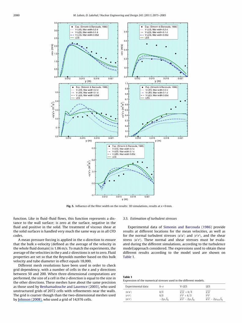

2080 M. Labois, D. Lakehal / Nuclear Engineering and Design 241 (2011) 2075–2085

e resu

ftfltc

ttapv

gbptauTb

different results according to the model used are shown onTable 1.

Table 1Expression of the numerical stresses used in the different models.

Fig. 5. Influence of the filter width on th

unction. Like in fluid–fluid flows, this function represents a dis-ance to the wall surface; is zero at the surface, negative in theuid and positive in the solid. The treatment of viscous shear athe solid surfaces is handled very much the same way as in all CFDodes.

A mean pressure forcing is applied in the x-direction to ensurehat the bulk x-velocity (defined as the average of the velocity inhe whole fluid domain) is 1.06 m/s. To match the experiments, theverage of the velocities in the y and z-directions is set to zero. Fluidroperties are set so that the Reynolds number based on this bulkelocity and tube diameter in effect equals 18,000.

Different mesh resolutions have been used in order to checkrid dependency, with a number of cells in the x and y directionsetween 50 and 200. When three-dimensional computations areerformed, the size of a cell in the z-direction is equal to the size in

he other directions. These meshes have about the same precisions those used by Benhamadouche and Laurence (2003), who usednstructured grids of 2072 cells with refinements near the walls.he grid is coarser though than the two-dimensional meshes usedy Johnson (2008), who used a grid of 14,976 cells.

lts: 3D simulations, results at x = 0 mm.

3.5. Estimation of turbulent stresses

Experimental data of Simonin and Barcouda (1986) provideresults at different locations for the mean velocities, as well asfor the normal turbulent stresses 〈u′u′〉 and 〈v′v′〉, and the shearstress 〈u′v′〉. These normal and shear stresses must be evalu-ated during the different simulations, according to the turbulencemodel/approach considered. The expressions used to obtain these

Experimental data k–ε V-LES LES

〈u′u′〉 k/3 u′u′ + k/3 u′u′

〈v′v′〉 k/3 v′v′ + k/3 v′v′

〈u′v′〉 −2�tSij u′v′ − 2�tSij u′v′ − 2�SGSSij

M. Labois, D. Lakehal / Nuclear Engineering and Design 241 (2011) 2075–2085 2081

in the

4

4

pruaaan

Lmezlt

Fig. 6. Influence of the size of the computational domain

. Results and discussion

.1. 2D simulations

Two-dimensional simulations using V-LES have first beenerformed on meshes consisting of 100 × 100 and 200 × 200,espectively (see Fig. 1). The flow was established at t = 0.3 s whennsteady turbulent structures start to appear. Results are time-veraged between t = 0.4 s and t = 0.8 s. Results of the two grids forfilter width of 0.2d are shown in Fig. 2. The comparison shows

ctually that the 100 × 100 grid may be sufficient for this Reynoldsumber. In the following, only results from this mesh will be shown.

Fig. 3 presents numerical results obtained with RANS and V-ES using different filter widths. If the mean velocities seem to

atch qualitatively the experiments, with an unsteady flow being

stablished, it can be noticed that in all cases, the recirculationone is larger than the experiments and previous reported simu-ations. This means that 2D simulations are probably not sufficiento resolve the flow.

spanwise direction: 3D simulations, results at x = 0 mm.

When looking at the results – though quantitatively – it can beseen that the Reynolds stresses are under-estimated in the vicin-ity of the walls using RANS and V-LES using various filter widths,which, both could be treated in 2D in contrast to LES. In the cen-tral part of the flow, the present results match the experiments,except in the wake of the cylinder where a larger recirculationzone is noticed. The results depart from experiments and previ-ous simulations when considering now the turbulent fluctuatingquantities. Even if the qualitative behaviour of 〈u′u′〉 and 〈v′v′〉is closer to the experimental results, the magnitude differs byat least 50%. Results of 〈u′v′〉 are far from the experiment, evenqualitatively. It seems that two-dimensional simulations fail topredict the flow near the walls, and that three-dimensional sim-ulations are necessary to capture the full effect of unsteadiness,

especially the spanwise unsteadiness. In the above result, we havealso noticed that the effect of varying the filter width on the V-LESresults could be important. This has led to us to make a system-atic sensitivity analysis of this parameter, but in 3D, as discussednext.

2082 M. Labois, D. Lakehal / Nuclear Engineering and Design 241 (2011) 2075–2085

n a m

4

bmcmffi

itRcoboflcc

Fig. 7. Comparison of LES and V-LES o

.2. 3D simulations

Three-dimensional simulations are reported in this section, foroth V-LES and LES, using the same grid. First, the influence of theesh size is analyzed, for grids of 50 × 50 × 20 and 100 × 100 × 43

ells, with a size of one diameter in the spanwise direction. Theseeshes are understandably coarse for LES, but cannot be refined

urther because of the computational costs it implies. In V-LES, thelter width is fixed to 0.1d.

As can be seen in Fig. 4, the size of the mesh has a littlenfluence only on the mean velocities 〈u〉 and 〈v〉. In contrast,he results seem to be very different when looking at theeynolds stresses. It is therefore advised to use a mesh withell width equal or less than 4.5 10−5 m. However, this thresh-ld will not be always respected in the following computations,

ecause of the computational cost involved with such a res-lution. Indeed, more than 70 h are needed to simulate theow during 1 s when using LES for a mesh of 100 × 100 × 43ells, against less than 12 h when using a mesh of 50 × 50 × 20ells.

esh of depth 1.5d, results at x = 0 mm.

The influence of the filter width for V-LES is now tested, andresults are shown in Fig. 5 for a mesh consisting of 100 × 100 × 43cells. For these simulations the depth of the computational domainin the spanwise direction is one diameter. It can be seen thatthe filter width of 0.2d provides results that are actually two-dimensional, with large variations in the normal Reynolds stressin the streamwise direction. Results obtained with the filter widthof 0.1d do not match the experimental data, particularly when look-ing at the Reynolds stresses. This behaviour could be explained bythe too small depth of our computational domain, which preventslarge spanwise structures to develop. A filter width of 0.05d, whichwould allow the smaller turbulent structures to develop, providesindeed results matching the data and LES.

To confirm this explanation, simulations with different sizes ofthe computational domain in the spanwise direction have been

conducted, with a filter width of 0.1d, and a constant cell size in alldirections of 9 × 10−4 mm. Results of this analysis are presented inFig. 6. It is clear that a depth of only 0.5d prevents three-dimensionalstructures from developing as was to be expected, and thus, theresults are the same as in the two-dimensional simulations. Using

M. Labois, D. Lakehal / Nuclear Engineering and Design 241 (2011) 2075–2085 2083

F .05d) a

aaObIdl

5c

5

tcsctbs(

i0mutisti

i

ig. 8. Comparison between experiments, TransAT LES, V-LES (with filter width = 0

depth of 1d provides better results, but this is still not sufficient,s can be observed when looking at the results for the shear stress.n the other hand, a depth of 1.5d is large enough such that the tur-ulent structures can develop, and are similar to 2d domain depth.

t is therefore recommended to use a depth of the computationalomain of at least 1.5d, or larger than 10 times the filter width, at

east.

. Validation against experiments and previousalculations

.1. Mean velocities and Reynolds stresses

Once the influences of the different computational parame-ers have been assessed, the V-LES and LES simulations are nowompared against the experimental data. Because the previous sen-itivity analysis has shown that the depth of the domain may beritical for the solution, and was subsequently increased to 1.5d,he grid resolution in the third direction was therefore increasedy factor of 15%. Note that this final mesh resolution has about theame precision as the one used by Benhamadouche and Laurence2003), albeit with only 20 cells in the spanwise direction.

The results of these final larger-depth simulations are presentedn Fig. 7, where two filter-widths have been used, namely 0.05d and.1d. Smaller filter-width results 0.05d provide very good agree-ent with both the present LES results and experiments. Results

sing a larger filter width of 0.1d deviate slightly from the data, buthey still match the measurements when looking at the mean veloc-ties in particular. Both the streamwise normal Reynolds stress and

hear stress are remarkably well predicted by V-LES as comparedo LES, although the effect of varying the filter width for this depths noticeable for the cross-flow normal stress mainly.

Comparing now the work with previous other CFD-based find-ngs using high-order turbulence models and LES, the present

nd UMIST LES and RSM. 3D simulations in all cases; results presented at x = 0.

results are overall very satisfactory. The current results slightlyunderestimate the streamwise velocity close to the walls as com-pared to Benhamadouche and Laurence (2003) and Johnson (2008)– though performed in 2D; in both these references, this quan-tity is rather slightly overestimated, while in contrast Hassan andBarsamian (2004) report very good results in this zone. Our resultsmay be explained by the fact that we do not have cell refine-ment near the walls. The current prediction for 〈v〉 is howeververy good and match that of Benhamadouche and Laurence, andare better that Johnson’s (2008) 2D results. The normal stress〈u′u′〉 is very well predicted, too, though with departures frommeasurements with about 10%. The behaviour is better than inBenhamadouche and Laurence (2003) paper, which report a largerpeak near the walls. 〈v′v′〉 is also well reproduced by our V-LES,although being slightly under-estimated in the core-flow region.The same behaviour is reported by Johnson, in contrast to Ben-hamadouche and Laurence, Hassan and Barsamian who obtainedresults with close match to the experiment. Finally, though theshear stress shows a good behaviour overall, the quantity is over-estimated near the wall and shows a shift of the peak; the samebeing reported in the LES results of Benhamadouche and Laurence.Hassan and Barsamian report instead a closer match to the experi-ment.

5.2. Direct comparison with other LES and RSM data

In order to assess the quality of the present LES simulations,our data are compared with those obtained by Benhamadoucheand Laurence (2003), using a BFC grid. The comparison is pre-

sented in Fig. 8, in which we have added the results of their RSMsimulation and our V-LES results. The RSM approach is supposedto yield better results than any RANS model, be it linear or non-linear. The argument of commercial codes being used does nothold here, since the code used by UMIST is an in-house code,

2084 M. Labois, D. Lakehal / Nuclear Engineering and Design 241 (2011) 2075–2085

-LES (

vfibs

Fig. 9. Flow structures in LES (left) and V

alidated over hundreds of test cases. The comparison showsrst that our LES are way better than their LES, part may be aetter behaviour of their model for the 〈v〉 velocity. Second, iteems that their RSM simulations provide indeed the right trend

Fig. 10. Instantaneous vorticity field. Compari

right). Fluctuating velocities u′ , v′ and w′ .

as compared to experiments, way better than our simple RANSmodel simulations (see Fig. 3), but the quality is not as good asthe present V-LES results. V-LES is clearly superior to any RANSapproach, and could even outperform is a more sophisticated sta-

son between LES (left) and V-LES (right).

eering

tE

5

hTct(iieasawftioflnmd

6

fltcomttpctisciemairasrei

Smith, L.M., Woodruff, S.L., 1998. Renormalization-group analyzes of turbulence.

M. Labois, D. Lakehal / Nuclear Engin

istical model is used in combination with LES, e.g. the RSM orASM.

.3. 3D structures of the flow

The turbulent structures of the flow are now are shown in Fig. 9,ighlighted by iso-values of the fluctuation velocities u′, v′ and w′.he figure compares LES and V-LES for a filter width of 0.1d. Itan be seen that the V-LES (right panels) reproduces indeed thehree-dimensional structures, but they are not as fine as in the LESleft panels). The difference in the size and shape of the structuress further illustrated by reporting iso-values of the total vorticityn Fig. 10. This difference in the size of the turbulent structuresxplains the different conclusions drawn between the present worknd that of Rollet-Miet et al. (1999) – also based on 3D LES – on theize of the domain in the spanwise direction: they found indeed thatdepth of one diameter was sufficient for their LES simulations,hereas a depth of at least 1.5 diameter is shown to be needed

or both the V-LES and LES to capture the three-dimensional struc-ures. The present result suggests that the large scales are the mostmportant contribution to turbulent kinetic energy, which makesf the V-LES a very good alternative to LES, at least for this class ofow. The benefit of the V-LES is mainly in reducing the CPU timeeeded for full 3D LES. The fining points out to the fact that SGSodels of various sophistication will not necessarily bring a marked

ifference compared with a simple models.

. Conclusions

In this study V-LES and LES approaches have been applied for aow across a tube bundle. The first conclusion to be drawn is thathe flow must be resolved in three-dimensions, under transientonditions, with refined grids, in line with previous CFD studiesn this subject. Indeed, three-dimensional structures, which play aajor role when evaluating the Reynolds stresses, cannot arise in

wo-dimensional simulations. Very Large Eddy Simulation has beenested, validated, and thoroughly assessed by varying various com-utational parameters: grid, filter width, domain size, and inflowonditions. This model or rather modelling approach is provedo provide the flow unsteadiness in three-dimensions, while sav-ng computational cost compared to Large Eddy Simulation. Theimulation results obtained with V-LES are very satisfactory whenompared with the data and available calculation results from var-ous other sources. As expected, the method is computationallyfficient (it can be applied using an implicit solver which per-its a higher CFL than with LES; typically CFL ∼ 1 against ∼0.1),

nd numerically robust. The computational cost decreases withncreasing filter width, though at the expenses of the quality of theesults. The RSM simulations of this flow provide the right trend

s compared to experiments, way better than simple RANS modelimulations, but the quality is not as good as the present V-LESesults. V-LES is clearly superior to any RANS approach, and couldven outperform if a more sophisticated statistical model is usedn combination with LES, e.g. the RSM or EASM. Another advantage

and Design 241 (2011) 2075–2085 2085

of the model as shown here is that it could be degenerated to a DESto better treat high-lift aerodynamics flows.

In the light of this systematic assessment investigation, V-LESseems to be a good compromise between efficiency and pre-cision, and thus may be used for industrial applications underhigh-to-very-high Reynolds number, where LES will always remainexpensive (to obtain statistically convergent results). Not limited toturbulent single phase flows only, V-LES has been recently shown tobe extendible to multiphase flow systems, including steam–watersystems such as pressurized thermal shocks and gas–liquid strati-fied flows in pipes and ducts (Lakehal and Labois, 2011).

Acknowledgements

The work was conducted using the TransAT code of ASCOMPwithin NURISP; an EC-funded project in the framework of the 7thEURATOM Framework Program. The authors are grateful to Prof. D.Laurence (UMIST) for having shared his data with us.

References

ASCOMP GmbH, 2009. Multi-Fluid Navier-Stokes Solver TransAT User Manual.Benhamadouche, S., Laurence, D., 2003. LES Coarse LES, and Transient RANS com-

parison on the flow across a tube bundle. International Journal of Heat and FluidFlow 24, 470–479.

Hassan, Y.A., Barsamian, H.R., 2004. Tube bundle flows with the large eddy simu-lation technique in curvilinear coordinates. International Journal of Heat andMass Transfer 47, 3057–3071.

Johansen, S.T., Wu, J., Shyy, W., 2004. Filtered-based unsteady RANS computations.International Journal of Heat and Fluid Flow 25, 10–21.

Johnson, R.W., 2008. Modeling strategies for unsteady turbulent flows in the lowerplenum of the VHTR. Nuclear Engineering and Design 238, 482–491.

Lakehal, D., Thiele, F., 2001. Sensitivity of turbulent shedding flows to non-linearstress–strain relations and Reynolds stress models. Computers and Fluids 30,1–35.

Lakehal, D., Labois, M. A New modeling strategy for phase-change heat trans-fer in turbulent interfacial two-phase flow. IJMF, (available online) 2011,doi:10.1016/j.ijmultiphaseflow.2011.03.004.

Launder, B.E., Spalding, D.B., 1974. The numerical computation of turbulent flows.Computer Methods in Applied Mechanics and Engineering 3, 269–289.

Moulinec, C., Pourquié, M.J.B., Boersma, B.J., Buchal, T., Nieuwstadt, F.T.M., 2004.Direct numerical simulation on a Cartesian mesh of the flow through a tubebundle. International Journal of Computational Fluid Dynamics 18 (1), 1–14.

Nicoud, F., Ducros, F., 1999. Subgrid-scale stress modelling based on the square ofthe velocity gradient tensor. Flow, Turbulence and Combustion 62, 183–200.

Norris, L.H., Reynolds, W.C., 1975. Turbulent Channel Flow with a Moving WavyBoundary, Rept. No. FM-10, Stanford University, Dept. Mech. Eng.

Peskin, C.S., 1972. Flow patterns around heart valves – numerical method. Journalof Computational Physics 10 (2), 252–271.

Rollet-Miet, P., Laurence, D., Ferziger, J., 1999. LES and RANS of turbulent flow intube bundles. International Journal of Heat and Fluid Flow 20, 241–254.

Ruprecht, A., Helnrich, T., Buntic, I., 2003. Very Large Eddy Simulation for the pre-diction of unsteady cortex motion. In: Symposium of the 12th InternationalConference on Fluid Flow Technology , Budapest, Hungary.

Simonin, O., Barcouda, M., 1986. Measurements of fully developed turbulent flowacross tube bundle. In: Third International Symposium on Applications of LaserAnemometry to Fluid Mechanics , Lisbon, Portugal, pp. 21.5.1–21.5.5.

Annual Review of Fluid Mechanics 30, 275–310.Spalart, P.R., Allmaras, S.R., 1992. A One-Equation Turbulence Model for Aerody-

namic Flows, AIAA Paper 92-0439.Speziale, C.G., 1998. Turbulence modelling for time-dependent RANS and VLES: a

review. AIAA Journal 36 (2), 173–184.