
A new hybrid method using evolutionary algorithms to train Fuzzy Cognitive Maps
23
A new hybrid method using evolutionary algorithms to train Fuzzy Cognitive Maps Elpiniki I. Papageorgiou * , Peter P. Groumpos Department of Electrical and Computer Engineering, Laboratory for Automation and Robotics, Artificial Intelligence Research Center (UPAIRC), University of Patras, Rion 26500, Greece Received 1 September 2003; received in revised form 2 August 2004; accepted 5 August 2004 Abstract A novel hybrid method based on evolutionary computation techniques is presented in this paper for training Fuzzy Cognitive Maps. Fuzzy Cognitive Maps is a soft computing technique for modeling complex systems, which combines the synergistic theories of neural networks and fuzzy logic. The methodology of developing Fuzzy Cognitive Maps relies on human expert experience and knowledge, but still exhibits weaknesses in utilization of learning methods and algorithmic background. For this purpose, we investigate a coupling of differential evolution algorithm and unsupervised Hebbian learning algorithm, using both the global search capabilities of Evolutionary strategies and the effectiveness of the nonlinear Hebbian learning rule. The use of differential evolution algorithm is related to the concept of evolution of a number of individuals from generation to generation and that of nonlinear Hebbian rule to the concept of adaptation to the environment by learning. The hybrid algorithm is introduced, presented and applied successfully in real-world problems, from chemical industry and medicine. Experimental results suggest that the hybrid strategy is capable to train FCM effectively leading the system to desired states and determining an appropriate weight matrix for each specific problem. # 2004 Elsevier B.V. All rights reserved. Keywords: Fuzzy Cognitive Maps; Learning algorithms; Nonlinear Hebbian rule; Evolutionary computation; Differential evolution algorithms; Evolutionary training 1. Introduction Fuzzy Cognitive Maps (FCMs) were proposed by Kosko to represent the causal relationship between concepts and analyze inference patterns [23,24]. FCMs represent knowledge in a symbolic manner and relate states, processes, events, values and inputs in an analogous manner. Compared either expert system or neural networks, it has several desirable properties, such as it is relatively easy to use for representing structured knowledge, and the inference can be computed by numeric matrix operation. FCMs are appropriate to explicit the knowledge which has www.elsevier.com/locate/asoc Applied Soft Computing 5 (2005) 409–431 * Corresponding author. Tel.: +30 2610997293; fax: +30 26120997309. E-mail addresses: [email protected] (E.I. Papageorgiou), [email protected] (P.P. Groumpos). 1568-4946/$ – see front matter # 2004 Elsevier B.V. All rights reserved. doi:10.1016/j.asoc.2004.08.008
Transcript of A new hybrid method using evolutionary algorithms to train Fuzzy Cognitive Maps
www.elsevier.com/locate/asoc
Applied Soft Computing 5 (2005) 409–431
A new hybrid method using evolutionary algorithms
to train Fuzzy Cognitive Maps
Elpiniki I. Papageorgiou*, Peter P. Groumpos
Department of Electrical and Computer Engineering, Laboratory for Automation and Robotics,
Artificial Intelligence Research Center (UPAIRC), University of Patras, Rion 26500, Greece
Received 1 September 2003; received in revised form 2 August 2004; accepted 5 August 2004
Abstract
A novel hybrid method based on evolutionary computation techniques is presented in this paper for training Fuzzy Cognitive
Maps. Fuzzy Cognitive Maps is a soft computing technique for modeling complex systems, which combines the synergistic
theories of neural networks and fuzzy logic. The methodology of developing Fuzzy Cognitive Maps relies on human expert
experience and knowledge, but still exhibits weaknesses in utilization of learning methods and algorithmic background. For this
purpose, we investigate a coupling of differential evolution algorithm and unsupervised Hebbian learning algorithm, using both
the global search capabilities of Evolutionary strategies and the effectiveness of the nonlinear Hebbian learning rule. The use of
differential evolution algorithm is related to the concept of evolution of a number of individuals from generation to generation
and that of nonlinear Hebbian rule to the concept of adaptation to the environment by learning. The hybrid algorithm is
introduced, presented and applied successfully in real-world problems, from chemical industry and medicine. Experimental
results suggest that the hybrid strategy is capable to train FCM effectively leading the system to desired states and determining an
appropriate weight matrix for each specific problem.
# 2004 Elsevier B.V. All rights reserved.
Keywords: Fuzzy Cognitive Maps; Learning algorithms; Nonlinear Hebbian rule; Evolutionary computation; Differential evolution
algorithms; Evolutionary training
1. Introduction
Fuzzy Cognitive Maps (FCMs) were proposed by
Kosko to represent the causal relationship between
* Corresponding author. Tel.: +30 2610997293;
fax: +30 26120997309.
E-mail addresses: [email protected]
(E.I. Papageorgiou), [email protected] (P.P. Groumpos).
1568-4946/$ – see front matter # 2004 Elsevier B.V. All rights reserved
doi:10.1016/j.asoc.2004.08.008
concepts and analyze inference patterns [23,24].
FCMs represent knowledge in a symbolic manner
and relate states, processes, events, values and inputs
in an analogous manner. Compared either expert
system or neural networks, it has several desirable
properties, such as it is relatively easy to use for
representing structured knowledge, and the inference
can be computed by numeric matrix operation. FCMs
are appropriate to explicit the knowledge which has
.
E.I. Papageorgiou, P.P. Groumpos / Applied Soft Computing 5 (2005) 409–431410
been accumulated for years on the operation of a
complex system.
In recent years, there is an increase of published
journals and conference papers on FCMs. FCMs have
already been applied in many scientific areas, such as
medicine, manufacturing, organization behaviour,
political science, industry [3,10,22,27,30,34,35,39,
40,48,49,55].
This research work proposes a hybrid FCM
learning procedure based on the combination of an
unsupervised learning rule, the nonlinear Hebbian
learning (NHL) rule and an evolutionary computation
(EC)-based algorithm, the differential evolution, to
improve the FCM structure, to eliminate the defi-
ciencies in the usage of FCMs and to enhance the
dynamical behavior and flexibility of the FCM model.
Very few research efforts have been made till today to
propose an appropriate learning algorithm suitable for
FCMs [1,24,33,36–38].
Artificial neural networks and evolutionary compu-
tation establish two major research and application
areas in artificial intelligence. In analogy to biological
neural networks, artificial neural networks (ANNs) are
composed of simple processing elements that interact
using weighted interconnections and are of particular
interest because of their robustness, their parallelism,
and their learning abilities [14,15]. Evolutionary
computation is typically considered in the context of
evolutionary algorithms (EAs). Evolutionary algo-
rithms are a very rich class of multi-agent stochastic
search algorithms based on the neo-Darwinian para-
digm of natural evolution, which can perform
exhaustive searches in complex solution spaces. These
techniques start with searching a population of feasible
solutions generated stochastically. Then, stochastic
variations are incorporating into the parameters of the
population in order to evolve the solution to a global
optimum [12,18]. EAs establish a very general and
powerful search, optimization and learning method that
bases, in analogy to biological evolution, on the
application of evolutionary operators like mutation,
recombination and selection. Like no other computa-
tional method, EAs have been applied to a very broad
range of problems [2,4,28,43, 44,45,47].
Recently, the idea of combining ANNs and EAs has
received much attention [7,11,51], and now there is a
large body of literature on this subject. Weiss [52] in
his research work, provides a comprehensive and
compact overview of hybrid work done in artificial
intelligence, and shows the state of the art of
combining artificial neural networks and evolutionary
algorithms. There are two ways of synthesizing the
fields of ANNs and EAs; one way is to use EAs instead
of standard neural learning algorithms for training
ANNs; see e.g. [7], and the other way deals with the
approaches to an ‘‘evolution-based’’ design of appro-
priate structures of ANNs [17,42]. Furthermore, other
hybrid evolutionary approaches have been proposed
recently [25,29,52,53,54].
In this work, we use the differential evolution (DE)
algorithms, which can be easily implemented and they
are computationally inexpensive, since their memory
and CPU speed requirements are low [41]. Moreover,
they do not require gradient information of the
objective function under consideration, but only its
values, and they use only primitive mathematical
operators. DE algorithms can also handle nondiffer-
entiable, nonlinear and multimodal objective func-
tions efficiently, and require few easily chosen control
parameters. Experimental results have shown that DE
algorithms have good convergence properties and
outperform other evolutionary algorithms [46,47].
This paper proposes a new hybrid evolutionary
algorithm (HEA) for FCM learning. The HEA could
conceptually be split-up into two stages. In the first
stage, nonlinear Hebbian learning is adopted using a
recently proposed approach [36]. In the second stage,
a differential evolution (DE) algorithm, [47], is used
for FCM retraining. The usage of DE algorithm is
based on the assumption that the first stage has
produced a ‘‘good’’ solution that can be incorporated
directly into the genes and inherited by offspring. By
this manner, the initial expert knowledge (a priori),
incorporated in FCMs, can be extracted and incorpo-
rated in evolutionary computation, initializing the DE
population.
It is used in two termination conditions for the
nonlinear Hebbian learning algorithm on the first stage
of the proposed learning process and a fitness function
appropriate for the specific problem in the second
stage of the algorithm. If the optimization criterion
(minimization of fitness function) is reached in the
second stage, the algorithmic process has terminated.
This two-stage learning algorithm is used to train three
different FCM models with increasing complexity,
two FCM models for chemical process control
E.I. Papageorgiou, P.P. Groumpos / Applied Soft Computing 5 (2005) 409–431 411
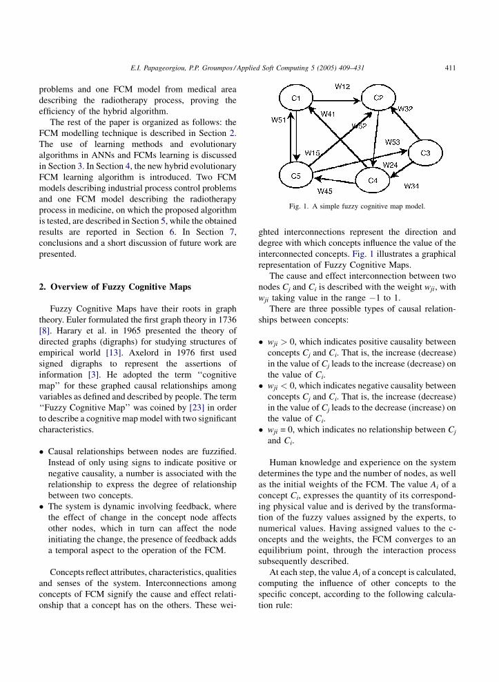
Fig. 1. A simple fuzzy cognitive map model.
problems and one FCM model from medical area
describing the radiotherapy process, proving the
efficiency of the hybrid algorithm.
The rest of the paper is organized as follows: the
FCM modelling technique is described in Section 2.
The use of learning methods and evolutionary
algorithms in ANNs and FCMs learning is discussed
in Section 3. In Section 4, the new hybrid evolutionary
FCM learning algorithm is introduced. Two FCM
models describing industrial process control problems
and one FCM model describing the radiotherapy
process in medicine, on which the proposed algorithm
is tested, are described in Section 5, while the obtained
results are reported in Section 6. In Section 7,
conclusions and a short discussion of future work are
presented.
2. Overview of Fuzzy Cognitive Maps
Fuzzy Cognitive Maps have their roots in graph
theory. Euler formulated the first graph theory in 1736
[8]. Harary et al. in 1965 presented the theory of
directed graphs (digraphs) for studying structures of
empirical world [13]. Axelord in 1976 first used
signed digraphs to represent the assertions of
information [3]. He adopted the term ‘‘cognitive
map’’ for these graphed causal relationships among
variables as defined and described by people. The term
‘‘Fuzzy Cognitive Map’’ was coined by [23] in order
to describe a cognitive map model with two significant
characteristics.
� C
ausal relationships between nodes are fuzzified.Instead of only using signs to indicate positive or
negative causality, a number is associated with the
relationship to express the degree of relationship
between two concepts.
� T
he system is dynamic involving feedback, wherethe effect of change in the concept node affects
other nodes, which in turn can affect the node
initiating the change, the presence of feedback adds
a temporal aspect to the operation of the FCM.
Concepts reflect attributes, characteristics, qualities
and senses of the system. Interconnections among
concepts of FCM signify the cause and effect relati-
onship that a concept has on the others. These wei-
ghted interconnections represent the direction and
degree with which concepts influence the value of the
interconnected concepts. Fig. 1 illustrates a graphical
representation of Fuzzy Cognitive Maps.
The cause and effect interconnection between two
nodes Cj and Ci is described with the weight wji, with
wji taking value in the range �1 to 1.
There are three possible types of causal relation-
ships between concepts:
� w
ji > 0, which indicates positive causality betweenconcepts Cj and Ci. That is, the increase (decrease)
in the value of Cj leads to the increase (decrease) on
the value of Ci.
� w
ji < 0, which indicates negative causality betweenconcepts Cj and Ci. That is, the increase (decrease)
in the value of Cj leads to the decrease (increase) on
the value of Ci.
� w
ji = 0, which indicates no relationship between Cjand Ci.
Human knowledge and experience on the system
determines the type and the number of nodes, as well
as the initial weights of the FCM. The value Ai of a
concept Ci, expresses the quantity of its correspond-
ing physical value and is derived by the transforma-
tion of the fuzzy values assigned by the experts, to
numerical values. Having assigned values to the c-
oncepts and the weights, the FCM converges to an
equilibrium point, through the interaction process
subsequently described.
At each step, the value Ai of a concept is calculated,
computing the influence of other concepts to the
specific concept, according to the following calcula-
tion rule:
E.I. Papageorgiou, P.P. Groumpos / Applied Soft Computing 5 (2005) 409–431412
Aðkþ1Þi ¼ f A
ðkÞi þ
XN
j 6¼ ij¼1
AðkÞj � wji
0BBB@
1CCCA (1)
where Aðkþ1Þi is the value of concept Ci at simulation
step k + 1, AðkÞj is the value of concept Cj at simulation
step k, wji is the weight of the interconnection between
concept Cj and concept Ci and f is the sigmoid thresh-
old function:
f ¼ 1
1 þ e�lx(2)
where l > 0, is a parameter that determines its steep-
ness. In our approach, the value l = 1 has been used.
This function is selected since the values Ai of the
concepts, must lie within [0, 1]. The interaction of the
FCM results after a few iterations in a steady state, i.e.
the values of the concepts are not modified further.
Desired values of the output concepts of the FCM
guarantee the proper operation of the simulated
system.
The methodology for developing FCMs is based on
a group of experts who are asked to define concepts
and describe relationships among concepts and use
IF–THEN rules to justify the cause and effect
relationship among concepts and infer a linguistic
weight for each interconnection [49,50]. Every expert
describes each one of the interconnection with a fuzzy
rule; the inference of the rule is a linguistic variable,
which describes the relationship between the two
concepts according to everyone expert and determines
the grade of causality between the two concepts. Then,
the inferred linguistic weights suggested by the group
of experts are composed and an overall linguistic
weight is produced through the SUM technique
[21,26]. Finally, the Center of Area (CoA) defuzzi-
fication method [21], is used for the transformation of
the linguistic weight to a numerical value of weight
wji, belonging to the interval [�1, 1] and representing
the overall suggestion of experts. This methodology
has the advantage that experts are not required to
assign directly numerical values to causality relation-
ships, but rather to describe qualitatively the degree of
causality among the concepts. Thus an initial weight
matrix Winitial =[wji], i,j = 1, . . ., N, with wii = 0, i = 1,
.., N, is obtained. Using the initial concept values, Ai,
the matrix Winitial is used for the determination of the
steady state of the FCM, through the application of Eq.
(1).
The most significant weaknesses of the FCMs are
their dependence on the experts’ opinion and the
potential uncontrollable convergence to undesired
states. The desired steady state is characterized by
values of the FCM output concepts accepted by the
experts, ex post. A novel learning procedure that
alleviates the problem of the potential convergence to
an undesired state for the output concepts values and
incorporating the knowledge in evolutionary com-
putation is proposed in this paper. This approach is
based on a hybrid method using differential evolution
algorithms and unsupervised learning algorithms,
and is described extensively in the Section 4. Also,
through the learning procedure, the optimum
available set of weights of each FCM model is
derived.
3. Learning algorithms in artificial neural
networks
Generally, in artificial neural networks (ANNs), the
weight–learning rule requires the definition and
calculation of an objective function (usually an error
function) examining when the objective function
reaches a minimum error that corresponds to a set of
weights of ANN. When the objective function is zero
or conveniently small; then, a steady state for the ANN
is reached; the weights of ANN that correspond to
steady-state define the learning process and the ANN
model [14,56].
The selection of the objective function and the
optimization method is crucial since it may promote
stability, instability, or a solution trapped in a local
minimum. Usually, during learning process, the
objective function decreases or increases, depending
on the specific assumptions of the problem, and the
weights are updated. The decrease may be accom-
plished with different optimization techniques, includ-
ing the Delta Rule, gradient-descent methods,
Boltzman’s algorithm, the back-propagation learning
algorithm, simulated annealing, and evolutionary
computation. Unsupervised Hebbian learning is
designed to maximize the variance of the output of
a given unit, and reinforcement learning is designed to
maximize the average reinforcement signal [14,26].
E.I. Papageorgiou, P.P. Groumpos / Applied Soft Computing 5 (2005) 409–431 413
Many attempts have been made within the artificial
intelligence community to integrate ANNs and
evolutionary algorithms (EAs). A number of attempts
have concentrated on applying evolutionary principles
to improve the generalization of ANNs, discover the
appropriate network topology, and the best available
set of weights [7,11,52]. The majority of approaches in
which evolutionary principles are used in conjunction
with ANN training formulates the problem of finding
the weights of a fixed neural architecture, when the
whole set of examples is available, as an optimization
problem.
Evolutionary algorithms differ substantially from
more traditional search and optimization methods.
The most significant differences are: (a) EAs search a
population of points in parallel, not a single point, (b)
They do not require derivative information or other
auxiliary knowledge; only the objective function and
corresponding fitness levels influence the directions of
search, (c) they use probabilistic transition rules, not
deterministic ones, (d) they are generally more
straightforward to apply and (e) they can provide a
number of potential solutions to a given problem. The
final choice is left to the user [5,6].
Here, we use the differential evolution (DE)
algorithms, which have been designed as stochastic
parallel direct search methods that can handle
nondifferentiable, nonlinear and multi-modal objec-
tive functions efficiently and require few easily chosen
control parameters [46,47]. Storn and Price [47] has
reported impressive results that show DE outper-
formed other evolutionary methods and the stochastic
differential equations approach on solving some
benchmark continuous parameter optimization pro-
blems.
3.1. Description of the differential evolution
algorithm
The DE algorithm, which has been developed by
Storn and Price [47], utilizes N, n-dimensional
parameter weight vectors wi;G i = 1, . . ., N, as a
population for each iteration, called generation, of the
algorithm. The initial population is taken to be
uniformly distributed in the search space. At each
iteration, the mutation and crossover operators are
applied on the individuals, and a new population
arises. Then, the selection phase starts, where the N
best points from both populations are selected to
comprise the next generation.
According to the mutation operator, for each
weight vector, wi;G, i = 1, . . ., N, a mutant vector is
determined through the equation:
vi;Gþ1 ¼ wr1;G þ mðwr2;G � wr3;GÞ (3)
where r1, r2, r3 2 {1, . . ., N}, are mutually different
random indexes and also different from the current
index, i. m 2 (0, 2] is a real constant parameter that
affects the differential variation between two vectors,
and N must be greater than or equal to 4, in order to
apply mutation. Following the mutation phase, the
crossover operator is applied on the population, com-
bining the previously mutated vector,
vi;Gþ1 ¼ ½v1i;Gþ1; v2i;Gþ1; . . . ; vDi;Gþ1� (4)
with a so-called target vector,
wi;Gþ1 ¼ ½w1i;Gþ1;w2i;Gþ1; . . . ;wDi;Gþ1� (5)
Thus a so-called trial vector,
ui;Gþ1 ¼ ½u1i;Gþ1; u2i;Gþ1; . . . ; uDi;Gþ1� (6)
is generated, according to:
uji;Gþ1 ¼ vji;Gþ1; if ðrandbðjÞ � CRÞ or j ¼ rnbrðiÞ(7)
or
uji;Gþ1 ¼ wji;G; if ðrandbðjÞ>CRÞ or j 6¼ rnbrðjÞ (8)
where i = l, . . ., N, randb(j) 2 [0, 1] is the jth evalua-
tion of a uniform random number generator, for j 2 1,
2, . . ., D, and rnbr(i) 2 1, 2, . . ., d is a randomly
chosen index. CR 2 [0, 1] is the crossover constant
(user defined), a parameter that increases the diversity
of the individuals in the population. The three algo-
rithm parameters that steer the search of the algorithm
are the population size (N), the crossover constant
(CR) and the differential variation factor (m). They
remain constant during an optimization.
To decide whether or not the vector ui,G+1 should be
a member of the population comprising the next
generation, it is compared to the initial vector wi;G.
Thus,
wi;Gþ1 ¼ ui;Gþ1; f ðui;Gþ1Þ< f ðwi;GÞwi;G; otherwise
�(9)
E.I. Papageorgiou, P.P. Groumpos / Applied Soft Computing 5 (2005) 409–431414
The procedure described above is considered as the
standard variant of the DE algorithm. Different
mutation and crossover operators have been applied
with promising results [47]. In addition, DE algo-
rithms have a property that Price has called a universal
global mutation mechanism or globally correlated
mutation mechanism, which seems to be the main
property responsible for the appealing performance of
DE as global optimizers.
To apply DE algorithms to ANNs training someone
starts with a specific number (N) of n-dimensional
weight vectors, as an initial weight population, and
evolve them over time; N is fixed throughout the
training process, and the weight population is
initialized randomly following a uniform probability
distribution. At each iteration, called generation, new
weight vectors are generated by the combination of the
weight vectors randomly chosen from the population.
This operation is called mutation. The derived weight
vectors are then mixed with another predetermined
weight vector, the ‘‘target’’ vector, through the
crossover operation. This operation yields the so-
called trial vector. The trial vector is accepted for the
next generation if and only if it reduces the value of the
error function E. This last operation is called selection.
The above-mentioned operations introduce diversity
in the population and are used to help the algorithm
escape the local minima in the weight space. The
combined action of mutation and crossover is
responsible for much of the effectiveness of DE’s
search, and allows them to act as parallel, noise-
tolerant, hill-climbing algorithms, which efficiently
search the whole weight space.
3.2. Learning methods in Fuzzy Cognitive Maps
FCM learning involves updating the strengths of
causal links. Combining multiple FCMs is the
simplest form of learning. An alternative learning
strategy is to improve FCMs by fine-tuning its initial
causal link or edge strengths through training similar
to that in artificial neural networks. This way of
learning is more effective and more efficient to
accurately adjust the FCM cause–effect relationships.
Up-to-date, there are just a few FCM learning
algorithms [1,23,24,36–38] and they are mostly based
on ideas coming from the field of artificial neural
networks training. Kosko has developed the first
algorithm, named differential Hebbian learning, as a
form of unsupervised learning, but without mathe-
matical formulation and implementation in real
problems [23]. There is no guarantee that DHL will
encode the sequence into the FCM and till today no
concrete procedures exist for applying DHL in FCMs.
Another proposed algorithm is the Adaptive Random
for FCMs learning based on the theoretical aspects of
Random Neural Networks [1]. These algorithms start
from an initial state and an initial weight matrix of the
FCM and adapt the weights in order to compute a
weight matrix that leads the FCM to a desired state.
Also, recently, two unsupervised learning techni-
ques, the active Hebbian learning (AHL) and the
nonlinear Hebbian learning (NHL) algorithms, have
been proposed to fine-tune FCM causal links in order
to succeed desired values for output concepts and
acceptable operation for the system keeping its
constraints [36,37]. These algorithms were imple-
mented successfully in a practical control problem.
The AHL algorithm introduced a sequence of
activation concepts depending on the problem’s
configuration and characteristics [37]. Thus, activation
and activated concepts were bringing on. Experts
determined the mode of activation between concepts
(asynchronous or not) and the number and sequence of
activation concepts. When the AHL algorithm
terminates and the system converges in desired state
(means that the values of decision-output concepts are
accepted), a new updated weight matrix is derived,
determining new cause–effect relationships between
the concepts of FCM model, which are desired for
each case-study scenario.
Also, except the unsupervised learning-based
techniques for FCMs, methods based on evolutionary
computation techniques have been investigated.
Particle Swarm Optimization (PSO) method has been
used for first time and has been proposed for FCM
learning giving very promising results [38]. Using this
learning approach, a number of sub-optimum weight
matrices is derived leading the values of output
concepts within the desired regions and alleviating the
problem of the potential convergence to an undesired
steady state. More investigation is needed for this
method and generally for evolutionary computation
methods [38].
The present work focuses on the development of an
FCM learning procedure based on a hybrid evolu-
E.I. Papageorgiou, P.P. Groumpos / Applied Soft Computing 5 (2005) 409–431 415
tionary algorithm. The purpose is to determine the
appropriate or optimum values of the cause effect
relationships among the concepts, i.e. the optimum set
of the weights of the FCM, that produce the desired
behavior of the system. The determination of the
appropriate set of the weights is of major significance
and it contributes towards the establishment of FCMs
as a robust methodology. The desired behavior of the
system is characterized by output concept values that
lie within desired bounds prespecified by the experts.
These bounds are in general problem-dependent.
4. The hybrid evolutionary algorithm
In this section, we present the hybrid method
combined of differential evolution algorithm and
nonlinear Hebbian learning (NHL) algorithm for
FCMs. The DE algorithm works on the termination
point of NHL algorithm. Thus the method consists of a
NHL-based FCM training stage and a differential
evolutionary strategy-based FCM retraining stage.
4.1. First stage: nonlinear Hebbian learning
algorithm for FCMs
The proposed learning procedure is based on the
nonlinear Hebbian-type learning rule for ANNs
learning [36]. This unsupervised learning rule have
been adapted and modified for the FCM case,
determining the nonlinear Hebbian learning (NHL)
algorithm.
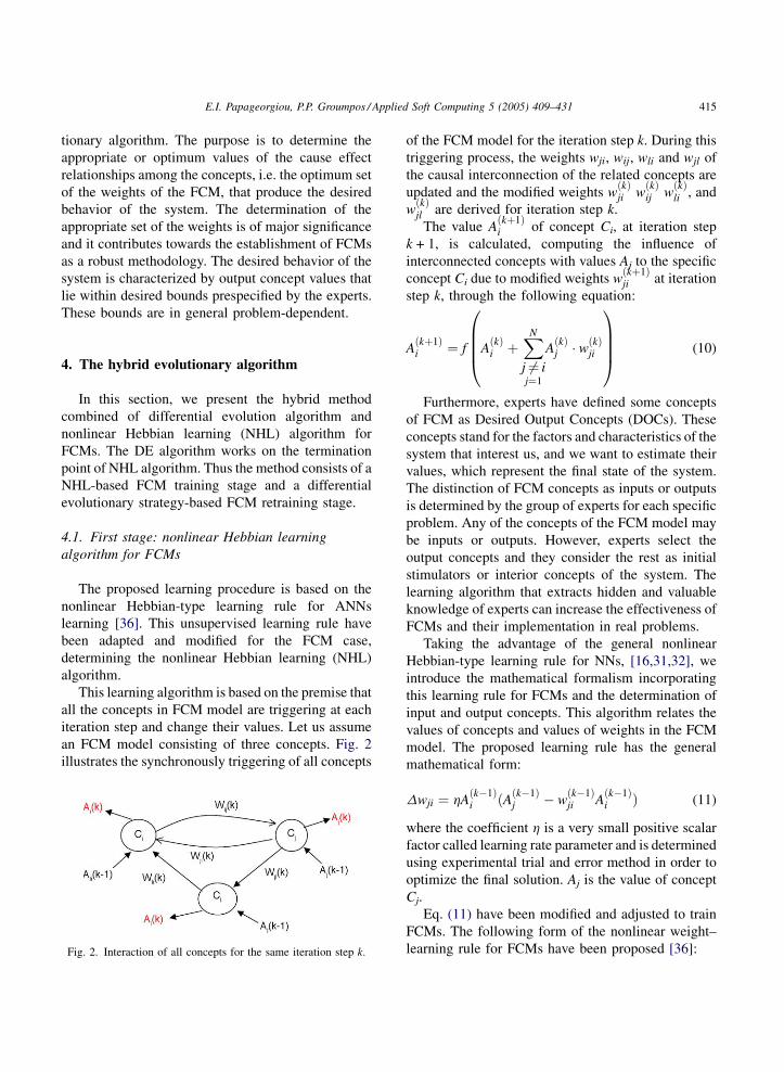
This learning algorithm is based on the premise that
all the concepts in FCM model are triggering at each
iteration step and change their values. Let us assume
an FCM model consisting of three concepts. Fig. 2
illustrates the synchronously triggering of all concepts
Fig. 2. Interaction of all concepts for the same iteration step k.
of the FCM model for the iteration step k. During this
triggering process, the weights wji, wij, wli and wjl of
the causal interconnection of the related concepts are
updated and the modified weights wðkÞji w
ðkÞij w
ðkÞli , and
wðkÞjl are derived for iteration step k.
The value Aðkþ1Þi of concept Ci, at iteration step
k + 1, is calculated, computing the influence of
interconnected concepts with values Aj to the specific
concept Ci due to modified weights wðkþ1Þji at iteration
step k, through the following equation:
Aðkþ1Þi ¼ f A
ðkÞi þ
XN
j 6¼ ij¼1
AðkÞj w
ðkÞji
0BBB@
1CCCA (10)
Furthermore, experts have defined some concepts
of FCM as Desired Output Concepts (DOCs). These
concepts stand for the factors and characteristics of the
system that interest us, and we want to estimate their
values, which represent the final state of the system.
The distinction of FCM concepts as inputs or outputs
is determined by the group of experts for each specific
problem. Any of the concepts of the FCM model may
be inputs or outputs. However, experts select the
output concepts and they consider the rest as initial
stimulators or interior concepts of the system. The
learning algorithm that extracts hidden and valuable
knowledge of experts can increase the effectiveness of
FCMs and their implementation in real problems.
Taking the advantage of the general nonlinear
Hebbian-type learning rule for NNs, [16,31,32], we
introduce the mathematical formalism incorporating
this learning rule for FCMs and the determination of
input and output concepts. This algorithm relates the
values of concepts and values of weights in the FCM
model. The proposed learning rule has the general
mathematical form:
Dwji ¼ hAðk�1Þi ðAðk�1Þ
j � wðk�1Þji A
ðk�1Þi Þ (11)
where the coefficient h is a very small positive scalar
factor called learning rate parameter and is determined
using experimental trial and error method in order to
optimize the final solution. Aj is the value of concept
Cj.
Eq. (11) have been modified and adjusted to train
FCMs. The following form of the nonlinear weight–
learning rule for FCMs have been proposed [36]:
E.I. Papageorgiou, P.P. Groumpos / Applied Soft Computing 5 (2005) 409–431416
wðkÞji ¼ g w
ðk�1Þji þ hA
ðk�1Þj ðAðk�1Þ
j
� sgn ðwjiÞwðk�1Þji A
ðk�1Þi Þ (12)
where the h is the learning rate parameter and g is the
weight decay parameter. The term sgn (wji) is used to
maintain the sign of the corresponding weight (and
further to keep the physical meaning of relationships
for the examined problem), and the term
�sgn ðwjiÞwðk�1Þji ðAk�1
i Þ2 is used to avoid potential
undesired increase on the weight values from the
initial experts knowledge. Based on the previous
equation, the values of weights are modified at a small
amount comparing with the initial weights because the
second term of Eq. (12) is small in correlation to the
first term gwðk�1Þji .
Using the NHL algorithm only, the initially
nonzero weights suggested by experts are updated
for each iteration step. The value of each concept of
FCM is updated, through the Eq. (10) where the value
of weight wðkÞji is calculated using Eq. (12). Also, we
use two termination functions for the termination of
the proposed algorithm.
The first termination function F1 have been
proposed for the NHL algorithm for examining the
accepted values of outputs concepts, which are the
values of DOCs, we are interested about [36].
The termination function F1 have been defined as:
F1 ¼ jDOCi � Tij2 (13)
where Ti is the mean target value of the interesting
concept DOCi. This type of criterion function (which
has the classic form of Euclidean distance) is appro-
priate for the NHL rule for FCMs. The minimization
of the termination function F1 is the goal, updating the
weights and determining the learning process.
Let us assume that we are interested to calculate F1
of concept Ci with value DOCi. It is supposed that
DOCi take values in the range DOCi ¼ ½Tmini ; Tmax
i �.Then, the target value Ti of the interesting concept Ci is
determined as:
Ti ¼Tmin
i þ Tmaxi
2(14)
If we consider the case of an FCM-model, where
there are m-DOCs, then, for the calculation of F1, we
take the sum of the square differences between the m-
DOCs values with the m-Ts (mean values of DOCs),
and the Eq. (13) takes the following form:
F1 ¼ffiffiffiffiffiffiffiffiffiffiffiffiffiffiffiffiffiffiffiffiffiffiffiffiffiffiffiffiffiffiffiffiffiffiXm
i¼1
ðDOCi � TiÞ2
s(15)
The second termination condition is determined by
the variation of the subsequent values of DOCi, for
iteration step k, yielding a value e, which has to be as
less as possible, taking the form:
F2 ¼ jDOCðkþ1Þi � DOC
ðkÞi j< e ¼ 0:005 (16)
where DOCi is the value of ith concept.
Through this process and when the termination
conditions are met, the final weight matrix WNHL, is
derived.
In NHL algorithm, upper and lower bounds for the
learning parameters g and h have been determined
using trial and error experiments, because we
proposed small modifications on the values of weights
according to their initial values. So, constant values for
each one are calculated for specific case-study
problem. The values of parameters h and g, for each
specific case, ensure that the learning process
converges fast in a desired state.
It was observed after a large number of simulations
for different values for parameters h and g, that using
large values for parameter h, the weights change their
values at a significant amount causing also changes on
their signs. For same simulation using small constant
values for the parameter g, the weights continue to
change their values significantly, and the FCM
concepts cannot take values within a desired region.
The bounds of learning rate parameter h have been
determined as 0 < h < 0.1, and for the weight decay
parameter have been determined as 0.9 < g < 1, after
simulation results for each case problem [36].
A generic description of the proposed hybrid
algorithm is given in Algorithm 1.
Algorithm 1 (Generic Model of the Hybrid FCM
Learning Algorithm).
Stage 1: Nonlinear Hebbian learning
Step 1a:
Read input concept state A0 andinitial weight matrix W0.
Step 2a: Repeat for each iteration k.Step 3a:
Calculate A(k) according to the Eq. (10).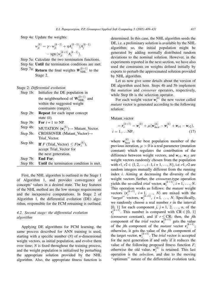
E.I. Papageorgiou, P.P. Groumpos / Applied Soft Computing 5 (2005) 409–431 417
Step 4a:
Update the weights:wðkÞji ¼ g w
ðk�1Þji þ hA
ðk�1Þi ðAðk�1Þ
j
� sgn ðwðkþ1Þji A
ðk�1Þi Þ:
Step 5a:
Calculate the two termination functions.Step 6a:
Until the termination conditions are met.Step 7a:
Return the final weights Wðkþ1ÞNHL to theStage 2.
Stage 2: Differential evolution
Step 1b:
Initialize the DE population inthe neighbourhood of Wðkþ1ÞNHL and
within the suggested weight
constraints (ranges).
Step 2b:
Repeat for each input conceptstate (k).
Step 3b:
For i = 1 to NP.Step 4b:
MUTATION (wðkÞi )! Mutant_Vector.Step 5b:
CROSSOVER (Mutant_Vector)!Trial_Vector.Step 6b:
If F (Trial_Vector) � F(wðkÞi ),accept Trial_Vector for
the next generation.
Step 7b:
End For.Step 8b:
Until the termination condition is met.First, the NHL algorithm is outlined in the Stage 1
of Algorithm 1, and provides convergence of
concepts’ values in a desired state. The key features
of the NHL method are the low storage requirements
and the inexpensive computations. In Stage 2 of
Algorithm 1, the differential evolution (DE) algo-
rithm, responsible for the FCM retraining is outlined.
4.2. Second stage: the differential evolution
algorithm
Applying DE algorithms for FCM learning, the
same process described for ANN training is used,
starting with a specific number (N) of n-dimensional
weight vectors, as initial population, and evolve them
over time; N is fixed throughout the training process,
and the weight population is initialised by perturbing
the appropriate solution provided by the NHL
algorithm. Also, the appropriate fitness function is
determined. In this case, the NHL algorithm seeds the
DE, i.e. a preliminary solution is available by the NHL
algorithm; so, the initial population might be
generated by adding normally distributed random
deviations to the nominal solution. However, in the
experiments reported in the next section, we have also
used the constraints on weights defined initially by
experts to perturb the approximated solution provided
by NHL algorithm.
Let us now give some details about the version of
DE algorithm used here. Steps 4b and 5b implement
the mutation and crossover operators, respectively,
while Step 6b is the selection operator.
For each weight vector wðkÞi the new vector called
mutant vector is generated according to the following
relation:
Mutant vector
¼ vðkþ1Þi ¼ w
ðkÞi þ mðwðkÞ
best � wðkÞi þ wr1 � wr2Þ;
i ¼ 1; . . .NP; (17)
where wðkÞbest is the best population member of the
previous iteration, m > 0 is a real parameter (mutation
constant) which regulates the contribution of the
difference between weight vectors, and wr1, wr2 are
weight vectors randomly chosen from the population
with r1, r2 2 {l, 2, . . ., i�l, i + 1, . . ., N}, i.e. r1, r2 are
random integers mutually different from the running
index i. Aiming at decreasing the diversity of the
weight vectors further, the crossover-type operation
yields the so-called trial vector, uðkþ1Þi , i = 1, . . ., N.
This operation works as follows: the mutant weight
vectors (vðkþ1Þi , i = 1, . . ., N) are mixed with the
‘‘target’’ vectors, wðkþ1Þi , i = l, . . ., N. Specifically,
we randomly choose a real number r in the interval
[0, 1] for each component j, j = 1, 2, . . ., n, of the
vðkþ1Þi . This number is compared with CR 2 [0, 1]
(crossover constant), and if r � CR; then, the jth
component of the trial vector uðkþ1Þi gets the value
of the jth component of the mutant vector vðkþ1Þi ;
otherwise, it gets the value of the jth component of
the target vector, wðkþ1Þi . The trial vector is accepted
for the next generation if and only if it reduces the
value of the following proposed fitness function F;
otherwise the old value, wðkÞi is retained. This last
operation is the selection, and due to the moving
‘‘optimum’’ nature of the differential evolution task,

E.I. Papageorgiou, P.P. Groumpos / Applied Soft Computing 5 (2005) 409–431418
it ensures that the fitness F starts steadily decreasing at
some iteration.
The purpose is to determine the values of the
weights of the FCM that produce a desired behaviour
of the system. The determination of the weights is of
major significance and it contributes towards the
establishment of FCMs as a robust methodology, and
improves the performance of FCMs.
4.2.1. Fitness function F
The desired behaviour of the system is character-
ized by output concept values that lie within desired
bounds prespecified by the experts. These bounds are
in general problem-dependent.
Let Ci, . . ., CN, be the concepts of an FCM, and let A1,
. . ., Am, 1 � m � N, be the values of output concepts,
while the remaining concepts are considered input, or
interior, concepts. The user is interested in restricting
the values of the output concepts in strict bounds:
Amini � Ai � Amax
i ; i ¼ 1; . . . ;m;
predetermined by the experts, which are crucial for the
proper operation of the modelled system. The main
goal is to detect a weight matrix, W = [wji], i, j = 1,
. . ., N, that leads the FCM to a desired state at which,
the output concepts lie in their corresponding bounds,
while the weights retain their physical meaning. The
latter is attained by imposing constraints on the values
of weights. To do this, we consider the following
fitness function:
FðWÞ ¼Xm
i¼1
½jAmini � Aij þ jAi � Amax
i j� (18)
where Ai, i = 1, . . ., m, are the calculated values of the
output concepts at equilibrium point, that are obtained
through the application of the procedure of Eq. (1),
using the weight matrix W. Obviously, the global
minimizer(s) of the fitness function F, is (are) weight
matrix (matrices) that lead the FCM to a desired state,
i.e. all output concepts are bounded within the desired
regions. The fitness function F suits straightforwardly
the problem, however, it is nondifferentiable, and thus,
gradient-based methods are not applicable for its
minimization. On the other hand, in the proposed
approach, DE algorithm is used for the minimization
of the fitness function defined by Eq. (18). The non-
differentiability of function F poses no problems on
our approach since DE algorithm, like all evolutionary
algorithms, requires function values solely, and can be
applied even on discontinuous functions. The weight
matrix W is presented by a vector, which consists of
the rows of W in turn, excluding the elements of the
main diagonal, which are by definition equal to zero.
Thus, an FCM model with N fully interconnected
concepts corresponds to a N(N � 1)-dimensional
minimization problem. If some interconnections do
not exist; then, their corresponding weights are zero
and they are omitted, reducing the dimensionality of
the problem.
The type of fitness function is dependent on
problem’s characteristics and can be different for
discipline problems in order to describe the desired
system operation. Each interconnection of an FCM
has a specific physical meaning, and thus, several
constraints can also be posed initially by the experts on
the values of the weights. Such constraints may
enhance the overall performance of the algorithm.
As soon as a weight configuration that globally
minimizes F is reached, the algorithm is terminated.
Generally, there is a plethora of weight matrices that
lead the values of FCM output concepts within the
desired regions for the proper operation of the system.
This is quite natural due to the fact that DE is a
stochastic algorithm.
Any information available a priori, may be
incorporated to enhance the procedure, either by
modifying the fitness function F, in order to exploit the
available information, or by imposing further con-
straints on the weights. The proposed approach has
proved to be very efficient in practice. In the following
section, its operation on three different problems is
illustrated.
5. Three case studies: problems with increasing
complexity levels
Three real-life problems with different complexity
levels are described in this section and are used for the
simulations.
5.1. First case study: a simple industrial process
control problem
A simple process control problem encountered in
chemical industry is selected to illustrate the workings
E.I. Papageorgiou, P.P. Groumpos / Applied Soft Computing 5 (2005) 409–431 419
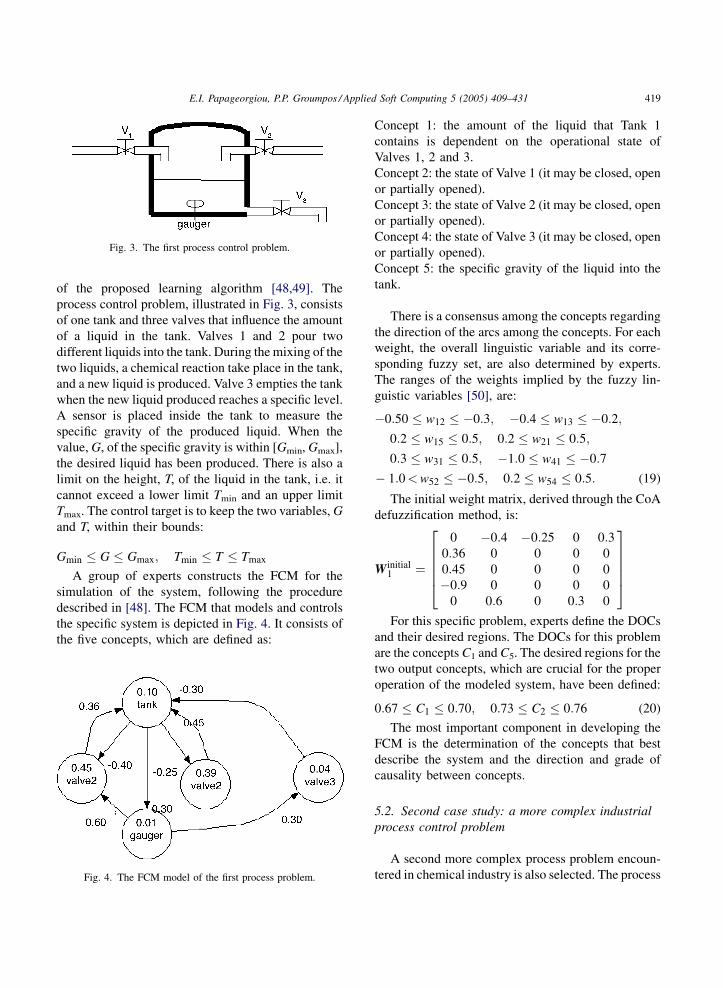
Fig. 3. The first process control problem.
of the proposed learning algorithm [48,49]. The
process control problem, illustrated in Fig. 3, consists
of one tank and three valves that influence the amount
of a liquid in the tank. Valves 1 and 2 pour two
different liquids into the tank. During the mixing of the
two liquids, a chemical reaction take place in the tank,
and a new liquid is produced. Valve 3 empties the tank
when the new liquid produced reaches a specific level.
A sensor is placed inside the tank to measure the
specific gravity of the produced liquid. When the
value, G, of the specific gravity is within [Gmin, Gmax],
the desired liquid has been produced. There is also a
limit on the height, T, of the liquid in the tank, i.e. it
cannot exceed a lower limit Tmin and an upper limit
Tmax. The control target is to keep the two variables, G
and T, within their bounds:
Gmin � G � Gmax; Tmin � T � Tmax
A group of experts constructs the FCM for the
simulation of the system, following the procedure
described in [48]. The FCM that models and controls
the specific system is depicted in Fig. 4. It consists of
the five concepts, which are defined as:
Fig. 4. The FCM model of the first process problem.
Concept 1: the amount of the liquid that Tank 1
contains is dependent on the operational state of
Valves 1, 2 and 3.
Concept 2: the state of Valve 1 (it may be closed, open
or partially opened).
Concept 3: the state of Valve 2 (it may be closed, open
or partially opened).
Concept 4: the state of Valve 3 (it may be closed, open
or partially opened).
Concept 5: the specific gravity of the liquid into the
tank.
There is a consensus among the concepts regarding
the direction of the arcs among the concepts. For each
weight, the overall linguistic variable and its corre-
sponding fuzzy set, are also determined by experts.
The ranges of the weights implied by the fuzzy lin-
guistic variables [50], are:
�0:50 � w12 � �0:3; �0:4 � w13 � �0:2;
0:2 � w15 � 0:5; 0:2 � w21 � 0:5;
0:3 � w31 � 0:5; �1:0 � w41 � �0:7
� 1:0<w52 � �0:5; 0:2 � w54 � 0:5: (19)
The initial weight matrix, derived through the CoA
defuzzification method, is:
Winitial1 ¼
0 �0:4 �0:25 0 0:30:36 0 0 0 0
0:45 0 0 0 0
�0:9 0 0 0 0
0 0:6 0 0:3 0
266664
377775
For this specific problem, experts define the DOCs
and their desired regions. The DOCs for this problem
are the concepts C1 and C5. The desired regions for the
two output concepts, which are crucial for the proper
operation of the modeled system, have been defined:
0:67 � C1 � 0:70; 0:73 � C2 � 0:76 (20)
The most important component in developing the
FCM is the determination of the concepts that best
describe the system and the direction and grade of
causality between concepts.
5.2. Second case study: a more complex industrial
process control problem
A second more complex process problem encoun-
tered in chemical industry is also selected. The process
E.I. Papageorgiou, P.P. Groumpos / Applied Soft Computing 5 (2005) 409–431420
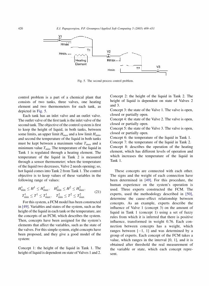
Fig. 5. The second process control problem.
control problem is a part of a chemical plant that
consists of two tanks, three valves, one heating
element and two thermometers for each tank, as
depicted in Fig. 5.
Each tank has an inlet valve and an outlet valve.
The outlet valve of the first tank is the inlet valve of the
second tank. The objective of the control system is first
to keep the height of liquid, in both tanks, between
some limits, an upper limit Hmax and a low limit Hmin,
and second the temperature of the liquid in both tanks
must be kept between a maximum value Tmax and a
minimum value Tmin. The temperature of the liquid in
Tank 1 is regulated through a heating element. The
temperature of the liquid in Tank 2 is measured
through a sensor thermometer; when the temperature
of the liquid two decreases, Valve 2 needs opening; so,
hot liquid comes into Tank 2 from Tank 1. The control
objective is to keep values of these variables in the
following range of values:
H1min � H1 � H1
max; H2min � H2 � H2
max;
T1min � T1 � T1
max; T2min � T2 � T2
max
(21)
For this system, a FCM model has been constructed
in [49]. Variables and states of the system, such as the
height of the liquid in each tank or the temperature, are
the concepts of an FCM, which describes the system.
Then, concepts have been assigned for the system’s
elements that affect the variables, such as the state of
the valves. For this simple system, eight concepts have
been proposed, and they give a good model of the
system:
Concept 1: the height of the liquid in Tank 1. The
height of liquid is dependent on state of Valves 1 and 2.
Concept 2: the height of the liquid in Tank 2. The
height of liquid is dependent on state of Valves 2
and 3.
Concept 3: the state of the Valve 1. The valve is open,
closed or partially open.
Concept 4: the state of the Valve 2. The valve is open,
closed or partially open.
Concept 5: the state of the Valve 3. The valve is open,
closed or partially open.
Concept 6: the temperature of the liquid in Tank 1.
Concept 7: the temperature of the liquid in Tank 2.
Concept 8: describes the operation of the heating
element, which has different levels of operation and
which increases the temperature of the liquid in
Tank 1.
These concepts are connected with each other.
The signs and the weight of each connection have
been determined in [49]. For this procedure, the
human experience on the system’s operation is
used. Three experts constructed the FCM. The
experts, used the methodology described in [50],
determine the cause–effect relationship between
concepts. As an example, experts describe the
influence of Valve 1 (concept 3) on the amount of
liquid in Tank 1 (concept 1) using a set of fuzzy
rules from which it is inferred that there is positive
influence, transformed in weight 0.76. Each con-
nection between concepts has a weight, which
ranges between [�1, 1] and was determined by a
group of experts. Each concept of the FCM takes a
value, which ranges in the interval [0, 1], and it is
obtained after threshold the real measurement of
the variable or state, which each concept repre-
sent.
E.I. Papageorgiou, P.P. Groumpos / Applied Soft Computing 5 (2005) 409–431 421
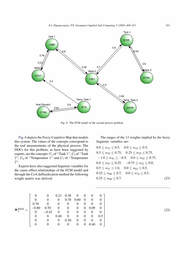
Fig. 6. The FCM model of the second process problem.
Fig. 6 depicts the Fuzzy Cognitive Map that models
this system. The values of the concepts correspond to
the real measurements of the physical process. The
DOCs for this problem, as have been suggested by
experts, are the concepts: C1 of ‘‘Tank 1’’, C2 of ‘‘Tank
2’’, C6 of ‘‘Temperature 1’’ and C7 of ‘‘Temperature
2’’.
Experts have also suggested linguistic variables for
the cause–effect relationships of the FCM model and
through the CoA deffuzification method the following
weight matrix was derived:
W initial2 ¼
0 0 0:21 0:38 0 0 0
0 0 0 0:70 0:60 0 0
0:76 0 0 0 0 0 0
�0:80 0:70 0 0 0 0 0:09
0 �0:42 0 0 0 0 0
0 0 0:40 0 0 0 0
0 0 0 0:30 0 0 0
0 0 0 0 0 0 0:40
266666666664
The ranges of the 13 weights implied by the fuzzy
linguistic variables are:
0:0 � w13 � 0:5; 0:0 � w14 � 0:5;
0:5 � w24 � 0:75; 0:25 � w25 � 0:75;
� 1:0 � w41 � �0:5; 0:0 � w42 � 0:75;
0:0 � w47 � 0:25; �0:75 � w52 � 0:0;
0:5 � w31 � 1:0; 0:0 � w63 � 0:5;
0:25 � w68 � 0:7; 0:0 � w74 � 0:5;
0:25 � w86 � 0:7: (23)
0
0
0
0
0
0:50
0
377777777775
(22)
E.I. Papageorgiou, P.P. Groumpos / Applied Soft Computing 5 (2005) 409–431422
For the FCM model of the process control problem,
all values of concepts are changed synchronously, at
the same iteration step. The desired regions for the
DOCs, which reflect the proper operation of the
modeled system, have been prespecified:
0:5 � C1 � 0:7; 0:75 � C2 � 0:8;
0:65 � C6 � 0:70; 0:65 � C7 � 0:70: (24)
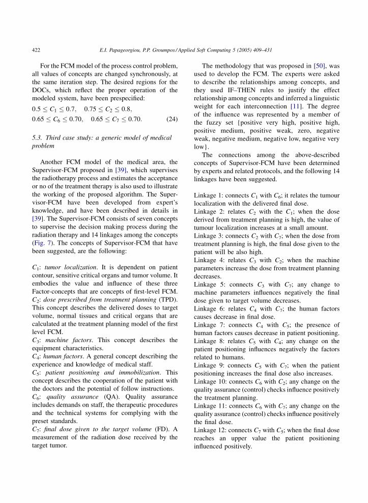
5.3. Third case study: a generic model of medical
problem
Another FCM model of the medical area, the
Supervisor-FCM proposed in [39], which supervises
the radiotherapy process and estimates the acceptance
or no of the treatment therapy is also used to illustrate
the working of the proposed algorithm. The Super-
visor-FCM have been developed from expert’s
knowledge, and have been described in details in
[39]. The Supervisor-FCM consists of seven concepts
to supervise the decision making process during the
radiation therapy and 14 linkages among the concepts
(Fig. 7). The concepts of Supervisor-FCM that have
been suggested, are the following:
C1: tumor localization. It is dependent on patient
contour, sensitive critical organs and tumor volume. It
embodies the value and influence of these three
Factor-concepts that are concepts of first-level FCM.
C2: dose prescribed from treatment planning (TPD).
This concept describes the delivered doses to target
volume, normal tissues and critical organs that are
calculated at the treatment planning model of the first
level FCM.
C3: machine factors. This concept describes the
equipment characteristics.
C4: human factors. A general concept describing the
experience and knowledge of medical staff.
C5: patient positioning and immobilization. This
concept describes the cooperation of the patient with
the doctors and the potential of follow instructions.
C6: quality assurance (QA). Quality assurance
includes demands on staff, the therapeutic procedures
and the technical systems for complying with the
preset standards.
C7: final dose given to the target volume (FD). A
measurement of the radiation dose received by the
target tumor.
The methodology that was proposed in [50], was
used to develop the FCM. The experts were asked
to describe the relationships among concepts, and
they used IF–THEN rules to justify the effect
relationship among concepts and inferred a linguistic
weight for each interconnection [11]. The degree
of the influence was represented by a member of
the fuzzy set {positive very high, positive high,
positive medium, positive weak, zero, negative
weak, negative medium, negative low, negative very
low}.
The connections among the above-described
concepts of Supervisor-FCM have been determined
by experts and related protocols, and the following 14
linkages have been suggested.
Linkage 1: connects C1 with C6; it relates the tumour
localization with the delivered final dose.
Linkage 2: relates C2 with the C1; when the dose
derived from treatment planning is high, the value of
tumour localization increases at a small amount.
Linkage 3: connects C2 with C7; when the dose from
treatment planning is high, the final dose given to the
patient will be also high.
Linkage 4: relates C3 with C2; when the machine
parameters increase the dose from treatment planning
decreases.
Linkage 5: connects C3 with C7; any change to
machine parameters influences negatively the final
dose given to target volume decreases.
Linkage 6: relates C4 with C7; the human factors
causes decrease in final dose.
Linkage 7: connects C4 with C5; the presence of
human factors causes decrease in patient positioning.
Linkage 8: relates C5 with C4; any change on the
patient positioning influences negatively the factors
related to humans.
Linkage 9: connects C5 with C7; when the patient
positioning increases the final dose also increases.
Linkage 10: connects C6 with C2; any change on the
quality assurance (control) checks influence positively
the treatment planning.
Linkage 11: connects C6 with C7; any change on the
quality assurance (control) checks influence positively
the final dose.
Linkage 12: connects C7 with C5; when the final dose
reaches an upper value the patient positioning
influenced positively.

E.I. Papageorgiou, P.P. Groumpos / Applied Soft Computing 5 (2005) 409–431 423
Linkage 13: connects C7 with C1; any change in final
dose causes change in tumour localization.
Linkage 14: connects C7 with C2; when the final dose
increases to an acceptable value, the dose from
treatment planning increases to a desired one.
After the determination of the linkages among c-
oncepts, three radiotherapists-doctors (experts) sug-
gested the fuzzy linguistic variables for the weights of
the linkages, and through the corresponding member-
ship functions [39], the bounds for these weights have
been defined:
0:3 � w17 � 0:5; 0:2 � w21 � 0:4
0:5 � w27 � 0:8; �0:5 � w32 � �0:2;
� 0:5 � w37 � 0; �0:5 � w45 � �0:2;
� 0:6 � w47 � �0:2; �0:6 � w54 � 0:0;
0:4 � w57 � 0:8; 0:5 � w62 � 0:75;
0:5 � w67 � 0:7; 0:0 � w71 � 0:4;
0:5 � w72 � 0:9; 0:5 � w75 � 0:9 (25)
These linguistic variables were defuzzified and
transformed in numerical weights using the construc-
tion methodology of FCMs. Thus, the following
weight matrix for the Supervisor-FCM was produced:
W initial3 ¼
0 0 0 0 0 0 0:50:4 0 0 0 0 0 0:60 �0:3 0 0 0 0 �0:25
0 0 0 0 �0:3 0 �0:30 0 0 �0:4 0 0 0:60 0:55 0 0 0 0 0:5
0:3 0:7 0 0 0:55 0 0
2666666664
3777777775
Also, the desired limits for the parameters TPD and
FD, which represent the Treatment Planning Dose and
the Final Dose, respectively, have been determined by
the three radiotherapists-doctors and the related ICRU
and IAEA protocols [9,19,20], and they are the control
objectives of the Supervisor-FCM. The desired limits
for these parameters are:
0:90 � FD � 0:98; (26)
0:85 � TPD � 0:95; (27)
The Supervisor-FCM evaluates the success or
failure of the treatment by monitoring the values of FD
and TPD concepts. Successful treatment corresponds
to values of the final dose and dose from treatment
planning that lie within the desired bounds. These
values identify the supervisor model [20,34]. The
Supervisor-FCM can be incorporated to an integrated
two-level hierarchical decision making system for the
description and determination of the specific treatment
outcome and for the scheduling of the treatment
process before its treatment execution [20]. Thus,
optimizing the Supervisor-FCM, i.e., detecting the
weights that correspond to the maximum values of the
concepts FD and TPD, within their prespecified
ranges, the result is an enhanced control system which
models the radiotherapy procedure more accurately
and makes decision-making more reliable.
The detection of the optimum FCM’s weights that
correspond to the maximum value of the parameters
FD and TPD, within prescribed ranges, is the
important task. The parameters FD and TPD are
determined as the desired output concepts. For this
purpose, the DE algorithm has been used for the
optimization of the Supervisor-FCM, through the
minimization of an objective function.
The fitness function for this problem, of each
individual weight matrix Wi, can be straightforwardly
defined as:
FðWiÞ ¼ �FDðW iÞ � TPDðWiÞ (28)
where FD(Wi) and TPD(Wi) are the values of the final
dose and the dose prescribed from the treatment
planning, respectively, that correspond to the weight
matrix Wi. The minus signs are used to transform the
maximization problem to its equivalent minimization
problem. Thus, the main optimization problem under
consideration is the minimization of the objective
function F(Wi), such that the constraints of Eqs.
(26) and (27) hold.
The weight matrix W can, in general, be
represented by a vector, which consists of the rows
of W in turn, excluding the elements of the main
diagonal, w11, . . ., wNN, which are by definition equal
to zero:
W¼½w12; . . . ;w1N ;w21; . . . ;w2N ; . . . ;wN1; . . . ;wN;N�1�:
In the Supervisor-FCM, the experts determined 14
linkages and thus, the corresponding minimization
problem is 14-dimensional. The fuzzy linguistic
variables, describing the cause–effect relationships
E.I. Papageorgiou, P.P. Groumpos / Applied Soft Computing 5 (2005) 409–431424
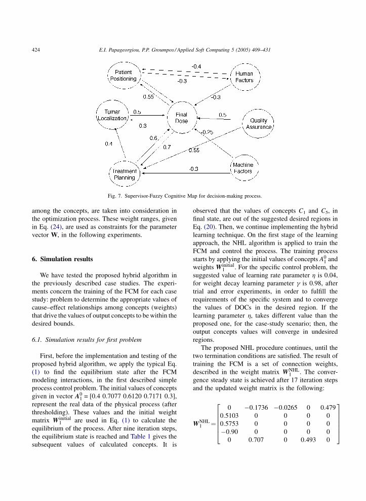
Fig. 7. Supervisor-Fuzzy Cognitive Map for decision-making process.
among the concepts, are taken into consideration in
the optimization process. These weight ranges, given
in Eq. (24), are used as constraints for the parameter
vector W, in the following experiments.
6. Simulation results
We have tested the proposed hybrid algorithm in
the previously described case studies. The experi-
ments concern the training of the FCM for each case
study: problem to determine the appropriate values of
cause–effect relationships among concepts (weights)
that drive the values of output concepts to be within the
desired bounds.
6.1. Simulation results for first problem
First, before the implementation and testing of the
proposed hybrid algorithm, we apply the typical Eq.
(1) to find the equilibrium state after the FCM
modeling interactions, in the first described simple
process control problem. The initial values of concepts
given in vector A01 = [0.4 0.7077 0.6120 0.7171 0.3],
represent the real data of the physical process (after
thresholding). These values and the initial weight
matrix W initial1 are used in Eq. (1) to calculate the
equilibrium of the process. After nine iteration steps,
the equilibrium state is reached and Table 1 gives the
subsequent values of calculated concepts. It is
observed that the values of concepts C1 and C5, in
final state, are out of the suggested desired regions in
Eq. (20). Then, we continue implementing the hybrid
learning technique. On the first stage of the learning
approach, the NHL algorithm is applied to train the
FCM and control the process. The training process
starts by applying the initial values of concepts A01 and
weights Winitial1 . For the specific control problem, the
suggested value of learning rate parameter h is 0.04,
for weight decay learning parameter g is 0.98, after
trial and error experiments, in order to fulfill the
requirements of the specific system and to converge
the values of DOCs in the desired region. If the
learning parameter h, takes different value than the
proposed one, for the case-study scenario; then, the
output concepts values will converge in undesired
regions.
The proposed NHL procedure continues, until the
two termination conditions are satisfied. The result of
training the FCM is a set of connection weights,
described in the weight matrix WNHL1 . The conver-
gence steady state is achieved after 17 iteration steps
and the updated weight matrix is the following:
WNHL1 ¼
0 �0:1736 �0:0265 0 0:479
0:5103 0 0 0 0
0:5753 0 0 0 0
�0:90 0 0 0 0
0 0:707 0 0:493 0
266664
377775
E.I. Papageorgiou, P.P. Groumpos / Applied Soft Computing 5 (2005) 409–431 425
Table 1
The values of concepts at each step of FCM interaction
Steps Tank 1 Valve 1 Valve 2 Valve 3 Cauger
1 0.40 0.7077 0.612 0.717 0.30
2 0.5701 0.6743 0.6253 0.6921 0.6035
3 0.6157 0.6918 0.6184 0.7054 0.6845
4 0.6244 0.7019 0.6141 0.7132 0.7046
5 0.6252 0.7058 0.6125 0.7160 0.7093
6 0.6249 0.7071 0.6121 0.7168 0.7103
7 0.6248 0.7075 0.6120 0.7171 0.7105
8 0.6247 0.7076 0.6120 0.7171 0.7105
9 0.6247 0.7077 0.6120 0.7171 0.7105
which leads the FCM to the following desired state:
C1 ¼ 0:6830; C2 ¼ 0:7632; C3 ¼ 0:6538;
C4 ¼ 0:7534; C5 ¼ 0:7440
Some of the weights have changed significantly their
values from the initial ones in order to succeed the
desired output values of concepts. More specifically, the
weights w31, w52 and w47, have updated their values at a
significant amount to satisfy the constraints for DOCs.
These new values for weights describe new cause–
effect relationships between the concepts of FCM.
Now, the second stage of the Algorithm 1 is implied
and the FCM is retrained by the DE algorithm. The
preliminary solution available by the NHL seeds the
DE and the population is initialised in the neighbour-
hood of the WNHL1 and within the suggested weight
constraints.
Default fixed values of the mutation and crossover
constants (DE parameters) were used; values m = 0.5
and CR = 0.5 have been selected after a trial and error
process. The population size has been always equal to
50. For each algorithm variant, 100 independent
experiments have been performed, to enforce the
reliability of the results, and the algorithm was
allowed to perform 1000 iterations (generations) per
experiment. The best weight matrix detected in these
regions, in terms of its fitness function value F (i.e. the
matrix that corresponds to the smallest fitness function
value) is:
Woptim1 ¼
0 �0:35 �0:20 0 0:40
0:40 0 0 0 0
0:50 0 0 0 0
�0:80 0 0 0 0
0 0:75 0 0:20 0
266664
377775
which leads the FCM to the desired state:
C1 ¼ 0:6723; C2 ¼ 0:7417; C3 ¼ 0:6188;
C4 ¼ 0:6997; C5 ¼ 0:7311
that clearly satisfies the constraints for both C1 and C5,
defined in Eq. (20).
It is clear from the obtained results that there is a
significant divergence for some of the weights from
the initial weight values suggested by the experts.
Only, the weights w21, w31, and w13 keep almost the
same values with the initial ones. Thus the weight
adaptation method adjusts the FCM cause–effect
relationships and controls the values of DOCs to be
within the accepted regions.
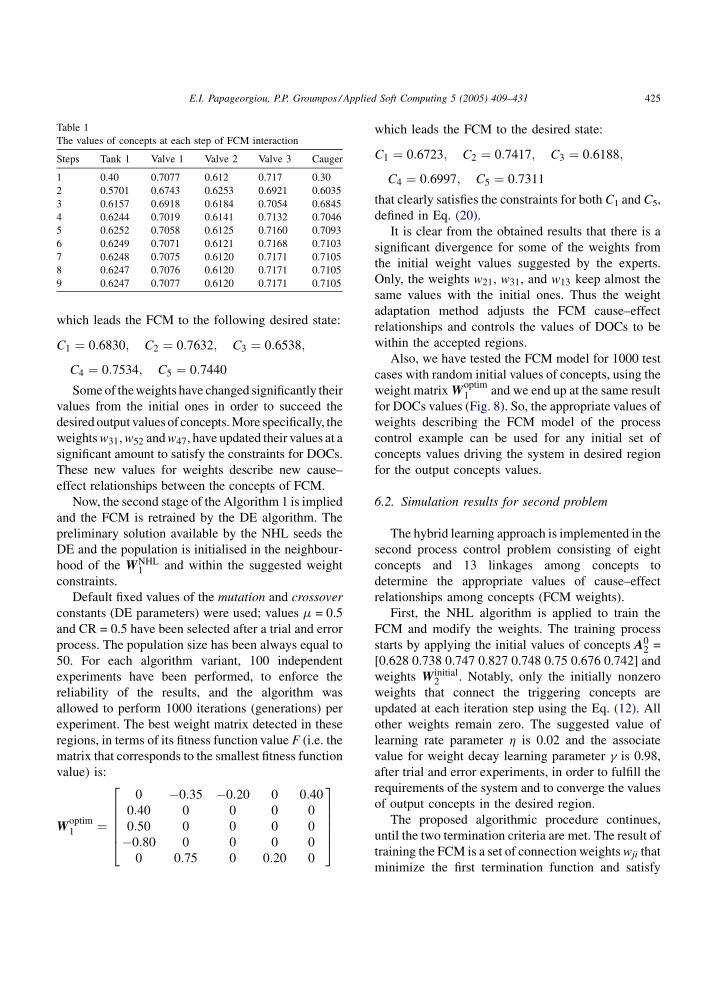
Also, we have tested the FCM model for 1000 test
cases with random initial values of concepts, using the
weight matrix Woptim1 and we end up at the same result
for DOCs values (Fig. 8). So, the appropriate values of
weights describing the FCM model of the process
control example can be used for any initial set of
concepts values driving the system in desired region
for the output concepts values.
6.2. Simulation results for second problem
The hybrid learning approach is implemented in the
second process control problem consisting of eight
concepts and 13 linkages among concepts to
determine the appropriate values of cause–effect
relationships among concepts (FCM weights).
First, the NHL algorithm is applied to train the
FCM and modify the weights. The training process
starts by applying the initial values of concepts A02 =
[0.628 0.738 0.747 0.827 0.748 0.75 0.676 0.742] and
weights Winitial2 . Notably, only the initially nonzero
weights that connect the triggering concepts are
updated at each iteration step using the Eq. (12). All
other weights remain zero. The suggested value of
learning rate parameter h is 0.02 and the associate
value for weight decay learning parameter g is 0.98,
after trial and error experiments, in order to fulfill the
requirements of the system and to converge the values
of output concepts in the desired region.
The proposed algorithmic procedure continues,
until the two termination criteria are met. The result of
training the FCM is a set of connection weights wji that
minimize the first termination function and satisfy
E.I. Papageorgiou, P.P. Groumpos / Applied Soft Computing 5 (2005) 409–431426
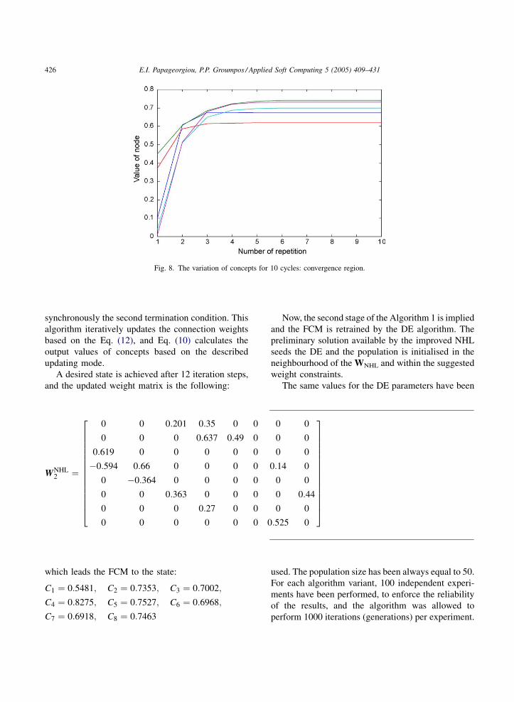
Fig. 8. The variation of concepts for 10 cycles: convergence region.
synchronously the second termination condition. This
algorithm iteratively updates the connection weights
based on the Eq. (12), and Eq. (10) calculates the
output values of concepts based on the described
updating mode.
A desired state is achieved after 12 iteration steps,
and the updated weight matrix is the following:
WNHL2 ¼
0 0 0:201 0:35 0 0 0 0
0 0 0 0:637 0:49 0 0 0
0:619 0 0 0 0 0 0 0
�0:594 0:66 0 0 0 0 0:14 0
0 �0:364 0 0 0 0 0 0
0 0 0:363 0 0 0 0 0:44
0 0 0 0:27 0 0 0 0
0 0 0 0 0 0 0:525 0
266666666666664
377777777777775
which leads the FCM to the state:
C1 ¼ 0:5481; C2 ¼ 0:7353; C3 ¼ 0:7002;
C4 ¼ 0:8275; C5 ¼ 0:7527; C6 ¼ 0:6968;
C7 ¼ 0:6918; C8 ¼ 0:7463
Now, the second stage of the Algorithm 1 is implied
and the FCM is retrained by the DE algorithm. The
preliminary solution available by the improved NHL
seeds the DE and the population is initialised in the
neighbourhood of the WNHL and within the suggested
weight constraints.
The same values for the DE parameters have been
used. The population size has been always equal to 50.
For each algorithm variant, 100 independent experi-
ments have been performed, to enforce the reliability
of the results, and the algorithm was allowed to
perform 1000 iterations (generations) per experiment.
E.I. Papageorgiou, P.P. Groumpos / Applied Soft Computing 5 (2005) 409–431 427
The appropriate weight matrix detected in these
regions, in terms of its fitness value F in Eq. (18)
and accomplishing the initial expert’s suggestions
is:
Wappropriate2 ¼
0 0 0:404 0:554 0 0 0 0
0 0 0 0:636 0:438 0 0 0
0:303 0 0 0 0 0 0 0
�0:554 0:553 0 0 0 0 0:11 0
0 �0:49 0 0 0 0 0 0
0 0 0:375 0 0 0 0 0:38
0 0 0 0:24 0 0 0 0
0 0 0 0 0 0 0:10 0
266666666666664
377777777777775
which leads the FCM to the desired state:
C1 ¼ 0:586; C2 ¼ 0:7026; C3 ¼ 0:7813;
C4 ¼ 0:8565; C5 ¼ 0:7224; C6 ¼ 0:6797;
C7 ¼ 0:6856; C8 ¼ 0:7284
that clearly satisfies the constraints for all four output
concepts, defined in Eq. (24).
It is clear from the obtained results that there are
div-ergences for some of the weights from the initial
weight values suggested by the experts. Only, the
weights w24, w47, and w63 keep near values with the
initial ones.
WNHL3 ¼
0 0 0 0 0 0 0:54
0:465 0 0 0 0 0 0:61
0 �0:100 0 0 0 0 �0:11
0 0 0 0 �0:105 0 �0:078
0 0 0 �0:23 0 0 0:611
0:409 0:681 0 0 0:54 0 0
2666666664
3777777775
(29)
The derived weight matrix Wappropriate2 represents
the appropriate cause–effect relationships among
concepts of the specific FCM model.
6.3. Simulation results for third problem
Before the implementation and testing of the
proposed hybrid algorithm, the initial values of
concepts given in vector A03 = [0.4 0.67 0.3 0.25
0.32 0.4 0.35] and the initial weight matrix Winitial3 are
used in Eq. (1) to calculate the .equilibrium state of the
process.
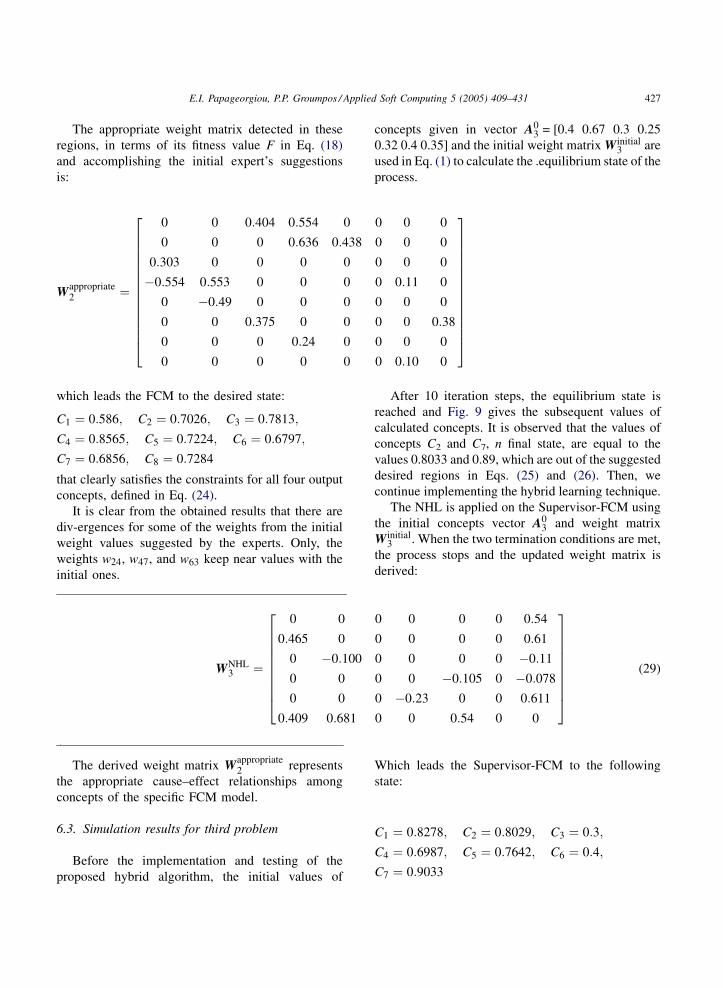
After 10 iteration steps, the equilibrium state is
reached and Fig. 9 gives the subsequent values of
calculated concepts. It is observed that the values of
concepts C2 and C7, n final state, are equal to the
values 0.8033 and 0.89, which are out of the suggested
desired regions in Eqs. (25) and (26). Then, we
continue implementing the hybrid learning technique.
The NHL is applied on the Supervisor-FCM using
the initial concepts vector A03 and weight matrix
Winitial3 . When the two termination conditions are met,
the process stops and the updated weight matrix is
derived:
Which leads the Supervisor-FCM to the following
state:
C1 ¼ 0:8278; C2 ¼ 0:8029; C3 ¼ 0:3;
C4 ¼ 0:6987; C5 ¼ 0:7642; C6 ¼ 0:4;
C7 ¼ 0:9033
E.I. Papageorgiou, P.P. Groumpos / Applied Soft Computing 5 (2005) 409–431428
Fig. 9. Equilibrium state for Supervisor-FCM model.
Then, the process continues implementing the DE
algorithm. The same default fixed values of the
mutation and crossover constants (DE parameters)
with the previous experiments were used. The
population size was the same (50) and 100 independent
experiments have been performed, to enforce the
reliability of the results. Each algorithm was allowed to
perform 1000 iterations (generations) per experiment.
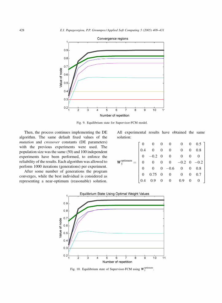
After some number of generations the program
converges, while the best individual is considered as
representing a near-optimum (reasonable) solution.
Fig. 10. Equilibrium state of Supe
All experimental results have obtained the same
solution:
Woptimum3 ¼
0 0 0 0 0 0 0:5
0:4 0 0 0 0 0 0:8
0 �0:2 0 0 0 0 0
0 0 0 0 �0:2 0 �0:2
0 0 0 �0:6 0 0 0:8
0 0:75 0 0 0 0 0:7
0:4 0:9 0 0 0:9 0 0
2666666666664
3777777777775
rvisor-FCM using Woptimum3 .
E.I. Papageorgiou, P.P. Groumpos / Applied Soft Computing 5 (2005) 409–431 429
which leads the FCM to the desired state given in
Fig. 10. We observe that in the equilibrium state the
values of output concepts are C2 = 0.8777 and
C7 = 0.9482.
It is clear that the values of C2 and C7 lie within the
desired regions defined by Eqs. (25) and (26), while the
weights fulfil the ranges posed initially by the group of
experts. This supports the claim that the obtained
solution is the true optimal solution. Some of the
weights have changed significantly their values from
the initial ones in order to succeed the desired output
values of concepts. We remark that there is a very high
positive influence of the concept C7 (final dose) to the
concept C2 (dose prescribed from the treatment
planning) as well as to the concept C5 (patient
positioning). This means that if we succeed to deliver
the maximum dose to the target volume; then, the initial
calculated dose from treatment planning is the desired
and the same happens with the patient positioning. It
must be mentioned that the estimated weights take their
optimum values at the edges of the suggested bounds.
The optimal values of FD and TPD are acceptable
according to the ICRU and IAEA protocols [19,20].
Thus, radiotherapists can follow the suggested
values and the treatment will be executed with
successful results. The proposed approach is efficient
and very useful for the FCM-controlled clinical
radiotherapy process. The recalculation of all weights
that participate in the simulation process constitutes the
most important drawback of the simple FCM model as
initially determined by experts-doctors. Its importance
to the radiotherapists is underlined by the fact that they
will be able to introduce clinical cases based on a range
of accepted values for the output concepts of the model.
The limitations of our work are the following.
� E
xperts should know the proper operation of thesystem or the desired behavior of problem in order
to provide certain regions for the values of output
concepts.
� N
o new interconnections are derived using theproposed learning technique and there is not any
influence on the architecture of the FCM model.
Future experiments and trials can overcome these
limitations. For the specific problems, the experts had
known the proper operations for the problem and the
derived weight matrices are the optimum ones.
7. Conclusions
A new hybrid method to train Fuzzy Cognitive
Maps, based on a two stage learning approach, first
stage the nonlinear Hebbian learning algorithm and
second stage the differential evolution algorithm, has
been developed, tested and applied in three problems
with different complexity levels.
Three real-life problems with increasing complex-
ity levels have been used for the illustration of the
proposed learning algorithm. The results appear to be
very promising, verifying the effectiveness of the
learning procedure. The physical meaning of the
obtained results is retained. Using the proposed
learning procedure, the deficiencies of FCMs, such
as the potential convergence to undesired states for the
output concepts values overcome. Also, the FCM
might change its fuzzy causal web as causal patterns
change and as experts update their causal knowledge.
In this work, it is also investigated how well novel
and easy to understand evolutionary algorithms,
referred to as differential evolution (DE) algorithms,
and claimed to be very efficient when they are applied
to solve optimization problems. The results show that
the DE algorithms are very robust, effective and highly
efficient in solving the studied class of process control
problems. Thus they are able of mitigating the
drawback of long computation times commonly
associated with evolutionary algorithms.
Simulation results suggest that the new method
exhibits fast and stable learning, good generalization,
and therefore, a great possibility of good performance.
The proposed algorithm is able to train Fuzzy
Cognitive Maps fast and efficiently, determining the
appropriate weight matrix that leads the values of
output concepts within desired convergence regions.
Future work is directed towards more investigation
on evolutionary computation techniques and the
development of new learning techniques for adapting
FCM causal links.
References
[1] J. Aguilar, Adaptive random fuzzy cognitive maps, in: F.J.
Garijio, J.C. Riquelme, M. Toro (Eds.), IBERAMIA 2002,
Lecture Notes in Artificial Intelligence, 2527, Springer-Ver-
lag, Berlin, Heidelberg, 2002, pp. 402–410.

E.I. Papageorgiou, P.P. Groumpos / Applied Soft Computing 5 (2005) 409–431430
[2] P. Angeline, Tracking extrema in dynamic environments, sixth
Annual Conference on Evolutionary Programming VI,
Springer, 1997, pp. 335–345.
[3] R. Axelrod, Structure of Decision, The Cognitive Maps of
Political Elites, Princeton University Press, Princeton, New
Jersey, 1976, p. 404.
[4] T. Back, H.P. Schwefel, An overview of evolutionary algorithms
for parameter optimization, Evol. Comput. 1 (1993) 1–23.
[5] T. Back, Evolutionary Algorithms in Theory and Practice,
Oxford University Press, New York, 1996.
[6] T. Back, D. Fogel, Z. Michalewicz, Handbook of Evolutionary
Computation, IOP Publishing and Oxford University Press,
New York, 1997.
[7] P. Bartlett, T. Downs, Training a Neural Network Using a
Genetic Algorithm, Tech. Report, Department of Electrical
Engineering, University of Queensland, 1990;
H.G. Beyer, H.P. Schwefel, Evolution strategies: a compre-
hensive introduction, Nat. Comput. 1 (1) (2002) 3–52.
[8] N.L. Biggs, E.K. Llooyd, R.J. Wilson, Graph Theory 1736–
1936, Clarendon Press, Oxford, 1976.
[9] A. Brahme, Optimization of radiation therapy, Int. J. Radiat.
Oncol. Biol. Phys. 28 (1994) 785–787.
[10] J.P. Craiger, D.F. Goodman, R.J. Weiss, A.B. Butler, Modelling
organizational behaviour with Fuzzy Cognitive Maps, Int. J.
Comput. Intell. Org. 1 (1996) 120–123.
[11] N. Dodd, Optimization of network structure using genetic
techniques, in: Proceedings of the 1990 International Joint
Conference on Neural Networks, 1990.
[12] D. Fogel, Evolutionary Computation: Towards a new Philo-
sophy of Machine Learning, IEEE Press, Piscataway, MJ,
1996.
[13] F. Harary, R.J. Norman, D. Cartwright, Structural Models: An
Introduction to the Theory of Directed Graphs, John Wiley &
Sons, New York, 1965, p. 201.
[14] M. Hassoun, Fundamentals of Artificial Neural Networks,
MIT Press, Bradford Book, Massachusetts, 1995.
[15] S. Haykin, Neural Networks: A Comprehensive Foundation,
second ed. Macmillan, 1994.
[16] D.O. Hebb, The Organization of Behaviour: A Neuropsycho-
logical Theory, John Wiley, New York, 1949.
[17] J. Heistermann, Learning in neural nets by genetic algorithms,
in: R. Eckemiller, G. Hartmann, G. Hauske (Eds.), Parallel
Processing in Neural Systems and Computers, Elsevier, 1990,
pp. 165–168.
[18] R. Horst, H. Tuy, Global Optimization: Deterministic
Approaches, Springer, New York, 1996.
[19] ICRU Report 50, Prescribing, recording and reporting photon
beam therapy, International Commission on Radiation Units
and Measurements, Washington, 1993.
[20] IAEA, Radiation dose in radiotherapy from prescription to
delivery, IAEA-TECDOC-734, 1994.
[21] J.S.R. Jang, C.T. Sun, E. Mizutani, Neuro-Fuzzy and Soft
Computing, N.J. Prentice-Hall, Upper Saddle River, 1997.
[22] S. Khan, A. Chong, T.A. Gedeon, Methodology for developing
adaptive fuzzy cognitive maps for decision support, in: Pro-
ceedings of the Third Australia–Japan Evolutionary Systems,
Canberra, 23–25 November, 1999, pp. 93–100.
[23] B. Kosko, Fuzzy Cognitive Maps, Int. J. Man-Mach. Stud. 24
(1986) 65–75.
[24] B. Kosko, Neural Networks and Fuzzy Systems, Prentice-Hall,
New Jersey, 1992.
[25] M. Li, H.-Y. Tam, Hybrid evolutionary search method based on
clusters, IEEE Trans. On Pattern Analysis and Machine Intel-
ligence 23 (8) (2001) 786–799.
[26] C.T. Lin, C.S.G. Lee, Neural Fuzzy Systems: A Neuro-Fuzzy
Synergism to Intelligent Systems, N.J. Prentice Hall, Upper
Saddle River, 1996.
[27] Z.Q. Liu, R. Satur, Contextual fuzzy cognitive map for deci-
sion support in geographic information systems, IEEE Trans.
Fuzzy Syst. 5 (1999) 495–507.
[28] I.L. Lopez Cruz, L.G. Van Willigenburg, G. Van Straten,
Efficient differential evolution algorithms for multimodal
optimal control problems, Appl. Soft Comput. 3 (2003) 97–
122.
[29] G.D. Magoulas, V.P. Plagiannakos, M.N. Vrahatis, Neural
network-based colonoscopic diagnosis using on-line learning
and differential evolution, Appl. Soft Comput. 4 (4) (2004)
357–367.
[30] Y. Miao, Z.Q. Liu, On causal inference in fuzzy cognitive
maps, IEEE Trans. Fuzzy Syst. 8 (2000) 107–119.
[31] E. Oja, Neural networks, principal components and subspaces,
Int. J. Neural Syst. 1 (1989) 61–68.
[32] E. Oja, H. Ogawa, J. Wangviwattana, Learning in nonlinear
constrained Hebbian networks, in: T. Kohonen, et al. (Eds.),
Artificial Neural Networks, Amsterdam, North-Holland, 1991,
pp. 385–390.
[33] E.I. Papageorgiou, C.D. Stylios, P.P. Groumpos, Activation
Hebbian learning rule for fuzzy cognitive Maps, in: Proceed-
ings of the Fifteenth IFAC World Congress of International
Federation of Automatic Control, Barcelona, Spain, July 21–
26, 2002, CD-ROM.
[34] E. Papageorgiou, C. Stylios, P. Groumpos, An integrated two-
level hierarchical decision making system based on Fuzzy
Cognitive Maps (FCMs), IEEE Trans. Biomed. Eng. 50 (12)
(2003) 1326–1339.
[35] E.I. Papageorgiou, C.D. Stylios, P. Spyridonos, G. Nikiforidis,
P.P. Groumpos, Urinary bladder tumour grading using non-
linear Hebbian learning for Fuzzy Cognitive Maps, in: Procee-
ings of the IEE International Conference on Systems
Engineering (ICSE 2003), 2, 2003, 542–547.
[36] E.I. Papageorgiou, C.D. Stylios, P.P. Groumpos, Fuzzy cog-
nitive map learning based on nonlinear Hebbian rule, in: T.D.
Gedeon, L.C.C. Fung (Eds.), AI 2003, Lecture Notes in
Artificial Intelligence 2903, Springer-Verlag, Berlin Heidel-
berg, 2003, pp. 254–266.
[37] E.I. Papageorgiou, C.D. Stylios, P.P. Groumpos, Active Heb-
bian learning algorithm to train fuzzy cognitive maps, Int. J.
Approx. Reason. 37 (3) (2004) 219–247.
[38] E.I. Papageorgiou, K.E. Parsopoulos, P.P. Groumpos, M.N.
Vrahatis, Fuzzy cognitive maps learning through swarm intel-
ligence, in: International Conference on Artificial Intelligence
and Soft Computing, Zakopane, Poland, 7–11 June, Lecture
Notes in Artificial Intelligence 3070, Springer Verlag, Berlin
Heidelberg, 2004, pp. 344–349.
E.I. Papageorgiou, P.P. Groumpos / Applied Soft Computing 5 (2005) 409–431 431
[39] E.I. Papageorgiou, P.P. Groumpos, Optimization of fuzzy
cognitive map model in clinical radiotherapy through differ-
ential evolution algorithm, Biomed. Soft Comput. Hum. Sci. 9
(2) (2004).
[40] C.E. Pelaez, B.J. Bowles, Using fuzzy cognitive maps as a
system model for failure modes and effects analysis, Inf. Sci.
88 (1996) 177–199.
[41] K.V. Price, An introduction to differential evolution, in: D.
Corne, M. Dorigo, F. Glover (Eds.), New Ideas in Optimiza-
tion, McGraw-Hill, New York, 1999.
[42] J.C.F. Pujol, R. Poli, Evolving the topology and the weights of
neural networks using a dual representation, Appl. Intell. 8
(1998) 73–84.
[43] H.P. Schwefel, Numerical Optimization of Computer models,
Wiley, Chichester, 1981.
[44] H.P. Schwefel, Evolution and Optimum Seeking, Wiley, New
York, 1995.
[45] R. Storn, On the Usage of Differential Evolution for Function
Optimization, NAFIPS, Berkely, 1996, pp. 519–523.
[46] R. Storn, K. Price, Minimizing the real functions of the
ICEC’96 contest by differential evolution, in: Proceedings
of the IEEE Conference on Evolutionary Computation,
Nagoya, 1996, pp. 842–844.
[47] R. Storn, K. Price, Differential evolution: a simple and efficient
heuristic for global optimization over continuous spaces, J.
Global Optimization 11 (1997) 341–359.
[48] C.D. Stylios, P.P. Groumpos, V.C. Georgopoulos, An fuzzy
cognitive maps approach approach to process control systems,
J. Adv. Comput. Intell. 3 (5) (1999) 409–417.
[49] C.D. Stylios, P.P. Groumpos, Fuzzy cognitive maps in model-
ling supervisory control systems, J. Intell. Fuzzy Syst. 8 (2000)
83–98.
[50] C.D. Stylios, P.P. Groumpos, Modelling Fuzzy Cognitive
Maps, IEEE Trans. Syst. Man Cybern. Part A 34 (1) (2004)
155–162.
[51] A. Tiwari, R. Roy, G. Jared, O. Munaux, Evolutionary-based
techniques for real-life optimization: development and testing,
Appl. Soft Comput. 1 (4) (2002) 301–329.
[52] G. Weiss, Towards the synthesis of neural and evolutionary
learning, in: O. Omidvar (Ed.), Progress in Neural Networks,
5, Ablex Pub, 1993 Chapter 5.
[53] G. Weiss, Neural networks and evolutionary computation, part
I: hybrid approaches in artificial intelligence, in: Proceedings
of ICEC, 1993.
[54] G. Weiss, Neural networks and evolutionary computation, part
II: hybrid approaches in neurosciences, in: Proceedings of the
IEEE World Congress on Computational Intelligence, 1993.
[55] W.R. Zhang, S.S. Chen, W. Wang, R.S. King, A cognitive map
based approach to the coordination of distributed cooperative
agents, IEEE Trans. Syst. Man Cybern. 22 (1) (1992) 103–114.
[56] J. Zurada, Introduction to Artificial Neural Systems, West
Publishing Company, 1992.