Train-Induced Ground Vibration and Its Prediction
183
TRITA-JOB PHD 1005 ISSN 1650-9501 Train-Induced Ground Vibration and Its Prediction Mehdi Bahrekazemi Division of Soil and Rock Mechanics Dept. of Civil and Architectural Engineering Royal Institute of Technology Stockholm 2004
-
Upload
khangminh22 -
Category
Documents
-
view
1 -
download
0
Transcript of Train-Induced Ground Vibration and Its Prediction

TRITA-JOB PHD 1005 ISSN 1650-9501
Train-Induced Ground Vibration and Its Prediction
Mehdi Bahrekazemi
Division of Soil and Rock Mechanics Dept. of Civil and Architectural Engineering
Royal Institute of Technology Stockholm 2004


Errata
Train-Induced Ground Vibration and Its Prediction
Mehdi Bahrekazemi
Page Line Printed Correct 2 16 f.t. model to model too 2 17 f.t. form sites from sites 14 last tow events two events 14 4 f.b. criterion criteria 15 Fig. 2-9,
cap. criterion criteria
15 Fig. 2-9, cap.
(1997).quality (1997)
15 Fig. 2-10, cap.
Figure 2-9.quality Figure 2-9
16 15 f.b. Fel! Hittar inte referenskälla Equation 2-3 17 19 f.b. methods used that methods that 18 17 f.b. (With & Bahrekazemi, 2003) (With et al., 2004) 20 19 f.t. Some times sometimes 21 6 f.t. three dimensional three-dimensional 22 last 2-9 2-9 to Table 2-11 23 3 f.b. for four 24 Fig. 2-13 RMS partivle velocity RMS particle velocity 27 2 f.b. type train type of train 28 6 f.t. levels running levels for trains running 49 3 f.b. about above 53 6 f.t. 70 kPa 30 kPa 54 19 f.t. place at placed at 57 14 f.b. 15 kPa in the top layer and
increases to about 45 kPa 20 kPa in the top layer and increases to about 22 kPa
61 7 f.b. bellow below 67 1 f.t. chapter 0 chapter 3 68 5 f.t. 1.2 and 2.4 1.2 % and 2.4 % 69 9 f.b. For this purpose For the purpose of this 70 1 f.t. HISTOEIES HISTORIES 70 2 f.t. running running r.m.s. 71 7 f.t. same as same, as 73 7 f.t. a criteria a criterion 74 9 f.b. Figure 4-15 in Figure 4-15 86 7 f.b. speed as shown speed. As shown 87 1 f.t. mediumhas medium has 90 1 f.b. strait straight 96 Figure 4-
45 [(mm/s)(kN] [(mm/s)/kN]
97 5 f.b. on the natural frequencies of the building in different directions
on the modal shapes in different directions at the natural frequencies of the building
99 2 f.t. chapter 0 chapter 3 99 9 f.t. verifyd verified 99 14 f.b. chapter 1 chapter 4 105 11 f.t. chapter 0 chapter 3 105 8 f.b. chapter 0 chapter 3 106 Table 5-
1 b [(mm/s)/(km/h)] b [mm/s]
108 Figure 5-13
Particle vlocity in the track the track
Particle velocity in the track
118 6 f.t. F and out F and output 120 Eq. 6-1 ))(,(Η+)(= τθτθ equ ))G(q, y(t) )(,(Η+)(= teqtu ))G(q, y(t) θθ 121 6 f.t. & 9
f.t. error criterion error
121 Eq. 6-9 )|()(),( θθε tytyt −= )|(ˆ)(),( θθε tytyt −= 124 1 f.t. & 3
f.t. near field near-field
126 Eq. 6-12 ( )∑ −⋅⋅= iiiio tvDRtv τψζ ),()( 0 ( )∑ −⋅⋅= iiiio tvRRtv τψζ ),()( 0
126 5 f.b. ),( 0 ii DRψ ),( 0 ii RRψ 131 9 f.t. superposed superimposed 144 Figure 6-
31, cap. bellow below
153 18 f.b. The most important effect the The most important effect of the155 12 f.b. to does to those 155 10 f.b. near-filed near-field 159 13 f.b. &
17 f.b. Iournal Journal
160 5 f.b. Bodare, A. (2003) Mätningar Bodare, A. (2004) Mätningar everywhere one second rms / one-second
rms / one-second-r.m.s one-second-r.m.s.
Add to the references
Lai, C. G., Callerio, A., Faccioli, E., Martino, A. (2000) Mathematical modeling of railway-induced ground vibrations, proceedings of the international workshop Wave 2000, Bochum, Germany, 13-15 December 2000, pp. 99-110.

To my family


Mehdi Bahrekazemi
v
FOREWORD This thesis is based on the first phase of a project named ENVIB, the Environmental Effects of Train-Induced Ground Vibrations. The project that is financed by Swedish Railway Administration (Banverket) consists of two phases, each one two years and will continue until December 2005. The first phase of the project has been carried out from December 2001 to December 2003 at the division of Soil and Rock Mechanics, department of Civil and Architectural Engineering, Royal Institute of Technology in Stockholm, Sweden. The objective of this phase is to develop a semi-empirical model for prediction of ground-borne vibration due to train traffic. This work has become possible thanks to the help and support the author has been receiving. Gratitude is extended to Swedish Railway Administration (Banverket), for financing the ENVIB project and to the Division of Soil and Rock Mechanics at KTH for providing a professional and friendly work environment. The author would also like to thank Norwegian Geotechnical Institute, NGI for their valued cooperation in providing parts of the measurement data. Thanks are also forwarded to all colleagues at the Soil and Rock Mechanics Div. especially to senior lecturer Anders Bodare for his appreciated management of the project and helpful advices during this time, and Professor Håkan Stille for his valuable support and advices throughout these years. The author would also like to express his sincere appreciation for the help and support he has received from Mr. Alexander Smekal (Banverket) and the ENVIB project’s reference group members, Dr. Christian Madshus (NGI), Dr. Lars Olsson (VBB & GEOSTATISTIK), and Mr. Eric Berggren (Banverket). Dr. Bo Andréasson from WSP Sverige AB, Göteborg is also thanked for his help and valuable advices. Dr. Kent Lindgren from the MWL at KTH is thanked for his help in performing the measurements, as well as Dr. Robert Hildebrand, Elis Svensson, Per Delin, Thomas Engberg and Therese Bergh Hansson for their help during some of these measurements. Thanks are also forwarded to the Seismological Dept. of University of Uppsala for letting us borrow the seismometers used for the measurements presented in this thesis. Special thanks are forwarded to the Elleman Family from Partille for their hospitality and cooperation during the measurements at the Partille test site. Professor Friedrich Quiel from the Div. of Environment and Natural Resources at KTH is thanked for his advices and help on the GIS system, and Docent Mikael

Train-Induced Ground Vibration and Its Prediction
vi
Johansson from the Institution of Signals, Sensors & Systems at KTH for his appreciated consultation during preparation of the part on system identification. At the end the reader should notice that the section of “Glossary of Symbols” have been excluded from this thesis as the symbols are locally explained for each equation presented throughout the thesis. Stockholm, January 2004 Mehdi Bahrekazemi

Mehdi Bahrekazemi
vii
SUMMARY Besides high maintenance costs due to excessive vibration in the track, ground-borne vibration due to train traffic may cause annoyance to people who live nearby the track or interfere with the operation of sensitive equipment inside the buildings. Consequently despite the fact that ground-borne vibration from train traffic usually do not cause damage to the buildings, the economical and environmental aspects of the issue justify careful assessment of the problem prior to constructing new railway tracks or upgrading the existing ones for heavier and faster traffic. It is in this context that a model for prediction of train-induced ground-borne vibration can be useful. This thesis is based on the first two years of a four-year project named ENVIB. The objective of the project which is financed by the Swedish Railway Administration, (Banverket) is to study the ground-borne vibration induced in the environment by train traffic. The purpose of the project is to expand the existing experiences in making predictions about ground-borne vibration. Based on the present situation of ground-borne vibration due to traffic of passenger and freight trains on existing railways, it shall be possible to predict the future conditions of ground-borne vibration in case of an increase in speed and axle load of the trains. Any model for prediction of ground-borne vibration due to train traffic must include at least three main components. These three main components, which themselves may include many different parts are the source, propagation path, and the receiver. Depending on how detailed these three components are defined, and how accurate the predictions made by the model are, they can be classified into three different classes. The first class (class I) includes scoping models that should be used at the earliest phase of the project to primarily identify those parts along the track that may have excessive ground-borne vibration. The second class (class II) includes those models that are more accurate than class I and are suitable for the purpose of quantifying the severity of the problem more precisely. Finally, those models that have the best accuracy and can be used to support the design and specification of the track and possible mitigation measures are classified as class III. This thesis presents a series of measurements which are performed or their results have been used in the framework of the ENVIB project. Some general conclusions from the measurements have been discussed and a class I semi-empirical model based on the measurement data has been presented. The model can be integrated into a GIS system in order to study large areas and thereby choose the best possible position of a new railway. The model can even be used in
Train-Induced Ground Vibration and Its Prediction
viii
order to make it possible for trains with different axle loads (for example freight trains with different axle loads) to have the highest possible speed on the existing railway tracks through densely populated areas without causing excessive ground-borne vibration. This model has been presented in form of an equation and a table containing the needed parameters to be used for different types of trains on different soil conditions. Furthermore a class II semi-empirical model is suggested which can be used in order to study the problem in a more accurate way at those locations that have been identified by the first model. This model is based on a library of sub-models that can be put together to make a specially made confectionary model suitable for each site and case. There are only a few objects available in the model’s different libraries for the time being, but as more measurement data from new sites become available, more objects can be added to the model. Both models have been verified using data that have not been used for development of them. The verification shows that there is good agreement between the prediction and the measurement for both the class I and class II models.

Mehdi Bahrekazemi
ix
SAMMANFATTNING Förutom ökade kostnader för underhåll av en bana kan markvibrationer orsakade av tågtrafik uppfattas som störande av människor som bor i närheten av spåret, eller störa driften av vibrationskänsliga instrument i intilliggande byggnader. Som en konsekvens av detta och trots att tåginducerade markvibrationer normalt inte orsakar allvarliga skador på byggnader, borde denna frågeställning undersökas från ekonomiska men framförallt miljömässiga synpunkter innan några nya banor byggs eller de befintliga banorna uppgraderas för tyngre och fortare trafik. Det är i detta sammanhang en modell som kan ge prognoser om vibrationsförhållandena på grund av tågtrafik kan användas. Denna avhandling baseras på de två första åren av ett fyrårigt projekt kallad ENVIB. Projektet Finansieras av Banverket och har som mål att undersöka miljöpåverkan av tåginducerade markvibrationer. Syftet med projektet är att utvidga de erfarenheter som idag finns för att prognostisera skakningar av marken eller en byggnads grund. Prognosen skall kunna användas för ordinarie person och godstrafik idag till de förhållanden som kommer att råda vid en ev. uppgradering av befintliga banor för höjda tåghastigheter och axellaster. Det ingår dessutom att beskriva olika typer av åtgärder som kan vidtas om skakningarna bedöms som oacceptabla. Varje modell som ska användas för prognostisering av tåginducerade markvibrationer måste på något sätt ta hänsyn till tre olika länkar. De tre länkarna som själva kan bestå av flera delar är källan, mottagaren, och vägen mellan källan och mottagaren. Beroende på hur komplicerade och detaljerade länkarna har beskrivits inom modellen och hur noggrant prognosen kan bli, delas modellerna in i tre olika klasser. Den första klassen (klass I) innehåller de modeller som ger en översikt över problemet och kan användas i den allra tidigaste fasen av projektet för att få en översikt över de delar av banan som kan ha problem med för höga markvibrationer. Den andra klassen (klass II) omfattar de modeller som är noggrannare än den första och kan kvantifiera graden av problemet med bättre noggrannhet. Till sist, klassas de modeller som har den absolut bästa noggrannheten och kan ge underlag för dimensionering av banan och ev. vibrationsminskande åtgärder till klass III. Denna avhandling presenterar en rad mätningar som har gjorts och/eller vars resultat har använts inom ramen av projektet ENVIB. En del allmänna slutsatser från mätningarna har diskuterats och en semiempirisk modell av klass I baserat på mätdata har presenterats. Modellen kan användas tillsammans med ett GIS system

Train-Induced Ground Vibration and Its Prediction
x
för att undersöka stora områden och där bestämma den bästa möjliga positionen för en ny bana. Modellen kan även användas för att göra det möjligt för tåg med olika axellaster (t ex godståg med olika axellaster) at köra med högsta möjliga hastighet på de befintliga banorna genom tätbefolkade områden utan att orsaka för höga markvibrationer. Denna modell presenteras i form av en ekvation och en tabell som innehåller de parametrar som används i samband med användning av ekvationen för olika typer av tåg och markförhållanden. Ytterligare ges ett förslag på en modell av klass II som kan användas för att studera problemet på ett noggrannare sätt i de områden som har identifierats av den första modellen. Denna modell baseras på ett bibliotek av submodeller som kan sättas ihop av användaren för att skräddarsy en modell anpassad till varje område och fall. För närvarande finns det bara ett fåtal objekt i biblioteket men i takt med att mer mätdata från flera områden blir tillgängliga, kan flera objekt läggas till biblioteket. Båda modellerna har verifierats med data som inte har använts tidigare för framtagningen av dem. Verifieringarna visar god överensstämmelse mellan prognos och mätdata både för modell klass I och klass II.

Mehdi Bahrekazemi
xi
TABLE OF CONTENTS
FOREWORD............................................................................................. V
SUMMARY ............................................................................................. VII
SAMMANFATTNING............................................................................... IX
TABLE OF CONTENTS .......................................................................... XI
1 INTRODUCTION ................................................................................1
1.1 Background.......................................................................................................................1
1.2 Objectives..........................................................................................................................2
1.3 Structure of the thesis ......................................................................................................2
2 STATE OF THE ART..........................................................................5
2.1 ground-borne vibration due to train traffic ...................................................................5 2.1.1 Vibration source ............................................................................................................5 2.1.2 Propagation path ............................................................................................................9 2.1.3 Receiver.......................................................................................................................11
2.2 Effects of Vibration ........................................................................................................11 2.2.1 Human response ..........................................................................................................11 2.2.2 Vibration effects on sensitive equipment.....................................................................14 2.2.3 Vibration impacts on buildings....................................................................................16
2.3 Mitigation Methods ........................................................................................................17 2.3.1 Mitigation methods in the source ................................................................................17 2.3.2 Mitigation methods in the path ....................................................................................18 2.3.3 Mitigation methods in the building..............................................................................18
2.4 Prediction Models...........................................................................................................19 2.4.1 How should the model look like? ................................................................................20
2.4.1.1 Different classes of models ................................................................................20 2.4.1.2 General structure of a model ..............................................................................21
2.4.2 Models suggested by DOT-T-95-16 and DOT-293630-1............................................21 2.4.3 Norwegian model ........................................................................................................28 2.4.4 Other models ...............................................................................................................30
Train-Induced Ground Vibration and Its Prediction
xii
2.5 Discussion and conclusions............................................................................................ 33
3 MEASUREMENTS ...........................................................................35
3.1 Data acquisition and processing.................................................................................... 35 3.1.1 Measurement equipment used for KTH measurements............................................... 37
3.2 Measurements Performed by KTH .............................................................................. 42 3.2.1 Ledsgård ...................................................................................................................... 42
3.2.1.1 Geotechnical condition of the site...................................................................... 43 3.2.1.2 Measurements .................................................................................................... 44
3.2.2 Säbylund...................................................................................................................... 49 3.2.2.1 Geotechnical condition of the site...................................................................... 49 3.2.2.2 Measurements .................................................................................................... 51
3.2.3 Partille, Kåhög............................................................................................................. 52 3.2.3.1 Geotechnical condition of the site...................................................................... 53 3.2.3.2 Measurements .................................................................................................... 54
3.2.4 Partille, Eckensvägen .................................................................................................. 57 3.2.4.1 Geotechnical condition of the site...................................................................... 57 3.2.4.2 Measurements .................................................................................................... 58
3.3 Measurements Performed by Others............................................................................ 61 3.3.1 Ledsgård ...................................................................................................................... 61 3.3.2 Finland, Koria.............................................................................................................. 61
3.3.2.1 Geotechnical condition of the site...................................................................... 62 3.3.2.2 Measurements .................................................................................................... 63
4 ANALYSIS OF MEASUREMENT DATA..........................................67
4.1 Determining speed of trains........................................................................................... 67
4.2 Wheel force ..................................................................................................................... 69
4.3 normalized one-second-r.m.s. of time histoeies............................................................ 70
4.4 Different directional components of vibration............................................................. 72
4.5 Different sensors used for vibration measurement ..................................................... 73
4.6 Location of the sensor .................................................................................................... 78 4.6.1 Comparing vibration in the ballast with sleeper .......................................................... 78 4.6.2 Vibration at similar locations along the track.............................................................. 81 4.6.3 Attenuation of vibration with distance from track centerline ...................................... 83
4.7 Effect of wheel/train load on ground-borne vibration ................................................ 88
4.8 Effect of train speed on ground-borne vibration......................................................... 89
4.9 Effect of train type on ground-borne vibration ........................................................... 91
4.10 Effect of train length on ground-borne vibration........................................................ 91
4.11 Effect of geotechnical conditions on ground-borne vibration .................................... 91
4.12 Vibration in buildings .................................................................................................... 97
4.13 Effect of some countermeasures.................................................................................... 97
Mehdi Bahrekazemi
xiii
4.14 Summary of conclusions from the measurements .......................................................97
5 ENVIB SEMI-EMPIRICAL MODEL, CLASS I ..................................99
5.1 The structure of the model and its parameters............................................................99
5.2 Verification of the model .............................................................................................107
5.3 Integrating the model with a GIS system ...................................................................111 5.3.1 Definition of GIS.......................................................................................................111 5.3.2 GIS Software .............................................................................................................112 5.3.3 ENVIB’s GIS system.................................................................................................113 5.3.4 An example of using the model within the GIS system.............................................115
5.4 Discussion and conclusions ..........................................................................................115
6 ENVIB SEMI-EMPIRICAL MODEL, CLASS II ...............................117
6.1 Subsystems ....................................................................................................................117 6.1.1 Sub-model I, track .....................................................................................................120
6.1.1.1 Modeling subsystem I ......................................................................................120 6.1.1.2 Some examples ................................................................................................121
6.1.2 Sub-model II, near field.............................................................................................124 6.1.3 Sub-model III, path....................................................................................................125
6.1.3.1 Point sources ....................................................................................................128 6.1.3.2 Gamma distribution of the path length.............................................................130 6.1.3.3 Geometrical and material damping ..................................................................131 6.1.3.4 Some examples of suitable damping parameters..............................................134
6.1.4 Sub-model IV, building .............................................................................................141 6.1.4.1 Transfer function of a building at Partille ........................................................142
6.2 Verification of the Model .............................................................................................146
6.3 Discussion......................................................................................................................151
7 DISCUSSION AND CONCLUSIONS .............................................153
7.1 General conclusions......................................................................................................153
7.2 Suggestion for future work..........................................................................................155
REFERENCES ......................................................................................157
APPENDICES........................................................................................161
APPENDIX A, “USER MANUAL” of the ENVIB CLASS II MOdel, ENVIB01.................161
APPENDIX B, Typical Response curves of the sensors ..........................................................165
APPENDIX C, SOME DEFINITIONS.....................................................................................167

Mehdi Bahrekazemi
1
1 INTRODUCTION
1.1 BACKGROUND Although ground–borne vibration from train traffic is very unlikely to cause damage to the buildings and structures, the economical and environmental aspects of the issue deserve careful consideration. Besides high maintenance cost due to excessive vibration in the railway structure, ground-borne vibration may cause annoyance to the people living near the railway or interfere with the operation of sensitive equipment. Therefore preparing an environmental impact assessment prior to building new railway lines through densely populated areas or upgrading the existing ones to be trafficked by heavier or faster trains is becoming more common nowadays. A ground vibration prediction model is a tool that can properly be used in different phases of railway design process and preparing such environmental impact assessment. Using the model one can study the problem and propose mitigation methods if necessary during each phase. As the numerical models are very time consuming regarding the capacity and speed of the available computers and even computers that will come in the next 10 years, there is a need to develop simple empirical or analytical models for studying the effect of train traffic on ground-borne vibration in the vicinity of the railway. On the other hand analytical models are mostly suitable for very simple cases where both the geometry and geotechnical conditions of the problem are not too complicated. Therefore empirical or semi-empirical models are usually used in order to predict ground-borne vibration due to train traffic especially in the preliminary phase of the projects when high accuracy in the prediction is not needed. The prediction models can be classified in three classes as suggested by ISO/CD 14837-1 (2001) depending on the accuracy of the prediction made by them. The first class is the scoping model that should be used at the earliest stage of the development of a project. The purpose of this kind of models is to identify problem with ground-borne vibration and the areas with the most severe problem. This type of models is helpful especially when deciding on the location of new tracks. The model is usually very simple and quick to use and requires very few input parameters that are available in the first stage of development process of project. These parameters are for example type of the railway system and the

Train-Induced Ground Vibration and Its Prediction
2
trains that are going to run on the track, typical geotechnical conditions of the ground and the sensitivity of the nearby buildings to ground-borne vibration. The preliminary design models used in the early phase of railway design are the next class of models. These models are suitable for quantifying the severity of the problem with ground-borne vibration and identifying its location along the railway more accurately than the scoping models. Finally the third class of models used for prediction of ground-borne vibrations is the detailed design models that are used as part of the design process after the location of the track has been decided on. This type of models can be used to quantify the problem or the result of the mitigation work for a specific section along the track.
1.2 OBJECTIVES The main objective of the work upon which this thesis is based is developing an empirical model based on measurement data from train-induced ground vibration. The form of the model and its parameters will be chosen so that the most important aspects of the issue are considered without making the model to complicated or impractical. As the available measurement data are form sites with very soft to soft clay, the model will be most appropriate to be used for similar conditions. Nevertheless this will not be a serious disadvantage for the model as the problem of excessive ground-borne vibration due to train traffic is normally encountered at sites with such geotechnical conditions. Considering the wide range of opportunities offered by geographical information systems, GIS it has been decided to make the model capable of being integrated into such systems. This way the calculations will be performed within the GIS system and the result will be presented on the geographical map of the area as contour lines. In order to avoid very long running times that makes the GIS system impractical, a class I model will be used for this purpose. On the other hand a class II model may be used to study in more details those locations along the railway that have been identified by the GIS system as places with risk for excessive ground-borne vibration. A class II model will also be suggested in this thesis.
1.3 STRUCTURE OF THE THESIS
This thesis comprises of 7 main chapters that are as following. The first chapter that includes even this section is an introduction trying to give the reader some background on the subject of train-induced ground vibration, states the objectives of this thesis, and reviews its structure. The second chapter covers a brief review of the state of the art with the purpose of presenting a summary of the current knowledge about the subject of this thesis. The third chapter presents the measurements whose data have been used for this work, including both those performed by the author and those which have been carried out by some other parties but made available to the author. The fourth chapter presents some analysis done on the measurement data as well as general conclusions drawn from
Mehdi Bahrekazemi
3
them. The fifth chapter is about the first semi-empirical model presented in this thesis as well as a GIS system suggested to be integrated with the model. Chapter six suggests another semi-empirical model which is based on a sub-model philosophy. The model is suggested to be divided into several sub-models presented in the form of several libraries of sub-models so that the user can make his / her own model by putting together the appropriate sub-models from their library. Although a section presenting the conclusions from each chapter is provided at the end of each chapter, chapter 7 is devoted to the discussion and conclusions about the whole thesis. A list of the references used throughout the thesis is presented after chapter 7 followed by appendices that cover the material that seems necessary for the thesis to be complete but did not have a place in the main text.


Mehdi Bahrekazemi
5
2 STATE OF THE ART In this chapter a brief review of the state of the art on the subject of ground-borne vibration due to train traffic and its prediction is presented. The generation of the vibration at the “source”, its “propagation” through the “medium” and reception by the “receiver” is discussed. Furthermore vibration effects on humans, sensitive equipment and buildings are reviewed, and some methods usually used for vibration mitigation are introduced. Finally some of the models used currently to make predictions on train-induced ground vibration are briefly reviewed.
2.1 GROUND-BORNE VIBRATION DUE TO TRAIN TRAFFIC In general it can be said that the problem of excessive ground-borne vibration due to train traffic has three links, i.e. the source, the path and the receiver as schematically shown in Figure 2-1. Understanding how each of these three links influence the vibration situation is crucial in prediction and mitigation of the problem. In the rest of this section each of these three links are discussed briefly while the interested reader is referred to a literature survey by Bahrekazemi and Hildebrand (2000), for further study.
2.1.1 Vibration source Generally it is believed that the vibration is generated due to interaction of the moving train with the track which lies on the underlying soil. The main parts of the train from the point of view of vibration generation are schematically shown in Figure 2-2. The car body is connected to the bogie via the secondary
Figure 2-1. The three links of the ground-borne vibration problem.

Train-Induced Ground Vibration and Its Prediction
6
suspension which usually in case of modern passenger trains consists of an air bag. The weight of the car body is then transferred to the wheels via a bogie frame that is connected to the wheels by the primary suspension system. The wheels in turn transfer the load to the rails as shown by Figure 2-3. The vertical forces Vr and Vl comprise of six different parts or contributions as given by Equation 2-1 (Andersson et al. 2002). These different parts are given in table
jdbdhdsk FVFVFVFVFVFVFV +++++= 0 Equation 2-1
Table 2-1. Different parts of the vertical force applied on the rails from wheels. The forces are normalized with respect to the static wheel force. The number in the size column shows the normalized contribution of each force to the total vertical force.
Contribution to the total force Designation size Static wheel force FV0 100% Quasi-static contribution in curves FVk 0-40% Dynamic contribution due to rail roughness FVds 0-300%Dynamic contribution due to wheel flat FVdh 0-300%Contribution due to braking FVdb 0-20% Contribution due to asymmetries FVj 0-10%
Car body
Primarysuspension
SecondarysuspensionWheel
Bogie frame Figure 2-2. Main parts of a train bogie.
FVlFVr
FHl FHr
FVl
FHl FHr
FVr Figure 2-3. Vertical and horizontal contact force between wheel and rail, (Andersson et al., 2002).

Mehdi Bahrekazemi
7
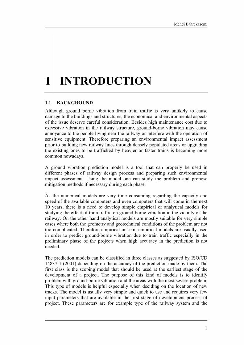
Figure 2-4 shows different parts of the track in a schematic way. As seen in the figure the railway track consists of the rails, rail pads and rail fasteners, sleepers, ballast, and sub-ballast. Depending on the type of the traffic, different parts of the track may have different specifications. In Sweden, depending on the track class and design specifications of the railway, track specifications are given according to Table 2-2. The fastener shown in detail A of the Figure 2-4 is of type Pandrol (P, according to Table 2-2) with 10 mm rubber as the rail pad. This type of fastener is the standard type used for all new railways with concrete sleepers in many countries in Europe.
Sub ballast
BallastSleeper
Rail
Railway track
CL
Underlying soil orembankment
A
Sleeper
RailRail clips
Rail pad
(Andersson et al. 2002)Detail A Figure 2-4. Schematic picture of railway track and description of its different parts.
Table 2-2. Specifications of different parts of the track depending on track class, and type of traffic according to BVF 524.1 (Andersson et al. 2002).
Sleeper Design parameters Track class Rails Fasteners
Material Distance [cm]
Ballast Stax [ton]
Sth [km/h]
Stvm [ton/m]
I UIC60 P Btg 60-65 M
25 22.5 20 18
50 120 160
>160
12.0 8.1 8.1 8.1
II BV50 B,H,I,P Btg, Bok 50-65 M
25 22.5 20 18
50 100 160
>160
12.0 8.1 8.1 8.1
III BV50 F,L Bok, Furu 65 M 22.5
20 90
130 8.1 8.1
IV SJ43 U Furu 65-75 G,M 22.5 20
70 90
8.1 8.1
P, B, L, H, I, P, F, U= type of the rail fastener according to Figure 2-5. Btg = Concrete, M = Makadam; G = Gravel Stax = Maximum load, Sth = Maximum speed Stvm = Maximum load per meter Notice that the rails are welded in case of class I and class II tracks.
Train-Induced Ground Vibration and Its Prediction
8
R F H
K I P
Figure 2-5. Different types of rail fasteners (Andersson et al., 2002).
According to a review of state of the art by Nelson and Saurenman (1983), ground-borne vibration caused by train traffic is influenced by factors as wheel and rail roughness, discrete track supports, dynamic characteristics of the rolling stock, rail support stiffness, railway structure design, soil characteristics, and building structure design. Dawn and Stanworth (1979), discuss the generation, propagation and reception of vibrations due to train traffic. With respect to generation of the vibrations they recognize both quasi-static and dynamic vibrations, and according to them the vibration energy is not shared equally among the modes and most of the energy is carried by Rayleigh waves at significant distances from the train. It is mentioned that if the train were to travel faster than the propagation velocity of the ground vibration, the shock wave which is formed in the ground would seriously affect the nearby buildings. Experimental results are presented which show a peak at the sleeper passing frequency in a nearby building. It is suggested by them that the excitation of ground vibration, especially at low frequencies, depend on the total vehicle mass, not just the unsprung mass of the wheelset. This is evidenced by a large measured difference between loaded and unloaded trains; the difference in train weights is approximately 12 dB, and the measured vibration difference is approximately the same. Experimental results also show a peak which is explained to be a corrugation-generated tone, with a wavelength of 1.78 m on the rail. Krylov (1995), Madshus et al. (1996), Bodare (1999), Jones et al. (2000), and Degrande and Lombart (2000) are among other authors who have recognized the speed of the train as an important factor that influences the amount of energy transmitted from the track to the surrounding. On the other hand according to Dawn (1983), the ground vibrations from heavy freight trains on good quality welded tracks have only weak dependence on train speed above 30km/h. Hannelius (1974), indicates in a report that the significant frequency range for ground vibration is in the range of 0-10 Hz for cohesive soils, and higher frequencies for soils of friction material. He further notices that vibration in the ground increases with decreasing mass of the bank-fill material, and increasing depth to the bedrock.

Mehdi Bahrekazemi
9
Different source mechanisms may be recognized for vibrations generated at different frequencies. Fujikake (1986), studies the generation of vibrations due to impact during the passage of the wheel over rail joints, and propagation of the resulting vibrations into the ground. According to him peaks in the ground vibration spectra occur at the axle-passing frequency and its overtones. Jones (1994), lists the source mechanisms of vibration from train passages as roughness generated vibration in the track, parametric excitation at the sleeper passing frequency, and quasi-static vibration due to the moving load. Krylov and Ferguson (1994), using a Green’s function formalism, discuss the theory of generation of low-frequency ground vibrations due to quasi-static pressure from the wheels. Considering the soil as elastic foundation, and using the Euler-Bernoulli formula for an elastic beam on an elastic foundation, the generation of vibrations due to passage of the deflection curve from each sleeper and the vibration induced by each sleeper in the ground has been formulated. Expressing that the major part of the energy is carried by Rayleigh waves, only these waves have been considered in determining the spectral density of the vertical vibrations. It has been concluded that vibration spectra strongly depend on the axle load. Remington (1987), presents a model of rail vibration due to roughness on the rails and wheels.
2.1.2 Propagation path After being generated in the track, the vibration propagates to the surrounding through the media. Hannelius (1978), suggests that Rayleigh waves dominate at a distance from the track; while body waves are significant within the first 20 m, approximately. Based on a literature survey, Nelson and Saurenman (1983), present Equation 2-2 for propagation attenuation of waves in linear elastic half space, where n is given by Table 2-3 and, some examples of α are given by Table 2-4. The Rayleigh wave is considered important, especially at greater distances from the track, since the body waves decay more rapidly by geometric spreading than the Rayleigh wave
( )0
00
rrn
errvv −−
−
⋅
⋅= α
Equation 2-2
where, =0v Particle velocity at the source =0r The distance from the source to the reference point on the ground =r The distance from the source to the receiver =n The power of geometric attenuation =α The factor for material damping
Table 2-3. Power of geometric attenuation
Wave Type Point source Line sourceShear waves 1 0.5 Compression waves 1 0.5 Rayleigh waves 0.5 0 Love waves 0.5 0
Train-Induced Ground Vibration and Its Prediction
10
Table 2-4. The factor for material damping, α
Soil Type Soil Attenuation, α [m-1]
Water-saturated clay 0.04 - 0.12 Loess and loessial soil 0.10 Sand and silt 0.04
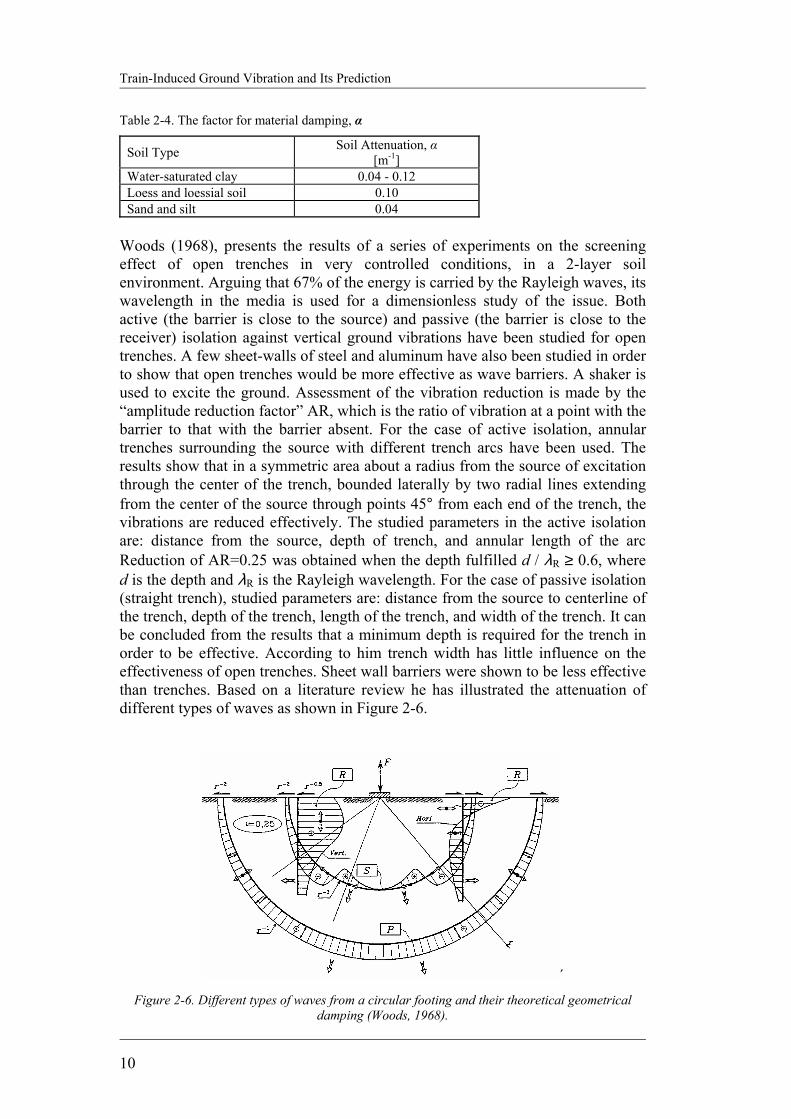
Woods (1968), presents the results of a series of experiments on the screening effect of open trenches in very controlled conditions, in a 2-layer soil environment. Arguing that 67% of the energy is carried by the Rayleigh waves, its wavelength in the media is used for a dimensionless study of the issue. Both active (the barrier is close to the source) and passive (the barrier is close to the receiver) isolation against vertical ground vibrations have been studied for open trenches. A few sheet-walls of steel and aluminum have also been studied in order to show that open trenches would be more effective as wave barriers. A shaker is used to excite the ground. Assessment of the vibration reduction is made by the “amplitude reduction factor” AR, which is the ratio of vibration at a point with the barrier to that with the barrier absent. For the case of active isolation, annular trenches surrounding the source with different trench arcs have been used. The results show that in a symmetric area about a radius from the source of excitation through the center of the trench, bounded laterally by two radial lines extending from the center of the source through points 45° from each end of the trench, the vibrations are reduced effectively. The studied parameters in the active isolation are: distance from the source, depth of trench, and annular length of the arc Reduction of AR=0.25 was obtained when the depth fulfilled d / λR ≥ 0.6, where d is the depth and λR is the Rayleigh wavelength. For the case of passive isolation (straight trench), studied parameters are: distance from the source to centerline of the trench, depth of the trench, length of the trench, and width of the trench. It can be concluded from the results that a minimum depth is required for the trench in order to be effective. According to him trench width has little influence on the effectiveness of open trenches. Sheet wall barriers were shown to be less effective than trenches. Based on a literature review he has illustrated the attenuation of different types of waves as shown in Figure 2-6.
´ Figure 2-6. Different types of waves from a circular footing and their theoretical geometrical
damping (Woods, 1968).
Mehdi Bahrekazemi
11
2.1.3 Receiver After being generated in the track, and propagating through the media, the vibrations are received by the foundations of nearby buildings. From the foundations the vibrations then propagate to the other parts of the buildings. Nelson (1987), has discussed building response to vibration considering the effect of foundation type on transmission of vibrations from the ground to the building and vibration propagation within the building. It has been stated that in multi-story buildings, a common value for the (high-frequency) attenuation of vibration from floor-to-floor is approximately 3 dB. According to Hannelius (1974) resonance of the whole building usually occur below 10 Hz, while resonances of walls and ceilings occur in the 10-60 Hz range. Jones (1994), summarizes the response of the building to the vibrations as typically having resonances of the whole building on the foundation at about 4 Hz, floors at about 20-30 Hz, and walls and windows above 40 Hz. Jonsson (2000), have presented experimental and theoretical investigation carried out to characterize and explain low-frequency ground and structural vibrations related to railway traffic. It has been concluded from a case study that only the low-frequency content of the vibrations is effectively transmitted into the building foundation. According to the author the building has been subjected to loading by a wave field slightly inclined to the railway normal.
2.2 EFFECTS OF VIBRATION After being received by the building foundations, the vibrations are then propagated through other parts of the building. What effects the vibration may have on the occupants inside the building, how the equipment sensitive to vibration will be affected, and finally if there is any risk of damage to the building are the main three questions that arise with this respect. In this section an answer is given to these three questions based on a review of the literature.
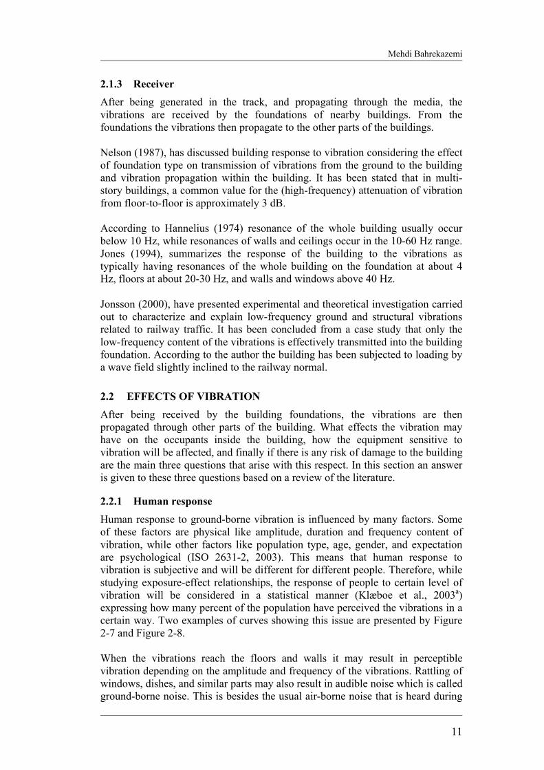
2.2.1 Human response Human response to ground-borne vibration is influenced by many factors. Some of these factors are physical like amplitude, duration and frequency content of vibration, while other factors like population type, age, gender, and expectation are psychological (ISO 2631-2, 2003). This means that human response to vibration is subjective and will be different for different people. Therefore, while studying exposure-effect relationships, the response of people to certain level of vibration will be considered in a statistical manner (Klæboe et al., 2003a) expressing how many percent of the population have perceived the vibrations in a certain way. Two examples of curves showing this issue are presented by Figure 2-7 and Figure 2-8. When the vibrations reach the floors and walls it may result in perceptible vibration depending on the amplitude and frequency of the vibrations. Rattling of windows, dishes, and similar parts may also result in audible noise which is called ground-borne noise. This is besides the usual air-borne noise that is heard during
Train-Induced Ground Vibration and Its Prediction
12
the passage of the train. In fact there is indication of interaction between exposure to noise and vibration from traffic (Klæboe et al., 2003b). People may be more annoyed if they are exposed to both noise and vibration compared to when only vibration is felt.
Figure 2-7. Human response to residential building vibration with 4 to 15 rapid transit trains per
hour (DOT-293630-1).
Per
cent
age
of p
eopl
e
Figure 2-8. The percentage of persons with various degrees of annoyance due to vibrations in dwellings, plotted against calculated statistical maximum values for weighted velocity, vw,95 in
mm/s (NSF, 1999).

Mehdi Bahrekazemi
13
On the issue of appropriate quantity to be used in evaluating human response to ground-borne vibration ISO 2631-1 (1997) suggests the r.m.s. method unless substantial peaks are present in the vibration. For vibrations with such high peaks where the crest factor1 is greater than 9, additional and/or alternative methods are presented. One of these alternative measures suggested by ISO 2631-1 (1997) is the running r.m.s. value2. According to the U.S. Department of Transportation, (1998) the perception threshold of humans for particle velocity is about 0.04 mm/s (65 dB with reference 1e-6 inch/sec). Despite very low perception limit, most people will be annoyed by the ground-borne vibrations only if it has much higher levels as shown by Figure 2-7. The ground-borne noise on the other hand may still be annoying even if the vibration levels are below perception limits. The ground-borne vibration impact criteria for ordinary buildings and special buildings according to US-DOT-293630-1 (1998), has been given in Table 2-5 and Table 2-6 respectively. Table 2-5. Ground-borne vibration (r.m.s. particle velocity) impact criteria according to the U.S. Department of Transportation, DOT-293630-1, (1998).
Ground-borne vibration Impact levels (dB, ref. 1-6
in./sec)
Ground-borne vibration Impact
levels (mm/s) Land Use Category
Frequent eventsa
Infrequent eventsb
Frequent events
Infrequent events
Category 1: building where vibration would interfere with interior operations.
65 65c 0.05 0.05
Category 2: Residence and buildings where people normally sleep.
72 80 0.10 0.25
Category 3: Institutional land uses with primarily daytime use. 75 83 0.14 0.36
Notes: a) Frequent events is defined as more than 70 vibration events per day. b) Infrequent events is defined as fewer than 70 vibration events per day. c) This criterion limit is based on levels that are acceptable for most moderately
sensitive equipment such as optical microscopes. Vibration-sensitive manufacturing or research will require detailed evaluation to define the acceptable vibration levels. Ensuring lowere vibration levels in a building often requires special design of the HVAC systems and stiffened floors.
1 Crest factor of vibration is defined as the ratio of peak value to r.m.s. value (ISO 2041, 1990). 2 For definition see Appendix C, some definitions.

Train-Induced Ground Vibration and Its Prediction
14
The Swedish Railway Administration (Banverket) and the Swedish Environmental Protection Agency (Naturvårdsverket) together have suggested the criterion for Environmental impact of ground-borne vibrations from railway traffic as presented in Table 2-7 (BVPO 724.001, 1997). The values given by this table correspond to the lower limit for moderate disturbance given by SS 460 4861 (1992).
Table 2-7. Ground-borne vibration criterion for environmental impact according to guidelines prepared by Banverket and Naturvårdsverket in Sweden.
Particle Velocity Particle Acceleration Vibration level r.m.s. (1-80 Hz)
0.4 mm/s 14 mm/s2
2.2.2 Vibration effects on sensitive equipment
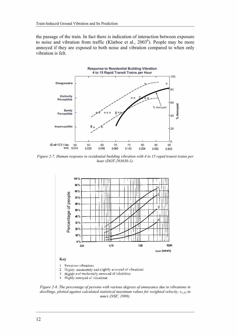
Traffic induced ground vibration may interfere with the performance of sensitive equipment like electron microscopes inside buildings. Therefore it is sometimes necessary to mitigate the vibrations if the railway track passes close to the building. The kind of the suitable countermeasure must be decided on depending on the specific conditions of the track and the building. ISO 10811-1 (2000) and ISO 10811-2 (2000) cover the issues of measurement, evaluation, and classification of vibration and shock in buildings with sensitive equipment. Usually the manufacturer’s guidelines provide the necessary information about the maximum level of vibration for sensitive equipment. In the absence of more reliable information, Figure 2-9 may provide general guidelines about vibration criterion for sensitive equipment. The five different equipment classes as shown by the curves in the figure are explained in Figure 2-10. The criteria for maximum allowed vibration levels for sensitive equipment are based
Table 2-6. Ground-borne vibration (r.m.s. particle velocity) criteria for special buildings according to the U.S. Department of Transportation, (DOT-293630-1, 1998). 1e-6 in./secis used as reference.
Ground-borne vibration Impact levels (dB, ref. 1-
6 in./sec)
Ground-borne vibration Impact levels (mm/s) Type of Building or
Room Frequent eventsa
Infrequent eventsb
Frequent eventsa
Infrequent eventsb
Concert Halls TV Studios Recording Studios Auditoriums Theaters
65 65 65 72 72
65 65 65 80 80
0.05 0.05 0.05 0.10 0.10
0.05 0.05 0.05 0.25 0.25
Notes: a) Frequent events is defined as more than 70 vibration events per day. b) Infrequent events is defined as fewer than 70 vibration events per day.
Mehdi Bahrekazemi
15
on single events. This is due to the fact that it is very unlikely that tow events even if they occur at the same time are exactly cohesive and in phase with each other to be additive.
Figure 2-9. Generic vibration criterion curves, from Amick, (1997). quality
Figure 2-10. Application of criterion curves shown in Figure 2-9. quality

Train-Induced Ground Vibration and Its Prediction
16
2.2.3 Vibration impacts on buildings A review of the reports on vibration related damages to buildings (Nelson & Saurenman, 1983) has shown that there is only 5 % probability that buildings would receive structural damages3 due to particle velocities less than 50 mm/s and no case had been reported of structural damage to buildings for particle velocities less than 25 mm/s. According to the review there is no risk of architectural damage to normal buildings due to vibration less than 15 mm/s. ISO 4866 (1990) gives guidelines for measurement of vibrations and their effects on buildings. According to this standard the duration of the dynamic exciting force is an important parameter as well as frequency and range of vibration intensity. Building related factors to be considered are type and condition of buildings, natural frequencies and damping, building base dimensions, and the soil at the site. The Norwegian standard NS 8141 (NSF, 2001), and the Swedish standard SS 460 48 66 (SEK, 1991) give similar guidelines for allowable peak value of vibration for different kind of buildings, on different soils. While the Swedish standard only deals with explosion induced vibration, the Norwegian Standard is valid even for traffic-induced ground-borne vibration. According to the Norwegian standard the allowable peak value of vibration in order to avoid damage to the buildings is given by Equation 2-3.
kdbg FFFFvv ⋅⋅⋅= .0 Equation 2-3 where, v0 is the uncorrected particle velocity (peak value) which is 20 mm/s. Fg is a factor that accounts for the soil conditions at the building site. Fb is a factor for the type of the building, its material and foundation type. Fd is a factor that considers the distance between the building and the source. Fk is a factor for the type of the source which is equal to 1.0 for traffic. Using Equation 2-3 the minimum peak value of particle velocity induced by traffic (due to construction activities) that may result in architectural damage to an ordinary residential building on very soft clay (the worst case) located 15 m from the source can be calculated to be about 4 mm/s. If a historical building is considered at the same distance, this limit would be about 2 mm/s. These limits are for the worst cases when buildings with very unfavorable type of construction and foundation are built on very soft clay. For comparison the allowable peak particle velocity at 15 m distance from the traffic source in case of a building which is built of reinforced concrete on piles in very soft clay is about 10 mm/s. Experience shows that very seldom ground vibration measured at 15 m from the track centerline would exceed 4 mm/s or even 2 mm/s. In fact it is very unlikely that ground-borne vibration caused by train traffic may result in structural damage of buildings, although in most severe cases it may result in minor cosmetic damage if the buildings are too close to the track. Usually the threshold amplitude for ground-borne vibration that may cause cosmetic damage to buildings is at 3 Structural damage in this report is defined as glass breakage and serious plaster cracking, possibly accompanied by falling plaster.
Mehdi Bahrekazemi
17
least three times higher than the vibration amplitude caused by train traffic at about 15 m from the track centerline (DOT-T-95-16, 1995). Therefore in the rest of this thesis the issue of ground-borne vibration in the building is only studied from the point of view of annoyance to the residents. Consequently the vibration is expressed in r.m.s. unless otherwise stated despite the fact that the cosmetic damage to the building is more correlated with the peak amplitude of vibration. It is worth to mention here that some buildings that are more sensitive to environmental vibrations like theaters, TV studios, concert halls, and laboratories with sensitive equipment should be studied separately and thoroughly whenever a new railway line goes in the vicinity of them.
2.3 MITIGATION METHODS
In order to reduce train induced ground-borne vibration at a distance from the track, several issues such as generation of the vibration at the source, its propagation through the media, and interaction with the structure at the receiver should be considered. In other words the available mitigation methods against excessive ground-borne vibration can be divided into three general groups. The first group includes those that result in less vibration being generated in the source. The second group of countermeasures focuses on the propagation of the vibration from the source to the receiver, and finally the third group of countermeasures includes those methods that reduce the effect of the vibration at the receiver. The best method or methods can therefore be adopted considering technical as well as economical aspects of the problem.
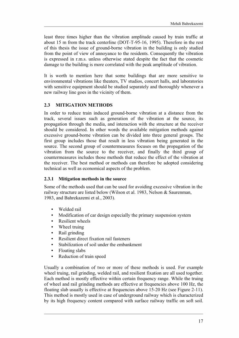
2.3.1 Mitigation methods in the source Some of the methods used that can be used for avoiding excessive vibration in the railway structure are listed below (Wilson et al. 1983, Nelson & Saurenman, 1983, and Bahrekazemi et al., 2003).
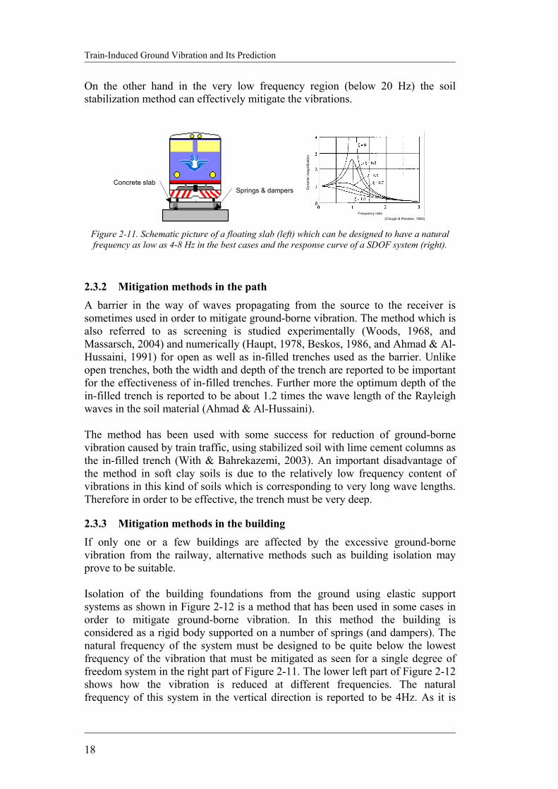
• Welded rail • Modification of car design especially the primary suspension system • Resilient wheels • Wheel truing • Rail grinding • Resilient direct fixation rail fasteners • Stabilization of soil under the embankment • Floating slabs • Reduction of train speed
Usually a combination of two or more of these methods is used. For example wheel truing, rail grinding, welded rail, and resilient fixation are all used together. Each method is mostly effective within certain frequency range. While the truing of wheel and rail grinding methods are effective at frequencies above 100 Hz, the floating slab usually is effective at frequencies above 15-20 Hz (see Figure 2-11). This method is mostly used in case of underground railway which is characterized by its high frequency content compared with surface railway traffic on soft soil.
Train-Induced Ground Vibration and Its Prediction
18
On the other hand in the very low frequency region (below 20 Hz) the soil stabilization method can effectively mitigate the vibrations.
Springs & dampersConcrete slab
Frequency ratio
Dynamic
mag
nific
atio
n
(Clough & Penzien, 1993) Figure 2-11. Schematic picture of a floating slab (left) which can be designed to have a natural frequency as low as 4-8 Hz in the best cases and the response curve of a SDOF system (right).
2.3.2 Mitigation methods in the path
A barrier in the way of waves propagating from the source to the receiver is sometimes used in order to mitigate ground-borne vibration. The method which is also referred to as screening is studied experimentally (Woods, 1968, and Massarsch, 2004) and numerically (Haupt, 1978, Beskos, 1986, and Ahmad & Al-Hussaini, 1991) for open as well as in-filled trenches used as the barrier. Unlike open trenches, both the width and depth of the trench are reported to be important for the effectiveness of in-filled trenches. Further more the optimum depth of the in-filled trench is reported to be about 1.2 times the wave length of the Rayleigh waves in the soil material (Ahmad & Al-Hussaini). The method has been used with some success for reduction of ground-borne vibration caused by train traffic, using stabilized soil with lime cement columns as the in-filled trench (With & Bahrekazemi, 2003). An important disadvantage of the method in soft clay soils is due to the relatively low frequency content of vibrations in this kind of soils which is corresponding to very long wave lengths. Therefore in order to be effective, the trench must be very deep.
2.3.3 Mitigation methods in the building If only one or a few buildings are affected by the excessive ground-borne vibration from the railway, alternative methods such as building isolation may prove to be suitable. Isolation of the building foundations from the ground using elastic support systems as shown in Figure 2-12 is a method that has been used in some cases in order to mitigate ground-borne vibration. In this method the building is considered as a rigid body supported on a number of springs (and dampers). The natural frequency of the system must be designed to be quite below the lowest frequency of the vibration that must be mitigated as seen for a single degree of freedom system in the right part of Figure 2-11. The lower left part of Figure 2-12 shows how the vibration is reduced at different frequencies. The natural frequency of this system in the vertical direction is reported to be 4Hz. As it is

Mehdi Bahrekazemi
19
seen from the frequency spectra provided by the manufacturer the vibration at frequencies higher than about10 Hz is reduced effectively. In case of an industrial building where excessive ground-borne vibration may interfere with the function of some of the equipment, it may be appropriate to isolate only parts of the building or even just the foundation of the sensitive equipment from the rest of the building in a similar way as discussed above for the whole building.
Figure 2-12. Isolation of a building for reduction of ground-borne vibration from a nearby
railway track using spring system (GERB Vibration Control Systems).
2.4 PREDICTION MODELS A model capable of predicting excessive ground-borne vibration due to train traffic would be a powerful tool in the hands of railway designers in order to avoid the problem at early stages of the project. Furthermore a prediction model may be used to evaluate the effect of different countermeasures, and thereby adopt the best one. Basically three different approaches to the prediction of ground-borne vibration due to train traffic may be identified. These three approaches are theoretical,

Train-Induced Ground Vibration and Its Prediction
20
numerical and experimental. Analytical models can describe some interesting and important aspects of the phenomena. On the other hand, empirical models based on field measurements are usually used to make rough estimations about the ground-borne vibration at sites similar to the measurement site. With the advances made in design and production of computers in recent years, different kinds of numerical models are more and more used to study the problem of ground-borne vibration. Besides being time consuming, the main disadvantage of using numerical models to simulate ground-borne vibration probably stems from uncertainties with respect to the material properties used as input to the model.
2.4.1 How should the model look like? The most complete prediction models cover prediction of the force, vibration size at the source, and vibration size at different distances from the source considering both the geometrical and material damping as well as interaction between soil and the structure. In this section different classes of models with respect to the accuracy of the predictions made by them will be discussed.
2.4.1.1 Different classes of models
For a new railway the type, form and accuracy of the model used for prediction of ground-borne vibration must reflect the stage of the design process and the information available as input data to the model. Some times even the same model can be used for different stages of the design with appropriate set of input data, but in general three classes of ground-borne vibration models can be named. The first class as suggested by a draft to ISO/CD 14837-1 (2001) is a scoping model that should be used at the earliest stage of the project. The purpose of this kind of models is to identify problem with ground-borne vibration and the areas with the most severe problem. These models are helpful when deciding on location of new tracks. This type of the model is usually very simple and quick to use and requires very few input parameters that usually are available in the first stage of development process of the project. These parameters are for example type of the railway system and the trains that are going to run on the track, typical geotechnical conditions of the ground and the sensitivity of the nearby buildings to ground vibrations. The model presented in chapter 5 of this thesis is useful for studying a large area to find the problem-prone parts along the railway and therefore may suitably belong to this class of models. On the other hand the accuracy of the model is better than the accuracy expected from a class I model as will be discussed later in chapter 5. The preliminary design and environmental assessment models which are used in preliminary design phase of the railway projects are the next class of models. These models are suitable for quantifying the severity of the problem with ground-borne vibration and identifying its location along the railway more accurately than the scoping models. In reality the border between the first and second type of models is a gray zone. Environmental assessment models are more complex than the scoping models and require more input parameters. The semi-empirical model suggested in chapter 6 of this thesis is suitably classified in this or the next group of models depending on the input data to the model.
Mehdi Bahrekazemi
21
Finally the third class of models used for prediction of ground-borne vibration is the detailed design models that are used as part of the design process after the location of the track has been decided on. This type of models can be used to quantify the problem or the result of the mitigation work for a specific section along the track. The three dimensional FEM model developed within the framework of FreightVib project (Bahrekazemi & Hildebrand, 2001) can be considered to belong to this category of models.
2.4.1.2 General structure of a model A model of a system is a description of (some of) its properties, suitable for a certain purpose. The model need not be a true and accurate description of the system, nor need the user have to believe so, in order to serve its purpose (Ljung, 1987). The fact that ground-borne vibrations travel through different materials from the source, through the soil layers, into the building, and to the receiver, makes its prediction a complicated issue. Usually the vibration levels induced by train traffic are estimated by applying a series of adjusting factors on a base vibration level. These factors account for different important variables of the problem like train speed, track condition, soil condition, type of building, and location of the receiver inside the building. Any model for prediction of ground-borne vibration must include at least three components. These three components are the source, propagation path, and receiver as shown in Figure 2-1. This relationship is presented in mathematical form in Equation 2-3.
[ ])(),(),()( fRfPfSFfA = Equation 2-3 where
)( fS is Source related term as a function of frequency )( fP is Path related term as a function of frequency )( fR is Receiver related term as a function of frequency
Each of these components is itself dependent on several parameters some of which have earlier been discussed in this section. A rather comprehensive list over these parameters is presented in a report to the ENVIB project (Bahrekazemi & Bodare, 2002).
2.4.2 Models suggested by DOT-T-95-16 and DOT-293630-1 The US DOT-T-95-16, (1995) and US-DOT-293630-1, (1998) which are widely used in the US for prediction of ground-borne vibration from train traffic present a similar classification of the appropriate methods. The three steps of vibration
Train-Induced Ground Vibration and Its Prediction
22
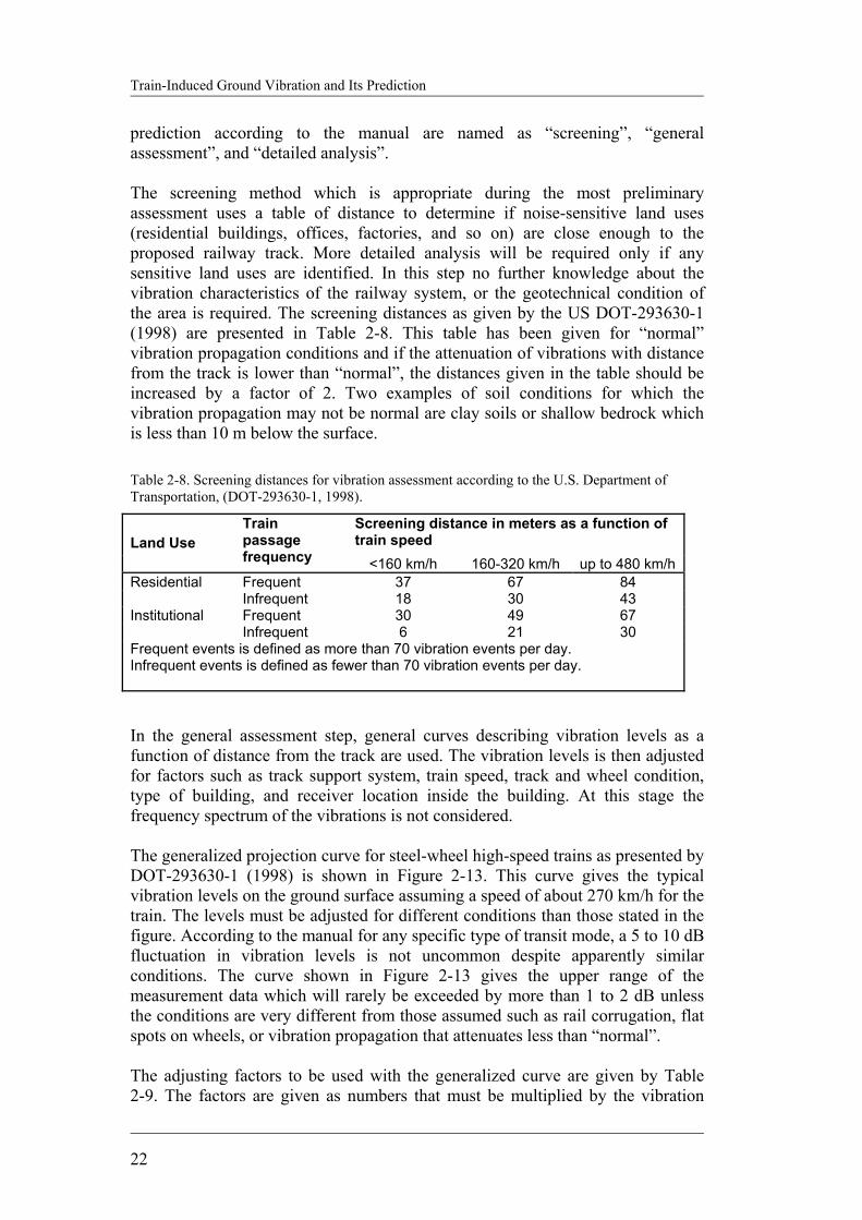
prediction according to the manual are named as “screening”, “general assessment”, and “detailed analysis”. The screening method which is appropriate during the most preliminary assessment uses a table of distance to determine if noise-sensitive land uses (residential buildings, offices, factories, and so on) are close enough to the proposed railway track. More detailed analysis will be required only if any sensitive land uses are identified. In this step no further knowledge about the vibration characteristics of the railway system, or the geotechnical condition of the area is required. The screening distances as given by the US DOT-293630-1 (1998) are presented in Table 2-8. This table has been given for “normal” vibration propagation conditions and if the attenuation of vibrations with distance from the track is lower than “normal”, the distances given in the table should be increased by a factor of 2. Two examples of soil conditions for which the vibration propagation may not be normal are clay soils or shallow bedrock which is less than 10 m below the surface. Table 2-8. Screening distances for vibration assessment according to the U.S. Department of Transportation, (DOT-293630-1, 1998).
Screening distance in meters as a function of train speed Land Use
Train passage frequency <160 km/h 160-320 km/h up to 480 km/h Frequent 37 67 84 Residential Infrequent 18 30 43 Frequent 30 49 67 Institutional Infrequent 6 21 30
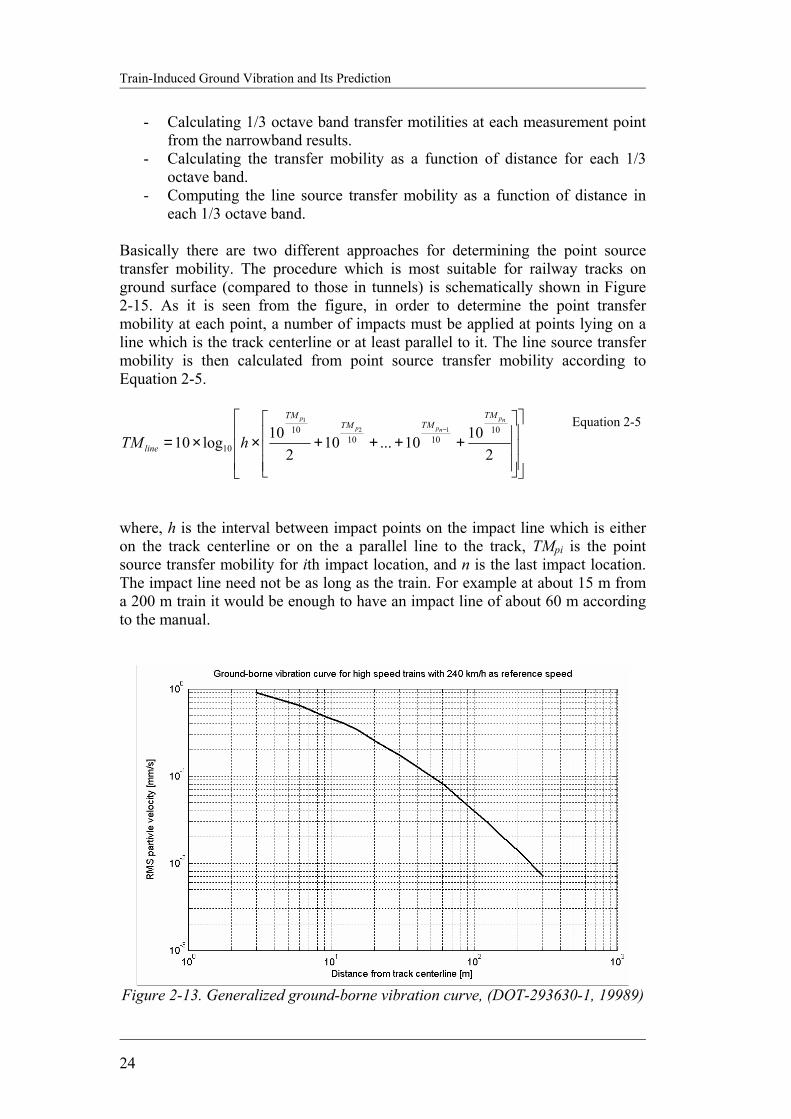
Frequent events is defined as more than 70 vibration events per day. Infrequent events is defined as fewer than 70 vibration events per day. In the general assessment step, general curves describing vibration levels as a function of distance from the track are used. The vibration levels is then adjusted for factors such as track support system, train speed, track and wheel condition, type of building, and receiver location inside the building. At this stage the frequency spectrum of the vibrations is not considered. The generalized projection curve for steel-wheel high-speed trains as presented by DOT-293630-1 (1998) is shown in Figure 2-13. This curve gives the typical vibration levels on the ground surface assuming a speed of about 270 km/h for the train. The levels must be adjusted for different conditions than those stated in the figure. According to the manual for any specific type of transit mode, a 5 to 10 dB fluctuation in vibration levels is not uncommon despite apparently similar conditions. The curve shown in Figure 2-13 gives the upper range of the measurement data which will rarely be exceeded by more than 1 to 2 dB unless the conditions are very different from those assumed such as rail corrugation, flat spots on wheels, or vibration propagation that attenuates less than “normal”. The adjusting factors to be used with the generalized curve are given by Table 2-9. The factors are given as numbers that must be multiplied by the vibration

Mehdi Bahrekazemi
23
value read from the curve shown in Figure 2-13. In using the adjustment factors for wheel and rail, only the largest adjustment factor is used and these two factors are not applied cumulatively. In the detailed analysis step, the vibrations at the specific site are predicted using the most accurate tools available. No standardized method has been developed for this level of analysis which is usually a complex procedure. There is not a clear distinction between the general and detailed analysis model. While some site measurements may be used for determining the generalized propagation curves (which may be considered as detailed analysis method), the generalized prediction curves may be sufficient for making ground vibration predictions in most cases except for special buildings. A detailed assessment is for example appropriate to examine areas where the general assessment phase indicated to have potential for high vibration impact. A site-specific model for detailed estimation of ground-borne vibration is suggested by DOT-293630-1, (1998). According to this manual the method provides “reasonable” estimate of vibration propagation characteristic of the site and that it can identify areas where ground-borne vibration will be higher than “normal”. The main idea of this procedure is to determine the experimental transfer mobility function for the specific site and then using the force density function obtained for the same kind of train at another site, predict the particle velocity at the new site. In doing so it is assumed that the force density function determined from measurements at a certain site for the type of the train is independent from the geological conditions of the site. In fact the force density function is not independent of the geological conditions of the site. Therefore using the force density function obtained from one site in calculations for other sites involves a rough approximation unless the two sites have similar geotechnical conditions. The r.m.s. vibration velocity level in 1/3 octave band according to this method is give by Equation 2-4.
buildlineFv CTMLL ++= Equation 2-4
where, Lv is the r.m.s. vibration velocity level in 1/3 octave band, LF is the force density for line vibration source, TMline is the line source transfer mobility from the track to a point on the ground close to the building, and Cbuild is the adjustment to account for ground-building foundation interaction and attenuation of vibration amplitudes as vibration propagates through the building. In order to determine the line source transfer mobility that probably is the most crucial part of this method, four steps as schematically shown in Figure 2-14 must be followed. These for steps are:
- Analyzing the field data to generate narrowband point source transfer mobilities.
Train-Induced Ground Vibration and Its Prediction
24
- Calculating 1/3 octave band transfer motilities at each measurement point from the narrowband results.
- Calculating the transfer mobility as a function of distance for each 1/3 octave band.
- Computing the line source transfer mobility as a function of distance in each 1/3 octave band.
Basically there are two different approaches for determining the point source transfer mobility. The procedure which is most suitable for railway tracks on ground surface (compared to those in tunnels) is schematically shown in Figure 2-15. As it is seen from the figure, in order to determine the point transfer mobility at each point, a number of impacts must be applied at points lying on a line which is the track centerline or at least parallel to it. The line source transfer mobility is then calculated from point source transfer mobility according to Equation 2-5.
++++××=
−
21010...10
210log10
101010
10
10
121 np
nppp TM
TMTMTM
line hTM
Equation 2-5
where, h is the interval between impact points on the impact line which is either on the track centerline or on the a parallel line to the track, TMpi is the point source transfer mobility for ith impact location, and n is the last impact location. The impact line need not be as long as the train. For example at about 15 m from a 200 m train it would be enough to have an impact line of about 60 m according to the manual.
Figure 2-13. Generalized ground-borne vibration curve, (DOT-293630-1, 19989)

Mehdi Bahrekazemi
25
Table 2-9. Adjustment factors due to vibration source to be used together with generalized curve shown in Figure 2-13, based on DOT-293630-1, (1998).
Factors Affecting Vibration Source
Source Factor Adjustment to Propagation curve Comment
Vehicle Speed (km/h)
Adjust. Factor
480 2.00 320 1.33 240 1.00 160 0.67
Speed
120 0.50
Vibration level in dB is proportional to 20.log(speed/speedref). Sometimes the vibration with speed has been observed to be as low as 10 to 15.log(speed/speedref). These adjustment factors should be multiplied by the base r.m.s. vibration read from Figure 2-13.
Resilient Wheels 1.00 Resilient wheels do not generally affect ground-borne vibration except at frequencies greater than 80 Hz.
Worn Wheels or Wheels with Flats 3.16
Wheel flats or wheels that are unevenly worn can cause high vibration levels. This problem can be prevented by wheel truing and slip-slide detectors to prevent the wheels from sliding on the track.
Worn or Corrugated Crack 3.16
If both the wheels and the track are worn, only one adjustment should be used. Corrugated track is a common problem, however it is difficult to predict the conditions that corrugations to occur. Rail grinding can remove rail corrugations.
Crossovers and Other Special
Track work 3.16
Wheel impacts at special track work with standard frogs will significantly increase vibration levels. This increase will be less at greater distances from the track. Moreover point frogs mitigate this problem.
Floating Slab Track bed. 0.18
The reduction achieved with a floating slab track bed is strongly dependent on the frequency characteristics of the vibration.
Ballast Mats 0.32 Actual reduction is strongly dependent on frequency of vibration.
High Resilience Fasteners 0.56
Slab track with fasteners that are very compliant in the vertical direction can reduce vibration at frequencies greater than 40 Hz.
Resiliently Supported Ties
Select highest one that applies
0.32 Resiliently supported tie system in tunnel have been found to provide very effective control of low-frequency vibration.
Relative to at-grade tie & ballast:
Ariel/ Viaduct
structure 0.32
Open Cut 1.00
Relative to bored tunnel in soil:
Station 0.56 Cut & Cover 0.71
Type of Track Structure
Rock-based 0.18
The general rule is the heavier the structure, the lower the vibration levels. Putting the track in cut may reduce the vibration levels slightly. Rock-based tunnels will shift vibration to a higher frequency.
Train-Induced Ground Vibration and Its Prediction
26
Table 2-10. Adjustment factors due to vibration path to be used together with generalized curve shown in Figure 2-13, based on DOT-293630-1, (1998).
Factors Affecting Vibration Path
Path Factor Adjustment to Propagation curve Comment
Efficient propagation in soil
3.16 Refer to DOT-293630-1 text for identifying areas where efficient propagation is possible.
Dist. (m)
Adjustment
15 1.26
30 1.58
45 2.00
Geological conditions that
promote effective vibration
propagation
Propagation
in Rock layer
60 2.82
The positive adjustment accounts for lower attenuation of vibration in rock compared to soil. Because it is more
difficult to get vibration energy into rock, propagation through rock usually results
in lower vibration than propagation through soil.
Wood Frame 0.56 1-2 Story
Commercial 0.45
2-4 story Masonry 0.32
Large Masonry on
piles 0.32
Large Masonry on
Spread Footings
0.22
Coupling to Building
Foundation
Foundation in Rock 1.00
The general rule is the heavier the building construction, the greater the coupling loss.
Table 2-11. Adjustment factors due to receiver to be used together with generalized curve shown
in Figure 2-13, based on DOT-293630-1, (1998).
Factors Affecting Vibration Receiver Receiver Factor
Adjustment to Propagation curve Comment
1 to 5 floors above grade 0.80
Floor-to-Floor Attenuation 5 to 10 floors above
grade 0.90
This factor accounts for dispersion and attenuation of the vibration energy as it propagates through a building.
Amplification due to Resonances of Floors, Walls, and Ceilings
2.00
The actual amplification will vary greatly depending on the type of construction. The amplification is lower near the wall-floor and wall-ceiling intersections.
Mehdi Bahrekazemi
27
After establishing the line source transfer mobility for the site, the force density can be determined using Equation 2-6.
linevF TMLL −= Equation 2-6
where, LF is the force density, Lv is measured ground vibration during passage of a certain type train, and TMline is the line source transfer mobility. In order to develop force density for a certain type of train, the procedure is repeated at three
Figure 2-15. Schematic plan for transfer mobility measurements (DOT-293630-1, 1998).
Figure 2-14. Process of calculating the transfer mobility according to DOT-293630-1,
(1998).
Train-Induced Ground Vibration and Its Prediction
28
or more positions and force density is declared as the average of LF obtained for these positions. It seems that the force density obtained in this way is only applicable to places where a similar type of embankment is planed. This is due to the fact that vibration measurements for the same type of train on two different embankments may result in different vibration levels running at almost the same speed. A simple method has been suggested by the manual for considering the train speed. Equation 2-7 that is similar to the one suggested by Madshus et al. (1996), gives the needed adjustment for the train speed. The estimated ground vibration must then be adjusted for building response, coupling loss, and transmission through the building.
)log(20)(refvvVdBadjustment ×=
Equation 2-7
Where, vref is the speed of the train that has been used in development of the model, and v represents the design speed of the train for the new track. While the equation provides a simple way of accounting for the train speed factor, it does not consider phenomena like running the train at speeds close to the critical speed of the track.
2.4.3 Norwegian model A semi-empirical model for predicting low frequency vibrations from railway traffic on soft soils has been developed by Norwegian Geotechnical Institue, NGI (Madshus et al., 1996). The model which has a statistical formulation predicts both expected values and the corresponding confidence limits. This model has been used in planning Gardemobanen (high-speed railway track between Oslo and the airport). The model predicts vibration at mid-floor spans of the buildings that are situated at a distance from the track. Data used for this prediction model have been collected from measurements at different sites with soil conditions varying from soft to stiff soil and various building types. The sites are located along different railway lines in Norway and Sweden. The vibrations have been measured simultaneously on the embankment, at several points on the ground surface, on building foundations, and on higher stories of the buildings. The frequency domain for the stored data from the measurements cover at least the frequencies between 3 and 80 Hz. Considering the stochastic nature of railway related ground vibrations, usually more than five to ten passages of the same train type have been recorded. Based on recorded time histories, one-third octave values and frequency weighted r.m.s. values according to ISO 2631 and ISO 8041, with a one second integration time for the most intense part of the recordings have been evaluated. The factors that are recognized by NGI to be important for the model are:
• Ground conditions
Mehdi Bahrekazemi
29
• Train type • Line quality and embankment design • Train speed • Distance from the track to the building • Building foundation, structure, and number of floors
In an attempt to simplify the model it has been assumed that the effects of factors 2-6 can be considered separately. Combining some of the factors named above, the model is given in mathematical form as in Equation 2-8.
[ ] BRDsTBRv FFFFVFFFV == Equation 2-8
Here Fv is the basic vibration function, FR is the track quality factor, and FB is the building amplification factor. The basic vibration factor is in its turn comprised of three other factors. These factors are VT which is a train type specific vibration level, defined as the vibration level on the ground at a reference distance of D0=15m, from the centerline of the track, when a train of a certain type passes at a reference speed of S0=70 km/h, on a “Standard” track and embankment. The reference distance, 15m from the centerline of the track has been chosen so that the influence of the near field waves could be avoided. FS is a speed factor that accounts for the train speed S. This factor is defined in Equation 2-9, in which A is the train speed factor.
A
S SSF
=
0
Equation 2-9
Similar to FS , FD is distance factor, which accounts for the attenuation with distance from the track, due to both geometrical and hysteretic damping. FD is defined according to Equation 2-10, where D is the distance from the midpoint of the track to the receiver, and B is the distance exponent.
B
D DDF
−
=
0
Equation 2-10
While the factor VT and the distance exponent B both depend on the ground conditions, the speed exponent A is reported not to vary significantly with the ground conditions and is reported to be about one. The track quality factor, FR takes into account the effect of the track quality and the embankment on the vibrations. A massive and stiff embankment under the rails is expected to give less vibration than the “standard” track, while a too flexible embankment would result in more vibrations than the “standard” track. This factor even takes into account the smoothness of the rails. Finally FB, the building amplification factor takes into account the effect of the ground/foundation coupling and building resonances on the vibrations measured
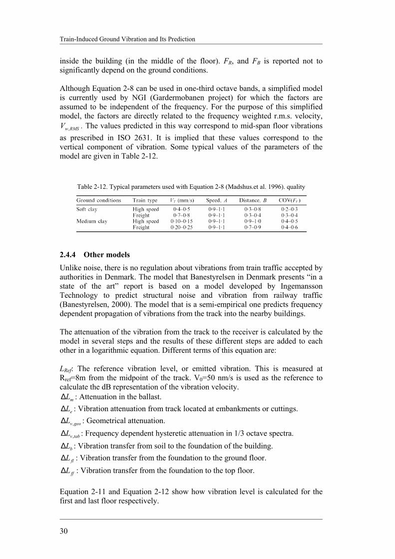
Train-Induced Ground Vibration and Its Prediction
30
inside the building (in the middle of the floor). FR, and FB is reported not to significantly depend on the ground conditions. Although Equation 2-8 can be used in one-third octave bands, a simplified model is currently used by NGI (Gardermobanen project) for which the factors are assumed to be independent of the frequency. For the purpose of this simplified model, the factors are directly related to the frequency weighted r.m.s. velocity,
RMSwV , . The values predicted in this way correspond to mid-span floor vibrations as prescribed in ISO 2631. It is implied that these values correspond to the vertical component of vibration. Some typical values of the parameters of the model are given in Table 2-12.
Table 2-12. Typical parameters used with Equation 2-8 (Madshus.et al. 1996). quality
2.4.4 Other models Unlike noise, there is no regulation about vibrations from train traffic accepted by authorities in Denmark. The model that Banestyrelsen in Denmark presents “in a state of the art” report is based on a model developed by Ingemansson Technology to predict structural noise and vibration from railway traffic (Banestyrelsen, 2000). The model that is a semi-empirical one predicts frequency dependent propagation of vibrations from the track into the nearby buildings. The attenuation of the vibration from the track to the receiver is calculated by the model in several steps and the results of these different steps are added to each other in a logarithmic equation. Different terms of this equation are: LRef: The reference vibration level, or emitted vibration. This is measured at Rref=8m from the midpoint of the track. V0=50 nm/s is used as the reference to calculate the dB representation of the vibration velocity.
mL∆ : Attenuation in the ballast.
eL∆ : Vibration attenuation from track located at embankments or cuttings.
geovL ,∆ : Geometrical attenuation.
tabvL ,∆ : Frequency dependent hysteretic attenuation in 1/3 octave spectra.
bL∆ : Vibration transfer from soil to the foundation of the building.
flL∆ : Vibration transfer from the foundation to the ground floor.
ffL∆ : Vibration transfer from the foundation to the top floor. Equation 2-11 and Equation 2-12 show how vibration level is calculated for the first and last floor respectively.
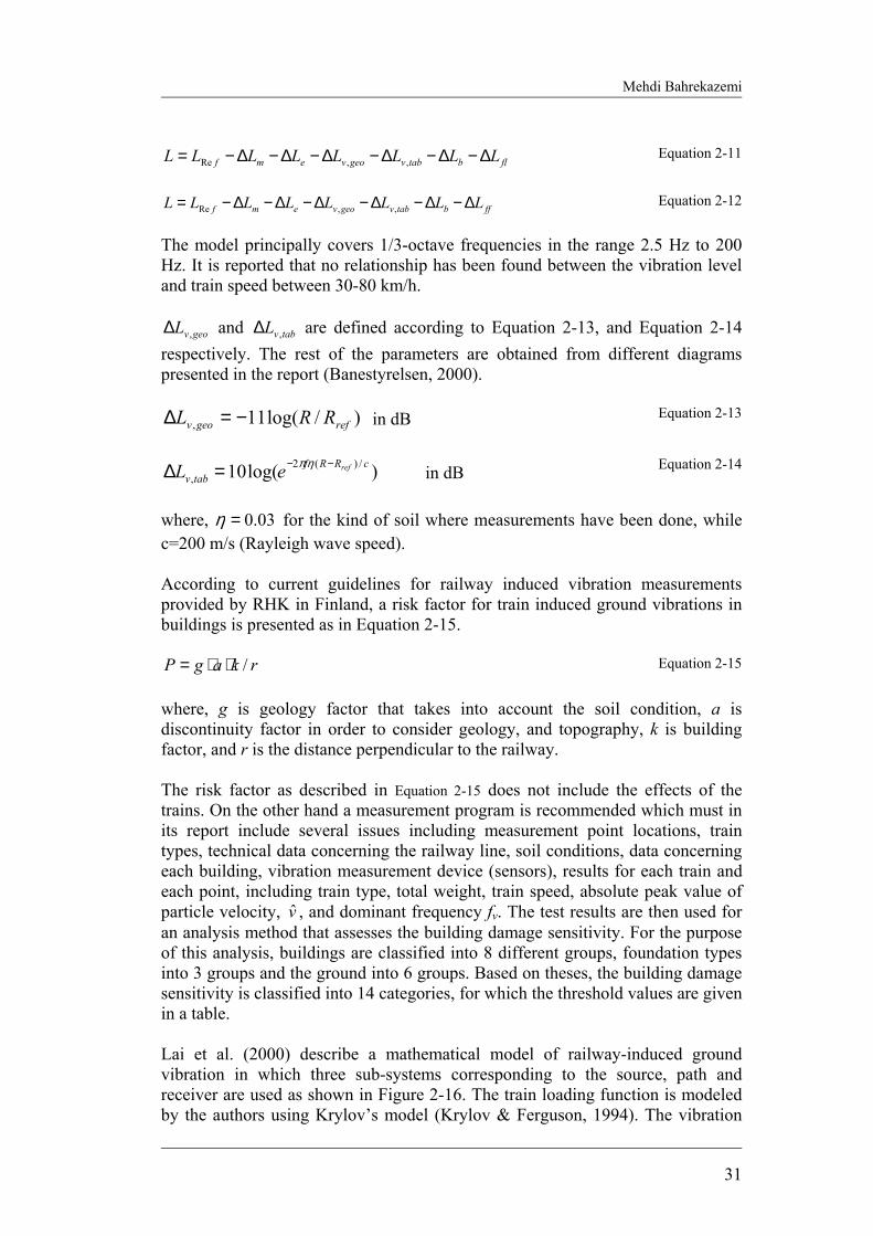
Mehdi Bahrekazemi
31
flbtabvgeovemf LLLLLLLL ∆−∆−∆−∆−∆−∆−= ,,Re Equation 2-11
ffbtabvgeovemf LLLLLLLL ∆−∆−∆−∆−∆−∆−= ,,Re Equation 2-12
The model principally covers 1/3-octave frequencies in the range 2.5 Hz to 200 Hz. It is reported that no relationship has been found between the vibration level and train speed between 30-80 km/h.
geovL ,∆ and tabvL ,∆ are defined according to Equation 2-13, and Equation 2-14 respectively. The rest of the parameters are obtained from different diagrams presented in the report (Banestyrelsen, 2000).
)/log(11, refgeov RRL −=∆ in dB Equation 2-13
)log(10 /)(2
,cRRf
tabvrefeL −−=∆ ηπ in dB Equation 2-14
where, 03.0=η for the kind of soil where measurements have been done, while c=200 m/s (Rayleigh wave speed). According to current guidelines for railway induced vibration measurements provided by RHK in Finland, a risk factor for train induced ground vibrations in buildings is presented as in Equation 2-15.
rkagP /⋅⋅= Equation 2-15
where, g is geology factor that takes into account the soil condition, a is discontinuity factor in order to consider geology, and topography, k is building factor, and r is the distance perpendicular to the railway. The risk factor as described in Equation 2-15 does not include the effects of the trains. On the other hand a measurement program is recommended which must in its report include several issues including measurement point locations, train types, technical data concerning the railway line, soil conditions, data concerning each building, vibration measurement device (sensors), results for each train and each point, including train type, total weight, train speed, absolute peak value of particle velocity, v , and dominant frequency fv. The test results are then used for an analysis method that assesses the building damage sensitivity. For the purpose of this analysis, buildings are classified into 8 different groups, foundation types into 3 groups and the ground into 6 groups. Based on theses, the building damage sensitivity is classified into 14 categories, for which the threshold values are given in a table. Lai et al. (2000) describe a mathematical model of railway-induced ground vibration in which three sub-systems corresponding to the source, path and receiver are used as shown in Figure 2-16. The train loading function is modeled by the authors using Krylov’s model (Krylov & Ferguson, 1994). The vibration
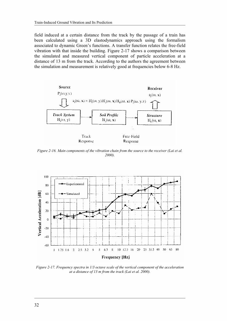
Train-Induced Ground Vibration and Its Prediction
32
field induced at a certain distance from the track by the passage of a train has been calculated using a 3D elastodynamics approach using the formalism associated to dynamic Green’s functions. A transfer function relates the free-field vibration with that inside the building. Figure 2-17 shows a comparison between the simulated and measured vertical component of particle acceleration at a distance of 13 m from the track. According to the authors the agreement between the simulation and measurement is relatively good at frequencies below 6-8 Hz.
Figure 2-16. Main components of the vibration chain from the source to the receiver (Lai et al.
2000).
Figure 2-17. Frequency spectra in 1/3 octave scale of the vertical component of the acceleration
at a distance of 13 m from the track (Lai et al. 2000).
Mehdi Bahrekazemi
33
2.5 DISCUSSION AND CONCLUSIONS The problem of excessive ground vibration has three main components. These components or links are the source, the propagation path and the receiver. Therefore in order to study the issue of ground-borne vibration all the three links should be considered. Ground-borne vibration caused by train traffic is influenced by factors as wheel and rail roughness, dynamic characteristics of the rolling stock, train speed, discrete track supports, rail support stiffness, railway structure design, soil characteristics, and building structure design. The most important effect of ground-borne vibration caused by train traffic is on the human occupants. If there is vibration sensitive equipment inside the building its function may be disrupted by the vibration if countermeasures are not taken. Usually there are no damage impacts on the building or even its cosmetic parts due to train-induced ground vibration. Nevertheless in case of old historical buildings that are situated very close to the railway track the issue should be considered in more detail. Mitigation methods are available to be used with each of the three links discussed above. What method or combination of methods should be used depends on factors as, what the frequency content of the generated ground-borne vibration is, how far the building is from the track, what is the type and layering of the soil at the site, how many buildings must be protected from excessive ground-borne vibration, and what are the types of the buildings. Ground-borne vibration in combination with noise from railway may be perceived by people as more annoying. Therefore it is recommendable to combine noise and vibration mitigation methods to achieve the best results. Three different model classes may be identified for prediction of ground-borne vibration due to train traffic. The first class (class I) includes scoping models that should be used at the earliest phase of the project to primarily identify those parts along the track that may have excessive ground-borne vibration. The second class (class II) includes those models that are more accurate than class I and are suitable for the purpose of quantifying the severity of the problem more precisely. Finally, those models that have the best accuracy and can be used to support the design and specification of the track and possible mitigation measures are classified as class III. Class III models, despite being the most accurate models, are very time consuming and usually need special site measurements to be performed in order to determine the needed parameters of the model. This makes these models appropriate for use only in the last phase of the design in order to avoid unnecessary costs. Therefore class I and class II models are needed for studying large areas in order to identify places where there is risk for excessive ground-borne vibration. On the other hand the accuracy of the available models is not good and there is need for developing more accurate models that at the same time are easy to use.

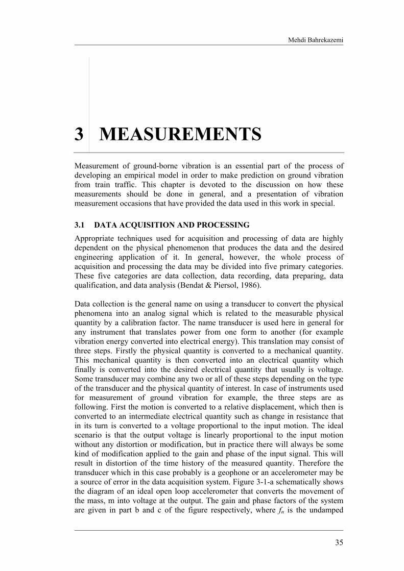
Mehdi Bahrekazemi
35
3 MEASUREMENTS Measurement of ground-borne vibration is an essential part of the process of developing an empirical model in order to make prediction on ground vibration from train traffic. This chapter is devoted to the discussion on how these measurements should be done in general, and a presentation of vibration measurement occasions that have provided the data used in this work in special.
3.1 DATA ACQUISITION AND PROCESSING Appropriate techniques used for acquisition and processing of data are highly dependent on the physical phenomenon that produces the data and the desired engineering application of it. In general, however, the whole process of acquisition and processing the data may be divided into five primary categories. These five categories are data collection, data recording, data preparing, data qualification, and data analysis (Bendat & Piersol, 1986). Data collection is the general name on using a transducer to convert the physical phenomena into an analog signal which is related to the measurable physical quantity by a calibration factor. The name transducer is used here in general for any instrument that translates power from one form to another (for example vibration energy converted into electrical energy). This translation may consist of three steps. Firstly the physical quantity is converted to a mechanical quantity. This mechanical quantity is then converted into an electrical quantity which finally is converted into the desired electrical quantity that usually is voltage. Some transducer may combine any two or all of these steps depending on the type of the transducer and the physical quantity of interest. In case of instruments used for measurement of ground vibration for example, the three steps are as following. First the motion is converted to a relative displacement, which then is converted to an intermediate electrical quantity such as change in resistance that in its turn is converted to a voltage proportional to the input motion. The ideal scenario is that the output voltage is linearly proportional to the input motion without any distortion or modification, but in practice there will always be some kind of modification applied to the gain and phase of the input signal. This will result in distortion of the time history of the measured quantity. Therefore the transducer which in this case probably is a geophone or an accelerometer may be a source of error in the data acquisition system. Figure 3-1-a schematically shows the diagram of an ideal open loop accelerometer that converts the movement of the mass, m into voltage at the output. The gain and phase factors of the system are given in part b and c of the figure respectively, where fn is the undamped

Train-Induced Ground Vibration and Its Prediction
36
natural frequency and ζ is the damping ratio of the system. It is seen from the figure that if for example ζ =0.7, the signal measured at the output is flat in magnitude up to about 50 % of the undamped natural frequency of the accelerometer and the phase angle will be distorted by about 40° at this frequency (0.5fn). Therefore the type of accelerometer used for measurements should have an undamped natural frequency considerably higher than the highest frequency of interest in the signal. In case of geophones the corresponding response curve for the magnitude will be flat for frequencies higher than about two times the undamped natural frequency of the geophone as shown by Figure 3-5 for a certain type of geophone.
Figure 3-1. Schematic diagram and response characteristic of open loop seismic accelerometer.
(a) Schematic diagram of idealized accelerometer. (b)Accelerometer gain factor. (c)Accelerometer phase factor (Bendat & Piersol, 1986).
After collecting the data by the transducer, the signal is conditioned if necessary and then recorded either by some kind of tape recorder or directly on the hard disc of a computer. Figure 3-2 shows schematically the usual data acquisition system for the measurements carried out by KTH that are presented here. As it is seen from the figure the signal from strain gauges and accelerometers are first amplified before going to the DAT tape recorder for recording at the chosen sampling frequency. Geophone signals on the other hand are recorded directly. The DAT tape recorder can record the signals at sampling frequencies up to 12 kHz. Usually a sampling frequency of 6 kHz has been used for this purpose. Later in the laboratory the data is down loaded from the tapes and saved on CD for further analysis. The data may be down sampled to the required sampling frequency for the purpose of analysis. The DAT tape recorder used for the

Mehdi Bahrekazemi
37
measurements can receive up to 16 channels corresponding to 16 different sensors. If the number of channels is more than 16, two recorders may be used with at least one common channel that can be used for synchronization. At some occasions the collected data is directly recorded on the hard disc using a special data acquisition system as described in section 3.2.2.2. The preparation of data for analysis includes conversion of data from analog to digital which nowadays is performed during data collection phase and editing the data and removing the spurious and corrupt data signals. The last part is usually performed visually by an experienced person.
D
ADAT recorder for
recording the signals atcertain sampling frequency
(example 6 kHz) Computer formonitoring the signals
Geoph.Acc.Straingauge
Amplifier Amplifier
Figure 3-2. Data acquisition system used for the measurements.
The next step is data qualification. In this step the data is tested to recognized basic characteristics of the data. Being stationary or not, presence of periodicity, and normality of the data are the three most important issues that may be considered in this step. In practice however this step is an integral part of data analysis. Finally the data is analyzed using appropriate methods to determine for example the mean value and mean square value of the data, and its frequency spectrum.
3.1.1 Measurement equipment used for KTH measurements In this section all the sensors that have been used for the measurements in the framework of the two projects FreightVib and Envib are presented. The quantities that have been measured during these measurement occasions are ground vibration, either particle acceleration or particle velocity, and wheel force.

Train-Induced Ground Vibration and Its Prediction
38
Wheel force is one of the most important parameters with respect to train induced-ground vibration. One of the methods to measure wheel force as schematically shown in Figure 3-3, is using strain gauges to measure the changes in shear stress of the rail during passage of the train wheels. In order to determine the wheel force, the strain gauges are calibrated using a known load like that from the hydraulic jack of TLV, Banverket’s measuring car as shown in Figure 3-14. After removing the rust from the surface of the steel the four strain gauges (two on each side of the rail web) are glued to the rail using for example X60 glue. The location of the strain gauge is on the neutral line of the rail, and a few centimeters from the sleepers as shown in Figure 3-3 and Figure 3-4. There are two rosettes in each strain gauge which must be placed at 45 degrees to the neutral line. Theoretically it is enough to have the strain gauges only on one side of the rail web, but in practice usually four strain gauges are used (two on each side) thereby measuring the average of shear strain on both sides of the rail. When the glue is hardened the strain gauges are covered by a water proof layer. Figure 3-4 shows the strain gauges used for KTH measurements being attached to the web of the rail according to this procedure.
~150 mm
UIC
60:
81 m
m
C
D
A
B A'
B'
C'
D'
AB & CD A'B'& C'D'
A
A'
B B'
C
D
C'
D'
d
c b
a
cd ab
Figure 3-3. Schematic figure showing how the strain gauges can be connected to each other in
order to measure the shear force in the rail.
Figure 3-4. Mounting strain gauges on the web of the rail in order to measure wheel force.
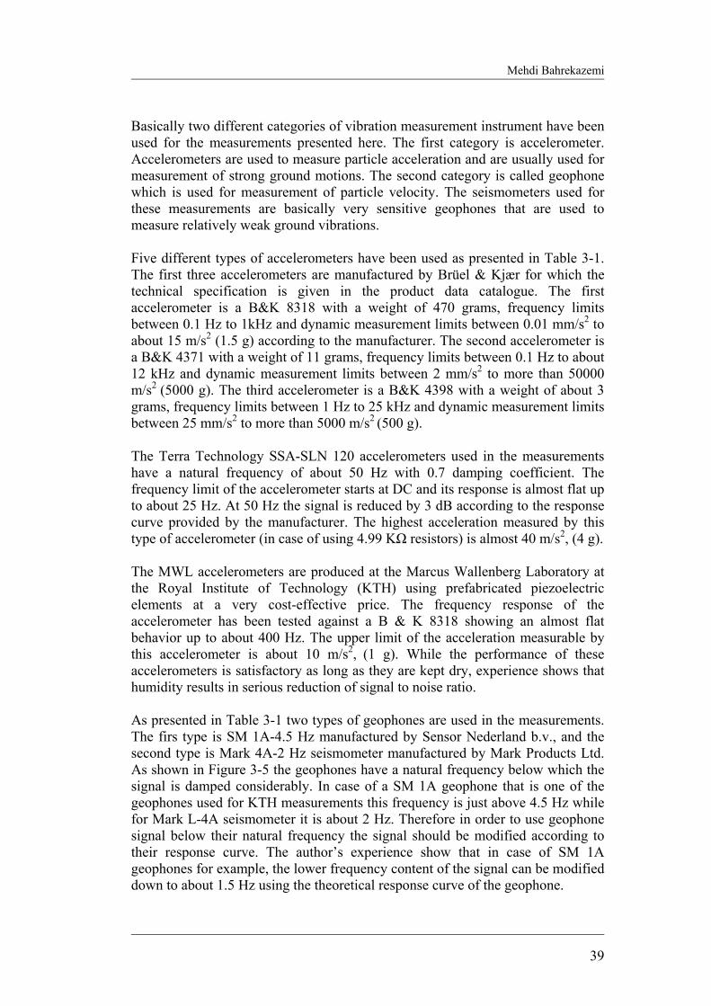
Mehdi Bahrekazemi
39
Basically two different categories of vibration measurement instrument have been used for the measurements presented here. The first category is accelerometer. Accelerometers are used to measure particle acceleration and are usually used for measurement of strong ground motions. The second category is called geophone which is used for measurement of particle velocity. The seismometers used for these measurements are basically very sensitive geophones that are used to measure relatively weak ground vibrations. Five different types of accelerometers have been used as presented in Table 3-1. The first three accelerometers are manufactured by Brüel & Kjær for which the technical specification is given in the product data catalogue. The first accelerometer is a B&K 8318 with a weight of 470 grams, frequency limits between 0.1 Hz to 1kHz and dynamic measurement limits between 0.01 mm/s2 to about 15 m/s2 (1.5 g) according to the manufacturer. The second accelerometer is a B&K 4371 with a weight of 11 grams, frequency limits between 0.1 Hz to about 12 kHz and dynamic measurement limits between 2 mm/s2 to more than 50000 m/s2 (5000 g). The third accelerometer is a B&K 4398 with a weight of about 3 grams, frequency limits between 1 Hz to 25 kHz and dynamic measurement limits between 25 mm/s2 to more than 5000 m/s2 (500 g). The Terra Technology SSA-SLN 120 accelerometers used in the measurements have a natural frequency of about 50 Hz with 0.7 damping coefficient. The frequency limit of the accelerometer starts at DC and its response is almost flat up to about 25 Hz. At 50 Hz the signal is reduced by 3 dB according to the response curve provided by the manufacturer. The highest acceleration measured by this type of accelerometer (in case of using 4.99 KΩ resistors) is almost 40 m/s2, (4 g). The MWL accelerometers are produced at the Marcus Wallenberg Laboratory at the Royal Institute of Technology (KTH) using prefabricated piezoelectric elements at a very cost-effective price. The frequency response of the accelerometer has been tested against a B & K 8318 showing an almost flat behavior up to about 400 Hz. The upper limit of the acceleration measurable by this accelerometer is about 10 m/s2, (1 g). While the performance of these accelerometers is satisfactory as long as they are kept dry, experience shows that humidity results in serious reduction of signal to noise ratio. As presented in Table 3-1 two types of geophones are used in the measurements. The firs type is SM 1A-4.5 Hz manufactured by Sensor Nederland b.v., and the second type is Mark 4A-2 Hz seismometer manufactured by Mark Products Ltd. As shown in Figure 3-5 the geophones have a natural frequency below which the signal is damped considerably. In case of a SM 1A geophone that is one of the geophones used for KTH measurements this frequency is just above 4.5 Hz while for Mark L-4A seismometer it is about 2 Hz. Therefore in order to use geophone signal below their natural frequency the signal should be modified according to their response curve. The author’s experience show that in case of SM 1A geophones for example, the lower frequency content of the signal can be modified down to about 1.5 Hz using the theoretical response curve of the geophone.
Train-Induced Ground Vibration and Its Prediction
40
Figure 3-5. Theoretical response curve for the SM 1A-4.5 Hz geophones.
Both the accelerometers and geophones used for the measurements performed by KTH are calibrated using accelerometers that themselves have already been calibrated by SP Swedish National Testing and Research Institute. For calibrating the geophones for example, the geophone and the calibrated accelerometer are mounted on an electrical vibrator as shown in Figure 3-6. Then the vibrator is adjusted to vibrate at a known frequency and the signals from the geophone and accelerometer are read using a data acquisition system as shown in the left part of the figure. Knowing the acceleration, the velocity is determined from Equation 3-1, and thereby the calibration factor for the geophone is determined.
fwhere
AV
⋅⋅=
=
πω
ω
2
/
Equation 3-1
A summary of all sensors used for KTH measurements and their sensitivity is presented in Table 3-1. In the column for name of the sensor, a sign is also attributed to each sensor which is later used on the instrumentation plan of the measurements.
Figure 3-6. Calibration of SM 1A-4.5 Hz geophone using a calibrated accelerometer.
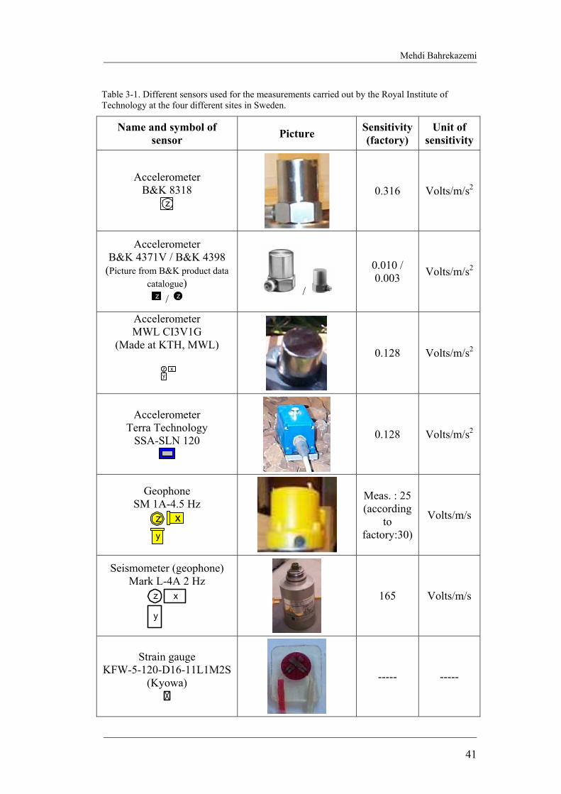
Mehdi Bahrekazemi
41
Table 3-1. Different sensors used for the measurements carried out by the Royal Institute of Technology at the four different sites in Sweden.
Name and symbol of sensor Picture Sensitivity
(factory) Unit of
sensitivity
Accelerometer B&K 8318
z
0.316 Volts/m/s2
Accelerometer B&K 4371V / B&K 4398
(Picture from B&K product data catalogue)
z / z /
0.010 / 0.003 Volts/m/s2
Accelerometer MWL CI3V1G
(Made at KTH, MWL)
yz x
0.128 Volts/m/s2
Accelerometer Terra Technology
SSA-SLN 120
0.128 Volts/m/s2
Geophone SM 1A-4.5 Hz
zy
x
Meas. : 25 (according
to factory:30)
Volts/m/s
Seismometer (geophone) Mark L-4A 2 Hz
x
y
z
165 Volts/m/s
Strain gauge KFW-5-120-D16-11L1M2S
(Kyowa)
----- -----
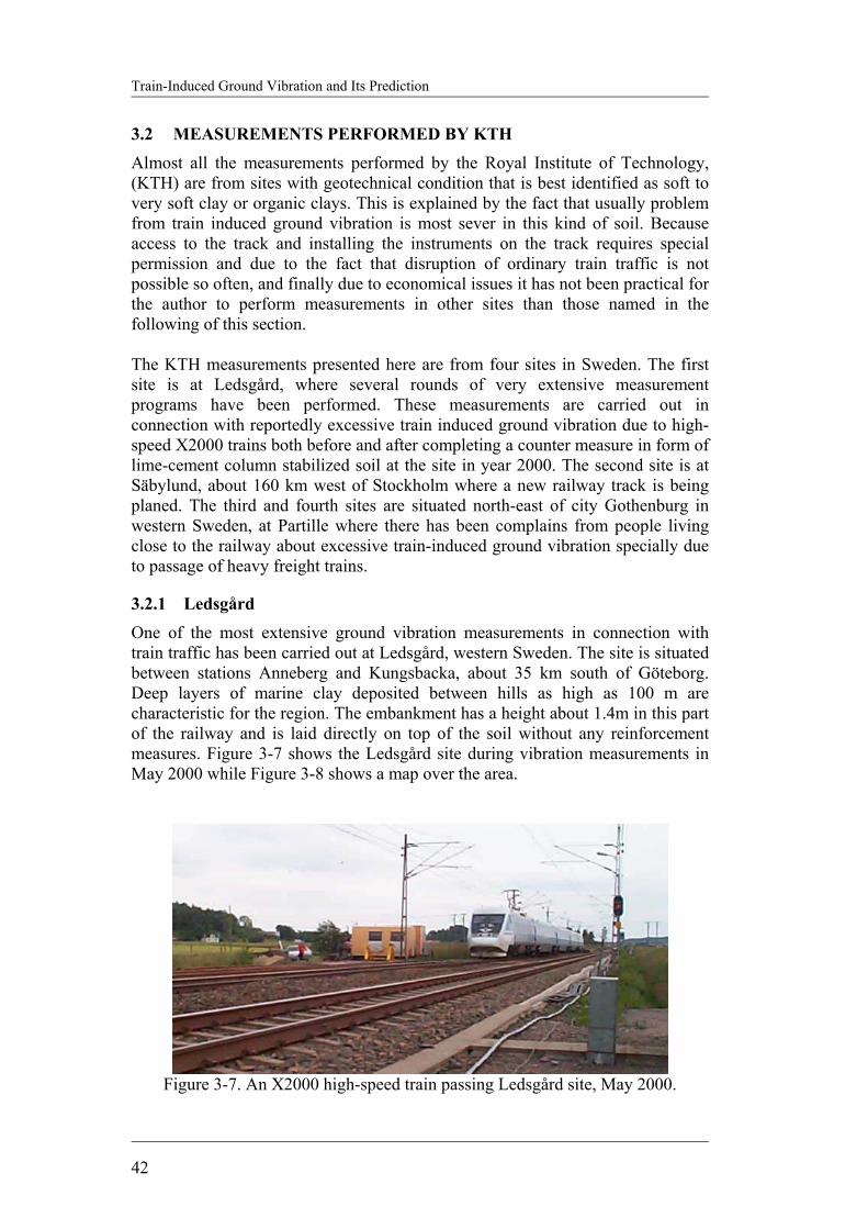
Train-Induced Ground Vibration and Its Prediction
42
3.2 MEASUREMENTS PERFORMED BY KTH Almost all the measurements performed by the Royal Institute of Technology, (KTH) are from sites with geotechnical condition that is best identified as soft to very soft clay or organic clays. This is explained by the fact that usually problem from train induced ground vibration is most sever in this kind of soil. Because access to the track and installing the instruments on the track requires special permission and due to the fact that disruption of ordinary train traffic is not possible so often, and finally due to economical issues it has not been practical for the author to perform measurements in other sites than those named in the following of this section. The KTH measurements presented here are from four sites in Sweden. The first site is at Ledsgård, where several rounds of very extensive measurement programs have been performed. These measurements are carried out in connection with reportedly excessive train induced ground vibration due to high-speed X2000 trains both before and after completing a counter measure in form of lime-cement column stabilized soil at the site in year 2000. The second site is at Säbylund, about 160 km west of Stockholm where a new railway track is being planed. The third and fourth sites are situated north-east of city Gothenburg in western Sweden, at Partille where there has been complains from people living close to the railway about excessive train-induced ground vibration specially due to passage of heavy freight trains.
3.2.1 Ledsgård One of the most extensive ground vibration measurements in connection with train traffic has been carried out at Ledsgård, western Sweden. The site is situated between stations Anneberg and Kungsbacka, about 35 km south of Göteborg. Deep layers of marine clay deposited between hills as high as 100 m are characteristic for the region. The embankment has a height about 1.4m in this part of the railway and is laid directly on top of the soil without any reinforcement measures. Figure 3-7 shows the Ledsgård site during vibration measurements in May 2000 while Figure 3-8 shows a map over the area.
Figure 3-7. An X2000 high-speed train passing Ledsgård site, May 2000.
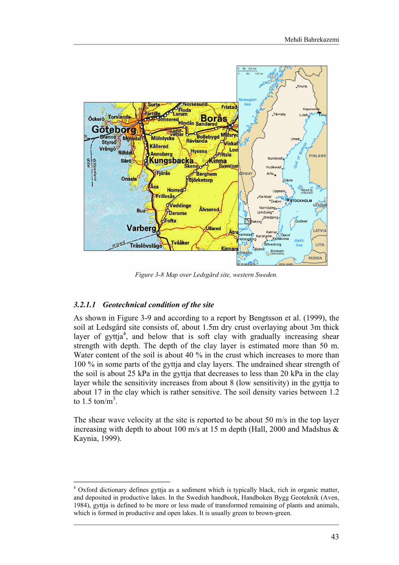
Mehdi Bahrekazemi
43
Figure 3-8 Map over Ledsgård site, western Sweden.
3.2.1.1 Geotechnical condition of the site As shown in Figure 3-9 and according to a report by Bengtsson et al. (1999), the soil at Ledsgård site consists of, about 1.5m dry crust overlaying about 3m thick layer of gyttja4, and below that is soft clay with gradually increasing shear strength with depth. The depth of the clay layer is estimated more than 50 m. Water content of the soil is about 40 % in the crust which increases to more than 100 % in some parts of the gyttja and clay layers. The undrained shear strength of the soil is about 25 kPa in the gyttja that decreases to less than 20 kPa in the clay layer while the sensitivity increases from about 8 (low sensitivity) in the gyttja to about 17 in the clay which is rather sensitive. The soil density varies between 1.2 to 1.5 ton/m3. The shear wave velocity at the site is reported to be about 50 m/s in the top layer increasing with depth to about 100 m/s at 15 m depth (Hall, 2000 and Madshus & Kaynia, 1999).
4 Oxford dictionary defines gyttja as a sediment which is typically black, rich in organic matter, and deposited in productive lakes. In the Swedish handbook, Handboken Bygg Geoteknik (Aven, 1984), gyttja is defined to be more or less made of transformed remaining of plants and animals, which is formed in productive and open lakes. It is usually green to brown-green.
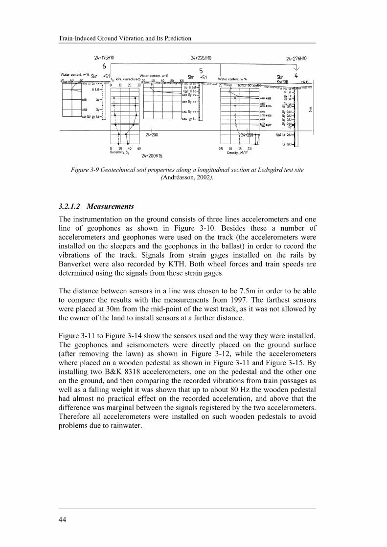
Train-Induced Ground Vibration and Its Prediction
44
Figure 3-9 Geotechnical soil properties along a longitudinal section at Ledsgård test site
(Andréasson, 2002).
3.2.1.2 Measurements The instrumentation on the ground consists of three lines accelerometers and one line of geophones as shown in Figure 3-10. Besides these a number of accelerometers and geophones were used on the track (the accelerometers were installed on the sleepers and the geophones in the ballast) in order to record the vibrations of the track. Signals from strain gages installed on the rails by Banverket were also recorded by KTH. Both wheel forces and train speeds are determined using the signals from these strain gages. The distance between sensors in a line was chosen to be 7.5m in order to be able to compare the results with the measurements from 1997. The farthest sensors were placed at 30m from the mid-point of the west track, as it was not allowed by the owner of the land to install sensors at a farther distance. Figure 3-11 to Figure 3-14 show the sensors used and the way they were installed. The geophones and seismometers were directly placed on the ground surface (after removing the lawn) as shown in Figure 3-12, while the accelerometers where placed on a wooden pedestal as shown in Figure 3-11 and Figure 3-15. By installing two B&K 8318 accelerometers, one on the pedestal and the other one on the ground, and then comparing the recorded vibrations from train passages as well as a falling weight it was shown that up to about 80 Hz the wooden pedestal had almost no practical effect on the recorded acceleration, and above that the difference was marginal between the signals registered by the two accelerometers. Therefore all accelerometers were installed on such wooden pedestals to avoid problems due to rainwater.

Mehdi Bahrekazemi
45
zx
y
z
y
xyz
x
z
y
x
z
x
y z
z
z
yz
z
z
x
43
2
87
6
z
z
z
z
z
z
z
z
z
5
1
7.5 m 7.5 m
7.5
m7.
5 m
7.5
m7.
5 m
~0.3 m
depth 0 & 5 m
Geoph. Mark L-4A Geoph. SM-1A 4.5Hz Acc. B&K 4371
Acc. MWL Acc. B&K 8318 Strain gauges
A B C
1
2
3
4
15,16,39,40
9 17
10
1112
13 24
14
yz x
20 23
222118
19
yz x
depth 0 & 3 m
yz x
27 30
292825
26
31
32
33
34
35
36
37
38
TT SSA-SLN 120
z
Figure 3-10. Instrumentation plan for vibration measurements, May 2000, Ledsgård, Sweden.

Train-Induced Ground Vibration and Its Prediction
46
Figure 3-11 One-axial MWL accelerometer mounted on a wooden pedestal in the ground.
Figure 3-12 Three MARK L-4A seismometers and a three-axial MWL accelerometer on the ground and a three-axial MWL accelerometer in 3 m depth (in the hole shown at the bottom of the figure).
Figure 3-13 Three-axial SM 1A-4.5 geophone installed in the ballast beside the rail.
Figure 3-14 Loading the rail by hydraulic jack of the TLV, Banverket’s measuring car.

Mehdi Bahrekazemi
47
Figure 3-15 Test performed with B&K 8318 accelerometer in order to study the effect of the pedestals. Two other rounds of vibration measurements in Oct. and Dec. 2000, involving passage of different trains were also carried out at Ledsgård. These measurements were performed after that lime-cement column soil stabilization was completed under the west track. For October as well as December measurements, the instrumentation on the ground consisted of one line accelerometers and one line geophones as shown in Figure 3-16. Besides these a number of accelerometers and geophones were used on the track (the accelerometers were installed on the sleepers) in order to record the vibration of the track. Signals from two strain gauges installed on the rails by Banverket were also recorded. The sensors were installed in the same way as in May. The signal from the TT SSA-SLN 120 accelerometer was recorded separately by Banverket in December which was later made available to KTH. The common channel between Banverket and KTH measurements was from the strain gauges. The data acquisition system for all measurement occasions at Ledsgård test site consists of a DAT tape recorder and a computer used for monitoring the signals similar to the one used at Partille that is shown in Figure 3-38.
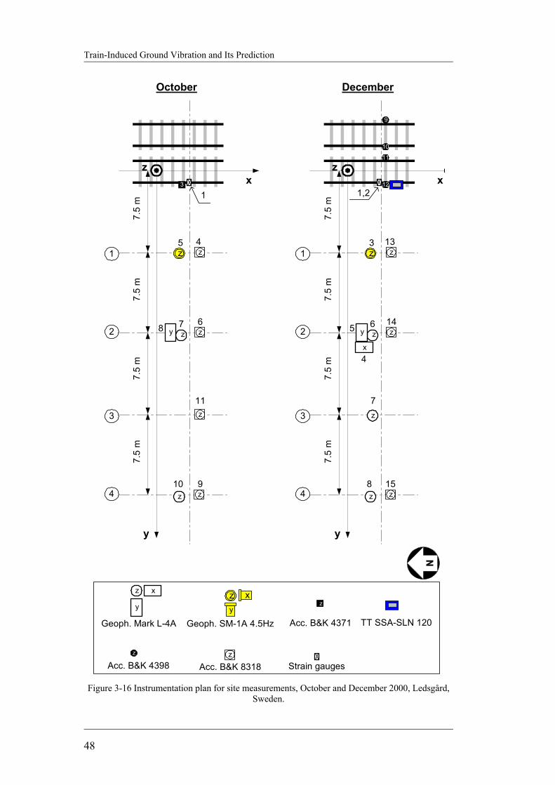
Train-Induced Ground Vibration and Its Prediction
48
zx
y
z
y
x
z
y
xz
x
y z
z
z
z
z
z
z
7.5
m7.
5 m
7.5
m7.
5 m
Geoph. Mark L-4A Geoph. SM-1A 4.5Hz Acc. B&K 4371
Acc. B&K 8318 Strain gauges
1
2
3
4
3
4
6
8
13
14
15
1,2
5
TT SSA-SLN 120
December
7
y
xz
y z
z
z
z
z
z
7.5
m7.
5 m
7.5
m7.
5 m
1
2
3
4
5
7
10
4
6
9
1
8
October
z
Acc. B&K 4398
z
z
11
123
10
11
9
Figure 3-16 Instrumentation plan for site measurements, October and December 2000, Ledsgård,
Sweden.
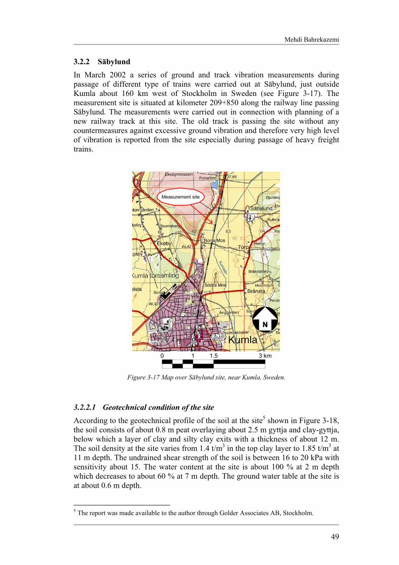
Mehdi Bahrekazemi
49
3.2.2 Säbylund In March 2002 a series of ground and track vibration measurements during passage of different type of trains were carried out at Säbylund, just outside Kumla about 160 km west of Stockholm in Sweden (see Figure 3-17). The measurement site is situated at kilometer 209+850 along the railway line passing Säbylund. The measurements were carried out in connection with planning of a new railway track at this site. The old track is passing the site without any countermeasures against excessive ground vibration and therefore very high level of vibration is reported from the site especially during passage of heavy freight trains.
Measurement site
0 1 1.5 3 km
Figure 3-17 Map over Säbylund site, near Kumla, Sweden.
3.2.2.1 Geotechnical condition of the site
According to the geotechnical profile of the soil at the site5 shown in Figure 3-18, the soil consists of about 0.8 m peat overlaying about 2.5 m gyttja and clay-gyttja, below which a layer of clay and silty clay exits with a thickness of about 12 m. The soil density at the site varies from 1.4 t/m3 in the top clay layer to 1.85 t/m3 at 11 m depth. The undrained shear strength of the soil is between 16 to 20 kPa with sensitivity about 15. The water content at the site is about 100 % at 2 m depth which decreases to about 60 % at 7 m depth. The ground water table at the site is at about 0.6 m depth. 5 The report was made available to the author through Golder Associates AB, Stockholm.

Train-Induced Ground Vibration and Its Prediction
50
The shear wave velocity at the site is estimated to be about 35 m/s in the peat layer, 55 m/s in the gyttja, and about 60 m/s in the clay layer which increases with depth (Bahrekazemi, 2003a).
Figure 3-18. Geotechnical soil properties along at a section at the Säbylund test site.
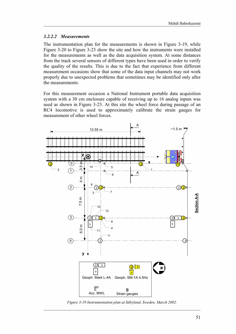
Mehdi Bahrekazemi
51
3.2.2.2 Measurements The instrumentation plan for the measurements is shown in Figure 3-19, while Figure 3-20 to Figure 3-23 show the site and how the instruments were installed for the measurements as well as the data acquisition system. At some distances from the track several sensors of different types have been used in order to verify the quality of the results. This is due to the fact that experience from different measurement occasions show that some of the data input channels may not work properly due to unexpected problems that sometimes may be identified only after the measurements. For this measurement occasion a National Instrument portable data acquisition system with a 30 cm enclosure capable of receiving up to 16 analog inputs was used as shown in Figure 3-23. At this site the wheel force during passage of an RC4 locomotive is used to approximately calibrate the strain gauges for measurement of other wheel forces.
zx
y
z
y
x
y
x
z
z
z
7.5
m4
m
Geoph. Mark L-4A Geoph. SM-1A 4.5Hz
Strain gauges
2
3
4
z
12.55 m ~1.5 m
Sect
ion
A-A
0 zA
A
1214
6.0
m
z
xyz
Acc. MWL
z
1 z3.5
m
z
xz z z
y
5
6
7
8
3
411
1210
z9
13
z
z
z zz
xz z z
y
z
Figure 3-19 Instrumentation plan at Säbylund, Sweden, March 2002.
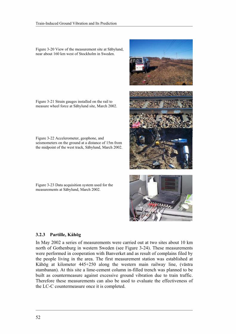
Train-Induced Ground Vibration and Its Prediction
52
Figure 3-20 View of the measurement site at Säbylund, near about 160 km west of Stockholm in Sweden.
Figure 3-21 Strain gauges installed on the rail to measure wheel force at Säbylund site, March 2002.
Figure 3-22 Accelerometer, geophone, and seismometers on the ground at a distance of 15m from the midpoint of the west track, Säbylund, March 2002.
Figure 3-23 Data acquisition system used for the measurements at Säbylund, March 2002.
3.2.3 Partille, Kåhög
In May 2002 a series of measurements were carried out at two sites about 10 km north of Gothenburg in western Sweden (see Figure 3-24). These measurements were performed in cooperation with Banverket and as result of complains filed by the people living in the area. The first measurement station was established at Kåhög at kilometer 445+250 along the western main railway line, (västra stambanan). At this site a lime-cement column in-filled trench was planned to be built as countermeasure against excessive ground vibration due to train traffic. Therefore these measurements can also be used to evaluate the effectiveness of the LC-C countermeasure once it is completed.
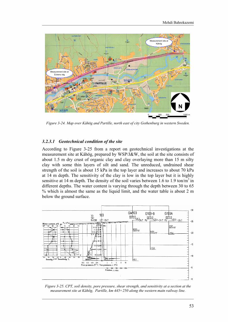
Mehdi Bahrekazemi
53
3.2.3.1 Geotechnical condition of the site According to Figure 3-25 from a report on geotechnical investigations at the measurement site at Kåhög, prepared by WSP/J&W, the soil at the site consists of about 1.5 m dry crust of organic clay and clay overlaying more than 15 m silty clay with some thin layers of silt and sand. The unreduced, undrained shear strength of the soil is about 15 kPa in the top layer and increases to about 70 kPa at 14 m depth. The sensitivity of the clay is low in the top layer but it is highly sensitive at 14 m depth. The density of the soil varies between 1.6 to 1.9 ton/m3 in different depths. The water content is varying through the depth between 30 to 65 % which is almost the same as the liquid limit, and the water table is about 2 m below the ground surface.
Figure 3-25. CPT, soil density, pore pressure, shear strength, and sensitivity at a section at the
measurement site at Kåhög, Partille, km 445+250 along the western main railway line.
0 300 500 1000 m
Measurement site atKåhög
Measurement site atEckens väg
Figure 3-24. Map over Kåhög and Partille, north east of city Gothenburg in western Sweden.
Train-Induced Ground Vibration and Its Prediction
54
The shear wave velocity at this site is estimated to be about 70 m/s in the clay layer and increasing with depth (Bahrekazemi, 2003b).
3.2.3.2 Measurements Ground vibration has been recorded at this site for a variety of train passages including freight trains, passenger trains, commuter trains and high-speed X2000 trains. Passages of trains on both tracks are recorded during measurements, but only the northern track has been equipped with strain gauges to measure the wheel force. Besides measuring ground vibration due to train traffic, Banverket’s measuring car, TLV has been used to measure ground vibration due to simple sinus loadings at different frequencies at this site. During loading the northern track using the hydraulic jack of the TLV, the load has been digitally read directly from the instruments in the measuring car synchronized with the signal from strain gauges attached to the rail. Applying a defined load at a frequency of about 1 Hz, the signal from TLV has been used to calibrate the strain gauges in order to measure the wheel force for passing trains. A number of sensors on the track and the ground have been used to measure particle velocity and/or particle acceleration at different distances from the centerline of the northern track as shown by Figure 3-26. The two SM-1A geophones on the track are place at a distance from each other in order to be able to determine the speed of trains using the signals from them. This will specially be useful if the axle distances of the cars are not known. In those cases the distances between axels are known, the strain gauge signal may also be used to determine the speed of the train (see section 0). Furthermore, using the data from the geophones on the track it would be possible to see how much the difference in the vibration at different locations along the track is. Besides the geophones, two SSA-SLN 120 accelerometers are also mounted on the track. One of them is mounted on the sleeper while the other one is mounted on a steel pedestal that in turn is placed in the ballast as shown by Figure 3-28. These accelerometers may be used to compare the vibration measured in the ballast with that measured on the sleeper. At 15 m and 30 m from the track, all three components of the ground vibration is measured using three sensors, one in each direction as shown in Figure 3-30. One vertical seismometer has been placed at 60 m distance from the centerline of the northern track. At this distance it was predicted that the seismometer would be the only available sensor with enough sensitivity for collecting the vibrations. Figure 3-27 to Figure 3-31 show the site, how different sensors are mounted and the data acquisition system used for the measurements which is a DAT tape recorder together with a laptop computer used for monitoring.
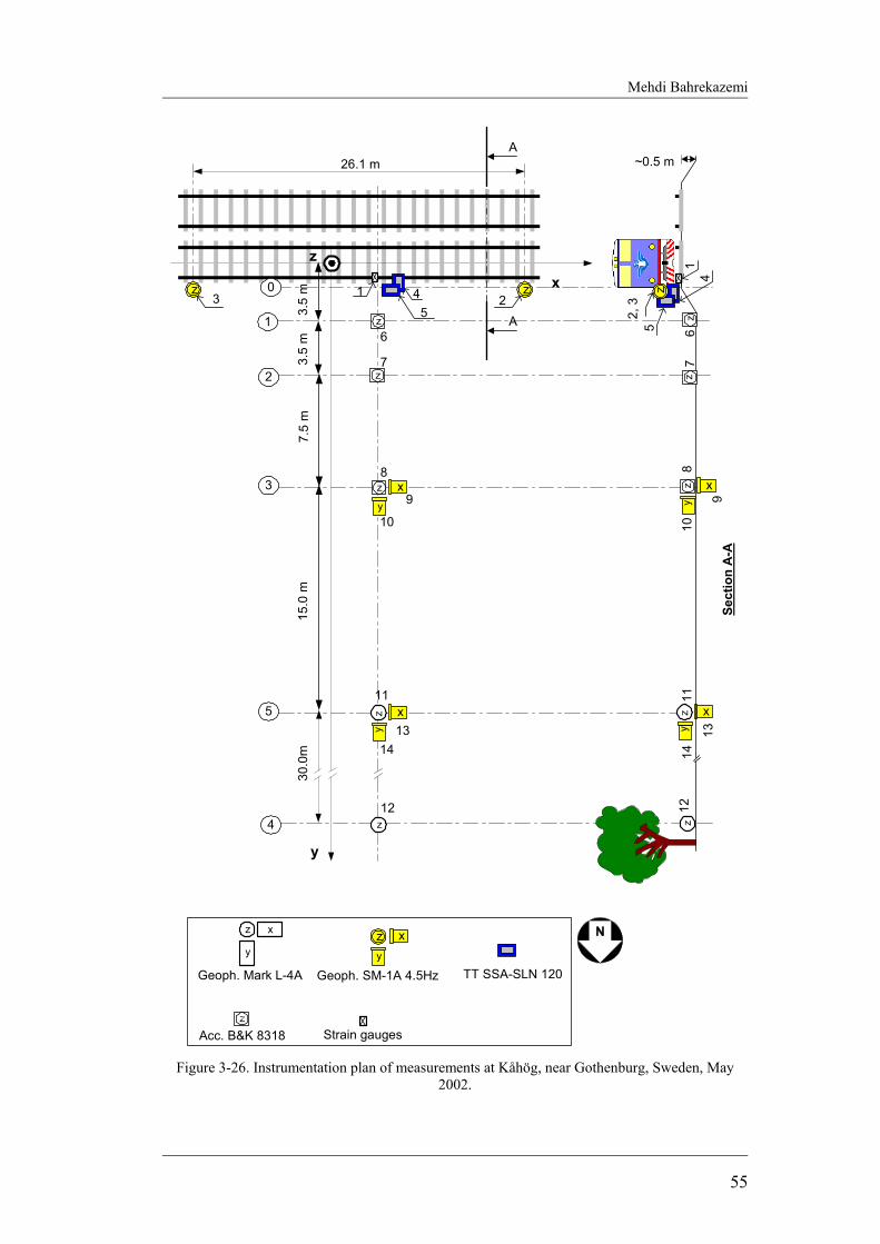
Mehdi Bahrekazemi
55
zx
y
z
y
x
z
y
x
z
z
z
z
z
z
30.0
m15
.0 m
7.5
m3.
5 m
Geoph. Mark L-4A Geoph. SM-1A 4.5Hz
Acc. B&K 8318 Strain gauges
2
3
4
5
12
7
10
TT SSA-SLN 120
z
541z
3 2
26.1 m
13.
5 m
z6
y
x9
8
14y
x13
11
~0.5 m
Sect
ion
A-A
0
z12
z10
y
x
9
8
5
41
z
2, 3
z6
z7
A
A
zy
x13
11
14
Figure 3-26. Instrumentation plan of measurements at Kåhög, near Gothenburg, Sweden, May
2002.
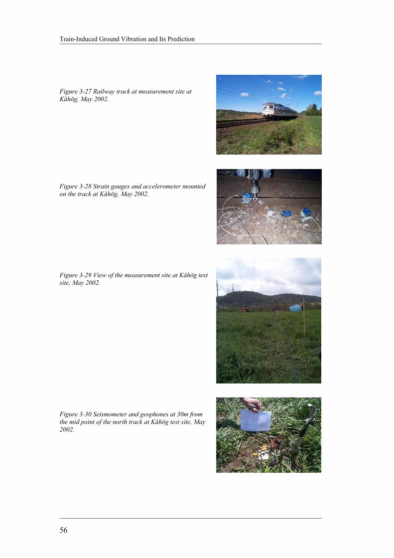
Train-Induced Ground Vibration and Its Prediction
56
Figure 3-27 Railway track at measurement site at Kåhög, May 2002.
Figure 3-28 Strain gauges and accelerometer mounted on the track at Kåhög, May 2002.
Figure 3-29 View of the measurement site at Kåhög test site, May 2002.
Figure 3-30 Seismometer and geophones at 30m from the mid point of the north track at Kåhög test site, May 2002.
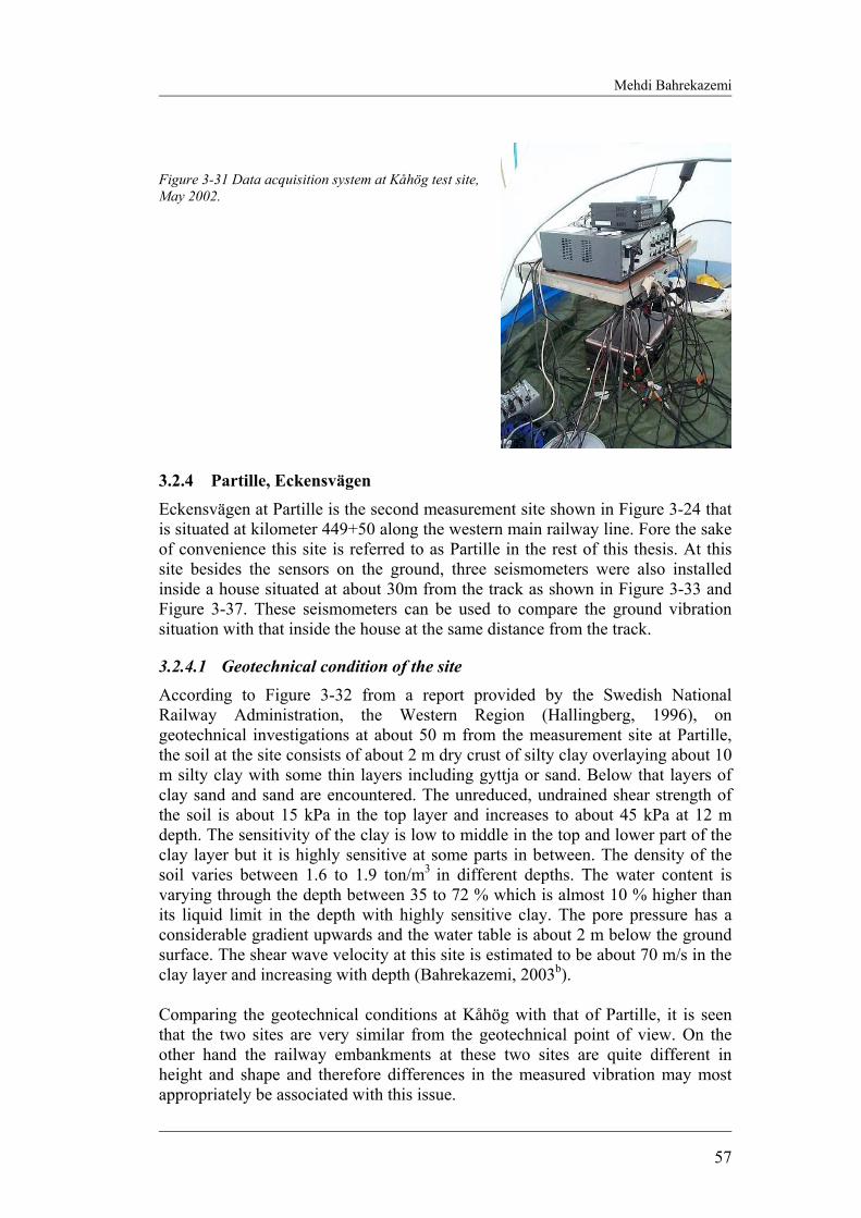
Mehdi Bahrekazemi
57
Figure 3-31 Data acquisition system at Kåhög test site, May 2002.
3.2.4 Partille, Eckensvägen Eckensvägen at Partille is the second measurement site shown in Figure 3-24 that is situated at kilometer 449+50 along the western main railway line. Fore the sake of convenience this site is referred to as Partille in the rest of this thesis. At this site besides the sensors on the ground, three seismometers were also installed inside a house situated at about 30m from the track as shown in Figure 3-33 and Figure 3-37. These seismometers can be used to compare the ground vibration situation with that inside the house at the same distance from the track.
3.2.4.1 Geotechnical condition of the site According to Figure 3-32 from a report provided by the Swedish National Railway Administration, the Western Region (Hallingberg, 1996), on geotechnical investigations at about 50 m from the measurement site at Partille, the soil at the site consists of about 2 m dry crust of silty clay overlaying about 10 m silty clay with some thin layers including gyttja or sand. Below that layers of clay sand and sand are encountered. The unreduced, undrained shear strength of the soil is about 15 kPa in the top layer and increases to about 45 kPa at 12 m depth. The sensitivity of the clay is low to middle in the top and lower part of the clay layer but it is highly sensitive at some parts in between. The density of the soil varies between 1.6 to 1.9 ton/m3 in different depths. The water content is varying through the depth between 35 to 72 % which is almost 10 % higher than its liquid limit in the depth with highly sensitive clay. The pore pressure has a considerable gradient upwards and the water table is about 2 m below the ground surface. The shear wave velocity at this site is estimated to be about 70 m/s in the clay layer and increasing with depth (Bahrekazemi, 2003b). Comparing the geotechnical conditions at Kåhög with that of Partille, it is seen that the two sites are very similar from the geotechnical point of view. On the other hand the railway embankments at these two sites are quite different in height and shape and therefore differences in the measured vibration may most appropriately be associated with this issue.

Train-Induced Ground Vibration and Its Prediction
58
Figure 3-32. CPT, soil density, water table, shear strength, and sensitivity at a section at the measurement site at Eckensvägen, Partille, km 449+009 along the western main railway line.
3.2.4.2 Measurements
The measurement program at this site was very similar to the one at Kåhög. The difference in the instrumentation plan which is shown in Figure 3-33 with the one at Kåhög is in channel 12-14. Here these three seismometers are placed in the middle of the first floor of a house as shown by Figure 3-36 and Figure 3-37 while channel 11 is still on the ground close to the house. Due to the practical issues it was not possible to have enough distance between the seismometer on the ground with the house. This would be more preferable to have some distance in order to be able to measure free field ground vibration at the same distance from the track as the house. Furthermore there was planned to have one accelerometer on the track and one in the ballast at this site too but due too lack of time the accelerometer on the sleeper was not mounted and the one in the ballast did not work. The distance from the sensors to the track is slightly different from that at Kåhög. This is due to practical issues and the fact that it was not possible to have a sensor on the road between the house and the railway. Figure 3-34 to Figure 3-38 show the instrumentation plan and how the sensors where mounted in this site as well as the data acquisition system which is similar to the one at Kåhög. Furthermore the southern track was equipped with strain gauges at this site. Thereby each train would pass on the strain gauges either at Partille or at Kåhög depending on which track they used. This method was chosen as a
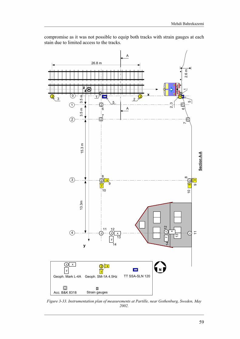
Mehdi Bahrekazemi
59
compromise as it was not possible to equip both tracks with strain gauges at each stain due to limited access to the tracks.
zx
y
z
y
x
z
y
x
z
z
z
z
z
13.3
m15
.3 m
3.5
m
Geoph. Mark L-4A Geoph. SM-1A 4.5Hz
Acc. B&K 8318 Strain gauges
2
3
4
7
10
TT SSA-SLN 120
z
51z
3 2
26.8 m
1
3.5
m
z6
y
x9
8
14
13
11
Sect
ion
A-A
0
x
y
z12
2.6
mz
10y
x9
8
z14
13x
y12
11z
z7
z6
5
z
2, 3
1
A
A
Figure 3-33. Instrumentation plan of measurements at Partille, near Gothenburg, Sweden, May
2002.
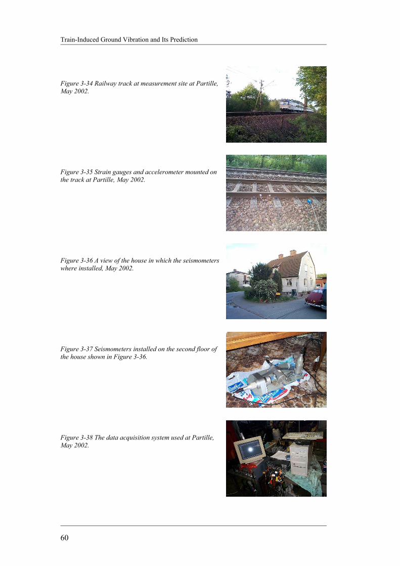
Train-Induced Ground Vibration and Its Prediction
60
Figure 3-34 Railway track at measurement site at Partille, May 2002.
Figure 3-35 Strain gauges and accelerometer mounted on the track at Partille, May 2002.
Figure 3-36 A view of the house in which the seismometers where installed, May 2002.
Figure 3-37 Seismometers installed on the second floor of the house shown in Figure 3-36.
Figure 3-38 The data acquisition system used at Partille, May 2002.
Mehdi Bahrekazemi
61
3.3 MEASUREMENTS PERFORMED BY OTHERS In this section the two measurement occasions performed by other groups than KTH, that have been used for the purpose of this thesis is briefly discussed. The first one is at Ledsgård site, performed by the Swedish National Railway Administration, Banverket and the second one is from a site in Finland, by the name Koria.
3.3.1 Ledsgård
Banverket has performed a series of track and ground vibration measurements at several sites in Sweden during spring 2000 that are reported in two reports, (Johansson 2000a & Johansson 2002b). During the measurements performed at Ledsgård in May 2000, KTH was also present at the site and performed its own vibration measurements on the track and ground. Those measurements performed by KTH are already discussed in section 3.2.1. The data recorded from TT SSA-SLN 120 accelerometers mounted on the sleepers as well as the strain gauges attached to the rail web is among the data made available by Banverket which has been used for the purpose of this work.
3.3.2 Finland, Koria In the frame work of phase1 of NordVib project which is a joint Nordic railway vibration project, it has been decided to conduct an extensive vibration measurement concentrating on detailed study of the impacts of vibration from railway traffic on the built environment along the railway line with aiming at better understanding of wave generation and propagation and for verification of computational tools (Myrvoll et al. 2002). As the Finnish Railway Administration-RHK is currently planning an upgrading of existing line between Lahti and Kouvola for high speed trains (up to 300 km/h) and for more traffic with very heavy trains on soft ground, countermeasures would possibly be necessary to maintain the induced vibrations in the track and environment bellow the allowed limit. One site where vibration countermeasures most possibly must be included is at a site called Koria about 150 km north east of Helsinki in Finland. The location of the test site is shown in Figure 3-39. NGI, the Norwegian Geotechnical Institute has performed the measurements within the framework of Nordvib project and presented in report WP 4B- Field Tests (Myrvoll & Tronstad, 2002) of this project. Nevertheless a brief description of these measurements is presented here for the sake of convenience of the reader.

Train-Induced Ground Vibration and Its Prediction
62
0 300 500 1000 m
Figure 3-39. Map overview of Koria area, Finland (Myrvoll et al. 2002).
3.3.2.1 Geotechnical condition of the site The soil at the test site consists of clay with some layers of possibly sand/silt down to a depth of about 32 m underlying layers of gravel and till material. The water content in the clay layer is between 69-114 % in the layers below the upper layer with liquid limit between 62-72 %. The shear strength is measured by in-situ vane to be 10-23 kPa while it was measured to be 36 kPa by fall-cone test on one sample in the laboratory. The shear wave velocity profile of the soil determined by cross-hole method at two locations is shown in Figure 3-40. According to the figure the shear wave velocity is about 70-90 m/s in the crust layer below which the velocity of the shear wave increases with depth from 60 m/s to about 140 m/s at 14 m depth below the surface. The material damping of the soil vs. shear strain measured from samples taken from different depths is shown Figure 3-41.

Mehdi Bahrekazemi
63
Figure 3-40 Shear wave velocity profile at two sections at Koria test site (Myrvoll et al., 2002).
Figure 3-41. Damping ratio vs. shear strain from laboratory test on samples from Koria test site
(Myrvoll, et al. 2002).
3.3.2.2 Measurements
Figure 3-42 shows the instrumentation plan for the measurements carried out during 8-12 July 2002 at Koria site in Finland (Myrvoll et al. 2002). A number of accelerometers are used to measure particle acceleration at different distances from the track (see Figure 3-46). The northern track is also equipped with strain gauges for measurement of shear and flexural strains. Unfortunately the shear strain gauges are not mounted so that the wheel force may be determined from them directly (see Figure 3-43). Two geophones are also mounted on the foundation of the house as well as on the floor (see Figure 3-44 & Figure 3-45). Figure 3-47 shows parts of the data acquisition system used for the measurements that consists of a DAT tape recorder and a computer.

Train-Induced Ground Vibration and Its Prediction
64
0 3 5 10 m
2.46
2.54
8.00
2.48
2.36
5.14
5.97
10.2
0
1.00
2.45 2.57 2.42 2.60
10.19
13.7
9
Strain gaugesHBM XY41-6/350 & HBM LV41-3/120Acc. PCP 393B12,three axis
Acc. PCP 393B12,two axis
Acc. PCP 393B12,one axis 20.05
Geophone, SM6
4.8
4.71.5
12345
01
23
45
67
89
10
A1_6
A1_2
A1_3
A1_4
A1_5
A1_7
A1_8
A1_9
A1_10
A1_1
A2_6A3_6A4_6A5_6
Floor
foundation
Figure 3-42. Instrumentation plan of measurements at the Koria site (reproduced, Myrvoll et al. 2002).
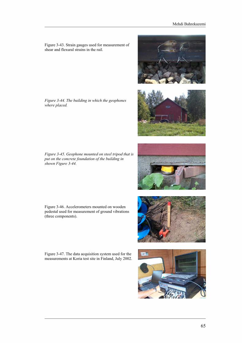
Mehdi Bahrekazemi
65
Figure 3-43. Strain gauges used for measurement of shear and flexural strains in the rail.
Figure 3-44. The building in which the geophones where placed.
Figure 3-45. Geophone mounted on steel tripod that is put on the concrete foundation of the building in shown Figure 3-44.
Figure 3-46. Accelerometers mounted on wooden pedestal used for measurement of ground vibrations (three components).
Figure 3-47. The data acquisition system used for the measurements at Koria test site in Finland, July 2002.

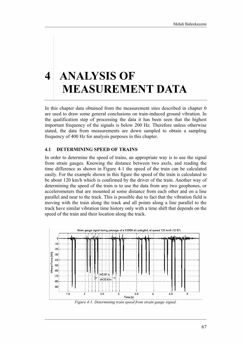
Mehdi Bahrekazemi
67
4 ANALYSIS OF MEASUREMENT DATA
In this chapter data obtained from the measurement sites described in chapter 0 are used to draw some general conclusions on train-induced ground vibration. In the qualification step of processing the data it has been seen that the highest important frequency of the signals is below 200 Hz. Therefore unless otherwise stated, the data from measurements are down sampled to obtain a sampling frequency of 400 Hz for analysis purposes in this chapter.
4.1 DETERMINING SPEED OF TRAINS
In order to determine the speed of trains, an appropriate way is to use the signal from strain gauges. Knowing the distance between two axels, and reading the time difference as shown in Figure 4-1 the speed of the train can be calculated easily. For the example shown in this figure the speed of the train is calculated to be about 120 km/h which is confirmed by the driver of the train. Another way of determining the speed of the train is to use the data from any two geophones, or accelerometers that are mounted at some distance from each other and on a line parallel and near to the track. This is possible due to fact that the vibration field is moving with the train along the track and all points along a line parallel to the track have similar vibration time history only with a time shift that depends on the speed of the train and their location along the track.
Figure 4-1. Determining train speed from strain gauge signal.
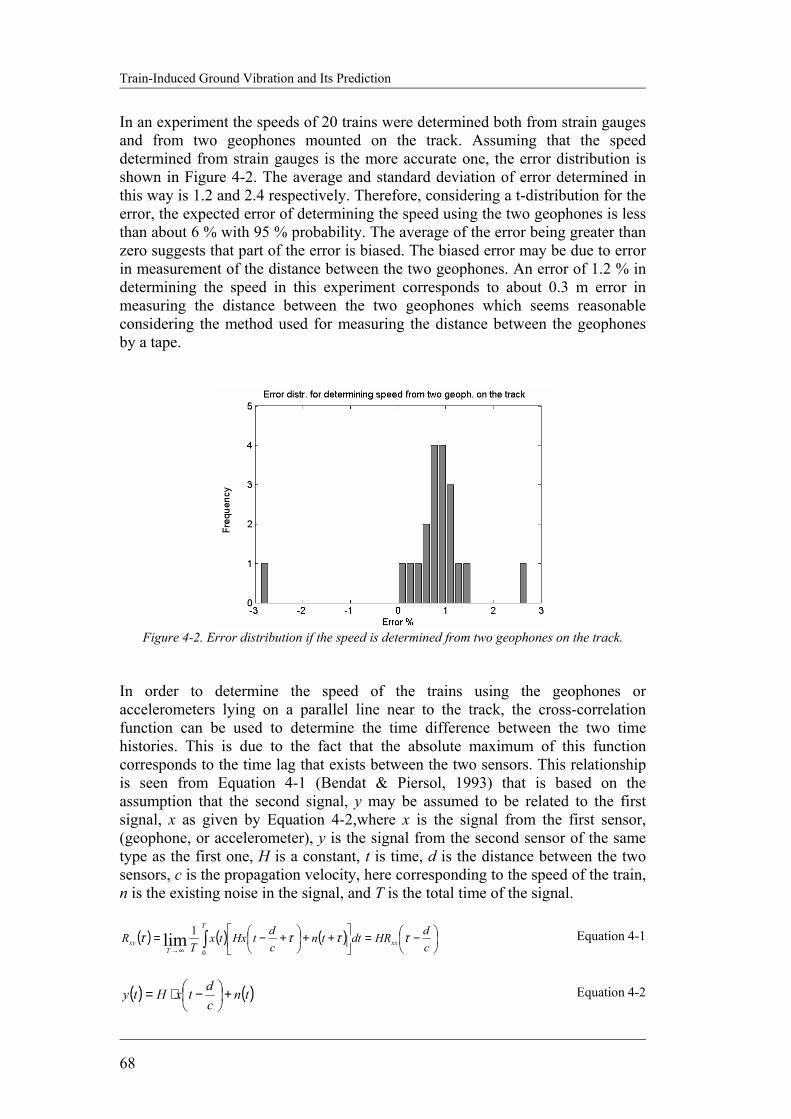
Train-Induced Ground Vibration and Its Prediction
68
In an experiment the speeds of 20 trains were determined both from strain gauges and from two geophones mounted on the track. Assuming that the speed determined from strain gauges is the more accurate one, the error distribution is shown in Figure 4-2. The average and standard deviation of error determined in this way is 1.2 and 2.4 respectively. Therefore, considering a t-distribution for the error, the expected error of determining the speed using the two geophones is less than about 6 % with 95 % probability. The average of the error being greater than zero suggests that part of the error is biased. The biased error may be due to error in measurement of the distance between the two geophones. An error of 1.2 % in determining the speed in this experiment corresponds to about 0.3 m error in measuring the distance between the two geophones which seems reasonable considering the method used for measuring the distance between the geophones by a tape.
Figure 4-2. Error distribution if the speed is determined from two geophones on the track.
In order to determine the speed of the trains using the geophones or accelerometers lying on a parallel line near to the track, the cross-correlation function can be used to determine the time difference between the two time histories. This is due to the fact that the absolute maximum of this function corresponds to the time lag that exists between the two sensors. This relationship is seen from Equation 4-1 (Bendat & Piersol, 1993) that is based on the assumption that the second signal, y may be assumed to be related to the first signal, x as given by Equation 4-2,where x is the signal from the first sensor, (geophone, or accelerometer), y is the signal from the second sensor of the same type as the first one, H is a constant, t is time, d is the distance between the two sensors, c is the propagation velocity, here corresponding to the speed of the train, n is the existing noise in the signal, and T is the total time of the signal.
( ) ( ) ( )
−=
++
+−= ∫
∞→ cdHRdttn
cdtHxtx
TR xx
T
Txy ττττ
0
1lim Equation 4-1
( ) ( )tn
cdtxHty +
−⋅= Equation 4-2
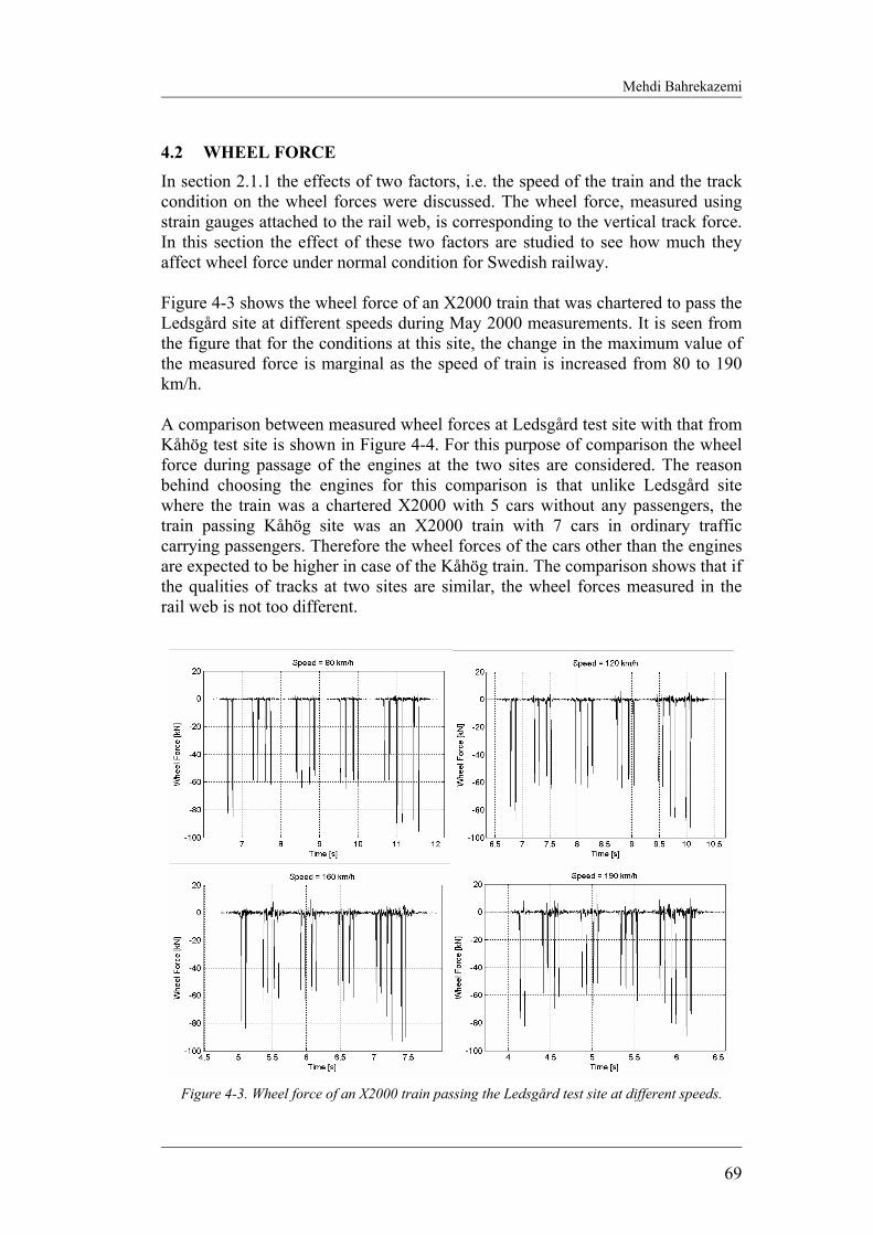
Mehdi Bahrekazemi
69
4.2 WHEEL FORCE In section 2.1.1 the effects of two factors, i.e. the speed of the train and the track condition on the wheel forces were discussed. The wheel force, measured using strain gauges attached to the rail web, is corresponding to the vertical track force. In this section the effect of these two factors are studied to see how much they affect wheel force under normal condition for Swedish railway. Figure 4-3 shows the wheel force of an X2000 train that was chartered to pass the Ledsgård site at different speeds during May 2000 measurements. It is seen from the figure that for the conditions at this site, the change in the maximum value of the measured force is marginal as the speed of train is increased from 80 to 190 km/h. A comparison between measured wheel forces at Ledsgård test site with that from Kåhög test site is shown in Figure 4-4. For this purpose of comparison the wheel force during passage of the engines at the two sites are considered. The reason behind choosing the engines for this comparison is that unlike Ledsgård site where the train was a chartered X2000 with 5 cars without any passengers, the train passing Kåhög site was an X2000 train with 7 cars in ordinary traffic carrying passengers. Therefore the wheel forces of the cars other than the engines are expected to be higher in case of the Kåhög train. The comparison shows that if the qualities of tracks at two sites are similar, the wheel forces measured in the rail web is not too different.
Figure 4-3. Wheel force of an X2000 train passing the Ledsgård test site at different speeds.
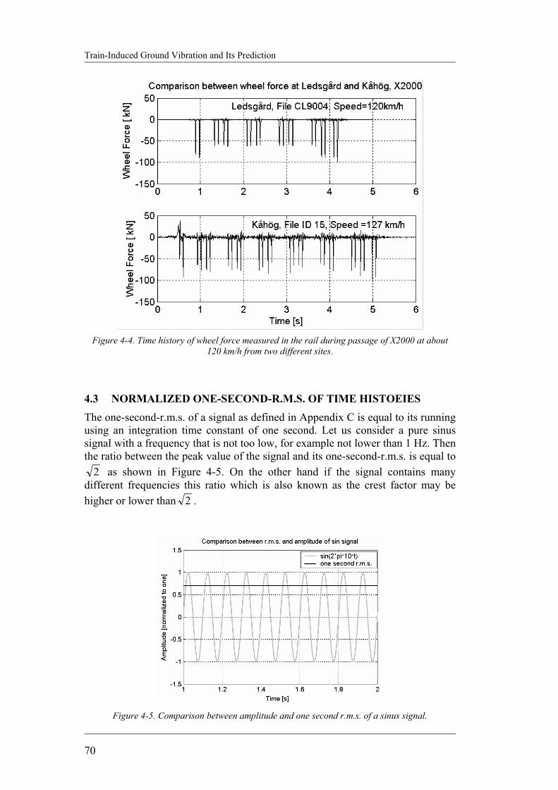
Train-Induced Ground Vibration and Its Prediction
70
Figure 4-4. Time history of wheel force measured in the rail during passage of X2000 at about
120 km/h from two different sites.
4.3 NORMALIZED ONE-SECOND-R.M.S. OF TIME HISTOEIES
The one-second-r.m.s. of a signal as defined in Appendix C is equal to its running using an integration time constant of one second. Let us consider a pure sinus signal with a frequency that is not too low, for example not lower than 1 Hz. Then the ratio between the peak value of the signal and its one-second-r.m.s. is equal to
2 as shown in Figure 4-5. On the other hand if the signal contains many different frequencies this ratio which is also known as the crest factor may be higher or lower than 2 .
Figure 4-5. Comparison between amplitude and one second r.m.s. of a sinus signal.
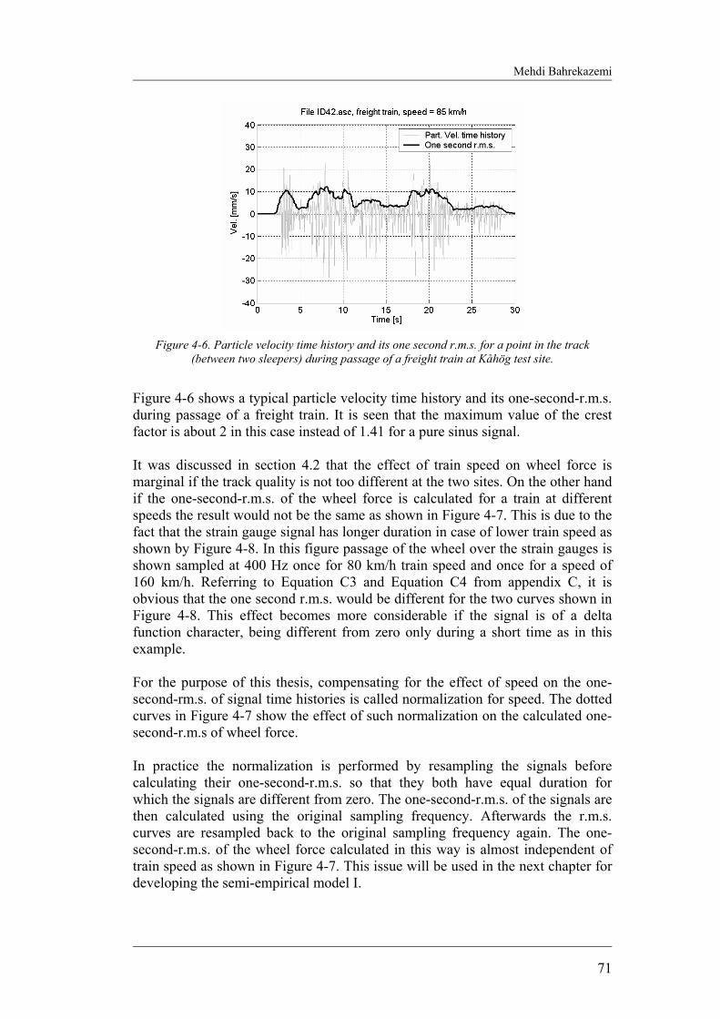
Mehdi Bahrekazemi
71
Figure 4-6. Particle velocity time history and its one second r.m.s. for a point in the track
(between two sleepers) during passage of a freight train at Kåhög test site.
Figure 4-6 shows a typical particle velocity time history and its one-second-r.m.s. during passage of a freight train. It is seen that the maximum value of the crest factor is about 2 in this case instead of 1.41 for a pure sinus signal. It was discussed in section 4.2 that the effect of train speed on wheel force is marginal if the track quality is not too different at the two sites. On the other hand if the one-second-r.m.s. of the wheel force is calculated for a train at different speeds the result would not be the same as shown in Figure 4-7. This is due to the fact that the strain gauge signal has longer duration in case of lower train speed as shown by Figure 4-8. In this figure passage of the wheel over the strain gauges is shown sampled at 400 Hz once for 80 km/h train speed and once for a speed of 160 km/h. Referring to Equation C3 and Equation C4 from appendix C, it is obvious that the one second r.m.s. would be different for the two curves shown in Figure 4-8. This effect becomes more considerable if the signal is of a delta function character, being different from zero only during a short time as in this example. For the purpose of this thesis, compensating for the effect of speed on the one-second-rm.s. of signal time histories is called normalization for speed. The dotted curves in Figure 4-7 show the effect of such normalization on the calculated one-second-r.m.s of wheel force. In practice the normalization is performed by resampling the signals before calculating their one-second-r.m.s. so that they both have equal duration for which the signals are different from zero. The one-second-r.m.s. of the signals are then calculated using the original sampling frequency. Afterwards the r.m.s. curves are resampled back to the original sampling frequency again. The one-second-r.m.s. of the wheel force calculated in this way is almost independent of train speed as shown in Figure 4-7. This issue will be used in the next chapter for developing the semi-empirical model I.

Train-Induced Ground Vibration and Its Prediction
72
Figure 4-7. Effect of normalization for speed on the one-second-r.m.s. of wheel force of an X2000
train at different speeds passing Ledsgård test site in May 2000 (reference speed is 100 km/h).
Figure 4-8. Effect of train speed on sampled wheel force.
4.4 DIFFERENT DIRECTIONAL COMPONENTS OF VIBRATION Figure 4-9 shows the three directional components of vibration on the ground at different distances from the track at Kåhög. It is seen from the figure that the largest component is the vertical one. The parallel horizontal component is on the other hand the smallest one. Similar curves from Partille show that (see Figure 4-10) this conclusion is still valid for the vibrations on the ground. This is despite the change in the relative ratio of the three components. On the other hand the curves corresponding to the sensors inside the building show that the transverse horizontal component is much higher (almost twice) than the vertical component at low frequencies (the amplitude of vibration is the highest for these frequencies). This should be kept in mind while estimating vibrations inside buildings. In the rest of this thesis only the vertical component of the vibration is considered unless otherwise stated.
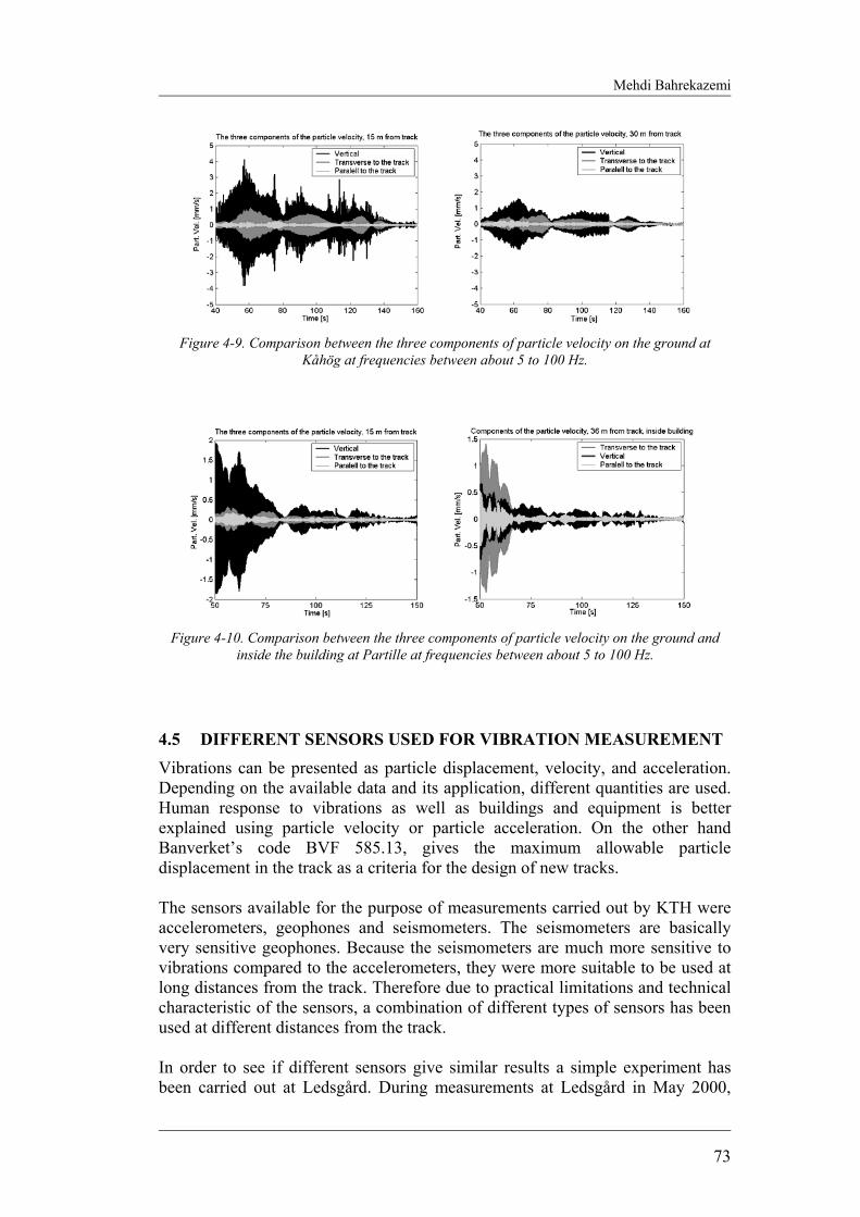
Mehdi Bahrekazemi
73
4.5 DIFFERENT SENSORS USED FOR VIBRATION MEASUREMENT Vibrations can be presented as particle displacement, velocity, and acceleration. Depending on the available data and its application, different quantities are used. Human response to vibrations as well as buildings and equipment is better explained using particle velocity or particle acceleration. On the other hand Banverket’s code BVF 585.13, gives the maximum allowable particle displacement in the track as a criteria for the design of new tracks. The sensors available for the purpose of measurements carried out by KTH were accelerometers, geophones and seismometers. The seismometers are basically very sensitive geophones. Because the seismometers are much more sensitive to vibrations compared to the accelerometers, they were more suitable to be used at long distances from the track. Therefore due to practical limitations and technical characteristic of the sensors, a combination of different types of sensors has been used at different distances from the track. In order to see if different sensors give similar results a simple experiment has been carried out at Ledsgård. During measurements at Ledsgård in May 2000,
Figure 4-9. Comparison between the three components of particle velocity on the ground at
Kåhög at frequencies between about 5 to 100 Hz.
Figure 4-10. Comparison between the three components of particle velocity on the ground and
inside the building at Partille at frequencies between about 5 to 100 Hz.
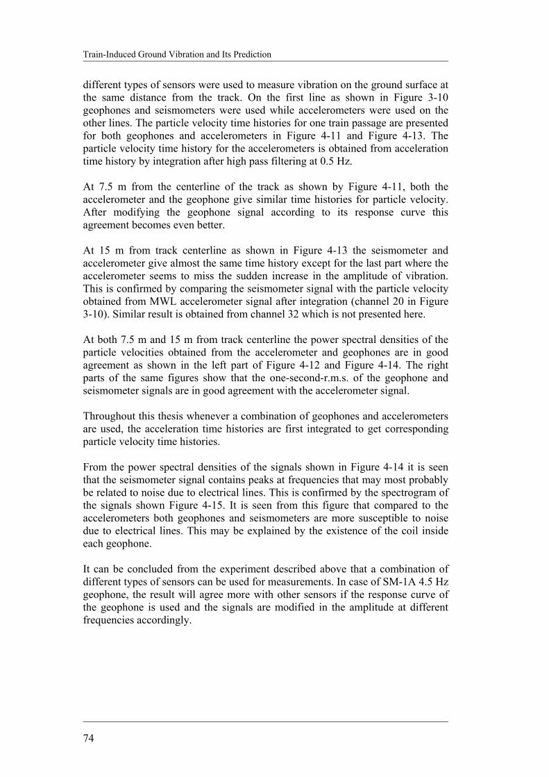
Train-Induced Ground Vibration and Its Prediction
74
different types of sensors were used to measure vibration on the ground surface at the same distance from the track. On the first line as shown in Figure 3-10 geophones and seismometers were used while accelerometers were used on the other lines. The particle velocity time histories for one train passage are presented for both geophones and accelerometers in Figure 4-11 and Figure 4-13. The particle velocity time history for the accelerometers is obtained from acceleration time history by integration after high pass filtering at 0.5 Hz. At 7.5 m from the centerline of the track as shown by Figure 4-11, both the accelerometer and the geophone give similar time histories for particle velocity. After modifying the geophone signal according to its response curve this agreement becomes even better. At 15 m from track centerline as shown in Figure 4-13 the seismometer and accelerometer give almost the same time history except for the last part where the accelerometer seems to miss the sudden increase in the amplitude of vibration. This is confirmed by comparing the seismometer signal with the particle velocity obtained from MWL accelerometer signal after integration (channel 20 in Figure 3-10). Similar result is obtained from channel 32 which is not presented here. At both 7.5 m and 15 m from track centerline the power spectral densities of the particle velocities obtained from the accelerometer and geophones are in good agreement as shown in the left part of Figure 4-12 and Figure 4-14. The right parts of the same figures show that the one-second-r.m.s. of the geophone and seismometer signals are in good agreement with the accelerometer signal. Throughout this thesis whenever a combination of geophones and accelerometers are used, the acceleration time histories are first integrated to get corresponding particle velocity time histories. From the power spectral densities of the signals shown in Figure 4-14 it is seen that the seismometer signal contains peaks at frequencies that may most probably be related to noise due to electrical lines. This is confirmed by the spectrogram of the signals shown Figure 4-15. It is seen from this figure that compared to the accelerometers both geophones and seismometers are more susceptible to noise due to electrical lines. This may be explained by the existence of the coil inside each geophone. It can be concluded from the experiment described above that a combination of different types of sensors can be used for measurements. In case of SM-1A 4.5 Hz geophone, the result will agree more with other sensors if the response curve of the geophone is used and the signals are modified in the amplitude at different frequencies accordingly.
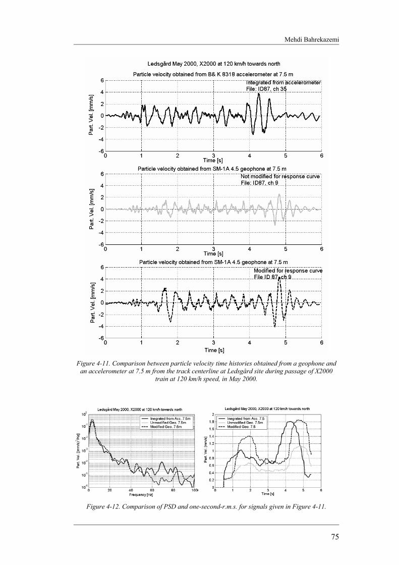
Mehdi Bahrekazemi
75
Figure 4-11. Comparison between particle velocity time histories obtained from a geophone and
an accelerometer at 7.5 m from the track centerline at Ledsgård site during passage of X2000 train at 120 km/h speed, in May 2000.
Figure 4-12. Comparison of PSD and one-second-r.m.s. for signals given in Figure 4-11.

Train-Induced Ground Vibration and Its Prediction
76
Figure 4-13. Comparison between particle velocity time histories obtained from a seismometer
and an accelerometer at 15 m from the track centerline at Ledsgård site during passage of X2000 train at 120 km/h speed, in May 2000.
Figure 4-14. Comparison of PSD and one-second-r.m.s. for signals given in Figure 4-13.
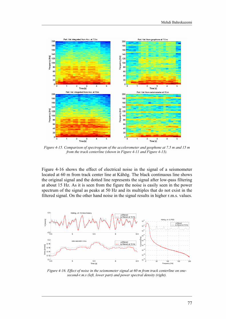
Mehdi Bahrekazemi
77
Figure 4-15. Comparison of spectrogram of the accelerometer and geophone at 7.5 m and 15 m
from the track centerline (shown in Figure 4-11 and Figure 4-13).
Figure 4-16 shows the effect of electrical noise in the signal of a seismometer located at 60 m from track center line at Kåhög. The black continuous line shows the original signal and the dotted line represents the signal after low-pass filtering at about 15 Hz. As it is seen from the figure the noise is easily seen in the power spectrum of the signal as peaks at 50 Hz and its multiples that do not exist in the filtered signal. On the other hand noise in the signal results in higher r.m.s. values.
4.5 5 5.5 6 6.5-0.5
0
0.5
V [m
m/s
]
Kåhög, ch 12 time history
4.5 5 5.5 6 6.50.1
0.12
0.14
0.16
0.18
0.2
Time [s]
Vrm
s [m
m/s
]
one-second-r.m.s.
unfilteredlp filtered at 15 Hz
unfilteredlp filtered at 15 Hz
0 50 100 150 20010
-18
10-16
10-14
10-12
10-10
10-8
10-6
10-4
10-2 Kåhög, ch 12 PSD
Frequency [Hz]
V [(
mm
/s)2 /H
z]
unfilteredlp filtered at 15 Hz
Figure 4-16. Effect of noise in the seismometer signal at 60 m from track centerline on one-
second-r.m.s (left, lower part) and power spectral density (right).

Train-Induced Ground Vibration and Its Prediction
78
4.6 LOCATION OF THE SENSOR As the quality of the track varies at different parts, some variation is expected in the generation of the vibrations in the source. The energy of vibration propagates from the source to the surrounding through mediums. Both material and geometrical damping result in attenuation of vibration with distance from the source. The frequency content of the vibration may also change from source to the receiver. These issues are studied in this section using measurement data from several sites.
4.6.1 Comparing vibration in the ballast with sleeper At Kåhög site another accelerometer of the same kind as the one mounted on the sleeper was installed in the ballast between two sleepers (see Figure 3-28). These two accelerometers can be used to compare the vibration in the ballast with vibration on the sleeper (which is usually measured by Banverket). It is seen from Figure 4-17 that the acceleration time history corresponding to the sleeper has higher amplitude. This conclusion is further confirmed if the power spectral densities of the two signals are studied as shown in Figure 4-18. Similarly the time histories for particle velocity and particle displacement shown in Figure 4-19 and Figure 4-20 respectively reveal that this difference is inherited from acceleration. One of the quantities that are widely used throughout this thesis is the one second r.m.s. value of the particle velocity. A comparison between the r.m.s. values of the particle velocity for a point on the sleeper and in the ballast is shown in Figure 4-21. The figure clearly shows higher vibration of the sleeper compared to the ballast.
Figure 4-17. Acceleration time histories on a sleeper and in the ballast during passage of X2000
train at about 120 km/h at Kåhög..

Mehdi Bahrekazemi
79
Figure 4-18. Power spectral densities of the acceleration time histories shown in Figure 4-17.
Figure 4-19. Velocity time histories on a sleeper and ballast during passage of X2000 train at
about 120 km/h at Kåhög.

Train-Induced Ground Vibration and Its Prediction
80
Figure 4-20.Displacement time histories on a sleeper and ballast during passage of X2000 train
at about 120 km/h. at Kåhög.
Figure 4-21. Comparison between r.m.s. of the particle velocity for a point on the sleeper and a
point in the ballast at Kåhög site during passage of a X2000 train at about 120 km/h.
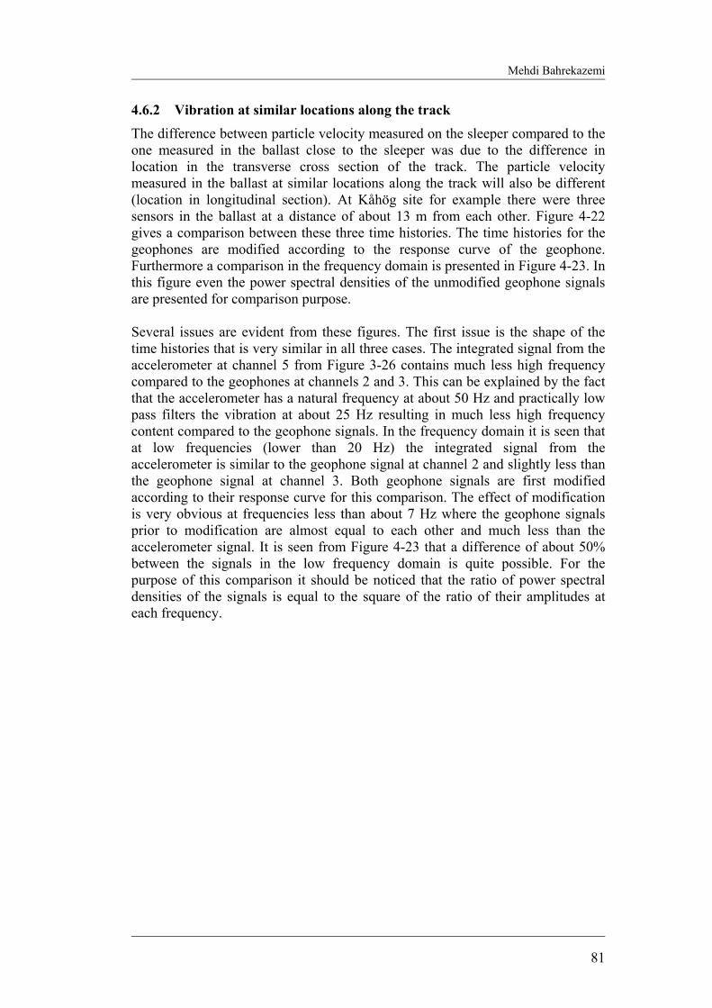
Mehdi Bahrekazemi
81
4.6.2 Vibration at similar locations along the track The difference between particle velocity measured on the sleeper compared to the one measured in the ballast close to the sleeper was due to the difference in location in the transverse cross section of the track. The particle velocity measured in the ballast at similar locations along the track will also be different (location in longitudinal section). At Kåhög site for example there were three sensors in the ballast at a distance of about 13 m from each other. Figure 4-22 gives a comparison between these three time histories. The time histories for the geophones are modified according to the response curve of the geophone. Furthermore a comparison in the frequency domain is presented in Figure 4-23. In this figure even the power spectral densities of the unmodified geophone signals are presented for comparison purpose. Several issues are evident from these figures. The first issue is the shape of the time histories that is very similar in all three cases. The integrated signal from the accelerometer at channel 5 from Figure 3-26 contains much less high frequency compared to the geophones at channels 2 and 3. This can be explained by the fact that the accelerometer has a natural frequency at about 50 Hz and practically low pass filters the vibration at about 25 Hz resulting in much less high frequency content compared to the geophone signals. In the frequency domain it is seen that at low frequencies (lower than 20 Hz) the integrated signal from the accelerometer is similar to the geophone signal at channel 2 and slightly less than the geophone signal at channel 3. Both geophone signals are first modified according to their response curve for this comparison. The effect of modification is very obvious at frequencies less than about 7 Hz where the geophone signals prior to modification are almost equal to each other and much less than the accelerometer signal. It is seen from Figure 4-23 that a difference of about 50% between the signals in the low frequency domain is quite possible. For the purpose of this comparison it should be noticed that the ratio of power spectral densities of the signals is equal to the square of the ratio of their amplitudes at each frequency.

Train-Induced Ground Vibration and Its Prediction
82
Figure 4-22. Comparison of particle velocity measured at different location in the track at Kåhög
site.
Figure 4-23. Comparison of particle velocity PSD measured at different location along the track
at Kåhög site in two different scales.
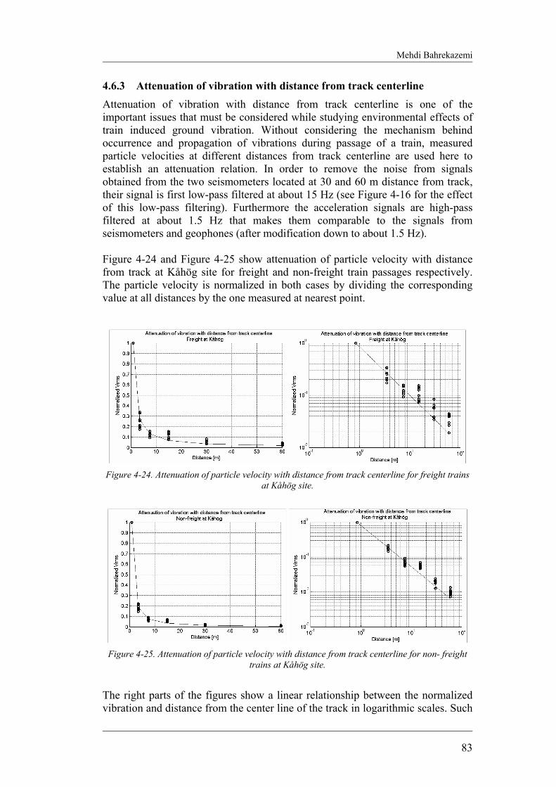
Mehdi Bahrekazemi
83
4.6.3 Attenuation of vibration with distance from track centerline Attenuation of vibration with distance from track centerline is one of the important issues that must be considered while studying environmental effects of train induced ground vibration. Without considering the mechanism behind occurrence and propagation of vibrations during passage of a train, measured particle velocities at different distances from track centerline are used here to establish an attenuation relation. In order to remove the noise from signals obtained from the two seismometers located at 30 and 60 m distance from track, their signal is first low-pass filtered at about 15 Hz (see Figure 4-16 for the effect of this low-pass filtering). Furthermore the acceleration signals are high-pass filtered at about 1.5 Hz that makes them comparable to the signals from seismometers and geophones (after modification down to about 1.5 Hz). Figure 4-24 and Figure 4-25 show attenuation of particle velocity with distance from track at Kåhög site for freight and non-freight train passages respectively. The particle velocity is normalized in both cases by dividing the corresponding value at all distances by the one measured at nearest point.
Figure 4-24. Attenuation of particle velocity with distance from track centerline for freight trains
at Kåhög site.
Figure 4-25. Attenuation of particle velocity with distance from track centerline for non- freight
trains at Kåhög site.
The right parts of the figures show a linear relationship between the normalized vibration and distance from the center line of the track in logarithmic scales. Such
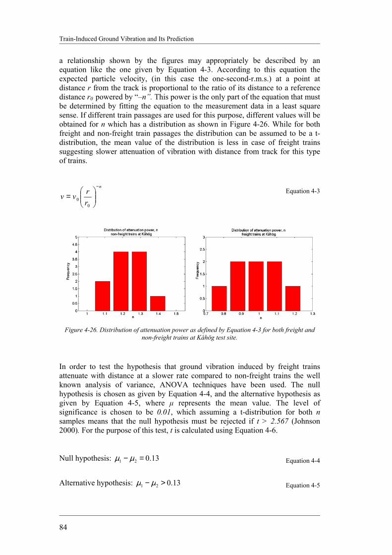
Train-Induced Ground Vibration and Its Prediction
84
a relationship shown by the figures may appropriately be described by an equation like the one given by Equation 4-3. According to this equation the expected particle velocity, (in this case the one-second-r.m.s.) at a point at distance r from the track is proportional to the ratio of its distance to a reference distance r0 powered by “–n”. This power is the only part of the equation that must be determined by fitting the equation to the measurement data in a least square sense. If different train passages are used for this purpose, different values will be obtained for n which has a distribution as shown in Figure 4-26. While for both freight and non-freight train passages the distribution can be assumed to be a t-distribution, the mean value of the distribution is less in case of freight trains suggesting slower attenuation of vibration with distance from track for this type of trains.
n
rrvv
−
=
00
Equation 4-3
Figure 4-26. Distribution of attenuation power as defined by Equation 4-3 for both freight and
non-freight trains at Kåhög test site.
In order to test the hypothesis that ground vibration induced by freight trains attenuate with distance at a slower rate compared to non-freight trains the well known analysis of variance, ANOVA techniques have been used. The null hypothesis is chosen as given by Equation 4-4, and the alternative hypothesis as given by Equation 4-5, where µ represents the mean value. The level of significance is chosen to be 0.01, which assuming a t-distribution for both n samples means that the null hypothesis must be rejected if t > 2.567 (Johnson 2000). For the purpose of this test, t is calculated using Equation 4-6. Null hypothesis: 13.021 =− µµ Equation 4-4
Alternative hypothesis: 13.021 >− µµ Equation 4-5

Mehdi Bahrekazemi
85
704.211
)(
21
21 =+
−−=
nnS
XXt
p
δ Equation 4-6
where, ( ) ( )
211
21
222
2112
−+−+−
=nn
SnSnS p , 0.06781 =S , 1.18681 =X , 111 =n ,
1235.02 =S , 9377.02 =X , 82 =n , and δ=0.13 Because the calculated t-value according to Equation 4-6 is greater than 2.567, the null hypothesis must be rejected which means that with 99% probability the mean value of attenuation power n in case of freight trains is 0.13 less than that of non-freight trains. For the test result to be valid the variances of the two samples should not be too different. As a rule of thumb, if one variance is four times the other, the result of the test is not reliable (Johnson, 2000). As it is presented above, the ratio of the two variances is about 1.8 which confirms the validity of the test. The lower power of attenuation in case of freight trains may be explained by the fact that freight trains are usually much longer than non-freight trains and therefore are more like a linear source compared to non-freight trains. Using measurement data from Partille, Figure 4-27 and Figure 4-28 have been prepared that show how particle velocity attenuates with distance from the track at this site. It is seen from these figures that the general shapes of the curves are similar to those from the Kåhög site. The mean value of n in case of freight trains is 1.0076 and the standard deviation is 0.1210. Corresponding values in case of non-freight trains are 1.1967 and 0.0440 respectively. An analysis of variances similar to the one described above reveals that the difference between the samples means for attenuation power n, determined for Kåhög and Partille is not significant.
Figure 4-27. Attenuation of particle velocity with distance from track centerline for freight trains
at the Partille test site (four passages are used for this figure).

Train-Induced Ground Vibration and Its Prediction
86
Figure 4-28. Attenuation of particle velocity with distance from track centerline for non- freight
trains at the Partille test site (three passages are used for this figure).
At the Ledsgård site as it is seen from Figure 4-29 attenuation of vibration with distance from the centerline of track is different for different train speeds. While in case of low speed passages (80 and 120 km/h with attenuation power of about 1.19) the attenuation curve is very similar to that of Kåhög and Partille, at higher speeds some abnormalities are seen. It is seen from the figure that as the speed is increased, particle velocity attenuates more slowly with distance from track. Especially for the point located at 7.5 m from track centerline, vibration is as much as or even higher than that measured in the track. Examining the quality of the signals it was observed that for 170 and 190 km/h train speed, the sensors at 7.5 m and 15 m from the centerline of the track used for this analysis had missed the highest peaks of the vibration due to saturation of the channel (vibration had been beyond the dynamic range chosen for the channel at the site). This explains why in some cases the data points corresponding to 170 and 190 km/h speeds are lower than the data points corresponding to speeds 160 and 170 km/h in the figure. At Ledsgård the critical speed of the track has been estimated to be about 235 km/h (Madshus & Kaynia, 2000). The results shown in Figure 4-29 show that at about 60% of the critical speed of the track, the attenuation curve obtained for low speed trains will seriously underestimate ground vibration close to the track. Measurements from the test site at Säbylund show also a similar situation for train speeds as low as about 130 km/h according to Figure 4-30. There is only one freight train passage available from the measurements at Säbylund that has good signal quality at all channels. The attenuation power for this passage excluding the closest point to the track as outlier is calculated to be 0.94 which is within the range obtained for freight trains at Kåhög and Partille (see Figure 4-31). For non-freight trains the slowest passage available is one with 119 km/h speed as shown in Figure 4-32 the attenuation power for this passage excluding the nearest point to the track is 1.28 which also is within the range of those obtained from the other sites. On the other hand like Ledsgård, here too the attenuation with distance diverts from the low speed curve as the speed of trains increase. The hypothesis that ground vibration on a line perpendicular to the track attenuates slower as train speed approaches the Rayleigh wave speed of the

Mehdi Bahrekazemi
87
mediumhas been theoretically studied using a simplified analytical model (Bodare, 1999). As a conclusion while using attenuation relations it must be investigated first that the speed of the train is slow compared to the critical speed in order to avoid underestimation of vibration in the vicinity of the track.
Figure 4-29. Attenuation of vibration at Ledsgård site for different train speeds. There are several passages available for each speed but only one is presented in the figure for the sake of simplicity.
The data points from other passages are very close to those shown in the figure.
Figure 4-30. Attenuation of vibration at Säbylund site for different train speeds.
Figure 4-31. Attenuation with distance from track centerline for freight train at Säbylund site.

Train-Induced Ground Vibration and Its Prediction
88
Figure 4-32. Attenuation with distance from track centerline for non- freight trains at Säbylund.
4.7 EFFECT OF WHEEL/TRAIN LOAD ON GROUND-BORNE VIBRATION
Figure 4-33 shows the effect of wheel force as discussed in section 4.2 on measured particle velocity for freight trains at Kåhög test site. Using one-second-r.m.s. of wheel force and particle velocity time histories during passage of one freight train, the effect of wheel force is isolated from the effect of train speed. It is seen from the figure that there is a clear correlation between wheel force and particle velocity with a correlation factor of 0.93 measured for this case. The best line fitted to the data, in the least square sense, does not go through the origin as expected. On the other hand there have not been so many data points in the vicinity of origin and therefore the line should be modified for this and is forced to go through the origin for the purpose of this study. The fitted line presents a linear relationship between wheel force and particle velocity at a constant train speed.

Mehdi Bahrekazemi
89
4.8 EFFECT OF TRAIN SPEED ON GROUND-BORNE VIBRATION In order to study the effect of train speed, the one-second-r.m.s. of particle velocity and wheel force time histories are first determined for trains of the same type passing each test site at different speeds. The maximum value of the one second-r.m.s. of the particle velocity time history is then divided by the maximum value of the one-second-r.m.s. calculated for the wheel force time history. In this way the effects of site conditions, wheel force and train type are isolated from the effect of train speed. Figure 4-34 to Figure 4-36 show the relationship between particle velocity and train speed for trains at three different sites. The origin has been assumed to be a data point in all three cases as experience shows that a train at rest causes no ground vibration. As it is seen from Figure 4-34 to Figure 4-36 three different speed zones may be identified defining the relation between train speed and induced vibration. The first zone is indicated as zone one in the figures and extends from zero to approximately 30 km/h train speed (the upper limit of the zone may be different depending on soil type). In this zone the particle velocity in the track increases with train speed. The dashed line approximates the relationship between train speed and particle velocity in this zone. Due to lack of data point in this zone it is not possible to exactly determine the slope of the line. The second zone that begins at about 30 km/h and extends to about 80 km/h is the region where the particle velocity in the track is more or less constant irrespective
Figure 4-33. Effect of wheel force (measured in the rail) on particle velocity in the track.
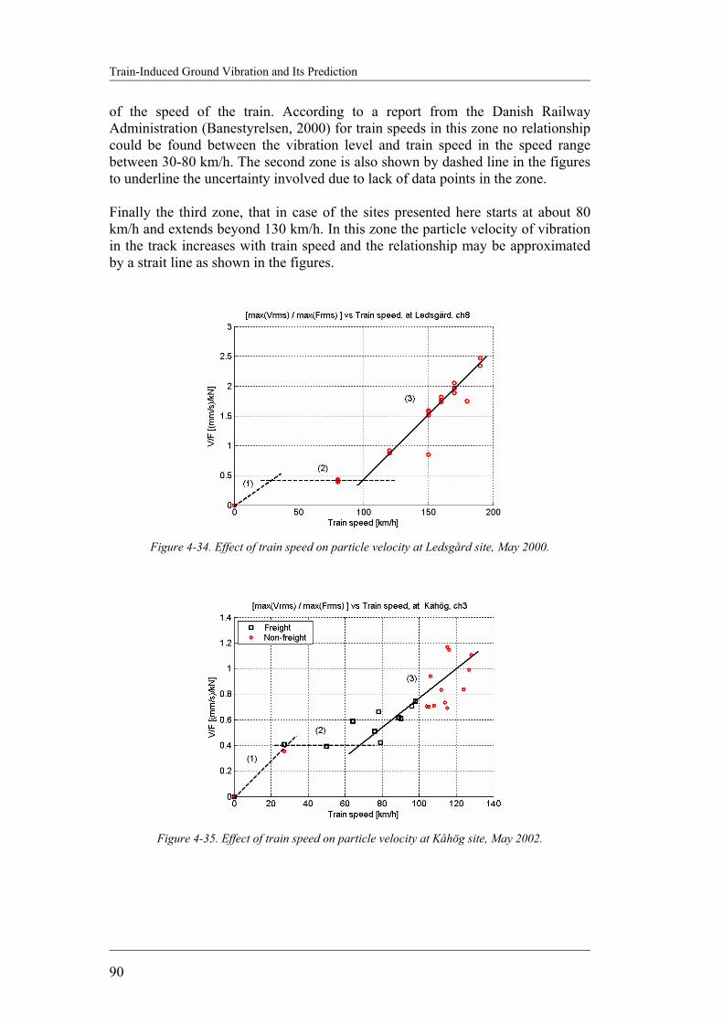
Train-Induced Ground Vibration and Its Prediction
90
of the speed of the train. According to a report from the Danish Railway Administration (Banestyrelsen, 2000) for train speeds in this zone no relationship could be found between the vibration level and train speed in the speed range between 30-80 km/h. The second zone is also shown by dashed line in the figures to underline the uncertainty involved due to lack of data points in the zone. Finally the third zone, that in case of the sites presented here starts at about 80 km/h and extends beyond 130 km/h. In this zone the particle velocity of vibration in the track increases with train speed and the relationship may be approximated by a strait line as shown in the figures.
Figure 4-34. Effect of train speed on particle velocity at Ledsgård site, May 2000.
Figure 4-35. Effect of train speed on particle velocity at Kåhög site, May 2002.
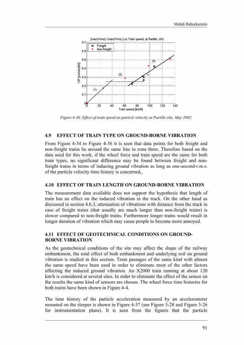
Mehdi Bahrekazemi
91
Figure 4-36. Effect of train speed on particle velocity at Partille site, May 2002.
4.9 EFFECT OF TRAIN TYPE ON GROUND-BORNE VIBRATION
From Figure 4-34 to Figure 4-36 it is seen that data points for both freight and non-freight trains lie around the same line in zone three. Therefore based on the data used for this work, if the wheel force and train speed are the same for both train types, no significant difference may be found between freight and non-freight trains in terms of inducing ground vibration as long as one-second-r.m.s. of the particle velocity time history is concerned,.
4.10 EFFECT OF TRAIN LENGTH ON GROUND-BORNE VIBRATION
The measurement data available does not support the hypothesis that length of train has an effect on the induced vibration in the track. On the other hand as discussed in section 4.6.3, attenuation of vibrations with distance from the track in case of freight trains (that usually are much longer than non-freight trains) is slower compared to non-freight trains. Furthermore longer trains would result in longer duration of vibration which may cause people to become more annoyed.
4.11 EFFECT OF GEOTECHNICAL CONDITIONS ON GROUND-BORNE VIBRATION
As the geotechnical conditions of the site may affect the shape of the railway embankment, the total effect of both embankment and underlying soil on ground vibration is studied in this section. Train passages of the same kind with almost the same speed have been used in order to eliminate most of the other factors affecting the induced ground vibration. An X2000 train running at about 120 km/h is considered at several sites. In order to eliminate the effect of the sensor on the results the same kind of sensors are chosen. The wheel force time histories for both trains have been shown in Figure 4-4. The time history of the particle acceleration measured by an accelerometer mounted on the sleeper is shown in Figure 4-37 (see Figure 3-28 and Figure 3-26 for instrumentation plans). It is seen from the figures that the particle
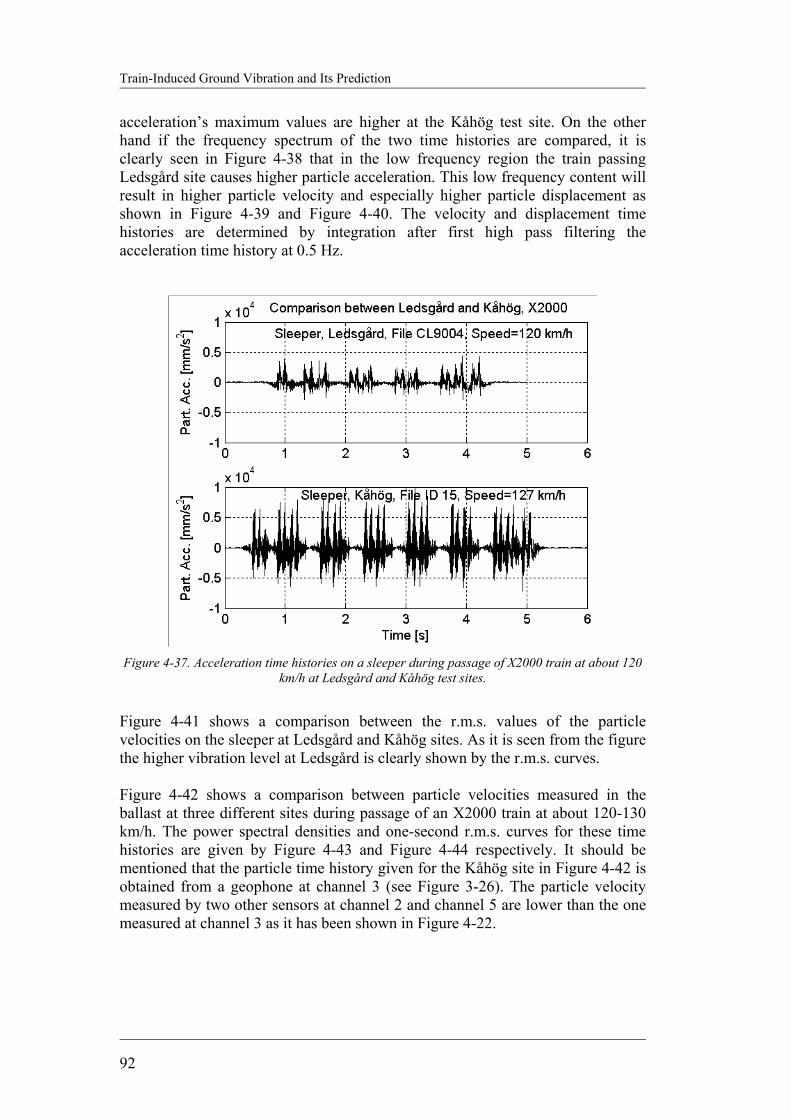
Train-Induced Ground Vibration and Its Prediction
92
acceleration’s maximum values are higher at the Kåhög test site. On the other hand if the frequency spectrum of the two time histories are compared, it is clearly seen in Figure 4-38 that in the low frequency region the train passing Ledsgård site causes higher particle acceleration. This low frequency content will result in higher particle velocity and especially higher particle displacement as shown in Figure 4-39 and Figure 4-40. The velocity and displacement time histories are determined by integration after first high pass filtering the acceleration time history at 0.5 Hz.
Figure 4-37. Acceleration time histories on a sleeper during passage of X2000 train at about 120
km/h at Ledsgård and Kåhög test sites.
Figure 4-41 shows a comparison between the r.m.s. values of the particle velocities on the sleeper at Ledsgård and Kåhög sites. As it is seen from the figure the higher vibration level at Ledsgård is clearly shown by the r.m.s. curves. Figure 4-42 shows a comparison between particle velocities measured in the ballast at three different sites during passage of an X2000 train at about 120-130 km/h. The power spectral densities and one-second r.m.s. curves for these time histories are given by Figure 4-43 and Figure 4-44 respectively. It should be mentioned that the particle time history given for the Kåhög site in Figure 4-42 is obtained from a geophone at channel 3 (see Figure 3-26). The particle velocity measured by two other sensors at channel 2 and channel 5 are lower than the one measured at channel 3 as it has been shown in Figure 4-22.
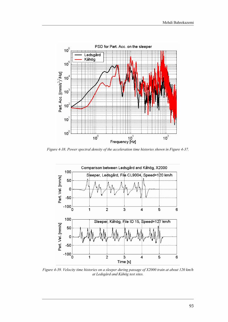
Mehdi Bahrekazemi
93
Figure 4-38. Power spectral density of the acceleration time histories shown in Figure 4-37.
Figure 4-39. Velocity time histories on a sleeper during passage of X2000 train at about 120 km/h
at Ledsgård and Kåhög test sites.
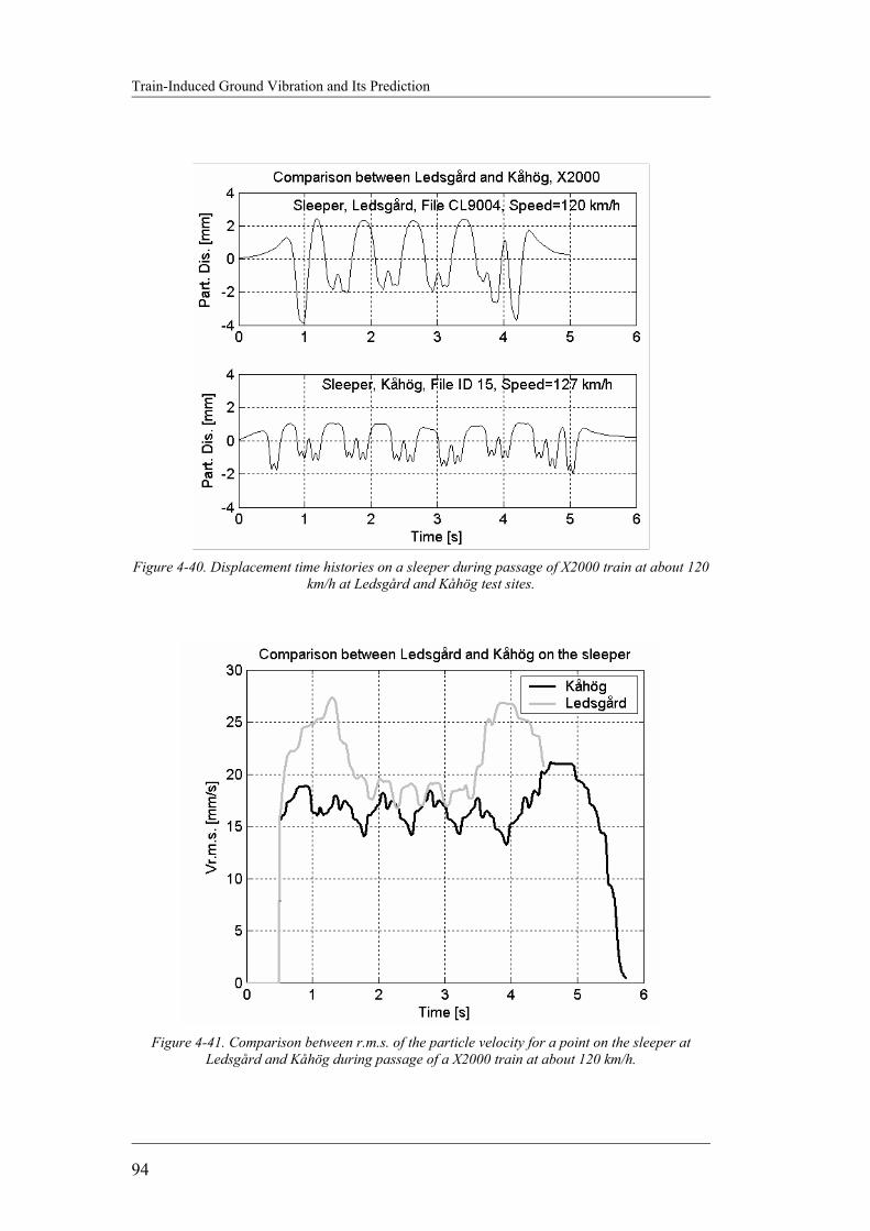
Train-Induced Ground Vibration and Its Prediction
94
Figure 4-40. Displacement time histories on a sleeper during passage of X2000 train at about 120
km/h at Ledsgård and Kåhög test sites.
Figure 4-41. Comparison between r.m.s. of the particle velocity for a point on the sleeper at
Ledsgård and Kåhög during passage of a X2000 train at about 120 km/h.

Mehdi Bahrekazemi
95
Figure 4-42. Comparison between particle velocity in the ballast at three sites, Ledsgård, Kåhög,
and Partille for similar train passage.
Figure 4-43. Comparison between PSD of particle velocity in the ballast at three sites, Ledsgård, Kåhög, and Partille for similar train passage in two different scales
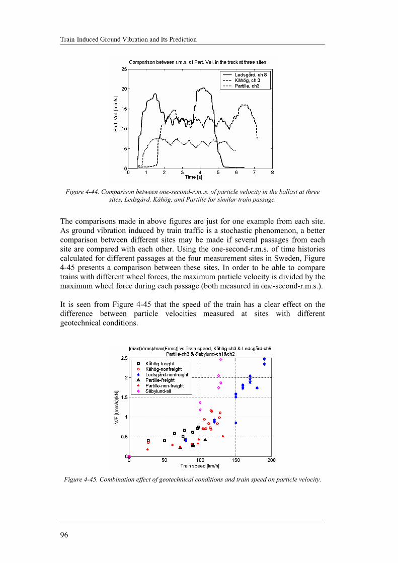
Train-Induced Ground Vibration and Its Prediction
96
Figure 4-44. Comparison between one-second-r.m..s. of particle velocity in the ballast at three
sites, Ledsgård, Kåhög, and Partille for similar train passage.
The comparisons made in above figures are just for one example from each site. As ground vibration induced by train traffic is a stochastic phenomenon, a better comparison between different sites may be made if several passages from each site are compared with each other. Using the one-second-r.m.s. of time histories calculated for different passages at the four measurement sites in Sweden, Figure 4-45 presents a comparison between these sites. In order to be able to compare trains with different wheel forces, the maximum particle velocity is divided by the maximum wheel force during each passage (both measured in one-second-r.m.s.). It is seen from Figure 4-45 that the speed of the train has a clear effect on the difference between particle velocities measured at sites with different geotechnical conditions.
Figure 4-45. Combination effect of geotechnical conditions and train speed on particle velocity.

Mehdi Bahrekazemi
97
4.12 VIBRATION IN BUILDINGS Generally the vertical component of vibration decreases propagating through different stories of buildings (DOT-T-95-16, 1995). The horizontal components on the other hand may increase as discussed in section 4.4 of this report. Unfortunately there are not enough measurement data available to the author to conduct a statistical study on the effect of buildings on ground-borne vibration due to train traffic.
4.13 EFFECT OF SOME COUNTERMEASURES Measurements performed at the Ledsgård site before and after stabilization of the soil under west track by lime-cement columns have been used to evaluate the effectiveness of soil stabilization method as a countermeasure against excessive ground vibration induced by train traffic (Bahrekazemi et al. 2003). The measurements show that the peak to peak amplitude of particle displacement is reduced by a factor about 5 for trains running at low speeds, while it has reduced about 15 times for high-speed trains. This is expected as the dynamic amplification due to the critical speed effects has been removed from the vibrations using the soil stabilization method. Furthermore the measurements show that despite the fact that only soil improvement has been carried out under the west track, ground vibration are mitigated even when trains pass on the untreated east track (about 20%). This is thought to be partly due to the fact that the lime-cement column walls under the west track work somewhat as a barrier (in-filled trench) in the way of vibrations from the east track (Bahrekazemi et al., 2001).
4.14 SUMMARY OF CONCLUSIONS FROM THE MEASUREMENTS A comparison of wheel forces from an X2000 train passing the Ledsgård test site at different speeds shows that the change in the amplitude of the measured force is marginal as the speed of train is increased from 80 to 190 km/h. This suggests that for modern boogies and with normal track conditions, the speed of train does not affect the dynamic wheel forces measured in the rail dramatically. Furthermore a comparison between wheel forces of two X2000 trains from two different test sites shows that if the conditions of the tracks at the sites are not too different, the wheel forces measured at these two sites will not be too different either. The data shows that usually the vertical component of vibration is the largest one, but inside the buildings one of the horizontal components may become the largest component depending on the natural frequencies of the building in different directions, and the location of the sensor inside the building. Although it is preferable to use the same type of sensor in all locations at the measurements, similar results will be obtained from different sensor types mounted in similar situations if a combination of them is used.
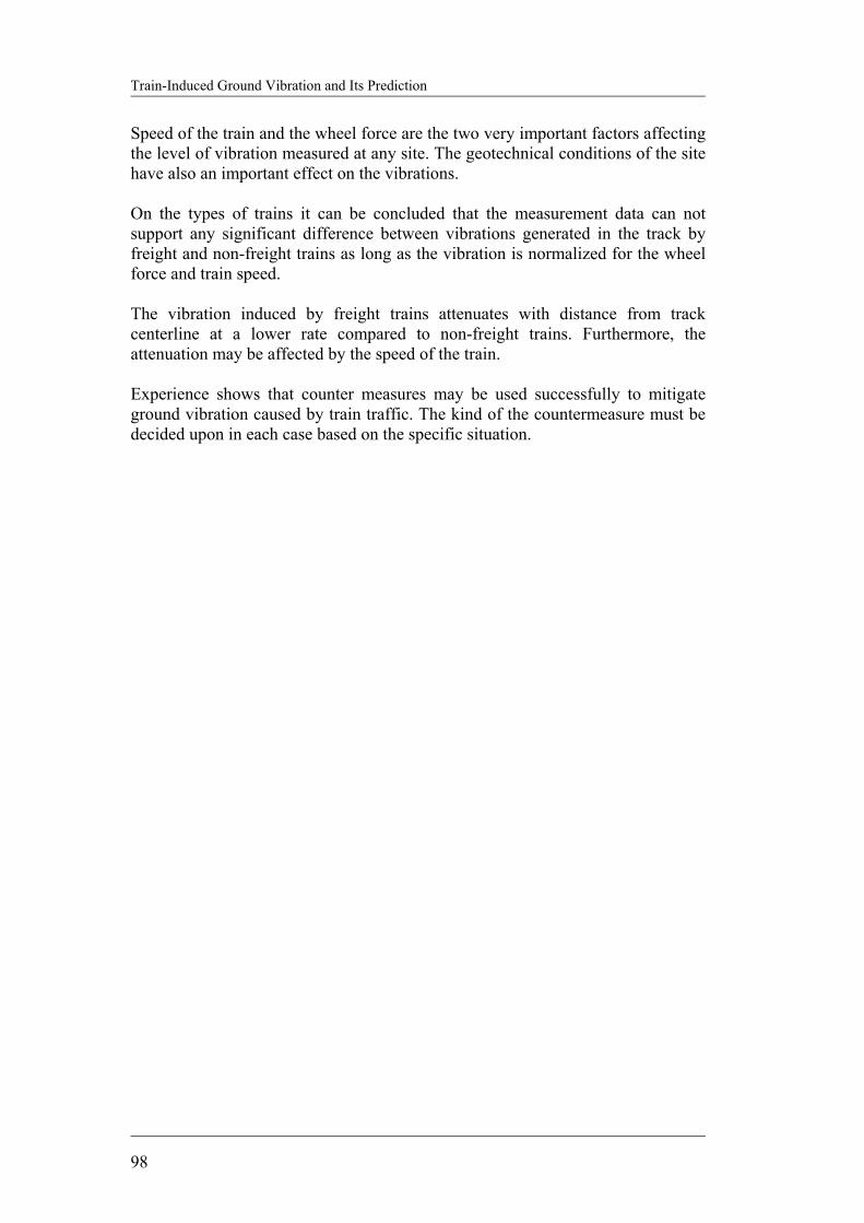
Train-Induced Ground Vibration and Its Prediction
98
Speed of the train and the wheel force are the two very important factors affecting the level of vibration measured at any site. The geotechnical conditions of the site have also an important effect on the vibrations. On the types of trains it can be concluded that the measurement data can not support any significant difference between vibrations generated in the track by freight and non-freight trains as long as the vibration is normalized for the wheel force and train speed. The vibration induced by freight trains attenuates with distance from track centerline at a lower rate compared to non-freight trains. Furthermore, the attenuation may be affected by the speed of the train. Experience shows that counter measures may be used successfully to mitigate ground vibration caused by train traffic. The kind of the countermeasure must be decided upon in each case based on the specific situation.
Mehdi Bahrekazemi
99
5 ENVIB SEMI-EMPIRICAL MODEL, CLASS I
In this chapter a semi-empirical model based on measurement data from the test sites in Sweden described in chapter 0 is presented. The model relates the one-second-r.m.s.6 of the particle velocity on the track7 with the one-second-r.m.s. of the wheel force and speed of the train at each site. The effect of the geotechnical conditions and embankment shapes at the sites are also briefly discussed in order to give general guide lines in using the model. In order to determine the limits within which the expected error of the model may lie, a statistical analysis of the estimation error is also performed and presented. Furthermore the model is verifyd using measurement data that have not been used in the development process of the model. Finally the integration of the model with a GIS system that can be used both for calculation and presentation of the model results is discussed.
5.1 THE STRUCTURE OF THE MODEL AND ITS PARAMETERS The first site considered is the Kåhög test site. The measurement data from this site is used to determine the parameters of the model as described in this section. It was discussed in chapter 1 that the one-second-r.m.s. of particle velocity in the track varies with the one-second-r.m.s. of the wheel force and speed of the train as well as several other parameters. Therefore, all parameters affecting the particle velocity are kept constant at a time except for one. This way the effect of each parameter is isolated from the others. Furthermore, the trains are primarily categorized in two different categories, i.e. freight trains and non-freight trains. Freight trains include all kind of trains with different lengths and different kind of cars that are used for transport of goods. The non-freight category on the other hand includes all types of passenger, regional, and commuter trains, as well as the X2000 high speed train. Although it was discussed in section 4.9 that the type of train does not have a significant effect on the particle velocity measured on the track, the parameters of the model are once determined for each train category separately and once for all trains put together. The results are then compared with each other at the end of this section.
6 Throughout this chapter the one-second-r.m.s. is normalized for train speed. 7 For a point 0.85 m from the track centerline

Train-Induced Ground Vibration and Its Prediction
100
An important factor affecting the vibration as stated by many authors (for example Madshus & Kaynia, 1999, Krylov, 2001, and Bahrekazemi & Hildebrand, 2001) and as discussed in section 4.8 is the speed of the train. Figure 5-1 shows the distribution of speeds for train passages recorded at the Kåhög site for different train types. Unfortunately enough data is not available for train passages with speeds covering the whole range from very low to very high speeds for this site. This is due to the fact that the measurements are performed under ordinary traffic conditions for the site that for example means that X2000 high-speed trains pass the site at much lower speed than their maximum speed, which is 200 km/h. This implies that using the model outside this speed range may result in higher error than expected.
Figure 5-1. Speed range of different train types recorded at Kåhög site.
Another important factor to consider for the model is the wheel force as discussed in section 4.7. In order to study the effect of this factor, all train passages with speeds corresponding to zone 3 as shown in Figure 4-35 are chosen. The one-second-r.m.s. of wheel forces, Frms and particle velocity in the track, Vrms are then determined as shown for one example in Figure 4-33 (right lower part). For this purpose parts of the signals that include too much noise or abnormalities are removed during data qualification step. For the example presented in Figure 4-33 the selected part is shown by black color. A linear relationship is then established between Vrms and Frms similar to the one shown in the left lower part of the same figure. In the next step the Vrms corresponding to a number of wheel forces, Frms are determined for all train passages. In this case Frms is chosen between 10-30 kN. For each wheel force a linear relationship is then established between the particle velocity, Vrms and train speeds. The result is a series of lines as shown in Figure 5-2 (left upper part). The general equation for these lines is given by Equation 5-1, for which the two parameters, a and b are determined as a function of wheel force, Frms as shown by Figure 5-3.

Mehdi Bahrekazemi
101
Figure 5-2. Relation between particle velocity in the track and train’s speed and wheel force at the
Kåhög site.
Figure 5-3. Relationship between the parameters of Equation 5-1 with wheel force, Frms
corresponding to the lower part of Figure 5-2.
bspeedaVrms +⋅= Equation 5-1
where 21 aFaa rms +⋅= , and 21 bFbb rms +⋅=
,,, 121 baa and 2b are presented in Table 5-1 for all the sites discussed in this section, and speed is the speed of the train in km/h, while Vrms is in mm/s.

Train-Induced Ground Vibration and Its Prediction
102
In order to determine the confidence interval corresponding to a certain probability, the difference between the estimated Vrms obtained from Equation 5-1 and the corresponding measured Vrms is calculated for all train passages. The regression error of the model is then defined by Equation 5-2.
calculatedVrmsmeasuredVrmscalculatedVrmsError
,,, −= Equation 5-2
The error defined by Equation 5-2 has a distribution as shown in Figure 5-4. Using this distribution the error corresponding to any certain probability can be determined. For the distribution shown in Figure 5-4 the 10% and 90% probabilities are marked with two squares. The wheel force, Frms at the Kåhög site has a distribution as shown in Figure 5-5. The values corresponding to 95% and 99% probabilities are shown in the figure with a square and a star respectively. Similar figures as this figure prepared (not presented here) for the other three sites in Sweden has shown that Frms corresponding to the 95% and 99% probabilities are almost the same at all sites. The continuous line shown in Figure 5-6 gives the relationship between particle velocity on the track and train speed at Kåhög site assuming Frms to be 25 kN, which is close to the wheel force corresponding to 99% probability. The dashed lines in the figure are corresponding to 10% and 90% probabilities respectively. According to Figure 5-6 only in 10% of cases the particle velocity estimated by Equation 5-1 for the Kåhög site has an error more than about 30%.
Figure 5-4. Distribution of error, as defined by Equation 5-2.
Mehdi Bahrekazemi
103
Figure 5-5. Distribution of one second r.m.s. of the wheel force, Frms at Kåhög. The square on the
figure corresponds to 95% probability and the star to 99% probability.
Figure 5-6. Dependence of particle velocity on the track on train speed at Kåhög. Dashed lines
correspond to 10 % and 90 % probabilities respectively.
In the same way as described for the Kåhög site, the parameters of Equation 5-1 are determined for the other three test sites at Partille, Ledsgård, and Säbylund.These parameters together with some additional information about these sites are presented in Table 5-1. The relations between Vrms and train speed at these sites for Frms equal to 25 kN are shown in Figure 5-7 to Figure 5-9. It is seen from Figure 5-6, Figure 5-7, and Figure 5-8 that the distances between the dashed lines and the continuous line at Ledsgård and Partille test sites are similar to that of Kåhög. On the other hand Figure 5-9 shows relatively low regression error at Säbylund test site (the dashed lines are close to the continuous line). The reason for this low error is that at this site only a few passages with speeds very close to each other have been used for determining the parameters of Equation 5-1.
Train-Induced Ground Vibration and Its Prediction
104
Figure 5-7. Dependence of particle velocity in the track on train speed at Partille. Dashed lines
correspond to 10 % and 90 % probabilities respectively.
Figure 5-8. Dependence of particle velocity in the track on train speed at Ledsgård. Dashed lines
correspond to 10 % and 90% probabilities respectively.
Figure 5-9. Dependence of particle velocity in the track on train speed at Säbylund. Dashed lines
correspond to 10 % and 90 % probabilities respectively.
Mehdi Bahrekazemi
105
Figure 5-10 shows a comparison between the models obtained based on freight, non-freight, and all train types at the Kåhög test site. It is seen from this figure that the three lines corresponding to these three different set of data are very close to each other especially in case of the model for Partille (lower part of the figure), and the one based on data from the TT accelerometer at Kåhög (right upper part of the same figure). On the other hand it is seen that the model based on the accelerometer data (corresponding to ch5) gives slightly lower estimation compared to the model based on the geophone (corresponding to ch3) at Kåhög. This may be explained by the fact that the accelerometer signal is practically low-pass filtered at about 25 Hz due to characteristic curve of the sensor as discussed in chapter 0.
Figure 5-10. Comparison between models based on data from freight, non freight, and all kinds of
trains. For data channel’s identification see Figure 3-26 and Figure 3-33. Figure 5-11compares the models corresponding to the Kåhög site with that of Partille. Although the geotechnical conditions of these two sites are very similar as discussed in chapter 0, the railway embankment at Partille has a higher height compared to that at Kåhög. At Partille about 50 m after the test site towards Gothenburg a railway bridge is built over a road and therefore the embankment at this site has a higher height than that at Kåhög. Figure 5-12 compares the models corresponding to the sites at Kåhög and Ledsgård. As it is seen from the figure the line corresponding to Ledsgård has steeper slope. This may be related to the differences in the geotechnical conditions at theses two sites.

Train-Induced Ground Vibration and Its Prediction
106
Figure 5-11. Effect of railway embankment’s height on the particle velocity estimated by the
models based on Equation 5-1 for a point on the track.
Figure 5-12. Effect of the underlying soil on the particle velocity estimated by the models based on
Equation 5-1 for a point on the track.
Table 5-1. Summary of the model parameters obtained for the four different sites in Sweden.
a [(mm/s)/(km/h)]
b [(mm/s)/(km/h)]
Model error n*
Site Emb. height
[m] cs
[m/s] a1 a2 b1 b2 µ [mm/s]
б [mm/s]
µ б
0.937 0.124 Kåhög ~1 ~70 0.007 0.000 0.022 0.001 -0.034 0.201
1.187 .068 1.001 0.121
Partille ~2.5 ~70 0.006 0.000 -0.212 0.001 -0.091 0.238 1.197 .044 NA NA
Ledsgård ~1.4 ~45 0.024 0.000 -1.548 0.001 -0.060 0.271 1.188** 0.015 0.941 NA***
Säbylund ~1.5 ~35 0.028 0.000 -1.423 0.001 -0.059 0.099 1.285 NA***
cs: Shear wave velocity of the soil in the upper layers, (just under the crust). a & b: The parameters of the model defined for Equation 5-1 µ: Mean value б: Standard deviation n: Attenuation power according to Equation 4-3 * The smaller attenuation power n, corresponds to freight trains. ** This attenuation power is obtained from train passages at 80 km/h. *** Only one sample is available for this case, which is given in the table instead of µ.
Mehdi Bahrekazemi
107
The semi-empirical model for estimation of particle velocity, Vrms at a point on the ground can now be presented by putting together Equation 4-3 and Equation 5-1 as in Equation 5-3.
( )n
rms rrbspeedaV
−
+⋅=
0
Equation 5-3
where, 21 aFaa rms +⋅= , 21 bFbb rms +⋅= , r0 is the reference distance here taken as 0.85 m, r is the distance from the point for which the prediction is made to the track centerline, n is the attenuation power according to Table 5-1, speed is the speed of the train in km/h, and Vrms is the estimated one-second-r.m.s. of the particle velocity in mm/s. If accurate information about the traffic on the railway is not available, the one-second-r.m.s. of the wheel force, Frms which is needed as an input to Equation 5-3 can be determined using Figure 5-5. According to the histogram presented in Figure 5-5, Frms = 25 kN corresponds to a wheel force that will not be exceeded with 99% probability.
5.2 VERIFICATION OF THE MODEL
In order to verify the model some parts of the data was put aside and not used in determining the parameters of the model. Figure 5-13 shows the time histories of the wheel force and particle velocities at two different points together with their one-second-r.m.s. during passage of an X2000 train at the Kåhög site. The speed of the train in this case is about 127 km/h. Figure 5-14 shows a comparison between measured and calculated one-second-r.m.s. of the particle velocities on the track at Kåhög. As it is seen from the figure the predicted values are very close to the measured ones. The dashed line presents the border above which only 10 % of the measured Vrms values are expected to lie. The dotted line on the other hand shows the limit below which 10 % of the corresponding measured values may lie. Figure 5-15 shows a comparison between measured and calculated one-second-r.m.s. of the particle velocities at a point 30 m from the centerline of the track. It is seen from the figure that the measured values are between the dashed and the dotted lines. The continuous black line in this figure is obtained from the continuous black line shown in Figure 5-14 after modifying for the attenuation according to Equation 4-3. The attenuation power used for this line is the mean value for the Kåhög site presented in Table 5-1. The dashed line on the other hand has been obtained based on the dashed line in Figure 5-14. The attenuation power used in this case corresponds to the limit below which only 10 % of the attenuation powers are expected to lie. In a similar way the dotted line in Figure 5-15 is based on the dotted line in Figure 5-14 after modification for attenuation using the attenuation power corresponding to 90 % probability.

Train-Induced Ground Vibration and Its Prediction
108
Figure 5-13. Time history and its one-second-r.m.s. of the wheel force and particle velocity during
passage of an X2000 train at Kåhög.
Figure 5-14. Comparison between measured and calculated r.m.s. of particle velocity time history
on the track using the Class I model for an X2000 train at Kåhög.
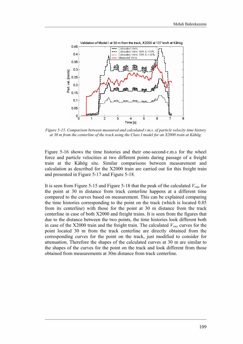
Mehdi Bahrekazemi
109
Figure 5-15. Comparison between measured and calculated r.m.s. of particle velocity time history
at 30 m from the centerline of the track using the Class I model for an X2000 train at Kåhög.
Figure 5-16 shows the time histories and their one-second-r.m.s for the wheel force and particle velocities at two different points during passage of a freight train at the Kåhög site. Similar comparisons between measurement and calculation as described for the X2000 train are carried out for this freight train and presented in Figure 5-17 and Figure 5-18. It is seen from Figure 5-15 and Figure 5-18 that the peak of the calculated Vrms for the point at 30 m distance from track centerline happens at a different time compared to the curves based on measurement. This can be explained comparing the time histories corresponding to the point on the track (which is located 0.85 from its centerline) with those for the point at 30 m distance from the track centerline in case of both X2000 and freight trains. It is seen from the figures that due to the distance between the two points, the time histories look different both in case of the X2000 train and the freight train. The calculated Vrms curves for the point located 30 m from the track centerline are directly obtained from the corresponding curves for the point on the track, just modified to consider for attenuation. Therefore the shapes of the calculated curves at 30 m are similar to the shapes of the curves for the point on the track and look different from those obtained from measurements at 30m distance from track centerline.
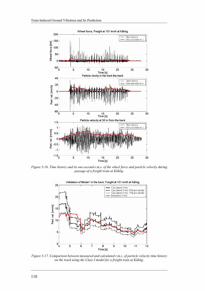
Train-Induced Ground Vibration and Its Prediction
110
Figure 5-16. Time history and its one-second-r.m.s. of the wheel force and particle velocity during
passage of a freight train at Kåhög.
Figure 5-17. Comparison between measured and calculated r.m.s. of particle velocity time history
on the track using the Class I model for a freight train at Kåhög.

Mehdi Bahrekazemi
111
Figure 5-18. Comparison between measured and calculated r.m.s. of particle velocity time history
at 30 m from the centerline of the track using the Class I model for a freight train at Kåhög.
5.3 INTEGRATING THE MODEL WITH A GIS SYSTEM Nowadays Geographical Information System, GIS is used in many projects all over the world. These projects cover many fields such as water resources management, urban planning, and so on. Here GIS is used together with the semi-empirical model for train-induced ground vibrations described earlier in this chapter to present a user friendly and effective tool for studying the environment vibrations from railways.
5.3.1 Definition of GIS According to (Burough &Mcdonnell, 1998) three definitions for GIS can be presented. These three definitions are the Toolbox-based definition, the Database definition, and the Organization based definition. According to the first definition, GIS is an information technology which stores, analyses, and displays both spatial and non spatial data. On the other hand the database definition defines GIS as any manual or computer based set of procedures used to store and manipulate geographically referenced data. At last the organization based definition defines GIS as an automated set of functions that provides professionals with advanced capabilities for the storage, retrieval, manipulation and display of geographically located data. Any geographical information system has three important components which have to be in balance for the system to function satisfactorily. These three components are computer hardware, sets of application software modules, and a proper organizational context including skilled people. The hardware components of a GIS system usually consist of computer with a hard disk drive for storing the programs and data. In order to create more storage
Train-Induced Ground Vibration and Its Prediction
112
capacity, extra storage like digital tape cassettes and optical CD-ROMs can also be used. A digitizer or scanner is used to convert maps and documents into digital forms and a plotter or printer or any other display device is used to present the results of the data processing. Usually many computers are connected to each other through local or global networks which can be optical fiber lines or ordinary telephone lines via a modem. The sets of programs and software used for GIS can be classified into five different categories as listed below: a- Data input and verification b- Data storage and database management c- Data output and presentation d- Data transformation e- Interaction with the user As the requirements of users to retrieve and transform data are unlimited, most systems provide a range of interfaces by which the user can interact with the system. One such way is through typing in simple commands via a command language interpreter (CLI). Users can write a set of commands in a file that can carry out well-defined operations by linking several modular commands together without any need for the user to be a skilled computer programmer. Sometimes the GIS is used to prepare the data needed for a complex model that is programmed outside the system using a standard computer language. Once the model has been run, the results are transferred back to the GIS for display. All this would not work efficiently (or at all) if it is not run by skilled people in an appropriate organization. Therefore in order to acquire a good and optimum GIS system, attention must be paid to all the three links described above at the same time.
5.3.2 GIS Software
There are different GIS programs available on the market but the three programs used more commonly are ArcView (or ArcInfo), GeoMedia, and GRASS. While the first two softwares are commercial, the last one can be downloaded freely from the internet. Banverket in Sweden is using Arcview for its projects and the Norwegian geotechnical Institute, NGI is using GeoMedia. The author on the other hand has decided to use GRASS version 5 for this work as it is free and available to him. The Geographic Resource Analysis System (GRASS) is a geographical information system (GIS) that in the beginning was designed and developed by researchers at the U.S. Army Construction Engineering Research Laboratory (USACERL). Today GRASS is supported and enhanced by the GRASS Development Team headquarters at ITC-irs, Trento (Italy) and Baylor University, Waco (U.S.A.) (Neteler et al. 2001). Using software provided by GRASS it is possible to organize, portray, and analyze digital spatial data. GRASS is open source software, which last version; GRASS 5 was released under GNU General Public License (GPL) in October 1999.
Mehdi Bahrekazemi
113
GRASS is a general purpose geographical information system and is intended for users like regional land planners, ecologists, geographers, archeologists, and landscape architects. As yet no GRASS tools exists for the modeling and simulation of traffic. But using the tools already available, the author has shown that it can suitably be used for simulation of ground vibrations due to train traffic. Probably the most positive point about GRASS is that it is free and therefore can be acquired and used without extra costs (it can be downloaded from http://grass.itc.it/download.html). On the other hand the program runs under UNIX operating system that is not the common operating system in many places where GIS is used (for example the Swedish Rail Administration, Banverket uses Arcview on Windows).
5.3.3 ENVIB’s GIS system
In order to develop the GIS system suitable for using together with the semi-empirical model presented earlier in this chapter, the mathematical description of the model is presented in the general form discussed in section 2.1.2. This is presented here by Equation 5-4 for convenience of the reader. Although the semi-empirical model described by Equation 5-3 does not include material damping in an explicit way (the total effect of geometrical and material damping is considered by the attenuation power n), the general form including even material damping is used. In this way the GIS system may be used later with more complex models including the geometrical and material damping separately.
( )0
00
rrn
errvv −−
−
⋅
⋅= α
Equation 5-4
where, =0v Particle velocity at the source that may be determined using Equation 5-1. =0r The distance from the source to the reference point on the ground =r The distance from the source to the receiver =n The power of geometric attenuation (may be adopted from Table 5-1) =α The factor for material damping (must be zero if n is adopted from Table 5-1)
In Figure 5-19 the fictitious geotechnical map of an area of 2000 x 2000 m2 is shown. The raster elements used for this purpose have a size of 2 x 2 m2. This means that the area consists of one million raster elements. The number of elements can be more than one million depending on the size of the map and the raster elements. On the other hand more elements means more running time for the program while larger elements means less accurate results. The designer can chose the appropriate size of the area and raster elements by experience. The figure also shows one possible candidate for the track path that the railway designer might want to choose for preliminary ground vibration investigations. Referring to Equation 5-4 it is seen that the equation can be divided into two parts. The first part, ( ) nrrv −⋅ 00 / is not dependent on the soil material along the path of the waves from the source to the receiver, while the second part ( )0rre −−α includes the material damping factor, α which depends on the soil material along the path. As there may be different types of soil between the track and the

Train-Induced Ground Vibration and Its Prediction
114
receiving point, this should be taken into account when determining the material damping. In order to be able to use Equation 5-4 with the GIS system, some modifications must be done in the form of the equation. Here the second part of the equation which represents material damping is named L, (see Equation 5-5). L can change between one and zero as the waves move from the source to the infinity. The incremental change of L can then be written as given by Equation 5-6.
( )0rreL −−= α Equation 5-5
( ) ( )
−−
−⋅= −− ααα
00 rr
drde
drdL rr Equation 5-6
Within each soil type the term drd /α is equal to zero, while on the borders between two regions with different soils it may be other than zero. On the other hand the whole map of the area is divided into raster elements so that no element is situated on the border. As all the calculations in GIS are performed on a raster element basis, the term drd /α is always zero for each raster element. Therefore the incremental change in L may be written as given by Equation 5-7, while the total effect of material damping along the path is given by Equation 5-8. Finally Equation 5-4 can be rewritten as Equation 5-9 which is ready to be used for raster element based calculations in the GIS system. The GIS system including the computer code prepared for performing the calculations is presented in a separate report to the EnVib project (Bahrekazemi, 2002a).
( ) reL rr ∆⋅⋅−=∆ −− 0αα Equation 5-7
( )∑ ∆⋅⋅−= −− reL rr 01 αα Equation 5-8
Lrrvv
n
⋅
⋅=
−
00
Equation 5-9
Figure 5-19. Fictitious geotechnical map of the area where the railway is going to be built.

Mehdi Bahrekazemi
115
5.3.4 An example of using the model within the GIS system Some intermediate and final results are presented in this section. As it is shown in Figure 5-19 four different types of soil are assumed to exit in this area with different material properties that would result in different vibration levels as the train runs along the track. Running the program prepared for this purpose, the user has the possibility to see how large the vibration is at different locations as the train runs on the imaginary track as shown by Figure 5-20 (left part). At the end of the running time of the program the user can see the map of the maximum particle velocities for the whole area and identify the areas with ground vibration problems as shown in the right part of Figure 5-20.
Figure 5-20. A map showing particle velocity at different points in a small part of the site due to
passage of a train car with four axles (left), and the map of the whole area with a small part to the left that shows the maximum particle velocities expected in different colors (right).
5.4 DISCUSSION AND CONCLUSIONS A semi-empirical model has been presented in this chapter based on measurements from four sites in Sweden. The model results show good agreement with the measurements when validating the model using data that have not been used for determining the model parameters. A set of model parameters are presented for the four different sites for which measurement data have been available. The parameters should be suitable to be used for sites with geotechnical conditions similar to those for the four sites. This is not a very serious limitation for the model as it is very rare to encounter ground-borne vibration problem due to train traffic at sites with very different geotechnical conditions compared to these four sites. As more measurement data becomes available, new sets of parameters may be prepared for sites with different soil conditions. The semi-empirical model can easily be used in the preliminary phase of projects where a new railway is being designed or an existing track is going to be

Train-Induced Ground Vibration and Its Prediction
116
modified. In this way the designer has a powerful tool that helps him to consider many different alternatives in a rather short time and to choose the best one. In those cases that the model suggests a possibility of having problems due to excessive ground-borne vibration, the railway designer may either consider more detailed investigation of the problem area using for example more accurate models or performing measurements at the site or simply choose another route for the railway. In case of railway tracks currently in use, the model can be used together with parameters that are specially determined for different parts of the track, to determine optimum speed for trains with different axel loads. Therefore each freight train can run at a maximum allowable speed determined as a function of its axel load and thereby make maximum advantage of the railway capacity without causing excessive environmental vibration. A GIS system can successfully be used together with the semi-empirical model to predict ground vibration from train traffic along the railway. Although the program GRASS 5 has been used for the example discussed in this chapter, it should be possible to use other programs such as ArcInfo or GeoMedia for the same purpose.
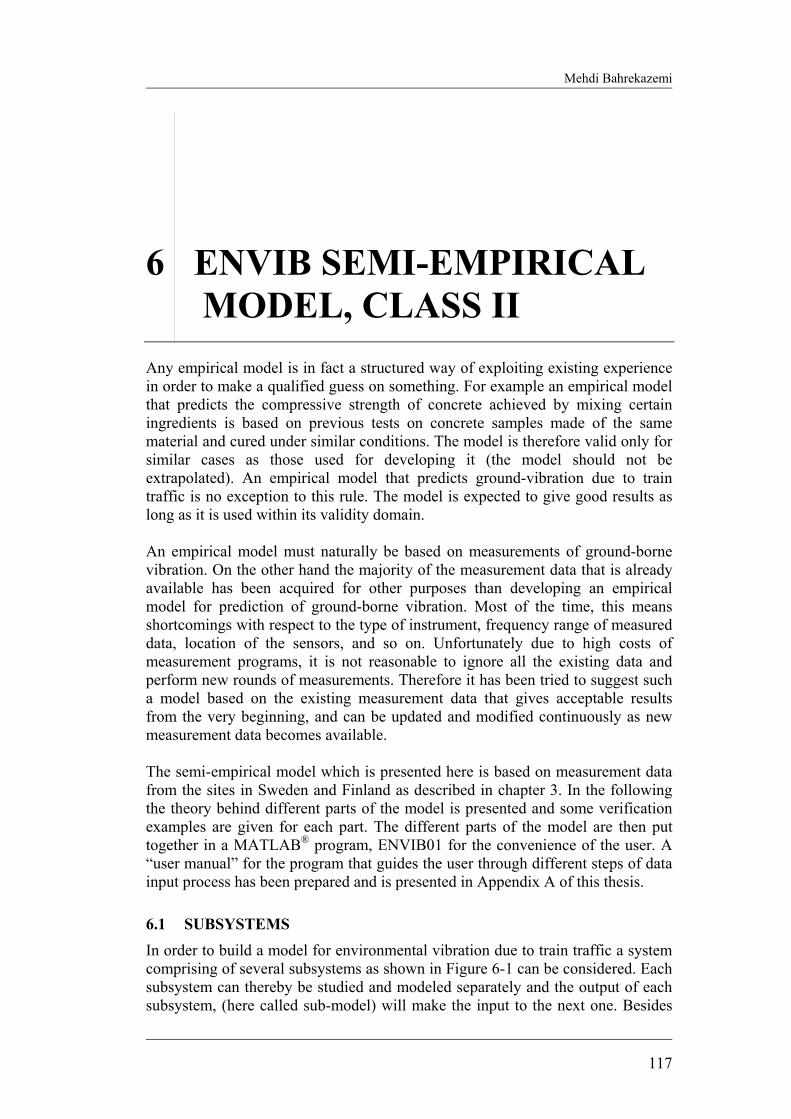
Mehdi Bahrekazemi
117
6 ENVIB SEMI-EMPIRICAL MODEL, CLASS II
Any empirical model is in fact a structured way of exploiting existing experience in order to make a qualified guess on something. For example an empirical model that predicts the compressive strength of concrete achieved by mixing certain ingredients is based on previous tests on concrete samples made of the same material and cured under similar conditions. The model is therefore valid only for similar cases as those used for developing it (the model should not be extrapolated). An empirical model that predicts ground-vibration due to train traffic is no exception to this rule. The model is expected to give good results as long as it is used within its validity domain. An empirical model must naturally be based on measurements of ground-borne vibration. On the other hand the majority of the measurement data that is already available has been acquired for other purposes than developing an empirical model for prediction of ground-borne vibration. Most of the time, this means shortcomings with respect to the type of instrument, frequency range of measured data, location of the sensors, and so on. Unfortunately due to high costs of measurement programs, it is not reasonable to ignore all the existing data and perform new rounds of measurements. Therefore it has been tried to suggest such a model based on the existing measurement data that gives acceptable results from the very beginning, and can be updated and modified continuously as new measurement data becomes available. The semi-empirical model which is presented here is based on measurement data from the sites in Sweden and Finland as described in chapter 3. In the following the theory behind different parts of the model is presented and some verification examples are given for each part. The different parts of the model are then put together in a MATLAB® program, ENVIB01 for the convenience of the user. A “user manual” for the program that guides the user through different steps of data input process has been prepared and is presented in Appendix A of this thesis.
6.1 SUBSYSTEMS In order to build a model for environmental vibration due to train traffic a system comprising of several subsystems as shown in Figure 6-1 can be considered. Each subsystem can thereby be studied and modeled separately and the output of each subsystem, (here called sub-model) will make the input to the next one. Besides
Train-Induced Ground Vibration and Its Prediction
118
the input signal coming from the previous sub-model, some kind of noise may also be considered as shown in figure (v1-v4). This noise can be due to measurement noise or nonlinearities that are not considered by the linear input-output relationship of the sub-model. The ambient vibrations are also considered as noise for this purpose. The first sub-model as shown in Figure 6-1 with the input F and out R1 is presented using system identification techniques for linear systems. Although the sub-model is not perfectly linear as it will be discussed later in this chapter, the experience shows that a linear model of the sub-system is capable of capturing the most important aspects for practical purpose. The second sub-model is based on a transfer function approach that relates vibrations at points R1 and R2 in the near field as shown in Figure 6-1. The third subsystem is modeled using a stochastic approach to the issue. For this sub-model, wave propagation from a source point, through the path to another point on the ground is considered, taking into account the stochastic character of both the source and the path. The forth sub-model is also a transfer function similar to the second sub-model, between a point on the ground and another point inside the building.
rail, pad,sleeper,ballast,
embank & soil
near-field soil path structureF R1 R2 R3 R4
v1 v2 v3 v4
R1 R2 R3
R4
F
Figure 6-1. Dividing the system into subsystems.
Figure 6-2 shows the user interface of the ENVIB01 model based on the sub-models described above. The program that is developed within MATLAB® environment gives the user the possibility of specifying different parts of the model with respect to the case which is being studied. After selecting the type of the train from the train type pop-up menu, the user continues with selecting a track type similar to the one under consideration. The program then computes the time histories of the particle acceleration, velocity, and displacement in the track

Mehdi Bahrekazemi
119
or at a point close to the track. Selecting a path similar to the one being simulated from the pop-up menu, and using the predicted time histories for the track, the particle velocity time history is then predicted for a point on the ground at a specified distance from the track. Sub-model II is automatically chosen based on track and path types. It is also possible for the user to modify the path by filling in the places indicated under the path pop-up menu. The last calculated particle velocity is in its turn used to calculate the particle velocity for a point inside the building after selecting the building type from its pop-up menu. For more detailed information about how the different inputs are given to the program see the “user manual” of the program in Appendix A. Dividing the model in this way and making a library for each sub-model makes it possible to build a user-tailored model by selecting and combining different parts of the model. As more cases of measurements become available in future, the libraries become larger including more items. Another advantage of dividing the model into different sub-models is that it is possible to replace parts of the model with real measurement data from the site in case this is available and thereby acquire more accurate results. For example one can use vibration measurements in the track as input to the next part of the model (sub-model I or sub-model II) to study the effect of vibrations inside a building which will be built at a certain distance from the track. In the rest of this chapter the four different sub-models are discussed presenting the theory behind each of them.
Figure 6-2 User interface of ENVIB01 program.

Train-Induced Ground Vibration and Its Prediction
120
6.1.1 Sub-model I, track The first subsystem shown in Figure 6-1 is the track including the rails, pads, sleeper, ballast, sub-ballast and underlying soil. The input to this subsystem is train load in form of axel or wheel force time history. In this thesis the wheel force is used in the development of the model.
6.1.1.1 Modeling subsystem I There are two different ways of constructing a model of a linear dynamic system. One is called the non-parametric method and includes the study of impulse-response and transfer function estimation of the system. The other one is a specially formulated linear “confection model” which is a parametric model for which the parameters are chosen based on input and output signals. The transfer function approach which is used for subsystem II, and subsystem IV will be discussed later. In case of parametric models on the other hand a special type of model structure including a rather few number of parameters are chosen first and the parameters are then estimated based on input-output signals and some fit criterion. The standard type “confection” models include ARX, ARMAX, OE, and BJ models (see for example Ljung, 1987), that can be presented by the general form as given by Equation 6-1.
))( ,(Η +)(= τθτθ equ ))G(q, y(t) Equation 6-1
where y(t) is the output signal, u(t) is the input signal, and e(t) is white noise. G(q,θ) and H(q,θ) are rational functions defined according to Equation 6-2-Equation 6-4, where q is shift operator and θ is the parameter vector. If F(q), and D(q) are the same, A(q) is used instead of both F(q) and D(q) as in case of ARMAX model.
nfnf
nbnknb
nknk
qfqfqbqbqb
qFqB
−−
+−−−−−
++++++==
...1...
)()()G(q, 1
1
1121θ
Equation 6-2
ndnd
ncnc
qdqdqcqc
qDqC
−−
−−
++++++==
...1...1
)()()H(q, 1
1
11θ Equation 6-3
na
naqaqaqA −− +++= ...1)( 11 Equation 6-4
In Equation 6-2 a shift in time is presented by nk, and the parameter vector θ contains the coefficients bi, ci, di and fi. The model given by Equation 6-5 is called Box-Jenkins (BJ) model and its order is determined by the choice of nb, nc, nd, nf and nk. By choosing different combinations of nb, nc, nd, nf and nk other models are obtained as defined by the following equations:
BJ: )()()()(
)()()( te
qDqCtu
qFqBty +=
Equation 6-5

Mehdi Bahrekazemi
121
ARMAX: )()()()(
)()()( te
qAqCtu
qAqBty +=
Equation 6-6
ARX: )()(
1)()()()( te
qAtu
qAqBty +=
Equation 6-7
OE: )()()()()( tetu
qAqBty +=
Equation 6-8
Now appropriate choices must be made for the parameters ai, bi, ci, di and fi inθ. The main idea is to compare the predicted output with the measured output and minimize the error criterion. If the predicted output is shown by ŷ(t|θ) then the error can be given according to Equation 6-9.
)|()(),( θθε tytyt −= Equation 6-9
The sum of these errors for all time increments gives the error criterion that must be minimized in order to findθ.
)t,(1)(1
2 θεθ ∑=
= N
tN N
V Equation 6-10
In practice there are computer programs that perform the calculations and can easily be used to find the best model after the user has decided on the type of the model. For the model presented in this thesis, the System Identification Toolbox provided by MATLAB® (SITB) has been used to determine the model parameters.
6.1.1.2 Some examples Figure 6-3 shows the time histories of wheel force and particle acceleration at 3.5 m from the track centerline for an X2000 train driving at 132 km/h towards east at Kåhög (ID309). As it is seen from Figure 6-4 the coherence function between the measured wheel force and particle acceleration shows a somewhat linear relationship for most frequencies up to 100Hz. The coherence is about 0.7 on average for frequencies up to 100Hz. Coherence less than unity at many frequencies may be explained by existence of noise in the signals as well as nonlinearities. Figure 6-5 shows a comparison between the measured and calculated particle acceleration for a point at 3.5 m from the track centerline. The model used for this simulation is a narrow band model comprising of five OE models each one for a certain frequency band (where the name narrow band model comes from). In Figure 6-6 it is seen that the predicted acceleration agrees with the measured data up to about 100 Hz. In general the agreement between calculation and measurement is good in the most important part of the signal that carries the

Train-Induced Ground Vibration and Its Prediction
122
major part of the vibrational energy. Bad agreement between the measurement and calculation at high frequencies may be due to the noise in the measurement.
Figure 6-3. Time histories of wheel force (ch1) and particle acceleration (ch6) at 3.5m from the
track centerline for an X2000 at 132km/h towards east at Kåhög (ID309).
Figure 6-4. Coherence function between ch1 and ch6 for ID 309, showing approximate linearity
up to 100 HZ.
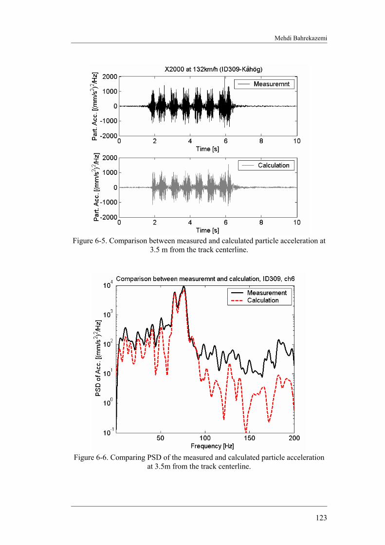
Mehdi Bahrekazemi
123
Figure 6-5. Comparison between measured and calculated particle acceleration at
3.5 m from the track centerline.
Figure 6-6. Comparing PSD of the measured and calculated particle acceleration
at 3.5m from the track centerline.

Train-Induced Ground Vibration and Its Prediction
124
6.1.2 Sub-model II, near field The second sub-model as shown in Figure 6-1 is needed in order to take into account the near-filed effect close to the track. Measurement data from different sites show that the frequency character of vibration changes when two points, one close to the track and the other one at some distance (about 10 m) from the track are compared. This change can not be explained by simple geometrical and material damping. Therefore there must be some kind of transfer function that takes this issue into account.
For a linear system without extraneous noise the frequency response function is calculated using Equation 6-11, where Guv(f) is the cross-spectrum function of the input and output signal and Guu(f) is the autospectrum function of the input signal. If the system is not linear or if there is extraneous noise as shown in Figure 6-7, where m(t) and n(t) are some kind of noise, the application of Equation 6-11 will give only a linear approximation of the system response characteristics. Nevertheless the result will be the best possible linear approximation in the least-square sense of the frequency response function for the specified input conditions. This implies that for systems that behave nonlinearly the natural input signals should be used for determination of the frequency response function (Bendat, 1993).
)()()(
fGfGfH
uu
uv= Equation 6-11
The transfer function representing sub-model II has been obtained using available measurement data. Because of the stochastic character of the vibrations, the transfer function has been calculated as the average of several transfer functions based on different train passages. A comparison between the measured and calculated particle velocity time histories at 7.5 m from the track centerline is shown in Figure 6-8. It is seen from the figure that the time history obtained from the average transfer function has good agreement with the measured one.
H(f) Σ
n(t)
x(t)
v(t)y(t)
Σ
u(t)
m(t)
Figure 6-7. Single input-single output system with input and output noise.
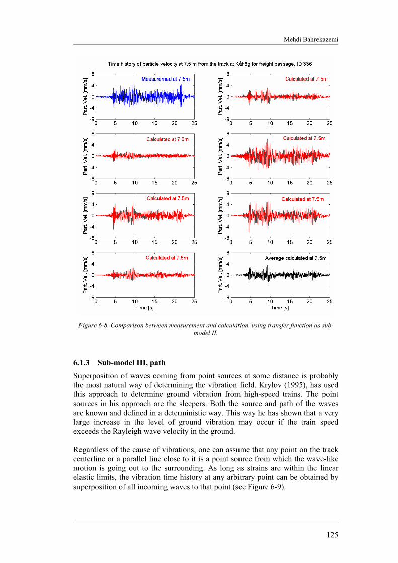
Mehdi Bahrekazemi
125
Figure 6-8. Comparison between measurement and calculation, using transfer function as sub-
model II.
6.1.3 Sub-model III, path
Superposition of waves coming from point sources at some distance is probably the most natural way of determining the vibration field. Krylov (1995), has used this approach to determine ground vibration from high-speed trains. The point sources in his approach are the sleepers. Both the source and path of the waves are known and defined in a deterministic way. This way he has shown that a very large increase in the level of ground vibration may occur if the train speed exceeds the Rayleigh wave velocity in the ground. Regardless of the cause of vibrations, one can assume that any point on the track centerline or a parallel line close to it is a point source from which the wave-like motion is going out to the surrounding. As long as strains are within the linear elastic limits, the vibration time history at any arbitrary point can be obtained by superposition of all incoming waves to that point (see Figure 6-9).
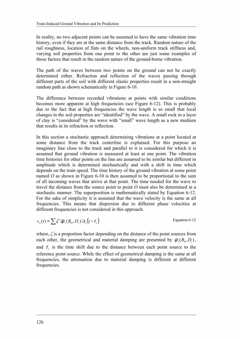
Train-Induced Ground Vibration and Its Prediction
126
In reality, no two adjacent points can be assumed to have the same vibration time history, even if they are at the same distance from the track. Random nature of the rail roughness, location of flats on the wheels, non-uniform track stiffness and, varying soil properties from one point to the other are just some examples of those factors that result in the random nature of the ground-borne vibration. The path of the waves between two points on the ground can not be exactly determined either. Refraction and reflection of the waves passing through different parts of the soil with different elastic properties result in a non-straight random path as shown schematically in Figure 6-10. The difference between recorded vibrations at points with similar conditions becomes more apparent at high frequencies (see Figure 6-12). This is probably due to the fact that at high frequencies the wave length is so small that local changes in the soil properties are “identified” by the wave. A small rock in a layer of clay is “considered” by the wave with “small” wave length as a new medium that results in its refraction or reflection. In this section a stochastic approach determining vibrations at a point located at some distance from the track centerline is explained. For this purpose an imaginary line close to the track and parallel to it is considered for which it is assumed that ground vibration is measured at least at one point. The vibration time histories for other points on the line are assumed to be similar but different in amplitude which is determined stochastically and with a shift in time which depends on the train speed. The time history of the ground vibration at some point named O as shown in Figure 6-10 is then assumed to be proportional to the sum of all incoming waves that arrive at that point. The time needed for the wave to travel the distance from the source point to point O must also be determined in a stochastic manner. The superposition is mathematically stated by Equation 6-12. For the sake of simplicity it is assumed that the wave velocity is the same at all frequencies. This means that dispersion due to different phase velocities at different frequencies is not considered in this approach.
( )∑ −⋅⋅= iiiio tvDRtv τψζ ),()( 0 Equation 6-12
where, ζ is a proportion factor depending on the distance of the point sources from each other, the geometrical and material damping are presented by ),( 0 ii DRψ , and iτ is the time shift due to the distance between each point source to the reference point source. While the effect of geometrical damping is the same at all frequencies, the attenuation due to material damping is different at different frequencies.
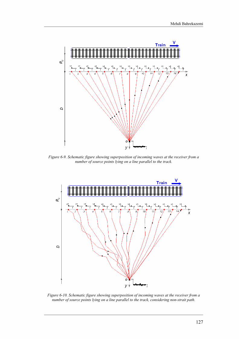
Mehdi Bahrekazemi
127
Figure 6-9. Schematic figure showing superposition of incoming waves at the receiver from a
number of source points lying on a line parallel to the track.
Figure 6-10. Schematic figure showing superposition of incoming waves at the receiver from a
number of source points lying on a line parallel to the track, considering non-strait path.
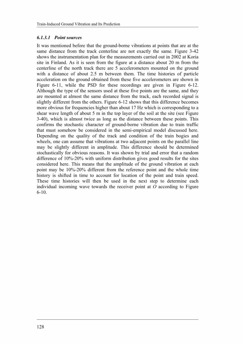
Train-Induced Ground Vibration and Its Prediction
128
6.1.3.1 Point sources It was mentioned before that the ground-borne vibrations at points that are at the same distance from the track centerline are not exactly the same. Figure 3-42 shows the instrumentation plan for the measurements carried out in 2002 at Koria site in Finland. As it is seen from the figure at a distance about 20 m from the centerline of the north track there are 5 accelerometers mounted on the ground with a distance of about 2.5 m between them. The time histories of particle acceleration on the ground obtained from these five accelerometers are shown in Figure 6-11, while the PSD for these recordings are given in Figure 6-12. Although the type of the sensors used at these five points are the same, and they are mounted at almost the same distance from the track, each recorded signal is slightly different from the others. Figure 6-12 shows that this difference becomes more obvious for frequencies higher than about 17 Hz which is corresponding to a shear wave length of about 5 m in the top layer of the soil at the site (see Figure 3-40), which is almost twice as long as the distance between these points. This confirms the stochastic character of ground-borne vibration due to train traffic that must somehow be considered in the semi-empirical model discussed here. Depending on the quality of the track and condition of the train bogies and wheels, one can assume that vibrations at two adjacent points on the parallel line may be slightly different in amplitude. This difference should be determined stochastically for obvious reasons. It was shown by trial and error that a random difference of 10%-20% with uniform distribution gives good results for the sites considered here. This means that the amplitude of the ground vibration at each point may be 10%-20% different from the reference point and the whole time history is shifted in time to account for location of the point and train speed. These time histories will then be used in the next step to determine each individual incoming wave towards the receiver point at O according to Figure 6-10.
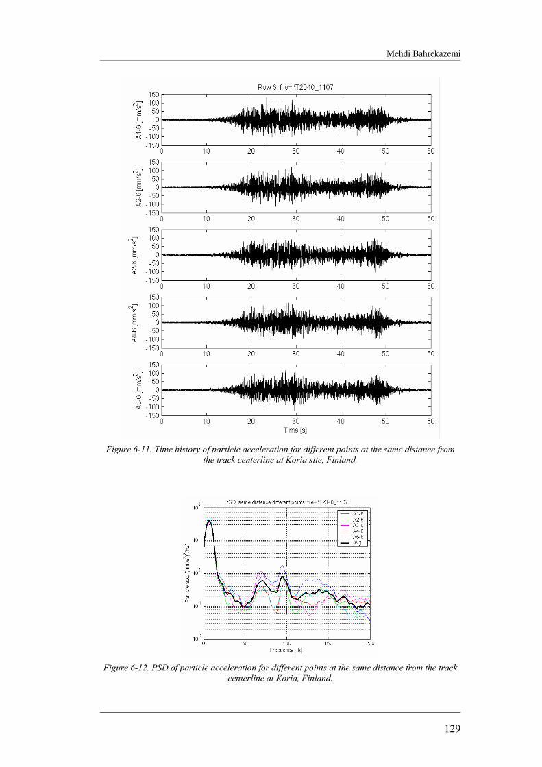
Mehdi Bahrekazemi
129
Figure 6-11. Time history of particle acceleration for different points at the same distance from
the track centerline at Koria site, Finland.
Figure 6-12. PSD of particle acceleration for different points at the same distance from the track
centerline at Koria, Finland.

Train-Induced Ground Vibration and Its Prediction
130
6.1.3.2 Gamma distribution of the path length As discussed earlier in this section one reason behind the stochastic nature of ground-borne vibration due to train traffic is the path from the “source” to the receiver. Due to inhomogeneities in the soil, the waves travel in very complicated paths as they are reflected and refracted at the borders between different materials. One effective way of considering this issue is to determine the length of the path of waves from the source to the receiver in a stochastic way. The probability density function used to describe the distribution of path length is the key issue with this respect. This function determines how much of the energy of the waves will reach the receiver at any time. A distribution function which is narrow means that the medium from the point sources to the receiver is more like a homogeneous half space. On the other hand a wide distribution curve with large standard deviation means that the medium is highly inhomogeneous resulting in very different path for the energy coming from different point sources as shown in Figure 6-10. A gamma distribution has a probability density function defined by Equation 6-13 (Benjamin& Cornell, 1970) with parameters v and k, where Γ(k) is a value of the gamma function defined by Equation 6-14. In the special case when k=1, the exponential distribution is obtained, which has a probability density function similar to the one shown in the left part of Figure 6-13. The gamma distribution gives the possibility of concentrating the path distances around a certain mean and with a certain variance, by choosing appropriate parameters.
)()()(
1
kevxvxf
vxk
x Γ=
−−
; 0≥x Equation 6-13
∫∞
−−=Γ0
1)( dxexk xk Equation 6-14
It can be shown that a value from a general gamma distribution with parameters v and k may be generated using Equation 6-15 in which u1, u2, and u3 are values generated from the standard uniform distribution, provided that 1)1/(1
2/1
1 ≤+ −kk uu , and 1´≥k is the integer part of k. Using Equation 6-15, a total of (k´+3) uniformly distributed numbers must be generated first in order to obtain one gamma distributed random number.
( ) )1/(12
/11
/11
3'
43ln1ln1
kk
kk
ii uu
uu
vu
vx −
+
= +−+−= ∑
Equation 6-15
The above procedure is integrated into a simple MATALB program that produces an arbitrary amount of gamma distributed random numbers. Figure 6-13 shows the distribution of two example sets of 1000 gamma distributed random numbers between zero and one. The shape of the distribution should be chosen with respect to the soil layering at the site. In practice different shapes can be tried in order to

Mehdi Bahrekazemi
131
find the best fit to the measurement data. This distribution is used here in order to estimate the travel time from each source point to the receiver. The wave from each point source is then shifted in time accordingly to obtain the undamped wave that would have reached the receiver if no damping was involved.
6.1.3.3 Geometrical and material damping
The geometrical and material damping of the waves leaving the point source towards the receiver (accelerometer or geophone on the ground at some distance) are two important issues that must be considered before waves from point sources are superposed. These two different kinds of damping are considered separately. The geometrical attenuation discussed in section 2.1.2 is rewritten here as given by Equation 6-16.
n
rrvv
−
=
0
101
Equation 6-16
where v0 is the vibration amplitude at the first point (the “source point” on a parallel line close to the track) which is at distance r0 from the track centerline, v1 is the vibration amplitude at the receiver which is at distance r1 from the track centerline, and n is geometric damping power which depends on the type of the wave. This dependence is shown in Figure 2-6 for different wave types. In practice the effect of geometrical damping and ζ as stated by Equation 6-12 is combined together in a single factor. The material damping which was given by Equation 2-2 is rewritten as given by Equation 6-17. Putting v1 obtained from Equation 6-16 into this equation, v2 is calculated.
−−
⋅= crrf
evv01)2(
12
πξ
Equation 6-17
Figure 6-13. Two example of gamma distribution with different parameters (the left one, v=1,
k=1.8 and the right one, v=1, k=0.9).
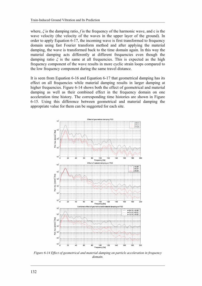
Train-Induced Ground Vibration and Its Prediction
132
where, ξ is the damping ratio, f is the frequency of the harmonic wave, and c is the wave velocity (the velocity of the waves in the upper layer of the ground). In order to apply Equation 6-17, the incoming wave is first transformed to frequency domain using fast Fourier transform method and after applying the material damping, the wave is transformed back to the time domain again. In this way the material damping acts differently at different frequencies even though the damping ratio ξ is the same at all frequencies. This is expected as the high frequency component of the wave results in more cyclic strain loops compared to the low frequency component during the same travel distance. It is seen from Equation 6-16 and Equation 6-17 that geometrical damping has its effect on all frequencies while material damping results in larger damping at higher frequencies. Figure 6-14 shows both the effect of geometrical and material damping as well as their combined effect in the frequency domain on one acceleration time history. The corresponding time histories are shown in Figure 6-15. Using this difference between geometrical and material damping the appropriate value for them can be suggested for each site.
Figure 6-14 Effect of geometrical and material damping on particle acceleration in frequency
domain.

Mehdi Bahrekazemi
133
Figure 6-15. Effect of geometrical and material damping in time domain.
Figure 6-16. Comparison between deterministic and stochastic estimation of vibrations.
At the end of this section a comparison has been made between the results obtained by the stochastic method and those obtained from a deterministic approach. Figure 6-16 shows that especially at low frequencies up to about 10 Hz the effect of stochastic approach is very important.

Train-Induced Ground Vibration and Its Prediction
134
6.1.3.4 Some examples of suitable damping parameters In this section the simulation results obtained from sub-model III is presented for several sites for which measurement data are available.
6.1.3.4.1 Koria site Four simulation results as well as measurement of particle acceleration at a point about 19 m from the track centerline at Koria site are presented in Figure 6-17. It is seen from the figure that the results are slightly different as expected due to the stochastic nature of the model. Therefore in using the model one should repeat the calculation several times and report the average results as well as standard deviation. In Figure 6-18 a comparison between one-second-r.m.s. of ten sample results with that of measured data is presented. Comparison between the simulation results and measurement in the frequency domain is presented in Figure 6-19. The figure shows the result obtained from two different simulation output populations. Although the individual members have a noticeable variation, the average curves are very similar in both cases and show good agreement with the measurement result. These simulation results are obtained for 10 samples in each group of results. Comparison between measurement and simulation result shows that a ζ factor (see Equation 6-12) would be necessary to calibrate the simulation results according to measurements. This ζ could be obtained comparing for example the maximum of the measured r.m.s. with the simulated one. For the present case this would result in a ζ factor of about 0.87 (for geometrical damping power chosen as being 2.0).
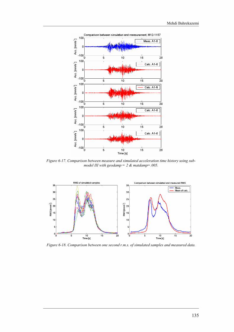
Mehdi Bahrekazemi
135
Figure 6-17. Comparison between measure and simulated acceleration time history using sub-
model III with geodamp = 2 & matdamp=.005.
Figure 6-18. Comparison between one second r.m.s. of simulated samples and measured data.
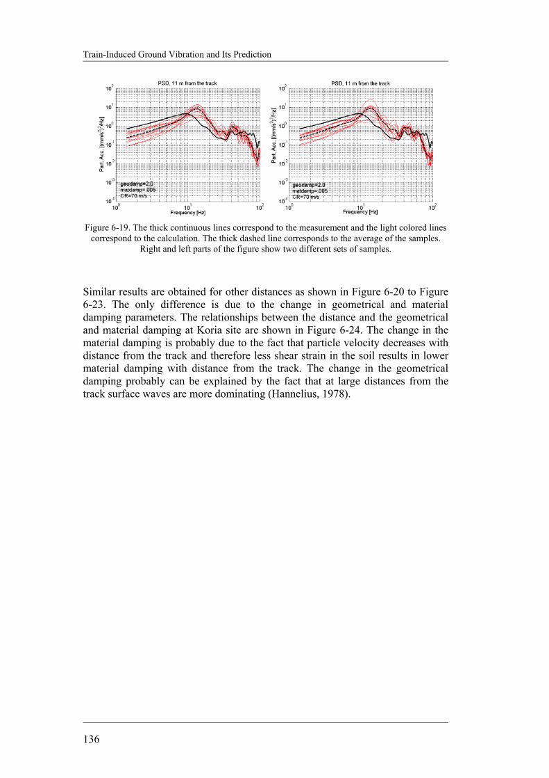
Train-Induced Ground Vibration and Its Prediction
136
Figure 6-19. The thick continuous lines correspond to the measurement and the light colored lines
correspond to the calculation. The thick dashed line corresponds to the average of the samples. Right and left parts of the figure show two different sets of samples.
Similar results are obtained for other distances as shown in Figure 6-20 to Figure 6-23. The only difference is due to the change in geometrical and material damping parameters. The relationships between the distance and the geometrical and material damping at Koria site are shown in Figure 6-24. The change in the material damping is probably due to the fact that particle velocity decreases with distance from the track and therefore less shear strain in the soil results in lower material damping with distance from the track. The change in the geometrical damping probably can be explained by the fact that at large distances from the track surface waves are more dominating (Hannelius, 1978).
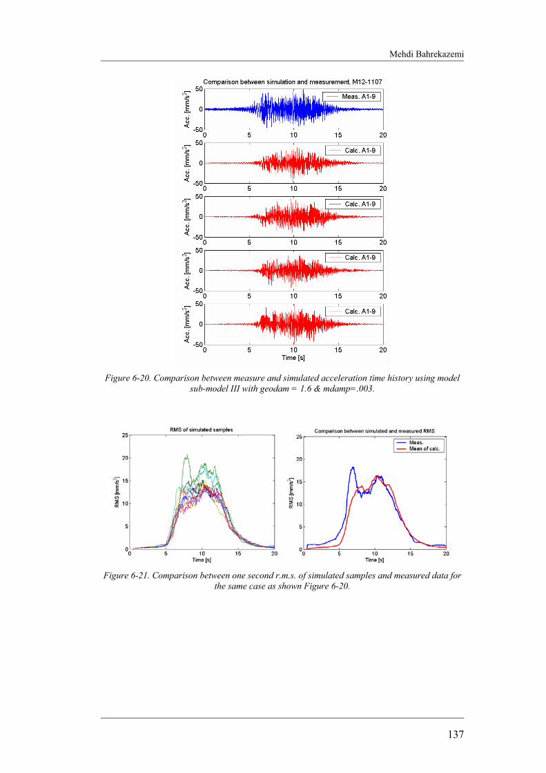
Mehdi Bahrekazemi
137
Figure 6-20. Comparison between measure and simulated acceleration time history using model
sub-model III with geodam = 1.6 & mdamp=.003.
Figure 6-21. Comparison between one second r.m.s. of simulated samples and measured data for
the same case as shown Figure 6-20.
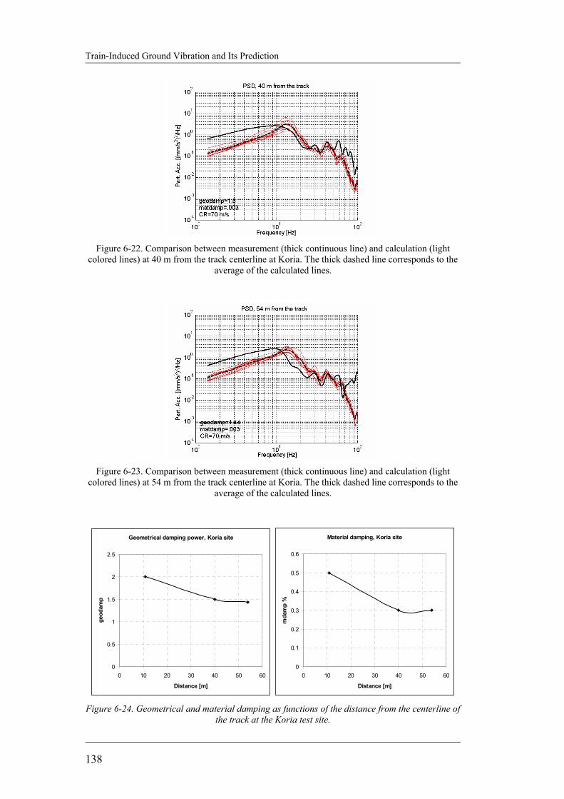
Train-Induced Ground Vibration and Its Prediction
138
Figure 6-22. Comparison between measurement (thick continuous line) and calculation (light
colored lines) at 40 m from the track centerline at Koria. The thick dashed line corresponds to the average of the calculated lines.
Figure 6-23. Comparison between measurement (thick continuous line) and calculation (light
colored lines) at 54 m from the track centerline at Koria. The thick dashed line corresponds to the average of the calculated lines.
Geometrical damping power, Koria site
0
0.5
1
1.5
2
2.5
0 10 20 30 40 50 60
Distance [m]
geod
amp
Material damping, Koria site
0
0.1
0.2
0.3
0.4
0.5
0.6
0 10 20 30 40 50 60
Distance [m]
mda
mp
%
Figure 6-24. Geometrical and material damping as functions of the distance from the centerline of
the track at the Koria test site.
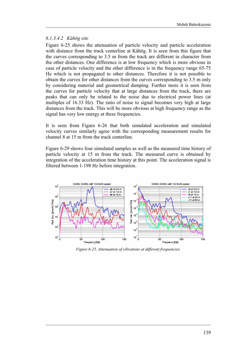
Mehdi Bahrekazemi
139
6.1.3.4.2 Kåhög site Figure 6-25 shows the attenuation of particle velocity and particle acceleration with distance from the track centerline at Kåhög. It is seen from this figure that the curves corresponding to 3.5 m from the track are different in character from the other distances. One difference is at low frequency which is more obvious in case of particle velocity and the other difference is in the frequency range 65-75 Hz which is not propagated to other distances. Therefore it is not possible to obtain the curves for other distances from the curves corresponding to 3.5 m only by considering material and geometrical damping. Further more it is seen from the curves for particle velocity that at large distances from the track, there are peaks that can only be related to the noise due to electrical power lines (at multiples of 16.33 Hz). The ratio of noise to signal becomes very high at large distances from the track. This will be more obvious at high frequency range as the signal has very low energy at these frequencies. It is seen from Figure 6-26 that both simulated acceleration and simulated velocity curves similarly agree with the corresponding measurement results for channel 8 at 15 m from the track centerline. Figure 6-29 shows four simulated samples as well as the measured time history of particle velocity at 15 m from the track. The measured curve is obtained by integration of the acceleration time history at this point. The acceleration signal is filtered between 1-198 Hz before integration.
Figure 6-25. Attenuation of vibrations at different frequencies.

Train-Induced Ground Vibration and Its Prediction
140
Figure 6-26. Comparison between measurement (thick continuous) and average of 10 simulations (thick dashed line) at 15 m from the track centerline at Kåhög. The simulation is based on a point
at 7.5 m from the track.
Figure 6-27. Comparison between measurement (thick continuous) and average of 10 simulations (thick dashed line) at 30 m from the track centerline at Kåhög. The simulation is based on a point
at 7.5 m from the track.
Figure 6-28. Comparison between measurement (thick continuous) and average of 10 simulations (thick dashed line) at 60 m from the track centerline at Kåhög. The simulation is based on a point
at 7.5 m from the track.
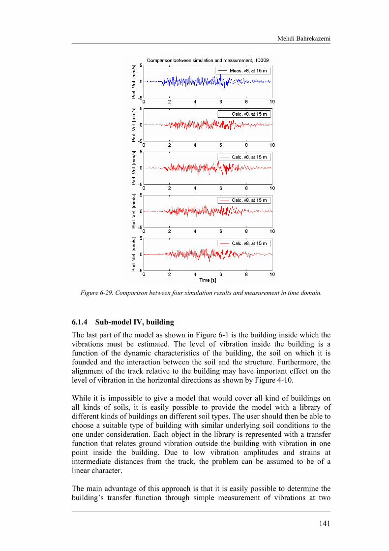
Mehdi Bahrekazemi
141
Figure 6-29. Comparison between four simulation results and measurement in time domain.
6.1.4 Sub-model IV, building The last part of the model as shown in Figure 6-1 is the building inside which the vibrations must be estimated. The level of vibration inside the building is a function of the dynamic characteristics of the building, the soil on which it is founded and the interaction between the soil and the structure. Furthermore, the alignment of the track relative to the building may have important effect on the level of vibration in the horizontal directions as shown by Figure 4-10. While it is impossible to give a model that would cover all kind of buildings on all kinds of soils, it is easily possible to provide the model with a library of different kinds of buildings on different soil types. The user should then be able to choose a suitable type of building with similar underlying soil conditions to the one under consideration. Each object in the library is represented with a transfer function that relates ground vibration outside the building with vibration in one point inside the building. Due to low vibration amplitudes and strains at intermediate distances from the track, the problem can be assumed to be of a linear character. The main advantage of this approach is that it is easily possible to determine the building’s transfer function through simple measurement of vibrations at two
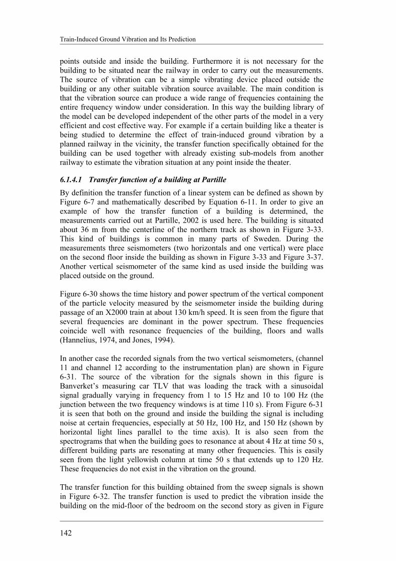
Train-Induced Ground Vibration and Its Prediction
142
points outside and inside the building. Furthermore it is not necessary for the building to be situated near the railway in order to carry out the measurements. The source of vibration can be a simple vibrating device placed outside the building or any other suitable vibration source available. The main condition is that the vibration source can produce a wide range of frequencies containing the entire frequency window under consideration. In this way the building library of the model can be developed independent of the other parts of the model in a very efficient and cost effective way. For example if a certain building like a theater is being studied to determine the effect of train-induced ground vibration by a planned railway in the vicinity, the transfer function specifically obtained for the building can be used together with already existing sub-models from another railway to estimate the vibration situation at any point inside the theater.
6.1.4.1 Transfer function of a building at Partille By definition the transfer function of a linear system can be defined as shown by Figure 6-7 and mathematically described by Equation 6-11. In order to give an example of how the transfer function of a building is determined, the measurements carried out at Partille, 2002 is used here. The building is situated about 36 m from the centerline of the northern track as shown in Figure 3-33. This kind of buildings is common in many parts of Sweden. During the measurements three seismometers (two horizontals and one vertical) were place on the second floor inside the building as shown in Figure 3-33 and Figure 3-37. Another vertical seismometer of the same kind as used inside the building was placed outside on the ground. Figure 6-30 shows the time history and power spectrum of the vertical component of the particle velocity measured by the seismometer inside the building during passage of an X2000 train at about 130 km/h speed. It is seen from the figure that several frequencies are dominant in the power spectrum. These frequencies coincide well with resonance frequencies of the building, floors and walls (Hannelius, 1974, and Jones, 1994). In another case the recorded signals from the two vertical seismometers, (channel 11 and channel 12 according to the instrumentation plan) are shown in Figure 6-31. The source of the vibration for the signals shown in this figure is Banverket’s measuring car TLV that was loading the track with a sinusoidal signal gradually varying in frequency from 1 to 15 Hz and 10 to 100 Hz (the junction between the two frequency windows is at time 110 s). From Figure 6-31 it is seen that both on the ground and inside the building the signal is including noise at certain frequencies, especially at 50 Hz, 100 Hz, and 150 Hz (shown by horizontal light lines parallel to the time axis). It is also seen from the spectrograms that when the building goes to resonance at about 4 Hz at time 50 s, different building parts are resonating at many other frequencies. This is easily seen from the light yellowish column at time 50 s that extends up to 120 Hz. These frequencies do not exist in the vibration on the ground. The transfer function for this building obtained from the sweep signals is shown in Figure 6-32. The transfer function is used to predict the vibration inside the building on the mid-floor of the bedroom on the second story as given in Figure
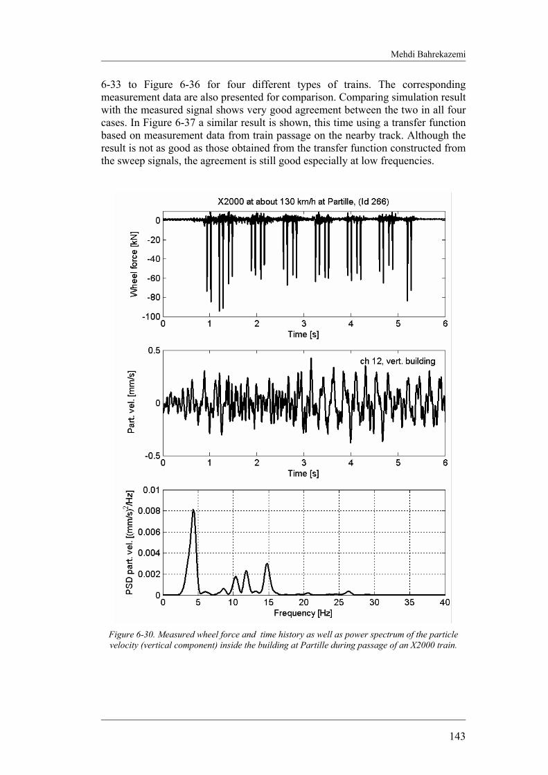
Mehdi Bahrekazemi
143
6-33 to Figure 6-36 for four different types of trains. The corresponding measurement data are also presented for comparison. Comparing simulation result with the measured signal shows very good agreement between the two in all four cases. In Figure 6-37 a similar result is shown, this time using a transfer function based on measurement data from train passage on the nearby track. Although the result is not as good as those obtained from the transfer function constructed from the sweep signals, the agreement is still good especially at low frequencies.
Figure 6-30. Measured wheel force and time history as well as power spectrum of the particle velocity (vertical component) inside the building at Partille during passage of an X2000 train.

Train-Induced Ground Vibration and Its Prediction
144
Figure 6-32. Absolute value of the transfer function between Ch. 11 and Ch. 12 obtained from
sweep sinus signal at Partille.
Figure 6-31. Vertical particle velocity on the ground and inside the building at Partille in time and
frequency domain. The red part of the curves correspond to low frequencies (bellow 15 Hz).
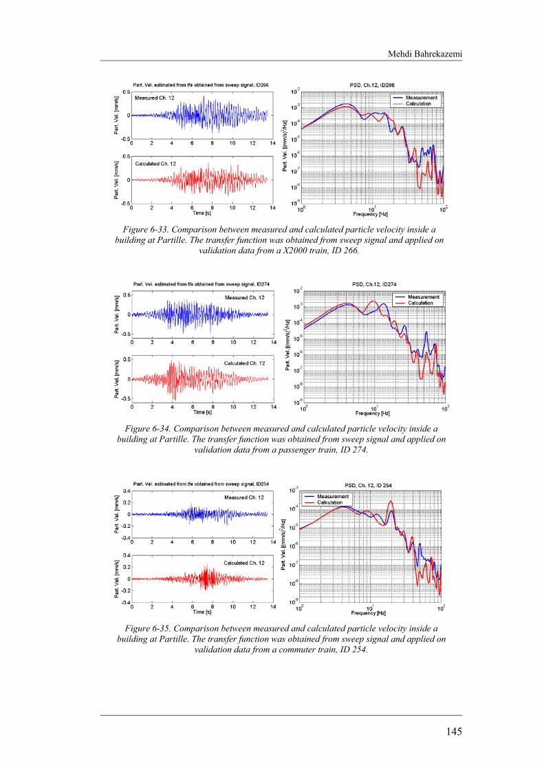
Mehdi Bahrekazemi
145
Figure 6-33. Comparison between measured and calculated particle velocity inside a
building at Partille. The transfer function was obtained from sweep signal and applied on validation data from a X2000 train, ID 266.
Figure 6-34. Comparison between measured and calculated particle velocity inside a building at Partille. The transfer function was obtained from sweep signal and applied on
validation data from a passenger train, ID 274.
Figure 6-35. Comparison between measured and calculated particle velocity inside a
building at Partille. The transfer function was obtained from sweep signal and applied on validation data from a commuter train, ID 254.

Train-Induced Ground Vibration and Its Prediction
146
6.2 VERIFICATION OF THE MODEL
Figure 6-38 shows the simulation result obtained from ENVIB-01 model for an X2000 train passing at 123 km/h. The particle acceleration in the track corresponds to the accelerometer at 3.5 m from the track centerline. Particle velocity time histories for a point on the ground at 36 m from the track centerline as well as a point inside the building using the transfer function for the building at Partille test site are also presented. Corresponding measurement data from this site for are shown in Figure 6-39. As it is seen from these two figures the agreement between the calculated and measured time histories is good. Similar comparison between calculation and measurement for the test site at Kåhög is presented by Figure 6-40 and Figure 6-41. A comparison between the time histories of measured and calculated acceleration in the track (at 3.5 m from the centerline) shows good agreement. The particle velocity time histories in the ground at 30 m from the centerline show good agreement too.
Figure 6-36. Comparison between measured and calculated particle velocity inside a building
at Partille. The transfer function was obtained from sweep signal and applied on validation data from a Freight train, ID 227.
Figure 6-37. Comparison between measured and calculated particle velocity inside a building at Partille. The transfer function was obtained from ID 266 and applied on
validation data from ID 277.
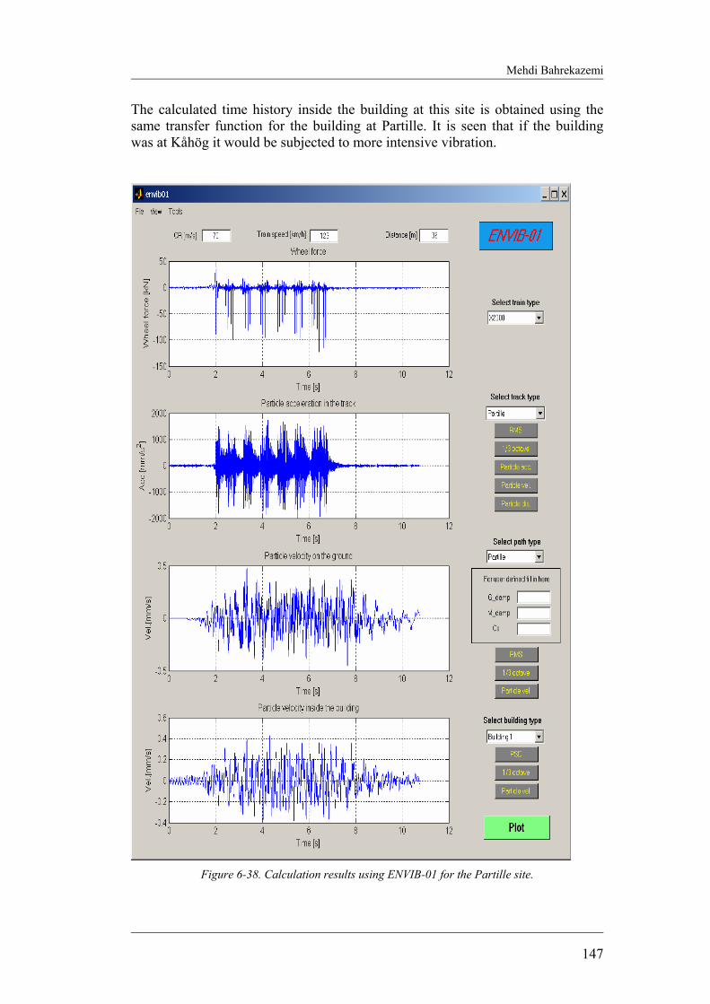
Mehdi Bahrekazemi
147
The calculated time history inside the building at this site is obtained using the same transfer function for the building at Partille. It is seen that if the building was at Kåhög it would be subjected to more intensive vibration.
Figure 6-38. Calculation results using ENVIB-01 for the Partille site.

Train-Induced Ground Vibration and Its Prediction
148
Figure 6-39. Measurement data from the test site at Partille for an X2000 passing the site at about
123 km/h.
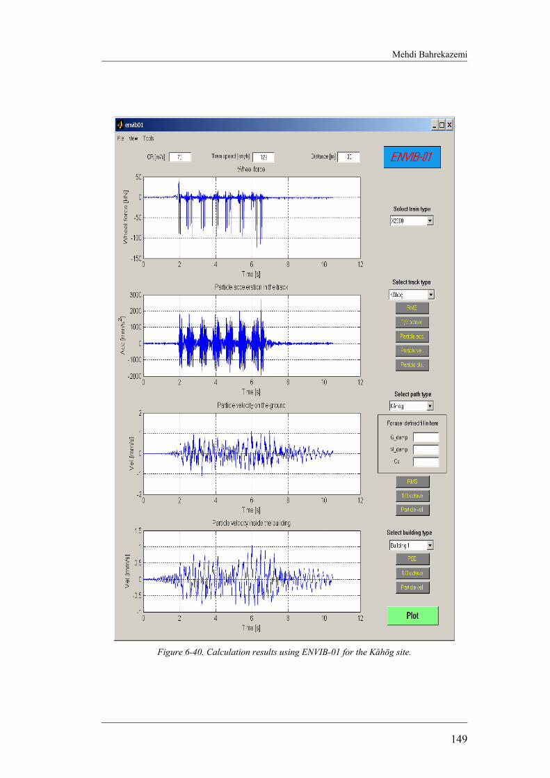
Mehdi Bahrekazemi
149
Figure 6-40. Calculation results using ENVIB-01 for the Kåhög site.
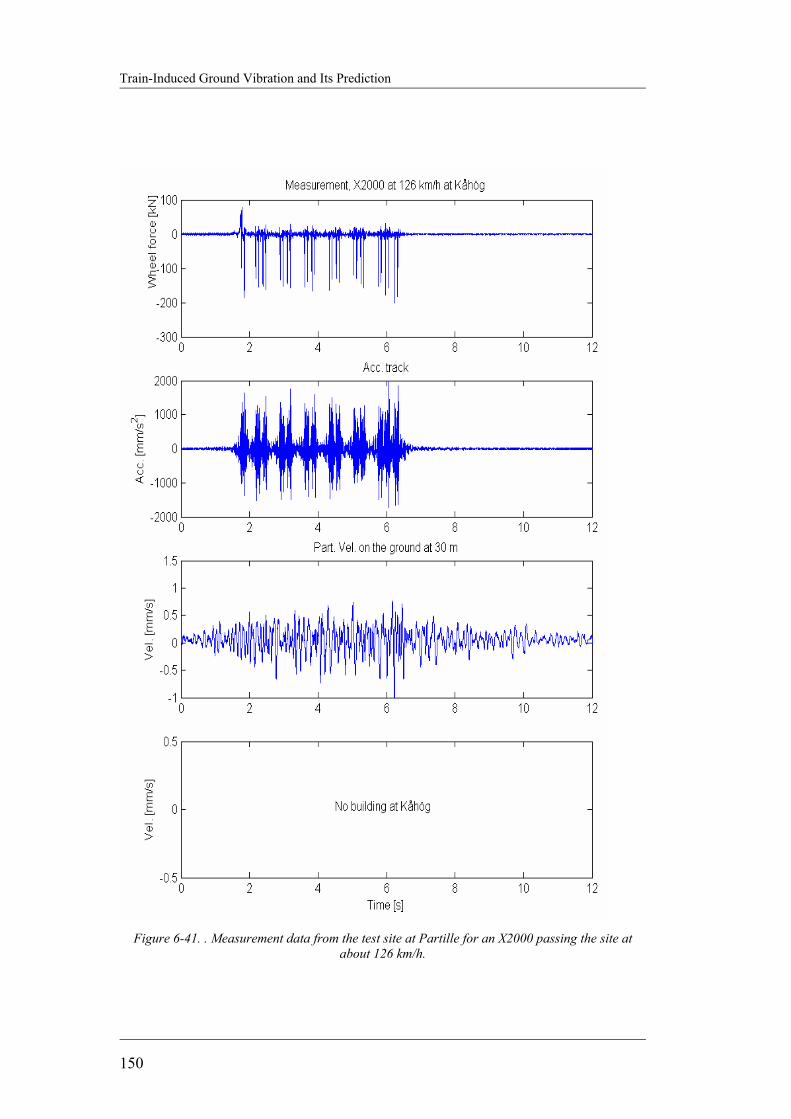
Train-Induced Ground Vibration and Its Prediction
150
Figure 6-41. . Measurement data from the test site at Partille for an X2000 passing the site at
about 126 km/h.
Mehdi Bahrekazemi
151
6.3 DISCUSSION It was shown that by dividing the model into four different sub-models it is possible to simulate the ground-borne vibration due to train traffic. Comparison between calculated and measured vibration time histories shows good agreement between them. By dividing the model into sub-models it is possible to replace some parts of the model with measurement data from the site if available. For example if a new railway is being designed close to a building, the transfer function of the building can be determined by direct measurement using a suitable vibration source. Thereby a prediction with good accuracy can be made on the effect of the planed railway on the building. The same is true if a building is planed to be built close to an existing railway. This time the sub-model corresponding to a similar building may be used together with measurement data from the railway site to predict the vibration situation in the building when it is built. This way decisions can be made on necessary countermeasures at early phase of the building design. The model is user-friendly and little time is needed for its preparation and run (a few minutes). This is an important advantage that gives the designer the possibility of considering many design alternatives in a rather short time. Model results are calculated in a stochastic way. Therefore the calculations should be repeated several times and the average and standard deviation of the results instead of individual result samples be used for evaluation of the situation of ground-borne vibration at the site. The material and geometrical damping is shown to be different at different distances from the track. The change in the material damping is probably due to the fact that particle velocity decreases with distance from the track and therefore less shear strain in the soil results in lower material damping with distance from the track. The change in the geometrical damping probably can be explained by the fact that at large distances from the track surface waves are more dominating as reported by some other authors. The resonance frequency of the building considered in this study (as reported by some other authors for similar buildings) is about 4 Hz. Several other resonance frequencies in the range of 10-15 Hz are present in the measured signal from the seismometer inside the building that may be associated with the resonance in the floors. Due to practical limitations at the test site at Partille the seismometer on the ground was placed too close to the building and therefore does not measure the free field ground vibration. Nevertheless the method used to derive the transfer function between the seismometer on the ground and the one inside the building is still valid.


Mehdi Bahrekazemi
153
7 DISCUSSION AND CONCLUSIONS
In this chapter first a discussion of the conclusions from all previous chapters is presented and then some topics for further research on the issue of ground-borne vibration and its prediction are suggested.
7.1 GENERAL CONCLUSIONS From a literature survey and based on the measurements performed in connection with this thesis it can be concluded that the problem of excessive ground-borne vibration caused by train traffic has three main components. These components or links are the source, the propagation path and the receiver. In other words the ground-borne vibration caused by train traffic is influenced by factors as wheel and rail roughness, discrete track supports, dynamic characteristics of the rolling stock, rail support stiffness, railway structure design, soil characteristics, building structure design, and train speed. Usually there are no damages on a building or even its cosmetic parts due to train-induced ground-borne vibration. The most important effect the vibration caused by train traffic is on the human occupants of the buildings. Furthermore if there is vibration sensitive equipment inside the building its function may be disrupted by the vibration if countermeasures are not taken. Special buildings like theaters or old historical buildings that are situated very close to the track should be considered in more detail in connection with ground-borne vibration. Mitigation methods are available against excessive ground-borne vibration from train traffic. What method or combination of methods should be used depends on factors as, the frequency content of the generated ground-borne vibration, how far the building is from the track, the type and layering of the soil at the site, how many buildings must be protected from excessive ground vibration, and the types of the buildings. Furthermore the ground-borne vibration in combination with the air-borne noise from railway may be perceived by people as more annoying. Therefore it is recommendable to combine noise and vibration mitigation methods to achieve the best results. Prediction models are needed in order to decide on the necessity of mitigation methods in case of new railways and buildings as well as for designing the countermeasure. Three different model classes may be identified for prediction of
Train-Induced Ground Vibration and Its Prediction
154
ground-borne vibration due to train traffic. The first class (class I) includes scoping models that should be used at the earliest phase of the project to primarily identify those parts along the track that may have excessive ground-borne vibration. The second class (class II) includes those models that are more accurate than class I and are suitable for the purpose of quantifying the severity of the problem more precisely. Finally, those models that have the best accuracy and can be used to support the design and specification of the track and possible mitigation measures are classified as class III. Class III models despite being the most accurate models are very time consuming and usually need special site measurements to be performed in order to determine the needed parameters of the model. In order to avoid unnecessary costs, class III models should only be used in the last phase of the design. Therefore class I and class II models are needed for studying large areas in order to identify places where there is risk for excessive ground-borne vibration due to train traffic. On the other hand the accuracy of the available models is not good and there is need for developing more accurate models that at the same time are easy to use. A comparison of the wheel forces from an X2000 train passing the Ledsgård test site at different speeds shows that the change in the amplitude of the measured force is marginal as the speed of train is increased from 80 to 190 km/h. This suggests that for modern boogies and with normal track conditions, the speed of train does not affect the dynamic wheel forces measured in the rail dramatically. Furthermore a comparison between wheel forces of two X2000 trains from two different test sites shows that if the conditions of the tracks at the sites are not too different, the wheel forces measured at these two sites will not be too different either. Speed of the train and the wheel force are the two very important factors affecting the level of ground-borne vibration measured at any site. The geotechnical conditions of the site have also an important effect on the vibrations. On the effect of train types it can be concluded that the measurement data can not support any significant difference between vibrations generated in the track by freight and non-freight trains as long as the vibration is normalized for the wheel force and train speed. The vibration induced by freight trains attenuates with distance from track centerline at a lower rate compared to non-freight trains. Furthermore, the attenuation may be affected by the speed of the train. A semi-empirical model of class I based on measurements from four sites in Sweden have been presented in this thesis. A set of model parameters are suggested that should be suitable to be used for sites with geotechnical conditions similar to these four sites. This is not a very serious limitation for the model as it is very rare to encounter ground-borne vibration problem due to train traffic at sites with very different geotechnical conditions compared to these four sites. As more measurement data becomes available, new sets of parameters may be prepared for sites with different soil conditions. The class I semi-empirical model can easily be used in the preliminary phase of projects where a new railway is being designed or an existing track is going to be

Mehdi Bahrekazemi
155
modified. This way the designer has a powerful tool that helps him to consider many different alternatives in a rather short time. In case of railway tracks currently in use, the model can be used together with parameters that are specially determined for different parts of the track, to determine the optimum speed for trains with different axel loads. Therefore each freight train can run at a maximum allowable speed determined as a function of its axel load and thereby make maximum advantage of the railway capacity without causing excessive environmental vibration. Furthermore a GIS system can successfully be used together with this semi-empirical model to predict ground-borne vibration from train traffic along the railway. One example of such GIS system has been prepared by the author using program GRASS 5. A class II semi-empirical model is also suggested in this thesis. The model comprises of sub-models, each of them available from a library of sub-models. By dividing the model into different sub-models the user can make a confectionary made model for each special case. Furthermore it is possible to replace any one of the sub-models with measurement data from the site if available. For example if a new railway is being designed close to a building, the sub-model corresponding to the building can be determined by direct measurement at the site using a suitable vibration source. Thereby the accuracy of the prediction may be increased. The class II semi-empirical model suggested in this thesis is user-friendly and little time is needed for its preparation and runing (a few minutes). This is an important advantage that gives the designer the possibility of considering many design alternatives in a rather short time. Although there are only a few objects available in the model’s different libraries for the time being, more objects can be added to the libraries as more measurement data from new sites become available. Both models have been verified using data that have not been used for development of them. The verification shows that there is good agreement between the prediction and the measurement for both the class I and class II models.
7.2 SUGGESTION FOR FUTURE WORK
It was observed from the measurement data that the vibration close to the track has a different character compared to does at a distance from the track that can not be explained by geometrical or material damping. This implies that there is a near-filed effect that should be studied more in order to determine the mechanism behind this as well as the distance within which the near-field effect exists. Considering the class I model, the model parameters like those presented in this thesis for the four measurement sites in Sweden should be prepared for more cases with different geotechnical conditions. The effects of mitigation methods like soil stabilization with lime-cement columns, or in-filled trenches built in the propagation path of the waves can also be considered for this model. As most standards give the guidelines for human response to ground-borne vibration in terms of frequency weighted particle velocity or particle acceleration, a table similar to the one presented in the thesis for the class I model should be

Train-Induced Ground Vibration and Its Prediction
156
prepared based on frequency weighted vibration. This can be done by filtering the vibration signals with corresponding frequency weighting filters provided by the standards, and then following the same procedure as described in the thesis in order to determine the parameters of the model. The class II model suggested in this thesis consists of several libraries from which the sub-models are chosen in order to build the user tailored model. More objects in each library of the model give the user the possibility of modeling more versatile cases. Therefore it is suggested to perform measurements at sites with different geotechnical conditions, different track shapes, different building types, and different mitigation methods. The measurement data can then easily be used to construct and add new objects to the sub-model libraries of the model.
Mehdi Bahrekazemi
157
REFERENCES 1. Ahmad, S. and Al-Hussaini, T. M. (1991), Simplified Design for Vibration Screening by
Open and In-Filled Trenches, Journal of Geotechnical Engineering 117(1), pp. 67-88. 2. Amick, H. (1997), On Generic Vibration Criteria for Advanced Technology Facilities:
with a Tutorial on Vibration Data Representation, Journal of Institute of Environmental Sciences, (XL), No. 5, pp. 35-44.
3. Andersson, E. & Berg, M. (2001), Järnvägssystem och spårfordon, Del 1, Järnvägsgruppen, Järnvägsteknik, Institutionen för farkostteknik, Kungliga Tekniska Högskolan, Stockholm, Sweden, (in Swedish).
4. Andersson, E. & Berg, M. (2001), Järnvägssystem och spårfordon, Del 2, Järnvägsgruppen, Järnvägsteknik, Institutionen för farkostteknik, Kungliga Tekniska Högskolan, Stockholm, Sweden, (in Swedish).
5. Andersson, E., Berg, M., and Stichel, S. (2002) Spårfordons dynamik, Järnvägsteknik, Institutionen för farkostteknik, KTH, Stockholm, Sweden, (in Swedish).
6. Andréasson, B. (2002), Field Measurements Ledsgård, with Description of Site and Countermeasures, J&W Göteborg, NordVib report 4A.
7. Aven, S., Stål, T., and Wedel, P. (1984), Handboken Bygg, Geoteknik, LiberTryck, Stockholm.
8. Bahrekazemi, M. & Hildebrand, R. (2000), Ground Vibration from Railway Traffic, a literature survey, KTH, Stockholm, ISSN 1400-1306.
9. Bahrekazemi, M. & Hildebrand, R. (2001), REPORT TO FREIGHTVIB, Measures to reduce railway ground vibrations for increased axle loads in freight traffic, KTH, Stockholm, ISSN 1650-9528.
10. Bahrekazemi, M. (2002a), Envib report I, A Study of the Existing Experience on Semi-Empirical Prediction Model for Train-Induced Ground Vibration, Div. of Soil and Rock Mechanics, Royal Institute of Technology, Stockholm, Sweden.
11. Bahrekazemi, M., (2002b), EnVib Report III, Past and Future Measurements of Train Induced Ground Vibrations to Be Used in Semi-empirical Model, Div. of Soil and Rock Mechanics, Royal Institute of Technology, Stockholm, Sweden.
12. Bahrekazemi, M., (2002c), EnVib Report IV, Train-induced Ground Vibration Measurements; Partille, Kåhög, Finland, Div. of Soil and Rock Mechanics, Royal Institute of Technology, Stockholm, Sweden.
13. Bahrekazemi, M. and Bodare, A., (2002), EnVib Report II, Parameters to be Considered for a Model Developed for Prediction of Train-induced Ground Vibration, Div. of Soil and Rock Mechanics, Royal Institute of Technology, Stockholm, Sweden.
14. Bahrekazemi, M. (2003a), Report on measurements at Säbylund, Div. of Soil and Rock Mechanics, Royal Institute of Technology, Stockholm, Sweden.
15. Bahrekazemi, M. (2003b) ENVIB project’s final report, Div. of Soil and Rock Mechanics, Royal Institute of Technology, Stockholm, Sweden.
16. Bahrekazemi, M., Bodare, A., and Smekal, A. (2003), LIME-CEMENT STABILIZATION OF SOFT SOILS, AN EFFICIENT METHOD AGAINST TRAIN-INDUCED GROUND VIBRATIONS, proc. Of the XIIIth European Conference on Soil Mechanics and Geotechnical Engineering, 25-28 August, Prague, the Czech Republic.
17. Banestyrelsen (2000), Vibrationer og strukturlyd, Prognosemodel version 6, D-1115-0 BanePro 6 Rev. 1.
18. Banverket (2000), Mätrapport, Vibrationsmätningar, 1974-1992, från några utvalda plaster I Sverige. Rapport BV/HK-BBG mars 2000.
Train-Induced Ground Vibration and Its Prediction
158
19. BVPO 724.001 (1997), Noise and Vibration from railway traffic (Buller och Vibragtioner från spårburen linjetrafik), guidelines and practice by Banverket and Naturvårdsverket in Sweden (in Swedish).
20. Banverket’s code for soil-dynamical analysis of new tracks, Jorddynamiska analyser, BVF 585.13 (in Swedish), Borlänge, Sweden.
21. Bendat, J. S. and Piersol A. G., (1986), Random Data Analysis and Measurement Procedures.
22. Bendat, J. S. and Piersol A. G., (1993), Engineering Applications of Correlation and Spectral Analysis, second edition, John Wiley & Sons.
23. Bengtsson P. E. et al. (1998), High Speed Lines on Soft Ground: Measurements from the West Coast Line at Ledsgård. Borlänge, Sweden: Banverket.
24. Bengtsson P. E. et al. (1999), High Speed Lines on Soft Ground: Evaluation and Analyses of Measurements from the West Coast Line. Borlänge, Sweden: Banverket.
25. Benjamin, J. R. and Cornell, C.A. (1970), Probability, Statistics, and Decision for Civil Engineers McGraw-Hill Book Company.
26. Beskos D. E., Dasgupta B. and Vardoulakis, I. G., (1986) Vibration Isolation Using Open or Filled Trenches, Computational Mechanics 1, pp. 43-63.
27. Bjelkström, E. and Ekblad, A. (2001), Västra Stambanan, Göteborgs Kommun, Stråk 23, km 451+700-457+366, VIBRATIONSUTREDNING, Banverket rapport BRVT 2001:14, (in Swedish).
28. Bodare, A. (1999), A simplified Model for Train Induced Ground Vibrations, Report, Div. of Soil and Rock Mechanics, The Royal Institute of Technology, Stockholm, Sweden.
29. Brüel & Kjær Product Data Catalogue, Piezoelectric DeltaShear® Accelerometer Uni-Gain®, DeltaTron® and Special Types. DK-2850 Nærum, Denmark.
30. Burrough, A. and McDonnell, R.A. (1998), Principles of Geographical Information Systems, Oxford University Press.
31. Dawn, T. M. (1983), Ground Vibration from Heavy Freight Trains, Journal of sound and vibration, 87(2), pp. 351-356.
32. Dawn, T. M. and Stanworth C. G. (1979), Ground Vibrations from Passing Trains, Journal of sound and vibration, 66(3), pp. 355-362.
33. Degrande, G. and Lombart, G. (2000) high speed train induced free field vibrations: In situ measurements and numerical modeling, proceedings of the international workshop Wave 2000, Bochum, Germany, 13-15 December 2000.
34. Fujikake, T. (1986), A Prediction Method for the Propagation of Ground Vibration from Railway Trains, Journal of sound and vibration, 111(2), pp. 357-360.
35. Hall, L. (2000), SIMULATION AND ANALYSIS OF TRAIN-INDUCED GROUND VIBRATIONS, A comparative study of Two- and Three-Dimensional Calculations with Actual Measurements. Ph.D. Thesis, Div. of Soil and Rock Mechanics, KTH, Stockholm, Sweden.
36. Hallingberg, A. (1996) Geotechnical report from KM 449+000 along the western main railway line, at the site of the bridge on Kung Gösta Way at Partille, Gutenberg , RVTG 96/002 (in Swedish).
37. Hannelius, L. (1974), Svängningsrörelser i jord genom tågtrafik. Förnimmelser och effekter i byggnader” SGI (Statens Geotekniska Institut) rapport #56, 1974 Skadlig Inverkan av Vibrationer (in Swedish).
38. Hannelius, L. (1978), Vibrationer från tung tågtrafik, BFR 750519-5. 39. Haupt, W.A., (1978) Isolation of vibration by Concrete Core Walls, Proc 9th Int. Conf.
Soil Mech. Found Engrg , pp. 251-256, 2, Japanese Society of Soil Mechanics and Foundation Engineering.
40. Help to MATLAB® version 6.5.0.1 Releas 13. 41. International Organization for Standardization (1990), ISO 4866, Mechanical vibration
and shock – Guidelines for the measurement of vibrations and evaluation of their effects on buildings.
42. International Organization for Standardization (1990), ISO 8041, Human response to vibration- Measuring instrumentation.
43. International Organization for Standardization (1991), SS-ISO 8569, Mechanical vibration – Shock-and-vibration-sensitive electronic equipment – Methods of measurement and reporting data of shock and vibration effects in buildings.
Mehdi Bahrekazemi
159
44. International Organization for Standardization (1992), SS-ISO 2041, Vibration and shock-Vocabulary.
45. International Organization for Standardization (1997), ISO 2631-1, Vibration and shock- Evaluation of human exposure to whole-body vibration-Part 1: General requirements.
46. International Organization for Standardization (2000), ISO/TS 10811-1, Mechanical vibration and shock-Vibration and shock in buildings with sensitive equipment- Part 1: Measurement and evaluation.
47. International Organization for Standardization (2000), ISO/TS 10811-2, Mechanical vibration and shock-Vibration and shock in buildings with sensitive equipment- Part 2: Classification.
48. International Organization for Standardization (2001), ISO/CD 14837-1, Mechanical vibration – Prediction of groundborne vibration arising from rail systems in tunnels – Part 1: General guidelines.
49. International Organization for Standardization (2003), ISO 2631-2, Mechanical vibration and shock – Evaluation of human exposure to whole body vibration- Part 2: Vibration in buildings (1 Hz-80 Hz).
50. Johansson, E. (2000a), CHARMEC project, spring 2000 – Interaction between train/track vibration, vibration and noise, Report BM00/01, Banverket, Sweden (in Swedish).
51. Johansson, E. (2000b), CHARMEC project, spring 2000 – Interaction between train/track vibration, vibration and noise; Results, Report BM00/08, Banverket, Sweden (in Swedish).
52. Johansson, E. (2001), Track Stiffness and Track Vibrations at Ledsgård 2000-2001, Before and After Soil Stabilization, BBS 2001/03, NordVib 4A4.
53. Johnson, R. A. (2000) Miller & Freunds’s Probability and Statistics for Engineers, sixth edition, Prentice Hall, Upper Saddle River, NJ 07458.
54. Jones, C. J. C. (1994), Use of Numerical Models to Determine the Effectiveness of Anti-Vibration Systems for Railways, Proc. Instn Civ. Engrs Transp. 105, Feb., pp. 43-51.
55. Jones, C. J. C. and Block, J. R. (1996), Prediction of Ground Vibration from Freight Trains, Journal of sound and vibration, 193(1), pp. 205-213.
56. Jones, C. J. C., Sheng, X., and Thompson, D. J., (2000) Ground vibration from dynamic and quasi-static loads moving along a railway track on layered ground, proceedings of the international workshop Wave 2000, Bochum, Germany, 13-15 December 2000.
57. Jonsson, J. O. (2000), On Ground and Structural Vibrations Related to Railway Traffic. Ph.D. Thesis, Department of Structural Engineering, Division of Steel and Timber Structures, Chalmers University of Technology, Götebory, Sweden.
58. Jonsson, J. O. (2000), On Ground and Structural Vibrations Related to Railway Traffic. Ph.D. Thesis, Department of Structural Engineering, Division of Steel and Timber Structures, Chalmers University of Technology, Götebory, Sweden.
59. Kamen, E. W., and Heck, B. S. (1997), Fundamentals of Signals and Systems Using MATLAB®, Prentice Hall.
60. Klæboe, R., Öhrström, E., Turunen-Rise, I. H., Bendtsen, H., and Nykänen, H. (2003a) Vibrations in dwelings from road and rail traffic – Part III: towards a common methodology for socio-vibrational surveys, Iournal of Applied Acoustics Vol. 64 pp. 111-120.
61. Klæboe, R., Turunen-Rise, I. H., Hårvik, L., and Madshus, C. (2003b) Vibrations in dwelings from road and rail traffic – Part II: exposure-effect relationships based on ordinal logit and logistic regression models, Iournal of Applied Acoustics Vol. 64 pp. 89-109.
62. KM (2000), Västra stambanan Partille kommun, km 443+451—451+700, VIBRATIONSUTREDNING, Banverkets report BRVT 2000:11 (in Swedish).
63. Kolisoja, P. , Järvenpää, I., and Mäkelä, E. (2000), Instrumentation and Modeling of Track Structures, 250kN and 300kN Axle Loads, Finnish Rail Administration, RHK, Technical Unit, Rep. A 10/2000.
64. Krylov, V. (2001) Noise and vibration from high-speed trains. Thomas Telford. 65. Krylov, V. and Ferguson, C. (1994), Calculation of Low-Frequency Ground Vibrations
from Railway Trains ¨, Applied Acoustics vol. 42, 199-213. 66. Krylov, V. (1995) Generation of Ground Vibration by Superfast Trains, Journal of
Applied Acoustics Vol. 44 pp. 149-164. 67. Ljung, L. (1987) System Identification Theory for the User, Prentice Hall.
Train-Induced Ground Vibration and Its Prediction
160
68. Ljung, L. and Glad, T., (1991) Modellbygge och Simulering, Studentlitteratur (in Swedish).
69. Lovhholt, F. (2001), Emission and propagation of vibration from road and rail traffic, Report 20011114-1, NGI, Oslo, Norway.
70. Madshus, C. and. Kaynia, A. M (1999), Proc. of the 7th European Conf. on Soil Mechanics and Geo-technical Engineering, 7-10 June 1999:1829-1836. Amsterdam: Balkema. Dynamic ground interaction; a critical issue for high speed lines on soft soil.
71. Madshus, C. and. Kaynia, A. M (2000), High Speed Railway Lines on Soft Ground: Dynamic Behavior at critical train speed, Jornal of sound and vibration, 231 (3), pp 689-701.
72. Madshus, C., Bessason, B. and Hårvik, L. (1996), Prediction model for low frequency vibration from high speed railways on soft ground, Journal of sound and vibration, 193 (1), pp 195-203.
73. Massarsch, K. R. (2004), Mitigation of Train-induced Ground Vibrations, The Third International Conference on Earthquake Geotechnical Engineering, Keynote Lecture, 7-9 January, 2004, Berkeley, California.
74. Myrvoll, F., and Tronstad, K. (2002) Project Task Proposal of Environmental Validating Measurements in Koria in Finland. NGI, Oslo, Norway.
75. Myrvoll, F., Tronstad, K., and Madshus, C. (2002) Environmental Validating Measurements, Report WP 4B of NordVib project. NGI, Oslo, Norway.
76. Nelson, J. T., and Saurenman, H. J. (1983) State-of-the-Art Review: Prediction and Control of Groundborne Noise and Vibration from Rail Transit, U.S. department of transportation report DOT-TSC-UMTA-83-3.
77. Nelson, P.M. (1987), Transportation Noise Reference Book, Butterworth & Co. Ltd. 78. Neteler, M. et al (2001), GRASS 5.0 Programmer’s Manual. Institute of Physical
Geography and Landscape Ecology, University of Hanover, Germany. 79. NSF, Norges Standardiseringsforbund (1999) NS 8176E, Vibration and shock,
Measurement of vibration in buildings from land based transport transport and guidance to evaluation of its effects on human beings.
80. NSF, Norges Standardiseringsforbund (2001) NS 8141, Vibrasjoner og støt, Målning av svingehastighet og beregning av veiledende grenseverdier for å unngå skade på byggverk.
81. Oppenheim, A. V., Willsky A. S. and, Young, I. T. (1983) Signals and Systems, Prentice Hall.
82. Porat, B. (1997) A Course in Digital Signal Processing, John Wiley & Sons , Inc. 83. Remington, P. J. (1987), Wheel / rail rolling noise I: theoretical analysis, Journal of
Acoustical Society of America, 81(6), 1805-1823. . 84. SEK, Svenska Elektriska Kommissionen (1991), SS 460 4866, Vibration och stöt,
riktvärden för sprängningsinducerade vibrationer i byggnader. 85. SEK, Svenska Elektriska Kommissionen (1992), SS 460 4861, Vibration och stöt –
Mätning och riktvärden för bedömning av komfort i byggnader. 86. Söderström, T. and Stoica, P. (1989), System Identification, Prentice Hall. 87. Turunen-Rise, I. H., Brekke, A., Hårvik, L., Madshus, C., and Klæboe, R. (2003)
Vibrations in dwelings from road and rail traffic – Part I: a new Norwegian measurement standard and classification system, Iournal of Applied Acoustics Vol. 64 pp. 71-87.
88. U.S. Department of Transportation, (1998) High-Speed Ground Transportation Noise and Vibration Impact Assessment, Office of Railroad Development, report 293630-1, Washington, DC 20590, USA.
89. US Department of Transportation report (1995), Transit Noise and Vibration Impact Assessment, report DOT-T-95-16, Washington, DC 20590, USA.
90. Wilson, G. P., Saurenman, H.J. and Nelson, J.T. (1983), Control of Ground-Borne Noise and Vibration, Journal of sound and vibration, 87(2), pp. 339-350.
91. With, C., Bahrekazemi, M., and Bodare, A. (2003) Mätningar av tåginducerade markvibrationer i Kåhög före och efter motåtgärd i form av en slits gjord av k/c pelare, XIVth NGM-2004, Ystad, Sweden 19-21 May, 2004.
92. Woods, R. D. (1968), Screening of Surface Waves in Soils, Journal of the Soil Mechanics and Foundations Division, ASCE 94(SM4), pp.951-979.

Mehdi Bahrekazemi
161
APPENDICES
APPENDIX A, “USER MANUAL” OF THE ENVIB CLASS II MODEL, ENVIB01
In order to run ENVIB01 the following 6 steps must be followed (see the following figures in this appendix):
1. Run MATLAB® program to open the command window, and type “envib01” in the command line, press return.
2. The ENVIB window will open. Type the Rayleigh wave speed, train speed and the distance of the receiver to the centerline of the track in the three fields at the top of the window.
3. Select the type of the train from its pop-up menu. The wheel force corresponding to the train type will appear in the window next to the pop-up menu.
4. Select the type of the track from its pop-up menu. The program will now calculate the particle acceleration at a point close to the centerline of the track and present it in the window next to the pop-up menu. The user can now choose to look at the particle velocity or particle displacement by pushing corresponding button below the pop-up menu.
5. Select the path type either from the pop-up menu or by filling the needed information in blank places provided below the pop-up menu. The particle velocity will now be calculated for a point at some distance from the centerline of the track, specified in step 2. Press the particle velocity button to see the result in the window to the left.
6. Select the type of the building from its pop-up menu, and press the particle velocity button. The vibration particle velocity will appear in the window to the left of the pop-up menu.
The user can now push the plot button at bottom right of the ENVIB window to make plots corresponding to the predicted vibration time histories and their frequency spectrum in separate windows ready to be exported to for example a Word document. Due to the stochastic character of the model, repeating the calculations will result in a somewhat different answer each time as discussed in chapter 6. Therefore it is advised to repeat the calculations several times and use the average and the standard deviation of the results for further calculation.
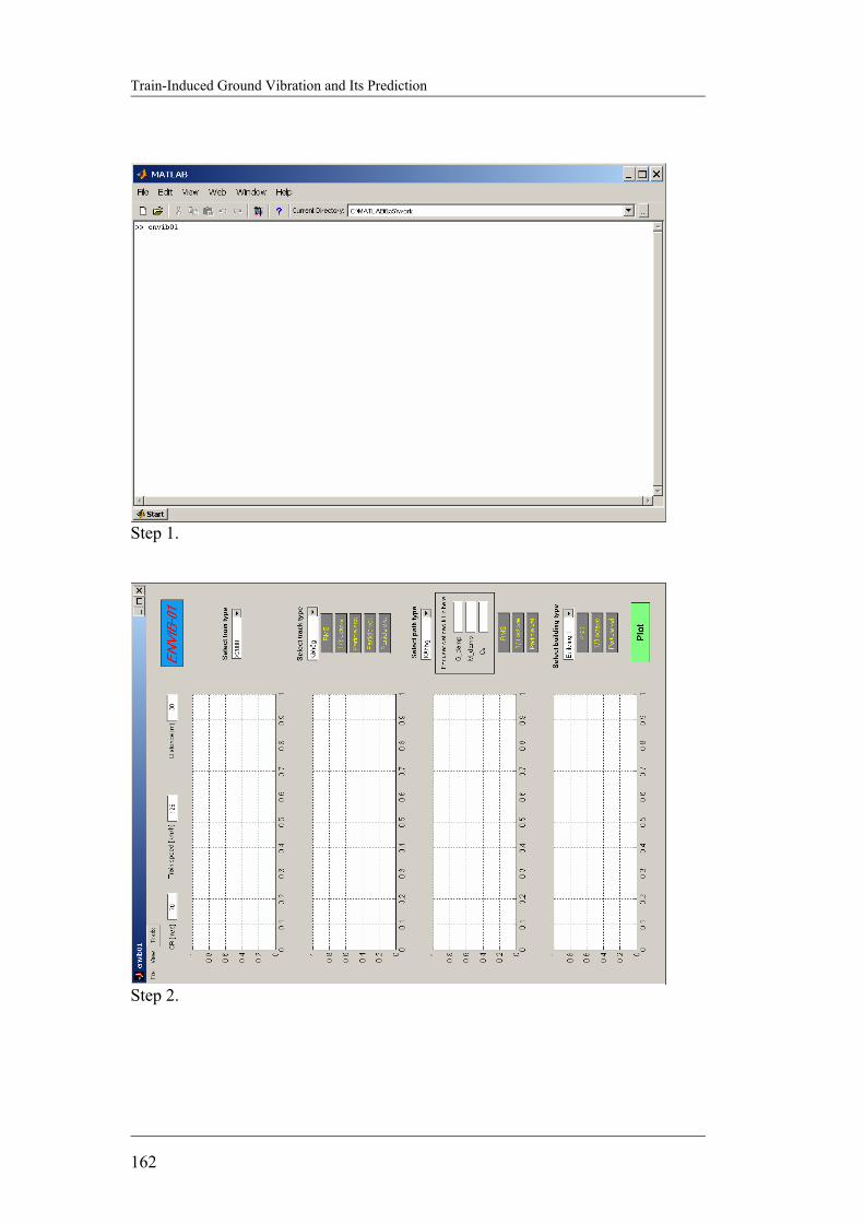
Train-Induced Ground Vibration and Its Prediction
162
Step 1.
Step 2.

Mehdi Bahrekazemi
163
Step 3.
Step 4.
Train-Induced Ground Vibration and Its Prediction
164
Step 5.
Step 6.
Mehdi Bahrekazemi
165
APPENDIX B, TYPICAL RESPONSE CURVES OF THE SENSORS In this appendix the typical response curves for some of the sensors used by Division of Soil and Rock Mechanics at KTH for the measurements discussed in this thesis are presented.
Calibration of a seismometer Mark L-4A
Calibration of a geophone SM-1A 4.5 Hz


Mehdi Bahrekazemi
167
APPENDIX C, SOME DEFINITIONS Some concepts and words used in this thesis may be unfamiliar for part of the audience. Therefore definitions and explanations for some of them are presented here. Were available it has been tried to adopt the definition according to a corresponding ISO or SS-ISO standard. decibel (dB): It is defined as in the Equation C1 where X0 is the reference quantity which is different for particle acceleration and particle velocity and in different countries. While in the US 1E-6 in./sec is used as the reference for particle velocity, 1E-9 m/s, 0.5E-8 m/s, and 1E-8 m/s may be used in Europe as the reference for particle velocity. According to the Swedish standard SS 460 48 61 (1992), 1E-9 m/s and 1E-6 m/s2 are used as reference for particle velocity and particle acceleration respectively.
)log(200X
XdB ⋅= Equation C1
Power Spectral Density, PSD: Mathematically the power spectral density of a sampled stochastic signal is defined as in the following equation and is expressed in physical units of power per hertz (Ljung & Glad, 1991).
2
1
)( )(1lim.)( ∑=
−
∞→=Φ
N
k
ikT
N
Txx ekTx
NT ωω Equation C2
where, T is the sampling period, N is the number of the data points in the signal, and x(kT) is the sampled signal sampled at times kT. Octave: As defined by ISO 2041 (1990) octave is the interval between two frequencies which have a frequency ratio of two. Therefore the interval, in octaves, between any two frequencies is the logarithm to the base 2 of the frequency ratio. One-third octave or third octave: As defined by ISO 2041 (1990) one-third octave or third octave is the interval between two frequencies which have a frequency ratio of 21/3, or 1.2599. Sometimes it is more convenient to use the frequency ratio of 101/10 instead of 21/3. If 101/10 frequency ratio is used, it is called one-tenth decade. One-tenth decades are about 99.9 % of corresponding one-third octaves. This means that there is practically no difference, but for the purpose of this thesis on-third octave is used. Root-mean-square value; r.m.s. value: According to ISO 2041 (1990) the r.m.s. value of a single valued function f(t), over an interval between t1 and t2, is defined as the square root of the average of the squared values of the function over the interval as defined by Equation C3.

Train-Induced Ground Vibration and Its Prediction
168
2/1
2
12
2
1
)(1...
−= ∫
t
t
dttftt
smr Equation C3
if for example r.m.s. value of a discrete time history of particle velocity is needed, the above equation will be modified as given by Equation C4, where vn is the particle velocity sampled with sampling frequency fs.
2/12
...
=∑
N
vsmr n
n
Equation C4
where sfttN )( 12 −= The running r.m.s. value: According to ISO 2631-1 (1997), the running r.m.s. is defined as Equation C5.
( )[ ]2/1
20
0
0
1)(
= ∫−
t
tww dttata
ττ Equation C5
where, aw(t) is the instantaneous frequency weighted acceleration τ is the integration time for running average t is the time (integration variable) t0 is the time of observation (instantaneous time) The one-second-r.m.s. used throughout this thesis is obtained from Equation C5 with τ=1 s .