A new algorithm for spatial impulse response of rectangularplanar transducers

Jiqi Chenga, Jian-yu Lub, Wei Lina, and Yi-Xian Qina,*aDepartment of Biomedical Engineering, Stony Brook University, Stony Brook, NY 11794, USAbDepartment of Bioengineering, the University of Toledo, Toledo, OH 43606, USA

AbstractPrevious solutions for spatial impulse responses of rectangular planar transducers require eitherapproximations or complex geometrical considerations. This paper describes a new, simplified andexact solution using only trigonometric functions and simple set operations. This solution, whichcan be numerically implemented with a straightforward algorithm, is an exact implementation ofthe Rayleigh integral without any far field or paraxial approximation. Additionally, a nonlinearrelationship was also established for spatial impulse responses from two field points which sharethe same projection point on the transducer surface plane. By incorporating this relationship in thealgorithm, the computational efficiency of spatial impulse responses and continuous fields isimproved about 20 folds and 14 folds, respectively. This algorithm has practical applications indesigning 1-D linear/phased arrays, 1.5-D arrays and 2-D arrays, as demonstrated throughnumerical simulations with array transducers. Experiments were also conducted to verify the newsolution and results show that the algorithm is both accurate and efficient. The application of thismethod may include development of ultrasound imaging system for hard and soft tissuenondestructive assessment.

Keywordsarray transducer; field calculation; spatial impulse response; transient field; continuous field;scanning ultrasound

1. IntroductionPulsed excitations are usually employed to generate transient ultrasound fields and to probethe internal structure of objects in ultrasound imaging. Accurate calculation of the transientfield emitted from transducers is very important in transducer design and ultrasound systemoptimization. Harris [1] presented an excellent review on the theories and mathematicalmethods for transient field calculation. For the rigidly baffled planar sources, the mostcommonly employed method is the spatial impulse response approach, originally proposedby Tupholme [2] and later by Stepanishen [3–4]. In the classic treatment, the solution for thelinear lossless wave equation of velocity potential is expressed as the Rayleigh integral.

© 2010 Elsevier B.V. All rights reserved.*Corresponding author. Tel: +1 631 632 1481; Fax: +1 631 632 8577, Yi-Xian.Qin@sunysb.edu (Y. Qin).Publisher's Disclaimer: This is a PDF file of an unedited manuscript that has been accepted for publication. As a service to ourcustomers we are providing this early version of the manuscript. The manuscript will undergo copyediting, typesetting, and review ofthe resulting proof before it is published in its final citable form. Please note that during the production process errors may bediscovered which could affect the content, and all legal disclaimers that apply to the journal pertain.

NIH Public AccessAuthor ManuscriptUltrasonics. Author manuscript; available in PMC 2012 February 1.

Published in final edited form as:Ultrasonics. 2011 February ; 51(2): 229–237. doi:10.1016/j.ultras.2010.08.007.

NIH

-PA Author Manuscript

NIH

-PA Author Manuscript

NIH

-PA Author Manuscript

According to the linear system theory, the integral can be further expressed as the temporalconvolution between the driving velocity and the spatial impulse response between the fieldpoint and the transducer. At each field point, the spatial impulse response is a function oftime. Based on Huygen’s principle, the impulse response can be evaluated usingintersections between the ultrasound source and a spherical wave, which originates from thefield point. Over the years, ultrasound sources of different geometrical shapes, such ascircles [3], rectangles [5–7], triangles [8], polygons [9] and curved strips [10] have beenstudied. In the classic form, the velocity distribution needs to be uniform. To overcome thislimitation, Harris [11] and Tjotta [12] suggested generalized impulse response methods totreat nonuniform velocity distribution on the transducer surface. The impulse responseapproach has also been further developed by Lasota [13] using the line impulse response andby Scarano [14] who expressed impulse response as functions of spatial coordinates insteadof time.

The solution for spatial impulse response is highly dependent on the shape of the sources.The solution for the planar circular source is relatively simple, because only one parameter,such as radius, is needed to describe the source. However, rectangular sources require twoseparate parameters, i.e. width and height, and the solution for the impulse responsebecomes rather complex due to the discontinuities of the intersections. To simplify thesolution, Stepanishen [3] divided the rectangular source into small pieces and applied farfield approximations for each small rectangular source, whose response is a trapezoid. Theimpulse response for the entire source was the summation of the smaller pieces. Lockwoodand Willette [5] were the first to derive the exact solution for rectangular sources. Theydivided the source into four sub-rectangular sections by projecting the field point to thesource surface. The exact expression was given for each subsection, where the projectionpoint is one vertex of the sub-rectangle. The solution for the whole source was finallyexpressed as the superposition of the four subsections. Without using division andsuperposition, the exact solution for a rectangular source can be derived by exhaustivegeometrical considerations of the relative position of the field point to the source. Emeterioand Ullate [7] provided a complete solution after identifying four geometrical areas and atotal of eighteen different conditions. For numerical implementation, Jensen [8–9]developed a new calculation procedure that sorts angles based on geometricalconsiderations. All the described approaches require either approximations or complexgeometrical considerations. Therefore, a simplified and exact solution is needed.

In this work, a new approach was developed to calculate the spatial impulse response forrectangular transducers. With this approach, the exact solution is derived in terms of theelementary operation of sets and trigonometric functions. Compared to previous solutions, ithas several advantages. First, the solution is exact, unlike the solutions provided byStepanishen [3] and Lee and Benkeser [15], where far field approximation is used. Second,the approach does not involve division and superposition like the exact solution provided byLockwood and Willette [5]. Third, the approach is straightforward and easy to implementcompared to the solutions proposed by Emeterio and Ullate [7] and Jensen [8–9] thatinvolve complex geometrical considerations and angle sorting. Additionally, a new,nonlinear relationship is also established for the spatial impulse responses of two differentfield points sharing the same projection point on the transducer surface plane. With thisnonlinear conversion, the new method and algorithm improve the computational efficiencydramatically in numerical implementation.

The solution and the algorithm developed here have broad applications in the transient/continuous field calculations for 1-D linear/phased arrays, 1.5-D arrays and 2-D arrays,which are essential in ultrasound system simulations and optimizations. To demonstratesuch applications, numerical examples of spatial impulse response, transient/continuous

Cheng et al. Page 2

Ultrasonics. Author manuscript; available in PMC 2012 February 1.

NIH

-PA Author Manuscript

NIH

-PA Author Manuscript

NIH

-PA Author Manuscript

fields and transmission/reception system response were provided in the context of a lineararray.

2. TheoryAs shown in Fig. 1(a), a rigidly-baffled rectangular transducer is located on plane z = 0, witha height of h and a width of w. The center of the transducer is at the origin of thecoordinates. According to the Rayleigh integral [1], the solution to the linear lossless scalarwave equation can be expressed as,

(1)

where Φ(x, y, z;t) is the velocity potential; R is the distance between transducer element dsand the field point (x, y, z) ; c is the speed of sound in the media; and u(t) is the uniformvelocity distribution normal to the transducer surface. The term u(t − R / c) can be written inthe integration form,

(2)

Substituting the above equation into Eq. (1) and changing the order of integration yield,

(3)

If a new function is defined as,

(4)

then Eq. (3) can be expressed in a convolution form as,

(5)

where * is the convolution in time domain. The function h(x, y, z;t) is also called the spatialimpulse response of the system at field point (x, y, z).

The spatial impulse response from Eq. (4) can be expressed explicitly as follows,

(6)

Using the relationship R2 = r2 + z2 and according to Ref. [9], the above equation can befurther simplified as,

(7)

Cheng et al. Page 3

Ultrasonics. Author manuscript; available in PMC 2012 February 1.

NIH

-PA Author Manuscript

NIH

-PA Author Manuscript

NIH

-PA Author Manuscript

where Θ1 and Θ2 are determined by the intersection of the transducer and the projectedspherical wave with a radius of R = ct (refer to Fig. 1(a)). The intersection of the spherical

wave with the plane z = 0 is a circle centered at (x, y,0) with a radius of whent > z / c. When the circle intersects the transducer aperture, some intersected arcs are locatedinside the transducer aperture. The angles expanded by these arcs are directly related to thespatial impulse response given by Eq. (7). When more than one arc exists, the spatialimpulse response is the summation of contributions from all arcs, and Eq. (7) is changed tothe following summation:

(8)

where l is the index of the arcs.

To calculate Θ1 and Θ2, we shift the origin of the coordinates to (x, y, 0) and obtain a newcoordinate (x', y', z) as shown in Fig.1 (b). With the new 2-D coordinates at the plane z = 0,the circle can be expressed in polar coordinates as

(9)

If a point on the circle is inside the transducer aperture, the angle Θ must satisfy thefollowing inequalities,

(10)

where x1, x2, y1 and y2 are the coordinates of the four boundaries of the transducer in thenew coordinates given by x1 = −x−w/2, x2 = −x + w/2, y1 = −y−h/2 and y2 = −y + h/2,respectively.

Assuming that Eq. (10)(a) holds when and Eq. (10)(b) also holds when

, we define the following relation,

(11)

where i is the index of the sets that satisfy Eq. (10)(a); j is the index of the sets that satisfyEq.(10)(b); ⋃ is the union of the sets; ⋂ is the intersection of the sets; and each set

corresponds to an arc. When , Eq.(10) is satisfied. With the sets obtainedfrom Eq. (11), the spatial impulse response can be evaluated from Eq. (8).

Calculation of these sets is a matter of trivial algebraic operations involving only elementarytrigonometric functions. Notice that Θ is defined on [0, 2π], but the inverse cosine and

Cheng et al. Page 4

Ultrasonics. Author manuscript; available in PMC 2012 February 1.

NIH

-PA Author Manuscript

NIH

-PA Author Manuscript

NIH

-PA Author Manuscript

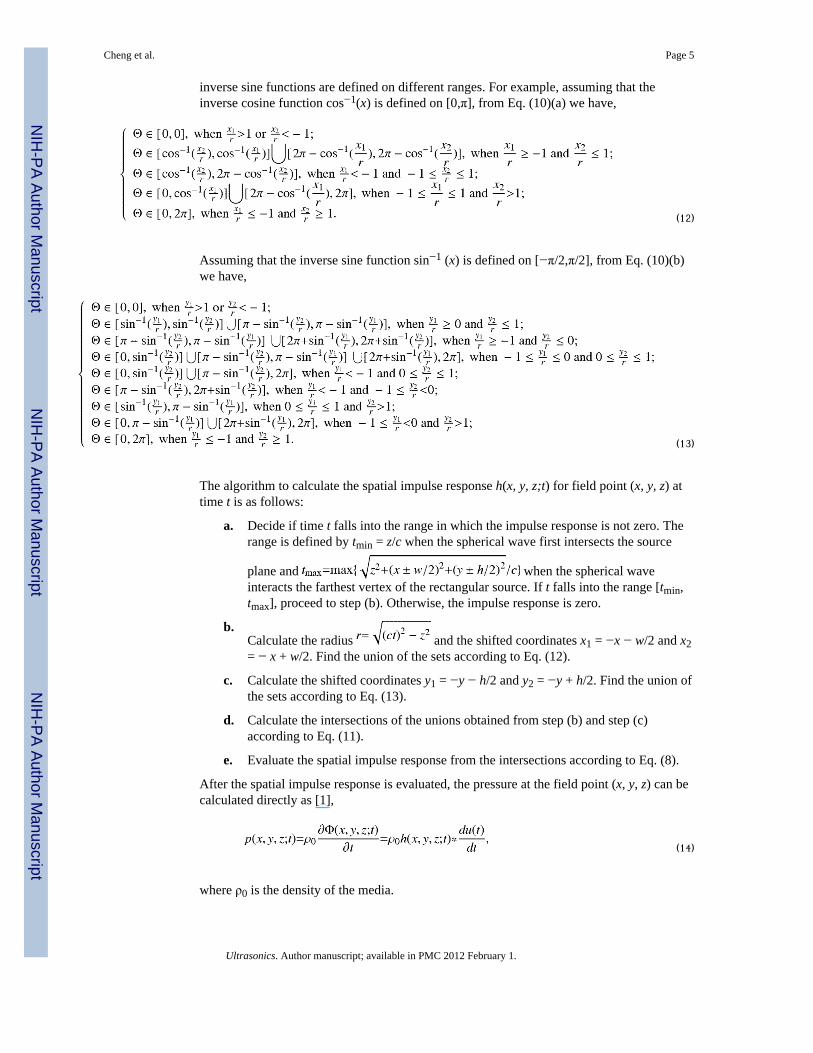
inverse sine functions are defined on different ranges. For example, assuming that theinverse cosine function cos−1(x) is defined on [0,π], from Eq. (10)(a) we have,

(12)

Assuming that the inverse sine function sin−1 (x) is defined on [−π/2,π/2], from Eq. (10)(b)we have,

(13)

The algorithm to calculate the spatial impulse response h(x, y, z;t) for field point (x, y, z) attime t is as follows:

a. Decide if time t falls into the range in which the impulse response is not zero. Therange is defined by tmin = z/c when the spherical wave first intersects the source

plane and when the spherical waveinteracts the farthest vertex of the rectangular source. If t falls into the range [tmin,tmax], proceed to step (b). Otherwise, the impulse response is zero.

b.Calculate the radius and the shifted coordinates x1 = −x − w/2 and x2= − x + w/2. Find the union of the sets according to Eq. (12).

c. Calculate the shifted coordinates y1 = −y − h/2 and y2 = −y + h/2. Find the union ofthe sets according to Eq. (13).

d. Calculate the intersections of the unions obtained from step (b) and step (c)according to Eq. (11).

e. Evaluate the spatial impulse response from the intersections according to Eq. (8).

After the spatial impulse response is evaluated, the pressure at the field point (x, y, z) can becalculated directly as [1],

(14)

where ρ0 is the density of the media.

Cheng et al. Page 5

Ultrasonics. Author manuscript; available in PMC 2012 February 1.

NIH

-PA Author Manuscript

NIH

-PA Author Manuscript

NIH

-PA Author Manuscript

From the algorithm and Eqs (8)–(13), it is obvious that the spatial impulse response h(x, y,z;t) depends on the shifted coordinates x1, x2, y1, y2 and the radius r. If the two coordinates, xand y, of the field points are fixed, spatial impulse response would only depend on radius r.

For two field points (x, y, z0) and (x, y, z1), if equals to , thespatial impulse responses at the two field points are equal for these specific moments anddistances, i.e. h(x, y, z0;t0) = h(x, y, z1;t1). From

(15)

we have

(16)

where t0 ≥ z0 / c and t1 ≥ z1 / c. Thus we have the following relationship,

(17)

If z0 is set to zero, we get the following after changing the variables:

(18)

Eq. (18) has an important implication for numerical calculation of the spatial impulseresponse. It means that the spatial impulse response at one field point can be directly relatedto the response at another point, which is the projection at the transducer surface plane. Weonly need to calculate the spatial impulse response h(x, y,0;t) at (x, y,0) once and save it as alookup table. The spatial impulse response h(x, y, z;t) at field point (x, y, z) can be evaluated

as with one simple nonlinear conversion of time t. For applicationswhere time is evenly sampled, we are attempting to evaluate h(x, y, z;nΔT2) from h(x, y,0;mΔT1), where ΔT1 and ΔT2 are the sampling intervals for h(x, y,0;t) and h(x, y, z;t)respectively and m and n are natural integers. After nonlinear conversion, we have

(19)

The converted time may not exactly fall on the sampled time point. Linearinterpolation is needed, and we get

(20)

Cheng et al. Page 6

Ultrasonics. Author manuscript; available in PMC 2012 February 1.

NIH

-PA Author Manuscript

NIH

-PA Author Manuscript

NIH

-PA Author Manuscript

To reduce the numerical error introduced by the interpolation, a smaller sampling intervalΔT1 can be used to generate the lookup table, which needs to be calculated only once.

3. ResultsIn this section, applications of the algorithm are demonstrated through numericalsimulations and experimental validations. The spatial impulse responses, transient fields,continuous fields and echo signals were calculated for a linear array transducer. Theapplications for 1.5-D or 2-D arrays can be easily formulated following the same procedure.Experiments were carried out to verify the simulation results of the echo signals. Theinfluences of sampling rate, computational efficiency and accuracy were also addressed.

3.1 Simulation conditionsFor numerical simulations, we assumed a linear array transducer with 128 elements. It has apitch of 0.15 mm, physical dimensions of 19.2 mm × 14 mm, and a central frequency of 2.5MHz. It models a commercial V2 array transducer from Acuson that was used in theexperimental setup. There is no focusing in elevation for numerical simulations while thephysical transducer does have one with a focal distance of 68 mm.

For simplicity, the transfer function of the transducer in the simulation was assumed to be aBlackman window for both transmission and reception,

(21)

The two-way fractional bandwidth of this function is 64% of the central frequency at −6 dBand the bandwidth of the physical transducer V2 is about 50% to 60%.

The driving signal for each element in the transient field and echo simulation was a one-cycle sine wave at 2.5 MHz without any time delay, which was also used in the experiments.For continuous field simulation, the driving signal at each element was a continuous sinewave at 2.5 MHz with an initial phase of zero. The weighting level for every element in bothsimulation and experiment was set to be one and the unit of measurement for the coordinatesdefined in the following subsections is mm.

The algorithm developed in this study and the classic method developed by Lockwood andWillette [5], which was used as a standard for comparison, were both implemented using Clanguage. The algorithms were tested under the Linux operating system on a PC equippedwith dual processors running at 2.8 GHz and a total internal memory of 2 Gbytes.

For numerical error calculation, two paired signals were first normalized separately. Then,the error signal was defined as the absolute difference between the two normalized signals.The maximum error was detected by scanning the error signal from beginning to the end.When two images with multiple paired signals were compared, the overall maximum erroracross all pairs was obtained by finding the maximum of the maximum errors of each pair.The maximum error is expressed as a percentage.

3.2 Impulse Response for array transducerFor a linear array consisting of N flat transducer elements, the impulse response of thewhole transducer can be treated as the summation of the individual impulse responses fromeach element if the same driving signal is applied all elements.

Cheng et al. Page 7

Ultrasonics. Author manuscript; available in PMC 2012 February 1.

NIH

-PA Author Manuscript

NIH

-PA Author Manuscript

NIH

-PA Author Manuscript

As shown in Fig. 2, the spatial impulse response of the whole transducer for a linear arraycan be expressed as

(22)

where h(x, y, z;t) is the spatial impulse response of the whole transducer; i = 0,1, … ,N − 1,is the index of the elements of the array; ai is the weighting level at element i; hi(x, y, z;t) isthe spatial impulse response between the element i and the field point (x, y, z), which can becalculated according to Eq. (8). However, Eq. (8) only applies when the center of thetransducer is located at the origin. Therefore, the origin of the coordinates needs to beshifted to the center of each element and the coordinates of the field point need to bechanged accordingly.

The spatial impulse responses of the linear transducer defined in section 3.1 were calculated.The field points were on two typical lines defined by (0,0, z) and (20,0, z) (refer to Fig. 2 forthe definition of the coordinates). One of the lines (0,0, z) has a projection point (0,0,0) thatlies inside the transducer aperture, while the projection point (20,0,0) from the other line isoutside the transducer aperture.

Fig. 3 shows selected plots of normalized spatial impulse responses at different distancesalong the line defined by (0,0, z). For clarity, the responses at different distances werevertically shifted in a progressive manner. In reality, all these responses share the same baseline of zero. The plots in dashed lines were calculated according to the new algorithm withthe nonlinear conversion defined in Eq. (18). The plots in solid lines were calculated directlyaccording to the classic method by Lockwood and Willette [5]. Following the same format,Fig. 4 shows plots of spatial impulse responses along another line defined by (20,0, z).

The spatial impulse responses along these two lines have very distinct features. If a line hasa projection point inside the transducer aperture, the spatial impulse responses along the linejump suddenly from zero to their maxima. On the other hand, if the line has a projectionpoint lying outside of the transducer aperture, the spatial impulse responses graduallyincrease to their maxima. However, the spatial impulse responses for field points along thesame line share the same basic characteristics. When a point is further away from thetransducer, the main features of the impulse response are condensed in time, and theduration is reduced. This phenomenon is predicted by Eq. (18) and is the base for nonlinearconversion. These characteristics of the impulse response have some influence on numericalimplementations. When field points further away from the transducer surface are considered,a higher temporal sampling rate is required to meet the sampling requirement and avoidaliases.

For Fig. 3, the spatial impulse responses of 800 field points along the line (0,0, z) werecalculated with a sampling distance of 0.15 mm. It took 15.64 seconds for the new algorithmand 318.42 seconds for the classic method. There is a 20-fold increase in calculation speed.For the field points along line (20,0, z), similar speed improvement was observed. Fromthese selected plots in both Fig. 3 and Fig. 4, it is difficult to tell the difference in the resultscalculated from the different algorithms. However, the numerical implementation of thenonlinear conversion introduced some error to the spatial impulse responses when comparedto the responses calculated directly with the classic method, which is exact at specificsampling frequency. With a temporal sampling frequency of 100 MHz, the maximum errorsacross all the field points were 1.55% and 2.40% for the lines (0,0, z) and (20,0, z)respectively.

Cheng et al. Page 8

Ultrasonics. Author manuscript; available in PMC 2012 February 1.

NIH

-PA Author Manuscript

NIH

-PA Author Manuscript

NIH

-PA Author Manuscript

3.3 Transient Field calculation for array transducerTo calculate the transient field at point (x, y, z) for a linear array transducer, one can add thepressure from each element (as defined in Eq. (14)) together as follows,

(23)

where ui (t) is the velocity profile for element i, and all the other parameters have the samedefinitions as those in Eq. (22). Here, the velocity profile of each element does not have tobe the same. For example, to generate a focused pulse, a different time delay is needed foreach element, and the velocity profile ui (t) has to be different for every element.

Fig. 5 shows the transient fields for four selected points at (0,0,60), (6,0,60), (0,0,120) and(6,0,120). A pulsed plane wave was simulated, and the transmit transfer function defined byEq. (21) was also included and acted as a band pass filter for the excitation signal. The timeduration of these transient fields was truncated to a window of 5 µs with the starting momentshifted to show details of the wave.

The temporal sampling frequency has a major influence on the numerical accuracy of thetransient fields calculated using all spatial impulse response approaches. The studyconducted by Crombie [16] showed that the maximum error is about 5% at a sampling rateof 250 MHz for exact solutions. The errors were calculated by comparing the fields to thosecalculated with a sampling rate of 4 GHz. For the linear array defined here, the maximumerrors of the transient fields are calculated for 128 field points with a spatial samplingdistance of 0.15 mm on a line defined by (x,0,120). At sampling frequencies of 40 MHz, 160MHz, 320 MHz and 640 MHz, the maximum errors are 13.7%, 2.67%, 1.14% and 0.69%,respectively. These errors were calculated using the transient field at 5120 MHz as thestandard for comparison, since an even higher sampling rate would not significantly improveaccuracy. The base frequency of 40 MHz was chosen because it was the sampling frequencyused in the experiment. Considering the different transducer configurations involved, theresults agree with those in literature. For the field point (x, y, z) with a projection point lyinginside the transducer aperture, the spatial impulse response jumps suddenly from zero tomaximum at the moment t = z / c as shown in Fig. 3. Theoretically, the sampling frequencyhas to be infinite to capture the sudden jump at the precise moment. When finite samplingfrequency is used, the starting moment of the spatial impulse response always has anuncertainty of ΔT, which is the temporal sampling interval. If the transient field shape, notthe starting moment, is the major concern, the uncertainty can be partially corrected byshifting the starting moment within ΔT. With the correction, the maximum errors at 40MHz, 160 MHz, 320 MHz and 640 MHz drop significantly to 3.90%, 0.98%, 0.43%, and0.30% respectively, which implies that the sampling rate does not have to be extremely highto have acceptable accuracy in terms of the shape of the transient field.

3.4 Continuous Field calculation for array transducerThe continuous field is a special case of transient fields, where the excitation is a continuousharmonic wave instead of a pulse. Referring to Eq. (14), if u(t) = ej(ω 0t+ϕ), we have

(24)

where ω0 and ϕ are the angular frequency and initial phase of the driving signal respectively.Eq. (24) can be explicitly rewritten as

Cheng et al. Page 9

Ultrasonics. Author manuscript; available in PMC 2012 February 1.

NIH

-PA Author Manuscript

NIH

-PA Author Manuscript

NIH

-PA Author Manuscript

(25)

Defining the time domain Fourier transform of h(x, y, z;t) as

(26)

Eq. (25) can be simplified as follows,

(27)

For array transducer, if every element is driven at the same frequency ω0; from Eq. (23) andEq. (27), we obtain

(28)

where Hi (x, y, z; ω0) is the Fourier transform of hi(x, y, z; t) evaluated at frequency ω0, andϕi is the initial phase of the driving signal at element i. When the initial phases of eachelement are the same, a continuous plane wave can be obtained. For a continuous focusedwave, the initial phases at different elements need to be different.

The continuous plane-wave fields at central frequency of 2.5 MHz for the array transducerwere calculated and displayed in Fig. 6. The amplitude of the fields was normalized and log-compressed to −40 dB. The field points are located on the plane defined by (x,0, z) withdimensions of 38.4 mm by 120 mm. The spatial sampling distance is 0.15 mm in eachdirection. The field in panel (a) is calculated using the method developed in this study withnonlinear conversion, while the one in panel (b) is evaluated directly using the classicmethod. It took 52.5 minutes and 746.2 minutes to calculate panel (a) and panel (b)respectively at a temporal sampling frequency of 100 MHz. In terms of the computationalefficiency, an improvement of 14 folds is achieved with the new method. The nonlinearconversion only introduces a negligible maximum error of 0.49% across all field points.

For continuous field calculation, the spatial impulse response approach has a unique feature.As seen in Eqs. (24)–(28), one has to calculate the time-domain spatial impulse response,which is the most time-consuming part, before calculating the continuous field at onespecific frequency. The next step is to obtain the Fourier transform of these responses. WithFast Fourier Transform, the continuous fields at all frequencies, which are smaller than halfof the sampling frequency, are calculated at the same time. This allows the continuous fieldsat all frequencies to be evaluated without further calculations. In addition, this approach cancalculate the continuous field starting right from the transducer surface unlike the classicRayleigh-Sommerfeld method [17] which is unable to do so because it needs numericaldouble integration. When the field point gets too close to the source, the phases change toorapidly for the integration to converge. To overcome the limitation of the Rayleigh-Sommerfeld method, the distribute point source method (DPSM) [18–20] was recentlyproposed. This method uses distributed point sources located slightly behind the transducersurface to model the transducer. In this way, the continuous field that starts right from thetransducer surface can be calculated by summing the contribution from all point sources,whose strengths are determined by the boundary condition on the transducer surface.

Cheng et al. Page 10

Ultrasonics. Author manuscript; available in PMC 2012 February 1.

NIH

-PA Author Manuscript

NIH

-PA Author Manuscript

NIH

-PA Author Manuscript

Detailed comparisons between DPSM and our approach are beyond the scope of this paper.Therefore, only a brief comparison will be made here. When implemented under the sameconditions as described in Section 3.1, DSPM took 8.1 minutes and 32.4 minutes tocalculate the same field when 128×93 and 256×186 point sources of uniform strength wereused, respectively. These fields are displayed in Fig. 7. The maximum errors of these twofields compared to the field calculated with the classic method (as displayed in Fig. 6(b)),are 20.48% and 11.62%, respectively. The maximum error decreases when the density of thepoint sources increases, however these errors are all significantly higher than the error fromour method (as displayed in Fig. 6(a)), which is 0.49%. It is obvious that the density of thedistributed point sources for DPSM has to be increased to improve accuracy, which in turn,would increase calculation time dramatically. On the other hand, the calculation time of ourmethod was reduced to only 5.2 minutes when one single large-aperture transducer, insteadof the 128-element array transducer, was assumed in implementation. Take note that theerrors for DPSM are noticeably higher than those described in Ref. [20]. This could possiblybe due to the fact that off-axis field points were included in this work and differentcomparison criteria were used.

3.5 Echo simulation and experiment for array transducerBased on the linear system theory [16,21], the pulse-echo response of a linear arraytransducer can be easily modeled. When one point at (x, y, z) (refer to Fig. 2) is insonifed byultrasound, it scatters the ultrasound with a coefficient f (x, y, z). Then the scatteredultrasound received by an element of the array transducer is given by [21],

(29)

If the electro-mechanical transfer function of the array is B(t), then the electrically receivedecho signal from element i can be expressed as,

(30)

When weak scattering approximation or First Born approximation [22] is assumed, oneobtains the echo signals from multiple scattering points as the summation of thecontributions from each point as defined in Eq. (30).

Echo signals were simulated and experimentally collected for four separate points withcoordinates of (0,0,30), (0,0,50), (0,0,70) and (0,0,90) respectively. The experiment wasconducted in degassed water at room temperature and a small glass ball with a diameter of0.5 mm served as a point scatterer. The scatterer was placed at the center of the transducerand vertically descended to an appropriate depth using a stepping motor. The depth was alsoindependently verified by the time of flight of the echoes. The echo data was digitized with aresolution of 12 bits and a sampling frequency of 40 MHz by a self-built ultrasound imagingsystem [23] that has 128 independent transmit/receive channels.

Fig. 8 shows the echo signals with time duration of 5 µs. The echo signals detected by all128 elements were converted to grey scale and arranged in parallel to form a 2D image. Thehorizontal dimension for these images is time, while the vertical dimension is the index ofeach element, starting from 0 to 127. Fig. 9 shows the line plots of the normalized echoes at

Cheng et al. Page 11

Ultrasonics. Author manuscript; available in PMC 2012 February 1.

NIH

-PA Author Manuscript

NIH

-PA Author Manuscript

NIH

-PA Author Manuscript

element 64. The simulated echo signals are displayed in solid lines and the experimentalones in dashed lines.

From these two figures, one can observe that the simulation agrees with the experimentfairly well. The main features of the echoes from the simulation were very similar to thosefrom the experiment. However, some differences do exist. For example, the echoes in theexperiment last longer than those in the simulation. There are several possible causes forsuch differences. First, the transfer function used in the simulation was the well-definedBlackman window whose two-way bandwidth is slightly higher than that of the physical V2transducer, resulting in a shorter pulse. Second, an ideal point scatterer was assumed in thesimulation, while a glass ball with a diameter close to the central wavelength of thetransducer was used in the experiment. Third, there is a physical focus at 68mm in elevationfor the V2 transducer while no focusing in elevation was assumed in simulation.

4. ConclusionSpatial impulse response method is very important for transient, continuous fieldcalculations and transducer designs. The previous solutions of the spatial impulse responsefor rectangular planar transducers required divisions and superposition, complicatedgeometrical considerations or far field approximations. In this study, we developed a simpleand exact solution involving only elementary trigonometric functions and simple setoperations. A nonlinear relationship was also established for the spatial impulse responsesfrom two field points sharing the same projection point in the transducer surface plane.Coupled with this nonlinear conversion, the new method achieved a 20-fold and 14-foldincrease in computational efficiency for spatial impulse response calculation and continuousfield calculation respectively. This method may have potential to improve the design ofultrasound imaging system for hard and soft tissue nondestructive assessment.

AcknowledgmentsThis work is kindly supported by the National Space Biomedical Research Institute through NASA CooperativeAgreement NCC 9-58, the NIH (AR52379), and US Army Medical Research. The authors are also grateful to Mr.Alain Rivolle, Professor Dominique Placko and Professor Tribikram Kundu for their help on the DPSM method.

References1. Harris GR. Review of transient field theory for a baffled planar piston. J. Acoust. Soc. Am

1981;70:10–20.2. Tupholme GE. Generation of acoustic pulses by baffled plane pistons. Mathematika 1969;16:209–

224.3. Stepanishen PR. Transient Radiation from Pistons in an Infinite Planar Baffle. J. Acoust. Soc. Am

1971;49:1629–1638.4. Stepanishen PR. The time-dependent force and radiation impedance on a piston in a rigid infinite

planar baffle. J. Acoust. Soc. Am 1971;49:841–849.5. Lockwood JC, Willette JG. High-speed Method for Computing the Exact Solution for the Pressure

Variations in the Nearfield of a Baffled Piston. J. Acoust. Soc. Am 1973;53:735–741.6. Ullate LG, Emeterio JLS. a new algorithm to calcualte the transient near-field of ultrasonic phased

arrays. IEEE Trans. Ultrason., Ferroelect.,Freq. Contr 1992;39:745–753.7. Emeterio JLS, Ullate LG. Diffraction Impulse Response of Rectangular Transducers. J. Acoust. Soc.

Am 1992;92:651–662.8. Jensen JA. Ultrasound Fields From Triangular Apertures. J. Acoust. Soc. Am 1996;100:2049–2056.9. Jensen JA. A new calculation procedure for spatial impulse responses in ultrasound. J. Acoust. Soc.

Am 1999;105:3266–3274.

Cheng et al. Page 12

Ultrasonics. Author manuscript; available in PMC 2012 February 1.

NIH

-PA Author Manuscript

NIH

-PA Author Manuscript

NIH

-PA Author Manuscript

10. Faure P, Cathignol D, Chapelon JY, Newhouse VL. On the Pressure Field of a Transducer in theForm of a Curved Strip. J. Acoust. Soc. Am 1994;95:628–637.

11. Harris GR. Transient Field of a Baffled Planar Piston Having an Arbitrary Vibration AmplitudeDistribution. J. Acoust. Soc. Am 1981;70:186–204.

12. Tjotta JN, Tjotta S. Nearfield and Farfield of Pulsed Acoustic Radiators. J. Acoust. Soc. Am1982;71:824–834.

13. Lasota H, Salamon R, Delannoy B. Acoustic Diffraction Analysis by the Impulse ResponseMethod a Line Impulse Response Approach. J. Acoust. Soc. Am 1984;76:280–290.

14. Scarano G, Denisenko N, Matteucci M, Pappalardo M. A New Approach to the Derivation of theImpulse Response of a Rectangular Piston. J. Acoust. Soc. Am 1978;78:1109–1113.

15. Lee C, Benkeser PJ. A Computationally Efficient Method for the Calculation of the Transient Fieldof Acoustic Radiators. J. Acoust. Soc. Am 1994;96:545–551.

16. Crombie P, Bascom PAJ, Cobbold RSC. Calculating the Pulsed Response of Linear Arrays:Accuracy Versus Computational Efficiency. IEEE Trans. Ultrason., Ferroelect.,Freq. Contr1997;44:997–1009.

17. Goodman, JW. Introduction to Fourier Optics. 2nd ed.. New York: McGraw-Hill; 1996.18. Kundu, T. Ultrasonic nondestructive evaluation : engineering and biological material

characterization. Boca Raton, Fla: CRC Press; 2004.19. Placko, D.; Kundu, T. DPSM for modeling engineering problems. Hoboken, N.J: Wiley-

Interscience; 2007.20. Kundu T, Placko D, Kabiri Rahani E, Yanagita T, Minh Dao C. Ultrasonic Field Modelling: A

Comparision between Analytical, Semi-Analystical and Numerical Techniques. IEEE Trans.Ultrason., Ferroelect.,Freq. Contr. (In Press).

21. Jensen JA. Linear description of ultrasound imaging systems, notes for the international summerschool on advanced ultrasound imaging. DTU, Technical Report. 1999

22. Kak, AC.; Slaney, M. Principle of computerized tomographic imaging. New York: IEEE Press;1987.

23. Lu JY, Cheng J, Wang J. High frame rate imaging system for limited diffraction array beamimaging with square-wave aperture weightings. IEEE Trans. Ultrason., Ferroelect.,Freq. Contr2006;53:1796–1812.

Cheng et al. Page 13

Ultrasonics. Author manuscript; available in PMC 2012 February 1.

NIH

-PA Author Manuscript

NIH

-PA Author Manuscript

NIH

-PA Author Manuscript

Fig. 1.Geometry of the transducer and the filed point. (a) Spherical intersection in original 3-Drectangular coordinates. (b) Spherical intersection in the shifted 2-D coordinates.

Cheng et al. Page 14

Ultrasonics. Author manuscript; available in PMC 2012 February 1.

NIH

-PA Author Manuscript

NIH

-PA Author Manuscript

NIH

-PA Author Manuscript

Fig. 2.The geometry of the array transducer and field point.

Cheng et al. Page 15

Ultrasonics. Author manuscript; available in PMC 2012 February 1.

NIH

-PA Author Manuscript

NIH

-PA Author Manuscript

NIH

-PA Author Manuscript

Fig. 3.The plots of the spatial impulse response along line (0,0,z) with the unit being mm.

Cheng et al. Page 16

Ultrasonics. Author manuscript; available in PMC 2012 February 1.

NIH

-PA Author Manuscript

NIH

-PA Author Manuscript

NIH

-PA Author Manuscript

Fig. 4.The plots of the spatial impulse response along line (20,0,z) with the unit being mm.

Cheng et al. Page 17

Ultrasonics. Author manuscript; available in PMC 2012 February 1.

NIH

-PA Author Manuscript

NIH

-PA Author Manuscript

NIH

-PA Author Manuscript

Fig. 5.The plots of transient fields at four points: (a) (0,0,60), (b) (6,0,60), (c) (0,0,120), (d)(6,0,120) with the unit being mm.

Cheng et al. Page 18

Ultrasonics. Author manuscript; available in PMC 2012 February 1.

NIH

-PA Author Manuscript

NIH

-PA Author Manuscript

NIH

-PA Author Manuscript

Fig. 6.Continuous plane wave fields for the array transducer at 2.5 MHz: (a) New method, (b)Classic method.

Cheng et al. Page 19

Ultrasonics. Author manuscript; available in PMC 2012 February 1.

NIH

-PA Author Manuscript

NIH

-PA Author Manuscript

NIH

-PA Author Manuscript

Fig. 7.Continuous plane wave fields for the array transducer at 2.5 MHz: (a) DPSM with 128×93point sources, (b) DPSM with 256×186 point sources.

Cheng et al. Page 20

Ultrasonics. Author manuscript; available in PMC 2012 February 1.

NIH

-PA Author Manuscript

NIH

-PA Author Manuscript

NIH

-PA Author Manuscript

Fig. 8.Simulated and experimental echo signals: (a)–(d) are simulated results for 4 points at thecenter of the transducer with a distance of 30 mm, 50 mm, 70 mm and 90 mm away from thetransducer surface respectively. (e)–(i) are experimental results in water for the same pointsas in (a)–(d). The vertical dimension is the index of elements of the transducer, and thehorizontal dimension is time.

Cheng et al. Page 21

Ultrasonics. Author manuscript; available in PMC 2012 February 1.

NIH

-PA Author Manuscript

NIH

-PA Author Manuscript

NIH

-PA Author Manuscript

Fig. 9.The plots of echo signals at element 64 as in Fig. 8: (a) z=30 mm, (b) z=50 mm, (c) z=70mm, (d) z=90 mm.

Cheng et al. Page 22

Ultrasonics. Author manuscript; available in PMC 2012 February 1.

NIH

-PA Author Manuscript

NIH

-PA Author Manuscript

NIH

-PA Author Manuscript