UCRL-TR-236581

A Finite-Difference Numerical Method forOnsager's Pancake Approximation forFluid Flow in a Gas Centrifuge

M. de Stadler, K. Chand

November 15, 2007

Disclaimer

This document was prepared as an account of work sponsored by an agency of the United States government. Neither the United States government nor Lawrence Livermore National Security, LLC, nor any of their employees makes any warranty, expressed or implied, or assumes any legal liability or responsibility for the accuracy, completeness, or usefulness of any information, apparatus, product, or process disclosed, or represents that its use would not infringe privately owned rights. Reference herein to any specific commercial product, process, or service by trade name, trademark, manufacturer, or otherwise does not necessarily constitute or imply its endorsement, recommendation, or favoring by the United States government or Lawrence Livermore National Security, LLC. The views and opinions of authors expressed herein do not necessarily state or reflect those of the United States government or Lawrence Livermore National Security, LLC, and shall not be used for advertising or product endorsement purposes.

This work performed under the auspices of the U.S. Department of Energy by Lawrence Livermore National Laboratory under Contract DE-AC52-07NA27344.

A Finite-Difference Numerical Method for Onsager’s Pancake

Approximation for Fluid Flow in a Gas Centrifuge

Matthew de Stadler

Lawrence Livermore National Laboratory

Kyle Chand∗

Lawrence Livermore National Laboratory

November 12, 2007

Contents

abstract . . . . . . . . . . . . . . . . . . . . . . . . . . . . . . . . . . . . . . . . . . . . . . . . . . 2

1 Introduction 2

2 Equations of Motion in Axisymmetric Coordinates 2

2.1 Wheel Flow Equilibrium Solution . . . . . . . . . . . . . . . . . . . . . . . . . . . . . . . . . 3

3 Linearizing the Equations of Motion 3

3.1 Linearizing Transformations . . . . . . . . . . . . . . . . . . . . . . . . . . . . . . . . . . . . . 33.2 Linearized Equations of Motion . . . . . . . . . . . . . . . . . . . . . . . . . . . . . . . . . . . 33.3 Deriving Onsager’s Master Equation . . . . . . . . . . . . . . . . . . . . . . . . . . . . . . . . 43.4 Non-Dimensional Form of Onsager’s Master Equation . . . . . . . . . . . . . . . . . . . . . . 6

4 Solving Onsager’s Master Equation 7

4.1 Coupled System of Partial Differential Equations . . . . . . . . . . . . . . . . . . . . . . . . . 74.2 Boundary Conditions: Total Reflux Case . . . . . . . . . . . . . . . . . . . . . . . . . . . . . . 84.3 Problem Parameters . . . . . . . . . . . . . . . . . . . . . . . . . . . . . . . . . . . . . . . . . 84.4 Choosing A Suitable Grid . . . . . . . . . . . . . . . . . . . . . . . . . . . . . . . . . . . . . . 8

5 Results 9

5.1 Verification . . . . . . . . . . . . . . . . . . . . . . . . . . . . . . . . . . . . . . . . . . . . . . 115.2 Validation . . . . . . . . . . . . . . . . . . . . . . . . . . . . . . . . . . . . . . . . . . . . . . . 135.3 Known Errors . . . . . . . . . . . . . . . . . . . . . . . . . . . . . . . . . . . . . . . . . . . . . 13

6 Conclusion 13

7 Future Work 16

A Pseudocode for Simulation 16

∗For correspondence on this paper contact Kyle Chand at chand1@llnl.gov

1

Abstract

Onsager’s pancake approximation is used to construct a simulation to model fluid flow in a gas

centrifuge. The governing 6th order partial differential equation is broken down into an equivalent

coupled system of three equations and then solved numerically. In addition to a discussion on the

baseline solution, known problems and future work possibilities are presented.

1 Introduction

Gas centrifuges exhibit very complex flows. Within the centrifuge there is a rarefied region, a transitionregion, and a region with an extreme density gradient. The flow moves at hypersonic speeds and shockwaves are present. However, the flow is subsonic in the axisymmetric plane.

The analysis may be simplified by treating the flow as a perturbation of wheel flow. Wheel flow impliesthat the fluid is moving as a solid body. With the very large pressure gradient, the majority of the fluidis located very close to the rotor wall and moves at an azimuthal velocity proportional to its distance fromthe rotor wall; there is no slipping in the azimuthal plane. The fluid can be modeled as incompressible andsubsonic in the axisymmetric plane. By treating the centrifuge as long, end effects can be appropriatelymodeled without performing a detailed boundary layer analysis.

2 Equations of Motion in Axisymmetric Coordinates

The equations of motion for a steady-state axisymmetric fluid in cylindrical coordinates are as follows. It isassumed that temperature differences in the fluid are minimal which results in a constant viscosity, constantspecific heat, and constant thermal conductivity of the gas. These equations are the starting point for theanalysis of fluid flow in a gas centrifuge.

Mass continuity:

1

r

∂

∂r(ρrVr) +

∂

∂z(ρVz) = 0 (1)

Axial momentum:

ρ

(

Vr∂Vz

∂r+Vz

∂Vz

∂z

)

= −∂p

∂z+µ

1

r

∂

∂r

(

r∂Vz

∂r

)

+∂2Vz

∂z2

+ ρg (2)

Radial momentum:

ρ

(

Vr∂Vr

∂r−V 2

θ

r+Vz

∂Vr

∂z

)

= −∂p

∂r+µ

∂

∂r

[

1

r

∂

∂r(rVr)

]

+∂2Vr

∂z2

(3)

Azimuthal momentum:

ρ

(

Vr∂Vθ

∂r+VrVθ

r+Vz

∂Vθ

∂z

)

= µ

∂

∂r

[

1

r

∂

∂r(rVθ)

]

+∂2Vθ

∂z2

(4)

Energy equation:

ρCv

(

Vr∂T

∂r+Vz

∂T

∂z

)

+ T

(

∂p

∂T

)

ρ

[

1

r

∂

∂r(rVr) +

∂Vz

∂z

]

= κ

[

1

r

∂

∂r

(

r∂T

∂r

)

+∂2T

∂z2

]

(5)

where r is the radius, ρ the density, p the pressure, T the temperature, µ the viscosity, g gravity, Cv thespecific heat at constant volume of the gas, and κ the thermal conductivity of the gas. Vr, Vz, and Vθ arethe velocity components in the radial, axial, and azimuthal directions, respectively.is this section indented... how do I fix this?

2

Equation of state for an ideal gas:

p = ρRT (6)

where R is the general gas constant, M the molecular weight and R is defined as follows

R =R

M

2.1 Wheel Flow Equilibrium Solution

It is helpful to construct a solution for the case when the fluid in the gas centrifuge is in equilibrium. Thisoccurs in the ideal case where flow perturbations due to thermal or mechanical effects do not exist.

Vr = 0

Vθ = Ωr

Vz = 0

T = T0

(

∂p

∂z

)

0

= ρ0g ≈ 0 (7)

(

∂p

∂r

)

0

= ρ0Ω2r =

p0

RT0Ω2r (8)

where Ω is the rotation rate of the cylinder wall. Integration of Equation 8 results in

p0(r) = p(0)exp[(MΩ2/2RT0)r2] (9)

ρ0(r) = ρ(0)exp[(MΩ2/2RT0)r2] (10)

3 Linearizing the Equations of Motion

3.1 Linearizing Transformations

Each of the problem relevant primitive variables are written as a combination of an equilibrium value and aperturbation value.

Vz = 0 + u ρ = ρ0 + ρ

Vr = 0 + v p = p0 + p

Vθ = Ωr + w T = T0 + T

where u, v, and w represent the perturbation velocities in the axial, radial, and azimuthal direction. Pertur-bations of the gas due to internal circulation are given by p, ρ, and T .

3.2 Linearized Equations of Motion

After applying the linearizing transformations and neglecting the products of perturbation values, also ne-glecting the effect of gravity due to its relatively small impact compared to the centrifugal force term, the

3

following linearized equations of motion are obtained.

Mass continuity:

1

r

∂

∂r(ρ0vr) +

∂

∂z(ρ0u) = 0 (11)

Axial momentum:

0 = −∂p

∂z+µ

1

r

∂

∂r

(

r∂u

∂r

)

+∂2u

∂z2

(12)

Radial momentum:

−ρrΩ2 − 2ρ0Ωw = −∂p

∂r+µ

∂

∂r

[

1

r

∂

∂r(rv)

]

+∂2v

∂z2

(13)

Azimuthal momentum:

2ρ0Ωv = µ

∂

∂r

[

1

r

∂

∂r(rw)

]

+∂2w

∂z2

(14)

Energy equation:

−ρ0Ω2rv = κ

[

1

r

∂

∂r

(

r∂T

∂r

)

+∂2T

∂z2

]

(15)

Equation of state for an ideal gas:

ρ =p

T0R− ρ0

T

T0(16)

3.3 Deriving Onsager’s Master Equation

Beginning with the linearized equations of motion, a master equation is derived. In addition to the followingdescription, one may also consult Appendix A of Olander’s Theory of Uranium Enrichment by the GasCentrifuge[1]. The general strategy for this derivation is as follows:

From the basic linearized equations there are six variables: ρ, p, T, u, v, w. The goal is to reduce termsuntil only one is left.

1. Drop all terms in Equations 11-16 involving axial diffusion of heat and momentum and the termcontaining radial diffusion of radial momentum.

1

r

∂

∂r(ρ0vr) +

∂

∂z(ρ0u) = 0

0 = −∂p

∂z+ µ

1

r

∂

∂r

(

r∂u

∂r

)

(17)

−ρrΩ2 − 2ρ0Ωw = −∂p

∂r(18)

2ρ0Ωv = µ

∂

∂r

[

1

r

∂

∂r(rw)

])

(19)

−ρ0Ω2rv = κ

[

1

r

∂

∂r

(

r∂T

∂r

)]

(20)

ρ =p

T0R− ρ0

T

T0

4

2. Substitute Equation 16 into Equation 13 to eliminate ρ as a variable. Also divide by ρ0r.

Ω

(

−T

T0Ω +

2w

r

)

=1

rρ0

∂p

∂r−

pΩ2

ρ0RT0(21)

3. Rewrite the right hand side of Equation 21 using ∂p∂r = ρ0

∂∂r

(

pρ0

)

+ p(

Ω2rRT0

)

.

Ω

(

−T

T0Ω +

2w

r

)

=1

r

∂

∂r

(

p

ρ0

)

(22)

4. Take ∂∂z of the Equation 22.

Ω∂

∂z

(

−T

T0Ω +

2w

r

)

=1

r

∂

∂r

∂

∂z

(

p

ρ0

)

(23)

5. Combine Equation 22 with Equation 17 to remove p as a variable. Note that ρ0 has no axial dependence.

Ω∂

∂z

(

−T

T0Ω +

2w

r

)

=1

r

∂

∂r

1

ρ0

[

µ1

r

∂

∂r

(

r∂u

∂r

)]

(24)

6. Introduce a stream function, ψ, and master potential function, χ as follows

rρ0v = −∂ψ

∂z= −

1

r

∂

∂r

∂χ

∂z(25)

ρ0u = −1

r

∂ψ

∂r= −

1

r

∂

∂r

(

1

r

∂χ

∂r

)

(26)

7. Take 1r

∂∂r of Equation 24 and substitute in Equation 26 to remove u.

Ω2

r

∂2

∂r∂z

(

−T

T0+

2w

Ωr

)

=∂2

(r∂r)2

[

µρ0

r

∂

∂r

r∂

∂r

(

1

ρ0

∂2χ

(r∂r)2

)]

(27)

8. Manipulate Equation 14 with the identity 1r2

∂∂r

[

r3 ∂∂r

(

wr

)]

= ∂∂r

[

1r

∂∂r (wr)

]

2ρ0Ωv =µ

r2∂

∂r

[

r3∂

∂r

(w

r

)

]

(28)

9. Multiply Equation 25 by 2Ωr and combine with Equation 28, divide by r, move µ, r3 to the left. This

removes v.

−2Ω

µr4∂χ

∂z=

1

r

∂

∂r

(w

r

)

(29)

10. Multiply Equation 25 by Ω2 and combine with Equation 15.

r∂

∂r

(

T

T0

)

=Ω2

κT0

∂χ

∂z(30)

11. Substitute Equation 30 into the first term of the left hand side of Equation 27. Substitute Equation 29into the second term of the left hand side of Equation 27. This removes T and w making χ the soleremaining variable.

First term on the left hand side of Equation 27.

−Ω2

r

∂2

∂r∂z

(

T

T0

)

= −Ω2

r

∂

∂z

[

r∂

∂r

(

T

T0

)]

(31)

5

Second term on the left hand side of Equation 27.

2Ω

r

∂2

∂r∂z

(w

r

)

= 2Ω∂

∂z

[

1

r

∂

∂r

(w

r

)

]

(32)

Left hand side of Equation 27 after substitution.

−Ω2

r2∂

∂z

(

Ω2

T0κ

∂χ

∂z

)

+ 2Ω∂

∂z

(

−2Ω

µr4∂χ

∂z

)

(33)

12. Clean up and collect terms to write the solution.

Onsager’s Master Equation in dimensional form:

∂2

(r∂r)2

1

ρ0

1

r

∂

∂r

[

r∂

∂r

(

1

ρ0

∂2χ

(r∂r)2

)]

+1

µ

(

4Ω2

µr4+

Ω4

κT0r2

)

∂2χ

∂z2= 0 (34)

note that:

∂2

(r∂r)2=

1

r

∂

∂r

(

1

r

∂

∂r

)

3.4 Non-Dimensional Form of Onsager’s Master Equation

By introducing the non-dimensional variables ξ and η, Onsager’s Master Equation can be non-dimensionalized.

ξ = A2

(

1 −r2

a2

)

(35)

η =z

Z(36)

Substituting Equation 35 and Equation 36 into Equation 34 and taking advantage of the following usefulequations to collect terms, one is able to obtain the non-dimensionalized form. The assumption 1 − ε

A2 ≈ 1is required to obtain the simplified form.

1

ρ0=

eξ

ρw

Pr =µcpκM

A2 =MΩ2a2

2RT0

Cp

R=

γ

γ − 1

ε =µ

ρwΩa2

where Pr is the Prandtl number and γ is the ratio of specific heats.

Non-Dimensionalized Version of Onsager’s Master Equation:

∂2

∂ξ2eξ ∂

2

∂ξ2eξ ∂

2χ

∂ξ2+

1 +A2Pr γ−12γ

16A12ε2(Za )2

∂2χ

∂η2= 0 (37)

Note that in this format, χ has units of MassLength2

Time . To completely non-dimensionalize, divide χ byρwΩa5.

6

4 Solving Onsager’s Master Equation

4.1 Coupled System of Partial Differential Equations

Rather than attempt to solve the full sixth order partial differential equation as written above, an equivalentcoupled system of three second order partial differential equations is written. The system is given as follows

∂2%

∂ξ2+

1 +A2Pr γ−12γ

16A12ε2(Za )2

∂2χ

∂η2= 0 (38)

∂2ϕ

∂ξ2− e−ξ% = 0 (39)

∂2χ

∂ξ2− e−ξϕ = 0 (40)

There are several advantages to formulating the equation this way.

1. A more compact stencil is allowed

2. Allows more general cases to be considered than an eigenfunction expansion

3. Boundary Conditions are easier to implement in this formulation

4. More direct formulation when used with Overture

5. Easier to implement in Overture

To solve a sixth order PDE with second order accuracy would require a stencil with a width of seven gridpoints. The system of second order equations requires a stencil with a width of three grid points. Forfourth order accuracy with this setup, a stencil width of five grid points is required. The code used for thissimulation allows the user to choose between second and fourth order accuracy. It is possible to modify itfor up to eighth order accuracy using Overture.

To model the Neumann conditions on the boundaries, ghost lines are used. These are additional com-putational grid points that exist outside of the physical space. They allow one to use the same stencilthroughout the computational space, rather than having to write special ones for the side boundaries andcorner boundaries.

The first solution to this equation was generated by Onsager using an eigenfunction expansion[2]. Thisapproach generates a semi-analytic, grid independent solution which is free of the physical parameters in theend eigenfunctions. The lateral eigenfunctions can be used to compare similar classes of problems. One ofthe disadvantages of his approach, as detailed by Wood and Morton, is that it is very difficult to generatehigher order eigenfunctions[2]. Another disadvantage is that the solution uses the separation of variables,which means that the boundary conditions must be consistent across entire boundaries. For example, tomodel feed the center of the centrifuge one would have to model the feed coming across the Stewartson layerover the entire height of the centrifuge. The approach detailed in this section is advantageous because it canmodel the feed occurring at the appropriate location z = 0.5Z by using an appropriate step function in theboundary conditions.

The boundary conditions for this problem are quite unusual. By formulating the governing equation asa system of three equations, a combination of Neumann and Dirichlet conditions are able to be used. Thisis advantageous as Overture has built in features for these conditions. Separate features would have to be

written to handle the more difficult terms such as ∂∂ξ

[

eξ ∂2

∂ξ2

(

eξ ∂2χ∂ξ2

)]

The software package Overture is an excellent tool for solving partial differential equations with complexgeometries. By using Overture, one is able to increase the order of accuracy very easily. Other desirablefeatures include being able to use a collection of overlapping grids to obtain greater fidelity at areas ofinterest while being able to use a coarser mesh in less interesting regions. Overture is well suited to handlethe implementation while giving the user many options.

7

4.2 Boundary Conditions: Total Reflux Case

Total reflux is characterized by wheel flow with no mass entering or exiting through the boundaries. Thisis the simplest case available for analysis. It is useful in that it can be used to test the effects of severaldifferent boundary conditions.

Eight boundary conditions are required to solve Equation 37, six in the radial direction and two in theaxial direction. For the total reflux case the boundary conditions are given in Table 1. These are essentiallythe same as those used by Wood and Morton[1, 2] with the exception of a slip wall boundary instead of theEkman condition on the top and bottom. Additional boundary conditions are able to be used, these will bediscussed in the future work section.

Physical Interpretation χ Statement Coupled PDE Condition

No radial velocity at the rotor wall ∂χ(0,η)∂ξ = 0 ∂χ(0,η)

∂ξ = 0

No axial velocity at the rotor wall ∂2χ(0,η)∂ξ2 = 0 ϕ(0, η) = 0

Fixed axial temperature gradient atthe rotor wall

∂∂ξ

[

eξ ∂2

∂ξ2

(

eξ ∂2χ(0,η)∂ξ2

)]

= ρ0Ωa2

32(Z/a)A10ε (q′ + q”η) ∂%(0,η)

∂ξ = ρ0Ωa2

32(Z/a)A10ε (q′ + q”η)

No radial velocity at the innerboundary of the Stewartson layer

∂χ(ξ1,η)∂ξ = 0 ∂χ(ξ1,η)

∂ξ = 0

No radial gradient to the axialvelocity at the inner boundaryof the Stewartson layer

∂∂ξ

(

eξ ∂2χ(ξ1,η)∂ξ2

)

= 0 ∂ϕ(ξ1,η)∂ξ = 0

No radial temperature or azimuthalvelocity perturbations at the topof the atmosphere

∂χ(ξ1,η)∂η = 0 χ(ξ1, η) = 0

Slip boundary, no axial velocityat the top of the can

∂2χ(ξ,η1)∂ξ2 = 0 χ(ξ, η1) = ϕ(ξ, η1) = %(ξ, η1) = 0

Slip boundary, no axial velocityat the bottom of the can

∂2χ(ξ,0)∂ξ2 = 0 χ(ξ, 0) = ϕ(ξ, 0) = %(ξ, 0) = 0

Table 1: Boundary Conditions

There is a constant of integration that is obtained from the no radial temperature or azimuthal velocityperturbations at the top of the atmosphere condition. By choosing this value to be zero, that boundarycondition is simplified and easier to enforce. Similarly, the conditions on the bottom and top of the centrifugeare able to be reduced to a condition on χ instead of the second derivative of χ. One should note that thethree conditions that are applied to the top and bottom are really different versions of the same condition.They should not result in any inconsistencies.

4.3 Problem Parameters

The fluid under consideration for this problem is Uranium Hexafluoride UF6. The other parameters for thissimulation are given in Table 2.

4.4 Choosing A Suitable Grid

For this problem a grid was chosen that is sufficiently fine to resolve the underlying physics while stillrunning quickly. Originally a rectangular grid was used. However this required a large number of grid pointsto accurately capture the flow details. Most of the flow effects occur very close to the wall, yet well awayfrom the wall not much is happening. Thus it is desirable to have a very fine scale close to the wall and acoarser one further away from the wall. There are several different options for doing this. One is to use twooverlapping grids, which Overture is very well suited to do, with one very fine near the wall and coveringonly the region near the wall, and a coarse one over the entire solution space. Another option is to employa stretched grid. This solution is easier to implement and results in a substantial savings in computational

8

Parameter Formula Value

Prandtl number Pr =µCp

κM 0.96Ratio of Specific Heats γ 1.07Centrifuge height Z 3.353 mCentrifuge radius a 9.145 cm

Viscosity µ 10−5 kgms2

Wall speed Ω a 400, 500, 700 m/sWall pressure Pw 13.3 kPa

Gas constant R 23.62 JkgK

Wall density ρw = Pw

RT0

1.877 kgm3

A2 A2 11.290, 17.640, 34.575Ekman number ε = µ

ρwΩa2 1.456 ∗ 10−7, 1.165 ∗ 10−7, 8.323 ∗ 10−8

Average Temperature T0 300 KTemperature variation dT 1 K, linear variation

Table 2: Simulation parameters for the Rome centrifuge as reported by Wood and Morton [2].

time. Figure 1 shows how a stretched grid concentrates points near the wall. A comparison between anunstretched grid and an exponential stretched grid is given in Figure 2.

Figure 1: (left) Unstretched Grid. (right) Stretched Grid. The rotor wall is on the left.

The grid that was chosen for this simulation is one with an exponential stretching as shown in Figure 3.The default setting for an exponential stretching in Overture was used. As this was a preliminary analysis,greater fidelity was not required so a stretched grid was deemed suitable. More precise calculations shouldmake use of overlapping grids, especially in when feed is present.

5 Results

From each simulation several plots are generated, one for each of the following: master potential, streamlines,axial mass flux, and radial mass flux. The radial and axial mass flux are calculated as follows, respectively:

ρ0v =2A2

a3Z√

1 − ξA2

∂2χ

∂η∂ξ(41)

ρ0u =4A4

a4

∂2χ

∂ξ2(42)

An example test case is shown in Figure 4. These plots are a convenient way to visualize the flow fieldinside the centrifuge. Figures 5 and 6 are generated to match those obtained by Wood and Morton. The

9

0 1 2 3 4 5 6 7 8−70

−60

−50

−40

−30

−20

−10

0

10

20

30

Scale Heights

Axi

al M

ass

Flu

x

Unstretched Grid 400 m/s case at y/y0 = 0.5

21 grid points41 grid points81 grid points161 grid points

0.4 0.5 0.6 0.7 0.8 0.9 1 1.1 1.2 1.310

12

14

16

18

20

22

24

26

28

30

Scale Heights

Axi

al M

ass

Flu

x

Unstretched Grid 400 m/s case at y/y0 = 0.5

21 grid points41 grid points81 grid points161 grid points

0 0.05 0.1 0.15 0.2 0.25 0.3 0.35 0.4−60

−55

−50

−45

−40

−35

−30

Scale Heights

Axi

al M

ass

Flu

x

Unstretched Grid 400 m/s case at y/y0 = 0.5

21 grid points41 grid points81 grid points161 grid points

0 1 2 3 4 5 6 7 8−70

−60

−50

−40

−30

−20

−10

0

10

20

30

Scale Heights

Axi

al M

ass

Flu

x

Stretched Grid 400 m/s case at y/y0 = 0.5

21 grid points41 grid points81 grid points161 grid points

0.4 0.5 0.6 0.7 0.8 0.9 1 1.1 1.2 1.310

12

14

16

18

20

22

24

26

28

30

Scale Heights

Axi

al M

ass

Flu

x

Stretched Grid 400 m/s case at y/y0 = 0.5

21 grid points41 grid points81 grid points161 grid points

0 0.05 0.1 0.15 0.2 0.25 0.3 0.35 0.4−60

−55

−50

−45

−40

−35

−30

Scale Heights

Axi

al M

ass

Flu

x

Stretched Grid 400 m/s case at y/y0 = 0.5

21 grid points41 grid points81 grid points161 grid points

Figure 2: Grid Refinement Study for an Unstretched Grid (top) and a Stretched Grid (bottom). (left)Entire Domain. (middle) Close-up of Top Peak. (right) Close-up of Bottom Peak.

Figure 3: Computational Grid.

10

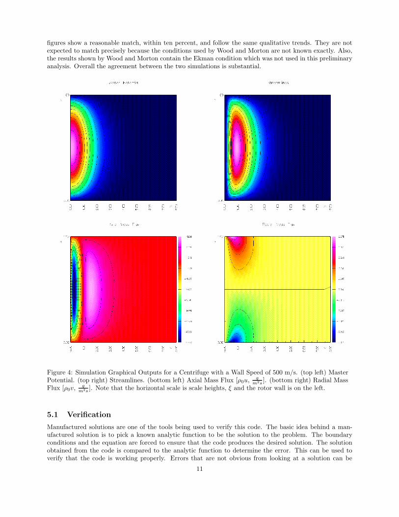
figures show a reasonable match, within ten percent, and follow the same qualitative trends. They are notexpected to match precisely because the conditions used by Wood and Morton are not known exactly. Also,the results shown by Wood and Morton contain the Ekman condition which was not used in this preliminaryanalysis. Overall the agreement between the two simulations is substantial.

Figure 4: Simulation Graphical Outputs for a Centrifuge with a Wall Speed of 500 m/s. (top left) MasterPotential. (top right) Streamlines. (bottom left) Axial Mass Flux [ρ0u,

gm2s ]. (bottom right) Radial Mass

Flux [ρ0v,g

m2s ]. Note that the horizontal scale is scale heights, ξ and the rotor wall is on the left.

5.1 Verification

Manufactured solutions are one of the tools being used to verify this code. The basic idea behind a man-ufactured solution is to pick a known analytic function to be the solution to the problem. The boundaryconditions and the equation are forced to ensure that the code produces the desired solution. The solutionobtained from the code is compared to the analytic function to determine the error. This can be used toverify that the code is working properly. Errors that are not obvious from looking at a solution can be

11

Figure 5: Streamlines for a Centrifuge with varying Wall Speed. (left) 400 m/s. (middle) 500 m/s. (right)700 m/s. Note that the horizontal scale is scale heights, ξ, which are a relative term that varies with thewall speed. If one were to do the graphs with absolute radial position on the horizontal scale they wouldappear essentially the same, all with the fluid motion occurring at the rotor wall. Note that the rotor wallis on the left.

0 1 2 3 4 5 6 7 8−70

−60

−50

−40

−30

−20

−10

0

10

20

30

Scale Heights

Axi

al M

ass

Flu

x

Axial Mass Flux at y/y0 = 0.5

400 m/s500 m/s700 m/s

0 1 2 3 4 5 6 7 8−70

−60

−50

−40

−30

−20

−10

0

10

20

30

Scale Heights

Axi

al M

ass

Flu

x

Axial Mass Flux at y/y0 = 0.25

400 m/s500 m/s700 m/s

Figure 6: (left) Axial Mass Flux at 0.5η1. (right) Axial Mass Flux at 0.25η1. The rotor wall is on the left.

12

revealed by techniques such as checking actual error convergence rates to see if they match the intendedrates.

Figure 7: Exact Solutions Used for Convergence Study. (left) Polynomial Function. (middle) TrigonometricFunction. (right) Pulse Function.

For each of the given convergence tables in Table 5, the convergence rate was approximated using a leastsquares fit of the log average grid spacing vs. the log of the maximum absolute error. They are each fromthe the 500 m/s wall speed case evaluated on the actual computational grid shown in Figure 3.

5.2 Validation

Reliable experimental data is difficult to obtain and is not expected to be available for validation. Areasonable amount of information is known about the flow inside a gas centrifuge to use physical insight tovalidate the code. One of the features that is expected is a weak countercurrent flow. This flow pattern iseasily seen in the streamline of Figure 5. Also by looking at the mass flux, which is the velocity multipliedby the density, one can verify that the radial component of the flow is strongest at the top and bottom ofthe machine. The flow has an equal and opposite velocity at the top and bottom of the machine. A similarphenomenon can be observed in the case of axial mass flux, however in that case the magnitudes differ due tothe density variation. One could integrate over the flow area to verify that the net flow rate is zero. Figure 4illustrates both of the above mentioned flow patterns.

5.3 Known Errors

There are still several areas of work that are needed to complete this project. While a fourth order accuratescheme is being used, the rate of convergence given by the manufactured solution does not match the expectedvalue. The maximum error values obtained are very large which is a cause for concern. As the three equationsare all coupled, error propagates through each one of the components and can become very large as shownin Figure 8. It appears that the largest error is located at the corners as is often the case.

The simulation behaved as expected in the 1-D radial case yet has had difficulty incorporating the axialderivative terms. This error is reduced as the wall speed increases since a higher wall speed results in a lowervalue of the constant term in front of the second axial derivative.

Another difficulty is that occasionally the external grids that are loaded into the simulation are notrecognized by the Overture database. This is easily fixed by re-creating one of the grids.

6 Conclusion

While there still remains work to be done a reasonable baseline solution has been obtained for the totalreflux case. The results obtained in this simulation are in reasonable agreement with the results obtained byWood and Morton. Further work to eliminate the corner errors and to achieve the desired order of accuracyis required. Once this is done greater complexity can be introduced.

13

h |χ− χe|∞ |ϕ− ϕe|∞ |%− %e|∞0.40 2.89e+03 9.41e+05 3.37e+080.20 1.40e+02 3.63e+04 3.12e+070.10 1.08e+01 3.32e+03 2.89e+060.05 7.50e+00 2.30e+02 2.00e+05

rate 3.95 3.94 3.56

Table 3: Convergence Rate Test: Polynomial Function.

h |χ− χe|∞ |ϕ− ϕe|∞ |%− %e|∞0.40 7.61e+01 4.08e+04 1.55e+070.20 1.50e-00 5.34e+02 1.80e+050.10 1.27e-01 6.24e-00 2.63e+040.05 5.63e-02 2.71e+01 2.36e+04

rate 3.48 3.81 3.09

Table 4: Convergence Rate Test: Trigonometric Function.

h |χ− χe|∞ |ϕ− ϕe|∞ |%− %e|∞0.40 5.00e-03 7.15e-02 1.07e+010.20 3.17e-04 3.83e-03 5.26e-010.10 2.24e-05 2.53e-04 3.75e-020.05 2.58e-06 1.73e-05 2.41e-03

rate 3.66 4.00 4.02

Table 5: Convergence Rate Test: Pulse Function.

14

Figure 8: Error From Manufactured Solution Test. (top) Polynomial Function. (middle) TrigonometricFunction. (bottom) Pulse Function. (left column) χ error. (middle column) ϕ error. (right column) %error. Note that the horizontal scale is scale heights, ξ.

15

7 Future Work

Once the current difficulties with incorporating the axial derivative term are solved there are a variety ofareas in which further progress can be made. A logical first step would be to replace the slip condition atthe top and bottom with the Ekman condition. This will provide insight into just how much of an effectthe Ekman condition has on the final solution. The results from Wood and Morton are also available forverification. Once the Ekman condition is implemented, the code should be modified to accept overlappinggrids. This will allow the user to concentrate points at areas of interest, which is especially of interest whenthere are feed, product, and waste streams. An overlapping grid has the advantage of using a coarse gridfor speed over the entire domain and finer grids over only the areas of interest. It would also be instructiveto run the simulation with several different sizes for the solution space to see what impact the size of thecomputational space has on the solution. A similar task would be to perform a sensitivity study for thedifferent variables in Onsager’s Master Equation. The solution is currently obtained with scale heights asthe radial scale, it is desirable to also get the solution in physical space, especially for comparison with othersimulations.

Once the code is working with overlapping grids, it is desirable to move from the highly idealized totalreflux case to a more realistic case with feed, product, and waste streams. This scenario is much closerto what actually occurs inside a gas centrifuge and introduces its own complexities, such as how to handlethe different properties of the product and waste streams. One could also add scoop drive and end capthermal drive to the wall thermal drive. This would most easily be accomplished by including source andsink terms as done by Wood and Morton[2]. Another useful tool would be to have an eigenfunction solutionfor comparison with the numerical one. This provides an additional check to make sure that the code isworking correctly.

Separative Work (SWU) is the quantity that is most desired for the analysis of a gas centrifuge. TheSWU and feed rate are the two most important variables for doing calculations for centrifuge cascades, whichare always used in practice. To obtain the SWU, the species equation must also be solved. It would also beuseful to modify the code to solve for the temperature field. The Cohen M-factor provides a measure of howdifferent a centrifuge is operating from ideal at each point in the axial direction.

One could also make a graphical user interface (GUI) that would make it easier for a user to customize asimulation. For example, one could quickly run a simulation of the total reflux case and then compare thatsolution to the one obtained in the more realistic with feed case. This tool would make the code much easierfor a non-expert, as well as reduce the amount of time it takes to learn to use the program.

The results obtained from this program could be used as an initial guess for a more complex Navier-Stokescode. This would provide such a code with a reasonable estimate of the flow field in the axisymmetric plane.It remains to be determined whether such a high-fidelity Navier-Stokes simulation is needed.

References

[1] Donald R. Olander. The theory of uranium enrichment by the gas centrifuge. Progress in Nuclear Energy,8:1–31, 1981.

[2] Houston G. Wood and J.B. Morton. Onsager’s pancake approximation for the fluid dynamics of a gascentrifuge. Journal of Fluid Mechanics, 101(1):1–31, 1980.

A Pseudocode for Simulation

This simulation was run from the file ”Onsagerspancakeapproxtotalrefluxcase.C” It was written in C++using the Overture library.

Pseudocode for ”Onsagerspancakeapproxtotalrefluxcase.C”1. Include relevant libraries2. Choose whether to plot output (set doplot to 1 for yes, 0 for no)3. Choose whether to recordsteps in the plot window (recordsteps to 0 for no, 1 for yes)4. Ask user for inputs (wall speed, grid file name, number of horizontal grid points, number of vertical grid

16

points, forcing option).5. Load grid6. Define Simulation parameters7. Update mapped grid properties (unnecessary if grid is loaded, required if a grid is generated within file)8. Create forcing functions9. Initialize coefficient matrix: coeff10. Initialize grid functions11. Name grid functions12. Define mapped grid operators13. Define coefficient matrix over entire computational space14. Define ghostlines for coefficient matrix15. Define boundary conditions for coefficient matrix16. Initialize right hand side over the entire computational space17. Define right hand side on the boundaries18. Initialize solver19. Simultaneously solve the system of equations20. Extract streamlines21. Extract radial and axial mass flow rate22. Calculate error all over for twilight zone flows23. Find maximum error for each of the three equations (from system)24. Open plot window (if chosen above)25. Record steps in plot GUI (if chosen above)26. Plot master potential, error, streamlines, axial and radial mass flux (if chosen above)27. End

17