Int. J. Electron. Commun. (AEU) 58 (2004): 339–348http://www.elsevier.de/aeue

A New State-space-based Algorithm to Assess the Stability of theFinite-difference Time-domain Method for 3D Finite

Inhomogeneous Problems

Bart Denecker, Luc Knockaert, Frank Olyslager, and Daniël De Zutter

Abstract: The finite-difference time-domain (FDTD) method is anexplicit time discretization scheme for Maxwell’s equations. In thiscontext it is well-known that explicit time discretization schemeshave a stability induced time step restriction. In this paper, werecast the spatial discretization of Maxwell’s equations, initiallywithout time discretization, into a more convenient format, calledthe FDTD state-space system. This in turn allows us to derivea new algorithm in order to determine the stability limit of FDTDfor lossy, inhomogeneous finite problems. It is shown that a crucialparameter is the spectral norm of the matrix resulting from the spa-tial discretization of the curl operator. In a rectangular simulationdomain the time step upper bound can be calculated in closed formand results in a time step limit less stringent than the Courant con-dition. Finally, the validity of the technique is illustrated by meansof some pertinent numerical examples.

Keywords: Finite-difference time-domain, State-space, Maxwell’sequations, Stability condition

1. Introduction

The finite-difference time-domain (FDTD) method isa popular simulation technique to solve Maxwell’s equa-tions [1]. The standard technique uses, as a result ofspatial discretization, a uniform staggered so-called Yeegrid to discretize Maxwell’s curl equations. Subsequentlytime is discretized using an explicit method leading to anefficient leapfrog iteration scheme. This technique wasfirst presented in 1966 [2].

A consequence of using an explicit method, except e.g.in the Dufort-Frankel scheme for parabolic problems, isa time step restriction in general: for time steps chosentoo large, the values of the variables grow without boundleading to instability and unphysical results. The stabilitylimit, known as the Courant-Friedrichs-Lewy [3] condi-tion, in short the Courant condition, was presented in thecase of the two-dimensional wave equation in [4], andfor the first time in the context of Maxwell’s equationsin [5]. In this last paper it was calculated using the VonNeumann method, determining, as a function of the time

Received September 30, 2003. Revised November 25, 2003.

Department of Information Technology (INTEC), Ghent University,Sint-Pietersnieuwstraat41, B-9000 Gent, Belgium

Correspondence to: Luc Knockaert.E-mail: Luc.Knockaert@intec.ugent.be

step, the growth factor of the Fourier spatial modes in aninfinite lossless homogeneous medium. Later this analy-sis was extended to infinite lossy homogeneous media [6]and in [7] the instability of the FDTD algorithm at theso-called “Magic Time Step” in 1D and 2D was provedusing the Von Neumann method for infinite homogeneousmedia.

Although the FDTD method seems to be stable for in-homogeneous finite problems using the same time steplimit, this has not been proved up to now. Only recently [8,9] a new approach was presented to study the stabil-ity condition of the FDTD method. The FDTD iterationscheme is described using sparse matrices and the eigen-values of the iteration matrix are examined. In [8] thestability of nonorthogonal FDTD methods was investi-gated. In [9], it was shown, working with a uniform grid,that a time step limit certainly exists for inhomogeneousfinite problems and that this limit was related to the larg-est eigenvalue of a sparse matrix. A useful bound couldbe derived; however, for 2D problems, this bound was√

2 times more strict than the Courant limit. Later [10]the same author presented a result for homogeneous fi-nite 2D problems, showing a bound similar to the Courantlimit.

In this paper, we recast the spatial discretization ofMaxwell’s equations, initially without time discretization,into a more convenient format, called the FDTD state-space system. This in turn allows us to derive a new al-gorithm in order to determine the stability limit of FDTDfor lossy, inhomogeneous finite problems. The new algo-rithm shows that the stability limit for the FDTD methodis independent of the losses in the problem. It is further-more shown that a stability limit for homogeneous mediais also a sufficient, albeit not necessary, condition for in-homogeneous problems. For a 3D rectangular domain thislimit can be calculated in closed form, leading to a use-ful stability condition for 3D lossy inhomogeneous finiteproblems.

In Section 2 the FDTD state-space system is ana-lyzed with special emphasis on some key properties of thesparse matrices involved. In Section 3 the time discretizedversion of the FDTD state-space system is presented andit is shown that a stability limit, depending only on thespectral norm‖K‖2, presents a sufficient condition inde-pendent of losses and (an)isotropic inhomogeneities. InSection 4,‖K‖2 is calculated for a rectangular simula-tion domain and the final result is discussed in Section 5and compared to the well known Courant limit. Finally,

1434-8411/04/58/05-339 $ 30.00/0

340 Bart Denecker et al.: A New State-space-based Algorithm to Assess the Stability of the Finite-difference. . .

in Section 6, some numerical results are presented thatclearly illustrate the usefulness of our approach.

2. The FDTD state-space system

Consider a finite FDTD simulation domain terminated byperfect electric conductors (PEC). The FDTD equationsfor a medium with relative permittivityεr, relative per-meabilityµr, electric conductivityσe and magnetic con-ductivity σm take on the following form:

εrdex|i+1/2, j,k

dτ= − 1

∆zhy|i+1/2, j,k+1/2

+ 1

∆zhy|i+1/2, j,k−1/2

+ . . .−σe R0ex|i+1/2, j,k (1)

µrdhy|i+1/2, j,k+1/2

dτ= 1

∆zex|i+1/2, j,k

+ . . .− σm

R0hy|i+1/2, j,k+1/2

(2)

where we kept the time derivatives and only discretizedthe spatial coordinates. We have also normalized the mag-netic field by a factorR0 = √

µ0/ε0 and the normalizedtime τ is defined asτ = c0t, wherec0 = 1/

√ε0µ0 is the

speed of light. The grid steps are∆x,∆y and∆z and wehave used the traditional FDTD index notation.

It is seen that there is a reciprocity between equations(1) and (2); e.g. in (1) the coefficient ofhy|i+1/2, j,k+1/2

is−1/∆z while in (2) the coefficient ofex |i+1/2, j,k is 1/∆z.By imposing PEC boundaries, this mutual coupling prop-erty is valid for each equation throughout the entire simu-lation domain. This was first observed in [11] and in [12]and called reciprocity in [13]. It was also exploited in [14].Here, we call this mutual coupling property spatial reci-procity, since it is related to the way the spatial domain isdiscretized. This allows us, by grouping the electric fieldvariables in a vectore, and the magnetic field variables ina vectorh, to write down the FDTD equations (1) and (2)in block state space form as follows:[

Dε 00 Dµ

][eh

]= −

[Dσe K−KT Dσm

][eh

](3)

or, still more compactly [15] as

Cx = −Gx (4)

wherex is shorthand notation fordx/dτ. The off-diagonalblocks ofC are zero and the diagonal blocks,C11 = Dε

andC22 = Dµ, are diagonal matrices containing the rela-tive permittivity of each electric field variable or the rela-tive permeability of each magnetic field variable respec-tively. Each diagonal element ofDε is strictly positive andmoreover each diagonal element has at least the value 1:

[Dε]rr ≥ 1 ∀r (5)

This is also true forDµ:[Dµ

]rr ≥ 1 ∀r (6)

These relations also hold for anisotropic media for whichthe principal axes coincide with the coordinate axes.

The diagonal blocks inG, are diagonal matrices andcontain the losses corresponding to each field variable:G11 = Dσe contains the normalized electric losses, andG22 = Dσm , contains the normalized magnetic losses.Each diagonal element ofDσe and ofDσm is non-negative:[

Dσe

]rr ≥ 0 ∀r (7)[

Dσm

]rr ≥ 0 ∀r (8)

thereforeDσe and Dσm are positive semi-definite. In (3)the spatial reciprocity manifests itself by considering theoff-diagonal blocks ofG: blockG21 = −KT , representingthe relations between the magnetic and the electric fieldvariables, is the skew transpose of blockG12 = K, rep-resenting the relations between the electric and magneticfield variables.

As will become clear later on, the stability of theFDTD algorithm depends on the matrixK in (3). It can bewritten down explicitly when the simulation domain is therectangular box of Fig. 1. The simulation domain is termi-nated by perfect electric (PEC) conductors and hence thetangential electric fields and normal magnetic fields at theboundaries are zero, i.e.:• ey = ez = 0, hx = 0 atx = 0 andx = nx∆x• ex = ez = 0, hy = 0 at y = 0 andy = ny∆y• ex = ey = 0, hz = 0 at z = 0 andz = nz∆z

One can show that the explicit expression for the ma-trix K is as follows:

K =

0INx ⊗ Iny ⊗ WNz

∆z

−INx ⊗ WNy∆y

⊗ Inz

−Inx ⊗ INy ⊗ WNz∆z

Inx ⊗ WNy∆y

⊗ INz

0 −WNx∆x

⊗ Iny ⊗ INzWNx∆x

⊗ INy ⊗ Inz 0

(9)

Fig. 1. Rectangular simulation domain withnx ×ny ×nz Yee cells.

Bart Denecker et al.: A New State-space-based Algorithm to Assess the Stability of the Finite-difference. . . 341

with Nα = nα − 1 for α = x, y, z and where the matrixWr ∈ Rr×(r+1) is given by

Wr =

1 −1

1. . .

. . . −11 −1

(10)

with Ir the identity matrix of dimensionr. The Kroneckerproduct⊗ is defined in the Appendix.

3. Time discretization of the FDTDstate-space system

In this section the FDTD time discretization of the state-space system (3) will be discussed, and stability can onlybe assured for limited time steps, with a limit related tothe spectral norm‖K‖2. For the moment we do not makeany assumptions concerning the shape of the simulationdomain. If we use the standard FDTD central differenceapproximations we obtain:(

Dε

∆τ

+ Dσe

2

)e|n+1/2

=(

Dε

∆τ

− Dσe

2

)e|n−1/2 −Kh|n(

Dµ

∆τ

+ Dσm

2

)h|n+1 −KT e|n+1/2

=(

Dµ

∆τ

− Dσm

2

)h|n (11)

where the superscripts represent the normalized time, i.e.n representsτ = n∆τ . Just as the field variables insideeach cell are interleaved, the field variables are updated inan alternating way, i.e. at different moments in time:• atτ = n∆τ , the magnetic field variables are updated• at τ = (n +1/2)∆τ , the electric field variables are up-

dated.Old values at previous time instants do not need tobe stored, therefore this alternating scheme is calleda leapfrog iteration scheme. This can be written in matrixform as:

(E+F)x|n+1 = (E−F) x|n (12)

where

E =[∆−1

τ Dε − 12 K

− 12 KT ∆−1

τ Dµ

](13)

F =[ 1

2 Dσe12 K

− 12 KT 1

2 Dσm

](14)

x|n =[

e|n−1/2

h|n]

For each time stepy = (E−F)x|n is calculated and(E+F)x|n+1 = y is solved forx|n+1. Since(E−F) and(E+F)are sparse upper triangular and lower triangular matrices,this can be implemented very efficiently. Of course, this isjust one of the main advantages of the FDTD method.

The stability of the FDTD equations is related to thespectral radius, defined as the maximum of the absolutevalues of the eigenvalues, of the iteration matrix

(E+F)−1 (E−F) (15)

Each eigenvalue,γ , of (15) is related to the eigenvalue,λ,of E−1F by means of the bilinear transformation

γ = 1−λ

1+λ(16)

and the condition,|γ | ≤ 1, to ensure stability, is equivalentwith the condition Re[λ] ≥ 0.

The eigenvalueλ and the associated eigenvectorz sat-isfy the relation

Fz = λEz (17)

By left multiplying (17) withzH , the Hermitian transposeof the eigenvectorz, this becomes:

zH Fz = λzH Ez (18)

The Hermitian transpose of (18) is:

zH FT z = λ∗zH ET z (19)

where we took into account thatE and F are real ma-trices and thatE is symmetric such thatFH = FT andEH = ET = E. Adding (18) and (19) yields:

1

2zH(F+FT)z = Re(λ)zH Ez (20)

Note that

F+FT =[

Dσe 00 Dσm

](21)

is a diagonal matrix with no negative entries, i.e. a positivesemi-definite matrix. This ensures that the left hand sideof (20) is real and non-negative. With this result, it suf-fices to determine in whichcase the symmetric matrixEis positive definite, as from (20) it follows that in thatcase Re(λ) ≥ 0. Therefore only the matrixE determinesthe stability of the FDTD method, and (13) shows thatEdoes not depend on the conductivitiesσe, σm . Hence it isclear that losses do not play a role regarding the stabil-ity of the FDTD method. Thisis in agreement with [6],where based on the Von Neumann analysis for homoge-neous media, it was shown that, when using central dif-ference approximations, losses do not affect the stabilityconstraint. Here we have extended this conclusion to finiteinhomogeneous media. MatrixE must be positive definite

342 Bart Denecker et al.: A New State-space-based Algorithm to Assess the Stability of the Finite-difference. . .

in order to have a stable algorithm. Suppose, as a first step,that the medium is vacuum, i.e.

E =[∆−1

τ In1 − 12 K

− 12 KT ∆−1

τ In2

](22)

Consider the singular value decomposition ofK ∈Rn1×n2,with n1 = dim[e] andn2 = dim[h]:

K = UT �V (23)

Here� ∈ Rn1×n2, U ∈ Rn1×n1 andV ∈ Rn2×n2, and bothU andV are orthogonal matrices:UT U = UUT = In1 andVT V = VVT = In2. Matrix � has only non-zero elem-ents on the diagonal and each of these elements,sp forp = 1, . . . , n1, is called a singular value i.e.

�pq ={

sp if p = q0 else

(24)

Hence we can put

E =[

UT 00 VT

][∆−1

τ In1 − 12 �

− 12 � T ∆−1

τ In2

][U 00 V

](25)

implying that the eigenvalues ofE are equal to the eigen-values of [

∆−1τ In1 − 1

2 �

− 12 � T ∆−1

τ In2

](26)

Supposingn1 ≤ n2, which is the case for the rectangularsimulation domain in Fig. 1 (a similar reasoning is pos-sible forn1 > n2 and leads to an identical result), we candefine a permutation matrixP

Ppq =

1 p = r, q = 2r −1 for r = 1, . . . , n1

1 p = r +n1, q = 2r for r = 1, . . . , n1

1 p = q = r for r = 2n1 +1, . . . , n1 +n2

0 else(27)

showing that (26) is similar to a block diagonal matrix:[∆−1

τ In1 − 12 �

− 12 � T ∆−1

τ In2

]= P � PT (28)

where� hasn1 blocks of size 2×2, and (n2 −n1) times1/∆τ on the diagonal:

� =diag

([1

∆τ− s1

2

− s12

1∆τ

], . . . ,

[1

∆τ− sn1

2

− sn12

1∆τ

],

1

∆τ

, . . . ,1

∆τ

)

SinceE is similar to� , the eigenvalues are identical. Theeigenvalues of� are 1/∆τ with multiplicity (n2 −n1) andthe eigenvalues of the diagonal blocks, i.e.

λ

([1

∆τ− sp

2

− sp2

1∆τ

])= 1

∆τ

± sp

2for p = 1, . . . , n1 (29)

All these eigenvalues are strictly positive when∆τ < 2/spfor all sp or

∆τ = c0∆t

∆<

2

s(30)

where s = max(sp). Equation (30) ensures the positivedefiniteness ofE and the stability of the FDTD method.On the contrary when (30) is violatedE will not be pos-itive definite and the FDTD method becomes unstable.Sinces = max(sp) = ‖K‖2 [16], (30) can also be writtenas:

∆τ <2

‖K‖2(31)

When condition (30) is satisfied, the matrix (22) ispositive definite for vacuum. Making use of the blockstructure ofE, this is equivalent to the statement that foreachzT = [zT

e zTh ]:

1

∆τ

zTe ze − 1

2zT

e Kzh − 1

2zT

h KT ze + 1

∆τ

zTh zh > 0 (32)

By exploiting (5), the following inequalities hold foreveryz:

zTe Dεze ≥ zT

e ze

zTh Dµzh ≥ zT

h zh

Therefore, when (32) is satisfied, the following inequalityalso holds:

1

∆τ

zTe Dεze − 1

2zT

e Kzh − 1

2zT

h KT ze + 1

∆τ

zTh Dµzh > 0

(33)

and hence the matrixE of (13) is positive definite, or inother words, the algorithm is stable, independently of thematerials used inside the simulation domain provided (30)is satisfied.

Summarized, it can be stated that the stability condi-tion is only determined by the largest singular value,S,of K satisfying the condition (30). In [9], for the losslesscase, a necessary and sufficient condition for stability wasgiven:

∆τ <2

ρ(34)

whereρ is the spectral radius of the matrix[0 D−1/2

ε KD−1/2µ

−D−1/2µ KT D−1/2

ε 0

](35)

whereD−1/2ε andD−1/2

µ are easily calculated sinceDε andDµ are diagonal matrices with strictly positive diagonalelements (5). ForDε = I andDµ = I, or in other wordsfor vacuum, this is the same as (30). It should be stressed

Bart Denecker et al.: A New State-space-based Algorithm to Assess the Stability of the Finite-difference. . . 343

that we have shown that result (30) is also sufficient forstability of inhomogeneous problems.

Now that we have derived the stability condition (30)or (31) and before expliciting the stability condition fora rectangular region, we want to emphasize that if (30) issatisfied for free space, we have shown that stability re-mains guaranteed when introducing material of any type.However, (30) is sufficient but not always necessary (aswill be shown in one example in Section 8), i.e. it maywell be that when introducing material, a larger time stepthan the one given by (30) still leads to a stable iterationscheme. Remark however that introducing losses will notallow for a larger time step.

The obtained result can indeed be generalized as fol-lows. Suppose that theεr andµr-values of the materialsatisfy:

εr ≥ εr,min

µr ≥ µr,min (36)

This would in particular be the case for a homogeneousmaterial with parametersεr andµr . It now suffices to re-placec0 andR0 by c andRc given by

c = 1√ε0µ0

1√εr,min, µr,min

Rc =√

µ0

ε0

õr,min

εr,min(37)

and to repeat the complete analysis, to come to the conclu-sion that (30) remains valid, implying that the actual timestep∆t is now larger asc < c0.

4. Singular values of K

In this section the singular values ofK (9) will be deter-mined when the simulation domain is a rectangular box,see Fig. 1. First of all consider the singular value decom-position ofWα/∆α:

1

∆α

WNα = UTα�αVα (38)

for α = x, y, z, whereWNα , �α ∈ RNα×nα , Uα ∈ RNα×Nα

andVα ∈ Rnα×nα and keeping in mind thatUα andVα areorthogonal.

Making use of the singular value decomposition of thedifferentW-matrices, and some readily established prop-erties of the Kronecker product, see the Appendix,K is:

K = UT1 �1V1 (39)

where

UT1 =

VT

x ⊗UTy ⊗UT

z 0 00 UT

x ⊗VTy ⊗UT

z 00 0 UT

x ⊗UTy ⊗VT

z

�1 =[ 0

INx ⊗ Iny ⊗�z−INx ⊗� y ⊗ Inz

−Inx ⊗ INy ⊗�z Inx ⊗� y ⊗ INz

0 −�x ⊗ Iny ⊗ INz

�x ⊗ INy ⊗ Inz 0

(40)

V1 =[

Ux ⊗Vy ⊗Vz 0 00 Vx ⊗Uy ⊗Vz 00 0 Vx ⊗Vy ⊗Uz

]

BothU1 andV1 are orthogonal matrices,UT1 U1 = U1UT

1 =In1 andVT

1 V1 = V1VT1 = In2, therefore the singular values

of K are equal to the singular values of�1. As a nextstep two permutation matrices can be introduced, the firstpermutation matrixP rearranging the rows of�1, the sec-ond permutation matrixQ rearranging the columns of�1.This results in transforming�1 to �2:

K = UT1 PT �2QV1 (41)

such that�2 is a block diagonal matrix, where the blockson the diagonal are not necessarily square, but the elem-ents above and below these blocks are zero. For brevityPandQ are not given, but the idea is similar to what wasdone in (28). The resulting block diagonal matrix is of thefollowing form:

�2 = diag

{[0 −sz,k sy, j

sz,k 0 −sx,i−sy, j sx,i 0

], . . . ,

[−sz,k sy, j], . . . ,

[sz,k −sx,i

], . . . ,

[−sy, j sx,i]}

for i = 1, . . . , Nx , j = 1, . . . , Ny and k = 1, . . . , Nz .Wheresx,i is thei th singular value of�x , sy, j is the j th sin-gular value of� y andsz,k is thekth singular value of�zappearing in (40). Since bothU1 andP are orthogonal andhave the same dimension, their productPU1 is orthogonal.The same remark can be made forQV1.

In this way, the problem of finding the singular valuesof K has been simplified to finding the singular values of�2. The singular values of�2 are the singular values ofeach of the block matrices on the diagonal. For both typesof matrices the singular values are:

s

([0 −c bc 0 −a

−b a 0

])={√

a2 +b2 + c2,√

a2 +b2 + c2, 0}

(42)

s([

a b])=

√a2 +b2 (43)

wheres(A) lists the singular values ofA. From this resultit is clear that the spectral norm ofK is given by:

‖K‖2 =√

s2x + s2

y + s2z (44)

344 Bart Denecker et al.: A New State-space-based Algorithm to Assess the Stability of the Finite-difference. . .

where

sx = maxi

(sx,i) = ‖�x‖2 (45)

sy = maxj

(sy, j) = ∥∥� y

∥∥2 (46)

sz = maxk

(sz,k) = ‖�z‖2 (47)

Finally we need to determine the largest singular valueof Wr (10). The singular values ofWr , as can be seen byconsidering the singular value decomposition ofWr , cor-respond to the positive square root of the eigenvalues ofWrWT

r :

WrWTr =

2 −1−1 2 −1

−1 2. . .

. . .. . . −1−1 2

(48)

and from [17], it is found that these eigenvalues are:

λs = 2+2 cos

(pπ

r +1

)= 4 cos2

(pπ

2(r +1)

)s = 1, . . . , r (49)

therefore:

Sα = max(�α) = 2

∆α

cos(

π

2nα

)for α = x, y, z

(50)

Introducing this result in (44), the largest singular value ofK becomes:

S =√4

∆2x

cos2(

π

2nx

)+ 4

∆2y

cos2(

π

2ny

)+ 4

∆2z

cos2(

π

2nz

)(51)

5. Stability criterion

Combining (30) and (51) yields a stability condition fora 3-D finite inhomogeneous lossy FDTD scheme:

∆τ <

1

c0

√1

∆2x

cos2(

π2nx

)+ 1

∆2y

cos2(

π2ny

)+ 1

∆2z

cos2(

π2nz

)(52)

Note that the validity of (52) includes anistropic media.Based on the fact that:

cos2(

π

2nx

)< 1 (53)

it can be concluded that result (52) is less stringent thanthe well known result [5] obtained via the Von Neumannmethod, i.e.

∆τ ≤ 1

c0

√1

∆2x+ 1

∆2y+ 1

∆2z

(54)

which is better known as the Courant limit. From (52), itcan be observed that for an infinitely large grid our resultapproaches the Courant condition (54) since cos2(π/2nα)approaches one fornα → ∞. It is important to note how-ever that our result has been proved for finite lossy inho-mogeneous problems.

A similar algebraic approach was presented recentlyfor 2-D systems in [10], the analysis was limited to homo-geneous and lossless media.

6. Numerical examples

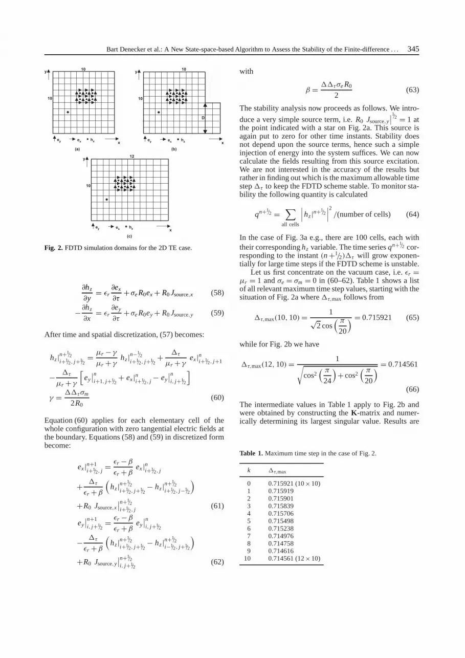
In this section the derived stability conditions are illus-trated by means of two-dimensional (2D) FDTD simula-tions. The advantage of 2D examples over 3D ones, is thatthe set of relevant equations is greatly simplified whilekeeping all the essential features of the 3D case. In the 2Dcase all fields are independent of one coordinate (sayz)and the 2D problem falls apart into a TM-case for thehx,hy andez components and a TE-case for theex, ey andhzcomponents. The example that we will treat here is thatof the TE-case for the rectangular andL-shaped regionsof Fig. 2.

We will start with the rectangular region of Fig. 2a forwhichnx = 10, ny = 10 with∆x = ∆y = ∆.

According to (52), the FDTD time step must satisfy

∆τ = c0∆t

∆<

1√cos2

(π

2nx

)+cos2

(π

2ny

) (55)

The field components are arranged as shown in a part ofFig. 2a with the tangential electric fields put to zero on theboundary. Next, wewill investigate how the stability con-dition evolves when going from the situation of Fig. 2a tothat of Fig. 2c wherenx = 12, ny = 10 through intermedi-ateL-shaped situations, one of which is shown in Fig. 2b.Remark that for Fig. 2c, (55) again applies while for theintermediate situations the maximum singular valuesmaxof K will have to be determined numerically. For theL-shaped cases we then have

∆τ = c0∆t

∆<

2

smax(56)

The field equations which govern the problem are:

∂ey

∂x− ∂ex

∂y= −µr

∂hz

∂τ− σm

R0hz (57)

Bart Denecker et al.: A New State-space-based Algorithm to Assess the Stability of the Finite-difference. . . 345

Fig. 2. FDTD simulation domains for the 2D TE case.

∂hz

∂y= εr

∂ex

∂τ+σe R0ex + R0Jsource,x (58)

−∂hz

∂x= εr

∂ey

∂τ+σe R0ey + R0Jsource,y (59)

After time and spatial discretization, (57) becomes:

hz|n+1/2i+1/2, j+1/2

= µr −γ

µr +γhz|n−1/2

i+1/2, j+1/2+ ∆τ

µr +γex|ni+1/2, j+1

− ∆τ

µr +γ

[ey

∣∣ni+1, j+1/2

+ ex|ni+1/2, j − ey

∣∣ni, j+1/2

]γ = ∆∆τσm

2R0(60)

Equation (60) applies for each elementary cell of thewhole configuration with zero tangential electric fields atthe boundary. Equations (58) and (59) in discretized formbecome:

ex|n+1i+1/2, j

= εr −β

εr +βex |ni+1/2, j

+ ∆τ

εr +β

(hz|n+1/2

i+1/2, j+1/2− hz|n+1/2

i+1/2, j−1/2

)+R0 Jsource,x

∣∣n+1/2i+1/2, j (61)

ey

∣∣n+1i, j+1/2

= εr −β

εr +βey

∣∣ni, j+1/2

− ∆τ

εr +β

(hz|n+1/2

i+1/2, j+1/2− hz|n+1/2

i−1/2, j+1/2

)+R0 Jsource,y

∣∣n+1/2i, j+1/2

(62)

with

β = ∆∆τσe R0

2(63)

The stability analysis now proceeds as follows. We intro-

duce a very simple source term, i.e.R0 Jsource,y

∣∣1/2 = 1 atthe point indicated with a star on Fig. 2a. This source isagain put to zero for other time instants. Stability doesnot depend upon the source terms, hence such a simpleinjection of energy into the system suffices. We can nowcalculate the fields resulting from this source excitation.We are not interested in the accuracy of the results butrather in finding out which is the maximum allowable timestep∆τ to keep the FDTD scheme stable. To monitor sta-bility the following quantity is calculated

qn+1/2 =∑

all cells

∣∣∣hz|n+1/2

∣∣∣2 /(number of cells) (64)

In the case of Fig. 3a e.g., there are 100 cells, each withtheir correspondinghz variable. The time seriesqn+1/2 cor-responding to the instant(n +1/2)∆τ will grow exponen-tially for large time steps if the FDTD scheme is unstable.

Let us first concentrate on the vacuum case, i.e.εr =µr = 1 andσe = σm = 0 in (60–62). Table 1 shows a listof all relevant maximum time step values, starting with thesituation of Fig. 2a where∆τ,max follows from

∆τ,max(10, 10) = 1√2 cos

( π

20

) = 0.715921 (65)

while for Fig. 2b we have

∆τ,max(12, 10) = 1√cos2

( π

24

)+cos2

( π

20

) = 0.714561

(66)

The intermediate values in Table 1 apply to Fig. 2b andwere obtained by constructing theK-matrix and numer-ically determining its largest singular value. Results are

Table 1. Maximum time step in the case of Fig. 2.

k ∆τ,max

0 0.715921 (10×10)1 0.7159192 0.7159013 0.7158394 0.7157065 0.7154986 0.7152387 0.7149768 0.7147589 0.714616

10 0.714561 (12×10)

346 Bart Denecker et al.: A New State-space-based Algorithm to Assess the Stability of the Finite-difference. . .

Fig. 3. Stability measureqn+1/2 for the configuration of Fig. 2a.

given for 9 possible intermediate situations withD = k∆;k = 1, 2, . . . , 9 (in Fig. 2b,k = 5). Remark that the rel-evant∆τ,max value varies progressively between the ex-tremes fork = 0 andk = 10. Fig. 2 displaysqn+1/2 (64) asa function of discretized timen for the (10×10) config-uration of Fig. 2a (with∆τ,max given by (65)). The curvescorrespond with different values of the time step∆τ withp = ∆τ/∆τ,max. To normalize the results, we have firstcalculatedqn+1/2 for ∆τ = ∆τ,max and we have dividedall other results by the value ofqn+1/2 for this limitingcase by theq-value atn = 200. As can be seen fromFig. 2, this limiting case leads to a result which increaseswith time, to reach a maximum value of 1 (as a conse-quence of our normalization of the results). It can nowvery clearly be observed that time steps only by very lit-tle exceeding the maximum allowable time step, lead toexponentially unstable results, while just below the max-imum allowable time step the algorithm remains stable.A very much similar set of results (see Fig. 4) is obtainedfor the L-shaped situation of Fig. 2b(D = 5∆, ∆τ,max =0.715498). To further stress how the predicted stabilitylimit shows up in the numerical data, the curves of Fig. 4include two values ofp, namely p = 1.000001 andp =0.999999, which are closer to unity than the correspond-ing values of Fig. 2. It is seenthat the numerical resultsclearly confirm the theoretical derivations of the previoussections.

Fig. 4. Stability measureqn+1/2 for the configuration of Fig. 2b(D = 5∆).

Finally, just by way of example, we investigate theeffect of introducing material into the configuration ofFig. 2a. We do this in the following way. Starting from thevacuum case, the first row is filled with a non-conductingmaterial withεr = 1 andµr = 4. Next, the second row isfilled and so on until a fully homogeneous cross-section isagain obtained. We have proved that the FDTD algorithmwill remain stable when using (65), the vacuum result.However, as already explained, we have only proved thatrespecting (65) is sufficient but not necessary when intro-ducing material. Hence, in the presence of material, wehave determined the actual stability limit experimentallyby performing many FDTD solutions and by carefully ob-serving the behaviour ofqn+1/2 for large values of time.The obtained results are given in Table 2 under the form ofa multiplication factor with which the vacuum limit (65)has to be multiplied. As claimed theoretically, this factorindeed always exceeds 1. For the homogeneous case withεr = 1 andµr = 4, we refer to the remark at the end ofSection 5 and to (37). As the speed of light is now twotimes smaller than in the vacuum case, the multiplicationfactor must exactly become 2. This is also confirmed byour numerical experiment, but the gradual transition fromthe vacuum case to the fully filled cross-section certainlydoes not lead to a similar gradual increase in the mul-tiplication factor. To obtain the data in Table 2 with anaccuracy of 5 digits about 2000 time steps were necessary.

To conclude, the effect of losses is illustrated in Fig. 5and Fig. 6.

The displayed results are similar to the ones shownin Figs. 3 and 4. The configuration we consider is that ofFig. 2a (the 10×10 case) withεr = 1 andµr = 1.

However, half of the cross-section has been filled withmaterial with magnetic losses for whichγ = 1 in the caseof Fig. 5 andγ = 10 in the case of Fig. 6. We have retainedthree values forp and the results forqn+1/2 have nowbeen normalized with the values ofqn+1/2 at n = 200 forp = 1, i.e. ∆τ = ∆τ,max with ∆τ,max the free space valueof 0.715921. The numerical results confirm that stabilityis independent from losses. Although the three curves arevery close to each other for early time, they clearly sepa-rate when time increases with clear stability forp < 1.

Table 2. Maximum time step in the case of partial filling.

Rows filled ∆τ,max/∆τ,max,vacuum

0 0.999991 1.000612 1.002303 1.004724 1.008335 1.014076 1.024047 1.043688 1.091059 1.25261

10 1.99999

Bart Denecker et al.: A New State-space-based Algorithm to Assess the Stability of the Finite-difference. . . 347

Fig. 5. Stability measureqn+1/2 for the configuration of Fig. 2ahalf filled with conducting material withγ = 1.

Fig. 6. Stability measureqn+1/2 for the configuration of Fig. 2ahalf filled with conducting material withγ = 10.

7. Conclusion

We have presented a new algorithm to assess the stabilityof the FDTD method. It is based on the spatial discretiza-tion of Maxwell’s equations, initially without time dis-cretization, leading to an FDTD state-space system. Fromthe subsequent time discretization of the FDTD state-space system, a technique was derived to determine thestability limit for lossy, inhomogeneous finite problems.

This stability limit, related to the spectral norm of thediscretized curl operator, only depends on the grid of theFDTD method and is a sufficient condition independent ofinhomogeneous lossless media inside the problem. It hasalso been proved that the stability limit is not influencedby the insertion of electric or magnetic losses. For a rect-angular simulation domain this limit can be calculated andresults in a stability limit less strict than the Courant con-dition.

To give the reader a feeling about the way in whichthe derived time step stability limit manifests itself in nu-merical calculations, a 2D FDTD example was studied indetail. Both the effect of a change in shape of the simu-lation domain as well as the effect of introducing lossless

and lossy material are examined and the obtained resultsare fully consistent with the theory.

Acknowledgement. Part of the research reported inthis paper was supported by the CODESTAR-IST project.

Appendix

The Kronecker product ofB ∈ Rm×n and C ∈ Rp×q isgiven by

A = B⊗C =

b11C b12C . . . b1nCb21C b22C . . . b2nC

......

. . ....

bm1C bm2C . . . bmnC

(A1)

andA ∈ Rm p×nq , see [16]. This is am-by-n block matrixwhere block(i, j) is bijC. The following properties arereadily available [18]:

A⊗ (B⊗C) = (A⊗B)⊗C (A2)(A⊗B)(C⊗D) = (AC⊗BD) (A3)

(A⊗B)T = (AT ⊗BT ) (A4)

References

[1] Taflove, A.; Hagness, S. C.: Computational electrodynamics:The finite-difference time-domain method. Norwood, MA:Artech House, 2000.

[2] Yee, K. S.: Numerical solution of initial boundary value prob-lems involving maxwell’s equations in isotropic media. IEEETrans. Antennas Propagat.14 (1966), 302–307.

[3] Courant, R.; Friedrichs, K.; Lewy, H.: On the partial differ-ence equations of mathematical physics, (english translationof the original work, über die partiellen Differenzen Gle-ichungen der mathematischen Physik,math. ann. 100 (1928)32–74.). IBM Journal11 (1967), 215–234.

[4] Lewy, H.: On the convergence of solutions of differenceequations. – In: Studies and essays presented to R. Couranton his 60th birthday. Lewy, H. (ed.). New York: InterSciencePublishers Inc., 1948, 211–214.

[5] Taflove, A.; Brodwin, M. E.: Numerical solution ofsteady-state electromagnetic scattering problems usingthe time-dependent maxwell’s equations. IEEE Trans.Microwave Theory Tech.23 (1975), 623–630.

[6] Pereda, J. A.; Garcıa, O.; Vegas, A.; Prieto, A.: Numeri-cal dispersion and stability analysis of the FDTD techniquein lossy dielectrics. IEEE Microwave Guided Wave Lett.8(1998), 245–247.

[7] Min, M. S.; Teng, C. H.: The instability of the yee schemefor the “magic time step”. J. Comput. Phys.166 (2001), 418–424.

[8] Gedney, S. D.: Numerical stability of nonorthogonal fdtdmethods. IEEE Trans. Antennas Propagat.48 (2000), 231–239.

[9] Remis, R. F.: On the stability of the finite-difference time-domain method. J. Comput. Phys.163 (2000), 249–261.

348 Bart Denecker et al.: A New State-space-based Algorithm to Assess the Stability of the Finite-difference. . .

[10] Remis, R. F.: Global form of the 2d finite-difference maxwellsystem and its symmetry properties. Proceedings 2002 IEEEAntennas and Propagation Symp., San Antonio Texas, 2002.624–627.

[11] Railton, C. J.; Craddock, I. J.; Schneider, J. B.: Improved lo-cally distorted CPFDTD algorithm with provable stability.Electronics Letters31 (1995), 1585–1586.

[12] Thoma, P.; Weiland, T.: A consistent subgridding scheme forthe finite difference time domain method. J. Numer. Model.-Electron. Netw. Device Fields9 (1996), 359–374.

[13] Krishnaiah, K. M.; Railton, C. J.: Passive equivalent circuitof FDTD: an application to subgridding. Electron. Lett.33(1997), 1277–1278.

[14] Remis, R. F.; van den Berg, P. M.: A modified algorithmfor the computation of transient electromagnetic wavefields.IEEE Trans. Microwave Theory Tech.45 (1997), 2139–2149.

[15] Denecker, B.; Olyslager, F.; Knockaert, L.; De Zutter, D.:Generation of FDTD subcell equations by means of reducedorder modeling. IEEE Trans. Antennas Propagat.51 (2003),1806–1817.

[16] Golub, G. H.; Van Loan, C. F.: Matrix computations. London:Johns Hopkins University Press, 1996.

[17] Smith, G. D.: Numerical solution of partial differential equa-tions: Finite difference methods. Oxford: Clarendon Press,1985.

[18] Granata, J.; Conner, M.; Tolimieri, R.: Recursive fast algo-rithms and the role of the tensor product. IEEE Trans. SignalProcessing40 (1992), 2921–2930.

Bart Denecker was born in Roeselare,Belgium, in 1975. He received the elec-trotechnical engineering degree and thePh. D. degree from the Department of In-formation Technology, Ghent University,Belgium, in July, 1998 and 2003, respec-tively.His primary research concerns the finite-difference time-domain method.

Luc Knockaert received the M. Sc. De-gree in physical engineering, M. Sc. De-gree in telecommunications engineeringand Ph. D. Degree in electrical engineer-ing from Ghent University, Belgium, in1974, 1977, and 1987, respectively.From 1979 to 1984 and from 1988 to 1995he was working in North-South cooper-ation and development projects at the Uni-versities of Congo (formerly Zaire) andBurundi. He is presently a guest profes-

sor and senior researcher at INTEC-IMEC. His current interestsare the application of statistical and linear algebra methods in sig-nal identification, sampling theory, matrix compression, reducedorder modeling and the use of integral transforms in electromag-netic problem solving. As author or co-author he has contributedto more than 40 international peer-reviewed journal papers.

Dr. Knockaert is a member of ACM, SIAM and a senior memberof IEEE.

Frank Olyslager was born in 1966. Hereceived the electrical engineering and Ph.D. degrees from Ghent University, Bel-gium, in 1989 and 1993, respectively.At present he is a full professor of elec-tromagnetics at Ghent University. His re-search concerns different aspects of the-oretical and numerical electromagnetics.He is Assistant Secretary General of URSIand was associate editor of Radio Science.He authored or coauthored about 160 pa-

pers in journals and proceedings. He co-authored one bookElec-tromagnetic and Circuit Modelling of Multiconductor TransmissionLines and authored another bookElectromagnetic Waveguides andTransmission Lines both published by Oxford University Press. In1994 he became laureate of the Royal Academy of Sciences, Liter-ature and Fine Arts of Belgium.

Dr. Olyslager received the 1995 IEEE Microwave Prize forthe best paper published in the 1993 IEEE Transactions on Mi-crowave Theory and Techniques and the 2000 Best TransactionsPaper award for the best paper published in the 1999 IEEE Trans-actions on Electromagnetic Compatibility. In 2002 he received theIssac Koga Gold Medal at the URSI General Assembly.

Daniël De Zutter was born in 1953.He received his M. Sc. Degree in electri-cal engineering from Ghent University in1976. From 1976 to 1984 he was a re-search and teaching assistant at the sameuniversity. In 1981 he obtained a Ph. D.Degree and in 1984 he completed a the-sis leading to a degree equivalent to theFrench Aggregation or the German Habil-itation.From 1984 to 1996 he was with the Na-

tional Fund for Scientific Research of Belgium. He is now a fullprofessor of electromagnetics. Most of his earlier scientific workdealt with the electrodynamics of moving media. His research nowfocusses on all aspects of circuit and electromagnetic modellingof high-speed and high-frequency interconnections and packaging,on Electromagnetic Compatibility (EMC) and numerical solutionsof Maxwells equations. As author or co-author he has contributedto more tha 120 international journal papers and 140 papers inconference proceedings. In 1993 he published a book entitledElec-tromagnetic and circuit modelling of multiconductor transmissionlines (with N. Fache and F. Olyslager) in the Oxford EngineeringScience Series.

Dr. De Zutter received the 1990 Montefiore Prize of the Uni-versity of Liège and the 1995 IEEE Microwave Prize Award (withF. Olyslager and K. Blomme) from the IEEE Microwave Theoryand Techniques Society for best publication in the field of mi-crowaves for the year 1993. In 1990 he was elected as a Memberof the Electromagnetics Society. In 1999 he received the Transac-tions Prize Paper Award from the IEEE EMC Society. In 2000 hewas elected to the grade of Fellow of the IEEE.