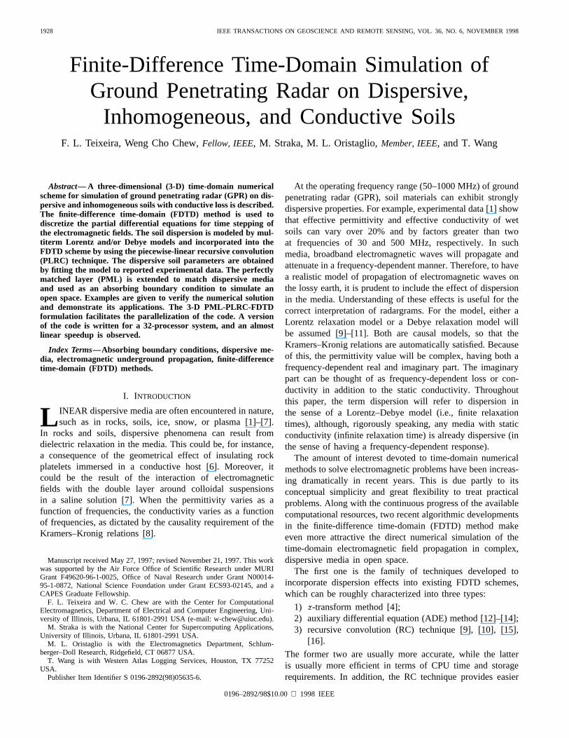
1928 IEEE TRANSACTIONS ON GEOSCIENCE AND REMOTE SENSING, VOL. 36, NO. 6, NOVEMBER 1998

Finite-Difference Time-Domain Simulation ofGround Penetrating Radar on Dispersive,

Inhomogeneous, and Conductive SoilsF. L. Teixeira, Weng Cho Chew,Fellow, IEEE, M. Straka, M. L. Oristaglio,Member, IEEE, and T. Wang

Abstract—A three-dimensional (3-D) time-domain numericalscheme for simulation of ground penetrating radar (GPR) on dis-persive and inhomogeneous soils with conductive loss is described.The finite-difference time-domain (FDTD) method is used todiscretize the partial differential equations for time stepping ofthe electromagnetic fields. The soil dispersion is modeled by mul-titerm Lorentz and/or Debye models and incorporated into theFDTD scheme by using the piecewise-linear recursive convolution(PLRC) technique. The dispersive soil parameters are obtainedby fitting the model to reported experimental data. The perfectlymatched layer (PML) is extended to match dispersive mediaand used as an absorbing boundary condition to simulate anopen space. Examples are given to verify the numerical solutionand demonstrate its applications. The 3-D PML-PLRC-FDTDformulation facilitates the parallelization of the code. A versionof the code is written for a 32-processor system, and an almostlinear speedup is observed.

Index Terms—Absorbing boundary conditions, dispersive me-dia, electromagnetic underground propagation, finite-differencetime-domain (FDTD) methods.

I. INTRODUCTION

L INEAR dispersive media are often encountered in nature,such as in rocks, soils, ice, snow, or plasma [1]–[7].

In rocks and soils, dispersive phenomena can result fromdielectric relaxation in the media. This could be, for instance,a consequence of the geometrical effect of insulating rockplatelets immersed in a conductive host [6]. Moreover, itcould be the result of the interaction of electromagneticfields with the double layer around colloidal suspensionsin a saline solution [7]. When the permittivity varies as afunction of frequencies, the conductivity varies as a functionof frequencies, as dictated by the causality requirement of theKramers–Kronig relations [8].

Manuscript received May 27, 1997; revised November 21, 1997. This workwas supported by the Air Force Office of Scientific Research under MURIGrant F49620-96-1-0025, Office of Naval Research under Grant N00014-95-1-0872, National Science Foundation under Grant ECS93-02145, and aCAPES Graduate Fellowship.

F. L. Teixeira and W. C. Chew are with the Center for ComputationalElectromagnetics, Department of Electrical and Computer Engineering, Uni-versity of Illinois, Urbana, IL 61801-2991 USA (e-mail: w-chew@uiuc.edu).

M. Straka is with the National Center for Supercomputing Applications,University of Illinois, Urbana, IL 61801-2991 USA.

M. L. Oristaglio is with the Electromagnetics Department, Schlum-berger–Doll Research, Ridgefield, CT 06877 USA.

T. Wang is with Western Atlas Logging Services, Houston, TX 77252USA.

Publisher Item Identifier S 0196-2892(98)05635-6.

At the operating frequency range (50–1000 MHz) of groundpenetrating radar (GPR), soil materials can exhibit stronglydispersive properties. For example, experimental data [1] showthat effective permittivity and effective conductivity of wetsoils can vary over 20% and by factors greater than twoat frequencies of 30 and 500 MHz, respectively. In suchmedia, broadband electromagnetic waves will propagate andattenuate in a frequency-dependent manner. Therefore, to havea realistic model of propagation of electromagnetic waves onthe lossy earth, it is prudent to include the effect of dispersionin the media. Understanding of these effects is useful for thecorrect interpretation of radargrams. For the model, either aLorentz relaxation model or a Debye relaxation model willbe assumed [9]–[11]. Both are causal models, so that theKramers–Kronig relations are automatically satisfied. Becauseof this, the permittivity value will be complex, having both afrequency-dependent real and imaginary part. The imaginarypart can be thought of as frequency-dependent loss or con-ductivity in addition to the static conductivity. Throughoutthis paper, the term dispersion will refer to dispersion inthe sense of a Lorentz–Debye model (i.e., finite relaxationtimes), although, rigorously speaking, any media with staticconductivity (infinite relaxation time) is already dispersive (inthe sense of having a frequency-dependent response).

The amount of interest devoted to time-domain numericalmethods to solve electromagnetic problems have been increas-ing dramatically in recent years. This is due partly to itsconceptual simplicity and great flexibility to treat practicalproblems. Along with the continuous progress of the availablecomputational resources, two recent algorithmic developmentsin the finite-difference time-domain (FDTD) method makeeven more attractive the direct numerical simulation of thetime-domain electromagnetic field propagation in complex,dispersive media in open space.

The first one is the family of techniques developed toincorporate dispersion effects into existing FDTD schemes,which can be roughly characterized into three types:

1) -transform method [4];2) auxiliary differential equation (ADE) method [12]–[14];3) recursive convolution (RC) technique [9], [10], [15],

[16].

The former two are usually more accurate, while the latteris usually more efficient in terms of CPU time and storagerequirements. In addition, the RC technique provides easier

0196–2892/98$10.00 1998 IEEE

TEIXEIRA et al.: SIMULATION OF GPR ON SOILS 1929

treatment for the case of dispersive media with multiple polesin the susceptibility function, an important aspect for treatmentof more complex media. A recently proposed extension ofthe RC technique [and demonstrated for one-dimensional(1-D) problems] is the piecewise-linear recursive convolution(PLRC) [17], which has an accuracy similar to the otherapproaches and retains the advantages of the RC approach.In this paper, we apply the PLRC technique to a three-dimensional (3-D) simulation. Since the PLRC is alocalmodification on the update equations, there is no conceptualdifference between the PLRC as applied to 1-D simulationsand the PLRC for two-dimensional (2-D) and 3-D simulations.

The second recent development in the FDTD method con-sisted in the introduction of the perfectly matched layer(PML) as an absorbing boundary condition (ABC) [18]–[20]to simulate open space on a finite computational grid. Apartfrom its numerical efficiency, one of the major advantages ofthe PML over the previously proposed ABC [21]–[24] is thatits absorption properties hold independently of the frequencyof the incident wave. Also, most previously proposed ABC’sare not suited for dispersive media because they requireknowledge of the wave velocity near the grid boundary, aquantity that is not well defined in the time domain fordispersive media. Another advantage of the PML is that itpreserves the nearest-neighbor-interaction characteristic of theFDTD method, making it ideally suited for implementation ona single-instruction multiple-data (SIMD) massively parallelcomputer.

However, the PML, as originally devised, also appliesonly to nondispersive media. In order to apply it for GPRsimulations in dispersive media, it is necessary to extendthe PML to handle dispersive media. Very recently, the firstextensions of the PML to dispersive media for a 1-D PML(single planar boundary) were considered in [25] and [26].The extension proposed in [25] was based on the anisotropicPML formulation [27]. A single-term Lorentz media wasconsidered. The dispersive modeling was implemented usingthe ADE approach, making it difficult to extend for mediawith multiterm dispersion models. On the other hand, theextension in [26] was based on a modification of the originalPML approach of Berenger [18], and, as a result, a differentset of frequency-dependent constitutive parameters had to becarefully derived for the PML media to achieve the perfectmatching condition for the dispersive media at all frequencies.Moreover, this extension is dependent on the specific choiceof dispersion model being used (i.e., Lorentz, Drude, Debye,etc.). Also, in [25] and [26], no indication is given on how totreat, using these approaches, the PML corner regions of thecomputational domain, which play a pivotal role in 2-D and3-D simulations.

In contrast, this paper extends the PML to 3-D dispersivemedia by using the complex coordinate stretching approach[20]. Some advantages of using this approach for dispersivemedia can be listed as follows.

1) There is no need to derive constitutive parameters forthe PML medium. This is because, to achieve the perfectmatching condition in this approach, thesameconstitu-tive parameters can be assumedeverywhere(i.e., both

in the physical and PML regions). The PML region isthen simply defined as the region where the complexstretching is enforced.

2) Treatment of corner regions poses no special difficultysince it just corresponds to regions where simultaneousstretching in different directions are enforced. Therefore,2-D and 3-D simulations can be easily treated. To illus-trate this point, all of the equations in the formulationwill be presented for a situation in which there aresimultaneous stretching on all three directions. Caseswith stretching only along some of the coordinates arejust special cases of the equations presented with thecomplex stretching variables on the remaining coordi-nates set equal to unity.

3) It is particularly suited to be combined with the disper-sion modeling techniques based on recursive convolu-tion, such as the PLRC, thus providing easier treatmentof multiterm Lorentz or Debye models.

4) Since the same set of equations is used both inside thephysical and PML regions (the physical region can beconsidered as a special case of a PML region with allcomplex stretching variables equal to unity), an easierparallelization of the code is made possible.

Some previous numerical simulations of GPR using theFDTD method or the closely related transmission-line matrix(TLM) method were considered in [28]–[38]. In particular, therecent 3-D analysis of [35] already included dispersion effectsand a detailed modeling of the receiving and transmittingantennas. However, no ABC was used to truncate the compu-tational domain, so that unwanted reflections due to the gridtermination were presented and had to be eliminated throughwindowing the results in time (which required larger simula-tion domains) combined with a subtracting procedure (whichrequired multiple simulations). Also, the dispersion modelused was a simplified one in the sense that a low-frequencyapproximation was used for the single-term Debye model.

In this paper, the extension of the 3-D PML to dispersivemedia outlined above is combined with the PLRC techniquein a unified numerical scheme to further enhance the accuracyof FDTD simulations of electromagnetic wave propagation forGPR applications. Multiterm second-order Lorentz and first-order Debye dispersion models for the soils are explicitlytreated in this scheme. In the time-domain, the resultant 3-DPML-PLRC-FDTD scheme is implemented based on a splitform of Maxwell’s equations. The dispersive soils modelparameters are obtained by curve-fitting reported experimentaldata. Examples including the response of buried objects ondispersive soils with conductive loss are given to verifythe numerical solutions and demonstrate its applications. Toillustrate the suitability of the proposed numerical schemeto parallel simulations, a parallelized version of the code iswritten for a 32-processor system and is shown to have analmost linear speedup.

II. PML-FDTD FORMULATION OF DISPERSIVEMEDIA

The PML ABC can be related to a complex coordinatestretching in the frequency domain [20]. This complex stretch-

1930 IEEE TRANSACTIONS ON GEOSCIENCE AND REMOTE SENSING, VOL. 36, NO. 6, NOVEMBER 1998

ing modifies the Maxwell’s equations by adding additionaldegrees of freedom to achieve the reflectionless absorptionof the waves inside the PML region. In the time-domain,the electromagnetic fields components need to be split intosubcomponents. This splitting generally doubles the memoryrequirements of an FDTD simulation. When conductive loss isadded, this further increases the memory requirements becauseof an added conductivity term in the PML equation. It will beshown that the inclusion of dispersion further increases thememory requirements.

The modified Maxwell’s equations in the complex coordi-nate stretching PML formulation are [20]

(1)

(2)

for a conductive medium and in the frequency domain (convention). In the above

(3)

where , , and are frequency-dependent complex stretch-ing variables. To facilitate the solution in the time domain, (1)and (2) are usually split as follows:

(4)

(5)

where the same is repeated forand replacing .By letting , where and are

frequency independent, the above becomes

(6)

(7)

The variables and are the added degrees of freedom ofthe modified Maxwell’s equations. The variable in-duces the reflectionless absorption of propagating modes insidethe PML, and the variable enhances the attenuationrate of evanescent waves, if they exist. In the physical domain,

and , so that the above equations reduce to theusual Maxwell’s equations. Transforming the above back intothe time domain, we obtain

(8)

(9)

In the above, for a dispersive medium, we letwhile

(10)

An -species Lorentzian dispersive medium is characterizedby a frequency-dependent relative permittivity function givenby

(11)

where is the medium susceptibility, is the resonantfrequency for the th species, is the correspondent damp-ing factor, and , are the static and infinite frequencypermittivities, respectively. In the time domain, a complexsusceptibility function [10] can be defined

(12)

where

(13a)

(13b)

and

(13c)

so that the time-domain susceptibility function isand . For a

Debye model, the frequency-dependent permittivity functionis written as

(14)

In this formula, is the pole amplitude and is therelaxation time for the th species. Note that the complexsusceptibility function for the Debye relaxation model canbe considered as a special case of (12) when and

. Hence, the expression (12) applies tobothmodels through a proper choice of parameters.

The electric flux is related to the electric field via

(15)

Using (12) in (15), we have, for both models

(16)

When and using a piecewise-linear approximation forthe electric field in the time-discretization scheme, such that

(17)

(16) then becomes

(18)

TEIXEIRA et al.: SIMULATION OF GPR ON SOILS 1931

where

(19)In the above, and are constants, which depend on theparameters of the particular model, given by

(20a)

(20b)

can be calculated recursively through

(21)where .

The above equations allow the computation ofgivenas the input. However, we would like to computegivenas the input in an FDTD scheme, as we shall see later. To thisend, we substitute (21) into (18) to obtain

(22)

or that

(23)

where

(24a)

(24b)

(24c)

depends only on .

III. T IME-STEPPING SCHEME

We need to devise a time-stepping scheme for (8) and (9).The space discretization is done according to the usual Yeestaggered-grid with central differencing scheme [39] so that

we will not discuss it here. The time discretization for themis as follows:

(25)

(26)

where . Equation (25) can be easily rear-ranged for time stepping

(27)

(28)

However, the left-hand side of (28) depends on both and, making it unsuitable for time stepping. To remove this

problem, we substitute (23) into the left-hand side of (28) sothat we have

(29)

The above equation is now suitable for time stepping andupdating . After is updated and henceis updated, it is used in (29) to update . On the right-hand side of (29), the other pertinent quantities are updatedas follows:

(30a)

(30b)

(30c)

(30d)

The above scheme is repeated forreplaced with and. Hence, (27), (29), and (30) constitute the complete

PML-PLRC-FDTD updating scheme for the electromagneticfields. Note that, due to the use of a backward Euler’s method(forward difference in time) in the time-update scheme of (25)and (26) and the neglect of in (26) [which differs from

by ], the above scheme is only first-order accuratein time. This is chosen mainly due to its simplicity and tothe fact that less arithmetic operations are required at eachtime step. Another advantage is that this is a conditionallystable scheme in the diffusion regime. If needed, a second-order accurate scheme can be easily derived through parallellines, by employing, for example, a trapezoidal rule time-update scheme (leapfrog scheme). However, this last scheme,when combined with the central-differencing scheme in spacecharacteristic of the FDTD method, is not stable anymore inthe diffusion regime [8].

1932 IEEE TRANSACTIONS ON GEOSCIENCE AND REMOTE SENSING, VOL. 36, NO. 6, NOVEMBER 1998

Storage is required for , , , ,, , and since each has two

vector components, we need to store valueswhere is the number of simulation nodes and is thenumber of species in the relaxation model. The added storagecost of simulating a PML dispersive medium is 6 , whilethe added cost of a PML conductive medium is to store

, which is 6 . A nondispersive, nonconductive PMLmedium will require 12 storage as opposed to the 6needed in the plain Yee scheme. Although (29) and (30)seem to suggest the need to store the electric field at twosuccessive time steps, this can be avoided in the numericalalgorithm by storing, at each time step, the electric fieldat the previous time step in a temporary variable [17].Therefore, the use of a piecewise-linear approximation (17)in the constitutive relation does not incuradditional storage requirements in comparison to a piecewise-constant approximation. It should be pointed out that arbitrarysusceptibility functions can, in principle, be modeled as asum of Lorentz and/or Debye terms. This can be done, e.g.,by first evaluating the dielectric permittivity and the effectiveconductivity for various frequencies and then curve fittingthe result by a meromorphic function expanded as a partialfraction expansion [40] with (possibly) single poles (Debyeterms), complex conjugate poles (Lorentz terms), and a poleat (static conductivity term), plus a constant termstanding for the permittivity at infinite frequency. This willbe illustrated in the next section.

IV. NUMERICAL SIMULATION RESULTS

An FDTD code has been written using the formulation ofprevious sections. A PML medium is assumed everywhere sothat the code can be easily parallelized, allowing operation inthe SIMD (single-instruction multiple-data) mode.

To first validate the formulation, the results from the FDTDsimulation for a homogeneous dispersive half-space problemwith conductive loss are compared against a pseudoanalyticalsolution. The pseudoanalytical solution is obtained by first nu-merically integrating the frequency-domain Sommerfeld inte-grals of the half-space problem for many excitation frequencies[8]. The result is then multiplied by the spectrum of the sourcepulse and, subsequently, inverse Fourier transformed to yieldthe time-domain solution. Fig. 1 compares the results for theFDTD simulation using both the PML-RC (piecewise-constantelectric field) approach and the PML-PLRC (piecewise-linearelectric field) in a dispersive half-space against this pseudo-analytical solution. The half-space dispersion parameters areobtained by fitting a two-species ( ) Debye model [33] tothe experimental data reported by Hipp [1] for the Puerto Ricotype of claim loams, as given in Table I. The experimental andmodel data are plotted in Figs. 2 and 3. As seen, the model datafit the experimental data reasonably well. The specific curvetaken for the comparison of Fig. 1 is the 5% moisture contentcase with the model parameters given in Table I. The PMLfor this example is set with ten layers with a quadratic taper[18]–[20]. The source pulse is the first derivative of a slightlydifferent version of the Blackmann–Harris pulse [41] so that

Fig. 1. Sommerfeld solution (solid line) versus PML-FDTD solution usingRC (dotted line) and PLRC (dashed line) for an infinitesimal vertical electricdipole radiating on top of a dispersive half-space modeled by a two-speciesDebye model. The PLRC approach presents a better agreement against thepseudoanalytical Sommerfeld solution.

TABLE IDEBYE-MODEL PARAMETERS OF THEPUERTO RICO-TYPE CLAY LOAMS

Fig. 2. Dielectric permittivity of the Puerto Rico type of clay loams versusfrequency [1]. The solid lines indicate the experimental data, and the dashedlines indicate the model-fitting data. The numbers indicate the content ofmoisture.

the pulse vanishes completely after a time period .The central frequency is at MHz. Note that with thisfrequency of operation (typical of GPR applications) and withthe relaxation times presented in Table I, we have ,so that it is not possible to use a low-frequency approximationfor the Debye model. The half-space occupies 60% of thevertical height of the cubic simulation region. The simulationis done with a grid with

TEIXEIRA et al.: SIMULATION OF GPR ON SOILS 1933

Fig. 3. Same as Fig. 2, except for the effective conductivity.

a space discretization size cm and a time stepps. Assuming that the origin is at a corner of

the cube, the source is a vertical electric dipole (-directed)located at and the -componentof the electric field is sampled at .The field is deliberately sampled inside the half-space so thatit is more sensitive to its dispersive properties.

The results show an agreement between the formulations. Inparticular, this figure illustrates the improvement in accuracyby using the PLRC against the RC scheme. Also, no noticeablereflection due to the grid termination is present.

In what follows, a series of examples of the numericalsimulation of the GPR response of a pipeline buried on thePuerto Rico type of claim loams with different moisturecontents will be presented. The pipe is either metallic orplastic, buried 2 m deep, and has a diameter of 6 in. Boththe transmitter and receiver dipoles are parallel to the metalpipe. Note that this is a 2.5 problem [30]; i.e., there isinvariance of the geometry in one direction (meaning theinhomogeneity is 2-D), but the field distribution is 3-D due tothe source configuration. In this kind of problems, we can takeadvantage of thespatialinvariance in one dimension and applya Fourier transformation in that direction to eliminate one ofthe spatial derivatives in Maxwell’s equations. This allows aproperly modified 2-D FDTD scheme to solve the full-wave3-D problem [30], [33]. In our simulations, however, it will besolved using the full 3-D code. The simulation is done with a

grid. The space discretizationis m, and the time step is ps. Theair–ground interface is located at . The pipe pointsin the direction and is centered at . Thetransmitter and receiver are located just above the ground. Thetransmitter is fixed at , and the re-ceiver moves in a straight line in thedirection (perpendicularto the pipe), from the point to thepoint so that the source-receiveroffset varies from 0.1 to 2.5 m. Fig. 4 illustrates this common-source configuration. Since the emphasis is on the wavepropagation modeling aspect, both the transmitter and receiver

Fig. 4. Common-source configuration of the GPR. See text for details.

considered are just point electric dipoles. For an example on adirect incorporation of a more realistic antenna modeling usingthe FDTD scheme, refer to the approaches described in [34]and [35], where bowtie antennas are considered. Alternatively,we can also incorporate aperture antennas directly in the modelby using an array of equivalent point dipoles positioned on theantenna aperture, with the strength parameters (weights) ofeach dipole being determined by a calibration procedure [38].

For these examples, the source pulse used is again a deriva-tive of the Blackmann–Harris pulse centered at 200 MHz. ThePML absorbing boundary condition is set with ten PML with aquadratic taper increasing from the physical domain interfacetoward the grid ends.

Fig. 5(a)–(c) compare the numerical simulation, with andwithout dispersion included, of the common-source radartraces for a metal pipe in soils with 2.5, 5, and10% of moisture. The model parameters for the simulationwith dispersion are taken from Table I, and the constitutiveparameters of the simulation without dispersion are takenfrom Figs. 2 and 3 at the center frequency of 200 MHz. Thesimulated traces are normalized to the maximum field valueat the receiver for each receiver position. From Fig. 5 (a)–(c),we first note that, for increased moisture content, the simulatedecho appears later and is subjected to a stronger attenuation,in agreement with Figs. 2 and 3, where it is seen that boththe effective conductivity and the effective dielectric constantincreases with increasing moisture contents.

To better illustrate the effects of the dispersion on thereflected pulse, Fig. 6(a)–(c) single out a view of the simulatedtraces obtained with the simulation with and without dispersion[same cases of Fig. 5(a)–(c)] at a specific offset of 2.0 m.Despite the insignificant differences on the first arrival times, itis seen that the dispersion may distort the pulse shape againstthe nondispersive simulation. For example, in Fig. 6(a), thereflected pulse in the presence of dispersion becomes lesssymmetric with respect to its main lobe than in the simulationwithout dispersion.

1934 IEEE TRANSACTIONS ON GEOSCIENCE AND REMOTE SENSING, VOL. 36, NO. 6, NOVEMBER 1998

(a)

(b)

(c)

Fig. 5. Simulation of the radar traces (common-source configuration), cal-culated with and without dispersion, of a metal pipe on a soil with: (a) 2.5%,(b) 5.0%, and (c) 10.0% of moisture. The dielectric constant and conductivityfor the simulation without dispersion are picked from Figs. 2 and 3 at thecentral frequency of 200 MHz. Increased moisture contents tend to slow andincrease the attenuation of the reflected pulse from the pipe.

Fig. 7 presents the simulated radar traces of a plastic pipeon a soil with 2.5% of moisture, with

dispersion modeling included and model parameters takenfrom Table I, against a simulation without dispersion withconstitutive parameters taken from Figs. 2 and 3 at 200 MHz.

(a)

(b)

(c)

Fig. 6. Radar trace simulation taken from Fig. 5(a)–(c) at an offset of 2.0 m,calculated with and without dispersion, in soils with: (a) 2.5%, (b) 5.0%, and(c) 10.0% of moisture.

TEIXEIRA et al.: SIMULATION OF GPR ON SOILS 1935

Fig. 7. Simulation of the radar trace (common-source configuration), calcu-lated with and without dispersion, of a plastic pipe on a soil with 2.5% ofmoisture. The dielectric constant and conductivity for the simulation withoutdispersion are picked from Figs. 2 and 3 at the central frequency of 200 MHz.Due to the less-reflective nature of the plastic material, the reflected trace isless visible.

Fig. 8. Radar trace simulation taken from Fig. 7 at an offset of 2.0 m,calculated with and without dispersion.

The geometry is the same as in the metallic pipe example.Due to the less-reflective nature of the plastic material, thereflected trace is now much weaker.

Fig. 8 singles out the simulated response of the plasticpipe response taken at an offset of 2 m for the dispersiveand nondispersive cases. The difference between the reflectedpulses for the dispersive and nondispersive cases is lessapparent than in the metallic case.

It should be emphasized that the above observations aremade based on the specific choice of the nondispersive soil pa-rameters and on the kind of soil and buried object considered.The details may vary for different choices of the parame-ters and soils. It is not the intention here to exhaust thesescenarios.

A version of the code has been parallelized to run on a32-processor SGI R10000. Fig. 9 shows the speed of the code(running a two-species dispersive model) for 1000 time stepsas a function of the number of active processors. The speed

Fig. 9. Speed of the code as a function of the number of processors on a32-processor SGI R10000 machine. The problem size is 50� 50� 50. Analmost linear speedup is observed up to 12 active processors, but performancedeteriorates for this problem size as the number of processors further increases.

is defined as the inverse of the real CPU time on an emptymachine (single-user). The problem size is 5050 50. Analmost linear speedup to 12 processors is observed. For thisproblem size, not much more speedup past 12–15 processorsis expected due to the communication overhead and load im-balance between the processors. However, for larger problemssizes, increased speedup can be expected with a larger numberof active processors.

V. CONCLUSIONS

A 3-D FDTD numerical simulation of the GPR responseon dispersive media with conductive loss is described. Thedispersive effect is modeled by a multiterm Lorentz and/orDebye model. The electric field convolution is implementedby the PLRC. The PML is extended to match dispersivemedia and used as an absorbing boundary condition. By aproper choice of the parameters, the media can exhibit thedispersive effects observed in some soils and rocks. The 3-DPML-PLRC-FDTD numerical simulations with buried metaland plastic pipes buried on dispersive soils show that thereflected pulse (and, hence, the GPR response) can be affectedby dispersive effects. In addition to its inherent numericalefficacy, the use of the PML allows the easy parallelizationof the code. However, the use of the PML and dispersivemedia modeling comes with the added cost of more memoryrequirements and computational time. A version of the codewas paralleled and shown to have an almost linear speedup.

ACKNOWLEDGMENT

The authors acknowledge the reviewers for their usefulsuggestions regarding this paper. Part of the computer timewas provided by the National Center for SupercomputingApplications, University of Illinois.

REFERENCES

[1] J. E. Hipp, “Soil electromagnetic parameters as functions of frequency,soil density, and soil moisture,”Proc. IEEE,vol. 62, pp. 98–103, Jan.1974.

1936 IEEE TRANSACTIONS ON GEOSCIENCE AND REMOTE SENSING, VOL. 36, NO. 6, NOVEMBER 1998

[2] W. D. Hurt, “Multiterm Debye dispersion relations for permittivity ofmuscle,” IEEE Trans. Biomed. Eng.,vol. 32, pp. 60–64, Jan. 1985.

[3] D. Sullivan, “A frequency-dependent FDTD method for biological ap-plications,” IEEE Trans. Microwave Theory Tech.,vol. 40, pp. 532–539,Apr. 1992.

[4] , “Frequency-dependent FDTD methods usingz transforms,”IEEE Trans. Antennas Propagat.,vol. 40, pp. 1223–1230, Nov.1992.

[5] O. P. Gandhi, B. Q. Gao, and J. Y. Chen, “A frequency-dependent finite-difference time-domain formulation for general dispersive media,”IEEETrans. Microwave Theory Tech.,vol. 41, pp. 658–664, May 1993.

[6] P. N. Sen and W. C. Chew, “The frequency dependent dielectric andconductivity response of sedimentary rocks,”J. Microw. Power,vol.18, no. 1, p. 95, 1983.

[7] W. C. Chew and P. N. Sen, “Dielectric enhancement due to electrochem-ical double layer: Thin double layer approximation,”J. Chem. Phys.,vol. 77, no. 9, p. 4683, 1982.

[8] W. C. Chew,Waves and Fields in Inhomogeneous Media.New York:Van Nostrand Reinhold, 1990, reprinted by IEEE Press, 1995, ch. 4.

[9] R. Luebbers, F. P. Hunsgerger, K. S. Katz, R. B. Standler, and M.Schneider, “A frequency-dependent finite-difference time-domain for-mulation for dispersive materials,”IEEE Trans. Electromagn. Compat.,vol. 32, pp. 222–227, Feb. 1990.

[10] R. Luebbers and F. P. Hunsberger, “FDTD forN -th order dispersivemedia,” IEEE Trans. Antennas Propagat.,vol. 40, pp. 1297–1301, Dec.1992.

[11] C. M. Rappaport and W. H. Weedon, “Computational issues in groundpenetrating radar,” Center Electromagn. Res., Northeastern Univ.,Boston, MA, Unpublished Rep., 1994.

[12] T. Kashiva, Y. Ohtomo, and I. Fukai, “A finite-difference time-domainformulation for transient propagation in dispersive media associated withCole–Cole’s circular arc law,”Microwave. Opt. Technol. Lett.,vol. 3,no. 12, pp. 416–419, 1990.

[13] R. M. Joseph, S. C. Hagness, and A. Taflove, “Direct time integrationof Maxwell’s equations in linear dispersive media with absorption forscattering and propagation of femtosecond electromagnetic pulses,”Opt.Lett., vol. 16, pp. 1412–1414, 1991.

[14] O. P. Gandhi, B.-Q. Gao, and J.-Y. Chen, “A frequency-dependentfinite-difference time-domain formulation for general dispersive media,”IEEE Trans. Microwave Theory Tech.,vol. 41, pp. 658–664, May1993.

[15] M. D. Bui, S. S. Stuchly, and G. I. Coustache, “Propagation of transientsin dispersive dielectric media,”IEEE Trans. Microwave Theory Tech.,vol. 39, pp. 1165–1171, Oct. 1991.

[16] R. J. Hawkins and J. S. Kallman, “Linear electronic dispersion and finite-difference time-domain calculations: A simple approach,”J. LightwaveTechnol.,vol. 11, pp. 1872–1874, 1993.

[17] D. F. Kelley and R. J. Luebbers, “Piecewise linear recursive convolutionfor dispersive media using FDTD,”IEEE Trans. Antennas Propagat.,vol. 44, pp. 792–797, June 1996.

[18] J. P. Berenger, “A perfectly matched layer for the absorption ofelectromagnetic waves,”J. Comput. Phys.,vol. 114, pp. 185–200,1994.

[19] D. S. Katz, E. T. Thiele, and A. Taflove, “Validation and extension tothree dimensions of the Berenger PML absorbing boundary conditionfor FD-TD meshes,”IEEE Microwave Guided Wave Lett.,vol. 4, pp.268–270, Feb. 1994.

[20] W. C. Chew and W. H. Weedon, “A 3D perfectly matched medium frommodified Maxwell’s equations with stretched coordinates,”MicrowaveOpt. Technol. Lett.,vol. 7, pp. 599–604, 1994.

[21] A. Bayliss and E. Turkel, “Radiation boundary conditions for wave-likeequations,”Commun. Pure Appl. Math.,vol. 33, pp. 707–725, 1980.

[22] G. Mur, “Absorbing boundary conditions for the finite-difference ap-proximation of the time domain electromagnetic field equations,”IEEETrans. Electromagn. Compat.,vol. EMC-23, pp. 377–382, May 1981.

[23] Z. P. Liao, H. L. Wong, B. P. Yang, and Y. F. Yuan, “A transmittingboundary for transient wave analysis,”Scientia Sinica-A,vol. 27-A, pp.1063–1076, 1984.

[24] K. K. Mei and J. Fang, “Superabsorption—A method to improveabsorbing boundary conditions,”IEEE Trans. Antennas Propagat.,vol.40, pp. 1001–1010, Sept. 1992.

[25] S. D. Gedney, “An anisotropic PML absorbing media for the FDTDsimulation of fields in lossy and dispersive media,”Electromagnetics,vol. 16, pp. 399–415, 1996.

[26] T. Uno, Y. He, and S. Adachi, “Perfectly matched layer absorbingboundary condition for dispersive medium,”IEEE Microwave GuidedWave Lett.,vol. 7, pp. 264–266, Sept. 1997.

[27] Z. S. Sacks, D. M. Kingsland, R. Lee, and J.-F. Lee, “A perfectly

matched anisotropic absorber for use as an absorbing boundary con-dition,” IEEE Trans. Antennas Propagat.,vol. 43, pp. 1460–1463, Dec.1995.

[28] C. Liu and L. C. Chen, “Numerical simulation of subsurface radar fordetecting buried pipes,”IEEE Trans. Geosci. Remote Sensing,vol. 29,pp. 795–798, July 1991.

[29] M. Moghaddam, W. C. Chew, B. Anderson, E. Yannakis, and Q. H. Liu,“Computation of transient electromagnetic waves in inhomogeneousmedia,” Radio Sci.,vol. 26., no. 1, pp. 265–273, 1991.

[30] M. Moghaddam, E. J. Yannakakis, W. C. Chew, and C. Randall,“Modeling of the subsurface interface radar,”J. Electromagn. WavesApplicat., vol. 5, pp. 17–39, 1991.

[31] Y. He, T. Uno, S. Adachi, and T. Mashiko, “Two-dimensional activeimaging of conducting objects buried on a dielectric half-space,”IEICETrans. Commun.,vol. E76-B, no. 12, pp. 1546–1551, 1993.

[32] K. Demarest, R. Plumb, and Z. Huang, “The performance of FDTDabsorbing boundary conditions for buried scatterers,” inProc. URSIRadio Sci. Mtg.,1994, p. 169.

[33] T. Wang, M. L. Oristaglio, and W. C. Chew, “Finite-difference simula-tion of ground penetrating radar in dispersive soils,” Schlumberger–DollResearch, Ridgefield, CT, SDR-EMG Res. Note, Dec. 1995.

[34] B. J. Hook, “FDTD modeling of ground-penetrating radar antennas,” inProc. 11th Annu. Rev. Prog. Appl. Comp. Electromag.,Monterey, CA,1995, pp. 740–747.

[35] J. M. Bourgeois and G. S. Smith, “A fully three-dimensional simulationof a ground-penetrating radar: FDTD theory compared with experi-ment,” IEEE Trans. Geosci. Remote Sensing,vol. 34, pp. 36–44, Jan.1996.

[36] J. Calhoun, “A finite difference time domain (FDTD) simulation ofelectromagnetic wave propagation and scattering in a partially conduct-ing layered earth,” inProc. 1997 IGARSS—Int. Geosci. Remote SensingSymp.,pp. 922–924.

[37] G. A. Newman and D. L. Alumbaugh, “3D Electromagnetic modelingusing staggered finite differences,” inProc. 1997 IGARSS—Int. Geosci.Remote Sensing Symp.,pp. 929–931.

[38] S. Agosti, G. G. Gentili, and U. Spagnolini, “Electromagnetic inversionof monostatic GPR: Application to pavement profiling,” inProc. 1997Int. Conf. Electromag. Adv. Applicat. (ICEAA’97),pp. 491–494.

[39] K. S. Yee, “Numerical solution of initial boundary value problemsinvolving Maxwell’s equation in isotropic media,”IEEE Trans. AntennasPropagat.,vol. 14, pp. 302–307, Feb. 1966.

[40] E. C. Levy, “Complex-curve fitting,”IRE Trans. Automat. Control,pp.37–43, May 1959.

[41] F. J. Harris, “On the use of windows for harmonic analysis with thediscrete Fourier transform,”Proc. IEEE,vol. 66, pp. 51–83, Jan. 1978.

F. L. Teixeira received the M.S.E.E. degree fromthe Pontifical Catholic University, Rio de Janeiro,Brazil, in 1995. He is currently pursuing the Ph.D.degree in electrical engineering at the University ofIllinois at Urbana-Champaign.

He was a Technical Officer with the Brazil-ian Army Research and Development Center (IPD-CTEx) from 1992 to 1994, and from 1994 to 1996,he was a member of the Technical Staff in the Satel-lite Transmission Department, EMBRATEL S.A.(Brazilian Telecom). Since 1996, he has been a

Research Assistant with the Center for Computational Electromagnetics,University of Illinois at Urbana-Champaign. His research interests includewave propagation modeling for communication and sensing applications.

Weng Cho Chew (S’79–M’80–SM’86–F’93), for a photograph and biogra-phy, see p. 748 of the May 1998 issue of this TRANSACTIONS.

TEIXEIRA et al.: SIMULATION OF GPR ON SOILS 1937

M. Straka received the B.S. degree in computerscience and engineering with a minor in astrophysicsfrom the University of Illinois at Urbana-Champaignin 1987.

He has been a Consultant and Applications Pro-grammer with the National Center for Supercom-puting Applications (NCSA), University of Illinoisat Urbana-Champaign, since 1987. His focus is onperformance analysis and optimization techniquesfor large, scalable scientific applications on vec-tor supercomputers and parallel RISC superscalar

processor.

M. L. Oristaglio (M’89) received the B.S. and M.S. degrees in geologyand geophysics from Yale University, New Haven, CT, in 1974, and theM.Sc. degree in geochemistry and the D.Phil. degree in geophysics, bothfrom Oxford University, Oxford, U.K., in 1975 and 1978, respectively.

He was a Postdoctoral Research Associate at the University of Utah,Salt Lake City, and a Gibbs Instructor in Geology and Geophysics at YaleUniversity. He is currently Director of Electromagnetics at Schlumberger–DollResearch, Ridgefield, CT, since 1990. He joined Schlumberger in 1982 asa Research Scientist in the Mechanics-Electrical Department. From 1985to 1987, he was Technical Advisor at Schlumberger Engineering Center,Paris, France. From 1988 to 1990, he was Manager of the WorkstationProducts Department at Schlumberger Austin System Center, Austin, TX.Currently, he is also an Adjunct Professor in the Department of Geologyand Geophysics at the University of Utah and a Visiting Professor in theDepartment of Electrical Engineering, Delft University of Technology, Delft,The Netherlands. His areas of research are forward and inverse problems inacoustics and electromagnetics, chiefly in applied geophysics.

T. Wang received the M.S. degree in geophysics from the Institute ofGeophysics, Chinese Academy of Sciences, Beijing, in 1988 and the Ph.D.degree in geophysics from the University of Utah, Salt Lake City, in 1993.

He was a Postdoctoral Fellow at the University of Utah from 1993 to1994 and a Postdoctoral Fellow at Schlumberger–Doll Research, Ridgefield,CT, from 1994 to 1995. In 1996, he joined Western Atlas Logging Services,Houston, TX. His present research interests include electromagnetic modelingand imaging, signal processing, and borehole geophysics.