High-order non-reflecting boundary conditions for dispersive waves

High-Order Non-ReflectingBoundary Conditionsfor Dispersive Waves

Dan Givoli ∗ Beny Neta †

Department of MathematicsNaval Postgraduate School

1141 Cunningham RoadMonterey, CA 93943, U.S.A.

July 17, 2002

∗Corresponding author. E-mail: [email protected] , Tel.: +1-831-656-2758, Fax: +1-831-656-2355.On leave (till Aug. 2002) from: Department of Aerospace Engineering and Asher Center for Space Research,Technion — Israel Institute of Technology, Haifa 32000, Israel, E-mail: [email protected] ,Tel.: +972-4-8293814, Fax: +972-4-8231848.

†E-mail: [email protected] , Tel.: +1-831-656-2235, Fax: +1-831-656-2355.

High-Order NRBCs for Dispersive Waves 2

Abstract

Problems of linear time-dependent dispersive waves in an unbounded domain are con-sidered. The infinite domain is truncated via an artificial boundary B, and a high-orderNon-Reflecting Boundary Condition (NRBC) is imposed on B. Then the problem is solvedby a Finite Difference scheme in the finite domain bounded by B. The sequence of NRBCsproposed by Higdon is used. However, in contrast to the original low-order implementationof the Higdon conditions, a new scheme is devised which allows the easy use of a Higdon-typeNRBC of any desired order. In addition, a procedure for the automatic choice of the param-eters appearing in the NRBC is proposed. The performance of the scheme is demonstratedvia numerical examples.

Keywords: Waves, High-order, Artificial boundary, Non-reflecting boundary condition,Higdon, Finite Difference.


1. Introduction

In many fields of application involving the propagation of waves, the domain of the problemunder investigation is unbounded (or very large). One of the common methods used for thenumerical solution of such problems [1] is the method of Non-Reflecting Boundary Condi-tions. In this method the original domain is truncated via an artificial boundary B, thusforming a finite computational domain Ω bounded by B. A special boundary condition isimposed on B, in order to complete the statement of the problem (i.e., make the solutionunique) and, most importantly, to ensure that no (or little) spurious wave reflection occursfrom B. Then the problem is solved numerically in Ω.

The boundary condition applied on B is called a Non-Reflecting Boundary Condition(NRBC), although a few other names are often used too [2]. Naturally, the quality of thenumerical solution strongly depends on the properties of the NRBC employed. In the last25 years or so, much research has been done to develop NRBCs that after discretization leadto a scheme which is stable, accurate, efficient and easy to implement. See [3] and [4] forrecent reviews on the subject. Of course, it is difficult to find a single NRBC which is idealin all respects and all cases; this is why the quest for better NRBCs and their associateddiscretization schemes continues.

Some low-order local NRBCs have been proposed in the late 70’s and early 80’s and havebecome well-known, e.g., the Engquist-Majda NRBCs [5] and the Bayliss-Turkel NRBCs [6].The late 80’s and early 90’s have been characterized by the emerging of the exact nonlo-cal Dirichlet-to-Neumann (DtN) NRBC [7, 8] and the Perfectly Matched Layer (PML) [9].More recently, high-order local NRBCs have been introduced. Sequences of increasing-orderNRBCs have been available before (e.g., the Bayliss-Turkel conditions [6] constitute sucha sequence), but they had been regarded as impractical beyond 2nd or 3rd order from theimplementation point of view. Only since the mid 90’s, practical high-order NRBCs havebeen devised.

The first such high-order NRBC has apparently been proposed by Collino [10], for two-dimensional time-dependent waves in rectangular domains. Its construction requires thesolution of the one-dimensional wave equation on B. Grote and Keller [11] developed a high-order converging NRBC for the three-dimensional time-dependent wave equation, basedon spherical harmonic transformations. They extended this NRBC for the case of elasticwaves in [12]. Sofronov [13] has independently published a similar scheme in the Russianliterature. Hagstrom and Hariharan [14] constructed high-order NRBCs for the two- andthree-dimensional time-dependent wave equations based on the analytic series representationfor the outgoing solutions of these equations. It looks simpler than the previous two NRBCs.For time-dependent waves in a two-dimensional wave guide, Guddati and Tassoulas [15] de-vised a high-order NRBC by using rational approximations and recursive continued fractions.Givoli [16] has shown how to derive high-order NRBCs for a general class of wave problems,leading to a symmetric finite element formulation. In [17], this methodology was applied tothe particular case of time-harmonic waves, using optimally localized DtN NRBCs.

Most of the NRBCs mentioned above have been designed for either time-harmonic waves


or for non-dispersive time-dependent waves. The presence of wave dispersion makes the time-dependent problem much more difficult as far as NRBC treatment is concerned. Dispersivemedia appear in various applications. One important example is that of meteorologicalmodels which take into account the earth rotation [18]. Other examples include quantum-mechanics waves, the vibration of structures with rotational rigidity such as beams, platesand shells, and many nonlinear wave problems, with or without linearization. Very recently,Navon et al. [19] developed a PML scheme for the dispersive shallow water equations. In thepresent paper we develop high-order NRBCs for dispersive waves. Naturally, our scheme isjust as applicable to the non-dispersive case, by simply taking the dispersion parameter tobe zero.

Higdon [20] proposed a sequence of NRBCs for the dispersive (Klein-Gordon) wave equa-tion. In fact, these NRBCs were developed originally for non-dispersive waves [21]–[25],but Higdon showed in [20] that they can be applied in the dispersive case too. Indeed, ourscheme is based on Higdon’s NRBCs. However, in contrast to the original low-order for-mulation of these conditions, a new scheme is devised here which allows the easy use of aHigdon-type NRBC of any desired order. In addition, a procedure for the automatic choiceof the parameters appearing in the NRBC is proposed.

Following is the outline of the rest of this paper. In Section 2 we state the problem underinvestigation. We emphasize that the setup taken here, namely that of a semi-infinite waveguide, serves merely as an example, and in fact the proposed approach is general and caneasily be extended to other configurations, such as two-dimensional exterior problems with arectangular artificial boundary. In Section 3 we present the Higdon NRBCs and briefly recalltheir properties. In Section 4 we show how to implement the Higdon NRBCs, using a FiniteDifference (FD) scheme, in a high-order way. Then we show, in Section 5, how the basicFD approximations used in this scheme can be improved if one desires, and in Section 6 wepresent a procedure for the automatic choice of the NRBC parameters. We demonstrate theperformance of the new method via some numerical examples in Section 7. We conclude, inSection 8, with some remarks.

2. Statement of the Problem

We consider the linear inhomogeneous Klein-Gordon equation,

∂2t u− C2

0∇2u+ f 2u = S , (1)

in a two-dimensional uniform semi-infinite channel or wave guide. A Cartesian coordinatesystem (x, y) is introduced such that the wave-guide is parallel to the x direction. The widthof the wave-guide is denoted b. The setup is shown in Fig. 1(a). In (1), u is the unknownwave field, C0 is the given reference wave speed, f is the given dispersion parameter, and S isa given wave source function. The C0 and f are allowed to be functions of location; however,it is assumed that the region where they are not constant is finite (and typically locatednear the west boundary ΓW ). The wave source S is a function of location and time, but it


is assumed to have a local support. Eq. (1) describes, for example, the lateral vibration ofa membrane strip on an elastic foundation, or the acoustic pressure in a dispersive medium(say, a linearized bubbly medium). Also, it can be shown that the linearized shallow waterequations, with a flat bottom and zero initial conditions, reduce to (1), where u is the waterelevation above the reference level [18]. In the geophysical context, f is called the Coriolisparameter and is related to the angular velocity of the earth.

(a)

xΓ

Γ

S

N

W

Γ

y b

(b)

N

S

ΓΓ

Γ

W D

Γ

Ω

E

E

x

y

x=x

b

Figure 1: Setup for the wave-guide problem: (a) the original problem in a semi-infinite waveguide; (b) the computational problem in a finite domain Ω.

On the south and north boundaries ΓS and ΓN we specify the Neumann condition:

∂yu = 0 on ΓS & ΓN . (2)

In acoustics this corresponds to a “hard wall” condition. On the west boundary ΓW weprescribe u using a Dirichlet condition, i.e.,

u(0, y, t) = uW (y, t) on ΓW , (3)

where uW (y, t) is a given function (incoming wave). At x→∞ the solution is known to bebounded and not to include any incoming waves.

To complete the statement of the problem, the initial conditions

u(x, y, 0) = u0 , ∂tu(x, y, 0) = v0 , (4)

are given at time t = 0 in the entire domain. We assume that the functions u0 and v0 havea local support.


We now truncate the semi-infinite domain by introducing an artificial east boundaryB ≡ ΓE, located at x = xE . See Fig. 1(b). This boundary divides the original semi-infinitedomain into two subdomains: an exterior domain D, and a finite computational domain Ωwhich is bounded by ΓW , ΓN , ΓS and ΓE . We choose the location of ΓE such that the entiresupport of S, u0 and v0 and the region of non-uniformity of C0 and f are all contained insideΩ. Thus, on ΓE and in D, the homogeneous counterpart of (1) holds, i.e.,

∂2t u− C2

0∇2u+ f 2u = 0 , (5)

with constant coefficients C0 and f 2, and the medium is initially at rest.To obtain a well-posed problem in the finite domain Ω we need to impose a boundary

condition on ΓE. This must be a Non-Reflecting Boundary Condition (NRBC), so as toprevent spurious reflection of waves. In the next section we discuss the choice of this NRBC.

3. Higdon’s NRBCs

On the artificial boundary ΓE we use one of the Higdon NRBCs [20]. These NRBCs werepresented and analyzed in a sequence of papers [21]–[25] for non-dispersive acoustic andelastic waves, and were extended in [20] for the dispersive case. The Higdon NRBC of orderJ is

HJ :

J∏

j=1

(∂t + Cj∂x)

u = 0 on ΓE . (6)

Here, the Cj are parameters which have to be chosen and which signify phase speeds in thex-direction. The main advantages of the Higdon conditions are as follows:

• The Higdon NRBCs are very general, namely they apply to a variety of wave problems,in one, two and three dimensions and in various configurations. Moreover, they can beused, without any difficulty, for dispersive wave problems and for problems with layers.Most other available NRBCs are either designed for non-dispersive homogeneous media(as in acoustics and electromagnetics) or are inherently of low order (as in meteorologyand oceanography).

• The Higdon NRBCs constitute a sequence of conditions of increasing order. This, andthe fact that no asymptotic approximation is involved in their construction, enables onein principle (leaving implementational issues aside for the moment) to obtain solutionswith unlimited accuracy.

• For certain choices of the parameters, the Higdon NRBCs are equivalent to NRBCsthat are derived from rational approximation of the dispersion relation (the Engquist-Majda conditions [5] being the most well-known example). This has been proved byHigdon in [20, 21]. More precisely, Higdon’s theorem states that if a NRBC is basedon a symmetric rational approximation to the dispersion relation corresponding to


outgoing waves, then it is either (a) equivalent to (6) for a suitable choice of J andthe parameters Cj, or (b) unstable, or (c) not optimal. Lack of optimality meanshere that the coefficients in the NRBC can be modified so as to reduce the amount ofthe spurious reflection. Thus, the Higdon NRBCs can be viewed as generalization ofrational-approximation NRBCs.

The scheme developed here is different than the original Higdon scheme [20] in the fol-lowing ways:

(a) The discrete Higdon conditions were developed in the literature up to third order only,because of their algebraic complexity which increases rapidly with the order. Herewe show how to easily implement these conditions to an arbitrarily high order. Thescheme is coded once and for all for any order; the order of the scheme is simply aninput parameter.

(b) The Higdon NRBCs involve some parameters which must be chosen. Higdon [20] dis-cusses some general guidelines for their manual a-priori choice by the user. We shallshow how these parameters can be chosen automatically.

(c) We shall show how to improve the discretization of the basic operators involved in theHigdon NRBCs, by using more accurate FD stencils, and how to incorporate theseimproved discretizations in the new scheme.

We now make a few remarks recalling the properties of the Higdon NRBCs.

1. The boundary condition (6) is exact for all waves that propagate with an x-directionphase speed equal to either of C1, . . . , CJ . To see this, consider a wave which satisfiesthe wave equation (5) with constant C0 and f . Such a wave has the form

u = A cosnπy

bcos(kx− ωt+ ψ) , (7)

where

ω2 = C20

(k2 +

n2π2

b2

)+ f 2 , n = 0, 1, 2, . . . (8)

Also, let

Cx =ω

k, (9)

which is the x-direction phase velocity. In (7)–(9), A is the wave amplitude, ψ is itsphase, k is the x-component wave number, and ω is the wave frequency. Eq. (8) is thedispersion relation. In general, solutions of (5) consist of an infinite number of wavesof the form (7). There are also solutions that decay exponentially in the x direction;however, they are usually not of great concern, since the decaying modes are expectedto be insignificant at the time they reach ΓE. Now, it is easy to verify that if one ofthe Cj’s in (6) is equal to Cx, then the wave (7) satisfies the boundary condition (6)exactly.


2. From (8) and (9) we have

Cx =

√C2

0 +C2

0n2π2/b2 + f 2

k2, n = 0, 1, 2, . . . (10)

Thus, always Cx ≥ C0; hence one should take Cj ≥ C0.

3. The first-order condition H1 is a Sommerfeld-like boundary condition. If we set C1 =C0 we get the classical Sommerfeld-like NRBC. A lot of work in the meteorologicalliterature is based on using H1 with a specially chosen C1. Pearson [26] used a specialbut constant value of C1, while in the scheme devised by Orlanski [27] and in laterimproved schemes [28]–[31] the C1 changes dynamically and locally in each time-stepbased on the solution from the previous time-step. Some of the limited-area weatherprediction codes used today are based on such schemes, e.g., COAMPS [32]. See alsothe recent papers [33]–[35] where several such adaptive H1 schemes are compared.

4. The condition HJ involves normal and temporal derivatives up to Jth-order. In fact,it has the form

J∑j=0

wj ∂jx∂

J−jt u = 0 , (11)

which is obtained by expanding (6). Finding the general formula for the coefficientswj in (11) is difficult, but fortunately we shall not need it in our new scheme.

5. It is easy to show (see Higdon [20] for a similar setting) that when a wave of theform (7) impinges on the boundary ΓE where the NRBC HJ is imposed, the resultingreflection coefficient is

R =J∏

j=1

∣∣∣∣∣Cj − Cx

Cj + Cx

∣∣∣∣∣ . (12)

Again we see that if Cj = Cx for any one of the j’s then R = 0, namely there is noreflection and the NRBC is exact. Moreover, we see that the reflection coefficient is aproduct of J factors, each of which is smaller than 1. This implies that the reflectioncoefficient becomes smaller as the order J increases regardless of the choice made forthe parameters Cj. Of course, a good choice for the Cj would lead to better accuracywith a lower order J , but even if we miss the correct Cj’s considerably (say, if we makethe simplest choice Cj = C0 for j = 1, . . . , J), we are still guaranteed to reduce thespurious reflection as we increase the order J . This is an important property of theHigdon’s NRBCs and is the reason for their robustness.

6. In [23], Higdon points to the possibility of a long-time instability that might occur whenone uses a NRBC with high-order derivatives. If the interior governing equations andthe NRBC both admit solutions at zero wave number and frequency, and if the datain the problem include such “zero modes,” then a slowly-growing smooth instability ispossible. Whether this shows up in practice depends on the order of the derivatives


in the NRBC and on the number of spatial dimensions. However, these difficulties donot arise in the presence of dispersion, or if the data are confined to nontrivial modes.

4. Discretization of Higdon’s NRBCs

The Higdon condition HJ given by (6) is a product of J operators of the form ∂t + Cj∂x.Consider the following FD approximations:

∂t I − S−t

∆t, ∂x I − S−

x

∆x. (13)

In (13), ∆t and ∆x are, respectively, the time-step size and grid spacing in the x direction,I is the identity operator, and S−

t and S−x are shift operators defined by

S−t u

npq = un−1

pq , S−x u

npq = un

p−1,q . (14)

Here and elsewhere, unpq (and also un

p,q) is the FD approximation of u(x, y, t) at grid point(xp, yq) and at time tn. We use (13) in (6) to obtain:

J∏

j=1

(I − S−

t

∆t+ Cj

I − S−x

∆x

)unEq = 0 . (15)

Here, the index E correspond to a grid point on the boundary ΓE . Higdon has solved thisdifference equation (and also a slightly more involved equation that is based on time- andspace-averaging approximations for ∂x and ∂t; see next section) for J ≤ 3 to obtain anexplicit formula for un

Eq. This formula is used to find the current values on the boundaryΓE after the solution in the interior points and on the other boundaries has been updated;thus it is an explicit formula. The formula for J = 2 is found in [25], and the one for J = 3appears in the appendix of [24]. The algebraic complexity of these formulas increases rapidlywith the order J . It is thus not surprising that we have not found in the literature any reporton the implementation of the Higdon NRBCs beyond J = 3.

Now we show how to implement the Higdon NRBCs to any order using a simple algorithm.To this end, we first multiply (15) by ∆t and rearrange to obtain

Z ≡ J∏

j=1

(ajI + djS

−t + ejS

−x

)unEq = 0 , (16)

where

aj = 1 +Cj∆t

∆x, (17)

dj = −1 , (18)

ej = −Cj∆t

∆x. (19)


The coefficient dj actually does not depend on j, but we keep this notation to allow easyextensions to the scheme (see next section). Now, Z in (16) can be written as a sum of 3J

terms, each one is an operator acting on unEq, namely

Z ≡3J−1∑m=0

AmPmunEq = 0 . (20)

Here Am is a coefficient depending on the aj, dj and ej , and Pm is an operator involvingproducts of I, S−

t and S−x . All the terms in the sum in (20) are computable at the current

time step n, except the one which involves only the identity operator and no shift operators.If we let this term correspond to m = 0, then P0 = I and

A0 =J∏

j=1

aj . (21)

Thus we get from (20)Z ≡ A0u

nEq + Z∗ = 0 , (22)

where

Z∗ =3J−1∑m=1

AmPmunEq . (23)

From (22) we getun

Eq = −Z∗/A0 , (24)

which is the desired value of u on the boundary ΓE.The problem now reduces to calculating Z∗ given by (23). We do this using the algorithm

described in Box 1. The basic idea is to calculate the coefficients Am and the operator actionsPmu

nEq term by term. This is done systematically by transforming the integer counter m to

a number in base 3 with J digits. The Am and Pm are not simple functions of the decimalrepresentation of the number m, but they are simple functions of the digits of the base-3representation of m.

Note that we need to store uniq

values for i = E,E−1, . . . , E−J and n = n, n−1, . . . , n−J .

In other words, we have to store the history of the values of u for a layer of thickness J + 1points near the boundary ΓE and for J + 1 time levels (including the current one). If thereare Ny grid points in the y direction, then the amount of storage needed in a simple storagescheme is (J + 1)2Ny. However, one can save in storage by exploiting the fact that not allvalues un

iqare needed, but only those for which (E − i) + (n − n) ≤ J . This is clear from

(11) and also from (16). For example, the solution at time tn−J should be stored only forpoints on the boundary ΓE itself.

Higdon [20] has proved, in the context of the scalar Klein-Gordon equation (5), that thediscrete NRBCs (15) are stable if the interior scheme is the standard second-order centered


• Start with Z∗ = 0. Calculate A0 =∏J

j=1 aj .

• Loop over the integers m = 1, . . . , 3J − 1.

– For a given m, transform m into a number r in base 3, consisting of the digits 0,1 and 2 only. The length of r will be at most J digits. Store the J digits of r inthe vector Dr(j), j = 1, . . . , J .Example: Suppose that J = 6 and m = 227. Since 227 in base 3 is r = 22102, wewill get Dr = 0 2 2 1 0 2 .

– Use Dr to calculate the coefficient Am. To this end, start with Am = 1, loop overj = 1, . . . , J , and for each j multiply Am by the factor aj (if Dr(j) = 0) or dj (ifDr(j) = 1) or ej (if Dr(j) = 2).Example: For J = 6 and m = 227, we have received the vector Dr above. ThenA227 = a1e2e3d4a5e6 .

– Use Dr to calculate the operator action PmunEq. To this end, start with n = n and

i = E, loop over j = 1, . . . , J , and for each j subtract 1 from n (if Dr(j) = 1) orsubtract 1 from i (if Dr(j) = 2) or do nothing (if Dr(j) = 0). After the loop endswe have Pmu

nEq = un

iq.

Example: For the case J = 6 and m = 227 considered above, we get n = n − 1(because the digit “1” appears only once in Dr), and i = E−3 (because the digit“2” appears three times in Dr). Hence P227u

nEq = un−1

E−3,q.

– Update: Z∗ ← Z∗ + Amuniq.

• Next m.

• unEq = −Z∗/A0.

Box 1. Algorithm for implementing the Higdon NRBC of order J .


difference scheme

un+1pq = 2un

pq − un−1pq +

(C0∆t

∆x

)2 (un

p+1,q − 2unpq + un

p−1,q

)

+

(C0∆t

∆y

)2 (un

p,q+1 − 2unpq + un

p,q−1

)− (f∆t)2un

pq . (25)

We use this interior scheme in the numerical experiments presented in Section 7. Since both(25) and the discretized Higdon NRBC are explicit, the whole scheme is explicit.

An alternative formulation of the Higdon NRBC, where all the high-order derivativesare eliminated by the use of auxiliary variables, is currently under development and will bereported in a future publication.

5. Improved Discrete Higdon NRBCs

The discretization scheme described in the previous section is based on the basic FD ap-proximations given by (13). These approximations can be improved in several ways. Forexample:

(a) We can take

∂t I − S−t

∆t

((1− b)I + bS−

x

), ∂x I − S−

x

∆x

((1− b)I + bS−

t

), (26)

where 0 ≤ b ≤ 1. Thus, the temporal difference is calculated with a weighted averagein space while the spatial difference is calculated with a weighted averaged in time.The formulas (13) correspond to b = 0. In [20], Higdon has used this approximationwith b = 0.5, and reported a slight improvement in the results compared to the use of(13).

(b) We can take one-sided approximations for the x- and t-derivatives [36], i.e.,

∂t 3I − 4S−t + (S−

t )2

2∆t, ∂x 3I − 4S−

x + (S−x )2

2∆x. (27)

These approximations are second-order accurate, as opposed to those in (13) which arefirst-order accurate.

(c) We can combine the two types of approximations given above, namely

∂t 3I − 4S−t + (S−

t )2

2∆t

((1− b)I + bS−

x

), ∂x 3I − 4S−

x + (S−x )2

2∆x

((1− b)I + bS−

t

).

(28)


The procedure described in the previous section for implementing the Higdon NRBCscan easily be modified to admit each of these improved approximations. The main featurethat has to be changed in the algorithm outlined in Box 1 is the base to which the countingdecimal integer m is transformed. For example, consider the weighted approximation (26)replacing (13). In this case (16), which involves three basic operators (I, S−

t and S−x ) is

replaced by

Z ≡ J∏

j=1

(ajI + djS

−t + ejS

−x + gjS

−t S

−x

)unEq = 0 , (29)

which involves four basic operators (I, S−t , S−

x and S−t S

−x ). Therefore, the counter m in the

main loop in Box 1 will range from 1 to 4J − 1, and all the calculation will be performedin base 4 rather than in base 3. Similarly, the approximations (27) and (28) will requirecalculations in base 5 and base 8, respectively. The alternations needed in the coding areminor, but naturally the computational time associated with these improved approximationswould increase dramatically.

We note that when one uses a high-order Higdon NRBC, the discrete operator involvedis of high-order even when the simplest formulas (13) are used to approximate the x- andt-derivatives. Thus, the importance of the improvements discussed above diminishes when Jincreases. In fact, it is probably worthwhile to incorporate such improvements in the schemeonly if a low-order condition (say, J ≤ 3) is employed.

6. Controlling the Parameters

The Higdon NRBCs involve the parameters Cj which must be chosen. There are threeapproaches in this context:

(a) The user chooses the Cj a-priori in a manual manner based on an “educated guess.”This is the procedure recommended in Higdon’s papers [20]–[25].

(b) The Cj are chosen automatically by the computer code as a preprocess.

(c) The Cj are not constant, but are determined dynamically by the computer code. Namely,a value for Cj is estimated for every grid point on the boundary at each time step,from the solution in the previous time-steps.

We have adopted approach (b), which is automatic yet very inexpensive computationally.The algorithm we propose is described in Box 2. It is based on the maximum resolvablewave numbers in the x and y directions, and on the minimax formula [37] for choosing thex-component wave numbers.


• Given the grid parameter ∆x, estimate the maximum resolvable wave number k in thex direction. Assuming a maximum of 10 grid points per wave length, a reasonableestimate is

kmax =π

5∆x.

• Choose J − 1 values of k from the interval (0, kmax). This is done using the symmetricminimax formula (based on the Chebyshev polynomial) proposed by Sommeijer etal. [37]:

kj =

[k2

max

2

(1 + cos

(2j − 1

2(J − 1)π

))] 12

, j = 1, . . . , J − 1 .

• Given the grid parameter ∆y, estimate the maximum resolvable wave number ky inthe y direction. Again assuming a maximum of 10 grid points per wave length, areasonable estimate is

(ky)max =π

5∆y.

• For each kj, calculate the corresponding (and maximal in the y direction) frequencyωj from the dispersion relation (8):

ωj =

√C2

0

[k2

j + (ky)2max

]+ f 2 .

• CalculateCj =

ωj

kjfor j = 1, . . . , J − 1 .

• Add the value C0 (the minimum possible phase speed) to the J − 1 values calculatedabove. These constitute the desired J values Cj.

Box 2. Algorithm, used as a preprocess, for determining the parameters Cj in the HigdonNRBC.


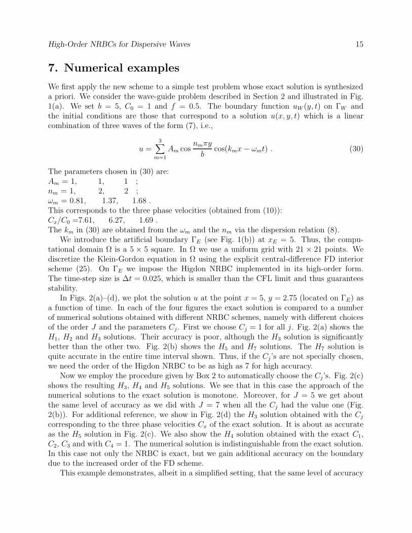
7. Numerical examples

We first apply the new scheme to a simple test problem whose exact solution is synthesizeda priori. We consider the wave-guide problem described in Section 2 and illustrated in Fig.1(a). We set b = 5, C0 = 1 and f = 0.5. The boundary function uW (y, t) on ΓW andthe initial conditions are those that correspond to a solution u(x, y, t) which is a linearcombination of three waves of the form (7), i.e.,

u =3∑

m=1

Am cosnmπy

bcos(kmx− ωmt) . (30)

The parameters chosen in (30) are:Am = 1, 1, 1 ;nm = 1, 2, 2 ;ωm = 0.81, 1.37, 1.68 .This corresponds to the three phase velocities (obtained from (10)):Cx/C0 =7.61, 6.27, 1.69 .The km in (30) are obtained from the ωm and the nm via the dispersion relation (8).

We introduce the artificial boundary ΓE (see Fig. 1(b)) at xE = 5. Thus, the compu-tational domain Ω is a 5 × 5 square. In Ω we use a uniform grid with 21 × 21 points. Wediscretize the Klein-Gordon equation in Ω using the explicit central-difference FD interiorscheme (25). On ΓE we impose the Higdon NRBC implemented in its high-order form.The time-step size is ∆t = 0.025, which is smaller than the CFL limit and thus guaranteesstability.

In Figs. 2(a)–(d), we plot the solution u at the point x = 5, y = 2.75 (located on ΓE) asa function of time. In each of the four figures the exact solution is compared to a numberof numerical solutions obtained with different NRBC schemes, namely with different choicesof the order J and the parameters Cj. First we choose Cj = 1 for all j. Fig. 2(a) shows theH1, H2 and H3 solutions. Their accuracy is poor, although the H3 solution is significantlybetter than the other two. Fig. 2(b) shows the H5 and H7 solutions. The H7 solution isquite accurate in the entire time interval shown. Thus, if the Cj’s are not specially chosen,we need the order of the Higdon NRBC to be as high as 7 for high accuracy.

Now we employ the procedure given by Box 2 to automatically choose the Cj’s. Fig. 2(c)shows the resulting H3, H4 and H5 solutions. We see that in this case the approach of thenumerical solutions to the exact solution is monotone. Moreover, for J = 5 we get aboutthe same level of accuracy as we did with J = 7 when all the Cj had the value one (Fig.2(b)). For additional reference, we show in Fig. 2(d) the H3 solution obtained with the Cj

corresponding to the three phase velocities Cx of the exact solution. It is about as accurateas the H5 solution in Fig. 2(c). We also show the H4 solution obtained with the exact C1,C2, C3 and with C4 = 1. The numerical solution is indistinguishable from the exact solution.In this case not only the NRBC is exact, but we gain additional accuracy on the boundarydue to the increased order of the FD scheme.

This example demonstrates, albeit in a simplified setting, that the same level of accuracy


obtained with parameter values Cj that are well-estimated can be achieved with ill-chosenparameter values but with an increased order J . Of course, increasing the order to ensurehigh accuracy is computationally expensive, and therefore it is usually beneficial to use thealgorithm given in Box 2.

We now consider another problem in the same wave-guide, again with b = 5, C0 = 1 and

-2

-1.5

-1

-0.5

0

0.5

1

1.5

0 2 4 6 8 10

u

t

Exact sol.J=1, C1=1J=2, Cj=1J=3, Cj=1

-2

-1.5

-1

-0.5

0

0.5

1

1.5

2

0 2 4 6 8 10

u

t

Exact sol.J=5, Cj=1J=7, Cj=1

(a) (b)

-2

-1.5

-1

-0.5

0

0.5

1

1.5

0 2 4 6 8 10

u

t

Exact sol.J=3J=4J=5

-2

-1.5

-1

-0.5

0

0.5

1

1.5

0 2 4 6 8 10

u

t

Exact sol.J=3, exact CjJ=4, exact Cj

(c) (d)

Figure 2: Solution of the three-wave test problem: u at the point x = 5, y = 2.75 (on ΓE)as a function of time. (a) Exact solution and the H1, H2 and H3 solutions with Cj = 1. (b)Exact solution and the H5 and H7 solutions with Cj = 1. (c) Exact solution and the H3,H4 and H5 solutions with automatically chosen Cj. (d) Exact solution and the H3 and H4

solutions with the exact Cj.


f = 0.5. The initial conditions are all zero, and the boundary function uW on ΓW is givenby

uW (y, t) =

cos[

π2r

(y − y0)]

if |y − y0| ≤ r & t ≤ t0

0 otherwise

(31)

Thus, the wave source on the west boundary is a cosine function in y with three parameters:its center location y0, its width r, and its time duration t0. We set y0 = 2.5, r = 1.5, andt0 = 0.5. In contrast to the previous test problem, the solution of this problem involves aninfinite number of modes and frequencies.

The computational parameters xE , ∆t and the grid are the same as in the previousexample. However, here we use the Higdon NRBC H4 on ΓE , with the four Cj’s obtainedautomatically by using the procedure given in Box 2. These turn out to be Cj/C0 = 1, 3.6,4.5 and 10.6.

We compare the solution obtained by the new scheme with two other solutions:

• A solution obtained in the same domain, but with the Higdon NRBC H1 on gE, usingC1 = 5, which in the middle of the range of the four Cj ’s mentioned above.

• A solution obtained in a domain twice as long, namely the domain 0 ≤ x ≤ 10,0 ≤ y ≤ 5, using a 42 × 21 grid with the same resolution. During the simulationtime the wave generated on ΓW does not reach the remote (east) boundary of thislarge domain, and thus the issue of spurious reflection is avoided altogether, regardlessof the boundary condition used on the remote boundary. Hence this will serve asa “reference solution” which is exact as far as the boundary-condition treatment isconcerned.

Fig. 3(a) shows the three solutions at time t = 4. In this and the next figures, the topplot is that of the reference solution, the middle plot corresponds to the solution obtained bythe new scheme with the H4 NRBC, and the lower plot describes the H1 solution. Both thecolors and the contour lines represent values of u. At time t = 4 the main bulk of the wavepacket generated on ΓW has not reached the boundary ΓE yet, and hence all three plots aresimilar.

Fig. 3(b) shows the three solutions at time t = 6. The wave packet has already passedthe boundary ΓE. The H4 solution is indistinguishable from the reference solution, whereasin the H1 solution spurious reflection is evident. Figs. 3(c) and 3(d) correspond to timest = 8 and t = 10, respectively. The reflected wave moves backwards in the H1 solution andpollutes the entire computational domain. On the other hand, the H4 solution exhibits thewave traces which are also present in the reference solution.

Finally we repeat this experiment while increasing the dispersion parameter by a factorof 20, i.e., we take f = 10. The group velocity decreases with increasing dispersion; hencethe wave packet will move much more slowly now. Also, the solution is expected to bemuch “richer,” being composed of many waves with different frequencies and phase speeds.Indeed, this is seen in Fig. 4(a), which illustrates the solution at time t = 12.5. The wave has


just reached the boundary ΓE , and the beginning of spurious reflection in the H1 solution isapparent. Figs. 4(b)–(d) show the solutions at times t = 15, t = 19 and t = 22.5, respectively.Again the H1 solution exhibits spurious reflection, while the H4 solution performs very wellin this high-dispersion case too.

8. Concluding Remarks

In this paper we have presented a new numerical procedure based on FDs, which allowsthe use of the Higdon NRBCs up to an arbitrarily high order. The scheme is coded onceand for all for any order; the order of the scheme is simply an input parameter. This addsan important computational tool for use in the solution of infinite domain time-dependentwave problems. Moreover, due to the generality of the Higdon NRBCs it is possible to usethis tool for problems with dispersive and layered media. We have focused on dispersivewaves in this paper, although the scheme is effective in the non-dispersive case as well. Wehave demonstrated that the high-order scheme, with the automatically-chosen parameters,performs very well in both the low and high dispersion regimes.

Related future work will include the adaptation of the proposed approach to more com-plicated configurations, such as exterior problems with a rectangular artificial boundary B,and three-dimensional problems. It should be remarked that no difficulties are expected inthe case where B has corners. The Higdon NRBCs do not involve mixed spatial derivatives,and thus the corner grid-point can arbitrarily be associated with one of the two straightedges that meet at this corner, and can be treated just as any other grid point on this chosenedge.

In addition, the high-order Higdon NRBCs will be applied to the Shallow Water Equa-tions (SWEs). The Shallow Water model serves as an important testbed for more compli-cated models in meteorology [38]. It would be interesting, among other things, to test theperformance of the high-order Higdon NRBCs when the nonlinear SWEs are used in thecomputational domain Ω.

An alternative formulation of the Higdon NRBCs is currently under development. Inthis formulation some auxiliary variables are introduced on the artificial boundary, in orderto eliminate all the high-order derivatives. This form of the NRBC has the advantages thatafter discretization it involves only degrees of freedom on the boundary B itself, that nohigh-order discrete schemes are needed, and that the history of the solution does not haveto be stored. As a result, it is more amenable, compared to the formulation presented inthis paper, for incorporation in a Finite Element scheme. This alternative formulation willbe reported in a future publication.

Acknowledgments

This work was supported by the U.S. National Research Council (NRC), the Office of NavalResearch (ONR), and the Naval Postgraduate School (NPS).


References

[1] D. Givoli, Numerical Methods for Problems in Infinite Domains, Elsevier, Amsterdam,1992.

[2] D. Givoli, “Non-Reflecting Boundary Conditions: A Review,” J. Comput. Phys., 94,1–29, 1991.

[3] S.V. Tsynkov, “Numerical Solution of Problems on Unbounded Domains, A Review,”Appl. Numer. Math., 27, 465–532, 1998.

[4] D. Givoli, “Exact Representations on Artificial Interfaces and Applications in Mechan-ics,” Appl. Mech. Rev., 52, 333–349, 1999.

[5] B. Engquist and A. Majda, “Radiation Boundary Conditions for Acoustic and ElasticCalculations,” Comm. Pure Appl. Math., 32, 313–357, 1979.

[6] A. Bayliss and E. Turkel, “Radiation Boundary Conditions for Wave-Like Equations,”Comm. Pure Appl. Math., 33, 707–725, 1980.

[7] J.B. Keller and D. Givoli, “Exact Non-Reflecting Boundary Conditions,” J. Comput.Phys., 82, 172–192, 1989.

[8] D. Givoli and J.B. Keller, “Non-Reflecting Boundary Conditions for Elastic Waves,”Wave Motion, 12, 261–279, 1990.

[9] J.P. Berenger, “A Perfectly Matched Layer for the Absorption of ElectromagneticWaves,” J. Comput. Phys., 114, 185–200, 1994.

[10] F. Collino, “High Order Absorbing Boundary Conditions for Wave Propagation Models.Straight Line Boundary and Corner Cases,” in Proc. 2nd Int. Conf. on Mathematical& Numerical Aspects of Wave Propagation, R. Kleinman et al., Eds., SIAM, Delaware,pp. 161-171, 1993.

[11] M.J. Grote and J.B. Keller, “Nonreflecting Boundary Conditions for Time DependentScattering,” J. Comput. Phys., 127, 52–65, 1996.

[12] M.J. Grote and J.B. Keller, “Nonreflecting Boundary Conditions for Elastic Waves,”SIAM J. Appl. Math., to appear.

[13] I.L. Sofronov, “Conditions for Complete Transparency on the Sphere for the Three-Dimensional Wave Equation,” Russian Acad. Dci. Dokl. Math., 46, 397–401, 1993.

[14] T. Hagstrom and S.I. Hariharan, “A Formulation of Asymptotic and Exact BoundaryConditions Using Local Operators,” Appl. Numer. Math., 27, 403–416, 1998.


[15] M.N. Guddati and J.L. Tassoulas, “Continued-Fraction Absorbing Boundary Conditionsfor the Wave Equation,” J. Comput. Acoust., 8, 139–156, 2000.

[16] D. Givoli, “High-Order Non-Reflecting Boundary Conditions Without High-OrderDerivatives,” J. Comput. Phys., 170, 849–870, 2001.

[17] D. Givoli and I. Patlashenko, “An Optimal High-Order Non-Reflecting Finite ElementScheme for Wave Scattering Problems,” Int. J. Numer. Meth. Engng., 53, 2389–2411,2002.

[18] J. Pedlosky, Geophysical Fluid Dynamics, Springer, New York, 1987.

[19] I.M. Navon, B. Neta and M.Y. Hussaini, “ A Perfectly Matched Layer Formulationfor the Nonlinear Shallow Water Equations Models: The Split Equation Approach,” toappear.

[20] R.L. Higdon, “Radiation Boundary Conditions for Dispersive Waves,” SIAM J. Numer.Anal., 31, 64–100, 1994.

[21] R.L. Higdon, “Absorbing Boundary Conditions for Difference Approximations to theMulti-Dimensional Wave Equation, Math. Comput., 47, 437–459, 1986.

[22] R.L. Higdon, “Numerical Absorbing Boundary Conditions for the Wave Equation,”Math. Comput., 49, 65–90, 1987.

[23] R.L. Higdon, “Radiation Boundary Conditions for Elastic Wave Propagation,” SIAMJ. Numer. Anal., 27, 831–870, 1990.

[24] R.L. Higdon, “Absorbing Boundary Conditions for Elastic Waves,” Geophysics, 56,231–241, 1991.

[25] R.L. Higdon, “Absorbing Boundary Conditions for Acoustic and Elastic Waves in Strat-ified Media,” J. Comput. Phys., 101, 386–418, 1992.

[26] R.A. Pearson, “Consistent Boundary Conditions for the Numerical Models of SystemsThat Admit Dispersive Waves,” J. Atmos. Sci., 31, 1418–1489, 1974.

[27] I. Orlanski, “A Simple Boundary Condition for Unbounded Hyperbolic Flows,” J.Comp. Phys., 21, 251–269, 1976.

[28] W.H. Raymond and H.L. Kuo, “A Radiation Boundary Condition for Multi-DimensionalFlows,” Q.J.R. Meteorol. Soc., 110, 535–551, 1984.

[29] M.J. Miller and A.J. Thorpe, “Radiation Conditions for the Lateral Boundaries ofLimited-Area Numerical Models,” Q.J.R. Meteorol. Soc., 107, 615–628, 1981.

[30] J.B. Klemp and D.K. Lilly, “Numerical Simulation of Hydrostatic Mountain Waves,” J.Atmos. Sci., 35, 78–107, 1978.


[31] M. Wurtele, J. Paegle and A. Sielecki, “The Use of Open Boundary Conditions withthe Storm-Surge Equations,” Mon. Weather Rev., 99, 537–544, 1971.

[32] R.M. Hodur, “The Naval Research Laboratory’s Coupled Ocean/Atmosphere MesoscalePrediction System (COAMPS),” Mon. Wea. Rev., 125, 1414-1430, 1997.

[33] X. Ren, K.H. Wang and K.R. Jin, “Open Boundary Conditions for Obliquely Prop-agating Nonlinear Shallow-Water Waves in a Wave Channel,” Comput. & Fluids, 26,269–278, 1997.

[34] T.G. Jensen, “Open Boundary Conditions in Stratified Ocean Models,” J. Marine Sys-tems, 16, 297–322, 1998.

[35] F.S.B.F. Oliveira, “Improvement on Open Boundaries on a Time Dependent NumericalModel of Wave Propagation in the Nearshore Region,” Ocean Eng., 28, 95–115, 2000.

[36] J.C. Strikwerda, Finite Difference Schemes and Partial Differential Equations,Wadsworth & Brooks, Pacific Grove, CA, 1989.

[37] B.P. Sommeijer, P.J. van der Houwen and B. Neta, “Symmetric Linear Multistep Meth-ods for Second Order Differential Equations with Periodic Solutions,” Applied NumericalMathematics, 2, 69–77, 1986.

[38] D.R. Durran, Numerical Methods for Wave Equations in Geophysical Fluid Dynamics,Springer, New York, 1999.


Captions for Figures

Fig. 1. Setup for the wave-guide problem: (a) the original problem in a semi-infinite waveguide; (b) the computational problem in a finite domain Ω.

Fig. 2. Solution of the three-wave test problem: u at the point x = 5, y = 2.75 (on ΓE) asa function of time. (a) Exact solution and the H1, H2 and H3 solutions with Cj = 1.(b) Exact solution and the H5 and H7 solutions with Cj = 1. (c) Exact solution andthe H3, H4 and H5 solutions with automatically chosen Cj. (d) Exact solution and theH3 and H4 solutions with the exact Cj .

Fig. 3. Solution of the west-source problem, dispersion parameter f = 0.5. Top plot —reference solution, middle plot — H4 solution, lower plot — H1 solution. Times: (a)t = 4, (b) t = 6, (b) t = 8, (b) t = 10.

Fig. 4. Solution of the west-source problem, dispersion parameter f = 10. Top plot —reference solution, middle plot — H4 solution, lower plot — H1 solution. Times: (a)t = 12.5, (b) t = 15, (b) t = 19, (b) t = 22.5.

High-order non-reflecting boundary conditions for dispersive waves

Documents

Transcript of High-order non-reflecting boundary conditions for dispersive waves