Finite difference method for transport of two-dimensional massless Dirac fermionsin a ribbon geometry

Alexis R. Hernandez1, 2 and Caio H. Lewenkopf3

1Instituto de Fısica, Universidade Federal do Rio de Janeiro, 21941-972 Rio de Janeiro, Brazil2Departamento de Fısica, Pontifıcia Universidade Catolica do Rio de Janeiro, 22452-970 Rio de Janeiro, Brazil

3Instituto de Fısica, Universidade Federal Fluminense, 24210-346 Niteroi, Brazil(Dated: October 29, 2012)

We present a numerical method to compute the Landauer conductance of non-interacting two-dimensional massless Dirac fermions in disordered systems. The method allows for the introductionof boundary conditions at the ribbon edges and to account for an external magnetic field. Byconstruction, the proposed discretization scheme avoids the fermion doubling problem. The methoddoes not rely on an atomistic basis and is particularly useful to deal with long-range disorder, whosecorrelation length largely exceeds the underlying material crystal lattice spacing. As an application,we study the case of monolayer graphene sheets with zigzag edges subjected long range disorder,which can be modeled by a single-cone Dirac equation.

PACS numbers: 72.10.-d,73.23.-b

I. INTRODUCTION

The growing research activity on the physical proper-ties of graphene1 as well as on topological insulators2,3

has increased the interest in methods to solve the twodimensional massless Dirac equation for various settings.In pristine graphene, two Dirac cones placed at the cor-ners of the Brillouin zone, frequently called valleys, pro-vide a good description of the electronic single-particlelow-energy spectrum. For topological insulators, two-dimensional massless Dirac excitations appear as edgestates between a non trivial tridimensional (3D) topolog-ical insulator and a trivial vacuum.

In distinction to analytical studies, that describe thesingle-particle properties of graphene by an effective two-dimensional Dirac Hamiltonian, almost all numericalanalysis employ an atomistic basis from the onset (forreviews, see for instance Refs. 4,5). Numerical studies ofthe electronic transport in graphene sheets and ribbonstypically use the tight-binding approximation to expressthe relevant Green’s functions in terms of atomic sitepositions.6–8 This basis choice has the advantage of sim-plicity, but its computational cost increases very fast withsystem size. For the cases where short range disorder isimportant and an accurate description of the system atsmall length scales is necessary, the use of an atomic basisis not only the simplest, but also the most natural choice.The picture is very different in systems characterized bylong range disorder and/or subjected to a smooth back-ground electrostatic potential. In these cases, interval-ley scattering is absent1,4 and the system description interms of a single Dirac cone is very accurate. Here, a nu-merical method that starts with the Dirac Hamiltonian iscertainly computationally more efficient and very likelyto be more insightful. The development of such methodis the main goal of this paper.

Topological insulators2,3 have rekindled the interest onthe research related to concepts of topological order, of-

ten used to characterize the singular behavior of the in-teger and fractional quantum Hall effects. Topologicalinsulators are mainly characterized by the presence ofchiral boundary states. It was recently discovered a se-ries of next generation 3D topological insulators. Thesematerials exhibit a very simple band structure with asingle Dirac cone. The non trivial topological nature ofthese materials makes their boundary states more ro-bust against disorder than the corresponding ones ingraphene. In lattice quantum field theory the introduc-tion of boundary conditions has been guided by the in-dex theorem9 and by the phenomenological presence ofAdler-Bell-Jackiw (chiral) anomalies10 observed in highenergy experiments. In this context, it has been shownthat nonlocal boundary conditions are necessary to re-produce the observed anomaly. For graphene and topo-logical insulators the boundary conditions are local andwell understood.11,12

In this study we combine two finite differencemethods,13,14 developed in the context of lattice gaugetheory, to numerically compute the scattering matrix oftwo-dimensional massless Dirac particles. Our methodavoids the fermion doubling problem and allows to intro-duce suitable boundary conditions at the system edges.To illustrate its utility we consider boundary conditionsmimicking the zigzag edges of a graphene sheet.11 In-spired on the procedure proposed by Tworzydlo andcollaborators,15 we develop a method to compute trans-port properties of massless Dirac particles in systemswith different edge boundary conditions. In addition,the method we put forward also allows to account forthe presence of an external magnetic field.

We apply the method to compute the average conduc-tivity at the charge neutrality point of large disorderedgraphene systems. We consider diagonal disorder andcompute the average conductivity by taking disorder en-semble averages. We scale the conductivity with the sys-tem size to numerically obtain the corresponding univer-sal curve, a matter of an intense controversy in the recent

arX

iv:1

210.

7037

v1 [

cond

-mat

.mes

-hal

l] 2

6 O

ct 2

012

2

literature.4,16–18 We also study the conductance fluctua-tions at the charge neutrality point, providing numericalevidence of a non universal behavior.

The presentation is organized as follows. In Sec. IIwe review the discretization strategies used to solve theDirac Hamiltonian. In Sec. III we construct a discretiza-tion procedure to calculate the Landauer conductanceof two-dimensional massless Dirac particles confined to aribbon with boundary conditions that mimic zigzag edgesin graphene. Ballistic transport is discussed in Sec. IV,where we apply the method to reproduce the standardresults found in the literature. In Sec. V we apply thetransfer matrix method to study diffusive transport inlong-range disordered graphene stripes. Next, we showhow to include a magnetic field in the method and com-pute the conductance at the (anomalous) quantum Hallregime in Sec. VI. Finally, we present our conclusions andoutlook in Sec. VII.

II. MASSLESS DIRAC EQUATION IN ALATTICE

Let us consider the two-dimensional massless DiracHamiltonian

H = −i~v(σx∂x + σy∂y) + U(r), (1)

where v is the velocity of the massless Dirac fermions,σx and σy are Pauli matrices, and U(r) is the potentialenergy landscape. The eigenvalue problem reads

HΨ = EΨ , (2)

where E is the fermion energy and Ψ is a two-component(spinor) wave function of the form

Ψ =

(ψ

ψ

). (3)

For graphene, the two components of the spinor Ψ cor-respond to the electron wave function amplitudes at eachof the two intercalated triangular lattices, denoted by Aand B, that form the honeycomb lattice. Equation (1) isthe effective low energy graphene Hamiltonian for elec-trons in the vicinity of the Brillouin zone K-point, calledK-valley. By replacing σy → −σy one obtains the corre-sponding equation for the K ′-valley.1

In the case of topological insulators, the spinor com-ponents of Ψ are interpreted as the electron z-axis spinprojection.

Our aim is to find a suitable lattice representation forthe H operator in Eq. (1). The square lattice, that isvery efficient to discretize a two-dimensional SchrodingerHamiltonian, would be the most natural candidate. How-ever, it is well established in the lattice gauge theoryliterature13,14,19 that this choice leads to wrong results.

Let us understand this statement and motivate thediscretization scheme we propose by discussing the typi-cal problems that arise in the discretization of the Dirac

equation. For the sake of simplicity, let us consider thesimplest possible setting, namely, a one-dimensional sta-tionary massless fermion field. The Dirac equation reads

− i~vσx∂xΨ(x) = EΨ(x) . (4)

Despite the simplicity of Eq. (4), its solution by dis-cretization requires some care. The naive evaluation ofthe derivative as ∂xΨ(x) = [Ψ(x + ∆) − Ψ(x)]/∆ is un-suited, since it produces a non-Hermitian Hamiltonian.The reason is that the left and the right hand sides ofEq. (4) are evaluated at different points, namely x andx + ∆/2. The evaluation of ∂xΨ(x) in Eq. (4) by tak-ing ∂xΨ(x) = [Ψ(x + ∆) − Ψ(x − ∆)]/2∆ also fails. Inthis case, one finds an Hermitian Hamiltonian, but witha wrong spectrum: The number of fermions in the firstBrillouin zone is doubled. This is the so-called fermiondoubling problem. It arises because the lattice size ∆ ishalf of the spacing between the points used to estimate∂xΨ(x).14

To correctly solve Eq. (4) by discretization, it is nec-essary to evaluate ∂xΨ(x) and Ψ(x) at the same meshposition and to use a single effective lattice spacing. Be-low, we review two different strategies that satisfy theserequirements.Stacey discretization:14 The fermionic fields are deter-

mined at the lattice points xm = m∆ and the Diracequation is evaluated at the lattice midpoints, namely,m∆ + ∆/2.

In other words, since the derivative is ∂xΨ(x+ ∆/2) =[Ψ(x + ∆) − Ψ(x)]/∆ and both sides of Eq. (4) mustbe evaluated at the same position, the fermionic fieldsare approximated by the average between adjacent sites,namely, Ψ(x+ ∆/2) = [Ψ(x+ ∆) + Ψ(x)]/2.

The resulting system of coupled finite difference equa-tions reads

− i~v∆

(ψm+1 − ψmψm+1 − ψm

)=E

2

(ψm+1 + ψmψm+1 + ψm

), (5)

where ψm = ψ(m∆) and ψm = ψ(m∆).Susskind discretization:13 This scheme is based on a

slightly more involved construction than the one just pre-

sented. The fermionic fields, ψ and ψ, are defined in twointercalated lattices. The lattices have a lattice parame-ter ∆ and are offset by a distance ∆/2.

Let us consider the spinor component ψ to be de-

fined at xm = m∆ and the component ψ defined atxm = m∆ − ∆/2. Given that σx is non diagonal, onecan evaluate the upper component of Eq. (4) at x andthe lower component at x−∆/2.

The Dirac equation, Eq. (4), is approximated by thecoupled finite difference equations

− i~v∆

(ψm+1 − ψmψm − ψm−1

)= E

(ψmψm

), (6)

where ψm = ψ(m∆) and ψm = ψ(m∆ − ∆/2). No-

tice that the definitions of ψm and ψm for the Susskind

3

discretization differ from the ones used in the Stacey dis-cretization scheme.

In summary, both reviewed discretization proceduresfulfill the desired goals: They render Hermitian Hamilto-nians with the correct spectrum at the continuum limit,eliminating the fermion doubling problem.

III. TRANSFER MATRIX DISCRETIZATION

In this section we describe how to combine the trans-fer matrix method and the discretization schemes pre-sented above to compute the Landauer conductance forgraphene ribbons with zigzag edges. We use the Susskinddiscretization along the ribbon transversal direction, be-cause it allows for the implementation of zigzag-likeboundary conditions at the ribbon edges. Along the lon-gitudinal direction, we use the Stacey scheme, since it canbe nicely combined with the transfer matrix method.

We consider a geometry where source and drain areplaced at two opposite sides of a rectangular sheet. Thegraphene sheet has a length L in the direction connectingsource and drain, that is longitudinal to the electronicpropagation, and a transversal width W .

We take the x-axis along the longitudinal direction,and write Eq. (1) as

∂xΨ = (−iσz∂y − iσxV/∆)Ψ (7)

where V = (U −E)∆/~v. The Landauer conductance isobtained by solving Eq. (7) in a lattice using the transfermatrix method. For notational convenience, the latticesize ∆ is accounted for in the definition of V , a dimen-sionless quantity.

The graphene zigzag-like boundary conditions are im-

plemented by making ψ = 0 at y = 0 and ψ = 0 aty = W , corresponding to opposite edges of the ribbon.11

In Appendix A we show how to implement the finite dif-ference method to address armchair-like boundary con-ditions.

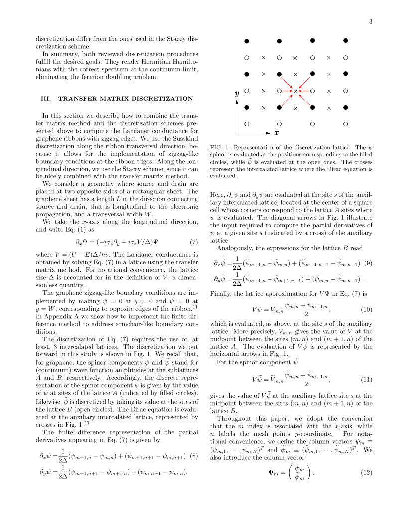
The discretization of Eq. (7) requires the use of, atleast, 3 intercalated lattices. The discretization we putforward in this study is shown in Fig. 1. We recall that,

for graphene, the spinor components ψ and ψ stand for(continuum) wave function amplitudes at the sublatticesA and B, respectively. Accordingly, the discrete repre-sentation of the spinor component ψ is given by the valueof ψ at sites of the lattice A (indicated by filled circles).

Likewise, ψ is discretized by taking its value at the sites ofthe lattice B (open circles). The Dirac equation is evalu-ated at the auxiliary intercalated lattice, represented bycrosses in Fig. 1.20

The finite difference representation of the partialderivatives appearing in Eq. (7) is given by

∂xψ =1

2∆(ψm+1,n − ψm,n) + (ψm+1,n+1 − ψm,n+1) (8)

∂yψ =1

2∆(ψm+1,n+1 − ψm+1,n) + (ψm,n+1 − ψm,n).

FIG. 1: Representation of the discretization lattice. The ψspinor is evaluated at the positions corresponding to the filled

circles, while ψ is evaluated at the open ones. The crossesrepresent the intercalated lattice where the Dirac equation isevaluated.

Here, ∂xψ and ∂yψ are evaluated at the site s of the auxil-iary intercalated lattice, located at the center of a squarecell whose corners correspond to the lattice A sites whereψ is evaluated. The diagonal arrows in Fig. 1 illustratethe input required to compute the partial derivatives ofψ at a given site s (indicated by a cross) of the auxiliarylattice.

Analogously, the expressions for the lattice B read

∂xψ =1

2∆(ψm+1,n − ψm,n) + (ψm+1,n−1 − ψm,n−1) (9)

∂yψ =1

2∆(ψm+1,n − ψm+1,n−1) + (ψm,n − ψm,n−1) .

Finally, the lattice approximation for VΨ in Eq. (7) is

V ψ = Vm,nψm,n + ψm+1,n

2, (10)

which is evaluated, as above, at the site s of the auxiliarylattice. More precisely, Vm,n gives the value of V at themidpoint between the sites (m,n) and (m + 1, n) of thelattice A. The evaluation of V ψ is represented by thehorizontal arrows in Fig. 1.

For the spinor component ψ

V ψ = Vm,nψm,n + ψm+1,n

2, (11)

gives the value of V ψ at the auxiliary lattice site s at themidpoint between the sites (m,n) and (m + 1, n) of thelattice B.

Throughout this paper, we adopt the conventionthat the m index is associated with the x-axis, whilen labels the mesh points y-coordinate. For nota-tional convenience, we define the column vectors ψm ≡(ψm,1, · · · , ψm,N )T and ψm ≡ (ψm,1, · · · , ψm,N )T . Wealso introduce the column vector

Ψm =

(ψmψm

). (12)

4

that represents the spinor Ψ of Eq. (3) evaluated at bothA and B sublattices for a given m, corresponding to a

x = m∆. In Fig. 1, single columns represent Ψm spinorsof different m’s.

Plugging (8) to (11) in Eq. (7) we obtain

(I + N+)(ψm+1 −ψm) =i(I− N+)(ψm+1 +ψm)− iVm(ψm+1 + ψm) (13)

(I + N−)(ψm+1 − ψm) =i(I− N−)(ψm+1 + ψm)− iVm(ψm+1 +ψm)

where I is the N ×N identity matrix, N+ and N− are super- and subdiagonal matrices, namely, (N+)nn′ = δn,n′−1,

(N−)nn′ = δn,n′+1, while Vm and Vm have matrix elements given by (Vm)nn′ = Vmnδnn′ and (Vm)nn′ = Vmnδnn′ .By writing Eq. 13 in terms of Ψm and Ψm+1,(

(I + N+)− i(I− N+) iVmiVm (I + N−)− i(I− N−)

)Ψm+1 =

((I + N+) + i(I− N+) −iVm

−iVm (I + N−) + i(I− N−)

)Ψm.

(14)

allows us to identify the transfer matrix M defined by

Ψm+1 = MmΨm, (15)

namely,

Mm =I− iXmI + iXm

, (16)

where

Xm = J−1

(−(I− N+) Vm

Vm −(I− N−)

)(17)

and

J =

(I + N+ 0

0 I + N−). (18)

We define the current operator in the x-direction as

Jx =1

2v

(0 J−J+ 0

), (19)

with J+ = I + N+ and J− = I + N−. In Appendix Bwe show that this choice of Jx guarantees charge conser-vation. As a consequence of the zigzag boundary condi-tions, our discretization method does not preserve sym-plectic symmetry. This is in contrast with the methodput forward in Ref. 15, that deals with periodic bound-ary conditions along the y-direction and treats infinitelywide systems.

A. Landauer conductance

The transfer matrix of the whole graphene sheet can, in

principle, be computed using M =∏Mm=1 Mm. However,

it is well known that this scheme is numerically unstable:It produces both exponentially growing and exponen-tially decaying eigenvalues. Limited numerical accuracy

prevents one from retaining both sets of eigenvalues.15

The numerical instability problem is solved by workingwith compositions of unitary scattering matrices,15,21 atthe expense of introducing additional diagonalizationsthat slow down the computation. We adopt the schemeproposed in Ref. 15 with a small modification, which webriefly describe in what follows.

In order to translate the transfer matrix M into a uni-tary scattering matrix

S =

(r t′

t r′

)(20)

one needs to solve the equation

Φrighta = MΦleft

a (21)

with

Φrighta =

∑l

tabφ+b , Φleft

a = φ+a +

∑l

rabφ−b . (22)

for each asymptotic propagating channel a at the source(left) or drain (right) contacts. We consider the situationwhere all channels are open. This is similar to the set-ting where the contacts have a high doping and a largedensity of states to realistically model standard metalliccontacts,22 minimizing the effect of a contact resistance.

In the large wave vector limit, the states φ±a (a =1, 2, ..., N) are given by the 2N eigenstates of the currentoperator Jx, normalized such that each mode carries thesame current. That is

φ±a = j−1/2a

(ψa±ψa

)(23)

where ψa and ja are given by

J+ψa = jaψa

J−ψa = jaψa (24)

with (ψa)n = (ψa)N+1−n.

5

To obtain a closed-form expression for S in terms ofM, we write M in the basis of channels φ±k through thesimilarity transformation

Mm = RMm R−1 (25)

where

(R−1)2N×2N = (φ+1 , · · · , φ

+N , φ

−1 , · · · , φ

−N ). (26)

This R is not the same as the one used in Ref. 15: We usea different transversal discretization scheme and R is de-fined to facilitate the projection of single-contributions tothe transmission from different channels. The later char-acteristic is very useful for the method implementation,as justified in the next section.

The spinor degrees of freedom of M are separated intofour N ×N blocks,

M =

(M++ M+−

M−+ M−−

)(27)

and follow the same strategy employed in Sec. III.b of

Ref. 15 to write the S matrix in terms of the M sub-blocks. Finally, the conductance is evaluated as usual bythe Landauer formula

G =gsgve

2

hT (28)

where gs and gv stand for the spin and valley degeneraciesand T is the transmission, namely, T = tr[t†t].

B. Spurious mode and its elimination

Let us discuss the properties of the transfer matrix forthe simple case of a pristine graphene ribbon with zigzagedges. Due to translation invariance, all transversal slicesm are equivalent, and the transfer matrix MPUC = Mm,corresponding to the primitive unit cell, is sufficient todescribe the transport.

For a given energy E, the transfer matrix MPUC hasNch eigenvalues of the form eika∆ with ka real. Hence,Nch gives the number of propagating channels and ka isassociated with the wave number along the propagationdirection of the corresponding channel. This allows us toobtain the dispersion relation for a graphene ribbon. Fora given ribbon width W , we vary the energy E in smallsteps and calculate the eigenvalues and eigenchannels ofMPUC. The result for the discretization of the K-valleyis shown in Fig. 2.

The band structure shown in Fig. 2 coincides withthe results obtained by the continuum limit treatmentof the zigzag boundary conditions of Ref. 11 around theK valley. As expected, the low energy states are also ingood agreement with those of the nearest-neighbor tight-binding model. The only discrepancy is the appearanceof an “extra” mode around k∆/π ≈ 1. To understand

−1.0 −0.5 0.0 0.5 1.0

−0.6

−0.4

−0.2

0.0

0.2

0.4

0.6

k!/"

E[e

V]

k∆/π

E[e

V]

FIG. 2: Band structure of Dirac fermions in a infinite ribbonof width W = 100∆ with zigzag-like boundary conditionsobtained using the method described in the text. The energyscale is set by fixing ∆ = 10a0, where a0 = 1.42 A is thecarbon-carbon bond length in graphene.

its nature, it is convenient to analyze the correspondingeigenstate. This is done next.

The transfer matrix MPUC has two zero-energy eigen-modes, whose typical transversal wave function ampli-tudes are shown in Fig. 3. The “smooth” mode corre-sponding to Fig. 3a is similar to the analytical solutionpresented in Ref. 11. In addition, we find a spuriousmode that oscillates on the scale of the lattice size dis-cretization, shown in Fig. 3b.

In finite difference calculations, states showing oscil-lations at the scale of lattice size are expected to bebadly described by the discretized equation. Usually,they correspond to the states of higher energy in thespectrum. The general rule is that the first half or so ofthe computed states are well described by the discretiza-tion. Hence, provided one is interested in the low en-ergy part of the spectrum, the inaccurate high frequencystates do not cause any problem. These observationsdo not apply here. For example, in the Tworzydlo andcollaborators15, that employ a Stacey-like discretizationto handle the fermion doubling problem, the effective lat-tice size is doubled to evaluate the derivatives of Ψ. Asa consequence, the high energy states at the top of thespectrum are poorly described and spurious states arise.To eliminate these spurious states, very long filters ateach side of his graphene stripe are introduced.

In our case, the Susskind discretization preserves thelattice size, however the peculiar nature of the edge state,characteristic of ribbons with zigzag edges, pulls downthe energy of the maximally transversal oscillating state.The combined oscillations in both sublattices render adispersionless mode in the finite difference representationof the momentum operator.

To eliminate (up to a very good accuracy) the spuri-ous state illustrated in Fig. 3b, we simply eliminate the

6

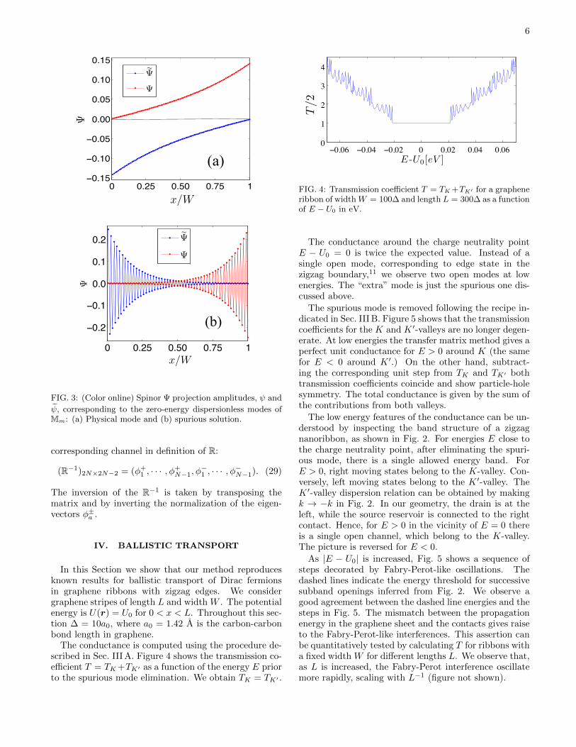
0 0.25 0.50 0.75 1−0.15

−0.10

−0.05

0.00

0.05

0.10

0.15

x [W ]

!

! A

! B

(a)

~

x/W

0 0.25 0.50 0.75 1

−0.2

−0.1

0.0

0.1

0.2

x [W ]

!

! A

! B

(b)

~

x/W

FIG. 3: (Color online) Spinor Ψ projection amplitudes, ψ and

ψ, corresponding to the zero-energy dispersionless modes ofMm: (a) Physical mode and (b) spurious solution.

corresponding channel in definition of R:

(R−1)2N×2N−2 = (φ+1 , · · · , φ

+N−1, φ

−1 , · · · , φ

−N−1). (29)

The inversion of the R−1 is taken by transposing thematrix and by inverting the normalization of the eigen-vectors φ±a .

IV. BALLISTIC TRANSPORT

In this Section we show that our method reproducesknown results for ballistic transport of Dirac fermionsin graphene ribbons with zigzag edges. We considergraphene stripes of length L and width W . The potentialenergy is U(r) = U0 for 0 < x < L. Throughout this sec-tion ∆ = 10a0, where a0 = 1.42 A is the carbon-carbonbond length in graphene.

The conductance is computed using the procedure de-scribed in Sec. III A. Figure 4 shows the transmission co-efficient T = TK+TK′ as a function of the energy E priorto the spurious mode elimination. We obtain TK = TK′ .

!0.06 !0.04 !0.02 0 0.02 0.04 0.060

1

2

3

4

E -U0[eV ]

TT

/2

FIG. 4: Transmission coefficient T = TK +TK′ for a grapheneribbon of widthW = 100∆ and length L = 300∆ as a functionof E − U0 in eV.

The conductance around the charge neutrality pointE − U0 = 0 is twice the expected value. Instead of asingle open mode, corresponding to edge state in thezigzag boundary,11 we observe two open modes at lowenergies. The “extra” mode is just the spurious one dis-cussed above.

The spurious mode is removed following the recipe in-dicated in Sec. III B. Figure 5 shows that the transmissioncoefficients for the K and K ′-valleys are no longer degen-erate. At low energies the transfer matrix method gives aperfect unit conductance for E > 0 around K (the samefor E < 0 around K ′.) On the other hand, subtract-ing the corresponding unit step from TK and TK′ bothtransmission coefficients coincide and show particle-holesymmetry. The total conductance is given by the sum ofthe contributions from both valleys.

The low energy features of the conductance can be un-derstood by inspecting the band structure of a zigzagnanoribbon, as shown in Fig. 2. For energies E close tothe charge neutrality point, after eliminating the spuri-ous mode, there is a single allowed energy band. ForE > 0, right moving states belong to the K-valley. Con-versely, left moving states belong to the K ′-valley. TheK ′-valley dispersion relation can be obtained by makingk → −k in Fig. 2. In our geometry, the drain is at theleft, while the source reservoir is connected to the rightcontact. Hence, for E > 0 in the vicinity of E = 0 thereis a single open channel, which belong to the K-valley.The picture is reversed for E < 0.

As |E − U0| is increased, Fig. 5 shows a sequence ofsteps decorated by Fabry-Perot-like oscillations. Thedashed lines indicate the energy threshold for successivesubband openings inferred from Fig. 2. We observe agood agreement between the dashed line energies and thesteps in Fig. 5. The mismatch between the propagationenergy in the graphene sheet and the contacts gives raiseto the Fabry-Perot-like interferences. This assertion canbe quantitatively tested by calculating T for ribbons witha fixed width W for different lengths L. We observe that,as L is increased, the Fabry-Perot interference oscillatemore rapidly, scaling with L−1 (figure not shown).

7

!0.06 !0.04 !0.02 0 0.02 0.04 0.060

1

2

3

4

E -U0[eV ]

TK -valley

(a)(a)

T

!0.06 !0.04 !0.02 0 0.02 0.04 0.060

1

2

3

4

E-U0[eV ]

T

K !-valley

(b)(b)

T

FIG. 5: Transmission T for graphene ribbons of width W =100∆ and length L = 300∆ as a function of E − U0 in eVusing a massless Dirac equation centered at the (a) K-pointand (b) K′-point. The vertical dashed lines are placed at thethreshold energies of the propagating modes in the depictedenergy interval.

Due to their rough edges, such Fabry-Perot interfer-ence patterns are unlikely to be observed in lithographicgraphene nanoribbons. The situation is more promisingin smooth edge graphene ribbons, made by unzippingcarbon nanotubes.23

We note that alternative discretization schemes canbe used to construct a transfer matrix to compute thetransport of Dirac fermions in ribbons with armchair-like boundary conditions,11 and possibly also for chiralboundary conditions.24 Our motivation to focus only atthe zigzag case is twofold: (i) In distinction to the others,this boundary condition does not mix the valleys isospins.This allows to solve the problem in the K and K ′-valleysseparately, which speeds up the computation by a factorabout 23. (ii) The method was put forward to computetransport properties of realistically large samples in thepresence of long range disorder, for which the sampleboundaries should not play a key role.

V. MESOSCOPIC EFFECTS

The electronic transport in graphene at the chargeneutrality point has been the subject of intense exper-imental and theoretical work, as reviewed, for instancein Refs. 4,5. While it is by now established that in goodmobility graphene samples the observed conductivity σis of the order of e2/h, its value still depends on sample

disorder. In the diffusive regime, where the system sizeL is much larger than the electron mean free path `, σis expected to show a weak system size dependence. Inthe ballistic case, where L . `, the conductivity dependsstrongly on the system geometry and it is more appropri-ate to describe transport properties by the conductivity.It is likely that the graphene samples used in many of thereported experiments correspond to a ballistic-diffusivecrossover.4

In this Section we apply the finite difference methodto compute the graphene conductivity σ at the chargeneutrality point in the presence of long range disor-der. We obtain the expected anti-weak localization re-lation between σ and the system size,25 namely, 〈σ〉 =(gsgve

2/πh) ln(L/`). Next, we study the conductancefluctuations at the charge neutrality point and show thatthey are not universal.

The transfer matrix approach gives the two-terminalconductance G. The conductivity is obtained from therelation σ = (L/W )〈G〉, where 〈· · · 〉 stands for a disorderensemble average. Since we assume that there is no inter-valley scattering, there is no need to choose a finite corre-lation length for the potential fluctuations,15 in distinc-tion to other previous theoretical analysis.4,6,7,17,18,26–28

As in Ref. 15 we let the potential at each lattice pointfluctuate independently. More specifically, we drawUm,n from an uniform distribution within the interval[−δU, δU ].

We compute the conductivity for 103 realizations fordifferent values of δU , corresponding to different meanfree paths. We assume that the conductivity follows therelation15

σ

G0=

1

πln

[L

`∗(δU)

]+ C(δU)

∆

L, (30)

where G0 = gsgve2/h. Here the first term at the right-

hand side is just the weak anti-localization relation with`∗(δU) associated with `, while the second one accountsfor finite size corrections and/or a contact resistance. Forevery set of disorder realizations with a given value of δUwe vary the system size (L = W = 30, 60, 90, and 120∆)and compute 〈G(L)〉. With the help of (30), these dataare used to find `∗(δU) and C(δU).

Figure 6 shows

σ =1

πln

[L

`∗(δU)

](31)

obtained from the simulations described above. We re-mark that our method allows to explore a much largerrange of L/`∗ than any previous study.

The current understanding of the conductance fluc-tuations is less clear. Analytical works make predic-tions of universal conductance fluctuations (UCF) ingraphene.29,30 However, since these results rely on di-agrammatic expansions in powers of (kF `)

−1, they areapplicable for large doping but are hardly relevant toexplain the fluctuations at the vicinity of the charge neu-trality point. The available experimental data31 do not

8

FIG. 6: Conductivity σ at the charge neutrality point as afunction of system size L/`∗. Points correspond to differ-ent system sizes L = W = 30, 60, 90, and 120∆ and disorderstrengths δU = 2, 4, 6, and 8. The dashed line is given byEq. (31). The lattice spacing is ∆ = 5a0.

provide a very consistent picture, possibly indicating anabsence of UCF in graphene at zero doping.

An early numerically work6 studied conductance fluc-tuation in graphene in the presence of short range dis-order. More recently, a systematic analysis of theconductance fluctuations in graphene sheets has beenperformed.32 The study reports conductance fluctuationsas a function of doping, system size L/ξ, and disor-der strength. The authors consider graphene sheetswith transversal periodic boundary conditions (no edges)and use the finite difference method put forward byTworzydlo and collaborators.15

We analyze the variance of the conductance fluctua-tions, var(G) = 〈G2〉 − 〈G〉2, at the charge neutralitypoint as a function of L`∗. In distinction to Ref. 15, wefind no evidence of universal conductance fluctuations,even going deep into the diffusive regime L/`∗ � 1. Asstated above, we believe that the strong discrepancy be-tween our results and the prediction from diagrammaticperturbation theory,29,30 is due to the breakdown of theperturbation theory when kF `� 1, that is, when one ap-proaches the charge neutrality point. In such situation,numerical simulation such as the one presented here givethe correct way to approach the problem.

VI. INCLUSION OF A MAGNETIC FIELD

In this section we show how to modify the transfer ma-trix discretization scheme presented in Sec. III to accountfor the presence of an external magnetic field. This allowsone to calculate (in the single-particle picture) the con-ductance of ballistic and long range disordered graphenesheets for arbitrary values of a perpendicularly applied

FIG. 7: Conductance fluctuations variance var(G/G0) as afunction of system size L/`∗.

magnetic field.As standard, an external magnetic field is introduced

in the Dirac Hamiltonian by minimal coupling.33 In whatfollows, we consider the vector potential A = (−By, 0, 0)that corresponds to the constant magnetic field B = Bz.It is important to mention that, since the discretiza-tion schemes along the x and y directions are different,gauge invariance is broken and the choice of A has tobe cautiously made. The minimal coupling substitutionp→ p− (e/c)A modifies Eq. (7) to

(∂x − ieBy/~c)Ψ = −i(σz∂y + σxV/∆)Ψ . (32)

Note that the magnetic field does not couple differentvalley pseudospin projections. Equation (32) refers tothe K-valley. As before, by replacing σy → −σy oneobtains the corresponding equation for the K ′-valley.

The transfer matrix discretization for Eq. (32) is con-structed in the same way as the one presented in Sec III.The expression for Mm is given by Eq. (16), but now Xmis given by

Xm = J−1

(N+ − I− iπφ

2φ0D J+ Vm

Vm N− − I− iπφ2φ0

D J−

)(33)

where φ = B∆2 is the magnetic flux through a squareunit cell (lattice A or B), φ0 = h/2ec is the magnetic fluxquantum, while D and D are diagonal matrices, whosematrix elements read Dnn′ = nδnn′ and Dnn′ = (n −1/2)δnn′ .

To illustrate the results that can be obtained by thismethod, we compute the Landauer conductance of a bal-listic graphene sheet in the anomalous quantum Hallregime.

Figure 8 shows the K-valley conductance for a rect-angular graphene ribbon geometry, where L = 400∆,W = 200∆ and ∆ = a0, subjected to different perpen-dicular B fields. The energy axis is scaled by (B0/B)1/2,

9

where B0 = 20 T to make evident that the Landaulevel energies EN scale with B−1/2, as expected for Diracfermions.1 More precisely, EN = ~ωcN1/2, where the cy-clotron frequency ωc = vF (2eB/~)1/2. The transmissionsteps in Fig. 8 nicely coincide with the Landau level en-ergies. The different B-field conductance curves stronglyoverlap. We observe that as E is increased, the conduc-tance steps become less well-defined. This behavior isparticularly evident for B = 20 T and become less pro-nounced as B is increased. The interpretation is thatwith increasing B, the edge states become more local-ized and hence tunneling between edges, which destroysquantization, is suppressed.

0 0.02 0.04 0.06 0.08 0.10

2

4

6

8

10

12

14

(E−U0)/B1/2 [eV/T]

G/G

0

B=20 TB=40 TB=80 T

W=200 ! L=400 ! !=a0

(E-U0)/(B/B0)1/2 [eV]

T

B=80 TB=40 TB=20 T

FIG. 8: Transmission T for different magnetic field values asa function of E for L = 400a0 and W = 200a0. To make themagnetic field dependence of the Landau levels in grapheneexplicit, the energy axis is scaled by (B0/B)1/2, with B0 =20T . After scaling all curves largely coincide. For the sake ofclarity, the transmission for B = 40 T is offset by +2 units,while T for B = 80 T is offset by +4 units.

For the system we analyze, the K ′-valley transmis-sion coefficient for E − U0 > 0 is TK′ = TK − 1. Thecorresponding figure is not shown, but bears a stronganalogy to the situation we discussed in Sec. IV. Thefull conductance is given by the contribution of bothK and K ′ valley pseudospin components, namely G =(gse

2/h)(TK +TK′) and consistent with the result foundin the literature.1,33

VII. CONCLUSION AND OUTLOOK

In this paper we put forward a numerical method tocalculate transport properties of two-dimensional mass-less Dirac particles. The numerical procedure combinesa finite difference description of the Dirac equation witha current conserving transfer matrix formalism. Themethod is useful to study the Landauer conductance in

graphene and surface states in 3D topological insulators.The use of a finite difference description of the Dirac

equation to calculate transport coefficients under givenboundary conditions demands tailormade discretizationschemes. We consider a system with a rectangular ge-ometry. In the longitudinal direction, parallel to the axisconnecting source and drain, a Stacey-like discretizationallows us to implement the transfer matrix formalism. Inthe transversal direction, a Susskind-like discretizationmakes possible the inclusion of zigzag-like edge bound-ary conditions. By construction, our method avoids thefermion doubling problem.

The proposed method becomes numerically advanta-geous with respect to the standard ones, that employ anatomic basis, when treating systems where long rangedisorder is dominant. In this case, the disorder range ξsets the discretization length scale. That is, ∆ . ξ in-stead of ∆ ∼ a0 as in any atomistic basis discretization.For a ribbon of length L and width W , the computationtime of transport properties scales with (L/∆)×(W/∆)3.Hence, for a given geometry, our discretization method isof the order of (ξ/a0)4 times computationally faster thanstandard atomistic ones.

To illustrate how the method works, we analyzed thetransport properties of ballistic and diffusive grapheneribbons in the absence of magnetic field, as well as theanomalous quantum Hall plateaus in a graphene sampleunder a strong perpendicular magnetic field.

We believe that the most promising features of ourmethod is that it allows considering different kinds ofboundary conditions. The present study addresses thecase of zigzag-like edges, but the transversal discretiza-tion can be modified to mimic arm-chair (see AppendixA) and chiral edges, as well as non-trivial periodic bound-ary conditions suitable to describe surface states of cer-tain topological insulators. We believe our method canbe very helpful for the study of issues related to the in-triguing nature of boundaries in Dirac systems.

Acknowledgments

We thank Eduardo Mucciolo and Nancy Sandler foruseful discussions. This work is supported in part by theBrazilian funding agencies CNPq and FAPERJ.

Appendix A: Armchair graphene ribbons

In this Appendix we modify the discretization proce-dure presented in Sec. III to address graphene ribbonswith armchair-like edges. To satisfy the boundary condi-tions of such systems one needs to mix both K and K ′

Dirac-valley components,1,11 namely,

Ψ =

(ψ

ψ

)and Ψ′ =

(ψ′

ψ′

). (A1)

10

The armchair-like boundary conditions at the grapheneribbon edges are accounted for by taking11

Ψ(r)∣∣∣x=0

= Ψ′(r)∣∣∣x=0

(A2)

and

Ψ(r)∣∣∣x=W

= eiδKWΨ′(r)∣∣∣x=W

, (A3)

where δK = 4π/(3a0) and a0 is the graphene lattice con-stant. Here we chose the x-axis as the transversal direc-tion and the y-axis as the electron propagation direction.Equations (A2) and (A3) guarantee that the wave func-tion amplitude vanishes on both sublattices at the ribbonedges x = 0 and x = W .11

In distinction to the zigzag case, described in termsof a single-valley Dirac equation given by Eq. (1), herewe have to solve the effective 4-component spinor DiracHamiltonian

−i~v(σx∂x + σy∂y 0

0 σx∂x − σy∂y

)(ΨΨ′

)= E

(ΨΨ′

),

(A4)

with boundary conditions given by Eqs. (A2) and (A3).The problem is cast in the discrete space as follows:

The fields Ψ and Ψ′ are evaluated at

ψm(x = n∆) n = 0, · · · , N − 1

ψm(x = n∆) n = 1, · · · , Nψ′m(x = n∆) n = 1, · · · , Nψ′m(x = n∆) n = 0, · · · , N − 1 ; (A5)

where ∆ is the lattice spacing and m labels the meshposition, y = m∆. The armchair-like edge boundaryconditions (A2) and (A3) read

ψm(x = N∆) = eiδKWψ′m(x = N∆),

ψm(x = 0) = ψ′m(x = 0),

ψ′m(x = 0) = ψm(x = 0),

ψ′m(x = N∆) = e−iδKW ψm(x = N∆), (A6)

where W = (N +1/2)∆, as in Ref. 11. We set ∆ = a0 tomake easy the comparison with the tight-binding modelresults.35

Following the steps of the discretization procedure de-scribed in Sec. III, Eqs. (A5) and (A6) lead to a modifiedX-matrix given by

Xm = J−1

−(I− N+) Vm 0 A

Vm −(I− N−) B 0

0 A† −(I− N+) Vm

B† 0 Vm −(I− N−)

(A7)

where A and B are matrices whose single non-zero ele-ments are AN,N = −e−iδKW and B1,1 = −1, respectively.

Similarly, the J-matrix reads

J =

I + N+ 0 0 A

0 I + N− B 00 A† I + N+ 0B† 0 0 I + N−

. (A8)

The transfer matrix M is defined, as standard, by(Ψm+1

Ψ′m+1

)= Mm

(Ψm

Ψ′m

). (A9)

As in Sec. III, Mm is related to Xm by Eq. (16).Due to translational invariance, the transfer matrix of

pristine armchair graphene ribbons does not depend onthe index m, that is MPUC = Mm. For a given energyE, MPUC has a subset of eigenvalues of the form eika∆,with ka real. Those correspond to propagating modesand allow one to infer the system band structure. For adetailed discussion see Sec. III B.

(a)

−1 −0.5 0 0.5 1−0.3

−0.2

−0.1

0

0.1

0.2

0.3

ka0/!

E/t

(b)

−1 −0.5 0 0.5 1−0.3

−0.2

−0.1

0

0.1

0.2

0.3

ka0/!

E/t

FIG. 9: Dispersion relation E/t as a function of ka0/π forgraphene ribbons with armchair-like edges, where t is thegraphene tight-binding nearest-neighbor hopping integral. (a)Insulator ribbon, N = 24. (b) Metallic ribbon, N = 25.

The described discretization scheme reproduces withgood acuracy the low-energy nearest neighbor tight-binding dispersion relation for graphene ribbons witharmchair edges. As N is increased, we obtain the cor-rect sequence of two insulator band structures followedby a single metallic one. Figures 9a and 9b show theband structure for typical metallic and insulator ribbons,

11

respectively. As in the zigzag case, there are spuriousmodes in the metallic ribbon, whose wave functions os-cillate on the scale of the lattice spacing. Those must beeliminated to understand the system transport proper-ties. This can be done in a similar way as that discussedin Sec. III B.

Figure 10 shows the dependence of the lowest confinedstate energy versus ribbon width given in terms of N . Forcomparison, the corresponding energy obtained from thenearest-neighbor tight-binding model as also shown. Theagreement is very good, comparable to the one obtainedsolving the Dirac equation without discretization.11

0 5 10 15 20 25 30 350

0.05

0.1

0.15

0.2

N

E/t

*

FIG. 10: Lowest energy E∗/t of the graphene ribbons witharmchair-like edges as a function of the ribbon width W =Na0. Crosses correspond to the energies values calculatedusing the finite difference method, while the dots stand fornearest-neighbor tight-binding model results.

These results show that, by using the full 4-component

graphene effective Dirac Hamiltonian, the transfer ma-trix method can accurately describe the band structureof graphene ribbons with armchair edges. After the elim-ination of the spurious modes that appear in the metalliccase (not done here), the computation of the conductancefollows the procedure described in Sec. III.

Further extensions of the method to deal with otherkinds of edge boundary conditions, such as the chiralones, is also possible. The later requires a modification ofboth the primitive unit cell and the boundary equations,namely, (A5) and (A6).

Appendix B: Charge conservation.

In order to conserve the total current at any arbi-trary ribbon cross section, the discretized current opera-tor must fulfill the following condition

〈Ψm+1|Jx|Ψm+1〉 = 〈Ψm|Jx|Ψm〉. (B1)As a consequence, one writes

M†mJxMm = Jx, (B2)

which is equivalent to

J−1x M†mJx = M−1

m . (B3)

Using Mm as given by Eq. (16), we show that in orderto preserve current, Jx must satisfy

J−1x X†mJx = Xm. (B4)

Indeed, this can be readily shown with the help of Eqs.(17), (18), and (19).

1 A. H. Castro Neto, F. Guinea, N. M. R. Peres, and K. S.Novoselov, Rev. Mod. Phys. 81, 109 (2009).

2 M. Z. Hasan and C. L. Kane, Rev. Mod. Phys. 82, 3045(2010).

3 X.-L. Qi and S.-C. Zhang, Rev. Mod. Phys. 83, 1057(2011).

4 E. R. Mucciolo and C. H. Lewenkopf, J. Phys.: Cond. Mat.22, 273201 (2010).

5 S. Das Sarma, S. Adam, E. H. Hwang, and E. Rossi, Rev.Mod. Phys. 83, 407 (2011).

6 A. Rycerz, J. Tworzyd lo, and C. W. J. Beenakker, EPL79 , 57003 (2007).

7 C. H. Lewenkopf, E. R. Mucciolo, and A. H. Castro Neto,Phys. Rev. B 77, 081410(R) (2008).

8 F. Munoz-Rojas, D. Jacob, J. Fernandez-Rossier, and J. J.Palacios, Phys. Rev. B 74, 195417 (2006); M. Evaldsson,I. V. Zozoulenko, Hengyi Xu, and T. Heinzel, Phys. Rev.B 78, 165307 (2008); E. R. Mucciolo, A. H. Castro Neto,and C. H. Lewenkopf, Phys. Rev. B 79, 075407 (2009).

9 M. F. Atiyah and I. M. Singer, Ann. Math. 87, 485 (1968).10 S. Adler, Phys. Rev. 77, 2426 (1969); J. S. Bell and R.

Jackiw, Nuovo Cim. 60A, 47 (1969).11 L. Brey and H. A. Fertig, Phys. Rev. B 73, 235411 (2006).12 J. H. Bardarson, P.W. Brouwer, and J. E. Moore, Phys.

Rev. Lett. 105, 156803 (2010).13 L. Susskind, Phys. Rev. D 16, 3031 (1977).14 R. Stacey, Phys. Rev. D 26, 468 (1982).15 J. Tworzyd lo, C. W. Groth, and C. W. J. Beenakker, Phys.

Rev. B 78, 235438 (2008).16 P. M. Ostrovsky, I. V. Gornyi, and A. D. Mirlin, Phys.

Rev. Lett. 98, 256801 (2007).17 J. H. Bardarson, J. Tworzyd lo, P. W. Brouwer, and C. W.

J. Beenakker, Phys. Rev. Lett. 99, 106801 (2007).18 K. Nomura, M. Koshino, and S. Ryu, Phys. Rev. Lett. 99,

146806 (2007).19 C. M. Bender, K. A. Milton, and D. H. Sharp, Phys. Rev.

Lett. 51, 1815 (1983).20 The same finite difference scheme can be used for topo-

12

logical insulators. In this case, Ψ evaluated at the latticepoints of A and B is a discrete representation of the twospin projections of the electron wave function.

21 H. Tamura and T. Ando, Phys. Rev B 44, 1792 (1991).22 J. Tworzyd lo, B. Trauzettel, M. Titov, A. Rycerz, and C.

W. J. Beenakker, Phys. Rev. Lett. 96, 246802 (2006).23 X. Wang, Y. Ouyang, L. Jiao, H. Wang, L. Xie, J. Wu, J.

Guo, and H. Dai, Nature Nanotech. 6, 563 (2011).24 A. R. Akhmerov and C. W. J. Beenakker, Phys. Rev. B

77, 085423 (2008).25 S. Hikami, Prog. Theor. Phys. Suppl. 107, 213 (1992).26 S. Ryu, C. Mudry, H. Obuse, and A. Furusaki, Phys. Rev.

Lett. 99, 116601 (2007).27 P. San-Jose, E. Prada, and D. S. Golubev, Phys. Rev. B

76, 195445 (2007).28 S. Adam, P. W. Brouwer, and S. Das Sarma, Phys. Rev.

B 79, 201404 (2009).29 M. Yu. Kharitonov and K. B. Efetov, Phys. Rev. B 78,

033404 (2008).30 K. Kechedzhi, O. Kashuba, and V. I. Falko, Phys. Rev. B

77, 193403 (2008).31 N. E. Staley, C. Puls, and Y. Liu, Phys. Rev. B 77,

155429 (2008); V. Skakalova, A. B. Kaiser, J. S. Yoo, D.Obergfell, and S. Roth, Phys. Rev.B 80, 153404 (2009); C.Ojeda-Aristizabal, M. Monteverde, R. Weil, M. Ferrier, S.Gueron, and H. Bouchiat, Phys. Rev. Lett. 104, 186802(2010); Y.-F. Chen, M.-H. Bae, C. Chialvo, T. Dirks, A.Bezryadin, and N. Mason, J. Phys.: Condens. Matter 22,205301 (2010).

32 E. Rossi, J. H. Bardarson, M. S. Fuhrer, and S. Das Sarma,arXiv:1110.5652.

33 M. O. Goerbig, Rev. Mod. Phys. 83, 1193 (2011).34 A. R. Hernandez and C. H. Lewenkopf, in preparation.35 For a given value of the ribbon width W , the computa-

tional cost can be reduced by decreasing the number oftransversal sites N to N ′, provided N and N ′ have thesame remainder left when divided by 3, that is, N ≡N ′ (mod 3). Consequently, the modified lattice parameteris increased to ∆′ = a0(N + 1/2)/(N ′ + 1/2).