How bosonic is a pair of fermions?

Malte C. Tichy1, P. Alexander Bouvrie2, Klaus Mølmer1

1 Department of Physics and Astronomy, University of Aarhus, DK-8000 Aarhus C, Denmark2 Departamento de Fısica Atomica, Molecular y Nuclear and Instituto Carlos I de Fısica Teorica y Computacional, Universidad

de Granada, E-18071 Granada, Spain

1st November 2013

Abstract Composite particles made of two fermionscan be treated as ideal elementary bosons as long as theconstituent fermions are sufficiently entangled. In thatcase, the Pauli principle acting on the parts does notjeopardise the bosonic behaviour of the whole. An indic-ator for bosonic quality is the composite boson normal-isation ratio χN+1/χN of a state of N composites. Thisquantity is prohibitively complicated to compute exactlyfor realistic two-fermion wavefunctions and large com-posite numbers N . Here, we provide an efficient char-acterisation in terms of the purity P and the largesteigenvalue λ1 of the reduced single-fermion state. Wefind the states that extremise χN for given P and λ1,and we provide easily evaluable, saturable upper andlower bounds for the normalisation ratio. Our resultsstrengthen the relationship between the bosonic qual-ity of a composite particle and the entanglement of itsconstituents.

1 Introduction

At all physical scales, bosons and fermions emerge as thetwo fundamental species for identical particles, insep-arably connected to their characteristic behaviour: ThePauli principle forbids two fermions to occupy the samestate, while bosonic bunching favours such multiple oc-cupation.

We routinely treat composite particles made of aneven number of fermionic constituents as bosons, whichseems justified a-posteriori by the success of such de-scription: From pions composed of two quarks [1] to mo-lecules made of a large number of electrons and nuclei[2], bosonic behavior is truly universal. At first sight,however, the Pauli principle that acts on the fermionicparts seems to jeopardise the bosonic behaviour of thewhole. Notwithstanding this apparent obstacle, a micro-scopic theoretical treatment of two-fermion compoundsexplains the emergence of ideally behaving composite

bosons: A compound of two fermions exhibits bosonicbehaviour as long as the constituent fermions are suf-ficiently entangled [3–5], such that they effectively donot compete for single-fermion states and remain un-disturbed by the Pauli principle [6, 7]. This observationconnects our understanding of the almost perfect bosonicbehaviour at all scales ranging from sub-nuclear physics[1] to ultracold molecules [2] with the tools and conceptsof quantum information [4, 8, 9].

The composite boson normalisation ratio χN+1/χN[3, 10–13] of states with N + 1 and N cobosons (com-posite bosons) captures the above argument quantitat-ively, as we discuss in more detail below. When it is closeto unity, cobosons can be treated as elementary bosons[3], while deviations are observable in the statistical be-haviour of the compounds [14–21]. The normalisationfactor χN depends on the two-fermion wavefunction andanswers our above question: “How bosonic is a pair offermions?” Moreover, the argument can be taken to therealm of composites made of two elementary bosons, forwhich a similar analysis is possible [3, 22].

The exact evaluation of χN becomes quickly unfeas-ible when the number of cobosons N and the number ofrelevant single-fermion states S are large, which makesapproximations desirable. Simple saturable bounds toχN as a function of the purity P of the single-fermionreduced state were derived in Refs. [12, 23] and an el-egant algebraic approach to prove such bounds was putforward in [10]. For very small purities, P 1/N2, theupper and lower bounds converge, which yields an excel-lent characterisation of the emerging coboson. For mod-erate values of the purity P ∼ 1/N , however, a consider-able gap between the lower and the upper bound opensup [23]. In this regime, the P -dependent bounds do notcharacterise the coboson very well, and tighter boundsare desirable.

Here, we derive bounds for the normalisation factorχN and for the normalisation ratio χN+1/χN for two-fermion cobosons which depend on the purity P and onthe largest eigenvalue λ1 of the single-fermion density

arX

iv:1

310.

8488

v1 [

quan

t-ph

] 3

1 O

ct 2

013

2 Malte C. Tichy et al.

matrix ρ(a), introduced below. The bounds can be evalu-ated efficiently for very large composite numbers N , andwe show that they permit a significantly more precisecharacterisation of two-fermion cobosons than boundsin P alone [12, 23].

We introduce the physics of cobosons and motivatethe importance of the normalisation ratio in Section 2.Our main result, a set of saturable bounds for the nor-malisation ratio, is derived in Section 3. Examples and adiscussion of the bounds are given in Section 4. An out-look on possible future developments that take into ac-count further characteristics of the wavefunction is givenin Section 5. Technical details regarding the derivationof the bounds are given in the Appendices A and B.

2 Microscopic description of cobosons

2.1 Coboson normalisation factor

Given a wavefunction |Ψ〉 that describes two distinguish-able fermions of species a and b, we can find the Schmidtdecomposition of |Ψ〉 [24], i.e. two particular bases |aj〉and |bj〉 with

|Ψ〉 =

S∑j=1

√λj |aj , bj〉, (1)

λ1 ≥ λ2 ≥ · · · ≥ 0,

S∑j=1

λj = 1, (2)

where the ordering of the S Schmidt coefficients λj isimposed for convenience such that λ1 be the largest coef-ficient in the distribution Λ = (λ1, . . . , λS). The λj coin-cide with the eigenvalues of either reduced single-fermiondensity matrix,

ρ(a) =

S∑j=1

λj |aj〉〈aj |, ρ(b) =

S∑j=1

λj |bj〉〈bj |. (3)

We treat a pair of fermions in the state |Ψ〉 as a coboson,for which we can define a creation operator in secondquantization [3]

c† =

S∑j=1

√λj a

†j b†j =:

S∑j=1

√λj d

†j , (4)

where a†j (b†j) creates a fermion in the Schmidt-mode |aj〉(|bj〉). The operator d†j creates a bi-fermion in a productstate, i.e. a pair of two fermions in their respective modej. While such creation and annihilation operators com-mute, [

dj , dk

]=[d†j , d

†k

]= 0, (5)

bi-fermions also obey the Pauli principle, such that(d†j

)2=(dj

)2= 0. (6)

An N -coboson state is obtained by the N -fold ap-plication of the creation operator (4) on the vacuum [3],

|N〉 =

(c†)N√

χΛN N !

|0〉, (7)

where χΛN ≤ 1 is the coboson normalisation factor [3,

11, 25], which ensures that |N〉 is normalised to unity.Inserting the definition of the coboson creation operator(4) into (7), we find

|N〉 =1√χΛNN !

1≤jm≤S∑j1 6=j2···6=jN

N∏k=1

√λjk d

†jk, (8)

where terms with repeated indices jm = jk do not con-tribute, due to the Pauli principle ensured by Eq. (6). Inother words, the N -coboson state is a superposition ofN bi-fermions that are distributed among the bi-fermionSchmidt modes. Each distribution of the bi-fermions inthe modes is weighted by N ! coherently superposed amp-litudes.

2.2 Algebraic properties of the normalisation factor

By evaluating the norm of the N -coboson state inEq. (8), one obtains a closed expression for the cobo-son normalisation factor χΛ

N as the elementary symmet-ric polynomial of degree N in the Schmidt coefficients Λ[26]:

χΛN = Ω1 . . . 1︸ ︷︷ ︸

N

, (9)

Ωx1 . . . xN = N !∑

1≤p1<···<pN≤S

N∏k=1

λxkpk, (10)

where the latter can be expressed recursively

Ωx, 1 . . . 1︸ ︷︷ ︸K

= M(x)Ω1 . . . 1︸ ︷︷ ︸K

−KΩx+ 1, 1 . . . 1︸ ︷︷ ︸K−1

,(11)

with the help of the power-sums of order 1 to N ,

M(k) =

S∑j=1

λkj , M(2) ≡ P, M(1) = 1. (12)

Alternatively, the Newton-Girard identities [13, 26] canbe used,

χΛN = (N − 1)!

N∑m=1

(−1)1+mχΛN−m

(N −m)!M(m), (13)

which are more suitable in practice than Eqs. (10,11).The computation of χN becomes significantly sim-

pler when all Schmidt coefficients in a distribution Λ

How bosonic is a pair of fermions? 3

are identical. In this case, all summands in Eq. (10) areequal, and counting the number of terms gives

χΛN = λN

S!

(S −N)!for Λ = (λ . . . λ︸ ︷︷ ︸

S

), (14)

which can be combined with [22]

χ(λ1...λS)N =

N∑M=0

χ(λ1...λL)M χ

(λL+1...λS)N−M

(N

M

), (15)

to quickly yield χΛN for distributions Λ with large

Schmidt coefficient multiplicities.

2.3 Bosonic behaviour in relation to the normalisationratio

The normalisation ratio χΛN+1/χ

ΛN [3] determines the bo-

sonic quality of a state of N cobosons. For an intuitivepicture, consider one summand in Eq. (8), in which theN bi-fermions occupy the modes j1, . . . , jN . In order toadd an N + 1st coboson to the state |N〉, we need toaccommodate it among the S −N unoccupied Schmidtmodes. The probability that the added bi-fermion suc-cessfully ends up in an unoccupied Schmidt mode is thenthe sum of the coefficients associated to these unoccu-pied modes,

∑m/∈j1,...,jN λm. This argument can be re-

peated for each configuration j1, . . . , jN , and the successprobability to add an N + 1st coboson to an N -cobosonstate becomes

1

χΛN

1≤jm≤S∑j1 6=j2···6=jN

N∏k=1

λjk

∑m/∈j1,...,jN

λm

=

1

χΛN

1≤jm≤S∑j1 6=j2···6=jN 6=jN+1

N+1∏k=1

λjk =χΛN+1

χΛN

, (16)

which is reflected by the sub-normalisation of the stateobtained upon application of the creation operator c† onthe N -coboson state [12]

c†|N〉 =

√χΛN+1

χΛN

√N + 1|N + 1〉. (17)

On the other hand, the annihilation of a coboson inan N -coboson state yields a state that contains a com-ponent orthogonal to the (N − 1)-coboson state [3],

c|N〉 =

√χΛN

χΛN−1|N − 1〉+ |εN 〉, (18)

with

〈εN |εN 〉 = 1−N χΛN

χΛN−1

+ (N − 1)χΛN+1

χΛN

. (19)

Combining the relations (17) and (18), one finds theexpectation value of the commutator on an N -cobosonstate [3, 10, 13],

〈N |[c, c†

]|N〉 = 1 + 2

S∑j=1

λj〈N |nj |N〉

= 2χΛN+1

χΛN

− 1, (20)

where nj = d†j dj counts the number of bi-fermions inmode j. For an ideal boson, Eq. (20) will equate to unity.Since all observable bosonic behavior is borne by thebosonic commutation relations, values of χΛ

N+1/χΛN close

to unity witness a statistical behaviour that is close tothe ideal bosonic one, while deviations from unity comewith observable consequences that are induced by thestatistics of the constituent fermions [15–17, 20, 27].

3 Bounds on the normalisation factor and ratio

Given a wavefunction |Ψ〉 of two distinguishable fermi-ons, one can, in principle, diagonalise one reduced single-fermion density matrix ρ(a/b) to obtain the distributionΛ, and compute χN with the help of the previous for-mulae, Eqs. (9,10,13,14,15).

In practice, however, even if the full distribution Λor all relevant power-sums M(2) . . .M(N) are actuallyknown, the evaluation of the normalisation factor χNis unfeasible for very large numbers of cobosons: UsingEq. (13), for example, the computation of χN requiresthe knowledge of all χM with M < N .

A characterisation of χN in terms of few, well-accessible quantities, such as the largest eigenvalue λ1and the purity P of the reduced single-fermion densitymatrix is therefore essential in practice. The largest ei-genvalue can be approximated via power iteration [24],while the purity is basis-independent and fulfils P =Tr[ρ2(a)] = Tr[ρ2(b)]. Full diagonalisation of ρ(a/b) is notnecessary for either quantity, while both bear clear phys-ical meaning as quantifier of entanglement: The Schmidtnumber [4, 28] is defined as K = 1/P , the geometricmeasure of entanglement [29] fulfils EG = 1− λ21.

Upper and lower bounds to the normalisation factorχΛN and to the normalisation ratio χΛ

N+1/χΛN in terms

of P and λ1 are therefore highly desirable, not only topermit the efficient evaluation of χN in practice, butalso to provide a better physical understanding of theconnection between quantum entanglement and bosonicbehavior.

Bounds as a function of the single-fermion purityP ≡ M(2) = Tr(ρ(a/b)) were put forward previously[10, 12, 13, 23]. In the regime P 1/N2, the boundsare efficient and tightly confine the possible values of χNand χN+1/χN [23]. For moderate values of P ∼ 1/N ,however, the upper and lower bounds differ consider-ably, i.e. the compounds are not well-characterised by P

4 Malte C. Tichy et al.

alone, i.e. higher-order power-sums M(m ≥ 3) becomeimportant in the expansion in Eq. (13).

Here, we formulate bounds that depend on P andon the largest Schmidt coefficient λ1. Existing bounds[10, 12, 23] emerge naturally as extremal cases in thelimit of the minimal and maximal value of λ1 for agiven P . The extremal distributions of Schmidt coeffi-cients that emerge below coincide with the ones derivedin Ref. [22] for two-boson composites. The alternatingsign in Eq. (13), however, has no analogy for two-bosoncompounds, such that the approach of Ref. [22] needs tobe adapted to fit the present case.

3.1 Lower bound in P and λ1

We assume that we are given a distribution Λ withlargest Schmidt coefficient λ1 and purity P . The distri-bution Λmin(P, λ1) that minimises χN under these con-straints is derived in Appendix A.

The resulting minimising distribution Λmin(P, λ1)contains S non-vanishing Schmidt coefficients, with

λ1 ≥ λ2 = λ3 = · · · = λS−1 ≥ λS , and

S = 1 +

⌈(1− λ1)2

P − λ21

⌉. (21)

The normalisation in Eq. (2) and the fixed purity P im-ply for the Schmidt coefficients λj

λ1 + (S − 2)λ2 + λS = 1,

λ21 + (S − 2)λ22 + λ2S = P . (22)

With

R =√

(S − 2)(λ1(2− Sλ1) + (S − 1)P − 1), (23)

the relevant solution to Eq. (22) is [22]

λ2,...,S−1 =1− λ1S − 1

+R

(S − 2)(S − 1),

λS =1− λ1 −RS − 1

, (24)

where λ1 ≥ λ2 ≥ λS is fulfilled by construction.

Given such distribution of three distinct Schmidt coefficients λ1, λ2, λS with multiplicities 1, S−2, 1, respectively,

we can compute χΛmin(P,λ1)N using Eqs. (14,15):

χΛmin(P,λ1)N = λN−22 [(N − S)λ2((N − S + 1)λ2 −N(λ1 + λS)) + (N − 1)Nλ1λS ]

(S − 2)!

(S −N)!, (25)

where we used 1/k! = 0 for k < 0. Given λ1 and P , this expression can be readily evaluated, even for large values ofN .

Consistent with the Pauli-principle, it is impossible to populate S Schmidt modes with N > S bi-fermions, whichis ensured by the factor 1/(S −N)! in Eq. (25). In general, Eq. (21) imposes

2 +

⌈(1− λ1)2

(P − λ21)

⌉≤ N ⇒ χ

Λmin(λ1,P )N = 0. (26)

The normalisation ratio χΛmin(P,λ1)N+1 /χ

Λmin(P,λ1)N is a monotonically increasing function of S. We can therefore

obtain a simpler, however slightly weaker, lower bound for Eq. (25) by setting S = 1 + (1 − λ1)2/(P − λ21), i.e. weomit the ceiling-function in Eq. (21):

χΛmin(λ1,P )N ≥

Γ[(1−λ1)

2

P−λ21

]Γ[2−N + (1−λ1)2

P−λ21

] (1 + (N − 2)λ1 − P (N − 1))

(P − λ211− λ1

)N−2, (27)

which is only applicable for 1 +⌈(1−λ1)

2

(P−λ21)

⌉≥ N [see Eq. (26)]. For values of P and λ1 for which (1− λ1)2/(P − λ21)

is integer, the smooth lower bound Eq. (27) exactly coincides with the exact expression, Eq. (25).

3.2 Upper bound in P and λ1

In strict analogy to the last section, we construct the dis-tribution Λmax(λ1, P ) that maximises the normalisationconstant χN for fixed λ1 and P in Appendix B.

In Λmax(λ1, P ), the multiplicity of λ1 is chosenas large as possible, i.e. λ1 is repeated L − 1 times,

with L = dP/λ21e. The Lth coefficient is then max-imised, while the remaining S − L coefficients fulfilλ1 = λ2 = · · · = λL−1 ≥ λL ≥ λL+1 = · · · = λS . To en-sure normalisation [Eq. (2)] and satisfy M(2) = P , we

How bosonic is a pair of fermions? 5

have

(L− 1)λ1 + λL + (S − L)λS = 1,

(L− 1)λ21 + λ2L + (S − L)λ2S = P. (28)

With

R′ =√

(S − L)(P (S + 1− L)− 1 + (L− 1)λ1(2− λ1S)),

we find the relevant solution for λL and λS [22],

λL =1− (L− 1)λ1 +R′

S + 1− L ,

λS =1− (L− 1)λ1S + 1− L − R′

(S − L)(S + 1− L), (29)

where, in order to ensure λS , λL ≥ 0, S needs to bechosen large enough,

S >(L− 1)P + 1− 2(L− 1)λ1

P − (L− 1)λ21. (30)

Using Eqs. (15,14), the normalisation factor for themaximising distribution becomes

χΛmax(P,λ1)N

Eq.(15)=

N∑K=0

N−K∑M=0

χ(λ1,...,λ1)M χ

(λL)K χ

(λS ,...,λS)N−M−K

(N

M,K

)Eq.(14)

=

1∑K=0

N−K∑M=0

(L− 1)!

(L− 1−M)!

(S − L)!

(S − L− (N −K −M))!λM1 λ

KL λ

N−M−KS

(N

M,K

), (31)

where(XY,Z

)= X!

Y !Z!(X−Y−Z)! is the multinomial coefficient. Since this expression is an increasing function of S, we

maximise it in the limit S →∞. Defining λΣ as the sum of all infinitesimal coefficients λS in that limit, we find

λΣ = (1− (L− 1)λ1 −√λ21(1− L) + P ), lim

S→∞χ(λS ,...,λS)N−M−K = λN−M−KΣ , (32)

which gives

χΛmax(P,λ1)N =

1∑K=0

N−K∑M=0

(L− 1)!

(L− 1−M)!λM1 λ

KL λ

N−M−KΣ

(N

M,K

)= (−λ1)L−1λN−LΣ

[NλL U

(1− L, 1− L+N,−λΣ

λ1

)+ λΣ U

(1− L, 2− L+N,−λΣ

λ1

)], (33)

where U(a, b, z) is Tricomi’s confluent hypergeometric function [30], which allows fast numerical evaluation in practice.Using λ1 ≥ λL, we find a simpler upper bound to the above expression:

χΛmax(P,λ1)N ≤

min(N,bLc+1)∑M=0

Γ(L+ 1

)Γ(L−M + 1

)λM1 λN−MΣ

(N

M

), (34)

where L = P/λ21 (note the omitted ceiling-function). The last expression coincides with Eq. (33) when P/λ21 is integer,since in that case L = L and λL = λ1.

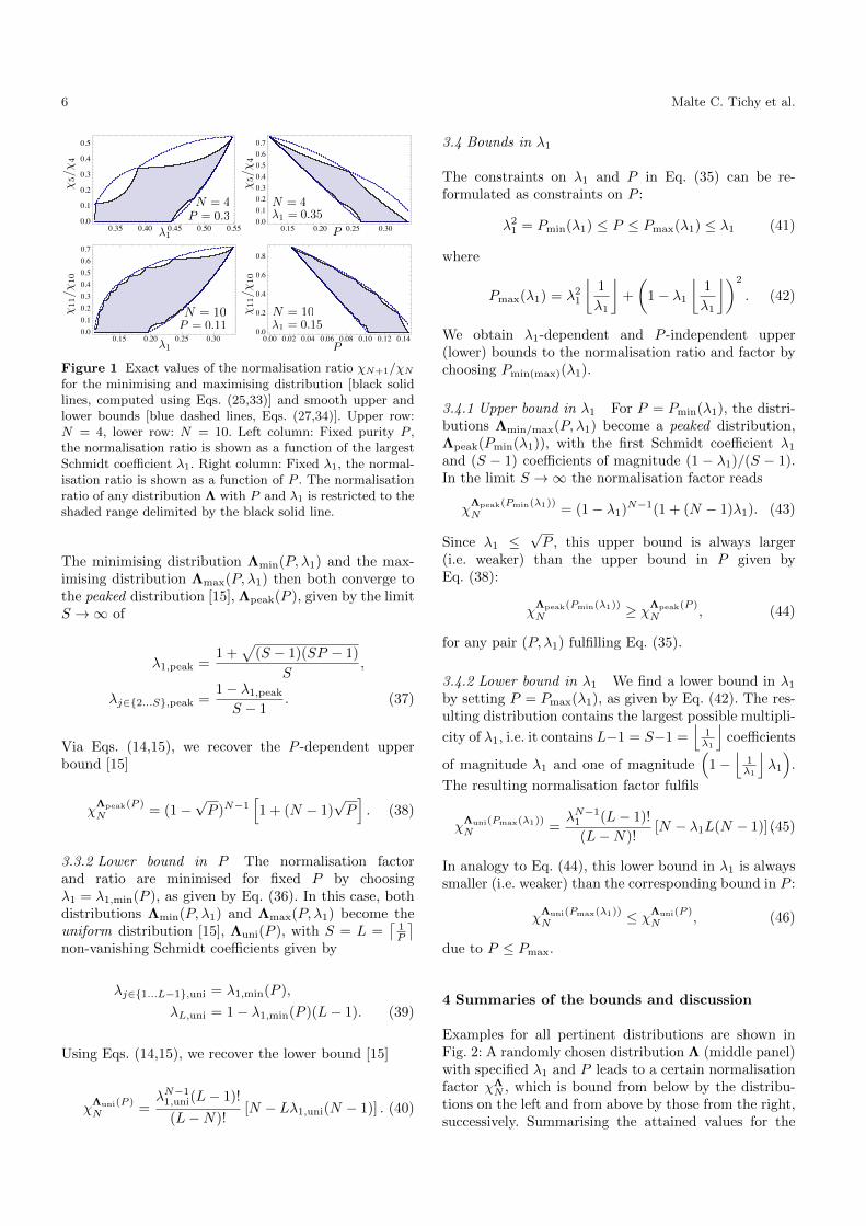
We compare the tight saturable bounds, Eqs. (25)and (33), with their respective smooth approximations,Eqs. (27) and (34), in Fig. 1.

3.3 Bounds in P

The parameters λ1 and P cannot be chosen independ-ently, since, by construction [22],

P ≤ λ1,min(P ) ≤ λ1 ≤ λ1,max(P ) =√P , (35)

where

λ1,min(P ) =1⌈1P

⌉ (√P⌈

1P

⌉− 1⌈

1P

⌉− 1

+ 1

). (36)

We obtain P -dependent and λ1-independent upper(lower) bounds to χN and χN+1/χN by fixing P andsetting the largest Schmidt coefficient to its extremalvalue, λ1,max(min)(P ).

3.3.1 Upper bound in P We maximise the normalisa-tion factor and ratio by choosing λ1 = λ1,max(P ) =

√P .

6 Malte C. Tichy et al.

P = 0.11

P = 0.3

1 = 0.15

1 = 0.35

1

1 P

P

11/

10

11/

10

5/

4

5/

4

N = 4 N = 4

N = 10N = 10

0.15 0.20 0.25 0.300.00.10.20.30.40.50.60.7

0.00 0.02 0.04 0.06 0.08 0.10 0.12 0.140.0

0.2

0.4

0.6

0.8

0.15 0.20 0.25 0.300.00.10.20.30.40.50.60.7

0.35 0.40 0.45 0.50 0.550.0

0.1

0.2

0.3

0.4

0.5

Figure 1 Exact values of the normalisation ratio χN+1/χN

for the minimising and maximising distribution [black solidlines, computed using Eqs. (25,33)] and smooth upper andlower bounds [blue dashed lines, Eqs. (27,34)]. Upper row:N = 4, lower row: N = 10. Left column: Fixed purity P ,the normalisation ratio is shown as a function of the largestSchmidt coefficient λ1. Right column: Fixed λ1, the normal-isation ratio is shown as a function of P . The normalisationratio of any distribution Λ with P and λ1 is restricted to theshaded range delimited by the black solid line.

The minimising distribution Λmin(P, λ1) and the max-imising distribution Λmax(P, λ1) then both converge tothe peaked distribution [15], Λpeak(P ), given by the limitS →∞ of

λ1,peak =1 +

√(S − 1)(SP − 1)

S,

λj∈2...S,peak =1− λ1,peakS − 1

. (37)

Via Eqs. (14,15), we recover the P -dependent upperbound [15]

χΛpeak(P )N = (1−

√P )N−1

[1 + (N − 1)

√P]. (38)

3.3.2 Lower bound in P The normalisation factorand ratio are minimised for fixed P by choosingλ1 = λ1,min(P ), as given by Eq. (36). In this case, bothdistributions Λmin(P, λ1) and Λmax(P, λ1) become theuniform distribution [15], Λuni(P ), with S = L =

⌈1P

⌉non-vanishing Schmidt coefficients given by

λj∈1...L−1,uni = λ1,min(P ),

λL,uni = 1− λ1,min(P )(L− 1). (39)

Using Eqs. (14,15), we recover the lower bound [15]

χΛuni(P )N =

λN−11,uni(L− 1)!

(L−N)![N − Lλ1,uni(N − 1)] . (40)

3.4 Bounds in λ1

The constraints on λ1 and P in Eq. (35) can be re-formulated as constraints on P :

λ21 = Pmin(λ1) ≤ P ≤ Pmax(λ1) ≤ λ1 (41)

where

Pmax(λ1) = λ21

⌊1

λ1

⌋+

(1− λ1

⌊1

λ1

⌋)2

. (42)

We obtain λ1-dependent and P -independent upper(lower) bounds to the normalisation ratio and factor bychoosing Pmin(max)(λ1).

3.4.1 Upper bound in λ1 For P = Pmin(λ1), the distri-butions Λmin/max(P, λ1) become a peaked distribution,Λpeak(Pmin(λ1)), with the first Schmidt coefficient λ1and (S − 1) coefficients of magnitude (1 − λ1)/(S − 1).In the limit S →∞ the normalisation factor reads

χΛpeak(Pmin(λ1))N = (1− λ1)N−1(1 + (N − 1)λ1). (43)

Since λ1 ≤√P , this upper bound is always larger

(i.e. weaker) than the upper bound in P given byEq. (38):

χΛpeak(Pmin(λ1))N ≥ χΛpeak(P )

N , (44)

for any pair (P, λ1) fulfilling Eq. (35).

3.4.2 Lower bound in λ1 We find a lower bound in λ1by setting P = Pmax(λ1), as given by Eq. (42). The res-ulting distribution contains the largest possible multipli-

city of λ1, i.e. it contains L−1 = S−1 =⌊

1λ1

⌋coefficients

of magnitude λ1 and one of magnitude(

1−⌊

1λ1

⌋λ1

).

The resulting normalisation factor fulfils

χΛuni(Pmax(λ1))N =

λN−11 (L− 1)!

(L−N)![N − λ1L(N − 1)] .(45)

In analogy to Eq. (44), this lower bound in λ1 is alwayssmaller (i.e. weaker) than the corresponding bound in P :

χΛuni(Pmax(λ1))N ≤ χΛuni(P )

N , (46)

due to P ≤ Pmax.

4 Summaries of the bounds and discussion

Examples for all pertinent distributions are shown inFig. 2: A randomly chosen distribution Λ (middle panel)with specified λ1 and P leads to a certain normalisationfactor χΛ

N , which is bound from below by the distribu-tions on the left and from above by those from the right,successively. Summarising the attained values for the

How bosonic is a pair of fermions? 7

uni(Pmax(1)) uni(P ) min(1, P ) max(1, P ) peak(P ) peak(Pmin(1))

Figure 2 Hierarchy of minimising and maximising distributions. The circle diameters correspond to the magnitude of aSchmidt coefficient λj , and the fraction of filled area in each large circle is the purity P of the respective distribution. Adistribution Λ, with λ1 = 0.3 and P = 0.2 (center) leads to a normalisation factor χN that is bound from below and fromabove by the χN evaluated for the distributions on the left and on the right, respectively. The order of the distributionsreflects the hierarchy of Eq. (47). All circles that correspond to λ1 are filled with dark red and marked with white arrows.The resulting normalisation ratios χN+1/χN obey the same hierarchy, as illustrated by the intersections of the vertical lines(i) with the three minimising and the three maximising limits in Fig. 3. The normalisation ratio of Λ then lies on (i) withinthe shaded area.

normalisation factor given in Eqs. (25,33,38,40,43,45),we obtain our main result,

χΛuni(Pmax(λ1))N ≤ χΛuni(P )

N ≤ χΛmin(λ1,P )N

≤ χΛN ≤ (47)

χΛmax(λ1,P )N ≤ χΛpeak(P )

N ≤ χΛpeak(Pmin(λ1))N .

This hierarchy of consecutively tighter bounds is imme-diately inherited by the normalisation ratio χN+1/χNin full analogy, which quantitatively answers our initialquestion, “How bosonic is a pair of fermions?”, in termsof P and λ1.

In order to obtain a physical understanding of thesebounds, a combinatorial approach is instructive: Thenormalisation factor χN can be interpreted as the prob-ability that a collection of N objects that are each givena property j with probability λj does not contain any setof two or more objects with the same property [23] (forS = 365 and λj = 1/365, we recover the “birthday prob-lem” [31]). In our physical context, no two or more bi-fermions are allowed to occupy the same Schmidt mode.The Pauli principle, enforced by Eq. (6), enforces thatthe emerging N -coboson state in Eq. (8) does not con-tain any such terms describing multiple occupation. Thelack of these terms then needs to be accounted for bythe normalisation factor χN .

4.1 Entanglement and bosonic behavior

Combinatorially speaking, the purity P represents theprobability that two randomly chosen objects possessthe same property (it is therefore also called the colli-sion entropy). Here, it reflects the probability that thewavefunction vanishes upon two bi-fermions competingfor the same Schmidt mode. Therefore, the P -dependentbounds on χN decrease monotonically with increasingP (blue dotted lines in the right panels of Fig. 3). Lar-ger entanglement, characterised by a smaller purity P ,

31/

30

P = 0.02

N = 30

d

4/

31

1,max(P )1,min(P )

1

P = 0.2

N = 3

dPmax(1)Pmin(1)

1 = 0.3

N = 3

d

1 = 0.03

N = 30

d

31/

30

4/

3

P

P0 0.01 0.02 0.03

0.0

0.2

0.4

0.6

0.8

1.00.0009 0.0298

0.0

0.2

0.4

0.6

0.8

1.0

0.09 0.280.0

0.2

0.4

0.6

0.8

1.00 0.1 0.2 0.3

0.0

0.2

0.4

0.6

0.8

1.0

0.2 0.4472140.0

0.2

0.4

0.6

0.8

1.00 0.1 0.2 0.3 0.4 0.5

0 0.05 0.1 0.150.0

0.2

0.4

0.6

0.8

1.00.02 0.141421

(a)

(b)(i) (i)

(ii)(ii)

Figure 3 Upper and lower bounds to the normalisation ra-tio χN+1/χN as a function of λ1 (left panels) and P (rightpanels), for N = 3 (top row) and N = 30 (bottom row). Reddashed lines correspond to bounds in λ1 alone, Eqs. (43,45);blue dotted lines show the bounds in P alone, Eq. (38,40).The combined bounds, Eqs. (25,33), are shown as solid blacklines, the shaded area is the range allowed for general distri-butions Λ with given λ1 and P . The bounds in P are alwayssuperior to those in λ1. By setting P (left panel) or λ1 (rightpanel), the possible values of λ1 and P , respectively, are con-strained by Eqs. (35) and (41). The solid vertical lines in theupper panels indicate those values for which the maximisingand minimising distributions are depicted in Fig. 2 [solid redlines (i), λ1 = 0.3, P = 0.2] and Fig. 4 [solid dark blue lines,P = 0.2, (a) λ1 = 0.215, (b) λ1 = 0.42]. The vertical lines(ii) in the lower panel indicate corresponding values of P andλ1.

is therefore tantamount to a more bosonic composite[3, 12, 23].

Similarly, the λ1-dependent bounds decrease with in-creasing λ1 (red dashed lines in the left panel of Fig. 3).Consistently, an increase of λ1 also leads to weaker geo-metric entanglement, EG = 1− λ21. This connection un-derlines, again, the relationship between quantum en-tanglement and the bosonic behavior of composites.

8 Malte C. Tichy et al.

The knowledge of λ1 alone leaves a finite rangefor possible values of P [see Eq. (41)]: The remaining,unknown Schmidt coefficients λ2 . . . λS may be manyand small, or few and large (compare the distributionΛuni(Pmax(λ1)) to Λpeak(Pmin(λ1)) in Fig. 2). Indeed,the main sources of deviation from bosonic behavior arebinary “collisions” of bi-fermions, which is directly quan-tified by P . Therefore, bounds in λ1 are always weakerthan bounds in P ; in the formalism of quantum informa-tion, the purity P is more decisive than the overlap withthe closest separable state, λ1.

The knowledge of both, λ1 and P , yields a consider-able enhancement over bounds in P alone (black solidlines in Fig. 3). In particular, the range of possible χNbecomes narrower for extremal values of P or λ1, forwhich the minimising and maximising distributions re-semble each other, as in Fig. 4. In this case, λ1 and Pstrongly constrain the remaining Schmidt coefficients.

In view of the clear dependence of χN on P andλ1, it is remarkable that the combined bound in P andλ1 features an increase of the bosonic quality χN andχN+1/χN with λ1 (Fig. 3). This increase, however, is dueto the fixed purity P : By increasing the largest Schmidtcoefficient λ1, all other Schmidt coefficients need to de-crease in order to keep P constant, which naturally in-creases the total accessible number of Schmidt modes,and, consequently, χN . More formally speaking, χN ac-tually increases with M(3), as can be inferred fromEqs. (11,13) [13].

4.2 Limit of large coboson numbers N

In Fig. 5, we show the deviation from the ideal valueχN+1/χN = 1 as a function of the number of cobosonsN . While the upper and lower bounds in P convergefor small values of N < 1/

√P , bounds in λ1 do not:

For small particle numbers, the coboson behaviour isessentially defined by the binary collision probability, i.e.by the purity P . The magnitude of the largest Schmidtcoefficient λ1 is secondary. For large particle numbersN > 1/

√P , the knowledge of λ1 then fixes the possible

range of M(3), which constrains the accessible values ofthe normalisation ratio. Again, very large or very smallvalues of λ1 lead to a tighter confinement of the range ofpossible χN+1/χN than intermediate values of λ1, as canbe seen by comparing the panels in Fig. 5. In general, λ1and P determine to a wide extent up to which numberof cobosons N a condensate of two-fermion compositesstill behaves bosonically [6, 32].

In comparison to the bounds on the normalisationfactor for cobosons made of two elementary bosons [22],the role of the λ1-dependent bounds is exchanged: fortwo-fermion cobosons, χN is maximised (minimised) bychoosing the smallest (largest) possible purity for a givenλ1; for two-boson cobosons, the normalisation factor in-stead increases with the purity. As a consequence, the

clear hierarchy of bounds expressed by Eq. (47) is absentfor two-boson cobosons [22]. This dependence is due tothe possibility for multiple occupation of Schmidt modesby bosonic constituents, forbidden by the Pauli principlefor fermionic constituents. Furthermore, when the num-ber of cobosons N is large, N > 1/λ1, the behaviour oftwo-boson bosons is very well defined by λ1 alone, andthe multiple occupation of the most prominent Schmidtmode dominates the picture, a process without analogyin the present two-fermion case.

(a) (b)

1 = 0.215 1 = 0.42

min max min max

Figure 4 Minimising and maximising distributionsΛmin/max, for close-to-extremal values of λ1 andfixed P = 0.2. (a) λ1 = 0.215 ' λ1,min(P ). (b)λ1 = 0.42 / λ1,max(P ). The emerging bounds correspond tothe black solid lines in Fig. 3 at the intersections with arrows(a) and (b), respectively. For λ1 → λ1,max(min)(P ), thedistributions converge to the peaked (uniform) distribution(compare to the corresponding sketches in Fig. 2).

Particle number N

(a) (b)

(c) (d)

Dev

iati

on

from

idea

lboso

ns

(1

N+

1/

N)

Dev

iati

on

from

idea

lboso

ns

(1

N+

1/

N)

1 10 100 1000 104

10-4

0.001

0.01

0.1

11 10 100 1000 104

10-4

0.001

0.01

0.1

1

1 10 100 1000 104

0.001

0.01

0.1

11 10 100 1000 104

0.001

0.01

0.1

1

1 10 100 1000 1040.001

0.0050.010

0.0500.100

0.5001.000

1 10 100 1000 104

0.001

0.0050.010

0.0500.100

0.5001.000

1 10 100 1000 1040.001

0.0050.010

0.0500.100

0.5001.000

1 10 100 1000 104

0.001

0.0050.010

0.0500.100

0.5001.000

Figure 5 Upper and lower bounds to (1 − χN+1/χN ),i.e. to the deviation from ideal bosonic behaviour, as afunction of N . The color-code is the same as in Fig. 3. Inall panels, P = 0.001, i.e. the bounds in P alone (blue dot-ted) do not change. We choose different values of λ1:(a) λ1 = 0.9λ1,min(P ) + 0.1λ1,max(P ) ≈ 0.0041.(b) λ1 = 0.5λ1,min(P ) + 0.5λ1,max(P ) ≈ 0.0163.(c) λ1 = 0.1λ1,min(P ) + 0.9λ1,max(P ) ≈ 0.0286.(d) λ1 = 0.01λ1,min(P ) + 0.99λ1,max(P ) ≈ 0.0313.

How bosonic is a pair of fermions? 9

5 Conclusions and outlook

Starting with the general description of a two-fermioncomposite in Eqs. (1,4), we confined the quantitativeindicator χN+1/χN for the bosonic behaviour of theresulting coboson. For a fixed purity P , the immedi-ate difference between the state that minimises and thestate that maximises χN is the magnitude of the largestSchmidt coefficient, which is of the order of P for theminimal, uniform distribution, and

√P for the max-

imal, peaked distribution [23]. Therefore, the additionalconstraint on λ1 can considerably enhance P -dependentbounds [10, 12, 23].

Our bounds strengthen the relation betweenquantum entanglement and the bosonic quality of bi-fermion pairs, first established in Ref. [3]: Not only isthe purity P a quantitative indicator for bosonic be-havior [3, 12, 13, 23], but so is the geometric measureof entanglement [29], which can be expressed here as afunction of λ1.

Depending on the application, the single-fermionpurity P , the largest eigenvalue λ1 of the single-fermiondensity matrix ρ(a/b), or both may be known. We canformulate a clear hierarchy: Knowledge of P is morevaluable than the knowledge of λ1 alone, whereas thecombination can greatly enhance the bounds, depend-ing on the value of the involved parameters. The effectof compositeness are observable in any physical observ-able that is affected by the commutation relation (20),such as, e.g., bosonic signatures in multiparticle interfer-ence [15].

Our method can be extended to formulate evenstronger bounds that depend on the purity P and onthe m largest Schmidt coefficients λ1 ≥ λ2 ≥ · · · ≥ λm:In close analogy to the procedure in Appendix A andB, minimising and maximising distributions can be con-structed, and the resulting normalisation factors can becomputed. The increased accuracy will, however, comeat the expense of an increased computational cost, sincea larger number of distinct Schmidt coefficients (up tom + 2 when we fix the m largest coefficients and thepurity P ) also leads to a larger number of sums whenEq. (15) is applied.

Another desideratum is the extension of the presentbounds to multi-fermion systems in order to character-ise, e.g., α-particles in extreme environments [33, 34].The absence of the Schmidt decomposition, Eq. (1), formultipartite states [4] makes this task, however, ratherchallenging. In particular, a simple combinatorial inter-pretation of the normalisation constant seems to be ex-cluded for such composites.

Acknowledgments

The authors would like to thank Florian Mintert, LukaszRudnicki, Alagu Thilagam and Nikolaj Th. Zinner for

stimulating discussions, and Christian K. Andersen,Durga Dasari, Jake Gulliksen, Pinja Haikka, David Pet-rosyan and Andrew C. J. Wade for valuable feedback onthe manuscript. M.C.T. gratefully acknowledges supportby the Alexander von Humboldt-Foundation through aFeodor Lynen Fellowship. K.M. gratefully acknowledgessupport by the Villum Foundation. P.A.B. gratefully ac-knowledges support by the Progama de Movilidad Inter-nacional CEI BioTic en el marco PAP-Erasmus.

A Appendix: Minimising distribution

A.1 Uniforming operation

In close analogy to the proofs for the bounds inRef. [23] and following an analysis of the birthday-problem with non-uniform birthday probabilities [31],we define a uniforming operation Γu on the distribu-tion Λ that can modify three selected λj with indices2 ≤ j1 < j2 < j3 ≤ S (i.e. the operation never acts onthe first Schmidt coefficient λ1, since its value is fixed,by assumption). We will show that this operation alwaysdecreases χN , and specify the distribution Λmin(P, λ1)that remains invariant under the application of Γu. Thisdistribution thus minimises χΛ

N under the constraints(P, λ1).

The operation Γu modifies three coefficients in a dis-tribution,

Γu : (λj1 , λj2 , λj3)→ (λuj1 , λuj2 , λ

uj3), (48)

such that it leaves

K1 = λj1 + λj2 + λj3 ,

K2 = λ2j1 + λ2j2 + λ2j3 , (49)

invariant, and, consequently, also∑j λj = 1 and∑

j λ2j = P . The third power-sum, M(3) =

∑j λ

3j , how-

ever, is changed by the application of Γu. Specifically,

λuj1 = λuj2 =1

6

(2K1 +

√6K2 − 2K2

1

),

λuj3 =1

3

(K1 −

√6K2 − 2K2

1

), (50)

For K21 < 2K2, we formally have λuj3 < 0, and we altern-

atively set

λuj1/j2 =1

2

(K1 ±

√2K2 −K2

1

), (51)

λuj3 = 0.

Colloquially speaking, Γu levels out the three coeffi-cients λj1 , λj2 , λj3 and thus makes the distribution moreuniform, while the purity P is kept constant.

10 Malte C. Tichy et al.

A.1.1 The product λj1λj2λj3 decreases under Γu Itholds

λuj1λuj2λ

uj3 ≤ λj1λj2λj3 . (52)

Proof: We write the left- and right-hand side of (52)in terms of K1,K2 and λj1

λuj1λuj2λ

uj3 =

=

1

108

(K1 −

√6K2 − 2K2

1

)×(

2K1 +√

6K2 − 2K21

)2for K2

1 > 2K2

0 for K21 ≤ 2K2

(53)

λj1λj2λj3 =1

2λj1(2λ2j1 − 2λj1K1 +K2

1 −K2

)For given K1 and K2, we can find the possible ori-

ginal λj2/j3 as a function of λj1 ,

λj2/j3 =1

2

(K1 − λj1 ±

√2λj1K1 −K2

1 − 3λ2j1 + 2K2

)The requirement λj1 ≥ λj2 ≥ λj3 ≥ 0 imposes

K1

3+

√3K2 −K2

1

3√

2≤ λj1 ≤

K1

3+

√6K2 − 2K2

1

3(54)

Given K1,K2, all allowed values of λj1 then fulfillEq. (52). ut

A.1.2 χΛN decreases upon application of Γu Upon ap-

plication of Γu, the normalisation constant χN and thenormalisation ratio χN+1/χN can only decrease:

χΓu(Λ)N ≤ χΛ

N , (55)

χΓu(Λ)N+1

χΓu(Λ)N

≤ χΛN+1

χΛN

. (56)

Proof: Without loss of generality and for convenienceof notation, we set j1 = 2, j2 = 3, j3 = 4, i.e. we letthe operations act on the first three non-fixed Schmidtcoefficients. We define

χN = χ(λ1,λ5,...,λS)N , (57)

i.e. formally χN is a normalisation factor, but for theunnormalised distribution (λ1, λ4, . . . , λS). We can thenwrite χN as

χN = λ2λ3λ4 · χN−3 + (λ2λ3 + λ4λ3 + λ2λ4)χN−2

+(λ2 + λ3 + λ4)χN−1 + χN . (58)

The terms

λ2λ3 + λ4λ3 + λ2λ4 =1

2

(K2

1 −K2

), (59)

λ2 + λ3 + λ4 = K1, (60)

and χk with k ∈ N − 3, . . . , N do not change uponapplication of Γu, i.e. only the product λ2λ3λ4 is af-fected by the operations. Eq. (52) then implies that χΛ

N

decreases upon the application of Γu.Using χN+1 ≤ χN , one can easily show in analogy

to Ref. [23] that the inequality (55) is inherited by thenormalisation ratio (56). ut

A.2 Properties of the minimising distribution

The distribution Λmin(P, λ1) that minimises χN for fixedλ1 and P should remain invariant under the applica-tion of Γu, for all choices of 2 ≤ j1, j2, j3 ≤ S. By thedefinition of Γu, we see that any three coefficients withλj1 > λj2 = λj3 never constitute a fixed point of Γu.Therefore, the invariant distribution is of the form

λ1 ≥ λ2 = · · · = λS−1 ≥ λS . (61)

It coincides with the distribution found in Ref. [22].

B Appendix: Maximising distribution

B.1 Peaking operation

With K1 and K2 defined as in Eq. (49) above, wedefine the peaking operation Γ p as follows: For K1 +√

6K2 − 2K21 ≤ 3λ1, we set

λpj1 =1

3

(K1 +

√6K2 − 2K2

1

),

λpj2 = λpj3 =1

6

(2K1 −

√6K2 − 2K2

1

). (62)

If K1 +√

6K2 − 2K21 > 3λ1, the above definition leads

to λpj1 > λ1, which we excluded by assumption. In thiscase, we define alternatively

λpj1 = λ1 (63)

λpj2/j3 =K1 − λ1 ±

√2(K2 − λ21)− (K1 − λ1)2

2,

for which λ1 = λpj1 ≥ λpj2 ≥ λpj3 ≥ 0. In full analogy tothe discussion in Sections A.1.1, A.1.2, one shows that

χΛN ≤ χΓ

p(Λ)N ,

χΛN+1

χΛN

≤ χΓp(Λ)N+1

χΓp(Λ)N

, (64)

i.e. the normalisation factor and ratio increase under theapplication of Γ p.

B.2 Properties of the maximising distribution

The distribution Λmax(P, λ1) that maximises χN forfixed λ1 and P is obtained as follows: We maximise themultiplicity of λ1 in Λ, i.e. λ1 is repeated L − 1 times,with L = dP/λ21e. The coefficients then need to fulfil

λ1 = · · · = λL−1 ≥ λL ≥ λL+1 = · · · = λS , (65)

to ensure that Λmax(P, λ1) be a fixed point of Γ p. Again,the distribution coincides with the one found in Ref. [22].

How bosonic is a pair of fermions? 11

References

1. ALICE Collaboration. Two-pion Bose-Einstein cor-relations in pp collisions at sqrt[s]=900 GeV. Phys.Rev. D, 82:052001, 2010.

2. M. Zwierlein, C. Stan, C. Schunck, S. Raupach,S. Gupta, Z. Hadzibabic, and W. Ketterle. Obser-vation of Bose-Einstein Condensation of Molecules.Phys. Rev. Lett., 91:250401, 2003.

3. C. K. Law. Quantum entanglement as an interpret-ation of bosonic character in composite two-particlesystems. Phys. Rev. A, 71:034306, 2005.

4. R. Horodecki, M. Horodecki, and K. Horodecki.Quantum entanglement. Rev. Mod. Phys., 81:865,2009.

5. M. C. Tichy, F. Mintert, and A. Buchleitner. Essen-tial entanglement for atomic and molecular physics.J. Phys. B: At. Mol. Opt. Phys., 44:192001, 2011.

6. S. Rombouts, D. V. Neck, K. Peirs, and L. Pollet.Maximum occupation number for composite bosonstates. Mod. Phys. Lett., A17:1899, 2002.

7. P. Sancho. Compositeness effects, Pauli’s principleand entanglement. J. Phys. A: Math. Theor., 39:12525, 2006.

8. A. Gavrilik and Y. A. Mishchenko. Entanglement incomposite bosons realized by deformed oscillators.Phys. Lett. A, 376:1596, 2012.

9. A. M. Gavrilik and Y. A. Mishchenko. Energy de-pendence of the entanglement entropy of compos-ite boson (quasiboson) systems. J. Phys. A: Math.Theor., 46:145301, 2013.

10. M. Combescot. “Commutator formalism” for pairscorrelated through Schmidt decomposition as usedin Quantum Information. Europhys. Lett., 96:60002,2011.

11. M. Combescot, X. Leyronas, and C. Tanguy. On theN-exciton normalization factor. Europ. Phys. J. B,31:17, 2003.

12. C. Chudzicki, O. Oke, and W. K. Wootters. Entan-glement and Composite Bosons. Phys. Rev. Lett.,104:070402, 2010.

13. R. Ramanathan, P. Kurzynski, T. Chuan, M. Santos,and D. Kaszlikowski. Criteria for two distinguishablefermions to form a boson. Phys. Rev. A, 84:034304,2011.

14. S. S. Avancini, J. R. Marinelli, and G. Krein. Com-positeness effects in the Bose-Einstein condensation.J. Phys. A: Math. Theor., 36:9045, 2003.

15. M. C. Tichy, P. A. Bouvrie, and K. Mølmer. Collect-ive Interference of Composite Two-Fermion Bosons.Phys. Rev. Lett., 109:260403, 2012.

16. P. Kurzynski, R. Ramanathan, A. Soeda, T. K.Chuan, and D. Kaszlikowski. Particle addition andsubtraction channels and the behavior of compositeparticles. New J. Phys., 14:093047, 2012.

17. S.-Y. Lee, J. Thompson, P. Kurzynski, A. Soeda,and D. Kaszlikowski. Coherent states of compositebosons. arXiv:1309.4847, 2013.

18. T. K. Chuan and D. Kaszlikowski. CompositeParticles and the Szilard Engine. arxiv:1308.1525,2013.

19. T. Brougham, S. M. Barnett, and I. Jex. Interferenceof composite bosons. J. Mod. Opt., 57:587, 2010.

20. M. Combescot, F. Dubin, and M. Dupertuis. Role ofFermion Exchanges in Statistical Signatures of Com-posite Bosons. Phys. Rev. A, 80:013612, 2009.

21. A. Thilagam. Binding energies of composite bosonclusters using the Szilard engine. arXiv:1309.6493,2013.

22. M. C. Tichy, P. A. Bouvrie, and K. Mølmer. Bo-sons made of bosons: Condensation of the whole orcondensation of the parts? arXiv:1308.2896, 2013.

23. M. C. Tichy, P. A. Bouvrie, and K. Mølmer. Bosonicbehavior of entangled fermions. Phys. Rev. A, 86:042317, 2012.

24. D. Bernstein. Matrix Mathematics: Theory, Facts,and Formulas. Princeton University Press, Prin-ceton, 2009.

25. M. Combescot, O. Betbeder-Matibet, and F. Dubin.The many-body physics of composite bosons. Phys.Rep., 463:215, 2008.

26. I. G. Macdonald. Symmetric Functions and HallPolynomials. Clarendon Press, Oxford, 1995.

27. A. Thilagam. Crossover from bosonic to fermi-onic features in composite boson systems. J. Math.Chem., 51:1897, 2013.

28. R. Grobe, K. Rzazewski, and J. H. Eberly. Measureof electron-electron correlation in atomic physics. J.Phys. B: At. Mol. Opt. Phys., 27:L503, 1994.

29. T.-C. Wei and P. M. Goldbart. Geometric meas-ure of entanglement and applications to bipartiteand multipartite quantum states. Phys. Rev. A, 68:042307, 2003.

30. F. W. J. Olver, D. W. Lozier, R. F. Boisvert, andC. W. Clark, editors. NIST Handbook of Mathem-atical Functions. Cambridge University Press, NewYork, NY, 2010.

31. A. G. Munford. A note on the uniformity assump-tion in the birthday problem. Amer. Statist., 31:119,1977.

32. M. Combescot and D. Snoke. Stability of a Bose-Einstein condensate revisited for composite bosons.Phys. Rev. B, 78:144303, 2008.

33. N. Zinner and A. Jensen. Nuclear α-particle con-densates: Definitions, occurrence conditions, andconsequences. Phys. Rev. C, 78:041306, 2008.

34. Y. Funaki, H. Horiuchi, W. von Oertzen, G. Ropke,P. Schuck, A. Tohsaki, and T. Yamada. Concepts ofnuclear α-particle condensation. Phys. Rev. C, 80:064326, 2009.