J . Fluid Mech. (1990), vol. 213, p p . 531-547 PrintPd in Great Brihin,

53 1

The vibrating ribbon problem revisited

By DAVID E. ASHPIS’ A N D ELI RESHOTKO’ ’NASA Lewis Research Center, Cleveland, OH 44135, USA

Department of Mechanid and Aerospace Engineering, Case Western Reserve University, Cleveland, OH 44106, USA

(Received 3 January 1989 and in revised form 29 September 1989)

A revised formal solution of the vibrating ribbon problem of hydrodynamic stability is presented. The initial formulation of Gaster (1965) is modified by application of the Briggs method and a careful treatment of the complex double Fourier transform inversions. Expressions are obtained in a natural way for the discrete spectrum as well as for the four branches of the continuous spectra. These correspond to discrete and branch-cut singularities in the complex wavenumber plane. The solutions from the continuous spectra decay both upstream and downstream of the ribbon, with the decay in the upstream direction being much more rapid than that in the downstream direction. Comments and clarification of related prior work are made.

1. Introduction The vibrating ribbon became a common experimental device in hydrodynamic

stability research since its first use by Schubauer & Skramstad (1947) to excite Tollmien-Schlichting (TS) waves in boundary-layer flow. The importance of this fundamental device goes beyond this practical application. The vibrating ribbon problem serves as a simple example of receptivity problems, which express the effect of imposed disturbances on the flow, and are significant in describing the onset of instabilities leading to transition from laminar to turbulent flow.

This problem, also known as the signalling problem, was initially treated by Gaster (1965), whose analysis verified Schubauer & Skramstad’s observation that in the time-asymptotic (long-time) limit the ribbon excites the spatial eigenmodes of the flow a t its own frequency. Additional analytical work is reported in the Russian literature (e.g. Tumin & Fedorov 1984). In free shear layers the signalling problem was treated by Huerre & Monkewitz (1985) for the inviscid case. We found Gaster’s solution incomplete. Mainly missing are the continuous spectra. Therefore we provide here a corrected and complete solution.

Gaster’s initial formulation of the problem is followed : the model, the formulation as an initial boundary value problem, and the application of a double Fourier transform (or Laplace-Fourier transform), are essentially identical, but we proceed with a different solution procedure. We use the Briggs method (Briggs 1964) to obtain the time-asymptotic solution. Common for a long time in plasma physics (see the review by Bers 1983), this method was first used in fluid mechanics by Tam (1971, 1978). It became more established in this field following a large number of its applications in later years. For example it was used by Huerre & Monkewitz (1985), Ashpis & Reshotko (1985), Leib & Goldstein (1986), Pierrehumbert (1986), Monkewitz & Sohn (1986), Hultgren & Aggarwal (1987), Monkewitz (1988), Lin & Lian (1989), Yang & Zebib (1989), and was reviewed by Huerre (1987). The Briggs

532 D. E . Ashpis and E. Reshotko

method requires an accurate account of the singularities in the transformed planes which is performed here in a methodical way. As a result the continuous spectra are included in our solution, and various related topics arc illuminated.

The continuous spectra were addressed by Case (1960, 1961) and by Murdock & Stewartson (1977). A comprehensive treatment was given by Grosch & Salwen (1978) and Salwen & Grosch (1981), who extended the classical normal mode formulation. They identified the one branch of the continuous spectra in the temporal case, and the four branches in the spatial case, and pointed out a difficulty in the physical interpretation of two of the branches in the spatial case.

Continuous spectra were obtained also in formulations of linear stability problems as an initial value problem and an initial boundary value problem. When solved by Fourier or Laplace transform methods, the continuous spectra emerge from branch- cuts in the complex transformed planes. The temporal continuous spectrum was obtained by Gustavsson (1979) who formulated an initial value problem. His work was used by Salwen & Grosch (1981) to prove completeness of the temporal eigenfunction expansion. Tsuge & Rogler (1983) treated a forced problem formulated as an initial boundary value problem and obtained two branches of the spatial continuous spectra, but dismissed one of them as non-physical. There is an inconsistency in their solution, which yielded a branch-cut singularity in a region of the complex transformed plane that should be analytic. The same branches were obtained also by Aldoss (1982). A similar forced problem for compressible flow was also treated as an initial boundary value problem by Tumin & Fedorov (1983), who found seven branches of the spatial continuous spectra. They recognized the same inconsistency, and proposed a method to resolve it.

I n the solution presented here, the continuous spectra emerge in a natural way as part of the complete formal solution and the solution is mathematically consistent. The solution procedure is applicable to a wider class of problems, and clarifies the prior difficulties. A comparison with Gaster (1965) and comments about related topics are included in the discussion of $6.

The present work is based on work first presented by Ashpis & Reshotko (1985) and detailed in Ashpis & Reshotko (1986), hereinafter referred to as AR.

2. Formulation of the problem The physical problem is modelled as shown in figure 1. Two-dimensional

incompressible boundary-layer flow over a flat plate is assumed, and the ribbon is modelled as a line source of disturbances imbedded at the wall at the origin 0 of the Cartesian coordinates x, y. The longitudinal and normal velocity components are U and V , respectively, and the free-stream velocity is Urn. We are interested in the response of the boundary layer to two-dimensional harmonic excitation of the ribbon starting a t t = 0.

The assumption is that the vibrations of the ribbon are infinitesimally small, justifying use of linear stability theory. The velocity is split into basic (0, V ) and disturbed ( u , v ) parts, and the standard procedures of linear stability theory are applied. Assuming parallel flow, V = 0, U = O(y), the non-dimensional equation for the normal disturbance velocity w is

where R is the Reynolds number based on U , and on the displacement thickness a*,

The vibrating ribbon problem 533

profile flow E l I Dm

l i

0

\

1 'L Vibrating ribbon

imbedded in wall

FIGURE 1. Model of the vibrating ribbon problem.

l7 = d20(y)/dy2, V2 = a2/ax2 +a2/ay2, and v = v(y ; x, t ) . The independent variables are used in the order y ; x, t throughout this paper, for convenience.

The effect of the ribbon is formulated as a wall boundary condition on the normal velocity

v(0 ; x, t ) = cos wo t S(X) H ( t ) , (2a )

where w,, is the real frequency of the vibration of the ribbon, 6 is Dirac's Delta function, which expresses the modelling of the ribbon as a line disturbance, and H ( t ) is the unit step function, which indicates that the motion starts from rest a t t = 0. The second boundary condition a t the wall, from continuity, is

As y + m it is required that

We use the generalized double Fourier transform defined as

@( y ; a, w ) = JYm dt 1:' dx v(y ; x, t ) e-i(as-wt), (4)

where a is the complex wavenumber and w is the complex frequeficy. The lower limit of the time integration can be replaced by 0, because v is a causal function in t . The Fourier transform on time is then equivalent to the Laplace transform on time, therefore (4) may also be referred to as a Laplace-Fourier transform.

Transforming ( 1 ) yields the Orr-Sommerfeld equation

{ (D2-a2) (D2-,i2)+itcRU'}{@} = 0, where

@ is considered a function of y, with a and w as parameters. R is also a parameter,

534 D. E . Ashpis and E. Reshotko

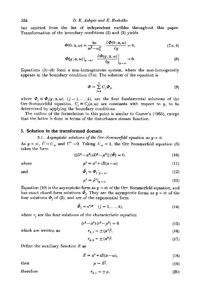
but omitted from the list of independent varibles throughout this paper. Transformation of the boundary conditions (2) and (3) yields

Equations (5)-(8) form a non-homogeneous system, where the non-homogeneity appears in the boundary condition (7a) . The solution of the equation is

where cBj = O j ( y ; a, w ) , ( j = 1, . . . ,4 ) , are the four fundamental solutions of the Orr-Sommerfeld equation. Ci = Cj(a, w ) are constants with respect to y , to be determined by applying the boundary conditions.

The outline of the formulation to this point is similar to Gaster’s (1965), except that the latter is done in terms of the disturbance stream function.

3. Solution in the transformed domain 3.1. Asymptotic solutions of the Orr-Sommerfeld equation as y -+ co

As y+ co, l7+ U, and P+O. Taking U , = 1, the Orr-Sommerfeld equation (5) takes the form

( (02- a21 (0’ -yz))> {6> = 0, (10)

where p2 = a2+iR(a-w) (11)

and @j = @jIu+,, (12)

(13)

Equation (10) is the asymptotic form as y -+ 00 of the Orr-Sommerfeld equation, and has exact closed-form solutions 6,. They are the asymptotic forms as y+ co of the four solutions Qi of ( 5 ) , and are of the exponential form

2 - ‘2 P - P ly-m

- cDj=erP (j= 1, ..., 4), (14)

where ri are the four solutions of the characteristic equation

( r 2 - a 2 ) ( T ~ - , $ ) = 0

which are written as r3, = f (pL2)i,

r4,2 = (a”;.

Define the auxiliary function Z as

The vibrating ribbon problem

(b)

2-plane

I1 iz'l I

BranchJ' cut

Z = [a2+iR(a-o)]

535

(4 p-plane

FIGURE 2. The mapping from the a-plane to the p-plane via the auxiliary plane 2. The hyperbolas a, and a, are mapped into 2, = 0, the hyperbolas b, and b, are mapped into 2, = 0. The (+ ) and (-) indicate the two sides of the branch-cut. Roman numerals indicate the quadrants of the Z- plane and their images in the p- and a-planes.

where p is the single-valued function obtained by taking the branch-cut along the negative real Z-axis and choosing the branch of p such that

Re@) > 0 for all 2. (21)

This convention for the complex square-root function is used throughout this paper. The function p depends on the three parameters a, w , and R. At fixed w and R , p

is viewed as a mapping of the a-plane to the p-plane via the auxiliary plane Z (figure 2). The two hyperbola sections a,,, in the p-plane are mapped to the branch-cut in the 2-plane, and therefore ensure that

Re@) > 0 for all a and w . (22 )

The coordinates of the branch-points BP,,, and the equations of the branch-cuts are given in AR. The branch-cuts for w with w, < 0 (we use the subscripts r and i to designate the real and imaginary parts throughout the paper) are symmetric with respect to the imaginary a-axis to the ones for w, > 0. In the w-plane, at fixed a and R, the branch-cut for p is a straight-line section (figure 3 a ) , similarly ensuring (22) . The coordinates of BP, are given in AR. This branch-cut for a with a, < 0 is symmetric with respect to the imaginary w-axis to the one for a, > 0.

For the evaluation of r4,p define the auxiliary function z

z = (a-iiE) (a+iiE), (23)

then let g = zi (24)

and thus r4, = f lim 5. E*O

536 D. E . Ashpie and E . Reshotko

w-Plane Fixed R a=(z = F %

analyticity 1

- w0

7 0'

a - p 1 an e Fixed R

w = w L

FIGURE 3. Undeflected contours for the inversion integrals (schematic). The points marked 0 in (a ) indicate poles for the a, marked 0 in (b). The curves passing through these points are trajectories w,(a,). Points marked x in (b) are poles for o marked x in (a). The curves passing through these points are trajectories a,(yL). The branch cut in (a) is for a = a,. The branch cuts in (b) are for w = wL. The question-marks in the left half-planes designate yet unknown existence of poles.

The branch-cuts which make 6 single valued are sections of the imaginary a-axis, from the branch-points +is to +im (figure 3 b ) , because they are mapped into the negative real z-axis, the branch-cut for (24). As s+O the branch-points approach the origin, and the branch-cuts span the whole imaginary a-axis, excluding the point of origin a = 0, which stays a regular point. By the choice of these branch-cuts it is ensured that

(26) Re([) > 0 for all a.

The asymptotic solutions are obtained by inserting r, from (20) and (25) into (14),

6,,3 = e+u, (27 a )

3.2. Application of the boundary conditions

Since y > 0, taking into account (22) and (26), it follows that and 6, are unbounded as y + 00, requiring C, = C, = 0. 6, and 6, decay as y+ co and are acceptable solutions. The constants C, and C, are determined by applying the boundary conditions (7) at the wall. The result for @ is

io A @ = @(y ;a ,o ) = --,

W 2 - W ; A o

The vibrating ribbon problem 537

where d E d ( y ; a , w ) = @l@;n-@;o@2, ( 2 9 4

do = d(0; a, w ) = @lo @;,,-CP;~ Qz0 (d at y = 0), (29b)

@* = @j(y; a, w ) ( j = 1 , 2 ) , (29 4 Gj0 E Qj(0; a, w ) ( j = 1 ,2 ) (CPj at y = 0), ( 2 9 4

d ( )’=-.

dY

It is important to emphasize the role of the particular choice of branch-cuts in this process. The solution would be more complicated if different branch-cuts had been constructed. Then the growth and decay of the solutions as y + 00 would depend on subdomains in the a- and w-planes. For example, with any branch-cuts other than au,d there will be a region D in the a-plane where m4 will be the decaying solution as y+ co. Then Q4 will be the acceptable solution in D , while will be the acceptable solution in the rest of the a-plane, requiring separate computations of the constants Cj and different expressions for @ in D and outside of it. With the present choice of branch-cuts, &8 decays as y+ co for all a and C, is always zero.

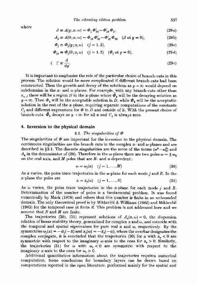
4. Inversion to the physical domain 4.1. The singularities of @

The singularities of @ are important for the inversion to the physical domain. The continuous singularities are the branch-cuts in the complex a- and w-planes and are described in $3.1. The discrete singularities are the zeros of the terms (w2-wi ) and A, in the denominator of (28) . Therefore in the w-plane there are two poles o = +wo on the real axis, and M poles that are R- and a-dependent :

w = w*(a) ( j = 1 , . . . , M ) (30)

As ar. varies, the poles trace trajectories in the w-plane for each mode j and R. In the a-plane the poles are

(31) a = a*(w) ( j = 1 , . . . ,N)

As w varies, the poles trace trajectories in the a-plane for each mode j and R. Determination of the number of poles is a fundamental problem. It was found numerically by Mack (1976) and others that this number is finite in an unbounded domain. The only theoretical proof is by MiklavEi6 & Williams (1982) and MiklavEiE (1983) for the temporal case at finite R. This problem is not addressed here and we assume that N and M are finite.

The trajectories (30), (31) represent solutions of do(a , o) = 0, the dispersion relation of linear stability theory, generalized for complex a and w , and coincide with the temporal and spatial eigenvalues for pure real a and o, respectively. By the symmetries wi(a) = -a,( - E ) and a j ( w ) = -aj( - a), where the overbar designates the complex conjugate, it is concluded that the trajectories (30) for a with a, < 0 are symmetric with respect to the imaginary waxis to the onea for a, > 0. Similarly, the trajectories (31) for w with w, < 0 are symmetric with respect to the imaginary u-axis to the ones for w, > 0.

Additional quantitative information about the trajectories requires numerical computation. Some conclusions for boundary layers can be drawn based on computations reported in the open literature, performed mainly for the spatial and

538 D . E . Ashpis and E . Reshotko

temporal formulations. These computations show that for finite R the number of eigenmodes N or M is finite, that for R > R,,, j = 1 is the only unstable mode (referred to herein as the unstable TS mode), and that the higher modes j = 2, . . . , N (or M ) are stable. When charted in the complex planes, the trajectories of the higher modes w,(a,) and a&) are in the lower half-w-plane and in the upper half-a-plane, respectively, for all R. At R > Re, the trajectory of the TS mode wI(ar) crosses the real w-axis and has a maximum in the upper half-w-plane, and the trajectory of a,(w,) crosses the real a-axis and has a minimum in the lower half-a-plane. The only reported computations for boundary layers known to us when both a and w are complex are by Gaster & Jordinson (1975) and Koch (1986). A limited range of trajectories for the TS mode a l ( w ) can be derived from thc data presented in those works. The trajectories provided by the latter work are, however, limited to negative values of wi, unfortunately a range that is not useful for the present analysis.

In addition, the existence of eigenvalues with negative real parts has never been reported in the literature. It is not clear if researchers have searched the left half- planes for eigenvalues without success, or if this search was not attempted at all. The implication for the present work is that the existence of trajectories (30) for a with a, > 0 in the left half-w-plane, and the existence of trajectories (31) for w with wr > 0 in the left half-a-plane, is unknown.

The comprehensive numerical computations required to obtain a complete picture of the trajectory maps are left for a separate work. Qualitative investigation, detailed in AR, shows that the constant wi trajectory of a l ( w ) shifts upward to above the real a-axis as wi is increased, which is partially verified by the results presented in Gaster & Jordinson (1975). Similar qualitative conclusions regarding the trajectories of the higher modes cannot be drawn based on the limited existing data. I n particular it is not known if trajectories can coalesce.

4.2. Inversion formula

Inversion of @ to the physical domain is obtained according to the inversion formula

where F and L are the inversion contours in the a- and the w-planes, respectively. They lie in the region of analyticity of 0 in each respective plane.

By properties of the Fourier transform of a function that is causal in t and defined for - co < x < 00, the regions of analyticity are an upper half-plane in the w-plane, and a strip that includes the real axis in the a-plane (figure 3). The strip is confined between +is. As s+O the strip degenerates to the real a-axis, allowed by the fact that the origin remains a regular point. Therefore F can be taken along the real a- axis, conveniently making a in (32) pure real.

The two inversions in (32) are interrelated. It means that if the w inversion is made first, a serves as a parameter whose value is taken along F . Since F coincides with the real a-axis, the singularities of interest in the w-plane are the ones for pure real a . The discrete ones are by definition the temporal eigenvalues, and the continuous ones are along the w defined by the straight-line branch-cut for a = ar, shown in figure 3(a). Since this branch-cut is always below the real w-axis (see AR), L lies in the upper half- w-plane above the maximum point of the temporal TS trajectory @,(a,) (ai = 0). If L is the line w = ic7, then c7 is positive, This conforms to the analyticity properties in the w-plane which were discussed above. If the a inversion is made first, the interdependence of the two inversions require the singularities in the a-plane to be

The vibmting ribbon problem

(4 iwi o-Plane

(b) a-Plane

R = const. > R,,

w = w, > 0 (w, = 0)

Upper iai t branch-cut 7 branch-cut

1

- r j = 1

(T-S mode)

539

FIGURE 4. (a ) Integration contour in the o-plane. (6) Closed integration contours in the a-plane. As w varies from 0 to x along the line w, = const. in (a), the poles a,(w) form the trajectories shown in (b). The hyperbola branch-cuts are shown for w, = 0.

18 FLM 213

540 D. E . Ashpis and E . Reshotko

taken for values of w on L, meaning for w with mi = (r. The previous discussion showed that for these w the poles are located in the upper half-a-plane, and in AR it is shown that the branch-cuts do not cross the real a-axis (the upper hyperbola branch-cut is above the real a-axis for wi > 0 and the lower hyperbola branch-cut stays below the real a-axis for all q), which conforms to the analyticity properties in the a-plane. At this point the inversion contours are determined and the inversion according to (32) can, a t least in principle, be performed.

4.3. The time-asymptotic form The present interest is principally in the time-asymptotic form of the solution, v as t -+ 00. For this purpose we apply the method of Briggs (Briggs 1964) (see fj 1). When using this mcthod, the inversion is made first from CL to x, to obtain 6 as

followed by inverting v” from w to t according to

The method of Briggs requires deflecting the contour L towards L,, which is located slightly below the real w-axis (figure 4 a ) . The exponential term in (34) will make the integrand vanish along the straight portions of L, as t +- co, leaving the time-asymptotic form to be determined by the singularities of v”(y;x,w) above L,. Simultaneously the contour F in the a-plane has to be deflected around constant-w, trajectories of a j ( w ) which cross the real a-axis as w i + 0 . The trajectory of the TS mode displays this behaviour, therefore F is deflected to F,, as shown in figure 4 ( 6 ) . The branch-cuts in the a-plane do not interfere with this process because, as explained in the previous section, the hyperbola branch-cuts do not cross the real a- axis (wi > 0 ) , and the imaginary axis branch-cuts do not depend on w a t all.

Finally, the Briggs method requires one to check the possibility of the coalescing of constant w, trajectories aj(o) originating a t opposite sides of the real a-axis. Such an occurrence yields a branch-cut of G in the w-plane which corresponds to an absolute instability if it is above the real w-axis. Investigation of this possibility requires knowledge of all the trajectories a j (w) . As discussed in $4.1 above, from spatial stability calculations it is only known that for wi = 0 all of the higher modes are above the real a-axis. The possibility that their trajectories move into the lower half-plane as wi is decreased from its value on L, and coalesce among themselves or with the trajectory of the TS mode, cannot be excluded a priori, and at present we make the assumption that coalescing of poles does not occur. The fact that absolute instabilities in boundary-layer flow were never observed experimentally supports this assumption. This assumption leads to the conclusion that v” has no branch-cut singularities above the real w-axis, and L can then be deflected to L, with the proper deflection of the contour around the poles T w o .

4.4. Inversion from a to x

First the inversion from a to x is performed according to

@(y; a, w ) eiaxda. (35)

The vibrating ribbon problem 54 1

To evaluate the integral we construct closed contours in the a-plane and apply the residue theorem. Two different contours are used, one for the domain x > 0, downstream of the ribbon, and the other for x < 0, upstream, as shown in figure 4 (b).

For x > 0 the contour is closed in the upper half-a-plane with the semicircle r, of radius r , deflected around the two branch-cuts. The closed contour consists of the section of Fl from - r to + r , of the sections of the semicircle r,, and of the four sides of the branch-cuts in the upper half-a-plane, marked as I: and II? (figure 4b). The residue theorem yields

N(U)

= 2ni C Res [@(y ; a, w ) eirrs]a-ap ( w ) , (36)

where the integrand has been omitted, and Nu) is the number of poles above Fl. The first integral represents integration along the section of Fl from --r to + r . The last four integrals represent integration around the branch-cuts, and the right-hand side is the sum over the residues a t the Nu) discrete poles a j ( w ) , designated with the superscript (u) .

For the domain x < 0 a similar semicircle r, is constructed in the lower half-a- plane, deflected around the branch-cuts there. Similar application of the residue theorem yields

.L + Jr,, + JI: + JI; + JII: + JII; j-1

$0

9-1 = -2ni 2 Res[@(y;a,w)ei“”],,,jl)(,,, (37)

where the sides Idf and IIf are the sides of the branch-cuts in the lower half-a-plane, as marked in figure 4(b), and the residues are calculated at the Nd) poles below Fl, designated with the superscript (4 ‘ ) .

As r - f 00 the first integral in the left-hand side of (36) and (37) approaches the integral in (35). The integrals on r, and r, for x > 0 and x < 0, respectively, are assumed to vanish as r + 00. The residues are computed with the assumption that all poles are of first order and the following result is obtained:

(38)

II: + Jr( + 11; + 11; + 111; + 111;

V (̂y; x, w ) = V ,̂(y; x, w ) + Gc(y; x, w ) ,

wherein 8, is the discrete spectrum in the w-plane, given as

aa where superscripts (u) and the upper sign are to be taken for the region x > 0, and the superscripts (4‘) and the lower sign are to be taken for x < 0. This notation is used hereafter. 8, are the continuous spectra

V^c(y; 2, w ) = 8c1(y; 5, w ) + 8c,(y; 2, w ) , (40)

where subscript 1 designates spectra originating from integration around the imaginary axis branch-cut, and 2 designates the spectra originating from the hyperbola branch-cuts as follows :

1 68 /)(y; x, w ) = - @(y ; a, w ) eiaz da - - 1 @(y ; a, w ) eias da, (41)

2n I; . (

1 B y ( y ; X , w ) = -- @(y; a, w ) eiaz da--/ @(y ; a, w ) eias da. (42)

2~ ‘s II:,t 2n I I ; , /

18-2

542 D. E . Ashpis and E . Reshotko

4.5. Inversion from w to t

Next 6 is inverted from w to t according to

w(y;z,t) = .G(y;x,w)e-i"tdw. I,, (43)

The integral vanishes on the straight section of L, for t -+ CO, leaving v to be calculated by integrating around the circles surrounding the poles fw,. Using the residue theorem,

v(y ; x, t ) = Res [v"(y; 2, w ) e-iwt]w=fwo. (44)

By observing (39), (41) and (42), it is seen that 4 consists of sums and integrals of functions of the form

(45) w a=- 2 9(y; X' @)-

W2-Wo

Using the symmetry property of g , g(y; x , w , ) = g(y;x, -0,)'

c Res = Re [9 (y ; x, w0)l. (46)

is obtained. Applying these results in (44) (see AR for detailed evaluation) leads to the final result for the time-asymptotic form of v as follows:

w(y; z, = "D(y; x, t , + v C ( y ; z, t ) ,

"c(Y; 5, t ) = %,(y ; 2, t ) + vc*(y ; x, t ) ,

(47 a )

(47 b )

where the various terms are detailed in the following. The superscripts (u) and (e) and the upper and lower signs are for the downstream (z > 0) and the upstream (z < 0) regions, respectively.

The discrete part of v, designated v,,, is

where the - designates that this is the time-asymptotic limit. A non-zero value for vD at z < 0 is contingent on the existence of poles in the left Half-plane as discussed before.

The continuous part of v originating from the imaginary-axis branch-cuts, designated vC,, is

where

wherein ia* = lim (e+icr). 6-0 +

The * signs correspond to the respective sides of the imaginary axis branch-cuts I:,( as shown in figure 4 ( b ) .

The vibrating ribbon problem 543

The continuous part of v originating from the hyperbola branch-cuts, designated

a;”,((a, wo), wo) 4; a&(@-, w ) (0 )

dO(a;Ju> wo), wo) do(a;Jg, wo), wo) - O ’ 0 1 , (52)

u is an integration variable, subscript a, designates the upper hyperbola branch-cut, a, the lower one, the superscripts designate the side of the respective branch-cut II$,[ as marked in figure 4 ( b ) .

cf, , and IT,,! are the coordinates of the branch-points aBP,,( = ( ~ 3 ~ , , k i u , , ~ ) for w = oo, and are given by the following equations:

For w,/R < 1 the following is obtained

(55 u-c)

5. Description of the results The expressions (48)-(54) show that the vibrating ribbon excites discrete and

continuous spectra, whose frequency in the time-asymptotic limit is equal to the frequency of the ribbon.

The discrete spectrum consists of the spatial eigenmodes of the flow. These are discrete travelling waves with frequency w, and wavenumber ajr (w0) . The phase velocity of the wave is

c . = wg (56) a&(%) 3

The growth factor is exp [ - a,i(wo) XI, and the coupling coefficient, indicating the extent to which the mode is excited, is

The quadrant in which the pole is located then determines the properties of its corresponding wave. Its region of influence is determined by its position above or below the contour Fl, The various possibilities are depicted in figure 5. Poles in the right half-a-plane correspond to waves propagating in the positive x-direction (positive phase velocity), and the ones in the left half-a-plane correspond to waves travelling in the negative x-direction. Growth in the region x > 0, downstream of the

544 D. E. Ashpis and E. Reshotko

(b i) x > o

(b ii) x < o

(b) Second quadrant

ujr < 0, aji > 0

cj+ I

(c ii)

x < o

x > o

(c) Third quadrant

a,r < 0, < 0

(a ii) x < o

(a) First quadrant

ajr > 0, aji > 0

(dii)

I x < o

x > o

(d) Fourth quadrant

FIGURE 5. Effects of the location of the pole in the a-plane on its corresponding wave for w, > 0 ; x , the aj for w, = 0; 0, aj for w = wL.

The vibrating ribbon problem 545

ribbon, is if the corresponding pole is below the real a-axis; and in the upstream region, x < 0, growth in the negative x-direction is if the pole is above the real a-axis. The right half-a-plane was thoroughly investigated numerically by various researchers (see discussion in $4 above), and the cases described in figure 5(aii) and (di) were not found.

For x+ 00, the higher &odes decay spatially, leaving the TS mode to be the dominant mode in the downstream region, and the summation in (48) for v,, (at x > 0) can be omitted.

The continuous spectra affect the regions upstream and downstream of the ribbon. In each region they consist of two parts; the one described by (49), consisting of a superposition of standing waves, and the one given by (51), which is a superposition of travelling waves. Some growth is possible in principle for finite x close to the origin; however, in both cases the waves decay away from the ribbon as x + k GO.

6. Discussion In the work presented here we have revisited the vibrating ribbon problem which

was first done by Gaster (1965). We have written the equations and the boundary conditions in terms of the disturbance normal velocity, while Gaster used the disturbance stream function. The two formulations are equivalent and lead to the same equation and boundary conditions. Except for this minor difference, we followed the formulation of Gaster up to the point where the double transform is applied (equation (9)). From there on our solution method differs considerably. We expressed the solution in terms of the fundamental solutions of the Orr-Sommerfeld equation, exercised some care in the evaluation procedure, and applied the Briggs method to obtain the time-asymptotic solution. The discrete spectrum obtained in the present work is equivalent to the one in Gaster, with the exception of a numerical error which is here corrected.

A significant outcome of the present work is that the solution includes the continuous spectra, which are missing from Gaster. The wave components of these spectra are identical to the spatial continuous spectra first obtained by Grosch & Salwen (1978) and Salwen & Grosch (1981) by looking for pure oscillatory eigenmodes of the Orr-Sommerfeld equation. Here these eigcnmodes emerge in a natural way, simply by constructing branch-cuts in the complex planes, as required whenever a complex square-root function is encountered.

It is here obtained that the ribbon has a downstream influence by excitation of both the discrete and continuous spectra. The new finding is that it also has an upstream influence via the continuous spectra. It is shown that the possibility of an additional upstream influence by excitation of the discrete spectra also needs to be considered. This can be verified or excluded only by a numerical search for poles in the left. half-plane, which correspond to spatial eigenvalues with negative real parts for positive frequencies (poles in the right half-a-plane with upstream influence, shown as cases (di) and (aii) in figure 5 were never found, as explained in $4.1). The spatial decay in the time-asymptotic limit of the continuous spectra is much greater in the upstream direction compared to the downstream direction. This is concluded from (55), showing that a t large Reynolds numbers (T( B ( T ~ , which affects the exponential decay terms preceding the integrals in (51).

The distinction between singularities affecting the upstream region and the ones affecting the downstream region is useful also in clarifying the difficulty expressed in Salwen & Grosch (1981). They point out that the wave component of the continuous

546 D. E . Ashpis and E . Reshotko

spectra which propagates upstream from x = CQ and the standing waves whose amplitudes increase towards x = co are not physically acceptable. This difficulty is resolved by the analysis here, which shows that these waves are excited only in the region upstream of the ribbon and therefore are physically acceptable.

Once solved systematically and correctly, the complex a- and w-planes contain all the discrete and continuous singularities, and the solution can serve as proof of completeness of the eigenfunction expansion in the spatial case. This is analogous to t,he proof of completeness for the temporal case done by Salwen & Grosch (1981) by comparing to the solution of Gustavsson (1979). Proof of completeness for this case is reported in an abstract by Salwen, Kelly & Grosch (1980), but details were never published.

Our solution also sheds light on the difficulties in the initial boundary value problem solutions reviewed in § 1. In these solutions a Laplace transform was applied to the longitudinal spatial coordinate x, which is equivalent to the Fourier transform of a function causal in x (a 90' rotation relates the Laplace S-plane to the Fourier a- plane). Therefore, formally, the application of the Laplace transform should yield the same discrete and continuous singularities as the Fourier transform. However, the complex S-planes in the work of Tsuge & Rogler (1983) and of Aldoss (1982) do not include the counterparts of the imaginary-axis branch-cuts. In addition there is an inconsistency in these works, as well as in Tumin & Fedorov (1983), where hranch- cut singularities protrude into what should be a half-plane of analyticity of the S- plane. As shown here, the disturbance introduced by the vibrating ribbon has an upstream influence, at least through the continuous spectra, and so will any disturbance introduced a t x = 0. By applying the Laplace transform this possibility is excluded, and i t is suggested that this is the source of the mathematical inconsistency, and that it is incorrect to use the Laplace transform in these problems.

This work was supported principally by the US Air Force Office of Scientific Research. The present paper was completed after the first author joined the NASA Lewis Research Center. The authors wish to thank the editor and the reviewers for t,heir useful comments.

R E F E R E N C E S

ALDOSS, T. K. 1982 Initial value study of effects of distributed roughness on boundary layer transition. Ph.D. dissertation, Case Western Reserve University.

ASHPIS, D. & RESHOTKO, E. 1985 The vibrating ribbon problem ~ revisited. Hull. AWL. Phgs. Soc. 30, 1708.

ASIIPIS, D. & RESHOTKO, E. 1986 On the application of Fourier transforms to the linear stability analysis of boundary layers. Case Western Reserve University Rep. FTAS/TR-86- 187. (Also Ashpis, D. E.. Ph.D. dissertation, Case Western Reserve University, 1986).

BERS, A. 1983 Space-time evolution of plasma instabilities - absolute and convective. In Basic Plasma Physica I (ed. A. A. Galeev & R. N. Sudan), pp. 451-517, Korth-Holland.

BRIGGS, R. J. 1964 Electron-Stream Interaction with Plasmas. MIT Press. CASE, K. M. 1960 Stability of inviscid plane Couette flow. Phys. Fluids 3, 143-158. CASE, K. M. 1961 Hydrodynamic stability and the inviscid limit. J . Fluid Mech. 10, 42&429. GASTER, M. 1965 On the generation of spatially growing waves in a boundary layer. J Fluid Mech.

GASTER, M. & JORDINSON, R. 1975 On the eigenvalues of the Orr-Sommerfeld equation. J Fluid

GROSCH, C. E. & SALWEN, H. 1978 The continuous spectrum of the Orr-Sommerfeld equation.

22, 433441.

Mech. 72, 121-133.

Part 1 . The spectrum and the eigenfunctions. J . Fluid Mrch 87, 33-54.

The vibrating ribbon problem 547

GUSTAVSSON, L. H . 1979 Initial-value problem for boundary layer flows. Phys. Fluids 22,

HUERRE, P. 1987 Spatio-temporal instabilities in closed and open flows. In Proc. Intl Workshop on Instabilities and Non-Equilibrium Structures, Valparaiso, Chile, 16-21 December 1985 (ed. E. Tirapegui & D. Villanroel), pp. 141-177. Reidel.

HUERRE, P. & MONKEWITZ, P. A. 1985 Absolute and convective instabilities in free shear layers. J . Fluid Mech. 159, 151-168.

HULTGREN, L. S. & AGGARWAL, A. K. 1987 Absolute instability of the Gaussian wake profile.

KOCH, W. 1986 Direct resonances in Orr-Sommerfeld problems. Actu Mech. 58, 11-29. LEIB, S. J. & GOLDSTEIN, M. E. 1986 The generation of capillary instabilities in a liquid jet. J .

LIN, 9. P. & LIAN, Z. W. 1989 Absolute instability of a liquid jet in a gas. Phys. Fluids A l ,

MACK, L. M. 1976 A numerical study of the temporal eigenvalue spectrum of the Blasius boundary

MIKLAVEIE, M. 1983 Eigenvalues of the On-Sommerfeld equation in an unbounded domain. Arch.

MIKLAVEIE, M. & WILLIAMS, M. 1982 Stability of mean flows over an infinite flat plate. Arch. Rat.

MONKEWITZ, P. A. 1988 The absolute and convective nature of instability in two-dimensional

MONKEWITZ, P. A. & SOHN, K . D. 1986 Absolute instability in hot jets and their control. AIAA

MURDOCK, J. W. & STEWARTSON, K. 1977 Spectra of the Orr-Sommerfeld equation. Phys. Fluids

PIERREHUMBERT, R. T. 1986 Spatially amplifying modes of the Charney baroclinic instability problem. J . Fluid Mech. 170, 293-317.

SALWEN, H. & GROSCH, C. E. 1981 The continuous spectrum of the Orr-Sommerfeld equation. Part 2. Eigenfunction expansions. J : Fluid Mech. 104, 44-65,

SALWEN, H. , KELLY, K. A. & GROSCH, C. E. 1980 Completeness of spatial eigenfunctions for the boundary layer. Bull. Am. Phys. SOC. 25, 1085.

SCHUBAUER, G. B. & SKRAMSTAD, H. K. 1947 Laminar boundary layer oscillations and transition on a flat plate. J . Aero. Sci. 14, 69-76. (Also NACA Rep. 909, 1948.)

TAM, C. K. W. 1971 Directional acoustic radiation from a supersonic jet generated by shear layer instability. J . Fluid Mech. 46, 757-768.

TAM, C. K. W. 1978 Excitation of instability waves in a two-dimensional shear layer by sound. J . Fluid Mech. 89, 357-371.

TSEGE, S. & ROGLER, H. L. 1983 The two-dimensional, viscous boundary-value problem for fluctuations in boundary layers. AIAA Paper 83-0044.

TUMIN, A. M. & FEDOROV, A. V. 1983 Spatial growth of disturbances in a compressible boundary layer. Prikl. Mat. Tech. Fiz. 4, 116118 (transl. J . Appl. Mech. Tech. Phys., 548-554).

TUMIN, A. M. & FEDOROV, A. V. 1984 Excitation of instability waves by a localized vibrator in a boundary layer. Prikl. Mat. Tech. Fiz. 6, 65-72 (transl. N A S A TM-77873, 1985).

YANG, X. & ZEBIB, A. 1989 Absolute and convective instability of a cylinder wake. Phys. Fluids A 1. 884-696.

1602-1605.

Phys. Fluids 30, 3383-3387.

Fluid Mech. 168, 479-500.

490-493.

layer. J . Fluid Mech. 73, 497-520.

Rat. Mech. Anal. 83, 221-228.

Mech. Anal. 80, 57-69.

wakes at low Reynolds numbers. Phys. Fluids 31, 999-1006.

Paper 86-1882.

20, 1404-141 1 .