arX

iv:1

308.

4350

v1 [

phys

ics.

clas

s-ph

] 2

0 A

ug 2

013

Coupled mode parametric resonance in a vibrating

screen model

Leonid I. Slepyana∗ and Victor I. Slepyanb

aSchool of Mechanical Engineering, Tel Aviv University

Ramat Aviv 69978 IsraelbLoginov & Partners Mining Company

2v Korolyova Avenue 03134 Kiev, Ukraine

Abstract

We consider a simple dynamic model of the vibrating screen operating in the parametricresonance (PR) mode. This model was used in the course of designing and setting of such ascreen in LPMC. The PR-based screen compares favorably with conventional types of suchmachines, where the transverse oscillations are excited directly. It is characterized by largervalues of the amplitude and by insensitivity to damping in a rather wide range. The modelrepresents an initially strained system of two equal masses connected by a linearly elasticstring. Self-equilibrated, longitudinal, harmonic forces act on the masses. Under certainconditions this results in transverse, finite-amplitude oscillations of the string. The prob-lem is reduced to a system of two ordinary differential equations coupled by the geometricnonlinearity. Damping in both the transverse and longitudinal oscillations is taken into ac-count. Free and forced oscillations of this mass-string system are examined analytically andnumerically. The energy exchange between the longitudinal and transverse modes of freeoscillations is demonstrated. An exact analytical solution is found for the forced oscillations,where the coupling plays the role of a stabilizer. In a more general case, the harmonic anal-ysis is used with neglect of the higher harmonics. Explicit expressions for all parameters ofthe steady nonlinear oscillations are determined. The domains are found where the analyt-ically obtained steady oscillation regimes are stable. Over the frequency ranges, where thesteady oscillations exist, a perfect correspondence is found between the amplitudes obtainedanalytically and numerically. Illustrations based on the analytical and numerical simulationsare presented.

Keywords: Vibrating screen operating in parametric resonance mode; parametrically cou-pled two degree of freedom system; amplitude-frequency characteristic; nonlinear dynamicequations; analytical solutions; numerical simulations.

∗Corresponding author: Leonid I. Slepyan, leonid@eng.tau.ac.il, tel. +972 544 897 220.

1

1 Introduction

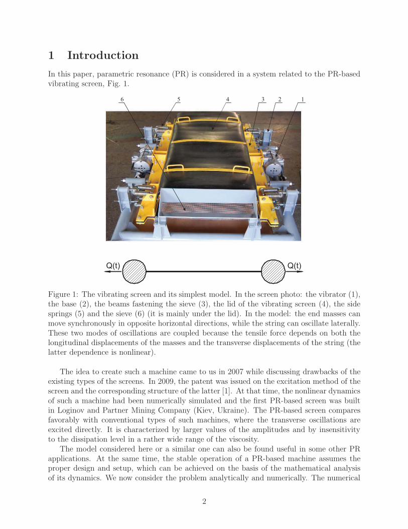
In this paper, parametric resonance (PR) is considered in a system related to the PR-basedvibrating screen, Fig. 1.

6 5 4 3 2 1

Q(t) Q(t)

Figure 1: The vibrating screen and its simplest model. In the screen photo: the vibrator (1),the base (2), the beams fastening the sieve (3), the lid of the vibrating screen (4), the sidesprings (5) and the sieve (6) (it is mainly under the lid). In the model: the end masses canmove synchronously in opposite horizontal directions, while the string can oscillate laterally.These two modes of oscillations are coupled because the tensile force depends on both thelongitudinal displacements of the masses and the transverse displacements of the string (thelatter dependence is nonlinear).

The idea to create such a machine came to us in 2007 while discussing drawbacks of theexisting types of the screens. In 2009, the patent was issued on the excitation method of thescreen and the corresponding structure of the latter [1]. At that time, the nonlinear dynamicsof such a machine had been numerically simulated and the first PR-based screen was builtin Loginov and Partner Mining Company (Kiev, Ukraine). The PR-based screen comparesfavorably with conventional types of such machines, where the transverse oscillations areexcited directly. It is characterized by larger values of the amplitudes and by insensitivityto the dissipation level in a rather wide range of the viscosity.

The model considered here or a similar one can also be found useful in some other PRapplications. At the same time, the stable operation of a PR-based machine assumes theproper design and setup, which can be achieved on the basis of the mathematical analysisof its dynamics. We now consider the problem analytically and numerically. The numerical

2

simulations serve for the refinement of the domains, where the parametric oscillations areexcited and where the analytically obtained steady oscillation regimes are stable. Both theanalytical and numerical simulations are used for the illustration and verification of theresults.

The problem is described by a system of two coupled nonlinear equations. We findan exact solution of these equations, which exists in the case of no damping associatedwith the transverse oscillations. This solution corresponds to an invariable tensile force.The equations appear uncoupled and linear; however, the solution is bounded and uniquelydefined by the fact that the nonlinearity in this established regime is zero. In a domain of theproblem parameters, it is stable due to the presence of the nonlinearity ‘in the background’.In this case, the coupling plays the role of a stabiliser. It is demonstrated numerically howthe transient regime approaches in time this established one defined analytically.

Next, we consider a more general, truly nonlinear regime. We use the harmonic analysiswith the higher harmonics neglected. In the considered case, the latter simplification has vir-tually no effect on the results obtained. Explicit expressions are found for the amplitudes oflongitudinal and transverse oscillations as functions of the external force amplitude and fre-quency. It is remarkable that in the case of the resonant excitation, where the external forcefrequency coincide with the frequency of the free longitudinal oscillations, the amplitudesare independent of the viscosity. In this regime, the nonlinearity bounds the amplitudes andthe damping provides the stability.

Along with the nonlinear problem, the boundaries of the PR domain in the frequency-amplitude plane are determined based on the linear formulation. The PR arises in thenonlinear problem practically in the frequency region predicted by the linear analysis, slightlyshifted towards the higher frequencies. It is shown that there is a sub region in this PRregion, where the analytically obtained steady oscillation regime is stable being reproducedin numerical simulations with a high accuracy. The steady PR regime can exist in a structuredependent range of the frequency with a moderate nonzero damping level. The transverseoscillations, regular or irregular, abruptly decaying on the boundaries do not exist outside ofthe PR region. Amplitude-frequency characteristics and some PR regimes realizations arepresented.

Before the forced PR regime we consider free oscillations of the perfect structure. Theperiodic energy exchange between the longitudinal and transverse modes of oscillations isdemonstrated. It is shown, in particular, that the period increases as the energy decreases.Note that this regime is, in a sense, similar to that for the spring pendulum system (Vittand Gorelik [2], Lai [3], Gaponov-Grekhov and Rabinovich [4]).

While in the past the parametric resonance has been mainly considered as an undesir-able phenomenon, some attempts were made to employ it to obtain a greater response toexcitation. Related problems were studied mainly (but not only) in the application to microdevices (see, e.g., Baskaran and Turner [5], Roads et al [6], Krylov [7], Krylov et al [8-10],Fey at al [11], Fossen and Nijmeijer [12], Plat and Busher [13] and the references therein).

3

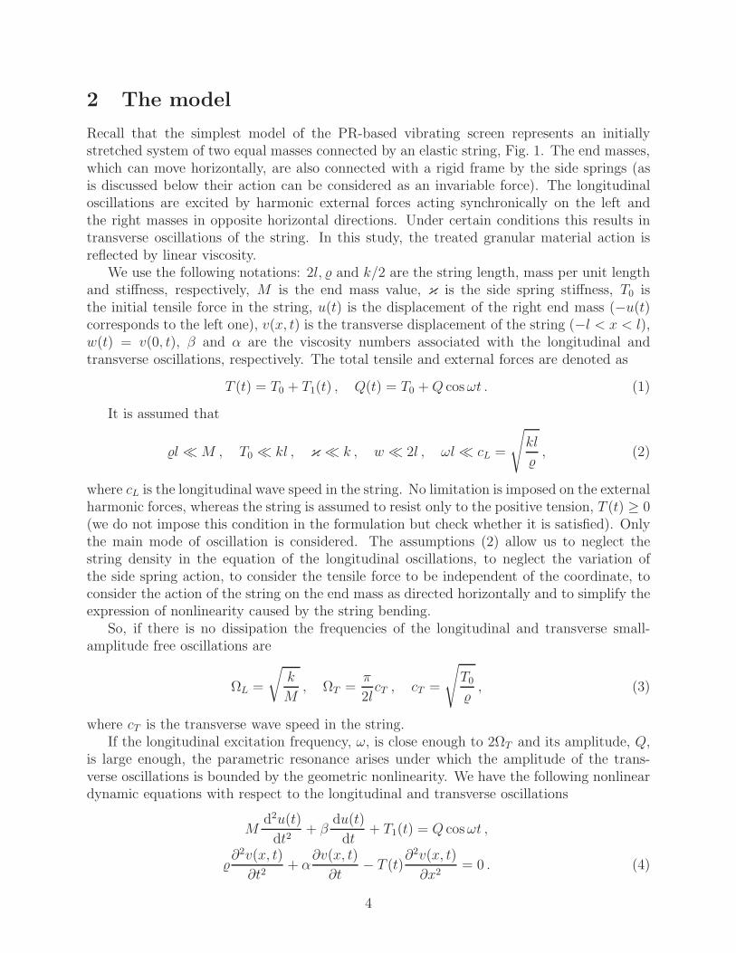
2 The model

Recall that the simplest model of the PR-based vibrating screen represents an initiallystretched system of two equal masses connected by an elastic string, Fig. 1. The end masses,which can move horizontally, are also connected with a rigid frame by the side springs (asis discussed below their action can be considered as an invariable force). The longitudinaloscillations are excited by harmonic external forces acting synchronically on the left andthe right masses in opposite horizontal directions. Under certain conditions this results intransverse oscillations of the string. In this study, the treated granular material action isreflected by linear viscosity.

We use the following notations: 2l, and k/2 are the string length, mass per unit lengthand stiffness, respectively, M is the end mass value, κ is the side spring stiffness, T0 isthe initial tensile force in the string, u(t) is the displacement of the right end mass (−u(t)corresponds to the left one), v(x, t) is the transverse displacement of the string (−l < x < l),w(t) = v(0, t), β and α are the viscosity numbers associated with the longitudinal andtransverse oscillations, respectively. The total tensile and external forces are denoted as

T (t) = T0 + T1(t) , Q(t) = T0 +Q cosωt . (1)

It is assumed that

l ≪M , T0 ≪ kl , κ ≪ k , w ≪ 2l , ωl ≪ cL =

√

kl

, (2)

where cL is the longitudinal wave speed in the string. No limitation is imposed on the externalharmonic forces, whereas the string is assumed to resist only to the positive tension, T (t) ≥ 0(we do not impose this condition in the formulation but check whether it is satisfied). Onlythe main mode of oscillation is considered. The assumptions (2) allow us to neglect thestring density in the equation of the longitudinal oscillations, to neglect the variation ofthe side spring action, to consider the tensile force to be independent of the coordinate, toconsider the action of the string on the end mass as directed horizontally and to simplify theexpression of nonlinearity caused by the string bending.

So, if there is no dissipation the frequencies of the longitudinal and transverse small-amplitude free oscillations are

ΩL =

√

k

M, ΩT =

π

2lcT , cT =

√

T0, (3)

where cT is the transverse wave speed in the string.If the longitudinal excitation frequency, ω, is close enough to 2ΩT and its amplitude, Q,

is large enough, the parametric resonance arises under which the amplitude of the trans-verse oscillations is bounded by the geometric nonlinearity. We have the following nonlineardynamic equations with respect to the longitudinal and transverse oscillations

Md2u(t)

dt2+ β

du(t)

dt+ T1(t) = Q cosωt ,

∂2v(x, t)

∂t2+ α

∂v(x, t)

∂t− T (t)

∂2v(x, t)

∂x2= 0 . (4)

4

These equations are coupled by the tensile force T1(t) which depends on both the longitudinaldisplacements of the masses, u(t) = u(t, l) = −u(t,−l), and the transverse displacement ofthe string, v(x, t)

T1(t) = k

[

u(t) +

∫ l

0

√

1 + (v′(x, t))2 dx− l

]

, (5)

where α and β are the viscosity numbers, v′(x, t) = ∂v(x, t)/∂x and expression (5) is validif it defines a nonnegative tensile force; otherwise, T (t) = 0. In this study, we consider theproblem assuming that this condition is satisfied; then we determine domains where this isso.

Clearly, the left side of the second equation in (4) with the boundary conditions, v(±l, t) =0, admits the variables separation as

v(x, t) = w(t) cosπx

2l. (6)

Using this expression and the condition concerning the amplitude of the transverse oscilla-tions in (2), the expression for the tensile force (5) can be reduces to

T1(t) = k

(

u(t) +π2

16lw2(t)

)

. (7)

The system of the dynamic equations becomes

Md2u(t)

dt2+ β

du(t)

dt+ T1(t) = Q cosωt ,

d2w(t)

dt2+ α

dw(t)

dt+π2

4l2T (t)w(t) = 0 . (8)

This system is the base of the below considerations. Note that this model and some itsgeneralizations were used in the numerical simulations while designing and setting of the PRvibrating screen. Being useful for the machine structure and setting pre-select it is also mostsuitable for the analytical study.

2.1 Energy relations

The sum of kinetic and potential energies of the system is

E =M [u(t)]2 +1

2l[w(t)]2 +

1

kT (t)2 − 2T0u(t) . (9)

With accuracy of a constant it is reduced to

E =M [u(t)]2 +1

2l[w(t)]2 +

1

kT1(t)

2 + T0π2

8lw2(t) . (10)

We consider the energy consisting of longitudinal and transverse parts as follows

E = Eu + Ew ,Eu =Mu2(t) +

1

kT 21 (t) (longitudinal part) ,

Ew =1

2lw2(t) +

π2

8lT0w

2(t) ( transverse part) . (11)

5

From this and the dynamic equations (8) we find the energy rates

Eu = 2(Mu(t) + T1)u(t) +π2

8lT1

dw2

dt= 2Qu(t) cosωt− 2β[u(t)]2 +

π2

8lT1

dw2(t)

dt,

Ew = lw(t)w(t) +π2

8lT0

dw2

dt= −αl[w(t)]2 − π2

8lT1

dw2(t)

dt. (12)

Recall that the nonlinear term is responsible for the energy exchange between the oscillationmodes.

2.2 Free oscillations

For free oscillations, Q = α = β = 0, we have

Eu = −Ew =π2

8lT1

dw2(t)

dt. (13)

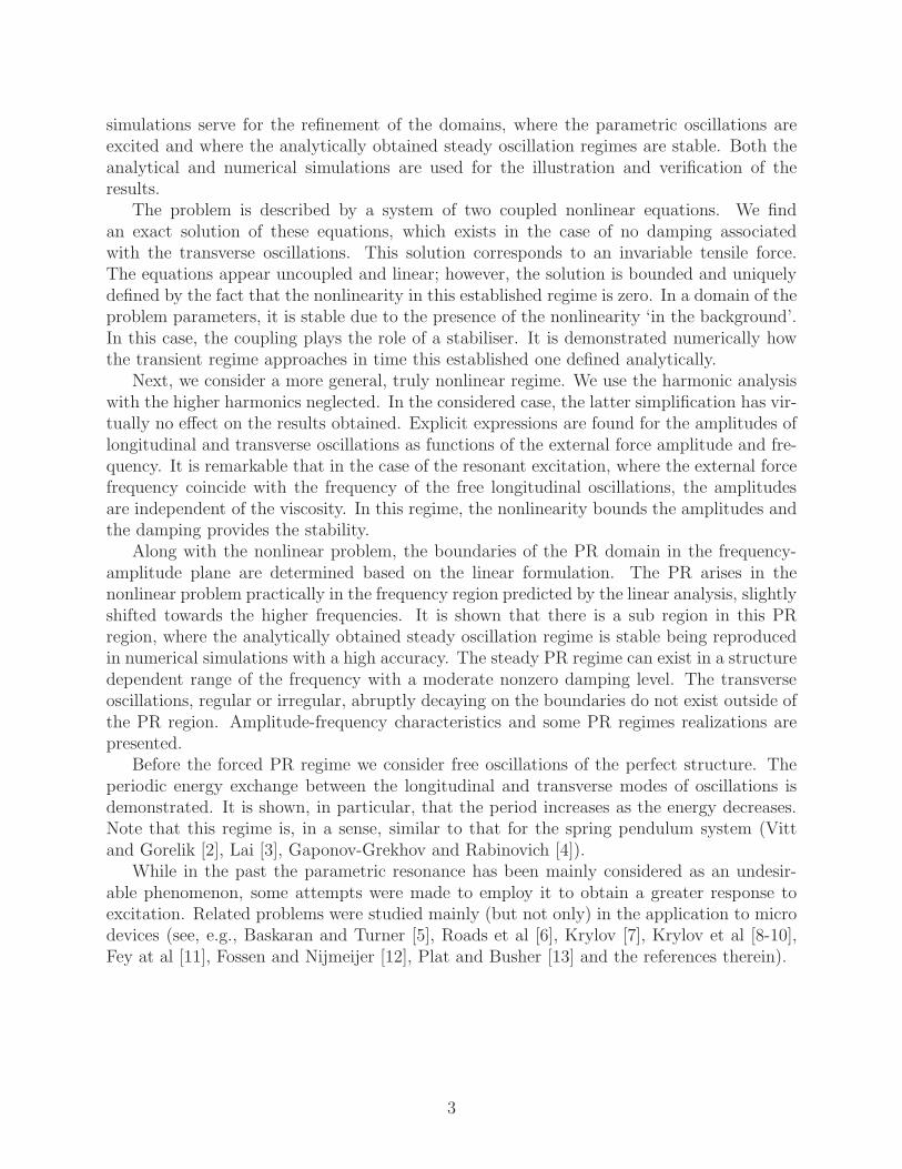
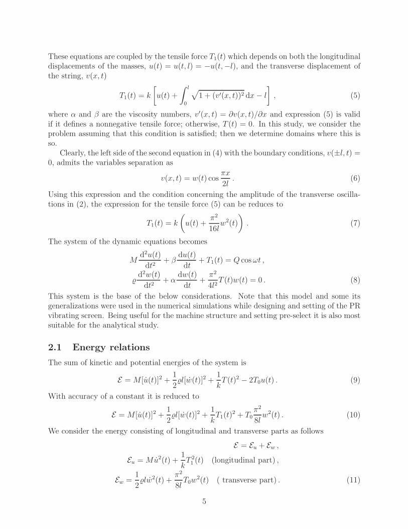
An example of the free oscillations and the energy exchange is shown in Fig. 2 and Fig. 3.The displacements, w(t)[m], u(t)[10−1m] and the energies, Eu,w[10−3Nm] are calculated forthe system with M=100 kg, =10 kg/m, T0=1 N, k=100 N/m, l=1 m (these units and asecond as the time-unit are used here and below), under the initial conditions w(0)=0.02 m,u(0) = w(0) = u(0) = 0.

w(t)u(t)

Figure 2: The transverse and longitudinal free oscillations, w(t)[m] and u(t)[10−1m].

Note that, in accordance with (13), the energy exchange period increases to infinity as theenergy decreases to zero. Indeed, for given dynamic parameters of the system the frequencyweakly depends on the energy, that is, on the oscillation amplitude; hence the derivative,dw2(t)/ dt is of the same order as w2 and the energy Ew, (11). The variable part of the tensileforce, T1, also decreases to zero as the energy. Thus, the derivative, Ew, decreases faster thanthe energy itself, that results in the increase of the energy exchange period. Numericalsimulations support the guess that the period is asymptotically inversely proportional to theenergy.

6

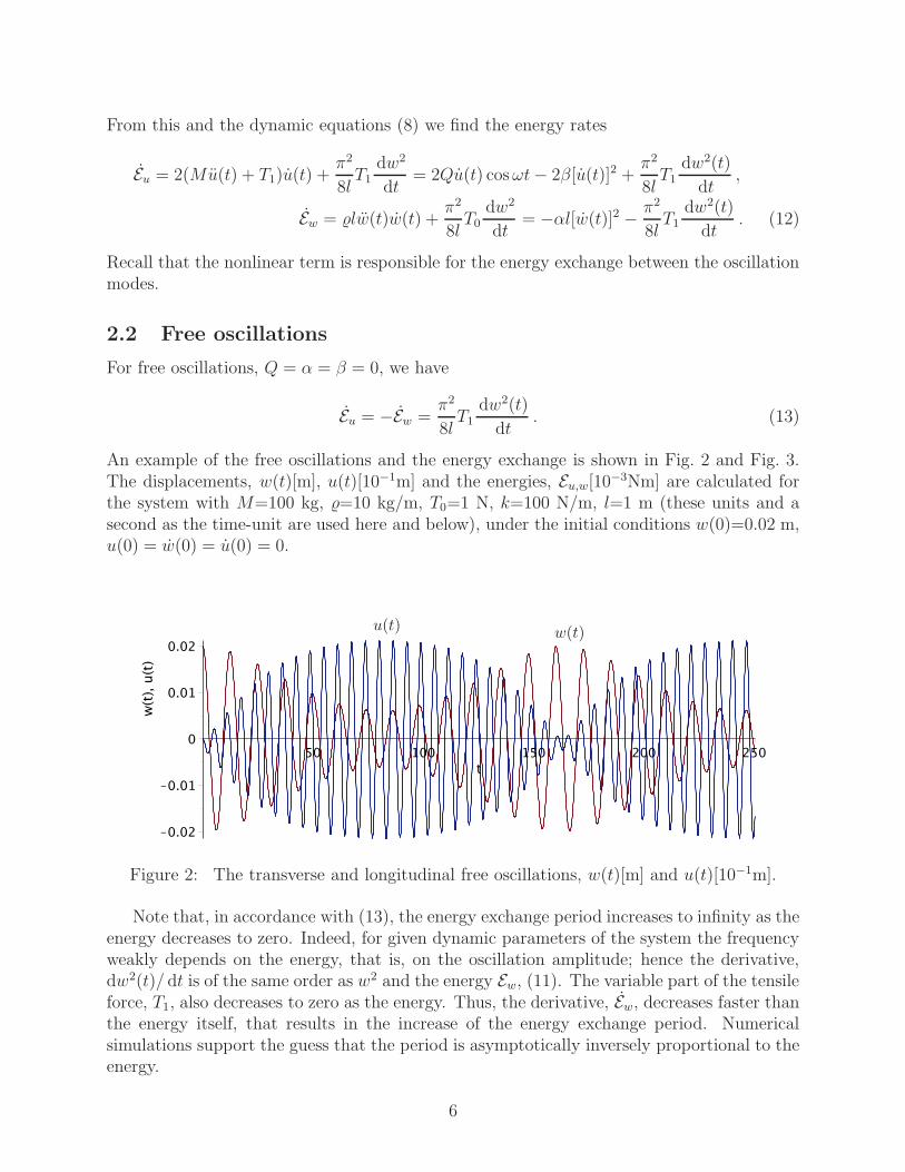
EwEu

Figure 3: . The energy exchange between the longitudinal and transverse free oscillations,Eu,w [10−3 Nm]. The ‘roughness’ of the curves is a consequence of numerous zeros of Eu,w.

3 An exact solution

It is interesting that there is an elementary exact solution of the system (8). It exists in thecase of the resonance excitation, ω = 2ΩT , of the model with no damping associated withthe lateral oscillations, α = 0. In this solution, the tensile force is invariable:

T (t) ≡ T0 , that is , T1 ≡ 0 . (14)

The corresponding equations are

Mu(t) + βu(t) = Q cosωt ,

w(t) +π2

4l2T0w(t) = 0 . (15)

We substitute the general solutions of these linear equations into the identity (14) and obtainthe oscillating displacements with a constant (negative) shift of u(t)

u(t) = − Q

ω(M2ω2 + β2)

(

Mω cosωt− β sinωt+√

M2ω2 + β2)

,

w(t) = A cosωt

2+B sin

ωt

2, T1(t) = 0 ,

A =

√

(

√

M2ω2 + β2 +Mω)

ψ , B =

√

(

√

M2ω2 + β2 −Mω)

ψ ,

ψ =16lQ

π2ω(M2ω2 + β2), (−u)max =

2Q

ω√

M2ω2 + β2,

wmax =4

π

√

2lQ

ω√

M2ω2 + β2=

4

π

√

l(−u)max , ω = 2ωT . (16)

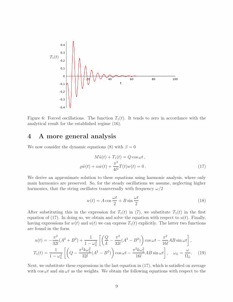
At least in a certain domain of the initial conditions, the transient solutions based on theequations (8) with α = 0 approach in time the above presented one based on the equations(14), (15). This is justified by numerical simulations of the transient problem with initialconditions inconsistent with the identity (14). The numerically obtained oscillations and theoscillation amplitude found analytically from (14), (15) are presented in Fig. 4, Fig. 5 and

7

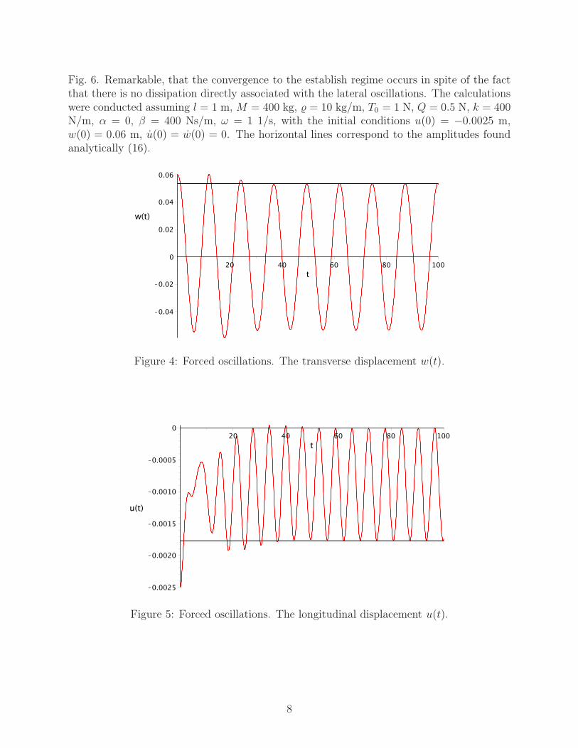
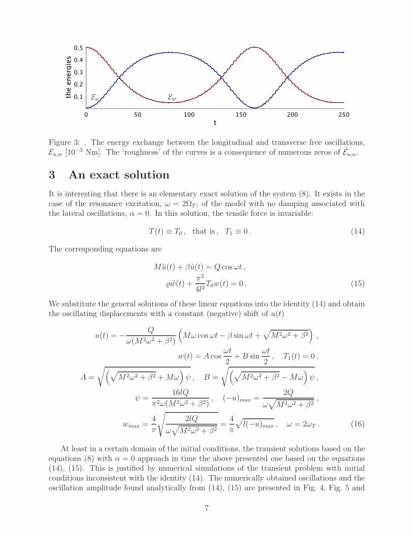
Fig. 6. Remarkable, that the convergence to the establish regime occurs in spite of the factthat there is no dissipation directly associated with the lateral oscillations. The calculationswere conducted assuming l = 1 m, M = 400 kg, = 10 kg/m, T0 = 1 N, Q = 0.5 N, k = 400N/m, α = 0, β = 400 Ns/m, ω = 1 1/s, with the initial conditions u(0) = −0.0025 m,w(0) = 0.06 m, u(0) = w(0) = 0. The horizontal lines correspond to the amplitudes foundanalytically (16).

Figure 4: Forced oscillations. The transverse displacement w(t).

Figure 5: Forced oscillations. The longitudinal displacement u(t).

8

T1(t)

Figure 6: Forced oscillations. The function T1(t). It tends to zero in accordance with theanalytical result for the established regime (16).

4 A more general analysis

We now consider the dynamic equations (8) with β = 0

Mu(t) + T1(t) = Q cosωt ,

w(t) + αw(t) +π2

4l2T (t)w(t) = 0 . (17)

We derive an approximate solution to these equations using harmonic analysis, where onlymain harmonics are preserved. So, for the steady oscillations we assume, neglecting higherharmonics, that the string oscillates transversally with frequency ω/2

w(t) = A cosωt

2+B sin

ωt

2(18)

After substituting this in the expression for T1(t) in (7), we substitute T1(t) in the firstequation of (17). In doing so, we obtain and solve the equation with respect to u(t). Finally,having expressions for w(t) and u(t) we can express T1(t) explicitly. The latter two functionsare found in the form

u(t) = − π2

32l(A2 +B2) +

1

1− ω2L

[(

Q

k− π2

32l(A2 − B2)

)

cosωt− π2

16lAB sinωt

]

,

T1(t) =1

1− ω2L

[(

Q− π2kω2L

32l(A2 − B2)

)

cosωt− π2kω2L

16lAB sinωt

]

, ωL =ω

ΩL

. (19)

Next, we substitute these expressions in the last equation in (17), which is satisfied on averagewith cosωt and sinωt as the weights. We obtain the following equations with respect to the

9

coefficients

π2

4l2A

[

1

1− ω2L

(

Q

2T0− π2kω2

L

64lT0(A2 +B2)

)

+

(

1− ω2T

4

)]

+αω

2T0B = 0 ,

π2

4l2B

[

1

1− ω2L

(

Q

2T0+π2kω2

L

64lT0(A2 +B2)

)

−(

1− ω2T

4

)]

+αω

2T0A = 0 ,

ωL = ω/ΩL , ωT = ω/ΩT . (20)

From this the following solution is found

B = γA , γ = −κ

(

1−√

1− 1

κ2

)

, κ =π2Q

4αωl2(1− ω2L)

(21)

and

A = ± 8l

πωL

√

1 + γ2

√

Q

2kl

√

1− 1

κ2+T0kl

(

1− ω2T

4

)

(1− ω2L) . (22)

It can be seen, in particular, that under the resonant excitation, ωL = 1, the amplitude isindependent of both the transverse oscillation frequency, ΩT , and the viscosity level. Indeed,κ → ∞ , γ → 0 (ωL → 1), and in the limit

A = ±4l

π

√

2Q

kl, B = 0 (ωL = 1) . (23)

The solution (21) - (23) is valid in a domain, where the considered stationary oscillationregime really exists, that is, where it is stable. Below this issue is discussed in more detail.

Functions u(t) and T1(t) for ωL 6= 1 are defined in (19). The limits at ωL = 1 are

u(t) = −Qk+

[

2T0k

(

1− ω2T

4

)

− Q

k

]

cosωt+4αωl2

π2ksinωt ,

T1(t) = −2T0

(

1− ω2T

4

)

cosωt+4αωl2

π2sinωt . (24)

If, in addition, α = 0 and ωT = 2 (ΩT = ΩL/2) then T1 = 0, and we come back to theabove-considered exact solution (16) (with β = 0).

4.1 Energy flux

In the above-considered general case with β = 0, the energy dissipation rate averaged overthe period of oscillations is

D = 2α

∫ l

0

〈v(x, t)2〉 dx =αω2l

8(A2 +B2) =

αω2l(1 + γ2)

8A2 = −αω

2lκγ

4A2 . (25)

On the other hand, it follows from (19) that the energy flux produced by the external forceis

N = 2Q〈u(t) cosωt〉 = − π2ωγ

16l(1− ω2L)A2Q . (26)

Referring to (21) we see that these quantities coincide as it should be.

10

5 Parametric resonance domains

Neglecting nonlinear terms in equations (20) we obtain an approximate expression for themain resonance domain boundary on the (ω,QL) plane

Q = QL = ±2T0(1− ω2L)

√

(

2αωl2

π2T0

)2

+

(

1− ω2T

4

)2

. (27)

Note that here κ2 ≥ 1. In addition to this bound, the nonlinear analytical solution itself is

bounded by the condition T (t) ≥ 0, which is not satisfied if κ2 < 1.

5.1 Dimensionless formulation

We now introduce the dimensionless amplitude of w(t), A, and the other quantities

A =Al=A√

1 + γ2

l, (u, w) =

(u, w)

l, t = t

√

k

M, ω = ω

√

M

k,

α =α

√

M

k, β =

β√kM

, (T (t), Q) =(T (t), Q)

kl, λ =

kl

T0, µ =

l

M. (28)

In these terms,

ΩL = 1 , ωL = ω , ΩT =π

2√λµ

, κ =π2Q

4µ(1− ω2)αω. (29)

The dynamic equations (8) take the form (in the below relations, the hat symbol is omitted)

u(t) + βu(t) + u(t) +π2

16w2(t) = Q cosωt ,

w(t) + αw(t) + Ω2T

[

1 + λ

(

u(t) +π2

16w2(t)

)]

w(t) = 0 (30)

and

A = ± 8

πω√

1 + γ2

√

Q

2

√

1− 1

κ2+

1

λ

(

1− ω2T

4

)

(1− ω2) . (31)

The ω −QL relation (27) becomes

QL = ±2

λ|1− ω2|

√

(

1− ω2T

4

)2

+

(

2

π2λµαω

)2

. (32)

Some plots corresponding to this expression are presented in Fig. 7.

11

ω

QL

1 2 3 4 5 6

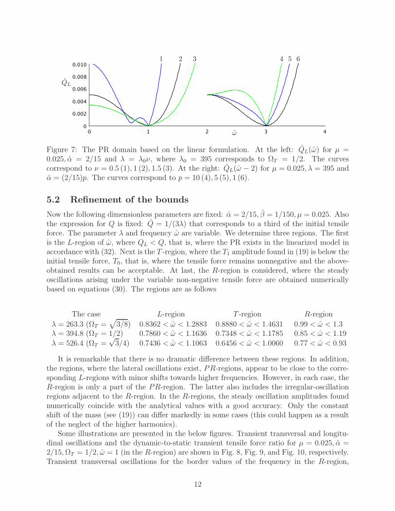
Figure 7: The PR domain based on the linear formulation. At the left: QL(ω) for µ =0.025, α = 2/15 and λ = λ0ν, where λ0 = 395 corresponds to ΩT = 1/2. The curvescorrespond to ν = 0.5 (1), 1 (2), 1.5 (3). At the right: QL(ω − 2) for µ = 0.025, λ = 395 andα = (2/15)p. The curves correspond to p = 10 (4), 5 (5), 1 (6).

5.2 Refinement of the bounds

Now the following dimensionless parameters are fixed: α = 2/15, β = 1/150, µ = 0.025. Alsothe expression for Q is fixed: Q = 1/(3λ) that corresponds to a third of the initial tensileforce. The parameter λ and frequency ω are variable. We determine three regions. The firstis the L-region of ω, where QL < Q, that is, where the PR exists in the linearized model inaccordance with (32). Next is the T -region, where the T1 amplitude found in (19) is below theinitial tensile force, T0, that is, where the tensile force remains nonnegative and the above-obtained results can be acceptable. At last, the R-region is considered, where the steadyoscillations arising under the variable non-negative tensile force are obtained numericallybased on equations (30). The regions are as follows

The case L-region T -region R-region

λ = 263.3 (ΩT =√

3/8) 0.8362 < ω < 1.2883 0.8880 < ω < 1.4631 0.99 < ω < 1.3λ = 394.8 (ΩT = 1/2) 0.7860 < ω < 1.1636 0.7348 < ω < 1.1785 0.85 < ω < 1.19

λ = 526.4 (ΩT =√3/4) 0.7436 < ω < 1.1063 0.6456 < ω < 1.0060 0.77 < ω < 0.93

It is remarkable that there is no dramatic difference between these regions. In addition,the regions, where the lateral oscillations exist, PR-regions, appear to be close to the corre-sponding L-regions with minor shifts towards higher frequencies. However, in each case, theR-region is only a part of the PR-region. The latter also includes the irregular-oscillationregions adjacent to the R-region. In the R-regions, the steady oscillation amplitudes foundnumerically coincide with the analytical values with a good accuracy. Only the constantshift of the mass (see (19)) can differ markedly in some cases (this could happen as a resultof the neglect of the higher harmonics).

Some illustrations are presented in the below figures. Transient transversal and longitu-dinal oscillations and the dynamic-to-static transient tensile force ratio for µ = 0.025, α =2/15,ΩT = 1/2, ω = 1 (in the R-region) are shown in Fig. 8, Fig. 9, and Fig. 10, respectively.Transient transversal oscillations for the border values of the frequency in the R-region,

12

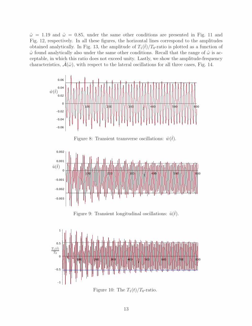
ω = 1.19 and ω = 0.85, under the same other conditions are presented in Fig. 11 andFig. 12, respectively. In all these figures, the horizontal lines correspond to the amplitudesobtained analytically. In Fig. 13, the amplitude of T1(t)/T0-ratio is plotted as a function ofω found analytically also under the same other conditions. Recall that the range of ω is ac-ceptable, in which this ratio does not exceed unity. Lastly, we show the amplitude-frequencycharacteristics, A(ω), with respect to the lateral oscillations for all three cases, Fig. 14.

w(t)

t

Figure 8: Transient transverse oscillations: w(t).

u(t)

t

Figure 9: Transient longitudinal oscillations: u(t).

T1(t)T0

t

Figure 10: The T1(t)/T0-ratio.

13

w(t)

t

Figure 11: Transient transverse oscillations on the upper bound of R-region: w(t) forµ = 0.025, α = 2/15,ΩT = 1/2, ω = 1.19. In this case, the oscillation amplitudes quicklyapproach the values found analytically.

w(t)

t

Figure 12: Transient transverse oscillations on the lower bound of R-region: w(t) for µ =0.025, α = 2/15,ΩT = 1/2, ω = 0.85. In this case, the oscillation amplitudes slowly approachthe values found analytically.

Tmax

T0

ω

Figure 13: The amplitude of T1(t)/T0-ratio as a function of ω found analytically for µ =0.025, α = 2/15,ΩT = 1/2. Recall that the range of ω is acceptable, where it is less thanunity.

14

1 2 3A

φ

Figure 14: The analytically obtained amplitude of w(t): A(ω) for µ = 0.025, α = 2/15. Thecurves correspond to ΩT =

√3/4, ω = φ (1); ΩT = 1/2, ω = φ − 0.08 (2) and ΩT =

√

3/8,ω = φ− 0.28 (3).

The right limiting point in Fig. 14, where A = 0 (ω ≈ 1.31), limits the region whereregular PR oscillations can be excited (κ2 < 1 for greater ω, and the solution (22) failed).

6 Conclusion

The solutions obtained in this paper allow seeing how the system parameters affect thevibration level. For example, let the excitation frequency be resonant with respect to thelateral oscillations, ωT = 2, and κ

2 > 1. It can be seen from (22) (also see (3), (19) and(21)) that the amplitude, A, increases unboundedly as the end mass, M , decreases. Indeed,ΩL ∼ 1/

√M and A ∼ 1/ωL ∼ 1/

√M . Note, however, that “proportional” (∼) remains

asymptotically valid only for small amplitudes. In addition, the results allow to estimatethe PR domains with steady oscillations and to determine the corresponding amplitude-frequency characteristics as was demonstrated in the paper.

In designing and setting a PR-based machine, a simple model used in this paper maybe not sufficient, mainly because the interaction with the treated granular material is notincluded in the dynamic equations explicitly (only damping reflects this interaction). Aproperly developed model appears difficult for the analytical study. In this case, numeri-cal simulations can be effective (as in designing of PR-based vibrating screen in LPMC),whereas the above-obtained results based on a simple model may be useful for preliminaryestimations.

Acknowledgement. This paper has been written while V.I. Slepyan held a short-termvisiting research position at Tel Aviv University in the framework of the project “VIBRO-IMPACT MACHINES BASED ON PARAMETRIC RESONANCE: Concepts, mathemati-cal modelling, experimental verification and implementation”, 01/01/2012-31/12/2015. Wethankful for the support provided by FP7-People-2011-IAPP, Marie Curie Actions, GrantNo. 284544,http://www.openaire.eu/fr/component/openaire/project info/default/530?grant=284544 .

15

References

[1] V.I. Slepyan, I.G. Loginov and L.I. Slepyan, The method of resonance excitation ofa vibrating sieve and the vibrating screen for its implementation. Ukrainian patent oninvention No. 87369, 2009.[2] A.A. Vitt and G.S. Gorelik, Oscillations of an elastic pendulum as an example of theoscillations of two parametrically coupled linear systems. Journal of Technical Physics, 3(1933) 294–307 (originally published in the Russian journal Zhurnal Tekhnicheskoy Fiziki, 3(1933) 294–307).[3] H.M. Lai, On the recurrence phenomenon of a resonant spring pendulum. Am. J. Phys.52 (1984) 219-223.[4] A.V. Gaponov-Grekhov, M.I. Rabinovich, Nonlinearities in action. Springer-Verlag,Berlin, London, 1992.[5] R. Baskaran and K. L. Turner, Mechanical domain coupled mode parametric resonanceand amplification in a torsional mode micro electro mechanical oscillator. J. Micromech.Microeng. 13 (2003) 701707.[6] J.F. Rhoads, S.W. Shaw, K.L. Turner, R. Baskaran, Tunable microelectromechanicalfilters that exploit parametric resonance. Journal of Vibration and Acoustics 127 (2005)423-430.[7] S. Krylov, Parametric excitation and stabilization of electrostatically actuated microstruc-tures. Int. J. Microscale Computational Engineering 6 (2008) 563-584.[8] S. Krylov, I. Harari, and Y. Cohen, Stabilization of electrostatically actuated microstruc-tures using parametric excitation. J. Micromech. Microeng 15 (2005) 11881204.[9] S. Krylov, Y.Gerson, T. Nachmias,, and U. Keren, Excitation of large-amplitude para-metric resonance by the mechanical stiffness modulation of a microstructure. J. Micromech.Microeng 20 (2010) 1-12, 015041 doi:10.1088/0960-1317/20/1/015041.[10] S. Krylov, N. Molinazzib, T. Shmilovicha, U. Pomerantza, S. Lulinskya, Parametricexcitation of flexible vibrations of micro beams by fringing electrostatic fields. Proceedingsof the ASME 2010 International Design Engineering Technical Conferences & Computersand Information in Engineering Conference IDETC/CIE 2010. Montreal, Quebec, Canada,601-611, 2010.[11] Fey, R.H.B., Mallon, N.J., Kraaij, C.S., and Nijmeijer, H., Nonlinear resonances inan axially excited beam carrying a top mass : simulations and experiments. NonlinearDynamics, 66(3) (2011), 285-302.[12] Fossen, T.I., and Nijmeijer, H., Parametric resonance in dynamical systems, Springer,New York, 2012.[13] H.Plat, I. Bucher, Optimizing parametric oscillators with tunable boundary conditions.J. of Sound and Vibration, 332 (2013) 487493.

16