A deterministic map of Waddington's epigenetic landscape for cell fate specification

A deterministic map of Waddington's epigeneticlandscape for cell fate specificationBhattacharya et al.

Bhattacharya et al. BMC Systems Biology 2011, 5:85http://www.biomedcentral.com/1752-0509/5/85 (27 May 2011)

RESEARCH ARTICLE Open Access

A deterministic map of Waddington’s epigeneticlandscape for cell fate specificationSudin Bhattacharya*, Qiang Zhang and Melvin E Andersen

Abstract

Background: The image of the “epigenetic landscape”, with a series of branching valleys and ridges depictingstable cellular states and the barriers between those states, has been a popular visual metaphor for cell lineagespecification - especially in light of the recent discovery that terminally differentiated adult cells can bereprogrammed into pluripotent stem cells or into alternative cell lineages. However the question of whether theepigenetic landscape can be mapped out quantitatively to provide a predictive model of cellular differentiationremains largely unanswered.

Results: Here we derive a simple deterministic path-integral quasi-potential, based on the kinetic parameters of agene network regulating cell fate, and show that this quantity is minimized along a temporal trajectory in the statespace of the gene network, thus providing a marker of directionality for cell differentiation processes. We then usethe derived quasi-potential as a measure of “elevation” to quantitatively map the epigenetic landscape, on whichtrajectories flow “downhill” from any location. Stochastic simulations confirm that the elevation of this computedlandscape correlates to the likelihood of occurrence of particular cell fates, with well-populated low-lying “valleys”representing stable cellular states and higher “ridges” acting as barriers to transitions between the stable states.

Conclusions: This quantitative map of the epigenetic landscape underlying cell fate choice provides mechanisticinsights into the “forces” that direct cellular differentiation in the context of physiological development, as well asduring artificially induced cell lineage reprogramming. Our generalized approach to mapping the landscape isapplicable to non-gradient gene regulatory systems for which an analytical potential function cannot be derived,and also to high-dimensional gene networks. Rigorous quantification of the gene regulatory circuits that governcell lineage choice and subsequent mapping of the epigenetic landscape can potentially help identify optimalroutes of cell fate reprogramming.

BackgroundThe biologist Conrad Hal Waddington, in the course ofa career spanning four decades (1930s - 1970s),attempted a bold synthesis of the fields of genetics,embryology and evolution [1,2]. The centerpiece of hisvision was the idea of the “epigenetic landscape”, firstdescribed in An Introduction to Modern Genetics [3],and elaborated in subsequent monographs [4,5]. Wad-dington portrayed the epigenetic landscape as aninclined surface with a cascade of branching ridges andvalleys (Figure 1A), which in the context of cell lineageselection, represent the series of “either/or” fate choicesmade by a developing cell. He envisioned that on this

landscape, “the presence or absence of particular genesacts by determining which path shall be followed from acertain point of divergence [1,4]“, thus providing in asingle image an appealing, and influential, metaphor forthe connection between genotype and phenotype.In the quantitative view of a cell as a dynamical sys-

tem governed by genetic interaction networks [6], anintuitive association can be made between the valleys("creodes” in Waddington’s terminology) on the epige-netic landscape and the trajectories leading to theattractors, or stable steady states, of the gene networksthat regulate cell fate [7-9]. But can we quantitativelymap the undulating surface of the landscape, therebyproviding a predictive model of the “directionality” ofcellular differentiation? Waddington himself cautionedthat the epigenetic landscape, while useful as a “rough

* Correspondence: [email protected] of Computational Biology, Program in Chemical Safety Sciences, TheHamner Institutes for Health Sciences, Research Triangle Park, NC 27709, USA

Bhattacharya et al. BMC Systems Biology 2011, 5:85http://www.biomedcentral.com/1752-0509/5/85

© 2011 Bhattacharya et al; licensee BioMed Central Ltd. This is an Open Access article distributed under the terms of the CreativeCommons Attribution License (http://creativecommons.org/licenses/by/2.0), which permits unrestricted use, distribution, andreproduction in any medium, provided the original work is properly cited.

mailto:[email protected]

http://creativecommons.org/licenses/by/2.0

and ready picture” of development, “cannot be inter-preted rigorously [5]“. The mathematician René Thom,in his formulation of catastrophe theory inspired byWaddington’s ideas, proposed that a generalized “poten-tial surface” could be derived for any dynamical system[2,10]. However Thom’s later writings suggest that hedid not believe it possible to quantify the epigeneticlandscape [11]. This view has been echoed by otherauthors, who have described the landscape as a “colorfulmetaphor [2]“ with “no grounding in physical reality[1]“.Huang, Wang and colleagues have recently proposed a

probabilistic “pseudo-potential” to quantify the epige-netic landscape for a gene network regulating cell fate,where the elevation of the surface is inversely related tothe likelihood of occurrence of a particular state inphase space [8,12,13]. In this formulation a stochasticpotential energy landscape is characterized for a genenetwork, based on a Hartree mean-field approximationof the underlying master equation [14]. Such stochasticformulations have also been used to derive probabilisticpotential landscapes for the lysis-lysogeny switch in bac-teriophage lambda [15-17], the mitogen-activated pro-tein kinase (MAPK) signal transduction network [18],biochemical oscillations [19], and the predator-prey sys-tem [20].Here we propose a simple numerical method to map

the epigenetic landscape that is not based on a probabil-istic or master-equation approach. Instead, a quasi-potential surface (Figure 1B) is derived directly from thedeterministic rate equations governing the dynamicbehavior of a gene regulatory circuit. We then use sto-chastic simulations to show that the elevation of thiscomputed landscape correlates to the likelihood ofoccurrence of particular cell fates, with well-populatedlow-lying valleys representing stable cellular states and

higher ridges acting as barriers to transitions betweenthe stable states.Finally, we discuss ways in which this quantitatively

mapped landscape may help predict the efficiency of cel-lular de-differentiation or trans-differentiation, and iden-tify optimal routes of cell fate reprogramming. Recentdiscoveries have challenged the dogma of cell fate deter-mination as a unidirectional and irreversible process.Even terminally differentiated adult cells have now beenshown to retain considerable phenotypic plasticity andthe ability to be reprogrammed into pluripotent stemcell-like states [21-27] or into alternative differentiatedlineages [28-34] by forced expression of a single gene ora small number of genes. These findings have led to aresurgence of interest in Waddington’s ideas about celllineage choice, with several authors invoking the imageof the epigenetic landscape [7-9,35-39]. However thetheoretical basis of plasticity in cell fate is still not fullyunderstood, and the efficiency of reprogramming inthese studies is often quite low [36]. A quantitativeunderstanding of the “forces” that drive cell differentia-tion, and the “barriers” that separate stable cell states, isurgently needed. Such understanding may eventuallyenable us to predict the relative ease or difficulty of de-differentiation or trans-differentiation among multiplecellular states.

Results and DiscussionDerivation of the quasi-potential landscapeWe first illustrate our quantitative approach with a sim-ple circuit of two genes x and y that inhibit each other,forming a double-negative feedback loop structure (seeMethods). This circuit works as a toggle switch withtwo stable steady states: one state with high y and low xexpression, and the other state with high x and low yexpression [40]. Such “bistable” switches formed by

Figure 1 Mapping Waddington’s epigenetic landscape. (A) The “epigenetic landscape” proposed by Conrad Waddington shows a ball rollingdown valleys separated by ridges on an inclined surface, as a visual metaphor for the branching pathways of cell fate determination. Figurereproduced from original text by Waddington [5]. (B) The computed epigenetic landscape for a two-gene (x and y) regulatory network withmutual inhibition and positive autoregulation, where the elevation represents a path-integral quasi-potential derived from the deterministic rateequations describing the interactions of the two genes. We show that the “valleys” on this computed surface correspond to stable steady states(attractors) of the network, while the “ridges” separating the valleys represent barriers to stochastic transitions among multiple steady states.Colored circles represent a population of stochastically simulated “cells” (multiple instances of the network) residing in different stable steadystates.


Page 2 of 11

mutual antagonism of a pair of key regulatory genesunderlie many binary cell fate choices [7,13]. The circuitcan be described as a two-variable dynamical system,with the rate of change in expression of each of the twogenes given as a function of their expression levels:

dxdt

= f (x, y)

dydt

= g(x, y)(1)

If we were able to derive a closed-form potential func-tion V(x,y) for the system in Eq. 1 that satisfied the con-ditions:

∂V∂x

= −dxdt

∂V∂y

= −dydt

(2)

then the local minima on the two-variable potentialsurface V(x,y) would correspond mathematically to thestable steady states of the system, given that at the localminima on the surface (∂V/∂x = 0; ∂V/∂y = 0), the ratesof change in expression of both genes x and y would bezero (per Eq. 2). But such a closed-form potential func-tion can be derived only in the case of a gradient system,defined by the condition [41]:

∂f (x, y)∂y

=∂g(x, y)

∂x(3)

In general, condition (3) will not be valid for an arbi-trary circuit of two genes x and y that regulate eachother as per Eq. 1, making it impossible to derive aclosed-form potential function.Therefore, given that a gene circuit is in general a

non-gradient system, we define a term Vq that changesincrementally along a trajectory followed by the systemin x-y phase space (Figure 2A) as follows:

�Vq =∂Vq

∂x· �x +

∂Vq

∂y· �y

= −dxdt

· �x − dydt

· �y

(4)

where Δx and Δy are sufficiently small increments

along the trajectory such thatdxdt

anddydt

can be assumed

to remain unchanged over the interval [(x, x+Δx); (y, y+Δy)]. The quantities Δx and Δy are obtained as the

productsdxdt

· �t anddydt

· �t, respectively, where Δt is

the time increment. We use the term “quasi-potential”to describe Vq, to emphasize its distinction from aclosed-form potential function.

The change in the quasi-potential, Δ Vq, can berewritten from Eq. 4 as:

�Vq = −dxdt

·(

dxdt

· �t)

− dydt

·(

dydt

· �t)

= −[(

dxdt

)2

+(

dydt

)2]

· �t(5)

For positive increments in time Δt, Δ Vq is thusalways negative along an evolving trajectory, ensuringthat trajectories flow “downhill” along a putative “quasi-potential surface”. Stable steady states of the system (dx/dt = 0; dy/dt = 0) would correspond to local minima onthis quasi-potential surface, given that at these states ΔVq = 0 (per Eq. 5). The overall change in the quasi-potential along a trajectory can then be calculated bynumerically integrating the quantity Δ Vq in Eq. 4 froma given initial configuration up to a stable steady state,thereby allowing us to map out a temporal trajectoryalong the putative quasi-potential surface (Figure 2B).The quasi-potential thus defined is a measurable quan-tity that is minimized along a trajectory from any initialcondition to an attractor in the phase space of the twogenes, and is in effect a Liapunov function of the dyna-mical system represented by the two-gene circuit [41].The procedure described above was repeated to evalu-

ate the change in the quasi-potential along trajectoriesoriginating from different points in x-y phase space. Toderive a quasi-potential surface from multiple trajec-tories, we then make the following assumptions: (i) twotrajectories with different initial conditions that con-verge to the same steady state must also converge to thesame final quasi-potential level (Figure 2B); (ii) two tra-jectories that originate from “adjacent” initial conditionsthat are sufficiently close in x-y phase space, but con-verge to different steady states, must start from thesame initial quasi-potential level (Figure 2C). Observa-tion (i) allows us to map out a basin of attraction frommultiple trajectories converging to a single steady state;while observation (ii) enables the alignment of two adja-cent basins of attraction along their shared basin bound-ary, or separatrix. (Essentially, (i) and (ii) togetheramount to the assumption that the putative epigeneticlandscape is continuous.) The quasi-potential surfacecan then be obtained by interpolation among the alignedtrajectories (Figure 2D, E), yielding the epigeneticlandscape with its characteristic ridges and valleys(Figure 3A, B).The same procedure can be applied to systems with

more than two stable steady states - for instance, a “tris-table” system produced by a circuit of two genes thatinduce their own expression, in addition to mutual inhi-bition (Figure 3C, D). This system has three steady


Page 3 of 11

Figure 2 Computing the epigenetic landscape for a bistable switch based on a double-negative feedback circuit of two genes x and y.(A) Paths followed by a simulated cell on the epigenetic landscape are obtained by integrating the change in quasi-potential ΔVq (Eq. 4 in text)along a trajectory as a function of time. (x+Δx) and (y+Δy) give the new position at each step along the trajectory in x-y phase space, while (Vq+ΔVq) gives the new elevation on the quasi-potential surface. The initial value of the quasi-potential at the start of any individual trajectory isarbitrarily set to zero. (B) Two trajectories (1 and 2) that converge to the same attractor on the x-y phase plane are aligned vertically so thatboth trajectories also converge to the same quasi-potential level. (C) Two trajectories that originate at adjacent points on the phase plane butconverge to different attractors A and B are aligned vertically so that the initial quasi-potential levels of the two trajectories are equal. (D)Multiple trajectories starting from different points on the x-y phase plane are then aligned as described in panels B and C. To identify distinctbasins of attraction, trajectories are shown colored according to the attractor to which they converge (arrows). This two-gene double-negativefeedback circuit produces a bistable system with two attractors A and B. (E) Finally, interpolation among multiple trajectories aligned across thephase plane produces the epigenetic landscape.


Page 4 of 11

states - two of which represent alternative differentiatedcell lineages, while the third state depicts the commonprogenitor cell of the two lineages [8,13,42].

Quantitative interpretation of the quasi-potentiallandscapeTo establish that the “elevation” of the computed land-scape at a given location in x-y phase space correlatesinversely to the probability of occurrence of the corre-sponding network state, we used stochastic simulations[43] of the underlying gene network. These simulations,which take into account fluctuations in gene expressionlevels [44] in a population of simulated “cells” (multipleinstances of the gene network), showed that the “valleys”

of low elevation on the computed epigenetic landscapecorrespond to stable cellular states, with “deeper” valleysassociated with higher probability of occupancy thanshallower valleys (Figure 4A-D). On the other hand, the“ridges” separating the valleys represent barriers to sto-chastic transitions between multiple steady states. Vary-ing the parameters in the network model to increase theheight of the ridges relative to the valleys dramaticallyreduced the probability of transitions between the steadystates (Figure 5), even though there was no appreciablechange in the relative distance between the steady stateson the x-y phase plane (Figure 4A-D, right panels).The “third dimension” (elevation) of the landscape

represented by the quasi-potential, although directly

Figure 3 Ridges and valleys on the computed epigenetic landscape of a bistable (A, B) and a tristable (C, D) regulatory network oftwo genes x and y. The alignment of trajectories produces the “ridges” on the epigenetic landscape (indicated by arrows in panels B and D)that separate the “valleys”, or basins of attraction of multiple stable states of the network (points A, B and C). Equi-potential lines are drawn onthe landscape to depict the curvature of the surface. In addition to the double-negative feedback loop between genes x and y that producesthe bistable network (panels A and B), the tristable network (panels C and D) requires additional positive autoregulation of the two genes[8,13,42] (see Methods).


Page 5 of 11

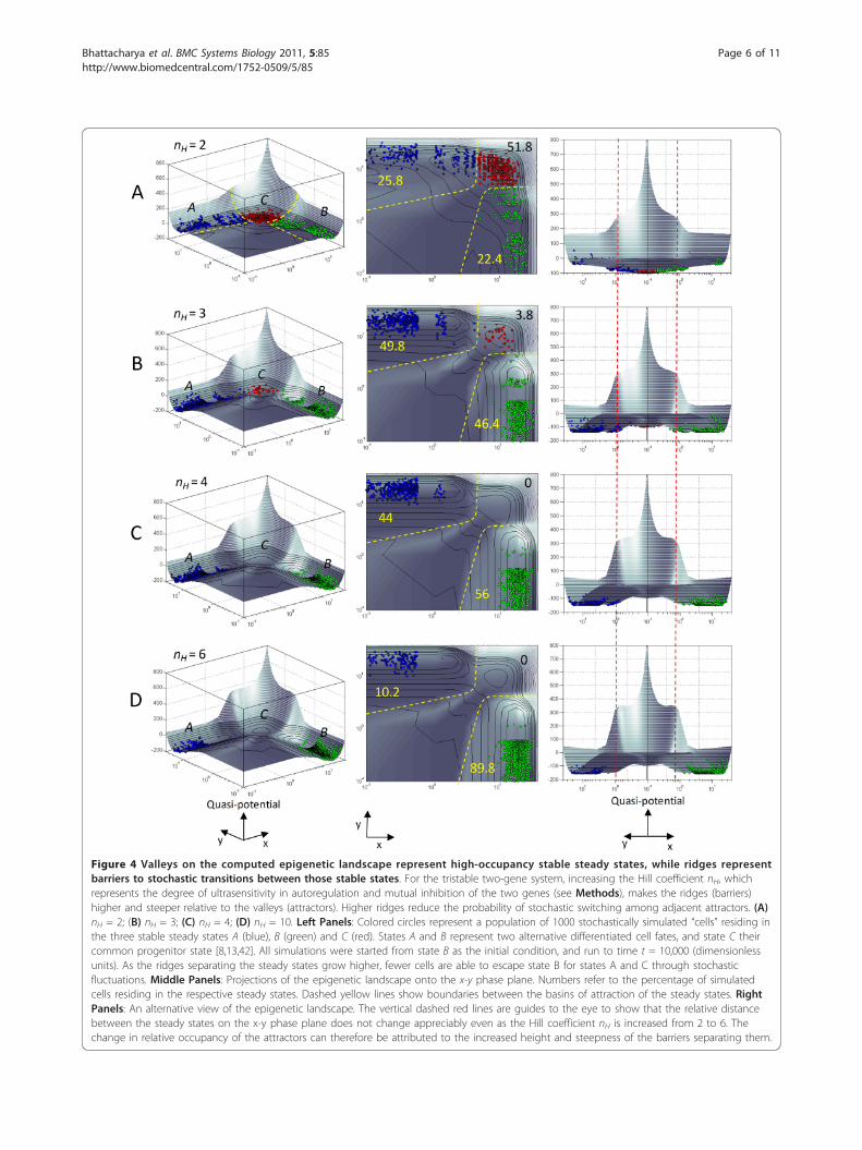
Figure 4 Valleys on the computed epigenetic landscape represent high-occupancy stable steady states, while ridges representbarriers to stochastic transitions between those stable states. For the tristable two-gene system, increasing the Hill coefficient nH, whichrepresents the degree of ultrasensitivity in autoregulation and mutual inhibition of the two genes (see Methods), makes the ridges (barriers)higher and steeper relative to the valleys (attractors). Higher ridges reduce the probability of stochastic switching among adjacent attractors. (A)nH = 2; (B) nH = 3; (C) nH = 4; (D) nH = 10. Left Panels: Colored circles represent a population of 1000 stochastically simulated “cells” residing inthe three stable steady states A (blue), B (green) and C (red). States A and B represent two alternative differentiated cell fates, and state C theircommon progenitor state [8,13,42]. All simulations were started from state B as the initial condition, and run to time t = 10,000 (dimensionlessunits). As the ridges separating the steady states grow higher, fewer cells are able to escape state B for states A and C through stochasticfluctuations. Middle Panels: Projections of the epigenetic landscape onto the x-y phase plane. Numbers refer to the percentage of simulatedcells residing in the respective steady states. Dashed yellow lines show boundaries between the basins of attraction of the steady states. RightPanels: An alternative view of the epigenetic landscape. The vertical dashed red lines are guides to the eye to show that the relative distancebetween the steady states on the x-y phase plane does not change appreciably even as the Hill coefficient nH is increased from 2 to 6. Thechange in relative occupancy of the attractors can therefore be attributed to the increased height and steepness of the barriers separating them.


Page 6 of 11

derived from the dynamic rate equations without anyadditional information, thus yields an interpretation ofcellular stability not immediately apparent from two-dimensional phase portrait analysis. The analysis abovesupports the contention that the length of the “leastaction trajectory” along the contours of the epigeneticlandscape is more important in predicting transitionsbetween alternative cellular states than the simple “aerialdistance” in state space [13]. It is also interesting to notethat the contours of the quantitatively mapped epige-netic landscape act as a constraint on the extent of sto-chastic fluctuations in protein levels, with simulatedcells “smeared out” on the surface of a shallower basin(Figure 4A, middle panel) compared to a tighter distri-bution of cells on a deeper valley (Figure 4D, middlepanel).These results suggest that calculating the relative

heights of the ridges and valleys on the computed epige-netic landscape of a multi-gene system can help predictthe probability of trans-differentiation from one celllineage to another, or de-differentiation of a particularcell type to its progenitor state. Current efforts to repro-gram cell fate with potential application in regenerative

medicine suffer from a low rate of successful reprogram-ming [36] and a trial-and-error approach to choice of areprogramming strategy [13]. Computing the epigeneticlandscape for the critical gene interactions regulatingthe transition between two cellular states may indicateparticular genetic manipulations that would lower thebarriers separating the two states, thereby increasing theefficiency of the reprogramming process. It can alsohelp characterize the relative ease or difficulty of alter-native routes of cell fate transition [7,9,36]. For instance,comparison of the elevation of the barriers separatingtwo terminally-differentiated cell lineages on the epige-netic landscape might suggest that de-differentiation ofcells of one lineage to the common progenitor cell ofthe two lineages followed by redirection to the secondlineage would lead to more efficient reprogrammingthan direct trans-differentiation (Figure S2, AdditionalFile 1).

A dynamic landscapeThe computed epigenetic landscape derived aboveshould not be interpreted as a static surface [45]. Altera-tions in gene interactions in course of development or

Figure 5 Height and steepness of barriers affects stochastic occupancy of stable states. (A) Percentage of stochastically simulated cells inthe three attractors A, B and C in the tristable two-gene system at time t = 10,000 for a range of values of the Hill coefficient nH. All simulationswere started from state B as the initial condition, and run to time t = 10,000 (dimensionless units). (B, C) With increasing nH, the height andsteepness of the ridges relative to the valleys is increased, making stochastic transitions (arrows) from state B to state C, and thereafter to state A,less likely. (At longer time scales, where the distribution of the cell population among various attractors approaches an equilibrium, the percentageof cells in each attractor correlates simply to the relative depth of the attractor: see Figure S1, Additional File 1.) (B) nH = 2; (C) nH = 6.


Page 7 of 11

experimental manipulation will change the shape of thelandscape, in turn altering the stability of individualsteady states or creating novel steady states. Forinstance, increasing the basal expression of one gene inthe tristable gene network sharply lowers the elevationof the corresponding attractor state relative to the otherattractors (Figure 6A, B). As a result, cells located in theshallower attractor are destabilized and “roll into” thevalley representing the deeper, more stable attractorstate. This may explain the phenomenon of trans-differ-entiation of cells of one lineage into another by forcedexpression of a gene regulating the second lineage or byconditional deletion of a gene required for the first line-age [29,30].Interestingly, this flexibility of the quasi-potential sur-

face under gene manipulation gives a quantitative inter-pretation of the revised image of the epigenetic landscapeproposed by Waddington (Figure S3, Additional File 1),which showed an array of pegs representing genes, hold-ing up a sheet of fabric (the landscape) through a net-work of guy ropes (gene interactions) - meant to conveythe idea that “the modelling of the epigenetic landscape... is controlled by the pull of these numerous guy-ropeswhich are ultimately anchored to the genes [5]“. Similarchanges in the shape of the epigenetic landscape mayalso be brought about by external signals - for exampleendogenous cytokines or environmental chemicals -which by transiently altering the landscape could have aninstructive effect on cell fate choice.

ConclusionsIn this work, we have defined a deterministic quasi-potential that is minimized along a temporal trajectoryfollowed by a gene network, and used it to quantitativelyderive the corresponding epigenetic landscape. A gene

network not being a mechanical system, this quasi-potential should not be confused with a potential energyfunction. It is rather a Liapunov function of the dynami-cal system represented by the gene network, alongwhich trajectories flow monotonically “downhill”towards the steady states of the network [41]. Otherinvestigators have used a term analogous to the quasi-potential difference Δ Vq in Eq. 4 to calculate the“energy landscape” for concentrations of one componentin a gene network [46,47]. Here we have used the con-cept of alignment of multiple trajectories to interpolatethe epigenetic landscape of a two-variable system.This novel and simple process for deriving the surface

of the landscape from a path-integral quasi-potential isnot restricted to two-gene systems. While the landscapecannot be visually rendered for circuits with more thantwo genes, the rates of transition across the potentialbarriers between multiple steady states in the systemcan still be computed to predict optimum routes of cellfate reprogramming.However, many binary branching points in develop-

ment, particularly in blood cell lineage specification, aregoverned by mutual antagonism of only two transcrip-tion factors associated with alternative lineage choices[37]. Mapping the epigenetic landscape of pairs of suchcross-inhibitory “master regulators” should therefore beof particular interest in understanding both normaldevelopment and induced cell fate reprogramming, andcan be greatly aided by detailed quantitative characteri-zation of the interactions between these regulators.

MethodsBistable network modelTo illustrate the derivation of the epigenetic landscape,we used a simplified mathematical model of a bistable

Figure 6 The shape of the computed epigenetic landscape can be altered by modifying gene interaction parameters. When basalexpression By of gene y in the tristable two-gene system (see Methods) is increased from By = 0 (A) to By = 4 (B) (dimensionless units),attractor A on the landscape is “lowered” relative to attractor B, causing cells to “roll into” the more stable state A from the destabilized state B.Numbers on the figure refer to the percentage of stochastically simulated cells in the respective attractors. All simulations were started fromstate B as the initial condition, and run to time t = 10,000. Hill coefficient nH = 10 in both figures.


Page 8 of 11

network of two genes, x and y, that suppress each otherto form a double-negative feedback loop. The dynamicsof the model are described by the two rate equations:

dxdt

= BX +foldYX · KnH

DYX

KnHDYX + ynH

− degX · x (6)

dydt

= BY +foldXY · KnH

DXY

KnHDXY + xnH

− degY · y (7)

where variables x and y represent the concentrationsof the two gene products, and parameters BX and BY

denote the basal (constitutive) expression rates of genesx and y, respectively. The parameters foldYX and foldXYrepresent the rate constants, and KDYX and KDXY theeffective affinity constants, for the suppressive effects ofgene y on gene x, and of gene x on gene y, respectively.The mutual suppression of the two genes is quantifiedby the Hill-coefficient nH (the interaction is ultrasensi-tive for values of nH > 1). Parameters degX and degYrepresent the first-order degradation rate constants forthe two gene products x and y, respectively. For thissimplified model we used dimensionless parameterswith the following values: foldYX = foldXY = 2; KDYX =0.7; KDXY = 0.5; BX = BY = 0.2; degX = degY = 1; nH = 4.These values were tuned to ensure bistable switchingbehavior in the model.

Tristable network modelThe tristable network model consisted of two genes, xand y, that in addition to mutual suppression, inducetheir own expression (positive autoregulation). Thedynamics of this model are described by:

dxdt

= BX +foldXX · xnH

KnHDXX + xnH

+foldYX · KnH

DYX

KnHDYX + ynH

− degX · x (8)

dydt

= BY +foldYY · ynH

KnHDYY + xnH

+foldXY · KnH

DXY

KnHDXY + xnH

− degY · y (9)

where the new parameters foldXX and foldYY representthe rate constants, and KDXX and KXYY the effective affi-nity constants, for the positive autoregulation of genes xand y, respectively. The default parameter values chosento ensure three robust stable states in this model wereas follows: foldXX = foldYY = foldYX = foldXY = 10; KDXX

= KDYY = KDYX = KDXY = 4; BX = BY = 0; degX = degY =1; nH = 4. This system has been modeled previously[42,48,49] in the context of mutual inhibition of thetranscription factors PU.1 and GATA1 in common mye-loid progenitor (CMP) cells, which gives rise to eitherbipotential granulocyte/macrophage progenitor (GMP)cells or megakaryocyte/erythroid progenitor (MEP) cells.

Integration AlgorithmTo evaluate the change in the quasi-potential along eachtrajectory in x-y phase space by numerical integration,the initial level of the quasi-potential at time t = 0 atthe origin of the trajectory was arbitrarily set to zero(the same initial quasi-potential level was used for alltrajectories so that the drop in the quasi-potential alongeach trajectory could be compared and used as a basisfor alignment of multiple trajectories along a basin ofattraction).Thereafter, at each time step:

• The ratesdxdt

anddydt

were updated to the current

value of x and y according to Eqs. 8 and 9.• Expression levels x and y were updated as:

xnew = xold + �x (10)

ynew = yold + �y (11)

where for increments in time Δt (fixed for a simula-tion to ensure convergence), the changes in x and y aregiven by:

�x =dxdt

· �t (12)

�y =dydt

· �t (13)

• The quasi-potential Vq was updated as:

Vqnew = Vq

old + �Vq (14)

where:

�Vq = −dxdt

· �x − dydt

· �y (15)

The above steps were repeated until the quasi-poten-tial Vq converged to a minimum (decided by a pre-settolerance). Multiple trajectories thus obtained werealigned into basins of attraction according to the processdescribed in the main text. The quasi-potential surfacewas then derived by linear interpolation among thealigned trajectories.

Software platforms usedThe deterministic models were implemented and simu-lated on the MATLAB® (R2009a, The MathWorks, Inc.,Natick, MA) platform, while the BioNetS program [50],based on the Gillespie algorithm [51,52], was used for


Page 9 of 11

stochastic simulations. All graphics were rendered onMATLAB®.

Visualization of stochastic simulation resultsThe stochastically simulated “cells” (i.e. individual reali-zations of the stochastic network model) were overlaidon the quasi-potential surface at the x and y values pre-dicted for each cell. Since stochastic simulations yieldintegral values, we added a small random “deviation”term [= (rand*0.5) where rand is a MATLAB® functionthat draws pseudorandom values from the standard uni-form distribution on the open interval (0,1)] to eachsimulated x and y value to visualize multiple cells situ-ated at the same point in x-y phase space. The appropri-ate “elevation” for each cell on the quasi-potentialsurface was calculated by linear interpolation betweenthe two points on the deterministic trajectories “closestto” the location of the cell in x-y phase space. Sourcecode for the model in MATLAB® format is appended inAdditional File 2.

Additional material

Additional file 1: Supplementary Figures. This file includes additionalfigures to supplement the text.

Additional file 2: Supplementary Model Code. This file lists the sourcecode in MATLAB®® format for the computational algorithm used toderive the epigenetic landscape.

AcknowledgementsWe thank J. D. Schroeter, C. Woods, R. B. Conolly, H. J. Clewell III, J.E. Trosko,M. Thattai, J. M. Haugh and B. Howell for critical discussions and reading ofthe manuscript. This work was supported by the Superfund ResearchProgram of the U.S. National Institute of Environmental Health Sciences, andby the American Chemistry Council.

Authors’ contributionsSB designed the study, constructed the computational model andperformed computer simulations, and wrote the paper. QZ participated instudy design. QZ and MEA discussed the results and commented on themanuscript. All authors read and approved the final manuscript.

Received: 17 February 2011 Accepted: 27 May 2011Published: 27 May 2011

References1. Gilbert S: Epigenetic landscaping: Waddington’s use of cell fate

bifurcation diagrams. Biology and Philosophy 1991, 6(2):135-154.2. Slack JMW: Conrad Hal Waddington: the last renaissance biologist? Nat

Rev Genet 2002, 3(11):889-895.3. Waddington CH: An introduction to modern genetics. London: George

Allen & Unwin; 1939.4. Waddington CH: Organisers and Genes. Cambridge, UK: Cambridge

University Press; 1940.5. Waddington CH: The Strategy of the Genes. London: George Allen &

Unwin; 1957.6. Kauffman SA: Metabolic Stability and Epigenesis in Randomly

Constructed Genetic Nets. J Theor Biol 1969, 22(3):437-467.7. Enver T, Pera M, Peterson C, Andrews PW: Stem Cell States, Fates, and the

Rules of Attraction. Cell Stem Cell 2009, 4(5):387-397.

8. Huang S: Reprogramming cell fates: reconciling rarity with robustness.Bioessays 2009, 31(5):546-560.

9. MacArthur BD, Ma’ayan A, Lemischka IR: Systems biology of stem cell fateand cellular reprogramming. Nat Rev Mol Cell Biol 2009, 10(10):672-681.

10. Thom R: Structural Stability and Morphogenesis. Reading, MA: W. A.Benjamin, Inc; 1976.

11. Thom R: An Inventory of Waddingtonian Concepts. In Theorical Biology:Epigenetic and Evolutionary Order from Complex Systems. Edited by: GoodwinB, Saunders P. Edinburgh: Edinburgh University Press; 1989:1-7.

12. Wang J, Xu L, Wang E, Huang S: The Potential Landscape of GeneticCircuits Imposes the Arrow of Time in Stem Cell Differentiation. Biophys J2010, 99(1):29-39.

13. Zhou JX, Huang S: Understanding gene circuits at cell-fate branch pointsfor rational cell reprogramming. Trends Genet 2011, 27(2):55-62.

14. Kim KY, Wang J: Potential energy landscape and robustness of a generegulatory network: Toggle switch. PLoS Comput Biol 2007, 3(3):565-577.

15. Cao Y, Liang J: Optimal enumeration of state space of finitely bufferedstochastic molecular networks and exact computation of steady statelandscape probability. BMC Syst Biol 2008, 2.

16. Zhu XM, Yin L, Hood L, Ao P: Robustness, stability and efficiency ofphage λ genetic switch: Dynamical structure analysis. J Bioinform ComputBiol 2004, 2(4):785-817.

17. Zhu XM, Yin L, Hood L, Ao P: Calculating biological behaviors of epigeneticstates in the phage λ life cycle. Funct Integr Genomics 2004, 4(3):188-195.

18. Lapidus S, Han B, Wang J: Intrinsic noise, dissipation cost, and robustnessof cellular networks: The underlying energy landscape of MAPK signaltransduction. Proc Natl Acad Sci USA 2008, 105(16):6039-6044.

19. Wang J, Xu L, Wang EK: Potential landscape and flux framework ofnonequilibrium networks: Robustness, dissipation, and coherence ofbiochemical oscillations. Proc Natl Acad Sci USA 2008, 105(34):12271-12276.

20. Li C, Wang E, Wang J: Potential Landscape and Probabilistic Flux of aPredator Prey Network. PLoS ONE 2011, 6(3):e17888.

21. Takahashi K, Yamanaka S: Induction of pluripotent stem cells from mouseembryonic and adult fibroblast cultures by defined factors. Cell 2006,126(4):663-676.

22. Takahashi K, Tanabe K, Ohnuki M, Narita M, Ichisaka T, Tomoda K,Yamanaka S: Induction of pluripotent stem cells from adult humanfibroblasts by defined factors. Cell 2007, 131(5):861-872.

23. Wernig M, Meissner A, Foreman R, Brambrink T, Ku MC, Hochedlinger K,Bernstein BE, Jaenisch R: In vitro reprogramming of fibroblasts into apluripotent ES-cell-like state. Nature 2007, 448(7151):318-U312.

24. Maherali N, Sridharan R, Xie W, Utikal J, Eminli S, Arnold K, Stadtfeld M,Yachechko R, Tchieu J, Jaenisch R, Plath K, Hochedlinger K: Directlyreprogrammed fibroblasts show global epigenetic remodeling andwidespread tissue contribution. Cell Stem Cell 2007, 1(1):55-70.

25. Yu JY, Vodyanik MA, Smuga-Otto K, Antosiewicz-Bourget J, Frane JL, Tian S,Nie J, Jonsdottir GA, Ruotti V, Stewart R, Slukvin II, Thomson JA: Inducedpluripotent stem cell lines derived from human somatic cells. Science2007, 318(5858):1917-1920.

26. Dimos JT, Rodolfa KT, Niakan KK, Weisenthal LM, Mitsumoto H, Chung W,Croft GF, Saphier G, Leibel R, Goland R, Wichterle H, Henderson CE,Eggan K: Induced pluripotent stem cells generated from patients withALS can be differentiated into motor neurons. Science 2008,321(5893):1218-1221.

27. Hanna J, Markoulaki S, Schorderet P, Carey BW, Beard C, Wernig M,Creyghton MP, Steine EJ, Cassady JP, Foreman R, Lengner CJ, Dausman JA,Jaenisch R: Direct reprogramming of terminally differentiated mature Blymphocytes to pluripotency. Cell 2008, 133(2):250-264.

28. Shen CN, Slack JMW, Tosh D: Molecular basis of transdifferentiation ofpancreas to liver. Nat Cell Biol 2000, 2(12):879-887.

29. Xie HF, Ye M, Feng R, Graf T: Stepwise reprogramming of B cells intomacrophages. Cell 2004, 117(5):663-676.

30. Cobaleda C, Jochum W, Busslinger M: Conversion of mature B cells into Tcells by dedifferentiation to uncommitted progenitors. Nature 2007,449(7161):473-477.

31. Zhou Q, Brown J, Kanarek A, Rajagopal J, Melton DA: In vivoreprogramming of adult pancreatic exocrine cells to beta-cells. Nature2008, 455(7213):627-U630.

32. Vierbuchen T, Ostermeier A, Pang ZP, Kokubu Y, Sudhof TC, Wernig M:Direct conversion of fibroblasts to functional neurons by defined factors.Nature 2010, 463(7284):1035-U1050.


Page 10 of 11

http://www.biomedcentral.com/content/supplementary/1752-0509-5-85-S1.DOC

http://www.biomedcentral.com/content/supplementary/1752-0509-5-85-S2.DOC

http://www.ncbi.nlm.nih.gov/pubmed/12415319?dopt=Abstract
















































33. Ieda M, Fu JD, Delgado-Olguin P, Vedantham V, Hayashi Y, Bruneau BG,Srivastava D: Direct Reprogramming of Fibroblasts into FunctionalCardiomyocytes by Defined Factors. Cell 2010, 142(3):375-386.

34. Tursun B, Patel T, Kratsios P, Hobert O: Direct conversion of C. elegansgerm cells into specific neuron types. Science 2011, 331(6015):304-308.

35. Zhou Q, Melton DA: Extreme Makeover: Converting One Cell intoAnother. Cell Stem Cell 2008, 3(4):382-388.

36. Yamanaka S: Elite and stochastic models for induced pluripotent stemcell generation. Nature 2009, 460(7251):49-52.

37. Graf T, Enver T: Forcing cells to change lineages. Nature 2009,462(7273):587-594.

38. Huang S: Non-genetic heterogeneity of cells in development: more thanjust noise. Development 2009, 136(23):3853-3862.

39. Hochedlinger K, Plath K: Epigenetic reprogramming and inducedpluripotency. Development 2009, 136(4):509-523.

40. Gardner TS, Cantor CR, Collins JJ: Construction of a genetic toggle switchin Escherichia coli. Nature 2000, 403(6767):339-342.

41. Strogatz S: Nonlinear Dynamics and Chaos: With Applications to Physics,Biology, Chemistry, and Engineering (Studies in Nonlinearity). Cambridge,MA: Perseus Books Group; 2001.

42. Huang S, Guo YP, May G, Enver T: Bifurcation dynamics in lineage-commitment in bipotent progenitor cells. Dev Biol 2007, 305(2):695-713.

43. Wilkinson DJ: Stochastic modelling for quantitative description ofheterogeneous biological systems. Nat Rev Genet 2009, 10(2):122-133.

44. Kaern M, Elston TC, Blake WJ, Collins JJ: Stochasticity in gene expression:From theories to phenotypes. Nat Rev Genet 2005, 6(6):451-464.

45. Roeder I, Radtke F: Stem cell biology meets systems biology. Development2009, 136(21):3525-3530.

46. Hasty J, Pradines J, Dolnik M, Collins JJ: Noise-based switches andamplifiers for gene expression. Proc Natl Acad Sci USA 2000,97(5):2075-2080.

47. Acar M, Becskei A, van Oudenaarden A: Enhancement of cellular memoryby reducing stochastic transitions. Nature 2005, 435(7039):228-232.

48. Roeder I, Glauche I: Towards an understanding of lineage specification inhematopoietic stem cells: A mathematical model for the interaction oftranscription factors GATA-1 and PU.1. J Theor Biol 2006, 241(4):852-865.

49. Chickarmane V, Enver T, Peterson C: Computational Modeling of theHematopoietic Erythroid-Myeloid Switch Reveals Insights intoCooperativity, Priming, and Irreversibility. PLoS Comput Biol 2009, 5(1):e1000268.

50. Adalsteinsson D, McMillen D, Elston TC: Biochemical Network StochasticSimulator (BioNetS): software for stochastic modeling of biochemicalnetworks. BMC Bioinformatics 2004, 5:24.

51. Gillespie DT: A general method for numerically simulating the stochastictime evolution of coupled chemical reactions. Journal of ComputationalPhysics 1976, 22(4):403-434.

52. Gillespie DT: Exact Stochastic Simulation of Coupled Chemical-Reactions.J Phys Chem 1977, 81(25):2340-2361.

doi:10.1186/1752-0509-5-85Cite this article as: Bhattacharya et al.: A deterministic map ofWaddington’s epigenetic landscape for cell fate specification. BMCSystems Biology 2011 5:85.

Submit your next manuscript to BioMed Centraland take full advantage of:

• Convenient online submission

• Thorough peer review

• No space constraints or color figure charges

• Immediate publication on acceptance

• Inclusion in PubMed, CAS, Scopus and Google Scholar

• Research which is freely available for redistribution

Submit your manuscript at www.biomedcentral.com/submit


Page 11 of 11




































A deterministic map of Waddington's epigenetic landscape for cell fate specification

Documents

Transcript of A deterministic map of Waddington's epigenetic landscape for cell fate specification