A conservative stabilized finite element method for the magneto-hydrodynamic equations

INTERNATIONAL JOURNAL FOR NUMERICAL METHODS IN FLUIDS

Int. J. Numer. Meth. Fluids 29: 535–554 (1999)

A CONSERVATIVE STABILIZED FINITE ELEMENTMETHOD FOR THE MAGNETO-HYDRODYNAMIC

EQUATIONS

NIZAR BEN SALAHa,b, AZZEDDINE SOULAIMANIb, WAGDI G. HABASHIa,* ANDMICHEL FORTINc

a CFD Laboratory, ER-301, Department of Mechanical Engineering, Concordia Uni6ersity,1455 de Maisonneu6e Bl6d. W., Montreal, Quebec H3G 1M8, Canada

b Ecole de technologie superieure, Departement de genie mecanique, Uni6ersite du Quebec, 1100 rue Notre-Dame Ouest,Montreal, Quebec H3C 1K3, Canada

c Departement de mathematiques et de statistique, Uni6ersite La6al, Ste-Foy, Quebec G1K 7P4, Canada

SUMMARY

This work presents a finite element solution of the 3D magneto-hydrodynamics equations. The formula-tion takes explicitly into account the local conservation of the magnetic field, giving rise to a conservativeformulation and introducing a new scalar variable. A stabilization technique is used in order to allowequal linear interpolation on tetrahedral elements of all the variables. Numerical tests are performed inorder to assess the stability and the accuracy of the resulting methods. The convergence rates arecalculated for different stabilization parameters. Well-known MHD benchmark tests are calculated.Results show good agreement with analytical solutions. Copyright © 1999 John Wiley & Sons, Ltd.

KEY WORDS: finite element method; MHD equations; conservative formulation; stabilization techniques; Hartmannflow; MHD Rayleigh flow; numerical solutions

1. INTRODUCTION

Numerical methods for magneto-hydrodynamic (MHD) equations have attracted the interestof many researchers over the past two decades. The literature presents mainly two trends forformulating MHD problems: using the magnetic field B as the independent variable or usingthe vector potential A with the associated scalar potential. Choosing between the twoformulations depends on many factors and, especially on the physical problem to be solved.The methods of solving for the vector potential are well-known in the pure electromagneticcontext [1–4]. One can consult Biro and Preis [5] for a general overview of the vector potentialmethods, and some of their electromagnetic applications.

In the context of MHD, these methods have also been popular and intensively used to solveMHD equations in different situations. Fautrelle [6] used a vector potential formulation insolving the magnetic part of electromagnetic stirring problems. He treated it as a pureelectromagnetic problem by dropping motion effects in the Maxwell equations. Mestel [7]examined, both analytically and numerically, the process of levitation melting of metals.

* Correspondence to: CFD Laboratory, Department of Mechanical Engineering, Concordia University, 1455 deMaisonneuve Blvd. W., ER-301, Montreal, Quebec H3G 1M8, Canada.

CCC 0271–2091/99/050535–20$17.50Copyright © 1999 John Wiley & Sons, Ltd.

Recei6ed July 1997Re6ised October 1997

N. BEN SALAH ET AL.536

Lympany et al. [8] presented numerical results for the MHD effects in aluminium reductioncells. Assuming a steady two-dimensional phenomenon, they solved for the scalar potential f

and deduced the magnetic field using the Biot–Savart law. Besson et al. [9] developed atwo-dimensional finite element method for solving both the MHD and the free-surfaceproblems associated with electromagnetic casting (EMC). They represented the outside poten-tial by an integral equation, so their method could be described as a FEM/BEM one. Morerecently, Conraths [10] described the magnetic field by an electric vector potential and amagnetic scalar potential, for modeling an inductive heating device for thin moving metalstrips. While this literature survey is by no means exhaustive, it illustrates the general use ofvector potential formulations, indicates their popularity and wide use in the literature andunderlines the main idea of these formulations: namely, that the introduction of the vectorpotential circumvents the explicit imposition of the magnetic free-divergence constraint sincethe conservation of the magnetic field is implicitly respected within the definition of the vectorpotential.

The second main trend in the literature consists in solving directly for the magnetic field B.Doing so would normally result in an overdetermined system of equations. This can beovercome by dropping the free-divergence equation and the terms implying this same diver-gence within the magnetic induction equation. The resulting vectorial equation is a diffusion–convection ‘Helmholtz’-like equation. Such a formulation has also been thoroughly used forthe solution of MHD equations. One can consult Sazhin et al. [11], where the authors solvedthe resulting Helmholtz equation with a finite difference method, or Gardner and Gardner[12], who presented a two-dimensional bi-cubic B-spline finite element method for the MHDchannel flow. Once again, while this literature survey of the ‘Helmholtz’ formulation is notmeant to be either exhaustive or complete, it indicates that these formulations have alreadybeen used by many authors and in many different contexts.

These two main families of formulations share a feature in common. Both do not explicitlyimpose the free-divergence condition on the magnetic field. To the best of the authorsknowledge, only Oki and Tanahashi [13,14] have developed numerical schemes that explicitlysatisfy the solenoidal condition of the magnetic field. They introduced a variable calledhydromagnetic cross-helicity G=u ·B and retained the free-divergence equation within theirsystem of equations. They presented results for the natural convection of a thermoelectricallyconducting fluid under a magnetic field. The actual work, initiated in [15], aimed at developinga conservative finite element method for the MHD equations. ‘Conservation’ means anappropriate satisfaction of the free-divergence condition by the numerical scheme. Therefore,in this paper a conservative and stable finite element solution of the 3D MHD equations ispresented, with a method that takes into account both the magnetic induction and themagnetic field conservation equations.

The remainder of the paper is organized in five sections. In the first section, the MHDgoverning equations are presented and reviewed. The above cited Helmholtz and vectorpotential formulations are presented and briefly commented upon. In the second section, theconservative method is developed. It will be shown that the introduction of a Lagrangemultiplier within the system of equations circumvents the overdetermination of the system,while giving rise to equivalent equations if appropriate boundary conditions are prescribed. Inthe third section, the Galerkin weak form of the equations is obtained, giving rise to a mixedfinite element formulation. A stabilization technique is introduced to circumvent the usualBrezzi–Babuska stability conditions and to allow equal interpolation for all the variables. It isalso seen that a penalty factor is introduced in order to force the magnetic divergence towardszero. In the fourth section, systematic numerical experiments are carried out to assess the

Copyright © 1999 John Wiley & Sons, Ltd. Int. J. Numer. Meth. Fluids 29: 535–554 (1999)

FE METHOD FOR THE MHD EQUATIONS 537

accuracy and stability of the different methods resulting from our formulation. Tests are thenrun to validate the numerical code that has been developed. The main conclusions aresummarized in the last section.

2. THE GOVERNING EQUATIONS

The MHD equations can be derived from the Maxwell equations, Ohm’s law for a movingmedium and the principle of conservation of the electric charge (Landau et al. [16]). Under theclassical assumptions of neglecting both the displacement current (D/(t and the time variationof the charge density (q/(t, when compared with the electric current density j (D and q are theelectric induction field and the electric charge density respectively), assuming the permittivitye, the magnetic permeability m and the electric conductivity s to be constants (e and m areequal to those of free space), one can write:

9×B=m j, (1)

9×E= −(B(t

, (2)

9 ·B=0, (3)

j=s(E+U×B), (4)

9 · j=0, (5)

where B and E are respectively, the magnetic and electric fields. Noting that by virtue of (1)the divergence of the electric current density j is zero, Equation (5) becomes superfluous.Taking the curl of Ohm’s law (4), term by term, and making use of Faraday’s and Ampere’slaws (1) and (2), one obtains:

(B(t

−9× (U×B)+h9× (9×B)=0, (6)

where h=1/ms, is the magnetic diffusivity coefficient. Once Equation (6) is solved for themagnetic field B, the electric field can be deduced from the following equation:

E=9×B

h−U×B (7)

and then the electric current density j can be calculated from Equation (4).Equation (6) is the best known and used form of the magnetic induction equation. It consists

of a diffusive second-order curl–curl term, a convective first-order curl term and a hyperbolicin time first-order term. It brings the advantage of directly relating the main hydrodynamicquantity, namely the velocity field, to the main electromagnetic one, namely the magnetic field,without any interference. Here it should be pointed out, that the magnetic free-divergenceconstraint (3), which was not used, is implicit in Equation (6). Indeed, if the divergence ofEquation (6) is taken, term by term, one obtains the following condition on the divergence ofB:

((9 ·B)(t

=0. (8)



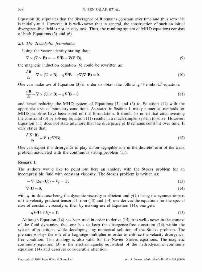
Equation (8) stipulates that the divergence of B remains constant over time and thus zero if itis initially null. However, it is well-known that in general, the construction of such an initialdivergence-free field is not an easy task. Thus, the resulting system of MHD equations consistsof both Equations (3) and (6).

2.1. The ‘Helmholtz’ formulation

Using the vector identity stating that:

9× (9×B)= −92B+9(9 ·B), (9)

the magnetic induction equation (6) could be rewritten as:

(B(t

−9× (U×B)−h92B+h9(9 ·B)=0. (10)

One can make use of Equation (3) in order to obtain the following ‘Helmholtz’ equation:

(B(t

−9× (U×B)−h92B=0 (11)

and hence reducing the MHD system of Equations (3) and (6) to Equation (11) with theappropriate set of boundary conditions. As stated in Section 1, many numerical methods forMHD problems have been based on this formulation. It should be noted that circumventingthe constraint (3) by solving Equation (11) results in a much simpler system to solve. However,Equation (11) does not state anymore that the divergence of B remains constant over time. Itonly states that:

((9 ·B)(t

=9 · (h92B). (12)

One can expect this divergence to play a non-negligible role in the discrete form of the weakproblem associated with the continuous strong problem (11).

Remark 1:

The authors would like to point out here an analogy with the Stokes problem for anincompressible fluid with constant viscosity. The Stokes problem is written as:

−9 · (2hg(U))+9p=F, (13)

9 ·U=0, (14)

with h, in this case being the dynamic viscosity coefficient and g(U) being the symmetric partof the velocity gradient tensor. If from (13) and (14) one derives the equations for the specialcase of constant viscosity h, then by making use of Equation (14), one gets:

−h92U+9p=F. (15)

Although Equation (14) has been used in order to derive (15), it is well-known in the contextof the fluid dynamics, that one has to keep the divergence-free constraint (14) within thesystem of equations, while developing any numerical solution of the Stokes problem. Thepressure p plays the role of a Lagrange multiplier in order to enforce the velocity divergence-free condition. This analogy is also valid for the Navier–Stokes equations. The magneticcontinuity equation (3) is the electromagnetic equivalent of the hydrodynamic continuityequation (14) and deserves considerable attention.



2.2. The 6ector potential formulation

Alternative to the above derivation of equations, one can start from Ohm’s law (4), makeuse of Equation (1), and noting that by definition:

E= −9f−(A(t

, (16)

write the following equation in terms of the vector potential A:

(A(t

−U× (9×A)+h9× (9×A)+9f=0, (17)

the vector potential A being defined as:

B=9×A. (18)

Introducing such a vector brings the advantage of implicitly respecting the divergence-freeconstraint (3). However, this technique of introducing the vector potential presents a challeng-ing problem when gauging the field A and dealing with its boundary conditions in order toenforce the uniqueness of the solution of the magnetic field.

3. THE CONSERVATIVE FORMULATION

In order to introduce this family of formulations, let us recall the ‘Helmholtz’ formulation. Theidea leading to this formulation is that the system composed of Equations (3) and (6) isoverspecified and leads to more equations than unknowns. For example, in the three-dimen-sional case and if the velocity field is assumed known, the system of equations composed byEquations (3) and (6), gives rise to four linear equations with three unknowns. In Jiang et al.[17], the authors showed that an equivalent situation exists in the pure electromagnetic context.They demonstrated that the first-order div–curl Maxwell’s system of equations (1)–(3) is notan overdetermined one. They showed that by introducing two dummy scalar variables, theyend up with an equivalent system of eight equations with eight unknowns. They underlined thedangers of circumventing the ‘overspecification’ of system (1)–(3) by dropping the free-diver-gence equation (3). These dangers are related to the ellipticity of the system, the uniqueness ofthe solution and the ensuing spurious numerical solutions that may appear.

Using the same technique, it will be shown that the second-order system of Equations (3)and (6) is not an overspecified one.

Let V be a bounded, simply connected, convex and open domain, which is included in R3,with a piecewise smooth boundary G, the union of G1 and G2, with n, the unity normaloutward vector. Let Equations (3) and (6) hold in the domain V and be associated withappropriate boundary conditions on G. Adding the gradient of a scalar variable to Equation(6), one gets the following new equation:

(B(t

−9× (U×B)+h9× (9×B)+9p=0 in V. (19)

Let the homogeneous Dirichlet condition

p=0 (20)



hold on the boundary G. Taking the divergence of Equation (19) and using Equation (3), onegets:

Dp=0 in V. (21)

As Equation (21) is submitted to the boundary condition (20), this leads to the uniquephysical solution p=0 over all the domain V. Thus, the scalar p is really a dummy variable(which in theory should be null) and the system of Equations (3) and (19) is equivalent to thesystem (3) and (6). The new system of equations has in the three-dimensional case, fourequations with four unknowns and is no longer overdetermined. By analogy to the Stokes andthe Navier–Stokes equations, p is interpreted as a Lagrange multiplier used to enforce thedivergence-free condition (3).

Remark 2:

Equation (19) could be rewritten in many equivalent forms. Particularly, after making use ofthe vector identity (9), one gets the following equivalent equation:

(B(t

−9× (U×B)−h92B+h9(9 ·B)+9p=0 in V. (22)

In the rest of the present work, Equation (22) along with the constraint (3), is used as themodel for the MHD equations.

Remark 3:

It is easily predictable that non-respect of the constraint (3) leads to inaccurate numericalsolutions. In order to show this, suppose one discards the divergence-free equation and retainsonly Equation (10). Let for simplicity, the velocity field be equal to zero, and assume theproblem to be steady. From (10), one obtains:

9× (9×B)=0 in V, (23)

with the most probable boundary conditions

n ·B=0 on G1, (24)

n×B=0 on G2. (25)

The solution of Equation (23) subject to the boundary conditions (24) and (25) is notunique. It admits a kernel composed of the gradient of scalar variables satisfying theconditions (24) and (25). Any numerical method for problem (23)–(25) will fail to provide aunique solution. The constraint (3) should thus be taken into account and it behaves like agauge condition filtering the divergence-free solution. The respect of this condition reduces thekernel of spurious solutions to a unique null scalar function.

Indeed, according to the unity partition theorem (Brezis [18]), there exist scalar functions f

that are C�, satisfying (f/(n=0 on G1, n×9f=0 on G2 and f=0 in a part of V. Thus, ifB0 is a particular solution of (23)–(25), then any vector B=B0+9f is also a solution. But ifthe vector solution has to satisfy the divergence-free condition, then Df=0 in V. As (f/(n=0on G1 and n×9f=0 on G2, then f is equal to a constant in V. Since f is prescribed zero ina part of the domain, then f=0 over all the domain V.



4. VARIATIONAL FORMULATION AND DISCRETIZATION

4.1. The Galerkin method

The Galerkin weighted residual formulation for the system of Equations (3) and (19) isobtained through multiplying the two equations by two test functions B* and p* respectively,chosen in two appropriate functional spaces. After integrating the resulting equations over thewhole domain V, one gets:&

VB*·

�(B(t�

dV−h&

VB*·92B dV+h

&V

B*·9(9 ·B) dV−&

VB*·9× (U×B) dV

+&

VB*·9p dV=0, (26)

&V

p*(9 ·B) dV=0, (27)

for all B* and all p*.Applying the divergence theorem, the weak form of the Galerkin formulation is obtained as:&

VB*·

�(B(t�

dV+h&

V9B*·9B dV−

&V

B*·9× (U×B) dV+&

VB*·9p dV

−h&

V(9 ·B)(9 ·B*) dV−h

&G

(n ·9B*)·B* dG+h&

G(n ·B*)(9 ·B) dG=0, (28)

&V

p*(9 ·B) dV=0. (29)

In the usual manner, the discrete problem associated with the weak form (28) and (29) can beestablished as:&

VBh*·

�(B(t�

dV+h&

V9Bh*·9Bh dV−

&V

Bh*·9× (U×Bh) dV+&

VBh*·9ph dV

−h&

V(9 ·Bh)(9 ·Bh*) dV−h

&G

(n ·9Bh) ·Bh* dG+h&

G(n ·Bh*)(9 ·Bh) dG=0, (30)

&V

ph*(9 ·Bh) dV=0, (31)

for all Bh* and ph* belonging to some finite-dimensional functional subspaces.The variational problem formulated by Equations (30) and (31) is of mixed type and

presents many similarities with the mixed variational formulation for the Navier–Stokesequations (Brezzi and Fortin [19]). Hence, it requires the respect of the inf–sup stabilitycondition, also called the L.B.B. condition in order to find a stable numerical solution(Bh*, ph*). In practice, the respect of this stability condition implies the use of differentapproximations for the two variables (Bh*, ph*). In three dimensions, elements respecting theL.B.B. condition could prove expensive with regard to execution time and memory storage.Moreover, the implementation of three dimensions mixed formulations is quite complicated.Another way of obtaining a stable finite element method for the system (30) and (31) is bycircumventing the L.B.B. condition (Hughes et al. [20]).



4.2. The stabilized finite element method

Suppose Vh=@Ve, a certain partition of the domain V into elements and h the ‘size’ of anelement Ve. Following Brezzi and Pitkaranta [21], the continuity equation (31) is modified as:&

Vph*(9 ·Bh) dV+ %

Ve�Vh

t1&

Ve

9ph ·9ph* dV=0, (32)

where t1 is a function of the mesh size h to be specified.This stabilization technique is equivalent to augmenting the continuity equation (3) of the

strong problem with a Laplacian dissipation term of the scalar p and has already been usedsuccessfully for the Navier–Stokes incompressible and compressible flows (Baruzzi et al. [22]).Hence, the stabilized formulation can be introduced as:&

VBh*·

�(B(t�

dV+h&

V9Bh*·9Bh dV−

&V

Bh*·9× (U×Bh) dV+&

VBh*·9ph dV

−h&

V(9 ·Bh)(9 ·Bh*) dV−h

&G


G(n ·Bh*)(9 ·Bh) dG=0, (33)

&V

ph*(9 ·Bh) dV+ %Ve�Vh

t1&

Ve

9ph ·9ph* dV=0. (34)

Once the stability of the formulation is insured, the volume integral emanating from the9(9 ·B) term is penalized with a term t2 in order to enforce the magnetic divergence towardsmall values when the convection is dominant (i.e. small values of h). Then, the implementedformulation could be presented as:&

VBh*·

�(B(t�

dV+h&

V9Bh*·9Bh dV−

&V

Bh*·9× (U×Bh) dV+&

VBh*·9ph dV

+ (t2−h)&

V(9 ·Bh)(9 ·Bh*) dV−h

&G


G(n ·Bh*)(9 ·Bh) dG=0,

(35)&V

ph*(9 ·Bh) dV+ %Ve�Vh

t1&

Ve

9ph ·9ph* dV=0. (36)

The stabilized method defined by (35) and (36) allows the use of equal interpolation for thetwo variables (Bh*, ph*), thus facilitating the implementation and permitting the use of cheaperelements. In this work, all the variables are interpolated by linear functions on tetrahedralelements.

5. NUMERICAL RESULTS

5.1. Steady case

In order to assess the stability and the quality of the finite element formulation describedabove, the problem (35)–(36) is studied in a cubic domain (05x51, 05y51, 05z51). Thevelocity vector is fixed to U= (1, 0, 0)T. The Dirichlet boundary conditions and the sollicita-tion vector f= (2x−2h, −2h, 2z)T are imposed in such a way as to reproduce approximatelyan arbitrary solution of the continuous problem, namely B= (x2, y2, −2(x+y)z)T and p=0.The dissipation coefficient t1 can be given by one or the other of the two following expressions:



t1=ah2

4h, (37)

t1=a��2 U

h�2

+�4h

h2

�2�−1/2

. (38)

The penalization factor t2 could be set to either t2=0, which corresponds to the originalphysical model, or to t2= U h/2. In the later case the coefficient r=t2−h ends up to be:

r=h�

1−Remh

2�

, (39)

where Remhis the local magnetic Reynolds number defined by:

Remh=sm U h. (40)

Computations have been made for two different magnetic diffusion coefficients h=1.2×10−1 and h=1.2×10−3 representing respectively, a highly diffusive case and a highlyconvective one, and for a=0.1, 1/3 and 1.0. For each case, the mesh variation of theL2(V)-norms of the magnetic divergence 9 ·Bh , the error Bh−B , the Lagrange multiplier ph and its gradient 9ph were all calculated.

Comments:

Highly con6ecti6e caseIf the magnetic convection is important (h=1.2×10−3), the best solutions are obtained witht2= U h/2 and this is true quite independently of the expression used for t1. Actually, themethods generated with t2= U h/2 are much more conservative and accurate than the‘Helmholtz’ formulation and the approximation obtained with t2=0 (Figure 1(a) and (b)).

However it should be noticed that the expression for t1 given in (38), which in this case isof order O(h) in the convective-dominant case, gives rise to optimal convergence rates for bothBh and ph. In fact, for the Lagrange multiplier p error and the magnetic field error, theconvergence rate is 2. For the gradient of ph and the divergence of Bh, the rates are aroundunity (Figure 2).

When t1 is fixed to its expression in Equation (37), which in the convective-dominant caseis of order O(h2), the convergence rates are still optimal for the magnetic induction field andfor its divergence, while for p and its gradient the rates become suboptimal. For ph, the rateis around 1 and the gradient of ph seems to be bounded by a constant. Figure 3 shows theseconvergence rates for a=0.1.

When compared together, the method generated by Equation (38) gives rise to betteraccuracy and magnetic conservation than the method generated by Equation (37). Themethods do not seem to be very sensitive to the value of the constant a, so a=0.1, seems asuitable value to be assigned.

If t2=0 and the convection is still dominant, then the accuracy of the method is very poorand the error norms are very important, especially when Equation (37) is used for t1.Regardless of the expression t1 used, the method is very sensitive to the value of the constanta showing signs of instabilities due to the effect of the convection. No general trend for theconvergence rates could be drawn. Thus, one should avoid using such a method.

Highly diffusi6e caseWhen diffusion is dominant (h=1.2×10−1), all the methods obtained by the differentexpressions of t1 and t2 are accurate, convergent and stable. When t2=0, both expressions



(37) and (38) for t1 give rise to approximately the same results in terms of error and magneticdivergence. This could be explained by the fact that since the magnetic diffusion is dominant,Equations (37) and (38) lead both to expressions of O(h2).

Figure 1. (a) The L2 norms of the magnetic field divergence vs. the mesh size. Comparison between the Helmholtzformulation and conservative formulation with: t1=0.1((2 U /h)2+ (4h/h2)2)−0.5; t2= U h/2; h=1.2×10−3. (b)The L2 norms of the magnetic field divergence vs. the mesh size. Comparison between the Helmholtz formulation and

conservative formulation with: t1=0.1((2 U /h)2+ (4h/h2)2)−0.5; t2= U h/2; h=1.2×10−3.



Figure 2. Different L2 norms vs. the mesh size; conservative formulation with t1=1.0((2 U /h)2+ (4h/h2)2)−0.5;t2= U h/2; h=1.2×10−3.

The convergence rates, obtained for the two expressions of t1 are the same. Convergencerates of 1 were obtained for the magnetic field divergence and for the scalar p. Theconvergence rate for the magnetic induction is of order 2 and the gradient of p is bounded bya constant (Figure 4). As expected, the linear interpolation on tetrahedral elements keeps theoptimal convergence rates for the magnetic induction and its gradient, while p and its gradientconvergence at suboptimal rates.

When t2= U h/2, the best results were obtained in terms of the error on Bh and on itsdivergence. However, the differences between these results and those obtained with t2=0 arenot very important. Again the convergence rates are those expected, optimal for the magneticfield and suboptimal for the scalar p (Figure 5). Once more, the results obtained are quiteindependent of t1 and of the constant a.

5.2. Unsteady case

In order to highlight the advantages of using the conservative stable formulation (35)–(36)rather than a formulation derived from the ‘Helmholtz’ equation (11), one should look at thebehavior of the solutions obtained with the two methods, for an unsteady problem, andcompare them in terms of the norm of the divergence of the magnetic field. In the same



manner as in Section 5.1, the velocity vector U= (1, 0, 0)T, the sollicitation force vectorf= (2x−2h+1, −2h, 2z)T and the Dirichlet boundary conditions are imposed in such a wayas to reproduce approximately an arbitrary unsteady solution of the continuous problemB= (x2+ t, y2, −2(x+y)z)T and p=0. Computations have been made with the followingcoefficients: t1=1.0h2/4h, t2= U h/2 and h=1.2×10−1.

Figures 6 and 7 show the evolution of the divergence of the magnetic field as a function ofthe time steps. In Figure 6, the first 50 time steps are highlighted, while in Figure 7 the numberof time steps is set to 1000. It is seen that the conservative formulation performs much betterthan the ‘Helmholtz’ formulation. It reaches an ‘optimal’ value after a few time steps, then italmost keeps on that same divergence (in reality the norm of the divergence keeps onreducing). With the ‘Helmholtz’ formulation, the divergence first increases then is reduced toa constant plateau that is approximately five times higher than the one obtained with theconservative formulation.

5.3. The Hartmann–Poiseuille flow

The Hartmann flow is one of the cornerstone examples of the MHD flows (Moreau [23]).The validation of any MHD code should use this flow as a benchmark test. Suppose a liquidmetal flowing under the influence of a pressure gradient, in the x-direction, through a

Figure 3. Different L2 norms vs. the mesh size; conservative formulation with t1=0.1(h2/4h); t2= U h/2; h=1.2×10−3.



Figure 4. Different L2 norms vs. the mesh size; conservative formulation with t1=0.1(h2/4h); t2=0; h=1.2×10−1.

rectangular cross-section duct that is infinitely long in the z-direction. Suppose a uniformexternal magnetic field B0 is applied along the y-direction. The liquid flow induces aperturbation of the imposed magnetic field B0, that is in the same x-direction as the flow.Assuming that the walls are at y=9L and are perfectly insulating, using the non-slipboundary conditions for the velocity and assuming the perturbation of the magnetic field to bezero at these walls, the problem has an analytical solution for the velocity and the magneticfield, that can be put in the following form:

Ux= −rGHagsB0

2

�cosh(Ha)−cosh(yHa/L)sinh Ha

�, (41)

Bx= −B0Rem

Ha�sinh(yHa/L)− (y/L) sinh(Ha)

cosh(Ha)−1�

, (42)

where Bx and Ux are respectively, the x-components of the magnetic and the velocity fields, rGthe pressure gradient keeping the fluid in motion (r being the density) and Rem and Ha are themagnetic Reynolds number and the Hartmann number respectively, defined as:

Rem=smUL, (43)



Ha=B0L� s

rn

�1/2

. (44)

The square of the Hartmann number is the ratio between the electromagnetic forces and theviscous forces. In Equation (43), U is the velocity Ux at y=0 and n is the kinematic viscosityof the liquid metal.

The Hartmann flow with the velocity field given as an input data, has been computed for thefollowing physical parameters: s=7.14×105 (V m)−1, h=1.2×10−1 m2 s−1, rn=1.5×10−4 kg m−1 s−1, rG=4.85×10−5 Pa m−1, L=0.5 m, B0=1.4494×10−4 Tesla. Theresults obtained from the analytical solution are compared with the results from the numericalcomputations. The agreement between the two is quite good (Figure 8). Then a parametricstudy is made using the Hartmann number as a parameter (Ha=1, 2, 5, 10, 20) (Figure 9).This parametric study shows a very good agreement with the analytical solution. Furthermore,this study puts into evidence the building of the Hartmann layer.

Figure 10 shows the analytical solution for the velocity (Ha=1, 2, 5, 10, 20). It is seen thatthe intensity of the applied transversal magnetic field influences the velocity field. From aPoiseuille profile when the magnetic field is zero (Ha=0), the velocity is flattened and becomesquite constant in the core region of the duct, with the gradient of the velocity concentrated intwo boundary layers (Hartmann layer) near the walls, when the magnetic field is strong(Ha�1). The flattening of the velocity profile is due to the magnetic braking of the flow. In

Figure 5. Different L2 norms vs. the mesh size; conservative formulation with t1=0.1(h2/4h); t2= U h/2; h=1.2×10−1.



Figure 6. The L2 norms of the magnetic field divergence vs. the time steps number. Comparison between theHelmholtz formulation and the conservative formulation with: t1=0.1(h2/4h); t2= U h/2; h=1.2×10−1.

Figure 7. The L2 norms of the magnetic field divergence vs. the time steps number. Comparison between theHelmholtz formulation and the conservative formulation with: t1=0.1(h2/4h); t2= U h/2; h=1.2×10−1.



Figure 8. The induced magnetic field along the y-axis; Ha=3.45, Rem=0.0916.

Figure 9, one can see the magnetic signature of this boundary layer and as the Hartmannnumber is increased from 1 to 20, one can see a boundary layer type behavior developing forthe induced magnetic field (Figure 9).

Figure 9. The induced adimensionalized magnetic field B* along the adimensionalized co-ordinate Y* (B*=BxB0/mrGL, Y*=y/L).



Figure 10. The x-component of the velocity along the y-axis.

Figure 11. The evolution of the induced magnetic field a vs. the co-ordinate y for different times t ; comparisonbetween analytical and numerical solutions.



Figure 12. The evolution of the velocity u vs. the co-ordinate y for different times t ; the analytical solution.

This behavior can be put into evidence because the walls are perfectly insulating, whichallows the use of the Dirichlet conditions for the magnetic field. If the walls were perfectlyconducting then the boundary conditions should be set to the Neumann-type conditions andhence the magnetic signature of the Hartmann layer would disappear.

5.4. The MHD Rayleigh flow

Suppose an infinite plane plate is at rest in a semi-infinite domain that is electricallyconducting. Let B0=0 be an applied magnetic field along y, the co-ordinate normal to theplate. Suppose the plate is suddenly set in motion at t=0, with a constant velocity U. Then,the motion propagates within the fluid domain as a wave. Ahead of this diffusive wave front,the fluid is still at rest; before the front, the fluid is in motion. Within the moving fluid, onecan distinguish two regions: The Hartmann layer in the vicinity of the plane plate, which hasa characteristic thickness d= (rn/s)1/2/B0, and a second region that is essentially a uniformplateau where the velocity is maximum and constant. The development of such a velocity fieldinduces a perturbation in the imposed magnetic field. This perturbation travels as a planewave. This wave is called the Alfven wave and travels within the fluid domain with a constantvelocity A0=B0/(mr)1/2. When the kinematic viscosity of the fluid is equal to its magneticdiffusivity, then the magnetic Prandlt number is equal to one (Prm=n/h), and an analyticalsolution exists for the MHD Rayleigh problem (Moreau [23]).

This analytical solution could be written in the following form:

u=U4

(2− (erfl+ +erfl−)+e−A0y/d (1−erfl−)+eA0y/d (1−erfl+)), (45)

a=U4

((erfl− −erfl+)+e−A0y/d (1−erfl−)−eA0y/d (1−erfl+)), (46)



where

l9=y9A0t2(dt)1/2 , (47)

d=n=h, (48)

a=b

(mr)1/2 , (49)

and u and b are the x-components of the velocity field and the induced magnetic fieldrespectively. This MHD Rayleigh problem, with the velocity space field given as an input data,has been computed with the following physical parameters: s= (107/(4p)) (V m)−1, h= l.0m2 s−1, r=0.4×10−4 kg m−1 s−1, B0=1.4494×10−4 Tesla and for t50.08 s. The resultsobtained from the analytical solution and the numerical computations are compared. Theagreement between the two is quite perfect (Figure 11). The three regions (Hartmann layer, themagnetic plateau and the wave front) are clearly distinguished. Figure 12 shows the corre-sponding analytical solution of the velocity field u(y, t).

6. CONCLUSIONS

A stabilized conservative finite element method for the 3D MHD equations is proposed. It isseen that the stability and the convergence of the method depends on the expressions of thecoefficients t1 and t2. The method has been validated through steady and unsteady tests. Themethod was then used for computing the Hartmann flow through a duct and the MHDRayleigh flow around a moving plane plate. The results are seen to be in a very goodagreement with the analytical solutions.

For industrial scale problems, the convection of the magnetic field is negligible whencompared with its diffusion. Hence, if t2=0 and t1=h2/4h, one obtains a method that isstable, accurate and quite simple. Moreover, since the conservation law is solved within thesystem, this method is more conservative regarding the norm of the magnetic field divergencethan the ‘Helmholtz’ formulation.

At astrophysical scales when convection is much more important than diffusion, t2= U h/2 and t1= ((2 U /h)2+ (4h/h2)2)−1/2 are more appropriate expressions to be used in order togenerate a stable and convergent formulation. Furthermore, these parameters generate meth-ods that are more conservative than the ‘Helmholtz’ formulation, and the difference betweenthe divergence norms calculated for the two methods are quite important.

When the MHD phenomenon to be studied is an unsteady one, then the advantages of usingthe conservative method with the appropriate coefficients are obvious. While the conservativemethod keeps on reducing the divergence of the vector solution, the ‘Helmholtz’ formulationgives rise to solutions that are much less accurate.

REFERENCES

1. M. Gyimesi and J.D. Lavers J.D., ‘Generalized potential formulations for magnetostatic problems’, IEEE Trans.Magn., 28, 1924–1929 (1992).

2. O.C. Zienkiewicz, J. Lyness and D.R.J. Owen, ‘Three-dimensional magnetic field determination using a scalarpotential, a finite element solution’, IEEE Trans. Magn., 13, 1649–1656 (1977).

3. V. K. Garg and J. Weiss, ‘Finite element solution of transient eddy current problems in multiply exited magneticsystems’, IEEE Trans. Magn., 22, 1257–1259 (1986).



4. S.C. Tandon and V.K. Chari, ‘Transient solution of the diffusion equation by the finite element method’, J. Appl.Phys., 52, 2431–2432 (1981).

5. O. Biro and K. Preis, ‘On the use of magnetic vector potential in the finite element analysis of three-dimensionaleddy currents’, IEEE Trans. Magn., 25, 3145–3159 (1989).

6. Y.R. Fautrelle, ‘Analytical and numerical aspects of electromagnetic stirring induced by alternating magneticfields’, J. Fluid Mech., 102, 405–430 (1981).

7. A.J. Mestel, ‘Magnetic levitation of liquid metals’, J. Fluid Mechs., 117, 27–43 (1982).8. S.D. Lympany, J.W. Evans and R. Moreau, ‘Magneto-hydrodynamic effects in aluminium reduction cells;

metallurgical applications of magneto-hydrodynamics, in H.K. Moffat and M.R.E. Proctor (eds.), Proc. Symp.Int. Union of The Theoritical and Applied Mechanics, Cambridge, UK (September 6–10, 1982), The Metals Society,London, 1984, pp. 15–23.

9. O. Besson, J. Bourgeois, P.A. Chevalier, J. Rappaz and R. Touzani, ‘Numerical modelling of electromagneticcasting processes’, J. Comp. Phys., 92, 482–507 (1991).

10. H.J. Conraths, ‘Eddy current and temperature simulation in thin moving metal strips’, Int. J. Numer. MethodsEng., 39, 141–163 (1996).

11. S.S. Sazhin, M. Makhlouf and T. Ishii, ‘Solutions of magneto-hydrodynamic problems based on a conventionalcomputational fluid dynamics code’, Int. J. Numer. Methods Fluids, 21, 433–442 (1995).

12. L.T.R. Gardner and G.A. Gardner, ‘A two-dimensional bicubic and B-spline finite element: used in a study ofMHD duct flow’, Comp. Methods Appl. Mech. Eng., 124, 365–375 (1995).

13. T. Tanahashi and Y. Oki, ‘Numerical analysis of natural convection of thermo-electrically conducting fluids in asquare cavity under a uniform magnetic field’, JSME Int. J., 38, 374–381 (1995).

14. T. Tanahashi and Y. Oki, ‘Numerical analysis of natural convection of thermo-electrically conducting fluids in asquare cavity under a uniform magnetic field (calculated results, frequency characteristics)’, JSME Int. J., 39,508–516 (1996).

15. N. Ben Salah, A. Soulaımani, W.G. Habashi and M. Fortin, ‘A conservative stabilized finite element method forthe magneto-hydrodynamic equations, in S.N. Atluri and G. Yagawa (eds.), Ad6ances in Computational Engineer-ing Science, International Computational Engineering and Science 97, Tech Science Press, Forsyth, GA, 1997, pp.269–276.

16. L.D. Landau, E.M. Lifshitz and L.P. Pitaevskii, Electrodynamics of Continuous Media, Pergamon, Oxford, 1984.17. B. Jiang, J. Wu and L.A. Povinelli, ‘The origin of spurious solutions in computational electromagnetics’,

NASA-TM-106921, E-9633, ICOMP-95-8, 1995.18. H. Brezis, Analyse Fonctionnelle, Theorie et Applications; Collection Mathematiques Appliquees pour la Maıtrise

sous la Direction de P.G. Ciarlet et J.L. Lions, Masson, Paris, 1983.19. F. Brezzi and M. Fortin, Mixed and Hybrid Finite Element Methods, Springer Series in Computational

Mathematics vol. 15, Springer, Berlin, 1991.20. T. Hugues, L. Franca and M. Ballestra, ‘A new finite element formulation for computational fluid dynamics: V.

Circumventing the Babuska–Brezzi condition: a stable Petrov–Galerkin formulation of the Stokes problemaccommodating equal-order interpolations’, Comp. Methods Appl. Mech. Eng., 59, 85–99 (1986).

21. F. Brezzi and J. Pitkaranta, ‘On the stabilization of finite element approximations of the Stokes problem’, in W.Hackbusch (ed.), Efficient Solutions of Elliptic Systems, Vieweg Notes on Numerical Fluid Mechanics, vol. 10,Vieweg, Wiesbaden, 1984, pp. 11–19.

22. G.S. Baruzzi, W.G. Habashi and M.M. Hafez, ‘A second-order finite element method for the solution of thetransonic Euler and Navier–Stokes equations’, Int. J. Numer. Methods Fluids, 20, 671–693 (1995).

23. R. Moreau, Magneto-hydrodynamics, Kluwer, Dordrecht, 1990.


A conservative stabilized finite element method for the magneto-hydrodynamic equations

Documents

Transcript of A conservative stabilized finite element method for the magneto-hydrodynamic equations