Behavior Research Methods, Instruments, & Computers2001, 33 (4), 443-456

The diffusion process has become quite popular in cog-nitive psychology during the last two decades (Hanes &Schall, 1996;Luce, 1986;Ratcliff, 1978;Ratcliff& Rouder,1998; Ratcliff, Van Zandt, & McKoon, 1999). In the studyof complicated stochastic models such as the diffusionprocess, simulationsof the model play an importantpart forthree reasons; they enable one to (1) understand the basiccharacteristics of the model, (2) generate data in order toevaluate estimation techniques for the model parameters,and (3) derive predictions to test the performance of themodel.

The problemwith simulating the diffusion process is thatit is a stochastic process with a continuous state and timespace. Roughly, we can distinguish two classes of simula-tion methods on the basis of accuracy of approximationofthe continuous diffusion process. First, there are methods

in which a discretization of the continuous state and/ortime space of the diffusionmodel is needed. In a secondclassof methods, no discretization is made, and the accuracy ofthe approximationof the continuousstate and time space islimited only by the precision of the floating-point imple-mentation. A method from the second class is expected togive always more exact results than any method from thefirst class. Therefore, it can be used as a benchmark to eval-uate the accuracy of methods from the first class.

Apart from differences in accuracy, simulationmethodsmay also differ with respect to their simulation speed. If ahuge number of simulationsof the model is needed, as, forinstance, in Markov chain Monte Carlo applications (Tan-ner, 1996), speed becomes an important issue.

The aim of this paper is to present an overview and eval-uation of techniques to simulate the diffusion process withconstant drift rate and variance, and two absorbing bound-aries (Cox & Miller, 1970). Such a process is also called aWiener process with absorbing boundaries,or a Brownianmotion with drift rate and absorbingboundaries. Hence, ifwe speakof a diffusionprocess,we mean theWienerprocess.In a separate section,we will indicate whether or not, and ifso, how the proposed simulationmethods can be adapted tosimulate other types of diffusion processes, but our majorfocus is on the Wiener process.

443 Copyright 2001 Psychonomic Society, Inc.

The first author was a research assistant of the Fund for Scientific Re-search (Flanders). The research in this paper was also supportedby BOFGrant GOA/02/2000 from the University of Leuven. We thank the edi-tor and two anonymous reviewers for their comments and suggestions.Address all correspondence to F. Tuerlinckx, Department of Statistics,Columbia University, 2990 Broadway MC 4403, New York, NY 10027(e-mail: tuerlinckx@neyman.stat.columbia.edu).

A comparison of four methodsfor simulating the diffusion process

FRANCIS TUERLINCKXUniversity of Leuven, Leuven, Belgium

ERIC MARISUniversity of Nijmegen, Nijmegen, the Netherlands

ROGER RATCLIFFNorthwestern University, Evanston, Illinois

and

PAUL DE BOECKUniversity of Leuven, Leuven, Belgium

Four methods for the simulation of the Wiener process with constant drift and varianceare described.These four methods are (1) approximating the diffusion process by a random walk with very small timesteps; (2) drawing directly from the joint density of responses and reaction time by means of a (possi-bly) repeated application of a rejection algorithm; (3) using a discrete approximation to the stochasticdifferential equation describing the diffusion process; and (4) a probability integral transform methodapproximating the inverseof the cumulativedistribution function of the diffusion process.The fourmeth-ods for simulating response probabilities and response times are compared on two criteria: simulationspeed and accuracy of the simulation. It is concluded that the rejection-based and probability integraltransform method perform best on both criteria, and that the stochastic differential approximation isworst. An important drawback of the rejectionmethod is that it is applicable only to the Wiener process,whereas the probability integral transform method is more general.

444 TUERLINCKX, MARIS, RATCLIFF, AND DE BOECK

Four methods for simulating the diffusion process arestudied here. The first method, used most commonly, isbased on the approximation of the diffusion process by arandom walk. The second method is built on a rejection al-gorithm for drawing directly from the first-passage timedensities of the diffusion process. The third method isbased on simulating a stochastic differential equationcharacterizing the diffusion process. The fourth methoduses the probability integral transform.

Thesemethodshavebeendescribed inotherplacesbefore.The theory for the first method is described in almost anytextbookon stochasticmodels (e.g., Feller, 1968). The refer-ence to the second method (Lichters, Fricke, & Schnaken-berg, 1995), however, is not readily accessible to psychol-ogists. Moreover, the method is described only for the casewith zero drift rate, and as a consequence, it is not directlyapplicable to the most common diffusion process used inpsychology. We therefore present an elaboratedand adaptedversion of the original algorithm.The third method can bederived in a straightforward manner from the definitionofthe diffusion process and is elaborated in, for instance,Bouleau and Lépingle (1994) and Fahrmeir (1976) (thesereferences contain only information about the case withoutabsorbing boundaries).The fourth method can be found inalmost any textbookon statistics (see, e.g., Mood, Graybill,& Boes, 1974).

The structure of the remainder of this paper is as fol-lows. First, a short overview is given of the type of diffu-sion process that is considered here. Second, the four sim-ulationmethodswill be presented.Third, thesemethodswillbe evaluated with respect to speed and accuracy of simu-lation. Fourth, the generality of the methods will be dis-cussed, and finally, some conclusionswill be presented.

OVERVIEW OF THE DIFFUSION PROCESS

In this section, we provide a brief overview of the basicfeatures of the diffusion process and introduce some nota-tion. A more technical and complete description of themodel and its mathematical properties can be found inspecializedreferences such as Coxand Miller (1970),Karlinand Taylor (1981), or Ross (1996).

The diffusion process is a stochastic process that de-velops through time, and it can be represented by a con-tinuous random variable X(t) (t � 0), denoting the positionof the process in the state space at time t(t � 0; t is alsocontinuous). In case of a diffusion process with absorbingboundaries 0 and a, the state space is restricted to the in-terval [0, a]. The central part of a stochastic process is thetransition probabilitydensity functionp(x0, t0; x, t), whichis the density for X(t) = x given that the process was at timepoint t0 (t0 < t) at position x0 and that the process did notreach one of the boundaries by time t.

Assume that the diffusion process starts at z (0 < z < a)at time 0. The transition probability density function p(z,0; x, t) should then satisfy the Kolmogorovequations,alsocalled the forward and backward differential equations

(Cox & Miller, 1970). Derivations of the Kolmogorovequations are presented in Cox and Miller and in Ross(1996), and their method of solution is explained in Coxand Miller. The forward equation is

(1)

which has to be solved for p(z, 0; x, t) subject to the con-ditions

(2)

The first condition is an initial value condition, whichmeans that, at time 0, all mass of the transition probabilitydensity function is concentratedat the starting point z. Thefunction d(x z) is the Dirac delta function, a degenerateprobabilitydensity with all its mass concentrated at 0. Thelast two conditionsare boundaryconditions,which imposethe restriction that the density equals zero at the boundaries,so that terminated processes disappear from the transitiondensity. The stochastic process described by Equations 1and 2 is called a diffusion process with constant drift rate,constant variance, and absorbing boundaries, or a Wienerprocess with absorbing boundaries. Since the exact formof the transitionprobabilitydensity function is not neededin this paper, it will not be presented here.

The parameters m and s2 are the infinitesimalmean andvariance of the process: m is the mean displacement ands 2 the variance of the displacement of X(t) given thatX(t t) = x, where t approaches to 0. The parameter m iscalled the drift rate of the diffusion process.

Two important events and corresponding random vari-ables originating from the diffusion process {X(t); t � 0}are of particular interest for simulating the diffusionprocess in the context of psychological research. First,there is the event that absorption occurs at the upperboundary. A random variable Y takes the value 1 if absorp-tion occurs at the upper boundary and value 0 if absorp-tion occurs at the lower boundary. The second importantevent is [T £ t |Y = 1], which is the event that the absorp-tion time T is smaller than some value t, given that ab-sorption happens in the upper boundary. We will consideralso the event [T £ t |Y = 0].

In psychological applications, it is impossible to ob-serve the full sample path {X(t); t � 0} from start until ab-sorption. Only the boundaryof absorption (i.e., the choiceresponse) and the time that it takes until absorption (i.e.,the choice response time) are observed. Therefore, it is notrequired that a simulation algorithm return a completesample path. Thus, for the simulation,we focus on the ran-dom variables Y and [T £ t |Y = 1].

Next, the density functions for the random variables de-fined above will be given. First, the probability of hittingthe upper boundary equals

p z x x z

p z a t

p z t

( , ; , ) ( )

( , ; , )

( , ; , ) .

0 0

0 0

0 0 0

= -==

d

12

0 0 022

2s m¶

¶- ¶

¶= ¶

¶p z x t

x

p z x t

x

z x t

t

( , ; , ) ( , ; , ) ( , ; , ),

p

SIMULATING THE DIFFUSION PROCESS 445

(3)

From the fact that the probability of absorption is a sureevent, it follows that Pr(Y = 0) equals 1 - Pr(Y = 1). Theprobability of hitting the lower boundary can also be ob-tainedfrom Equation3 by replacingmby -m and z by (a - z).This operation interchanges the role of the two absorbingboundaries but yields an otherwise identical diffusionprocess.

For the random variable T, we will not consider theprobability Pr(T £ t |Y = 1), but only present the condi-tional densityof first-passage times at the upper boundary:

(4)

where f(t |Y = 1) is defined for all t > 0. The other condi-tional density of first-passage times, f (t |Y = 0), can be ob-tained from Equation 4 by replacing m by - m and z by(a - z).

Typically, the diffusion process is applied to data froma two-alternative forced choice (2AFC) paradigm. How-ever, the response time that is observed consistsof more thanjust the decision time. It is often assumed that two com-ponents contribute to the response time: one that involvesthe decisionprocess, which can be modeledby the diffusionprocess, and another that involves all the other processes(encoding, response preparation, and execution). A com-plete model for response times in a 2AFC paradigm shouldalso take into account the second component. For sim-plicity, it is often assumed that all processes that are unre-lated to the decision process consume a constant time Ter.If this constant time is added to the decision times, thetotal response time RT becomes

RT = T + Ter. (5)

Under the assumption of a constant Ter, Equation 4 can beeasily adapted: In particular, t should be replaced by thedifference (t - Ter). Equation 3 does not change, of course.

If we would make the more realistic approach that Ter isa random variable (see, e.g., Ratcliff & Tuerlinckx,2001),then there are no explicit formulas for the conditionalden-sities, not even for simple choices of densities for Ter (e.g.,uniform, normal, or exponential).However, once we havea simulation method for the diffusion process, the simula-tion of a model with a random Ter poses no additionalprob-lems. For simplicity, in the remainder of the paper it willbe assumed that Ter is 0.

In some applications of the diffusion process (Ratcliff,1978; Ratcliff et al., 1999), it is assumed that the drift ratem and the starting point z show some trial-to-trial variabil-ity. The trial-to-trial variability is needed to limit accuracy(otherwise it grows toward 1 if boundary separation in-creases) and to fit the error response times (Ratcliff &Rouder, 1998).The simulation of such a process can be ac-complishedby drawing the drift rate and starting point fromthe appropriate distributions and then simulating the dif-fusion process with the drawn values. In the following,wewill assume that m and z are both constant, unless speci-fied otherwise.

FOUR METHODS FOR SIMULATINGTHE DIFFUSION PROCESS

In this section, the four methods are explained and analgorithm for each of them is outlined.

A Random Walk ApproximationIn many texts on stochastic processes, the diffusion

process with constant drift rate and absorbing boundariesis considered as the continuous version of the randomwalk process with absorbing states (see, e.g.,Cox & Miller,1970; Feller, 1968). The diffusion process can be derivedmathematically by constructing a random walk with verysmall displacements and small time intervals and by let-ting the length of both steps and time intervals approachzero. This limiting property is useful for the simulation ofthe diffusion process. In particular, it shows that a simu-lation from the diffusion process can be obtained by sim-ulating a random walk with small time intervals and dis-placements.

Assume a random walk with state space {0, D, 2D, . . . ,z - D, z, z + D, . . . , a}, in which 0 and a are the absorbingstates and z is the starting point. At every time interval t,a change occurs: a displacement D with probability p anda displacement-D with probabilityq = 1 - p. Assume fur-thermore that the following equalities hold:

(6)Under these conditions, if t converges to zero, the randomwalk converges to a diffusion process with drift rate m andvariance s2. From a given triplet (m, s, t), a triplet (p, q, D)can be computed from Equation 6, and a random walk ap-proximation is easily obtained.

The accuracy of the algorithm depends on the value oft, which will be denoted as precision in the following. If tis large, the approximationof the diffusion model will notbe very accurate, but the simulation will be fast. On theother hand, if t is small, the discrete approximation of the

p

q

= +æ

èçö

ø÷

= -æ

èçö

ø÷

=

12

1

12

1

m ts

m ts

s tD .

f t Y

a

a zt

Y

mm a z

am

at

T Y

m

| ( | )

exp( )

Pr( )

sin( )

exp ,

=

= - -æ

èç

ö

ø÷ =

´ -æèç

öø÷

-æèç

öø÷=

¥

å

1

2

11

12

2

2 2

2

2

2 2 2

21

ps ms

ms

p p s

Pr( )

exp

exp

Y = =-

æèç

öø÷

-

-æèç

öø÷

-1

21

21

2

2

z

a

ms

ms

446 TUERLINCKX, MARIS, RATCLIFF, AND DE BOECK

concrete process will be accurate, but the simulation timemay take too long to be of practical interest. A good valuefor t should return an accurate approximationand the sim-ulation should not take too much time.

To investigate how the simulation time depends on thevalue of t, results from the theory of the random walk canbe used. For a random walk with time interval t and statespace {0, D, 2D, . . . ,z - D, z, z + D, . . . , a}, the expectednumber of steps before absorption, E(N), in either of theboundaries is equal to (Feller, 1968)

With the use of the equalityD = sÖt, it is easy to show thatfor the case m = 0, if t is divided by a factor K, E(N) is mul-tiplied by the same factor K. Stated differently, E(N ) is oforder O(t 1). If m ¹ 0, this is more difficult to prove, butit can easily be checked numerically. These results showthat if the simulation is more accurate, it is also expectedto take more time.

To summarize: In the random walk approximation, thecontinuous time line is divided into small time intervals,and the position of the process at each time point is simu-lated. The magnitudeof the displacement D of the processis a monotonic increasing function of magnitude of thetime intervals (D = sÖt ). Thus, smaller time intervals leadto smaller displacements.A drawback of the random walkapproximation is that the expected simulation time in-creases with the accuracy of the approximation.

A Rejection-Based AlgorithmThe second method differs from the first in that there is

no attempt to simulate the sample path {X(t); t � 0}. In-

stead, the second method directly simulates the time thatit would take for the process to travel a fixed distance Rfrom its starting point.This ideawas developedby Lichterset al. (1995). They described an algorithm for the zerodrift rate case, and this algorithm will be extended here tothe case in which m can take any real value.

The algorithm of Lichters et al. (1995) makes use of arejection algorithm for simulating a symmetric diffusionprocess (i.e., z = a/2) with absorbingboundaries.With thisalgorithm, it is possible to obtain an exact draw from thefirst-passage density, given absorptionat one of the bound-aries. This rejection algorithm is then used as a compo-nent of a more general algorithm for the simulation froman asymmetric diffusion process (z ¹ a/2).

The algorithm to simulate a diffusion process will bedescribed in two parts. First, we will discuss the rejectionalgorithmfor the symmetric diffusion process. Second, wewill give an outline of a simulation algorithm for the moregeneral asymmetric case.

Part 1: Rejection Method for the SymmetricWiener Process

In the special case of a symmetric Wiener process, theconditional response time density in Equation 4 simpli-fies remarkably. See Equation 8 below.

Thus, for a symmetric Wiener process, the conditionalfirst-passage time distributions are the same. This equa-tion can be simplified further by noting that

(9)

where d is a positive integer. Equation 8 can now berewritten as seen in Equation 10 below.

For Equation 10, it is shown in AppendixA that the fol-lowing inequality holds:

(11)f t Y M tT Y| ( | ) exp( )= £ -1 l l

sin

,

p mm d

m d

m d2

1 1 4

0 2

1 3 4

æ

èçö

ø÷=

= +

=

- = +

ì

íïï

îïï

if

if

if

E N

z

q p

a

q p

qp

qp

z a z

z

a( )

.

( )= --

-´

-æèç

öø÷

-æèç

öø÷

¹

-æè

öø

=

ì

í

ïïïï

î

ïïïï

D D

D D D

D

D

1

1

0

0

7

if

if

m

m

(8)

(10)

f t Ya

a at

nn

at

T Y

n

n

| ( | ) exp exp exp

( )( ) exp( )

.

= =æèç

öø÷

+ -æèç

öø÷

é

ëê -

æ

èç

ö

ø÷

´ + - - +æ

èç

ö

ø÷

=

¥

å

12 2 2

2 1 1 12

2 1

2

2 2 2

2

2

2 2 2

20

ps ms

ms

ms

p s

f t Y f t Ya

a a

t m m m

at

T Y T Y

m

| |( | ) ( | ) exp exp

exp sin exp .

= = = =æèç

öø÷

+ -æèç

öø÷

é

ëê

´ -æ

èç

ö

ø÷

æ

èçö

ø÷-

æèç

öø÷=

¥

å

1 02 2

2 212

2

2 2 2

2

2

2 2 2

21

ps ms

ms

ms

p p s

SIMULATING THE DIFFUSION PROCESS 447

where

(12)

and

(13)

Since the inequality in Equation 11 holds for any t, it maybe used for a rejection algorithm for simulating fromfT |Y (t |Y = 0) or fT |Y (t |Y = 1). The rejection algorithm isexplained in AppendixB (see also Press, Flannery, Teukol-sky, & Vetterling, 1986; Tanner, 1996).

In the sampling algorithm for a symmetric diffusionprocess, it is first decided whether a realization fromfT |Y (t |Y = 1) or fT |Y(t |Y = 0) has to be simulated. Next, arealization is drawn from fT |Y (t |Y = 1) or fT |Y (t |Y = 0),dependent on the value for Y. Assume for simplicity thatthe outcome of the first step of the algorithm is 1 (i.e., Y =1). However, notice that the algorithm is the same for thecase Y = 0, since fT |Y(t |Y = 1) = fT |Y (t |Y = 0).

A rejection algorithm is initiated by sampling from acandidate-generating distribution. In our case, this is theexponentialdistributionwithparameterlasdefined in Equa-

tion 13. Sampling a realization t* from an exponentialdis-tribution involves the following computation:

(14)

where u is a uniform random number from U(0,1) and lis defined as in Equation 13. The draw t* from the expo-nential distribution is a candidate draw from fT |Y(t |Y = 1)and is accepted as a draw from that distribution if

(15)

where v is another random number from U(0, 1), and M isdefined as in Equation 12. After some rewriting, the con-dition in Equation 15 becomes

(16)

where

.

Convergence of the infinite sum in Equation 16 is fast.The number of terms will typicallybe lower than 15. Con-vergence is worst if u is close to zero.

Since the presented algorithm is a rejection algorithm,the acceptance rate is equal to 1/M. The acceptance rate is

Fa

=+

p sp s m

2 4

2 4 2 2.

v u n uF n F n

n

£ + - + - -- +

=

¥

å1 1 2 1 1 1 2 1

1

2

( ) ( )( ) ( ) ,( )

vf t Y

M t

T Y£=

-| ( * | )

exp( *)

1

l l

t u* | ln( ) |= - -1 1l

l ms

p s= +æ

èçö

ø÷2

2

2 2

22 2a.

M a

a a

a

=

æèç

öø÷

+ -æèç

öø÷

é

ëê

+æ

èç

ö

ø÷

ps ms

ms

ms

p s

2

2 2 2

2

2

2 2

2

2 2

2 2

exp exp

Figure 1. The acceptance rate as a function of drift rate for three values of a. The solid line repre-sents the case a = 0.16; the dashed line, a = 0.12; and the dotted line, a = 0.08 (s = 0.1).

448 TUERLINCKX, MARIS, RATCLIFF, AND DE BOECK

not constant, since M is a function of m, a, z, and s 2 (seeEquation 12). If m = 0, then the acceptance rate equalsp/4 = 0.785, and for m ¹ 0, it will be always lower thanp/4. In Figure 1, the acceptance rate as a function of driftrate m (on the abscissa) is shown for three different valuesof a (s is always equal to 0.1). Both the range of m and thedifferent values of a are realistic values, in the sense thatone may encounter them in real applications(given that s =0.1); they produce decision times around 1 sec. It can beseen that in the most extreme case in Figure 1 (a = 0.16and m = 0.4), the overall acceptance rate is still about 0.3.

In conclusion, a symmetric diffusion process can besimulated very easily in two steps: (1) Determine theboundary of absorption, based on the probabilities ofreaching each of the boundaries; and (2) draw a responsetime from the conditionalresponse time density, given theboundary of absorption.

Part 2: Rejection-Based Method for the GeneralWiener Process

We now proceed with the general Wiener process, with-out the requirement of a starting point symmetrically be-tween the absorbingboundaries.The rejection method de-scribed in the previous subsection will be applied one ormore times in order to obtain a realization from the moregeneral process. In particular, given the starting point, anew diffusion process is defined with symmetric absorb-ingboundaries that lie between the originalboundaries,andthe rejection method is applied. If the simulated value islocated at one of the original absorbing boundaries, theprocess stops, and if not, again a new symmetric diffusionprocess is defined, and this goes on until absorption oc-curs at one of the originalboundaries.Each time a fixeddis-tance is traveled (the distance in the symmetric diffusionprocess from the starting point to the absorbing boundary)and howlong it takes to travel the fixeddistance is simulated.

The central property of the diffusion process on whichthe algorithm is based is the Markov property: Once it isdetermined that the process is at a certain state, x(t) at timet, the future behaviorof the process does not dependon howstate x(t) was reached.

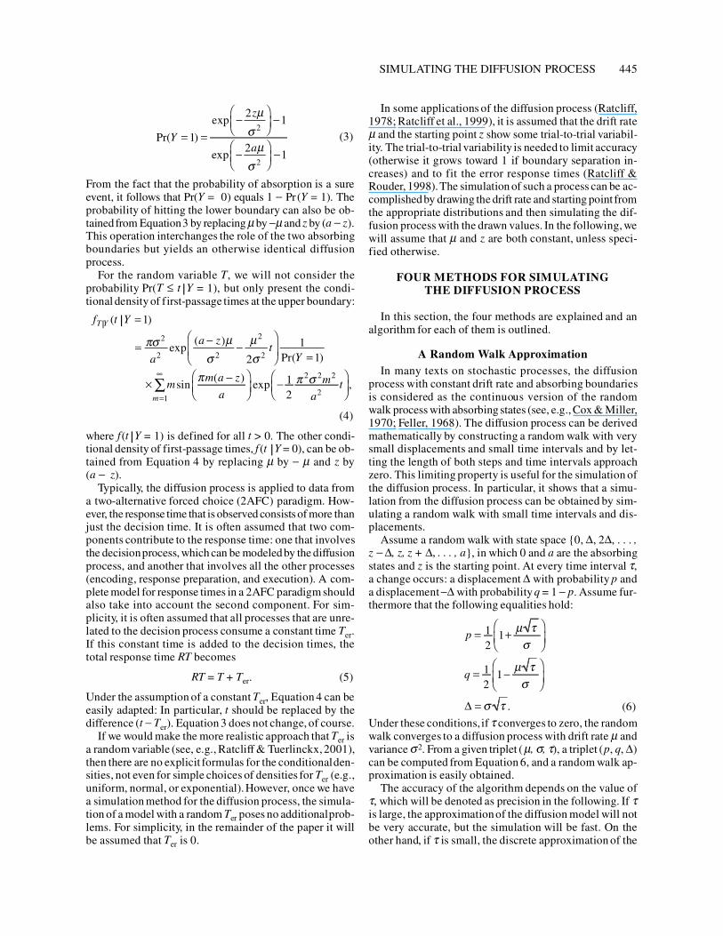
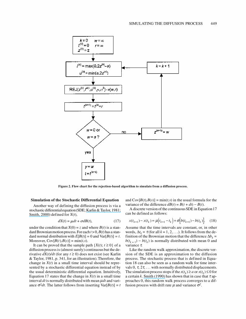
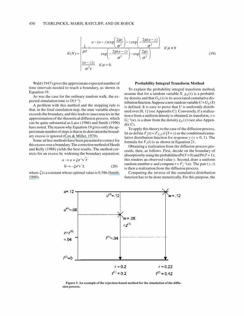
The algorithm is explained further in detail on basis ofa flow chart (Figure 2) and an example (Figure 3). First,the variables of the algorithm are initialized. The integerk is a counter, t(0) is the simulated time at step 0, and z(0) isthe starting point of the first symmetric diffusion process.At the start of the algorithm, z(0) equals z, the starting pointof the original diffusion process. In the example in Figure 3,the absorbing boundaries of the general diffusion processare 0 and 0.12, and the starting point is 0.04. Therefore,the starting point of the first symmetric diffusion processis also 0.04. The other two variables, w and r, are positionand time variables. They will be assigned values in thecourse of the algorithm.

Next, a new diffusion process with the starting point ex-actly in between the two absorbing boundaries is defined.

The starting point has already been initialized, and thelower and upper boundary (l(k) and u(k)) are now chosen sothat one of them equals an absorbingboundaryof the orig-inal diffusion process, in particular the absorbing boundaryclosest to the new starting point.The drift rate and varianceremain unchanged. In the example, the absorbing bound-aries of the originaldiffusion process are 0 and 0.12.There-fore, with starting point at 0.04, the new absorbing bound-aries for step 0 are 0 (the most nearby original absorbingboundary) and 0.08. Notice that the starting point 0.04 liesexactly halfway between these boundaries.New absorbingboundaries are represented by a dotted line in Figure 3.

In a third step, the rejection algorithmas described in theprevious subsection is applied to the new symmetrical dif-fusion process. In the flow chart, the rejection algorithm isdenotedby REJ, and the outcome of the simulationassignsvalues to w and r. The position w must equal l(k) or u(k).After this, the total simulation time is updated. In the ex-ample, the first application of the rejection algorithm re-sults in w = 0.08 and r = 0.20 and the observation is de-noted by “x” in Figure 3.

If the simulation of the symmetrical diffusion processleads to an absorption at one of the boundariesof the orig-inaldiffusionprocess, then the simulationstops. In that case,the final boundary of absorption is known, as is the totalsimulated first-passage time. However, if absorption oc-curs at the other boundary, the rejection algorithm will beappliedanother time but with the new starting pointw, thecurrent position in the state space. In the example, the re-jection algorithm has to be applied another time, since wis not equal to 0.0. The new starting point, z(1), is nowequal to 0.08, and the new absorbing boundaries are 0.04(dotted line) and 0.12. The second application of the re-jection algorithm ends up in the upper boundary of theoriginal diffusion process, so that the algorithmstops. Thesimulated time in this step was 0.22, so that the total sim-ulated diffusion time is equal to 0.42.

The advantage of the rejection-basedmethod is that thesimulation time is not proportional any more to the phys-ical time to run through the process. Another advantageover the random walk method is that it does not involve adiscrete approximationto the continuousdiffusion process.Therefore, the accuracy of the simulation is bounded onlyby the numerical accuracyof the computersystem on whichthe simulation takes place.

It is difficult to obtain theoretical results about the sim-ulation time for the rejection-based algorithm in Figure 2.The simulation time depends on the acceptance rate forthe input parameter values and the number of times thatthe absorbing boundaries of the original diffusion processdo not coincide with the chosen boundaries from the re-jection algorithm. However, both the acceptance rate andthe expected number of times that a subdivision of theoriginal diffusion process in a symmetric subprocess hasto be made depend on so many things that it is difficult tomake general assertions.

SIMULATING THE DIFFUSION PROCESS 449

Simulation of the Stochastic Differential EquationAnother way of defining the diffusion process is via a

stochasticdifferentialequation(SDE; Karlin & Taylor, 1981;Smith, 2000) defined for X(t),

dX(t) = mdt + sdB(t), (17)

under the condition that X(0) = z and where B(t) is a stan-dard Brownianmotionprocess.For each t > 0, B(t) has a stan-dard normal distribution with E[B(t)] = 0 and Var[B(t)] = t.Moreover, Cov[B(t ),B(s)] = min(t,s).

It can be proved that the sample path {X(t); t � 0} of adiffusion process is (almost surely) continuousbut the de-rivative dX(t)/dt (for any t � 0) does not exist (see Karlin& Taylor, 1981, p. 341, for an illustration).Therefore, thechange in X(t) in a small time interval should be repre-sented by a stochastic differential equation instead of bythe usual deterministic differential equation. Intuitively,Equation 17 states that the change in X(t) in a small timeinterval dt is normally distributedwith mean mdt and vari-ance s2dt. The latter follows from inserting Var[B(t)] = t

and Cov[B(t),B(s)] = min(t,s) in the usual formula for thevariance of the difference dB(t) = B(t + dt) - B(t).

A discrete version of the continuousSDE in Equation17can be defined as follows:

(18)

Assume that the time intervals are constant, or, in otherwords, Dtk = t (for all k = 1, 2, . . .). It follows from the de-finition of the Brownian motion that the difference Dbk =b(tk + 1) - b(tk ) is normally distributed with mean 0 andvariance t.

Like the random walk approximation, the discrete ver-sion of the SDE is an approximation to the diffusionprocess. The stochastic process that is defined in Equa-tion 18 can also be seen as a random walk for time inter-vals 0, t, 2t, . . . with normally distributed displacements.The simulationprocess stops if the x(tk ) � a or x(tk ) £ 0 fora certain k. Smith (1990) has shown that in case that t ap-proaches 0, this random walk process converges to a dif-fusion process with drift rate m and variance s2.

x t x t t t b t b tk k k k k k( ) ( ) ( ) ( ) .+ + +- = -( ) + -[ ]1 1 1m s

Figure 2. Flow chart for the rejection-based algorithm to simulate from a diffusion process.

450 TUERLINCKX, MARIS, RATCLIFF, AND DE BOECK

Wald (1947) gives the approximateexpected number oftime intervals needed to reach a boundary, as shown inEquation 19.

As was the case for the ordinary random walk, the ex-pected simulation time is O(t -1).

A problem with this method and the stopping rule isthat, in the final simulation step, the state variable alwaysexceeds the boundary, and this leads to inaccuracies in theapproximation of the theoretical diffusion process, whichcan be quite substantial as Luce (1986) and Smith (1990)have noted.The reason why Equation19 gives only the ap-proximatenumberof steps is that in its derivationthe bound-ary excess is ignored (Cox & Miller, 1970).

Some ad hoc methodshave been presented to correct forthisexcess overa boundary.The correctionmethodof Heathand Kelly (1988) yields the best results. The method cor-rects for an excess by widening the boundary separation:

a ® a + zs Ït0® -zsÏt, (20)

where z is a constant whose optimal value is 0.586 (Smith,1990).

Probability Integral Transform Method

To explain the probability integral transform method,assume that for a random variable X, gX (x) is a probabil-ity density and that GX (x) is its associated cumulative dis-tributionfunction.Supposea newrandomvariableU= GX (X)is defined. It is easy to prove that U is uniformly distrib-uted over [0, 1] (see Appendix C). Conversely, if a realiza-tion u from a uniform density is obtained, its transform, x =Gx

1(u), is a draw from the density gX (x) (see also Appen-dix C).

To apply this theory to the case of the diffusion process,let us define Fy(t) = FT |Y (t |Y = y) as the conditionalcumu-lative distribution function for response y (y = 0, 1). Theformula for F1(t) is as shown in Equation 21.

Obtaining a realization from the diffusion process pro-ceeds, then, as follows. First, decide on the boundary ofabsorptionby using the probabilitiesPr(Y = 0) and Pr(Y = 1);this renders an observed value y. Second, draw a uniformrandom number u and compute t = Fy

1(u). The pair (y, t)is then a realization from the diffusion process.

Computing the inverse of the cumulative distributionfunction has to be done numerically. For this purpose, the

Figure 3. An example of the rejection-based method for the simulation of the diffu-sion process.

E N

a a zz

za z

a z z

a z z

( )

( )exp exp( )

exp( )

exp

( ).

�´

- -æèç

öø÷

- - -æèç

öø÷

- -æèç

öø÷

-æèç

öø÷

¹

- =

ì

í

ïïï

î

ïïï

1

2 2

2 20

0

2 2

2 2

2

mt

ms

ms

ms

ms

m

s tm

if

if

(19)

SIMULATING THE DIFFUSION PROCESS 451

function Fy(t) can be approximated by using a grid ofpoints (nodes). Denote the sequence of N grid points byt1,. . .,tN. For each grid point ti, the corresponding functionvalue hi = Fy(ti) is calculated.A uniformly distributed ran-dom variable u is drawn and the associated realization t isdetermined as follows:

(22)

If N is taken large enough, the approximationwill be highlyaccurate. More complex approximations are also possible,such as linear interpolationbetween two grid points.

EVALUATION OF THESIMULATION METHODS

In this section, a Monte Carlo study is presented to eval-uate and compare the three simulationmethods on two cri-teria: speed and accuracy. The speed of the random walkand SDE approximations depends on the precision para-meter t. If a high precision is used (a small value of t), a lotof small simulationsteps may be needed,and that will slowdown the methods. Likewise, the speed of the probabilityintegral transform method depends on the number of tab-ulated grid points,N. For the probability integral transformmethod, setting up the table with function values can be alarge cost, but once that table is available, a value is easilydetermined. On the other hand, the speed of the rejection-based method depends on the amount of time that it takesto evaluateEquation16. These considerationsshow that itis difficult to make predictions about which method willbe faster.

Concerning accuracy, some firm statements can bemade, since the rejection-based method is an exact simu-lation method and hence is by definition better than everyapproximation method; therefore it functions as a bench-mark (it is needed to evaluate the accuracyof the three othermethods). It is interesting, however, to compare the per-formance of the three other methods with the performanceof the rejection-based algorithm. In particular, we are in-terested in the precision that is needed for the other meth-ods to be almost as accurate as the rejection-basedmethod.

To avoid superfluous notation, we will abbreviate thenames of the three simulation methods. The random walkapproximation will be denoted as the RW method, the

rejection-based method as the RB method, the stochasticdifferential equation approximation as the SDE method,and the probability integral transform method as the PITmethod.

Design and ProcedureThree independent variables are manipulated in the

Monte Carlo experiment: drift rate (m), combination ofboundary separation and starting point (a |z), and, if usedby the algorithm, the precision t. First, there are five levelsfor the drift rate m: 0.0, 0.1, 0.2, 0.3, and 0.4.Second, six lev-els for the combination of absorbing boundary and start-ing point are chosen (denoted as a |z): 0.08 |0.04,0.12 |0.06, 0.16|0.08,0.08|0.02,0.12|0.04, and 0.16|0.04.Third, three levels of precision t are chosen for the RW andSDE methods: 0.01,0.001,and 0.0001(ordered from low tohigh precision). For the PIT method, three levels of preci-sion are chosen (operationalized in number of gridpoints): 500, 5,000, and 50,000.

The three independentvariablesare completelycrossed.For each cell of the design, 20 samples of 3,000 observa-tions are simulated. All four methods are programmed inFORTRAN, and the Monte Carlo experiment is run on apersonal computer with a Pentium III 600-MHz processor.

For each criterion, speed and accuracy, we examine twodependent variables. First, with respect to speed, we com-pute the time that it takes to draw 3,000 observations.Sec-ond, the mean number of steps taken for the RW and SDEmethods to reach an absorbing barrier is computed, and,for the RB method, the mean number of applications ofthe rejection algorithm before an absorbing barrier isreached. For the PIT method, no steps have to be taken inthe simulation.

With respect to the accuracy of the simulation,again twodependent variables are examined. Both response proba-bility and the conditional response time density are simu-lated, and hence for both aspects the accuracy of approxi-mation is evaluated. First, we examine the proportion oftimes that the process hits the upper boundary. Second, forthe processes that hit the upper boundary, a measure ofmaximal deviation between the observed and theoreticalconditionalcumulative distribution function is computed:

(23)

where F̂1(t) is the empirical distribution function for thesimulatedvalues from the diffusion process, and F1(t) is the

H F t F tt

= -< <¥sup | ˆ ( ) ( ) |,

01 1

t

t u F t

t F t u F t i N

t u F t

y

i y i y i

N y N

=

£

< £ = ->

ì

íï

îï

+ +

1 1

1 1 1 1

if

if

if

( )

( ) ( ), , . . . ,

( ).

(21)

F tY a

a z

mm a z

am

at

m

a

m

1

2

2 2

2

2

2 2 2

2

2

2

2 2 2

2

1

1 11

2 12

( )Pr( )

exp( )

sin( )

exp

.

= -=

-æèç

öø÷

´

-æ

èçö

ø÷- +

æ

èç

ö

ø÷

é

ëêê

+æ

èç

ö

ø÷

=

¥

å

ps ms

p ms

p s

ms

p s

452 TUERLINCKX, MARIS, RATCLIFF, AND DE BOECK

theoretical conditional distribution function for the diffu-sion process (Equation 21). It is expected that H is small-est for the rejection-based algorithm, and it will be inves-tigatedhow close the othermethodsapproximatethis value.

If Equation 23 is multiplied by the square root of thenumber of observations Ön), it becomes a Kolmogorov–Smirnov test statistic (Mood et al., 1974). Under the con-dition that F̂1(t) converges to F1(t) if the sample size goesto infinity, the distribution of the test statistic Dn = ÖnnHknown. Given that n is large enough, Dn can be used totest the hypothesis that a sample of simulated values withempirical distribution function F̂1(t) does come from thetarget distributionF(t). Under the null hypothesis that thisis true, the proportion of rejections of the null hypothesisshould not exceed 5% (1%) if the test is performed at thenominal significance level of a = .05 (a = .01).

In this paper, emphasis is put on the raw value H insteadof on the Kolmogorov–Smirnov statistic, because the out-come of the Kolmogorov–Smirnov test dependson the sam-ple size. Any method that is not exact will be rejected asinaccurate if the number of simulations is large enough,and that is not needed here. Therefore, the Kolmogorov–Smirnov test will not be considered any more, and only theraw values H are used.

Results for the Speed of SimulationIn Table 1, one can find the mean time (in seconds) the

algorithmsneeded to draw 3,000 realizations from the dif-fusion process. The RW method with the lowest precisionis the fastest, followed by the RB method. For equal pre-cision levels, the SDE method is the slowest. The resultssuggest that for the RW and SDE methods, the simulationtime is O(t 1). The simulation time for the PIT method iscomparable to that of the RW method. However, if thenumber of simulations was larger than 3,000, the PITmethod would perform faster than the RW method be-cause, beyond the fixed cost of computing the table withfunction values, it takes no time to select values from it.

Table 2 shows the mean number of steps for the RW andSDE methods, again as a function of the precision level t.

For the RB method, the mean number of times that the re-jection algorithm has to be applied is shown in the sametable. The SDE method takes more time, because it takesmore steps than the RW method to reach the boundary andit requires more complex calculations (one has to drawnormally distributed numbers instead of uniformly dis-tributed ones as in the RW method). The PIT method is notmentioned in this table, since the selection of a value isdone in one step.

The third column of Table 2 contains the expectednum-ber of steps before absorption. (The expected number ofsteps is computed for each combinationof drift rate, a, andz, and then the mean is taken.) The expected number oftimes the rejection algorithm has to be applied for the RBmethod is not available, since there is no formula to com-pute it. For the RW method, the observedand theoretical re-sults are very similar, but for the SDE method, the ob-served and theoretical results differ, especially for thelowest precision. The reason is that Equation 20 is only anapproximatingformula and not the exact one. This discrep-ancy between the observed and expected number of stepswas also noted by Luce (1986) and Smith (1990).

The effects of the different parameter values (m, a, and z)on the speed of simulationare not shown in detail here; wewill only briefly mention some interesting findings. Themean simulation time for the RW and SDE methods de-creases if the (absolute) value of the drift rate becomeslarger. Moreover, if the boundary separation a is large, itwill take longer to simulate the process. For the RB method,a drift rate closer to zero leads to a shorter simulation time.This is expected, because the acceptance rate of the rejec-tion algorithm attains its maximum at m = 0. Also for theRB method, the simulation time is larger the more asym-metric the diffusion process is. If the starting point is closeto the lower boundary and the drift rate large, then moreapplications of the rejection algorithm are needed thanwhen the starting point lies symmetrically. In the lattercase,by definition, only one application of the rejection algo-rithm is necessary. For the PIT method, a larger boundaryseparation a and a smaller drift lead to a larger simulationtime.

Results for the Accuracy of the SimulationFirst, we checked whether the simulation methods yield

good estimates of the probability of absorption at theupper boundary. To do so, the sum of the absolute devian-cies between the simulated proportions and theoreticalprobabilities(Equation3) is calculated.Because the RB andPIT method do not use approximationsat this stage, therecannot be accuracy problems. However, this does not holdfor the two other methods (RW and SDE). Only the resultsfor the highest precision levels of the RW and SDE meth-ods are computed. The approximation for the RW methodis as good as for the RB and PIT method. In particular, thesums of absolutedevianciesare 0.0368 for the RW method,0.0279 for the RB method, and 0.0352 for the PIT method.The SDE method produces inaccurate results, especially

Table 1Mean Time (in Seconds) to Draw 3,000 Realizations from the

Diffusion Process for the Four Simulation Methods

Method Precision Level Mean Time

Random walk 0.01 0.02520.001 0.26690.0001 2.5717

Rejection-based 0.1663Stochastic differential 0.01 0.1688equation 0.001 1.3905

0.0001 12.9905Probability integrated 500 0.0264transform 5,000 0.2256

50,000 2.3164

Note—For the RW and SDE method, precision level is t. For the PITmethod, precision level is N, the number of grid values used to approx-imate F1(t).

SIMULATING THE DIFFUSION PROCESS 453

for the asymmetric cases. The sum of the absolute devian-cies for the SDE method was 0.1862,which is clearly largerthan for the other two. For lower precision, the results areeven worse and therefore they are not presented.

Next, it is checked whether the obtained sample of ab-sorption times at the upper boundary can be consideredasa sample from the conditional density in Equation 4. Weconsideronly the conditionaldensity fT |Y(t |Y = 1), but theconclusions also hold for fT |Y (t |Y = 0).

Table 3 contains the mean deviance value H as definedin Equation21 for the four simulationmethods. For the RW,SDE and PIT methods, we distinguish between the threelevels of precision.The results in Table 3 show that a preci-sion lower than 0.0001 does not yield accurate simulationsfor both the RW and SDE methods. If the precision is0.0001, the random walk gives results similar to those forthe RB method. But even for the smallest time intervals thatwe studied, the SDE method is not as accurate as the othertwo methods.For the PIT method, settingup a tableof 5,000grid pointsalreadygives an H value that is undistinguishablefrom the one for the RB method (taking into account thestandard deviation). A fortiori, the same holds of coursefor 50,000 grid points. The accuracy of the PIT methodwould even be improved if linear interpolation was used.

The lack of accuracy of the SDE method is startling atfirst sight. To make sure that the method works but needsan excessively large precision, the simulations are re-

peated with t = .000001. With this precision, drawing asample of 3,000 realizations takes more than 20 min. Thesum of absolute deviations between the probability ofupper boundary absorption and the actual proportion ofabsorptions drops to .0335, a value close to the reportedones for the three othermethods.Moreover, the mean valueof H is equal to 0.0198 (SD = .0078), and this is also closerto the values of the three other methods (see Table 3).

Finally, we examine the differences in H for differentconditionsof the design but without showing the results indetail. Because interesting results are only to be expectedfor the RW, SDE, and PIT methods, those are the only onesthat are discussed.1 First, the systematic effects of the in-dependent variables for the RW simulationswith the high-est precision (t = .0001)are studied. In conditionswith zerodrift rate, the accuracy is always worse than in conditionswith nonzero drift rate. Moreover, conditions with sym-metric starting points return more accurate results than doconditions with asymmetric starting points.

Second, for the SDE approximation, conditions with asmall boundary separation lead to less accurate simulations.This is understandable,because if the boundaries are closetogether, it will be more likely that an excess over a bound-ary occurs, despite the correction method. Completely inline with this fact, from the two conditions with a smallboundary separation (0.08), the condition with startingpoint at 0.02 performs worst. It appears that the correctionmethod does not succeed in completely removing the in-accuracy due to an excess over a boundary. The problemof excess over a boundary is the reason why the SDE ap-proximation is the least accurate method.

Third, for the PIT method, we looked at the effects fora table of 5,000 grid values. The most important trend isthat simulations with zero drift rate are the least accurateones. There are no systematic effects from starting pointand boundary separation.

GENERALITY OF THE METHODS

The random walk approximation can be generalized tosimulate other types of diffusion processes where the drift

Table 3Mean Values of the Deviance Measure H

for the Four Simulation Methods

Method Precision Mean H SD

Random walk 0.01 0.0759 0.03810.001 0.0320 0.01180.0001 0.0191 0.0072

Rejection-based 0.0190 0.0070Stochastic differential 0.01 0.1926 0.0547

equation 0.001 0.0665 0.02130.0001 0.0301 0.0115

Probability integrated 500 0.0491 0.0210transform 5,000 0.0205 0.0070

50,000 0.0189 0.0075

Table 2Mean Number of Steps Needed to Reach a Boundary for the Random Walk (RW)

Method, the Rejection-Based (RB) Method, and the Stochastic DifferentialEquation (SDE) Method

Observed Mean Number Expected MeanMethod Precision Level M SD Number

Random walk 0.01 26.655 14.406 26.7380.001 274.469 148.547 265.1810.0001 2,651.922 1,440.373 2,650.635

Rejection-based 1.423* 0.449Stochastic differential 0.01 35.727 18.245 26.505

equation 0.001 293.127 154.795 265.0510.0001 2,739.748 1,470.129 2,650.505

Note—For the RW and SDE method, precision level is t. For the PIT method, precision levelis N, the number of grid values used to approximate F1(t). *This mean number of steps is themean number of times a new rejection algorithm has to be initiated. As such, its meaning dif-fers from the other mean number of steps for the RW and SDE methods.

454 TUERLINCKX, MARIS, RATCLIFF, AND DE BOECK

rate and variance parameter are not just constant but de-pend on the position the process occupies. Being func-tions of the state of the process, these parameters are nowdenoted by m(x) and s (x). In this more general case, notthe limit of a simple random walk is taken but the limit ofa birth–death process, which is the discrete analogue ofthese more general kinds of diffusion processes. However,the structure of the basic part of the algorithm(Equation6)remains unchanged. Details about this generalization aregiven by Bhattacharya and Waymire (1990), Busemeyerand Townsend (1992), and Diederich (1997). The methodcan also be applied to diffusion processes with reflectingboundaries. Diffusion models with reflecting boundariesare used in cognitive research by, for instance, Schwarz(1993). The random walk is also easily generalized to non-stationary models where at a fixed time point t, the driftrate changes from one constant value to another while thevariance remains constant (Ratcliff, 1980). Such modelsare, for instance, applied in Ratcliff and Rouder (2000).

The rejection-based method is not applicable to moregeneral diffusion processes such as the Ornstein–Uhlenbeckprocess, since in that case there is no explicit formula for theconditional first-passage time densities. For other diffu-sion processes for which these explicit formulas are avail-able, the inequalityin Equation 11 may not be true, and so itis difficult to generalize the method. The method can beapplied,however, to diffusion processes with constant driftrate and variance and reflecting boundaries.The rejection-based method is not applicable to models with a change indrift rate from oneconstant to anotherat a certain time point.

The same technique of approximating the SDE is alsoapplicable if m and s depend on the state that the processis in. For that case, more advanced methods than the onedescribed in Equation 18 are available. Fahrmeir (1976)considered one-step methods for solving ordinary differ-ential equations (ODEs), and Equation 18 is the so calledstochastic analogueof the Euler method for solving ODEs(see, e.g., Burden & Faires, 1997). More advanced one-step methods such as Heun, modified Euler, and Runge–Kutta are more appropriate for variable drift rate and vari-ance diffusion processes (for the simple diffusion processconsidered in this paper, these methods give the same ex-pression as Equation 18). Fahrmeir (1976) discusses theo-retical convergence results of the numerical ODE solversand proposes some modifications, but only for the casewithout absorbing boundaries;and for that case, some dif-ficulties may rise as aforementioned. The method is eas-ily generalized to the case with reflecting boundaries andchanges in drift rate from one constant value to another ata certain time point.

It is difficult to apply the probability integral transformmethod for the Ornstein–Uhlenbeck process, since noclosed-form expression is available for the cumulativedis-tributionfunction.Changes in drift rate as those introducedby Ratcliff (1980) and applied by Ratcliff and Rouder(2000) are, however, easy to handle (from time 0 up to t,one takes the cumulative distribution function of the first

process, and from t on, the cumulative distribution func-tion from the second process). Moreover, random drift rateand random starting pointmodels (Ratcliff, 1978; Ratcliffet al., 1999) can be simulated by inverting the cumulativedistribution function that is obtained by first integratingover both drift rate and starting point distributions (thismay, however, have an effect on the accuracyof the method).The probability integral transform method could be usedin a hybrid construction with some of the other methods.For instance, a limited number of simulationsfrom the ran-dom walk method could be used to set up the empirical cu-mulative distribution function of some process, and then,starting from the empirical cumulative distribution func-tion, the probability integral transform method is used togenerate the remaining simulations.This technique is par-ticularlyuseful for simulatingdiffusionprocesses for whichthere is no closed-form expression for the cumulative dis-tribution function available (e.g., the Ornstein–Uhlenbeckprocess). It combines the advantages of two methods: thegenerality of the random walk method, and the speed andaccuracy of the probability integral transform method.

DISCUSSION

In this paper, four methods for the simulation of aWiener process are proposed and compared with each otherwith respect to their simulation speed and the accuracy ofthe results. With respect to these two criteria, it turns outthat the two best methods are the rejection-based methodand the probability integral transform method. The advan-tage of the rejection-basedmethod is that it is exact. How-ever, if a huge sample from the same distributionhas to bedrawn, the probability integral transform method is to bepreferred, since its accuracy is comparable (certainly forthe choice probabilitiesbut also for the response times) tothat of the rejection-basedmethod and it will be at least asfast or even faster.

If the time intervals are chosen to be small enough (highprecision), also the random walk gives accurate results.The third method, based on the approximation of a sto-chastic differential equation, is the slowest and does notyield accurate results. The fourth method, using the proba-bility integral transform method, performs almost as fastand as accurately as the rejection-based method.

The poorperformance of the stochasticdifferential equa-tion method is not very surprising, since thatmethodsuffersfrom the boundary excess problem and this is not com-pletely corrected for by widening the boundaries. Perhapsthe problem can be rectified by using an algorithm withadaptive precision: lower precision in the neighborhoodof the starting point, but higher precisionwhen the processapproaches one of the boundaries.

Although the rejection-based method is an exact andfast method, a drawback of the rejection-based method isthat it is restricted in its application:Only diffusionprocesseswith constant drift rate and variance can be simulated.With only minor adaptations, the random walk method,

SIMULATING THE DIFFUSION PROCESS 455

stochastic differential equation method, and probabilityintegral transform method can handle more general diffu-sion processes.

The algorithms are compared with respect to theirspeed of simulation,but they could also be compared withrespect of their “speed of implementing.”The gain in timeby speeding up the simulation may be lost in some situa-tions by implementing the method. Of course, the speed ofimplementingdepends strongly on the expertise of the re-searcher, but a few general points are worth mentioning.If the stochastic differential equation method is left asidebecause of its inaccuracy, the random walk is certainly theeasiest to implement—after that, the probability integraltransform method, and finally the rejection-basedmethod.Hence, if only a few simulationsare needed for a quick in-spection of the properties of a model, the random walkmay be the most preferable method.

REFERENCES

Bhattacharya, R. N., & Waymire, E. C. (1990). Stochastic processeswith applications. New York: Wiley.

Bouleau, N., & Lépingle, D. (1994). Numerical methods for stochas-tic processes. New York: Wiley.

Burden, R. L., & Faires, J. D. (1997).Numerical analysis (6th ed.). Pa-cific Grove, CA: Brooks/Cole.

Busemeyer, J. R., & Townsend, J. T. (1992). Fundamental derivationsfrom decision field theory. MathematicalSocial Sciences, 23, 255-282.

Cox, D. R., & Miller,H. D. (1970). The theory of stochastic processes.London: Methuen.

Diederich, A. (1997). Dynamic stochastic models for decision makingundertimeconstraints.JournalofMathematicalPsychology, 41, 260-274.

Fahrmeir, L. (1976). On the simulation of stochastic processes withcontinuous state and parameter space. In L. Dekker (Ed.), Simulationof systems (pp. 67-71). Amsterdam: North-Holland.

Feller,W. (1968). An introduction to probability theory and its applica-tions (Vol. 1, 3rd ed.). New York: Wiley.

Hanes, D. P., & Schall, J. D. (1996). Neural control of voluntarymovement initiation. Science, 274, 427-430.

Heath, R. A., & Kelly, L. (1988). An application of a discriminabilityindex for the assessment of individual differences. In R. A. Heath(Ed.), Current issues in cognitive development and mathematical psy-chology (pp. 180-196). Newcastle, NSW: University of Newcastle.

Karlin, S., & Taylor, H. M. (1981). A second course in stochasticprocesses. New York: Academic Press.

Lichters, R., Fricke,T., & Schnakenberg,J. (1995). Stochastic sim-ulationof diffusionwith absorbingand reflecting boundaryconditions[On-line]. Available: http://www.physik.rwth-aachen.de/group/thphys/tpd/Werke/absrefl.html

Luce,R. D. (1986). Response times. New York: Oxford University Press.Mood, A. M., Graybill, F. A., & Boes, D. C. (1974). Introduction to

the theory of statistics. New York: McGraw-Hill.Press, W. H., Flannery,B. P., Teukolsky,S. A., & Vetterling, W. T.

(1986). Numerical recipes: The art of scientific computing.New York:Cambridge University Press.

Ratcliff, R. (1978). A theory of memory retrieval. Psychological Re-view, 85, 59-108.

Ratcliff, R. (1980). A note on modeling accumulation of informationwhen the rate of accumulation changes over time. Journal of Mathe-matical Psychology, 21, 178-184.

Ratcliff, R., & Rouder, J. (1998). Modeling response times for two-choice decisions. Psychological Science, 9, 347-356.

Ratcliff, R., & Rouder,J. (2000). A diffusion model account of mask-ing in two-choice letter identification. Journal of Experimental Psy-chology: Human Perception & Performance, 26, 127-140.

Ratcliff, R., & Tuerlinckx, F. (2001). Estimating the parameters ofthe diffusion model. Manuscript submitted for publication.

Ratcliff, R., Van Zandt, T., & McKoon, G. (1999).Connectionist anddiffusionmodels of reaction time. PsychologicalReview, 106, 261-300.

Ross, S. M. (1996). Stochastic processes (2nd ed.). New York: Wiley.Schwarz, W. A. (1993). A diffusion model of early visual search: The-

oretical analysis and experimental results. Psychological Research, 55,200-207.

Smith, P. L. (1990). A note on the distribution of response times for arandom walk with Gaussian increments. Journal of MathematicalPsychology, 34, 445-459.

Smith, P. L. (2000).Stochastic dynamic models of response time and ac-curacy: A foundational primer. Journal of Mathematical Psychology,44, 408-463.

Tanner, M. A. (1996). Tools for statistical inference: Methods for the ex-plorationof posterior distributionsand likelihood functions (2nd ed.).New York: Springer-Verlag.

Wald, A. (1947). Sequential analysis. New York: Wiley.

NOTE

1. We expect to find no systematic effects of drift rate and starting pointon the accuracy of the simulation for the RB method. Nevertheless, somesystematic effects appear, and these are attributed to the fact that thenumber of cases on which the deviance measure H is computed differs.

APPENDIX A

To prove inequality 11, first rewrite fT |Y (t |Y = 1):

where M and l are defined in Equations 12 and 13, respectively.The even terms of the infinite sum (n = 0, 2, . . .) are positive, and the odd terms (n = 1, 3, . . .) are negative.

Also, the term for n + 1 is always smaller in absolute value than the term for n. It follows that the differencebe-

f t Y a

a a

a

a

nn

T Y

n

| ( | )

exp exp

( )( ) exp( )

= =

æèç

öø÷

+ -æèç

öø÷

é

ëê

+æ

èçö

ø÷

+æ

èçö

ø÷

´ + - - + +

1 2 2

2 2

2 2

2 1 1 12

2 1

2

2 2 2

2

2

2 2

2

2

2

2 2

2

2

2

2 2

ps ms

ms

ms

p s

ms

p s

ms

p s 22

20

2

2

2 2 2

20

2 1 1 12

2 1

at

M nn

at

n

n

n

æ

èçö

ø÷ìíï

îï

üýï

þï

= + - - + +æ

èçö

ø÷ìíï

îï

üýï

þï

=

¥

=

¥

å

ål ms

p s( )( ) exp

( ),

456 TUERLINCKX, MARIS, RATCLIFF, AND DE BOECK

APPENDIX A (Continued)

tween consecutive terms starting from n = 1 is negative. Therefore, the total of the infinite sum starting fromn = 1 is also negative. This leads to the following inequality:

APPENDIX B

Supposeone wants to sample a realizationfrom the density functiong(t), but no directalgorithm(suchas thereexists for sampling from, e.g., a normal distribution) exists for this purpose. Now suppose that another densityfunction h(t) can be found, from which it is easy to sample (e.g., the exponentialor normal density), and therealso exists a constant M such that the following inequalityholds:

g(t) # Mh(t), (B1)

which means that g(t) is dominated by the function Mh(t) for all t. This dominating function is called the ma-jorization or envelope function. The algorithm then proceeds as follows:

1. Sample a t* from h(t). This t* is called a candidate value.

2. Sample u from U(0,1), independently from t*.

3. If

then accept the draw t*; otherwise go back to step 1.

It is shown in Tanner (1996) that a t* that is accepted in step 3 is a realization from g(t). Moreover, it can beshown that 1/M is the probability that a candidate t* will be accepted as a draw from g(t), which is also calledthe acceptance rate. The acceptance rate determines the efficiency of the simulation method: If the acceptancerate is low, many candidate values need to be generatedbefore one is accepted as coming from g(t).

APPENDIX C

If U = GX(X ) and X has densitygX(x), then Pr (U # u) = Pr (GX (X) # u) = Pr (X # GX1(u)) = GX (GX

1(u)) = u.Hence, U is uniformly distributed.The reverse is as follows: If X = GX

1(U ) and U is uniformly distributedover[0,1], then Pr (X # x) = Pr (GX

1(U ) # x) = Pr (U # Pr(GX (x)) = GX (x).

(Manuscript received June 2, 2000;revision accepted for publication January 18, 2001.)

ug t

Mh t£ ( *)

( *),

f t Y a

a a

a

a

at

TY| ( | )

exp exp

exp

= £

æèç

öø÷

+ -æèç

öø÷

é

ëê

+æ

èçö

ø÷

+æ

èçö

ø÷

´ - +æ

èçö

ø÷é

ëêê

1 2 2

2 2

2 2

12

2

2 2 2

2

2

2 2

2

2

2

2 2

2

2

2

2 2

2

ps ms

ms

ms

p s

ms

p s

ms

p s

= -M tl lexp( ).