
A Born-type approximation method for bioluminescence tomography
8
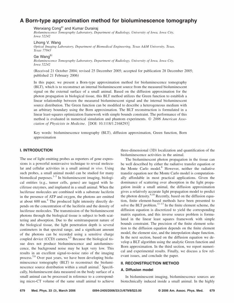
A Born-type approximation method for bioluminescence tomography Wenxiang Cong a and Kumar Durairaj Bioluminescence Tomography Laboratory, Department of Radiology, University of Iowa, Iowa City, Iowa 52242 Lihong V. Wang Optical Imaging Laboratory, Department of Biomedical Engineering, Texas A&M University, Texas, Texas 77843 Ge Wang b Bioluminescence Tomography Laboratory, Department of Radiology, University of Iowa, Iowa City, Iowa 52242 Received 21 October 2004; revised 25 December 2005; accepted for publication 28 December 2005; published 21 February 2006 In this paper, we present a Born-type approximation method for bioluminescence tomography BLT, which is to reconstruct an internal bioluminescent source from the measured bioluminescent signal on the external surface of a small animal. Based on the diffusion approximation for the photon propagation in biological tissue, this BLT method utilizes the Green function to establish a linear relationship between the measured bioluminescent signal and the internal bioluminescent source distribution. The Green function can be modified to describe a heterogeneous medium with an arbitrary boundary using the Born approximation. The BLT reconstruction is formulated in a linear least-squares optimization framework with simple bounds constraint. The performance of this method is evaluated in numerical simulation and phantom experiments. © 2006 American Asso- ciation of Physicists in Medicine. DOI: 10.1118/1.2168293 Key words: bioluminescence tomography BLT, diffusion approximation, Green function, Born approximation I. INTRODUCTION The use of light emitting probes as reporters of gene expres- sions is a powerful noninvasive technique to reveal molecu- lar and cellular activities in a small animal in vivo. Using such probes, a small animal model can be studied for many biomedical purposes. 1–3 In bioluminescent imaging, biologi- cal entities e.g., tumor cells, genes are tagged with lu- ciferase enzymes, and implanted in a small animal. When the luciferase molecules are combined with a substrate luciferin in the presence of ATP and oxygen, the photons are emitted at about 600 nm. 4 The produced light intensity directly de- pends on the concentration of the luciferin and the density of luciferase molecules. The transmission of the bioluminescent photons through the biological tissue is subject to both scat- tering and absorption. Due to the semitransparent nature of the biological tissue, the light penetration depth is several centimeters in that spectral range, and a significant amount of the photons can be recorded using a sensitive charge coupled device CCD camera. 4,5 Because the biological tis- sue does not produce bioluminescence and autolumines- cence, the background noise may be kept very low. This results in an excellent signal-to-noise ratio of the imaging process. 5,6 Over past years, we have been developing biolu- minescence tomography BLT to reconstruct the biolumi- nescence source distribution within a small animal. 7 Specifi- cally, bioluminescent data measured on the body surface of a small animal can be processed in reference to a correspond- ing micro-CT volume of the same small animal to achieve three-dimensional 3D localization and quantification of the bioluminescence activities in the animal. The bioluminescent photon propagation in the tissue can be well described by either the radiative transfer equation or the Monte Carlo model. 8 However, neither the radiative transfer equation nor the Monte Carlo model is computation- ally affordable in most practical applications. Given the dominance of scattering over absorption in the light propa- gation inside a small animal, the diffusion approximation gives a relatively accurate light propagation model to predict the photon density. 9,10 Recently, based on the diffusion equa- tion, finite element-based methods have been presented to solve the BLT problem. 11–13 In the finite element scheme, the diffusion equation is discretized to yield the corresponding matrix equation, and this inverse source problem is formu- lated in the linear least squares framework with simple bounds constraint. The precision of the finite element solu- tion to the diffusion equation depends on the finite element model, the element size, and the interpolation shape function. In the next section, based on the diffusion equation we de- velop a BLT algorithm using the analytic Green function and Born approximation. In the third section, we report numeri- cal and experimental results. Finally, we discuss a few rel- evant issues, and conclude the paper. II. RECONSTRUCTION METHOD A. Diffusion model In bioluminescent imaging, bioluminescence sources are biotechnically induced inside a small animal. In the highly 679 679 Med. Phys. 33 „3…, March 2006 0094-2405/2006/33„3…/679/8/$23.00 © 2006 Am. Assoc. Phys. Med.
-
Upload
periyarmaniammai -
Category
Documents
-
view
0 -
download
0
Transcript of A Born-type approximation method for bioluminescence tomography
A Born-type approximation method for bioluminescence tomographyWenxiang Conga� and Kumar DurairajBioluminescence Tomography Laboratory, Department of Radiology, University of Iowa, Iowa City,Iowa 52242
Lihong V. WangOptical Imaging Laboratory, Department of Biomedical Engineering, Texas A&M University, Texas,Texas 77843
Ge Wangb�
Bioluminescence Tomography Laboratory, Department of Radiology, University of Iowa, Iowa City,Iowa 52242
�Received 21 October 2004; revised 25 December 2005; accepted for publication 28 December 2005;published 21 February 2006�
In this paper, we present a Born-type approximation method for bioluminescence tomography�BLT�, which is to reconstruct an internal bioluminescent source from the measured bioluminescentsignal on the external surface of a small animal. Based on the diffusion approximation for thephoton propagation in biological tissue, this BLT method utilizes the Green function to establish alinear relationship between the measured bioluminescent signal and the internal bioluminescentsource distribution. The Green function can be modified to describe a heterogeneous medium withan arbitrary boundary using the Born approximation. The BLT reconstruction is formulated in alinear least-squares optimization framework with simple bounds constraint. The performance of thismethod is evaluated in numerical simulation and phantom experiments. © 2006 American Asso-ciation of Physicists in Medicine. �DOI: 10.1118/1.2168293�
Key words: bioluminescence tomography �BLT�, diffusion approximation, Green function, Born
approximationI. INTRODUCTION
The use of light emitting probes as reporters of gene expres-sions is a powerful noninvasive technique to reveal molecu-lar and cellular activities in a small animal in vivo. Usingsuch probes, a small animal model can be studied for manybiomedical purposes.1–3 In bioluminescent imaging, biologi-cal entities �e.g., tumor cells, genes� are tagged with lu-ciferase enzymes, and implanted in a small animal. When theluciferase molecules are combined with a substrate luciferinin the presence of ATP and oxygen, the photons are emittedat about 600 nm.4 The produced light intensity directly de-pends on the concentration of the luciferin and the density ofluciferase molecules. The transmission of the bioluminescentphotons through the biological tissue is subject to both scat-tering and absorption. Due to the semitransparent nature ofthe biological tissue, the light penetration depth is severalcentimeters in that spectral range, and a significant amountof the photons can be recorded using a sensitive chargecoupled device �CCD� camera.4,5 Because the biological tis-sue does not produce bioluminescence and autolumines-cence, the background noise may be kept very low. Thisresults in an excellent signal-to-noise ratio of the imagingprocess.5,6 Over past years, we have been developing biolu-minescence tomography �BLT� to reconstruct the biolumi-nescence source distribution within a small animal.7 Specifi-cally, bioluminescent data measured on the body surface of asmall animal can be processed in reference to a correspond-
ing micro-CT volume of the same small animal to achieve679 Med. Phys. 33 „3…, March 2006 0094-2405/2006/33„3
three-dimensional �3D� localization and quantification of thebioluminescence activities in the animal.
The bioluminescent photon propagation in the tissue canbe well described by either the radiative transfer equation orthe Monte Carlo model.8 However, neither the radiativetransfer equation nor the Monte Carlo model is computation-ally affordable in most practical applications. Given thedominance of scattering over absorption in the light propa-gation inside a small animal, the diffusion approximationgives a relatively accurate light propagation model to predictthe photon density.9,10 Recently, based on the diffusion equa-tion, finite element-based methods have been presented tosolve the BLT problem.11–13 In the finite element scheme, thediffusion equation is discretized to yield the correspondingmatrix equation, and this inverse source problem is formu-lated in the linear least squares framework with simplebounds constraint. The precision of the finite element solu-tion to the diffusion equation depends on the finite elementmodel, the element size, and the interpolation shape function.In the next section, based on the diffusion equation we de-velop a BLT algorithm using the analytic Green function andBorn approximation. In the third section, we report numeri-cal and experimental results. Finally, we discuss a few rel-evant issues, and conclude the paper.
II. RECONSTRUCTION METHOD
A. Diffusion model
In bioluminescent imaging, bioluminescence sources are
biotechnically induced inside a small animal. In the highly679…/679/8/$23.00 © 2006 Am. Assoc. Phys. Med.

680 Cong et al.: A Born-type approximation method for bioluminescence tomography 680
scattering biological tissue, the diffusion approximation togives a quite accurate description of the bioluminescent lightpropagation in the small animal,9,10,14
− � · �D�r� � ��r�� + �a�r���r� = S�r� �r � �� ,
�1�D�r� = �3��a�r� + �1 − g��s�r���−1,
where � denotes the region of interest for the object, ��r�the photon density �Watts/mm2�, S�r� the energy density dis-tribution of a light source �Watts/m3�, D�r� diffusion coef-ficient, �a�r� the absorption coefficient �mm−1�, �s�r� thescattering coefficient �mm−1�, and g the anisotropy param-eter. The optical parameters �a�r�, �s�r�, and g can be inde-pendently determined; for example, from the literature or thediffuse optical tomography technique. Assuming that the ex-periment is performed in an ideal dark environment, and nophoton comes in an inward direction at the boundary. Takinginto account the mismatch between the refractive indices nwith � and n� in the surrounding medium, the boundarycondition can be expressed as14,15
��r� + 2Cnd�r�D�r��� · ���r�� = 0 �r � ��� , �2�
where � is the unit outer normal on ��, Cnd�r�= �1+R�r�� / �1−R�r��. In the experiment, the medium surround-ing � is air, for which n� is approximately 1. Therefore, R�r�only depends on the refractive index n of the medium, andcan be approximated by R�−1.4399n−2+0.7099n−1
+0.6681+0.0636n. The measured quantity is the outgoingphoton density on ��,15
Q�r� = − D�r��� · ���r�� =1
2Cnd�r���r� �r � ��� . �3�
B. Reconstruction formula
Clearly, BLT is to reconstruct the 3D source distributionS�r� from the two-dimensional �2D� measured outgoing pho-ton density Q�r� on �� based on �1�–�3�. This is typicalunderdetermined and ill-posed problem, and much more dif-ficult than the associated forward problem. Wang et al. dis-cussed the solution uniqueness for the BLT problem undersome practical constraint conditions, and established that theunique solution or semiunique solution is possible by incor-porating sufficiently a priori knowledge, including the opti-cal parameters of the anatomy, the region and form of thelight source.16
According to the partial differential equation theory, thesolution to �1�–�3� can be expressed in terms of its Greenfunction G�rd ,rs�,
��rd� = ��s
S�rs�G�rd,rs�drs �rs � �s,rd � ��� , �4�
where S�rs� is the light source density at location rs, �s is asubregion ��s��� to be predetermined from a prioriknowledge, in which a bioluminescent source distributionmay present, and rd is the detector position. The Green func-
tion G�rd ,rs� can be numerically computed; for example,Medical Physics, Vol. 33, No. 3, March 2006
using finite differences, finite elements or Monte Carlomethod. While the direct computation is expensive, a Born-type approximation approach can be used to simplify theprocedure for the Green function G�rd ,rs�. In an infinite ho-mogeneous medium, the Green function has an analyticform:10
Gh�rd − rs� =exp�− �effrd − rs�
4�Drd − rs,
�5�
��Gh�� − r� = − �eff +1
� − r� � − r
� − rGh�� − r� ,
where �eff= ��a /D�1/2 is the effective attenuation coefficient.In order to obtain the Green function for arbitrary bound-aries, we can partition the body surface of a small animalinto N facets, each of which has an area �Sb and a surfacenormal nb. Using the Kirchhoff approximation �KA� and ex-trapolated boundary condition, the complete Green functionGb�rd ,rs� for a homogeneous medium and boundary condi-tion �2� can be expressed by the Green function Gh�rd ,rs�,
17
Gb�rd,rs� = Gh�rd,rs� − �b=1
N
W�rd,rb�Gh�rb − rd�
��Gh�r1� − Gh�r2���S�rb� ,
�6�
W�rd,rb� = 1
2CndD− �rd − rb�nb · �rd − rb�� ,
where r1= rs−rb, r2= 4CndD�CndD− �rs−rb� ·nb�+r12, and
function �r� is defined as �r�= ��eff+ �1/r���1/r�. Since areal animal body is not homogeneous, it should be consid-ered as heterogeneous medium. According to the perturba-tion theory,18 the optical parameters may be decomposed intobackground values �D0 and �a
0� and its perturbation value�D and �a�, that is D�r�=D0+D�r�, �a�r�=�a
0�a�r�.Hence, the Green function in the heterogeneous medium canbe expressed in an integral form19
G�rd,rs� = Gb�rd,rs� + ��
Gb�rd,����� · �D�����G��,rs��
− �a���G��,rs��d� . �7�
Therefore, the desired Green function G�rd ,rs� can be ob-tained by an iterative procedure based on �7�. In general, theBorn method produces a relatively accurate approximation tothe exact Green function G�rd ,rs� in the small perturbationcase, and G�rd ,rs� in the heterogeneous medium under theboundary condition �2� can be formulated as20
G�rd,rs� = Gb�rd,rs� − ��
Gb�rd,��Gb��,rs��a���d�
− ���
Gb�rd,��Gb��,rs�D���
2CndD���d�
− � ���Gb�rd,��� · ���Gb��,rs��D���d� . �8�
�
681 Cong et al.: A Born-type approximation method for bioluminescence tomography 681
The gradients ��G�rd ,�� and ��G�� ,rs� in �8� are obtainedaccording to the following formulas:
��Gb�rd,�� = ��Gh�rd,�� + �b=1
N
�W�rd,rb�Gh�rb − rd�
�P�r1,r2��S�rb�� ,
�9�P�r1,r2� = �Gh�r1��r1� − Gh�r2��r2���� − rp�
+ 2CndDGh�r2��r2�nb
and
��Gb��,rs� = ��Gh��,rs� − �b=1
N
H��,rb�Gh�rb − ��
��Gh�r1� − Gh�r2���S�rb� ,
�10�
H��,rb� =nb · �� − rb�
� − rb2��eff
2 + 3�� − rb���� − rb�
− �� − rb� �� − rb�2CndD
+ nb� .
Now, the linear relationship between the predicted photondensity on the domain boundary and the bioluminescencesource strength has been established as summarized by�4�–�10�. Since BLT is an ill-posed problem, an effectiveapproach is to find a regularized solution by minimizing thefollowing objective function:21
min0�S�rs��U�rs�
��Q�rd� − Qmeas�rd��W2 + � �S�� ,
�11�
Q�rd� =1
2Cnd�
�s
G�rd,rs�S�rs�drs,
where W is a weighting matrix and norm �V�W2 =VTWV,
U�rs� denotes an upper bound on S�rs� to be physicallymeaningful, �S� a stabilizing functional, � the regulariza-tion parameter to balance �S� and �Q�rd�−Qmeas�rd��W
2 .
III. EXPERIMENTAL RESULTS
A. Born approximation
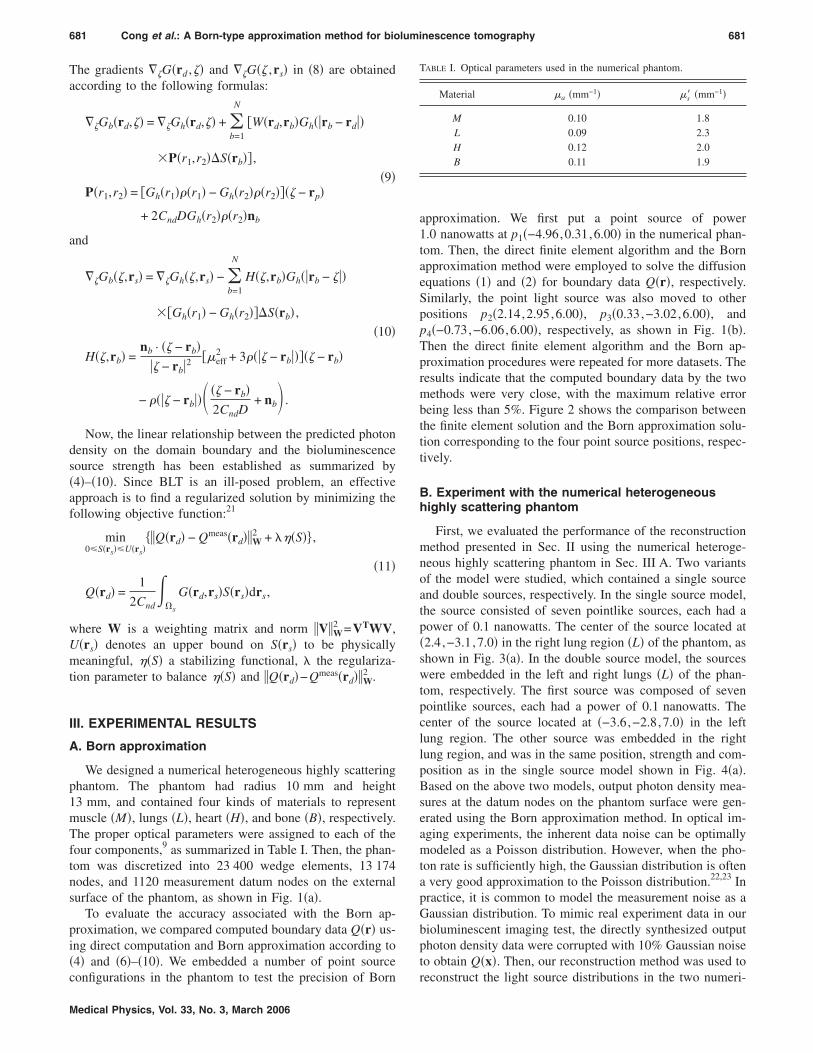
We designed a numerical heterogeneous highly scatteringphantom. The phantom had radius 10 mm and height13 mm, and contained four kinds of materials to representmuscle �M�, lungs �L�, heart �H�, and bone �B�, respectively.The proper optical parameters were assigned to each of thefour components,9 as summarized in Table I. Then, the phan-tom was discretized into 23 400 wedge elements, 13 174nodes, and 1120 measurement datum nodes on the externalsurface of the phantom, as shown in Fig. 1�a�.
To evaluate the accuracy associated with the Born ap-proximation, we compared computed boundary data Q�r� us-ing direct computation and Born approximation according to�4� and �6�–�10�. We embedded a number of point source
configurations in the phantom to test the precision of BornMedical Physics, Vol. 33, No. 3, March 2006
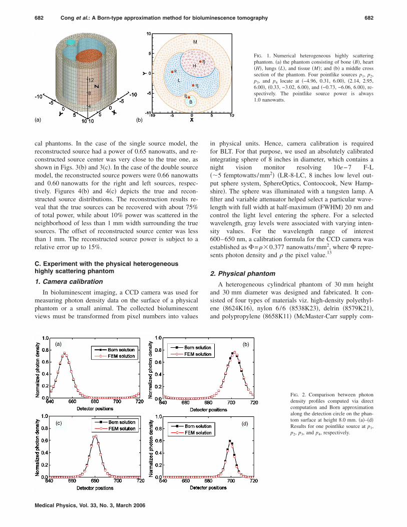
approximation. We first put a point source of power1.0 nanowatts at p1�−4.96,0.31,6.00� in the numerical phan-tom. Then, the direct finite element algorithm and the Bornapproximation method were employed to solve the diffusionequations �1� and �2� for boundary data Q�r�, respectively.Similarly, the point light source was also moved to otherpositions p2�2.14,2.95,6.00�, p3�0.33,−3.02,6.00�, andp4�−0.73,−6.06,6.00�, respectively, as shown in Fig. 1�b�.Then the direct finite element algorithm and the Born ap-proximation procedures were repeated for more datasets. Theresults indicate that the computed boundary data by the twomethods were very close, with the maximum relative errorbeing less than 5%. Figure 2 shows the comparison betweenthe finite element solution and the Born approximation solu-tion corresponding to the four point source positions, respec-tively.
B. Experiment with the numerical heterogeneoushighly scattering phantom
First, we evaluated the performance of the reconstructionmethod presented in Sec. II using the numerical heteroge-neous highly scattering phantom in Sec. III A. Two variantsof the model were studied, which contained a single sourceand double sources, respectively. In the single source model,the source consisted of seven pointlike sources, each had apower of 0.1 nanowatts. The center of the source located at�2.4,−3.1,7.0� in the right lung region �L� of the phantom, asshown in Fig. 3�a�. In the double source model, the sourceswere embedded in the left and right lungs �L� of the phan-tom, respectively. The first source was composed of sevenpointlike sources, each had a power of 0.1 nanowatts. Thecenter of the source located at �−3.6,−2.8,7.0� in the leftlung region. The other source was embedded in the rightlung region, and was in the same position, strength and com-position as in the single source model shown in Fig. 4�a�.Based on the above two models, output photon density mea-sures at the datum nodes on the phantom surface were gen-erated using the Born approximation method. In optical im-aging experiments, the inherent data noise can be optimallymodeled as a Poisson distribution. However, when the pho-ton rate is sufficiently high, the Gaussian distribution is oftena very good approximation to the Poisson distribution.22,23 Inpractice, it is common to model the measurement noise as aGaussian distribution. To mimic real experiment data in ourbioluminescent imaging test, the directly synthesized outputphoton density data were corrupted with 10% Gaussian noiseto obtain Q�x�. Then, our reconstruction method was used to
TABLE I. Optical parameters used in the numerical phantom.
Material �a �mm−1� �s� �mm−1�
M 0.10 1.8L 0.09 2.3H 0.12 2.0B 0.11 1.9
reconstruct the light source distributions in the two numeri-
682 Cong et al.: A Born-type approximation method for bioluminescence tomography 682
cal phantoms. In the case of the single source model, thereconstructed source had a power of 0.65 nanowatts, and re-constructed source center was very close to the true one, asshown in Figs. 3�b� and 3�c�. In the case of the double sourcemodel, the reconstructed source powers were 0.66 nanowattsand 0.60 nanowatts for the right and left sources, respec-tively. Figures 4�b� and 4�c� depicts the true and recon-structed source distributions. The reconstruction results re-veal that the true sources can be recovered with about 75%of total power, while about 10% power was scattered in theneighborhood of less than 1 mm width surrounding the truesources. The offset of reconstructed source center was lessthan 1 mm. The reconstructed source power is subject to arelative error up to 15%.
C. Experiment with the physical heterogeneoushighly scattering phantom
1. Camera calibration
In bioluminescent imaging, a CCD camera was used formeasuring photon density data on the surface of a physicalphantom or a small animal. The collected bioluminescentviews must be transformed from pixel numbers into values
Medical Physics, Vol. 33, No. 3, March 2006
in physical units. Hence, camera calibration is requiredfor BLT. For that purpose, we used an absolutely calibratedintegrating sphere of 8 inches in diameter, which contains anight vision monitor resolving 10e−7 F-L��5 femptowatts/mm2� �LR-8-LC, 8 inches low level out-put sphere system, SphereOptics, Contoocook, New Hamp-shire�. The sphere was illuminated with a tungsten lamp. Afilter and variable attenuator helped select a particular wave-length with full width at half-maximum �FWHM� 20 nm andcontrol the light level entering the sphere. For a selectedwavelength, gray levels were associated with varying inten-sity values. For the wavelength range of interest600–650 nm, a calibration formula for the CCD camera wasestablished as �=�0.377 nanowatts/mm2, where � repre-sents photon density and the pixel value.13
2. Physical phantom
A heterogeneous cylindrical phantom of 30 mm heightand 30 mm diameter was designed and fabricated. It con-sisted of four types of materials viz. high-density polyethyl-ene �8624K16�, nylon 6/6 �8538K23�, delrin �8579K21�,and polypropylene �8658K11� �McMaster-Carr supply com-
FIG. 1. Numerical heterogeneous highly scatteringphantom. �a� the phantom consisting of bone �B�, heart�H�, lungs �L�, and tissue �M�; and �b� a middle crosssection of the phantom. Four pointlike sources p1, p2,p3, and p4 locate at �−4.96, 0.31, 6.00�, �2.14, 2.95,6.00�, �0.33, −3.02, 6.00�, and �−0.73, −6.06, 6.00�, re-spectively. The pointlike source power is always1.0 nanowatts.
FIG. 2. Comparison between photondensity profiles computed via directcomputation and Born approximationalong the detection circle on the phan-tom surface at height 8.0 mm. �a�–�d�Results for one pointlike source at p1,p2, p3, and p4, respectively.

683 Cong et al.: A Born-type approximation method for bioluminescence tomography 683
pany, Chicago, IL�. The four regions M, L, H, and B in thephantom represent the polyethylene, nylon, delrin, and poly-propylene, respectively, as shown in Fig. 5�a�. The lumines-cent light sticks �Glowproducts, Victoria, British Columbia,Canada� were used as light sources. The stick consisted of aglass vial containing one chemical solution and a larger plas-tic vial containing another solution with the former beingembedded in the latter. By bending the plastic vial, the glassvial can be broken to mix the two solutions and emit redlight around 650 nm. Two small holes of diameter 0.6 mmand height 3 mm were drilled in the phantom with their cen-ters at �−9.0,1.5,15.0� and �−9.0,−1.5,15.0� in the left Lregion of the phantom. Two catheter tubes about 1.9 mmheight were filled with red luminescent liquid, and wereplaced inside the two holes as light sources, respectively.
Medical Physics, Vol. 33, No. 3, March 2006
Emitting light power of two catheter tubes was measuredwith the CCD camera. They are 105.1 nanowatts and97.4 nanowatts, respectively.
3. Optical parameters
Since the optical parameters were needed for BLT, we hadto determine them for the four components �M, H, L, and B�of the physical phantom. Four homogeneous cylindricalphantoms with diameter 20 mm and height 20 mm weremade of the above-mentioned four kinds of materials, re-spectively. The light about 650 nm was output from the exitport of the integrating sphere, and guided into a small holewith 10 mm depth of one specimen through the optic fiber.In a dark environment, the specimen was imaged and cap-
FIG. 3. BLT reconstruction of onesource in the right L region of a mousemodel. �a� A middle cross-section ofthe phantom with the true source dis-tribution of power 0.70 nanowatts, �b�2D graphics of the reconstructedsource distribution, and �c� 3D graph-ics of the reconstructed source distri-bution from the surface data corruptedby 10% Gaussian noise, and truesource and reconstructed source distri-bution are displayed using low inten-sity and high intensity, respectively.
FIG. 4. BLT reconstruction of twosources in the left and right L region,respectively. �a� A middle cross-section of the phantom with the truesource distribution, �b� 2D graphics ofthe reconstructed source distribution,and �c� 3D graphics of the recon-structed source distribution from thesurface data corrupted by 10% Gauss-ian noise, and true source and recon-structed source distribution are dis-played using low intensity and highintensity lines, respectively.

684 Cong et al.: A Born-type approximation method for bioluminescence tomography 684
tured the output photon on the other surface of the specimenusing cooled CCD camera �Roper Scientific Inc, Trenton,NJ� with an exposure time of 30 seconds. Then, the surfaceoutput photon density was calculated by transforming thepixel values in the CCD image into the light unit accordingto our experimentally established calibration formula. Thespecimen was modeled as a semi-infinite homogeneous me-dium. The steady-state diffusion theory was applied with theextrapolated boundary condition that the photon density waszero at an artificial boundary parallel to the boundary of themedium. Then, an analytic formula was used to predict thephoton density on the bottom surface. Finally, a nonlinearleast square fitting was done to determine the absorption co-efficient �a and the reduced scatter coefficient �s�. The cal-culated optical parameters of the four regions are given inTable II.13
4. Data acquisition
The heterogeneous phantom containing the two lightsources was placed on the sample holder in front of the CCDcamera. Then, the data acquisition was performed in a darkenvironment along four horizontal orientations 90 degreesapart. During each acquisition, one luminescent view wastaken by exposing the camera for 60 seconds, as shown inFig. 6. A permissible source region �s was assigned by ana-lyzing the four luminescent views taken by the CCD camera.These four planar images exhibited high value clusters nearthe center of the front image and a low value distribution inthe back image. On the right-hand side and left-hand sideimages, it was seen that one side displayed high values while
TABLE II. Optical parameters estimated for the heterogeneous highly scat-tering phantom.
Material �a �mm−1� �s� �mm−1�
T 0.0068 1.031L 0.0233 2.000H 0.0104 1.096B 0.0001 0.060
Medical Physics, Vol. 33, No. 3, March 2006
the other side showed low values. From these observations,we infer that the light source region should be in the frontpart of the phantom. Along the longitudinal direction, highvalues were clustered around z=15 mm relative to the phan-tom bottom. Consequently, the permissible source regionwas specified as
�s = ��x,y,z�− 12.0 � x � − 6.0,− 7.0 � y � 7.0,13.0
� z � 17.0� .
5. BLT reconstruction
To simulate the photon propagation in the phantom, ageometrical model of diameter 30 mm and height 20.66 mmwas established corresponding to a middle section of thephysical phantom. Based on this geometrical model, a finite-element discrete model was built consisting of 13 608 wedgeelements and 7809 nodes with 1216 datum nodes on thephantom surface, as shown in Fig. 7�a�. The optical proper-ties of every element were assigned in reference to the opti-
FIG. 5. Physical heterogeneous highly scattering phan-tom. �a� A photography of the highly scattering phan-tom consisting of polyethylene �M�, nylon �L�, delrin�H�, and polypropylene �B�; and �b� a middle cross sec-tion through two small hollow cylinders for hostingsources in the L region.
FIG. 6. Luminescent views on the cylindrical phantom surface taken using aCCD camera in four horizontal directions 90 degrees apart. �a� Front, �b�
back, �c� left-hand side, and �d� right-hand side views of the phantom.
685 Cong et al.: A Born-type approximation method for bioluminescence tomography 685
cal parameters reported in Sec. III C 3. On the surface of thegeometric model 19 circles were selected, separated by1.148 mm, along each of which 64 detection locations wereuniformly distributed. The pixel values of the luminescentviews were transformed into corresponding physical units.The measured photon density at each detector location wasobtained from the luminescent images �Fig. 6�. The com-puted photon density at the corresponding detection pointwas obtained using �3� and �4� in Sec. II. Then, the recon-struction method described in Sec. II was applied to recon-struct the light source distribution in the heterogeneous phan-tom. The reconstructed results correctly revealed that therewere two light sources in the phantom, their center located at�−8.24,2.75,15.0� and �−8.24,−2.79,15.0� with total power76.3 nanowatts and 67.6 nanowatts, respectively. Each lightsource just consisted of up-and-down two point-like sourcesseparated about 2 mm, matching the real cylinder lightsource inside phantom. The pointlike source at a node can beregarded as an equivalent spherical source with a corre-sponding power and radius estimated as half an average sizeof the element edges. Figure 7 shows both a photograph ofthe phantom and the reconstructed source distribution. Thedifferences between the reconstructed and real source posi-tions were less than 1.5 mm. The relative errors in the sourcepower were 27% and 31% for the two sources, respectively.The computed surface photon density profiles based on thereconstructed light sources were in good agreement with theexperimental counterparts, with the average relative error be-ing 11%. Two representative photon density profiles for the
Medical Physics, Vol. 33, No. 3, March 2006
comparison between the computed and measured photondensity on the side surface of the phantom were shown inFig. 8.
IV. DISCUSSION AND CONCLUSIONS
The above-described results have demonstrated the feasi-bility of our reconstruction method for BLT. In the numericalphantom experiment, even though the measured data on theexternal surface of the phantom were corrupted by 10%Gaussian noise, the light sources can be located fairly accu-rately, and source power can be recovered up to 85%. All thesimulation experiments we performed have shown that thealgorithm is fairly robust with respect to data noise and theinitial distribution in the optimization procedure. Our physi-cal phantom experiment has confirmed that the method canreliably identify light sources in the heterogeneous back-ground. The error of the reconstructed source location isabout 1.5 mm. The error of the reconstructed source power isabout 30%. Compared with the data we obtained in the nu-merical simulation, the reconstruction results for the physicalphantom may be further improved by using the radiativetransport equation instead of the diffusion equation, decreas-ing the element size, reducing the measurement noise, and soon. Although the total power of each reconstructed sourcewas close to the true power, the volumes of the reconstructedsources are different from the actual values, depending onthe mesh size. Generally, the smaller the mesh size we use,the higher accuracy we will achieve in reconstructing the
FIG. 7. BLT reconstruction of the twosources in the left L region from ex-perimental data. �a� A 3D rendering ofthe reconstructed sources �sphere� andreal sources �cylinder�; and �b� a 2Dgraphics of the reconstructed sources.
FIG. 8. Comparison between mea-sured and computational photon den-sity profiles along the detection circleon the phantom surface at heights �a�10.37 mm and �b� 17.27 mm.

686 Cong et al.: A Born-type approximation method for bioluminescence tomography 686
shape and/or size of the underlying source. A procedure forprogressive mesh refinement will help enhance the recon-struction quality, and will be explored in our future study.
In this work, we have established a direct linear relationbetween the light source distribution and the measured pho-ton density on the side surface of the object. The advantageover the finite element reconstruction method13 is that ourmethod does not involve an inverse matrix, and can handlemore complicated numerical models. Particularly, ourmethod is more suitable for parallel computing. In addition,this method will be more efficient in the case of smoothvarying optical properties consistent to Born approximationtheory.
Currently, we are working to perform living mouse stud-ies using the proposed reconstruction method. It would becritically important for BLT to be applied in biomedical ap-plications. Such in vivo BLT is highly challenging, involvinggeometrical modeling of the mouse, determination of opticalparameters, bioluminescent data acquisition, multiresolutioniterative reconstruction, and generation for a finite elementmesh of a heterogeneous, irregular and complicated object.
In conclusion, we have developed a Born-type approxi-mation method for BLT, obtained encouraging preliminaryresults in both numerical simulation and physical phantomexperiments, and established that our proposed method iseffective for BLT. In vivo mouse studies using our BLTmethod will be reported in the future.
ACKNOWLEDGMENT
This work is supported by NIH/NIBIB Grant No.EB001685.
a�Electronic mail: [email protected]�Electronic mail: [email protected]. Rudin and R. Weissleder, “Molecular imaging in drug discovery anddevelopment,” Nat. Rev. Drug Discovery 2, 123–131 �2003�.
2S. Wang, J. Petravicz, and X. O. Breakefield, “Bioluminescence Imagingof regulated gene expression using HSV-1 Amplicon vectors in rodentbrain,” Molecular Therapy 9, S27 �2004�.
3P. Ray, A. M. Wu, and S. S. Gambhir, “Optical bioluminescenceand positron emission tomography imaging of novel fusion reportergene in tumor xenografts of living mice,” Cancer Res. 63, 1160–1165�2003�.
4
C. H. Contag and M. H. Bachmann, “Advances in vivo bioluminescenceMedical Physics, Vol. 33, No. 3, March 2006
imaging of gene expression,” Annu. Rev. Biomed. Eng. 4, 235–260�2002�.
5B. W. Rice, M. D. Cable, and M. B. Nelson, “In vivo imaging of light-emitting probes,” J. Biomed. Opt. 6, 432–440 �2001�.
6T. C. Doyle, S. M. Burns, and C. H. Contag, “In vivo bioluminescenceimaging for integrated studies of infection,” Cell. Microbiol. 6, 303–317�2004�.
7G. Wang, E. A. Hoffman, G. McLennan, L. V. Wang, M. Suter, and J.Meinel, “Development of the first bioluminescent CT scanner,” Radiol-ogy 229(P), 566 �2003�.
8L.-H. Wang, S. L. Jacques, and L.-Q Zheng, “MCML—Monte Carlomodeling of light transport in multi-layered tissues,” Comput. MethodsPrograms Biomed. 47, 131–146 �1995�.
9A. J. Welch and M. J. C. van Gemert, Optical and Thermal Response ofLaser-Irradiated Tissue �Plenum, New York, 1995�.
10S. R. Arridge, “Optical tomography in medical imaging,” Inverse Probl.15, R41–R93 �1999�.
11W. Cong, D. Kumar, Y. Liu, A. Cong, and G. Wang, “A practical methodto determine the light source distribution in bioluminescent imaging,”Proc. SPIE 5535, 679–686 �2004�.
12X. Gu, Q. Zhang, L. Larcom, and H. Jiang, “Three-dimensional biolumi-nescence tomography with model-based reconstruction,” Opt. Express12, 3996–4000 �2004�.
13W. Cong, G. Wang, D. Kumar, Y. Liu, M. Jiang, L. V. Wang, E. A.Hoffman, G. McLennan, P. B. McCray, J. Zabner, and A. Cong, “Practi-cal reconstruction method for bioluminescence tomography,” Opt. Ex-press 13, 6756–6771 �2005�.
14J. J. Duderstadt and L. J. Hamilton, Nuclear Reactor Analysis �Wiley,New York, 1976�.
15M. Schweiger, S. R. Arridge, M. Hiraoka, and D. T. Delpy, “The finiteelement method for the propagation of light in scattering media: Bound-ary and source conditions,” Med. Phys. 22, 1779–1792 �1995�.
16G. Wang, Y. Li, and M. Jiang, “Uniqueness theorems in bioluminescencetomography,” Med. Phys. 31, 2289–2299 �2004�.
17J. Ripoll, M. Nieto-Vesperinas, R. Weissleder, and V. Ntziachristos, “Fastanalytical approximation for arbitrary geometries in diffuse optical to-mography,” Opt. Lett. 27, 527–529 �2002�.
18S. Economou, Green’s Functions in Quantum Physics �Springer-Verlag,New York, 1983�.
19V. A. Markel, and J. C. Schotland, “Inverse problems in optical diffusiontomography. I. Fourier-Laplace inversion formulas,” J. Opt. Soc. Am. A18, 1336–1347 �2001�.
20M. A. O’Leary, Dissertation, University of Pennsylvania, 1996.21P. P. B. Eggermont, “Maximum entropy regularization for fredholm inte-
gral equation of the first kind,” SIAM J. Math. Anal. 24, 1557–1576�1993�.
22J. C. Ye et al., “Optical diffusion tomography by iterative coordinate—Descent optimization in a Bayesian framework,” J. Opt. Soc. Am. A 16,2400–2412 �1999�.
23E. Waks, K. Inoue, W. D. Oliver, E. Diamanti, and Y. Yamamoto, “High-efficiency photon-number detection for quantum information processing,”
IEEE J. Sel. Top. Quantum Electron. 9, 1502–1511 �2003�.