4D seismic imaging of a CO2 plume 1

4D seismic imaging of an injected CO2 plume at the Sleipner Field, central North Sea R.A. Chadwick1, R. Arts2, O. Eiken3, G.A. Kirby1, E. Lindeberg4 & P. Zweigel4

1British Geological Survey, Kingsley Dunham Centre, Keyworth, Nottingham, United Kingdom, NG12 5GG. E-mail: rach@bgs.ac.uk. 2Netherlands Institute of Applied Geoscience TNO - National Geological Survey, Kriekenpitplein 18, PO Box 80015, 3508 TA Utrecht, The Netherlands 3Statoil Research Centre, Rotvoll, N-7005 Trondheim, Norway 4Sintef Petroleum Research, N-7465 Trondheim, Norway Corresponding author: R.A. Chadwick Words of text: 5570 (including abstract, references figure captions) References: 8 Tables: 0 Figures: 15 Abstract: CO2 produced at the Sleipner field is being injected into the Utsira Sand, a major saline aquifer. Time-lapse seismic data acquired in 1999, with 2.35 million tonnes of CO2 in the reservoir, image the CO2 plume as a number of bright sub-horizontal reflections. These are interpreted as tuned responses from thin (< 8 m thick) layers of CO2 trapped beneath intra-reservoir shales. A prominent vertical ‘chimney’ of CO2 appears to be the principal feeder of these layers in the upper part of the reservoir. Amplitude – thickness scaling for each layer, followed by a layer summation, indicates that roughly 80% of the total injected CO2 is concentrated in the layers. The remainder is interpreted to occupy the feeder ‘chimneys’ and dispersed clouds between the layers. A prominent velocity pushdown is evident beneath the CO2 accumulations. Velocity estimation using the Gassmann relationships suggests that the observed pushdown cannot readily be explained by CO2 present only at high saturations in the thin layers; a minor proportion of low saturation CO2 is also required. This is consistent with the layer volume summation, but significant uncertainty remains. [end of abstract] CO2 separated from natural gas produced at the Sleipner field in the central North Sea (Norwegian block 15/9) is currently being injected into the Utsira Sand, a major saline aquifer some 26000 km2 in area (Fig. 1). Injection started in 1996 and is planned to continue for about twenty years, at a rate of about one million tonnes per year. The Saline Aquifer CO2 Storage (SACS) project aims to monitor the injected CO2 by time-lapse seismic methods. Baseline 3D seismic data were acquired in 1994, prior to injection. A first repeat survey, covering some 26 km2, was acquired in October 1999, with 2.35 million tonnes of CO2 in the reservoir, and a second repeat survey was acquired in September 2001 with 4.26 million tonnes of CO2 in situ.

4D seismic imaging of a CO2 plume 2

Current findings from the 1994 and 1999 surveys are described here, with vivid 4D seismic images of the CO2 plume being used to illustrate the ongoing interpretive and modelling work.

Background to the injection operation

The Utsira Sand forms part of the Mio-Pliocene Utsira Formation (Gregersen et al. 1997, Chadwick et al. 2001). It is axially-situated within the thick post-rift succession of the central North Sea, forming a basin-restricted lowstand deposit of considerable extent, over 400 km from north to south and typically 50 – 100 km west to east. Sleipner lies towards the southern limit of the Utsira Sand (Fig. 1a), where the reservoir is some 800 to 1000 m deep and between 200 and 300 m thick. Core measurements, petrographic analysis and well logs (Zweigel et al. 2001) show the sand to be clean and largely uncemented with porosities in the range 0.30 to 0.42, typically 0.37. Well logs from the Sleipner area however resolve thin beds of intra-reservoir mudstone or shale, characterised by high γ-ray readings (Fig. 2). The shales range in thickness from less than a metre to more than five metres, but with a well-defined modal peak at just over one metre (Zweigel et al. 2001). The Utsira Sand is overlain by the Nordland Formation (Isaksen & Tonstad 1989), which mostly comprises prograding deltaic wedges of Pliocene age. These generally coarsen upwards, from mudstones in the deeper, axial parts of the basin to silt and sand in the shallower and more marginal parts. In the Sleipner area the lowest unit, a 50-100 m thick silty mudstone, forms the immediate reservoir caprock. CO2 was injected into the Utsira reservoir at a depth of 1012 m below sea level (bsl), beneath a gentle domal closure of some 12 m relief (Fig. 3a). The CO2 occupies an enveloping 3D volume which is here termed the ‘CO2 plume’. The plume lies between the injection point and the top of the reservoir at about 800 m bsl, where estimated formation temperatures, based on a downhole measurement, are 36ºC and 29ºC respectively. At these conditions the CO2 is in the form of a supercritical fluid with a roughly constant density of around 700 kgm-3, (the tendency for density to decrease with increasing temperature is counterbalanced by the increasing pressure, Span & Wagner, 1996). The mass of 2.35 MT injected by October 1999 would correspond therefore to a volume of about 3.3 x 106 m3 at reservoir conditions. Uncertainty in reservoir temperature and the effect of minor impurities such as methane, permit the possibility of lower densities, perhaps down to about 600 kgm-3, with a corresponding in situ CO2 volume of 3.8 x 106 m3. Irrespective of the precise reservoir conditions, the principal driving force for the migration of CO2 up through the reservoir is buoyancy, due the density difference, , between CO2 and brine.

Reflectivity of the CO2 plume

Introducing CO2 into the Utsira reservoir has a dramatic effect on reflectivity. The 1994 pre-injection data (Fig. 3a), show moderate reflections from the top and base of the reservoir, with much weaker intra-reservoir events (the mid-Utsira reflection is a seabed multiple of the prominent events near to the top of the reservoir). In contrast, the 1999 data show a clear image of the CO2 plume with strong reflections at a number of levels within the reservoir (Fig. 3b). These are interpreted as layers of CO2 accumulating or ‘ponding’ beneath the thin intra-reservoir shales. The CO2 related reflections do not show the gentle antiformal geometry of the Utsira stratigraphy as

4D seismic imaging of a CO2 plume 3

imaged on the 1994 data, but rather show a downward pointing V-profile, which becomes more pronounced down through the reservoir. This is interpreted as an effect of velocity pushdown within the plume. A time-slice through the plume on difference data (1999 minus 1994) shows it to be markedly elliptical in plan, elongated NNE-SSW, with a major axis of about 1800 m and a minor axis of some 600 m (Fig. 3c). The difference data also show complex structure within the plume, including vertical linear zones of amplitude reduction and relatively isolated volumes of CO2 (Fig. 3d). Reflections on the difference data beneath the injection point are interpreted as artefacts. These have two main causes: multiple energy (principally the seabed multiple) from the overlying plume, and ‘difference’ signal generated by the effects of velocity pushdown rather than by changes in reflectivity. Up to twelve individual reflection horizons can be identified in the plume (Fig. 4). These were picked on wavelet troughs, signifying negative acoustic impedance contrasts, which correspond approximately to the top of each CO2 layer (see below). The probable presence of multiple energy and the likelihood that the plume reflections represent composite interference wavelets makes it difficult to produce an unequivocal horizon interpretation and other, more conservative interpretations with somewhat fewer horizons cannot be discounted. Some of the interpreted horizons are large features, comparable in plan area to that of the whole plume, others form much smaller outliers. The two small uppermost horizons are interpreted to lie right at the top of the Utsira Sand, directly beneath the caprock (Fig. 4).

Thin bed effects

The twelve picked horizons have a total plan area of about 2.9 x 106 m2. Taking an injected CO2 volume of 3.3 x 106 m3, and a mean reservoir porosity of 0.37, if the CO2 were wholly distributed as reflective sub-horizontal layers, these layers would, on average, be only about 3 m thick. Because CO2 is also interpreted to be present as chimneys between the layers (see below), the actual average layer thickness would be less than 3 m. With layer thicknesses generally beneath the limit of seismic resolution (λ/4, ~8 m for these data), the observed CO2 reflectivity is likely to be largely a consequence of thin-layer interference. With thin-layers, reflection amplitude is related directly to layer thickness, increasing from zero at zero layer thickness, to a maximum at the tuning thickness (Fig. 5). Thus, observed amplitudes on the picked horizons, which tend to increase systematically inwards, from zero at their outer edges to a maximum value near their centres (e.g. Fig. 6a), are consistent with a tuned response from thin layers of CO2 which thicken from zero at their outer edge to a maximum in the axial part of the plume, within the structural closure. The highest amplitudes moreover, are encountered in the central parts of the most areally extensive horizons. Dominantly thin-layer reflectivity is also consistent with the observed seismic waveforms, which comprise mostly interference doublets, rather than the near-symmetrical, near-zero phase processed input wavelet (this is well displayed at simple acoustic interfaces such as the seabed). Assuming that the maximum amplitudes observed in the plume correspond to the tuning thickness of about 8m (in practice they may correspond to a somewhat lesser thickness), and making a simplifying linear interpolation, amplitude can be scaled directly to layer thickness for each horizon. For example, in the layer corresponding to Horizon X, maximum amplitudes are comparable with the highest amplitudes observed in the plume, so its maximum calculated thickness approaches 8 m (Fig. 6b).

4D seismic imaging of a CO2 plume 4

CO2 chimneys

Intriguing detail is visible in parts of the plume (Fig. 7). Beneath the gentle closure at the top of the Utsira Sand, the main reflections show the characteristic V-profile velocity pushdown, which builds rapidly downwards. In the southern part of the plume, a vertical column of reduced horizon reflectivity corresponds precisely to a more localised pushdown, itself superimposed on the broader V-profile. The amount of this localised pushdown increases rapidly downwards from the reservoir top to reach a maximum of about 20 ms at about 970 ms two-way time. It does not clearly change beneath this, but tends to smear somewhat, becoming rather diffuse at base Utsira level. The feature is interpreted as a vertical ‘chimney’ of moderate or high CO2 saturation, in the upper part of the plume. This causes a rapid buildup of pushdown within the chimney itself and a pushdown shadow below. Similar, though much less prominent seismic features seen elsewhere in the plume are interpreted as smaller CO2 chimneys. The relationship of the main CO2 chimney to the surrounding reflective layers is exemplified by Horizon Y (Fig. 7). The horizon dips in two-way time towards the chimney, due to the velocity pushdown in the axial parts of the plume. Horizon Y is the most extensive individual reflection within the plume and in plan view shows marked lateral amplitude variations (Fig. 8a). The chimney is visible as a ‘hole’ in the amplitude map where the horizon autotracker has not been able to pick the event (Fig. 7). It is surrounded by high amplitude reflections, particularly to the east, where a ‘stream’ of enhanced reflectivity is prominent in the east and north. A perspective view of the horizon (Fig. 8b), with reflection amplitudes draped over its two-way time topography, shows the prominent pushdown depression around the chimney, with linear ridgelike features to the north. The ridge crests correspond to markedly enhanced seismic amplitudes that are interpreted as due to small changes in thickness of the CO2 layer. Thus CO2 migrating laterally away from the chimney, beneath a thin shale, forms thicker ‘ponds’ beneath local topographic culminations. These give rise to higher reflection amplitudes as the CO2 layer approaches the tuning thickness (Fig. 9). Their ridgelike morphologies may be put down to primary sedimentary, channel-related structures within the Utsira Sand, or, perhaps more likely, to differential compaction within what remain largely unconsolidated strata (Zweigel et al. 2001). Whatever their underlying cause, it is likely that the amplitude variations are effectively mapping thickness changes in the CO2 layer down to less than one metre, which more-or-less corresponds to the noise threshold. It is notable that the main CO2 chimney is situated nearly, though not perfectly, above the injection point (Fig. 7), close to the outer limit of the 95% confidence ellipse of the well position. It is tempting to suppose that the chimney location is linked directly to that of the injection point, however, because of the positional uncertainty, some form of pre-existing geological control cannot be ruled out.

Verification aspects

The 4D data provide two essentially independent means of quantitatively assessing the amount of CO2 in the subsurface.

4D seismic imaging of a CO2 plume 5

Thin layer summation

The capillary pressure, pc, between the formation brine and the injected CO2 will cause the CO2 saturation, SCO2, to vary with height, h, in each CO2 layer. The gradient can be computed by balancing the buoyancy, · g · h, with the capillary pressure. In SI units: ·g ·h = pc = 810.35(1- SCO2)

-0.948 Equation 1 The capillary pressure - saturation relationship was determined by centrifuge experiments on core material from the Utsira Sand (SACS unpublished data). The variation of SCO2 with h was thereby computed and also the average value of SCO2 for a range of layer thicknesses (Fig. 10). Using this information the layer thicknesses derived for each reflecting horizon (e.g. Fig. 6b) can be converted to net CO2 thickness (e.g. Fig. 6c). This was carried out at each grid point (CMP), by multiplying the layer thickness by the average CO2 saturation (Fig. 10), and by the reservoir porosity. Summation of these net thicknesses for each layer gives a first order estimate of the total amount of CO2 imaged by the seismic data. For the interpretation presented here (Fig. 4), the total volume in thin layers is estimated at about 2.6 x 106 m3; about 80% of the known injected volume. A number of factors, alone or in combination, will contribute to uncertainty in this figure. These include uncertainty in the horizon interpretation (including interference between adjacent tuning wavelets), errors in the simple amplitude to thickness conversion, the presence of dispersed (essentially unreflective) CO2 in between the reflective layers, dissolution of CO2 into the formation water and amplitude loss in the deeper plume due to signal attenuation.

Velocity Pushdown

The velocity pushdown of reflections beneath the CO2 plume (Fig. 11) provides an alternative means of estimating CO2 volume in situ. By interpreting the base Utsira Sand beneath the plume on both the 1994 and 1999 surveys it is possible to map the pushdown beneath much of the CO2 plume (Fig. 11c). Significant uncertainty arises however because reflections on the 1999 data are locally degraded and the mapping shows some instability beneath the outer parts of the plume where pushdown values are small. An alternative approach is to map the pushdown automatically by cross-correlating a window of the sub-plume reflections on the 1994 and 1999 surveys, and thereby deriving a pushdown time-lag for each seismic trace (Fig 11d). Pushdown values derived in this way are more stable than the interpreted map beneath the outer parts of the bubble, but high pushdown values directly beneath the main CO2 chimney are not resolved, due to degradation of the cross-correlogram by poor signal to noise ratios. Irrespective of the method of derivation, the pushdown anomaly is elliptical in plan, with time-lags in excess of 20 ms widely observed beneath the central parts of the plume and locally in excess of 40 ms. The total amount of pushdown caused by the plume can be expressed as the individual time-lags at each CMP trace (or bin), summed over the entire anomaly. This is termed the Total Area Integrated Time Delay (TAITD). The pushdown mapped by interpretation of the Base Utsira Sand (Fig. 11c), has a TAITD of about 11000 m2s, whereas the pushdown from cross-correlation (Fig. 11d) has a TAITD value of about 9200 m2s. Optimal mapping of the pushdown would probably incorporate both cross-correlation and local manual picking with a likely intermediate value of TAITD.

4D seismic imaging of a CO2 plume 6

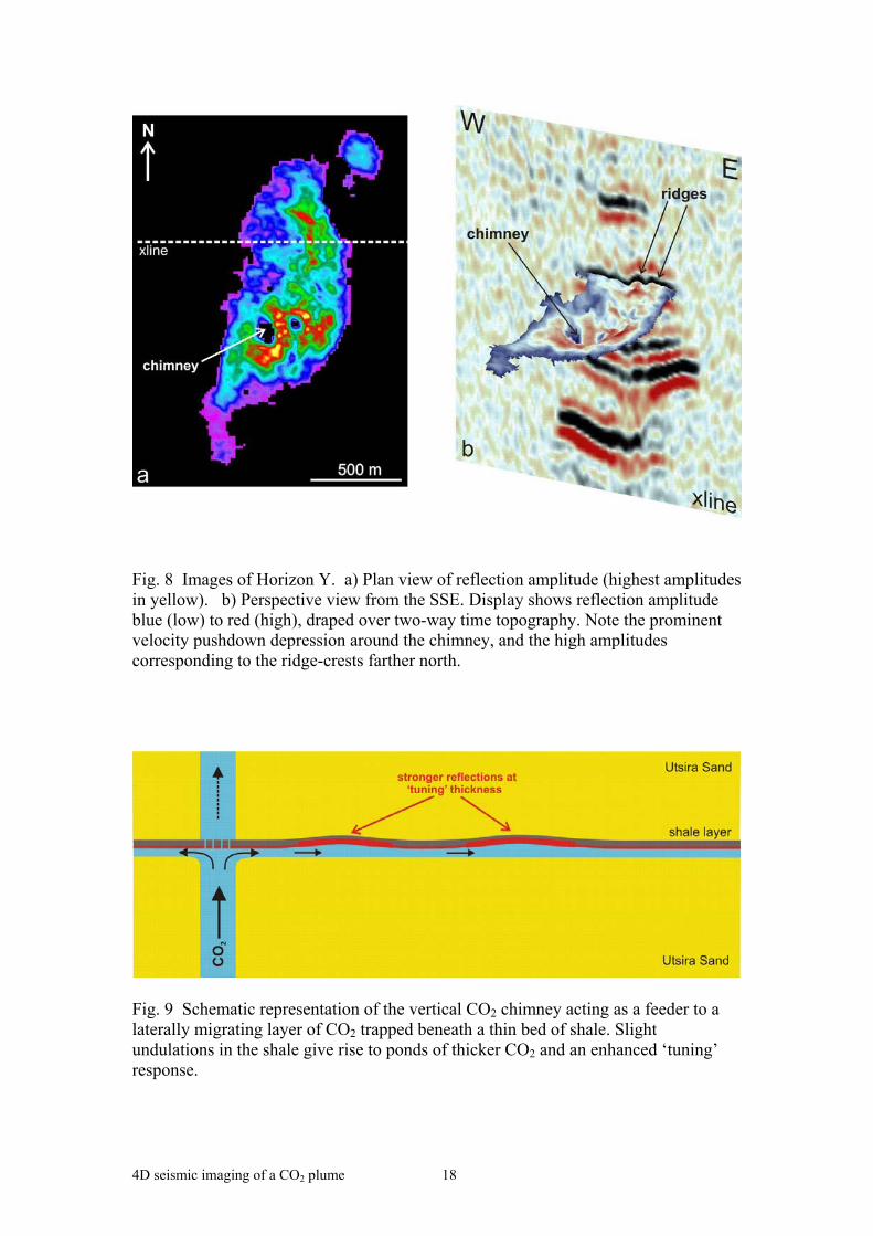
The amount of pushdown can be related algebraically to the column of CO2 in the overlying strata (Fig. 12). For each grid point (CMP):

2

22

SCOSW

SCOSW

VV

δyδxZVVδyδxΔT

Equation 2

where: ΔT is the time delay at each trace (T99survey – T94 survey) δx = x-dimension of bin (12.5 m for the SACS data) δy = y-dimension of bin (12.5 m for the SACS data) Vsw = seismic velocity of water-saturated rock VSCO2 = seismic velocity of rock saturated with CO2 (at saturation SCO2) Z = thickness of rock saturated with CO2 (at saturation SCO2) Substituting reservoir porosity () and CO2 saturation (SCO2) and summing all the grid points over the whole pushdown anomaly:

22

222

COSCOSW

SCOSW

SVV

e of COcted volumTotal injeVVδyδxΔT

Equation 3

In principal therefore, the TAITD, ΣΔT·δx·δy, can be related directly to the total volume of CO2 in the plume. In practice however there are significant uncertainties, particularly with respect to the expression below, here termed the ‘Pushdown Factor’:

22

22

COSCOSW

SCOSW

SVV

VV

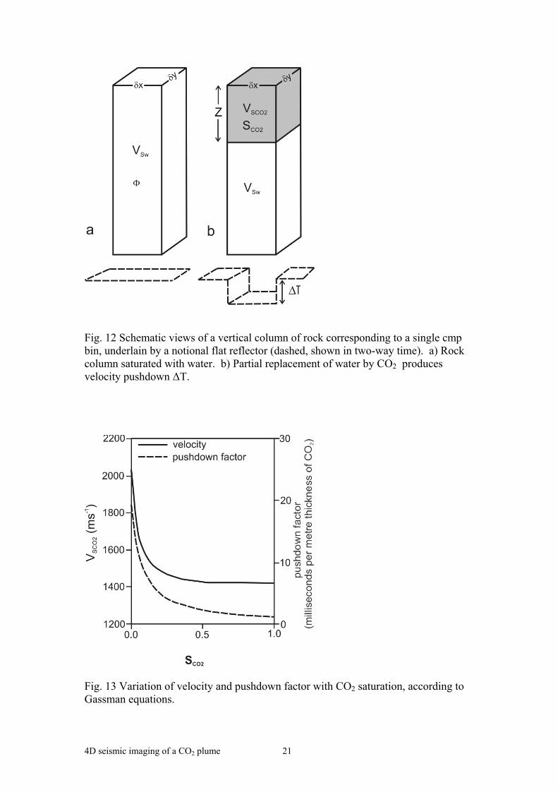
The Pushdown Factor has units of sm-1 and expresses the amount of pushdown in seconds (or, more conveniently, milliseconds), per net metre thickness of CO2. To calculate the Pushdown Factor, seismic velocities in rock filled with CO2 at various saturations can be estimated using the Gassmann fluid substitution equations (Gassmann 1951). Velocities derived in this way show a decrease from the observed value of about 2050 ms-1 in water-saturated sand, to about 1420 ms-1 in wholly CO2 saturated sand (Fig. 13). Errors are related mostly to uncertainties in elastic parameters, principally the bulk moduli of the rock framework and of supercritical CO2. In addition, the Gassmann equations assume a homogeneous mix of fluids, and a more patchy distribution would give a more linear behaviour of the velocity-saturation relationship. Pressure effects on the seismic velocities are expected to be negligible. No significant increase in pressure has been observed during the injection process so far, the CO2 flowing easily into the very high permeability reservoir. The pressure-temperature conditions of the reservoir around the CO2 plume are such that the CO2 is expected to remain in a supercritical state.

4D seismic imaging of a CO2 plume 7

Direct observation of velocity pushdown within the plume lends support to the Gassmann analysis. Around and within the CO2 chimney in the upper part of the plume (Fig. 7), a total pushdown of 22 ms develops over an estimated 60 m section of reservoir sand. This requires a seismic velocity of about 1450 ms-1 within the chimney, broadly consistent with Gassmann-derived values for CO2 saturations in the range 0.3 to 1.0 (Fig. 13). This is in accord with both the moderate saturations for vertical conduits proposed by Johnson et al. (2001) and the higher saturations indicated by Lindeberg et al. (2001). Overall, sensitivity analysis suggests that velocity error does not comprise the main source of uncertainty in calculating the Pushdown Factor (see below). Most of the velocity decrease induced by CO2 takes place at low saturations, the velocity curve levelling out at values of SCO2 greater than about 0.3 (Fig. 13). This ambiguity, together with the fact that SCO2 is an explicit term in the Pushdown Factor, renders the value of SCO2 the main source of uncertainty in the pushdown calculation. Thus the Pushdown Factor varies from over 25 milliseconds per net metre of CO2 at very low saturations of CO2, to only 1 – 2 milliseconds per net metre of CO2 at high saturations. CO2 at low saturations is therefore a much more efficient pushdown agent than higher saturation CO2. This leads to inherent uncertainty; to calculate the pushdown from a known injected volume, it is necessary also to know the effective saturation of CO2 throughout the plume. Forward modelling can be used to address the problem. TAITDs have been calculated for a series of assumed plume saturation scenarios based on the total volume of the plume envelope (Fig. 14). The two saturation ‘end-members’ will be considered first. The minimum saturation case is represented by CO2 distributed homogeneously throughout the entire volume of the plume envelope (Fig. 14a). The CO2 has a uniformly low saturation (SCO2 = 0.075) and generates a TAITD of 30802 m2s. This represents the theoretical maximum possible pushdown for the injected volume of CO2 and the observed plume geometry. The opposite end-member is the maximum saturation case, where CO2 is present only in a state of full saturation (SCO2 = 1.0), such as in discrete fully saturated layers (Fig. 14b). The TAITD in this case is only 3801 m2s, which represents the minimum theoretical pushdown for the known injected volume of CO2. Neither of the end-member scenarios matches the observed TAITD values. The low saturation end-member generates a pushdown that is much too high, and moreover, is not realistic in terms of the observed plume reflectivity. The full saturation end-member produces a pushdown that is much too low. Because the observed TAITD does lie between the end-member saturation limits, it can, therefore, be modelled by some intermediate saturation distribution. Bearing in mind the observed reflectivity, a reasonable saturation scenario is one where CO2 in the plume is partitioned into two separate components: a ‘reflective’ component of CO2 trapped in thin layers, each obeying the thickness-saturation function (Fig. 10), and an ‘unreflective’ component of diffuse, low saturation CO2, which occupies all or part of the volume in between the layers. Models based on this scenario took the component of CO2 in layers as the volume calculated by thin layer summation (see above). From this, the time-lag was calculated (Equation 2), using the layer thickness-saturation function, at each CMP, for each horizon (e.g. Fig. 6d). The TAITD for the component of CO2 in layers was

4D seismic imaging of a CO2 plume 8

then obtained by summing over the 12 horizons, giving a value of 3784 m2s (Fig. 14c). This is much lower than the observed TAITDs, but the model is incomplete, in that it contains only about 80% of the total injected amount of CO2. Additional pushdown will result from the remaining 20% of CO2, which is assumed to form a diffuse, low-saturation component, in between the layers. The simplest two-component model (Fig. 14d) assumes that the remaining diffuse CO2 is homogeneously distributed throughout the intra-layer volume. The additional pushdown due to this diffuse CO2 is 9913 m2s, amply demonstrating the very high pushdown efficiency of low saturation CO2. The resultant TAITD of 13697 m2s is however considerably higher than the observed range of 9200 - 11000 m2s. A refinement of the model can be effected by the intuitively reasonable step of preferentially concentrating the diffuse CO2 in the central, axial parts of the plume. A simple concentric saturation distribution, increasing linearly from SCO2 = 0.0 at the plume edge, to SCO2 ~ 0.06 at the plume centre (Fig. 14e) has the same total injected volume but with a TAITD of 12847 m2s, significantly closer to the observed range. Further increasing the heterogeneity of the diffuse CO2 component, by concentrating it into localised volumes of higher saturation, has the effect of further decreasing the overall pushdown. Thus, the likely presence of chimneys of CO2 would effect an additional reduction in the calculated pushdown, probably to within the observed range. Alternatively, an observed pushdown lower than the calculated value may simply signify that rather more CO2 is trapped in the thin layers, at high saturations, than is indicated by the simple amplitude-thickness transformation. The effects of dissolution should not be discounted either, because dissolved CO2 would effectively become seismically invisible, rendering observed pushdowns smaller than predicted. Johnson et al. (2001) indicate however that in the first three years of injection, even with lateral dispersal of CO2 by trapping beneath shales, amounts of CO2 dissolving in the formation waters are likely to be small (<5%).

Pushdown - Amplitude relationships

In the above, reflection amplitudes and velocity pushdown give estimates of in situ CO2 volume that are essentially independent. It is also fruitful to examine these two seismic parameters together, as their inter-relationships provide additional useful insights. Velocity pushdown increases strongly towards the centre of the plume with a pronounced area of elevated values (~40ms or greater) around and east of the injection point (Fig.15a). Total plume amplitudes show a different pattern however (Fig. 15b), particularly across the central part of the plume where they are more evenly distributed, without notably increased values east of the injection point. This different behaviour can be quantified as variation in the pushdown – amplitude ratio (Fig.15c). The pushdown - amplitude ratio is analogous to the Pushdown Factor in that it measures pushdown per unit total reflection amplitude (the latter being related to total CO2 layer thickness). The observed variation of pushdown – amplitude ratio (Fig.15c) can therefore be interpreted as providing qualitative insights into saturation distribution. The outer parts of the plume, particularly in the NE and SW, farthest from the injection point, are characterised by low pushdown – amplitude ratios. These

4D seismic imaging of a CO2 plume 9

are interpreted as areas where CO2 is present only at high saturations in thin, reflective layers, which produce relatively small amounts of pushdown (cf Fig. 12). In contrast, the inner parts of the plume show much higher ratios. These are interpreted as signifying the presence of diffuse, low saturation CO2 between the layers, which produces additional pushdown but no additional reflectivity. A further effect, which would tend to reinforce the observed pattern, is a possible reduction in layer reflectivity where diffuse CO2 decreases the acoustic contrast of the high saturation layers. This is exemplified by the main CO2 chimney, which with its high pushdown, but subdued reflectivity (Figs. 6, 15b), is marked by a prominent localised area of high pushdown – amplitude ratio (Fig. 15c). The interplay of different seismic effects is quite complex, but the underlying pattern is clear; elevated pushdowns in the central part of the plume do not correspond to similarly enhanced reflectivity, and thereby indicate the presence of diffuse, unreflective CO2. This very much supports the preferred saturation model of Fig.14e and suggests that analysis of the relationships between velocity pushdown and plume reflectivity is a potentially powerful tool for mapping saturation distributions within the plume.

Conclusions and discussion

The time-lapse seismic data clearly image CO2 within the reservoir, both as sub-horizontal high amplitude reflections and also as a pronounced velocity pushdown. It is likely that much of the CO2 is present as thin layers, trapped beneath thin beds of low permeability shale. Though the CO2 layers themselves are mostly beneath the limit of seismic resolution, amplitude changes appear able to resolve thickness changes down to one metre or less. The data also resolve a prominent vertical feature, interpreted as a chimney of CO2. Reflection amplitudes and the build-up of velocity pushdown around the chimney indicate that the higher CO2 layers in the plume tend to thicken towards it, consistent with it forming the primary feeder of CO2 in the upper part of the plume. A number of similar though much less prominent features seen elsewhere in the plume may correspond to smaller chimneys. This is supported by some reservoir flow simulations (e.g. Lindeberg et al. 2000), which require a number of chimneys to feed the observed CO2 layers. The verticality of the main chimney may also offer intriguing insights into the way that CO2 migrates through the reservoir. Given that the probability of fortuitous vertical alignment of stratigraphical holes in the shale layers is rather small, the chimney seems to require that the column of CO2 is able to find its way rather easily through the thin shale beds. How this occurs is unclear. Sample data are limited, but intrinsic permeability seems unlikely, the buoyancy pressure of the CO2 column being probably too small to overcome the capillary entrance pressure (Lindeberg 1996). The 1994 data show little clear evidence of pre-injection faulting within the upper part of the reservoir, but small faults, close to the limit of seismic resolution, with displacements sufficient to provide pathways through the thin shale beds may be present, perhaps as a consequence of differential compaction. Another possibility is that the CO2 dehydrates the shales and thereby induces shrinkage cracks. Alternatively, in these weak, unconsolidated sediments, it may be that the buoyancy force of the CO2 column in the chimney is able to displace the thin shale layers by purely mechanical means. More circumstantial evidence for minor faulting in the

4D seismic imaging of a CO2 plume 10

reservoir is the likelihood of diffuse CO2 in between the main layers, which suggests that the thin shale horizons possess some degree of permeability. An important aspect of the time-lapse seismic imaging is its ability to quantify the amount of injected CO2 and any changes that subsequently occur due to leakage or dissolution. The studies carried out so far suggest that the observed reflectivity and velocity pushdown are broadly consistent with the known injected volume of CO2. However considerable uncertainty remains in a number of areas, in particular, the likely presence of low saturation ‘diffuse’ CO2 in between the more concentrated layers. Because this diffuse CO2 is both unreflective and makes a disproportionately large contribution to the total pushdown, it introduces a strong element of non-uniqueness to the saturation models. The presence of low saturation CO2 within the plume is consistent with reservoir flow models carried out in the SACS project using the SIMED simulator (van der Meer et al. 2000) and with the reaction-transport models of Johnson et al. (2001), which incorporate semi-permeable (microfractured) intra-reservoir shales. Work is continuing on the time-lapse datasets and, with acquisition of the second repeat survey in September 2001, it is anticipated that understanding of the CO2 migration and dispersal will improve still further. We thank the SACS consortium for permission to publish this work. Permission to publish is also given by the Executive Director, British Geological Survey (NERC). SACS is funded by the EU Thermie Programme, by industry partners Statoil, BP, Exxon, Norsk Hydro, TotalFinaElf and Vattenfall, and by national governments. R&D partners are BGS (British Geological Survey), BRGM (Bureau de Recherches Geologiques et Minieres), GEUS (Geological Survey of Denmark), IFP (Institute Francais du Petrole), TNO-NITG (Netherlands Institute of Applied Geoscience – National Geological Survey) and SINTEF Petroleum Research.

4D seismic imaging of a CO2 plume 11

References Chadwick, R.A., Holloway, S., Kirby, G.A., Gregersen, U. & Johannessen, P.N. 2001. The Utsira Sand, Central North Sea – an assessment of its potential for regional CO2

disposal. In: Williams, D.J., Durie, R.A., McMullan, P., Paulson, C.A.J. & Smith, A.Y. (eds): Greenhouse Gas Control Technologies. CSIRO Publishing, Collingwood, Australia, 349 – 354. Gassmann, F., 1951. Über die Elastizität poröser Medien. Vierteljahresschr. der Naturf. Gesellschaft in Zürich, 96, 1-23. Gregersen, U., Michelsen, O. & Sorensen, J.C. 1997. Stratigraphy and facies distribution of the Utsira Formation and the Pliocene sequences in the northern North Sea. Marine and Petroleum Geology, 14, 893-914. Isaksen, D. & Tonstad, K. 1989. A revised Cretaceous and Tertiary lithostratigraphic nomenclature for the Norwegian North Sea, Norwegian Petroleum Directory, Bulletin 5. Johnson, J.W., Nitao, J.J., Steefel, C.I., and Knauss, K.G., 2001, Reactive transport modeling of geologic CO2 sequestration in saline aquifers: the influence of intra-aquifer shales and the relative effectiveness of structural, solubility, and mineral trapping during prograde and retrograde sequestration: Proceedings of the First National Conference on Carbon Sequestration, Washington, DC, May 14-17, 2001, 60 p., UCRL-JC-146932. Lindeberg, E.G.B. 1996. Escape of CO2 from Aquifers. Energy Conversion Management, Volume 38 Supplement, s229 – s234. Lindeberg, E., Zweigel, P., Bergmo, P., Ghaderi, A. & Lothe, A. 2001. Prediction of CO2 distribution pattern by geology and reservoir simulation and verified by time lapse seismic. In: Williams, D.J., Durie, R.A., McMullan, P., Paulson, C.A.J. & Smith, A.Y. (eds): Greenhouse Gas Control Technologies. CSIRO Publishing, Collingwood, Australia, 372 – 377. Span, R. & Wagner, W. 1996. A New Equation of State for Carbon Dioxide covering the Fluid Region from the Triple-Point to 1100 K at Pressures up to 800 MPa. Journal of Physical and Chemical Reference Data, 25/6. van der Meer, L.G.H., Arts, R.J., Peterson, L., 2000. Prediction of migration of CO2 injected into a saline aquifer: Reservoir history matching to a 4D seismic image with a compositional Gas/Water model. In: Williams, D.J., Durie, R.A., McMullan, P., Paulson, C.A.J. & Smith, A.Y. (eds): Greenhouse Gas Control Technologies, CSIRO Publishing, Collingwood, Australia, 378-384.

Zweigel, P., Arts, R., Bidstrup, T., Chadwick, A., Eiken, O., Gregersen, U., Hamborg, M., Johanessen, P., Kirby, G., Kristensen, L., & Lindeberg, E., 2001. Results and experiences from the first Industrial-scale underground CO2 sequestration case (Sleipner Field, North Sea). American Association of Petroleum Geologists, Annual Meeting, June 2001, Denver, abstract volume (CD) 6p.

4D seismic imaging of a CO2 plume 12

Figures

Fig. 1 a) Limits and thickness of the Utsira Sand and location of the Sleipner injection point. b) Cartoon of the Sleipner CO2 injection operation.

Fig. 2 Geophysical logs (γ-ray and sonic) in wells close to Sleipner. The Utsira Sand has much lower γ-ray (gr) signature than the caprock succession. γ-ray peaks within the sand (main peaks arrowed) are interpreted as thin beds of shale. Note the injection well is strongly deviated and the drilled sequence will differ from that at the plume location.

4D seismic imaging of a CO2 plume 13

Fig. 3 Time-lapse seismic images of the CO2 plume a) Crossline through the 1994 dataset prior to injection - IP denotes injection point. b) Crossline as in (a) through the 1999 dataset, showing enhanced reflectivity and velocity pushdown. c) Time-slice at 950 ms (~870 m) through the difference dataset (1999-1994). Blue denotes a negative acoustic impedance contrast. d) Oblique line through the difference dataset (1999-1994) showing complex plume structure (arrow denotes position of time-slice). Enhanced amplitude display with red/yellow denoting a negative acoustic impedance contrast.

4D seismic imaging of a CO2 plume 14

Fig. 4 3-D view of the picked horizons within the 1999 plume superimposed on part of an inline. Horizons X and Y labelled.

4D seismic imaging of a CO2 plume 15

Fig. 5 a) Acoustic impedance model with a thin shale overlying a layer of CO2 – saturated sand whose thickness increases from left to right. b) Seismic response of the above model. Green pick marks seismic trough corresponding to the top of the CO2 - saturated layer. In the Sleipner plume most reflectivity is a tuning response from CO2 – saturated layers less than 8 m thick, where amplitude is controlled by layer thickness.

4D seismic imaging of a CO2 plume 16

Fig. 6 Plan views of Horizon X. a) reflection amplitude b) thickness of rock - CO2 layer c) net thickness of CO2, assuming Ф = 0.37 and saturation-thickness function d) velocity pushdown (ms) due to layer.

4D seismic imaging of a CO2 plume 17

Fig. 7 Inline through the 1999 dataset. Note velocity pushdown at base of reservoir and also more localised pushdown interpreted as caused by a ‘chimney’ of CO2 in the upper part of the plume. Also note lateral amplitude variations on the individual reflections (e.g. Horizon Y with autopick). Blue denotes a negative acoustic impedance contrast. IP = approximate location of injection point (corrected for pushdown).

4D seismic imaging of a CO2 plume 18

Fig. 8 Images of Horizon Y. a) Plan view of reflection amplitude (highest amplitudes in yellow). b) Perspective view from the SSE. Display shows reflection amplitude blue (low) to red (high), draped over two-way time topography. Note the prominent velocity pushdown depression around the chimney, and the high amplitudes corresponding to the ridge-crests farther north.

Fig. 9 Schematic representation of the vertical CO2 chimney acting as a feeder to a laterally migrating layer of CO2 trapped beneath a thin bed of shale. Slight undulations in the shale give rise to ponds of thicker CO2 and an enhanced ‘tuning’ response.

4D seismic imaging of a CO2 plume 19

Fig. 10 Variation of average CO2 saturation with layer thickness.

4D seismic imaging of a CO2 plume 20

Fig. 11 Velocity pushdown beneath the CO2 plume. a) 1994 inline showing base Utsira Sand pick. b) 1999 inline showing base Utsira Sand pick (1994 pick for reference). Note higher pushdown beneath chimney. c) Map of two-way time pushdown based on manual interpretation of Base Utsira Sand (note high pushdown values SE of the injection point, beneath the main chimney) d) Map of pushdown based on cross-correlation of a window of events beneath the plume (note lack of high pushdowns associated with the chimney). IP denotes injection point. Black outline denotes outer edge of the plume reflectivity envelope.

4D seismic imaging of a CO2 plume 21

Fig. 12 Schematic views of a vertical column of rock corresponding to a single cmp bin, underlain by a notional flat reflector (dashed, shown in two-way time). a) Rock column saturated with water. b) Partial replacement of water by CO2 produces velocity pushdown ΔT.

Fig. 13 Variation of velocity and pushdown factor with CO2 saturation, according to Gassman equations.

4D seismic imaging of a CO2 plume 22

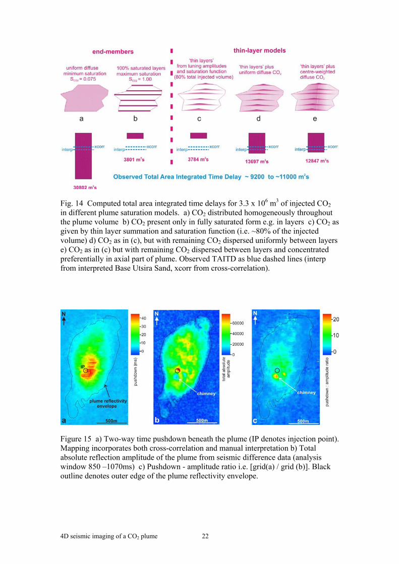
Fig. 14 Computed total area integrated time delays for 3.3 x 106 m3 of injected CO2 in different plume saturation models. a) CO2 distributed homogeneously throughout the plume volume b) CO2 present only in fully saturated form e.g. in layers c) CO2 as given by thin layer summation and saturation function (i.e. ~80% of the injected volume) d) CO2 as in (c), but with remaining CO2 dispersed uniformly between layers e) CO2 as in (c) but with remaining CO2 dispersed between layers and concentrated preferentially in axial part of plume. Observed TAITD as blue dashed lines (interp from interpreted Base Utsira Sand, xcorr from cross-correlation).

Figure 15 a) Two-way time pushdown beneath the plume (IP denotes injection point). Mapping incorporates both cross-correlation and manual interpretation b) Total absolute reflection amplitude of the plume from seismic difference data (analysis window 850 –1070ms) c) Pushdown - amplitude ratio i.e. [grid(a) / grid (b)]. Black outline denotes outer edge of the plume reflectivity envelope.