Segmentation of 4D Echocardiography Using Stochastic Online Dictionary Learning
Upload
khangminh22Category
view
0download
0

LARSA 4D Sample and Verification Problems
A manual for
LARSA 4DFinite Element Analysis and Design Software
Last Revised August 26, 2021
Copyright (C) 2001-2021 LARSA, Inc. All rights reserved. Information in thisdocument is subject to change without notice and does not represent a commitmenton the part of LARSA, Inc. The software described in this document is furnishedunder a license or nondisclosure agreement. No part of the documentation may bereproduced or transmitted in any form or by any means, electronic or mechanicalincluding photocopying, recording, or information storage or retrieval systems, forany purpose without the express written permission of LARSA, Inc.

LARSA 4D Sample and Verification Problems
Table of ContentsSamples for Linear Elastic Static Analysis 11
L01: 2D Truss with Static Loads 15Solution Comparison 15
L02: Beam with Elastic Supports 17Solution Comparison 18
L03: Beam on Elastic Foundation 19Solution Comparison 21Theoretical Results 22
L04: Space Truss Static Analysis 25Solution Comparison 26
L05: 2D Truss with Thermal Load 27Solution Comparison 27
L06: Static Analysis of a Space Frame 29Solution Comparison 31
L07: Plate Thermal Analysis 33Solution Comparison 34
L08: Shell-Bending of a Tapered Cantilever 35Solution Comparison 36
L10: Tie Beam without Geometric Stiffening 37Solution Comparison 38
L11: Circular Plate with a Hole Static Analysis 39Solution Comparison 40References 40
L12: Hemispherical Shell Static Analysis 41Solution Comparison 43References 43
L13: Cylindrical Roof Static Analysis 45Reference 46Solution Comparison 46
L14: 2D Truss - Thermal Loads and Settlement 49Solution Comparison 50
L16: Nonlinear Thermal Load 51Solution Comparison 51
L17: Plane Stress Element-Straight Beam with Static Loads 53Problem Description 53Loading 53Solution Comparison 54Conclusion 59
L18: Shell-Straight Beam with Static Loads 61Problem Description 61
3

LARSA 4D Sample and Verification Problems
Results 63References 69
L19: Shell-Twisted Beam with Static Loads 71Problem Description 71Loading 71Solution Comparison 72References 72
L20: Shell-Cylinder with Internal Pressure 73Problem Description 73Solution Comparison 74References 74
L21: Shell-Patch Test with Prescribed Displacements 77Problem Description 77Loading 77Solution Comparison 78References 80
L22: Shell-Patch Test Using Thermal Loading 81Problem Description 81Results 82References 84
L23: Shell-Plate on Elastic Foundation 85Problem Description 85Solution Comparison 85References 86
L24: Shell-Curved Beam with Static Loads 87Problem Description 87Loading 88Solution Comparison 88References 90
L25: Shell-Rectangular Plate with Static Loads 91Problem Description 91Solution Comparison 92References 94
L26: Shell-Scordelis-Lo Roof with Static Loads 97Problem Description 97Loading 97Solution Comparison 97
L27: Thermal Stresses in a Plate 107Problem Description 107Solution Comparison 107References 108
L28: Shell-Temperature Gradient Through Shell Thickness 109Problem Description 109Results 110
4

LARSA 4D Sample and Verification Problems
References 111L29: Solid-Straight Beam with Static Loads 113
Problem Description 113Data 113Loading 114Solution Comparison 125
L30: Solid-Twisted Beam with Static Loads 127Problem Description 127Loading 127Solution Comparison 128
L31: Non-Prismatic Beam with Nonlinear Thermal Load 129Problem Description 129Solution Comparison 131
L32: Isotropic Plate Cantilever using an Orthotropic MaterialDefinition
135
Problem Description 135Solution Comparison 140
L33: Cantilever with Orthotropic Material 143Problem Description 143Solution Comparison 147
L35: Plate Initial Strain Load 149Problem Description 149Solution Comparison 150
Samples for Nonlinear Elastic Static Analysis 153N01: Tie Beam with Geometric Stiffening 155
Solution Comparison 156Reference 156
N02: Cable with Hanging Loads 157Solution Comparison 157
N03: Beam on an Elastic Soil Foundation 159Solution Comparison 159Reference 160
N04: Truss with Misaligned Supports - Nonlinear Static 161Solution Comparison 161
N05: Nonlinear Analysis of Cable Roof 163Solution Comparison 163
N06: Diamond Shaped Frame - Geometric Nonlinear 165Reference 166Solution Comparison 166
N07: Diamond Shaped Frame - Geometric Nonlinear -Incremental Joint Displacement Loading
167
Reference 168Solution Comparison 168
5
LARSA 4D Sample and Verification Problems
N08: A High Arch Structure - Geometric Nonlinear 169Solution Comparison 170Reference 170
N09: Thermal Expansion to Close a Gap 171Solution Comparison 171
N13: Straight Cantilever Girder with Nonlinear Shell Elementsin Membrane Action
173
Problem Description 173Solution Comparison 174References 175
N14: Straight Cantilever Girder with Nonlinear Shell Elementsin Plate Action
177
Problem Description 177Solution Comparison 178References 179
N15: Slit Annular Plate with Vertical Load 181Problem Description 181Solution Comparison 182References 183
Samples for Eigenvalue Analysis 185E01: Triangular Cantilever Plate Eigenvalues 187
Solution Comparison 189Reference 189
E02: Square Cantilever Plate Eigenvalues 191Solution Comparison 193
E03: Beam Eigenvalues 195Solution Comparison 195
E04: Cantilever Beam Eigenvalues 197Solution Comparison 197
E05: Rectangular Cantilever Plate Eigenvalues 199Solution Comparison 201
E06: Mass Spring Model Eigenvalues 203Solution Comparison 205
E07: 2D Frame (Wilson & Bathe) Eigenvalues 207Solution Comparison 208References 208
E08: ASME Frame Eigenvalues 209Solution Comparison 210References 211
E09: Natural Frequencies of a Torsional System 213Solution Comparison 213
Samples for Stressed Eigenvalue Analysis 2156

LARSA 4D Sample and Verification Problems
ES01: Vibrations of Axially Loaded Beam - Nonlinear 217Solution Comparison 218
Samples for Response Spectra Analysis 219RSA01: 2D Frame with Static and Seismic Loads 221
Solution Comparison 224References 227
Samples for Time History Analysis 229TH01: Spring Mass System Time History Analysis 231
Solution Comparison 232TH02: Beam with Concentrated Mass & Dynamic Load 233
Solution Comparison 234TH03: Cantilever Beam Time History Analysis 237
Solution Comparison 239References 240
TH04: Dynamic Analysis of a Bridge 241Solution Comparison 241
TH05: Two dimensional frame with linear viscous damper 243Background 243Example Problem 243Solution and Comparison 245Nonlinear Dashpots 246Limitations 248References 248
TH15: Rolling Stock Analysis 249Model Setup 249Rolling Stock Analysis 252Moving Load Analysis 254Comparison of Results 255Dynamic Effect 257
Samples for Staged Construction Analysis 261S01: Creep Effects - Simple Span Concrete Beam 263S02: Creep and Shrinkage - Cantilevers Loaded at DifferentTimes
265
S03: Creep and Shrinkage - Use CEB-FIP model code 1990 inS02
267
S04: Creep and Shrinkage - Connect Aging Cantilevers 269S05: Creep and Shrinkage - Use CEB-FIP model code 1990 insample S04
271
S06: 3-Span Post-Tension Deck 273S07: Composite I-Girder with Time-Dependent Effects 279
Cross-Section Definition 2797

LARSA 4D Sample and Verification Problems
Model Geometry 279Construction Sequence 279Verification of Cross-Section Properties 280Verification of Self-Weight Loading 280Verification of the Time Effect on Elastic Modulus 282Verification of Shrinkage 283
S08: Time-Dependent Material Properties Effects 285Problem Definition 285Modeling 286Construction Sequence 289Verification of Creep 289Verification of Shrinkage 293
S08b: Time-Dependent Material Properties Effects 299Problem Definition 299Modeling 300Construction Sequence 305Verification of Creep 305Verification of Shrinkage 307
S09: Plates with Time-Dependent Material Effects 311Problem Definition 311Modeling 312Verification of Creep 314Verification of Shrinkage 314Verification of Elastic Modulus Change 315
S09b: Plates with Time-Dependent Material Effects(Orthotropic Material)
317
Problem Definition 317Modeling 318Verification of Creep 319Verification of Shrinkage 320Verification of Elastic Modulus Change 320
Samples for Influence-Based Analysis 321INF01: AASHTO LFD Simple Span 323
Model Setup 323Result Case Setup 324Accessing Results 325Solution Comparison 327
INF02: AASHTO LFD Three Span 329Model Setup 329Span Break Markers 331Result Case Setup 332Accessing Results 334
INF10: Influence Surface 337Model Setup 337
8

LARSA 4D Sample and Verification Problems
Result Case Setup 337Accessing Results 337
Samples for Steel Bridge Design and Rating 339SBD06: Straight Steel Plate Girder Bridge with 90 Degree Skew(LFD)
341
Problem Details 341Dead Load 344Live Load 344Model Generation 346Compound Element Result Extraction 350Non-Composite and Composite Dead Load Analysis Results 3512) Influence Surface Based Live Load Analysis 356
SBD07: Curved Steel Plate Girder Bridge With 60 Degree Skew(LFD)
369
Problem Details 369Dead Load 372Live Load 372Model Generation 374Compound Element Result Extraction 378Non-Composite and Composite Dead Load Analysis Results 3792) Influence Surface Based Live Load Analysis 385
SBD08: Three-Span Continuous Horizontally Curved CompositeSteel Tub-Girder Bridge
397
Problem Details 397Dead Load 404Live Load 404Load Combinations 404Modeling and Code Check in LARSA 4D - Steel Bridge Module (SBM) 405References 450
Samples for Composite Construction 451C01: Single Span with Roller under Vertical Load 453
Cross-Section Definition 453Model 455Cross-Sectional Properties 456Self-Weight Loading 457
C02: Staged Construction Analysis 461Composite Sequence States 461Self-Weight Loading 462Standard Staged Construction Analysis 463
C03: Time-Dependent Material Properties 469Cross-Section Definition 469Model 469Cross-Sectional Properties 470
9

LARSA 4D Sample and Verification Problems
Self-Weight Loading 471Time Effect on Elastic Modulus 472Shrinkage 474Creep 477References 477
C04: Thermal Loads 479Cross-Section Definition 479Model 481Analysis of Thermal Loads 481Uniform Thermal Load 482Linear Gradient Thermal Load 483Nonlinear Gradient Thermal Load 485
Samples for Buckling Analysis 489B01: Torsional Buckling of Crucifix Section with Shell Elements 491
Problem Description 491Solution Comparison 492References 492
B02: Lateral Buckling of I Section with Shell Elements 493Problem Description 493Solution Comparison 494References 494
B03: Lateral Torsional Buckling of C Section with ShellElements
495
Problem Description 495Solution Comparison 496References 496
10

LARSA 4D Sample and Verification Problems
Samples for Linear ElasticStatic Analysis
These samples provide an overview of the linear elastic static analysis.
For More Information, please refer to the following documentation.
• For help on linear static analysis, see Linear Static Analysis in LARSA 4D Reference Manual.
L01: 2D Truss with Static Loads 15Solution Comparison 15
L02: Beam with Elastic Supports 17Solution Comparison 18
L03: Beam on Elastic Foundation 19Solution Comparison 21Theoretical Results 22
L04: Space Truss Static Analysis 25Solution Comparison 26
L05: 2D Truss with Thermal Load 27Solution Comparison 27
L06: Static Analysis of a Space Frame 29Solution Comparison 31
L07: Plate Thermal Analysis 33Solution Comparison 34
L08: Shell-Bending of a Tapered Cantilever 35Solution Comparison 36
L10: Tie Beam without Geometric Stiffening 37Solution Comparison 38
L11: Circular Plate with a Hole Static Analysis 39Solution Comparison 40References 40
L12: Hemispherical Shell Static Analysis 41Solution Comparison 43
11

LARSA 4D Sample and Verification Problems
References 43
L13: Cylindrical Roof Static Analysis 45Reference 46Solution Comparison 46
L14: 2D Truss - Thermal Loads and Settlement 49Solution Comparison 50
L16: Nonlinear Thermal Load 51Solution Comparison 51
L17: Plane Stress Element-Straight Beam with Static Loads 53Problem Description 53Loading 53Solution Comparison 54Conclusion 59
L18: Shell-Straight Beam with Static Loads 61Problem Description 61Results 63References 69
L19: Shell-Twisted Beam with Static Loads 71Problem Description 71Loading 71Solution Comparison 72References 72
L20: Shell-Cylinder with Internal Pressure 73Problem Description 73Solution Comparison 74References 74
L21: Shell-Patch Test with Prescribed Displacements 77Problem Description 77Loading 77Solution Comparison 78References 80
L22: Shell-Patch Test Using Thermal Loading 81Problem Description 81Results 82References 84
L23: Shell-Plate on Elastic Foundation 85Problem Description 85Solution Comparison 85
12

LARSA 4D Sample and Verification Problems
References 86
L24: Shell-Curved Beam with Static Loads 87Problem Description 87Loading 88Solution Comparison 88References 90
L25: Shell-Rectangular Plate with Static Loads 91Problem Description 91Solution Comparison 92References 94
L26: Shell-Scordelis-Lo Roof with Static Loads 97Problem Description 97Loading 97Solution Comparison 97
L27: Thermal Stresses in a Plate 107Problem Description 107Solution Comparison 107References 108
L28: Shell-Temperature Gradient Through Shell Thickness 109Problem Description 109Results 110References 111
L29: Solid-Straight Beam with Static Loads 113Problem Description 113Data 113Loading 114Solution Comparison 125
L30: Solid-Twisted Beam with Static Loads 127Problem Description 127Loading 127Solution Comparison 128
L31: Non-Prismatic Beam with Nonlinear Thermal Load 129Problem Description 129Solution Comparison 131
L32: Isotropic Plate Cantilever using an Orthotropic MaterialDefinition
135
Problem Description 135Solution Comparison 140
13
LARSA 4D Sample and Verification Problems
L33: Cantilever with Orthotropic Material 143Problem Description 143Solution Comparison 147
L35: Plate Initial Strain Load 149Problem Description 149Solution Comparison 150
14
LARSA 4D Sample and Verification Problems
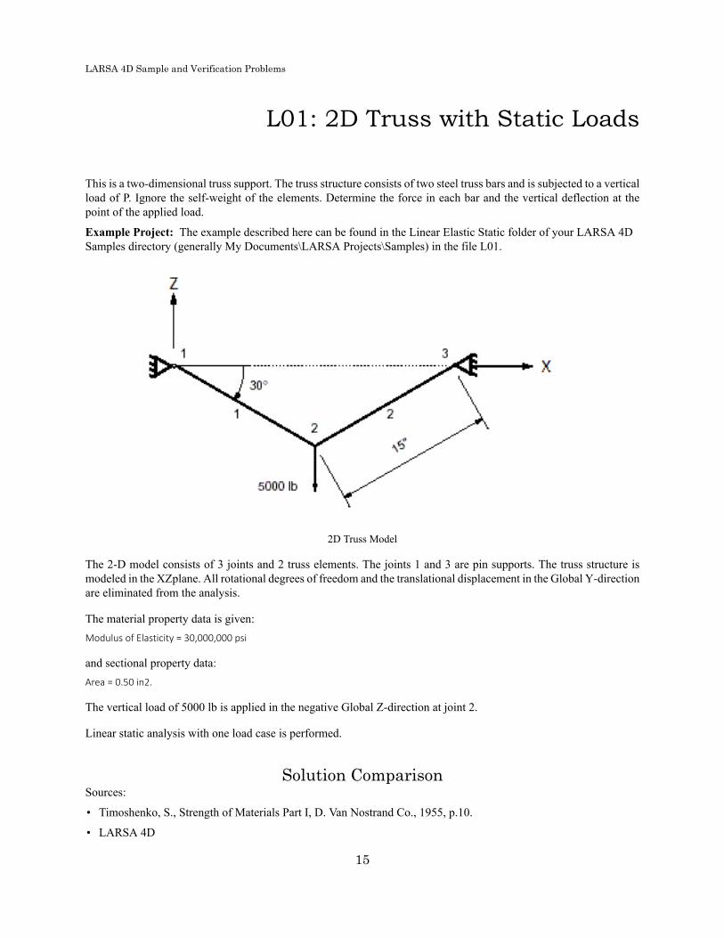
L01: 2D Truss with Static Loads
This is a two-dimensional truss support. The truss structure consists of two steel truss bars and is subjected to a verticalload of P. Ignore the self-weight of the elements. Determine the force in each bar and the vertical deflection at thepoint of the applied load.
Example Project: The example described here can be found in the Linear Elastic Static folder of your LARSA 4DSamples directory (generally My Documents\LARSA Projects\Samples) in the file L01.
2D Truss Model
The 2-D model consists of 3 joints and 2 truss elements. The joints 1 and 3 are pin supports. The truss structure ismodeled in the XZplane. All rotational degrees of freedom and the translational displacement in the Global Y-directionare eliminated from the analysis.
The material property data is given:Modulus of Elasticity = 30,000,000 psi
and sectional property data:Area = 0.50 in2.
The vertical load of 5000 lb is applied in the negative Global Z-direction at joint 2.
Linear static analysis with one load case is performed.
Solution ComparisonSources:
• Timoshenko, S., Strength of Materials Part I, D. Van Nostrand Co., 1955, p.10.
• LARSA 4D
15

LARSA 4D Sample and Verification Problems
Timoshenko LARSA
Axial Force @ I-end (lb) 5000 (Tension) -5000
Vertical Deflection @ 2(in) 0.12 (Down) -0.12
For More Information, please refer to the following documentation.
• For help on linear static analysis, see Linear Static Analysis in LARSA 4D Reference Manual.
16

LARSA 4D Sample and Verification Problems
L02: Beam with Elastic Supports
A two-span beam is supported at an interior point by a column and with yielding elastic supports at the two exteriorpoints. The beam is continuous and the column is pin-connected to the beam.
The beam is subjected to a vertical point load and the column is subjected to a horizontal point load. Determine thedeflections and reactions.
Example Project: The example described here can be found in the Linear Elastic Static folder of your LARSA 4DSamples directory (generally My Documents\LARSA Projects\Samples) in the file L02.
2D Model
The 2D model consists of 6 joints, 3 beam elements and 2 spring elements. This is a plane frame analysis. Thetranslational displacement in Global Y-direction and rotations about Global X and Z-directions can be deleted fromthe analysis. The joints 1, 4 and 6 are fixed supports.
The material property data is given:Modulus of Elasticity = 30,000,000 psi
and sectional property data:Area = 0.125 ft2
Izz = 0.263 ft4 for beams
Area = 0.175 ft2
Izz = 0.193 ft4 for columns
The spring constant for the springs is given as:k = 1200 kip/ft
The member loads applied on beams are:P = -15 kips on beam # 2 @ mid-span in Global Y
P = -5 kips on beam #3 @ mid-span in Global X
Linear static analysis with one load case is performed.
17

LARSA 4D Sample and Verification Problems
Solution ComparisonSources:
• Beaufait, F.W., et al., "Computer Methods of Structural Analysis," Prentice-Hall, 197-210.
• LARSA 4DBeaufait LARSA
U2 & U3 & U5 (x10^-3 ft) 1.079 1.079
V2 (x10^-3 ft) 1.7873 1.787
V3 (x10^-3 ft) -0.1803 -0.1803
V5 (x10^-3 ft) -4.8202 -4.8204
R2 (x10^-3 rad) 0.0992 0.0992
R3 (x10^-3 rad) -0.4443 -0.4443
R5 (x10^-3 rad) 0.3615 0.3615
Reaction V @ Joint 1 (kip) -2.1 -2.144
Reaction H @ Joint 4 (kip) -5.0 -5.0
Reaction V @ Joint 4 (kip) 11.3 11.360
Reaction M @ Joint 4 (kip) 30. 30.
Reaction V @ Joint 6 (kip) 5.8 5.7845
U denotes the displacement in horizontal direction and V denotes the displacement in vertical direction. R is therotation. Reaction V is the vertical force at the support joint and Reaction H is the horizontal force. Reaction M isthe support moment.
For More Information, please refer to the following documentation.
• For help on linear static analysis, see Linear Static Analysis in LARSA 4D Reference Manual.
18

LARSA 4D Sample and Verification Problems
L03: Beam on Elastic Foundation
A simply supported beam is uniformly loaded and is on an elastic foundation. The beam cross section is rectangularwith moment of inertia of 30 in^4. The elastic modulus of the beam is 30x10^6 psi. The span length is 240 inches. Theuniform load is 43.4 lb/in. The foundation modulus (i.e. distributed reaction for a deflection of unity) is 26.041667psi (lb/in^2).
Determine the transverse deflections and bending moments along the beam.
Example Project: The example described here can be found in the Linear Elastic Static folder of your LARSA 4DSamples directory (generally My Documents\LARSA Projects\Samples) in the file L03.
19

LARSA 4D Sample and Verification Problems
Beam on Elastic Foundation
The model consists of 21 joints, 20 beam elements and 19 grounded springs using a 2D model in the global XZ plane.The degrees of freedom for Y translation, X and Z rotations can be deleted from the analysis. Joint 1 is a pin supportand joint 21 is a roller support.
The material data is given as:Modulus of Elasticity = 30,000,000 lb/in^2
and sectional property data as:A = 7.11 in^2
Izz = 30 in^4
20

LARSA 4D Sample and Verification Problems
The member orientation angle is 90 degrees.
A distributed load of 43.4 lb/inch is applied in the vertical (Z)- direction as uniform beam load on all beam elements.Linear static analysis with one (1) load case is performed.
The foundation support is modeled using a set of foundation springs with stiffness of 312.50 lb/in in the vertical (Z)direction. The spring constant is computed as the product of the foundation modulus and tributary area for each joint.At all joints the tributary area is 12 inches (width of the beam) by 1 inch (unit length). Therefore, the spring constantfor a grounded spring element is:
k = (Foundation Modulus) x (Tributary Area)
k = (26.041667) x (12)
k = 312.50 lb/in
In this example, linear grounded spring elements are used and linear static analysis is performed. Since we know thesolution will yield the vertical displacement as downward with soil resistance active at all joints, we can use linearstatic analysis. However, the foundations can be subject to loads causing uplifts and loss of soil contact. It is moreappropriate to model the soil as compression-only foundation elements and perform nonlinear static analysis.
Solution ComparisonSources:
• Timoshenko, S. and Wionowsky-Krieger, S.,"Theory of Plates and Shells", McGraw-Hill Book Co., N.Y., 1959.
• "EASE2 - Elastic Analysis for Structural Engineering - Example Problem Manual," Engineering AnalysisCorporation, 1981, pp. 1.05.
• LARSA 4DTimoshenko EASE2 LARSA
Vertical Displacements
Station=0 0.0000 0.0000 0.0000
Station=12 -0.1693 -0.169 -0.1693
Station=24 -0.3331 -0.332 -0.3331
Station=36 -0.4870 -0.486 -0.4870
Station=48 -0.6270 -0.625 -0.6270
Station=60 -0.7502 -0.748 -0.7502
Station=72 -0.8541 -0.852 -0.8541
Station=84 -0.9367 -0.935 -0.9367
Station=96 -0.9967 -0.995 -0.9967
Station=108 -1.0331 -1.031 -1.0331
Station=120 -1.0453 -1.043 -1.0453
Bending Moment (lb-inch)
Station=0. 0 0
Station=6. 17872 17885
Station=18. 49247 49287
21
LARSA 4D Sample and Verification Problems
Timoshenko EASE2 LARSA
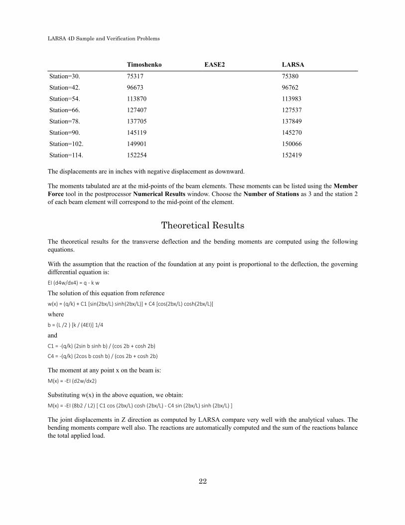
Station=30. 75317 75380
Station=42. 96673 96762
Station=54. 113870 113983
Station=66. 127407 127537
Station=78. 137705 137849
Station=90. 145119 145270
Station=102. 149901 150066
Station=114. 152254 152419
The displacements are in inches with negative displacement as downward.
The moments tabulated are at the mid-points of the beam elements. These moments can be listed using the MemberForce tool in the postprocessor Numerical Results window. Choose the Number of Stations as 3 and the station 2of each beam element will correspond to the mid-point of the element.
Theoretical ResultsThe theoretical results for the transverse deflection and the bending moments are computed using the followingequations.
With the assumption that the reaction of the foundation at any point is proportional to the deflection, the governingdifferential equation is:EI (d4w/dx4) = q - k w
The solution of this equation from referencew(x) = (q/k) + C1 [sin(2bx/L) sinh(2bx/L)] + C4 [cos(2bx/L) cosh(2bx/L)]
whereb = (L /2 ) [k / (4EI)] 1/4
andC1 = -(q/k) (2sin b sinh b) / (cos 2b + cosh 2b)
C4 = -(q/k) (2cos b cosh b) / (cos 2b + cosh 2b)
The moment at any point x on the beam is:M(x) = -EI (d2w/dx2)
Substituting w(x) in the above equation, we obtain:M(x) = -EI (8b2 / L2) [ C1 cos (2bx/L) cosh (2bx/L) - C4 sin (2bx/L) sinh (2bx/L) ]
The joint displacements in Z direction as computed by LARSA compare very well with the analytical values. Thebending moments compare well also. The reactions are automatically computed and the sum of the reactions balancethe total applied load.
22

LARSA 4D Sample and Verification Problems
For More Information, please refer to the following documentation.
• For help on linear static analysis, see Linear Static Analysis in LARSA 4D Reference Manual.
23

LARSA 4D Sample and Verification Problems
24
LARSA 4D Sample and Verification Problems
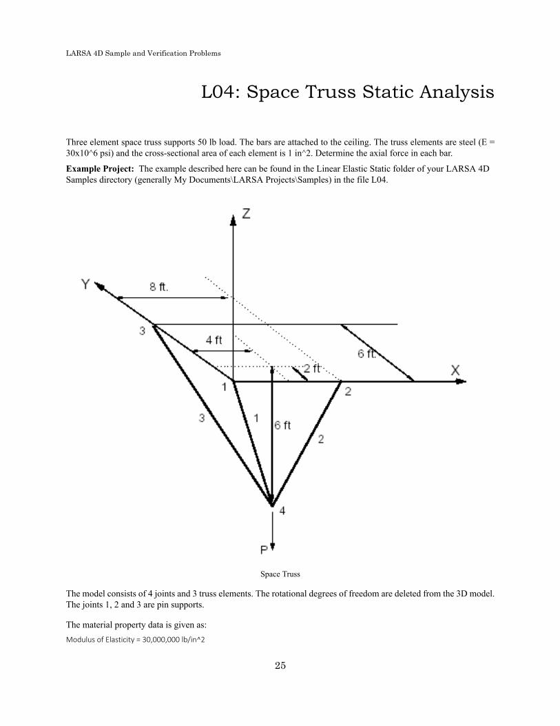
L04: Space Truss Static Analysis
Three element space truss supports 50 lb load. The bars are attached to the ceiling. The truss elements are steel (E =30x10^6 psi) and the cross-sectional area of each element is 1 in^2. Determine the axial force in each bar.
Example Project: The example described here can be found in the Linear Elastic Static folder of your LARSA 4DSamples directory (generally My Documents\LARSA Projects\Samples) in the file L04.
Space Truss
The model consists of 4 joints and 3 truss elements. The rotational degrees of freedom are deleted from the 3D model.The joints 1, 2 and 3 are pin supports.
The material property data is given as:Modulus of Elasticity = 30,000,000 lb/in^2
25

LARSA 4D Sample and Verification Problems
The sectional property data for the truss bar is:Area of each truss bar = 1 in^2
The load of 50 lb is applied in the vertical Global Z-direction. The applied load is:Load P @ Joint 4 in Z = -50 lb
Linear static analysis with one (1) load case is performed.
All truss elements are in tension.
Solution ComparisonSources:
• Beer, F.P., and Johnston, Jr., E.R., "Vector Mechanics for Engineers, Statics and Dynamics," McGraw-Hill BookCo., Inc. New York, 1962, p. 47.
• LARSA 4DBeer LARSA
Truss force F1 (lb) 10.4 10.4
Truss force F2 (lb) 31.2 31.2
Truss force F3 (lb) 22.9 22.9
For More Information, please refer to the following documentation.
• For help on linear static analysis, see Linear Static Analysis in LARSA 4D Reference Manual.
26

LARSA 4D Sample and Verification Problems
L05: 2D Truss with Thermal Load
This is a two dimensional truss structure with 32 feet height and 96 feet span. The top chord of the truss is subjectedto temperature rise of 50 degrees Fahrenheit. The coefficient of thermal expansion for the material is 0.0000065 in/in/F. The elastic modulus is 30,000,000 psi. Determine the member forces in the structure.
Example Project: The example described here can be found in the Linear Elastic Static folder of your LARSA 4DSamples directory (generally My Documents\LARSA Projects\Samples) in the file L05.
Joints and Members for 2D Truss Model
The material properties of the truss are given as:Modulus of Elasticity = 30,000,000 lb/in2
Coefficient of Thermal Expansion = 0.0000065 in/in/oF
The sectional properties are:Area = 24 in2 Designation = S1 Top & Bottom
Area = 32 in2 Designation = S2 Vertical Bars
Area = 40 in2 Designation = S3 Diagonal Bars
The truss model has 8 joints and 12 truss elements. The rotations (about X, Y and Z) and translation in Y-direction areeliminated. Joint 1 is pin support and joint 8 is a roller in horizontal direction.
The temperature rise on the top chord is specified for elements 13 and 14.
Solution ComparisonSources:
27

LARSA 4D Sample and Verification Problems
• Hsieh, Y.Y., "Elementary Theory of Structures," Prentice-Hall, Inc., 1970, pp. 200-202.
• LARSA 4DHsieh LARSA
F1,F2 0.00 0.00
F3 -21.1 -21.06
F4,F5,F6,F7 0.00 0.00
F8 -28.1 -28.08
F9 +35.1 +35.1
F10 +35.1 +35.1
F11 -28.1 -28.08
F12,F13 0.00 0.00
F14 -21.1 -21.06
Tensile force has positive magnitude. All forces are in kips.
For More Information, please refer to the following documentation.
• For help on linear static analysis, see Linear Static Analysis in LARSA 4D Reference Manual.
28

LARSA 4D Sample and Verification Problems
L06: Static Analysis of a SpaceFrame
A space frame having three members and four joints is subjected to static force loading. Points A and D are fullyrestrained. All members have the same cross-sectional properties. The loads on the frame consist of a force 2P in thepositive X direction at point B, a force P in the negative Y direction at point C, and a moment PL in the negative Zsense at C. Determine the final displaced shape of the structure. Include the effect of shearing deformations.
E = 200 x 106 kN/m2
G = 80 x 106 kN/m2
L = 3m
A = 0.01m2
Ixx = 2 x 10⁻³m4
Izz = Iyy = 1 x 10⁻³m4
P = 60 kN
Example Project: The example described here can be found in the Linear Elastic Static folder of your LARSA 4DSamples directory (generally My Documents\LARSA Projects\Samples) in the file L06.
29

LARSA 4D Sample and Verification Problems
Geometry and Loading
30

LARSA 4D Sample and Verification Problems
Joints and Members
ux,1[m] uy,1[m] uz,1[m] rotx,1[rad] roty,1[rad] rotz,1[rad]
Reference -0.859E-03 0.578E-04 0.501E-02 0.239E-02 -0.162E-02 0.681E-03
IDARC -0.859E-03 0.578E-04 0.501E-02 0.239E-02 -0.162E-02 0.681E-03
Difference None None None None None None
Fx,1[kN] Fy,1[kN] Fz,1[kN] Mx,1[kNm] My,1[kNm] Mz,1[kNm]
Reference 105.548 -38.509 -126.013 29.464 86.569 -67.100
IDARC 105.548 -38.509 -126.013 29.464 86.569 -67.100
Difference None None None None None None
Solution ComparisonSources:
• Weaver, Gere, Weaver Jr., Matrix Analysis of Framed Structures, 1990, p.354.
• Reinhorn, Simenonov, Mylonakis, Reichman, IDARC-BRIDGE: A computational Platform for Seismic DamageAssessment of Bridge Structures, MCEER, 1998, p.113.
• LARSA 4D
31

LARSA 4D Sample and Verification Problems
For More Information, please refer to the following documentation.
• For help on linear static analysis, see Linear Static Analysis in LARSA 4D Reference Manual.
32

LARSA 4D Sample and Verification Problems
L07: Plate Thermal Analysis
An equilateral triangular plate is simply supported at the edges. The plate is subjected to temperature variation along thethickness. The variation of temperature from top to bottom is 450o F. The coefficient of thermal expansion is 0.000012in/in/oF. The material elastic modulus and Poisson's Ratio are 10,000,000 psi and 0.30 respectively. Determine thedeflections along the base which is on X-axis.
Example Project: The example described here can be found in the Linear Elastic Static folder of your LARSA 4DSamples directory (generally My Documents\LARSA Projects\Samples) in the file L07.
Joints and Shell Elements for Triangular Plate
Due to the symmetry, half of the plate is taken for the model. The model has 36 joints and 28 plate elements.
The edges from joint 1 to 36 and 8 to 36 are the simply supported edges. The restraints for the joints from 1 to 8 arespecified to preserve the symmetry of the plate.
Linear static analysis with one (1) load case is performed.Modulus of Elasticity = 10,000,000 psi
Poisson's Ratio = 0.30
Shear Modulus = 3,841,615 psi
Coefficient of Thermal Expansion = 0.000012 in/in/oF
Plate Thickness = 0.10 inch
Temperature Gradient = 450o F for 0.10 inch thickness
33

LARSA 4D Sample and Verification Problems
The temperature gradient is the change of temperature for the unit thickness of the plate. The variation through 0.10inches is 450 o F, then for one inch thick (unit thickness), the temperature gradient is 4500 o F.
Solution ComparisonSources:
• Maulbetsch, J.L., "Thermal Stresses in Plates", Journal of Applied Mechanics, Vol. 57, June 1935, pp. A141-A146.
• LARSA 4DMaulbetsch LARSA
Ux @ x = 0.403 (in) 0.01590 0.01586
Ux @ x = 0.836 (in) 0.02290 0.02287
Ux @ x = 1.269 (in) 0.02224 0.02224
Ux @ x = 1.702 (in) 0.01677 0.01678
Ux @ x = 2.135 (in) 0.00934 0.00937
Ux @ x = 2.568 (in) 0.00280 0.00283
For More Information, please refer to the following documentation.
• For help on linear static analysis, see Linear Static Analysis in LARSA 4D Reference Manual.
34

LARSA 4D Sample and Verification Problems
L08: Shell-Bending of a TaperedCantilever
A tapered beam of rectangular cross-section is subjected to a load P at its tip. The beam is steel with 20 inches of span.The load P is 10 lbs. Determine the maximum deflection and the stress using shell elements.
Example Project: The example described here can be found in the Linear Elastic Static folder of your LARSA 4DSamples directory (generally My Documents\LARSA Projects\Samples) in the file L08.
Tapered Beam Model with Shell Elements
35

LARSA 4D Sample and Verification Problems
The model has 15 joints and 13 plate elements. The 3-node (triangular) plate elements are used in the model. Thejoints 8 and 18 are fixed supports.
Linear static analysis with one (1) load case is performed.
Modulus of Elasticity = 30,000,000 psi
Poisson's Ratio = 0.0
G = 15,000,000 psi
Plate Thickness = 0.50 inches
Span = 20 inches
P = 10 lb. (applied in the negative Z direction at joint 1)
Solution ComparisonSources:
• Harris, p. 114, problem 61.
• LARSA 4DHarris LARSA
Deflection (in) -0.04267 -0.04323
Moment (lb-in/in) 66.66 68.67
Stress (psi) 1600. 1648.
The section modulus of the plate is 0.04167 in3. The stress is computed using the following relationship:s = M / S
where
M = Bending moment
S = Section modulus
For More Information, please refer to the following documentation.
• For help on linear static analysis, see Linear Static Analysis in LARSA 4D Reference Manual.
36

LARSA 4D Sample and Verification Problems
L10: Tie Beam without GeometricStiffening
A tie beam is subjected to the action of a tensile force and a uniform lateral load. The tensile force is 21,970 lbs andthe uniform lateral load is 1.79253 lb/in. The beam is steel and has a square section of 2.5 in by 2.5 in. Determine themaximum deflection, maximum bending moment and the slope at the lefthand support.
Example Project: The example described here can be found in the Linear Elastic Static folder of your LARSA 4DSamples directory (generally My Documents\LARSA Projects\Samples) in the file L10.
Significance of geometric stiffening becomes evident when the results of the linear static analysis and nonlinear staticanalysis (Sample Problem N01) are compared.
Tie Beam Geometry and Loading
The model used has 9 joints and 8 beam elements. The tensile force is specified as an external joint force acting atjoint 9. The uniform load is specified as an external beam loading.
The data given for the problem is:Modulus of Elasticity = 30,000,000 lb/in2
Span = 200 inches
A = 6.25 in2
Izz = 3.2552 in4
Uniform Load = 1.79253 lb/in (applied as beam load)
Tensile Force S = 21,970 lb (applied at joint 9 in X)
37

LARSA 4D Sample and Verification Problems
Linear static analysis with one (1) load case is performed.
Solution ComparisonSources:
• Timoshenko, S.,"Strength of Materials, Part II", 3rd Edition, D. Van Nostrand Co., Inc., New York, p. 42.
• LARSA 4DTimoshenko LARSA
Vertical Disp @ Joint 5 (in) -0.382406 -0.382407
Rotation @ Joint 1 (rad) -0.0061185 -0.00611852
Moment @ I-end of Beam 5 (in-lb) -8962.65 -8962.65
The linear static analysis ignores the geometric stiffening effect of the beam. For comparison of the results to thenonlinear static analysis, refer to Problem 11.
For More Information, please refer to the following documentation.
• For help on linear static analysis, see Linear Static Analysis in LARSA 4D Reference Manual.
38

LARSA 4D Sample and Verification Problems
L11: Circular Plate with a HoleStatic Analysis
A circular plate with a center hole is built-in along the inner edge (i.e. fixed). The plate is subjected to bending by amoment applied along the outer edge. Determine the maximum deflection and slope of the plate. Also determine themoment near the inner and outer edges.
Example Project: The example described here can be found in the Linear Elastic Static folder of your LARSA 4DSamples directory (generally My Documents\LARSA Projects\Samples) in the file L11.
Circular Plate with a Hole
The circular plate is axisymmetric and only a small sector of the complete plate is needed for the analysis. We will usea 10 degree segment for approximating the circular boundary with a straight edge.
The model has 14 joints and 6 shell elements. The joints are numbered from 1 to 7 and 11 to 17. The plate elementsare 4-node elements.
39

LARSA 4D Sample and Verification Problems
The uniform moment of 10 in-lb/in is equivalent to a total moment of 52.3598 in-lb for the 10 degree segment. Themoment is applied at joints 7 and 17 as joint loads with magnitude of My = -26.1799387 in-lb. Linear static analysiswith one load case is performed.
Modulus of Elasticity = 30,000,000 psi
Poisson's Ratio = 0.30
Shear Modulus = 11,538,461 psi
Plate Thickness = 0.25 inches
Radius (inner) = 10 inches
Radius (outer) = 30 inches
The model is defined using cylindrical coordinates with R, Q and Z. The joints 1 to 7 are at Q = -5 degrees and 11 to17 are at Q = +5 degrees. The joint displacement directions are also defined in cylindrical R, Q and Z directions.
The model is created in LARSA 4D using the Classic and MITC4 plate element behaviors.
Solution ComparisonDisplacement at the outer edge and bending moment at the indicated locations are compared. In LARSA 4D, themoments are taken from the center of the nearest plate.
Result Timoshenko Classic MITC4
Rotation (rad) 0.0490577 0.04933 0.04910
Deflection (in) -0.0045089 -0.0045044 -0.0045104
M (x=10.86) (in-lb/in) -13.74 -13.12 -13.15
M (x=27.2) (in-lb/in) -10.12 -10.06 -10.11
References• Timoshenko, S.,"Strength of Materials, Part II", 3rd Edition, D. Van Nostrand Co., Inc., New York, p. 111.
For More Information, please refer to the following documentation.
• For help on linear static analysis, see Linear Static Analysis in LARSA 4D Reference Manual.
40

LARSA 4D Sample and Verification Problems
L12: Hemispherical Shell StaticAnalysis
A hemispherical shell is subjected to point loads at the lower two edges. The shell is 0.04 inches thick and the radiusis 10.0 inches. The modulus of elasticity is 6.825x10⁷ and Poisson's Ratio 0.30.
The top of the sphere is open at a vertical elevation of 9.511 inches. The elevation of the opening corresponds to anangle of 72 degrees when measured from the vertical axis Z.
Determine the displacement at the point of application of loads at joints 1 and 74.
Example Project: The example described here can be found in the Linear Elastic Static folder of your LARSA 4DSamples directory (generally My Documents\LARSA Projects\Samples) in the file L12.
Hemispherical Shell Mesh
41

LARSA 4D Sample and Verification Problems
A quarter of the hemispherical shell is used as a model. The model consists of 8 x 8 mesh of shell elements with thehorizontal mesh of 11.25 degrees and the vertical mesh of 9 degrees.
FE Model Nodes
The boundary conditions are prescribed for the symmetry. The joints along the edge from joint 1 to 9 are restrainedfor translation in the Global Y-direction and for rotations about Global X and Z-directions. Similarly, the joints alongthe edge from joint 74 to 82 are restrained for translation in the Global X-direction and for rotations about the GlobalY and Z-directions. Joint 38 at the lower center of the free edge is restrained to prevent unstable solution.
The geometry, material and section property data of the shell is:
Modulus of Elasticity = 68,250,000 psi
Poisson's Ratio = 0.30
Shear Modulus = 26,250,000 psi
Shell Thickness = 0.04 inch
Radius of the Hemisphere = 10 inch
42
LARSA 4D Sample and Verification Problems
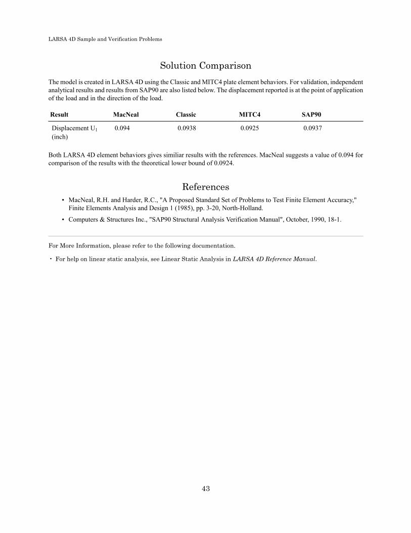
Solution ComparisonThe model is created in LARSA 4D using the Classic and MITC4 plate element behaviors. For validation, independentanalytical results and results from SAP90 are also listed below. The displacement reported is at the point of applicationof the load and in the direction of the load.
Result MacNeal Classic MITC4 SAP90
Displacement U1(inch)
0.094 0.0938 0.0925 0.0937
Both LARSA 4D element behaviors gives similiar results with the references. MacNeal suggests a value of 0.094 forcomparison of the results with the theoretical lower bound of 0.0924.
References• MacNeal, R.H. and Harder, R.C., "A Proposed Standard Set of Problems to Test Finite Element Accuracy,"
Finite Elements Analysis and Design 1 (1985), pp. 3-20, North-Holland.
• Computers & Structures Inc., "SAP90 Structural Analysis Verification Manual", October, 1990, 18-1.
For More Information, please refer to the following documentation.
• For help on linear static analysis, see Linear Static Analysis in LARSA 4D Reference Manual.
43

LARSA 4D Sample and Verification Problems
44
LARSA 4D Sample and Verification Problems
L13: Cylindrical Roof Static Analysis
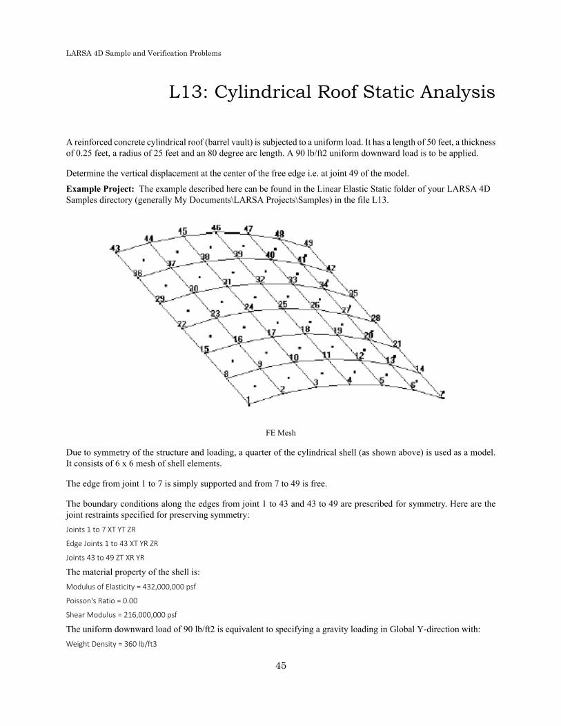
A reinforced concrete cylindrical roof (barrel vault) is subjected to a uniform load. It has a length of 50 feet, a thicknessof 0.25 feet, a radius of 25 feet and an 80 degree arc length. A 90 lb/ft2 uniform downward load is to be applied.
Determine the vertical displacement at the center of the free edge i.e. at joint 49 of the model.
Example Project: The example described here can be found in the Linear Elastic Static folder of your LARSA 4DSamples directory (generally My Documents\LARSA Projects\Samples) in the file L13.
FE Mesh
Due to symmetry of the structure and loading, a quarter of the cylindrical shell (as shown above) is used as a model.It consists of 6 x 6 mesh of shell elements.
The edge from joint 1 to 7 is simply supported and from 7 to 49 is free.
The boundary conditions along the edges from joint 1 to 43 and 43 to 49 are prescribed for symmetry. Here are thejoint restraints specified for preserving symmetry:Joints 1 to 7 XT YT ZR
Edge Joints 1 to 43 XT YR ZR
Joints 43 to 49 ZT XR YR
The material property of the shell is:Modulus of Elasticity = 432,000,000 psf
Poisson's Ratio = 0.00
Shear Modulus = 216,000,000 psf
The uniform downward load of 90 lb/ft2 is equivalent to specifying a gravity loading in Global Y-direction with:Weight Density = 360 lb/ft3
45

LARSA 4D Sample and Verification Problems
For a shell thickness of 0.25 ft and weight density of 360 lb/ft3, this combination gives the desired 90 lb/ft2 uniformloading in Global Y-direction.
The input for the model should be generated using a cylindrical coordinate system.
Reference• MacNeal, R.H. and Harder, R.C., "A Proposed Standard Set of Problems to Test Finite Element Accuracy,"
Finite Elements in Analysis and Design 1 (1985), pp.3-20, North-Holland.
• Zienkiewicz, O. C., "The Finite Element Method," McGraw-Hill, 1977.
Solution ComparisonSources:
• Computers & Structures Inc., "SAP90 Structural Analysis Verification Manual", October, 1990, 16-1.
• Theory
• LARSA 4DSAP90 Theory LARSA
Axial Z-Displacement infeet at the Support Joints1-7
Location=0.00(deg) 0.0000 0.0004 0.0000
Location=6.67(deg) 0.0005 0.0009 0.0005
Location=13.33(deg) 0.0018 0.0020 0.0018
Location=20.00(deg) 0.0029 0.0030 0.0029
Location=26.67(deg) 0.0024 0.0021 0.0024
Location=33.33(deg) -0.0017 -0.0016 -0.0017
Location=40.00(deg) -0.0118 -0.0120 -0.0118
Vertical Y-Displacementin feet at the Center Joints43-49
Location=0.00(deg) 0.046 0.045 0.047
Location=6.67(deg) 0.031 0.027 0.031
Location=13.33(deg) -0.013 -0.018 -0.013
Location=20.00(deg) -0.078 -0.082 -0.079
Location=26.67(deg) -0.155 -0.155 -0.157
Location=33.33(deg) -0.234 -0.241 -0.236
Location=40.00(deg) -0.307 -0.309 -0.309
Moments Mx (lb-ft/ft) atthe Central Section Shell31-36
Location=3.33(deg) -2038 -2045 -2004
46

LARSA 4D Sample and Verification Problems
SAP90 Theory LARSA
Location=10.00(deg) -1796 -1810 -1772
Location=16.67(deg) -1329 -1310 -1321
Location=23.33(deg) -727 -715 -730
Location=30.00(deg) -186 -165 -192
Location=36.67(deg) 14 +25 16
Twisting Moments Mxy(lb-ft/lb) at the SupportShell 1-6
Location=3.33(deg) -225 -190 -177
Location=10.00(deg) -529 -525 -520
Location=16.67(deg) -840 -835 -828
Location=23.33(deg) -1082 -1120 -1063
Location=30.00(deg) -1215 -1265 -1187
Location=36.67(deg) -1241 -1265 -1198
The midside vertical displacement computed by LARSA is -0.309 feet agreeing well with the theoretical value of-0.309.
Important note: The bending and twisting moments from the Reference and theory are reported for the edge of theplate whereas the values from LARSA are at the center of each plate element. Since the bending and twisting momentsare expected to be slightly lower at the center (about 2 feet from the edge) of the plate than the values at the edge, theresults from LARSA are agreeing well with theory and Reference.
For More Information, please refer to the following documentation.
• For help on linear static analysis, see Linear Static Analysis in LARSA 4D Reference Manual.
47

LARSA 4D Sample and Verification Problems
48

LARSA 4D Sample and Verification Problems
L14: 2D Truss - Thermal Loads andSettlement
2D truss shown below is subjected to various loads. In case 1, the truss is subjected to a uniform temperature rise of70 degrees Fahrenheit. In case 2, concentrated forces of 10,000 lb. each are applied at the joints of the top chord ofthe truss. In addition to applied loads, the right support undergoes some settlement relative to the support. The verticalsettlement is 0.01 ft down and the horizontal settlement is 0.01 ft towards right. In case 2, the temperature drops 40degrees F.
Calculate the vertical deflection at the top hinge (at Joint 5).
Example Project: The example described here can be found in the Linear Elastic Static folder of your LARSA 4DSamples directory (generally My Documents\LARSA Projects\Samples) in the file L14.
2D Truss and FE Model Joints
The material properties for the truss bars are:Modulus of Elasticity = 30,000,000 psi
Coefficient of Thermal Expansion = 0.0000065
The section property for the truss bars is:Axx = 2.0 in2
The finite element model consists of 14 truss elements. Linear static analysis is performed with 2 primary load cases.
49

LARSA 4D Sample and Verification Problems
Solution ComparisonTranslational displacement in global direction at Joint 5 (in feet):Sources:
• Timoshenko, S.P. and Young, D.H., "Theory of Structures,", 2nd ed., McGraw-Hill, New York, 1965, pp.266-267.
• LARSA 4DTimoshenko LARSA
Load Case 1 +0.158 +0.158
Load Case 2 -0.223 -0.223
The comparison of the results is excellent.
For More Information, please refer to the following documentation.
• For help on linear static analysis, see Linear Static Analysis in LARSA 4D Reference Manual.
50

LARSA 4D Sample and Verification Problems
L16: Nonlinear Thermal Load
The three-span continous concrete beam is subjected to a thermal load that is uniform along the length of the memberbut varies along the vertical axis of the cross-section. The nonlinear variation causes self-equilibriating stresses.
Example Project: The example described here can be found in the Linear Elastic Static folder of your LARSA 4DSamples directory (generally My Documents\LARSA Projects\Samples) in the file L16.
The three-span continous concrete beam in the figure below is subjected to a nonlinear thermal gradient. The memberhas a T-shaped cross-section (1.6m depth, 2.8 m width, 0.4 m web thickness, 0.2 m flange thickness). The materialhas a modulus of elasticity of 3x10⁸ N/m2 and a coefficient of thermal expansion of 10x10-6 1/°C.
The spans are 21 m, 27 m, and 21 m.
The thermal load is uniform along the length of the member but it varies as a fifth-order parabola along the depth ofthe section, from a maximum of 25°C at the top fiber to 0°C at a depth of 1.2 m and below. The temperature changeas a function of depth, measured from the top of the section, is given by the equation:ΔT = 4.21 × 25 × ((3/4 - y/1.6)^5) (°C)
for y < 1.2 m, and ΔT = 0 in 1.2 m <= y <= 1.6 m.
The nonlinear gradient creates self-equilibriating stresses.
Calculate the total stress at a fiber.
The model, cross-section, and thermal gradient are depicted in the figure below:
3-Span Beam, X-Section and Temperature Variation
Solution ComparisonStress at the top fiber, centroid, and bottom fiber (at mid-span locations) are reported in the table below. Units areN/mm2.Sources:
51

LARSA 4D Sample and Verification Problems
• Structural Analysis 4th edition, example 5-3, page 132. A. Ghali and A.M. Neville.
• LARSA 4DGhali LARSA
Top Fiber -5.20 MPa -5.19 MPa
Centroid 2.16 MPa 2.17 MPa
Bottom Fiber 3.49 MPa 3.50 MPa
The comparison of the results is excellent.
For More Information, please refer to the following documentation.
• For help on linear static analysis, see Linear Static Analysis in LARSA 4D Reference Manual.• For help on member thermal loads, see Member Thermal Loads in LARSA 4D Reference Manual.
52

LARSA 4D Sample and Verification Problems
L17: Plane Stress Element-StraightBeam with Static Loads
A straight cantilever beam, modeled with plane stress elements, is subjected to unit forces at the tip in the X andY directions and a unit moment at the tip about the Y direction, each in a different load case. Please note that thisexample is an extreme case presented for testing and verification of the plane plate elements. Plane plate elements arenot in general intended for use in modeling a beam with a 2 to 1 depth-to-width ratio. The problem is modeled withclassic, bilinear, drilling and incompatible plates with different mesh sizes. The solutions are compared to independentsolutions from MacNeal and Harder 1985.
Example Project: The example described here can be found in the LinearStatic folder of your LARSA 4D Samplesdirectory (generally My Documents\LARSA Projects\Samples) in the file L17.
Problem DescriptionThe basic geometry, properties and loadings are as described in MacNeal and Harder 1985. The cantilever beam is 6inches long, 0.2 inch wide parallel to the Z direction, and 0.1 inch wide parallel to the Y direction. For testing elementswith incompatible bending modes and drilling degrees of freedom, three different models meshed with six elementsare used as suggested in MacNeal and Harder 1985. Model A uses rectangular elements, model B uses trapezoidalelements, and model C uses parallelogram elements. For testing classic and bilinear plates, a triangular model, modelD, with 12 triangle elements is added to the mix.
Model Diagrams
Material properties of the cantilever beam, namely the elastic modulus E and Poisson's ratio v are defined as follows:
E = 10,000,000 lb/in2
v = 0.3
LoadingThree load cases are created for each model, applying a unit axial force, a unit in-plane force, and a unit in-planemoment at the tip of the cantilever, respectively. The in-plane moment is applied as a couple of forces in the X direction.
The independent solution is derived using elementary beam theory that assumes no local Poisson's effect occurring atthe support. The beam is modeled to match this assumption by applying an in-plane force equal to the applied tip loadin the opposite direction to model the reaction without Poisson's effect.
In the LARSA 4D models the Ux and Uz degrees of freedom are active; all other degrees of freedom are inactive.For models with drilling plates rotations in Ry direction are set active as drilling elements have this rotation degreeof freedom. At the fixed end, joint 1 is restrained in the Ux and Uz degrees of freedom and joint 8 is restrained in theUx degrees of freedom only. Joint 8 is not restrained in the Uz degrees of freedom to avoid imposing the unwantedlocal Poisson's effect on the model.
53

LARSA 4D Sample and Verification Problems
Load Case Load Type Load
1 Axial Extension Fx = +0.5 lb at joints 7 and 14
2 In-Plane Shear and Bending Fz = +0.5 lb at joints 7 and 14 Fz =-0.5 lb at joint 8
3 In-Plane Moment Fx = -5 lb at joint 7 Fx = +5 lb atjoint 14
Solution Comparison
Plates with Incompatible Bending Modes
First, models A, B, and C are modeled with plate elements with the incompatible membrane type. The following tablepresents the results of solutions to these models and their comparisons to the independent results.
Comparison of Solutions of Models A-C using Plates withIncompatible Bending Modes for Different Mesh Sizes
Load Type Model andElement Shape
OutputParameter
Independent LARSA4D PercentDifference
Axial Extension A - Rectangle Ux @ Joint 14 3.000E-05 3.00E-05 0%
Axial Extension B - Trapezoid Ux a@ Joint 14 3.000E-05 3.00E-05 0%
Axial Extension C -Parallelogram
Ux @ Joint 14 3.000E-05 3.00E-05 0%
In-PLane Shearand Bending
A - Rectangle Uxz @ Joint 14 0.1081 0.1073 0.7%
In-Plane Shearand Bending
B - Trapezoid Ux @ Joint 14 0.1081 0.0247 77.1%
In-Plane Shearand bending
C -Parallelogram
Ux @ Joint 14 0.1081 0.0874 19.1%
In-PlaneMoment
A - Rectangle Ux @ Joint 14 9.000E-04 0.00090 0%
In-PlaneMoment
B - Trapezoid Ux @ Joint 14 9.000E-04 0.000015 98.3%
In-PlaneMoment
C -Parallelogram
Ux @ Joint 14 9.000E-04 0.00076 91.5%
Model A which uses rectangular elements with the incompatible bending modes membrane type gives close resultsto the independent solutions in all load cases. However models B and C get close to the independent solution onlyin the axial extension load case.
54

LARSA 4D Sample and Verification Problems
Accurate results can be obtained from these models by breaking the trapezoidal elements into smaller ones. Smallertrapezoidal elements will have straighter angles between opposite edges and the aspect ratio of these elements will becloser to one. First we break the first and last elements of models B and C to see if the trapezoidal elements are theproblem and parallelogram elements work correctly.
The following table presents the solutions of models B and C with or without breaking the first and last trapezoidalelements and their comparisons to the independent solutions. In the models with broken elements, named F-L, the firstand the last trapezoidal elements are broken into four smaller ones. If we break the first and last elements of ModelB, the trapezoidal model, we get better results than the unbroken case. However the results are not close proximityto the independent solutions. If break the first and last elements of Model C, the parallelogram model, we get betterresults than the unbroken case and the results are close to the independent solutions. This confirms that the shape oftrapezoidal elements are the problem and not the shape of parallelogram elements.
Comparison of Solutions of Models B and C with or without Breaking of Trapezoidal Elements
In-PLane Shear andBending
In-Plane Moment
LARSA 4D Percent Difference LARSA 4D Percent Difference
B - Trapezoid 6x1 2.47E-02 -77.1% 1.54E-04 -82.9%
B - Trapezoid F-L 4.93E-02 -54.4% 3.25E-04 -63.9%
C - Parallelogram6x1
8.75E-02 -19.1% 7.68E-04 -14.7%
C - Parallelogram F-L
1.08E-01 -0.2% 9.02E-04 -0.1%
If break all elements of model B into 4 trapezoids, we can achieve close proximity to the independent solution. Thefollowing table presents the comparison of results for model B meshed into 96 elements to model B meshed into 6elements. The finely meshed model gives close proximity results to the independent solutions, showing the importanceof the shapes of trapezoidal elements.
Comparison of Solutions of Model B for Course (6x1) and Fine (24x1) Meshes
In-PLane Shear andBending
In-Plane Moment
LARSA 4D Percent Difference LARSA 4D Percent Difference
B - Trapezoid 6x1 2.47E-02 -77.1% 1.54E-04 -82.9%
B - Trapezoid 24x1 1.08E-01 0.1% 9.01E-04 0.1%
Plates With Drilling Degrees of Freedoms
The following tables summarizes the results and their differences from the independent solutions, for models A, B, Csolved using plates with the drilling membrane type. Results for models with different mesh sizes are also presentedto show the effects of element size.
For axial extension all models provide correct results. For in-plane shear and bending and in-plane moment onlyrectangular elements can get close to 2% range of independent solutions. For all element geometries increasing mesh
55
LARSA 4D Sample and Verification Problems
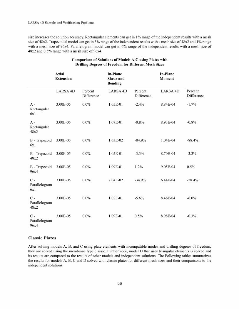
size increases the solution accuracy. Rectangular elements can get in 1% range of the independent results with a meshsize of 48x2. Trapezoidal model can get in 3% range of the independent results with a mesh size of 48x2 and 1% rangewith a mesh size of 96x4. Parallelogram model can get in 6% range of the independent results with a mesh size of48x2 and 0.5% range with a mesh size of 96x4.
Comparison of Solutions of Models A-C using Plates withDrilling Degrees of Freedom for Different Mesh Sizes
AxialExtension
In-PlaneShear andBending
In-PlaneMoment
LARSA 4D PercentDifference
LARSA 4D PercentDifference
LARSA 4D PercentDifference
A -Rectangular6x1
3.00E-05 0.0% 1.05E-01 -2.4% 8.84E-04 -1.7%
A -Rectangular48x2
3.00E-05 0.0% 1.07E-01 -0.8% 8.93E-04 -0.8%
B - Trapezoid6x1
3.00E-05 0.0% 1.63E-02 -84.9% 1.04E-04 -88.4%
B - Trapezoid48x2
3.00E-05 0.0% 1.05E-01 -3.3% 8.70E-04 -3.3%
B - Trapezoid96x4
3.00E-05 0.0% 1.09E-01 1.2% 9.05E-04 0.5%
C -Parallelogram6x1
3.00E-05 0.0% 7.04E-02 -34.9% 6.44E-04 -28.4%
C -Parallelogram48x2
3.00E-05 0.0% 1.02E-01 -5.6% 8.46E-04 -6.0%
C -Parallelogram96x4
3.00E-05 0.0% 1.09E-01 0.5% 8.98E-04 -0.3%
Classic Plates
After solving models A, B, and C using plate elements with incompatible modes and drilling degrees of freedom,they are solved using the membrane type classic. Furthermore, model D that uses triangular elements is solved andits results are compared to the results of other models and independent solutions. The Following tables summarizesthe results for models A, B, C and D solved with classic plates for different mesh sizes and their comparisons to theindependent solutions.
56

LARSA 4D Sample and Verification Problems
For axial extension all models provide correct results. For in-plane shear and bending and in-plane moment onlyrectangular meshes can give results close proximity to the independent solutions. The trapezoidal models give resultswithin 4% range of the independent results with a mesh size of 24x1 and within 1% range with a mesh size of 48x2.Similar to the models with incompatible bending modes, parallelogram models give better results than trapezoidalresults using classical plates. Parallelogram models can get in 1% range of independent solutions with a mesh size of24x1. Triangle models need considerably more elements to get in close range of independent solutions. A 96 elementmodel gets in 70% range and a 768 element model can get in 20% range.
Comparison of Solutions of Models A-D with Classic Plates for Different Mesh Sizes
AxialExtension
In-PlaneShear andBending
In-PlaneMoment
LARSA 4D PercentDifference
LARSA 4D PercentDifference
LARSA 4D PercentDifference
A -Rectangular6x1
3.00E-05 0% 1.07E-01 -1% 9.00E-04 0%
B - Trapezoid6x1
3.00E-05 0% 1.36E-02 -87% 9.18E-05 -90%
B - Trapezoid24x1
3.00E-05 0% 1.04E-01 -4% 8.64E-04 -4%
B - Trapezoid48x2
3.00E-05 0% 1.08E-01 0% 8.98E-04 0%
C -Parallelogram6x1
3.00E-05 0% 7.62E-02 -30% 6.95E-04 -23%
C -Parallelogram24x1
3.00E-05 0% 1.08E-01 -1% 8.96E-04 0%
C -Parallelogram48x2
3.00E-05 0% 1.08E-01 0% 8.98E-04 0%
D - Triangle12
3.00E-05 0% 2.82E-05 -100% 2.82E-05 -97%
D - Triangle96
3.00E-05 0% 3.23E-02 -70% 2.68E-04 -70%
D - Triangle768
3.00E-05 0% 8.70E-02 -20% 7.22E-04 -20%
57

LARSA 4D Sample and Verification Problems
Bilinear Plates
The following tables summarize the results for models A, B, C and D solved with bilinear plates for different mesh sizesand their differences from the independent solutions. For axial extension all models provide correct results. For in-plane shear and bending and in-plane moment none of the models can get in close proximity to the independent resultswith a mesh size of 6x1 for quad elements and 12 for triangular elements. However increasing mesh size increasesthe solution accuracy. Rectangular elements can get in 3% range of the independent results with a mesh size of 96x4.Trapezoidal model can get in 11% range of the independent results with a mesh size of 96x4. Parallelogram modelcan get in 20% range of the independent results with a mesh size of 96x4. Triangle models give similar results to thetriangles models with classic plates. A 96 element model gets in 70% range and a 768 element element model canget in 20% range.
Comparison of Solutions of Models A-D with Bilinear Plates for Different Mesh Sizes
AxialExtension
In-PlaneShear andBending
In-PlaneMoment
LARSA 4D PercentDifference
LARSA 4D PercentDifference
LARSA 4D PercentDifference
A -Rectangular6x1
3.00E-05 0% 1.01E-02 -91% 8.40E-05 -91%
A -Rectangular48x2
3.00E-05 0% 9.20E-02 -15% 7.66E-04 -15%
A -Rectangular96x4
3.00E-05 0% 1.05E-01 -3% 8.72E-04 -3%
B - Trapezoid6x1
3.00E-05 0% 2.99E-03 -97% 2.06E-05 -98%
B - Trapezoid48x2
3.00E-05 0% 7.33E-02 -32% 6.06E-04 -33%
B - Trapezoid96x4
3.00E-05 0% 9.74E-02 -10% 8.04E-04 -11%
C -Parallelogram6x1
3.00E-05 0% 3.77E-03 -97% 2.82E-05 -97%
C -Parallelogram48x2
3.00E-05 0% 5.72E-02 -47% 4.49E-04 -50%
C -Parallelogram96x4
3.00E-05 0% 8.84E-02 -18% 7.17E-04 -20%
58

LARSA 4D Sample and Verification Problems
AxialExtension
In-PlaneShear andBending
In-PlaneMoment
D - Triangle12
3.00E-05 0% 3.45E-03 -97% 2.82E-05 -97%
D - Triangle96
3.00E-05 0% 3.23E-02 -70% 2.68E-04 -70%
D - Triangle768
3.00E-05 0% 8.70E-02 -20% 7.22E-04 -20%
ConclusionIn this example, a plane cantilever beam subjected to axial, shear and bending, and moment loadings is modeled withdifferent plate types and different mesh sizes. Furthermore, models with different element geometries are used toobserve the effects of element shapes on the results. Results are compared to each other and solutions from independentsources.
The best results are achieved using plate elements with incompatible modes. Plates with incompatible modes arefollowed by classic plates, plates with drilling degrees of freedom and bilinear plates in terms of solution accuracy.
The shape of the element directly effects the accuracy of the results. For all plate types rectangular elements give themost accurate results. Furthermore, the more rectangular the element shape the better results are. For all plate types,quadrilateral element shapes give better results than triangular ones.Sources:
• Cook and Young, "Advanced Mechanics of Materials," 1985, pp. 244.
• MacNeal, R.H. and Harder, R.L., "A Proposed Standard Set of Problems to Test Finite Element Accuracy," Finite Elements Analysis and Design 1 (1985), pp. 3-20, North-Holland.
• SAP 2000, CSI Software Verification Example 3-002, "Plane-Straight Beam with Static Loads."
For More Information, please refer to the following documentation.
• For help on linear static analysis, see Linear Static Analysis in LARSA 4D Reference Manual.
59

LARSA 4D Sample and Verification Problems
60

LARSA 4D Sample and Verification Problems
L18: Shell-Straight Beam with StaticLoads
A straight cantilever beam, modeled with shell elements with different configurations, is subjected to unit forces andmoments at the tip in all orthogonal directions, each in a different load case. Tip deflections in the direction of loadingsare tracked and compared with analytical results as well as SAP2000's. Please note that this example is an extreme casefor testing shell elements since they are not intended for use in modeling a beam with a 2 to 1 depth-to-width ratio.
Example Project: The example described here can be found in the Linear Elastic Static folder ofyour LARSA 4D Samples directory (generally My Documents\LARSA Projects\Samples) in the fileL18_Rectangular_Thin_Incompatible_6x1.
Problem DescriptionThis problem is described in the paper "A Proposed Standard set of Problems to Tests Finite Element Accuracy" byMacNeal and Harder (1985). The cantilever beam has a length of 6 inches (in X direction), a depth of 0.2 inches (inZ direction) and a width of 0.1 inches (in Y direction). This geometry is modeled with five different meshes and eachmesh is excited with six different load cases. The meshes, loadings and material properties also conform to the papermentioned above.
Mesh models
First three models use quadrilateral elements with different geometric irregularities and last two model use triangularelements with a varying degree of fineness. All models are shown in following figure. Sign convention for axes, nodeand element labels are also given in the figure.
61

LARSA 4D Sample and Verification Problems
Mesh diagrams
Load cases
Six load cases are created for each model. These load cases apply a unit axial force, a unit in-plane force, unit out-of-plane force, a unit twisting moment, a unit in-plane moment and a unit out-of-plane moment at the tip of the
62

LARSA 4D Sample and Verification Problems
cantilever, respectively. The twisting moment is applied as a force couple in Y axis. The in-plane moment is appliedas a force couple in X axis. Only the out-of-plane moment is applied as moments. The details of the loadings are givenin following table.
Load Case Load Type Load
1 Axial extension Fx = +0.5 lb at joint 7 and 14
2 In-plane shear and bending Fz = +0.5 lb at joint 7 and 14, Fz =-0.5 lb at joint 8
3 Out-of-plane shear and bending Fy = +0.5 lb at joint 7 and 14
4 Twisting moment Fy = -5 lb at joint 7, Fy = +5 lb atjoint 14
5 In-plane moment Fx = -5 lb at joint 7, Fx = +5 lb atjoint 14
6 Out-of-plane moment Mz = +0.5 lb-in at joint 7 and 14
Material properties
E = 10,000,000 lb/in2
v = 0.3
G = 3,846,154 lb/in2
Shell thickness = 0.1 in
ResultsThe independent solution is derived using elementary beam theory that assumes no local Poisson's effect at the support.The beam is modeled to match this assumption in LARSA 4D. At the fixed end, joint 1 is restrained in the Ux, Uy, Uzand Rz degrees of freedom and joint 8 is restrained in the Ux, Uy and Rz degrees of freedom. Joint 8 is not restrainedin the Uz degree of freedom to avoid imposing unwanted local Poisson's effect into the model. Also, when the beamis loaded with in-plane shear, an in-plane force equal to half the applied tip load is applied to joint 8 in the oppositedirection of the tip load. This special load at joint 8 is applied to model the reaction without the Poisson's effect.
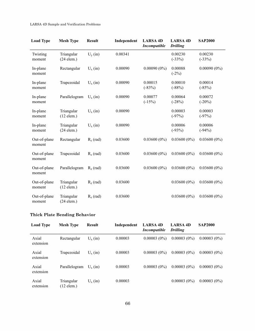
The results are compared for four LARSA 4D plate element behaviors: Classic, Thin Plate, Thick Plate, and MITC4.For the Thin and Thick Plate, the Incompatible and Drilling membrane behaiors are combined with the bendingbehavior and reported in separate columns. The bilinear membrane behavior and the MITC4 behavior are knownto suffer from the shear-locking phenomena which is relevant in the in-plane bending and moment load cases. Thebilinear membrane behavior is therefore not included in this comparison, and MITC4 results are only reported for outof plane load cases.
The results reported in SAP2000's corresponding document are also given. It is important to note that all results arethe averages of absolute values obtained from joints 7 and 14. The percentages in the parantheses next to the resultsindicate relative percentage errors.
63

LARSA 4D Sample and Verification Problems
Classic Element Behavior
Load Type Mesh Type Result Independent LARSA 4D
Axial extension Rectangular Ux (in) 0.00003 0.00003 (0%)
Axial extension Trapezoidal Ux (in) 0.00003 0.00003 (0%)
In-plane shear andbending
Rectangular Uz (in) 0.10810 0.10733 (-1%)
In-plane shear andbending
Trapezoidal Uz (in) 0.10810 0.01376 (-87%)
Out-of-plane shearand bending
Rectangular Uy (in) 0.43210 0.42864 (-1%)
Out-of-plane shearand bending
Trapezoidal Uy (in) 0.43210 0.41601 (-4%)
Twisting moment Rectangular Uy (in) 0.00341 0.00206 (-40%)
Twisting moment Trapezoidal Uy (in) 0.00341 0.00209 (-39%)
In-plane moment Rectangular Ux (in) 0.00090 0.00090 (0%)
In-plane moment Trapezoidal Ux (in) 0.00090 0.00009 (-90%)
Out-of-planemoment
Rectangular Rz (rad) 0.03600 0.03600 (0%)
Out-of-planemoment
Trapezoidal Rz (rad) 0.03600 0.03600 (0%)
Thin Plate Bending Behavior
Load Type Mesh Type Result Independent LARSA 4DIncompatible
LARSA 4DDrilling
SAP2000
Axialextension
Rectangular Ux (in) 0.00003 0.00003 (0%) 0.00003 (0%) 0.00003 (0%)
Axialextension
Trapezoidal Ux (in) 0.00003 0.00003 (0%) 0.00003 (0%) 0.00003 (0%)
Axialextension
Parallelogram Ux (in) 0.00003 0.00003 (0%) 0.00003 (0%) 0.00003 (0%)
Axialextension
Triangular(12 elem.)
Ux (in) 0.00003 0.00003 (0%) 0.00003 (0%)
Axialextension
Triangular(24 elem.)
Ux (in) 0.00003 0.00003 (0%) 0.00003 (0%)
64

LARSA 4D Sample and Verification Problems
Load Type Mesh Type Result Independent LARSA 4DIncompatible
LARSA 4DDrilling
SAP2000
In-planeshear andbending
Rectangular Uz (in) 0.10810 0.10733(-1%)
0.10548(-2%)
0.10720(-1%)
In-planeshear andbending
Trapezoidal Uz (in) 0.10810 0.02517(-77%)
0.01655(-85%)
0.02270(-79%)
In-planeshear andbending
Parallelogram Uz (in) 0.10810 0.08703(-19%)
0.07009(-35%)
0.08040(-26%)
In-planeshear andbending
Triangular(12 elem.)
Uz (in) 0.10810 0.00345(-97%)
0.00320(-97%)
In-planeshear andbending
Triangular(24 elem.)
Uz (in) 0.10810 0.00705(-93%)
0.00660(-94%)
Out-of-planeshear andbending
Rectangular Uy (in) 0.43210 0.43200 (0%) 0.43200 (0%) 0.43200 (0%)
Out-of-planeshear andbending
Trapezoidal Uy (in) 0.43210 0.43217 (0%) 0.43217 (0%) 0.43220 (0%)
Out-of-planeshear andbending
Parallelogram Uy (in) 0.43210 0.43219 (0%) 0.43219 (0%) 0.43220 (0%)
Out-of-planeshear andbending
Triangular(12 elem.)
Uy (in) 0.43210 0.42962(-1%)
0.42960(-1%)
Out-of-planeshear andbending
Triangular(24 elem.)
Uy (in) 0.43210 0.43137 (0%) 0.43140 (0%)
Twistingmoment
Rectangular Uy (in) 0.00341 0.00233(-32%)
0.00233(-32%)
0.00233(-32%)
Twistingmoment
Trapezoidal Uy (in) 0.00341 0.00233(-32%)
0.00233(-32%)
0.00233(-32%)
Twistingmoment
Parallelogram Uy (in) 0.00341 0.00233(-32%)
0.00233(-32%)
0.00233(-32%)
Twistingmoment
Triangular(12 elem.)
Uy (in) 0.00341 0.00231(-32%)
0.00231(-32%)
65
LARSA 4D Sample and Verification Problems
Load Type Mesh Type Result Independent LARSA 4DIncompatible
LARSA 4DDrilling
SAP2000
Twistingmoment
Triangular(24 elem.)
Uy (in) 0.00341 0.00230(-33%)
0.00230(-33%)
In-planemoment
Rectangular Ux (in) 0.00090 0.00090 (0%) 0.00088(-2%)
0.00090 (0%)
In-planemoment
Trapezoidal Ux (in) 0.00090 0.00015(-83%)
0.00010(-88%)
0.00014(-85%)
In-planemoment
Parallelogram Ux (in) 0.00090 0.00077(-15%)
0.00064(-28%)
0.00072(-20%)
In-planemoment
Triangular(12 elem.)
Ux (in) 0.00090 0.00003(-97%)
0.00003(-97%)
In-planemoment
Triangular(24 elem.)
Ux (in) 0.00090 0.00006(-93%)
0.00006(-94%)
Out-of-planemoment
Rectangular Rz (rad) 0.03600 0.03600 (0%) 0.03600 (0%) 0.03600 (0%)
Out-of-planemoment
Trapezoidal Rz (rad) 0.03600 0.03600 (0%) 0.03600 (0%) 0.03600 (0%)
Out-of-planemoment
Parallelogram Rz (rad) 0.03600 0.03600 (0%) 0.03600 (0%) 0.03600 (0%)
Out-of-planemoment
Triangular(12 elem.)
Rz (rad) 0.03600 0.03600 (0%) 0.03600 (0%)
Out-of-planemoment
Triangular(24 elem.)
Rz (rad) 0.03600 0.03600 (0%) 0.03600 (0%)
Thick Plate Bending Behavior
Load Type Mesh Type Result Independent LARSA 4DIncompatible
LARSA 4DDrilling
SAP2000
Axialextension
Rectangular Ux (in) 0.00003 0.00003 (0%) 0.00003 (0%) 0.00003 (0%)
Axialextension
Trapezoidal Ux (in) 0.00003 0.00003 (0%) 0.00003 (0%) 0.00003 (0%)
Axialextension
Parallelogram Ux (in) 0.00003 0.00003 (0%) 0.00003 (0%) 0.00003 (0%)
Axialextension
Triangular(12 elem.)
Ux (in) 0.00003 0.00003 (0%) 0.00003 (0%)
66

LARSA 4D Sample and Verification Problems
Load Type Mesh Type Result Independent LARSA 4DIncompatible
LARSA 4DDrilling
SAP2000
Axialextension
Triangular(24 elem.)
Ux (in) 0.00003 0.00003 (0%) 0.00003 (0%)
In-planeshear andbending
Rectangular Uz (in) 0.10810 0.10733(-1%)
0.10548(-2%)
0.10720(-1%)
In-planeshear andbending
Trapezoidal Uz (in) 0.10810 0.02517(-77%)
0.01655(-85%)
0.02270(-79%)
In-planeshear andbending
Parallelogram Uz (in) 0.10810 0.08703(-19%)
0.07009(-35%)
0.08040(-26%)
In-planeshear andbending
Triangular(12 elem.)
Uz (in) 0.10810 0.00345(-97%)
0.00320(-97%)
In-planeshear andbending
Triangular(24 elem.)
Uz (in) 0.10810 0.00705(-93%)
0.00660(-94%)
Out-of-planeshear andbending
Rectangular Uy (in) 0.43210 0.42882(-1%)
0.42882(-1%)
0.43210 (0%)
Out-of-planeshear andbending
Trapezoidal Uy (in) 0.43210 0.42146(-2%)
0.42146(-2%)
0.43070 (0%)
Out-of-planeshear andbending
Parallelogram Uy (in) 0.43210 0.42773(-1%)
0.42773(-1%)
0.43220 (0%)
Out-of-planeshear andbending
Triangular(12 elem.)
Uy (in) 0.43210 0.42829(-1%)
0.43280 (0%)
Out-of-planeshear andbending
Triangular(24 elem.)
Uy (in) 0.43210 0.42871(-1%)
0.42980(-1%)
Twistingmoment
Rectangular Uy (in) 0.00341 0.00302(-11%)
0.00302(-11%)
0.00224(-34%)
Twistingmoment
Trapezoidal Uy (in) 0.00341 0.00284(-17%)
0.00284(-17%)
0.00409(20%)
Twistingmoment
Parallelogram Uy (in) 0.00341 0.00272(-20%)
0.00272(-20%)
0.00240(-30%)
67

LARSA 4D Sample and Verification Problems
Load Type Mesh Type Result Independent LARSA 4DIncompatible
LARSA 4DDrilling
SAP2000
Twistingmoment
Triangular(12 elem.)
Uy (in) 0.00341 0.00204(-40%)
0.00466(37%)
Twistingmoment
Triangular(24 elem.)
Uy (in) 0.00341 0.00227(-34%)
0.00458(34%)
In-planemoment
Rectangular Ux (in) 0.00090 0.00090 (0%) 0.00088(-2%)
0.00090 (0%)
In-planemoment
Trapezoidal Ux (in) 0.00090 0.00015(-83%)
0.00010(-88%)
0.00014(-85%)
In-planemoment
Parallelogram Ux (in) 0.00090 0.00077(-15%)
0.00064(-28%)
0.00072(-20%)
In-planemoment
Triangular(12 elem.)
Ux (in) 0.00090 0.00003(-97%)
0.00003(-97%)
In-planemoment
Triangular(24 elem.)
Ux (in) 0.00090 0.00006(-93%)
0.00006(-94%)
Out-of-planemoment
Rectangular Rz (rad) 0.03600 0.03600 (0%) 0.03600 (0%) 0.03600 (0%)
Out-of-planemoment
Trapezoidal Rz (rad) 0.03600 0.03600 (0%) 0.03600 (0%) 0.03600 (0%)
Out-of-planemoment
Parallelogram Rz (rad) 0.03600 0.03600 (0%) 0.03600 (0%) 0.03600 (0%)
Out-of-planemoment
Triangular(12 elem.)
Rz (rad) 0.03600 0.03600 (0%) 0.03600 (0%)
Out-of-planemoment
Triangular(24 elem.)
Rz (rad) 0.03600 0.03600 (0%) 0.03600 (0%)
MITC4 Element Behavior
Load Type Mesh Type Result Independent LARSA 4D
Axial extension Rectangular Ux (in) 0.00003 0.00003 (0%)
Axial extension Trapezoidal Ux (in) 0.00003 0.00003 (0%)
Axial extension Parallelogram Ux (in) 0.00003 0.00003 (0%)
Out-of-plane shearand bending
Rectangular Uy (in) 0.43210 0.42873 (1%)
Out-of-plane shearand bending
Trapezoidal Uy (in) 0.43210 0.42150(2%)
68

LARSA 4D Sample and Verification Problems
Load Type Mesh Type Result Independent LARSA 4D
Out-of-plane shearand bending
Parallelogram Uy (in) 0.43210 0.42763 (1%)
Twisting moment Rectangular Uy (in) 0.00341 0.00236 (31%)
Twisting moment Trapezoidal Uy (in) 0.00341 0.00236 (31%)
Twisting moment Parallelogram Uy (in) 0.00341 0.00237 (31%)
Out-of-planemoment
Rectangular Rz (rad) 0.03600 0.03600 (0%)
Out-of-planemoment
Trapezoidal Rz (rad) 0.03600 0.03600 (0%)
Out-of-planemoment
Parallelogram Rz (rad) 0.03600 0.03600 (0%)
References• MacNeal, R.H. and Harder, R.L., "A Proposed Standard Set of Problems to Test Finite Element Accuracy,"
Finite Elements Analysis and Design 1 (1985), pp. 3-20, North-Holland.
• Cook and Young, "Advanced Mechanics of Materials," 1985, pp. 244.
• SAP 2000, CSI Software Verification Example 2-002, "Shell-Straight Beam with Static Loads."
For More Information, please refer to the following documentation.
• For help on linear static analysis, see Linear Static Analysis in LARSA 4D Reference Manual.
69

LARSA 4D Sample and Verification Problems
70

LARSA 4D Sample and Verification Problems
L19: Shell-Twisted Beam with StaticLoads
A twisted cantilever beam, modeled with shell elements, is subjected to unit forces at the tip in the in-plane and out-of-plane directions, that is, the Y and Z directions, respectively. The in-plane and out-of-plane loads are applied in differentload cases. The tip displacements in the direction of the load are compared with the results from an independent source( MacNeal and Harder 1985).
Example Project: The example described here can be found in the LinearElasticStatic folder of your LARSA 4DSamples directory (generally My Documents\LARSA Projects\Samples) in the file L19.
Problem DescriptionThe geometry, properties and loading are as suggested in MacNeal and Harder 1985. The cantilever beam is twisted90o from the root (fixed end) to the tip. It is 12 inches long, 1.1 inches wide and 0.32 inches thick. For modeling inLARSA 4D the twisted beam is meshed 2 x 12 (24 area objects total) as shown in the figure.
Model Diagrams
LoadingTwo different load cases are applied to the model. In the first load case, IN, a unit force in the in-plane direction,direction Y is applied to the end of the model. In the second load case, OUT, a unit force in the out-of-plane direction,direction Z, is applied to the end of the model. The next table presents the joint loads used to model these two load cases.
Table 1: Joint Loads Used in the IN and OUT Load Cases
Load Case Load
IN Fy = +0.25 lb at joint 13 Fy = +0.50 lb at joint 26 Fy =+0.25 lb at joint 39
OUT Fz = +0.25 lb at joint 13 Fz = +0.50 lb at joint 26 Fz =+0.25 lb at joint 39
71

LARSA 4D Sample and Verification Problems
Solution ComparisonIn Table 2, results obtained from LARSA 4D using elements with the Classic behavior, the MITC4 behavior, and theThin and Thick Plate bending behaviors with the Drilling membrane type are presented. (The Bilinear and Incompatiblemembrane types are unable to correctly solve this problem as they lack the necessary degrees of freedom.) In Table 3,comparison of these results to the solutions from the independent source are presented.
Table 2: End Joints Displacements Computed by LARSA 4D and Obtained from the Independent Source
Model IN (in) OUT (in)
Independent 5.43E-03 1.75E-03
Classic 4.05E-03 1.62E-03
MITC4 5.38E-03 1.61E-03
Thick Plate 5.41E-03 1.76E-03
Thin Plate 5.42E-03 1.77E-03
Table 3: Difference in End Joint Displacements BetweenLARSA 4D Results and Solutions from the Independent Source
Model Difference IN (%) Difference OUT (%)
Classic -25.4% -7.1%
MITC4 -1.0% -7.8%
Thick Plate -0.3% 0.4%
Thin Plate -0.2% 1.2%
The solutions with the Classic element type differ from the results from the independent source by 25% in the in-plane load case and by -7.1% in the out-of-plane load case. The solutions with the Thick Plate behavior are in closeproximity to the solution from the independent source: The Thick Plate results differ only 0.5% from the independentresults for both load cases. Thin Plate results differ from the independent source by -0.2% for the in-plane load caseand by 1.2% for the out-of-plane load case.
References• MacNeal, R.H. and Harder, R.L., "A Proposed Standard Set of Problems to Test Finite Element Accuracy,"
Finite Elements Analysis and Design 1 (1985), pp. 244, North-Holland.
• SAP 2000, CSI Software Verification Example 2-004, "Shell-Twisted Beam with Static Loads."
For More Information, please refer to the following documentation.
• For help on linear static analysis, see Linear Static Analysis in LARSA 4D Reference Manual.
72
LARSA 4D Sample and Verification Problems
L20: Shell-Cylinder with InternalPressure
A cylinder is analyzed for an internal pressure load. The resulting radial outward displacement, vertical displacementat the top of the cylinder, and stresses are compared with hand calculated results based on formulas presented in Roarkand Young 1975.
Problem DescriptionThe cylinder is 200 inches tall and has a 60 inch radius. The wall thickness is 1 inch. The applied load is a uniformradial pressure of 1 k/in2 on the inside face of the entire cylinder.
The local axes of all joints are oriented such that axis 1 points radially outward and axis 3 points upward. The jointsat the base of the cylinder are restrained against translation in the local 2 and 3 directions while all other joints arerestrained against translation in the local 2 direction. The local axes of all shells are oriented such that axis 3 pointsradially outward and axis 2 points upward.
Two different models are created for the analysis. The models are identical except for the shell element mesh. ModelA uses an 8 x 16 mesh (height x circumference) and Model B uses a 24 x 48 mesh.
The MITC4 element behavior is used.
73

LARSA 4D Sample and Verification Problems
Model Diagram
Solution Comparison
Mesh Result Theoretical LARSA 4D
8X16 U1 (at any joint) in. 0.12414 0.12175
24X48 U1 (at any joint) in. 0.12414 0.12387
8X16 U3 (at any joint) in. -0.12414 -0.12175
24X48 U3 (at any joint) in. -0.12414 -0.12387
8X16 σ11 (anywhere) k/in.2 60 58.85
24X48 σ11 (anywhere) k/in.2 60 59.87
References• Roark and Young, "Roark's Formulas for Stress and Strain," 1975, pp. 448, Table 29, Item 1b
74

LARSA 4D Sample and Verification Problems
For More Information, please refer to the following documentation.
• For help on linear static analysis, see Linear Static Analysis in LARSA 4D Reference Manual.
75

LARSA 4D Sample and Verification Problems
76

LARSA 4D Sample and Verification Problems
L21: Shell-Patch Test withPrescribed Displacements
In this example, a rectangular plate is modeled with irregular shaped shell elements and subjected to prescribeddisplacements that theoretically impose a constant stress field over the model. The membrane and plate bending stresscomponents resulting from prescribed displacements are compared to the results from independent sources. Properties,geometry, and the loading are as described in MacNeal and Harder 1985.
Example Project: The example described here can be found in the LinearStatic folder of your LARSA 4D Samplesdirectory (generally My Documents\LARSA Projects\Samples) in the file L21.
Problem DescriptionThe rectangular plate is defined in the X-Y plane with 0.24 in width, 0.12 in height and 0.001 in thickness. The materialused in modeling the plate has an elastic modulus of 1,000,000 lb/in2 with a Poisson's ratio of 0.25. Joints and elementsof the model are defined as presented in the next figure:
LoadingBecause the model is flat, there is no coupling between the membrane and plate bending behaviors. Thus, separateload cases are used to test the the membrane and plate bending behaviors of the model.
In order to test the membrane behavior, prescribed displacements in X and Y directions to joints 1, 2, 7 and 8 are applied.
Prescribed Displacements to Test Membrane Behavior
77

LARSA 4D Sample and Verification Problems
Joint X (in) Y (in) Ux (in) Uy (in)
1 0 0 0 0
2 0 0.12 0.00006 0.00012
7 0.24 0 0.00024 0.00012
8 0.24 0.12 0.00030 0.00024
In order to test the membrane behavior, prescribed displacements in Z direction and prescribed rotations in X and Ydirections to joints 1, 2, 7 and 8 are applied.
Prescribed Displacements to Test Bending Behavior
Joint X (in) Y (in) Uz (in) Rx (radians) Ry (radians)
1 0 0 0 0 0
2 0 0.12 0.0000072 0.00012 -0.00006
7 0.24 0 0.0000288 0.00012 -0.00024
8 0.24 0.12 0.0000504 0.00024 -0.00030
Solution ComparisonThe problem is solved using plates with the Classic element behavior, the Thin and Thick Plate combined with theBilinear, Incompatible, and Drilling membrane behaviors, and the MITC4 element behavior.
The results are compared to the ones from independent sources. The independent membrane solution is based onTimoshenko and Goodier 1951 and the independent bending solution is based on Timoshenko and Woinowsky-Krieger1959. The following tables summarize the results from these analysis and their comparison to the solution fromindependent sources.
Classic Element Behavior
Analysis Case Stress Component Independent LARSA 4D
Membrane σxx lb/in2 1333 1336.4
Membrane σyy lb/in2 1333 1339
Membrane σxy lb/in2 400 401.8
Plate bend Mxx lb-in/in 1.11E-07 1.09E-07
Plate Bend Myy lb-in/in 1.11E-07 1.01E-07
Plate Bend Mxy lb-in/in 3.33-08 3.46E-08
78
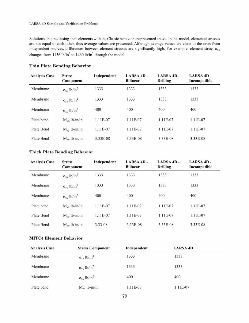
LARSA 4D Sample and Verification Problems
Solutions obtained using shell elements with the Classic behavior are presented above. In this model, elemental stressesare not equal to each other, thus average values are presented. Although average values are close to the ones fromindependent sources, differences between element stresses are significantly high. For example, element stress σxx
changes from 1156 lb/in2 to 1460 lb/in2 through the model.
Thin Plate Bending Behavior
Analysis Case StressComponent
Independent LARSA 4D -Bilinear
LARSA 4D -Drilling
LARSA 4D -Incompatible
Membrane σxx lb/in2 1333 1333 1333 1333
Membrane σyy lb/in2 1333 1333 1333 1333
Membrane σxy lb/in2 400 400 400 400
Plate bend Mxx lb-in/in 1.11E-07 1.11E-07 1.11E-07 1.11E-07
Plate Bend Myy lb-in/in 1.11E-07 1.11E-07 1.11E-07 1.11E-07
Plate Bend Mxy lb-in/in 3.33E-08 3.33E-08 3.33E-08 3.33E-08
Thick Plate Bending Behavior
Analysis Case StressComponent
Independent LARSA 4D -Bilinear
LARSA 4D -Drilling
LARSA 4D -Incompatible
Membrane σxx lb/in2 1333 1333 1333 1333
Membrane σyy lb/in2 1333 1333 1333 1333
Membrane σxy lb/in2 400 400 400 400
Plate bend Mxx lb-in/in 1.11E-07 1.11E-07 1.11E-07 1.11E-07
Plate Bend Myy lb-in/in 1.11E-07 1.11E-07 1.11E-07 1.11E-07
Plate Bend Mxy lb-in/in 3.33-08 3.33E-08 3.33E-08 3.33E-08
MITC4 Element Behavior
Analysis Case Stress Component Independent LARSA 4D
Membrane σxx lb/in2 1333 1333
Membrane σyy lb/in2 1333 1333
Membrane σxy lb/in2 400 400
Plate bend Mxx lb-in/in 1.11E-07 1.11E-07
79

LARSA 4D Sample and Verification Problems
Analysis Case Stress Component Independent LARSA 4D
Plate Bend Myy lb-in/in 1.11E-07 1.11E-07
Plate Bend Mxy lb-in/in 3.33-08 3.33E-08
Contrary to results from the Classic behavior, solutions obtained from the Thin and Thick Plate with Bilinear,Incompatible, and Drilling membrane types and from the MITC4 element behavior compare exactly to the independentsolutions. In addition, stresses and moments are uniform through the entire model.
References• MacNeal, R.H. and Harder, R.L., "A Proposed Standard Set of Problems to Test Finite Element Accuracy,"
Finite Elements Analysis and Design 1 (1985)
• Timoshenko and Goodier, "Theory of Elasticity," 1951, pp. 6.
• Timoshenko and Woinowsky-Krieger, "Theory of plates and shells," 1959, pp. 81.
• SAP 2000, CSI Software Verification Example 2-001, "Shell-Patch test With Prescribed Displacements."
For More Information, please refer to the following documentation.
• For help on linear static analysis, see Linear Static Analysis in LARSA 4D Reference Manual.
80

LARSA 4D Sample and Verification Problems
L22: Shell-Patch Test Using ThermalLoading
This is a patch test for plates suggested by MacNeal and Harder (1985). The model is a rectangular plate with a mesh ofirregularly shaped elements. The plate is subjected to a uniform temperature gradient of +100°F constant through thethickness. The geometry and properties of the plate are equal to those described in problem L21. Joint displacementsand stresses resulting from the temperature load are compared with theoretical solution reported by MacNeal andHarder.
Example Project: The example described here can be found in the Linear Elastic Static folder ofyour LARSA 4D Samples directory (generally My Documents\LARSA Projects\Samples) in the fileL22_Restrained_Thin_Incompatible.
Problem DescriptionTwo different models are created for this example. The models are alike, except for the joint restraints. The first model(namely free expansion) is restrained about all degrees of freedom at joint 1, thus allowing free expansion of the plate.For this model, joint 2 is restrained in Ux direction and joint 7 is restrained in Uy direction for stability conditions.Second model (namely restrained) is pinned at the four corner joints (Joints 1, 2, 7 and 8) and is not free to expandresulting in a stress increase in the elements.
The sign convention for the axes, joint and element labels, joint coordinates, material properties, loading and boundaryconditions are specified in the following figure.
Model diagram
The example model is also created via triangular plates such that each quadrilateral element is divided into twotraingular elements so joint IDs are not changed.
81
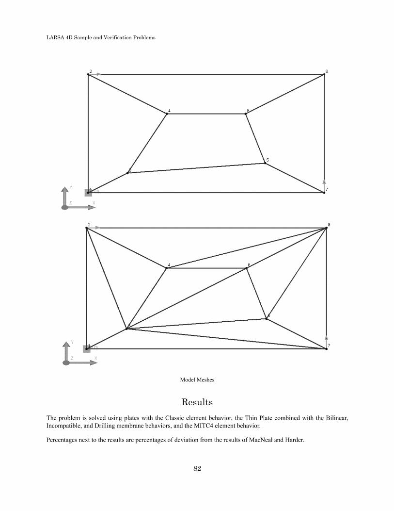
LARSA 4D Sample and Verification Problems
Model Meshes
ResultsThe problem is solved using plates with the Classic element behavior, the Thin Plate combined with the Bilinear,Incompatible, and Drilling membrane behaviors, and the MITC4 element behavior.
Percentages next to the results are percentages of deviation from the results of MacNeal and Harder.
82

LARSA 4D Sample and Verification Problems
Rectangular Plates with Thin Plate Bending Behavior
Model Result MacNeal andHarder
LARSA 4DBilinear
LARSA 4DIncompatible
LARSA 4DDrilling
Free expansion Ux @ joint 8 (in) 0.000132 0.000132 (0%) 0.000132 (0%) 0.000132 (0%)
Free expansion Uy @ joint 8 (in) 0.000066 0.000066 (0%) 0.000066 (0%) 0.000066 (0%)
Free expansion σxx @ joint 8(lb/in2)
0 0 (0%) 0 (0%) 0 (0%)
Free expansion σyy @ joint 8(lb/in2)
0 0 (0%) 0 (0%) 0 (0%)
Restrained Ux @ joint 8 (in) 0 0 (0%) 0 (0%) 0 (0%)
Restrained Uy @ joint 8 (in) 0 0 (0%) 0 (0%) 0 (0%)
Restrained σxx @ joint 8(lb/in2)
-733.33 -733.33 (0%) -733.33 (0%) -733.33 (0%)
Restrained σyy @ joint 8(lb/in2)
-733.33 -733.33 (0%) -733.33 (0%) -733.33 (0%)
Triangular Plates with Thin Plate Bending Behavior and Bilinear Membrane Behavior
Model Result MacNeal and Harder LARSA 4D
Free expansion Ux @ joint 8 (in) 0.000132 0.000132 (0%)
Free expansion Uy @ joint 8 (in) 0.000066 0.000066 (0%)
Free expansion σxx @ joint 8 (lb/in2) 0 0 (0%)
Free expansion σyy @ joint 8 (lb/in2) 0 0 (0%)
Restrained Ux @ joint 8 (in) 0 0 (0%)
Restrained Uy @ joint 8 (in) 0 0 (0%)
Restrained σxx @ joint 8 (lb/in2) -733.33 -733.33 (0%)
Restrained σyy @ joint 8 (lb/in2) -733.33 -733.33 (0%)
MITC4 Element Behavior
Model Result MacNeal and Harder LARSA 4D
Free expansion Ux @ joint 8 (in) 0.000132 0.000132 (0%)
83

LARSA 4D Sample and Verification Problems
Model Result MacNeal and Harder LARSA 4D
Free expansion Uy @ joint 8 (in) 0.000066 0.000066 (0%)
Free expansion σxx @ joint 8 (lb/in2) 0 0 (0%)
Free expansion σyy @ joint 8 (lb/in2) 0 0 (0%)
Restrained Ux @ joint 8 (in) 0 0 (0%)
Restrained Uy @ joint 8 (in) 0 0 (0%)
Restrained σxx @ joint 8 (lb/in2) -733.33 -733.33 (0%)
Restrained σyy @ joint 8 (lb/in2) -733.33 -733.33 (0%)
References• MacNeal, R.H. and Harder, R.L., "A Proposed Standard Set of Problems to Test Finite Element Accuracy,"
Finite Elements Analysis and Design 1 (1985), pp. 3-20, North-Holland.
For More Information, please refer to the following documentation.
• For help on linear static analysis, see Linear Static Analysis in LARSA 4D Reference Manual.
84

LARSA 4D Sample and Verification Problems
L23: Shell-Plate on ElasticFoundation
An isolated 50 kip point load is acting on a one inch thick infinitely large plate that is support on a elastic foundation.Here, the infinitely large plate is modeled as 300 inches long by 300 inches wide and meshed 50 x 50 with a point loadapplied at the center of the plate. The plate deflection at the point load location is compared with independent handcalculated results that are computed using theory presented in Timoshenko and Woinowsky-Krieger 1959.
Problem DescriptionTwo different models are created each using a different soil subgrade modulus. Model A uses a subgrade modulus of30 k/ft3 while Model B uses a subgrade modulus of 800 k/ft3. Those values are chosen to represent approximate upperand lower bound sandy soil stiffnesses.
Model Diagrams
Solution ComparisonThe problem is solved using plates with the MITC4 element behavior.
Model; and Modulus Output parameter Theoretical LARSA 4D
A; (k = 300 k/ft3) Uz at center of plate in -0.9205 -0.9122
85

LARSA 4D Sample and Verification Problems
Model; and Modulus Output parameter Theoretical LARSA 4D
B; (k = 800 k/ft3) Uz at center of plate in -0.1782 -0.1707
References• Timoshenko and Woinowsky-Krieger, "Theory of Plates and Shells," 1959, pp. 275, Equation 185.
For More Information, please refer to the following documentation.
• For help on linear static analysis, see Linear Static Analysis in LARSA 4D Reference Manual.
86
LARSA 4D Sample and Verification Problems
L24: Shell-Curved Beam with StaticLoads
In this example a curved cantilever beam, modeled with shell elements, is subjected to unit forces at the tip in the in-plane and out-plane directions, that is, the Y and Z directions, respectively. The in-plane and out-of-plane loads areapplied in the different load cases.
Problem DescriptionThe geometry, properties and loading are as suggested in MacNeal and Harder 1985. The cantilever beam is bent intoa 90 degree arc. The inner radius is 4.12 inches and the outer is 4.32 inces. It is thus 0.2 inches wide and apporximately6.63 inches long at the centerline. In the Y direction the beam is 0.1 inches thick. For modeling in LARSA 4D, thecurved beam is meshed into six elements, each corresponding a 15 degree arch.
87

LARSA 4D Sample and Verification Problems
Model Diagrams
Loading
Load Case Load
IN Fy= +0.5lb at joints 7 and 14
OUT Fz = +0.5 lb at joint 7 and 14
Solution ComparisonThe problem is solved using plates with the Thin and Thick Plate combined with the Bilinear, Incompatible, andDrilling membrane behaviors, and the MITC4 element behavior.
88

LARSA 4D Sample and Verification Problems
Thin Plate Bending Behavior
Mesh Size Load Case Result Theoretical LARSA 4DDrilling
LARSA 4DBilinear
LARSA 4DIncompatible
SAP2000
6x1 IN Uy avg.ofjnts 7 and14
0.0886 0.0751 0.0064 0.0776 0.0773
90X1 IN Uy avg.ofjnts 91 and182
0.0886 0.0841 0.0789 0.0885 0.0845
90x3 IN Uy avg.ofjnts 91 and182
0.0886 0.0882 0.0833 0.0884 0.0884
6x1 OUT Uz avg.ofjnts 7 and14
0.5004 0.4535 0.4535 0.4535 0.4535
90x1 OUT Uz avg.ofjnts 91 and182
0.5004 0.4512 0.4512 0.4512 0.4514
90x3 OUT Uz avg.ofjnts 91 and182
0.5004 0.4508 0.4508 0.4508 0.4510
For the out of plane load case, the deviation from the theoretical result is due to the shell theory used by LARSA 4Dand the beam theory used for the theoretical solution.
Thick Plate Bending Behavior
Mesh Size Load Case Result Theoretical LARSA 4DDrilling
LARSA 4DBilinear
LARSA 4DIncompatible
SAP2000
6x1 IN Uy avg.ofjnts 7 and14
0.0886 0.0751 0.0064 0.0776 0.0773
90X1 IN Uy avg.ofjnts 91 and182
0.0886 0.0841 0.0789 0.0885 0.0845
90x3 IN Uy avg.ofjnts 91 and182
0.0886 0.0882 0.0833 0.0884 0.0884
6x1 OUT Uz avg.ofjnts 7 and14
0.5004 1.3140 1.3140 1.3140 0.4298
89

LARSA 4D Sample and Verification Problems
Mesh Size Load Case Result Theoretical LARSA 4DDrilling
LARSA 4DBilinear
LARSA 4DIncompatible
SAP2000
90x1 OUT Uz avg.ofjnts 91 and182
0.5004 0.4898 0.4898 0.4898 0.4566
90x3 OUT Uz avg.ofjnts 91 and182
0.5004 0.4964 0.4964 0.4964 0.4558
MITC4 Element Behavior
Mesh Size Load Case Result Theoretical LARSA 4D
6x1 IN Uy avg.of jnts 7 and14
0.0886 0.00641
90X1 IN Uy avg.of jnts 91and 182
0.0886 0.0790
90x3 IN Uy avg.of jnts 91and 182
0.0886 0.0834
6x1 OUT Uz avg.of jnts 7 and14
0.5004 0.4398
90x1 OUT Uz avg.of jnts 91and 182
0.5004 0.6748
90x3 OUT Uz avg.of jnts 91and 182
0.5004 0.4836
Results of LARSA 4D are acceptable comparing to theoretical results, if the mesh size is sufficient.
Increased mesh size reduces distortion from the curved geometry and improves the results.
References• Cook and Young, "Advanced Mechanics of Materials," 1985, pp. 244.
• SAP 2000, CSI Software Verification Example 2-003, "Shell-Curved Beam with Static Loads."
For More Information, please refer to the following documentation.
• For help on linear static analysis, see Linear Static Analysis in LARSA 4D Reference Manual.
90
LARSA 4D Sample and Verification Problems
L25: Shell-Rectangular Plate withStatic Loads
A rectangular plane, modeled with shell elements, is subjected to an out-of-plane point concentrated load, and an out-of-plane uniform load, which is the Z direction. The point concentrated and uniform loads are applied in different states.
Problem DescriptionThe geometry, properties and loading for this problem are based on the publication by MacNeal and Harder 1985. Theplate is 2 inches wide and modeled with both a 2 inch and 10 inch length. Modeled is a quarter plate, consideringboth a 4X4 and 16X16 mesh.
Active in the model are the degrees of freedom for the Z translational, along with the X and Y rotational displacements.In the 4X4 mesh, model symmetry situations are imposed by restraining the X rotational freedom at joints 22, 23, and24; restraining the Y rotational freedom at joints 10, 15, and 20; and restraining both the X and Y rotational freedomat joint 25. The symmetry restraints used in the 16X16 mesh are similar the restraints used above in the 4X4 mesh.Since only a quarter of the plate is modeled, only a quarter of the specified concentrated load is applied to the centerof the plate at joint 25.
Geometry, Properties, and Loading
91

LARSA 4D Sample and Verification Problems
Model Diagram
Solution Comparison2"x2" Think Plate (Uz [in] center of plate)
Mesh Edge Support Load Theoretical LARSA 4D SAP2000
4X4 Simple Uniform -4.06 -4.16 -4.06
16X16 Simple Uniform -4.06 -4.07 -4.06
4X4 Fixed Uniform -1.26 -1.32 -1.32
16X16 Fixed Uniform -1.26 -1.27 -1.27
4X4 Simple Point -11.60 -11.94 -11.94
16X16 Simple Point -11.60 -11.63 -11.63
4X4 Fixed Point -5.60 -5.90 -5.90
16X16 Fixed Point -5.60 -5.64 -5.64
2"x2" Thick Plate (Uz [in] center of plate)
92

LARSA 4D Sample and Verification Problems
Mesh Edge Support Load Theoretical LARSA 4D SAP2000
4X4 Simple Uniform -4.06 -4.33 -4.03
16X16 Simple Uniform -4.06 -4.10 -4.06
4X4 Fixed Uniform -1.26 -1.34 -1.25
16X16 Fixed Uniform -1.26 -1.27 -1.27
4X4 Simple Point -11.60 -12.42 -11.61
16X16 Simple Point -11.60 -11.71 -11.61
4X4 Fixed Point -5.60 -6.08 -5.38
16X16 Fixed Point -5.60 -5.65 -5.61
2"x10" Thin Plate (Uz [in] center of plate)
Mesh Edge Support Load Theoretical LARSA 4D SAP2000
4X4 Simple Uniform -12.97 -12.95 -12.86
16X16 Simple Uniform -12.97 -12.97 -12.96
4X4 Fixed Uniform -2.60 -2.60 -2.60
16X16 Fixed Uniform -2.60 -2.60 -2.60
4X4 Simple Point -16.95 -18.29 -18.12
16X16 Simple Point -16.95 -17.15 -17.15
4X4 Fixed Point -7.25 -7.79 -7.79
16X16 Fixed Point -7.25 -7.41 -7.41
2"x10" Thick Plate (Uz [in] center of plate)
Mesh Edge Support Load Theoretical LARSA 4D SAP2000
4X4 Simple Uniform -12.97 -12.87 -12.87
16X16 Simple Uniform -12.97 -12.99 -12.97
4X4 Fixed Uniform -2.60 -2.60 -2.59
16X16 Fixed Uniform -2.60 -2.60 -2.60
4X4 Simple Point -16.95 -20.83 -16.27
16X16 Simple Point -16.95 -17.53 -16.92
4X4 Fixed Point -7.25 -8.49 -5.86
93

LARSA 4D Sample and Verification Problems
Mesh Edge Support Load Theoretical LARSA 4D SAP2000
16X16 Fixed Point -7.25 -7.52 -7.11
2"x2" MITC4 Plate (Uz [in] center of plate)
Mesh Edge Support Load Theoretical LARSA 4D
4X4 Simple Uniform -4.06 -4.04
16X16 Simple Uniform -4.06 -4.05
4X4 Fixed Uniform -1.26 -1.25
16X16 Fixed Uniform -1.26 -1.26
4X4 Simple Point -11.60 -11.52
16X16 Simple Point -11.60 -11.58
4X4 Fixed Point -5.60 -5.40
16X16 Fixed Point -5.60 -5.60
2"x10" MITC4 Plate (Uz [in] center of plate)
Mesh Edge Support Load Theoretical LARSA 4D
4X4 Simple Uniform -12.97 -12.66
16X16 Simple Uniform -12.97 -12.93
4X4 Fixed Uniform -2.60 -2.48
16X16 Fixed Uniform -2.60 -2.59
4X4 Simple Point -16.95 -15.71
16X16 Simple Point -16.95 -16.82
4X4 Fixed Point -7.25 -5.97
16X16 Fixed Point -7.25 -7.12
References• MacNeal, R.H., Harder, R.L.; "A Proposed Standard Set of Problems to Test Finite Element Accuracy",
Finite Elements in Analysis and Design 1 (1985) 3-20, North-Holand.
• SAP 2000, CSI Software Verification Example 2-005, "Shell-Rectangular Plate with Static Loads"
94

LARSA 4D Sample and Verification Problems
For More Information, please refer to the following documentation.
• For help on linear static analysis, see Linear Static Analysis in LARSA 4D Reference Manual.
95

LARSA 4D Sample and Verification Problems
96

LARSA 4D Sample and Verification Problems
L26: Shell-Scordelis-Lo Roof withStatic Loads
A single span cylindrical barrel vault roof is analyzed for gravity loads. First, the vertical deflection at the center ofthe free edge, displacement and bending moment results along the support and along the central section are computedand compared with published results from MacNeal and Harder 1985. The geometry, properties and loading are alsobased on this publication. Then, twisting moments at support section, transverse and longitudinal moments in centralsection are are computed and compared with published results from Zienkiewicz 1977.
Example Project: The example described here can be found in the LinearStatic folder of your LARSA 4D Samplesdirectory (generally My Documents\LARSA Projects\Samples) in the file L26.
Problem DescriptionThe 3 inch thick roof spans longitudinally 50 feet between supports and is simply supported (Ux and Uy restrained) atits curved ends and is free along the straight edges. The roof has a 25 foot radius and a central angle of 40o. Only aquarter of the roof is modeled to take advantage of symmetry.
A 6 x 6 mesh is used for the quarter roof. In order to impose symmetry conditions, Uz and Rx degrees of freedom ofjoints 44 through 49; Ux and Rz degrees of freedom of joints 1, 8, 15, 22, 29 and 36; Ux, Uz, Rx and Rz degrees offreedom of joint 43 are restrained.
Model Diagrams
LoadingThe loading for this problem is a 90 psf gravity load and is, in other words, a uniform load on the surface area in the -Y direction of 90 psf. Two different load cases are used in order to test two different types of loadings. First the gravityload is applied as self weight then it is applied as a uniform load. In order for the self weight and gravity loads to be90 psf, the unit weight of the concrete is set to 360 lb/ft3.
Load Case Load Type
SELF Self Weight
UNIF Uniform Load
Solution Comparison
Axial Deformation At Support
Here, axial displacements at support joints (joints 1, 2, 3, 4, 5, 6, 7) are computed and results are compared to solutionsfrom the independent source. The model is analyzed using classical bending and classical membrane types, the thick
97

LARSA 4D Sample and Verification Problems
bending type and the thin bending type. For thick and thin bending types, bilinear, drilling and incompatible membranetypes are used.
The following table presents the results from LARSA 4D and from MacNeal and Harder 1985 that are used as anindependent source for comparison. Both load cases give exactly the same results as expected, thus only one table isprovided for both of them.
Axial Deformations at Support
Uz1 (ft) Uz2 (ft) Uz3 (ft) Uz4 (ft) Uz5 (ft) Uz6 (ft) Uz7 (ft)
Independent 4.00E-04 1.00E-03 2.10E-03 3.00E-03 2.10E-03 -2.50E-03 -1.25E-02
Thick -Bilinear
4.70E-05 5.19E-04 1.66E-03 2.67E-03 2.19E-03 -1.58E-03 -1.10E-02
Thick -Drilling
6.00E-05 5.65E-04 1.79E-03 2.85E-03 2.34E-03 -1.69E-03 -1.18E-02
Thick -Incompatible
5.11E-05 5.58E-04 1.78E-03 2.86E-03 2.35E-03 -1.69E-03 -1.18E-02
Thin -Bilinear
4.37E-05 5.17E-04 1.66E-03 2.67E-03 2.20E-03 -1.58E-03 -1.10E-02
Thin-Drilling
5.08E-05 5.58E-04 1.79E-03 2.86E-03 2.36E-03 -1.69E-03 -1.18E-02
Thin -Incompatible
5.52E-05 5.61E-04 1.79E-03 2.86E-03 2.35E-03 -1.69E-03 -1.18E-02
Classical -Classical
3.11E-05 5.43E-04 1.78E-03 2.88E-03 2.38E-03 -1.68E-03 -1.18E-02
The following table presents the deviation of LARSA 4D results from the independent source. The percent differencesare computed using the maximum independent value, 0.0125.
Percent Differences Between LARSA 4D Results and the Independent Source: Axial Deformations at Support
Uz1 Uz2 Uz3 Uz4 Uz5 Uz6 Uz7
Thick -Bilinear
-2.8% -3.8% -3.5% -2.7% 0.7% 7.4% 12.2%
Thick -Drilling
-2.7% -3.5% -2.5% -1.2% 1.9% 6.4% 5.9%
Thick -Incompatible
-2.8% -3.5% -2.5% -1.1% 2.0% 6.5% 5.7%
Thin -Bilinear
-2.9% -3.9% -3.5% -2.7% 0.8% 7.4% 12.2%
98
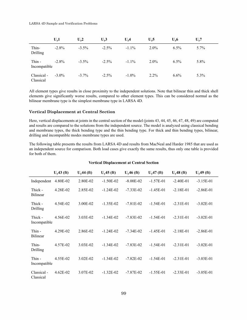
LARSA 4D Sample and Verification Problems
Uz1 Uz2 Uz3 Uz4 Uz5 Uz6 Uz7
Thin-Drilling
-2.8% -3.5% -2.5% -1.1% 2.0% 6.5% 5.7%
Thin -Incompatible
-2.8% -3.5% -2.5% -1.1% 2.0% 6.5% 5.8%
Classical -Classical
-3.0% -3.7% -2.5% -1.0% 2.2% 6.6% 5.3%
All element types give results in close proximity to the independent solutions. Note that bilinear thin and thick shellelements give significantly worse results, compared to other element types. This can be considered normal as thebilinear membrane type is the simplest membrane type in LARSA 4D.
Vertical Displacement at Central Section
Here, vertical displacements at joints in the central section of the model (joints 43, 44, 45, 46, 47, 48, 49) are computedand results are compared to the solutions from the independent source. The model is analyzed using classical bendingand membrane types, the thick bending type and the thin bending type. For thick and thin bending types, bilinear,drilling and incompatible modes membrane types are used.
The following table presents the results from LARSA 4D and results from MacNeal and Harder 1985 that are used asan independent source for comparison. Both load cases give exactly the same results, thus only one table is providedfor both of them.
Vertical Displacement at Central Section
Uy43 (ft) Uy44 (ft) Uy45 (ft) Uy46 (ft) Uy47 (ft) Uy48 (ft) Uy49 (ft)
Independent 4.80E-02 2.80E-02 -1.50E-02 -8.00E-02 -1.57E-01 -2.40E-01 -3.15E-01
Thick -Bilinear
4.28E-02 2.85E-02 -1.24E-02 -7.33E-02 -1.45E-01 -2.18E-01 -2.86E-01
Thick -Drilling
4.54E-02 3.00E-02 -1.35E-02 -7.81E-02 -1.54E-01 -2.31E-01 -3.02E-01
Thick -Incompatible
4.56E-02 3.03E-02 -1.34E-02 -7.83E-02 -1.54E-01 -2.31E-01 -3.02E-01
Thin -Bilinear
4.29E-02 2.86E-02 -1.24E-02 -7.34E-02 -1.45E-01 -2.18E-01 -2.86E-01
Thin-Drilling
4.57E-02 3.03E-02 -1.34E-02 -7.83E-02 -1.54E-01 -2.31E-01 -3.02E-01
Thin -Incompatible
4.55E-02 3.02E-02 -1.34E-02 -7.82E-02 -1.54E-01 -2.31E-01 -3.03E-01
Classical -Classical
4.62E-02 3.07E-02 -1.32E-02 -7.87E-02 -1.55E-01 -2.33E-01 -3.05E-01
99

LARSA 4D Sample and Verification Problems
The following table presents the deviation of LARSA 4D results from the independent source. The percent differencesare computed using the maximum independent value, 0.315.
Percent Differences Between LARSA 4D Results and theIndependent Source: Vertical Displacement at Central Section
Uy43 Uy44 Uy45 Uy46 Uy47 Uy48 Uy49
Thick -Bilinear
-1.6% 0.1% 0.8% 2.1% 3.8% 6.9% 9.1%
Thick -Drilling
-0.8% 0.6% 0.5% 0.6% 1.0% 3.0% 4.1%
Thick -Incompatible
-0.7% 0.7% 0.5% 0.5% 0.9% 2.8% 4.0%
Thin -Bilinear
-1.6% 0.2% 0.8% 2.1% 3.7% 6.9% 9.2%
Thin-Drilling
-0.7% 0.7% 0.5% 0.5% 0.8% 2.8% 4.0%
Thin -Incompatible
-0.8% 0.7% 0.5% 0.6% 0.9% 2.8% 3.9%
Classical -Classical
-0.6% 0.9% 0.6% 0.4% 0.5% 2.2% 3.3%
All element types give results in close proximity to the independent solutions. Note that bilinear thin and thick shellelements give significantly worse results compared to other element types. This can be considered normal as the bilinearmembrane type is the simplest membrane type in LARSA 4D.
Twisting Moments at Support
Here, twisting moments at joints at support section of the model (joints 1, 2, 3, 4, 5, 6, 7) are computed and comparedto the solutions from the independent source. The model is analyzed using classical bending and membrane types,the thick bending type and the thin bending type. For thick and thin bending types, bilinear, drilling and incompatiblemodes membrane types are used.
The following table presents the results from LARSA 4D and results from Zienkiewicz 1977 that are used as anindependent source for comparison. Note that some results had to be interpolated from published graphs. Both loadcases give exactly the same results, thus only one table is provided for both of them.
Twisting Moments at Support
Mxy1 (lb-ft/ft)
Mxy2 (lb-ft/ft)
Mxy3 (lb-ft/ft)
Mxy4 (lb-ft/ft)
Mxy5 (lb-ft/ft)
Mxy6 (lb-ft/ft)
Mxy7 (lb-ft/ft)
Independent 0 -370 -700 -990 -1210 -1310 -1280
Thick -Bilinear
-83 -333 -648 -915 -1247 -1172 -1159
100

LARSA 4D Sample and Verification Problems
Mxy1 (lb-ft/ft)
Mxy2 (lb-ft/ft)
Mxy3 (lb-ft/ft)
Mxy4 (lb-ft/ft)
Mxy5 (lb-ft/ft)
Mxy6 (lb-ft/ft)
Mxy7 (lb-ft/ft)
Thick -Drilling
-90 -358 -695 -980 -1172 -1236 -1223
Thick -Incompatible
-90 -356 -691 -973 -1158 -1216 -1201
Thin -Bilinear
-84 -333 -647 -913 -1091 -1153 -1143
Thin -Drilling
-90 -357 -693 -977 -1167 -1227 -1210
Thin -Incompatible
-89 -356 -692 -976 -1167 -1231 -1219
Classic -Classic
-2 -357 -695 -986 -1181 -1229 -1172
The following table presents the deviation of LARSA 4D results from the independent source. The percent differencesare computed using the maximum independent value, 1310.
Percent Differences Between LARSA 4D Results and the Independent Source: Twisting Moments at Support
Mxy1 Mxy2 Mxy3 Mxy4 Mxy5 Mxy6 Mxy7
Thick -Bilinear
6.3% -2.8% -4.0% -5.7% 2.8% -10.5% -9.2%
Thick -Drilling
6.9% -0.9% -0.4% -0.8% -2.9% -5.6% -4.4%
Thick -Incompatible
6.9% -1.1% -0.7% -1.3% -4.0% -7.2% -6.0%
Thin -Bilinear
6.4% -2.8% -4.0% -5.9% -9.1% -12.0% -10.5%
Thin -Drilling
6.9% -1.0% -0.5% -1.0% -3.3% -6.4% -5.3%
Thin -Incompatible
6.8% -1.0% -0.6% -1.0% -3.3% -6.0% -4.7%
Classic -Classic
0.1% -1.0% -0.4% -0.3% -2.2% -6.2% -8.2%
All element types give results in close proximity to the independent solutions, considering results from the independentsource have to interpolated for some of the joints. Note that bilinear thin and thick shell elements give significantlyworse results compared to other element types. This can be considered normal as the bilinear membrane type is thesimplest membrane type in LARSA 4D.
101
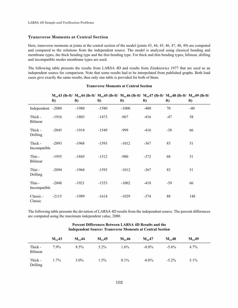
LARSA 4D Sample and Verification Problems
Transverse Moments at Central Section
Here, transverse moments at joints at the central section of the model (joints 43, 44, 45, 46, 47, 48, 49) are computedand compared to the solutions from the independent source. The model is analyzed using classical bending andmembrane types, the thick bending type and the thin bending type. For thick and thin bending types, bilinear, drillingand incompatible modes membrane types are used.
The following table presents the results from LARSA 4D and results from Zienkiewicz 1977 that are used as anindependent source for comparison. Note that some results had to be interpolated from published graphs. Both loadcases give exactly the same results, thus only one table is provided for both of them.
Transverse Moments at Central Section
Mxx43 (lb-ft/ft)
Mxx44 (lb-ft/ft)
Mxx45 (lb-ft/ft)
Mxx46 (lb-ft/ft)
Mxx47 (lb-ft/ft)
Mxx48 (lb-ft/ft)
Mxx49 (lb-ft/ft)
Independent -2080 -1980 -1580 -1000 -400 70 -40
Thick -Bilinear
-1916 -1803 -1473 -967 -416 -47 58
Thick -Drilling
-2045 -1918 -1549 -999 -416 -38 66
Thick -Incompatible
-2093 -1968 -1593 -1012 -367 83 51
Thin -Bilinear
-1955 -1845 -1512 -980 -372 68 51
Thin -Drilling
-2094 -1968 -1593 -1012 -367 83 51
Thin -Incompatible
-2048 -1921 -1553 -1002 -418 -39 66
Classic -Classic
-2115 -1989 -1614 -1029 -374 88 148
The following table presents the deviation of LARSA 4D results from the independent source. The percent differencesare computed using the maximum independent value, 2080.
Percent Differences Between LARSA 4D Results and theIndependent Source: Transverse Moments at Central Section
Mxx43 Mxx44 Mxx45 Mxx46 Mxx47 Mxx48 Mxx49
Thick -Bilinear
7.9% 8.5% 5.2% 1.6% -0.8% -5.6% 4.7%
Thick -Drilling
1.7% 3.0% 1.5% 0.1% -0.8% -5.2% 5.1%
102
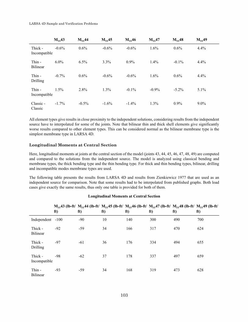
LARSA 4D Sample and Verification Problems
Mxx43 Mxx44 Mxx45 Mxx46 Mxx47 Mxx48 Mxx49
Thick -Incompatible
-0.6% 0.6% -0.6% -0.6% 1.6% 0.6% 4.4%
Thin -Bilinear
6.0% 6.5% 3.3% 0.9% 1.4% -0.1% 4.4%
Thin -Drilling
-0.7% 0.6% -0.6% -0.6% 1.6% 0.6% 4.4%
Thin -Incompatible
1.5% 2.8% 1.3% -0.1% -0.9% -5.2% 5.1%
Classic -Classic
-1.7% -0.5% -1.6% -1.4% 1.3% 0.9% 9.0%
All element types give results in close proximity to the independent solutions, considering results from the independentsource have to interpolated for some of the joints. Note that bilinear thin and thick shell elements give significantlyworse results compared to other element types. This can be considered normal as the bilinear membrane type is thesimplest membrane type in LARSA 4D.
Longitudinal Moments at Central Section
Here, longitudinal moments at joints at the central section of the model (joints 43, 44, 45, 46, 47, 48, 49) are computedand compared to the solutions from the independent source. The model is analyzed using classical bending andmembrane types, the thick bending type and the thin bending type. For thick and thin bending types, bilinear, drillingand incompatible modes membrane types are used.
The following table presents the results from LARSA 4D and results from Zienkiewicz 1977 that are used as anindependent source for comparison. Note that some results had to be interpolated from published graphs. Both loadcases give exactly the same results, thus only one table is provided for both of them.
Longitudinal Moments at Central Section
Myy43 (lb-ft/ft)
Myy44 (lb-ft/ft)
Myy45 (lb-ft/ft)
Myy46 (lb-ft/ft)
Myy47 (lb-ft/ft)
Myy48 (lb-ft/ft)
Myy49 (lb-ft/ft)
Independent -100 -90 10 140 300 490 700
Thick -Bilinear
-92 -59 34 166 317 470 624
Thick -Drilling
-97 -61 36 176 334 494 655
Thick -Incompatible
-98 -62 37 178 337 497 659
Thin -Bilinear
-93 -59 34 168 319 473 628
103

LARSA 4D Sample and Verification Problems
Myy43 (lb-ft/ft)
Myy44 (lb-ft/ft)
Myy45 (lb-ft/ft)
Myy46 (lb-ft/ft)
Myy47 (lb-ft/ft)
Myy48 (lb-ft/ft)
Myy49 (lb-ft/ft)
Thin -Drilling
-97 -61 38 178 337 497 658
Thin -Incompatible
-97 -61 36 176 335 495 656
Classic -Classic
-121 -83 21 171 344 518 658
The following table presents the deviation of LARSA 4D results from the independent source. The percent differencesare computed using the maximum independent value, 700.
Percent Differences Between LARSA 4D Results and theIndependent Source: Longitudinal Moments at Central Section
Myy43 Myy44 Myy45 Myy46 Myy47 Myy48 Myy49
Thick -Bilinear
1.2% 4.5% 3.4% 3.7% 2.5% -2.8% -10.9%
Thick -Drilling
0.5% 4.1% 3.8% 5.1% 4.8% 0.6% -6.4%
Thick -Incompatible
0.3% 4.0% 3.8% 5.4% 5.3% 1.0% -5.8%
Thin -Bilinear
1.0% 4.4% 3.4% 4.0% 2.8% -2.5% -10.3%
Thin -Drilling
0.4% 4.1% 3.9% 5.5% 5.3% 1.0% -5.9%
Thin -Incompatible
0.5% 4.1% 3.8% 5.2% 4.9% 0.7% -6.3%
Classic -Classic
-2.9% 1.0% 1.5% 4.5% 6.3% 4.0% -6.0%
All element types give results in close proximity to the independent solutions, considering results from the independentsource have to interpolated for some of the joints. Note that bilinear thin and thick shell elements give significantlyworse results compared to other element types. This can be considered normal as the bilinear membrane type is thesimplest membrane type in LARSA 4D.Sources:
• MacNeal, R.H. and Harder, R.L., "A Proposed Standard Set of Problems to Test Finite Element Accuracy," Finite Elements Analysis and Design 1 (1985).
• SAP 2000, CSI Software Verification Example 2-006, "Shell-Scordelis-Lo Roof with Static Loads."
• Zienkiewicz, "The Finite Element Method" 1977, pp. 350, Figure 13.11c.
104

LARSA 4D Sample and Verification Problems
For More Information, please refer to the following documentation.
• For help on linear static analysis, see Linear Static Analysis in LARSA 4D Reference Manual.
105

LARSA 4D Sample and Verification Problems
106
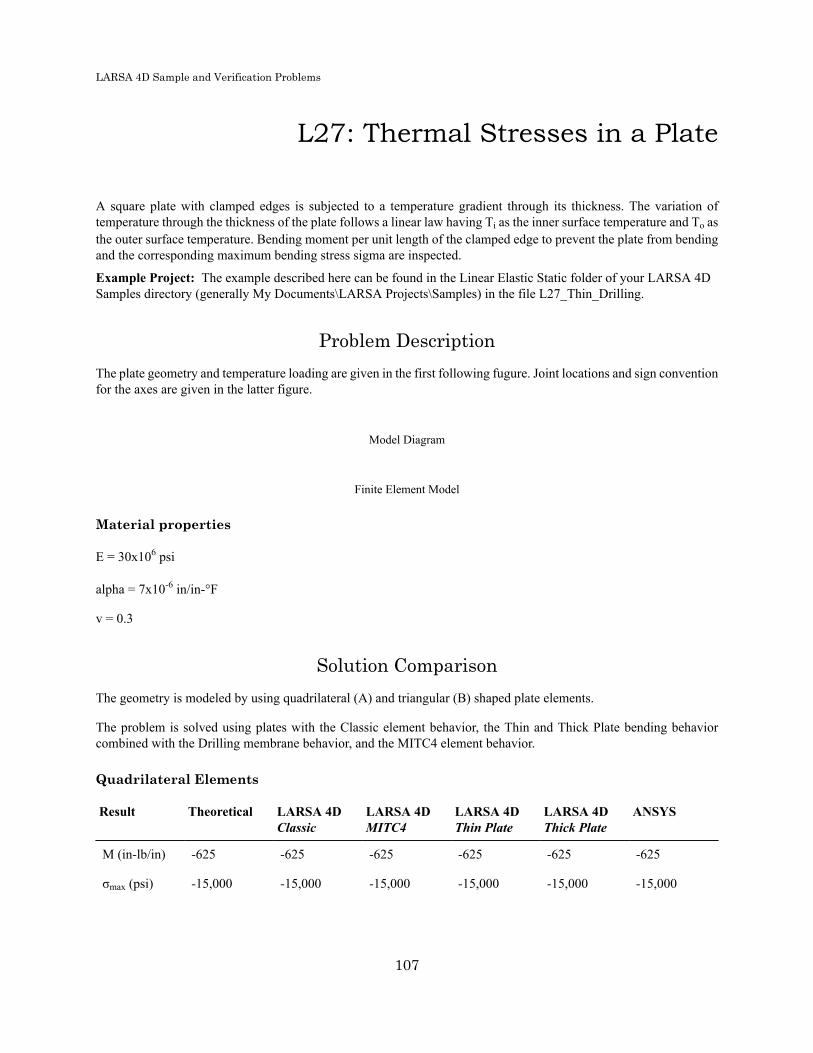
LARSA 4D Sample and Verification Problems
L27: Thermal Stresses in a Plate
A square plate with clamped edges is subjected to a temperature gradient through its thickness. The variation oftemperature through the thickness of the plate follows a linear law having Ti as the inner surface temperature and To asthe outer surface temperature. Bending moment per unit length of the clamped edge to prevent the plate from bendingand the corresponding maximum bending stress sigma are inspected.
Example Project: The example described here can be found in the Linear Elastic Static folder of your LARSA 4DSamples directory (generally My Documents\LARSA Projects\Samples) in the file L27_Thin_Drilling.
Problem DescriptionThe plate geometry and temperature loading are given in the first following fugure. Joint locations and sign conventionfor the axes are given in the latter figure.
Model Diagram
Finite Element Model
Material properties
E = 30x106 psi
alpha = 7x10⁻⁶ in/in-°F
v = 0.3
Solution ComparisonThe geometry is modeled by using quadrilateral (A) and triangular (B) shaped plate elements.
The problem is solved using plates with the Classic element behavior, the Thin and Thick Plate bending behaviorcombined with the Drilling membrane behavior, and the MITC4 element behavior.
Quadrilateral Elements
Result Theoretical LARSA 4DClassic
LARSA 4DMITC4
LARSA 4DThin Plate
LARSA 4DThick Plate
ANSYS
M (in-lb/in) -625 -625 -625 -625 -625 -625
σmax (psi) -15,000 -15,000 -15,000 -15,000 -15,000 -15,000
107

LARSA 4D Sample and Verification Problems
Triangular Elements
Result Theoretical LARSA 4DThin Plate
LARSA 4DThick Plate
ANSYS
M (in-lb/in) -625 -625 -625 -625
σmax (psi) -15,000 -15,000 -15,000 -15,000
References• ANYSYS, Verification Problem No.23, "Thermal Stresses in a Plate."
• Timoshenko, "Strength of Materials" 1956, pp. 91, Equation 87, (ref.4).
For More Information, please refer to the following documentation.
• For help on linear static analysis, see Linear Static Analysis in LARSA 4D Reference Manual.
108

LARSA 4D Sample and Verification Problems
L28: Shell-Temperature GradientThrough Shell Thickness
A flat annular plate is subjected to a linear temperature gradient through its thickness.
Example Project: The example described here can be found in the Linear Elastic Static folder of your LARSA 4DSamples directory (generally My Documents\LARSA Projects\Samples) in the file L28_Thin_Drilling.
Problem DescriptionThe plate has an inner radius of 3 inches and an outer radius of 30 inches. Its thickness is 1 inch. The mesh of thismodel consists of 144 quad-shaped shell elements, which are distributed in a structured manner in which 9 radial and16 angular sections divide the shell elements (Model A). The same model is repeated by using triangular shell elementsalso (Model B). The resulting mesh models are given in following the figure.
Mesh with Quad Shells (A) (left), Mesh with Triangular Shells (B) (right)
The local axes of all shell elements are oriented in such a way that the local x-axis is radial and the local y-axis istangential. The local axes are defined in this manner so that the desired results are constant along the perimeters. Thelocal axis that points to the radial direction is named as 1 and the tangential local axis is named as 2 in the results.
Loading and boundary conditions
The applied temperature gradient is 100 oF per inch with linear variation through plate thickness. The bottom is warmerthan the top of the plate. Linear static analysis is performed with only this load case.
109

LARSA 4D Sample and Verification Problems
The joints at the outer edge are clamped in all degrees of freedom.
Material properties
E = 29,000 ksi
alpha = 6.5x10⁻⁶ in/in-oF
v = 0.3
ResultsDisplacement, rotation and moment results are compared with hand calculations based on formulas presented in Roarkand Young 1975 as well as the results documented in SAP2000's manuals.
The problem is solved using plates with Thin and Thick Plate bending behavior and the MITC4 element behavior.
The percentage difference from independent results are given next to the results in parentheses.
In the LARSA 4D project file for this problem, Uz values are taken from joint 2 Uz displacement; R2 values are takenfrom joint 2 Ry displacement since in this joint, y direction is coinciding with the tangential vector. For Model A,M11 results are taken from plate 145's internal reaction at joint 146 in Mxx direction and multiplied by -1 since M11is outwards and Myy is inwards; M22 results are taken from plate 17's internal reaction at joint 2 in Myy direction andmultiplied by -1 since LARSA 4D's sign convention of plates about moments is the opposite of independent results'sign convention. On the other hand, for Model B, Mxx and Myy results are taken from the internal moment of plate 24at joint 17 and plate 160 at joint 1, respectively.
Quadrilateral Thin Plate
Result Independent LARSA 4D SAP2000
Uz @ inner edge (in) 0.01931 0.01905 (-1%) 0.01905 (-1%)
R2 @ inner edge (rad) 0.00352 0.00347 (-1%) 0.00347 (-1%)
M11 @ outer edge (k-in/in)
-2.18100 -2.18209 (0%) -2.18200 (0%)
M22 @ inner edge (k-in/in)
-4.40600 -4.53398 (3%) -4.01600 (-9%)
Quadrilateral Thick Plate
Result Independent LARSA 4D SAP2000
Uz @ inner edge (in) 0.01931 0.01859 (-4%) 0.01778 (-8%)
R2 @ inner edge (rad) 0.00352 0.00320 (-9%) 0.00311 (-12%)
M11 @ outer edge (k-in/in)
-2.18100 -2.18185 (0%) -2.18500 (0%)
110

LARSA 4D Sample and Verification Problems
Result Independent LARSA 4D SAP2000
M22 @ inner edge (k-in/in)
-4.40600 -4.31723 (-2%) -4.47800 (2%)
Quadrilateral MITC4 Plate
Result Independent LARSA 4D
Uz @ inner edge (in) 0.01931 0.01859 (-4%)
R2 @ inner edge (rad) 0.00352 0.00320 (-9%)
M11 @ outer edge (k-in/in) -2.18100 -2.18188 (0%)
M22 @ inner edge (k-in/in) -4.40600 -4.64490 (5%)
Triangular Thin Plate
Result Independent LARSA 4D SAP2000
Uz @ inner edge (in) 0.01931 0.01616 (-16%) 0.01616 (-16%)
R2 @ inner edge (rad) 0.00352 0.00272 (-23%) 0.00272 (-23%)
M11 @ outer edge (k-in/in)
-2.1810 -2.1932 (1%) -2.1840 (0%)
M22 @ inner edge (k-in/in)
-4.4060 -4.3771 (-1%) -4.3769 (-1%)
Triangular Thick Plate
Result Independent LARSA 4D SAP2000
Uz @ inner edge (in) 0.01931 0.01757 (-9%) 0.01551 (-20%)
R2 @ inner edge (rad) 0.00352 0.00302 (-14%) 0.00258 (-27%)
M11 @ outer edge (k-in/in)
-2.1810 -2.1887 (0%) -2.1911 (0%)
M22 @ inner edge (k-in/in)
-4.4060 -4.6904 (6%) -4.2930 (-3%)
References• Roark and Young, "Roark's Formulas for Stress and Strain," 1975, p.361
• SAP 2000, CSI Software Verification Example 2-014, "Shell-Temperature gradient Through ShellThickness."
111

LARSA 4D Sample and Verification Problems
For More Information, please refer to the following documentation.
• For help on linear static analysis, see Linear Static Analysis in LARSA 4D Reference Manual.
112

LARSA 4D Sample and Verification Problems
L29: Solid-Straight Beam with StaticLoads
A straight cantilever beam, modeled with solid objects, is subjected to unit forces at the tip in the three orthogonaldirections and a unit moment at the tip about the three orthogonal directions, each in a different load case.
Problem DescriptionA straight cantilever beam, modeled with solid objects, is subjected to unit forces at the tip in the three orthogonaldirections and a unit moment at the tip about the three orthogonal directions, each in a different load case.
The basic geometry, properties and loading are as described in the publication by MacNeal and Harder 1985. Thecantilever beam is 6 inches long, 0.2 inch wide parallel to the z direction and 0.1 inch wide parallel to the Y direction.The three different models are created to each represent a different element shape. Models A, B and C use rectangular-,trapazoidal- and parallelogram-shaped elements, respectively.
Please note that this example is an extreme case presented for testing and verification of the solid object. Solid objectsare not in general intended for use in modeling a beam with an nx1x1 mesh.
Of the six load cases created for each model, load cases 1 through 3 apply unit forces at the cantilever tip in the X,Y and Z directions and load cases 4 through 6 apply unit moments at the cantilever tip about X, Y and Z directions,respectively. The moments are applied as couples.
The independent solution is derived using elementary beam theory that assumes no local Poisson's effect occurs at thesupport. The beam is modeled in LARSA 4D with all joints fully restrained at the fixed end and with all joints at thefree end assigned to a body constraint. Thus, the LARSA 4D model is slightly different from the free hand calculationsbecause in the LARSA 4D model there is a slight local Poisson's effect at the beam ends.
Model Diagrams
Data
E = 10,000,000 lb/in2
v = 0.3
G = 3,846,154 lb/in2
Solid object thickness in Y direction = 0.1 in
113

LARSA 4D Sample and Verification Problems
Loading
Load Case Load Type Load
1 Px Axial Extension Fx = +0.25 lb joints 7, 14, 21 and 28
2 Vz and My Shear and bending Fz = +0.25 lb joints 7, 14, 21 and 28
3 Vy and Mz Shear and bending Fy = +0.25 lb joints 7, 14, 21 and 28
4 Mx Twist Fy = -2.5 lb joints 7 and 21 Fy =+2.5 lb joints 14 and 28
5 My Moment Fx = -2.5 lb joints 7 and 21 Fx =+2.5 lb joints 14 and 28
6 Mz Moment Fy = +5 lb joints 7 and 14 Fy = -5 lbjoints 21 and 28
The following tables summarize the results for Models A-C with Incompatible Bending for their Load Case and Type.
Results WITH Incompatible Bending Modes for Load Case 1; Px Axial Entension
Load Case;and Type
Model andElementShape
Mesh OutputParameter
Theoretical LARSA4D SAP2000
Load Case1; Px AxialExtension
A- Rectangle 6X1X1 average ofjoints 7, 14,21, and 28 in
3.000E-05 --- 2.962E-05
Load Case1; Px AxialExtension
A- Rectangle 30X1X1 average ofjoints 7, 14,21, and 28 in
3.000E-05 --- 2.985E-05
Load Case1; Px AxialExtension
A- Rectangle 30X4X8 average ofjoints 77, 14,21, and 28 in
3.000E-05 --- 2.984E-05
Load Case1; Px AxialExtension
B- Trapezoid 6X1X1 average ofjoints 7, 14,21, and 28 in
3.000E-05 --- 2.966E-05
Load Case1; Px AxialExtension
B- trapezoid 30X1X1 average ofjoint 7, 14,21, and 28 in
3.000E-05 --- 2.985E-05
Load Case1; Px AxialExtension
B- Trapezoid 30X4X8 average ofjoints 7, 14,21, and 28 in
0.1081 --- 2.985E-05
114

LARSA 4D Sample and Verification Problems
Load Case;and Type
Model andElementShape
Mesh OutputParameter
Theoretical LARSA4D SAP2000
Load Case1; Px AxialExtension
C-Parellelogram
6X1X1 average ofjoints 77, 14,21, and 28 in
0.1081 --- 2.965E-05
Load Case1; Px AxialExtension
C-Parrellelogram
30X1X1 average ofjoints 7, 14,21, and 28 in
0.1081 --- 2.985E-05
Load Case1; Px AxialExtension
C-Parellelogram
30X4X8 average ofjoints 7, 14,21, and 28 in
0.1081 --- 2.985E-05
Results WITH Incompatible Bending Modes for Load Case 2; Vz and My Shear and bending
Load Case;and Type
Model andElementShape
Mesh OutputParameter
Theoretical LARSA4D SAP2000
Load Case2; Vz and MyShear andBending
A- Rectangle 6X1X1 average ofjoint 7, 14,21, and 28 in
0.1081 --- 0.1057
Load Case2; Vz and MyShear andBending
A- Rectangle 30X1X1 average ofjoint 7, 14,21, and 28 in
0.1081 --- 0.1.077
Load Case2; Vz and MyShear andBending
A- Rectangle 30X4X8 average ofjoint 7, 14,21, and 28 in
0.1081 --- 0.1073
Load Case2; Vz and MyShear andBending
B- Trapezoid 6X1X1 average ofjoint 7, 14,21, and 28 in
0.1081 --- 0.0051
Load Case2; Vz and MyShear andBending
B- Trapezoid 30X1X1 average ofjoint 7, 14,21, and 28 in
0.1081 --- 0.1071
Load Case2; Vz and MyShear andBending
B- Trapezoid 30X4X8 average ofjoint 7, 14,21, and 28 in
0.1081 --- 0.1069
115

LARSA 4D Sample and Verification Problems
Load Case;and Type
Model andElementShape
Mesh OutputParameter
Theoretical LARSA4D SAP2000
Load Case2; Vz and MyShear andBending
C-parellelogram
6X1X1 average ofjoint 7, 14,21, and 28 in
0.1081 --- 0.0673
Load Case2; Vz and MyShear andBending
C-parellelogram
30X1X1 average ofjoint 7, 14,21, and 28 in
0.1081 --- 0.1076
Load Case2; Vz and MyShear andBending
C-parellelogram
30X4X8 average ofjoint 7, 14,21, and 28 in
0.1081 --- 0.1072
Results WITH Incompatible Bending Modes for Load Case 3; Vy and Mz Shear and bending
Load Case;and Type
Model andElementShape
Mesh OutputParameter
Theoretical LARSA4D SAP2000
Load Case3; Vz and MzShear andBending
A- Rectangle 6X1X1 average ofjoint 7, 14,21, and 28 in
0.4321 --- 0.4203
Load Case3; Vz and MzShear andBending
A- Rectangle 30X1X1 average ofjoint 7, 14,21, and 28 in
0.4321 --- 0.4300
Load Case3; Vz and MzShear andBending
A- Rectangle 30X4X8 average ofjoint 7, 14,21, and 28 in
0.4321 --- 0.4286
Load Case3; Vz and MzShear andBending
B- trapezoid 6X1X1 average ofjoint 7, 14,21, and 28 in
0.4321 --- 0.0129
Load Case3; Vz and MzShear andBending
B- trapezoid 30X1X1 average ofjoint 7, 14,21, and 28 in
0.4321 --- 0.4060
Load Case3; Vz and Mz
B- trapezoid 30X4X8 average ofjoint 7, 14,21, and 28 in
0.4321 --- 0.4246
116
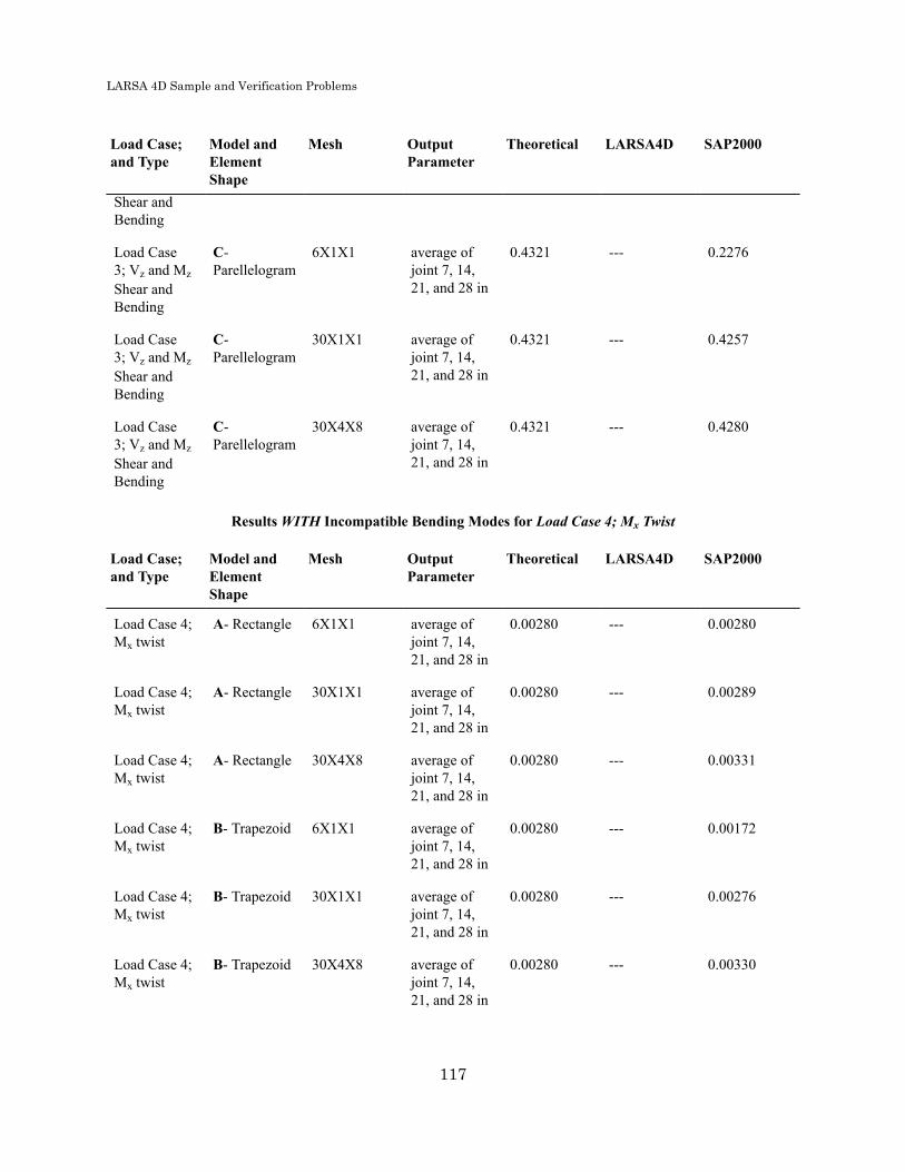
LARSA 4D Sample and Verification Problems
Load Case;and Type
Model andElementShape
Mesh OutputParameter
Theoretical LARSA4D SAP2000
Shear andBending
Load Case3; Vz and MzShear andBending
C-Parellelogram
6X1X1 average ofjoint 7, 14,21, and 28 in
0.4321 --- 0.2276
Load Case3; Vz and MzShear andBending
C-Parellelogram
30X1X1 average ofjoint 7, 14,21, and 28 in
0.4321 --- 0.4257
Load Case3; Vz and MzShear andBending
C-Parellelogram
30X4X8 average ofjoint 7, 14,21, and 28 in
0.4321 --- 0.4280
Results WITH Incompatible Bending Modes for Load Case 4; Mx Twist
Load Case;and Type
Model andElementShape
Mesh OutputParameter
Theoretical LARSA4D SAP2000
Load Case 4;Mx twist
A- Rectangle 6X1X1 average ofjoint 7, 14,21, and 28 in
0.00280 --- 0.00280
Load Case 4;Mx twist
A- Rectangle 30X1X1 average ofjoint 7, 14,21, and 28 in
0.00280 --- 0.00289
Load Case 4;Mx twist
A- Rectangle 30X4X8 average ofjoint 7, 14,21, and 28 in
0.00280 --- 0.00331
Load Case 4;Mx twist
B- Trapezoid 6X1X1 average ofjoint 7, 14,21, and 28 in
0.00280 --- 0.00172
Load Case 4;Mx twist
B- Trapezoid 30X1X1 average ofjoint 7, 14,21, and 28 in
0.00280 --- 0.00276
Load Case 4;Mx twist
B- Trapezoid 30X4X8 average ofjoint 7, 14,21, and 28 in
0.00280 --- 0.00330
117

LARSA 4D Sample and Verification Problems
Load Case;and Type
Model andElementShape
Mesh OutputParameter
Theoretical LARSA4D SAP2000
Load Case 4;Mx twist
C-Parellelogram
6X1X1 average ofjoint 7, 14,21, and 28 in
0.00280 --- 0.00255
Load Case 4;Mx twist
C-Parellelogram
30X1X1 average ofjoint 7, 14,21, and 28 in
0.00280 --- 0.00288
Load Case 4;Mx twist
C-Parellelogram
30X4X8 average ofjoint 7, 14,21, and 28 in
0.00280 --- 0.00331
Results WITH Incompatible Bending Modes for Load Case 5; My Moment
Load Case;and Type
Model andElementShape
Mesh OutputParameter
Theoretical LARSA4D SAP2000
Load Case 5;My Moment
A- Rectangle 6X1X1 average ofjoint 7, 14,21, and 28 in
9.00E-04 --- 8.906E-04
Load Case 5;My Moment
A- Rectangle 30X1X1 average ofjoint 7, 14,21, and 28 in
9.00E-04 --- 8.981E-04
Load Case 5;My Moment
A- Rectangle 30X4X8 average ofjoint 7, 14,21, and 28 in
9.00E-04 --- 8.955E-04
Load Case 5;My Moment
B- Trapezoid 6X1X1 average ofjoint 7, 14,21, and 28 in
9.00E-04 --- 3.240E-05
Load Case 5;My Moment
B- Trapezoid 30X1X1 average ofjoint 7, 14,21, and 28 in
9.00E-04 --- 8.930E-04
Load Case 5;My Moment
B- Trapezoid 30X4X8 average ofjoint 7, 14,21, and 28 in
9.00E-04 --- 8.921E-04
Load Case 5;My Moment
C-Parellelogram
6X1X1 average ofjoint 7, 14,21, and 28 in
9.00E-04 --- 6.369E-04
Load Case 5;My Moment
C-Parellelogram
30X1X1 average ofjoint 7, 14,21, and 28 in
9.00E-04 --- 8.976E-04
118
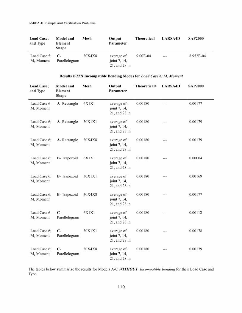
LARSA 4D Sample and Verification Problems
Load Case;and Type
Model andElementShape
Mesh OutputParameter
Theoretical LARSA4D SAP2000
Load Case 5;My Moment
C-Parellelogram
30X4X8 average ofjoint 7, 14,21, and 28 in
9.00E-04 --- 8.952E-04
Results WITH Incompatible Bending Modes for Load Case 6; Mz Moment
Load Case;and Type
Model andElementShape
Mesh OutputParameter
Theoretical> LARSA4D SAP2000
Load Case 6Mz Moment
A- Rectangle 6X1X1 average ofjoint 7, 14,21, and 28 in
0.00180 --- 0.00177
Load Case 6;Mz Moment
A- Rectangle 30X1X1 average ofjoint 7, 14,21, and 28 in
0.00180 --- 0.00179
Load Case 6;Mz Moment
A- Rectangle 30X4X8 average ofjoint 7, 14,21, and 28 in
0.00180 --- 0.00179
Load Case 6;Mz Moment
B- Trapezoid 6X1X1 average ofjoint 7, 14,21, and 28 in
0.00180 --- 0.00004
Load Case 6;Mz Moment
B- Trapezoid 30X1X1 average ofjoint 7, 14,21, and 28 in
0.00180 --- 0.00169
Load Case 6;Mz Moment
B- Trapezoid 30X4X8 average ofjoint 7, 14,21, and 28 in
0.00180 --- 0.00177
Load Case 6Mz Moment
C-Parellelogram
6X1X1 average ofjoint 7, 14,21, and 28 in
0.00180 --- 0.00112
Load Case 6;Mz Moment
C-Parellelogram
30X1X1 average ofjoint 7, 14,21, and 28 in
0.00180 --- 0.00178
Load Case 6;Mz Moment
C-Parellelogram
30X4X8 average ofjoint 7, 14,21, and 28 in
0.00180 --- 0.00179
The tables below summarize the results for Models A-C WITHOUT Incompatible Bending for their Load Case andType.
119

LARSA 4D Sample and Verification Problems
Load Case;and Type
Model andElementShape
Mesh OutputParameter
Theoretical LARSA4D SAP2000
Load Case1; Px AxialExtension
A- Rectangle 6X1X1 average ofjoints 7, 14,21, and 28 in
3.000E-05 --- 2.914E-05
Load Case1; Px AxialExtension
A- Rectangle 30X1X1 average ofjoints 7, 14,21, and 28 in
3.000E-05 --- 2.982E-05
Load Case1; Px AxialExtension
A- Rectangle 30X4X8 average ofjoints 77, 14,21, and 28 in
3.000E-05 --- 2.995E-05
Load Case1; Px AxialExtension
B- Trapezoid 6X1X1 average ofjoints 7, 14,21, and 28 in
3.000E-05 --- 2.915E-05
Load Case1; Px AxialExtension
B- trapezoid 30X1X1 average ofjoint 7, 14,21, and 28 in
3.000E-05 --- 2.982E-05
Load Case1; Px AxialExtension
B- Trapezoid 30X4X8 average ofjoints 7, 14,21, and 28 in
3.000E-05 --- 2.995E-05
Load Case1; Px AxialExtension
C-Parellelogram
6X1X1 average ofjoints 77, 14,21, and 28 in
3.000E-05 --- 2.915E-05
Load Case1; Px AxialExtension
C-Parrellelogram
30X1X1 average ofjoints 7, 14,21, and 28 in
3.000E-05 --- 2.982E-05
Load Case1; Px AxialExtension
C-Parellelogram
30X4X8 average ofjoints 7, 14,21, and 28 in
3.000E-05 --- 2.995E-05
Results WITH Incompatible Bending Modes for Load Case 2; Vz and My Shear and bending
Load Case;and Type
Model andElementShape
Mesh OutputParameter
Theoretical LARSA4D SAP2000
Load Case2; Vz and MyShear andBending
A- Rectangle 6X1X1 average ofjoint 7, 14,21, and 28 in
0.1081 --- 0.0100
120

LARSA 4D Sample and Verification Problems
Load Case;and Type
Model andElementShape
Mesh OutputParameter
Theoretical LARSA4D SAP2000
Load Case2; Vz and MyShear andBending
A- Rectangle 30X1X1 average ofjoint 7, 14,21, and 28 in
0.1081 --- 0.0718
Load Case2; Vz and MyShear andBending
A- Rectangle 30X4X8 average ofjoint 7, 14,21, and 28 in
0.1081 --- 0.1070
Load Case2; Vz and MyShear andBending
B- Trapezoid 6X1X1 average ofjoint 7, 14,21, and 28 in
0.1081 --- 0.0028
Load Case2; Vz and MyShear andBending
B- Trapezoid 30X1X1 average ofjoint 7, 14,21, and 28 in
0.1081 --- 0.0452
Load Case2; Vz and MyShear andBending
B- Trapezoid 30X4X8 average ofjoint 7, 14,21, and 28 in
0.1081 --- 0.1047
Load Case2; Vz and MyShear andBending
C-parellelogram
6X1X1 average ofjoint 7, 14,21, and 28 in
0.1081 --- 0.0034
Load Case2; Vz and MyShear andBending
C-parellelogram
30X1X1 average ofjoint 7, 14,21, and 28 in
0.1081 --- 0.0296
Load Case2; Vz and MyShear andBending
C-parellelogram
30X4X8 average ofjoint 7, 14,21, and 28 in
0.1081 --- 0.1016
Results WITH Incompatible Bending Modes for Load Case 3; Vy and Mz Shear and bending
Load Case;and Type
Model andElementShape
Mesh OutputParameter
Theoretical LARSA4D SAP2000
Load Case3; Vy and Mz
A- Rectangle 6X1X1 average ofjoint 7, 14,21, and 28 in
0.4321 --- 0.0109
121

LARSA 4D Sample and Verification Problems
Load Case;and Type
Model andElementShape
Mesh OutputParameter
Theoretical LARSA4D SAP2000
Shear andBending
Load Case3; Vy and MzShear andBending
A- Rectangle 30X1X1 average ofjoint 7, 14,21, and 28 in
0.4321 --- 0.1558
Load Case3; Vy and MzShear andBending
A- Rectangle 30X4X8 average ofjoint 7, 14,21, and 28 in
0.4321 --- 0.4168
Load Case3; Vy and MzShear andBending
B- trapezoid 6X1X1 average ofjoint 7, 14,21, and 28 in
0.4321 --- 0.0045
Load Case3; Vy and MzShear andBending
B- trapezoid 30X1X1 average ofjoint 7, 14,21, and 28 in
0.4321 --- 0.1345
Load Case3; Vy and MzShear andBending
B- trapezoid 30X4X8 average ofjoint 7, 14,21, and 28 in
0.4321 --- 0.4135
Load Case3; Vy and MzShear andBending
C-Parellelogram
6X1X1 average ofjoint 7, 14,21, and 28 in
0.4321 --- 0.0062
Load Case3; Vy and MzShear andBending
C-Parellelogram
30X1X1 average ofjoint 7, 14,21, and 28 in
0.4321 --- 0.1169
Load Case3; Vy and MzShear andBending
C-Parellelogram
30X4X8 average ofjoint 7, 14,21, and 28 in
0.4321 --- 0.4084
Results WITH Incompatible Bending Modes for Load Case 4; Mx Twist
122

LARSA 4D Sample and Verification Problems
Load Case;and Type
Model andElementShape
Mesh OutputParameter
Theoretical LARSA4D SAP2000
Load Case 4;Mx Twist
A- Rectangle 6X1X1 average ofjoint 7, 14,21, and 28 in
0.00341 --- 0.00280
Load Case 4;Mx Twist
A- Rectangle 30X1X1 average ofjoint 7, 14,21, and 28 in
0.00341 --- 0.00289
Load Case 4;Mx Twist
A- Rectangle 30X4X8 average ofjoint 7, 14,21, and 28 in
0.00341 --- 0.00331
Load Case 4;Mx Twist
B- Trapezoid 6X1X1 average ofjoint 7, 14,21, and 28 in
0.00341 --- 0.00159
Load Case 4;Mx Twist
B- Trapezoid 30X1X1 average ofjoint 7, 14,21, and 28 in
0.00341 --- 0.00183
Load Case 4;Mx Twist
B- Trapezoid 30X4X8 average ofjoint 7, 14,21, and 28 in
0.00341 --- 0.00322
Load Case 4;Mx Twist
C-Parellelogram
6X1X1 average ofjoint 7, 14,21, and 28 in
0.00341 --- 0.00108
Load Case 4;Mx Twist
C-Parellelogram
30X1X1 average ofjoint 7, 14,21, and 28 in
0.00341 --- 0.00320
Load Case 4;Mx Twist
C-Parellelogram
30X4X8 average ofjoint 7, 14,21, and 28 in
0.00341 --- 0.00310
Results WITH Incompatible Bending Modes for Load Case 5; My Moment
Load Case;and Type
Model andElementShape
Mesh OutputParameter
Theoretical LARSA4D SAP2000
Load Case 5;My Moment
A- Rectangle 6X1X1 average ofjoint 7, 14,21, and 28 in
9.00E-04 --- 8.370E-05
Load Case 5;My Moment
A- Rectangle 30X1X1 average ofjoint 7, 14,21, and 28 in
9.00E-04 --- 5.983E-04
123
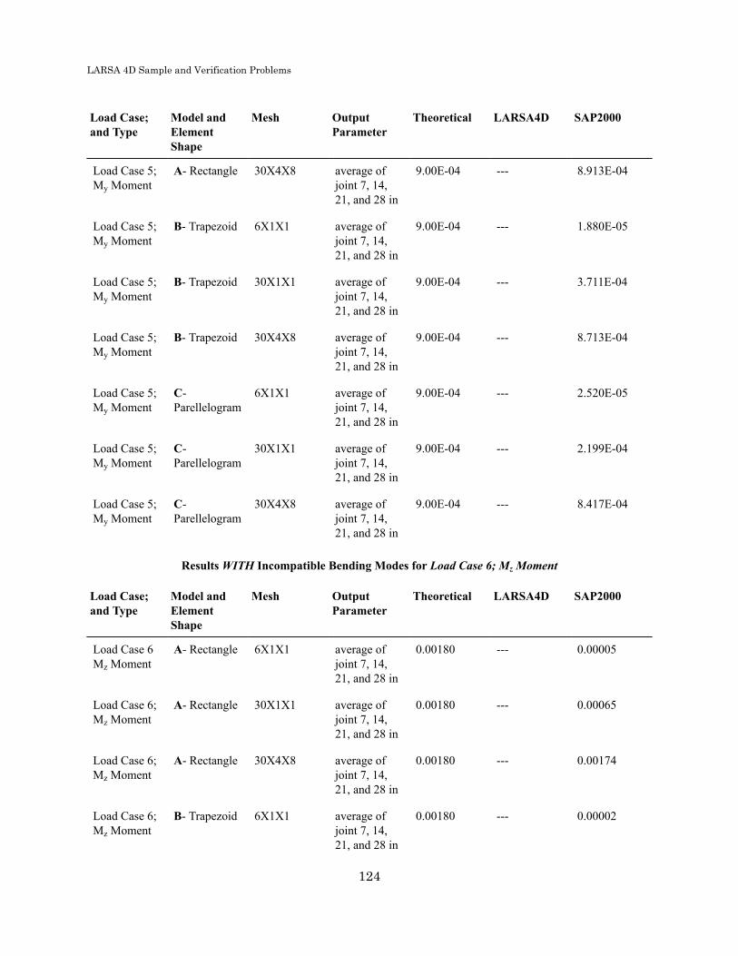
LARSA 4D Sample and Verification Problems
Load Case;and Type
Model andElementShape
Mesh OutputParameter
Theoretical LARSA4D SAP2000
Load Case 5;My Moment
A- Rectangle 30X4X8 average ofjoint 7, 14,21, and 28 in
9.00E-04 --- 8.913E-04
Load Case 5;My Moment
B- Trapezoid 6X1X1 average ofjoint 7, 14,21, and 28 in
9.00E-04 --- 1.880E-05
Load Case 5;My Moment
B- Trapezoid 30X1X1 average ofjoint 7, 14,21, and 28 in
9.00E-04 --- 3.711E-04
Load Case 5;My Moment
B- Trapezoid 30X4X8 average ofjoint 7, 14,21, and 28 in
9.00E-04 --- 8.713E-04
Load Case 5;My Moment
C-Parellelogram
6X1X1 average ofjoint 7, 14,21, and 28 in
9.00E-04 --- 2.520E-05
Load Case 5;My Moment
C-Parellelogram
30X1X1 average ofjoint 7, 14,21, and 28 in
9.00E-04 --- 2.199E-04
Load Case 5;My Moment
C-Parellelogram
30X4X8 average ofjoint 7, 14,21, and 28 in
9.00E-04 --- 8.417E-04
Results WITH Incompatible Bending Modes for Load Case 6; Mz Moment
Load Case;and Type
Model andElementShape
Mesh OutputParameter
Theoretical LARSA4D SAP2000
Load Case 6Mz Moment
A- Rectangle 6X1X1 average ofjoint 7, 14,21, and 28 in
0.00180 --- 0.00005
Load Case 6;Mz Moment
A- Rectangle 30X1X1 average ofjoint 7, 14,21, and 28 in
0.00180 --- 0.00065
Load Case 6;Mz Moment
A- Rectangle 30X4X8 average ofjoint 7, 14,21, and 28 in
0.00180 --- 0.00174
Load Case 6;Mz Moment
B- Trapezoid 6X1X1 average ofjoint 7, 14,21, and 28 in
0.00180 --- 0.00002
124

LARSA 4D Sample and Verification Problems
Load Case;and Type
Model andElementShape
Mesh OutputParameter
Theoretical LARSA4D SAP2000
Load Case 6;Mz Moment
B- Trapezoid 30X1X1 average ofjoint 7, 14,21, and 28 in
0.00180 --- 0.00056
Load Case 6;Mz Moment
B- Trapezoid 30X4X8 average ofjoint 7, 14,21, and 28 in
0.00180 --- 0.00172
Load Case 6Mz Moment
C-Parellelogram
6X1X1 average ofjoint 7, 14,21, and 28 in
0.00180 --- 0.00002
Load Case 6;Mz Moment
C-Parellelogram
30X1X1 average ofjoint 7, 14,21, and 28 in
0.00180 --- 0.00047
Load Case 6;Mz Moment
C-Parellelogram
30X4X8 average ofjoint 7, 14,21, and 28 in
0.00180 --- 0.00170
Solution ComparisonSources:
• Cook and Young, "Advanced Mechanics of Materials," 1985, pp. 244.
• SAP 2000, CSI Software Verification Example 5-002, "Solid-Straight Beam with Static Loads."
For More Information, please refer to the following documentation.
• For help on linear static analysis, see Linear Static Analysis in LARSA 4D Reference Manual.
125

LARSA 4D Sample and Verification Problems
126

LARSA 4D Sample and Verification Problems
L30: Solid-Twisted Beam with StaticLoads
A twisted cantilever beam, modeled with solid elements, is subjected to unit forces at the tip in the in-plane and out-of-plane directions, that is, the Y and Z directions, respectively. The in-plane and out-of-plane loads are applied indifferent load cases.
Problem DescriptionA twisted cantilever beam, modeled with solid elements, is subjected to unit forces at the tip in the in-plane and out-of-plane directions, that is, the Y and Z directions, respectively. The in-plane and out-of-plane loads are applied indifferent load cases.
The geometry, properties and loading are based on the publication by MacNeal and Harder 1985. The cantilever beamis twisted 90o from the root (fixed end) to the tip. It is 12 inches long, 1.1 inches wide and 0.32 inches thick. Formodeling in LARSA 4D the twisted beam is meshed 12 x 2 x 2 (48 area objects total) as shown in the figure.
Model Diagrams
Loading
Load Case Load
IN Fy = +1 lb equally distributed to all joints at free tip ofbeam
OUT Fz = +1 lb equally distributed to all joints at free tip ofbeam
Results with incompatible Bending Modes
Load Case; andType
Output Parameter Theoretical* LARSA4D SAP2000*
Load Case IN; In-Plane
Uy, in average of alljoints at tip
0.005429 --- 0.005322
127
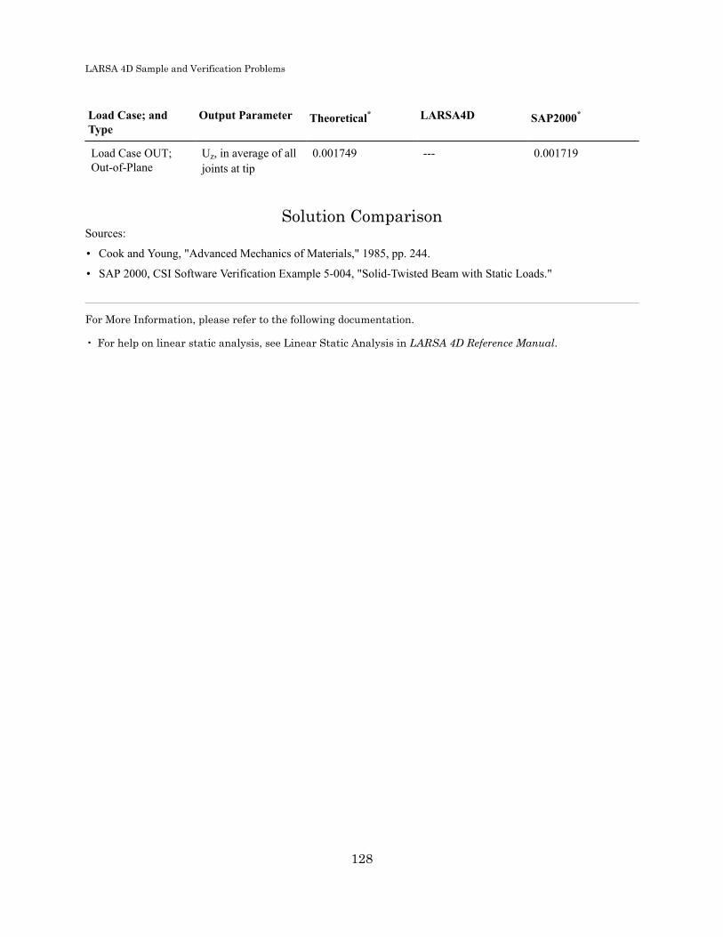
LARSA 4D Sample and Verification Problems
Load Case; andType
Output Parameter Theoretical* LARSA4D SAP2000*
Load Case OUT;Out-of-Plane
Uz, in average of alljoints at tip
0.001749 --- 0.001719
Solution ComparisonSources:
• Cook and Young, "Advanced Mechanics of Materials," 1985, pp. 244.
• SAP 2000, CSI Software Verification Example 5-004, "Solid-Twisted Beam with Static Loads."
For More Information, please refer to the following documentation.
• For help on linear static analysis, see Linear Static Analysis in LARSA 4D Reference Manual.
128

LARSA 4D Sample and Verification Problems
L31: Non-Prismatic Beam withNonlinear Thermal Load
A tapered beam is subjected to a nonlinear thermal gradient load. The behavior of the beam is examined by consideringthree different support conditions: pin-roller, pin-pin, and fix-fix.
Problem DescriptionA beam having a non-prismatic cross-section shape, with its depth varying linearly along its length, is subjected to anonlinear thermal gradient load also along its depth. The beam is 300 ft in length, has a depth that ranges from 1.0 to0.5 feet, and is divided into two elements of equal length. The behavior of the beam is examined by considering threedifferent support conditions: pin-roller, pin-pin, and fix-fix.
Beam Models
A thermal change is applied through the entire depth of the cross-section with formula t = y2, where y is measuredfrom the lower extreme fiber of the section in feet (y is therefore in the range [0, 1]) and t is in °F. The temperaturechange at the top is 1 °F. For the purposes of entering the temperature curve into LARSA 4D, it has been discretizedinto 10 points equally spaced on the section y-axis.
The non-prismatic rectangular cross-section is defined by utilizing the Section Composer tool. The width of the beamis constant and 4 ft. The depth, on the other hand, varies through its length in such a way that it follows the equationd = 1 – x/2, where x is the relative span distance (in the range [0, 1]) and d is the section depth. The cross-sectioncentroid is aligned with the member reference axis along its length. In LARSA 4D, a span is assigned to the two beamelements to obtain the continuous change in depth throughout the whole beam.
129
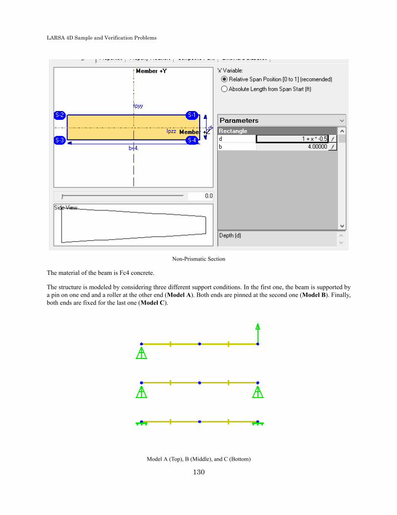
LARSA 4D Sample and Verification Problems
Non-Prismatic Section
The material of the beam is Fc4 concrete.
The structure is modeled by considering three different support conditions. In the first one, the beam is supported bya pin on one end and a roller at the other end (Model A). Both ends are pinned at the second one (Model B). Finally,both ends are fixed for the last one (Model C).
Model A (Top), B (Middle), and C (Bottom)
130
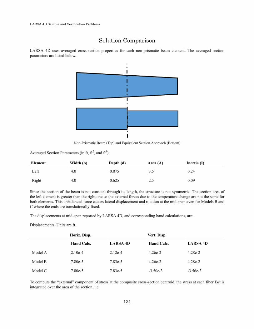
LARSA 4D Sample and Verification Problems
Solution ComparisonLARSA 4D uses averaged cross-section properties for each non-prismatic beam element. The averaged sectionparameters are listed below.
Non-Prismatic Beam (Top) and Equivalent Section Approach (Bottom)
Averaged Section Parameters (in ft, ft2, and ft4)
Element Width (b) Depth (d) Area (A) Inertia (I)
Left 4.0 0.875 3.5 0.24
Right 4.0 0.625 2.5 0.09
Since the section of the beam is not constant through its length, the structure is not symmetric. The section area ofthe left element is greater than the right one so the external forces due to the temperature change are not the same forboth elements. This unbalanced force causes lateral displacement and rotation at the mid-span even for Models B andC where the ends are translationally fixed.
The displacements at mid-span reported by LARSA 4D, and corresponding hand calculations, are:
Displacements. Units are ft.
Horiz. Disp. Vert. Disp.
Hand Calc. LARSA 4D Hand Calc. LARSA 4D
Model A 2.10e-4 2.12e-4 4.26e-2 4.28e-2
Model B 7.80e-5 7.83e-5 4.26e-2 4.28e-2
Model C 7.80e-5 7.83e-5 -3.50e-3 -3.56e-3
To compute the “external” component of stress at the composite cross-section centroid, the stress at each fiber Eαt isintegrated over the area of the section, i.e.
131

LARSA 4D Sample and Verification Problems
F = ∫ Eαy2 da
M = ∫ Eαy2(y-d/2) da
where E and α are the elastic modulus and coefficient of thermal expansion, y is the location of the fiber relative to thelowest fiber of the section, and d/2 is the distance from the lowest fiber to the centroid of the composite section.
Computation of “External” Force and Moment. Units are kip, ft and °F.
Member AverageDepth (dav)
Width (b) ElasticModulus, (E)
α Force (F) Moment (M)
Left 0.875 4.0 519,120 5.50e-6 2.55 0.56
Right 0.625 4.0 519,120 5.50e-6 0.93 0.15
External forces on each node are shown below.
Computation of External Nodal Forces. Units are kip and ft
@ start @ mid-span @ end
Axial Force Moment Axial Force Moment Axial Force Moment
Model A - 0.554 1.621 -0.409 0.929 -0.145
Model B - 0.554 1.621 -0.409 - -0.145
Model C - - 1.621 -0.409 - -
By solving the structure under external nodal forces, we can compute the member end forces as internal forces (Pint:Internal axial force, Mint: Internal Moment).
Internal Forces. Units are kip and ft
@ Left MemberStart
@ Right MemberStart
Pint Mint Pint Mint
Model A 2.55 0.55 0.93 0.15
Model B 0.95 0.55 -0.68 0.15
Model C 0.95 -0.05 -0.68 -0.18
The total stress in each shape is computed in the following table by adding the “external” stress as given by the totalstrains above and the “internal” stress based on the value of the nonlinear curve at the fiber. Note that stress recoverypoint 1 and 3 are at top and bottom fibers, respectively.
Hand Calc. Stress Computation. Units are kip and ft.
132

LARSA 4D Sample and Verification Problems
Model A @ Left MemberStart
@ Right MemberStart
Stress Point 1 Stress Point 3 Stress Point 1 Stress Point 3
y 1.0 0.0 0.75 0.0
(Pint/A) + (Mintc/I) 1.47 -0.19 0.70 -0.08
-Eαy2 -2.86 0.0 -1.61 0.0
Total Stress:
Hand Calc -1.39 -0.19 -0.91 -0.08
LARSA 4D -1.38 -0.20 -0.91 -0.07
Model B @ Left MemberStart
@ Right MemberStart
Stress Point 1 Stress Point 3 Stress Point 1 Stress Point 3
y 1.0 0.0 0.75 0.0
(Pint/A) + (Mintc/I) 1.07 -0.60 0.16 -0.62
-Eαy2 -2.86 0.0 -1.61 0.0
Total Stress:
Hand Calc -1.79 -0.60 -1.45 -0.62
LARSA 4D -1.78 -0.60 -1.45 -0.61
Model C @ Left MemberStart
@ Right MemberStart
Stress Point 1 Stress Point 3 Stress Point 1 Stress Point 3
y 1.0 0.0 0.75 0.0
(Pint/A) + (Mintc/I) 0.16 0.32 -0.70 0.25
-Eαy2 -2.86 0.0 -1.61 0.0
Total Stress:
Hand Calc -2.70 0.32 -2.31 0.25
LARSA 4D -2.71 0.32 -2.32 0.25
133

LARSA 4D Sample and Verification Problems
For More Information, please refer to the following documentation.
• Member Thermal Loads in LARSA 4D Reference Manual.
134
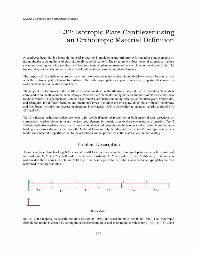
LARSA 4D Sample and Verification Problems
L32: Isotropic Plate Cantilever usingan Orthotropic Material Definition
A cantilever beam having isotropic material properties is modeled using orthotropic formulation plate elements bygiving the the same modulus of elasticity in all loaded directions. The structure is subject to axial extension, in planeshear and bending, out of plane shear and bending, twist, in plane moment and out of plane moment joint loads. Thetip joint displacement is compared to a model with isotropic formulation plate elements.
The purpose of this verification problem is to test the orthotropic material formulation for plate elements by comparisonwith the isotropic plate element formulation. The orthotropic plates are given numerical properties that result inisotropic behavior in the directions loaded.
The tip joint displacements of the cantilever structure modeled with orthotropic material plate formulation elements iscompared to an identical model with isotropic material plate elements having the same modulus of elasticity and shearmodulus values. This comparison is done for different plate shapes including rectangular, parallelogram, trapezoidal,and triangular and different bending and membrane types, including the thin plate, thick plate, bilinear membrane,and membrane with drilling degrees of freedom. The Material UCS is also varied to create a material angle of 11°,45°, and 90°.
Test 1 validates orthotropic plate elements with identical material properties in both material axis directions bycomparison to plate elements using the isotropic element formulation set to the same material properties. Test 2validates orthotropic plate elements with non-identical material properties in the two material axis directions but underloading that causes strain in either only the Material 1 axis or only the Material 2 axis, and the isotropic comparisonmodel uses material properties equal to the orthotropic model properties in the material axis under loading.
Problem DescriptionA cantilever beam 6 inches long, 0.2 inches tall, and 0.1 inches thick is divided into 1-inch plate elements It is restrainedin translation X, Y and Z at bottom-left corner and translation X, Y at top-left corner. Additionally, rotation Z isrestrained at these corners. (Rotation Y DOFs of the beams generated with bilinear membrane type plates are alsorestrained to satisfy stability)
Beam Model
In Test 1, the material has elastic modulus 10,000,000 lb/in2 and shear modulus 4,000,000 lb/in2. The orthotropicformulation model is created by setting the same elastic modulus and shear modulus values for E11, E22, G12, G13, and
135

LARSA 4D Sample and Verification Problems
G23. (Poisson’s ratio, which can be computed from the elastic modulus and shear modulus but must be entered by theuser for orthotropic materials, is 0.25.)
In Test 2, two orthotropic materials are used, each with elastic modulus 10,000,000 lb/in2 in one direction and20,000,000 lb/in2 in the other direction, and other properties as in Test 1. The orthotropic materials are identical exceptthat one has the elastic modulus values in E11 and E22, and the other in E22 and E11 (i.e., reversed).
Test 2 Material Definitions
Material axes are configured using the Material UCS parameter of the materials. In Test 1, the orthotropic materialis repeated three times, and a different User Coordinate System is assigned to each to achieve material angles of 0°,45°, and 90°. (Since the material has identical properties in both directions, the results are expected to be identicalregardless of the material axes, which is one of the results to be verified here.) To obtain the material axis orientationwhere θ=45°, a Material UCS can be as given as:
UCS of 45° Material Angle Plate
136

LARSA 4D Sample and Verification Problems
In Test 2, the material whose E11 matches the E value of the isotropic material (10,000,000 lb/in2) is given a UserCoordinate System such that it gives a material angle of 0°, and the orthotropic material whose E22 matches the E valueof the isotropic material is given a User Coordinate System such that it gives a material angle of 90°, which aligns E22with the applied load. (There is no 45° case in Test 2 because the load would cause strain along both material axes,which could not be compared to an equivalent isotropic model.)
UCS of 90° Material Angle Plate
Four different element shapes are used for comparison: rectangular, trapezoidal, parallelogram and triangular with thegeometric properties shown below:
137
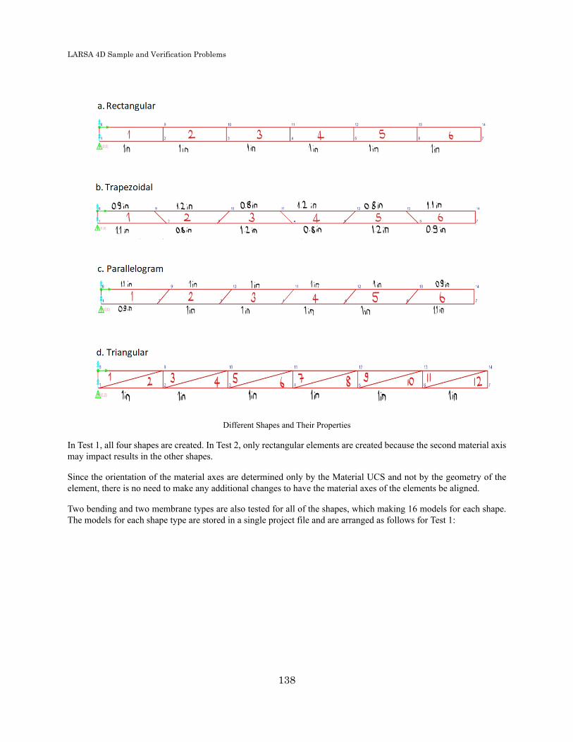
LARSA 4D Sample and Verification Problems
Different Shapes and Their Properties
In Test 1, all four shapes are created. In Test 2, only rectangular elements are created because the second material axismay impact results in the other shapes.
Since the orientation of the material axes are determined only by the Material UCS and not by the geometry of theelement, there is no need to make any additional changes to have the material axes of the elements be aligned.
Two bending and two membrane types are also tested for all of the shapes, which making 16 models for each shape.The models for each shape type are stored in a single project file and are arranged as follows for Test 1:
138

LARSA 4D Sample and Verification Problems
Test 1 Models for the Reactangular Plate
For triangular elements, the Constant Strain Triangle membrane behavior is used in all models.
There are 12 models in Test 2:
Test 2 Models
The load magnitudes of the axial extension, in plane shear and bending, out of plane shear and bending joint loadsare 0.5 lb. Twist and in plane moment loads are 5 lb and out of plane moment is 0.5 lb-in in magnitude. The jointloads are shown below:
139

LARSA 4D Sample and Verification Problems
Loading Conditions
In Test 2, load conditions that cause strain in the second material axis are excluded, leaving axial extension, out ofplane shear and bending, twist, and out of plane moment joint loads.
Solution ComparisonThe tip displacements are compared by taking the average displacements of joint 7 and joint 14, which are the top andbottom joints of the right most plate and percent differences with respect to isotropic case are presented in parenthesis.Example tables of displacements are given below for thin and thick bending type plates, with drilling membrane type.
Test 1
Average Tip Displacements for Rectangular Thick Plates With Drilling Membrane
Load Case OutputParameter
Isotropic Orthotropic 90 Orthotropic 45 Orthotropic 11
1. AxialExtension
U1 (in) 3.00E-05 3.00E-05 3.00E-05 3.00E-05
2. In PlaneShear andBending
U3 (in) 1.06E-01 1.06E-01 1.06E-01 1.06E-01
3. Out of PlaneShear andBending
U2 (in) 4.32E-01 4.32E-01 4.32E-01 4.32E-01
4. Twist U2 (in) 2.94E-03 2.94E-03 2.94E-03 2.94E-03
140
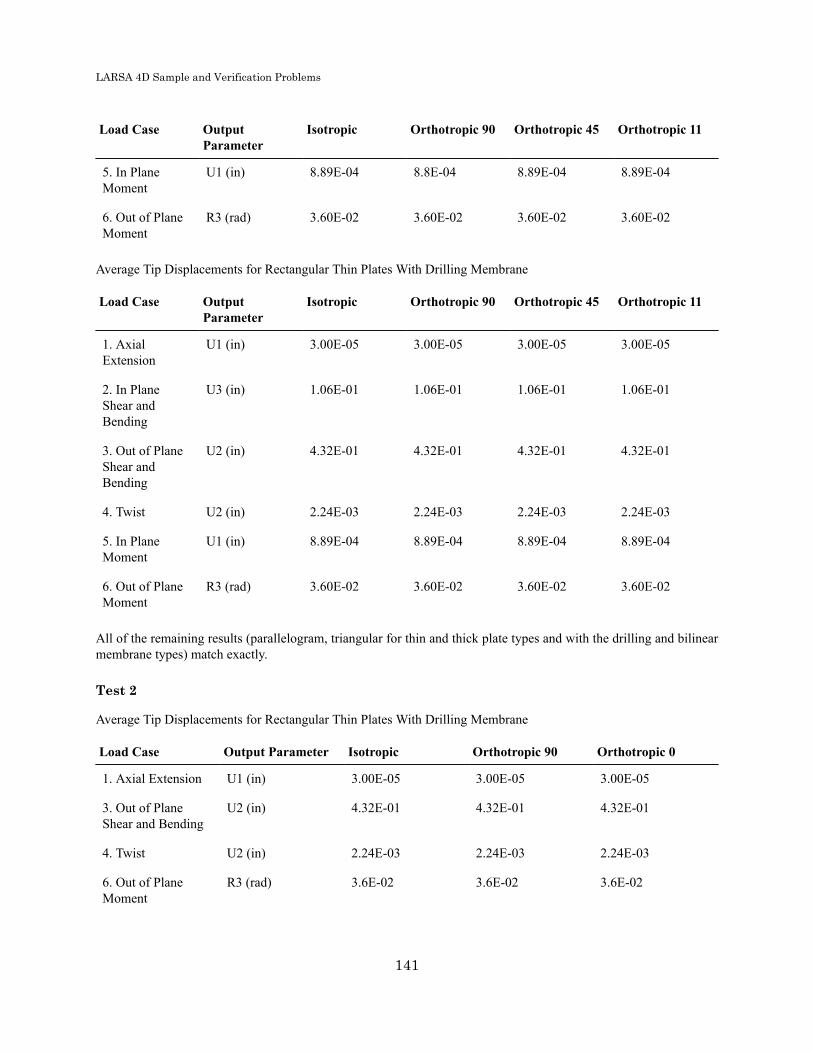
LARSA 4D Sample and Verification Problems
Load Case OutputParameter
Isotropic Orthotropic 90 Orthotropic 45 Orthotropic 11
5. In PlaneMoment
U1 (in) 8.89E-04 8.8E-04 8.89E-04 8.89E-04
6. Out of PlaneMoment
R3 (rad) 3.60E-02 3.60E-02 3.60E-02 3.60E-02
Average Tip Displacements for Rectangular Thin Plates With Drilling Membrane
Load Case OutputParameter
Isotropic Orthotropic 90 Orthotropic 45 Orthotropic 11
1. AxialExtension
U1 (in) 3.00E-05 3.00E-05 3.00E-05 3.00E-05
2. In PlaneShear andBending
U3 (in) 1.06E-01 1.06E-01 1.06E-01 1.06E-01
3. Out of PlaneShear andBending
U2 (in) 4.32E-01 4.32E-01 4.32E-01 4.32E-01
4. Twist U2 (in) 2.24E-03 2.24E-03 2.24E-03 2.24E-03
5. In PlaneMoment
U1 (in) 8.89E-04 8.89E-04 8.89E-04 8.89E-04
6. Out of PlaneMoment
R3 (rad) 3.60E-02 3.60E-02 3.60E-02 3.60E-02
All of the remaining results (parallelogram, triangular for thin and thick plate types and with the drilling and bilinearmembrane types) match exactly.
Test 2
Average Tip Displacements for Rectangular Thin Plates With Drilling Membrane
Load Case Output Parameter Isotropic Orthotropic 90 Orthotropic 0
1. Axial Extension U1 (in) 3.00E-05 3.00E-05 3.00E-05
3. Out of PlaneShear and Bending
U2 (in) 4.32E-01 4.32E-01 4.32E-01
4. Twist U2 (in) 2.24E-03 2.24E-03 2.24E-03
6. Out of PlaneMoment
R3 (rad) 3.6E-02 3.6E-02 3.6E-02
141

LARSA 4D Sample and Verification Problems
For the thin and thick plane bending type, all the results match (both bilinear and with drilling) except for the twistload case result. There is maximum 0.1% difference with respect to isotropic results in twist case. This difference isdue to having greater stiffness in the transverse direction so the orthotropic models become a little bit stiffer than theisotropic ones.
142
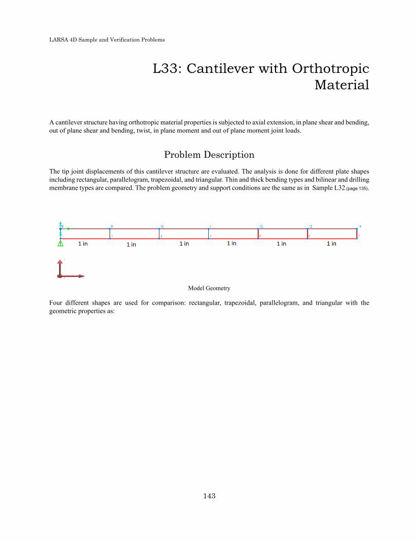
LARSA 4D Sample and Verification Problems
L33: Cantilever with OrthotropicMaterial
A cantilever structure having orthotropic material properties is subjected to axial extension, in plane shear and bending,out of plane shear and bending, twist, in plane moment and out of plane moment joint loads.
Problem DescriptionThe tip joint displacements of this cantilever structure are evaluated. The analysis is done for different plate shapesincluding rectangular, parallelogram, trapezoidal, and triangular. Thin and thick bending types and bilinear and drillingmembrane types are compared. The problem geometry and support conditions are the same as in Sample L32 (page 135).
Model Geometry
Four different shapes are used for comparison: rectangular, trapezoidal, parallelogram, and triangular with thegeometric properties as:
143

LARSA 4D Sample and Verification Problems
Different Shapes and Their Properties
Material properties are:
E11 = 30,000 kip/in2
E22 = 15,000 kip/in2
G12 = 6,600 kip/in2
G13 = 11,693 kip/in2
G22 = 11,693 kip/in2
Poisson's Ratio m12 = 0.2
The load magnitudes of the axial extension, in plane shear and bending, out of plane shear and bending joint loadsare 0.5 lb. Twist and in plane moment loads are 5 lb and out of plane moment is 0.5 lb-in in magnitude. The jointloads are shown below:
144

LARSA 4D Sample and Verification Problems
Loading Conditions
Material axes are configured using the Material UCS parameter of the materials, as shown below. Since the orientationof the material axes are determined only by the Material UCS and not by the geometry of the element, there is no needto make any changes to have the material axes of the elements be aligned.
Material Definitions
As an example, to obtain a θ=45° material angle, the material's local X axis needs to be rotated 45 degrees in counter-clockwise direction. To obtain this material axis orientation, a UCS configuration can be given as:
145

LARSA 4D Sample and Verification Problems
UCS of 45° Material Angle Plate
Different bending and membrane types are tested for all of the shapes separately, which makes 12 different models forthe quadrilateral shapes and 6 different models for the triangular shape, which are layed out as:
Models for the Reactangular Plate
Triangular elements only support the Constant Strain Triangle membrane behavior.
146

LARSA 4D Sample and Verification Problems
For the in plane load cases axial extension, in plane shear and bending and in plane moment, only the membranebehavior of the plate element is relevant. And for out of plane shear and bending, twist, and out of plane moment, onlythe plate bending behavior is relevant.
Solution ComparisonThe tip displacements are compared to SAP2000 V21 results by taking the average displacements of joint 7 and joint14, which are the top and bottom joints of the right-most plate.
Example comparison table of displacements can be seen below for 11 degree material angle rectangular plate for thinbending type and bilinear membrane type:
Load Case Output Parameter LARSA 4D SAP2000 Percent Difference
1. Axial Extension U1 (in) 1.06E-05 1.06E-05 0.0%
2.In Plane Shear andBending
U3 (in) 5.28E-03 5.28E-03 0.0%
3. Out of PlaneShear and Bending
U2 (in) 1.53E-01 1.53E-01 0.0%
4. Twist U2 (in) 5.64E-03 5.64E-03 0.0%
5. In Plane Moment U1 (in) 4.39E-05 4.39E-05 0.0%
6. Out of PlaneMoment
R3 (rad) 1.27E-02 1.27E-02 0.0%
Example comparison table of displacements for triangular mesh can be seen below for 11 degree material angle platefor thin bending type and bilinear membrane type:
Load Case Output Parameter LARSA 4D SAP2000 Percent Difference
1. Axial Extension U1 (in) 1.06E-05 1.06E-05 0.0%
2.In Plane Shear andBending
U3 (in) 2.03E-03 2.03-03 0.0%
3. Out of PlaneShear and Bending
U2 (in) 1.52E-01 1.52E-01 0.0%
4. Twist U2 (in) 5.52E-03 5.52E-03 0.0%
5. In Plane Moment U1 (in) 1.66E-05 1.66E-05 0.0%
6. Out of PlaneMoment
R3 (rad) 1.27E-02 1.27E-02 0.0%
LARSA 4D’s bilinear membrane behavior matched SAP 2000’s plane stress plate element exactly for all shape types,material angles, and in-plane loading conditions. On the other hand, there are up to 35% difference between LARSA4D’s drilling membrane behavior and SAP 2000’s shell elements for meshes with trapezoidal and parallelogram
147

LARSA 4D Sample and Verification Problems
elements. Similar differences can also be observed from the comparison of isotropic material behavior given in L18(page 61).
LARSA 4D’s thin plate bending behavior matched SAP 2000’s thin shell element exactly for all shape types, materialangles, and out-of-plane loading conditions. LARSA 4D’s thick plate bending behavior matched SAP 2000’s thickshell element with insignificant differences (0-1.5%) in out-of-plane shear, bending, and moment (but not twist) for allshape types and material angles. In the thick plate twist cases, significant differences between LARSA 4D and SAP2000 were found. However, LARSA 4D’s thick plate has comparable results to LARSA 4D’s thin plate in all twistcases, and in many cases the LARSA 4D results and the SAP 2000 results are believed to be equidistant from the truesolution which indicates the current mesh density is not sufficient to represent the deformed shape for twisting.
148

LARSA 4D Sample and Verification Problems
L35: Plate Initial Strain Load
A cylinder is analyzed for a 25°F uniform temperature load. The same loading is also represented by an equivalentinitial strain load applied to the plate elements. Displacements in vertical direction and plate internal forces arecompared.
Problem DescriptionThe cylinder is 200 inches tall and has a 60 inch radius. The wall thickness is 1 inch. Geometry of the structure is thesame as the 8x16 model discussed in sample L20 (page 73) except the support conditions.
Model Geometry
Material properties are:
E = 29,000 kip/in2
Poisson's Ratio = 0.0
G = 14,500 kip/in2
Thermal Expansion Coef. = 6.5x10⁻⁶ 1/°F
149
LARSA 4D Sample and Verification Problems
The displacement directions of all joints are oriented such that axis 1 points radially outward and axis 3 points upward.The joints at the base of the cylinder are restrained against translation in the local 1 and 3 directions but one of themis restrained in local 2 direction also. All the other joints are restrained against translation in the local 1 direction only.The local axes of all the shells are oriented such that axis 3 points radially outward and axis 2 points upward.
The structure is subjected to 25oF uniform temperature change. This temperature change load is also in a separatemodel represented by an equivalent strain load of 1.625x10⁻⁴ (computed as the coefficient of thermal expansion timesthe temperature change) on each plate element in both local x and y directions.
Solution ComparisonSolutions are compared for the Bilinear, Incompatible, and Drilling plate membrane behaviors and the MITC4 behaviorfor quadrilateral elements and the Bilinear membrane behavior for triangular elements. (Since the loading is relatedto in plane behavior only, only membrane behavior is considered.) The thermal load and the initial strain load arealso compared.
The top displacement and the plate internal forces are compared from any of the joint at top and any of the plate,respectively.
Quadrilateral Bilinear Plate
Parameter Uniform Temperature Initial Strain
local U3 (in) 0.0325 0.0325
F11 (lb/in) -4712.50 -4712.50
Quadrilateral Incompatible Plate
Parameter Uniform Temperature Initial Strain
local U3 (in) 0.0325 0.0325
F11 (lb/in) -4712.50 -4712.50
Quadrilateral Drilling Plate
Parameter Uniform Temperature Initial Strain
local U3 (in) 0.0325 0.0325
F11 (lb/in) -4712.50 -4712.50
Quadrilateral MITC4 Plate
Parameter Uniform Temperature Initial Strain
local U3 (in) 0.0325 0.0325
F11 (lb/in) -4712.50 -4712.50
150

LARSA 4D Sample and Verification Problems
Triangular Bilinear Plate
Parameter Uniform Temperature Initial Strain
local U3 (in) 0.0325 0.0325
F11 (lb/in) -4712.50 -4712.50
Initial strain case results match with the uniform temperature load case results for all models, perfectly.
The same example is repeated by using staged construction analysis. The total initial strain is applied within twoseparate stages in such a way that half strain is applied in both stages (i.e. 1/2 in first stage and the remaining 1/2 inthe next stage). At the end of the final stage, the same displacements and internal forces are obtained.
151

LARSA 4D Sample and Verification Problems
152

LARSA 4D Sample and Verification Problems
Samples for Nonlinear ElasticStatic Analysis
These samples provide an overview of the nonlinear elastic static analysis.
N01: Tie Beam with Geometric Stiffening 155Solution Comparison 156Reference 156
N02: Cable with Hanging Loads 157Solution Comparison 157
N03: Beam on an Elastic Soil Foundation 159Solution Comparison 159Reference 160
N04: Truss with Misaligned Supports - Nonlinear Static 161Solution Comparison 161
N05: Nonlinear Analysis of Cable Roof 163Solution Comparison 163
N06: Diamond Shaped Frame - Geometric Nonlinear 165Reference 166Solution Comparison 166
N07: Diamond Shaped Frame - Geometric Nonlinear - IncrementalJoint Displacement Loading
167
Reference 168Solution Comparison 168
N08: A High Arch Structure - Geometric Nonlinear 169Solution Comparison 170Reference 170
N09: Thermal Expansion to Close a Gap 171Solution Comparison 171
N13: Straight Cantilever Girder with Nonlinear Shell Elements inMembrane Action
173
Problem Description 173Solution Comparison 174References 175
153

LARSA 4D Sample and Verification Problems
N14: Straight Cantilever Girder with Nonlinear Shell Elements inPlate Action
177
Problem Description 177Solution Comparison 178References 179
N15: Slit Annular Plate with Vertical Load 181Problem Description 181Solution Comparison 182References 183
154

LARSA 4D Sample and Verification Problems
N01: Tie Beam with GeometricStiffening
A tie beam is subjected to the action of a tensile force and a uniform lateral load. The tensile force is 21,970 lb and theuniform lateral load is 1.79258 lb/in. The beam is steel and has a square section of 2.5 in by 2.5 in.
Determine the maximum deflection, maximum bending moment and the slope at the lefthand support. In this sample,the effect of geometric stiffening is included by using nonlinear static analysis and compare the results to those inproblem 10 where the geometric nonlinearity is ignored. Also, for this sample problem, two different finite models arecreated to see the behavior of beam element and nonlinear shell element (MITC4), seperately.
Example Project: The example described here can be found in the Nonlinear Elastic Static folder of your LARSA4D Samples directory (generally My Documents\LARSA Projects\Samples) in the file N01.
Sample N01
The first model has 9 joints and 8 beam elements. The second one has 18 joints and 8 shell elements. The tensile forceis specified as an external force acting at joint 9 for the first model and joint 17 and joint 18 for the second model.The uniform load is specified as an external beam loading and external plate loading for the first and second model,respectively. For the second model, shells are placed in out of plane action. Also, as plate and membrane type, MITC4is used to get nonlinear behavior.
Modulus of Elasticity = 30,000,000 lb/in2
Span = 200 inches
A = 6.25 in2
Izz = 3.2552 in4
155

LARSA 4D Sample and Verification Problems
Uniform Load = 1.79253 lb/in
Tensile Force S = 21,970 lb
Nonlinear static analysis is performed using one (1) load step and maximum of 20 iterations.
Solution Comparison
Timoshenko Beam Shell
Vertical Disp @ Node 5(in)
-0.200 -0.1995 -0.1970
Rotation @ Joint 1(rad) -0.0032352 -0.003236 -0.003218
Moment @ I-end of Beam5(in-lb)
-4579.91 -4580.29 -4514.73
The nonlinear static analysis includes the geometric stiffening effect of the beam. For comparison of results to thelinear static analysis, refer to the previous problem.
Reference• Timoshenko, S., "Strength of Materials, Part II", 3rd Edition, D. Van Nostrand Co., Inc., New York, p. 42.
For More Information, please refer to the following documentation.
• For help on Nonlinear Elastic Static analysis, see Nonlinear Static Analysis in LARSA 4D Reference Manual.
156

LARSA 4D Sample and Verification Problems
N02: Cable with Hanging Loads
The cable supports three vertical loads. The area of the cable is 0.1 ft2. The elastic modulus of the cable is 200,000kips/ft2.
Determine the reaction forces and the maximum tension in the cable.
Example Project: The example described here can be found in the Nonlinear Elastic Static folder of your LARSA4D Samples directory (generally My Documents\LARSA Projects\Samples) in the file N02.
The model has 5 joints and 4 cable elements. A small tensile force
Sample 12
is specified as prestress force to give initial stiffness to the cable.
Modulus of Elasticity = 200,000 kips/ft2
A = 0.10 ft2
Initial Tensile Force = .10 kips
Solution ComparisonSources:
• LARSA 4D
• Beer and Johnston, page 260.LARSA Beer
Reaction Ax (kips) -17.89 -17.9
Reaction Az (kips) +5.03 +5.03
Reaction Bz (kips) 16.97 16.97
Max Cable Tension (kips) 24.66 24.70
The tension in the cable varies from 17.9 kips (element # 2) to 24.7 kips (element # 4).
For More Information, please refer to the following documentation.
• For help on Nonlinear Elastic Static analysis, see Nonlinear Static Analysis in LARSA 4D Reference Manual.
157

LARSA 4D Sample and Verification Problems
158
LARSA 4D Sample and Verification Problems
N03: Beam on an Elastic SoilFoundation
A 30-inch long beam rests on an elastic foundation. The beam is 3 inches wide and 1 inch deep. The soil is active incompression only. The foundation modulus is 5000 lb/cubic inch. A concentrated load of 8000 lbs is applied at themidspan of the beam. For this sample problem, two different finite models are created to see the behavior of beamelement and nonlinear shell element (MITC4), seperately.
Determine the midspan displacement and the contact length of the beam.
Example Project: The example described here can be found in the Nonlinear Elastic Static folder of your LARSA4D Samples directory (generally My Documents\LARSA Projects\Samples) in the file N03.
Sample N03
The material and section property data of the beam are:
Modulus of Elasticity = 30,000,000 lb/in2
Poisson's Ratio = 0.00
Izz = 0.25 in4
A = 3 in2
There are two models which are modeled with different element types. The first model has beam and compression-only foundation spring elements. The second model has shell and compression-only foundation spring elements.Due to symmetry, only one half of the structure is modeled.
The beam is divided into 10 equal length beam and shell elements for first and second model, respectively. Thefoundation is modeled using the compression-only foundation spring elements. The spring constant (K) is taken asfoundation modulus times the beam width times the spacing between the springs.
K = (Foundation Modulus) x Contact Area
K = 5000 x 3 x 1.5
K = 22,500 lb/in.
Solution ComparisonThe results for the displacement under the load and the extent of the contact are compared to the exact solution byHeteyni and to the solution from NISA.
The displacement reported is in the direction of the load (-Z direction) at the point of application of the load and theresults are in inches.
The contact length is computed by linear interpolation of the vertical displacement over the beam segment in whichthe deflection changes sign.
159

LARSA 4D Sample and Verification Problems
Heteyni NISA Beam Shell
Displacement 0.043480 0.043478 0.043478 0.044193
Half length ofcontact
10.505 10.546 10.546 10.534
The comparison of the results is excellent.
Reference• Faten F. Mahmoud, N.J. Slamon and W.R. Marks, "A Direct Automated Procedure for Frictionless Contact
Problems", International Journal of Numerical Methods Eng., 18 (1982), pp. 245-257.
• M. Heteyni, "Beams on Elastic Foundation", University of Michigan Press, Ann Arbor, Michigan, 1967.
• NISA, Verification Problems Manual, EMRC, 1990
For More Information, please refer to the following documentation.
• For help on Nonlinear Elastic Static analysis, see Nonlinear Static Analysis in LARSA 4D Reference Manual.
160

LARSA 4D Sample and Verification Problems
N04: Truss with MisalignedSupports - Nonlinear Static
A 1000 inch span truss has six flexible supports. The four interior supports are misaligned. The truss is subjected tofour point loads at the lower chord.
Determine the vertical displacements at the joints along the bottom chord of the truss and the final gap widths.
Example Project: The example described here can be found in the Nonlinear Elastic Static folder of your LARSA4D Samples directory (generally My Documents\LARSA Projects\Samples) in the file N04.
Sample N04
Truss elements of constant cross section are used to model the structure. The material and section property of thetruss is:
Modulus of Elasticity = 30,000,000 lb/in2
Poisson's Ratio = 0.00
Area = 10 in2
The misalignments of the interior supports are modeled using compression-only foundation spring with built-in gapelement.
K = 1,000,000 lb/in
Gap Distance @ Joint 2= 0.80 inch
Gap Distance @ Joint 3= 0.90 inch
Gap Distance @ Joint 4= 1.20 inch
Gap Distance @ Joint 5= .50 inch
The exterior supports have no misalignment and the gap distance is specified as zero.
K = 1,000,000,000 lb/in
The joint at the top center of the truss is restrained from moving in the horizontal direction. Only the vertical movementis allowed at the center supports.
Concentrated forces of 40,000 lbs each are applied at the interior joints of the bottom chord of the truss.
Solution ComparisonJoint Displacements (inch)Sources:
• W.R. Marks, "Solution of Frictionless Contact Problems by a Conjugate Gradient Technique,", M.Sc. Thesis,University of Wisconsin, Milwaukee (1979).
• EMRC, "NISA II Verification Problems Manual", 1991.
161

LARSA 4D Sample and Verification Problems
• LARSA 4DMarks EMRC LARSA
X Displacement
Node 2 -0.11801 -0.11779
Node 3 -0.03822 -0.03823
Node 4 -0.05359 -0.05361
Node 5 0.12368 0.12340
Z Displacement
Node 2 -0.59902 -0.59902
Node 3 -0.91924 -0.91926
Node 4 -0.90721 -0.90722
Node 5 -0.53625 -0.53627
Extent of Gap (inch)
Node 2 InitialGap=0.8 No Contact No Contact No Contact
Node 3 InitialGap=0.9 -0.019241 -0.019241 -0.01926
Node 4 InitialGap=1.2 No Contact No Contact No Contact
Node 5 InitialGap=0.5 -0.036254 -0.036254 -0.036266
Interior Support ReactionForces (kips)
Node 2 0 0 0
Node 3 19.24 19.24 19.26
Node 4 0 0 0
Node 5 36.25 36.25 36.27
For More Information, please refer to the following documentation.
• For help on Nonlinear Elastic Static analysis, see Nonlinear Static Analysis in LARSA 4D Reference Manual.
162

LARSA 4D Sample and Verification Problems
N05: Nonlinear Analysis of CableRoof
An orthogonal cable network with hyperbolic paraboloid shape is subjected to point loads.
Determine the displacements.
Example Project: The example described here can be found in the Nonlinear Elastic Static folder of your LARSA4D Samples directory (generally My Documents\LARSA Projects\Samples) in the file N05.
Sample N05
The roof is modeled by a finite element mesh of 80 cable elements and 41 joints. The joints on the outer boundaryare fixed.
The material and sectional properties of the cables are:
Modulus of Elasticity = 24,000,000 lb/in2
Area = 1.0 in2
Solution ComparisonVertical Displacement in negative Z Direction (feet)Sources:
• LARSA 4D
• G.R. Monforton and N.M. El-Hakim, "Analysis of Truss- Cable Structures", Computers & Structures,
• EMRC, "NISA II Verification Problems Manual", 1991.LARSA Monforton EMRC
Joint 1 0.440 0.441 0.443
Joint 3 1.370 1.371 1.367
Joint 7 3.752 3.752 3.719
Joint 13 1.669 1.669 1.671
Joint 19 0.961 0.962 0.969
Joint 23 0.559 0.561 0.567
Joint 25 0.223 0.224 0.228
Joint 26 0 0 0
Joint 34 0 0 0
The LARSA results are in excellent agreement with the energy search solution of Ref [1] and they are in good agreementwith the NISA computer program results.
163

LARSA 4D Sample and Verification Problems
For More Information, please refer to the following documentation.
• For help on Nonlinear Elastic Static analysis, see Nonlinear Static Analysis in LARSA 4D Reference Manual.
164

LARSA 4D Sample and Verification Problems
N06: Diamond Shaped Frame -Geometric Nonlinear
A large diamond shape structure with two pin joints and two rigid joints is subjected to a compressive load at the twoopposite corners.
Determine the load-displacement curve at the point of load application for applied load up to 40,000 lbs.
Example Project: The example described here can be found in the Nonlinear Elastic Static folder of your LARSA4D Samples directory (generally My Documents\LARSA Projects\Samples) in the file N06.
Sample N06
The material properties for the frame are:Modulus of Elasticity = 30,000,000 psi
Poisson's Ratio = 0.0
Shear Modulus = 15,000,000 psi
The section properties for the frame are:Axx = 1.0 in2
Iyy = 0.08333 m4
165

LARSA 4D Sample and Verification Problems
Izz = 0.08333 m4
In primary load case 1, point loads of 1,000 lbs each are applied at the top and bottom points of the frame.F1 -Z = -1,000 lb
F3-Z = +1,000 lb
20 equal load increments are defined for computing the loaddeflection behavior of the structure from P = 2,000 to P= 40,000 lbs. The load-deflection option is used in defining the load combination data.
The finite element model consists of 120 beam elements and 120 joints.
Reference• T. J. R. Hughes and W. K. Lui,"Nonlinear Finite Element Analysis of Shells - Part II: Two Dimensional
Shells", Comp. Meth. Appl. Mech. Eng., 27 (1981), 167-181.
• EMRC, "NISA II Verification Problems Manual", 1991.
Solution ComparisonThe load-displacement curves are calculated for the vertical and horizontal displacements of the structure. The verticaldisplacement is at the top and bottom corners of the structure. The horizontal displacement is at the mid-left and rightcorners of the structure.
The values computed by LARSA are in excellent agreement with the experimental results of Hughes and with thenumerical results from EMRC.
For More Information, please refer to the following documentation.
• N07: Diamond Shaped Frame - Geometric Nonlinear - Incremental Joint Displacement Loading on page167.
• For help on Nonlinear Elastic Static analysis, see Nonlinear Static Analysis in LARSA 4D Reference Manual.
166

LARSA 4D Sample and Verification Problems
N07: Diamond Shaped Frame -Geometric Nonlinear - Incremental
Joint Displacement Loading
A large diamond shape structure with two pin joints and two rigid joints is subjected to a compressive load at the twoopposite corners.
Determine the load-displacement curve at the point of load application using incremental joint displacement loading.
Example Project: The example described here can be found in the Nonlinear Elastic Static folder of your LARSA4D Samples directory (generally My Documents\LARSA Projects\Samples) in the file N07.
In N06: Diamond Shaped Frame - Geometric Nonlinear (page 165), the load-displacement behavior was computed usingincremental applied joint loading.
Sample N07
The material properties for the frame are:Modulus of Elasticity = 30,000,000 psi
Poisson's Ratio = 0.0
Shear Modulus = 15,000,000 psi
The section properties for the frame are:Axx = 1.0 in2
167

LARSA 4D Sample and Verification Problems
Iyy = 0.08333 m4
Izz = 0.08333 m4
In primary load case 1, joint displacement loads of 1 inch each are applied at the top and bottom points of the frame.F1 -Z = -1 inch
F3-Z = +1 inch
20 equal load increments are defined for computing the loaddeflection behavior of the structure. The load-deflectionoption is used in defining the load combination data.
The finite element model consists of 120 beam elements and 120 joints.
Reference• T. J. R. Hughes and W. K. Lui, "Nonlinear Finite Element Analysis of Shells - Part II: Two Dimensional
Shells", Comp. Meth. Appl. Mech. Eng., 27 (1981), 167-181.
• EMRC, "NISA II Verification Problems Manual", 1991.
Solution ComparisonThe load-displacement curves are calculated for the vertical and horizontal displacements of the structure. The verticaldisplacement is at the top and bottom corners of the structure. The horizontal displacement is at the mid-left and rightcorners of the structure.
The values computed by LARSA are in excellent agreement with the experimental results of Hughes and with thenumerical results from EMRC.
For More Information, please refer to the following documentation.
• For help on Nonlinear Elastic Static analysis, see Nonlinear Static Analysis in LARSA 4D Reference Manual.• N06: Diamond Shaped Frame - Geometric Nonlinear on page 165.
168
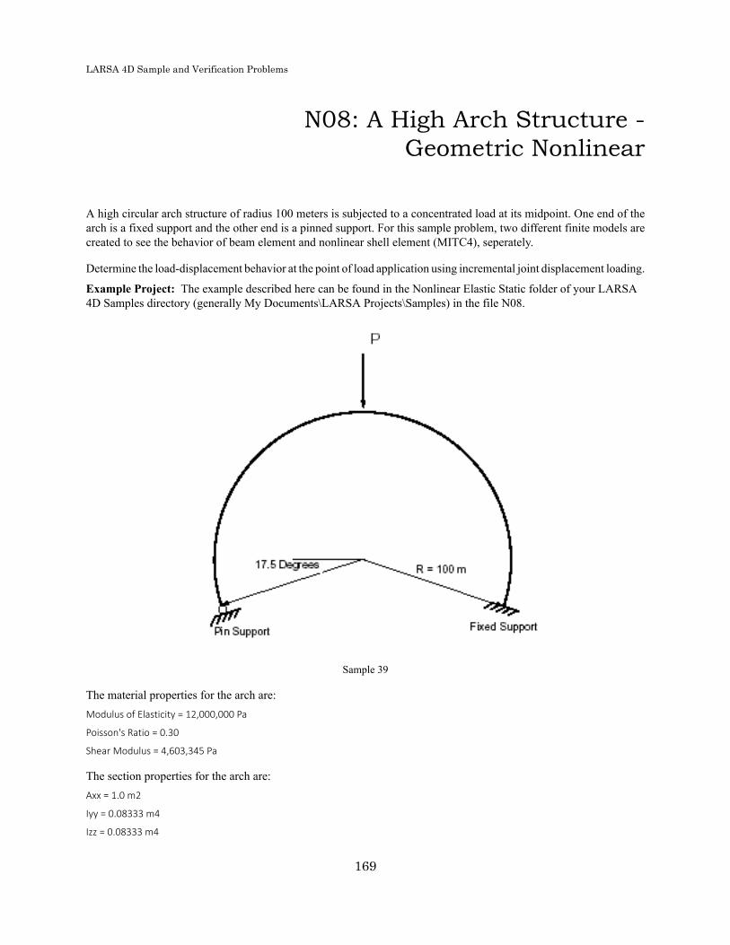
LARSA 4D Sample and Verification Problems
N08: A High Arch Structure -Geometric Nonlinear
A high circular arch structure of radius 100 meters is subjected to a concentrated load at its midpoint. One end of thearch is a fixed support and the other end is a pinned support. For this sample problem, two different finite models arecreated to see the behavior of beam element and nonlinear shell element (MITC4), seperately.
Determine the load-displacement behavior at the point of load application using incremental joint displacement loading.
Example Project: The example described here can be found in the Nonlinear Elastic Static folder of your LARSA4D Samples directory (generally My Documents\LARSA Projects\Samples) in the file N08.
Sample 39
The material properties for the arch are:Modulus of Elasticity = 12,000,000 Pa
Poisson's Ratio = 0.30
Shear Modulus = 4,603,345 Pa
The section properties for the arch are:Axx = 1.0 m2
Iyy = 0.08333 m4
Izz = 0.08333 m4
169
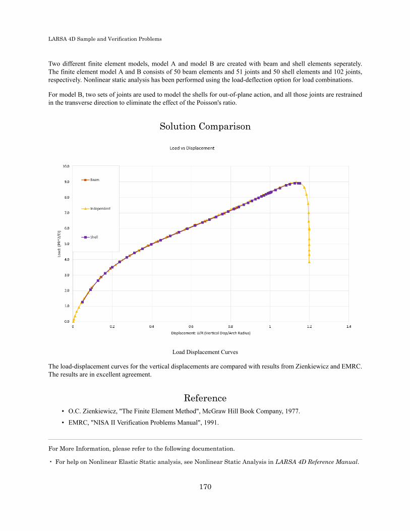
LARSA 4D Sample and Verification Problems
Two different finite element models, model A and model B are created with beam and shell elements seperately.The finite element model A and B consists of 50 beam elements and 51 joints and 50 shell elements and 102 joints,respectively. Nonlinear static analysis has been performed using the load-deflection option for load combinations.
For model B, two sets of joints are used to model the shells for out-of-plane action, and all those joints are restrainedin the transverse direction to eliminate the effect of the Poisson's ratio.
Solution Comparison
Load Displacement Curves
The load-displacement curves for the vertical displacements are compared with results from Zienkiewicz and EMRC.The results are in excellent agreement.
Reference• O.C. Zienkiewicz, "The Finite Element Method", McGraw Hill Book Company, 1977.
• EMRC, "NISA II Verification Problems Manual", 1991.
For More Information, please refer to the following documentation.
• For help on Nonlinear Elastic Static analysis, see Nonlinear Static Analysis in LARSA 4D Reference Manual.
170
LARSA 4D Sample and Verification Problems
N09: Thermal Expansion to Close aGap
An aluminum-alloy bar is initially at a temperature of 70 degrees F. Calculate the stress in the bar after it has beenheated to 170 degrees F. The supports are assumed to be rigid. There is a gap between the support and the end jointof the bar. The gap distance is 0.002 in.
Example Project: The example described here can be found in the Nonlinear Elastic Static folder of your LARSA4D Samples directory (generally My Documents\LARSA Projects\Samples) in the file N09.
The material properties for the bar are:Modulus of Elasticity = 10,500,000 psi
Coefficient of Thermal Expansion = 0.0000125
The section property for the bar is:Axx = 1.0 in2
The finite element model consists of 1 truss element and 1 nonlinear foundation element with built-in gap and spring.The spring stiffness is arbitrarily selected at a high value. Nonlinear static analysis is performed.
To run this model in LARSA 4D with settings compatible with the reference software ANSYS, use Staged ConstructionAnalysis with geometric nonlinearity turned off.
Solution ComparisonSources:
• LARSA 4D with geometric nonlinearity turned on
• LARSA 4D with geometric nonlinearity turned off
• Swanson Analysis Systems, "ANSYS Verification Problems Manual".LARSA-wGN LARSA-woGN Swanson
Stress (psi) -6,1338 -6,125 -6,125
The comparison of the results is excellent.
For More Information, please refer to the following documentation.
• For help on Nonlinear Elastic Static analysis, see Nonlinear Static Analysis in LARSA 4D Reference Manual.
171

LARSA 4D Sample and Verification Problems
172
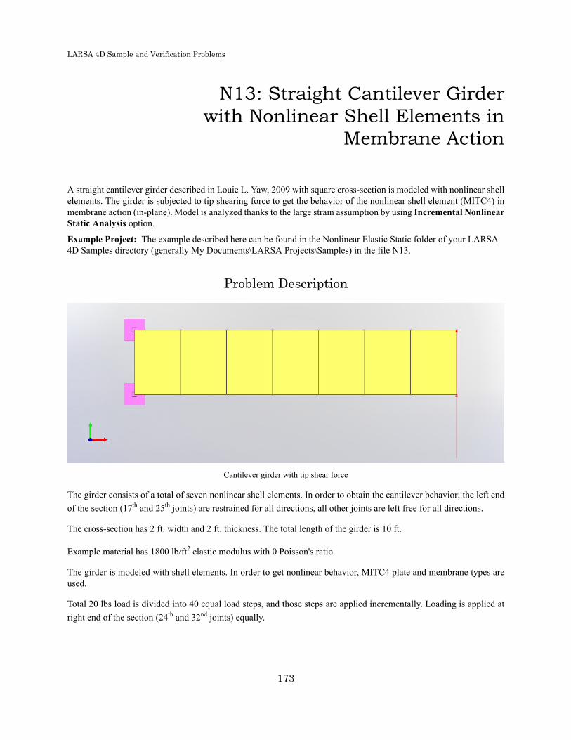
LARSA 4D Sample and Verification Problems
N13: Straight Cantilever Girderwith Nonlinear Shell Elements in
Membrane Action
A straight cantilever girder described in Louie L. Yaw, 2009 with square cross-section is modeled with nonlinear shellelements. The girder is subjected to tip shearing force to get the behavior of the nonlinear shell element (MITC4) inmembrane action (in-plane). Model is analyzed thanks to the large strain assumption by using Incremental NonlinearStatic Analysis option.
Example Project: The example described here can be found in the Nonlinear Elastic Static folder of your LARSA4D Samples directory (generally My Documents\LARSA Projects\Samples) in the file N13.
Problem Description
Cantilever girder with tip shear force
The girder consists of a total of seven nonlinear shell elements. In order to obtain the cantilever behavior; the left endof the section (17th and 25th joints) are restrained for all directions, all other joints are left free for all directions.
The cross-section has 2 ft. width and 2 ft. thickness. The total length of the girder is 10 ft.
Example material has 1800 lb/ft2 elastic modulus with 0 Poisson's ratio.
The girder is modeled with shell elements. In order to get nonlinear behavior, MITC4 plate and membrane types areused.
Total 20 lbs load is divided into 40 equal load steps, and those steps are applied incrementally. Loading is applied atright end of the section (24th and 32nd joints) equally.
173

LARSA 4D Sample and Verification Problems
Deflected Shape
Solution ComparisonAs a result, avarage lateral displacement (Uy) at the tip of the girder is obtained. For the sake of comparison, resultswhich are given by ADINA is listed.
The results of the first 20 steps are listed below. Unit of the results is "feet".
Step Parameter LARSA 4D ADINA Difference
1 Uy 1.01 1.01 0%
2 Uy 1.96 1.96 0%
3 Uy 2.82 2.82 0%
4 Uy 3.57 3.57 0%
5 Uy 4.22 4.22 0%
6 Uy 4.77 4.77 0%
174

LARSA 4D Sample and Verification Problems
Step Parameter LARSA 4D ADINA Difference
7 Uy 5.23 5.23 0%
8 Uy 5.63 5.63 0%
9 Uy 5.97 5.97 0%
10 Uy 6.26 6.26 0%
11 Uy 6.51 6.51 0%
12 Uy 6.73 6.73 0%
13 Uy 6.93 6.93 0%
14 Uy 7.10 7.10 0%
15 Uy 7.26 7.26 0%
16 Uy 7.40 7.40 0%
17 Uy 7.53 7.53 0%
18 Uy 7.64 7.64 0%
19 Uy 7.75 7.75 0%
20 Uy 7.84 7.84 0%
References• Yaw, L. L. (2009). 1 2D Corotational Beam Formulation.
• ADINA R&D, Inc: ADINA 9.6.0 (April 2020)
For More Information, please refer to the following documentation.
• For help on nonlinear static analysis, see Nonlinear Static Analysis in LARSA 4D Reference Manual.• For help on nonlinear plate elements, see Plates in LARSA 4D Reference Manual.
175

LARSA 4D Sample and Verification Problems
176

LARSA 4D Sample and Verification Problems
N14: Straight Cantilever Girder withNonlinear Shell Elements in Plate
Action
A straight cantilever girder with a rectangular cross-section is modeled with nonlinear shell elements. The girder issubjected to tip moment force to get the behavior of the nonlinear shell element (MITC4) in plate action (out-of-plane).Model is analyzed thanks to the large strain assumption by using Incremental Nonlinear Static Analysis option.
Example Project: The example described here can be found in the Nonlinear Elastic Static folder of your LARSA4D Samples directory (generally My Documents\LARSA Projects\Samples) in the file N14.
Problem Description
Cantilever girder with tip moment force
The girder consists of a total of 16 nonlinear shell elements. In order to obtain the cantilever behavior; the left end ofthe section (1st and 2nd joints) are restrained for all directions. In addition to that, all joints are restrained for drillingmotion in the following manner. Since the displacement coordinate system of joints is the global coordinate system,the direction of the drilling degrees of freedom changes under the deformation of the model. Therefore, the model isrestrained in both rotational x and z directions.
The cross-section has 1 in. width and 0.1 in. thickness. The total length of the girder is 12 in.
Example material has 1,200,000 lb/in2 elastic modulus with 0 Poisson's ratio.177

LARSA 4D Sample and Verification Problems
The girder is modeled with shell elements. In order to get nonlinear behavior, MITC4 plate and membrane types areused.
The total 52.36 lb-in load is divided into 20 equal load steps, and those steps are applied incrementally. Loading isapplied at the right end of the section (33rd and 34th joints) equally.
Deflected shape
Solution ComparisonAs a result, average axial and vertical displacement (Ux and Uz) at the tip of the girder is obtained. For the sake ofcomparison, results which are given by ADINA are shown in the figure below.
Results of the 20 steps are shown below. Results are in inches.
178
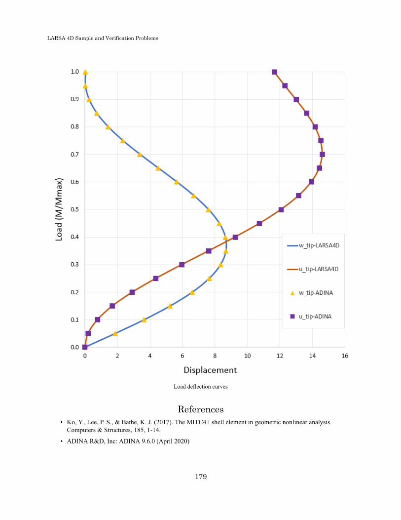
LARSA 4D Sample and Verification Problems
Load deflection curves
References• Ko, Y., Lee, P. S., & Bathe, K. J. (2017). The MITC4+ shell element in geometric nonlinear analysis.
Computers & Structures, 185, 1-14.
• ADINA R&D, Inc: ADINA 9.6.0 (April 2020)
179

LARSA 4D Sample and Verification Problems
For More Information, please refer to the following documentation.
• For help on nonlinear static analysis, see Nonlinear Static Analysis in LARSA 4D Reference Manual.• For help on nonlinear plate elements, see Plates in LARSA 4D Reference Manual.
180

LARSA 4D Sample and Verification Problems
N15: Slit Annular Plate with VerticalLoad
A slit annular plate is modeled by nonlinear elements. The annular plate is meshed 5x40 times in polar coordinate. Theplate is subjected to tip shearing force. Model is analyzed thanks to the large strain assumption by using IncrementalNonlinear Static Analysis option.
Example Project: The example described here can be found in the Nonlinear Elastic Static folder of your LARSA4D Samples directory (generally My Documents\LARSA Projects\Samples) in the file N15.
Problem Description
Slit Annular Plate with 5*40 mesh
The model consists of total 200 nonlinear shell elements. The boundary condition of the model is as follows ; 1st,42nd,83rd, 124th, 165th and 206th joints are restrained for all directions, all other joints are left free for all directions.
Dimensions of the model are as follows;
R0 = 10.0 ft
R1 =6.0 ft
Thickness = 0.03 ft
Example material has 21,000,000 kips/ft2 elastic modulus with 0 Poisson's ratio.
181

LARSA 4D Sample and Verification Problems
The girder is modeled with shell elements. In order to get nonlinear behavior, MITC4 plate and membrane types areused.
Total 5 kips load is divided into 100 equal load steps and those steps are applied incrementally. Loading is applied at41st, 82nd, 123rd, 164th, 205th and 246th joints of the section.
Deflected shape
Solution ComparisonThe load-displacement curve of model is shown below. The curve contains both results of MITC4 and independentresults for comparison.
182

LARSA 4D Sample and Verification Problems
Load-displacement curve
Results are in excellent agreement with independent results.
References• Ko, Y., Lee, P. S., & Bathe, K. J. (2017). The MITC4+ shell element in geometric nonlinear analysis.
Computers & Structures, 185, 1-14.
For More Information, please refer to the following documentation.
• For help on nonlinear static analysis, see Nonlinear Static Analysis in LARSA 4D Reference Manual.• For help on nonlinear plate elements, see Plates in LARSA 4D Reference Manual.
183

LARSA 4D Sample and Verification Problems
184

LARSA 4D Sample and Verification Problems
Samples for EigenvalueAnalysis
These samples provide an overview of the eigenvalue analysis.
For More Information, please refer to the following documentation.
• For help on eigenvalue analysis, see Eigenvalue and Stressed Eigenvalue Analysis in LARSA 4D ReferenceManual.
E01: Triangular Cantilever Plate Eigenvalues 187Solution Comparison 189Reference 189
E02: Square Cantilever Plate Eigenvalues 191Solution Comparison 193
E03: Beam Eigenvalues 195Solution Comparison 195
E04: Cantilever Beam Eigenvalues 197Solution Comparison 197
E05: Rectangular Cantilever Plate Eigenvalues 199Solution Comparison 201
E06: Mass Spring Model Eigenvalues 203Solution Comparison 205
E07: 2D Frame (Wilson & Bathe) Eigenvalues 207Solution Comparison 208References 208
E08: ASME Frame Eigenvalues 209Solution Comparison 210References 211
E09: Natural Frequencies of a Torsional System 213Solution Comparison 213
185

LARSA 4D Sample and Verification Problems
186

LARSA 4D Sample and Verification Problems
E01: Triangular Cantilever PlateEigenvalues
A triangular cantilever plate is subjected to its own weight. Compute the lowest three natural frequencies of the plate.
Example Project: The example described here can be found in the Eigenvalue folder of your LARSA 4D Samplesdirectory (generally My Documents\LARSA Projects\Samples) in the file E01.
The plate is 6.0 inches by 6.0 inches and the thickness is 0.034 inches. The weight density is 0.06414 lb/in3. The elasticmodulus of the material is 6,500,000 lb/in2 and Poisson's ratio is 0.3541.
187

LARSA 4D Sample and Verification Problems
Sample E01
The model used has 66 joints and 55 plate elements. The joints 1 to 11 are fixed in all six (6) degrees of freedom. Sincethe plate elements do not have any stiffness about the axis perpendicular to the plane of the plate, the rotation aboutthe global Z-axis for joints 12 to 66 are eliminated.
The joint masses are automatically computed by LARSA. The material and sectional property data of the plate structureare given as:
Modulus of Elasticity = 6,500,000 lb/in2
Poisson Ratio = 0.3541
Shear Modulus = 2,400,118 lb/in2
Height of Triangle = 6.0 inch
Plate Thickness = 0.034 inch188

LARSA 4D Sample and Verification Problems
Weight Density = 0.06414 lb/in3 g = 386 in/sec3
Solution ComparisonSources:
• LARSA 4D
• COSMOS7
• NASTRANLARSA COSMOS7 NASTRAN
f1 (hz) 55.5 55.6 55.6
f2 (hz) 204.23 206.5 205.5
f3 (hz) 281.33 283.1 283.2
The comparison is based on the results obtained by the computer programs COSMOS7, ANSYS and NASTRAN forthe problem in the reference article.
Reference• "ASME Pressure Vessel and Piping 1972 Computer Programs Verification.", I.S. Tuba and W.B. Wright,
ASME publication, I-24, Problem 2.
For More Information, please refer to the following documentation.
• For help on eigenvalue analysis, see Eigenvalue and Stressed Eigenvalue Analysis in LARSA 4D ReferenceManual.
189

LARSA 4D Sample and Verification Problems
190
LARSA 4D Sample and Verification Problems
E02: Square Cantilever PlateEigenvalues
A square cantilever plate of 24 x 24 inches and 1 inch thick has weight density of 0.490 kip/ft3. The plate is fixed atits base. Determine the first five eigenvalues.
Example Project: The example described here can be found in the Eigenvalue folder of your LARSA 4D Samplesdirectory (generally My Documents\LARSA Projects\Samples) in the file E02.
191

LARSA 4D Sample and Verification Problems
Sample E02
The plate model has 19 x 19 mesh. It consists of 400 joints and 361 plate elements. The in-plane action of the plate isrestrained by eliminating X and Y translations and Z rotations for all the joints.
The properties of the plate are:
Plate Size = 24 x 24 inch
Modulus of Elasticity = 29,500 ksi
Poisson Ratio = 0.00
Shear Modulus = 14,750 ksi
Weight Density = 0.000280 kip/in3 g = 386.4 in/sec2
192
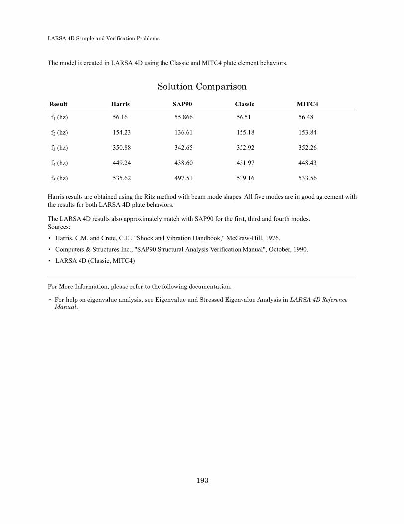
LARSA 4D Sample and Verification Problems
The model is created in LARSA 4D using the Classic and MITC4 plate element behaviors.
Solution Comparison
Result Harris SAP90 Classic MITC4
f1 (hz) 56.16 55.866 56.51 56.48
f2 (hz) 154.23 136.61 155.18 153.84
f3 (hz) 350.88 342.65 352.92 352.26
f4 (hz) 449.24 438.60 451.97 448.43
f5 (hz) 535.62 497.51 539.16 533.56
Harris results are obtained using the Ritz method with beam mode shapes. All five modes are in good agreement withthe results for both LARSA 4D plate behaviors.
The LARSA 4D results also approximately match with SAP90 for the first, third and fourth modes.Sources:
• Harris, C.M. and Crete, C.E., "Shock and Vibration Handbook," McGraw-Hill, 1976.
• Computers & Structures Inc., "SAP90 Structural Analysis Verification Manual", October, 1990.
• LARSA 4D (Classic, MITC4)
For More Information, please refer to the following documentation.
• For help on eigenvalue analysis, see Eigenvalue and Stressed Eigenvalue Analysis in LARSA 4D ReferenceManual.
193

LARSA 4D Sample and Verification Problems
194

LARSA 4D Sample and Verification Problems
E03: Beam Eigenvalues
A simply supported beam is subjected to its own weight. The span length is 80 inches and the beam is steel with 2 inchessquare cross section. The mass density of the beam is 0.000728 lb-sec2/in4. Determine the fundamental frequencyof the beam.
Example Project: The example described here can be found in the Eigenvalue folder of your LARSA 4D Samplesdirectory (generally My Documents\LARSA Projects\Samples) in the file E03.
Sample 16
The model of the beam has 5 joints and 4 beam elements. Joints 1 and 5 are pin supports. The joints 2, 3 and 4 representthe lateral dynamic degrees of freedom.
Modulus of Elasticity = 30,000,000 psi
Span Length = 80 inches
A = 4 in2
Izz = 1.3333 in4
Weight Density = 0.281 lb/in2 g = 386 in/sec2
Solution ComparisonSources:
• LARSA 4D
• Thomson, W.T., "Vibration Theory and Application," Prentice-Hall, Inc., Englewood Cliffs, N.Y., 2nd Printing,1965, p.18.
195

LARSA 4D Sample and Verification Problems
• Swanson Analysis Systems, Inc., "ANSYS Verification Manual".LARSA Thomson Swanson
f1 (Hertz) 28.77 28.77 28.77
For More Information, please refer to the following documentation.
• For help on eigenvalue analysis, see Eigenvalue and Stressed Eigenvalue Analysis in LARSA 4D ReferenceManual.
196
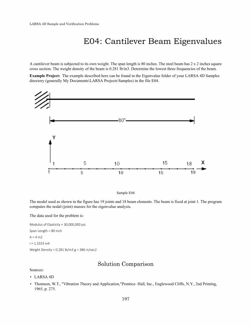
LARSA 4D Sample and Verification Problems
E04: Cantilever Beam Eigenvalues
A cantilever beam is subjected to its own weight. The span length is 80 inches. The steel beam has 2 x 2 inches squarecross section. The weight density of the beam is 0.281 lb/in3. Determine the lowest three frequencies of the beam.
Example Project: The example described here can be found in the Eigenvalue folder of your LARSA 4D Samplesdirectory (generally My Documents\LARSA Projects\Samples) in the file E04.
Sample E04
The model used as shown in the figure has 19 joints and 18 beam elements. The beam is fixed at joint 1. The programcomputes the nodal (joint) masses for the eigenvalue analysis.
The data used for the problem is:
Modulus of Elasticity = 30,000,000 psi
Span Length = 80 inch
A = 4 in2
I = 1.3333 in4
Weight Density = 0.281 lb/in3 g = 386 in/sec2
Solution ComparisonSources:
• LARSA 4D
• Thomson, W.T., "Vibration Theory and Application,"Prentice- Hall, Inc., Englewood Cliffs, N.Y., 2nd Printing,1965, p. 275.
197
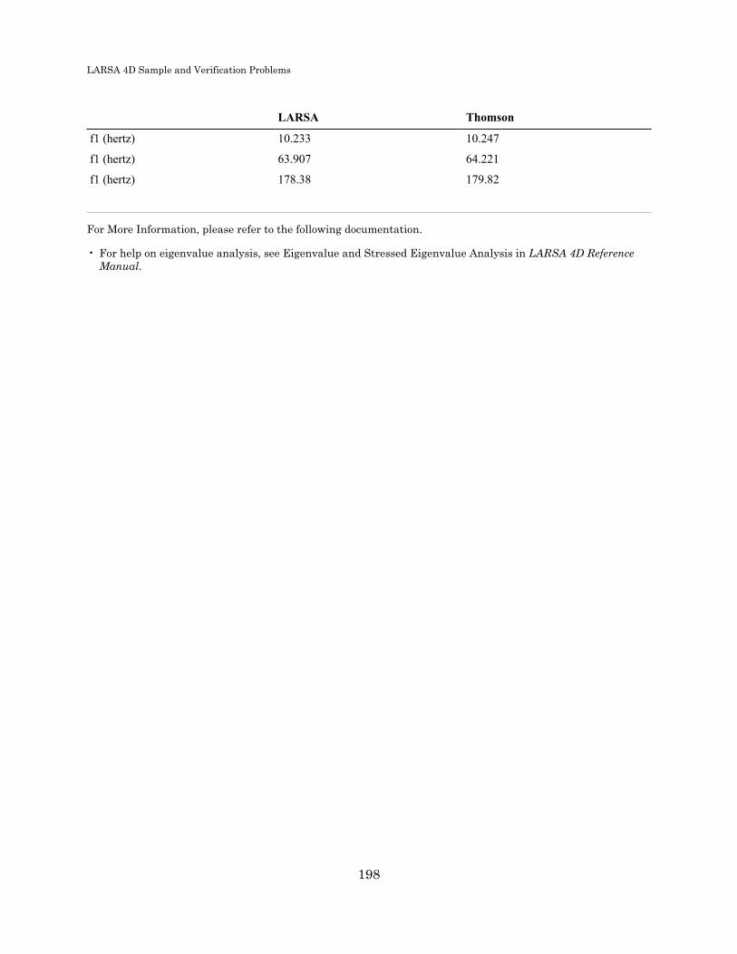
LARSA 4D Sample and Verification Problems
LARSA Thomson
f1 (hertz) 10.233 10.247
f1 (hertz) 63.907 64.221
f1 (hertz) 178.38 179.82
For More Information, please refer to the following documentation.
• For help on eigenvalue analysis, see Eigenvalue and Stressed Eigenvalue Analysis in LARSA 4D ReferenceManual.
198

LARSA 4D Sample and Verification Problems
E05: Rectangular Cantilever PlateEigenvalues
A rectangular cantilever plate of uniform thickness has its own weight as the sole loading. The plate is 16 inches inspan and 1 inch thick. The weight density of the plate is 0.281 lb/in3. The width of the plate is 4 inches. One four inchwide end of the plate is fixed. Determine the fundamental natural frequency.
Example Project: The example described here can be found in the Eigenvalue folder of your LARSA 4D Samplesdirectory (generally My Documents\LARSA Projects\Samples) in the file E05.
199

LARSA 4D Sample and Verification Problems
Sample E05
This is a rectangular plate with one edge fixed. The model used has 4 x 2 mesh size and consists of 15 joints and 8plate elements.
Modulus of Elasticity = 30,000,000 psi
Poisson's Ratio = 0.30
Shear Modulus = 11,538,461 psi
Weight Density = 0.281 lb/in3
Plate Thickness = 1 inch
Plate Width = 4 inches
Span Length = 16 inches g = 386.4 in/sec2
200

LARSA 4D Sample and Verification Problems
The model is created in LARSA 4D using the Classic and MITC4 plate element behaviors.
Solution Comparison
Result Timoshenko Classic MITC4
f1 128.09 128.11 128.11
Sources:
• Timoshenko, S., and Young,D.H., "Vibration Problems in Engineering 7quot;, 3rd Edition, D. Van NostrandCo.,Inc., New York, 1955, p. 389.
• LARSA 4D (Classic, MITC4)
For More Information, please refer to the following documentation.
• For help on eigenvalue analysis, see Eigenvalue and Stressed Eigenvalue Analysis in LARSA 4D ReferenceManual.
201

LARSA 4D Sample and Verification Problems
202

LARSA 4D Sample and Verification Problems
E06: Mass Spring ModelEigenvalues
This is a system with two lumped masses and three springs. Determine the fundamental natural frequency.
Example Project: The example described here can be found in the Eigenvalue folder of your LARSA 4D Samplesdirectory (generally My Documents\LARSA Projects\Samples) in the file E06.
203

LARSA 4D Sample and Verification Problems
Sample E06
The model has 4 joints, 3 spring elements and 2 joint masses. The dynamic degrees of freedom is selected in the GlobalX-direction so that it matches with the spring directions.
The joint locations in the X direction are arbitrarily selected since the length has no effect on the stiffness of a springelement. The translational degrees of freedom in X direction at joints 2 and 3 are the degrees of freedom of the model.All other degrees of freedom are eliminated from the model. The values for the lumped masses and spring constantsare given as:
M1= 0.5 lb-sec2/in
M2 = 1.0 lb-sec2/in
204

LARSA 4D Sample and Verification Problems
K1 = 200 lb/in
K2 = 800 lb/in
K3 = 200 lb/in
Solution ComparisonSources:
• Thomson, W.T.,"Vibration Theory and Applications," Prentice- Hall, Inc., Englewood Cliffs, N.Y., 2nd Edition,1965, P. 163.
• LARSA 4DThomson LARSA
f1 (hz) 2.5814 2.5814
f1 (hz) 8.3263 8.3263
For More Information, please refer to the following documentation.
• For help on eigenvalue analysis, see Eigenvalue and Stressed Eigenvalue Analysis in LARSA 4D ReferenceManual.
205

LARSA 4D Sample and Verification Problems
206

LARSA 4D Sample and Verification Problems
E07: 2D Frame (Wilson & Bathe)Eigenvalues
This 2D frame structure has 10 equal bays and 9 stories. The bottom ends of the base columns are fixed. All membershave the same section properties. Determine the frame's three lowest natural frequencies.
Example Project: The example described here can be found in the Eigenvalue folder of your LARSA 4D Samplesdirectory (generally My Documents\LARSA Projects\Samples) in the file E07.
Sample E07
The material properties of the beams and columns are:
Modulus of Elasticity = 432,000 kip/ft2
Weight Density = 1 kip/ft3
The sectional properties of the beams and columns are:A = 3.00 ft2
Izz = 1.00 ft4
The geometry of the structure is based on:Column Height = 10 feet
Column Spacing = 20 feet
The frame is modeled in the global XZ plane with Z as the vertical direction. The joints are numbered such that thefooting level is 1 to 11. First level joints are from 101-111, second level joints are from 201-211, etc. The joints along
207

LARSA 4D Sample and Verification Problems
the base are completely fixed. Columns are numbered 1 to 99 from bottom to top and left to right. The beams arenumbered 100-189. The local z-axis of all beams and columns is normal to the plane of the frame.
This is a plane (2D) model, the degrees of freedom for the out-ofplane translational displacement (in Y) and in-planerotations (about X and Z) are removed from the analysis. The joints can move in Global X and Z directions and rotateabout the Global Yaxis.
Solution ComparisonSources:
• LARSA 4D
• Bathe,K.J., Wilson,E.L., "Large Eigenvalue Problems in Dynamic Analysis", Journal of the Eng.Mech.Div.,ASCE, Vol.98, No. EM6, Proc.Paper 9433, Dec 1972.
• Computers & Structures Inc., "SAP90 Structural Analysis Verification Manual", October 1990, 2-1.LARSA Bathe SAP90
f1 (hertz) 0.122202 0.122202 0.122202
f2 (hertz) 0.374165 0.374165 0.374165
f3 (hertz) 0.648210 0.648210 0.648210
The comparison of the frequencies for all three modes are good between LARSA and the references.
References• Ref [3] - Peterson, F.E., "EASE2, Elastic Analysis of Structural Engineering, Example Problem Manual,"
Engineering Analysis Corporation, Berkeley, California, 1981.
For More Information, please refer to the following documentation.
• For help on eigenvalue analysis, see Eigenvalue and Stressed Eigenvalue Analysis in LARSA 4D ReferenceManual.
208

LARSA 4D Sample and Verification Problems
E08: ASME Frame Eigenvalues
This frame is from ASME 1972 Program Verification and Qualification Library. It is a single story 3D frame with asingle bay in each direction. The frame is made of 2-inch steel pipe segments welded to 2.75-inch steel cubes. Thelegs are welded to a heavy base plate to assure full restraint.
Example Project: The example described here can be found in the Eigenvalue folder of your LARSA 4D Samplesdirectory (generally My Documents\LARSA Projects\Samples) in the file E08.
Determine the lowest 24 natural frequencies and mode shapes of the 3D structure considering the shear deformations.
Sample 31
The material properties of the pipes are:
Modulus of Elasticity = 27,900,000 lb/in2
Poisson's Ratio = 0.30
209

LARSA 4D Sample and Verification Problems
Shear Modulus = 10,730,769 lb/in2
The pipe section is constant throughout with 2.375 in. outer diameter and 0.154 in. wall thickness. The sectionproperties for the pipes are:Axx = 1.0745 in2
Ayy = 0.5037 in2
Azz = 0.5037 in2
Ixx = 1.3314 in4
Iyy = 0.6657 in4
Izz = 0.6657 in4
The self weight of the structure is represented by mass elements at the joints. The steel cubes are modeled as masselements at the corner joints of the frame.
The mass elements at the corner joints including the weight of 2.75 inch steel cubes are:Mxt = 0.0253816 lb-sec2/in
Myt = 0.0253816 lb-sec2/in
Mzt = 0.0253816 lb-sec2/in
The mass elements at all other joints are specified as:Mxt = 0.00894223 lb-sec2/in
Myt = 0.00894223 lb-sec2/in
Mzt = 0.00894223 lb-sec2/in
Solution ComparisonNatural Frequencies (Hertz)Sources:
• ANSYS, Engineering Analysis System, Examples Manual, Swanson Analysis Systems, Inc., Elizabeth, PA, 1977.
• EASE2, Elastic Analysis for Structural Engineering, Example Problem Manual, Engineering AnalysisCorporation,
• COSMOS, Finite Element Analysis Program
• LARSA 4DANSYS EASE2 COSMOS LARSA
Mode 1 111.52 111.53 111.2 111.21
Mode 2 115.95 115.96 115.8 115.77
Mode 3 137.60 137.61 137.1 137.13
Mode 4 218.02 218.03 215.7 215.74
Mode 5 404.23 404.23 404.1 404.16
Mode 6 422.70 422.72 422.50
Mode 7 451.72 451.75 451.45
Mode 8 553.99 554.07 548.80
Mode 9 735.70 735.81 733.29
210

LARSA 4D Sample and Verification Problems
ANSYS EASE2 COSMOS LARSA
Mode 10 762.32 762.44 758.26
Mode 11 852.57 852.72 850.98
Mode 12 894.08 894.26 891.85
The natural frequencies computed by LARSA are in good agreement with the values obtained by ANSYS and EASE2programs. LARSA and COSMOS results are identical. In ANSYS and EASE2 solutions, 24 eigenvalues are computedusing the Guyan reduction method retaining only 24 mass degrees of freedom, whereas in LARSA and COSMOS, theeigenvalue problem has been solved using all degrees of freedom.
References• Program Verification and Qualification Library, ASME Pressure Vessel and Piping Division, Committee on
Computer Technology, 1972.
For More Information, please refer to the following documentation.
• For help on eigenvalue analysis, see Eigenvalue and Stressed Eigenvalue Analysis in LARSA 4D ReferenceManual.
211

LARSA 4D Sample and Verification Problems
212

LARSA 4D Sample and Verification Problems
E09: Natural Frequencies of aTorsional System
A simple torsional system has two torsional springs with stiffness K = 100.0 lb-in/rad and two mass elements withrotary inertia of 1.0 lb-in-sec2. Determine the lowest two natural frequencies and mode shapes of the system.
Example Project: The example described here can be found in the Eigenvalue folder of your LARSA 4D Samplesdirectory (generally My Documents\LARSA Projects\Samples) in the file E09.
Sample E09
The system is modeled using 2-node torsional spring elements and mass elements. Joint 1 is fixed and all degrees offreedom except rotation about the Global X are restrained at joints 2 and 3.
Solution ComparisonNatural Frequencies (rad/sec)Sources:
• W.T. Thomson, "Theory of Vibration with Applications", Prentice-Hall Inc., Englewood Cliffs, NJ, 2nd Edition(1981).
• EMRC, "NISA II Verification Problems Manual", 1991.
• LARSA 4DThomson EMRC LARSA
Mode 1 f=0.9836 (hertz) 6.18 6.18 6.18
Mode 2 f=2.5752 (hertz) 16.18 16.18 16.18
For More Information, please refer to the following documentation.
• For help on eigenvalue analysis, see Eigenvalue and Stressed Eigenvalue Analysis in LARSA 4D ReferenceManual.
213

LARSA 4D Sample and Verification Problems
214

LARSA 4D Sample and Verification Problems
Samples for StressedEigenvalue Analysis
These samples provide an overview of the stressed eigenvalue analysis.
For More Information, please refer to the following documentation.
• For help on stressed eigenvalue analysis, see Eigenvalue and Stressed Eigenvalue Analysis in LARSA 4DReference Manual.
ES01: Vibrations of Axially Loaded Beam - Nonlinear 217Solution Comparison 218
215

LARSA 4D Sample and Verification Problems
216

LARSA 4D Sample and Verification Problems
ES01: Vibrations of Axially LoadedBeam - Nonlinear
A beam is subjected to the action of self-weight and an axial compressive force P. The beam is 80 inches long andpinned at both ends. The magnitude of the axial compressive load is 40,000 lbs. The weight of the beam is consideredand the weight density is 0.281 lb/in3. The beam has a square cross-section of 2 x 2 inches.
Example Project: The example described here can be found in the Stressed Eigenvalue folder of your LARSA 4DSamples directory (generally My Documents\LARSA Projects\Samples) in the file ES01.
Determine the axial deflection and maximum stress under static loading. Use the results to determine the first threenatural frequencies of the structure and the slope at the left-hand support. Eigenvalue analysis uses the stiffness matrixof the deformed and stressed structure.
Sample ES01
The model is selected with enough elements to characterize the dynamic behavior.
Modulus of Elasticity = 30,000,000 lb/in2
Span Length = 80 inches
A = 4 in2
I = 1.3333 in4
Weight Density = 0.281 lb/in3
Axial Load = 40,000 lb (compression)
The axial load is applied at joint 14 in the negative X direction.
217
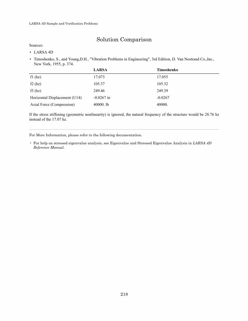
LARSA 4D Sample and Verification Problems
Solution ComparisonSources:
• LARSA 4D
• Timoshenko, S., and Young,D.H., "Vibration Problems in Engineering", 3rd Edition, D. Van Nostrand Co.,Inc.,New York, 1955, p. 374.
LARSA Timoshenko
f1 (hz) 17.073 17.055
f2 (hz) 105.37 105.32
f3 (hz) 249.46 249.39
Horizontal Displacement (U14) -0.0267 in -0.0267
Axial Force (Compression) 40000. lb 40000.
If the stress stiffening (geometric nonlinearity) is ignored, the natural frequency of the structure would be 28.76 hzinstead of the 17.07 hz.
For More Information, please refer to the following documentation.
• For help on stressed eigenvalue analysis, see Eigenvalue and Stressed Eigenvalue Analysis in LARSA 4DReference Manual.
218

LARSA 4D Sample and Verification Problems
Samples for Response SpectraAnalysis
These samples provide an overview of the response spectra analysis.
For More Information, please refer to the following documentation.
• For help on response spectra analysis, see Response Spectra Analysis in LARSA 4D Reference Manual.
RSA01: 2D Frame with Static and Seismic Loads 221Solution Comparison 224References 227
219

LARSA 4D Sample and Verification Problems
220

LARSA 4D Sample and Verification Problems
RSA01: 2D Frame with Static andSeismic Loads
A seven-story 2D frame structure is subjected to static lateral loads, static vertical loads and dynamic (seismic) lateralloads. The dynamic loads are represented by a response spectrum. The analysis is performed for two independentstatic load cases and one dynamic load case. Load combinations are generated to combine the static load cases withthe dynamic load condition.
Example Project: The example described here can be found in the Response Spectra folder of your LARSA 4DSamples directory (generally My Documents\LARSA Projects\Samples) in the file RSA01.
Sample RSA01
221

LARSA 4D Sample and Verification Problems
Determine the displacements and element forces for all static and dynamic load conditions. Also, determine the modeshapes and natural frequencies of the structure.
The 2-D model consists of 24 joints and 35 beam elements. This is plane frame problem. The translational displacementin Global Z-direction and rotations about Global X and Y-directions are deleted from the model. The joints 1, 2 and3 are fixed supports.
The material property data is given:
Modulus of Elasticity = 29,500 ksi
and sectional property data:Area = 51.17 in2 Izz = 2150 in4 Designation = S1
Area = 62.10 in2 Izz = 2670 in4 Designation = S2
Area = 72.30 in2 Izz = 3230 in4 Designation = S3
Area = 84.40 in2 Izz = 3910 in4 Designation = S4
Area = 50.00 in2 Izz = 3330 in4 Designation = S5
Area = 50.00 in2 Izz = 4020 in4 Designation = S6
Area = 50.00 in2 Izz = 5120 in4 Designation = S7
In the reference, to reduce the size of the system of equations, the lateral (X) displacements of the exterior columns havebeen constrained to the lateral (X) displacements of the middle column at each corresponding level. This eliminates allaxial deformations in the beams. A DOF Constraint is used to produce a model similar to Ref [2] for the comparisonof the results.
The primary load cases are defined as:
LoadCase Type Load Case Definition
1 STATIC STATIC VERTICAL LOADS
2 STATIC STATIC LATERAL LOADS
3 RSA LATERAL DYNAMIC LOADS
The combined (factored) load cases are:
Comb Case (Primary Load Case x Contribution Factor)
1 (Case 1 x 1.00) + (Case 2 x 1.00)
2 (Case 1 x 1.00) + (Case 3 x 1.00)
3 (Case 1 x 1.00) + (Case 3 x -1.00)
The load combination 1 combines the static vertical and lateral loads. The load combination 2 combines the staticvertical load condition with the dynamic load condition. The load combination case 3 combines the static vertical loadcase with the dynamic load case with the signs reversed.
Load Case 1 (Static Vertical Loads):
The static vertical load is applied on all horizontal beam elements 22 to 35 and it consists of:
Uniform Load W = 0.1 kip/ft (0.008333 kip/in)
Point Load P = 20 kips @ 10 ft from the I-end of the beam
222
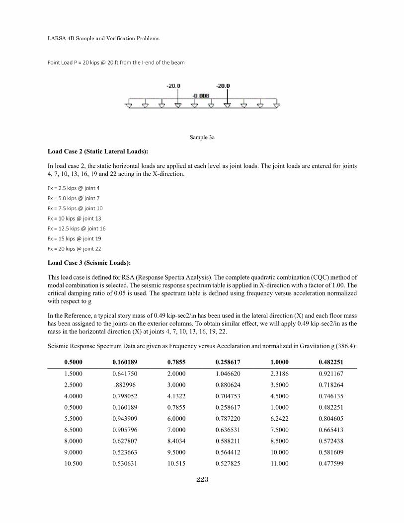
LARSA 4D Sample and Verification Problems
Point Load P = 20 kips @ 20 ft from the I-end of the beam
Sample 3a
Load Case 2 (Static Lateral Loads):
In load case 2, the static horizontal loads are applied at each level as joint loads. The joint loads are entered for joints4, 7, 10, 13, 16, 19 and 22 acting in the X-direction.
Fx = 2.5 kips @ joint 4
Fx = 5.0 kips @ joint 7
Fx = 7.5 kips @ joint 10
Fx = 10 kips @ joint 13
Fx = 12.5 kips @ joint 16
Fx = 15 kips @ joint 19
Fx = 20 kips @ joint 22
Load Case 3 (Seismic Loads):
This load case is defined for RSA (Response Spectra Analysis). The complete quadratic combination (CQC) method ofmodal combination is selected. The seismic response spectrum table is applied in X-direction with a factor of 1.00. Thecritical damping ratio of 0.05 is used. The spectrum table is defined using frequency versus acceleration normalizedwith respect to g
In the Reference, a typical story mass of 0.49 kip-sec2/in has been used in the lateral direction (X) and each floor masshas been assigned to the joints on the exterior columns. To obtain similar effect, we will apply 0.49 kip-sec2/in as themass in the horizontal direction (X) at joints 4, 7, 10, 13, 16, 19, 22.
Seismic Response Spectrum Data are given as Frequency versus Accelaration and normalized in Gravitation g (386.4):
0.5000 0.160189 0.7855 0.258617 1.0000 0.482251
1.5000 0.641750 2.0000 1.046620 2.3186 0.921167
2.5000 .882996 3.0000 0.880624 3.5000 0.718264
4.0000 0.798052 4.1322 0.704753 4.5000 0.746135
0.5000 0.160189 0.7855 0.258617 1.0000 0.482251
5.5000 0.943909 6.0000 0.787220 6.2422 0.804605
6.5000 0.905796 7.0000 0.636531 7.5000 0.665413
8.0000 0.627807 8.4034 0.588211 8.5000 0.572438
9.0000 0.523663 9.5000 0.564412 10.000 0.581609
10.500 0.530631 10.515 0.527825 11.000 0.477599
223

LARSA 4D Sample and Verification Problems
11.500 0.493366 12.000 0.518093 12.500 0.520045
12.579 0.519598 13.000 0.505311
Procedure for Analysis:
First the analysis is performed for the static load cases using the Linear Static Analysis option of LARSA. For thestatic analysis, the program automatically considers only the static load cases.
The next step is to return to the preprocessor and request Unstressed Eigenvalue Analysis for 7 mode shapes. Youmust select Keep Previous Results option from the Run dialog box to keep the results from static analysis run.
After eigenvalue analysis, return to the preprocessor and request Response Spectra Analysis. The spectrum table forthis problem is provided in a file with filename RSATBL03. Use this file as the file for response spectrum data.
All the results from static, eigenvalue and response spectra analysis are in the postprocessor.
Solution ComparisonThe results for static, dynamic and for load combinations as computed in LARSA are identical to the results in theReference.
The sign for the participation and amplitude factors are different in LARSA and SAP90 because of using a differentplane of analysis. However, keeping the sign is important for CQC method of modal combination to obtain correctresults.
The modal amplitude factors and spectral accelerations, velocities and displacements, CQC modal correlation factorsare tabulated in the LARSA output file with extension LI3.Sources:
• "SAP90, A Series of Computer Programs for the Finite Element Analysis of Structures. Verification Manual",Computers & Structures, 1992.
• LARSA 4DSAP90 LARSA
Static Analysis Results (Load Case2)
X Disp @ Joint 22 (inch) 1.079 1.450764
Axial Force - Member 1 (kip) 69.99 (Tension) -69.99
Moment - Member 1 (kip-in) 2324.68 2324.68
Eigenvalue Analysis Results
Frequency = f1 (hz) 0.7854 0.7854
Frequency = f2 (hz) 2.3187 2.3187
Frequency =f3 (hz) 4.1315 4.1315
Frequency =f4 (hz) 6.2430 6.2430
Frequency =f5 (hz) 8.4041 8.4041
Frequency = f6 (hz) 10.519 10.519
Frequency = f7 (hz) 12.576 12.576
224

LARSA 4D Sample and Verification Problems
SAP90 LARSA
Participation Factors for X-Direction
Mode=1 Frequency=0.7854 1.66 -1.656
Mode=2 Frequency=2.3187 0.624 -0.624
Mode=3 Frequency=4.1315 -0.379 0.379
Mode=4 Frequency=6.2430 -0.269 0.269
Mode=5 Frequency=8.4041 0.220 -0.220
Mode=6 Frequency=10.519 0.153 -0.153
Mode=7 Frequency=12.576 0.103 0.103
Modal Amplitude Factors in X-Direction
Mode=1 Frequency=0.7554 6.7948 -6.7948
Mode=2 Frequency=2.3187 1.0457 -1.0457
Mode=3 Frequency=4.1315 -0.1532 0.1532
Mode=4 Frequency=6.2430 -0.0544 0.0544
Mode=5 Frequency=8.4041 0.01795 -0.01795
Mode=6 Frequency=10.519 0.007124 -0.007124
Mode=7 Frequency=12.576 0.003319 0.003319
Spectral Acceleration in X-Direction
Mode=1 Frequency=0.79 99.92 99.92
Mode=2 Frequency=2.32 355.93 355.93
Mode=3 Frequency=4.13 272.52 272.52
Mode=4 Frequency=6.24 311.02 311.02
Mode=5 Frequency=8.40 227.24 227.24
Mode=6 Frequency=10.52 203.79 203.79
Mode=7 Frequency=12.58 200.78 200.78
Velocity in X-Direction
Mode=1 Frequency=0.79 20.25 20.25
Mode=2 Frequency=2.32 24.43 24.43
Mode=3 Frequency=4.13 10.50 10.50
Mode=4 Frequency=6.24 7.93 7.93
Mode=5 Frequency=8.40 4.30 4.30
Mode=6 Frequency=10.52 3.08 3.08
Mode=7 Frequency=12.58 2.54 2.54
Displacement in X-Direction
Mode=1 Frequency=0.79 4.10 4.10
Mode=2 Frequency=2.32 1.68 1.68
225

LARSA 4D Sample and Verification Problems
SAP90 LARSA
Mode=3 Frequency=4.13 0.40 0.40
Mode=4 Frequency=6.24 0.20 0.20
Mode=5 Frequency=8.40 0.08 0.08
Mode=6 Frequency=10.52 0.05 0.05
Mode=7 Frequency=12.58 0.03 0.03
Displacements and Member Forces
Horizontal Displacement @ Joint 22 5.4313 5.4313
Axial Force in Member 1 261.5 261.5
Moment in Member 1 9916 9916
Load Combination HorizontalDisplacements
Joint=1 0.00000 0.00000
Joint=4 0.702191 0.702201
Joint=7 1.727692 1.727689
Joint=10 2.662273 2.662265
Joint=13 3.554482 3.554485
Joint=16 4.331373 4.331372
Joint=19 5.004939 5.004927
Joint=22 5.413500 5.431349
Load Combination VerticalDisplacements
Joint=1 0.00000 0.00000
Joint=4 0.008850 0.008853
Joint=7 0.015564 0.015570
Joint=10 0.019761 0.019769
Joint=13 0.022620 0.022630
Joint=16 0.023609 0.023621
Joint=19 0.023333 0.023346
Joint=22 0.022588 0.022602
Load Combination HorizontalReaction Forces
Joint=1 94.50 94.50
Joint=2 133.8 133.8
Joint=3 84.07 84.07
Load Combination Vertical ReactionForces
Joint=1 406.52 406.52
226

LARSA 4D Sample and Verification Problems
SAP90 LARSA
Joint=4 312.0 312.0
Joint=7 406.5 406.5
Load Combination Vertical ReactionMoments
Joint=1 9634.23 9434.23
Joint=4 13390 13394
Joint=7 10200 10197
Modal Correlation Factors in CQC:
Mode 1 2 3 4 5 6 7
1 1.00 0.01
2 0.01 1.00 0.03 0.01
3 0.03 1.00 0.05 0.02 0.01 0.01
4 0.01 0.05 1.00 0.10 0.03 0.02
5 0.02 0.10 1.00 0.16 0.06
6 0.01 0.03 0.16 1.00 0.24
7 0.01 0.02 0.06 0.24 1.00
References• "Static and Dynamic Analysis of Multistory Frame Structure Using DYNAMIC/EASE2," Engineering
Analysis Corporation and Computers/Structures International.
For More Information, please refer to the following documentation.
• For help on response spectra analysis, see Response Spectra Analysis in LARSA 4D Reference Manual.
227

LARSA 4D Sample and Verification Problems
228

LARSA 4D Sample and Verification Problems
Samples for Time HistoryAnalysis
These samples provide an overview of the linear and nonlinear time history analysis and the linear dynamic rollingstock analysis.
For More Information, please refer to the following documentation.
• For help on time history analysis, see Linear Time History Analysis in LARSA 4D Reference Manual.
TH01: Spring Mass System Time History Analysis 231Solution Comparison 232
TH02: Beam with Concentrated Mass & Dynamic Load 233Solution Comparison 234
TH03: Cantilever Beam Time History Analysis 237Solution Comparison 239References 240
TH04: Dynamic Analysis of a Bridge 241Solution Comparison 241
TH05: Two dimensional frame with linear viscous damper 243Background 243Example Problem 243Solution and Comparison 245Nonlinear Dashpots 246Limitations 248References 248
TH15: Rolling Stock Analysis 249Model Setup 249Rolling Stock Analysis 252Moving Load Analysis 254Comparison of Results 255Dynamic Effect 257
229

LARSA 4D Sample and Verification Problems
230

LARSA 4D Sample and Verification Problems
TH01: Spring Mass System TimeHistory Analysis
A spring is supporting concentrated mass and subjected to a dynamic load with a rise time and a maximum value.Determine the maximum deflection and time of maximum response.
Example Project: The example described here can be found in the Time History folder of your LARSA 4DSamples directory (generally My Documents\LARSA Projects\Samples) in the file TH01.
Sample TH01
231

LARSA 4D Sample and Verification Problems
The model consists of 2 joints, 1 spring element and 1 mass element. The joint locations are selected arbitrarily. Thestiffness of a spring element is defined as the force per unit displacement. The length of the spring has no effect on thesolution. The structural model has one degree of freedom in the direction of the spring where the mass is attached.
In LARSA 4D, mass is entered in force units. However, in this verification problem, mass is given in kips-sec2/in(a unit related to the slug). In order to convert it to force units, it should be multiplied by gravitational acceleration(386.0886 in/sec2).
The integration time step of 0.004 seconds is used with total of 40 time steps. The results are reported for all time steps.
M = 0.0259067 kips-sec2/in
g = 386.0886 in/sec2
M = 0.0259067 * 386.0886 = 10 kips
k = 83.4 kips/in
Force = 20 kips after 0.075 rise time
The time history database file for this problem is in a DTH file.
Solution ComparisonSources:
• Biggs, J.M., "Introduction to Structural Dynamics," McGraw-Hill Book Co., New York, 1964, p 50.
• Swanson Analysis Systems, Inc., "ANSYS Verification Manual".
• LARSA 4DBiggs Swanson LARSA
Displacement (in) 0.331 0.33440 0.3356
Time (sec) 0.096 0.096 0.096
For More Information, please refer to the following documentation.
• For help on time history analysis, see Linear Time History Analysis in LARSA 4D Reference Manual.
232
LARSA 4D Sample and Verification Problems
TH02: Beam with ConcentratedMass & Dynamic Load
A steel beam supporting a concentrated mass is subjected to a dynamic load with a rise time and a maximum value.The weight of the beam is considered negligible. The beam is 20 feet in span and the moment of inertia in the planeof bending is 800.6 in4. The rise time of the applied dynamic load (from zero to 20 kips) is 0.075 seconds and the loadon the beam stays as 20 kips after 0.075 seconds. Determine the maximum deflection, maximum bending moment(stress) and the time of the maximum response.
Example Project: The example described here can be found in the Time History folder of your LARSA 4DSamples directory (generally My Documents\LARSA Projects\Samples) in the file TH02.
The model consists of 3 joints, 2 beam elements and a lumped mass.
In LARSA 4D, mass is entered in force units. However, in this verification problem, mass is given in kips-sec2/in(a unit related to the slug). In order to convert it to force units, it should be multiplied by gravitational acceleration(386.0886 in/sec2).The integration time step chosen is 0.004 seconds.
Modulus of Elasticity = 30,000 ksi
Span = 20 feet Izz = 800.6 in4
Force = 20 kips with rise time of 0.075 seconds
Mass = 0.0259067 kips-sec2/in
g = 386.0886 in/sec2
M = 0.0259067 * 386.0886 = 10 kips
The time history database file for this problem is in a DTH file.
233

LARSA 4D Sample and Verification Problems
Sample TH02
Solution ComparisonSources:
• Biggs, J. M., "Introduction to Structural Dynamics," McGraw-Hill Book Co., New York, 1964, p 50.
• Swanson Analysis Systems Inc., "ANSYS Verification Manual"
• LARSA 4DBiggs Swanson LARSA
Displacement (in) 0.331 0.33442 0.336
Time (sec) 0.096 0.096 0.096
Moment (kip-in) -1654 -1673 -1679
234

LARSA 4D Sample and Verification Problems
For More Information, please refer to the following documentation.
• For help on time history analysis, see Linear Time History Analysis in LARSA 4D Reference Manual.
235

LARSA 4D Sample and Verification Problems
236

LARSA 4D Sample and Verification Problems
TH03: Cantilever Beam Time HistoryAnalysis
A vertical load P is applied instantaneously at time zero on the free end of a cantilever beam. The beam is initially atrest. The load stays constant after time zero. The structure has two lumped masses. The damping is considered to beproportional to the mass. The beam is 100 inches in span with moment of inertia of 4 in4.
Determine the vertical displacement at the tip and the mid point of the beam as function of time.
Example Project: The example described here can be found in the Time History folder of your LARSA 4DSamples directory (generally My Documents\LARSA Projects\Samples) in the file TH03.
237

LARSA 4D Sample and Verification Problems
Sample TH03
The response is calculated by direct integration of the equations of motion. The structure is idealized as a 3 joint and2 beam element model with 2 lumped masses. The damping is specified as Rayleigh damping:[C] = a [M] + b [K]
In this problem, the damping is given as mass proportional damping with;a = 0.6312465
b = 0.
238

LARSA 4D Sample and Verification Problems
The material and sectional properties of the beam are:
Modulus of Elasticity = 1,000,000 lb/in2
Shear Modulus = 500,000 lb/in2
Izz = 4 in4
g = 386 in/sec2
The nodal (joint) mass elements are specified in the global Ydirection:
M2 = 2 lb-sec2/in
M3 = 1 lb-sec2/in
The load P versus time is entered using the Time History tool:
t (sec) P (lb)
0.0000 0.0
0.0099 0.0
0.0100 100.0
100.00 100.0
These data are saved in a DTH file. The linear time history analysis option of LARSA is executed using 80 time stepswith an integration time step of 0.02 seconds. This time step is about 1/20th of the period of the second mode and theerrors in the predicted response by direct integration will be very small. LARSA uses Newmark integration.
Solution ComparisonVertical Displacement (in inches) at the Tip Joint 3Sources:
• EASE2
• Problems 1-95 The last column (theory) is computed manually. Since the model has only (2) degrees of freedomwith mass proportional damping, the computation is relatively simple.
• LARSA 4DEASE2 Theory LARSA
t=0.00 0.0000 0.0000 0.0000
t=0.08 0.2396 0.3059 0.2396
t=0.16 0.9970 1.1187 0.9972
t=0.24 2.1082 2.2640 2.1086
t=0.32 3.4787 3.6658 3.4793
t=0.40 5.1027 5.3245 5.1037
t=0.48 6.9252 7.1666 6.9266
t=0.56 8.7679 8.9956 8.7694
239

LARSA 4D Sample and Verification Problems
EASE2 Theory LARSA
t=0.64 10.4305 10.6215 10.4320
t=0.72 11.8260 11.9830 11.8275
t=0.80 12.9664 13.0979 12.9677
t=0.88 13.8333 13.9282 13.8344
t=0.96 14.3270 14.3614 14.3276
t=1.04 14.3654 14.3334 14.3654
t=1.12 13.9874 13.9106 13.9868
t=1.20 13.3135 13.2143 13.3123
The last column (theory) is computed manually. Since the model has only (2) degrees of freedom with massproportional damping, the computation is relatively simple.
The (2 x 2) system is solved for two eigenvalues. The eigenvector for each mode is computed by substituting theeigenvalue for that 1-96 LARSA Examples & Verification mode. The eigenvectors are then normalized with respectto mass. From the modal damping matrix (2 x 2), the damping ratio for each mode is calculated. Using the modalloading for each mode, the modal responses are computed. The actual displacements are calculated by superimposingthe responses contributed by each mode.
The results from LARSA and EASE2 are identical and they compare well to the response computed manually usingthe modal superposition.
References• Peterson, F.E., “EASE2 - Example Problem Manual”, 1981, Problem 3.02 & 4.02.
For More Information, please refer to the following documentation.
• For help on time history analysis, see Linear Time History Analysis in LARSA 4D Reference Manual.
240

LARSA 4D Sample and Verification Problems
TH04: Dynamic Analysis of a Bridge
A three-span reinforced-concrete bridge is subjected to the three-dimensional ground displacement records of the 1994Northridge earthquake.
Example Project: The example described here can be found in the Time History folder of your LARSA 4DSamples directory (generally My Documents\LARSA Projects\Samples) in the file TH04.
The structure is identical to the collapsed first frame of the SR14/15 southbound separation and overhead bridge located25 miles north of downtown Los Angeles. The ground motion is believed to have varied in space during actual eventdue to wave passage and loss of coherence effects, as well as different local soil conditions at the supports.
Determine the response of the structure to spatially varying support displacements by direct integration of the equationsof motion with a time step of DeltaT = 0.02sec.
Assume the analysis height of the piers to be equal to the distance from the grade level to the center of gravity of thedeck, and account for soil-structure interaction by using foundation springs. Use classical Rayleigh damping with 5%damping ratios for the first and fifth modes of vibration.
Sample TH04
Solution ComparisonSources:
• LARSA 4D
• ANSYS
• IDARCLARSA ANSYS IDARC
Natural Periods ofVibration
T1(sec) 1.002 1.002
T2(sec) 0.352 0.352
T3(sec) 0.217 0.217
T4(sec) 0.207 0.207
T5(sec) 0.197 0.197
241
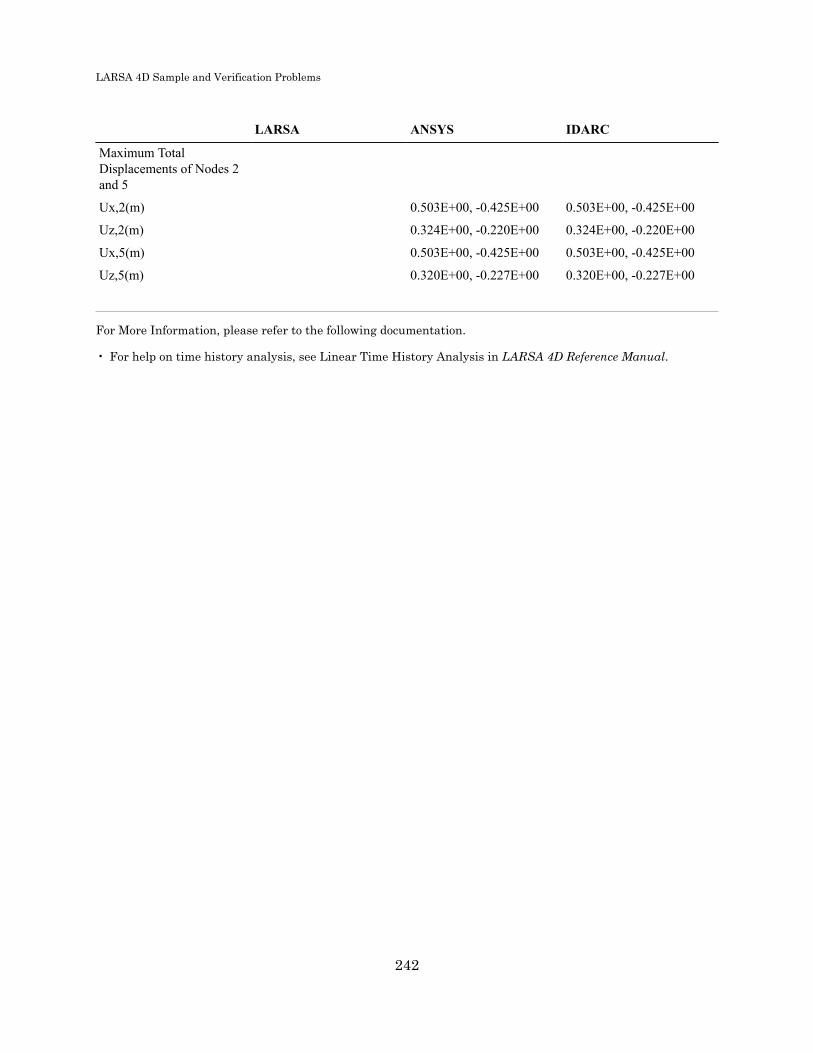
LARSA 4D Sample and Verification Problems
LARSA ANSYS IDARC
Maximum TotalDisplacements of Nodes 2and 5
Ux,2(m) 0.503E+00, -0.425E+00 0.503E+00, -0.425E+00
Uz,2(m) 0.324E+00, -0.220E+00 0.324E+00, -0.220E+00
Ux,5(m) 0.503E+00, -0.425E+00 0.503E+00, -0.425E+00
Uz,5(m) 0.320E+00, -0.227E+00 0.320E+00, -0.227E+00
For More Information, please refer to the following documentation.
• For help on time history analysis, see Linear Time History Analysis in LARSA 4D Reference Manual.
242

LARSA 4D Sample and Verification Problems
TH05: Two dimensional frame withlinear viscous damper
A two-dimensional three-story steel frame with linear viscous dampers at each story.
Example Project: The example described here can be found in the Time History folder of your LARSA 4DSamples directory (generally My Documents\LARSA Projects\Samples) in the file TH05N.
BackgroundViscous dashpot damping devices are widely used as structural protective systems for extreme loading (wind andearthquake) cases. Due to their combined benefits in terms of overall displacement reduction and energy dissipation,dampers are considered to be one of the most effective structural protective systems.
The dashpot isolator element in LARSA 4D is suitable for modeling the behavior of fluid viscous dampers or otherdevices displaying viscous behavior.
Fluid dampers which operate on the principle of fluid orificing, produce an output force which is proportional to apower of the velocity, i.e. Cvn, where C is a damping coefficient, v is the velocity across the dashpot, and n is an integerpower typically between 0.5 and 2.0 (1.0 implies linear behavior.)
Example ProblemIn this example a two dimensional three story experimental steel frame with linear viscous dashpots at each story, asshown in the figure below, is modeled in LARSA 4D. The dimensions and properties of the frame elements (fabricatedprimarily with ST 2X3.85 cut with depth = 1.5 inch) and mass assignments are adopted from Scheller and Constantinou(1997, 1999).
243

LARSA 4D Sample and Verification Problems
Three dimensional building (adapted from Scheller and Constantinou (1999) )
The member end offsets of the elements are modeled in order to simulate the stiffening effects of the floor weights(steel plates).
The dashpots have coefficient of damping as C = 160N-s/cm and velocity exponent (n) = 1. See below for a comparisonof linear (n=1) and nonlinear (n<1) dashpots.
The model is analyzed with the Nonlinear Time History Analysis in LARSA 4D with the S00E component of the ElCentro 1940 earthquake (pga = 0.343g).
Due to the diaphragm action in each floor, the building will typically have three modes. The periods of the buildingwithout the dampers, obtained from experiment and from LARSA 4D Eigenvalue analysis, are:
Mode Period (sec)
1 0.439
2 0.133
3 0.070
244

LARSA 4D Sample and Verification Problems
Solution and ComparisonSome representative displacement magnitudes of the 1st story of the frame from the LARSA analysis are:
time (sec) displacement (mm)
1 0.00
5 -0.28
10 0.48
The history of percent-normalized story drifts (100 x drift / story height), and the normalized story shear (sum ofcolumn shear divided by story weight) v/s normalized story drift obtained from LARSA 4D are compared with thecorresponding results from Scheller and Constantinou (1999):
Comparisons for the dynamic responses of the 2D frame
The comparisons indicate that the LARSA is capable of modeling linear dampers with appreciable accuracy.
245

LARSA 4D Sample and Verification Problems
Nonlinear DashpotsThis problem can also be run with a nonlinear dashpot, that is, with the velocity power n set to 0.75. The figure belowshows a comparison of story drifts for a linear (n=1) and nonlinear (n=0.75) dashpot.
246

LARSA 4D Sample and Verification Problems
Comparisons of story drifts for linear (n=1) and nonlinear (n=0.75) dampers
247

LARSA 4D Sample and Verification Problems
It should be noted that when the velocity exponent n is not 1.0, then the damping coefficient and velocity power mustbe chosen with respect to a particular choice of units. In the present example C is assumed to have unit as N-s/mm andv as mm/sec. Care should be taken for units of C and v when using nonlinear damping properties.
LimitationsLARSA 4D cannot model the traditional Maxwell or Kelvin elements with dashpots directly. However, those can bemodeled in LARSA 4D by combining the damping element with brace elements.
ReferencesScheller, J., and Constantinou, M. C. (1999). "Response History Analysis of Structures with Seismic Isolation andEnergy Dissipation Systems: Verification Examples for Program SAP2000." Technical Report MCEER-99-0002.University of Buffalo, State University of New York.
Seleemah, A A, and Constantinou, M C (1997). "Investigation of Seismic Response of Buildings with Linear andNonlinear Fluid Viscous Dampers." Technical Report NCEER-97-0004, SUNY, University at Buffalo.
For More Information, please refer to the following documentation.
• For help on time history analysis, see Linear Time History Analysis in LARSA 4D Reference Manual.
248

LARSA 4D Sample and Verification Problems
TH15: Rolling Stock Analysis
Rolling Stock Analysis is a linear Time History Analysis on moving load cases with load patterns and mass of thevehicle is not considered.
A single vehicle is moving on a simply supported bridge deck with a constant speed. Determine the mid-spandisplacements with respect to time and also the maximum bending moment when the vehicle is 140 ft away fromthe deck end.
Compare the Rolling Stock Analysis results with the ones of Moving Load Analysis that is linear elastic analysis onmoving load cases with load patterns.
Example Project: The example described here can be found in the TimeHistory folder of your LARSA 4DSamples directory (generally My Documents\LARSA Projects\Samples) in the file TH15.
Sample TH15
Model SetupA 600 ft long deck 700 inch wide is modeled with two different modeling approaches: girder with 60 beam elementsand girder as 60-by-1 plate mesh. The joints along the start of the decks are supported in all translation directions, andthe joints along the end of the deck are supported in y and z-translation. Both ends are also supported in x-rotation forthe model with beam elements (For plate model, no need to restrain rotation x).
249

LARSA 4D Sample and Verification Problems
Model View
A36 steel is assigned to the elements. Properties of A36 steel are:
E = 2.9E07 lb/in2
G = 1.12E07 lb/in2
Unit Weight = 0.2836 lb/in3
However, for the purposes of making a verification comparison to a static moving load analysis, set the unit weightof the material as small as 1.0E-05 lb/inch3 to remove the effect of the mass of the structure from the dynamic results.
A single lane whose width is 12 feet is defined on the deck surface. It is defined from Input Data → Geometry →Lanes/Surfaces . The path of the lane is defined along the deck and it is offset 180 inch from the center of the deckin the transverse direction.
250

LARSA 4D Sample and Verification Problems
Lane/Surface Geometry
Lane Path Definition
251

LARSA 4D Sample and Verification Problems
Surface Path Definition
In this example, "HS20-44" vehicle that exists in "movedata" database file, is moving on the defined lane/surfacefrom the start of the deck to its end with a velocity of 200.0 ft/sec. So connect the "movedata.dml" database to theproject.
Rolling Stock AnalysisIn this example, define two load cases, one is for the model with beams and the other for the model with plate elements.Select Time History for their Analysis Type although no time history load will be assigned.
Load Cases for Rolling Stock Analysis
Then, define moving loads from Moving Loads → Basic Moving Loads .
Select the lane that the load is moving on it and the vehicle, "HS20-44", as load pattern. Enter the vehicle speed as200 ft/sec.
252
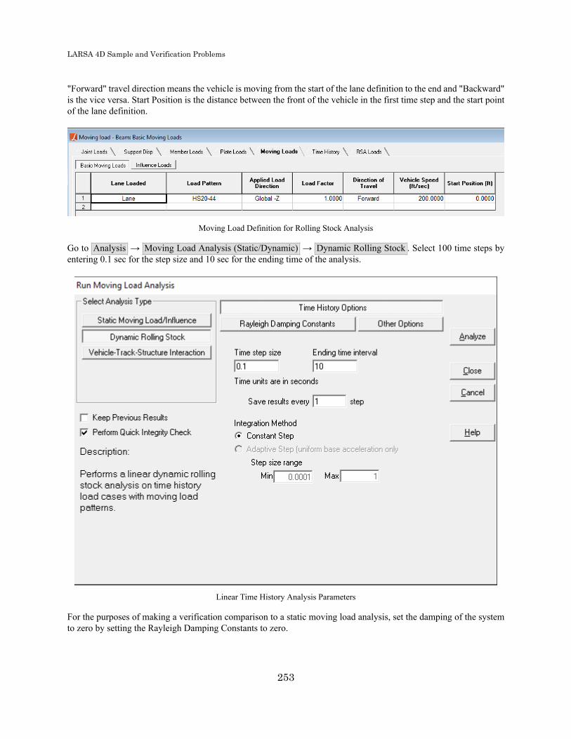
LARSA 4D Sample and Verification Problems
"Forward" travel direction means the vehicle is moving from the start of the lane definition to the end and "Backward"is the vice versa. Start Position is the distance between the front of the vehicle in the first time step and the start pointof the lane definition.
Moving Load Definition for Rolling Stock Analysis
Go to Analysis → Moving Load Analysis (Static/Dynamic) → Dynamic Rolling Stock . Select 100 time steps byentering 0.1 sec for the step size and 10 sec for the ending time of the analysis.
Linear Time History Analysis Parameters
For the purposes of making a verification comparison to a static moving load analysis, set the damping of the systemto zero by setting the Rayleigh Damping Constants to zero.
253

LARSA 4D Sample and Verification Problems
Rayleigh Damping Constants
Click Analyze to start the analysis.
Moving Load AnalysisThe same problem is solved by a Moving Load Analysis to verify the Rolling Stock Analysis results. Similarly, definetwo load cases for the beam and plate models but this time, Analysis Type should be set as Moving (Static) .
254

LARSA 4D Sample and Verification Problems
Load Cases for Moving Load Analysis
Define the moving load in a same way with the Rolling Stock Analysis. But this time, Position Increment shouldbe set instead of Vehicle Speed since it is a linear elastic analysis. By entering 20.0 feet to this parameter, vehicleposition will be identical for the both analyses' solution steps.
Moving Load Definition for Moving Load Analysis
Then, run Moving Load Analysis .
Comparison of ResultsDisplacement histories at mid-span (i.e. @300 feet) and maximum bending moments when the vehicle at 140 feet fromthe start of both beam and plate structures obtained from Rolling Stock Analysis (RoSA) and Moving Load Analysis(MovLoad) are compared to each other. Vehicle leaves the system at the end of 30th step in both Rolling Stock andMoving Load Analyses.
255

LARSA 4D Sample and Verification Problems
Mid-Span Displacements
Moment Diagrams when the Vehicle @ 140 ft
Max. Bending Moments on Deck when the Vehicle @ 140 ft (without Mass)
Model Max. Mz (kips-ft) Model Max. Mxx (kips-ft/ft)
MovLoad - Beam 6789.43 MovLoad - Plate 115.38
RoSA - Beam 6814.61 RoSA - Plate 115.47
256
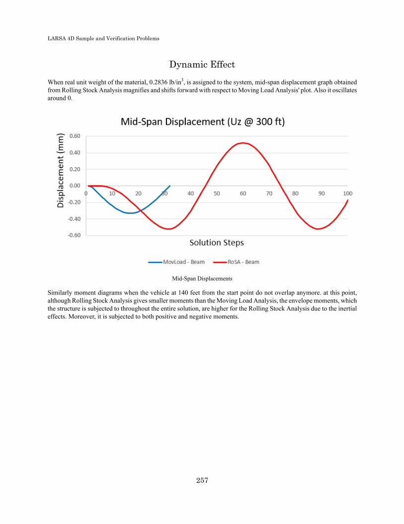
LARSA 4D Sample and Verification Problems
Dynamic Effect
When real unit weight of the material, 0.2836 lb/in3, is assigned to the system, mid-span displacement graph obtainedfrom Rolling Stock Analysis magnifies and shifts forward with respect to Moving Load Analysis' plot. Also it oscillatesaround 0.
Mid-Span Displacements
Similarly moment diagrams when the vehicle at 140 feet from the start point do not overlap anymore. at this point,although Rolling Stock Analysis gives smaller moments than the Moving Load Analysis, the envelope moments, whichthe structure is subjected to throughout the entire solution, are higher for the Rolling Stock Analysis due to the inertialeffects. Moreover, it is subjected to both positive and negative moments.
257
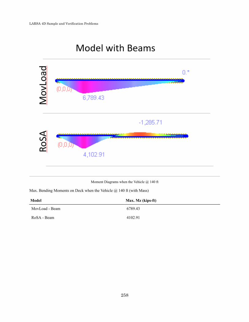
LARSA 4D Sample and Verification Problems
Moment Diagrams when the Vehicle @ 140 ft
Max. Bending Moments on Deck when the Vehicle @ 140 ft (with Mass)
Model Max. Mz (kips-ft)
MovLoad - Beam 6789.43
RoSA - Beam 4102.91
258

LARSA 4D Sample and Verification Problems
Moment Diagrams (Envelope)
Envelope Bending Moments on Deck (with Mass)
Model Max. Mz (kips-ft) Min. Mz (kips-ft)
MovLoad - Beam 10,519.01 0.0
RoSA - Beam 14,493.90 -13,984.54
For More Information, please refer to the following documentation.
• For help on rolling stock analysis, see Moving Load Analysis in LARSA 4D Reference Manual.• For help on time history analysis, see Linear Time History Analysis in LARSA 4D Reference Manual.
259

LARSA 4D Sample and Verification Problems
260

LARSA 4D Sample and Verification Problems
Samples for StagedConstruction Analysis
These samples provide an overview of staged construction analysis.
S01: Creep Effects - Simple Span Concrete Beam 263
S02: Creep and Shrinkage - Cantilevers Loaded at Different Times 265
S03: Creep and Shrinkage - Use CEB-FIP model code 1990 in S02 267
S04: Creep and Shrinkage - Connect Aging Cantilevers 269
S05: Creep and Shrinkage - Use CEB-FIP model code 1990 insample S04
271
S06: 3-Span Post-Tension Deck 273
S07: Composite I-Girder with Time-Dependent Effects 279Cross-Section Definition 279Model Geometry 279Construction Sequence 279Verification of Cross-Section Properties 280Verification of Self-Weight Loading 280Verification of the Time Effect on Elastic Modulus 282Verification of Shrinkage 283
S08: Time-Dependent Material Properties Effects 285Problem Definition 285Modeling 286Construction Sequence 289Verification of Creep 289Verification of Shrinkage 293
S08b: Time-Dependent Material Properties Effects 299Problem Definition 299Modeling 300Construction Sequence 305Verification of Creep 305Verification of Shrinkage 307
S09: Plates with Time-Dependent Material Effects 311Problem Definition 311
261

LARSA 4D Sample and Verification Problems
Modeling 312Verification of Creep 314Verification of Shrinkage 314Verification of Elastic Modulus Change 315
S09b: Plates with Time-Dependent Material Effects (OrthotropicMaterial)
317
Problem Definition 317Modeling 318Verification of Creep 319Verification of Shrinkage 320Verification of Elastic Modulus Change 320
262

LARSA 4D Sample and Verification Problems
S01: Creep Effects - Simple SpanConcrete Beam
This sample problem demonstrates how to model time-dependent creep effect for a simple span concrete beam.
Example Project: The example described here can be found in the Staged Construction folder of your LARSA 4DSamples directory (generally My Documents\LARSA Projects\Samples) in the file S01.
The formwork supporting wet concrete is removed 10 days after pouring the concrete. On day 50, beam is subjectedto additional superimposed load. The stage analysis can be summarized as:
CONSTRUCTION SCHEDULE
Concrete Cast at Day = 0
Remove Forms at Day = 10
Add Superimposed Dead Load at Day = 50
The model has 11 joints and 10 beam elements. Compute maximum vertical deflection and compare the results tothose by hand-calculations and by BD2 program.
Modulus of Elasticity = 661,305 lb/ft2
Span = 100 feet
A = 12.0 ft2
Izz = 36.0 ft4
Concrete fc28 = 6,500 psi
Relative Humidity = 70%
Temperature = 64 Fahrenheit
Time dependent stage analysis is performed using 11 construction stages and steps and maximum of 10 iterations willbe performed in each construction step.
263

LARSA 4D Sample and Verification Problems
264
LARSA 4D Sample and Verification Problems
S02: Creep and Shrinkage -Cantilevers Loaded at Different
Times
This problem involves 2 independent cantilevers, with loads applied at different times. One of the two cantilevers hastwo separate loads applied to it, but at different times. This sample demonstrates how different two cantilevers respondto time-dependent creep effect when loaded at different times.
Example Project: The example described here can be found in the Staged Construction folder of your LARSA 4DSamples directory (generally My Documents\LARSA Projects\Samples) in the file S02.
Use CEB-FIP model code 1978 with user-defined time dependent material curves in this sample.
CONSTRUCTION SCHEDULE
Concrete Cast at Day = 0
Remove Forms at Day = 28
Apply Load only to Left Cantilever at Day = 28
Apply Additional Loads to both Cantilevers at Day = 100
The model has 22 joints and 20 beam elements. Compare the results to those by hand-calculations and BC program.
Time dependent stage analysis is performed for all construction stages and maximum of 10 iterations is performedin each construction step.
265

LARSA 4D Sample and Verification Problems
266

LARSA 4D Sample and Verification Problems
S03: Creep and Shrinkage - UseCEB-FIP model code 1990 in S02
This problem involves 2 independent cantilevers, with loads applied at different times. One of the two cantilevers hastwo separate loads applied to it, but at different times. This sample demonstrates how different two cantilevers respondto time-dependent creep effect when loaded at different times.
Example Project: The example described here can be found in the Staged Construction folder of your LARSA 4DSamples directory (generally My Documents\LARSA Projects\Samples) in the file S03.
Use CEB-FIP model code 1990 with user-defined time dependent material curves in this sample.
CONSTRUCTION SCHEDULE
Concrete Cast at Day = 0
Remove Forms at Day = 28
Apply Load only to Left Cantilever at Day = 28
Apply Additional Loads to both Cantilevers at Day = 100
The model has 22 joints and 20 beam elements. Compare the results to those by hand-calculations and BC program.
Time dependent stage analysis is performed for all construction stages and maximum of 10 iterations is performedin each construction step.
267

LARSA 4D Sample and Verification Problems
268

LARSA 4D Sample and Verification Problems
S04: Creep and Shrinkage - ConnectAging Cantilevers
This is a simple stage analysis. The 2 cantilevers are first assembled at day 28 and allowed to age to day 50. At thatpoint, they are made fully connected at the free ends and allowed to age to day 4000. This sample allows us to see howinternal forces related to creep displacements are developing over time.
Example Project: The example described here can be found in the Staged Construction folder of your LARSA 4DSamples directory (generally My Documents\LARSA Projects\Samples) in the file S04.
Use CEB-FIP model code 1978 with user-defined time dependent material curves in this sample.
Time dependent stage analysis is performed for all construction stages using maximum of 10 iterations for constructionstage.
269

LARSA 4D Sample and Verification Problems
270
LARSA 4D Sample and Verification Problems
S05: Creep and Shrinkage - UseCEB-FIP model code 1990 in sample
S04
This is a simple staged construction analysis. The 2 cantilevers are first assembled at day 28 and allowed to age to day50. At that point, they are made fully connected at the free ends and allowed to age to day 4000. This sample allowsus to see how internal forces related to creep displacements are developing over time.
Example Project: The example described here can be found in the Staged Construction folder of your LARSA 4DSamples directory (generally My Documents\LARSA Projects\Samples) in the file S05.
Use CEB-FIP model code 1990 in this sample.
Time dependent stage analysis is performed for all construction stages using maximum of 10 iterations for constructionstage.
271

LARSA 4D Sample and Verification Problems
272

LARSA 4D Sample and Verification Problems
S06: 3-Span Post-Tension Deck
This sample problem (courtesy of International Bridge Technologies, San Diego) is for time-dependent constructionanalysis for a transit crossing which has post-tension concrete deck supported by two concrete piers. The structure has3 spans and 2 concrete piers. Each span has 3 bottom tendons. There are also 2 top slab continuity tendons.
Example Project: The example described here can be found in the Staged Construction folder of your LARSA 4DSamples directory (generally My Documents\LARSA Projects\Samples) in the file S06.
Sample S06
The deck concrete properties are:
f'c = 6500 psi
Poisson ratio = 0.2
Mean T = 64 Farhenheit
Density = 0.155 kip/ft3
s = 0.25 ( see CEB FIP 2.1.6.1)
RH = 70% (relative humidity)
h = 0.762 ft (notional thickness)
bsc = 5 (shrinkage coeff, see ceb fip 90)
The pier concrete properties are:
f'c = 5000 psi
Poisson ratio = 0.2
Mean T = 64 Farhenheit
Density = 0.155 kip/ft3
s = 0.25 ( see CEB FIP 2.1.6.1)
RH = 70% (relative humidity)
273

LARSA 4D Sample and Verification Problems
h = 2.545 ft (notional thickness)
bsc = 5 (shrinkage coeff, see ceb fip 90)
The tendon properties are:
STRAND AREA = 0.00151
ANCHOR-SET = 0.03125
FRICTION = 0.25
WOBBLE = 0.0002
Tendon Layouts
Tendon layouts are defined using the bottom of segments as reference. In this example, we will be using severalreference points defined from the bottom of the reference segment : at 5.330 feet (1), at 0.500 ft (2), at 5.833 ft (3), at3.833 ft (4), at 4.330 (5), at 1.670 (6), at 3.000 ft (7), at 6.500 ft (8).
Span 1 Bottom Tendon Layouts (PI is for POINT OF INTERSECTION)TENDON ID 11
38 STRANDS
LEFT ANCHOR AT 1.208 FT FROM START OF SEGMENT 100 AND 5.330 FT OFFSET FROM BOTTOM
RIGHT ANCHOR AT 1.46 FT FROM END OF SEGMENT 114 and 5.833 FT OFFSET FROM BOTTOM
(PI) AT 7.25 FROM START OF SEGM 104 AND 5.833 FT OFFSET FROM BOTTOM WITH RADIUS 20 FT
(PI) AT 3.25 FROM START OF SEGM 109 AND 0.500 FT OFFSET FROM BOTTOM WITH RADIUS 20 FT
(PI) AT 3.50 FROM START OF SEGM 113 AND 5.833 FT OFFSET FROM BOTTOM WITH RADIUS 20 FT
TENDON ID 12
38 STRANDS
LEFT ANCHOR AT 1.208 FT FROM START OF SEGMENT 100 AND 3.833 FT FROM BOTTOM
RIGHT ANCHOR AT 1.46 FT FROM END OF SEGMENT 114 and 3.000 FT FROM BOTTOM
(PI) AT 7.25 FROM START OF SEGM 103 AND 0.500 FT FROM BOTTOM WITH RADIUS 20 FT
(PI) AT 3.25 FROM START OF SEGM 110 AND 0.500 FT FROM BOTTOM WITH RADIUS 20 FT
(PI) AT 3.50 FROM START OF SEGM 113 AND 4.330FT FROM BOTTOM WITH RADIUS 20 FT
TENDON ID 13
38 STRANDS
LEFT ANCHOR AT 1.208 FT FROM START OF SEGMENT 100 AND 1.670 FT OFFSET FROM BOTTOM
RIGHT ANCHOR IS AT 1.46 FT FROM END OF SEGMENT 114 AND 1.670 FT OFFSET FROM BOTTOM
(PI) AT 3.625 FT FROM START OF SEGMENT 101 AND 0.500 FT OFFSET FROM BOTTOM WITH RADIUS 20 FT
(PI) AT 3.500 FT FROM START OF SEGMENT 113 AND 0.500 FT OFFSET FROM BOTTOM WITH RADIUS 20 FT
(SPAN 2 BOTTOM TENDONS)
TENDON ID 21
30 STRANDS
LEFT ANCHOR AT 1.46 FT FROM START OF SEGMENT 113 WITH OFFSET 5.833 FT
RIGHT ANCHOR AT 1.46 FT FROM END OF SEGMENT 211 WITH OFFSET 5.833 FT
(PI) AT 3.625 FT FROM START OF SEGMENT 114 AND 5.833 FT FT OFFSET FROM BOTTOM WITH RADIUS 20 FT
274

LARSA 4D Sample and Verification Problems
(PI) AT 7.250 FT FROM START OF SEGMENT 203 LEVEL 0.500 FT RADIUS 20 FT
(PI) AT 3.250 FT FROM START OF SEGMENT 206 LEVEL 0.500 FT RADIUS 20 FT
(PI) AT 3.500 FT FROM START OF SEGMENT 210 LEVEL 5.833 FT RADIUS 20 FT
TENDON ID 22
30 STRANDS
LEFT ANCHOR SEGM 113 RECESS 1.46 OFFSET ELEV 3.000 FT
RIGHT ANCHORSEGMENT 211 RECESS 1.46 OFFSET ELEV 3.000 FT
(PI) AT 3.625 FT FROM START OF SEGMENT 114 LEVEL 4.330 RADIUS 20 FT
(PI) AT 7.250 FT FROM START OF SEGMENT 202 LEVEL 0.500 FT RADIUS 20 FT
(PI) AT 3.250 FT FROM START OF SEGMENT 207 LEVEL 0.500 FT RADIUS 20 FT
(PI) AT 3.500 FT FROM START OF SEGMENT 210 LEVEL 4.330 RADIUS 20 FT
275

LARSA 4D Sample and Verification Problems
Stage Construction Activity List
276
LARSA 4D Sample and Verification Problems
TENDON ID 23
30 STRANDS
ANCHOR LEFT SEGM 113 RECESS 1.46 OFFSET ELEV 1.670
RIGHT SEGM 211 RECESS 1.46 OFFSET ELEV 1.670
(PI) AT 3.625 SEGM 114 LEVEL 0.500 RADIUS 20
(PI) AT 3.5 SEGM 210 LEVEL 0.500 RADIUS 20
(SPAN 3 BOTTOM TENDONS) (LEVEL ELEV BOTTOM 5.33 0.5 5.833 3.833 4.33 1.67 3.0 )
TENDON ID 31
18 STRANDS
ANCHOR LEFT SEGM 210 RECESS 1.46 OFFSET ELEV 3
RIGHT SEGM 309 RECESS 1.208 OFFSET ELEV 1
(PI) AT 3.625 SEGM 211 LEVEL 3 RADIUS 20
(PI) AT 7.25 SEGM 303 LEVEL 2 RADIUS 20
(PI) AT 3.25 SEGM 305 LEVEL 2 RADIUS 20
DEFINE 32
AREA 0.0453 STRAND 30 JACK 1 DUCT 1 TYPE 1
ANCHOR LEFT SEGM 210 RECESS 1.46 OFFSET ELEV 7
RIGHT SEGM 309 RECESS 1.208 OFFSET ELEV 4
(PI) AT 3.625 SEGM 211 LEVEL 5 RADIUS 20
(PI) AT 7.250 SEGM 302 LEVEL 2 RADIUS 20
(PI) AT 3.250 SEGM 306 LEVEL 2 RADIUS 20
DEFINE 33
AREA 0.0453 STRAND 30 JACK 1 DUCT 1 TYPE 1
ANCHOR LEFT SEGM 210 RECESS 1.46 OFFSET ELEV 6
RIGHT SEGM 309 RECESS 1.208 OFFSET ELEV 6
(PI) AT 3.625 FT FROM START OF SEGMENT 211 LEVEL 2 RADIUS 20
(PI) AT 1.500 FT FROM START OF SEGMENT 308 LEVEL 2 RADIUS 20
(TOP SLAB CONTINUITY TENDONS)
DEFINE 40
24 STRANDS
ANCHOR LEFT SEGM 103 RECESS 2 OFFSET ELEV 1
RIGHT SEGM 205 RECESS 2 OFFSET ELEV 1
(PI) AT 7.500 FT FROM START OF SEGMENT 103 LEVEL 6.5 FT OFFSET FROM BOTTOM WITH RADIUS 20
(PI) AT 2.500 FT FROM START OF SEGMENT 205 LEVEL 6.5 FT OFFSET FROM BOTTOM WITH RADIUS 20
DEFINE 41
24 STRANDS
ANCHOR LEFT SEGM 204 RECESS 2 OFFSET ELEV 1
ANCHOR RIGHT SEGM 306 RECESS 2 OFFSET ELEV 1
277

LARSA 4D Sample and Verification Problems
(PI) AT 7.500 FT FROM START OF SEGMENT 204 LEVEL 6.5 FT OFFSET FROM BOTTOM WITH RADIUS 20
(PI) AT 2.500 FT FROM START OF SEGMENT 306 LEVEL 6.5 FT OFFSET FROM BOTTOM WITH RADIUS 20
The model has 53 joints and 50 beam elements. Five (5) structure groups and seven (7) load cases are used. Timedependent stage analysis is performed starting from Stage 1 (day 30) to Stage 24 (day 6000).
278

LARSA 4D Sample and Verification Problems
S07: Composite I-Girder with Time-Dependent Effects
This sample problem verifies shrinkage on a single-span composite beam containing a steel I shape and a concreteslab on top.
Example Project: The example described here can be found in the Staged Construction folder of your LARSA 4DSamples directory (generally My Documents\LARSA Projects\Samples) in the file S07.
Cross-Section DefinitionThe cross-section used in this problem is composed of a steel I-shape and a concrete slab on top. The dimensions are asfollows. I-shape: 5 ft deep; 2 ft wide; 0.2 ft flange and web thickness. Rectangle shape: 0.8 ft deep; 4 ft wide. A36 andFc_4 materials are used (Fc_4 is also chosen as the reference material). The shapes are placed such that the referenceaxes of the cross-section are located at the centroid of the concrete rectangular slab.
Stress Recovery Points are set on the section at this point to determine where LARSA 4D will report stresses later.This example includes six Stress Recovery Points: 1-4 clockwise around the I-shape, and 5 & 6 at the upper-right andupper-left of the concrete slab, respectively.
Model GeometryThe girder and deck system is supported by a pin on one end and a roller at the other (the supports are level with thecentroid of the deck). The length of the span is 300 ft. The span is divided into 10 segments. The girder is along the x-axis with the z-axis parallel to the web. The members have an orientation angle of 90 degrees. (This is a 2D problem:TY, RX, and RZ are fixed as universal restraints.)
The member elements are not assigned a material because their materials are set in the Section Composer section. Ithas no member end offsets.
Because the reference axes are placed at a different location from the centroid, the composite centroid is shifted downfrom the joint-to-joint line automatically.
Construction SequenceThe composite beam will be constructed in two phases. The steel part will be constructed first. After the steel partdeforms due to self-weight, the concrete slab will be added.
The cross-section is defined in LARSA Section Composer with a construction sequence state (State A) in which onlythe steel I-shape is active.
279

LARSA 4D Sample and Verification Problems
Verification of Cross-Section Properties
Centroid
The distance from the reference axis to the composite centroid is computed by taking the weighted average of thecentroid locations of the two shapes (relative to the reference axis), each weighted by the corresponding E*A:
Shape cy (ft) E (kip/ft2) A (ft2) E*A cy*E*A
I -2.9 4.176x10⁶ 1.72 7.182x10⁶ -20.8x10⁶
Rectangle 0 5.1912x10⁵ 3.20 1.638x10⁶ 0
Total 8.821x10⁶ -20.8x10⁶
Composite -2.36
LARSA Section Composer’s computation of the centroid location matches exactly.
Area and Izz
Hand calculations to verify A and Izz follow. When computing properties of composite sections, the area and momentof inertia properties of each shape are factored by the ratio of the modulus elasticity of the shape to the modulus ofelasticity of the reference material (which in this example is the material of the rectangle). The total cross-sectionalarea is the sum of the factored areas of the two shapes. For computing the moment of inertia in z (Izz), the moment ofinertia of each shape individually (as given from standard formulas) is transformed by adding the shape’s area timesthe square of the distance from the shape’s centroid to the section centroid. Each shape’s contribution to Izz is thenfactored by the ratio of its modulus of elasticity to that of the reference material, and the two contributions are summed.
Shape A (ft2) A*E/E_ref Izz (ft4) Izz+Ac2 (Izz+Ac2)*E/E_ref
I 1.72 13.8 6.23 6.74 54.2
Rectangle 3.20 3.20 0.171 17.9 17.9
Composite 17.0 72.2
LARSA Section Composer’s computations of the composite A and Izz match exactly.
Verification of Self-Weight Loading
Reactions
The weight of the two shapes and the total weight of the composite beam is computed in the following table:
Shape Area (ft2) Length (ft) Density (kip/ft3) Weight (kip)
I 1.72 300 0.49 253
280
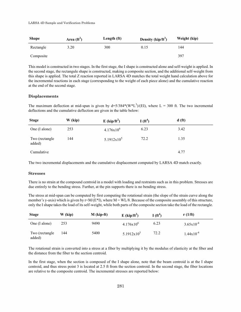
LARSA 4D Sample and Verification Problems
Shape Area (ft2) Length (ft) Density (kip/ft3) Weight (kip)
Rectangle 3.20 300 0.15 144
Composite 397
This model is constructed in two stages. In the first stage, the I shape is constructed alone and self-weight is applied. Inthe second stage, the rectangule shape is constructed, making a composite section, and the additional self-weight fromthis shape is applied. The total Z reaction reported in LARSA 4D matches the total weight hand calculation above forthe incremental reactions in each stage (corresponding to the weight of each piece alone) and the cumulative reactionat the end of the second stage.
Displacements
The maximum deflection at mid-span is given by d=5/384*(W*L3)/(EI), where L = 300 ft. The two incrementaldeflections and the cumulative deflection are given in the table below:
Stage W (kip) E (kip/ft2) I (ft4) d (ft)
One (I alone) 253 4.176x10⁶ 6.23 3.42
Two (rectangleadded)
144 5.1912x10⁵ 72.2 1.35
Cumulative 4.77
The two incremental displacements and the cumulative displacement computed by LARSA 4D match exactly.
Stresses
There is no strain at the compound centroid in a model with loading and restraints such as in this problem. Stresses aredue entirely to the bending stress. Further, at the pin supports there is no bending stress.
The stress at mid-span can be computed by first computing the rotational strain (the slope of the strain curve along themember’s y-axis) which is given by r=M/(E*I), where M = WL/8. Because of the composite assembly of this structure,only the I shape takes the load of its self-weight, while both parts of the composite section take the load of the rectangle.
Stage W (kip) M (kip-ft) E (kip/ft2) I (ft4) r (1/ft)
One (I alone) 253 9490 4.176x10⁶ 6.23 3.65x10⁻⁴
Two (rectangleadded)
144 5400 5.1912x10⁵ 72.2 1.44x10⁻⁴
The rotational strain is converted into a stress at a fiber by multiplying it by the modulus of elasticity at the fiber andthe distance from the fiber to the section centroid.
In the first stage, when the section is composed of the I shape alone, note that the beam centroid is at the I shapecentroid, and thus stress point 3 is located at 2.5 ft from the section centroid. In the second stage, the fiber locationsare relative to the composite centroid. The incremental stresses are reported below:
281

LARSA 4D Sample and Verification Problems
Stage Stress Point Fiber Location (ft) E (kip/ft2) Stress (kip/ft2)
One Point 3 @ Mid-Span -2.5 4.176x10⁶ 3800
Two Point 3 @ Mid-Span -3.044 4.176x10⁶ -1,830
Two Point 5 @ Mid-Span 2.756 5.1912x10⁵ 206
The stresses in LARSA 4D match up to rounding.
Verification of the Time Effect on Elastic ModulusIn a time-dependent analysis, the concrete slab will be affected by the time effect on elastic modulus while the steelpart will remain unchanged. This necessitates a recomputation of the composite member properties. In this examplewe will assume the self-weight loading occurs 15 days after casting.
The effect of time is modeled by multiplying E by f = sqrt(age/(4.0+0.857 X age) ) where age is in days and is nogreater than 28. The concrete E is multiplied by f = 0.943. As above, the location of the composite centroid relativeto the reference line is determined by the following table:
Shape cy (ft) f*E (kip/ft2) A (ft2) f*E*A cy*f*E*A
I -2.9 4.176x10⁶ 1.72 7.182x10⁶ -20.8x10⁶
Rectangle 0 4.895x10⁵ 3.20 1.545x10⁶ 0
Total 8.73x10⁶ -20.8x10⁶
Composite -2.38
Hand calculations for A and Izz follow as described above, except this time we treat the reference material as the time-adjusted concrete.
Shape A (ft2) A*E/E_ref Izz (ft4) Izz+Ac2 (Izz+Ac2)*E/E_ref
I 1.72 14.7 6.23 6.69 57.0
Rectangle 3.20 3.20 0.171 18.3 18.3
Composite 17.9 75.4
LARSA 4D does not report time-adjusted cross-sectional properties.
In LARSA 4D, a Material Time Effect record (with default settings) is applied to the Fc_4 material. The casting dayof the composite member is set to day 0. Self-weight loading is applied on day 15. The CEB-FIP 90 analysis code ischosen, the time effect on elastic modulus is turned on (all other time effects are turned off), and a Time-DependentStaged Construction Analysis is run.
The results in the first stage are unchanged.
282

LARSA 4D Sample and Verification Problems
Displacements
The maximum deflection at mid-span is given by 5/384*(W*L3)/(EI). W and L are as before. E is from the referencematerial, now the time-adjusted concrete property. The revised computation for incremental displacement in the secondstage is:
Stage W (kip) E (kip/ft2) I (ft4) d (ft)
Two (rectangleadded)
144 4.895x10⁵ 75.4 1.37
Stresses
The reviesd stresses are:
Stage W (kip) M (kip-ft) E (kip/ft2) I (ft4) r (1/ft)
Two (rectangleadded)
144 5400 4.895x10⁵ 75.4 1.46x10⁻⁴
The rotational strain is converted into a stress at a fiber by multiplying it by the modulus of elasticity at the fiber andthe distance from the fiber to the section centroid.
In the first stage, when the section is composed of the I shape alone, note that the beam centroid is at the I shapecentroid, and thus stress point 3 is located at 2.5 ft from the section centroid. In the second stage, the fiber locationsare relative to the composite centroid. The incremental stresses are reported below:
Stage Stress Point Fiber Location (ft) E (kip/ft2) Stress (kip/ft2)
Two Point 3 @ Mid-Span -3.044 4.176x10⁶ -1,860
Two Point 5 @ Mid-Span 2.756 4.895x10⁵ 197
The results in LARSA 4D are correct up to rounding.
Verification of ShrinkageTo verify shrinkage, we will look at the total effect of shrinkage between days 15 and 400. Shrinkage, εS as givenbelow according to CEB-FIP 90, is an additional strain added into the cross-section accumulated from time t0 to timet1. In this part, the time effect on elastic modulus is not included.εS(t0, t1) = EcS0 * [BetaS(t1) - BetaS(t0)]
EcS0 = (160 + 10*BetaSC*(9 – Fc_28/10)) /1000000 * (-1.55*(1.0 - (RH/100.)^3))
BetaS(t) = sqrt((t - TS)/(350*((H/100)^2) + (t - TS)))
where TS = 3, BetaSC = 5, H= 2 * Area/Perimeter converted to milimeters, RH is the relative humidity (80%), and t0,t1 are the ages of the section in days. Fc_28 = 27.6 MN/m2 (576 kip/ft2).
Shrinkage in the composite section is due only to the effect of shrinkage in the concrete part. The area of the rectangleis 3.2 ft2 and the perimeter for this example is treated as 9.6 ft (which includes the unexposed perimeter at the interface
283

LARSA 4D Sample and Verification Problems
of the shapes in order to match the perimeter used by LARSA 4D). H = 203.2 mm. Substutiting these values into theformula gives εS(15,400) = -1.33x10⁻⁴.
Because the two shapes that make up the cross-section are connected and governed by the assumption that planesections remain plane, shrinkage will create self-equilibriating stress (also known as eigenstresses) in both the concreteand steel parts of the section.
The computation of self-equilibriating stress due to shrinkage involves combining two equal-and-opposite strains. Thefirst component is the “external” component with magnitude εS in the concrete part (and zero in the steel part), andit is integrated across the fibers that make up the cross-section area to determine an equivalent force F = εS*E*A andmoment M = F*cy imposed at the beam end at the composite centroid. This force and moment determines the actualdeformation of the beam. In Ghali, Favre, and Elbadry (2002) example 5.2, the external component corresponds to theforces and moments that undo the artificial restraint on shrinkage.
Using the E and A values of the concrete part and the distance from the beam centroid to the centroid of the concrete part(the same as the offset of the beam centroid from the beam reference axis given in the first table), F = -222 kip, M = -522kip-ft. The corresponding strain for the composite beam is -2.51x10⁻⁵ pure strain and -1.39x10⁻⁵ 1/ft bending strain.
The second or “internal” component has magnitude -εS at any fiber in the concrete part and zero at any fiber in thesteel part, but it does not cause deformation. It corresponds to Ghali, Favre, and Elbadry’s strain in the section whenshrinkage is restrained.
Self-equilibriating stress at a fiber is the modulus of elasticity at the fiber multiplied by the sum of the strain due to theexternal component (a linear stress profile across the entire cross-section) and the strain due to the internal componentat the fiber (a step function with value -εS in the concrete part and 0 in the steel part).
There are no continuity stresses in a model such as this. Stress is constant along the length of the beam.
The computation of total stress is given in the following table:
Stress Point Fiber Location (ft) E (kip/ft2) Stress (kip/ft2)
Point 3 -3.044 4.176x10⁶ 72.5
Point 5 2.756 5.1912x10⁵ 36.2
The results in LARSA 4D match up to rounding.
284

LARSA 4D Sample and Verification Problems
S08: Time-Dependent MaterialProperties Effects
This sample problem verifies creep and shrinkage strain calculations a wide column modeled using beam and shellelements with dimensions 1.0 × 1.2 m x 0.4 m under vertical loading.
Example Project: The example described here can be found in the Staged Construction folder of your LARSA 4DSamples directory (generally My Documents\LARSA Projects\Samples) in the file S08.
Problem DefinitionA very wide column is subjected to a point load in the gravitational direction. Determine the vertical displacementsdue to creep and shrinkage separately, and compare the values obtained in CEB-FIP 78, CEB-FIP 90, CEB-FIP 2010,EN1992/Eurocode 2004 and AASHTO LRFD v6 codes.
285

LARSA 4D Sample and Verification Problems
Figure 1: Problem Definition
ModelingIn LARSA 4D, the same object is created in two different ways, by using a frame element and a plate element formodeling. The dimensions of both the frame and the plate are 1.0 × 1.2 m and their thickness is 0.4 m. The equivalentloadings are also identical. The point load P is 10,000 kN in magnitude.
286

LARSA 4D Sample and Verification Problems
Figure 2: Problem Definition: the Frame Element (left) and the plate (right).
The frame is supported by a fixed support at the bottom end and the orientation of the member is along the Z-axis. Theplate is supported by a fixed support at the bottom left end (Joint 3) as can be seen in Figure 3. Translation of Joint 4,on the other hand, is left free in the direction of ×. Additionally, to hinder out of plane deformations, top joints (Joints,5 and 6) are restrained the translation in the direction of Y.
Figure 3: Joints of the Frame (left) and the plate (right) from the Front Plane
Material properties of concrete such as Modulus of Elasticity (E), Poisson Ratio, Shear Modulus (G), Fck, ConcreteCement Hardening Type and Material Time-Effect should be entered manually for the both models as shown in Figure4, Figure 5 and Figure 6.
287

LARSA 4D Sample and Verification Problems
Figure 4: Material Properties.
Additional properties for the material under the More Properties segment are given in Figure 5. Material Time Effecthas to be set to take the time dependent material properties for the solution. However, before defining Material TimeEffects , the design code which will be used for the time-effects calculations should be selected from Analysis →Time Dependent Analysis Options → Code For Creep and Shrinkage . In this example, check both Include Creepand Include Shrinkage options. Time effect on elastic modulus is not included.
Figure 5: More Properties
When performing verification for CEB-FIP 78, f rom the Material Time Effects tab, parameters required for theselected code should be defined for the plate and the frame.
288

LARSA 4D Sample and Verification Problems
Figure 6: Material Time Effects for CEB-FIP78
Construction Sequence
Two different construction sequences are considered, Case A and Case B. In both cases, all elements are cast on the 10th
day. Case A models a cast-in-place segment. In Case A, the elements are constructed on the 11th day (i.e. their stiffnessis considered beginning at the age of 1). In Case B a pre-cast model is considered where the elements are constructedon the 25th day (i.e. their stiffness is considered beginning at the age of 15, what happened before than is ignored).
At the age of 16th day of concrete, elements are subjected to external sustained load (construction day 26). In order torepresent that events in the model and get results for the desired ages such as 40th and 100th days, construction stagesshould be defined for those times (50 and 110 days).
Figure 7: Construction Stages
Verification of CreepThe creep and shrinkage displacements can be observed independently. For example, right clicking on the Day 110:Creep in the Analysis Results and selecting the joint displacements will show the cumulative displacements of all theprevious stages, plus the creep displacement of the Day 110 stage, as in Figure 8.
289

LARSA 4D Sample and Verification Problems
Figure 8: Joint Displacements
To get the joint displacements due to creep of the Day 110 stage only, select Extract Creep from the drop down menu.
Figure 9: Joint Displacements due to Creep Deformation in Day 110
Creep formulas provided by each design code are given below. Hand calculations are performed based on theseformulas and the obtained results are compared with the LARSA 4D results.
ParametersRH = 60 (ambient relative humidity, %)
fcm = 40 (mean compressive strength of concrete at the age of 28 days, MPa, Fck + 8 MPa)
t = 100 (age of concrete in days at the moment considered)
t0 = 16 (age of concrete at loading, days)
290

LARSA 4D Sample and Verification Problems
Assumptions
In LARSA 4D, frame elements are considered as column elements, i.e. the perimeter of the cross-section are subjectedto atmosphere. Therefore the V/S ratio and notional thickness become:V/S = (width × thickness × length) / (2(width × length + thickness × length)) = width × thickness / (2 × (width + thickness))
h = 2(V/S) = width × thickness / (width + thickness)
Notional thickness for frame element is calculated as 300 mm.
On the other hand, plate elements are considered as slab elements, accordingly the edges in the direction of thicknessare not subjected to atmosphere.V/S = (width × thickness × length) / (2 × width × length) = thickness / 2
h = 2(V/S) = thickness
Notional thickness for plate element is calculated as 400 mm.
Creep Strain Calculation
Creep strain is calculated by multiplying the strain which is not time-dependent with the creep coefficient.εc(t,t0) = σ / Ec×φ(t,t0)
where,σ is constant stress on the member
Ec is elastic modulus of concrete
φ(t,t0) is creep coefficient
Creep Coefficients
CEB-FIP 78φ(t,t0) = βa(t0)×φd×βd(t - t0) + φf×[βf(t) - βf(t0)]
where,βa is notional thickness coefficient
φd is delayed modulus of elasticity coefficient
βd should be input to LARSA as a time-dependent curve
φf is creep coefficient obtained from φf1×φf2 (φf1 is coefficient of notional thickness and φf2 is environment creep coefficient.)
βf should be input to LARSA as a time-dependent curve
CEB-FIP 90φ(t,t0) = φ0 × βc(t-t0)
where,φ0 = φRH×β(fcm)×β(t0)
φRH = 1 + (1 - (RH/100))/(0.46×(h/100)1/3)
β(fcm) = 5.3 / (fcm/10)0.5
291

LARSA 4D Sample and Verification Problems
β(t0) = 1/(0.1 + t00.2)
βc(t-t0) = [(t - t0)/(βH + t - t0)]0.3
βH = 150×{1 + (1.2×RH/100)18} × (h/100) + 250 ≤ 1500
CEB-FIP 2010φ(t,t0) = φbc(t,t0) + φdc(t,t0)
where,The basic creep coefficient may be estimated from:
φbc(t,t0) = βbc(fcm)×βbc(t,t0)
βbc(fcm) = 1.8/(fcm)0.7
βbc(t,t0) = ln((30/t0,adj) + 0.035)2 ×(t-t0) + 1)
The drying creep coefficient may be estimated from:
φdc(t,t0) = βdc(fcm)×β(RH)×βdc(t0)×βdc(t,t0)
βdc(fcm) = 412/(fcm)1.4
β(RH) = (1-RH/100)/(0.1×h/100)1/3
βdc(t0) = 1/(0.1 + (t0,adj)0.2)
EN1992/EuroCode 2004ϕ(t,t0) = ϕ0×βc(t,t0)
where,φ0 = φRH×β(fcm)×β(t0)
φRH = 1 + ((1 - RH/100)/(0.1×h1/3)) for fcm ≤ 35 MPa
φRH = 1 + ((1 - RH/100)/(0.1×h1/3)×α1)×α2 for fcm > 35 MPa
β(fcm) = 16.8 / (fcm)0.5
β(t0) = 1 / (0.1 + t00.2)
βc(t,t0) = [(t - t0) / (βH + t - t0)]0.3
βH = 1.5×[1 + (0.012×RH)18]×h + 250 ≤ 1500 for fcm ≤ 35 MPa
βH = 1.5×[1 + (0.012×RH)18]×h + 250×α3 ≤ 1500×α3 for fcm > 35 MPa
α1 = [35 / fcm]0.7
α2 = [35 / fcm]0.2
α3 = [35 / fcm]0.5
AASHTO LRFD v6
φ(t,t0) = 1.9×ks×khc×kf×ktd×t0-0.118
292

LARSA 4D Sample and Verification Problems
where,ks = 1.45 – 0.13(V/S) ≥ 1.0 (V/S in inch)
khc = 1.56 – 0.008×RH
kf = 5/(1 + f'ci)
ktd = (t - t0)/(61 - 4×f'ci + t - t0)
fʹci = 0.80×fʹc (ksi).
fʹc is characteristic compressive strength of concrete at age of 28 days.
Both cases (Case A and Case B) gives the same results for the creep calculation since they are loaded at the same agewhich is later than the construction of both groups.
Creep Displacements of Frame Elements (Units are in mm)
Code Hand Calc. LARSA 4D Error (%)
CEB-FIP 78 -0.759 -0.759 0.0
CEB-FIP 90 -0.702 -0.703 0.0
CEB-FIP 2010 -0.691 -0.691 0.0
EN1992/Eurocode 2004 -0.664 -0.668 0.0
AASHTO LRFD v6 -0.603 -0.603 0.0
Creep Displacements of Plate Elements (Units are in mm)
Code Hand Calc. LARSA 4D Error (%)
CEB-FIP 78 -0.711 -0.711 0.0
CEB-FIP 90 -0.644 -0.644 0.0
CEB-FIP 2010 -0.659 -0.659 0.0
EN1992/Eurocode 2004 -0.610 -0.614 -1.0
AASHTO LRFD v6 -0.603 -0.603 0.0
LARSA 4D's creep computations match exactly with hand calculations.
Verification of ShrinkageFor the shrinkage displacements of Day 110 stage only, follow the same procedure as before, this time by right clickingDay 110: Shrinkage and extracting the results for shrinkage.
Unlike in the case of creep, Case A and Case B do not undergo the same shrinkage. So the results are presented indifferent tables for each case.
293

LARSA 4D Sample and Verification Problems
Figure 11: Joint Displacements due to Shrinkage Deformation in 110 days
Shrinkage formulas provided by each design code are given below. Hand calculations are performed based on theseformulas and the obtained results are compared with the LARSA 4D results.
ParametersRH = 60 (ambient relative humidity, %)
fcm = 40 (mean compressive strength of concrete at the age of 28 days, MPa, Fck + 8 MPa)
t = 100 (age of concrete in days at the moment considered)
Assumptions
Age of concrete at the beginning of shrinkage or swelling, ts (days) is
ts = 3 days for CEB-FIP 90 and CEB-FIP 2010
ts = 14 days for EN1992/Eurocode 2004
ts = 0 day for AASHTO LRFD v6
Any ts value greater than 0 can be used by defining the input parameters required for CEB-FIP 78 code.
The assumption for notional thickness calculation discussed in creep section is also valid for the shrinkage calculations.
In LARSA 4D, shrinkage occurs only in the time interval between the construction day and time of the momentconsidered. Shrinkage induced displacement before the construction day, accordingly, is ignored.
Shrinkage Strain Calculation
CEB-FIP 78εsh(t,ts) = εs0[βs(t) - βs(ts)]
where,
294

LARSA 4D Sample and Verification Problems
εs0 is shrinkage coefficient obtained from εs1 × εs2 (εs1 is environment shrinkage coefficient and εs2 is the notational thicknessshrinkage coefficient)
βs should be input to LARSA as a curve
CEB-FIP 90εsh(t,ts) = εcso×βs(t-ts)
where,εcso = εs(fcm)×βRH
εs(fcm) = [160 + 10×βsc×(9 - fcm/10]×10-6
βsc is a coefficient which depends on the type of cement (4 for slowly hardening cements SL, 5 for normal or rapid hardeningcements N and R, and 8 for rapid hardening high strength cements RS)
βRH = -1.55×βsRH for 40% ≤ RH ≤ 99%
βRH = 0.25 for RH ≥ 99%
βsRH = 1 - (RH / 100)3
βs(t-ts) = [(t - ts) / (350×(h/100)2 + t - ts)]0.5
CEB-FIP 2010εsh(t,ts) = εcbs(t) + εcds(t,ts)
where,εcbs(t) = εcbs0(fcm)×βbs(t)
εcds(t,ts) = εcds0(fcm)×βRH(RH)×βds(t-ts)
εcbs0(fcm) = -αbs((fcm/10)/(6 + fcm/10))2.5×10-6
βbs(t) = 1-exp(-0.2×t0.5)
εcds0(fcm) = [(220 + 110×αds1)×exp(-αds2×fcm)]×10-6
βRH = -1.55×[1-(RH/100)3] for 40 ≤ RH ≤ 99% × βs1
βRH = 0.25 for RH ≥ 99% × βs1
βds(t-ts) = [(t-ts)/(0.035×h2 + (t-ts))]0.5
βs1 = (35/fcm)0.1 ≤ 1.0
αds1 and αds2: Coefficients dependent on the type of cement
EN1992/EuroCode 2004εsh = εcd + εca
where,The development of the drying shrinkage strain in time follows from:
εcd(t) = βds(t,ts)×kh×εcd,0
kh is a coefficient depending on the notional size h
295

LARSA 4D Sample and Verification Problems
βds(t,ts) = (t-ts)/((t-ts)+0.04×h3/2)
εcd,0 is taken from Table 3.2 in code.
The autogenous shrinkage strain follows from:
εca(t) = βas(t)×εca(∞)
εca(∞) = 2.5×(fck – 10)×10-6
βas(t) = 1 – exp(– 0.2t0.5)
AASHTO LRFD v6
εsh = ks×khc×kf×ktd×0.48×10⁻³
where,khs = (2.00 – 0.014×H)
ktd = (t - ts/(61 - 4×f'ci + t - ts)
The other constants are obtained the same way as in the creep specification.
Shrinkage Displacements of Frame Elements in Group A (Units are in mm)
Code Hand Calc. LARSA 4D Error (%)
CEB-FIP 78 -0.053 -0.053 0.0
CEB-FIP 90 -0.086 -0.086 0.0
CEB-FIP 2010 -0.134 -0.134 0.0
EN1992/Eurocode 2004 -0.130 -0.130 0.0
AASHTO LRFD v6 -0.392 -0.392 0.0
Shrinkage Displacements of Plate Elements in Group A (Units are in mm)
Code Hand Calc. LARSA 4D Error (%)
CEB-FIP 78 -0.035 -0.035 0.0
CEB-FIP 90 -0.065 -0.065 0.0
CEB-FIP 2010 -0.113 -0.113 0.0
EN1992/Eurocode 2004 -0.102 -0.102 0.0
AASHTO LRFD v6 -0.392 -0.392 0.0
Shrinkage Displacements of Frame Elements in Group B (Units are in mm)
Code Hand Calc. LARSA 4D Error (%)
CEB-FIP 78 -0.043 -0.043 0.0
296

LARSA 4D Sample and Verification Problems
Code Hand Calc. LARSA 4D Error (%)
CEB-FIP 90 -0.055 -0.055 0.0
CEB-FIP 2010 -0.078 -0.078 0.0
EN1992/Eurocode 2004 -0.109 -0.109 0.0
AASHTO LRFD v6 -0.259 -0.259 0.0
LARSA's shrinkage computations match exactly with the hand calculations.
297

LARSA 4D Sample and Verification Problems
298

LARSA 4D Sample and Verification Problems
S08b: Time-Dependent MaterialProperties Effects
This sample problem verifies creep and shrinkage strain calculations a wide column modeled using a shell elementwith dimensions 0.4 x 1.0 m x 0.1 m with loading in the gravitational and lateral directions.
Example Project: The example described here can be found in the Staged Construction folder of your LARSA 4DSamples directory (generally My Documents\LARSA Projects\Samples) in the file S08.
Problem DefinitionA column modeled with a shell element is subjected to two point loads of 10,000 kN magnitude in the gravitationaland lateral directions, as shown in Figure 1. Determine the vertical displacements and also the horizontal displcementsin the direction of x due to creep and shrinkage separately, and compare the values obtained in CEB-FIP 78, CEB-FIP90, CEB-FIP 2010, EN1992/Eurocode 2004 and AASHTO LRFD v6 codes.
299
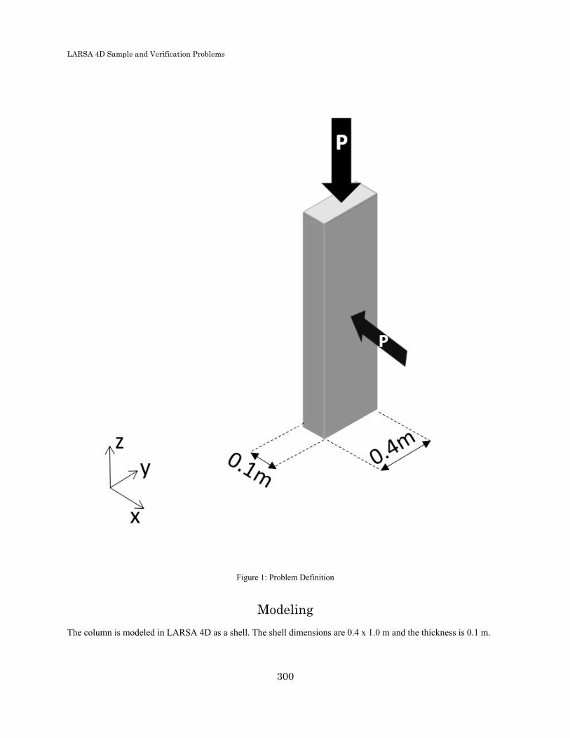
LARSA 4D Sample and Verification Problems
Figure 1: Problem Definition
ModelingThe column is modeled in LARSA 4D as a shell. The shell dimensions are 0.4 x 1.0 m and the thickness is 0.1 m.
300

LARSA 4D Sample and Verification Problems
Figure 2: the Model
Joints of the shell can be seen in figure 2 below. Joint 7 is a fixed support. Joint 8 is free in Translation-X, joint 10is free in Translation-Z and joint 9 is free in the Translation-X and Translation-Z directions. The orientation of themember is along the Z-axis.
301

LARSA 4D Sample and Verification Problems
Figure 3: Joints from the Front Plane
The material properties of concrete were entered manually as shown in Figure 4.
302
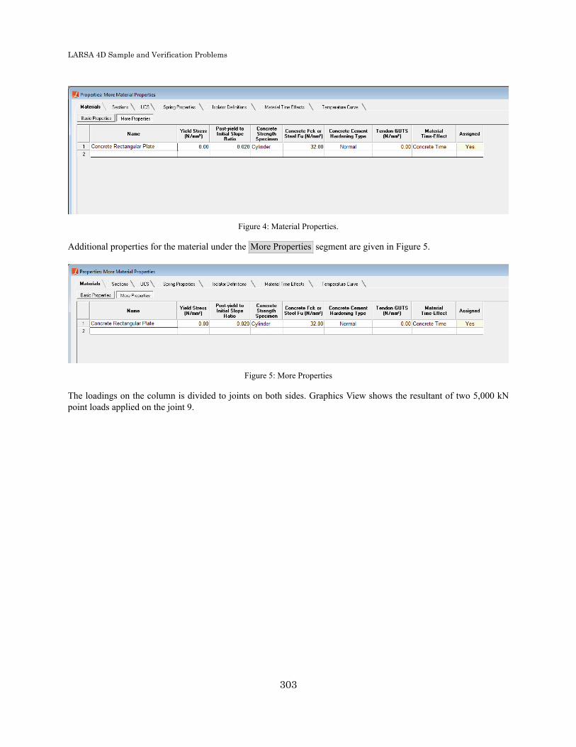
LARSA 4D Sample and Verification Problems
Figure 4: Material Properties.
Additional properties for the material under the More Properties segment are given in Figure 5.
Figure 5: More Properties
The loadings on the column is divided to joints on both sides. Graphics View shows the resultant of two 5,000 kNpoint loads applied on the joint 9.
303

LARSA 4D Sample and Verification Problems
Figure 6: Loading
304
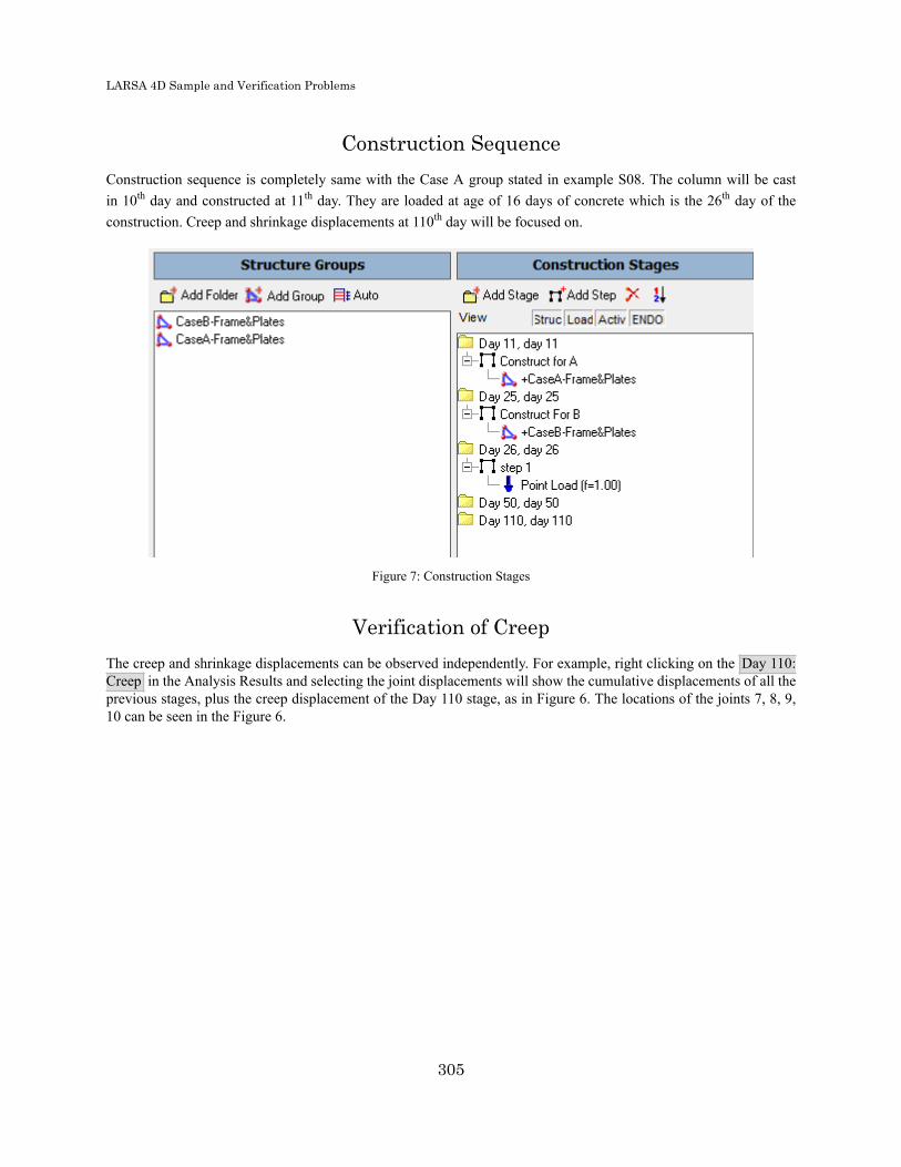
LARSA 4D Sample and Verification Problems
Construction SequenceConstruction sequence is completely same with the Case A group stated in example S08. The column will be castin 10th day and constructed at 11th day. They are loaded at age of 16 days of concrete which is the 26th day of theconstruction. Creep and shrinkage displacements at 110th day will be focused on.
Figure 7: Construction Stages
Verification of CreepThe creep and shrinkage displacements can be observed independently. For example, right clicking on the Day 110:Creep in the Analysis Results and selecting the joint displacements will show the cumulative displacements of all theprevious stages, plus the creep displacement of the Day 110 stage, as in Figure 6. The locations of the joints 7, 8, 9,10 can be seen in the Figure 6.
305

LARSA 4D Sample and Verification Problems
Figure 6: Joint Displacements
To get the joint displacements due to creep of the Day 110 stage only, select Extract Creep from the drop down menu.
Figure 7: Joint Displacements due to Creep Deformation in 110 days
Hand calculations are performed based on these formulas and the obtained results are compared with the LARSA 4Dresults.
ParametersRH = 60 (ambient relative humidity, %)
fcm = 40 (mean compressive strength of concrete at the age of 28 days, MPa, Fck + 8 MPa)
t = 100 (age of concrete in days at the moment considered)
t0 = 16 (age of concrete at loading, days)
Construction Day = 1 (after casting)
306

LARSA 4D Sample and Verification Problems
Assumptions
In LARSA 4D, plate elements are considered as slab elements accordingly the edges in the direction of thickness arenot subjected to atmosphere.V/S = (width × thickness × length) / (2 × width × length) = thickness / 2
h = 2(V/S) = thickness
Notional thickness for plate element is calculated as 400 mm.
Creep Displacements (Units are in mm)
Code Hand Calc. X DisplacementX
Error (%) Hand Calc. Z DisplacementZ
Error (%)
CEB-FIP 78 -0.085 -0.085 0.0 -8.527 -8.536 0.0
CEB-FIP 90 -0.077 -0.077 0.0 -7.722 -7.723 0.0
CEB-FIP2010
-0.079 -0.079 0.0 -7.904 -7.904 0.0
EN1992/Eurocode2004
-0.073 -0.074 -1.0 -7.314 -7.369 -1.0
AASHTOLRFD v6
-0.072 -0.072 0.0 -7.236 -7.235 0.0
LARSA 4D's creep computations match exactly.
Verification of ShrinkageFor the shrinkage displacements of Day 110 stage only, follow the same procedure as before, this time by right clickingDay 110: Shrinkage and extracting the results for shrinkage.
LARSA 4D reports only the shrinkage deformations after the construction day and in the exmple construction day (1)is less than the ts except for AASHTO LRFD v6.
307
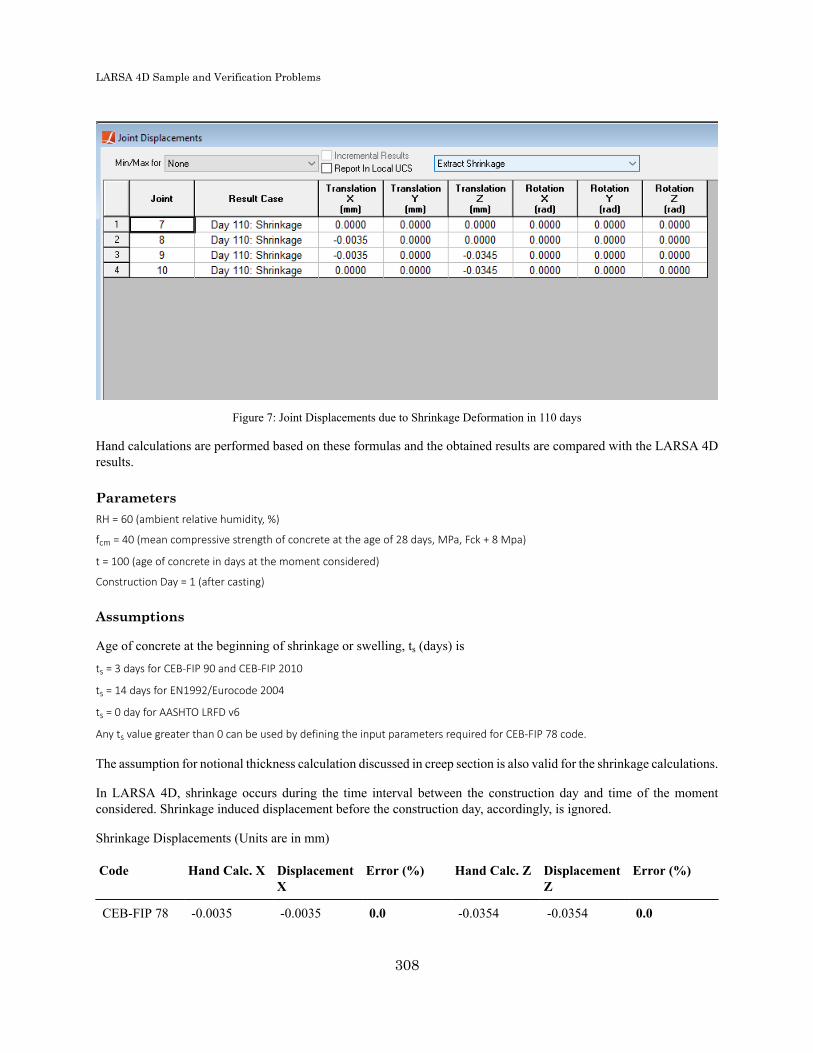
LARSA 4D Sample and Verification Problems
Figure 7: Joint Displacements due to Shrinkage Deformation in 110 days
Hand calculations are performed based on these formulas and the obtained results are compared with the LARSA 4Dresults.
ParametersRH = 60 (ambient relative humidity, %)
fcm = 40 (mean compressive strength of concrete at the age of 28 days, MPa, Fck + 8 Mpa)
t = 100 (age of concrete in days at the moment considered)
Construction Day = 1 (after casting)
Assumptions
Age of concrete at the beginning of shrinkage or swelling, ts (days) is
ts = 3 days for CEB-FIP 90 and CEB-FIP 2010
ts = 14 days for EN1992/Eurocode 2004
ts = 0 day for AASHTO LRFD v6
Any ts value greater than 0 can be used by defining the input parameters required for CEB-FIP 78 code.
The assumption for notional thickness calculation discussed in creep section is also valid for the shrinkage calculations.
In LARSA 4D, shrinkage occurs during the time interval between the construction day and time of the momentconsidered. Shrinkage induced displacement before the construction day, accordingly, is ignored.
Shrinkage Displacements (Units are in mm)
Code Hand Calc. X DisplacementX
Error (%) Hand Calc. Z DisplacementZ
Error (%)
CEB-FIP 78 -0.0035 -0.0035 0.0 -0.0354 -0.0354 0.0
308

LARSA 4D Sample and Verification Problems
Code Hand Calc. X DisplacementX
Error (%) Hand Calc. Z DisplacementZ
Error (%)
CEB-FIP 90 -0.0065 -0.0065 0.0 -0.0650 -0.0650 0.0
CEB-FIP2010
-0.0113 -0.0113 0.0 -0.1130 -0.1130 0.0
EN1992/Eurocode2004
-0.0102 -0.0102 0.0 -0.1020 -0.1020 0.0
AASHTOLRFD v6
-0.0392 -0.0392 0.0 -0.3920 -0.3920 0.0
LARSA 4D's shrinkage computations match exactly with the hand calculations for both directions.
309

LARSA 4D Sample and Verification Problems
310

LARSA 4D Sample and Verification Problems
S09: Plates with Time-DependentMaterial Effects
This sample problem verifies time dependent elastic modulus change, creep and shrinkage strain calculations a widecolumn discussed in S08 sample modeled using quadrilateral and triangular shell elements under vertical loading.
Example Project: The example described here can be found in the Staged Construction folder ofyour LARSA 4D Samples directory (generally My Documents\LARSA Projects\Samples) in the fileS09_CEBFIP90_CreepShrinkage_AxialForce.
Problem DefinitionA very wide column is subjected to a point load in the gravitational direction. Determine the vertical displacementsdue to creep and shrinkage separately, and compare the values obtained in CEB-FIP 90 code.
311
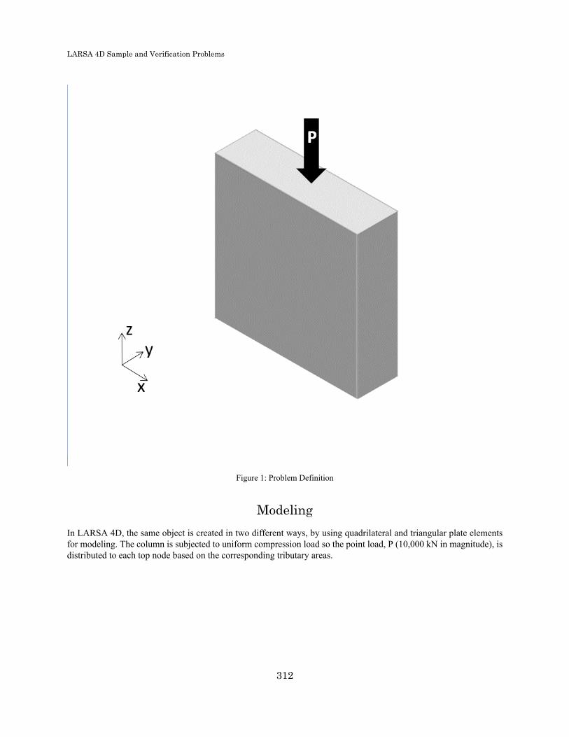
LARSA 4D Sample and Verification Problems
Figure 1: Problem Definition
ModelingIn LARSA 4D, the same object is created in two different ways, by using quadrilateral and triangular plate elementsfor modeling. The column is subjected to uniform compression load so the point load, P (10,000 kN in magnitude), isdistributed to each top node based on the corresponding tributary areas.
312

LARSA 4D Sample and Verification Problems
Figure 2: Problem Definition: the Quad Mesh (left) and the Triangle Mesh (right).
The models are supported by a fixed support at the bottom left end (Joint 3) as can be seen in Figure 2. Translation ofJoints 4, 13, 17, and 21, on the other hand, is left free in the direction of ×. Additionally, to provide stiffness for theout of plane direction, bottom nodes are restrained the rotation about direction of ×.
Material properties of concrete such as Modulus of Elasticity (E), Poisson Ratio, Shear Modulus (G), Fck, ConcreteCement Hardening Type and Material Time-Effect are same with the CEB-FIP90 case of the previous example. Inaddition, time dependent elastic modulus curve is defined (Figure 3).
Figure 3: Time vs Elastic Modulus.
The same construction sequence with the previous example is acted and one more stage (Day 111) is added in whichthe axial force is acted one more time.
313

LARSA 4D Sample and Verification Problems
Figure 4: Construction Sequence
Verification of CreepThe creep and shrinkage displacements can be observed independently. For example, right clicking on the Day 110:Creep in the Analysis Results and selecting the joint displacements will show the cumulative displacements of all theprevious stages, plus the creep displacement of the Day 110 stage.
Creep Displacements (Units are in mm)
OutputParameter
Hand Calc. LARSA 4DQuad-Bilinear
LARSA 4DQuad-Incomp.
LARSA 4DQuad-Drilling
LARSA 4DQuad-MITC4
LARSA 4DTriangle-Bilinear
Average of Jt.5,6,14,18,22
-0.644 -0.644 (0%) -0.644 (0%) -0.644 (0%) -0.644 (0%) -0.644 (0%)
LARSA 4D's creep computations match exactly with hand calculations.
Verification of ShrinkageFor the shrinkage displacements of Day 110 stage only, follow the same procedure as before, this time by right clickingDay 110: Shrinkage and extracting the results for shrinkage.
Shrinkage Displacements (Units are in mm)
OutputParameter
Hand Calc. LARSA 4DQuad-Bilinear
LARSA 4DQuad-Incomp.
LARSA 4DQuad-Drilling
LARSA 4DQuad-MITC4
LARSA 4DTriangle-Bilinear
Average of Jt.5,6,14,18,22
-0.065 -0.065 (0%) -0.065 (0%) -0.065 (0%) -0.065 (0%) -0.065 (0%)
314

LARSA 4D Sample and Verification Problems
LARSA's shrinkage computations match exactly with the hand calculations.
Verification of Elastic Modulus ChangeFor the elastic modulus change verification, incremental displacement ratio at Day 26 and Day 111 stages (Uz26 /Uz111) are inversely proportional with the ratio of elastic modulus at corresponding stages ((E111 / E26), this time byright clicking Day 111: Step 1 and checking the Incremental Results.
Vertical Displacement Ratios (Uz@ Day 26 / Uz@ Day 111) (Units are in mm)
OutputParameter
ElasticModulusRatio(E111 / E26)
LARSA 4DQuad-Bilinear
LARSA 4DQuad-Incomp.
LARSA 4DQuad-Drilling
LARSA 4DQuad-MITC4
LARSA 4DTriangle-Bilinear
Average of Jt.5,6,14,18,22
1.29 1.29 (0%) 1.29 (0%) 1.29 (0%) 1.29 (0%) 1.29 (0%)
315

LARSA 4D Sample and Verification Problems
316

LARSA 4D Sample and Verification Problems
S09b: Plates with Time-DependentMaterial Effects (Orthotropic
Material)
This sample problem verifies time dependent elastic modulus change, creep and shrinkage strain calculations a widecolumn discussed in S08 sample modeled using quadrilateral and triangular shell elements with orthotropic materialsunder vertical loading.
Example Project: The example described here can be found in the Staged Construction folder ofyour LARSA 4D Samples directory (generally My Documents\LARSA Projects\Samples) in the fileS09b_CEBFIP90_CreepShrinkageVarE_AxialForce.
Problem DefinitionA very wide column is subjected to a point load in the gravitational direction. Determine the vertical displacementsdue tovarying elastic modulus, creep and shrinkage separately, and compare the values obtained in CEB-FIP 90 code.
317

LARSA 4D Sample and Verification Problems
Figure 1: Problem Definition
ModelingThe models used for S09 are regenerated by assigning orthotropic material with the same isotropic material properties.The column is subjected to uniform compression load so the point load, P (10,000 kN in magnitude), is distributed toeach top node based on the corresponding tributary areas.
318
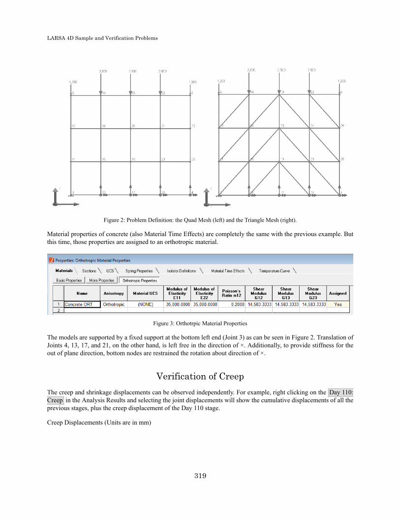
LARSA 4D Sample and Verification Problems
Figure 2: Problem Definition: the Quad Mesh (left) and the Triangle Mesh (right).
Material properties of concrete (also Material Time Effects) are completely the same with the previous example. Butthis time, those properties are assigned to an orthotropic material.
Figure 3: Orthotrpic Material Properties
The models are supported by a fixed support at the bottom left end (Joint 3) as can be seen in Figure 2. Translation ofJoints 4, 13, 17, and 21, on the other hand, is left free in the direction of ×. Additionally, to provide stiffness for theout of plane direction, bottom nodes are restrained the rotation about direction of ×.
Verification of CreepThe creep and shrinkage displacements can be observed independently. For example, right clicking on the Day 110:Creep in the Analysis Results and selecting the joint displacements will show the cumulative displacements of all theprevious stages, plus the creep displacement of the Day 110 stage.
Creep Displacements (Units are in mm)
319

LARSA 4D Sample and Verification Problems
OutputParameter
Hand Calc. LARSA 4DQuad-Bilinear
LARSA 4DQuad-Incomp.
LARSA 4DQuad-Drilling
LARSA 4DTriangle-Bilinear
Average of Jt.5,6,14,18,22
-0.644 -0.644 (0%) -0.644 (0%) -0.644 (0%) -0.644 (0%)
LARSA 4D's creep computations match exactly with hand calculations.
Verification of ShrinkageFor the shrinkage displacements of Day 110 stage only, follow the same procedure as before, this time by right clickingDay 110: Shrinkage and extracting the results for shrinkage.
Shrinkage Displacements (Units are in mm)
OutputParameter
Hand Calc. LARSA 4DQuad-Bilinear
LARSA 4DQuad-Incomp.
LARSA 4DQuad-Drilling
LARSA 4DTriangle-Bilinear
Average of Jt.5,6,14,18,22
-0.065 -0.065 (0%) -0.065 (0%) -0.065 (0%) -0.065 (0%)
LARSA's shrinkage computations match exactly with the hand calculations.
Verification of Elastic Modulus ChangeFor the elastic modulus change verification, incremental displacement ratio at Day 26 and Day 111 stages (Uz26 /Uz111) are inversely proportional with the ratio of elastic modulus at corresponding stages ((E111 / E26), this time byright clicking Day 111: Step 1 and checking the Incremental Results.
Vertical Displacement Ratios (Uz@ Day 26 / Uz@ Day 111) (Units are in mm)
OutputParameter
Elastic ModulusRatio(E111 / E26)
LARSA 4DQuad-Bilinear
LARSA 4DQuad-Incomp.
LARSA 4DQuad-Drilling
LARSA 4DTriangle-Bilinear
Average of Jt.5,6,14,18,22
1.29 1.29 (0%) 1.29 (0%) 1.29 (0%) 1.29 (0%)
320

LARSA 4D Sample and Verification Problems
Samples for Influence-BasedAnalysis
These samples provide an overview of the influence line and surface analysis.
For More Information, please refer to the following documentation.
• For help on influence line and surface analysis, see Influence Line & Surface Analysis in LARSA 4D ReferenceManual.
INF01: AASHTO LFD Simple Span 323Model Setup 323Result Case Setup 324Accessing Results 325Solution Comparison 327
INF02: AASHTO LFD Three Span 329Model Setup 329Span Break Markers 331Result Case Setup 332Accessing Results 334
INF10: Influence Surface 337Model Setup 337Result Case Setup 337Accessing Results 337
321

LARSA 4D Sample and Verification Problems
322

LARSA 4D Sample and Verification Problems
INF01: AASHTO LFD Simple Span
A single simply-supported span is loaded according to AASHTO LFD's live load specifications using influence lines.
Example Project: The example described here can be found in the Influence folder of your LARSA 4D Samplesdirectory (generally My Documents\LARSA Projects\Samples) in the file INF01.
Model SetupThis model consists of a single 200-foot span divided into 10 members of equal length. The left end at (0,0,0) is fullysupported in translation and left free in rotation. The right end at (200,0,0) is supported in z-translation only. UniversalRestraints [in LARSA 4D User’s Manual] are used to support all joints in y-translation and x- and z-rotation, reducingthe model to two dimensions in the X-Z plane.
Sample INF01
A lane [see “Lanes” in LARSA 4D Reference Manual], named "LL Lane," is created along the length of the span. Aunit load will march along the lane to generate the influence line coefficients. To create the lane, you can use the Draw> From Selected Members > Lane command.
323

LARSA 4D Sample and Verification Problems
The standard moving load database is connected to the project [see “Connecting Databases” in LARSA 4D User’sManual].
To create the influence line coefficients, a moving load case must be set up. In the Load Cases Explorer [in LARSA4D User’s Manual] a load case named "Influence Load" is created. In the case, a single moving load is applied withthe following specification:
Lane Loaded Load Pattern Applied LoadDirection
Load Factor Direction of Travel
LL Lane INFLUENCELOAD Global -Z 1.00 Forward
The Linear Moving Load/Influence analysis is run on the model.
Result Case SetupAfter the analysis, influence-based cases are created for the different types of AASHTO LFD loading. Using Results> Influence Line/Surface Case command three times, separate cases are created:
LL Lane/HL-93 Design TruckThis case specifies the loading of a HL-93 Design Truck, which is the HS20-44 truck with the rear axlevariably positioned between 14 and 30 feet behind the previous axle. The vehicle is defined in the standardmoving load database and so is available because the database was connected earlier.
LL Lane/HL-93 Design Truck
324
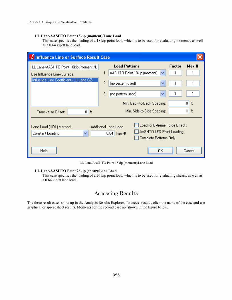
LARSA 4D Sample and Verification Problems
LL Lane/AASHTO Point 18kip (moment)/Lane LoadThis case specifies the loading of a 18 kip point load, which is to be used for evaluating moments, as wellas a 0.64 kip/ft lane load.
LL Lane/AASHTO Point 18kip (moment)/Lane Load
LL Lane/AASHTO Point 26kip (shear)/Lane LoadThis case specifies the loading of a 26 kip point load, which is to be used for evaluating shears, as well asa 0.64 kip/ft lane load.
Accessing ResultsThe three result cases show up in the Analysis Results Explorer. To access results, click the name of the case and usegraphical or spreadsheet results. Moments for the second case are shown in the figure below.
325

LARSA 4D Sample and Verification Problems
Moments from Concentrated + Lane Load
LARSA will not automatically switch between the 18 and 26 kip loads depending on whether you are investigatingshears or moments. The engineer is responsible for using the appropriate result case for each investigation.
You may check where LARSA decided to place the truck and point loads to produce the maximum effect for any pointon the structure using the graphical influence coefficient view [see “Influence Coefficients Graphical View” in LARSA4D User’s Manual]. An image of that is shown below. Arrows indicate the locations of the axles of the HL-93 DesignTruck to produce the maximum moment at the first station of the sixth member.
326
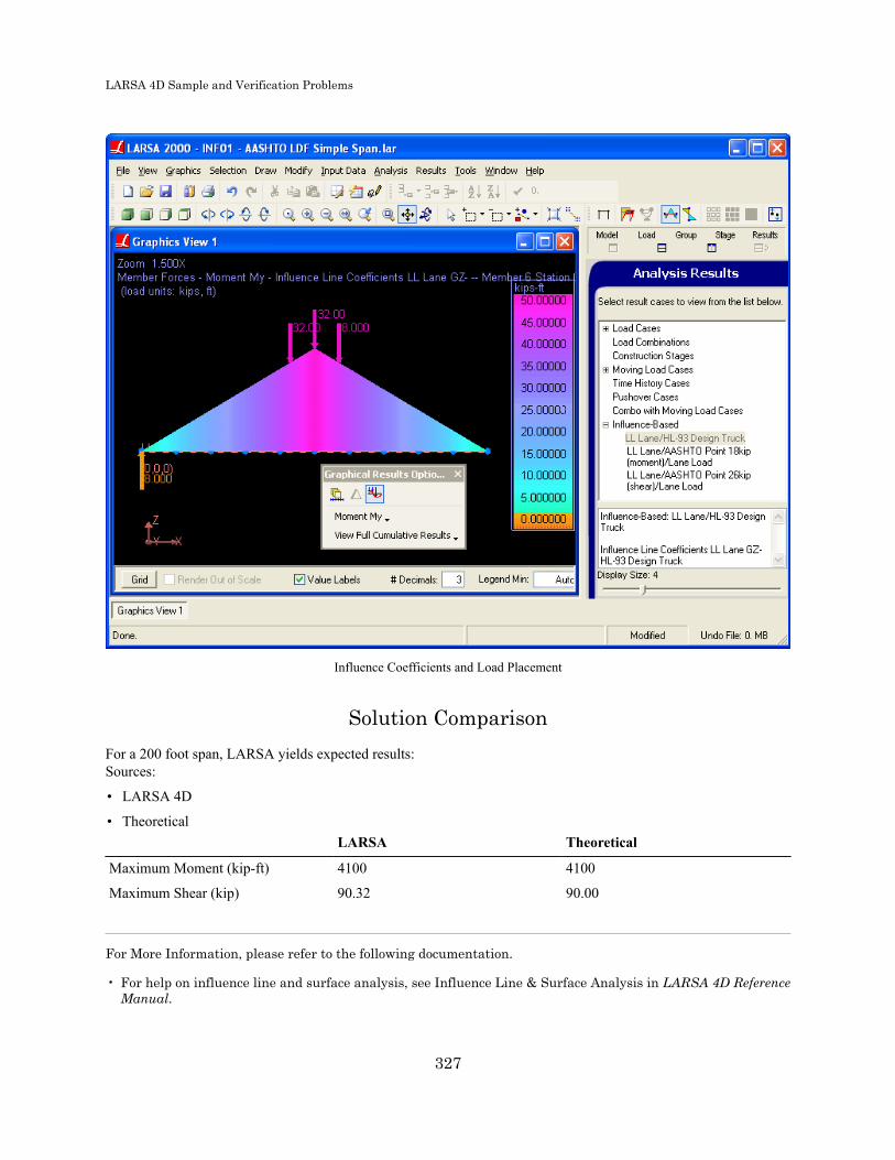
LARSA 4D Sample and Verification Problems
Influence Coefficients and Load Placement
Solution ComparisonFor a 200 foot span, LARSA yields expected results:Sources:
• LARSA 4D
• TheoreticalLARSA Theoretical
Maximum Moment (kip-ft) 4100 4100
Maximum Shear (kip) 90.32 90.00
For More Information, please refer to the following documentation.
• For help on influence line and surface analysis, see Influence Line & Surface Analysis in LARSA 4D ReferenceManual.
327

LARSA 4D Sample and Verification Problems
328

LARSA 4D Sample and Verification Problems
INF02: AASHTO LFD Three Span
A three-span curved bridge is loaded according to AASHTO LFD's live load specifications using influence lines. Thisexample illustrates the use of bridge paths and span break makers.
Example Project: The example described here can be found in the Influence folder of your LARSA 4D Samplesdirectory (generally My Documents\LARSA Projects\Samples) in the file INF02.
Sample INF02
Model SetupThis model consists of a 200-foot bridge in three spans of length 60, 80, and 60 feet. The bridge is divided into membersof 20 feet each (span 1: members 1-3; span 2: members 4-7; span 3: members 8-10). The end joints are fully supported.The intermediate supports are simply supported, supported in translation but not rotation.
The bridge is curved using Bridge Paths [in LARSA 4D Reference Manual]. A bridge path coordinate system is definedas follows:
329

LARSA 4D Sample and Verification Problems
Bridge Path
With the bridge coordinate system set as the active coordinate system, the coordinates of the joints are simply spaced20-feet along the station axis.
330

LARSA 4D Sample and Verification Problems
Joint coordinates with the bridge path coordinate system active
The lane and moving load case setup are identical as in the previous sample: INF01: AASHTO LFD Simple Span(page 323).
Span Break MarkersAASHTO LFD Section 3.11.3 provides that for the determination of maximum negative moments, two concentratedloads on different spans must be considered. It is possible to specify that two point loads be applied using influencelines, but a special feature has been added that ensures 1) that a second load is only considered for negative moments,and 2) that the second concentrated load is applied on a different span than the first concentrated load.
LARSA cannot automatically determine where one span ends and another span begins. In complex bridge models, thelocations of supports at spans are not located near the deck where the influence lines are considered but at the base ofpiers. So LARSA needs to be informed where one span ends and another begins on the lane path definition.
The lane path definition is amended by inserting Span Break markers after the last geometry point of each span. Inthis example, the first span ends after the third member, member 3. However, the last geomety point on the span isthe geometry point at the start of member 4. A span break marker goes after this row to indicate that the first spancontains member 3. If a marker were placed after the geometry point at the start of member 3, the first span would goonly as far as the beginning of member 3, not to its end.
The second span break marker is placed four rows later, after the row for the geometry point at the start of member8. This makes the middle span contain members 4, 5, 6, and 7.
331

LARSA 4D Sample and Verification Problems
Span break markers added to the lane path definition
Result Case SetupThe result case setup for the vehicle load pattern and the 26 kip concentrated load for shear using influence-basedresults is identical to the previous sample: INF01: AASHTO LFD Simple Span (page 323).
The setup for the 18 kip concentrated load for negative moment is slightly different. The load is set with Max # to 2,since there can be at most two loads applied. In addition, the AASHTO LFD Point Loading option is checked.
332
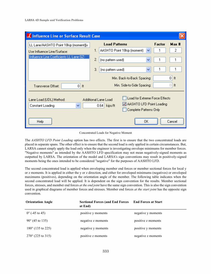
LARSA 4D Sample and Verification Problems
Concentrated Loads for Negative Moment
The AASHTO LFD Point Loading option has two effects. The first is to ensure that the two concentrated loads areplaced in separate spans. The other effect is to ensure that the second load is only applied in certain circumstances. But,LARSA cannot simply apply the load only when the engineer is investigating envelope minimums for member forces."Negative moments" as intended by the AASHTO LFD specification may not mean negatively-signed moments asoutputted by LARSA. The orientation of the model and LARSA's sign conventions may result in positively-signedmoments being the ones intended to be considered "negative" for the purposes of AASHTO LFD.
The second concentrated load is applied when enveloping member end forces or member sectional forces for local yor z moments. It is applied in either the y or z direction, and either for enveloped minimums (negatives) or envelopedmaximums (positives), depending on the orientation angle of the member. The following table indicates when thesecond concentrated load will be applied. It is dependent on the sign convention for the results. Member sectionalforces, stresses, and member end forces at the end joint have the same sign convention. This is also the sign conventionused in graphical diagrams of member forces and stresses. Member end forces at the start joint has the opposite signconvention.
Orientation Angle Sectional Forces (and End Forcesat End)
End Forces at Start
0° (-45 to 45) positive y moments negative y moments
90° (45 to 135) negative z moments positive z moments
180° (135 to 225) negative y moments positive y moments
270° (225 to 315) positive z moments negative z moments
333
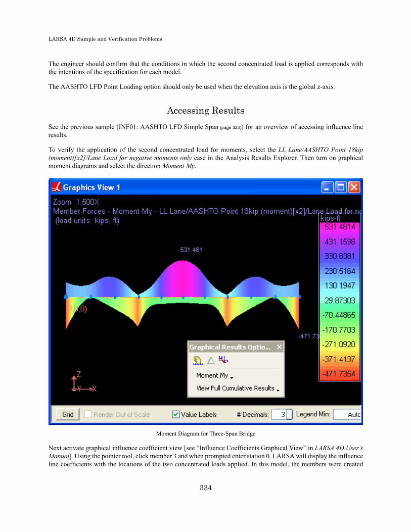
LARSA 4D Sample and Verification Problems
The engineer should confirm that the conditions in which the second concentrated load is applied corresponds withthe intentions of the specification for each model.
The AASHTO LFD Point Loading option should only be used when the elevation axis is the global z-axis.
Accessing ResultsSee the previous sample (INF01: AASHTO LFD Simple Span (page 323)) for an overview of accessing influence lineresults.
To verify the application of the second concentrated load for moments, select the LL Lane/AASHTO Point 18kip(moment)[x2]/Lane Load for negative moments only case in the Analysis Results Explorer. Then turn on graphicalmoment diagrams and select the direction Moment My.
Moment Diagram for Three-Span Bridge
Next activate graphical influence coefficient view [see “Influence Coefficients Graphical View” in LARSA 4D User’sManual]. Using the pointer tool, click member 3 and when prompted enter station 0. LARSA will display the influenceline coefficients with the locations of the two concentrated loads applied. In this model, the members were created
334

LARSA 4D Sample and Verification Problems
with orientation angle 0. As a result, the concentrated loads are applied for positive y moments in sectional forces andin graphical diagrams. This is shown below:
Influence Coefficients and Load Placement
Influence coefficients view always shows two diagrams: above the bridge are positive moments, below the bridge arenegative moments. Two concentrated loads were applied for positive moments, and, appropriately, one concentratedload for negative moments, following the sign convention of LARSA. The solid bars above and below represent theapplication of the uniform lane load.
This diagram shows that the first concentrated load was placed directly above member 3's start, where it produced themaximum positive y-moment at the start of member 3. The second concentrated load was placed in the third span, atthe next worst position for positive y moments.
For More Information, please refer to the following documentation.
• For help on influence line and surface analysis, see Influence Line & Surface Analysis in LARSA 4D ReferenceManual.
335

LARSA 4D Sample and Verification Problems
336

LARSA 4D Sample and Verification Problems
INF10: Influence Surface
Influence surfaces are used for a vehicular live load analysis of a bridge deck. Influence surfaces are used for live loadanalysis for decks modeled as a surface of plate elements.
Example Project: The example described here can be found in the Influence folder of your LARSA 4D Samplesdirectory (generally My Documents\LARSA Projects\Samples) in the file INF10.
Sample INF10
Model SetupIn this model, a 200 ft long deck 40 feet wide is modeled as a 10-by-4 plate mesh. The joints along the start of the deckare supported in translation, and the joints along the end of the deck are supported in z-translation only.
A lane is defined on the deck surface. The lane is given a width of 40 feet in Input Data > Geometry > Lanes . Thepath of the lane is defined along the edge of the strip of plates down the center of the deck.
The influence surface coefficients are set up in the same way as for influence lines. A load case is given a moving loadwith the INFLUENCELOAD load pattern. But because many more coefficients are generated for surfaces, a positionincrement of 2 feet rather than the default 1 foot is used.
The moving load analysis is used to generate the influence surface coefficients.
Result Case SetupFollowing the analysis, an influence-based result case is created to simulate the application of a HL-93 Design Truck.With influence surfaces, it is possible to use new two-dimensional load patterns that model vehicles with actual width.Each wheel, rather than each axle, is modeled as a separate load. The load pattern HL-93 Design Truck T/C in thestandard load pattern database models the truck as 6 feet wide, with six wheels, following the AASHTO code.
Accessing ResultsSee the earlier sample INF01: AASHTO LFD Simple Span (page 323) for an overview of accessing influence-basedresults.
Using graphical influence coefficients view, the position of the vehicle that leads to the most extreme effects can beviewed. The figure below shows the position of the two-dimensional vehicle on the deck.
A two-dimensional load pattern over the influence coefficients
337

LARSA 4D Sample and Verification Problems
For More Information, please refer to the following documentation.
• For help on influence line and surface analysis, see Influence Line & Surface Analysis in LARSA 4D ReferenceManual.
338
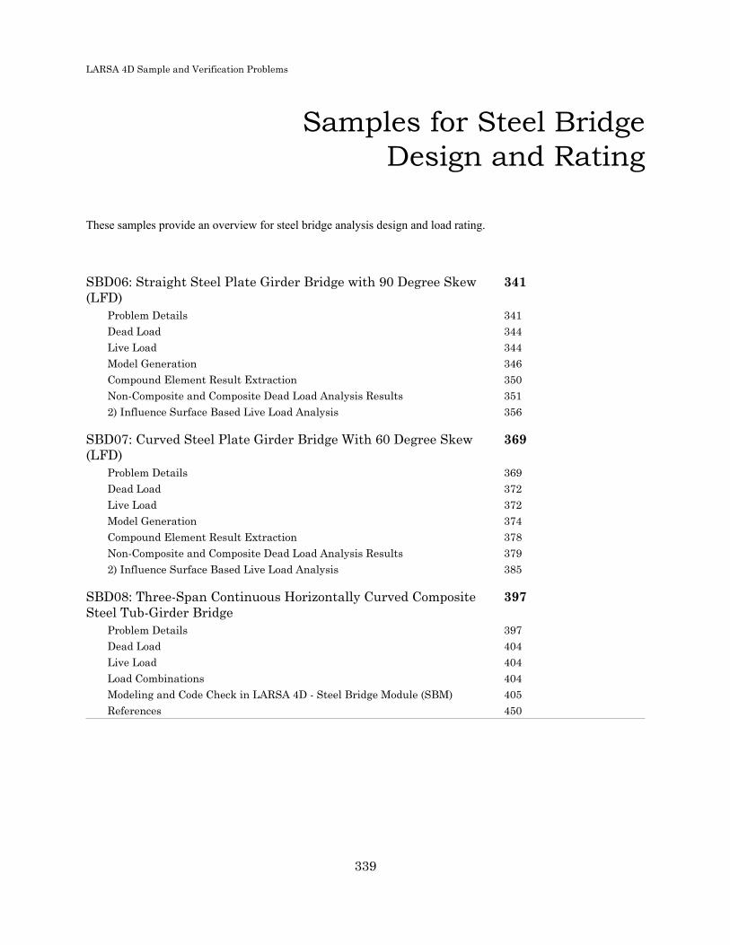
LARSA 4D Sample and Verification Problems
Samples for Steel BridgeDesign and Rating
These samples provide an overview for steel bridge analysis design and load rating.
SBD06: Straight Steel Plate Girder Bridge with 90 Degree Skew(LFD)
341
Problem Details 341Dead Load 344Live Load 344Model Generation 346Compound Element Result Extraction 350Non-Composite and Composite Dead Load Analysis Results 3512) Influence Surface Based Live Load Analysis 356
SBD07: Curved Steel Plate Girder Bridge With 60 Degree Skew(LFD)
369
Problem Details 369Dead Load 372Live Load 372Model Generation 374Compound Element Result Extraction 378Non-Composite and Composite Dead Load Analysis Results 3792) Influence Surface Based Live Load Analysis 385
SBD08: Three-Span Continuous Horizontally Curved CompositeSteel Tub-Girder Bridge
397
Problem Details 397Dead Load 404Live Load 404Load Combinations 404Modeling and Code Check in LARSA 4D - Steel Bridge Module (SBM) 405References 450
339

LARSA 4D Sample and Verification Problems
340

LARSA 4D Sample and Verification Problems
SBD06: Straight Steel Plate GirderBridge with 90 Degree Skew (LFD)
The bridge chosen for this example is a straight two-lane steel plate girder bridge with a 90-degree skew and withidentical four-girder cross-sections. The bridge is three-span continuous over span lengths of 80, 100 and 80 feet alongthe control centerline. The live load results are reported for HS25-44 and lane loading using influence surface analysis.
Example Project: The example described here can be found in the Steel Bridge Module folder of your LARSA 4DSamples directory (generally My Documents\LARSA Projects\Samples) in the file SBD06.
Problem DetailsThe bridge layout is shown in Figure 1.
Figure 1: Plan View
The materials used in this model are:
Steel
Es = 29,000 ksi
Weight Density = 490 pcf
Steel Girders = Type A572 Steel
Cross-Frames = Type A36 Steel
Concrete
Ec = 3,820 ksi
Weight Density = 150 pcf (which includes allowance for steel reinforcement)
fc' = 4.5 ksi
n = 8
341
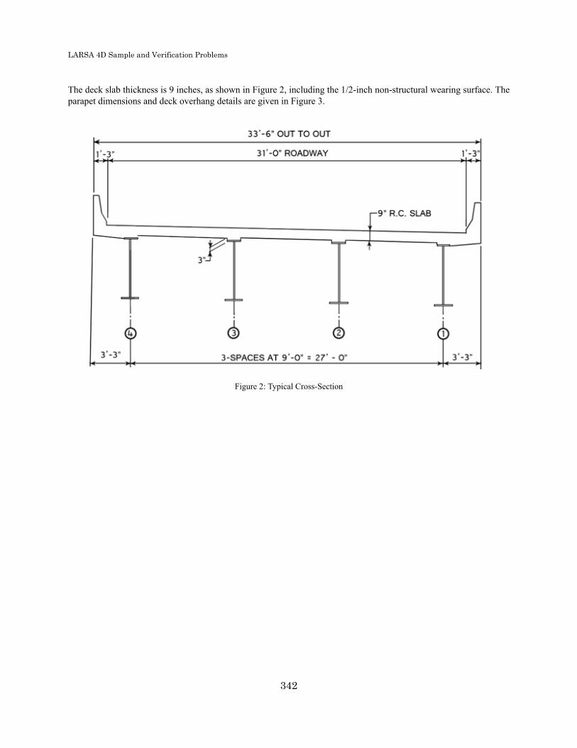
LARSA 4D Sample and Verification Problems
The deck slab thickness is 9 inches, as shown in Figure 2, including the 1/2-inch non-structural wearing surface. Theparapet dimensions and deck overhang details are given in Figure 3.
Figure 2: Typical Cross-Section
342
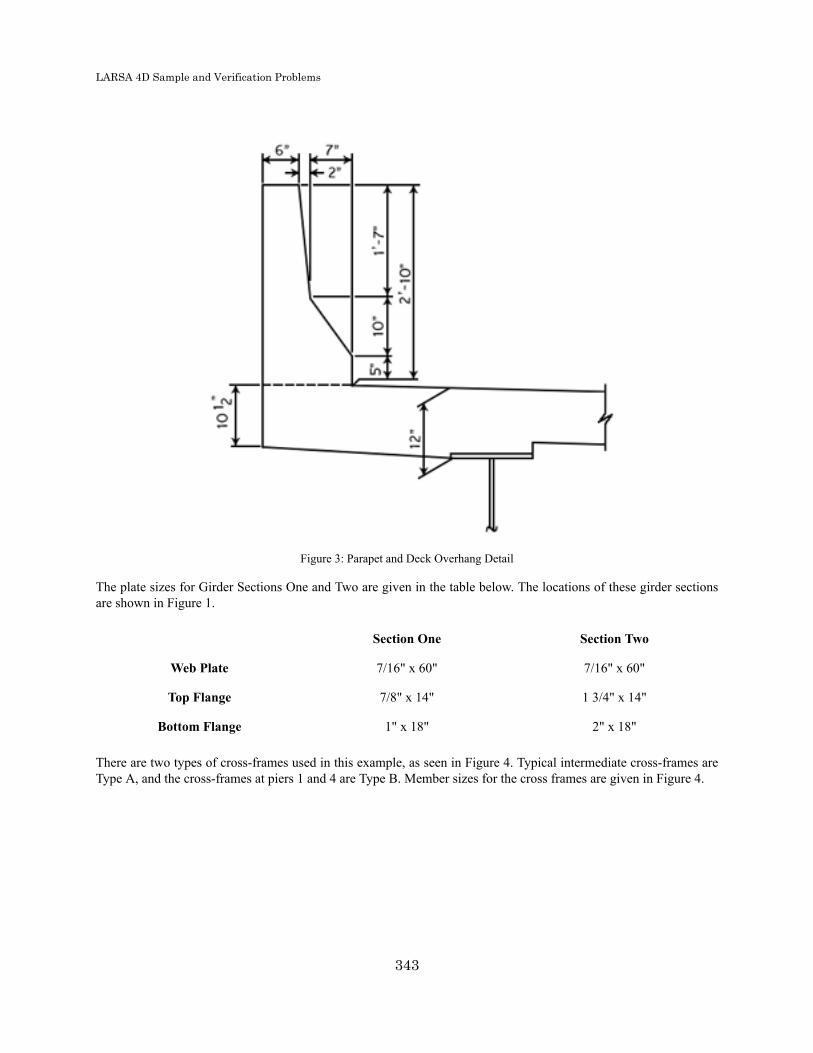
LARSA 4D Sample and Verification Problems
Figure 3: Parapet and Deck Overhang Detail
The plate sizes for Girder Sections One and Two are given in the table below. The locations of these girder sectionsare shown in Figure 1.
Section One Section Two
Web Plate 7/16" x 60" 7/16" x 60"
Top Flange 7/8" x 14" 1 3/4" x 14"
Bottom Flange 1" x 18" 2" x 18"
There are two types of cross-frames used in this example, as seen in Figure 4. Typical intermediate cross-frames areType A, and the cross-frames at piers 1 and 4 are Type B. Member sizes for the cross frames are given in Figure 4.
343

LARSA 4D Sample and Verification Problems
Figure 4: Cross-Frames
Dead LoadThe non-composite dead load consists of all of the dead loads, except the weight of the parapet and future wearingsurface. The composite dead load includes all of the dead loads.
The stay-in-place forms are 15 psf and are used between the girders, but not on the overhangs.
The future wearing surface is 30 psf and placed between the parapets.
Live LoadThe live load consists of a HS25-44 truck, as shown in the figure below, and distributed lane loading.
344
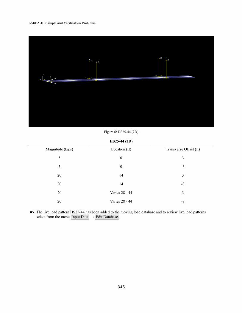
LARSA 4D Sample and Verification Problems
Figure 6: HS25-44 (2D)
HS25-44 (2D)
Magnitude (kips) Location (ft) Transverse Offset (ft)
5 0 3
5 0 -3
20 14 3
20 14 -3
20 Varies 28 - 44 3
20 Varies 28 - 44 -3
The live load pattern HS25-44 has been added to the moving load database and to review live load patternsselect from the menu Input Data → Edit Database .
345

LARSA 4D Sample and Verification Problems
Figure 7:Moving Load Database
Model GenerationThe model is created using the Steel Bridge Module within LARSA 4D BRIDGE. While this model could have beencreated using the graphical generation tools of LARSA 4D, the Steel Bridge Module provides a parametric approachfor fast-track generation of LARSA 4D models for I, box, and tub girder steel bridges and for performing AASHTOLRFD code check and load rating on these bridges. The module is specifically developed for the special needs ofskewed and/or curved bridges and bridge structures with complex geometry.
Steel I-girder sections can be represented as a single beam element or as multi-element section where the flanges arerepresented as beam elements and the web as shell elements. In this example, we will have I-girders modeled using acombination of member and shell elements. This modeling type allows easier extraction of lateral bending moments ofthe flanges. The top flange of the girder will be connected to the deck with rigid elements. The bridge deck is modeledusing shell elements.
The model generated is for staged construction analysis where non-composite and composite states and the deckpouring sequence are handled with ease.
The finite element model generated is displayed below.
346

LARSA 4D Sample and Verification Problems
Figure 8: LARSA 4D Finite Element Model
In the first stage, girders and cross frames are constructed as seen in Figure 9.
Figure 9: Stage 1-Girders and Cross Frames
347

LARSA 4D Sample and Verification Problems
In the second stage, stay-in-place form loads are applied to the girders as seen in Figure 10.
Figure 10: Stage 2-Stay in place form loads
In the third stage, the deck is poured and wet concrete loading is applied to the girders as seen in Figure 11.
Figure 11: Stage 3-Deck Pouring
In the fourth stage, the deck gained its stiffness and deck elements are constructed with LARSA 4D's stiffness onlyoption.
348
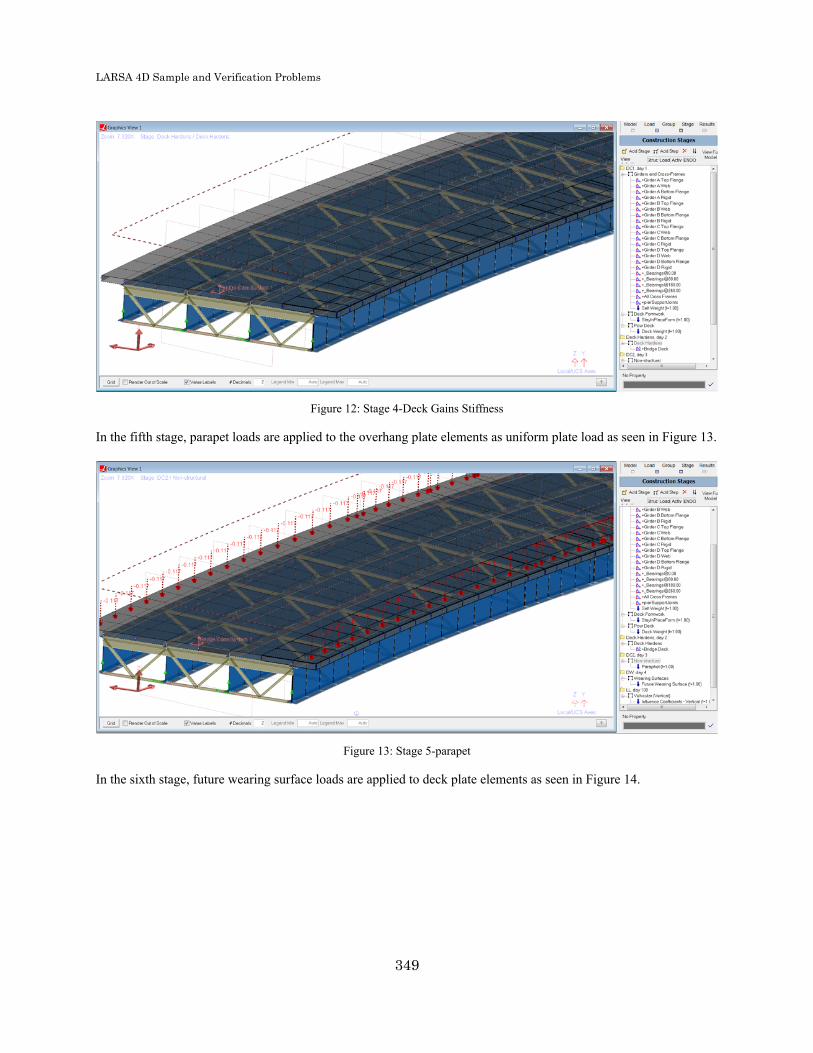
LARSA 4D Sample and Verification Problems
Figure 12: Stage 4-Deck Gains Stiffness
In the fifth stage, parapet loads are applied to the overhang plate elements as uniform plate load as seen in Figure 13.
Figure 13: Stage 5-parapet
In the sixth stage, future wearing surface loads are applied to deck plate elements as seen in Figure 14.
349

LARSA 4D Sample and Verification Problems
Figure 14: Stage 6-Future Wearing Surface
Modular ratio values of "n" and "3n" will be used by defining a material time effect as seen in Figure 15. In the seventhstage, the stiffness of the deck will be modified for the analysis of live load.
Figure 15: Stage 7-Influence Surface Analysis
Compound Element Result ExtractionIn order to determine the forces in a girder modeled not as a single beam but as multiple elements, the compoundelement forces feature of LARSA 4D shall be used. Compound Element Forces reports the combined forces andmoments of a group of elements about their combined centroid.
350

LARSA 4D Sample and Verification Problems
Non-Composite and Composite Dead Load Analysis ResultsThe non-composite dead load consists of all of the dead loads, except the weight of parapet and future wearing surface.The composite dead load includes all dead loads.
Deck weight is applied to the exterior girders as uniform member loads with a magnitude of 1.007 kips/ft.
Deck weight is applied to the interior girders as uniform member loads with a magnitude of 1.056 kips/ft.
Stay-in-place form loading is applied to the exterior girders as uniform member loads with a magnitude of 0.0675kips/ft.
Stay-in-place form loading is applied to the interior girders as uniform member loads with a magnitude of 0.135 kips/ft.
Follow the instructions below to review the loads.
To see load spreadsheets, click the Loads button above the explorers, right-click the StayInPlaceForm loadcase and choose Edit loads .
To see loads graphically, choose from the menu Graphics → Show and turn on Input Loads . Click theLoads button above the explorers, then click the StayInPlaceForm load case.
The non-composite dead load analysis results for the Girder 3 can be seen in Figure 16.Follow the steps below in order to see the results for Girder 3.
Select the structure group: Click the Group button above the explorers. Click Composite 2 . Click Select(Unselect Everything Else) .
Select the result case: Click the Results above the explorers. Right click the NonComposite result case.Choose Compound Element Forces .
Figure 16: Girder 3 Non-composite Dead Load Bending Moment
351
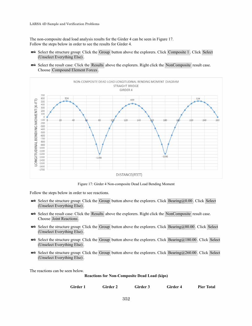
LARSA 4D Sample and Verification Problems
The non-composite dead load analysis results for the Girder 4 can be seen in Figure 17.Follow the steps below in order to see the results for Girder 4.
Select the structure group: Click the Group button above the explorers. Click Composite 1 . Click Select(Unselect Everything Else) .
Select the result case: Click the Results above the explorers. Right click the NonComposite result case.Choose Compound Element Forces .
Figure 17: Girder 4 Non-composite Dead Load Bending Moment
Follow the steps below in order to see reactions.
Select the structure group: Click the Group button above the explorers. Click [email protected] . Click Select(Unselect Everything Else) .
Select the result case: Click the Results above the explorers. Right click the NonComposite result case.Choose Joint Reactions .
Select the structure group: Click the Group button above the explorers. Click [email protected] . Click Select(Unselect Everything Else) .
Select the structure group: Click the Group button above the explorers. Click [email protected] . Click Select(Unselect Everything Else) .
Select the structure group: Click the Group button above the explorers. Click [email protected] . Click Select(Unselect Everything Else) .
The reactions can be seen below.Reactions for Non-Composite Dead Load (kips)
Girder 1 Girder 2 Girder 3 Girder 4 Pier Total
352
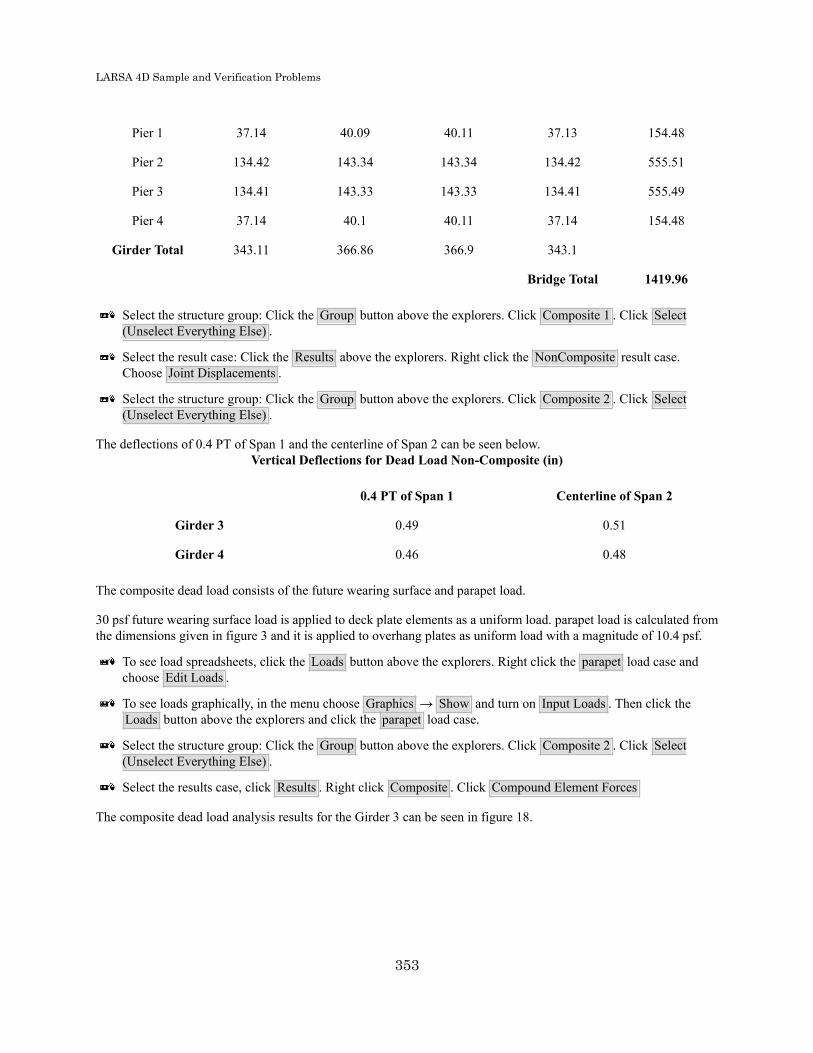
LARSA 4D Sample and Verification Problems
Pier 1 37.14 40.09 40.11 37.13 154.48
Pier 2 134.42 143.34 143.34 134.42 555.51
Pier 3 134.41 143.33 143.33 134.41 555.49
Pier 4 37.14 40.1 40.11 37.14 154.48
Girder Total 343.11 366.86 366.9 343.1
Bridge Total 1419.96
Select the structure group: Click the Group button above the explorers. Click Composite 1 . Click Select(Unselect Everything Else) .
Select the result case: Click the Results above the explorers. Right click the NonComposite result case.Choose Joint Displacements .
Select the structure group: Click the Group button above the explorers. Click Composite 2 . Click Select(Unselect Everything Else) .
The deflections of 0.4 PT of Span 1 and the centerline of Span 2 can be seen below.Vertical Deflections for Dead Load Non-Composite (in)
0.4 PT of Span 1 Centerline of Span 2
Girder 3 0.49 0.51
Girder 4 0.46 0.48
The composite dead load consists of the future wearing surface and parapet load.
30 psf future wearing surface load is applied to deck plate elements as a uniform load. parapet load is calculated fromthe dimensions given in figure 3 and it is applied to overhang plates as uniform load with a magnitude of 10.4 psf.
To see load spreadsheets, click the Loads button above the explorers. Right click the parapet load case andchoose Edit Loads .
To see loads graphically, in the menu choose Graphics → Show and turn on Input Loads . Then click theLoads button above the explorers and click the parapet load case.
Select the structure group: Click the Group button above the explorers. Click Composite 2 . Click Select(Unselect Everything Else) .
Select the results case, click Results . Right click Composite . Click Compound Element Forces
The composite dead load analysis results for the Girder 3 can be seen in figure 18.
353
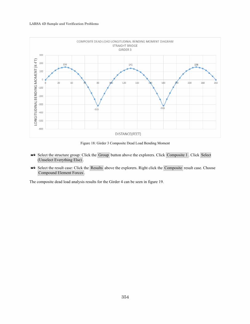
LARSA 4D Sample and Verification Problems
Figure 18: Girder 3 Composite Dead Load Bending Moment
Select the structure group: Click the Group button above the explorers. Click Composite 1 . Click Select(Unselect Everything Else) .
Select the result case: Click the Results above the explorers. Right click the Composite result case. ChooseCompound Element Forces .
The composite dead load analysis results for the Girder 4 can be seen in figure 19.
354

LARSA 4D Sample and Verification Problems
Figure 19: Girder 4 Composite Dead Load Bending Moment
The reactions can be seen below.
Select the structure group: Click the Group button above the explorers. Click [email protected] . Click Select(Unselect Everything Else) .
Select the result case: Click the Results above the explorers. Right click the Composite result case. ChooseJoint Reactions .
Select the structure group: Click the Group button above the explorers. Click [email protected] . Click Select(Unselect Everything Else) .
Select the structure group: Click the Group button above the explorers. Click [email protected] . Click Select(Unselect Everything Else) .
Select the structure group: Click the Group button above the explorers. Click [email protected] . Click Select(Unselect Everything Else) .
Vertical Reactions Composite Dead Load (kips)
Girder 1 Girder 2 Girder 3 Girder 4 Pier Total
Pier 1 14.17 9.06 9.04 14.18 46.45
Pier 2 48.47 32.7 32.7 48.46 162.33
Pier 3 48.47 32.7 32.7 48.46 162.33
Pier 4 14.17 9.06 9.04 14.18 46.45
Girder Total 125.27 83.52 83.49 125.28
Bridge Total 417.56
355

LARSA 4D Sample and Verification Problems
The deflections of 0.4 PT of Span 1 and the centerline of Span 2 can be seen below
Select the structure group: Click the Group button above the explorers. Click Composite 1 . Click Select(Unselect Everything Else) .
Select the result case: Click the Results above the explorers. Right click the Composite result case. ChooseJoint Displacements .
Select the structure group: Click the Group button above the explorers. Click Composite 2 . Click Select(Unselect Everything Else) .
Vertical Deflections Composite Dead Load (in)
0.4 PT of Span 1 Centerline of Span 2
Girder 3 0.069 0.083
Girder 4 0.086 0.099
2) Influence Surface Based Live Load Analysis2.1) Live Load Definitions
HS25-44 truck and lane loading will be applied according to AASHTO LFD. We will use the influence surface basedresult cases in LARSA 4D for simulating following conditions.
1 - HS25-44 Truck Only
2 - For Positive Moment: Concentrated Load (22.5 Kips) + Lane (0.8 kips/ft)
3 - For Negative Moment: Concentrated Load Pair (2 x 22.5 Kips) + Lane (0.8 kips/ft)
4 - For Shear: Concentrated Load (32.5 Kips) + Lane (0.8 kips/ft)
LARSA4D will find the worst case live load positioning for the result cases using the conditions above.
2.2) Influence Surface Result Case Settings
Influence based result case definition consists of general loading parameters, vehicular loading options and uniform/patch loading options.
General loading parameters include design lane width, overall factor and multiple presence factors along withother options. The overall factor defined on General Options parameters tab applies to both vehicular and laneloading.However the factor defined in vehicular tab applies to vehicle loads only.
General options for influence surface result cases will be defined as shown in figure 21.
The design lane width is 12 feet.
Multiple presence factors are 1.00 for 1 lane and 2 lanes loaded, 0.90 for 3 lanes loaded, and 0.75 for 4 or more lanesloaded.Overall factor is entered as 1.232 and detailed explanation is below.
356

LARSA 4D Sample and Verification Problems
Figure 21: General Settings of Influence Surface Result Case
LARSA 4D provides the ability for the user to enter different impact factors for every span as longitudinal factors.In our example for 80 feet span, the impact factor is calculated as 0.244 " Impact = 50 / ( L + 125) " where L = 80feet(span length) and for 100 feet span, impact factor is calculated as 0.222 " Impact = 50 / ( L + 125) " where L= 100 feet(span length). These factors can be entered as the longitudinal factors using the stations along the controlcenterline as in figure 22.
Figure 22: Impact factors as longitudinal factors
357

LARSA 4D Sample and Verification Problems
In this example the variation of impact factors is less than 1% and for simplicity it will be ignored. An average 90 feetspan length is used in impact factor calculation and it is calculated as 0.232. Overall factor is entered as 1.232 (1.00+ Impact factor) for all influence surface cases as seen in figure 21.
In LFD, the impact factor is applied to the entire live load. In LRFD, dynamic load allowance is applied only to thedesign truck and design tandem. For this reason LARSA4D has options for entering different live load factors forvehicles and lane loading. The overall factor entered in General Options tab is for entire live load and suitable for LFDloading. Factor entered in Vehicular Loading tab is applied to the vehicle only (doesn't effect the lane loading), andit is suitable for LRFD loading.Vehicle loading factor is entered as 1.00 for all 4 cases. UDL factor is entered as 0.00 for HS25-44 truck only casesince the AASHTO LFD doesn't require the lane loading and truck loading together. For the remaining 3 cases, UDLfactor is entered as 1.
The design lane vehicle margin is entered as 2 feet.
Vehicular Loading tabs for all 4 cases can be seen in Figure 23.
358

LARSA 4D Sample and Verification Problems
Figure 23: LARSA 4D Influence Result Case
359

LARSA 4D Sample and Verification Problems
UDL load magnitude is entered as 0.8 kip/ft along with UDL width per design lane as 10 ft according to AASHTOLFD and a screenshot from LARSA 4D can be seen in the figure 24.
Figure 24: Lane Load Settings of Influence Surface Result Case
Follow the steps below in order to view influence surface result case settings shown above.
Select the result case: Click the Results above the explorers. Right click the HS25-44 result case. ChooseProperties .
Select the result case: Click the Results above the explorers. Right click the Concentrated Load (22.5 Kips)result case. Choose Properties .
Select the result case: Click the Results above the explorers. Right click the Concentrated Load (32.5 Kips) +Lane (0.8 kips/ft) result case. Choose Properties .
Select the result case: Click the Results above the explorers. Right click the Concentrated Load Pair (22.5 Kips)+ Lane (0.8 kips/ft) result case. Choose Properties .
2.3)Live Load Analysis Results
In order to see the force effect on each girder, LARSA 4D's compound element force tool will be used. Compoundelement forces report the combined forces and moments of a group of elements regards to their combined centroid.These results are used to determine the forces in a girder modeled not as a single beam but as a group of elements.Since our deck is modeled with plate elements and the girder with beam and plate elements, the compound elementforces tool will be used to find the forces for composite section. With the help of this tool,the user can see the forceeffects on each girder directly.
Thus AASHTO Section 3, Part C, Distribution of Loads is not applicable for this type of refined modelling thereforethe results reported do not require girder distribution factors to be used.
In this example, we will be using extreme effect groups to extract envelope of forces. Extreme effect groups representthe worst-case scenario from a set of result cases, similar to envelopes, but are saved as new result cases. For positive
360

LARSA 4D Sample and Verification Problems
moment, extreme effect group named 'Positive Moment' is created and includes result cases corresponding truck alone(HS25-44) and lane load for positive moment (Concentrated Load (22.5 Kips) + Lane).
Figure 25: Extreme Effect Group For Positive Moment
For negative moment, extreme effect group named "Negative Moment" is created and includes result casescorresponding truck alone (HS25-44) and lane load for negative moment (Concentrated Load Pair (22.5 Kips) + Lane).
Figure 26: Extreme Effect Group For Negative Moment
For shear , extreme effect group named "Shear" is created and includes result cases corresponding truck alone(HS25-44) and lane load for shear (Concentrated Load (32.5 Kips) + Lane).
361

LARSA 4D Sample and Verification Problems
Figure 27: Extreme Effect Group For Shear
Bending moment results for girder 3 is shown in figure 28.Follow the steps below in order to see bending moment results for Girder 3.
Select the structure group: Click the Group button above the explorers. Click Composite 2 . click Select(Unselect Everything Else) .
Select the result case: Click the Results above the explorers. Right click the Positive Moment result case. ChooseCompound Element Forces .
Select Envelope Max My
Select the result case: Click the Results above the explorers. Right click the Negative Moment result case.Choose Compound Element Forces .
Select Envelope Min My
362
LARSA 4D Sample and Verification Problems
Figure 28: Girder 3 Bending Moment
Bending moment results for girder 4 is shown in figure 29. Follow the steps below in order to see bending momentresults for Girder 4.
Select the structure group: Click the Group button above the explorers. Click Composite 1 . click Select(Unselect Everything Else) .
Select the result case: Click the Results above the explorers. Right click the Positive Moment result case. ChooseCompound Element Forces .
Select Envelope Max My363

LARSA 4D Sample and Verification Problems
Select the result case: Click the Results above the explorers. Right click the Negative Moment result case.Choose Compound Element Forces .
Select Envelope Min My
Figure 29: Girder 4 Bending Moment
Critical reactions at supports are tabulated below. Follow the steps below in order to display live load reaction forces.
Select the structure group: Click the Group button above the explorers. Click [email protected] . click Select(Unselect Everything Else) .
364

LARSA 4D Sample and Verification Problems
Select the result case: Click the Results above the explorers. Right click the Shear result case. Choose JointReactions .
Select Envelope Max Fz
Select the structure group: Click the Group button above the explorers. Click [email protected] . click Select(Unselect Everything Else) .
Select the structure group: Click the Group button above the explorers. Click [email protected] . click Select(Unselect Everything Else) .
Select the structure group: Click the Group button above the explorers. Click [email protected] . click Select(Unselect Everything Else) .
Live Load Vertical Reactions (kips)
Girder 1 Girder 2 Girder 3 Girder 4
Pier 1 68.29 86.51 86.51 68.08
Pier 2 118.91 138.53 138.41 118.42
Pier 3 115.54 137.98 137.87 114.99
Pier 4 68.32 84.36 84.20 68.03
The maximum tensile and compressive forces for the cross-frames at the center of span 2 between girder 2 and 3 aretabulated below.Follow the steps below in order to see axial force for live load.
Select the structure group: Click the Group button above the explorers. Click _Cross-frame G3-G2@130 .click Select (Unselect Everything Else) .
Select all 3 result cases: Click the Results above the explorers. Right click the Positive Moment result case.Choose Member Sectional Forces . Press CTRL on the keyboard and click Negative Moment , Shear resultcases.
Select Envelope FxCross Frame Axial Force At Center Of Span 2 Between Girder 2-3 Due to Live Load (kips)
Bottom Chord Diagonals
Tension 7.57 16.49
Compression -5.51 -11.29
Bottom flange lateral moments for girder 3 and 4 can be seen below.Bottom Flange Lateral Moment Due to Live Load (kips.ft)
Pier 2 Center of Span 2
Girder 3 3.39 1.71
Girder 4 3.97 2.21
365

LARSA 4D Sample and Verification Problems
Select the structure group: Click the Group button above the explorers. Click Girder B Bottom Flange . ClickSelect (Unselect Everything Else) .
Select all 3 result cases: Click the Results above the explorers. Right click the Positive Moment result case.Choose Member Sectional Forces . Press CTRL on the keyboard and click Negative Moment , Shear resultcases.
Select Envelope My
Figure 30: Girder 3 Bottom Flange Lateral Moments
Select the structure group: Click the Group button above the explorers. Click Girder A Bottom Flange . ClickSelect (Unselect Everything Else) .
Select all 3 result cases: Click the Results above the explorers. Right click the Positive Moment result case.Choose Member Sectional Forces . Press CTRL on the keyboard and click Negative Moment , Shear resultcases.
Select Envelope My
366

LARSA 4D Sample and Verification Problems
Figure 31: Girder 4 Bottom Flange Lateral Moments
367

LARSA 4D Sample and Verification Problems
368

LARSA 4D Sample and Verification Problems
SBD07: Curved Steel Plate GirderBridge With 60 Degree Skew (LFD)
Featuring a 60 degree skew, the bridge chosen for this example is a two-lane steel plate girder bridge with identicalfour-girder cross-sections. This curved bridge, featuring a 500 feet radius, is three-span continuous over span lengthsof 80, 100, and 80 feet, along the control centerline. The live load results are reported for HS25-44 and lane loadingusing influence surface analysis.
Example Project: The example described here can be found in the Steel Bridge Module folder of your LARSA 4DSamples directory (generally My Documents\LARSA Projects\Samples) in the file SBD07.
Problem DetailsThe bridge layout is shown in Figure 1.
Figure 1: Plan View
The materials used in this model are:
Steel
Es = 29,000 ksi
Weight Density = 490 pcf
Steel Girders = Type A572 Steel
Cross-Frames = Type A36 Steel
369

LARSA 4D Sample and Verification Problems
Concrete
Ec = 3,820 ksi
Weight Density = 150 pcf (which includes allowance for steel reinforcement)
fc' = 4.5 ksi
n = 8
The deck slab thickness is 9 inches, as shown in Figure 2, including the 1/2-inch non-structural wearing surface. Theparapet dimensions and deck overhang details are given in Figure 3.
Figure 2: Typical Cross-Section
370

LARSA 4D Sample and Verification Problems
Figure 3: Parapet and Deck Overhang Detail
The plate sizes for Girder Sections One and Two are given in the table below. The locations of these girder sectionsare shown in Figure 1.
Section One Section Two
Web Plate 7/16" x 60" 7/16" x 60"
Top Flange 7/8" x 14" 1 3/4" x 14"
Bottom Flange 1" x 18" 2" x 18"
There are two types of cross-frames used in this example, as seen in Figure 4. Typical intermediate cross-frames areType A, and the cross-frames at piers 1 and 4 are Type B. Member sizes for the cross frames are given in Figure 4.
371

LARSA 4D Sample and Verification Problems
Figure 4: Cross-Frames
Dead LoadThe non-composite dead load consists of all of the dead loads, except the weight of the parapet and future wearingsurface. The composite dead load includes all of the dead loads.
The stay-in-place forms are 15 psf and are used between the girders, but not on the overhangs.
The future wearing surface is 30 psf and placed between the parapets.
Live LoadThe live load consists of a HS25-44 truck, as shown in the figure below, and distributed lane loading.
372

LARSA 4D Sample and Verification Problems
Figure 6: HS25-44 (2D)
HS25-44 (2D)
Magnitude (kips) Location (ft) Transverse Offset (ft)
5 0 3
5 0 -3
20 14 3
20 14 -3
20 Varies 28 - 44 3
20 Varies 28 - 44 -3
The live load pattern HS25-44 has been added to the moving load database and to review live load patternsselect from the menu Input Data → Edit Database .
373

LARSA 4D Sample and Verification Problems
Figure 7:Moving Load Database
Model GenerationThe model is created using the Steel Bridge Module within LARSA 4D BRIDGE. While this model could have beencreated using the graphical generation tools of LARSA 4D, the Steel Bridge Module provides a parametric approachfor fast-track generation of LARSA 4D models for I, box, and tub girder steel bridges and for performing AASHTOLRFD code check and load rating on these bridges. The module is specifically developed for the special needs ofskewed and/or curved bridges and bridge structures with complex geometry.
Steel I-girder sections can be represented as a single beam element or as multi-element section where the flanges arerepresented as beam elements and the web as shell elements. In this example, we will have I-girders modeled using acombination of member and shell elements. This modeling type allows easier extraction of lateral bending moments ofthe flanges. The top flange of the girder will be connected to the deck with rigid elements. The bridge deck is modeledusing shell elements.
The model generated is for staged construction analysis where non-composite and composite states, deck pouringsequences are handled with ease.
The finite element model generated is displayed below.
374

LARSA 4D Sample and Verification Problems
Figure 8: LARSA 4D Finite Element Model
In the first stage, girders and cross frames are constructed as seen in Figure 9.
Figure 9: Stage 1-Girders and Cross Frames
In the second stage, stay-in-place form loads are applied to the girders as seen in Figure 10.
375

LARSA 4D Sample and Verification Problems
Figure 10: Stage 2-Stay in place form loads
In the third stage, the deck is poured and wet concrete loading is applied to the girders as seen in Figure 11.
Figure 11: Stage 3-Deck Pouring
In the fourth stage, the deck gained its stiffness and deck elements are constructed with LARSA 4D's stiffness onlyoption.
376

LARSA 4D Sample and Verification Problems
Figure 12: Stage 4-Deck Gains Stiffness
In the fifth stage, parapet loads are applied to the overhang plate elements as uniform plate load as seen in Figure 13.
Figure 13: Stage 5-parapet
In the sixth stage, future wearing surface loads are applied to deck plate elements as seen in Figure 14.
377

LARSA 4D Sample and Verification Problems
Figure 14: Stage 6-Future Wearing Surface
Modular ratio values of "n" and "3n" will be used by defining a material time effect as seen in Figure 15. In the seventhstage, the stiffness of the deck will be modified for the analysis of live load.
Figure 15: Stage 7-Influence Surface Analysis
Compound Element Result ExtractionIn order to determine the forces in a girder modeled not as a single beam but as multiple elements, the compoundelement forces feature of LARSA 4D shall be used. Compound Element Forces reports the combined forces andmoments of a group of elements about their combined centroid.
378

LARSA 4D Sample and Verification Problems
Non-Composite and Composite Dead Load Analysis ResultsThe non-composite dead load consists of all of the dead loads, except the weight of parapet and future wearing surface.The composite dead load includes all dead loads.
Deck weight is applied to the exterior girders as uniform member loads with a magnitude of 1.007 kips/ft.
Deck weight is applied to the interior girders as uniform member loads with a magnitude of 1.056 kips/ft.
Stay-in-place form loading is applied to the exterior girders as uniform member loads with a magnitude of 0.0675kips/ft.
Stay-in-place form loading is applied to the interior girders as uniform member loads with a magnitude of 0.135 kips/ft.
Follow the instructions below to review the loads.
To see load spreadsheets, click the Loads button above the explorers, right-click the StayInPlaceForm loadcase and choose Edit loads .
To see loads graphically, choose from the menu Graphics → Show and turn on Input Loads . click the Loadsbutton above the explorers, then click the StayInPlaceForm load case.
The non-composite dead load analysis results for the Girder 3 can be seen in Figure 16.Follow the steps below in order to see the results for Girder 3.
Select the structure group: Click the Group button above the explorers. Click Composite 2 . Click Select(Unselect Everything Else) .
Select the result case: Click the Results above the explorers. Right click the NonComposite result case.Choose Compound Element Forces .
379

LARSA 4D Sample and Verification Problems
Figure 16: Girder 3 Non-composite Dead Load Bending Moment
The non-composite dead load analysis results for the Girder 4 can be seen in Figure 17.Follow the steps below in order to see the results for Girder 4.
Select the structure group: Click the Group button above the explorers. Click Composite 1 . Click Select(Unselect Everything Else) .
Select the result case: Click the Results above the explorers. Right click the NonComposite result case.Choose Compound Element Forces .
380

LARSA 4D Sample and Verification Problems
Figure 17: Girder 4 Non-composite Dead Load Bending Moment
Follow the steps below in order to see reactions.
Select the structure group: Click the Group button above the explorers. Click [email protected] . Click Select(Unselect Everything Else) .
Select the result case: Click the Results above the explorers. Right click the NonComposite result case.Choose Joint Reactions .
Select the structure group: Click the Group button above the explorers. Click [email protected] . Click Select(Unselect Everything Else) .
Select the structure group: Click the Group button above the explorers. Click [email protected] . Click Select(Unselect Everything Else) .
Select the structure group: Click the Group button above the explorers. Click [email protected] . Click Select(Unselect Everything Else) .
The reactions can be seen below.Reactions for Non-Composite Dead Load (kips)
Girder 1 Girder 2 Girder 3 Girder 4 Pier Total
Pier 1 33.76 40.29 39.28 40.05 153.38
Pier 2 140.22 138.36 151.63 129.67 559.88
Pier 3 139.98 138.32 149.82 127.83 555.95
Pier 4 35.15 39.70 40.86 39.57 155.28
381

LARSA 4D Sample and Verification Problems
Girder Total 349.12 356.67 381.59 337.11
Bridge Total 1424.49
Follow the steps below in order to see joint displacements for Girder 3 and 4.
Select the structure group: Click the Group button above the explorers. Click Composite 1 . Click Select(Unselect Everything Else) .
Select the result case: Click the Results above the explorers. Right click the NonComposite result case.Choose Joint Displacements .
Select the structure group: Click the Group button above the explorers. Click Composite 2 . Click Select(Unselect Everything Else) .
The deflections of 0.4 PT of Span 1 and the centerline of Span 2 can be seen below.Vertical Deflections for Dead Load Non-Composite (in)
0.4 PT of Span 1 Centerline of Span 2
Girder 3 0.49 0.50
Girder 4 0.51 0.49
The composite dead load consists of the future wearing surface and parapet load.
30 psf future wearing surface load is applied to deck plate elements as a uniform load. parapet load is calculated fromthe dimensions given in figure 3 and it is applied to overhang plates as uniform load with a magnitude of 10.4 psf.
To see load spreadsheets, click the Loads button above the explorers. Right click the parapet load case andchoose Edit Loads .
To see loads graphically, in the menu choose Graphics → Show and turn on Input Loads . Then click theLoads button above the explorers and click the parapet load case.
Follow the steps below in order to see results for Girder 3.
Select the structure group: Click the Group button above the explorers. Click Composite 2 . Click Select(Unselect Everything Else) .
Select the results case, click Results . Right click Composite . Click Compound Element ForcesThe composite dead load analysis results for the Girder 3 can be seen in figure 18.
382

LARSA 4D Sample and Verification Problems
Figure 18: Girder 3 Composite Dead Load Bending Moment
Follow the steps below in order to see results for Girder 4.
Select the structure group: Click the Group button above the explorers. Click Composite 1 . Click Select(Unselect Everything Else) .
Select the result case: Click the Results above the explorers. Right click the Composite result case. ChooseCompound Element Forces .
The composite dead load analysis results for the Girder 4 can be seen in figure 19.
383

LARSA 4D Sample and Verification Problems
Figure 19: Girder 4 Composite Dead Load Bending Moment
The reactions can be seen below.Follow the steps below in order to see reactions.
Select the structure group: Click the Group button above the explorers. Click [email protected] . Click Select(Unselect Everything Else) .
Select the result case: Click the Results above the explorers. Right click the Composite result case. ChooseJoint Reactions .
Select the structure group: Click the Group button above the explorers. Click [email protected] . Click Select(Unselect Everything Else) .
Select the structure group: Click the Group button above the explorers. Click [email protected] . Click Select(Unselect Everything Else) .
Select the structure group: Click the Group button above the explorers. Click [email protected] . Click Select(Unselect Everything Else) .
Vertical Reactions Composite Dead Load (kips)
Girder 1 Girder 2 Girder 3 Girder 4 Pier Total
Pier 1 12.89 9.19 9.26 14.84 46.19
Pier 2 46.98 33.80 35.06 46.92 162.76
Pier 3 47.85 33.97 34.66 45.68 162.15
Pier 4 14.49 9.80 8.05 14.17 46.52
Girder Total 122.20 86.77 87.03 121.61
384
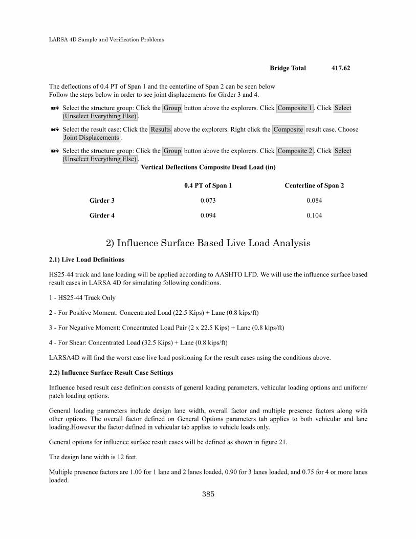
LARSA 4D Sample and Verification Problems
Bridge Total 417.62
The deflections of 0.4 PT of Span 1 and the centerline of Span 2 can be seen belowFollow the steps below in order to see joint displacements for Girder 3 and 4.
Select the structure group: Click the Group button above the explorers. Click Composite 1 . Click Select(Unselect Everything Else) .
Select the result case: Click the Results above the explorers. Right click the Composite result case. ChooseJoint Displacements .
Select the structure group: Click the Group button above the explorers. Click Composite 2 . Click Select(Unselect Everything Else) .
Vertical Deflections Composite Dead Load (in)
0.4 PT of Span 1 Centerline of Span 2
Girder 3 0.073 0.084
Girder 4 0.094 0.104
2) Influence Surface Based Live Load Analysis2.1) Live Load Definitions
HS25-44 truck and lane loading will be applied according to AASHTO LFD. We will use the influence surface basedresult cases in LARSA 4D for simulating following conditions.
1 - HS25-44 Truck Only
2 - For Positive Moment: Concentrated Load (22.5 Kips) + Lane (0.8 kips/ft)
3 - For Negative Moment: Concentrated Load Pair (2 x 22.5 Kips) + Lane (0.8 kips/ft)
4 - For Shear: Concentrated Load (32.5 Kips) + Lane (0.8 kips/ft)
LARSA4D will find the worst case live load positioning for the result cases using the conditions above.
2.2) Influence Surface Result Case Settings
Influence based result case definition consists of general loading parameters, vehicular loading options and uniform/patch loading options.
General loading parameters include design lane width, overall factor and multiple presence factors along withother options. The overall factor defined on General Options parameters tab applies to both vehicular and laneloading.However the factor defined in vehicular tab applies to vehicle loads only.
General options for influence surface result cases will be defined as shown in figure 21.
The design lane width is 12 feet.
Multiple presence factors are 1.00 for 1 lane and 2 lanes loaded, 0.90 for 3 lanes loaded, and 0.75 for 4 or more lanesloaded.
385

LARSA 4D Sample and Verification Problems
Overall factor is entered as 1.232 and detailed explanation is below.
Figure 21: General Settings of Influence Surface Result Case
LARSA 4D provides the ability for the user to enter different impact factors for every span as longitudinal factors.In our example for 80 feet span, the impact factor is calculated as 0.244 " Impact = 50 / ( L + 125) " where L = 80feet(span length) and for 100 feet span, impact factor is calculated as 0.222 " Impact = 50 / ( L + 125) " where L= 100 feet(span length). These factors can be entered as the longitudinal factors using the stations along the controlcenterline as in figure 22.
Figure 22: Impact factors as longitudinal factors
386

LARSA 4D Sample and Verification Problems
In this example the variation of impact factors is less than 1% and for simplicity it will be ignored. An average 90 feetspan length is used in impact factor calculation and it is calculated as 0.232. Overall factor is entered as 1.232 (1.00+ Impact factor) for all influence surface cases as seen in figure 21.
In LFD, the impact factor is applied to the entire live load. In LRFD, dynamic load allowance is applied only to thedesign truck and design tandem. For this reason LARSA4D has options for entering different live load factors forvehicles and lane loading. The overall factor entered in General Options tab is for entire live load and suitable for LFDloading. Factor entered in Vehicular Loading tab is applied to the vehicle only (doesn't effect the lane loading), andit is suitable for LRFD loading.
Vehicle loading factor is entered as 1.00 for all 4 cases. UDL factor is entered as 0.00 for HS25-44 truck only casesince the AASHTO LFD doesn't require the lane loading and truck loading together. For the remaining 3 cases, UDLfactor is entered as 1.
The design lane vehicle margin is entered as 2 feet.
Vehicular Loading tabs for all 4 cases can be seen in Figure 23.
387
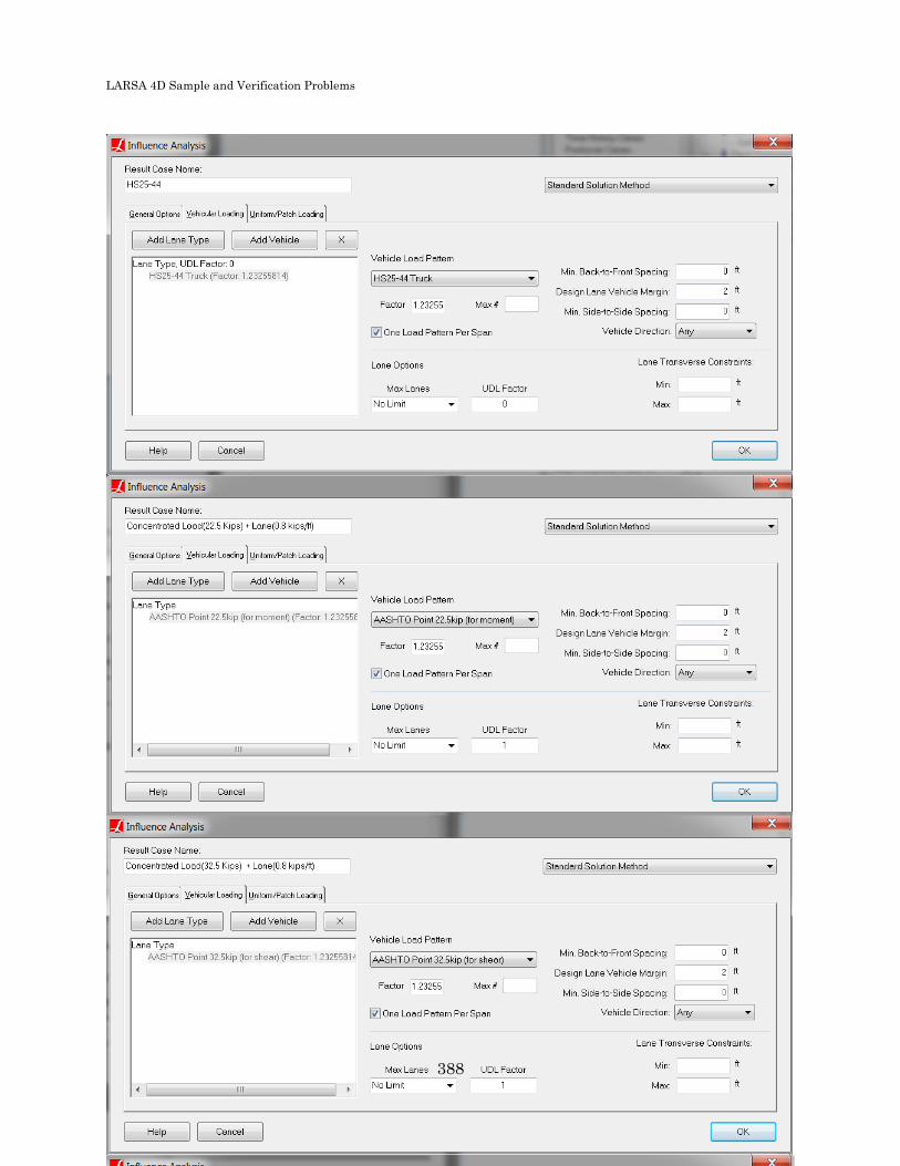
LARSA 4D Sample and Verification Problems
Figure 23: LARSA 4D Influence Result Case
388

LARSA 4D Sample and Verification Problems
UDL load magnitude is entered as 0.8 kip/ft along with UDL width per design lane as 10 ft according to AASHTOLFD and a screenshot from LARSA 4D can be seen in the figure 24.
Figure 24: Lane Load Settings of Influence Surface Result Case
Follow the steps below in order to view influence surface result case settings shown above.
Select the result case: Click the Results above the explorers. Right click the HS25-44 result case. ChooseProperties .
Select the result case: Click the Results above the explorers. Right click the Concentrated Load (22.5 Kips)result case. Choose Properties .
Select the result case: Click the Results above the explorers. Right click the Concentrated Load (32.5 Kips) +Lane (0.8 kips/ft) result case. Choose Properties .
Select the result case: Click the Results above the explorers. Right click the Concentrated Load Pair (22.5 Kips)+ Lane (0.8 kips/ft) result case. Choose Properties .
2.3)Live Load Analysis Results
In order to see the force effect on each girder, LARSA 4D's compound element force tool will be used. Compoundelement forces report the combined forces and moments of a group of elements regards to their combined centroid.These results are used to determine the forces in a girder modeled not as a single beam but as a group of elements.Since our deck is modeled with plate elements and the girder with beam and plate elements, the compound elementforces tool will be used to find the forces for composite section. With the help of this tool,the user can see the forceeffects on each girder directly.
Thus AASHTO Section 3, Part C, Distribution of Loads is not applicable for this type of refined modelling thereforethe results reported do not require girder distribution factors to be used.
In this example, we will be using extreme effect groups to extract envelope of forces. Extreme effect groups representthe worst-case scenario from a set of result cases, similar to envelopes, but are saved as new result cases. For positive
389

LARSA 4D Sample and Verification Problems
moment, extreme effect group named 'Positive Moment' is created and includes result cases corresponding truck alone(HS25-44) and lane load for positive moment (Concentrated Load (22.5 Kips) + Lane).
Figure 25: Extreme Effect Group For Positive Moment
For negative moment, extreme effect group named "Negative Moment" is created and includes result casescorresponding truck alone (HS25-44) and lane load for negative moment (Concentrated Load Pair (22.5 Kips) + Lane).
Figure 26: Extreme Effect Group For Negative Moment
For shear , extreme effect group named "Shear" is created and includes result cases corresponding truck alone(HS25-44) and lane load for shear (Concentrated Load (32.5 Kips) + Lane).
390

LARSA 4D Sample and Verification Problems
Figure 27: Extreme Effect Group For Shear
Bending moment results for girder 3 is shown in figure 28.Follow the steps below in order to see bending moment results for Girder 3.
Select the structure group: Click the Group button above the explorers. Click Composite 2 . click Select(Unselect Everything Else) .
Select the result case: Click the Results above the explorers. Right click the Positive Moment result case. ChooseCompound Element Forces .
Select Envelope Max My
Select the result case: Click the Results above the explorers. Right click the Negative Moment result case.Choose Compound Element Forces .
Select Envelope Min My
391
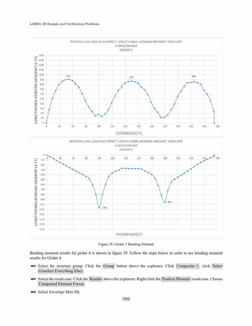
LARSA 4D Sample and Verification Problems
Figure 28: Girder 3 Bending Moment
Bending moment results for girder 4 is shown in figure 29. Follow the steps below in order to see bending momentresults for Girder 4.
Select the structure group: Click the Group button above the explorers. Click Composite 1 . click Select(Unselect Everything Else) .
Select the result case: Click the Results above the explorers. Right click the Positive Moment result case. ChooseCompound Element Forces .
Select Envelope Max My
392

LARSA 4D Sample and Verification Problems
Select the result case: Click the Results above the explorers. Right click the Negative Moment result case.Choose Compound Element Forces .
Select Envelope Min My
Figure 29: Girder 4 Bending Moment
Critical reactions at supports are tabulated below. Follow the steps below in order to display live load reaction forces.
Select the structure group: Click the Group button above the explorers. Click [email protected] . click Select(Unselect Everything Else) .
393

LARSA 4D Sample and Verification Problems
Select the result case: Click the Results above the explorers. Right click the Shear result case. Choose JointReactions .
Select Envelope Max Fz
Select the structure group: Click the Group button above the explorers. Click [email protected] . click Select(Unselect Everything Else) .
Select the structure group: Click the Group button above the explorers. Click [email protected] . click Select(Unselect Everything Else) .
Select the structure group: Click the Group button above the explorers. Click [email protected] . click Select(Unselect Everything Else) .
Live Load Vertical Reactions (kips)
Girder 1 Girder 2 Girder 3 Girder 4
Pier 1 66.24 82.51 80.56 65.93
Pier 2 142.69 154.45 155.72 132.58
Pier 3 138.04 159.17 156.81 131.54
Pier 4 63.48 80.69 86.03 76.36
The maximum tensile and compressive forces for the cross-frames at the center of span 2 between girder 2 and 3 aretabulated below.Follow the steps below in order to see axial force for live load.
Select the structure group: Click the Group button above the explorers. Click _Cross-frame G3-G2@130 .click Select (Unselect Everything Else) .
Select all 3 result cases: Click the Results above the explorers. Right click the Positive Moment result case.Choose Member Sectional Forces . Press CTRL on the keyboard and click Negative Moment , Shear resultcases.
Select Envelope FxCross Frame Axial Force At Center Of Span 2 Between Girder 2-3 Due to Live Load (kips)
Bottom Chord Diagonals
Tension 7.73 16.89
Compression 5.98 11.37
Bottom flange lateral moments for girder 3 and 4 can be seen below.Bottom Flange Lateral Moment Due to Live Load (kips.ft)
Pier 2 Center of Span 2
Girder 3 14.15 4.82
Girder 4 3.4 5.48
394

LARSA 4D Sample and Verification Problems
Select the structure group: Click the Group button above the explorers. Click Girder B Bottom Flange . ClickSelect (Unselect Everything Else) .
Select all 3 result cases: Click the Results above the explorers. Right click the Positive Moment result case.Choose Member Sectional Forces . Press CTRL on the keyboard and click Negative Moment , Shear resultcases.
Select Envelope My
Figure 30: Girder 3 Bottom Flange Lateral Moments
Select the structure group: Click the Group button above the explorers. Click Girder A Bottom Flange . ClickSelect (Unselect Everything Else) .
Select all 3 result cases: Click the Results above the explorers. Right click the Positive Moment result case.Choose Member Sectional Forces . Press CTRL on the keyboard and click Negative Moment , Shear resultcases.
Select Envelope My
395

LARSA 4D Sample and Verification Problems
Figure 31: Girder 4 Bottom Flange Lateral Moments
396

LARSA 4D Sample and Verification Problems
SBD08: Three-Span ContinuousHorizontally Curved Composite Steel
Tub-Girder Bridge
This example problem is created to demonstrate the modeling and steel bridge code check features of LARSA 4Dby taking the design example provided by the Federal Highway Administration as a reference. The design examplecomplies with the provisions of AASHTO LRFD Bridge Design Specifications (7th Edition, 2014)
Example Project: The example described here can be found in the Steel Bridge Module folder of your LARSA 4DSamples directory (generally My Documents\LARSA Projects\Samples) in the file SBD08.
Problem DetailsThe bridge is three-span continuous horizontally curved tub-girder bridge. Spans are 160’-210’-160’ along thecenterline and the radius of curvature is 700ft at the centerline. The cross-section of the bridge consists of two open-top trapezoidal tub girders and 4’ overhangs for a deck width of 40’-6”. The distance between the top flanges of eachgirder is 10’ and the distance between top flanges of adjacent girders is 12’-6”.
The deck is cast-in-place (CIP) concrete, structural deck thickness is 9.5in, there is no integral wearing surface.Sequential deck placement is considered for constructability limit state.
Stay-in-place deck forms are between the top flanges of each girder and between the top flanges of adjacent girders.
The deck haunch thickness is 4” from top of the web to the bottom of the deck and it is constant.
Shear connectors are provided along the entire length of each top flange, so tub girders are composite throughout thebridge.
Future wearing surface and parapets are included in the loading.
The materials used in this model are:
Steel
Es = 29,000 ksi
Weight Density = 490 pcf
Type = ASTM A709, Grade 50W Steel
Concrete
Ec = 3,834 ksi
Weight Density = 150 pcf
fc' = 4 ksi
397

LARSA 4D Sample and Verification Problems
Bridge Layout
Figure 1: Plan View
398

LARSA 4D Sample and Verification Problems
Cross Section
Figure 2: Typical Cross-Section
Girder G2
Figure 3: Girder G2 Elevation View
399
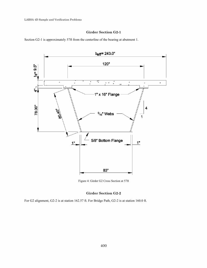
LARSA 4D Sample and Verification Problems
Girder Section G2-1
Section G2-1 is approximately 57ft from the centerline of the bearing at abutment 1.
Figure 4: Girder G2 Cross Section at 57ft
Girder Section G2-2
For G2 alignment, G2-2 is at station 162.57 ft. For Bridge Path, G2-2 is at station 160.0 ft.
400

LARSA 4D Sample and Verification Problems
Figure 5: Girder G2 Cross Section at 160ft
401

LARSA 4D Sample and Verification Problems
Deck Pouring Sequence for Constructability
Figure 6: Deck Pouring Sequence
402

LARSA 4D Sample and Verification Problems
Bearings
There are abutments and two piers, Pier 1 is at 160ft and Pier 2 is at 370ft. All supports are radial to the roadway.
There are two bearings at each girder support location. The centerline of each bearing is located 28.5” from the girdercenterline at the support. The bearings at Pier 1 are fixed against translation in both the radial and longitudinal directions- Fixed Bearings. The bearings at abutments and at Pier 2 are fixed against radial movement, but free in the longitudinaldirection – Guided Bearings.
Intermediate Cross Frames
The tub girders are braced internally at intermediate locations with K-type cross frames, where the diagonals intersectthe top strut at the top flange level.
Cross frame spacing is uniform, 16ft in end spans and 15ft in the center span.
Cross frame members have a cross sectional area of 5.0 square inches.
There is no external cross frame.
Diaphragms at the Supports
Internal diaphragms at supports, are full-depth plates with a top flange.
External diaphragms at supports, are full-depth plates with top and bottom flanges.
The web plates have a thickness of 0.5 inches.
Each flange has an area of 8.0 square inches.
Top Flange Lateral Bracing
Warren-type truss lateral bracing system is used.
The bracing is directly connected to the flanges at each internal cross frame and internal top strut.
Top flange lateral bracing members have an area of 8.0 square inches.
Figure 7: Top Flange Lateral Bracing
403

LARSA 4D Sample and Verification Problems
Dead LoadThe non-composite dead load (DC1): Permanent load before the concrete deck has hardened. The self-weight of steelgirders, cross-frames, diaphragms, lateral bracing and the concrete deck weight, haunch weight, stay-in-place metaldeck form are considered as non-composite dead loads.Steel unit weight = 490 pcf
Concrete unit weight = 150 pcf
Permanent deck form = 15 lb/ft2
The composite dead load (DC2): Superimposed dead load of parapets. The parapet weight is applied as line loadsalong the edges of deck elements.The parapet load = 495 lb/ft
The component dead load (DW): Superimposed dead load of future wearing surface.
The future wearing surface = 30 lb/ft2 (per square foot of roadway)
Live LoadHL-93 vehicular live load and a fatigue load, with the appropriate dynamic load allowance and centrifugal force effectsincluded.Highway design speed = 35 mph for centrifugal force computations
Load CombinationsStrength I load combination is used for the strength limit state
Strength I: η[1.25(DC) + 1.5(DW) + 1.75((LL+IM) + CE + BR) + 1.2(TU)]
η=1 and BR=TU=0 for this example, resulting load combination:
1.25(DC1+DC2) + 1.5(DW) + 1.75 ((LL+IM) + CE)
For constructability checks: η[1.25(D) + 1.5(C) + 1.2(WC)]
η=1 and WC=0 for this example, resulting load combination:
1.25(D) + 1.5(C)
where,
η = Load modifier
DC = Dead load: components and attachments
DW = Dead load: wearing surface and utilities
LL = Vehicular live load
IM = Vehicular dynamic load allowance
404

LARSA 4D Sample and Verification Problems
CE = Vehicular centrifugal force
WS = Wind load on structure
WL = Wind on live load
TU = Uniform temperature
BR = Vehicular braking force
D = Dead load
C = Construction loads
WC = Wind load for construction conditions from an assumed critical direction.
Modeling and Code Check in LARSA 4D - Steel Bridge Module (SBM)
Step A – Generate a new steel girder model
Choose the structure type and define the Bridge Path Alignment
405
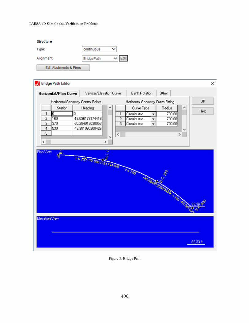
LARSA 4D Sample and Verification Problems
Figure 8: Bridge Path
406

LARSA 4D Sample and Verification Problems
Figure 9: Superelevation
The slope of the roadway (super elevation) is 5%
Bank Rotation: tan-1(0.05) = 2.86⁰
Edit Abutments and Piers
Figure 10: Abutments and Piers Spreadsheet
Station 0 ft - Abutment 1 (Guided Bearing)
Station 160 ft - Pier 1 (Fixed Bearing)
Station 370 ft - Pier 2 (Guided Bearing)
Station 530 ft – Abutment 2 (Guided Bearing)
Specify the girder type and material
Figure 11: Girder Type and Material
407

LARSA 4D Sample and Verification Problems
In the finite element analysis used in the example problem, the horizontal curvature of the girders is represented by aseries of straight elements connected at nodes. Similarly, straight girders are used in LARSA 4D.
Edit Girders
For the proper deck refinement, transverse offset values in this spreadsheet should be entered from negative to positiveor from smaller to larger. For this model, it is -11.25ft to 11.25ft.
It is also possible to enter the transverse offset values in an unordered manner, but the rule is that the smallest transverseoffset value corresponds to the smallest number of beams (first beam), the largest transverse offset value correspondsto the largest number of beams (last beam).
Figure 12: Girder Spreadsheet
The last column is the girder alignment and it is the Bridge Path along the centerline, by default.
As you can see, girder stations are entered according to corresponding girder alignment (the Bridge Path).
Web depth in this spreadsheet is the vertical web depth (for inclined webs).
Go to Tub Girder
The bottom flange T-stiffener for tub girder is a new feature. In the current version of SBM, if you have a T-stiffener,you should check if it is included in structure groups, construction stages and if its section property is properly assignedafter model generation.
408

LARSA 4D Sample and Verification Problems
Figure 13: Tub Girder Spreadsheet
409
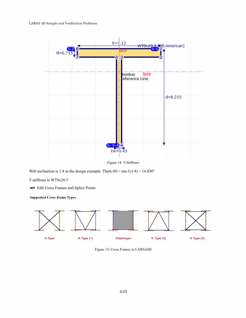
LARSA 4D Sample and Verification Problems
Figure 14: T-Stiffener
Web inclination is 1:4 in the design example. Theta (θ) = tan-1(1/4) = 14.036⁰
T-stiffener is WT8x28.5
Edit Cross Frames and Splice Points
Figure 15: Cross Frames in LARSA4D
410

LARSA 4D Sample and Verification Problems
Figure 16: Cross Frames Spreadsheet
411

LARSA 4D Sample and Verification Problems
Cross frame type in this problem is K Type (2) with no bottom chord.
Spacing of cross frames is 16’ in the end spans and 15’ in the midspan.
Go to Sections
External and internal diaphragm web plate thickness is given as 0.5in
Cross sectional area of each flange is given as 8square inches. Go to the cell in the spreadsheet that you want to definecross section of the corresponding chord (flanges). In this problem, no standard section is specified for the flanges,so we will select “(Area only)”
Similarly, cross sectional area of cross frame truss members is given as 5square inches
8 in2 = 0.05556 ft2
5 in2 = 0.03472 ft2
Figure 17: Section by Area
412

LARSA 4D Sample and Verification Problems
Figure 18: Sections Spreadsheet for Cross Frames413

LARSA 4D Sample and Verification Problems
Go to Lateral Bracings
Figure 19: Lateral Bracings in LARSA4D
Top flange lateral bracing members have an area of 8 square inches (0.05556 square feet)
414
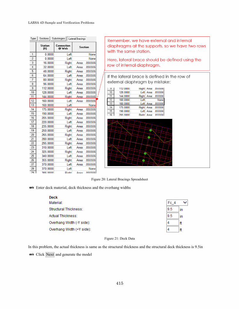
LARSA 4D Sample and Verification Problems
Figure 20: Lateral Bracings Spreadsheet
Enter deck material, deck thickness and the overhang widths
Figure 21: Deck Data
In this problem, the actual thickness is same as the structural thickness and the structural deck thickness is 9.5in
Click Next and generate the model
415

LARSA 4D Sample and Verification Problems
416

LARSA 4D Sample and Verification Problems
Figure 22: Generated Model
After model generation, you should check your model in detail.
Step B – Create Bridge Loading Data
In the example problem, the concrete deck is assumed to be placed at one time for the Strength Limit State checks.A separate analysis is performed to include deck placement sequence and results are used in constructability checks.Earlier concrete casts are composite for each subsequent cast.
Earlier concrete casts are composite for each subsequent cast.
Fill Bridge Loading Table
417

LARSA 4D Sample and Verification Problems
Figure 23: Bridge Loading Table
Go into Deck Pouring Sequence
Figure 24: Deck Pouring Data
Click Next
418

LARSA 4D Sample and Verification Problems
Figure 25: Load Cases
Perform the staged construction analysis before the code check
Comparison of the Analysis Results with the Reference Example• Unfactored shears corresponding to critical tub girder web for girder G1 is tabulated as “Table 1 Girder G1
Unfactored Shears” in the reference example. Unfactored shear forces, throughout the bridge, are taken fromLARSA 4D by “Compound Element Forces” after the staged construction analysis.
Graphical comparison of the results:
419

LARSA 4D Sample and Verification Problems
420

LARSA 4D Sample and Verification Problems
421

LARSA 4D Sample and Verification Problems
Figure 26: Girder G1 Unfactored Shears
• Unfactored major-axis bending moments for girder G1 is tabulated as “Table 3 Girder G1 Unfactored Major-Axis Bending Moments” in the reference example. Unfactored bending moments, throughout the bridge, aretaken from LARSA 4D by “Compound Element Forces” after the staged construction analysis.
Graphical comparison of the results:
422

LARSA 4D Sample and Verification Problems
423

LARSA 4D Sample and Verification Problems
424

LARSA 4D Sample and Verification Problems
Figure 27: Girder G1 Unfactored Major-Axis Bending Moments
• Unfactored shears corresponding to critical tub girder web for girder G1 is tabulated as “Table 2 Girder G2Unfactored Shears” in the reference example. Unfactored shear forces, throughout the bridge, are taken fromLARSA 4D by “Compound Element Forces” after the staged construction analysis.
Graphical comparison of the results:
425

LARSA 4D Sample and Verification Problems
426
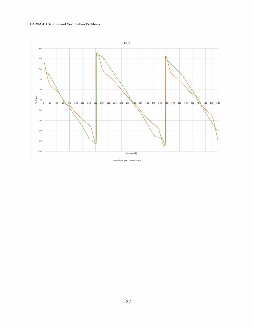
LARSA 4D Sample and Verification Problems
427

LARSA 4D Sample and Verification Problems
Figure 28: Girder G2 Unfactored Shears
• Unfactored major-axis bending moments for girder G1 is tabulated as “Table 4 Girder G2 Unfactored Major-Axis Bending Moments” in the reference example. Unfactored bending moments, throughout the bridge, aretaken from LARSA 4D by “Compound Element Forces” after the staged construction analysis.
Graphical comparison of the results:
428

LARSA 4D Sample and Verification Problems
429

LARSA 4D Sample and Verification Problems
430

LARSA 4D Sample and Verification Problems
Figure 29: Girder G2 Unfactored Major-Axis Bending Moments
In the design example, bearings are modeled with “foundation elements” in 3D Finite Element Analysis Program.These elements have six different stiffnesses as explained in the example document, however there is no informationregarding the stiffness values. Due to lack of information, bearings are modeled as supports with restraint conditionsin LARSA 4D.
The differences between analysis results of the design example and LARSA 4D are most probably due to modelingof support conditions. It is observed that, modeling supports as springs with some arbitrary stiffness values has asignificant effect on the results.
Step C – Code check per AASHTO LRFD
In this chapter, Steel Bridge Module code check inputs are illustrated for two stations which are used as positive andnegative moment design sections in the reference document.
Positive moment section, G2-1 is at 57ft in the Bridge Path Coordinate System.
Negative moment section, G2-2 is at 160ft in the Bridge Path Coordinate System.
Code check is performed in LARSA 4D Steel Bridge Module per AASHTO LRFD Bridge Design Specifications.
Detailed Verbose Report is viewed for the positive moment code check location.
Enter Code Check Locations → Locations
431

LARSA 4D Sample and Verification Problems
Figure 30: Locations
An : net cross-section area of the members
Ag : gross cross-section area of the member
rt : effective radius of gyration
Deck Reinforcing
Top layer: #6 bars at 6 inches
Bottom layer: #4 bars at 6inches
Crb and Crt are not given in the example and they are not used, cover thickness from top and bottom are taken as 1in here for 9.5in deck.
In the example, deck reinforcement is neglected in the calculation of Plastic Moment Neutral Axis for positive momentsection.
Figure 31: Deck Reinforcing
Arb : area of the bottom layer of longitudinal reinforcement within the effective concrete deck width
Art : area of the top layer of longitudinal reinforcement within the effective concrete deck width
Crb : distance from the top of the concrete deck to the centerlineof the bottom layer of longitudinal concrete deck reinforcement
Crt : distance from the top of the concrete deck to the centerlineof the top layer of longitudinal concrete deck reinforcement
fr factor : modulus of rupture factor
Transverse Stiffeners
At section G2-2, interior panel is without longitudinal stiffener and with a transverse stiffener.
Transverse stiffener: 0.5in x 5.5in
Spacing(do) = 62in
432

LARSA 4D Sample and Verification Problems
Figure 32: Transverse stiffeners
Longitudinal Stiffeners
T-stiffener data is to be entered under Tub Data
Tub Data
T-stiffener is WT8x28.5
Figure 33: Bottom Flange Stiffener Definition in LARSA4D
Figure 34: T-Stiffener
D : the depth of web plate measured along the slope (for inclined webs)
433

LARSA 4D Sample and Verification Problems
w : larger of the width of a box flange between longitudinal flange stiffenersor the distance from a web to the nearest longitudinal flange stiffener
Fatigue
Fatigue I load combination is used in combination with design checks for infinite fatigue life.
Figure 35: Fatigue
Result cases are assigned to load classes and load factors are modified to have Strength-I, Service-II and1.25*(dead load) +1.5*(construction load) for constructability.
Construction Girder Details
The top flange is continuously braced by the concrete deck for strength limit state.
The top flange is discretely braced for constructability (deck is not hardened).
Even if you leave these inputs as default, we are setting them according to your model when performing the code check.
Click Next and perform the code check.
Code Check Summary• Girder Properties
Figure 36: Summary Report Girder Properties
• Section Properties
434

LARSA 4D Sample and Verification Problems
Figure 37: Summary Report Section Properties
Comparison with the design example for Section G2-2
NoncompositeExample LARSA4D
Composite,3nExample LARSA4D
Composite,nExample LARSA4D
A 338.27 332.057 A 440.07 434.21 A 643.67 638.513
I 439269 427386 I 631237 637005 I 833731 855766
cgtop 43.68 44.64 cgtop 32.25 32.47 cgtop 20.23 19.82
cgbot 38.82 37.87 cgbot 50.25 50.03 cgbot 62.27 62.68
Stop 10056 9575 Stop 19575 19618 Stop 41217 43180
Sbot 11316 11287 Sbot 12561 12733 Sbot 13388 13653
In design example, bottom flange stiffener and the longitudinal component oftop flange lateral bracing area is included in section property calculations.
In LARSA 4D Code Check, section properties are calculated including the bottomflange stiffener if present. The top flange lateral bracing is not included and the
reason for the difference between design example and the LARSA 4D is that.
• Force Summary
435
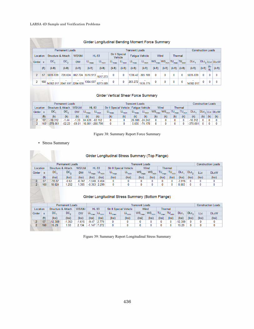
LARSA 4D Sample and Verification Problems
Figure 38: Summary Report Force Summary
• Stress Summary
Figure 39: Summary Report Longitudinal Stress Summary
436

LARSA 4D Sample and Verification Problems
Figure 40: Summary Report Lateral Stress Summary
• Flexural Resistance
Figure 41: Summary Report Flexural Resistance
• Performance ratios as a result of the code check
Figure 42: Performance Ratios
437

LARSA 4D Sample and Verification Problems
The Summary and the Verbose Reports
In this chapter, rather than the numerical comparisons, the code check procedures of the Steel Bridge Module will bereviewed which are verified by the design procedures of the example problem.
If you click on the station that you performed the code check from the menu, you will see pass and fail results in theSummary Report:
(You have an option at that page to see the verbose report)
Figure 43: Summary Report
The Code Check Procedures in the Verbose Report
Reference Document: AASHTO LRFD (7th Edition, 2014)
• Section Proportioning
Figure 44: Section Proportioning
438

LARSA 4D Sample and Verification Problems
1) AASHTO Article 2.5.2.6.3 Optional Criteria for Span-to-Depth Ratios
“For curved girder systems, the span-to-depth ratio, L/D, of each steel girder should not exceed 25 when the specifiedminimum yield strength of the girder in regions of positive flexure is 50ksi or less.”
2) AASHTO Article 6.11.2.1 Web Proportions
For the case of inclined webs, the distance along the web shall be used for checking all design requirements
D/tw ≤ 150 (webs with longitudinal stiffener)[6.11.2.1.2-1]
D/tw ≤ 300 (webs without longitudinal stiffener)[6.11.2.1.2-2]
da: the depth of web plate measured along the slope (report)
3) AASHTO Article 6.11.2.2 Flange Proportions
bf/2tf ≤ 12 [6.11.2.2.2-1]
bf ≥ D/6 [6.11.2.2.2-2]
bf/2tf ≥ 1.tw1 [6.11.2.2.2-3]
4) AASHTO Article 6.11.1.1 Stress Determinations
If the flange width exceeds one-fifth of the effective span, only a width equal to one-fifth of the effective span shallbe considered effective in resisting flexure.
In this example, the flange width does not exceed one-fifth of the effective span where the effective length of span is128ft, so, bf_bot = 83in is used for stress calculations.
5) AASHTO Article 6.11.2.1.1 General
The inclination of the web plates to a plane normal to the bottom flange should not exceed 1 to 4
• Strength Limit State - Flexural Resistance (Positive Moment Region)
Figure 45: Flexural Resistance
6) AASHTO Article 6.11.6.2.2 Sections in Positive Flexure
Sections in horizontally curved steel girder bridges shall be considered as noncompact sections and shall satisfy therequirements of Article 6.11.7.2
Compact and noncompact sections shall satisfy the ductility requirement specified in Article 6.10.7.3
439
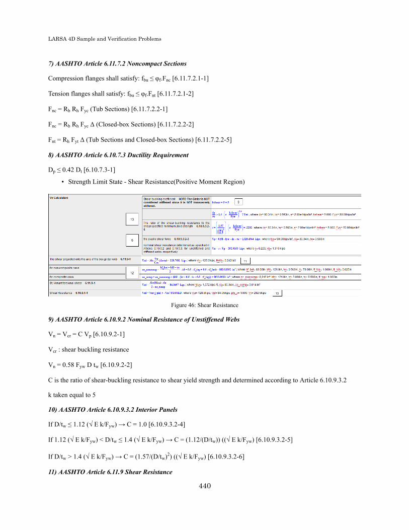
LARSA 4D Sample and Verification Problems
7) AASHTO Article 6.11.7.2 Noncompact Sections
Compression flanges shall satisfy: fbu ≤ φf.Fnc [6.11.7.2.1-1]
Tension flanges shall satisfy: fbu ≤ φf.Fnt [6.11.7.2.1-2]
Fnc = Rb Rh Fyc (Tub Sections) [6.11.7.2.2-1]
Fnc = Rb Rh Fyc Δ (Closed-box Sections) [6.11.7.2.2-2]
Fnt = Rh Fyt Δ (Tub Sections and Closed-box Sections) [6.11.7.2.2-5]
8) AASHTO Article 6.10.7.3 Ductility Requirement
Dp ≤ 0.42 Dt [6.10.7.3-1]
• Strength Limit State - Shear Resistance(Positive Moment Region)
Figure 46: Shear Resistance
9) AASHTO Article 6.10.9.2 Nominal Resistance of Unstiffened Webs
Vn = Vcr = C Vp [6.10.9.2-1]
Vcr : shear buckling resistance
Vn = 0.58 Fyw D tw [6.10.9.2-2]
C is the ratio of shear-buckling resistance to shear yield strength and determined according to Article 6.10.9.3.2
k taken equal to 5
10) AASHTO Article 6.10.9.3.2 Interior Panels
If D/tw ≤ 1.12 (√ E k/Fyw) → C = 1.0 [6.10.9.3.2-4]
If 1.12 (√ E k/Fyw) < D/tw ≤ 1.4 (√ E k/Fyw) → C = (1.12/(D/tw)) ((√ E k/Fyw) [6.10.9.3.2-5]
If D/tw > 1.4 (√ E k/Fyw) → C = (1.57/(D/tw)2) ((√ E k/Fyw) [6.10.9.3.2-6]
11) AASHTO Article 6.11.9 Shear Resistance
440
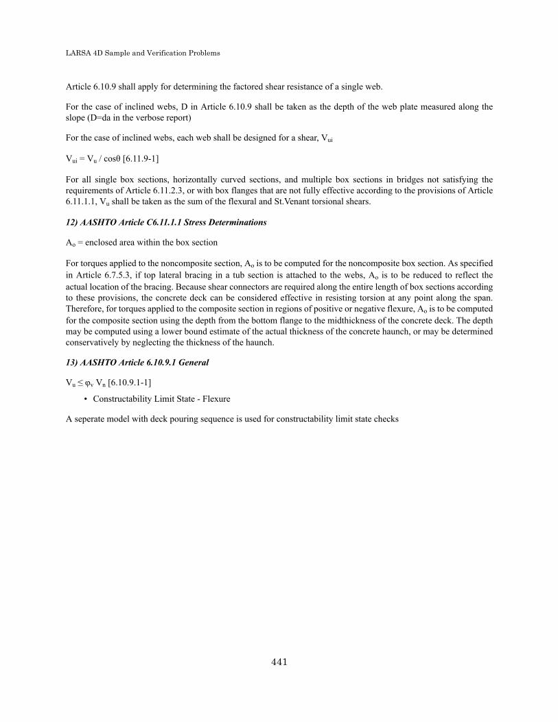
LARSA 4D Sample and Verification Problems
Article 6.10.9 shall apply for determining the factored shear resistance of a single web.
For the case of inclined webs, D in Article 6.10.9 shall be taken as the depth of the web plate measured along theslope (D=da in the verbose report)
For the case of inclined webs, each web shall be designed for a shear, Vui
Vui = Vu / cosθ [6.11.9-1]
For all single box sections, horizontally curved sections, and multiple box sections in bridges not satisfying therequirements of Article 6.11.2.3, or with box flanges that are not fully effective according to the provisions of Article6.11.1.1, Vu shall be taken as the sum of the flexural and St.Venant torsional shears.
12) AASHTO Article C6.11.1.1 Stress Determinations
Ao = enclosed area within the box section
For torques applied to the noncomposite section, Ao is to be computed for the noncomposite box section. As specifiedin Article 6.7.5.3, if top lateral bracing in a tub section is attached to the webs, Ao is to be reduced to reflect theactual location of the bracing. Because shear connectors are required along the entire length of box sections accordingto these provisions, the concrete deck can be considered effective in resisting torsion at any point along the span.Therefore, for torques applied to the composite section in regions of positive or negative flexure, Ao is to be computedfor the composite section using the depth from the bottom flange to the midthickness of the concrete deck. The depthmay be computed using a lower bound estimate of the actual thickness of the concrete haunch, or may be determinedconservatively by neglecting the thickness of the haunch.
13) AASHTO Article 6.10.9.1 General
Vu ≤ φv Vn [6.10.9.1-1]
• Constructability Limit State - Flexure
A seperate model with deck pouring sequence is used for constructability limit state checks
441

LARSA 4D Sample and Verification Problems
Figure 47: Constructability - Flexure
AASHTO Article 6.11.3.1 General: The provisions of Article 6.10.3 shall apply.
14) AASHTO Article 6.11.3.2 Flexure
For critical stages of construction, the provisions of 6.10.3.2.1 through 6.10.3.2.3 shall be applied only to the topflanges of tub sections.
Continuously braced box flanges in tension or compression shall satisfy :
fbu ≤ φf Rh fyf Δ [6.11.3.2-3]
For loads applied to a composite box flange before the concrete has hardened or is made composite, the flange shallbe designed as a noncomposite box flange. The maximum vertical deflection of the noncomposite box flange due tothe unfactored permanent loads, including the self-weight of the flange plus the unfactored construction loads, shallnot exceed 1/360 times the transverse span between webs. (Not checked in the design example)
The through-thickness bending stress in the noncomposite box flange due to the factored permanent loads and factoredconstruction loads shall not exceed 20.0 ksi.
15) AASHTO Article 6.10.3.2.1 Discretely Braced Flanges in Compression
fbu + fl ≤ φf Rh Fyc [6.10.3.2.1-1]
fbu + 1/3 fl ≤ φf Fnc [6.10.3.2.1-2]
fbu ≤ φf Fcrw [6.10.3.2.1-3]
Fnc shall be determined as specified in Article 6.10.8.2
442

LARSA 4D Sample and Verification Problems
In computing Fnc for constructability, the web load-shedding factor, Rb, shall be taken as 1.0
16) AASHTO 6.10.8.2.1 General
Fnc, shall be taken as the smaller of the local buckling resistance (fnc_flb in the verbose report) determined as specifiedin Article 6.10.8.2.2, and the lateral torsional buckling resistance (fnc_ltb in the verbose report) determined as specifiedin Article 6.10.8.2.3.
17) AASHTO Article 6.10.1.6 Flange Stresses and Member Bending Moments
All discretely braced flanges shall satisfy :
fl ≤ 0.6 Fyf [6.10.1.6-1]
• Constructability Limit State - Shear
Similar to strength limit state except that St. Venant torsional shear is not considered.
Figure 48: Constructability - Shear
AASHTO Article 6.11.3.3 Shear: the provisions of Article 6.10.3.3 and 6.11.9 apply
AASHTO Article 6.10.3.3 Shear: Vu ≤ φv Vcr [6.10.3.3-1] where Vcr is the shear buckling resistance determined fromEq. 6.10.9.3.3-1
AASHTO 6.10.9.3.3 End Panels: Vn = Vcr = C Vp [6.10.9.3.3-1] in which Vp = 0.58 Fyw D tw [6.10.9.3.3-2]
• Service Limit State
Figure 49: Serviceability
443

LARSA 4D Sample and Verification Problems
AASHTO Article 6.11.4 Service Limit State: The fℓ term in Eq. 6.10.4.2.2-2 shall be taken equal to zero. Eq.6.10.4.2.2-3 shall not apply. Except for sections in positive flexure in which the web satisfies the requirement of Article6.11.2.1.2, all sections shall satisfy Eq. 6.10.4.2.2-4
18) AASHTO Article 6.10.4.2.2 Flexure
For the top steel flange of composite sections :
ff ≤ 0.95 Rh Fyf [6.10.4.2.2-1]
For the bottom steel flange of composite sections:
ff + fℓ/2 ≤ 0.95 Rh Fyf [6.10.4.2.2-2]
• Fatigue Limit State
Figure 50: Fatigue Limit State
AASHTO Article 6.11.5 Fatigue and Fracture Limit State: The provisions of Article 6.10.5 apply.
AASHTO Article 6.10.5.1 Fatigue: Details shall be investigated for fatigue as specified in Article 6.6.1. The applicableFatigue load combination specified in Table 3.4.1-1 and fatigue live load specified in Article 3.6.1.4 shall apply. Forhorizontally curved I-girder bridges, the fatigue stress range due to major-axis bending plus lateral bending shall beinvestigated.
19) AASHTO Article 6.6.1.2.5 Fatigue Resistance
The nominal fatigue resistance for Fatigue I load combination and infinite life :
(ΔF)n = (ΔF)TH [6.6.1.2.5-1]
Constant amplitude fatigue threshold for Detail Category C':
(ΔF)TH = 12 [Table 6.6.1.2.5-3]
20) AASHTO Article 6.6.1.2.2 Design Criteria
For load-induced fatigue considerations, each detail shall satisfy :
γ (Δf) ≤ (ΔF)n [6.6.1.2.2-1]
γ: load factor specified in Table 3.4.1-1 for the fatigue load combination (Ftgamma in the verbose report)
(Δf): force effect, live load stress range due to the passage of the fatigue load as specified in Article 3.6.1.4 (FSRBotin the verbose report)
• Strength Limit State - Flexural Resistance (Negative Moment Region)
444

LARSA 4D Sample and Verification Problems
Figure 51: Flexural Resistance
AASHTO Article 6.11.6.2.3 Sections in Negative Flexure: The provisions of Article 6.11.8 shall apply.
AASHTO Article 6.11.8.2.1 General: The nominal flexural resistance of box flanges in compression without flangelongitudinal stiffeners shall be determined as specified in Article 6.11.8.2.2. The nominal flexural resistance of boxflanges in compression with flange longitudinal stiffeners shall be determined as specified in Article 6.11.8.2.3.
21) AASHTO Article 6.11.8.2.3 Longitudinally Stiffened Flanges: The nominal flexural resistance of the compressionflange shall be taken as equal to the nominal flexural resistance for the compression flange without longitudinalstiffeners, determined as specified in Article 6.11.8.2.2, with the following substitutions
bfc = w
k = (8 Is / w t3fc)1/3 for n = 1 [6.11.8.2.3-1]
445

LARSA 4D Sample and Verification Problems
k = (0.894 Is / w t3fc)1/3 for n = 2 [6.11.8.2.3-2]
1.0 ≤ k ≤ 4.0
The plate buckling coefficient for shear stress ks shall be taken as:
ks = ( 5.34 + 2.84 (Is / w t3fc)1/3 ) / (n + 1)2 ≤ 5.34 [6.11.8.2.3-3]
22) AASHTO Article 6.11.8.2.2 Unstiffened Flanges
The nominal flexural resistance of the compression flange, Fnc shall be taken as:
Fnc = Fcb √ 1 - (fv / φv Fcv)2 [6.11.8.2.2-1]
If λf ≤ λp, Fcb = Rb Rh Fyc Δ [6.11.8.2.2-2]
If λp < λf ≤ λr, Fcb = Rb Rh Fyc (Δ - (Δ - (Δ - 0.3)/Rh) ((λf - λp)/(λr - λp))) [6.11.8.2.2-3]
If λf > λr, Fcb = 0.9 E Rb k / λ2f [6.11.8.2.2-4]
If λf ≤ 1.12 (√ E ks/Fyc), Fcv = 0.58 Fyc [6.11.8.2.2-5]
If 1.12 (√ E ks/Fyc) < λf ≤ 1.4 (√ E ks/Fyc), Fcv = (0.65 √ Fyc E ks) / λf [6.11.8.2.2-6]
If λf > 1.4 (√ E ks/Fyc), Fcv = 0.9 E ks / λ2f [6.11.8.2.2-7]
λf = bfc / tfc [6.11.8.2.2-8]
λp = 0.57 √ E k/Fyc Δ [6.11.8.2.2-9]
λr = 0.95 √ E k/Fyr [6.11.8.2.2-10]
23) AASHTO Article 6.11.8.1.1 Box Flanges in Compression
fbu ≤ φf Fnc [6.11.8.1.1-1]
24) AASHTO Article 6.11.8.3 Tension-Flange Flexural Resistance
The nominal flexural resistance of the tension flanges of tub sections shall be taken as:
Fnt = Rh Fyt [6.11.8.3-1]
25) AASHTO Article 6.11.8.1.2 Continuously Braced Flanges in Tension
fbu ≤ φf Fnt [6.11.8.1.2-1]
• Strength Limit State - Shear Resistance (Negative Moment Region)
446

LARSA 4D Sample and Verification Problems
Figure 52: Shear Resistance
26) AASHTO Article 6.11.9 Shear Resistance
Article 6.10.9 shall apply for determining the factored shear resistance of a single web.
For the case of inclined webs, D in Article 6.10.9 shall be taken as the depth of the web plate measured along theslope (D=da in the verbose report)
For the case of inclined webs, each web shall be designed for a shear, Vui
Vui = Vu / cosθ [6.11.9-1]
For all single box sections, horizontally curved sections, and multiple box sections in bridges not satisfying therequirements of Article 6.11.2.3, or with box flanges that are not fully effective according to the provisions of Article6.11.1.1, Vu shall be taken as the sum of the flexural and St.Venant torsional shears.
27) AASHTO Article 6.10.9.1 General
At the strength limit state, straight and curved web panels shall satisfy:
Vu ≤ φv Vn [6.10.9.1-1]
Transverse intermediate stiffeners shall be designed as specified in Article 6.10.11.1.
Interior web panels of nonhybrid and hybrid I-shaped members:
-without a longitudinal stiffener and with a transverse stiffener spacing not exceeding 3D
-with one or more longitudinal stiffeners and with a transverse stiffener spacing not exceeding 1.5D
shall be considered stiffened, and the provisions of Article 6.10.9.3 shall apply.
447

LARSA 4D Sample and Verification Problems
For box flanges, bfc or bft, as applicable, shall be taken as one-half of the effective flange width between webs inchecking Eq. 6.10.9.3.2-1, where the effective flange width shall be taken as specified in Article 6.11.1.1, but not toexceed 18tf where tf is the thickness of the box flange.
28) AASHTO Article 6.10.9.3.2 Interior Panels
The nominal shear resistance of an interior web panel complying with the provisions of Article 6.10.9.1, and with thesection along the entire panel proportioned such that:
2 D tw / (bfc tfc + bft tft) ≤ 2.5 [6.10.9.3.2-1]
shall be taken as:
Vn = Vp (C + 0.87(1 - C) / (√ 1 + (do / D)2)) [6.10.9.3.2-2]
Vp = 0.58 Fyw D tw [6.10.9.3.2-3]
If D/tw ≤ 1.12 (√ E k/Fyw) → C = 1.0 [6.10.9.3.2-4]
If 1.12 (√ E k/Fyw) < D/tw ≤ 1.4 (√ E k/Fyw) → C = (1.12/(D/tw)) ((√ E k/Fyw) [6.10.9.3.2-5]
If D/tw > 1.4 (√ E k/Fyw) → C = (1.57/(D/tw)2) ((√ E k/Fyw) [6.10.9.3.2-6]
k = 5 + 5 / (do / D)2 [6.10.9.3.2-7]
• Constructability Limit State - Flexure (Negative Moment Region)
448

LARSA 4D Sample and Verification Problems
Figure 53: Constructability-Flexure
29) AASHTO Article 6.10.3.2.2 Discretely Braced Flanges in Tension
fbu + fl ≤ φf Rh Fyt [6.10.3.2.2-1]
30) AASHTO Article 6.11.3.2 Discretely Braced Flanges in Tension
fbu ≤ φf Fnc [6.11.3.2-1]
fbu ≤ φf Fcrw [6.11.3.2-2]
For sections with compact or noncompact webs, Eq. 6.11.3.2-2 shall not be checked.
• Constructability Limit State - Shear (Negative Moment Region)
Similar to strength limit state except that St. Venant torsional shear is not considered.
449

LARSA 4D Sample and Verification Problems
Figure 54: Constructability-Shear
Note: According to AASHTO Article 6.11.7.2.1 the maximum longitudinal compressive stress in the concrete deck atthe strength limit state is limited. This check is to be added inside the Steel Bridge Module Code Check Proceduresin the next release.
References• U.S. Department of Transportation Federal Highway Administration. (2015, December). Steel Bridge Design
Handbook Design Example 5. Retrieved from www.fhwa.dot.gov: https://www.fhwa.dot.gov/bridge/steel/pubs/hif16002/designexample06.pdf
• AASHTO LRFD Bridge Design Specifications ( 7th Edition, 2014 )
450

LARSA 4D Sample and Verification Problems
Samples for CompositeConstruction
These samples provide an overview of the composite section construction.
C01: Single Span with Roller under Vertical Load 453Cross-Section Definition 453Model 455Cross-Sectional Properties 456Self-Weight Loading 457
C02: Staged Construction Analysis 461Composite Sequence States 461Self-Weight Loading 462Standard Staged Construction Analysis 463
C03: Time-Dependent Material Properties 469Cross-Section Definition 469Model 469Cross-Sectional Properties 470Self-Weight Loading 471Time Effect on Elastic Modulus 472Shrinkage 474Creep 477References 477
C04: Thermal Loads 479Cross-Section Definition 479Model 481Analysis of Thermal Loads 481Uniform Thermal Load 482Linear Gradient Thermal Load 483Nonlinear Gradient Thermal Load 485
451

LARSA 4D Sample and Verification Problems
452
LARSA 4D Sample and Verification Problems
C01: Single Span with Roller underVertical Load
A simply supported beam is used to verify several aspects of the analysis of composite sections in a static analysis.The length of the span is 300 ft, and it has a composite cross-section comprised of a steel I-shape girder and a concreterectangular-shape deck. Section properties of the composite cross-section and behavior of the beam (displacement,member force, and member stress) under self-weight loading is verified.
Example Project: The example described here can be found in the Composite Construction folder of your LARSA4D Samples directory (generally My Documents\LARSA Projects\Samples) in the file C01.
Cross-Section DefinitionThe cross-section used in this problem is composed of a steel I-shape and a concrete slab on top. The dimensions are:
• I-Shape: 5 ft deep; 2 ft wide; 0.2 ft flange and web thickness
• Rectangle Shape: 0.8 ft deep; 4 ft wide
This is created in LARSA Section Composer. Stress Recovery Points must be set on the section at this point todetermine where LARSA 4D will report stresses later. This example includes six Stress Recovery Points: 1-4 clockwisearound the I-shape, and 5 and 6 at the upper-right and upper-left of the concrete slab, respectively.
453

LARSA 4D Sample and Verification Problems
Figure 1: Cross-Section
Note that the shapes are placed such that the reference axes (the joint-to-joint line) are at the centroid of the deck slab.
Two additional steps are taken for composite sections.
The material of each shape is set in LARSA Section Composer. For a composite section with multiple materials, it isnot possible to set the member’s materials in LARSA 4D. The materials of all shapes must be set in Section Composer.The materials A36 (for the I-Shape) and Fc_4 (for the Rectangle Shape) are set in Section → Composite Materials .A Base Material can be chosen at this point which is used in the display of the cross-section properties (here and inLARSA 4D) but ultimately does not affect the analysis.
454

LARSA 4D Sample and Verification Problems
ModelThe girder and deck system is modeled as a single composite beam as defined in the previous section. The beam issupported by a pin on one end and a roller at the other, with the supports level with the centroid of the deck. Thelength of the span is 300 ft. The span is divided into 10 segments. This is a 2D problem: TY, RX, and RZ are fixedas universal restraints.
The composite model is not assigned a material in LARSA 4D as the materials of the shapes have been set in LARSASection Composer. Although the model has no member end offsets, because the reference axes of the cross-section arepositioned in Section Composer to align with the centroid of the deck shape, the I girder shape is located below thejoints, i.e., shifted down, automatically. The girder is along the x-axis with the z-axis parallel to the web. The membershave an orientation angle of 90 degrees.
A verification of the results of a composite section model is made by comparing the results to hand calculations andto roughly equivalent reference models using non-composite elements.
Non-composite reference models A and B are each made using a line of member elements for the concrete part anda separate line of member elements for the steel part. The two lines are divided into ten segments and are rigidlyconnected at the eleven points along those lines. Two options for rigid connections exist in LARSA 4D. Referencemodel A uses member elements with high stiffness between pairs of joints to connect the two lines of members atthe 11 intermediate joints. There are 22 joints in this model and 30 member elements. The joints are positioned at thecentroids of the members.
Reference model B uses member end offsets to connect the two lines of members to the same joints while stillpositioning the members at their appropriate locations. The deck elements go from joint 1 to joint 2, from joint 2 tojoint 3, and so on. The girder elements have identical connectivity (joint 1 to joint 2, joint 2 to joint 3, etc.), exceptmember end offsets are used to shift the I-shaped elements down by 2.9 ft, the distance from the centroid of the slabto the centroid of the girder. (In other words, the I-Offset Z and the J-Offset Z are set to -2.9 for the girder elements.)There are 11 joints and 20 member elements in this model.
Reference model C is made entirely using plate elements, one for the web, two for the flanges (one top, one bottom),and one for the slab. Plate end offsets are used so that the plate connective in each cross-section is to the same joint.This is highly unusual but appropriate for a comparison with the composite model. In other words, the connectivity ofthe first plate for the slab is joint 1-joint 1-joint 2-joint 2. Plate end offsets set the Y offset of the plate to -2 ft, 2 ft, 2ft, -2 ft. In other words, the I-coordinate of the plate is joint 1 minus 2 ft in the y direction. The J-coordinate is joint 1plus 2 ft in the y direction. And so on. This will mimic the behavior of member element cross sections in which planesections remain plane. The Thick (PQ2) with Drilling shell formulation is used.
The C01 project file includes the composite model and the reference models together. The composite model is on theleft, followed by the reference models A, B, and C from left to right.
Figure 3: Models
455

LARSA 4D Sample and Verification Problems
Figure 4: Models with Rendering
Cross-Sectional PropertiesCross-sectional properties of the composite section are computed for the section as a whole as well as for eachconstruction sequence state.
The centroid of the cross-section is computed by Section Composer as 2.356 ft below the reference axes (at the centroidof the concrete part). This is readily verified by hand as the sum of the centroid locations of the shapes (relative to thereference axes) times their modulus of elasticity and area divided by the total E×A.
Section Centroid Computation and Basic Shape Properties
CentroidLocation (c)
(ft)
E(kip/ft2)
A(ft2)
c×E×A(kip-ft)
c×E×A/ΣEA(ft)
Concrete 0 519,120 3.20 0 0
Steel -2.9 4,176,000 1.72 -20,829,888 −2.355
Total E×A: 8,843,904
The properties for the section as a whole as given by Section Composer, with concrete as the reference material, aregiven in the table below. Units are feet. Hand calculations verify A, Iyy, and Izz easily. The total cross-sectional area isthe sum of the factored properties of the two shapes. Each shape’s properties are factored by the ratio of its modulus ofelasticity to that of the reference material. The moment of inertia in y is computed in this same way. In z, the moment ofinertia is additionally transformed by adding the shape’s area times the square of the distance from the shape’s centroidto the section centroid, and is then factored.
Section Properties Computation
Concrete Part Steel Part Composite
Base Transformed Base Transformed Factored
A (ft2) 3.20 --- 1.72 --- 13.8 17.0
Iyy (ft4) 4.27 --- 0.270 --- 2.17 6.44
Izz (ft4) 0.171 17.9 6.23 6.74 54.2 72.2
456

LARSA 4D Sample and Verification Problems
Concrete Part Steel Part Composite
J (ft4) 0.588 --- 0.0229 --- --- 1.49
LARSA 4D’s computations match the hand calculation to within rounding error. There is no hand verification for thetorsion constant J at this time. The value for J computed by the Section Composer is listed above for reference.
Self-Weight LoadingThe results of the test model and the reference models in LARSA 4D are compared to hand calculations.
The total magnitude of self-weight on the structure is the sum of the self-weight for each piece.
Hand Calculation of Total Self-Weight Load
Area (ft2) Length (ft) Density (kip/ft3) Total Weight (kip)
Steel 1.72 300 0.49 253
Concrete 3.20 300 0.15 144
397
We can compare this with the sum of the z-reactions reported in the three reference models and the composite testmodel. The reactions sum to the correct total within three significant digits.
The next verification is for displacements. The maximum deflection at mid-span is given by
δ = 5/384×(W×L3)/(E×I)
W = 397 kip, as given in the previous table. L = 300 ft. E is the modulus of elasticity of the reference material (givenabove). I is the moment of inertia about Z for the composite section (based on the choice of reference material). Asimilar hand calculation is given for deflection at 20% of the length of the span.
Deflections
@ 20% of Span @ Mid-Span (ft)
Deflection (ft) Error (%) Deflection (ft) Error (%)
Hand Calc. 2.21 3.72
Composite 2.21 <1% 3.73 <1%
Reference A 2.23 1% 3.75 1%
Reference B 2.23 1% 3.75 1%
Reference C 2.06 -6% 3.47 -8%
The axial force acting on each of the two shapes is computed. Because of the end restraints, there is no pure axial force atthe centroid of the composite beam. However, bending of the beam causes strain at other locations, and consequently the
457

LARSA 4D Sample and Verification Problems
two shapes that make up the composite beam are carrying axial force, with the I-Shape in tension and the rectangular-shape in compression. The strain distribution on the shapes is computed byε = cM/EIzz
where M is the moment acting at the centroid of the beam, c is the distance between the centroid and a particlarfiber, and EIzz is the property of the composite section. Then, multiplying the strain with the elastic modulus of thecorresponding shape provides the stress at the chosen fiber. Integrating the stress distribution over the area of eachshape gives the total axial force acting on that shape due to bending.
The non-composite and composite models differ significantly in the reported axial force in the members. The referencemodels show step-wise variation. The force within each member element is constant, and there are large breaks at thediscrete points of rigid connections. On the other hand, the composite model shows a smooth axial force curve acrossthe entire length of the model. The force at the end of each element is equal to the force at the start of the next.
However, we can see that the computations agree at a larger scale. The average of the start and end force of eachmember in the composite model is close to the corresponding force in either of the two member reference models.But because the axial force curve in the composite model is parabolic and not linear, the correct comparison is not theaverage of the end forces but the average value of the parabolic force curve (i.e., the area under the curve divided bythe member length), F'. The start and end forces, the F' force, and the axial forces in the two member-based referencemodels, are shown below at two locations on the models. For Reference Model C, Compound Element Forces are usedto obtain the forces at the composite element centroid of the plate elements that make up the I-Section shape.
Axial Force in Steel I-Shape. Units are kip
Location Member 1 Member 5
Start End F' Start End F'
Hand Calc. 0 560 290 1,492 1,554 1,533
Composite 0 560 1,492 1,554
Reference A 290 290 1,533 1,533
Reference B 290 290 1,533 1,533
Reference C 280 280 1,497 1,497
The next comparison is member stresses. Care must be taken to compare stresses at equivalent stress recovery points,as they may not be numbered in the same manner between the three member-based models.
Stresses at the start of the model and at mid-span are given below. Note that Stress Recovery Points 1-4 are in the steelI-shape while points 5-6 are in the concrete slab. Stresses in the deck (point 5) in Reference Model C are reported fromthe Plate Stresses at Joints, maximum Principal Stress.
There is no strain at the compound centroid in a model with loading such as this. Stresses are due entirely to the bendingstress. Further, at the pin supports there is no bending stress.
The stress at mid-span can be computed by first computing the rotational strain, the slope of the strain curve along themember’s y-axis. The rotational strain of the compound section is assumed to be the same as the rotational strain ofeach shape in a composite section in order to enforce the requirement of plane sectionsremaining plane (assuming the shapes were constructed at the same time). The rotational strain is given byM/EIzz = 3.97e-4
458

LARSA 4D Sample and Verification Problems
whereM = WL/8 = 14,888 kip-ft
and E and Izz are the composite section properties as given in the table above. This can be converted into a stress foreach shape by multiplying it by the modulus of elasticity of the shape and the distance from the stress recovery pointto the section centroid (point 3: 3.044 ft; point 5: 2.756 ft).
Stresses. Units are kip/ft2
@ Start @ Mid-Span
Stress Point 3 5 3 5
Hand Calc. 0 0 5,050 568
Composite 0 0 5,050 568
Reference A 152 185 5,077 479
Reference B 152 185 5,077 479
Reference C 939 97 1,497 1,497
The differences between the non-composite models on the one hand and the hand calc and composite model on theother are significant here. The stresses follow a similar pattern as the shape axial forces: the reference models exhibitstep-wise changes at the joints, while the composite model has a smooth stress curve over the length of the span.
459

LARSA 4D Sample and Verification Problems
460

LARSA 4D Sample and Verification Problems
C02: Staged Construction Analysis
A beam with fully fixed supports on both ends is used to verify several aspects of the analysis of composite sections instatic and standard Staged Construction Analysis. The length of the span is 300 ft, and it has a composite cross-sectioncomprised of a steel I-shape girder and a concrete rectangular-shape deck.
Example Project: The example described here can be found in the Composite Construction folder of your LARSA4D Samples directory (generally My Documents\LARSA Projects\Samples) in the file C02.
The model in this verification sample is identical to that in problem C01: Single Span with Roller under Vertical Load(page 453) except that the span is fully supported on both ends and composite sequence states are added to the cross-section definition in LARSA Section Composer.
Composite Sequence StatesThe shapes of the cross-section will be added at different times during construction in the Staged Construction Analysisverification. Construction Sequence States must be defined. A Construction Sequence State is a configuration of thecross-section that will be needed later. In each configuration, each shape is either:
• Active
• Active with Stiffness Only (self-weight is deferred)
• Weight Only (no stiffness)
• Inactive
No Construction Sequence State is needed specifically for the case when all shapes are active. In this example, wherethe girder is erected first, a Construction Sequence State is needed that includes the I girder as active and the slab asinactive. Since the deck pour is modeled in a weight-only then stiffness manner, two Construction Sequence Statesare needed:
State A
• I Girder: Active
• Slab: Inactive
State B
• I Girder: Active
• Slab: Weight Only
State C
• I Girder: Active
• Slab: Active
The state with both shapes Active is implicitly defined. Consequently, it is not necessary to define State C explicitly.
Construction Sequence States can be defined in any order (i.e. what is State A versus what is State B doesn’t matter).
To define a Construction Sequence State, change to the Const. Seq. tab of the Shapes Explorer:
461

LARSA 4D Sample and Verification Problems
Figure2: Construction Sequence
To add a state, click on Add State . Then for each shape active in the state, select the shape in the drawing canvas, andthen click Add Shape in the construction sequence panel.
To toggle a shape through the different shape modes like weight-only, click the name of the shape in the list and thenclick the WS button at the top of the list.
In the two Construction Sequence States, the concrete slab is omitted from the cross-section analysis. As a result, thetotal properties of the cross-section are the same as that of the steel I-shape alone. The centroid of the cross section inthese states is located at the centroid of the I-shape (2.9 ft below the reference axis).
Self-Weight LoadingThe first verification is for displacements. The maximum deflection at mid-span is given by
δ = 1/384×(W×L3)/(E×I)
where W = 397 kips, L = 300 ft., E is the modulus of elasticity of the reference material, and I is the moment of inertiaabout Z for the composite section (based on the choice of reference material), all as in C01 (page 453).
The results of the test model and the reference models in LARSA 4D are compared to hand calculations.
Deflections
@ Mid-Span (ft)
Deflection (ft) Error (%)
Hand Calc. 0.745
Composite 0.749 1%
Reference A 0.767 3%
462

LARSA 4D Sample and Verification Problems
@ Mid-Span (ft)
Reference B 0.767 3%
Reference C 0.682 -8%
The next comparison is member stresses. Stresses at the start of the model and at mid-span are given below. Note thatStress Recovery Points 1-4 are in the steel I-shape while points 5-6 are in the concrete slab. Stresses in the deck (point5) in Reference Model B are reported from the Plate Stresses at Joints, Principal Stress.
There is no strain at the compound centroid in a model such as this. Stresses are due entirely to the bending stress.The stress at mid-span can be computed by first computing the bending strain. The bending strain of the compoundsection is assumed to be the same as the bending strain of each shape in a composite section (assuming the shapeswere constructed at the same time). The bending strain is given byε = cM/EIzz
where at the startM = WL/12 = 9,925 kip-ft
yielding a bending strain of 2.65e-4, and at mid spanM = WL/24 = 4,963 kip-ft
giving a bending strain of 1.32e-4. E and Izz are the composite section properties as given in the table at the start ofC01 (page 453). This can be converted into a stress for each shape by multiplying it by the modulus of elasticity of theshape and the offset of the stress recovery point from the section centroid (point 3: 3.044 ft; point 5: 2.756 ft).
Stresses. Units are kip/ft2
@ Start @ Mid-Span
Stress Point 3 5 3 5
Hand Calc. 3,370 379 1,680 189
Composite 3,367 379 1,683.4 189
Reference A 3,520 383 1,710 100.3
Reference B 3,519.7 382.9 1,709.8 100.3
Reference C 2,483.2 251 1,649 178.2
Standard Staged Construction AnalysisThe model can be run in a standard Staged Construction Analysis. The span is divided into three segments comprising4, 2, and 4 members each, and each segment is assembled in separate stages. The three I-girder segments are constructedfirst starting with the segments at the supports, and then the three deck segments are constructed.
This verification illustrates two aspects of composite section construction. First, member cross-sectional propertieswill change over time as shapes are added. Second, stress computation will recognize that the shapes have differentstrain values because they were added at different times.
463

LARSA 4D Sample and Verification Problems
The construction sequence is as follows:
Stage 1: Girders
• Step A: The leftmost I-girder segment is constructed.
• The first three I-girder member/plate elements are constructed.
• In the composite model, a Composite State Activity is used to set the section to “State A”, in which only theI-shape is active.
• Step B: The rightmost I-girder segment is constructed.
• Step C: The center I-girder segment is constructed.
• The Hinged Assembly option is used to initialize the joint coordinates.
• Step D: Dead load of 0.5 kip/ft is applied along the entire girder.
Stage 2: Deck Weight
• Step A: The leftmost deck segment is casted.
• Weight of last three I-girder member/plate elements are added.
• In the composite model, a Composite State Activity is used to set the section to “State B” in order to add theweight of the rectangular shape.
• Step B: Weight of the rightmost deck segment is added.
• Step C: Weight of the center deck segment is added.
• The Hinged Assembly option is used to initialize the joint coordinates.
Stage 3: Deck Assembly (Weight + Stiffness)
• Step A: The leftmost deck segment is assembled.
• The last three I-girder member/plate elements are assembled.
• In the composite model, a Composite State Activity is used to set the section to “Whole Section” in order toadd the rectangular shape.
• Step B: The rightmost deck segment is assembled.
• Step C: The center deck segment is assembled.
• Step D: Dead load of 0.5 kip/ft is applied along the entire girder (again).
Self-weight is included in each step in which an element is casted or constructed.
Comparison of Results:
Incremental Deflection at Mid Span at Each Stage. Units are ft.
1-C 1-D 2-A 2-B 2-C 3-A,B,C 3-D
Composite -0.265 -0.407 -0.120 -0.120 -0.151 0.0 -0.283
ReferenceA
-0.266 -0.409 -0.122 -0.122 -0.149 0.0 -0.290
ReferenceB
-0.266 -0.409 -0.122 -0.122 -0.149 0.0 -0.290
464

LARSA 4D Sample and Verification Problems
1-C 1-D 2-A 2-B 2-C 3-A,B,C 3-D
ReferenceC
-0.236 -0.366 -0.109 -0.109 -0.133 0.0 -0.258
Incremental Stresses at Stress Point 3 at Station 0 at Each Stage. Units are kips/ft2.
1-A 1-B 1-C 1-D 2-A 2-B 2-C 3-A,B,C 3-D
Composite -2,434 0.0 -750 -1,504 -758 -259 -427 0.0 -1,273
ReferenceA
-2,434 0.0 -750 -1,504 -741 -264 -424 0.0 -1,336
ReferenceB
-2,434 0.0 -750 -1,504 -741 -264 -425 0.0 -1,336
ReferenceC
-1,931 0.0 -609 -1,108 -497 -221 -0.345 0.0 -939
Incremental Stresses at Stress Point 5 at Station 0 at Each Stage. Units are kips/ft2.
3-A,B,C 3-D
Composite 0.0 143
Reference A 0.0 113
Reference B 0.0 113
Reference C 0.0 103
Verification of Step D dead load results
The purpose of Step D in Stages 1 and 3, which have the same uniform load distribution over the span, is to compare theincremental deflections before and after the deck is included, to show the effect of changing cross-sectional properties.An approximate hand-calculation is made by assuming the girder is a continuous beam (because it is assembled instages, this assumption is not true) and in Stage 1 assuming the support is level with the centroid of the I-shape. Theapproximate deflection at mid-span is given by
δ = 1/384×(w×L4)/(EI)
where w = 0.5 kip/ft. In Stage 1, E and I are the properties of the I-shape alone, whereas in Stage 3 the propertiesare that of the composite section.
Incremental Deflection in Step D
Stage 1 Stage 3
Approx. Hand Calc. 0.405 0.281
Composite 0.407 0.283
465

LARSA 4D Sample and Verification Problems
Stage 1 Stage 3
Reference A 0.409 0.290
Reference B 0.409 0.290
Reference C 0.366 0.258
The computation of member stresses will show that although the composite section is treated as a single line elementat the core of the finite element analysis, strain is recorded independently for each shape. In this model, the girder iselongated in three stages, while the deck experiences only elongation during Stage 3. Strain values are accumulatedfrom one stage into the next.
There is no strain at the compound centroid in a model such as this with only dead load. Stresses are due entirely tothe bending stress. To compute a stress by hand calculation, the same procedure is used as in the last section. Theincremental rotational strain, labeled as ∆ey below, is computed first, again as M/EI, where M=wL2/12 at the start andwL2/24 at mid-span. In Stage 1, only the I-shape is included, so E is that of steel and I is the base Izz of the I-shape.In Stage 3, E and I are the composite section reference material and properties as given in the table at the start of C01(page 453). This is computed for each stage separately in the following table:
@ Start @ Mid-Span
Stage 1 M (kip-ft) -3,750 1,875
EI steel E, I
∆ey 1.44e-4 7.21e-5
Stage 3 M (kip-ft) -3,750 1,875
EI composite section
∆ey 1.00e-4 5.00e-5
The rotational strain in each stage can be converted into an incremental stress for each shape by multiplying it by themodulus of elasticity of the shape and the offset of the stress recovery point from the section centroid. In Stage 1, theStress Recovery Point offsets are the distance from the I-shape centroid to the point, 2.5 ft for point 3. Point 5 is inthe concrete shape so its stress is not applicable at this point.
Incremental Stresses, Stage 1 Step D. Units are kips/ft2.
@ Start @ Mid-Span
Stress Point 3 5 3 5
Hand Calc. 1,505 n/a 752 n/a
Composite 1,504 n/a 752 n/a
Reference A 1,504 n/a 752 n/a
Reference B 1,504 n/a 752 n/a
466

LARSA 4D Sample and Verification Problems
@ Start @ Mid-Span
Reference C 1,108 n/a 736 n/a
In Stage 3, the Stress Recovery Point offsets are again what they have been in previous examples (point 3: 3.044 ft;point 5: 2.756 ft).
Incremental Stresses, Stage 3 Step D. Units are kips/ft2.
@ Start @ Mid-Span
Stress Point 3 5 3 5
Hand Calc. -1,273 143 636 -71.5
Composite -1,273 143 636 -71.5
Reference A -1,336 113 641 -69.8
Reference B -1,336 113 641 -69.8
Reference C -939 103 623 -67.3
467

LARSA 4D Sample and Verification Problems
468
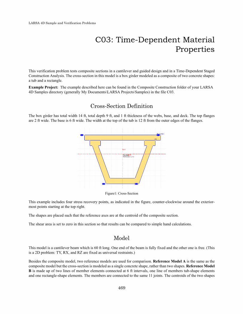
LARSA 4D Sample and Verification Problems
C03: Time-Dependent MaterialProperties
This verification problem tests composite sections in a cantilever and guided design and in a Time-Dependent StagedConstruction Analysis. The cross-section in this model is a box girder modeled as a composite of two concrete shapes:a tub and a rectangle.
Example Project: The example described here can be found in the Composite Construction folder of your LARSA4D Samples directory (generally My Documents\LARSA Projects\Samples) in the file C03.
Cross-Section DefinitionThe box girder has total width 14 ft, total depth 9 ft, and 1 ft thickness of the webs, base, and deck. The top flangesare 2 ft wide. The base is 6 ft wide. The width at the top of the tub is 12 ft from the outer edges of the flanges.
Figure1: Cross-Section
This example includes four stress recovery points, as indicated in the figure, counter-clockwise around the exterior-most points starting at the top right.
The shapes are placed such that the reference axes are at the centroid of the composite section.
The shear area is set to zero in this section so that results can be compared to simple hand calculations.
ModelThis model is a cantilever beam which is 60 ft long. One end of the beam is fully fixed and the other one is free. (Thisis a 2D problem: TY, RX, and RZ are fixed as universal restraints.)
Besides the composite model, two reference models are used for comparison. Reference Model A is the same as thecomposite model but the cross-section is modeled as a single concrete shape, rather than two shapes. Reference ModelB is made up of two lines of member elements connected at 6 ft intervals, one line of members tub-shape elementsand one rectangle-shape elements. The members are connected to the same 11 joints. The centroids of the two shapes
469

LARSA 4D Sample and Verification Problems
are offset from the joints by offsetting the shapes from the reference axis in Section Composer. This is shown for thetub section in the figure below:
Figure2: Cross-Section of tub
The members all have an orientation angle of 90 degrees.
To activate time-dependent material effects, a Material Time Effect record is added to the project in the Propertiesspreadsheets. It does not need to be configured for CEB-FIP90, which we will use. This record is then assigned to theFC_4 material record in the More Properties section of the Materials spreadsheet. Additionally, ensure that FC_4 ismarked as “Normal” under Concrete Cement Hardening Type . Its Fc_28 is 4 kip/in2. The default relative humidityis left at 80% in the Construction Stages . In Analysis → Time Dependent Analysis Options , set the code to CEB-FIP 90 and turn on Time Effect on Elastic Modulus, Creep, and Shrinkage and turn off all other time-dependentmaterial effects.
The construction sequence consists of four steps:
Stage1: Day5 - Cast the concrete of the tub.
Stage2: Day10 - Cast the concrete of the deck.
Stage3: Day15 - a) Assemble the tub. b) Tub self-weight is applied.
Stage4: Day25 - a) Assemble the deck. b) Deck self-weight is applied.
Besides these steps, additional construction stages are placed on days 50, 100, 400, and 1000. These stages have noactivities but are used to compute the long-term effects of creep.
Cross-Sectional PropertiesA summary of the computation of cross-sectional properties is given below. Since the cross-section has a singlematerial, the modulus of elasticity of concrete is not relevant. In the tables below, yc is the distance from a shapecentroid to the composite centroid.
Computation of the composite cross-section centroid
470

LARSA 4D Sample and Verification Problems
yc (ft) A (ft2)
Tub -1.83 23.1
Deck 3.02 14.0
Computation of compound properties
Tub Deck Composite
Base Transformed Base Transformed
A (ft2) 23.1 --- 14.0 --- 37.1
Izz (ft4) 163 240 1.17 129 369
J (ft4) 7.84 --- 4.44 --- 580
LARSA 4D’s computations match the hand calculation to within rounding error. There is no hand verification for thetorsion constant J at this time.
Self-Weight LoadingThe results of a static self-weight load case are reported below, as well as a hand calculation using
δ = WL4/8EI
The unit weight of concrete is taken as 0.15 kip/ft3.
Deflection at free end
Deflection (ft)
Hand Calc. 0.047
Composite 0.047
Reference A 0.047
Reference B 0.047
The same method will be used to verify stresses as in C01: Single Span with Roller under Vertical Load (page 453). Thestress at the left end of the cantilever is
σ = yWL2/2I
where y is the fiber location relative to the centroid. Stress point 1 is at the top of the deck and stress point 3 is atthe bottom of the tub.
Stresses
471
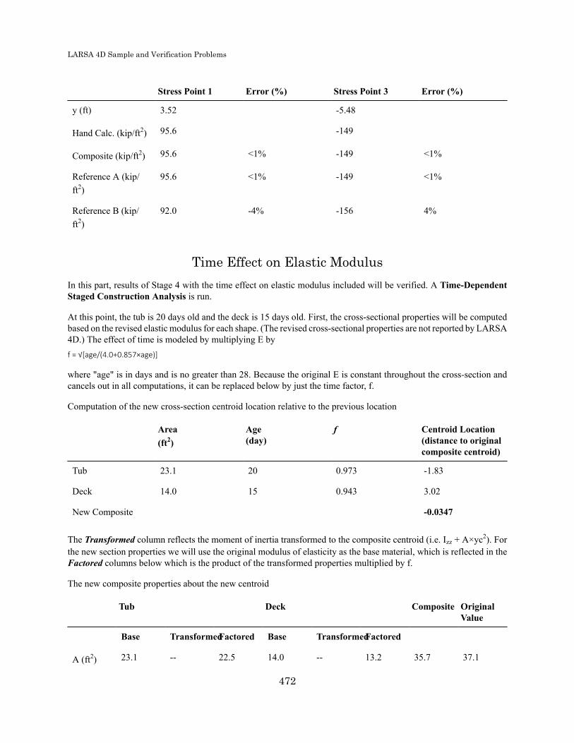
LARSA 4D Sample and Verification Problems
Stress Point 1 Error (%) Stress Point 3 Error (%)
y (ft) 3.52 -5.48
Hand Calc. (kip/ft2) 95.6 -149
Composite (kip/ft2) 95.6 <1% -149 <1%
Reference A (kip/ft2)
95.6 <1% -149 <1%
Reference B (kip/ft2)
92.0 -4% -156 4%
Time Effect on Elastic ModulusIn this part, results of Stage 4 with the time effect on elastic modulus included will be verified. A Time-DependentStaged Construction Analysis is run.
At this point, the tub is 20 days old and the deck is 15 days old. First, the cross-sectional properties will be computedbased on the revised elastic modulus for each shape. (The revised cross-sectional properties are not reported by LARSA4D.) The effect of time is modeled by multiplying E byf = √[age/(4.0+0.857×age)]
where "age" is in days and is no greater than 28. Because the original E is constant throughout the cross-section andcancels out in all computations, it can be replaced below by just the time factor, f.
Computation of the new cross-section centroid location relative to the previous location
Area(ft2)
Age(day)
f Centroid Location(distance to originalcomposite centroid)
Tub 23.1 20 0.973 -1.83
Deck 14.0 15 0.943 3.02
New Composite -0.0347
The Transformed column reflects the moment of inertia transformed to the composite centroid (i.e. Izz + A×yc2). Forthe new section properties we will use the original modulus of elasticity as the base material, which is reflected in theFactored columns below which is the product of the transformed properties multiplied by f.
The new composite properties about the new centroid
Tub Deck Composite OriginalValue
Base TransformedFactored Base TransformedFactored
A (ft2) 23.1 -- 22.5 14.0 -- 13.2 35.7 37.1
472

LARSA 4D Sample and Verification Problems
Tub Deck Composite OriginalValue
Izz (ft4) 163 237 231 1.17 132 124 356 369
In Step 4 the deck is constructed and its self weight is applied. The incremental displacements at the far end of thecantilever are given in the table below, along with a hand calculation (δ = WL4/8EI, W=2.1kip/ft) and, for comparison,a hand calculation for a similar model with the original day-28 properties.
Reference Model A is not applicable in this comparison because it could only be assembled in one step, as it is madeof a single shape, and therefore could not have self-weight applied for just one shape in this step.
Deflection at free end (Incremental)
Deflection (ft) Error (%)
Hand Calc. 0.0184
Composite 0.0184 <1%
Reference B 0.0185 <1%
Day 28 Hand Calc. 0.0178
Similar method will be used to verify stresses as in previous sections. Now that the two shapes have different materialproperties, the member-end moment
M = WL2/2
must be converted to a curvature first
κ = WL2/2EI
using the composite Izz and the corresponding original (28-day) E. The curvature is multiplied by the fiber location yand the 15- or 20-day modulus of elasticity at the fiber to find the stress. The fiber locations of the stress points arechanged here to reflect the new centroid location. Hand calculations assuming all 28-day concrete is also provided forcomparison. Stress point 1 is at the top of the deck and stress point 3 is at the bottom of the tub.
Stresses (Incremental)
Stress Point 1 Stress Point 3
y (ft) 3.55 -5.44
Hand Calc. (kip/ft2)
(yfWL2/2I)
35.5 -56.2
Composite (kip/ft2) 35.7 -56.3
Reference B (kip/ft2) 36.0 -58.8
Day 28 Hand Calc. (kip/ft2) 36.1 -56.0
473

LARSA 4D Sample and Verification Problems
ShrinkageTo verify shrinkage, total effect on stress of shrinkage though day 400 will be checked. Shrinkage, εs as given belowaccording to CEB-FIP90, is an additional strain added into the cross-section accumulated from time t0 to time t1. Inthis part, the time effect on elastic modulus is not included.εs = εcs0[βs(t1) - βs(t0)]
εcs0 = (160 + 10×βsc×(9-Fc28/10))/1e6 × (-1.55×(1.0-(RH/100)3))
βs(t) = sqrt((t-TS) / (350×((H/100)2) + (t-TS)))
where TS = 3, βsc = 5, H = 2 × Area/Perimeter converted to millimeters, RH is the relative humidity (80%), and t0, t1are the ages of the section in days. Fc28 = 27.6 MPa (576 kip/ft2).
The shrinkage must be computed in two parts. From days 15 to 25, the tub alone is constructed. The shrinkage resultsin deformation due to pure strain but neither bending nor stress. From days 25 to 400, the tub and the deck are subjectto different amounts of shrinkage. Because the shapes are connected, this creates bending strain and eigenstresses.Additionally, strain compatibility must be considered. Because of “plane sections remain plane,” shrinkage must beconsidered as the sum of two virtual strain components.
The first component called the “external” component, with magnitude εs, and is responsible for causing deformation.In Ghali, Favre, and Elbadry (2002) example 5.2, this corresponds to the forces and moments that undo the artificialrestraint on shrinkage. The second or “internal” component has magnitude -εs but does not cause deformation. (Itcorresponds to Ghali, Favre, and Elbadry’s strain in the section when shrinkage is restrained.) Initially, the externaland internal virtual strains cancel out.
Next replace the external strain with an equivalent force and moment at the beam end. The external stresses areintegrated across the cross-section to determine an equivalent forceF = εs×E×A
and momentM = F×yc
imposed at the beam end, which in turn determines the actual deformation of the beam as the combination of pureεp=F/EA
and rotationalεr=M/EI
strains (E, A, and I are properties of the entire cross-section, with E unmodified for time). In this way, the originalexternal strains which have sharp changes at the boundaries of shapes are turned into a linear strain profile across theentire cross-section, which satisfies strain compatibility (i.e. plane sections remain plane).
The table below shows the relevant computations for the external virtual strain. The perimeters used in the handcalculation include the interior perimeter of the tub and the unexposed perimeters at the interface of the two shapesin order to match the computations in LARSA 4D.
Because the original external strains are constant throughout each individual shape, a lumped force at each shape’scentroid,F = εsEA
is given in the table below in order to compute the moment about the cross-section centroid.
Computation of External Strain, Day 400474

LARSA 4D Sample and Verification Problems
Tub Deck
Area (ft2) 23.1 14.0
Perimeter (ft) 48.1 30
Age on Day 15 (day) 10 n/a (no stiffness)
Age on Day 25 (day) 20 15
Shrinkage (εs1), days 15-25 -9.57e-6 n/a
Age on Day 400 (day) 395 390
Shrinkage (εs2), days 25-400 -9.46e-5 -1.01e-4
Equivalent Force F= εs2EA (kip) -1,134 -734
cy (ft) -1.83 3.02
Equivalent Moment M = Fcy (kip-ft)
2076 -2217
Total Pure Strain (εp=F/EA + εs1) -1.07e-4 -1.07e-4
Total Rotational Strain (εr=M/EI)(per ft)
-7.4e-7 -7.4e-7
The deformation of the centroid of the span is circular with a radius of curvature r equal to the reciprocal of the totalrotational strain. At the same time, the arc-length of the span, s, is reduced according to the pure strain, therefores = 60×(1+εp)
A hand computation for displacement (∆x, ∆y) is explained in the diagram below.θ = s/r
x1 = r×cos(π/2 – θ)
y1 = r×sin(π/2 – θ)
∆x = x1 - 60
∆y = r – y1
475

LARSA 4D Sample and Verification Problems
Figure3: Deformed Shape due to Shrinkage
The displacement at the free end of the cantilever is given in the table below, from hand calculations and as reportedby LARSA 4D in the composite model and the two reference models. In LARSA 4D, Extract Shrinkage is used toreport the cumulative effects of shrinkage alone.
Displacement
∆x (ft) ∆y (ft)
Hand Calc. -6.38e-3 1.26e-3
Composite -6.38e-3 1.25e-3
Reference A -5.74e-3 0.00
Reference B -6.38e-3 1.25e-3
The stress in any fiber is then given essentially byσ = E×((εp-εs1) +y×εr - εs2)
the sum of the external and internal components of stress at each fiber. For stresses we subtract εs1 from εp in theexternal component of stress because when the tub alone is constructed shrinkage does not create stress. Similarly, itis not included in the internal component of stress. Stresses at the free end of the cantilever are given below.
476

LARSA 4D Sample and Verification Problems
Stresses
Stress Point 1 Stress Point 3
y (ft) 3.52 -5.47
Hand Calc. (kip/ft2) 0.688 0.791
Composite (kip/ft2) 0.691 0.790
Reference A (kip/ft2) 0.00 0.00
Reference B (kip/ft2) 0.691 0.79
CreepThe computation of creep is significantly more complex than that of shrinkage, and creep involves an integration ofstresses over time. Rather than presenting a hand calculation, simply compare the results of the composite model tothe two reference models.
Recall that Reference A is a single-member representation of the composite model in which the whole section is caston day 5. This differs from the composite model and Reference B in which the two shapes are cast at different times.
The cumulative effect of creep alone on day 1000 (i.e. “extract creep”) is reported in the table below. Jointdisplacements in vertical direction at the far end of the cantilever and stresses at the fixed end are reported. As inprevious models, we expect joint displacements in the composite model and Reference B to match exactly but weexpect non-composite models to report different stresses due to the distribution of forces in the rigid connections notpresent in the composite model.
Stresses
Displacement
(ft)
Stress Point 1
(kip/ft2)
Stress Point 3
(kip/ft2)
Composite -0.097 63.6 55.2
Reference A -0.094 0.00 0.00
Reference B -0.097 55.6 49.0
ReferencesGhali, A., Favre, R., and Elbadry, M. Conctrete Structures: Stresses and Deformations: Analysis and Design forServiceability (2002).
477

LARSA 4D Sample and Verification Problems
478
LARSA 4D Sample and Verification Problems
C04: Thermal Loads
This verification problem tests composite sections for uniform, linear, and nonlinear thermal gradients in a linear staticanalysis.
Example Project: The example described here can be found in the Composite Construction folder of your LARSA4D Samples directory (generally My Documents\LARSA Projects\Samples) in the file C04.
Cross-Section DefinitionThe cross-section definition is the same in problems C01: Single Span with Roller under Vertical Load (page 453) andC02: Staged Construction Analysis (page 461). The cross-section used in this problem is composed of a steel I-shape anda concrete slab on top. The dimensions are:
• I-Shape: 5 ft deep; 2 ft wide; 0.2 ft flange and web thickness
• Rectangle Shape: 0.8 ft deep; 4 ft wide
This example includes six Stress Recovery Points: 1-4 clockwise around the I-shape, and 5-6 at the upper-right andupper-left of the concrete slab, respectively.
479

LARSA 4D Sample and Verification Problems
Figure1: Cross-Section
The shapes are placed such that the reference axes are at the centroid of the deck slab.
The properties for the section as a whole, with concrete as the reference material, are given in the table below.
Section Properties
A (ft2) 17.0
Iyy (ft4) 6.44
480
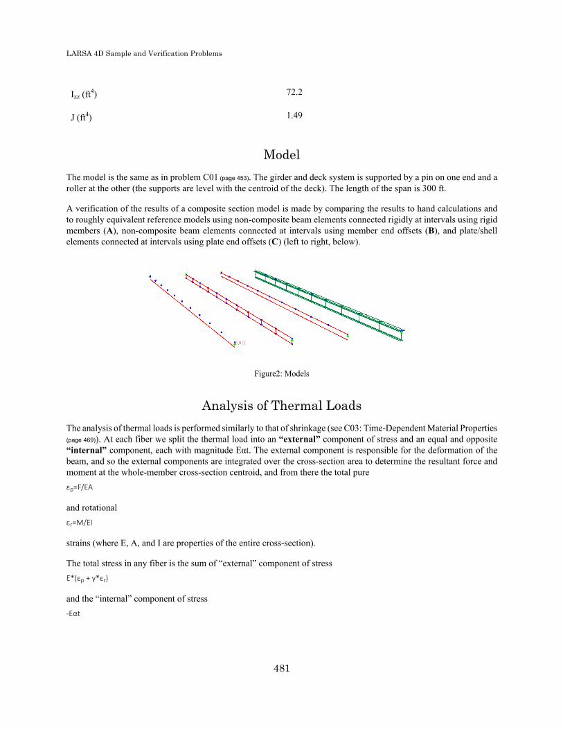
LARSA 4D Sample and Verification Problems
Izz (ft4) 72.2
J (ft4) 1.49
ModelThe model is the same as in problem C01 (page 453). The girder and deck system is supported by a pin on one end and aroller at the other (the supports are level with the centroid of the deck). The length of the span is 300 ft.
A verification of the results of a composite section model is made by comparing the results to hand calculations andto roughly equivalent reference models using non-composite beam elements connected rigidly at intervals using rigidmembers (A), non-composite beam elements connected at intervals using member end offsets (B), and plate/shellelements connected at intervals using plate end offsets (C) (left to right, below).
Figure2: Models
Analysis of Thermal LoadsThe analysis of thermal loads is performed similarly to that of shrinkage (see C03: Time-Dependent Material Properties(page 469)). At each fiber we split the thermal load into an “external” component of stress and an equal and opposite“internal” component, each with magnitude Eαt. The external component is responsible for the deformation of thebeam, and so the external components are integrated over the cross-section area to determine the resultant force andmoment at the whole-member cross-section centroid, and from there the total pureεp=F/EA
and rotationalεr=M/EI
strains (where E, A, and I are properties of the entire cross-section).
The total stress in any fiber is the sum of “external” component of stressE*(εp + y*εr)
and the “internal” component of stress-Eαt
481

LARSA 4D Sample and Verification Problems
Uniform Thermal LoadThis section verifies the uniform thermal load. A uniform +20 °F thermal change is applied to the entire cross-section.Steel has a larger coefficient of thermal expansion. Thus we expect the steel I shape, which is below the compositecentroid, to cause the entire model to have an upward curvature. Because of the vertical supports at the ends, therewill be negative vertical displacements along the model.
Vertical Displacements. Units are ft
@ 20% @ Mid-Span
Composite -0.0150 -0.0235
Reference A -0.0150 -0.0235
Reference B -0.0150 -0.0235
Reference C -0.0456 -0.0292
Since plane sections remain plane, the deformation of the two shapes that make up the composite section must berelated. The steel part is restrained from expanding as much as it would unrestrained, so we should expect a compressivestress at the centroid of the steel shape. Similarly, we expect a tensile stress at the centroid of the concrete shape.
The integration of the “external” component of stress is given in the following table. The moment and rotational strainare at the compound centroid.
Steel I Concrete Slab
E (kip/ft2) 4,176,000 519,120
A (ft2) 1.72 3.2
α (1/°F) 6.5e-6 5.5e-6
Force (αTEA) (kip) 933.8 182.7
Centroid Loacation (ft) -0.544 2.356
Moment (kip-ft) -508.0 -430.5
Total Pure Strain (εp) -1.262e-4 -1.262e-4
Total Rotational Strain (εr) (per ft) -2.069e-6 -2.069e-6
The total stress in each shape is computed in the following table by summing the internal and external components ofstress. Note that stress recovery point 3 is in the steel shape and stress recovery point 5 is in the concrete shape andso each stress recovery point uses a different E value.
I Shape Centroid Slab Centroid Stress Point 3 Stress Point 5
y (ft) -0.544 2.356 -3.044 2.756
E*(εp+y*εr) (kip/ft2) 532 63.0 553.3 62.54
482

LARSA 4D Sample and Verification Problems
I Shape Centroid Slab Centroid Stress Point 3 Stress Point 5
-αTE (kip/ft2) -543 -57.1 -543 -57.1
Total Stress (kips/ft2)
-11.2 5.88 10.4 5.44
Stresses. Units are kip/ft2.
Stress Point 3 Error (%) Stress Point 5 Error (%)
Composite 10.9 5% 5.44 0%
Reference A 10.9 5% 5.44 0%
Reference B 10.9 5% 5.44 0%
Reference C 23.5 - 13.12 -
Linear Gradient Thermal LoadThis section verifies the linear gradient thermal load. A thermal change is applied to the entire cross-section with a T0= +20 °F change at the cross-section centroid and a Tslope = 5 °F/ft slope in the vertical axis. (That results in a temperatechange of +4.8 °F at the bottom of the steel I shape, 29.8 °F at the meeting of the two shapes, and 33.8 °F at the top ofthe concrete slab.) A linear thermal gradient cannot be applied in the plate-based reference model because a thermalload cannot be entered to vary along the plate’s surface.
In the non-composite reference models, the linear thermal load is broken down into a part for the I shape member anda part for the slab member.
Displacements
@ 20% @ Mid-Span
Composite (ft) 0.210 0.328
Reference A (ft) 0.210 0.328
Reference B (ft) 0.210 0.328
To compute the “external” component of stress at the composite cross-section centroid, the stress at each fiber Eαtis integrated over the area of the section, i.e.F = ∫ Eaαa(20+5y)da
andM = ∫ Eaαay(20+5y)da
where Ea and αa are the elastic modulus and coefficient of thermal expansion of fiber a, and y is the location of thefiber relative to the centroid of the composite section. This can be computed by breaking the cross-section down intoits rectangular pieces which have constant E, α, and y for each horizontal strip with width w, so thatF = ∑rect wEα∫(20+5y)dy
483

LARSA 4D Sample and Verification Problems
M = ∑rect wEα∫ y(20+5y)dy
Computation of “External” Force and Moment
RectangularPart
y0 (ft) y1 (ft) width (w)(ft)
E (kip/ft2) α (1/°F) F (kip) M (kip-ft)
BottomFlange
0.0 0.2 2.0 4,176,000 6.5e-6 57.6 -169
Web 0.2 4.8 0.2 4,176,000 6.5e-6 432 -14.8
Top Flange 4.8 5.0 2.0 4,176,000 6.5e-6 318 590
Slab 5.0 5.8 4.0 519,120 5.5e-6 290 686
The sum of the forces and moments at the section centroid and the corresponding total pure strainεp = F/EA
and rotational strainεr = M/EI
(with E and I here the properties of the cross-section) are given below.
Computation of “External” Force and Moment
F (kip) 1098
M (kip-ft) 1093
εp 1.24e-4
εr 2.92e-5
The total stress in each shape is computed in the following table by adding the “external” stress as given by the totalstrains above and the “internal” stress based on the value of the linear curve at the fiber. Note that stress recoverypoint 3 is in the steel shape and stress recovery point 5 is in the concrete shape and have E and α set accordingly. They values are relative to the cross-section centroid.
Hand Calculation of Stress
Stress Point 3 Stress Point 5
y (ft) -3.044 2.756
E*(εp+y*εr) (kip/ft2) 147 106
-αE(T0+y*Tslope) (kip/ft2) -130 -96.5
Total Stress (kips/ft2) 16.2 9.63
Stresses. Units are kip/ft2
484
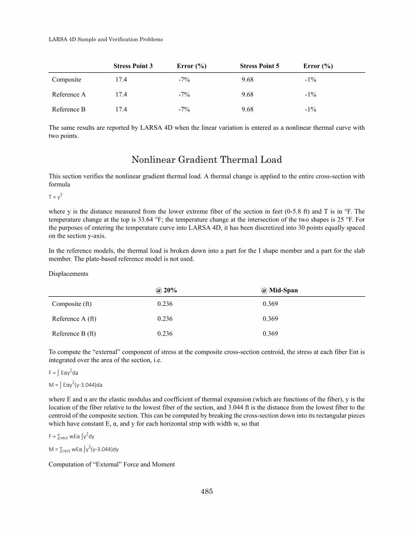
LARSA 4D Sample and Verification Problems
Stress Point 3 Error (%) Stress Point 5 Error (%)
Composite 17.4 -7% 9.68 -1%
Reference A 17.4 -7% 9.68 -1%
Reference B 17.4 -7% 9.68 -1%
The same results are reported by LARSA 4D when the linear variation is entered as a nonlinear thermal curve withtwo points.
Nonlinear Gradient Thermal LoadThis section verifies the nonlinear gradient thermal load. A thermal change is applied to the entire cross-section withformula
T = y2
where y is the distance measured from the lower extreme fiber of the section in feet (0-5.8 ft) and T is in °F. Thetemperature change at the top is 33.64 °F; the temperature change at the intersection of the two shapes is 25 °F. Forthe purposes of entering the temperature curve into LARSA 4D, it has been discretized into 30 points equally spacedon the section y-axis.
In the reference models, the thermal load is broken down into a part for the I shape member and a part for the slabmember. The plate-based reference model is not used.
Displacements
@ 20% @ Mid-Span
Composite (ft) 0.236 0.369
Reference A (ft) 0.236 0.369
Reference B (ft) 0.236 0.369
To compute the “external” component of stress at the composite cross-section centroid, the stress at each fiber Eαt isintegrated over the area of the section, i.e.
F = ∫ Eαy2da
M = ∫ Eαy2(y-3.044)da
where E and α are the elastic modulus and coefficient of thermal expansion (which are functions of the fiber), y is thelocation of the fiber relative to the lowest fiber of the section, and 3.044 ft is the distance from the lowest fiber to thecentroid of the composite section. This can be computed by breaking the cross-section down into its rectangular pieceswhich have constant E, α, and y for each horizontal strip with width w, so that
F = ∑rect wEα ∫y2dy
M = ∑rect wEα ∫y2(y-3.044)dy
Computation of “External” Force and Moment
485
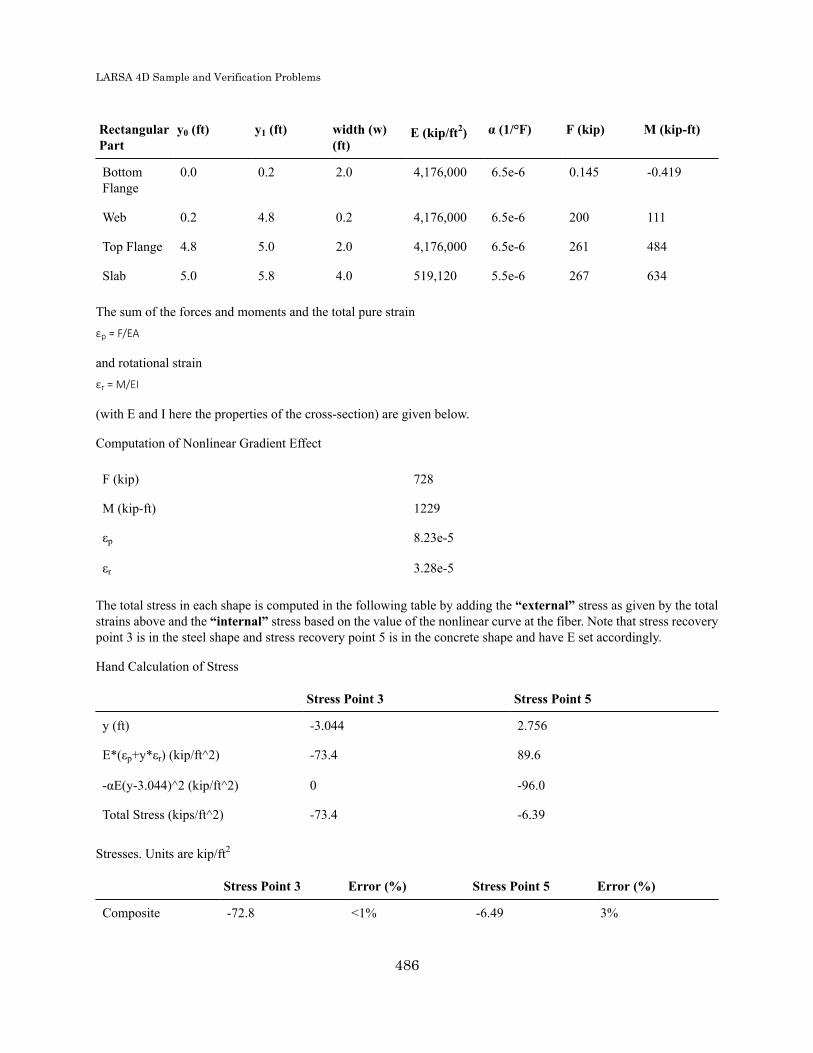
LARSA 4D Sample and Verification Problems
RectangularPart
y0 (ft) y1 (ft) width (w)(ft)
E (kip/ft2) α (1/°F) F (kip) M (kip-ft)
BottomFlange
0.0 0.2 2.0 4,176,000 6.5e-6 0.145 -0.419
Web 0.2 4.8 0.2 4,176,000 6.5e-6 200 111
Top Flange 4.8 5.0 2.0 4,176,000 6.5e-6 261 484
Slab 5.0 5.8 4.0 519,120 5.5e-6 267 634
The sum of the forces and moments and the total pure strainεp = F/EA
and rotational strainεr = M/EI
(with E and I here the properties of the cross-section) are given below.
Computation of Nonlinear Gradient Effect
F (kip) 728
M (kip-ft) 1229
εp 8.23e-5
εr 3.28e-5
The total stress in each shape is computed in the following table by adding the “external” stress as given by the totalstrains above and the “internal” stress based on the value of the nonlinear curve at the fiber. Note that stress recoverypoint 3 is in the steel shape and stress recovery point 5 is in the concrete shape and have E set accordingly.
Hand Calculation of Stress
Stress Point 3 Stress Point 5
y (ft) -3.044 2.756
E*(εp+y*εr) (kip/ft^2) -73.4 89.6
-αE(y-3.044)^2 (kip/ft^2) 0 -96.0
Total Stress (kips/ft^2) -73.4 -6.39
Stresses. Units are kip/ft2
Stress Point 3 Error (%) Stress Point 5 Error (%)
Composite -72.8 <1% -6.49 3%
486

LARSA 4D Sample and Verification Problems
Stress Point 3 Error (%) Stress Point 5 Error (%)
Reference A -73.1 1% -6.39 1%
Reference B -73.1 1% -6.39 1%
487

LARSA 4D Sample and Verification Problems
488

LARSA 4D Sample and Verification Problems
Samples for Buckling Analysis
These samples provide an overview of linear and nonlinear buckling analysis.
For More Information, please refer to the following documentation.
• For help on nonlinear buckling analysis, see Nonlinear Buckling Analysis in LARSA 4D Reference Manual.
B01: Torsional Buckling of Crucifix Section with Shell Elements 491Problem Description 491Solution Comparison 492References 492
B02: Lateral Buckling of I Section with Shell Elements 493Problem Description 493Solution Comparison 494References 494
B03: Lateral Torsional Buckling of C Section with Shell Elements 495Problem Description 495Solution Comparison 496References 496
489

LARSA 4D Sample and Verification Problems
490

LARSA 4D Sample and Verification Problems
B01: Torsional Buckling of CrucifixSection with Shell Elements
A fixed-fixed girder with a crucifix cross-section is modeled with nonlinear shell elements. The girder is subjected toan incrementally increasing axial load. Determine the torsional buckling load by analyzing the model with NonlinearBuckling Analysis.
Example Project: The example described here can be found in the Buckling folder of your LARSA 4D Samplesdirectory (generally My Documents\LARSA Projects\Samples) in the file B01.
Problem Description
Fixed-Fixed girder and its cross-section
The girder consists of 160 nonlinear shell elements. Each blade of the section is 40 shells. All the translational androtational degrees of freedom are restrained for the joints at the left end of the section. For the right end of the section,only axial translation is free to see the behavior of the section under axial loading.
The blades of the cross-section have 0.4 in. thickness and 8 in. width. The total length of the girder is 100 inches.
The material has 21,000 kips/in2 elastic modulus with 0.3 Poisson's ratio.
In order to achieve nonlinear behavior, the MITC4 element formulation is used.
A small 1 kip-in perturbation is applied at the middle of the cross-section as a small torsional load to initiate the twisting.Loading is applied axially by gradually increasing it until it reaches 580 kips. At every step, the load is increased by20 kips. It is modeled as a 1 kip load divided equally across the 5 nodes at the tip of each blade and the node at theintersection of the blades at the free end of the member. Perturbation and loading are defined in separate load cases.Each step is created as a load combination. Perturbation is only applied in first load combination. The axial load isapplied in each step by increasing its magnitude 20 times. The model is analyzed using Nonlinear Buckling Analysis.
491

LARSA 4D Sample and Verification Problems
Solution Comparison
The results are obtained from the axial loading versus twisting angle (Rx of 26th joint) curve of the model. The loadwhere the rate of the curve changes remarkably may be counted as buckling load. In order to compare the results, theindependent solution which is given by Timoshenko and Gere based on Bernoulli beam theory with Vlasov warpingis shown in the graph.
Load deflection curve
References• S.P. Timoshenko, J.M. Gere, Theory of Elastic Stability, second ed., McGraw-Hill, Tokyo, 1961
For More Information, please refer to the following documentation.
• For help on nonlinear buckling analysis, see Nonlinear Buckling Analysis in LARSA 4D Reference Manual.• For help on nonlinear plate elements, see Plates in LARSA 4D Reference Manual.
492
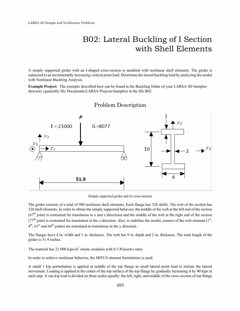
LARSA 4D Sample and Verification Problems
B02: Lateral Buckling of I Sectionwith Shell Elements
A simply supported girder with an I-shaped cross-section is modeled with nonlinear shell elements. The girder issubjected to an incrementally increasing vertical point load. Determine the lateral buckling load by analyzing the modelwith Nonlinear Buckling Analysis.
Example Project: The example described here can be found in the Buckling folder of your LARSA 4D Samplesdirectory (generally My Documents\LARSA Projects\Samples) in the file B02.
Problem Description
Simple supported girder and its cross-section
The girder consists of a total of 960 nonlinear shell elements. Each flange has 320 shells. The web of the section has320 shell elements. In order to obtain the simply supported behavior, the middle of the web at the left end of the section(67th joint) is restrained for translation in x and z directions and the middle of the web at the right end of the section(77th joint) is restrained for translation in the z direction. Also, to stabilize the model, corners of the web element (1st,4th, 61st and 64th joints) are restrained in translation in the y direction.
The flanges have 4 in. width and 1 in. thickness. The web has 9 in. depth and 2 in. thickness. The total length of thegirder is 51.9 inches.
The material has 21,000 kips/in2 elastic modulus with 0.3 Poisson's ratio.
In order to achieve nonlinear behavior, the MITC4 element formulation is used.
A small 1 kip perturbation is applied at middle of the top flange as small lateral point load to initiate the lateralmovement. Loading is applied at the center of the top surface of the top flange by gradually increasing it by 40 kips ineach step. A one kip load is divided on three nodes equally: the left, right, and middle of the cross-section of top flange
493

LARSA 4D Sample and Verification Problems
at the middle end of the member. Perturbation and loading are defined in separate load cases. Each step is created asa load combination. Perturbation is only applied in first load combination. The vertical point load is applied in eachstep by increasing its magnitude 40 times. The model is analyzed using Nonlinear Buckling Analysis.
Solution Comparison
The results are obtained from axial loading versus lateral displacement of top flange(Ty of joint 31st) curve of themodel. The load where the rate of the curve changes remarkably may be counted as buckling load. In order to comparethe results, the independent solution which is given by Timoshenko and Gere is shown in the graph.
Load deflection curve
References• S.P. Timoshenko, J.M. Gere, Theory of Elastic Stability, second ed., McGraw-Hill, Tokyo, 1961
For More Information, please refer to the following documentation.
• For help on nonlinear buckling analysis, see Nonlinear Buckling Analysis in LARSA 4D Reference Manual.• For help on nonlinear plate elements, see Plates in LARSA 4D Reference Manual.
494

LARSA 4D Sample and Verification Problems
B03: Lateral Torsional Buckling of CSection with Shell Elements
A cantilever girder with a C-shaped cross-section is modeled with nonlinear shell elements. The girder is subjectedto an incrementally increasing vertical tip load. Determine the lateral-torsional buckling load by analyzing the modelwith Nonlinear Buckling Analysis.
Example Project: The example described here can be found in the Buckling folder of your LARSA 4D Samplesdirectory (generally My Documents\LARSA Projects\Samples) in the file B03.
Problem Description
Cantilever girder and its cross-section
The girder consists of a total of 640 nonlinear shell elements. Each flange has 160 shells. The web of the section has320 shell elements. In order to obtain the cantilever behavior, the corners of the top and bottom flanges at the left endof the girder (1st, 2nd, 3rd and 4th joints) are fixed in both translation and rotation. Joints at the right end of the girderare free to rotate and translate.
Flanges have 10 in. width and 1.6 in. thickness. The web has 26.8 in. depth and 1 in. thickness. The total length ofthe girder is 900 inches.
The material has 21,000 kips/in2 elastic modulus with 0.3 Poisson's ratio.
In order to achieve nonlinear behavior, the MITC4 element formulation is used.
Loading is applied where the web element and the bottom flange coincides at the free end of the girder vertically bygradually increasing until it reaches 24 kips. Each step is created as a load combination. Vertical load is applied in eachstep. The model is analyzed by using Nonlinear Buckling Analysis.
495

LARSA 4D Sample and Verification Problems
Solution Comparison
The results are obtained from axial loading versus vertical displacement of free end (Tz of joint 287th) curve of themodel. The load where the rate of the curve changes remarkably may be counted as buckling load. In order to comparethe results, the independent solution which is given by Gruttmann is shown in the graph.
Load deflection curve
References• R. Gruttmann, R. Sauer, W. Wagner, Theory and numerics of three-dimensional beams with elastoplastic
behaviour, Int. J.Numer. Methods Engrg. 48 (2000) 1675–1702.
For More Information, please refer to the following documentation.
• For help on nonlinear buckling analysis, see Nonlinear Buckling Analysis in LARSA 4D Reference Manual.• For help on nonlinear plate elements, see Plates in LARSA 4D Reference Manual.
496
LARSA 4D Sample and Verification Problems
Index
arch, 169barrel vault, 45beams, 195bridge path, 329buckling, 489cable roof, 163cables, 157cantilever
E01: Triangular Cantilever Plate Eigenvalues, 187E02: Square Cantilever Plate Eigenvalues, 191
circular arch, 169circular plate, 39composite construction
C01: Single Span with Roller under Vertical Load, 453C02: Staged Construction Analysis, 461C03: Time-Dependent Material Properties, 469C04: Thermal Loads, 479Samples for Composite Construction, 451
compression-only foundation springs, 159concentrated mass, 233cylindrical roof, 45diamond shaped frame, 165dynamic loads, 233eigenvalue analysis, 185elastic foundation
L03: Beam on Elastic Foundation, 19N03: Beam on an Elastic Soil Foundation, 159
element space truss, 25geometric nonlinearity
N06: Diamond Shaped Frame - Geometric Nonlinear, 165N08: A High Arch Structure - Geometric Nonlinear, 169
geometric stiffeningL10: Tie Beam without Geometric Stiffening, 37N01: Tie Beam with Geometric Stiffening, 155
hemispherical shell, 41holes, 39influence lines and surfaces, 321linear elastic static, 11linear gradient thermal load, 479linear time history analysis, 229live load analysis, 321lumped masses, 203mass elements, 203nonlinear elastic static, 153nonlinear gradient thermal load, 479nonlinear thermal load, 51nonlinear time history analysis, 229pin connection
L02: Beam with Elastic Supports, 17L06: Static Analysis of a Space Frame, 29
plateB01: Torsional Buckling of Crucifix Section with Shell Elements, 491
497

LARSA 4D Sample and Verification Problems
B02: Lateral Buckling of I Section with Shell Elements, 493B03: Lateral Torsional Buckling of C Section with Shell Elements, 495N13: Straight Cantilever Girder with Nonlinear Shell Elements in Membrane Action, 173N14: Straight Cantilever Girder with Nonlinear Shell Elements in Plate Action, 177N15: Slit Annular Plate with Vertical Load, 181
plate thermal loads, 33plates
E01: Triangular Cantilever Plate Eigenvalues, 187E02: Square Cantilever Plate Eigenvalues, 191L07: Plate Thermal Analysis, 33L08: Shell-Bending of a Tapered Cantilever, 35L11: Circular Plate with a Hole Static Analysis, 39
point loadsL02: Beam with Elastic Supports, 17L06: Static Analysis of a Space Frame, 29
reactions, 157reinforced concrete, 45response spectra analysis, 219settlement, 49simply supported beam, 19space truss, 25span break markers, 329spring mass system, 231springs, 203staged construction analysis
C02: Staged Construction Analysis, 461Samples for Staged Construction Analysis, 261
steel bridge, 339stressed eigenvalue analysis, 215tapered cantilever, 35temperature loads
L14: 2D Truss - Thermal Loads and Settlement, 49L16: Nonlinear Thermal Load, 51
tensile force, 155tension, 157thermal loads
C04: Thermal Loads, 479L05: 2D Truss with Thermal Load, 27L14: 2D Truss - Thermal Loads and Settlement, 49L16: Nonlinear Thermal Load, 51
tie beamL10: Tie Beam without Geometric Stiffening, 37N01: Tie Beam with Geometric Stiffening, 155
time history analysis, 229time-dependent material properties, 469time-dependent staged-construction analysis, 469torsional system, 213truss
L01: 2D Truss with Static Loads, 15L05: 2D Truss with Thermal Load, 27L14: 2D Truss - Thermal Loads and Settlement, 49
uniform lateral loadL10: Tie Beam without Geometric Stiffening, 37N01: Tie Beam with Geometric Stiffening, 155
uniform load, 19uniform loads, 45uniform thermal load, 479yielding elastic supports
498

LARSA 4D Sample and Verification Problems
L02: Beam with Elastic Supports, 17L06: Static Analysis of a Space Frame, 29
499
Copyright © 2022 FDOKUMEN