3D interpolation of grain size distributions in the upper 5m of the channel bed of three lower Rhine...

www.elsevier.com/locate/pce

Physics and Chemistry of the Earth 30 (2005) 303–316

3D interpolation of grain size distributions in the upper 5 mof the channel bed of three lower Rhine distributaries

S.H.L.L. Gruijters *, D. Maljers, J.G. Veldkamp

Netherlands Institute of Applied Geosciences, TNO Geology Division, P.O. Box 80015, 3508 TA Utrecht, The Netherlands

Accepted 28 January 2005

Abstract

This article compares two methods to interpolate grain size distributions to a 3D model (grid-size 25 · 25 · 0.2 m) of the upper

5 m of the riverbed of three lower Rhine distributaries in The Netherlands. These models have been used as input for morphological

predictions of the effects of maintenance and restructuring plans of the riverbed. Both methods use field data from seismic surveys

and vibrocore borings to construct a 2.5 D layer model. Full grain size distributions within grid cells of 25 · 25 · 0.2 m have been

obtained by interpolation within layers, using 3D Kriging, thereby analyzing spatial variability over different scales. In the first

method measured grain size distributions have been interpolated. The second method uses measured grain size distributions and

synthetic grain size distributions from estimated soil sample parameters (silt content, gravel content, sand median). The combination

of synthetic and measured GSD strongly enhances the spatial variation in the interpolation result and prevents a misrepresentation

of lithologies in the model.

� 2005 Elsevier Ltd. All rights reserved.

Keywords: Grain size distribution modelling; Riverbed active layer; Bifurcation; High resolution seismics; 3D Kriging

1. Introduction

Modern methods to determine morphologicalchanges in river channels (e.g. Sloff et al., 2003; Blom,

2003) require detailed input on grain size distributions

of the upper layer of the channel bottom sediments.

These data must be obtained from field measurements.

This paper describes the construction of 3D models (grid

size 25 · 25 · 0.2 m) from field data containing full grain

size distributions in each gridcel.

The construction of lithological models of sedimen-tary deposits is well established, using a wide range of

geostatistical estimation routines. Comparisons of these

routines are presented, for instance, in Journel et al.

1474-7065/$ - see front matter � 2005 Elsevier Ltd. All rights reserved.

doi:10.1016/j.pce.2005.01.001

* Corresponding author.

E-mail address: [email protected] (S.H.L.L. Gruijters).

URL: http://www.nitg.tno.nl (S.H.L.L. Gruijters).

(1998), Wang et al. (1998). Koltermann and Gorelick

(1996) review structure-imitating, process-imitating and

descriptive approaches for the prediction of hydraulicparameters. Several attempts were made to determine

the spatial variation of grain size distributions. Some

articles focus on downstream fining as a mechanism

for understanding variation in grain size: Rice (1999)

and Rice and Church (1998) describe various statistical

distribution issues, and the controls on downstream

fining within sedimentary links in two contemporary

gravel-bed rivers. Other articles describe interpolationof grain size parameters such as mean grain size, skew-

ness etc. Asselman (1999) used 2D block Kriging for

interpolating grain size distribution parameters as mean,

sorting and skewness of floodplain deposits, to derive

sediment transport directions. Eggleston et al. (1996) di-

rectly modeled hydraulic conductivity in sand and gravel

aquifers, using, among others, kriging and geostatisti-

cal simulation techniques. Fogg et al. (1998) used

mailto:[email protected]

http://www.nitg.tno.nl

https://www.researchgate.net/publication/225160464_Geologically_based_model_of_heterogeneous_hydraulic_conductivity_in_an_alluvial_setting_Hydrogeol_J?el=1_x_8&enrichId=rgreq-7080326e-2b4f-412b-bd33-7ea22b94785b&enrichSource=Y292ZXJQYWdlOzI0ODU1MDA1OTtBUzoyNjEyNDY5MzA5MTEyMzNAMTQzOTI5NzUzMDU0NQ==

304 S.H.L.L. Gruijters et al. / Physics and Chemistry of the Earth 30 (2005) 303–316

Markov-chain transition probabilities for estimating

sediment texture, being a proxy for hydraulic conductiv-

ity. To date, little progress has been reported on the con-

struction of full 3D grain size distribution models

for fossil deposits of sand and gravel bed rivers by

means of interpolation. This article presents a methodof interpolating field data to a 3D model (grid size

25 · 25 · 0.2 m), combining ‘‘hard’’ measured grain size

distributions with synthetic grain size distributions cal-

culated from estimated grain size parameters (silt con-

tent, gravel content and median grain size of the sand

fraction) from sediment sample descriptions. This

method is compared with a more simple approach,

which does not use the synthetic grain size distributions.Field data was obtained at two bifurcations (‘‘Panner-

densche Kop’’ and ‘‘IJssel Kop’’) in the Dutch Rhine

distributaries. Modelling experience and results of the

‘‘Pannerdensche Kop’’ (Gruijters et al., 2001) lead to

several adaptations of the sampling and data processing

strategies for The ‘‘IJssel Kop’’ bifurcation (Gruijters et

al., 2003). The lessons learned are illustrated by compar-

ing the results of both studies.

2. Sampling and data

2.1. General

The ‘‘Pannerdensche Kop’’ is the point at which the

Rhine bifurcates into the ‘‘Waal’’ and the ‘‘Pan-nerdensch Kanaal’’; the ‘‘IJssel Kop’’ is the point at

Fig. 1. Location of the two studied bifurcations: Pannerdensche Kop and IJ

river (seismic lines and vibrocores) is shown.

which the ‘‘Pannerdensch Kanaal’’ bifurcates into the

‘‘Nederrijn’’ and ‘‘IJssel’’ rivers (Fig. 1). We have used

two types of data in our studies (Table 1 and Fig. 1).

Lithological characteristics and grain size analyses have

been obtained from vibrocore sample analyses. Litho-

logical transitions have been mapped using high resolu-tion seismics, using the vibrocore samples as a guideline.

Our modelling approach has been to interpolate the

grain size data within the spatial framework provided

by the seismic data. The data from the ‘‘IJssel Kop’’

bifurcation were used for the interpolation with both

measured and synthetic grain size distributions, the data

from the ‘‘Pannerdensche Kop’’ bifurcation were used

for the more straightforward method using only themeasured grain size distributions.

2.2. Vibrocore sampling

The vibrocore drilling system uses a vibrating weight

to drill a pvc liner in a metal casing into the subsoil. The

system is capable of collecting 5 m long unconsolidated

sediment cores (0.10 m in diameter) in less than a min-ute. We have collected up to 15 cores a day, with average

of 4.5 m of sediment per core. The sample positions have

been determined by DGPS. Each core was photo-

graphed and lithological units (up to 15 per core) were

described in detail, according to Bosch (2000). Sand

and gravel units were characterized by estimated median

grain size of the sand fraction (between 63 lm and

2000 lm), and silt and gravel contents. For budgetaryreasons, only five lithological units from each core were

ssel Kop. The layout of the measurements in the different parts of the

Table 1

Sampling and measurement scheme for the Pannerdensche Kop and

the IJssel Kop

Pannerdensche Kop Ijssel Kop

Bifurcation River Rhine

Vibro cores 102 76 125

Seismics 35 km 35 km 42 km

X-star and Seistec 3 lines 2 lines 3 lines

Boomer h.t.h. 25 m h.t.h. 100 m h.t.h. 15 m

GSD 545 335 621

Resolution database [m] 25 · 25 · 0.2 100 · 100 · 0.2 2525 · 0.2

h.t.h: Hart to hart distance between the lines.

GSD: Grain size distributions.

S.H.L.L. Gruijters et al. / Physics and Chemistry of the Earth 30 (2005) 303–316 305

selected for grain size distribution (GSD) analysis (cf.

RAW, 1995), using a set of 12 sieves (NEN, 2000:

0.063, 0.125, 0.250, 0.500, 1, 2, 4, 8, 16, 31.5, 63 and

100 mm). We selected those units describing large con-

trasts within the core (gravel units between sandy units)or thick layers of sand/gravel. The top unit of each core

was always selected.

Fig. 2. Conceptual geological model for the Pannerdensche Kop and

IJssel Kop The non-active layer is the substrate.

2.3. Seismic recording

We used two high resolution seismic (HRS) recording

systems, an X-star (e.g. Anthony and Moller, 2002) and

a seistec Boomer (e.g. Simpkin, 1996; Toth et al., 1997)

to determine the lithological structure of the upper 5–

10 m of the channel bottom. HRS uses an acoustical sig-

nal to penetrate the subsurface. Differences in acousticalimpedance in the subsurface result in a reflection of this

signal. The time between transmission and reception of

the signal, and the strength of the signal give informa-

tion on the depth and the character of a layer in the sub-

surface. The penetration depth of HRS is often limited

to the water depth of the river. The contrast in acousti-

cal impedance for water and sediment produces such a

strong signal that reflection of this signal by the watertable overrules deeper reflections. For the investigated

rivers this means a typical penetration depth of about

7–9 m below channel bottom. The X-star system uses

a ‘‘chirp’’ signal linearly increasing from 2 to 10 kHz.

The seisteck Boomer uses a ‘‘boom’’ signal between 1

and 10 kHz. For both systems the record length was

40 ms, with a sampling rate of 0.02 ms. The resolution

of the seismic recording is determined by the velocityof the seismic instrument relative to the river bed and,

for the Boomer system, also by the water flow velocity

along the hydrophones. We have limited navigation

speed to about 5 km/h. For the interpretation of the seis-

mic data, a uniform, linear signal velocity of 1479 m/s

(‘‘IJssel Kop’’ bifurcation) and 1480 m/s (‘‘Pannerden-

sche Kop’’ bifurcation) have been used.

3. Determination and interpolation of grain size

distributions

3.1. General

For both bifurcations, vibrocore sample photos, lith-ological descriptions, and the seismic data were com-

bined to establish 2.5D layer models. The conceptual

model describing the expected geological setting is illus-

trated in Fig. 2. A so-called active layer (sensu Blom and

Parker, 2004) consists of relatively coarse material,

which is transported in dunes along the riverbed during

high discharges. At low discharges this layer acts as a

pavement for the finer layers of the substrate. We usedthe seismic lines to detect the transitions between the ac-

tive layer and its substrate. Furthermore transitions be-

tween lithological units (clay and peat) were interpreted

from the seismic recordings. After the interpretation of

the seismic data the boundaries identified in the seismic

lines were used to construct grids of these boundaries,

covering the entire riverbed. These grids were calculated

using kriging. The combination of these grids describesthe structure of the subsurface of the riverbed. These

grids where used as a starting point for the grain size dis-

tribution interpolations.

3.2. Interpolation of median grain size versus calculating

the median grain size from interpolated GSD

The two most important parameters used in morpho-logical calculations are the median grain size (D50) and

the spread parameter (SP = (D84/D50 + D50/D16)/2).

Dx is the diameter [mm] for which x% of the total pop-

ulation in the sample has a smaller diameter. The dimen-

sionless spread parameter (SP) is a measure for the

0.1

1

10

0.1 1 10

D50 from average GSD

Ave

rage

D50

from

indi

vidu

al D

50's

RijnWaalPannerdens KanaalPannerdense Kopone on one

0.1

1

10

0.1 1 10

D50 from average GSD

Ave

rage

D50

from

indi

vidu

al D

50's

RijnWaalPannerdens KanaalPannerdense Kopone on one

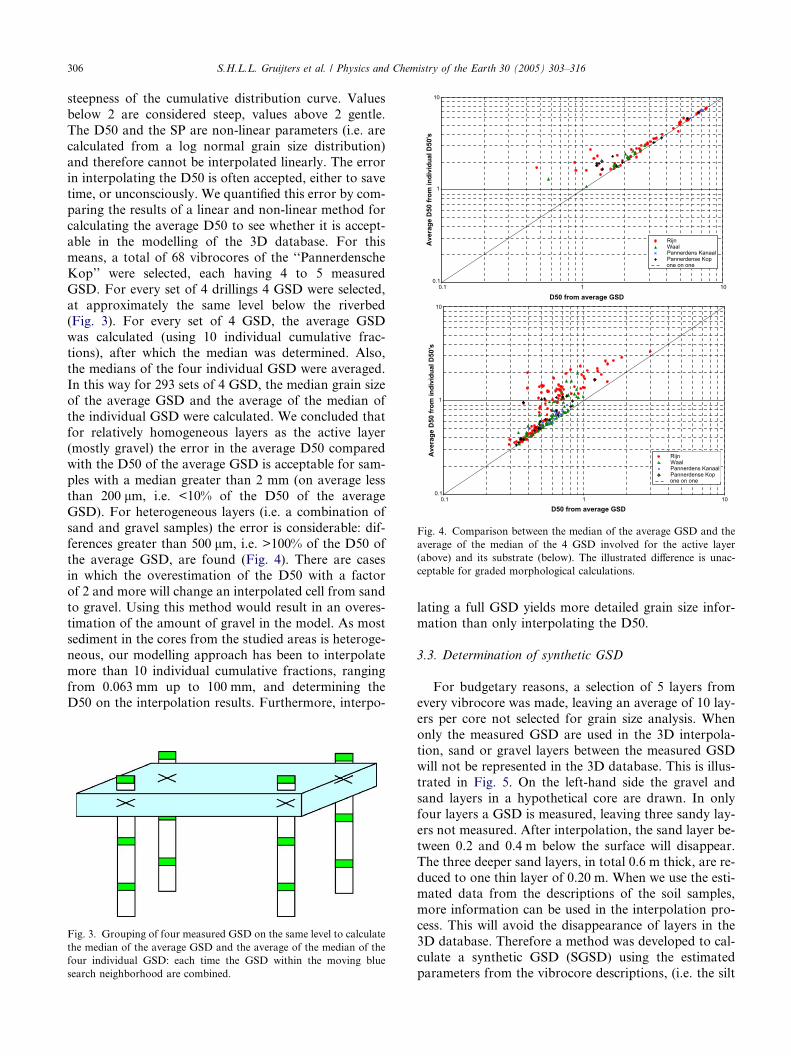
Fig. 4. Comparison between the median of the average GSD and the

average of the median of the 4 GSD involved for the active layer

(above) and its substrate (below). The illustrated difference is unac-

ceptable for graded morphological calculations.


steepness of the cumulative distribution curve. Values

below 2 are considered steep, values above 2 gentle.

The D50 and the SP are non-linear parameters (i.e. are

calculated from a log normal grain size distribution)

and therefore cannot be interpolated linearly. The error

in interpolating the D50 is often accepted, either to savetime, or unconsciously. We quantified this error by com-

paring the results of a linear and non-linear method for

calculating the average D50 to see whether it is accept-

able in the modelling of the 3D database. For this

means, a total of 68 vibrocores of the ‘‘Pannerdensche

Kop’’ were selected, each having 4 to 5 measured

GSD. For every set of 4 drillings 4 GSD were selected,

at approximately the same level below the riverbed(Fig. 3). For every set of 4 GSD, the average GSD

was calculated (using 10 individual cumulative frac-

tions), after which the median was determined. Also,

the medians of the four individual GSD were averaged.

In this way for 293 sets of 4 GSD, the median grain size

of the average GSD and the average of the median of

the individual GSD were calculated. We concluded that

for relatively homogeneous layers as the active layer(mostly gravel) the error in the average D50 compared

with the D50 of the average GSD is acceptable for sam-

ples with a median greater than 2 mm (on average less

than 200 lm, i.e. <10% of the D50 of the average

GSD). For heterogeneous layers (i.e. a combination of

sand and gravel samples) the error is considerable: dif-

ferences greater than 500 lm, i.e. >100% of the D50 of

the average GSD, are found (Fig. 4). There are casesin which the overestimation of the D50 with a factor

of 2 and more will change an interpolated cell from sand

to gravel. Using this method would result in an overes-

timation of the amount of gravel in the model. As most

sediment in the cores from the studied areas is heteroge-

neous, our modelling approach has been to interpolate

more than 10 individual cumulative fractions, ranging

from 0.063 mm up to 100 mm, and determining theD50 on the interpolation results. Furthermore, interpo-

Fig. 3. Grouping of four measured GSD on the same level to calculate

the median of the average GSD and the average of the median of the

four individual GSD: each time the GSD within the moving blue

search neighborhood are combined.

lating a full GSD yields more detailed grain size infor-mation than only interpolating the D50.

3.3. Determination of synthetic GSD

For budgetary reasons, a selection of 5 layers from

every vibrocore was made, leaving an average of 10 lay-

ers per core not selected for grain size analysis. When

only the measured GSD are used in the 3D interpola-tion, sand or gravel layers between the measured GSD

will not be represented in the 3D database. This is illus-

trated in Fig. 5. On the left-hand side the gravel and

sand layers in a hypothetical core are drawn. In only

four layers a GSD is measured, leaving three sandy lay-

ers not measured. After interpolation, the sand layer be-

tween 0.2 and 0.4 m below the surface will disappear.

The three deeper sand layers, in total 0.6 m thick, are re-duced to one thin layer of 0.20 m. When we use the esti-

mated data from the descriptions of the soil samples,

more information can be used in the interpolation pro-

cess. This will avoid the disappearance of layers in the

3D database. Therefore a method was developed to cal-

culate a synthetic GSD (SGSD) using the estimated

parameters from the vibrocore descriptions, (i.e. the silt

Dep

th

Lith

olog

y

Mea

sure

d fr

actio

n

frac

tion

> 2

mm

lith

olog

y

0.2 G 50 50 G

0.4 S 45 G

0.6 G 40 40 G

0.8 S Interpolation→ 25 S

1.0 S 10 10 S

1.2 S 35 G

1.4 G 60 60 G

S: sand, G: Gravel

Dep

th

Lith

olog

y

Mea

sure

d fr

actio

n

> 2m

m

Est

imat

ed f

ract

ion

> 2

mm

frac

tion

> 2

mm

lith

olog

y

0.2 G 50 50 G

0.4 S 20 20 S

0.6 G 40 40 G

0.8 S 20 interpolation → 20 S

1.0 S 10 10 S

1.2 S 25 25 S

1.4 G 60 60 G

2m

m

(a) (b)

>

Fig. 5. (a) Effect of a limited number of measured GSD on the lithology after interpolation: layers without a measured GSD may disappear.

(b) Effect of using measured and estimated GSD on the lithology after interpolation: every layer is represented.


content, the median grain size of the sand fraction and

the gravel content) and the grain size information from

the measured samples. This method consists of the fol-

lowing steps:

1. Select an analytical function describing the shape of a

GSD: the arctan function (ATAN).2. Transform this function so the median grain size and

the steepness of the synthetic GSD can be calculated

from 2 (estimated) grain size data points.

3. Divide the data in two sets: dataset 1 containing sam-

ples having both measured and estimated grain size

parameters, and dataset 2 having only estimated

grain size parameters. Check how well the SGSD

describes the measured GSD, using the measured siltcontent, the measured median grain size of the sand

fraction and the measured gravel content of the sam-

ples in dataset 1 as input for the SGSD. If necessary,

calculate a correction for every fraction.

4. Check the difference between the estimated and the

measured grain size parameters, again using the set

of samples from dataset 1, having both measured

and estimated grain size parameters. If necessarycalculate a correction factor for the estimated

parameters.

5. Use the estimated parameters (silt content, median

grain size of the sand fraction, gravel content and

the constant chosen maximum gravel diameter) from

the core samples of dataset 2 to calculate the SGSD,

applying the corrections from steps 3 to 4.

Ad 1: select an analytical function. We chose an

ATAN function because we needed an equation describ-

ing the shape of a cumulative grain size distribution

which could analytically be transformed in such a way

that, using the estimated grain size data points for input,

a complete GSD can be calculated. It is common to use

a Gausian cumulative density function (cdf) function to

describe a GSD curve. However the construction of a

SGSD based on (a combination of) Gaussian cdf func-

tions is much more complex and the resulting SGSD

did not describe the measured GSD more accurate.

Ad 2: construct a SGSD. The ATAN function used 2parameters to define the median grain size (‘‘a’’) and the

steepness of the curve (‘‘b’’). The formula used for the

SGSD is:

y ¼ 200 � ATAN ðx=pÞ ð1Þ

with

y cumulative sieve residue [%] scale 1–100%

x (sieve diameter)/a^b

a parameter determining the median grain size of

the SGSD [mm]

b parameter determining the steepness of the

SGSD [-]. b = 3: steep, b = 1: gentle

Making the factor ‘‘a’’ and ‘‘b’’ explicit results in (seeFig. 6 for an example):

a¼ sieve 1

10^ 1

b� log TAN

ðcum fraction 1� 100Þ � p�200

� ��

ð2Þ

b ¼

log

TANðcum fraction 2 � 100Þ � p

�200

� �

TANðcum fraction 1 � 100Þ � p

�200

� �0BB@

1CCA

logsieve 2

sieve 1

� � ð3Þ

0

20

40

60

80

100

0.01 0.1 10 100

sieve [mm]

< si

eve

[m/m

%]

0

20

40

60

80

100

> si

eve

[m/m

%]

sieve_1: 0.1 mmcum_fraction_1: 80 %m/m

sieve_2: 5 mmcum_fraction_2: 10 %m/m

parameters forATAN function:a = 0.44 mmb = 0.758

1

Fig. 6. Example of an ATAN fit (Eq. (1)) based on 2 data points. The

first point: 80 m/m% on sieve 0.1 mm, the second point: 10 m/m% on

sieve 5 mm. The corresponding parameters for the ATAN fit are:

a = 0.44 mm (Eq. (2)), b = 0.758 (Eq. (3)).


with

sieve_1 diameter of first estimated point [mm]sieve_2 diameter of second estimated point [mm]

cum_fraction_1 cumulative fraction > sieve of first

(estimated) point [m/m%]

cum_fraction_2 cumulative fraction > sieve of second

(estimated) point [m/m%]

The final SGSD was calculated by the combination of

three ATAN functions, so non-symmetrical GSD can becalculated (see Fig. 7 for an example):

• First ATAN: Between the (estimated) silt content and

the (estimated) median grain size of the sand fraction.

• Second ATAN: Between the (estimated) median

grain size of the sand fraction and the (estimated)

gravel content.

0

10

20

30

40

50

60

70

80

90

1000.01 0.1

sieve

> si

eve

[m/m

%]

1st ATAN

2nd ATAN

3rd ATAN

1

Fig. 7. Example of a SGSD constructed of three ATAN fits (Eq. (1)): the first

fraction, the second part on the median grain size of the sand fraction and th

>63 mm (set at a constant value of 0.05%).

• Third ATAN: Between the (estimated) gravel content

and the maximum gravel diameter of the sediments

involved. For this study this point was set at 0.05%

greater than 63 mm.

Ad 3: correct for the shape of the SGSD using dataset 1.We used the 621 measured GSD from the ‘‘IJssel Kop’’

(dataset 1) to check how good the SGSD describes the

shape of the measured GSD. For each GSD we calcu-

lated a SGSD using the measured grain size parameters

(silt content, median grain size of the sand fraction and

gravel content) as input (Fig. 8, left). It is clear that the

fit is not very accurate, showing a mismatch at the fine

and coarser end of the distributions. Therefore theATAN function was corrected for each fraction to

accommodate the less symmetric shape of the measured

GSD (Fig. 8, right). This correction was calculated for

every sieve by a spline fitting through the difference in

measured and synthetic cumulative fractions for the

621 samples.

Ad 4: correct for the difference between estimated and

measured grain size parameters using dataset 1. The esti-mated grain size parameters (silt content, median grain

size of the sand fraction and gravel content) differ sys-

tematically from the measured ones. Again the subset

of 621 GSD (dataset 1) was used to calculate the differ-

ence between the estimated and measured grain size

parameters. For the median grain size and the gravel

content a spline fitting through these differences was

calculated.Ad 5: calculate a SGSD for samples only having esti-

mated grain size parameters (dataset 2). Finally, for

the 1171 samples only having estimated grain size

parameters (dataset 2) a SGSD was calculated, applying

the corrections for the error in the estimated grain size

parameters and the shape of the SGSD.

10 100 [mm]

measured

SGSD

based on the fraction >0.063 lm and the median grain size of the sand

e gravel content, the third part on the gravel content and the fraction

0

10

20

30

40

50

60

70

80

90

100

Sieve [mm]

0

10

20

30

40

50

60

70

80

90

100

GRAVELSANDSILTCLAY zgmgfugzgmgmfzfuf

Gravel, measured

0

10

20

30

40

50

60

70

80

90

100

Sieve [mm]

0

10

20

30

40

50

60

70

80

90

100

GRAVELSANDSILTCLAY zgmgfugzgmgmfzfuf

Sand, measured

0

10

20

30

40

50

60

70

80

90

100

Sieve [mm]

0.00

10.00

20.00

30.00

40.00

50.00

60.00

70.00

80.00

90.00

100.00

GRAVELSANDSILTCLAY

zgmgfugzgmgmfzfuf

Sand, measured

0

10

20

30

40

50

60

70

80

90

100

0.001 0.01 0.1 1 10 100

0.001 0.01 0.1 1 10 100

0.001 0.01 0.1 1 10 100

0.001 0.01 0.1 1 10 100

Sieve [mm]

0.00

10.00

20.00

30.00

40.00

50.00

60.00

70.00

80.00

90.00

100.00

GRAVELZANDSILTKLEI

zgmgfugzgmgmfzfuf

Gravel,measured

> s

ieve

[m/m

%]

> s

ieve

[m/m

%]

> si

eve

[m/m

%]

> s

ieve

[m/m

%]

< s

ieve

[m/m

%]

< si

eve

[m/m

%]

< s

ieve

[m/m

%]

< s

ieve

[m/m

%]

Fig. 8. Results of the fitting of the parameters a and b in the used ATAN function for the synthetic GSD for the 621 measured GSD before (left) and

after (right) the empirical correction. The black solid lines represent the 90% reliability interval, the dashed line the median of the synthetic GSD. The

colored figures represent the 90% reliability interval of the measured GSD (yellow for the sand samples, red for the gravel samples).


3.4. 3D interpolation

We have used a 3D kriging routine for the interpola-

tions (Deutsch and Journel, 1998). Kriging uses vario-

grams to weigh the different samples and calculate an

estimated value at a grid point. The shape of the vario-gram, the value of the relative nugget (relative to the

total semi variance) and the search neighborhood deter-

mine the amount of smoothing of the data (Isaaks and

Srivastava, 1989). For both bifurcations, the spatial cor-

Fig. 9. Example of the combination of the measured seismic data and vibroc

clay/peat layer (solid black line).

relation was examined calculating different variograms

for each fraction per layer in the geological model and

for different directions (i.e. parallel and perpendicular

to the flow direction of the river).

At the ‘‘Pannerdensche Kop’’ the sampling scheme

appeared to be unsuitable to detect the spatial variationin grain size distributions on a scale of 10–200 m. Typi-

cal values for the relative nugget for the coarser frac-

tions in the deeper layers (>1 mm) were 0.2 up to 0.5

with ranges between 500 and 750 m. For the active layer

ores, showing both the active layer (dashed black line) and the top of a

https://www.researchgate.net/publication/223272644_Stochastic_modelling_of_a_fluvial_reservoir_A_comparative_review_of_algorithms?el=1_x_8&enrichId=rgreq-7080326e-2b4f-412b-bd33-7ea22b94785b&enrichSource=Y292ZXJQYWdlOzI0ODU1MDA1OTtBUzoyNjEyNDY5MzA5MTEyMzNAMTQzOTI5NzUzMDU0NQ==


a relative nugget of 0.4 to 0.6 with ranges between 1400

and 2100 m were found. We used a search neighborhood

with a radius up to two times the ranges in the vario-

grams, allowing more distant data points to assist in

the estimation of the local mean (Deutsch and Journel,

1998), (Isaaks and Srivastava, 1989). For the ‘‘IJsselKop’’ an adapted sampling scheme was used (see Fig.

1). In addition at three locations in the centre line, five

vibrocores were placed at 10, 25 50, 100 and 200 m dis-

tance. This allowed detection of both short range

(<400 m) and long range (400–2000 m) spatial correla-

tion. The data showed a relative nugget of 0.1 and a

range of 1725 m for the coarse fractions (>1 mm) in

the active layer. The fine fractions (<1 mm) showed arelative nugget of 0.25 and a range of 225 m. For the

substrate, a relative nugget of 0.1 was found, with a

range of 200 m. In the interpolation, both the short

and the long range spatial correlation were combined

in a stacked variogram function.

3.5. Comparing the interpolation results with

measurements

The variation in the datasets was described by an

envelope capturing 90% of all measured grain size distri-

butions. This envelope is determined by calculating the

interval containing 90% of the measured data points

Fig. 10. Typical difference between the active layer (often containing Carbic

90% of all measured grain size distributions in the active layers (top) and its su

Also the results of the vibrocore drilling 40B0503 is shown (right), where the

(rest).

for each fraction. This is done for both the measured

GSD as the interpolation results. By comparing both

envelopes the representation of the spatial variation in

GSD was evaluated: the better the fit, the better the spa-

tial variation is represented, with less smoothing of the

data. As the median grain size (D50) and the spreadparameter (SP) are the most important parameters used

as input for morphological calculations, these parame-

ters are chosen for comparing the interpolation results

with the measurements. The cumulative probability den-

sity of these two parameters was calculated for both

measured as interpolated GSD within the active layer

and its substrate for the entire model. To illustrate the

spatial distribution of the interpolation results in themodel, the fraction greater then 2 mm is plotted at a

cross section of the model at the centre of the river, near

the bifurcation, showing both the measurements as the

interpolated values.

4. Results

4.1. Interpretation of the seismic recordings

The active layer is clearly visible in seismic recordings

(Fig. 9). In vibrocore samples it was recognized by traces

of (sub)recent anthropogenic debris and Corbicula flumi-

ula fulminea) and its substrate illustrated with the envelope capturing

bstrate (bottom) at the Pannerdensch Kanaal in the IJssel Kop project.

active layer (top 75 cm) can be clearly distinguished from its substrate


nea valves, an Asian/African exotic mollusc which colo-

nized European river areas since 1980 and was first dis-

covered in the Rhine about a decade ago. Also, the

relative low content of sand in the samples was consid-

ered diagnostic for the active layer. The measured

GSD show the typical difference between the active layerand the substrate: coarser, gravely samples in the active

layer and finer, sandy samples in the substrate. Also the

variation in grain size in the active layer is smaller than

in its substrate (Fig. 10). In the substrate peat, clay and

other clastic units have been clearly recognized in seis-

mic recordings (Fig. 9). Gravel-sand transitions in the

0

10

20

30

40

50

60

70

80

90

1000.001 0.01 0.1

0.001 0.01 0.1

SANSILTCLAY

zmgmfzfuf

0

10

20

30

40

50

60

70

80

90

100

SANSILTCLAY

zmgmfzfuf

Sieve

Sieve

> s

ieve

[m/m

%]

> s

ieve

[m/m

%]

Fig. 11. Results of the interpolation for the ‘‘Pannerdensche Kop’’ data for th

symbols denote the 5% upper and 5% lower reliability threshold per fraction,

The gray area in the top graph represents the envelope capturing 90% of all o

that of its substrate. Note the smoothing of the measured data (i.e. a sma

neighborhood (�1–1.5 times the range), especially in the substrate.

substrate turned out to be undetectable in the seismic

recordings.

4.2. Interpolation results

The results of the interpolation for the ‘‘Pannerden-sche Kop’’ bifurcation (not using SGSD) are shown in

Figs. 11 and 12. The interpolation method smoothed

the actual variation in GSD considerably, due to the

rather large search neighborhood and the large value

of the relative nugget. It is clear that for the substrate

this smoothing is even larger, due to the greater

1 10 100

1 10 100

GRAVELDzgmgfugg

GRAVELDzgmgfugg

[mm]

[mm]

e active layer (above) and its substrate (below). The solid lines with the

the solid dashed line represents the median of the interpolation results.

f the measured data in the active layer, the gray area in the lower graph

ller envelope) due to the Kriging interpolation using a large search

0

0.1

0.2

0.3

0.4

0.5

0.6

0.7

0.8

0.9

1

0 2 4 6 8 10 12 14

D50 [mm]

prob

abili

ty

interpolated data

measured data

interpolation too fine

0

0.1

0.2

0.3

0.4

0.5

0.6

0.7

0.8

0 2 4 6 8 10 12 14

prob

abili

ty

interpolated data

measured data

0

0.1

0.2

0.3

0.4

0.5

0.6

0.7

0.8

0 1 2 3 4 5 6 7 8 9 10

prob

abili

ty

interpolated data

measured data

0

0.1

0.2

0.3

0.4

0.5

0.6

0.7

0.8

0.9

1

0 1 2 3 4 5 6 7 8 9

SP=0.5*(D84/D50+D50/D16) [-]

D50 [mm] SP=0.5*(D84/D50+D50/D16) [-]

prob

abili

ty

interpolated data

measured data

0.9

1

0.9

1


Fig. 12. Results of the interpolation for the ‘‘Pannerdensche Kop’’ data for the active layer (above) and its substrate (below). The cumulative

probability density function of the D50 (left) and the SP (right) are shown. The mismatch is evident: the interpolation results contain GSD which are

to fine and the variation in the SP is to small (indicating more averaging due to the interpolation), again especially in the substrate. Note that the

active layer is far more homogeneous than its substrate.

0 10 20 30 40 50 60 70 80 90 100 0 100 250 m

-2 -2

-1 -1

0 0

1 1

2 2

3 3

4 4

40D

0165

40D

0168

40G

0114

40G

0119

40G

0127

EC

EC

EC

EC

EC

EC

EC

EC

EC

EC

EC

ECEC

EC

EC

EC

EC

EC

ECEC

EC

EC

EC

EC

EC

EC

EC

ECEC

ECEC

EC

EC

EC

BX

EC

EC

EC

EC

EC

EC

EC

EC

EC

EC

67

38

78

27

13

11

82

79

63

58

50

39

4

15

677072517040

4

Fig. 13. Cross section through the model of the ‘‘Pannerdensche Kop’’ of the fraction greater than 2 mm. The section contains rather large areas with

little difference in the calculated gravel content, illustrating the underestimation of the spatial variation in the subsoil.


0

10

20

30

40

50

60

70

80

90

100

0.001 0.01 0.1 1 10 100

0.001 0.01 0.1 1 10 100

0

10

20

30

40

50

60

70

80

90

100

GRAVELSANDSILTCLAYzgmgfugzgmgmfzfuf

0

10

20

30

40

50

60

70

80

90

100 0

10

20

30

40

50

60

70

80

90

100

GRAVELSANDSILTCLAY

zgmgfugzgmgmfzfuf

Sieve [mm]

Sieve [mm]

> s

ieve

[m/m

%]

> si

eve

[m/m

%]

< s

ieve

[m/m

%]

< s

ieve

[m/m

%]

Fig. 14. Results of the interpolation for the ‘‘IJssel Kop’’ data for the active layer (above) and its substrate (below). The solid lines with the symbols

denote the 5% upper and 5% lower reliability threshold per fraction, the solid dashed line represents the median of the interpolation results. The gray

area in the top graph represents the envelope capturing 90% of all of the measured data in the active layer, the gray area in the lower graph that of its

substrate. Note the better reproduction of the measured data due to the adapted Kriging interpolation and the use of synthetic GSD.


variation in the measured data (Fig. 11). The interpola-

tion results in a model containing GSD which are toofine. The variation in the SP is clearly too small, indicat-

ing significant averaging due to the interpolation (Fig.

12). The comparison of measured and interpolated val-

ues of the sediment fraction greater than 2 mm (C2) is

shown in Fig. 13. This shows rather large areas with

comparable interpolated values, underestimating the

spatial variation in the measured GSD.

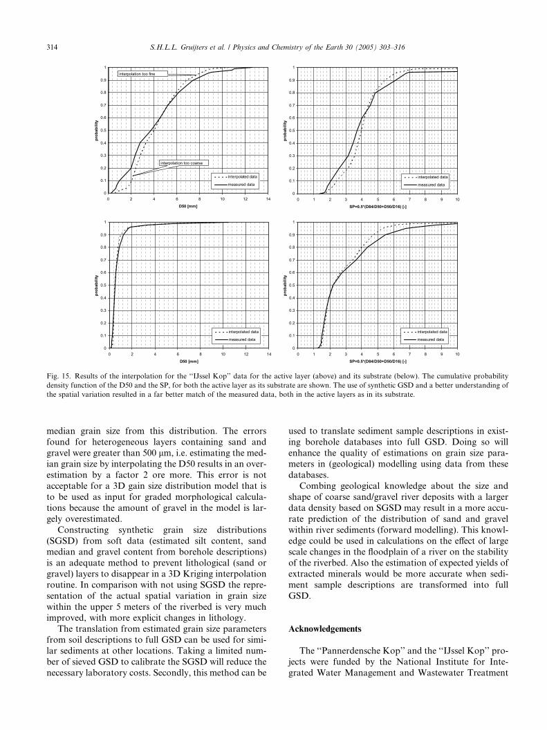
The results for the ‘‘IJssel Kop’’ bifurcation areshown in Figs. 14 and 15. The envelope capturing 90%

of all the interpolated GSD almost perfectly fits the

envelope of the measured GSD, for both the active layer

and its substrate (Fig. 14). Also the D50 and the SF are

very well reproduced (Fig. 15). The better representationof the spatial variation of the measured GSD using the

SGSD is illustrated in Fig. 16. Clearly more realistic var-

iation in gravel content exists in the model, showing

more individual pockets of gravel or sand.

5. Conclusions

This article quantifies the error resulting from inter-

polating the median grain size instead of interpolating

the entire grain size distribution and calculating the

0

0.1

0.2

0.3

0.4

0.5

0.6

0.7

0.8

0.9

1

0 2 4 6 8 10 12 14

D50 [mm]

prob

abili

ty

interpolated data

measured data

0

0.1

0.2

0.3

0.4

0.5

0.6

0.7

0.8

0.9

1

0 1 2 3 4 5 6 7 8 9 10

SP=0.5*(D84/D50+D50/D16) [-]

prob

abili

ty

interpolated data

measured data

0

0.1

0.2

0.3

0.4

0.5

0.6

0.7

0.8

0.9

1

0 1 2 3 4 5 6 7 8 9 10

SP=0.5*(D84/D50+D50/D16) [-]

prob

abili

ty

interpolated data

measured data

0

0.1

0.2

0.3

0.4

0.5

0.6

0.7

0.8

0.9

1

0 2 4 6 8 10 12 14

D50 [mm]

prob

abili

ty

interpolated data

measured data


interpolation too coarse

Fig. 15. Results of the interpolation for the ‘‘IJssel Kop’’ data for the active layer (above) and its substrate (below). The cumulative probability

density function of the D50 and the SP, for both the active layer as its substrate are shown. The use of synthetic GSD and a better understanding of

the spatial variation resulted in a far better match of the measured data, both in the active layers as in its substrate.


median grain size from this distribution. The errors

found for heterogeneous layers containing sand and

gravel were greater than 500 lm, i.e. estimating the med-ian grain size by interpolating the D50 results in an over-

estimation by a factor 2 ore more. This error is not

acceptable for a 3D gain size distribution model that is

to be used as input for graded morphological calcula-

tions because the amount of gravel in the model is lar-

gely overestimated.

Constructing synthetic grain size distributions

(SGSD) from soft data (estimated silt content, sandmedian and gravel content from borehole descriptions)

is an adequate method to prevent lithological (sand or

gravel) layers to disappear in a 3D Kriging interpolation

routine. In comparison with not using SGSD the repre-

sentation of the actual spatial variation in grain size

within the upper 5 meters of the riverbed is very much

improved, with more explicit changes in lithology.

The translation from estimated grain size parametersfrom soil descriptions to full GSD can be used for simi-

lar sediments at other locations. Taking a limited num-

ber of sieved GSD to calibrate the SGSD will reduce the

necessary laboratory costs. Secondly, this method can be

used to translate sediment sample descriptions in exist-

ing borehole databases into full GSD. Doing so will

enhance the quality of estimations on grain size para-meters in (geological) modelling using data from these

databases.

Combing geological knowledge about the size and

shape of coarse sand/gravel river deposits with a larger

data density based on SGSD may result in a more accu-

rate prediction of the distribution of sand and gravel

within river sediments (forward modelling). This knowl-

edge could be used in calculations on the effect of largescale changes in the floodplain of a river on the stability

of the riverbed. Also the estimation of expected yields of

extracted minerals would be more accurate when sedi-

ment sample descriptions are transformed into full

GSD.

Acknowledgements

The ‘‘Pannerdensche Kop’’ and the ‘‘IJssel Kop’’ pro-

jects were funded by the National Institute for Inte-

grated Water Management and Wastewater Treatment

Fig. 16. Results of the 3D interpolation of the fraction >2 mm, without (above) and with (below) synthetic GSD for the ‘‘IJssel Kop’’ dataset. Using

the synthetic GSD clearly results in a more differentiated model with more explicit changes in lithology.


(RIZA). We would like to thank P. Jesse and L.J. Bol-widt (RIZA) for giving the permission to use the results

of these studies for this paper. Furthermore, we thank

J. Gunnink, M.P.E. de Kleine, M.J. van der Meulen

and H.J.T. Weerts (TNO) for their advice and stimulat-

ing comment, both during the execution of the projects

involved and in the writing process of this paper.

References

Anthony, D., Moller, I., 2002. The geological architecture and

development of the Holmsland Barrier and Ringkobing Fjord

area, Danish North Sea Coast. Danisch Journal of Geography 101,

26–36.

Asselman, N.A.M., 1999. Grain-size trends used to assess the

effective discharge for floodplain sedimentation, river Waal the


Netherlands. Netherlands Journal of Sedimentary Research 69, 51–

61.

Bosch, J.H.A., 2000. Standaard boorbeschrijf methode, versie 5.1,

rapport NITG 00-141-A, TNO-NITG, Zwolle, The Netherlands.

Blom, A., 2003. A vertical sorting model for rivers with non-uniform

sediment and dunes. Ph.D. thesis, University of Twente, Enschede,

The Netherlands.

Blom, A., Parker, G., 2004. Vertical sorting and morphodynamics of

bed form dominated rivers: A modeling framework. Journal of

Geophysical Research 109, F02007.

Deutsch, C.V., Journel, A.G, 1998. GSLIB, Geostatistical

Software Library and Users Guide. Oxford University Press,

Oxford.

Eggleston, J.R., Rojstaczer, S.A., Peirce, J.J., 1996. Identification of

hydraulic conductivity structure in sand and gravel aquifers: Cape

Cod data set. Water Resources Research 32, 1209–1222.

Fogg, G.E., Noyes, C.D., Carle, S.F., 1998. Geologically based model

of heterogeneous hydraulic conductivity in an alluvial setting.

Hydrogeology Journal 6, 131–143.

Gruijters, S.H.L.L., Gunnink, J., Hettelaar, H., de Kleine, M.,

Maljers, D.,Veldkamp, J., 2003. Kartering ondergrond IJssel

Kop, Fase 3, eindrapport, Internal report NITG 03-120-B, TNO-

NITG, Utrecht, The Netherlands.

Gruijters, S.H.L.L., Gunnink, J., Veldkamp, J., Bosch, J.H.A., 2001.

De lithologische en sedimentologische opbouw van de ondergrond

van de Pannerdensche Kop, Internal report NITG 01-166-B, TNO-

NITG, Utrecht, The Netherlands.

Isaaks, E.H., Srivastava, R.M., 1989. An Introduction to Applied

Geostatistics. Oxford University Press, Oxford.

Journel, A.G., Gundeso, R., Gringarten, E., Yao, T., 1998. Stochastic

modeling of a fluvial reservoir: A comparative review of algo-

rithms. Journal of Petroleum Science and Engineering 21, 95–121.

Koltermann, C.E., Gorelick, S.M., 1996. Heterogeneity in sedimentary

deposits: A review of structure-imitating, process-imitating, and

descriptive approaches. Water Resources Research 32, 2617–2658.

NEN, 2000. NEN 2560, Test sieves—Wirescreens, Perforated plates

and electroformed sheets with round and square holes.

RAW, 1995. RAW standard conditions of contract for works of civil

engineering construction. CROW, Ede, pp. 54–55 and 68–72.

Rice, S., 1999. The nature and controls on downstream fining within

sedimentary links. Journal of Sedimentary Research 69, 32–39.

Rice, S., Church, M., 1998. Grain size along two gravel-bed rivers:

Statistical variation, spatial pattern and sedimentary links. Earth

Surface Processes and Landforms 23, 345–363.

Simpkin, P.G., 1996. High resolution seismic profiling in three river

systems. In: Proceedings of 2nd Meeting, Environmental and

Engineering Geophysical Society, European Section. Nantes,

France.

Sloff, C.J., Bernabe, M., Baur, T., 2003. On the stability of the

Pannerdensche Kop river bifurcation. In: Proceedings River,

Coastal and Estuarine Morphodynamics. pp. 1001–1011.

Toth, T., Simpkin, P.G., Vida, R., Horvath, F., 1997. Shallow water

single and multichannel seismic profiling in a riverine environment.

Society of Exploration Geophysicists—The Leading Edge 16,

1691–1695.

Wang, L., Wong, P.M., Shibli, S.A.R., 1998. A review of geostatistical

simulation algorithms for lithofacies architecture and modelling.

Appea Journal, 889–890.

3D interpolation of grain size distributions in the upper 5m of the channel bed of three lower Rhine...

Documents

Transcript of 3D interpolation of grain size distributions in the upper 5m of the channel bed of three lower Rhine...