From grain size to tectonics

R. A. Duller,1 A. C. Whittaker,1 J. J. Fedele,2 A. L. Whitchurch,1 J. Springett,3

R. Smithells,4 S. Fordyce,5 and P. A. Allen1

Received 13 August 2009; revised 21 December 2009; accepted 30 March 2010; published 14 August 2010.

[1] Regional grain size trends in fluvial successions can reveal important informationregarding the dynamics of sediment routing systems. Self‐similar solutions for down‐system grain size fining have recently been proposed to explore how key variables, suchas the spatial distribution of deposition, sediment discharge, and sediment supplycharacteristics, control spatial distribution of grain size in fluvial successions over timescales of 104–106 years. We explore the sensitivity of these solutions to changes in keyvariables and assess their applicability to ancient fluvial successions. Several sensitivityanalyses are presented to investigate the relative control of the key model variables on thespatial pattern of down‐system grain size fining in fluvial successions. Sensitivityanalyses demonstrate that (1) an increase in the initial value of sediment discharge to a basincauses a decrease in the rate of grain size fining in fluvial successions, an effect thatbecomes nonlinear for large values of initial sediment discharge; (2) a short‐wavelength/high‐amplitude subsidence regime generates a greater rate of down‐system grain sizefining and a long‐wavelength/lower‐amplitude subsidence regime generates a lesser rateof down‐system grain size fining in fluvial successions; and (3) an increase in the spread ofgrain sizes in the sediment supply generates a greater rate of down‐system grain sizefining. We apply this modeling technique to grain size data sets collected from two timesurfaces within conglomerates of the Upper Eocene Montsor Fan Succession of the PoblaBasin, Spanish Pyrenees. These data sets exhibit approximately self‐similar grain sizedistributions; further, the observed increase in down‐system grain size fining associated withsmaller depositional system lengths provides support for the application of self‐similarsolutions to fluvial successions. By applying these solutions to carefully collected grain sizedata from fluvial successions, we are able to relate explicitly the initial grain size suppliedto the system, the spatial distribution of subsidence and the sediment discharge intothe basin to the rate of grain size fining in fluvial successions. This method thus offers apowerful means of elucidating sediment routing system dynamics over time.

Citation: Duller, R. A., A. C. Whittaker, J. J. Fedele, A. L. Whitchurch, J. Springett, R. Smithells, S. Fordyce, and P. A. Allen(2010), From grain size to tectonics, J. Geophys. Res., 115, F03022, doi:10.1029/2009JF001495.

1. Introduction

1.1. Motivation

[2] In nonglaciated terrain, fluvial systems are the primarymechanism bywhich sediment is eroded and transported fromupland areas to depositional basins. Because fluvial systemsare sensitive to long‐term changes in boundary conditions, it

can be inferred that the sedimentary record represents a time‐integrated archive of the erosional‐depositional response offluvial systems to both tectonic and climatic boundary con-ditions [Heller and Paola, 1992;Whipple, 2004;Allen, 2008].It is therefore implied that if sedimentary deposits are formedas a result of these boundary conditions, it could, in principle,be possible to decode tectonic and/or climatic signals fromtime‐integrated geomorphological and stratigraphical inves-tigations [Hovius and Leeder, 1998; Allen and Hovius, 1998;Robinson and Slingerland, 1998; Leeder et al., 1998; Weltjeet al., 1998; Allen and Densmore, 2000; Sheets et al., 2002;Densmore et al., 2007]. The temporal and spatial patterns ofsediment accumulation and the characteristics of materialextracted to form fluvial successions are a function of theinterplay between tectonic subsidence and sediment dis-charge [Paola and Seal, 1995; Strong et al., 2005]. Onecharacteristic indicator of this interplay is the spatial distri-bution of grain size within sedimentary basins [Paola et al.,

1Department of Earth Sciences and Engineering, Imperial College,London, UK.

2Department of Earth and Atmospheric Sciences, St. Cloud StateUniversity, St. Cloud, Minnesota, USA.

3ExxonMobil International Limited, Leatherhead, Surrey, UK.4School of Physical and Geographical Sciences, Keele University,

Staffordshire, UK.5Novas Consulting Ltd., Abbey House, Slough, Berkshire, UK.

Copyright 2010 by the American Geophysical Union.0148‐0227/10/2009JF001495

JOURNAL OF GEOPHYSICAL RESEARCH, VOL. 115, F03022, doi:10.1029/2009JF001495, 2010

F03022 1 of 19

1992a; Heller and Paola, 1992; Robinson and Slingerland,1998; Marr et al., 2000]. Temporal and spatial trends insediment caliber of fluvial successions, together with themigration of specific grain size discontinuities, containimportant information about the time‐integrated behaviorof sediment routing systems and their sensitivity to externalforcing mechanisms. A crucial hurdle to overcome indecoding grain size trends in fluvial successions is therequirement for knowledge that cannot be measured orinferred from fluvial successions, such as knowledge of thedetailed mechanism(s) that contribute to the transfer of sedi-ment grains at the Earth’s surface to the geological record[cf. Paola et al., 2001; Strong et al., 2005; Allen, 2008].

1.2. Background

[3] Down‐system grain size fining in fluvial systems isdriven primarily by the selective transport and deposition ofparticles and secondarily by abrasion of the particles duringtransport [Parker, 1991; Paola et al., 1992b; Hoey and Bluck,1999]. Numerous studies have investigated and quantitativelyassessed down‐system grain size variation in modern fluvialsystems [Sternberg, 1875; Paola and Wilcock, 1992; Paolaet al., 1992b; Van Niekerk et al., 1992; Sambrook‐Smith andFerguson, 1995; Seal and Paola, 1995; Paola and Seal,1995; Ferguson et al., 1996; Hoey and Ferguson, 1997;Dade and Friend, 1998; Hoey and Bluck, 1999; Rice, 1999,2005; Wilcock and Kenworthy, 2002] and in ancient fluvialsuccessions [e.g., Flemings and Jordan, 1989; Paola et al.,1992a; Rivenæs, 1992; Marr et al., 2000; Simpson andSchlunegger, 2003], the latter demonstrating that basin‐wide stratigraphic architectures and major grain size dis-continuities can be captured dynamically via diffusional massbalance. The advantage of a diffusional approach is that itsimplifies or averages the long‐term dynamics and behaviorof fluvial systems and in doing so provides approximateestimates of the temporal and spatial evolution of grainsize fronts in fluvial successions [cf. Marr et al., 2000;Paola, 2000].[4] In contrast to the diffusional approach, Robinson and

Slingerland [1998] couple a physically based grain sizesorting model [Van Niekerk et al., 1992] to fluvial aggra-dation in a foreland basin. The model of Robinson andSlingerland [1998] differs from that of diffusional modelsas, under a prescribed spatial distribution of tectonic sub-sidence and input grain size supply, it explores the influenceof tectonic subsidence rate, sediment discharge, water dis-charge, hydraulic geometry, and the mechanics of sedimenttransport on the spatial distribution of grain size in ancientfluvial systems. Each parameter can be varied independently,and hence, outputs (e.g., hydraulic geometry, subsidencerate, grain size) can be tested rigorously against field data[cf. Paola, 2000]. However, the general model results ofRobinson and Slingerland [1998] agree with diffusionalinvestigations of gravel progradation in fluvial successions[Paola, 1988; Heller and Paola, 1989, 1992; Paola et al.,1992a].[5] These studies show that the rate of grain size fining in

fluvial successions is governed by (1) the probability densityfunction of the input grain size supply to the system, (2) themagnitude of sediment discharge to the basin, (3) the spatialdistribution of subsidence, which controls the space availablefor sediment accumulation, and (4) the detailed mechanics

of sediment transport and deposition [Paola et al., 1992a;Paola and Seal, 1995; Robinson and Slingerland, 1998].Both the diffusional approach and the approach of Robinsonand Slingerland [1998], although powerful in their appli-cation, require knowledge of (4) to predict or interpret grainsize trends in fluvial successions. Unfortunately, a fullreconstruction of sediment transport capacity through timerequires knowledge of the time‐dependent distribution ofchannel discharges and hydraulic geometries, something thatis difficult to quantify accurately from fluvial successions.Fedele and Paola [2007] address this by developing self‐similar solutions for down‐system grain size fining, enablingworkers to investigate the controls of grain size trends influvial successions in terms of long‐term sediment dischargeand subsidence rate, parameters that are more readily attain-able from stratigraphic field studies. These solutions havebeen tested and validated over short time scales by field andlaboratory experiments but have not yet been applied to fluvialsuccessions over time scales of 104–106 years. In this paper,we first conduct a sensitivity analysis to evaluate the com-peting effects of these two variables (sediment discharge,subsidence) on grain size fining within stratigraphy. Wethen compare the output of these similarity solutions to fieldmeasurements of sediment caliber collected from the EoceneMontsor Fan Succession, Pobla Basin, Spanish Pyrenees[Mellere, 1993], where key controlling variables are wellconstrained. Specifically, this contribution aims to assessthe application of self‐similar grain size solutions to ancientfluvial successions and explore their potential usage inquantifying and predicting key controlling variables using asmall sediment routing system as a case study. If validated, thedown‐system fining model would provide a significant steptoward an understanding of ancient sediment routing systemdynamics and, inversely, to the prediction of regional grain sizetrends in fluvial successions if key controlling variables areknown.

2. Modeling Procedure

[6] In this section, we describe our model formulation forthe investigation of grain size trends in fluvial successions byincorporating the similarity solutions of Fedele and Paola[2007]. We then outline the major assumptions and require-ments of the modeling approach.

2.1. Approach

[7] A summary of grain size self‐similarity and the modelderivation is presented in Appendix A of this paper; for adetailed analysis of self‐similar solutions for down‐systemgrain size fining, the reader is referred to Fedele and Paola[2007]. The starting point of the model is the Exner sedi-ment mass balance for the long term, given as,

ð1� �pÞ ��tðxÞ þ @�

@tðxÞ

� �¼ � @qs

@x; ð1Þ

where lp is sediment porosity, sdt (x) is spatial distributionof tectonic subsidence (L t−1) over a time interval dt, ∂h/∂t(x)is rate of change of bed elevation (L t−1) at a given down‐system location, and ∂qs/∂x is down‐system change insediment discharge. The interval dt is chosen to be long

DULLER ET AL.: FROM GRAIN SIZE TO TECTONICS F03022F03022

2 of 19

enough to average out intrinsic, flow‐controlled (autogenic)fluctuations and high‐frequency variability in catchment‐related qs behavior, but short compared with the time scalesof change in tectonic boundary conditions that impact thelarge‐scale stratigraphic architecture and grain size trends[Paola et al., 1992a; Sheets et al., 2002; Strong et al., 2005].As we are modeling grain size trends in fluvial successionsover geological time scales, the rate of change of bed ele-vation over time, which is largely a function of short‐termchannel forming processes, is taken to be zero, i.e., ∂h/∂t = 0in equation (1). In other words, the overriding control on thelong‐term rate of deposition in sedimentary basins is tectonicsubsidence, so we assume that the gross rate of depositionequals the rate of tectonic subsidence [cf. Paola et al., 1992a].[8] For simplicity, we use an exponential decay function to

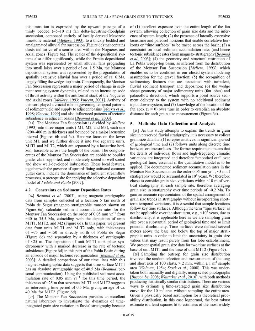
describe the spatial distribution of tectonic subsidence in ourmodel (Figure 1) as, in the absence of an explicit solution, thisapproximates the spatial distribution of subsidence in awedge‐top basin of the kind investigated in this study. Otherspatial distributions of tectonic subsidence are possible,depending on the underlying basin mechanics [Allen andAllen, 2005], but with this assumption, we have

��tðxÞ ¼ ��tðx0Þe��sx; ð2Þ

where x0 represents the position of the beginning of thedepositional segment of the fluvial system, and as para-meterizes the down‐system decay of the subsidence rate.[9] An estimate for value of the time‐averaged initial

sediment discharge qso could be made from field observationsof the spatial thickness of sedimentary units filling the basinor calculated from transport equations [e.g., Tucker andSlingerland, 1996; Paola and Swenson, 1998]. However, ifwe make the assumption that the basin is closed and is filledat the rate that accommodation is generated, i.e., all sediment

supplied to the basin is retained by the basin, then qso (qs atx = 0) is always known, being the sum of the spacemade available for sediment accumulation during the timeinterval dt,

qso ¼ZL0

��t xð Þdx: ð3Þ

As we assume instantaneous basin fill within a closed system(Figure 1), our model is purely geometric and therefore onlycaptures the effects of subsidence, not the time‐dependentdynamic response of a fluvial system to climatic and tectonicperturbations [Paola, 2000;Whittaker et al., 2007]. With thisassumption, the rate of decay of sediment discharge down‐system is described by

qs xð Þ ¼ qso � 1� �p

� � ZL

0

��t xð Þdx; ð4Þ

where L is the depositional length scale of the system.[10] From the above, we are able to calculate the spatial

distribution of sediment mass down‐system R* (Appendix A,equation (A3)) and hence the dimensionless distance trans-formation y*(x*) (equation (A4)), which, as Fedele andPaola [2007] show, contributes to the exponent of the solu-tion for self‐similar deposit grain size fining. As a result, wecan calculate the down‐system rate of grain size fining forany spatial distribution of deposition R*,

Dðx*Þ ¼ D0 þ �0C2

C1ðe�C1y* � 1Þ; ð5Þ

where D0 and �0 represent the mean and standard deviationof the size distribution of the sediment supply and C1 and C2

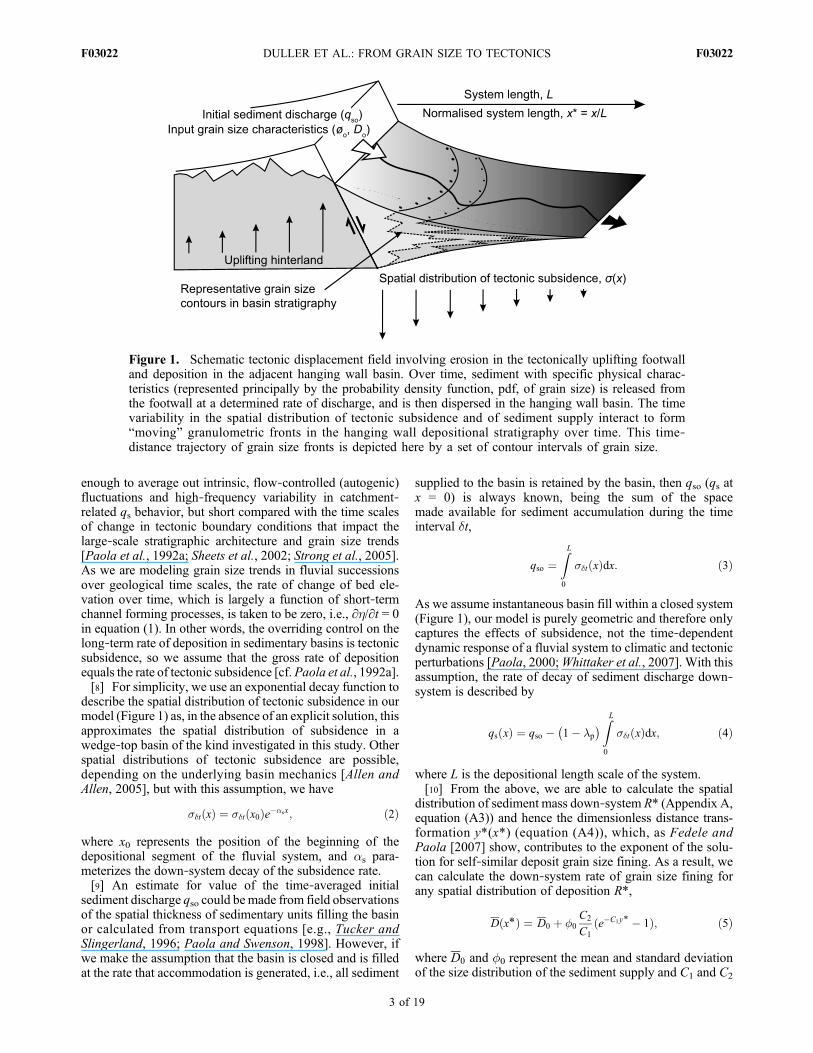
Figure 1. Schematic tectonic displacement field involving erosion in the tectonically uplifting footwalland deposition in the adjacent hanging wall basin. Over time, sediment with specific physical charac-teristics (represented principally by the probability density function, pdf, of grain size) is released fromthe footwall at a determined rate of discharge, and is then dispersed in the hanging wall basin. The timevariability in the spatial distribution of tectonic subsidence and of sediment supply interact to form“moving” granulometric fronts in the hanging wall depositional stratigraphy over time. This time‐distance trajectory of grain size fronts is depicted here by a set of contour intervals of grain size.

DULLER ET AL.: FROM GRAIN SIZE TO TECTONICS F03022F03022

3 of 19

are constants that, physically, express the relative partitioningof the variability in gravel supply into that arising from sys-tematic down‐system change in mean grain size (C2) and thevariation at a site (C1) [Fedele and Paola, 2007]. A fullderivation is given in Appendix A.[11] The model setup, described above, means that only a

small set of input parameters is required: (1) knowledge ofthe dimensional model space, which in this case equates todepositional system length; (2) knowledge of the rate of sub-sidence at x = 0 (so) and the spatial decay of the rate of sub-sidence (s(x)); (3) an estimate of the initial sediment dischargeqso; and (4) knowledge or reconstruction of the input grainsize distribution (mean Do and standard deviation �o).

2.2. Model Requirements and Assumptions

[12] It is important to recognize that a number of assump-tions and simplifications are either implicit or explicit inthe grain size fining model. We assume that (1) the systemmust be depositional along its entire length if down‐systemfining is to take place and (2) deposits must be the productof streamflow processes and not debris flow processes sothat selective transportation of individual particles can beunambiguously inferred. The following limitations are noted:(3) the self‐similar solutions used are strictly only valid forunimodal grain size distributions, (4) the mechanical break-down of particles (abrasion) is unaccounted for, (5) there canbe no additional lateral inputs of sediment other than thatat the upstream boundary, and (6) predictions are limited totwo‐dimensional distributions of grain size; the model doesnot replicate the full three‐dimensional lateral variation ofgrain size nor describe the details of facies partitioning ofgrain sizes down‐system.[13] Some of these assumptions are more limiting than

others. It is generally easy to identify fluvial deposits instratigraphy that have a unimodal grain size distribution,and most workers agree that selective deposition/transportdominates abrasion in setting regional trends in sedimentcaliber [e.g., Paola and Seal, 1995; Hoey and Bluck, 1999].In contrast, long length scale fluvial systems may have sub-stantial tributary junctions that reset fluvial grain size trendsand display significant facies partitioning between deposi-tional environments [Rice, 1998; Frings, 2008]. In suchcases, a simple application of the model may be problematicunless explicitly incorporating additional sediment inputs orrecognizing that the model only outputs “average” grainsizes for down‐system stratigraphy. See section 8 for furtherdiscussion. To avoid these potential complications, we havechosen to apply the fining model to fluvial successions of arelatively simple sediment routing system, a streamflow‐dominated alluvial fan. Such deposits are ideal for an initialfield application because (i) they receive sediment from apoint source and are not usually in receipt of additionalsediment down‐system, (ii) the two‐dimensional applicationof the model is a reasonable simplification for the radialdistribution of sediment found in such settings, and (iii)there is little or no facies partitioning in the gravel units.[14] In addition to the points above, we note further

simplifications in our model formulation: (7) an exponentialdecrease in subsidence is used because this is a simple wayof varying the amplitude and wavelength of tectonic sub-sidence, as well as being typical for describing accommo-dation generation in foreland and wedge‐top basins [Allen

and Allen, 2005]; (8) a mass balance approach is adoptedto model our field data and so we assume a closed system,which is supported by the localization and geometry of theMontsor Fan Succession within the structurally restrictedPobla wedge‐top basin; and (9) our geometric modelingapproach invokes a fluvial system that is always at steadystate, so the transient dynamics of sediment routing systemsand transient stratigraphy are unaccounted for.

3. Sensitivity Analysis

[15] Before applying the model to field data, we first con-ducted a sensitivity analysis on the model by varying severalof the key parameters to explore their relative effects on theresultant spatial trend of mean grain size within stratigraphy.The parameters varied were (1) the initial value of sedimentdischarge qso, (2) the spatial distribution of subsidence s(x),(3) the constant of variance partitioning C1 (Appendix A,equation (A6)), and (4) the standard deviation of the sedimentsupply �o.

3.1. Varying the Initial Value of Sediment Dischargeand Spatial Distribution of Subsidence

[16] In order to explore the effects of varying sedimentdischarge and subsidence distribution on time‐averaged grainsize within stratigraphy, we first evaluate the case of a basinwith a fixed distribution of subsidence s(x) and a fixedsystem length L and vary initial values of sediment dis-charge qso. For the two‐dimensional system considered here,we define a dimensionless parameter Fqs, which representsthe ratio of qso to accommodation creation due to tectonicsubsidence, i.e.,

Fqs ¼ qsoRL0��t xð Þdx

: ð6Þ

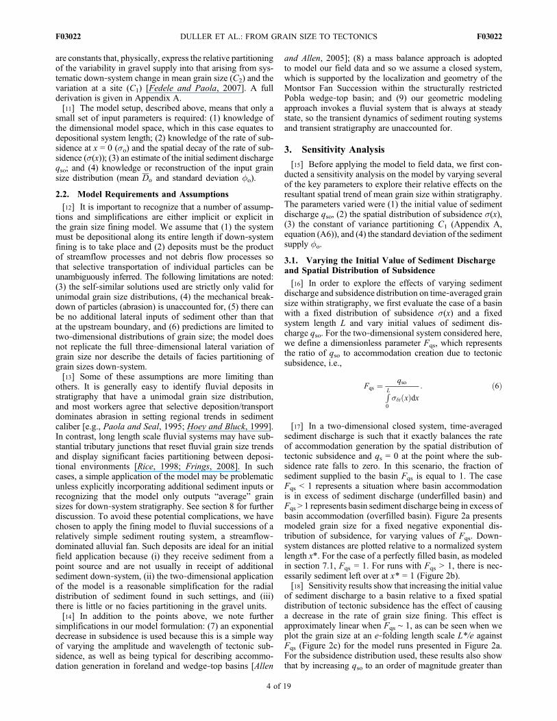
[17] In a two‐dimensional closed system, time‐averagedsediment discharge is such that it exactly balances the rateof accommodation generation by the spatial distribution oftectonic subsidence and qs = 0 at the point where the sub-sidence rate falls to zero. In this scenario, the fraction ofsediment supplied to the basin Fqs is equal to 1. The caseFqs < 1 represents a situation where basin accommodationis in excess of sediment discharge (underfilled basin) andFqs > 1 represents basin sediment discharge being in excess ofbasin accommodation (overfilled basin). Figure 2a presentsmodeled grain size for a fixed negative exponential dis-tribution of subsidence, for varying values of Fqs. Down‐system distances are plotted relative to a normalized systemlength x*. For the case of a perfectly filled basin, as modeledin section 7.1, Fqs = 1. For runs with Fqs > 1, there is nec-essarily sediment left over at x* = 1 (Figure 2b).[18] Sensitivity results show that increasing the initial value

of sediment discharge to a basin relative to a fixed spatialdistribution of tectonic subsidence has the effect of causinga decrease in the rate of grain size fining. This effect isapproximately linear when Fqs ∼ 1, as can be seen when weplot the grain size at an e‐folding length scale L*/e againstFqs (Figure 2c) for the model runs presented in Figure 2a.For the subsidence distribution used, these results also showthat by increasing qso to an order of magnitude greater than

DULLER ET AL.: FROM GRAIN SIZE TO TECTONICS F03022F03022

4 of 19

the reference case (Fqs = 1), the rate of down‐system finingbecomes negligible and is insensitive to subsequent increasesin the value of Fqs. This type of behavior may explain sheet‐like sedimentary units that characterize far‐field gravel trans-port [cf. Heller and Paola, 1989; Paola et al., 1992a] and

suggests that preserved grain size trends in these units shouldnot be significantly affected by fluctuations in the absolutemagnitude of qso.[19] In our second set of model runs, initial sediment

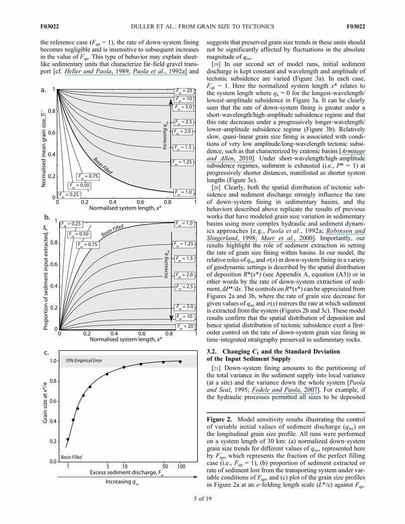
discharge is kept constant and wavelength and amplitude oftectonic subsidence are varied (Figure 3a). In each case,Fqs = 1. Here the normalized system length x* relates tothe system length where qs = 0 for the longest‐wavelength/lowest‐amplitude subsidence in Figure 3a. It can be clearlyseen that the rate of down‐system fining is greater under ashort‐wavelength/high‐amplitude subsidence regime and thatthis rate decreases under a progressively longer‐wavelength/lower‐amplitude subsidence regime (Figure 3b). Relativelyslow, quasi‐linear grain size fining is associated with condi-tions of very low amplitude/long‐wavelength tectonic subsi-dence, such as that characterized by cratonic basins [Armitageand Allen, 2010]. Under short‐wavelength/high‐amplitudesubsidence regimes, sediment is exhausted (i.e., P* = 1) atprogressively shorter distances, manifested as shorter systemlengths (Figure 3c).[20] Clearly, both the spatial distribution of tectonic sub-

sidence and sediment discharge strongly influence the rateof down‐system fining in sedimentary basins, and thebehaviors described above replicate the results of previousworks that have modeled grain size variation in sedimentarybasins using more complex hydraulic and sediment dynam-ics approaches [e.g., Paola et al., 1992a; Robinson andSlingerland, 1998; Marr et al., 2000]. Importantly, ourresults highlight the role of sediment extraction in settingthe rate of grain size fining within basins. In our model, therelative roles of qso and s(x) in down‐system fining in a varietyof geodynamic settings is described by the spatial distributionof deposition R*(x*) (see Appendix A, equation (A3)) or inother words by the rate of down‐system extraction of sedi-ment, dP*/dx. The controls onR*(x*) can be appreciated fromFigures 2a and 3b, where the rate of grain size decrease forgiven values of qso and s(x) mirrors the rate at which sedimentis extracted from the system (Figures 2b and 3c). These modelresults confirm that the spatial distribution of deposition andhence spatial distribution of tectonic subsidence exert a first‐order control on the rate of down‐system grain size fining intime‐integrated stratigraphy preserved in sedimentary rocks.

3.2. Changing C1 and the Standard Deviationof the Input Sediment Supply

[21] Down‐system fining amounts to the partitioning ofthe total variance in the sediment supply into local variance(at a site) and the variance down the whole system [Paolaand Seal, 1995; Fedele and Paola, 2007]. For example, ifthe hydraulic processes permitted all sizes to be deposited

Figure 2. Model sensitivity results illustrating the controlof variable initial values of sediment discharge (qso) onthe longitudinal grain size profile. All runs were performedon a system length of 30 km: (a) normalized down‐systemgrain size trends for different values of qso, represented hereby Fqs, which represents the fraction of the perfect fillingcase (i.e., Fqs = 1), (b) proportion of sediment extracted orrate of sediment lost from the transporting system under var-iable conditions of Fqs, and (c) plot of the grain size profilesin Figure 2a at an e‐folding length scale (L*/e) against Fqs.

DULLER ET AL.: FROM GRAIN SIZE TO TECTONICS F03022F03022

5 of 19

at each site in the same proportion as in the supply, then, ifinput size distribution were uniform, so would be thedistribution at every location, and hence, there would belocal size variability (high variance at each location) but nodown‐system fining. On the other hand, if local hydraulicselectivity was perfect, there would be strong down‐system

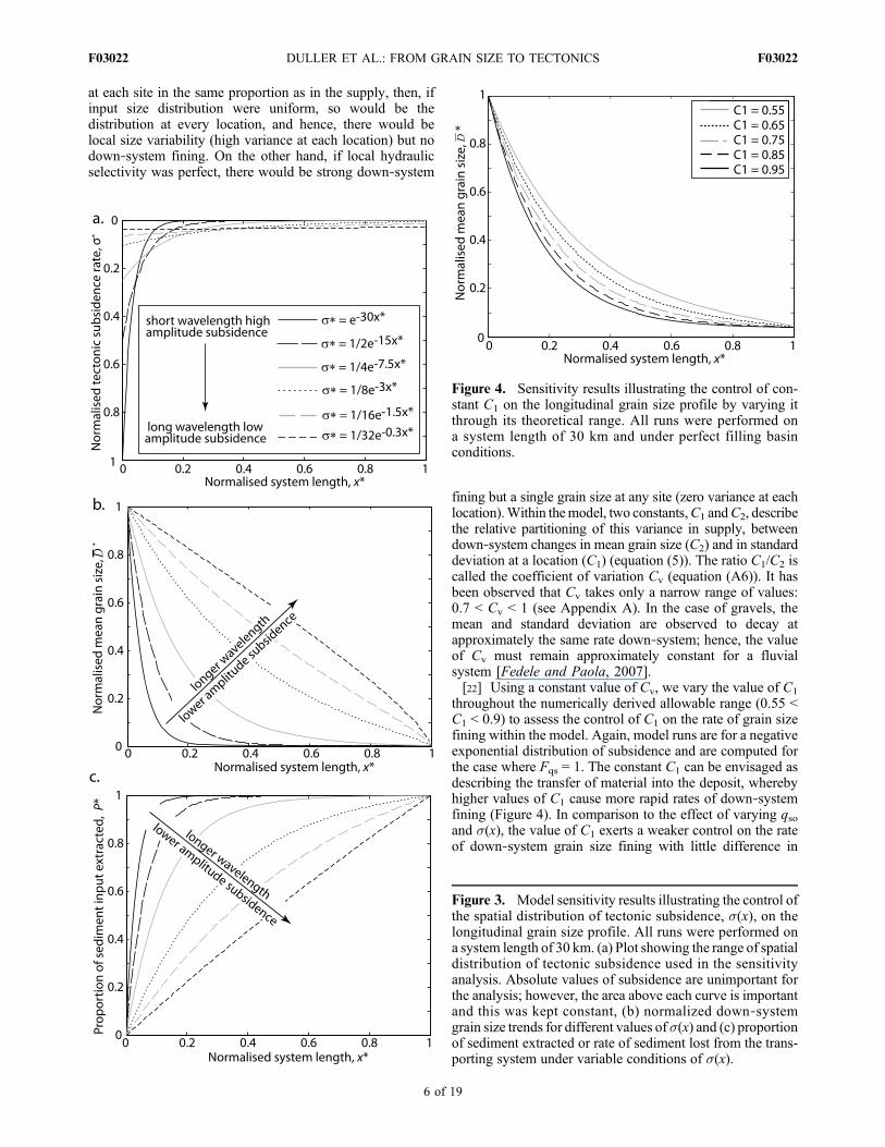
fining but a single grain size at any site (zero variance at eachlocation).Within themodel, two constants,C1 andC2, describethe relative partitioning of this variance in supply, betweendown‐system changes in mean grain size (C2) and in standarddeviation at a location (C1) (equation (5)). The ratio C1/C2 iscalled the coefficient of variation Cv (equation (A6)). It hasbeen observed that Cv takes only a narrow range of values:0.7 < Cv < 1 (see Appendix A). In the case of gravels, themean and standard deviation are observed to decay atapproximately the same rate down‐system; hence, the valueof Cv must remain approximately constant for a fluvialsystem [Fedele and Paola, 2007].[22] Using a constant value of Cv, we vary the value of C1

throughout the numerically derived allowable range (0.55 <C1 < 0.9) to assess the control of C1 on the rate of grain sizefining within the model. Again, model runs are for a negativeexponential distribution of subsidence and are computed forthe case where Fqs = 1. The constant C1 can be envisaged asdescribing the transfer of material into the deposit, wherebyhigher values of C1 cause more rapid rates of down‐systemfining (Figure 4). In comparison to the effect of varying qsoand s(x), the value of C1 exerts a weaker control on the rateof down‐system grain size fining with little difference in

Figure 3. Model sensitivity results illustrating the control ofthe spatial distribution of tectonic subsidence, s(x), on thelongitudinal grain size profile. All runs were performed ona system length of 30 km. (a) Plot showing the range of spatialdistribution of tectonic subsidence used in the sensitivityanalysis. Absolute values of subsidence are unimportant forthe analysis; however, the area above each curve is importantand this was kept constant, (b) normalized down‐systemgrain size trends for different values of s(x) and (c) proportionof sediment extracted or rate of sediment lost from the trans-porting system under variable conditions of s(x).

Figure 4. Sensitivity results illustrating the control of con-stant C1 on the longitudinal grain size profile by varying itthrough its theoretical range. All runs were performed ona system length of 30 km and under perfect filling basinconditions.

DULLER ET AL.: FROM GRAIN SIZE TO TECTONICS F03022F03022

6 of 19

predicted grain size in the proximal and distal parts of thesystem. For intermediate‐system lengths, e.g., x* = 0.4, thenormalized mean grain size varies from 0.15 to 0.3 acrossthe range for C1 modeled here.[23] Another parameter that affects the spatial distribution

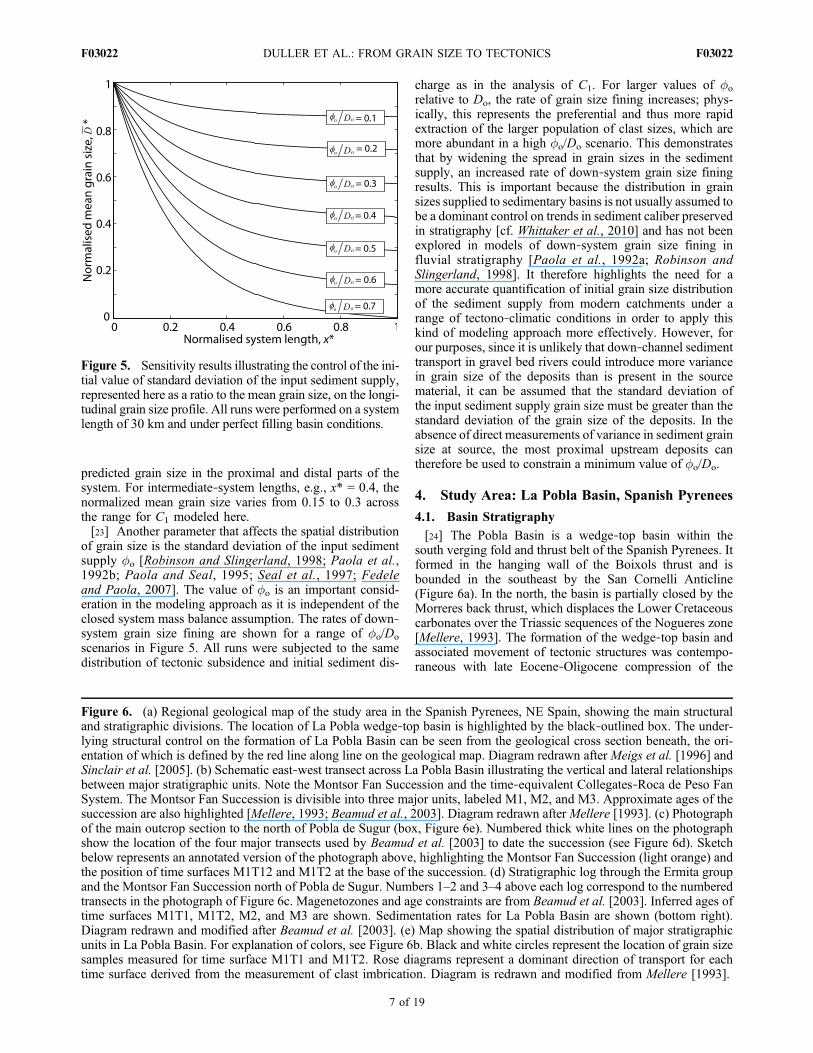
of grain size is the standard deviation of the input sedimentsupply �o [Robinson and Slingerland, 1998; Paola et al.,1992b; Paola and Seal, 1995; Seal et al., 1997; Fedeleand Paola, 2007]. The value of �o is an important consid-eration in the modeling approach as it is independent of theclosed system mass balance assumption. The rates of down‐system grain size fining are shown for a range of �o/Do

scenarios in Figure 5. All runs were subjected to the samedistribution of tectonic subsidence and initial sediment dis-

charge as in the analysis of C1. For larger values of �o

relative to Do, the rate of grain size fining increases; phys-ically, this represents the preferential and thus more rapidextraction of the larger population of clast sizes, which aremore abundant in a high �o/Do scenario. This demonstratesthat by widening the spread in grain sizes in the sedimentsupply, an increased rate of down‐system grain size finingresults. This is important because the distribution in grainsizes supplied to sedimentary basins is not usually assumed tobe a dominant control on trends in sediment caliber preservedin stratigraphy [cf. Whittaker et al., 2010] and has not beenexplored in models of down‐system grain size fining influvial stratigraphy [Paola et al., 1992a; Robinson andSlingerland, 1998]. It therefore highlights the need for amore accurate quantification of initial grain size distributionof the sediment supply from modern catchments under arange of tectono‐climatic conditions in order to apply thiskind of modeling approach more effectively. However, forour purposes, since it is unlikely that down‐channel sedimenttransport in gravel bed rivers could introduce more variancein grain size of the deposits than is present in the sourcematerial, it can be assumed that the standard deviation ofthe input sediment supply grain size must be greater than thestandard deviation of the grain size of the deposits. In theabsence of direct measurements of variance in sediment grainsize at source, the most proximal upstream deposits cantherefore be used to constrain a minimum value of �o/Do.

4. Study Area: La Pobla Basin, Spanish Pyrenees

4.1. Basin Stratigraphy

[24] The Pobla Basin is a wedge‐top basin within thesouth verging fold and thrust belt of the Spanish Pyrenees. Itformed in the hanging wall of the Boixols thrust and isbounded in the southeast by the San Cornelli Anticline(Figure 6a). In the north, the basin is partially closed by theMorreres back thrust, which displaces the Lower Cretaceouscarbonates over the Triassic sequences of the Nogueres zone[Mellere, 1993]. The formation of the wedge‐top basin andassociated movement of tectonic structures was contempo-raneous with late Eocene‐Oligocene compression of the

Figure 5. Sensitivity results illustrating the control of the ini-tial value of standard deviation of the input sediment supply,represented here as a ratio to the mean grain size, on the longi-tudinal grain size profile. All runs were performed on a systemlength of 30 km and under perfect filling basin conditions.

Figure 6. (a) Regional geological map of the study area in the Spanish Pyrenees, NE Spain, showing the main structuraland stratigraphic divisions. The location of La Pobla wedge‐top basin is highlighted by the black‐outlined box. The under-lying structural control on the formation of La Pobla Basin can be seen from the geological cross section beneath, the ori-entation of which is defined by the red line along line on the geological map. Diagram redrawn after Meigs et al. [1996] andSinclair et al. [2005]. (b) Schematic east‐west transect across La Pobla Basin illustrating the vertical and lateral relationshipsbetween major stratigraphic units. Note the Montsor Fan Succession and the time‐equivalent Collegates‐Roca de Peso FanSystem. The Montsor Fan Succession is divisible into three major units, labeled M1, M2, and M3. Approximate ages of thesuccession are also highlighted [Mellere, 1993; Beamud et al., 2003]. Diagram redrawn afterMellere [1993]. (c) Photographof the main outcrop section to the north of Pobla de Sugur (box, Figure 6e). Numbered thick white lines on the photographshow the location of the four major transects used by Beamud et al. [2003] to date the succession (see Figure 6d). Sketchbelow represents an annotated version of the photograph above, highlighting the Montsor Fan Succession (light orange) andthe position of time surfaces M1T12 and M1T2 at the base of the succession. (d) Stratigraphic log through the Ermita groupand the Montsor Fan Succession north of Pobla de Sugur. Numbers 1–2 and 3–4 above each log correspond to the numberedtransects in the photograph of Figure 6c. Magenetozones and age constraints are from Beamud et al. [2003]. Inferred ages oftime surfaces M1T1, M1T2, M2, and M3 are shown. Sedimentation rates for La Pobla Basin are shown (bottom right).Diagram redrawn and modified after Beamud et al. [2003]. (e) Map showing the spatial distribution of major stratigraphicunits in La Pobla Basin. For explanation of colors, see Figure 6b. Black and white circles represent the location of grain sizesamples measured for time surface M1T1 and M1T2. Rose diagrams represent a dominant direction of transport for eachtime surface derived from the measurement of clast imbrication. Diagram is redrawn and modified from Mellere [1993].

DULLER ET AL.: FROM GRAIN SIZE TO TECTONICS F03022F03022

7 of 19

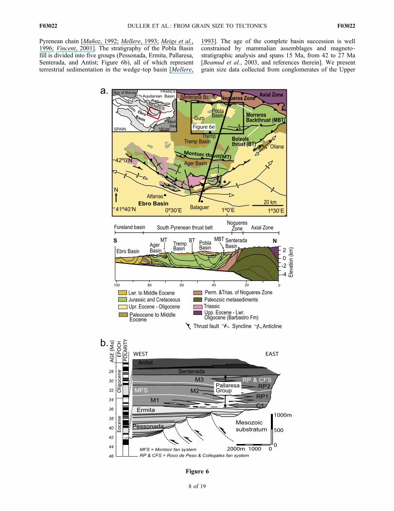
Pyrenean chain [Muñoz, 1992; Mellere, 1993; Meigs et al.,1996; Vincent, 2001]. The stratigraphy of the Pobla Basinfill is divided into five groups (Pessonada, Ermita, Pallaresa,Senterada, and Antist; Figure 6b), all of which representterrestrial sedimentation in the wedge‐top basin [Mellere,

1993]. The age of the complete basin succession is wellconstrained by mammalian assemblages and magneto‐stratigraphic analysis and spans 15 Ma, from 42 to 27 Ma[Beamud et al., 2003, and references therein]. We presentgrain size data collected from conglomerates of the Upper

Figure 6

DULLER ET AL.: FROM GRAIN SIZE TO TECTONICS F03022F03022

8 of 19

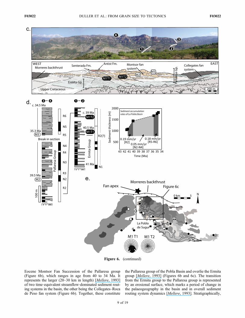
Eocene Montsor Fan Succession of the Pallaresa group(Figure 6b), which ranges in age from 40 to 34 Ma. Itrepresents the larger (20–30 km in length) [Mellere, 1993]of two time‐equivalent streamflow‐dominated sediment rout-ing systems in the basin, the other being the Collegates–Rocade Peso fan system (Figure 6b). Together, these constitute

the Pallaresa group of the Pobla Basin and overlie the Ermitagroup [Mellere, 1993] (Figures 6b and 6c). The transitionfrom the Ermita group to the Pallaresa group is representedby an erosional surface, which marks a period of change inthe palaeogeography in the basin and in overall sedimentrouting system dynamics [Mellere, 1993]. Stratigraphically,

Figure 6. (continued)

DULLER ET AL.: FROM GRAIN SIZE TO TECTONICS F03022F03022

9 of 19

this transition is expressed by the upward passage of athinly bedded (∼5–10 m) fan delta‐lacustrine‐floodplainsuccession, composed entirely of locally derived Mesozoiclimestone material [Mellere, 1993], to a thickly bedded andamalgamated alluvial fan succession (Figure 6c) that containsclasts indicative of a source area within the Nogueres andAxial zones (Figure 6a). The scales of the depositional sys-tems also differ significantly, while the Ermita depositionalsystem was represented by small alluvial fans progradinginto small lakes over a period of ca. 1.5 Ma, the Montsordepositional system was represented by the progradation ofspatially extensive alluvial fans over a period of ca. 6 Ma,largely filling the wedge‐top basin. Consequently, theMontsorFan Succession represents a major period of change in sedi-ment routing system dynamics, related to an intense episodeof thrust activity within the antiformal stack of the Nogueresand Axial zones [Mellere, 1993; Vincent, 2001]. Activity ofthis sort played a crucial role in governing temporal patternsof sediment yield and supply to adjacent basins [Morris et al.,1998; Vincent, 1999] and also influenced patterns of tectonicsubsidence in adjacent basins [Beamud et al., 2003].[25] The Montsor Fan Succession is divided by Mellere

[1993] into three major units ( M1, M2, and M3), each one∼200–400 m in thickness and bounded by a major lacustrineinterval (Figures 6b and 6c). Here we focus on the lowerunit M1, and we further divide it into two separate units,M1T1 and M1T2, which are separated by a lacustrine hori-zon, traceable across the length of the basin. The conglom-erates of the Montsor Fan Succession are cobble to bouldergrade, clast supported, and moderately sorted to well sortedand show well‐developed imbrication. These local features,togetherwith the presence of upward‐fining units and commongutter casts, indicate the dominance of turbulent streamflowprocesses, a prerequisite for applying the selective depositionmodel of Fedele and Paola [2007].

4.2. Constraints on Sediment Deposition Rates

[26] Beamud et al. [2003], using magneto‐stratigraphicdata from samples collected at a location 5 km north ofPobla de Segur (magneto‐stratigraphic transect shown onFigure 6c), calculate sediment accumulation rates for theMontsor Fan Succession on the order of 0.05 mm yr−1 from∼40 to 35.5 Ma, coinciding with the deposition of unitsM1T1, M1T2, and M2 (Figure 6d). In this paper, we presentdata from units M1T1 and M1T2 only, with thicknessesof ∼75 and ∼150 m directly north of Pobla de Segur(Figure 6c) and separation by a thickness of stratigraphyof ∼25 m. The deposition of unit M1T1 took place syn-chronously with a marked decrease in the rate of tectonicsubsidence (Figure 6d) in this part of the Pobla Basin duringan episode of major tectonic reorganization [Beamud et al.,2003]. A detailed comparison of our time lines with thismagneto‐stratigraphic data suggests that time surface M1T1has an absolute stratigraphic age of 40.5 Ma (Beamud, per-sonal communication). Using the published sediment accu-mulation rate of 0.05 mm yr−1 for this time period, thethickness of ∼25 m that separates M1T1 and M1T2 suggestsan intervening time period of 0.5 Ma, giving an age of ca.40 Ma for M1T2 (Figure 6d).[27] The Montsor Fan Succession provides an excellent

natural laboratory to investigate the dynamics of time‐integrated grain size variation in fluvial stratigraphy because

of (1) excellent exposure over the entire length of the fansystem, allowing collection of grain size data and the infer-ence of system length; (2) the presence of laterally extensivelacustrine and paleosol horizons that enable correlative hor-izons or “time surfaces” to be traced across the basin; (3) aconstraint on local sediment accumulation rates (and hencetectonic subsidence rates) frommagneto‐stratigraphy [Beamudet al., 2003]; (4) the geometry and structural restriction ofLa Pobla wedge‐top basin, as inferred from the distributionof the Montsor Fan Succession [Mellere, 1993], whichenables us to be confident in our closed system modelingassumption for the gravel fraction; (5) the recognition ofsedimentary features that are associated with turbulent,fluvial sediment transport and deposition; (6) the wedgeshape geometry of major sedimentary units (fan lobes) andpalaeoflow directions, which supports a point source sedi-ment delivery to the system with no additional sedimentinput down‐system; and (7) knowledge of the location of thefan apex (x = 0) over time in order to establish an absolutedistance for each grain size measurement (Figure 6e).

5. Methods: Data Collection and Analysis

[28] As this study attempts to explain the trends in grainsize in preserved fluvial stratigraphy, it is necessary to collectgrain size data that (1) is representative of a significant periodof geological time and (2) follows units along discrete timehorizons or time surfaces. The former requirement means thatthe details of individual flows and high‐frequency climaticvariations are integrated and therefore “smoothed out” overgeological time, essential if the quantitative model is to beapplied. For documented sediment accumulation rates in theMontsor Fan Succession on the order 0.05 mm yr−1, ∼5 m ofstratigraphy would be accumulated in 105 years.We thereforechose to consider grain size variations within ∼10 m of ver-tical stratigraphy at each sample site, therefore averaginggrain size in stratigraphy over time periods of ∼0.2 Ma. Togain an accurate representation of the spatial arrangement ofgrain size trends in stratigraphy without incorporating short‐term temporal variations, it is essential that sample locationsfollow key time surfaces. Although the term “time surface” isnot be applicable over the short term, e.g., <104 years, due todiachroneity, it is applicable here as we are sampling grainsize over a substantial period of geological time and so limitpotential diachroneity. Time surfaces were defined severalmeters above the base and below the top of major strati-graphic units in order to limit the uncertainty in grain sizevalues that may result purely from fan lobe establishment.We present spatial grain size data for two time surfaces at thebase of unit M1T1 and the base of unit M1T2 (Figure 6e).[29] Sampling the outcrop for grain size distribution

involved the random selection and measurement of the longand short axis of 100 clasts, > 2 mm, within a 1 m2 samplearea [Wolman, 1954; Stock et al., 2008]. This was under-taken both manually and digitally, using scaled photographs[Buscombe, 2008;Whittaker et al., 2010], with both methodsproducing statistically similar distributions. There are variousways to estimate a time‐averaged grain size distributioncurve for the 10 m2 area without sampling the entire area.Given a physically based assumption for a theoretical prob-ability distribution, in this case lognormal, the best robustestimate is a least squares fit to estimates of the most widely

DULLER ET AL.: FROM GRAIN SIZE TO TECTONICS F03022F03022

10 of 19

spaced points on the distribution. To obtain a three‐pointestimate, we therefore measured the visually finest, inter-mediate, and coarsest 1 m2 areas within the 10 m2 area andfitted a lognormal pdf (probability density function) to gen-erate a representative curve for the 10 m2 area.

6. Grain Size Data

6.1. Observations

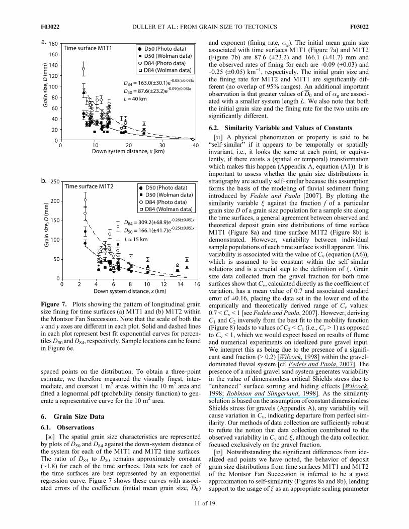
[30] The spatial grain size characteristics are representedby plots of D50 and D84 against the down‐system distance ofthe system for each of the M1T1 and M1T2 time surfaces.The ratio of D84 to D50 remains approximately constant(∼1.8) for each of the time surfaces. Data sets for each ofthe time surfaces are best represented by an exponentialregression curve. Figure 7 shows these curves with associ-ated errors of the coefficient (initial mean grain size, D0)

and exponent (fining rate, ag). The initial mean grain sizeassociated with time surfaces M1T1 (Figure 7a) and M1T2(Figure 7b) are 87.6 (±23.2) and 166.1 (±41.7) mm andthe observed rates of fining for each are ‐0.09 (±0.03) and‐0.25 (±0.05) km−1, respectively. The initial grain size andthe fining rate for M1T2 and M1T1 are significantly dif-ferent (no overlap of 95% ranges). An additional importantobservation is that greater values of D0 and of ag are associ-ated with a smaller system length L. We also note that boththe initial grain size and the fining rate for the two units aresignificantly different.

6.2. Similarity Variable and Values of Constants

[31] A physical phenomenon or property is said to be“self‐similar” if it appears to be temporally or spatiallyinvariant, i.e., it looks the same at each point, or equiva-lently, if there exists a (spatial or temporal) transformationwhich makes this happen (Appendix A, equation (A1)). It isimportant to assess whether the grain size distributions instratigraphy are actually self‐similar because this assumptionforms the basis of the modeling of fluvial sediment finingintroduced by Fedele and Paola [2007]. By plotting thesimilarity variable x against the fraction f of a particulargrain size D of a grain size population for a sample site alongthe time surfaces, a general agreement between observed andtheoretical deposit grain size distributions of time surfaceM1T1 (Figure 8a) and time surface M1T2 (Figure 8b) isdemonstrated. However, variability between individualsample populations of each time surface is still apparent. Thisvariability is associated with the value of Cv (equation (A6)),which is assumed to be constant within the self‐similarsolutions and is a crucial step to the definition of x. Grainsize data collected from the gravel fraction for both timesurfaces show that Cv, calculated directly as the coefficient ofvariation, has a mean value of 0.7 and associated standarderror of ±0.16, placing the data set in the lower end of theempirically and theoretically derived range of Cv values:0.7 < Cv < 1 [see Fedele and Paola, 2007]. However, derivingC1 and C2 inversely from the best fit to the mobility function(Figure 8) leads to values of C2 < C1 (i.e., Cv > 1) as opposedto Cv < 1, which we would expect based on results of flumeand numerical experiments on idealized pure gravel input.We interpret this as being due to the presence of a signifi-cant sand fraction (> 0.2) [Wilcock, 1998] within the gravel‐dominated fluvial system [cf. Fedele and Paola, 2007]. Thepresence of a mixed gravel sand system generates variabilityin the value of dimensionless critical Shields stress due to“enhanced” surface sorting and hiding effects [Wilcock,1998; Robinson and Slingerland, 1998]. As the similaritysolution is based on the assumption of constant dimensionlessShields stress for gravels (Appendix A), any variability willcause variation in Cv, indicating departure from perfect sim-ilarity. Our methods of data collection are sufficiently robustto refute the notion that data collection contributed to theobserved variability in Cv and x, although the data collectionfocused exclusively on the gravel fraction.[32] Notwithstanding the significant differences from ide-

alized end points we have noted, the behavior of depositgrain size distributions from time surfaces M1T1 and M1T2of the Montsor Fan Succession is inferred to be a goodapproximation to self‐similarity (Figures 8a and 8b), lendingsupport to the usage of x as an appropriate scaling parameter

Figure 7. Plots showing the pattern of longitudinal grainsize fining for time surfaces (a) M1T1 and (b) M1T2 withinthe Montsor Fan Succession. Note that the scale of both thex and y axes are different in each plot. Solid and dashed linesin each plot represent best fit exponential curves for percen-tilesD50 andD84, respectively. Sample locations can be foundin Figure 6e.

DULLER ET AL.: FROM GRAIN SIZE TO TECTONICS F03022F03022

11 of 19

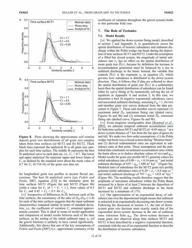
for longitudinal grain size profiles in ancient fluvial suc-cessions. The best fit analytical curve [see Fedele andPaola, 2007, equation (23)] to the similarity plots fortime surfaces M1T1 (Figure 8a) and M1T2 (Figure 8b)yields a value for Cv of 1 < Cv < 1.1, from values of 0.5for C1 and 0.45 < C2 < 0.5 for C2.[33] Irrespective of differences in D0 between each of the

time surfaces, the consistency of the ratio of D84/D50 (∼1.8)for each of the time surfaces suggests that the input sedimentcharacteristics remained similar in terms of standard devia-tion, i.e., the coefficient of variation Cv remained approxi-mately constant. This is ideal in terms of model applicationand comparison of model results between each of the timesurfaces, as the sorting of the initial sediment input �o (ofthe gravel fraction) is unlikely to have varied significantly.Additionally, this shows that one of the key assumptions ofFedele and Paola [2007] (i.e., approximate constancy of the

coefficient of variation throughout the gravel system) holdsin this particular field case.

7. The Role of Tectonics

7.1. Model Results

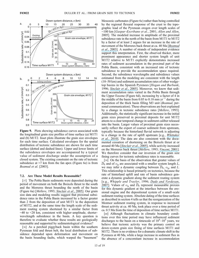
[34] We applied the down‐system fining model, describedin section 2 and Appendix A, to quantitatively assess thespatial distribution of tectonic subsidence and sediment dis-charge within the Pobla wedge‐top basin during the deposi-tion of time surfaces M1T1 andM1T2. Under the assumptionof a filled but closed system, the magnitude of initial sub-sidence rate so has no effect on the spatial distribution ofmean grain size DðxÞ, because by definition the increase inaccommodation generation must be balanced by a rise insediment discharge to the basin. Instead, the variable thatcontrols DðxÞ is the exponent as in equation (2), whichgoverns how subsidence is distributed in the down‐systemdirection. Thus, it follows that if data are collected to showthe spatial distribution of grain size DðxÞ in a sedimentarybasin then the spatial distribution of subsidence can be foundeither by curve fitting or by numerically solving the set ofequations in Appendix A and section 2. In this case, wedetermine a best fit negative exponential subsidence curveand associated sediment discharge, assuming Fqs = 1, for twoend‐member grain size curves deduced from the data pre-sented in Figure 7. These end‐member curves represent (1)maximum initial D0, maximum fining rate (dotted curve,Figures 9a and 9b) and (2) minimum initial D0, minimumfining rate (dashed curve, Figures 9a and 9b).[35] From magneto‐stratigraphic data [Beamud et al.,

2003], we estimate temporal sediment accumulation ratesfor both time surfaces M1T1 andM1T2 of ∼0.05 mm yr−1 at adown‐system distance of 7 km from the fan apex (Figures 6cand 6d). We make two first‐order assumptions: (1) the Poblawedge‐top basin was a closed system during “Montsor times”and (2) derived sedimentation rates are equivalent to sub-sidence rates at that point. These assumptions and the pub-lished data constraints on sediment accumulation rates withinthe basin allow us to deduce absolute values of s(x) and qso.Model results for grain size profile M1T1 generate values forinitial subsidence rate of 0.08 < so < 0.16 mm yr−1 and initialsediment discharge of 655 < qso < 688 m2 kyr−1 (Figure 9a).Modeled rates of subsidence for the M1T2 grain size profilegenerate initial subsidence rates of 0.29 < so < 0.8 mm yr−1

and initial sediment discharge of 797 < qso < 1433 m2 kyr−1

(Figure 9b). The modeling results therefore suggest that theamplitude of maximum subsidence within the Pobla Basinincreased by a factor of at least 2 between the deposition ofM1T1 and M1T2 and sediment discharge to the basinincreased by a minimum of 17%.[36] Our approximation of an exponential decay of sub-

sidence rate over the depositional length means that sedimentis extracted at an exponentially decreasing rate down‐system.Following the discussion in section 3.1, the rate of down‐system grain size decrease must exactly match that of theexponential down‐system decrease in the rate of sedimentmass extraction from qso. The down‐system decrease inmean grain size observed along time surfaces M1T1 andM1T2 is best described by a negative exponential function,consistent with the use of an exponential function to describethe distribution of tectonic subsidence.

Figure 8. Plots showing the approximate self‐similardeposit grain size distributions of all grain size samplestaken from time surfaces (a) M1T1 and (b) M1T2. Thickblack lines represent the analytical fit to all grain size sam-ples for each time surface. The middle fit represents the bestfit analytical curve to each data set, i.e., Cv = 0.7. The lowerand upper analytical fits represent upper and lower limits ofCv as defined by the standard error about the mean value of0.7 for Cv (0.7±0.16) of the grain size data set.

DULLER ET AL.: FROM GRAIN SIZE TO TECTONICS F03022F03022

12 of 19

7.2. Are These Model Results Reasonable?

[37] The Pobla Basin sediments were deposited during theperiod of movement on both the Boixols thrust to the southand the Morreres thrust bounding the north of the basin(Figure 6a) [Mellere, 1993; Sinclair et al., 2005]. Our grainsize data and modeling results suggest that proximal subsi-dence rates in the Pobla Basin increased by a factor greaterthan 2 from the deposition of unit M1T1 to the depositionof M1T2, and at the same time the length scale of the sedi-ment routing system shortened by a similar factor from∼40 to <20 km, consistent with higher‐amplitude, shorter‐wavelength subsidence in the basin. A key question istherefore to evaluate whether these results are geologicallyreasonable and supported by sedimentological evidence?[38] As a perched piggyback basin within the southern

Pyrenean fold and thrust belt, the local distribution of sub-sidence depended upon deformation and movement onthe basin bounding faults, which warped the “basement”

Mesozoic carbonates (Figure 6c) rather than being controlledby the regional flexural response of the crust to the topo-graphic load of the Pyrenean orogen over length scales of∼100 km [Gaspar‐Escribano et al., 2001; Allen and Allen,2005]. The modeled increase in amplitude of the proximalsubsidence rate in the north of the basin fromM1T1 to M1T2by a factor of at least 2 argues for an increase in the rate ofmovement of the Morreres back thrust at ca. 40 Ma [Beamudet al., 2003]. A number of strands of independent evidencesupport this interpretation. First, the observed thicker, moreprominent appearance and shorter system length of unitM1T2 relative to M1T1 explicitly demonstrates increasedrates of sediment accumulation in the proximal part of thePobla Basin, consistent with an increased rate of tectonicsubsidence to provide the accommodation space required.Second, the subsidence wavelengths and subsidence valuesestimated from the modeling are consistent with the length(10–50 km) and sediment accumulation rates of other wedge‐top basins in the Spanish Pyrenees [Hogan and Burbank,1996; Sinclair et al., 2005]. Moreover, we know that sedi-ment accumulation rates varied in the Pobla Basin throughthe Upper Eocene (Figure 6d), increasing by a factor of 4 inthe middle of the basin from 0.05 to 0.18 mm yr−1 during thedeposition of the thick basin filling M3 unit (Beamud, per-sonal communication). These observations are best explainedby a change in tectonic subsidence rates [Mellere, 1993].Additionally, the statistically significant increase in the initialgrain sizes preserved in proximal deposits for unit M1T2attests to a clear temporal change in sediment caliber releasedinto the basin. Larger values of proximal grain sizes neces-sarily reflect the export of coarser sediment from upstream,typically because the hinterland fluvial network is adjustingto a change in the rate of uplift upstream [e.g., Whittakeret al., 2010]. The data are also consistent with the docu-mented cessation of shortening on the Boixols thrust at oraround 40 Ma [Sinclair et al., 2005], while activity increasedon the Morreres back thrust [Mellere, 1993; Vincent, 2001].We therefore consider that our inversion of the grain sizefining curves for tectonic subsidence rates is reasonable.[39] On the basis of the observation that greater values of

D0 and of ag are associated with a smaller system length L,we may infer a dynamic coupling between D0, ag, and L.This relationship is based primarily on tectonics, because therate of hinterland uplift and rate of basin subsidence gen-erate a dynamic gradient along the sediment routing system[e.g., Whipple and Trayler, 1996; Dade and Verdeyan,2007]. Values of ag and D0 represent measurable proxiesfor this dynamic gradient at the interface between the ero-sional engine and the depositional system of a small‐scalesediment routing system. Absolute dating of the time surfacesas described in section 4 tells us that the reorganization of theMontsor sediment routing system, in response to increasedthrust activity at ca. 40 Ma, took place over a time period ofca. 0.5 Ma from the time of deposition of time surface M1T1.[40] Although fluctuations in climatic boundary condi-

tions over this time period may have influenced sedimentdischarges to the basin on a timescale of 104–105 years, webelieve that tectonic activity was the primary control ondown‐system grain size fining of time surfaces M1T1 andM1T2. There is no evidence for a dramatic climate shift in thePyrenees at 40 Ma, while a large increase in sediment flux inthe absence of a concomitant increase in accommodation

Figure 9. Plots showing subsidence curves associated withthe longitudinal grain size profiles of time surface (a) M1T1and (b) M1T2. Inset plots illustrate the grain size envelopesfor each time surface. Calculated envelopes for the spatialdistribution of tectonic subsidence are shown for each timesurface (dotted and dashed lines). Upper and lower limits ofthe subsidence envelopes are accompanied by a typicalvalue of sediment discharge under the assumption of aclosed system. The existing constraint on the rate of tectonicsubsidence at ≈7 km from the fan apex (Figure 6e) is fromBeamud et al. [2003].

DULLER ET AL.: FROM GRAIN SIZE TO TECTONICS F03022F03022

13 of 19

generation would result in the progradation of thinner, later-ally extensive units, which we do not see [cf. Heller andPaola, 1989, 1992].

8. Discussion and Future Work

[41] The ability to directly couple fluvial successions,expressed here in terms of down‐system variation in grainsize, with formative time‐averaged surface processes is acrucial step toward our understanding and quantification ofsediment routing system dynamics. Such insights are requiredif we are to predict the distribution of grain sizes in sedi-mentary basins or, conversely, if we are to invert grain sizetrends for key surface process and tectonic variables in a widerange of settings. Self‐similar solutions for down‐systemgrain size fining (Appendix A) are an important step towardfulfilling this goal, as they only require input parametersthat are readily attainable from stratigraphic field studies.While the development of the similarity solutions used heredepended on the results of fluvial process models over shorttime periods in order to define a relative mobility function, itis import to reiterate that these solutions are developed forfluvial successions over significant periods of geologicaltime.[42] By undertaking a sensitivity analysis of key para-

meters within the model, we are able to show the impact ofsediment discharge, the spatial distribution of tectonic sub-sidence (and hence the spatial distribution of deposition),input sediment supply characteristics, and “sediment transfer”constants C1 and C2 on the spatial trends in down‐systemgrain size. These results highlight the extent to which spatialtrends in sediment caliber in sedimentary basins can beinterpreted in terms of key controlling variables and providea basis for future application to a range of basin types withsignificantly different regimes of tectonic subsidence, sedi-ment discharge, and sediment supply characteristics. Ofparticular note is the fact that modeled grain size trends arevery sensitive to changes in the magnitude of sedimentsupply when the basin is approximately full (i.e., Fqs ∼ 1)but are relatively insensitive to fluctuations in sediment dis-charge when Fqs is large (i.e., > 10), and there is alreadysignificant bypass from the system. Such results are importantwhen considering sedimentation in areas where there is littleaccommodation generation. In general, the results of thesensitivity analysis are consistent with the results of morecomplex numerical models of down‐system grain size fining[e.g., Parker, 1991; Robinson and Slingerland, 1998] andhighlight the need to explore in more detail how the distri-bution of sediment size, in addition to the magnitude ofsupply, affects grain size trends in sedimentary basins [cf.Whittaker et al., 2010].[43] In particular, more theoretical and field data are needed

to further constrain the values of the “constants” C1 and C2,and hence Cv. In the original model, a range of numericalvalues for C1 (0.55 < C1 < 0.9) was determined fromnumerical experiments and limited field data [see Fedele andPaola, 2007]. Values of C1 and C2 within a given fluvialsystem are likely to be characterized by a specific section ofthis range, i.e., the values of C1 and C2 are unlikely to beuniversal [cf. Fedele and Paola, 2007]. Analytical best fits toour gravel (field) data set are provided by values of C2 < C1

(i.e., Cv > 1) as opposed to C1 < C2 (Cv < 1), derived from

flume and numerical experiments on idealized pure gravelinput. This is in contrast to a value for Cv of 0.7 ± 0.16obtained from the raw analysis of the field data set, whichwas undertaken on the gravel fraction only. We attributethis difference as being due to the presence of a significantsand fraction. While our field data are consistent with anapproximately self‐similar distribution of grain size down‐system, the impact of departures from this assumptionrequires further investigation. In addition, a combined theo-retical and field study that investigates the form of the simi-larity variable and the form of the relative mobility functionbetween the two idealized end‐members, pure gravel andpure sand, is needed.[44] We apply and validate the similarity solutions for

down‐system grain size fining using the Montsor Fan Suc-cession, Spanish Pyrenees, as a case study. This ancientfluvial succession is ideal as it adequately satisfies allmodeling assumptions (section 2.2). However, some of theseassumptions are more limiting than others when applied to“nonideal” case studies: (1) the self‐similar solutions usedare strictly only valid for unimodal grain size distributions(discussed above) and (2) the system must be depositionalalong its entire length if down‐system fining is to take place(this is not always the case; however, it must be assumedto be so if one is to “trace” a grain size time surface acrossthe system length). The similarity solutions for grain sizeaccount for short‐term erosion during flood events but cannotaccount for basin scale incision over the long term dueto base level fall. However, as long as a grain size timesurface is defined within a discrete sedimentary packagebounded by basin scale erosion surfaces, the model may stillbe applied. There are two situations where this assumptionis most limiting: (1) when the time frame of periodicity ofincision at a site is less than the stratigraphic time frameinvestigated (dt) and the depth of incision is greater thanthe chosen vertical dimension of the sampled outcrop area;(2) when incision takes place in proximal regions and time‐equivalent deposition takes place farther down‐system. Inthe latter case, the length of the entire fluvial system willincrease, and the onset of deposition is forced basinward. Itis at the point of depositional onset that the solutions rec-ognize the start of the depositional fluvial system. Addi-tionally, as proximal incision liberates previously depositedgrains, the sediment supply characteristics to this new fluvialsystem must be modified; (3) the mechanical breakdown ofparticles (abrasion) is unaccounted for; down‐system finingin natural fluvial systems is driven by some combination ofselective transport deposition and abrasion, with the mecha-nism of selective transport deposition dominating [Parker,1991]. Although abrasion alone cannot reproduce observeddown‐system fining trends in experimental and field data[Seal et al., 1997], its impact on the rate of down‐systemfining when coupled to a model of selective transport depo-sition is potentially large [Parker, 1991]. The relative con-tribution of abrasion to the rate of down‐system fining willincrease with increasing distance from source, and so largerlength scale fluvial systems are more likely to be affectedby abrasion. This must be accounted for in the similaritysolutions as it will indirectly affect the values of “constants”C1 and C2 down‐system; (4) there are no additional lateralinputs of sediment other than that at the upstream boundary;although this can be justified for the simple catchment‐fan

DULLER ET AL.: FROM GRAIN SIZE TO TECTONICS F03022F03022

14 of 19

sediment routing system used in this investigation, theassumption is limiting for larger length scale fluvial systemswhere tributaries deliver additional sediment to the maintrunk rivers. In such cases, a simplistic application of themodel may not be valid without explicitly incorporatingadditional sediment inputs or recognizing that the modeloutputs are representative of an “average” down‐systemgrain size trend in fluvial successions. If sediment inputs viatributaries are geographically stable over substantial periods ofgeological time, there can be no question that these inputs willaffect the time‐averaged rate of down‐system grain size fin-ing in fluvial successions, but the degree of this influence willvary considerably [cf. Rice, 1998]. If sediment input (dis-charge and caliber) released from tributaries is significantover geological time periods, this will inevitably lead to un-derestimates or overestimates of the spatial distribution oftectonic subsidence, depending on tributary spacing anddensity down‐system [cf. Rice, 1998]. It should be recog-nized, however, that any study that attempts to predict down‐system fining in fluvial successions will always encounterthis problem; (5) the relative partitioning of grain size intodistinct fluvial facies is unaccounted for; the model outputis represented by a single value of mean grain size at anygiven point in space and time. In the absence of a self‐similar solution for facies proportions down‐system, thisvalue represents the mean of all grain size distributions ineach facies type across a river channel cross section. This is aserious limitation that must be addressed if the similaritysolutions are to be applied to the successions of larger sand‐rich fluvial systems where the degree of facies partitioning isgreater than that of small length scale gravel systems. A keychallenge is therefore to understand quantitatively how par-ticles are transferred and partitioned into different sedimen-tary facies and how these sedimentary facies are apportionedat given distances down‐system under different spatial dis-tributions of deposition/tectonic subsidence. In keeping withthe simplicity of self‐similar solutions, it has been shownexperimentally that the spatial distribution of depositiondetermines not only the spatial trends of grain size in basinalfluvial successions [Paola and Seal, 1995] but also thespatial organization of sedimentary facies in these succes-sions [Strong et al., 2005]. This is the most logical directionof future research in this area.[45] It should be noted that the severity of the limitation

imposed by one or more of the modeling assumptions isstrictly dependant on the particular field case under inves-tigation. Furthermore, it is important to recognize that eventhe most complex process models that strive to accuratelyrepresent every natural fluvial phenomena, although idealfor understanding fluvial system behavior, are still hinderedby the fact that flow phenomena, such as tributary inputs,cannot be measured from the fluvial rock record. Self‐similar grain size solutions therefore provide an elegant andsimple approach for the direct comparison of theoretical grainsize distributions with real‐world grain size distributions influvial successions.

9. Conclusions

[46] Understanding the controls on time‐averaged grainsize preserved in sedimentary deposits in the geologicalrecord is a key challenge within the Earth Sciences. In this

paper, we assess and explore the applicability of self‐similarsolutions to down‐system grain size fining [Fedele andPaola, 2007] in fluvial successions, as they provide an ele-gant and powerful means to quantify the key geologicalcontrols that can be measured from fluvial successions. Asensitivity analysis of the grain size solutions shows thatpredicted time‐averaged grain size trends in sedimentarybasins are controlled to first order by (1) the sediment dis-charge into the system, where an increase in the initial valueof sediment discharge to a basin causes a decrease in the rateof grain size fining in fluvial successions, an effect that isnonlinear at large values of initial sediment discharge; (2) theamplitude and wavelength of tectonic subsidence, whereshort wavelength/high amplitude subsidence regimes gener-ate a greater rate of down‐system grain size fining and viceversa; and (3) the variance in grain size supplied to the sys-tem, where an increase of the spread in grain sizes in thesediment supply generates a greater rate of down‐systemgrain size fining. Knowledge of these three primary controlsare all that is required to predict the spatial distribution ofgrain size in fluvial successions, raising the prospect of itsapplication to a wide variety of geodynamic settings. Wecalibrate and apply this model to the Upper Eocene MontsorFan Succession of the Pobla Basin, Spanish Pyrenees, wherekey variables are well constrained. Our observation thatlarger system lengths correspond to lower rates of down‐system grain size fining and that spatial grain size data can beapproximately collapsed via the similarity variable forgravels offers support for the usage of self‐similar grain sizesolutions in fluvial successions. From detailed measurementsof the spatial distribution of time‐averaged grain size alongtwo time surfaces within the succession, we observe a verticalchange of (1) an increase in the rate of down‐system grainsize fining, (2) an increase in the caliber of material suppliedto the basin, preserved in proximal deposits, (3) a decreasein depositional system length, and (4) a twofold increase inproximal unit thickness. This vertical change in systemproperties between the time surfaces took place over a periodof ca. 5 × 105 years from 40.5 to 40 Ma, coincident with aperiod of major thrust activity and uplift. Using the self‐similar solutions, we decode each of the grain size trends forthe spatial distribution of tectonic subsidence and the time‐averaged sediment discharge to the basin. This suggests anincrease in the absolute subsidence rate by a factor of >2and an increase in sediment discharge to the basin of >17%and is consistent with distribution of sediment thicknessesfound in the basin.[47] The combination of careful grain size data collection,

knowledge of system length, and good stratigraphic ageconstraints provides a good working framework for theidentification of distinct periods of sediment routing systemreorganization from fluvial successions. Self‐similar grainsize solutions incorporate this simplicity and present apowerful means of decoding and quantifying key controllingvariables of grain size trends in fluvial successions. We haveshown here that, through detailed and careful collection ofdata on grain size trends in fluvial successions, a quantita-tive picture of the dynamics of sediment routing systemsthrough time can be decoded from fluvial successions. Keychallenges for the future are to apply this methodology tobasins where accommodation generation is known to beconstant and where the dominant control on the deposition

DULLER ET AL.: FROM GRAIN SIZE TO TECTONICS F03022F03022

15 of 19

of sedimentary packages is sediment discharge from hin-terland catchments and to apply the model to larger sand‐dominated fluvial systems.

Appendix A

A1. Self‐Similar Grain Size Distributions and theSimilarity Variable

[48] Similarity transformations are a way of removingscale effects on a data set and enable many different curvesto be collapsed into a single one by using functions of theindependent local variables as a way of scaling to providethe appropriate nondimensionalization [Toro‐Escobar et al.,1996]. Laboratory investigations of down‐system fining ofgravels show that once the initial pattern of bed profile andgrain size variation is set up, there is a tendency for theentire pattern to simply elongate or “stretch” over time[Paola et al., 1992b]. And so under steady state conditions,rivers will tend to demonstrate self‐similar bed profiles andself‐similar deposit and surface layer grain size distributions[Snow and Slingerland, 1987; Paola et al., 1992b; Cui et al.,1996; Toro‐Escobar et al., 1996; Seal et al., 1997; Hoey andFerguson, 1997; Hoey and Bluck, 1999]. Adopting the con-stant dimensionless Shields stress (t* = to/g(rs − rf)D, whereto is the bed shear stress, g is the gravitational acceleration,rs and rf are the sediment and fluid densities, and D is thecharacteristic sediment grain size) approach for gravel bedrivers [Parker, 1978; Paola et al., 1992b; Dade and Friend,1998; Marr et al., 2000] coupled with the observation thatboth mean (DðxÞ) and standard deviation (�(x)) of surfaceand subsurface materials decay down‐system at comparablerates for gravels [Paola and Wilcock, 1992; Paola and Seal,1995], Fedele and Paola [2007] define the form of thesimilarity variable x for gravels at t* ≈ 1.4t*c, where t*c iscritical shear stress, as

� ¼D� Dðx

*Þ

�ðx*Þ ; ðA1Þ

where D is a given grain size and Dx* and �x* are the localmean and standard deviation of the mixture at a normalizedlongitudinal location x* (x* = x/L) along a depositional sys-tem of total length L. The shape of the grain size distributionat any position along the length of the depositional system isthe same when scaled by the similarity variable x for gravels[Fedele and Paola, 2007].

A2. Summary of Self‐Similar Solution Formulation forDown‐System Grain Size Fining in Fluvial Successions

[49] To describe the rate of down‐system grain size fining influvial successions, we must define (1) appropriate functionsthat describe the precise mechanism and nature of particletransfer between the transporting system and the underlyingdeposit and (2) how rapidly sediment mass is extracted alongthe length of the depositional system. This is described by thefractional Exner sediment mass balance for the long term[Paola and Seal, 1995], takes the form

df

dx*¼ f R* 1� 1

J

� �� �� 1

J

dJ

dx*; ðA2Þ

where x* = x/L, f = fraction of a given sediment size in thedeposit, J = p/f (p = fraction of a given sediment size in thetransporting system) defined as the relative mobility func-tion, and R* = spatial distribution deposition down‐system,given as

R* x*ð Þ ¼ 1� �p

� �L� xð Þqs xð Þ ; ðA3Þ

where lp = sediment porosity, L = length of depositionalsystem or basin, s(x) = spatial distribution of tectonic sub-sidence (L t−1), and qs(x) = spatial variation in sedimentdischarge (L t−1).[50] The time‐averaged behavior of sediment hydraulics,

sediment transport, and particle transfer from transportingsystem to the underlying deposit through J (equation (A2)),which defines the local selectivity and sorting of particles intransport p versus that in the deposit f [Fedele and Paola,2007]. The definition of the relative mobility function isan important step to obtaining a practical solution for grainsize fining in fluvial stratigraphy, as geologists are onlyfaced with the character of the deposit f and are only able tospeculate on the character of the transporting system p.Numerical models show that the form of the J is approxi-mately self‐similar [Fedele and Paola, 2007, Figure 1],supporting the idea that time‐averaged behavior of particletransport, particle segregation, and selective deposition fromtransport to deposit can be collapsed via the definition of therelative mobility function. If a self‐similar solution for f ofequation (A2) is to be found, both f and J must be expressedas functions of x (equation (A1)): ( f (x) and J(x)).[51] It is important to note that the formulation of the

relative mobility function J by Fedele and Paola [2007]differs from the formulation of the relative mobility functionby Paola and Seal [1995]. Paola and Seal [1995] developtheir relative mobility function from first principles for reachscale patchiness in gravel bed rivers. One assumption in theirformulation is that the transfer of sediment from the activelayer to permanent storage in the deposit is free from any bias,in particular, that arising from vertical position in the activelayer. Fedele and Paola [2007] define their own value forJ over the long term, using p and f (where p is the fraction intransport of a given size and f is the fraction in the substrateof that size). They used ACRONYM4 [Parker, 1991] todetermine f from known values of p, thereby calculating J. Alarge number of experimental runs of ACRONYM4 werecarried out under different conditions of sediment feed, initialsize distribution, spatial distribution of tectonic subsidence,and base level changes. The aim of this was to find anunderlying behavior of grain size mobility for the long term.The limitations of the “long‐term” relative mobility function,as defined by Fedele and Paola [2007] model, are thereforedue to the limitations (or resolution) of ACRONYM4, inwhich some bias is introduced through its own transferfunctions and transport relations. As ACRONYM4 accountsfor detailed fluvial behavior, sediment transport, and depo-sition, including the bias of particle transfer from the activelayer to permanent storage, so the relative mobility functionof Fedele and Paola [2007] also accounts for these.[52] The distribution of deposition R* represents the relative

distribution of sediment mass down‐system (equation (A3))

DULLER ET AL.: FROM GRAIN SIZE TO TECTONICS F03022F03022

16 of 19

resulting from deposition and is determined independentlyof the solution for the relative mobility function J due theinvariant property of equation (A2) [Paola and Seal, 1995;Fedele and Paola, 2007]. Fedele and Paola [2007] generate asolution of equation (A2) for a reference case, i.e., where theydefine R* = 1. A value of R* = 1 is necessary as a referencecase as it physically represents a spatially uniform distribu-tion of deposition across an undeformed surface or perfectlyflat topography. To solve for deposit grain size f for anyvalue of R*(x), the invariant property of equation (A2) meansthat a solution can be found under a dimensionless distancetransformation y*(x*) [Fedele and Paola, 2007],

y*ðx*Þ ¼Zx*0

R*ðx*Þdx*: ðA4Þ

As noted byFedele and Paola [2007], equation (A4) describesthe details of the pattern of sediment mass distribution down‐system and represents the idea that greater rates of down‐system fining are associated with greater rates of down‐systemsediment mass removal from the transporting system.[53] A final and self‐similar solution of equation (A2) for

the deposit grain size distribution, following the definitionof the relative mobility function J for the reference case ofR* = 1, is given by equation (23) of Fedele and Paola [2007].As a result of this solution, it is possible to calculate thedown‐system rate of grain size fining for any spatial distri-bution of deposition R* [Fedele and Paola, 2007],

Dðx*Þ ¼ D0 þ �0C2

C1ðe�C1y* � 1Þ; ðA5Þ

whereD0 and �0 represent the mean and standard deviation ofthe size distribution of the sediment supply and, as noted insection 3.2 above, C1 and C2 are constants that physicallyexpress the relative partitioning of the standard deviation inthe gravel supply into that controlled by the systematic down‐system change in mean grain size (C2) and that of the intrinsicvariation or standard deviation at a site (C1) [Fedele andPaola, 2007]. The constants C1 and C2 are needed for aself‐similar solution of equation (2) for the deposit size dis-tribution, f = f (x), which depends only on the local char-acteristics of the sediment in transport (mean D and standarddeviation �),

d8

dx*

,dD

dx*¼ C1

C2¼ Cv ¼ const: ðA6Þ

From numerical calculations, Fedele and Paola [2007] foundthat a range of values exists for C1 (0.5 < C1 < 0.9) whilevalues of C2 can be calculated from equation (A6), providedvalues for the coefficient of variation Cv are known. Fieldinvestigations of bed surface material in modern gravel bedrivers demonstrate a range of values for Cv (0.7 < Cv < 0.87),with an upper theoretical limit for both bed surface anddeposit Cv of 1. It has been found that the rates of down‐system decay of Dx* and �x* for gravels, both surface andsubsurface, are comparable [Paola and Wilcock, 1992; Paolaand Seal, 1995], i.e., Cv, remains approximately constant

for a fluvial system, providing additional support to theassumption of self‐similarity for grain size distributions.

Notation

x0, apex of fluvial systemdt, interval chosen to time‐averageL, system lengthx, down‐system coordinate

x*, x/L∂h/∂t, rate of change of bed elevation

lp, sediment porosityqs, sediment dischargeqso, initial sediment dischargeas, exponent to the decay function used to describe

the spatial distribution of tectonic subsidenceL, depositional system length

R*(x*), spatial distribution of depositiony*(x*), dimensionless distance transformation

so, rate of tectonic subsidence at x = 0s(x), spatial distribution of tectonic subsidenceDo, mean grain size of the sediment supplyD, mean grain size

DðxÞ, down‐system distribution of grain size�o, standard deviation of the sediment supply

�(x), standard deviation of gain size atFqs, ratio of qso/s(x)P*, a measure of the rate of decay of qso (P* = 1:

sediment exhaustion)C1, expresses the relative partitioning of variance in

the gravel into down‐system change in standarddeviation

C2, express the relative partitioning of variance in thegravel supply into the down‐system change inmean grain size

Cv, coefficient of variation = C1/C2

ag, exponent to the decay function used to describethe rate of grain size fining subsidence exponentto the fining rate

x, similarity variablep, fraction of a given sediment size in the transport-

ing systemf, fraction of a given sediment size in the depositJ, relative mobility function = p/fD, characteristic grain sizet*, Shields stressto, bed shear stresst*c, critical Shields stressg, gravitational accelerationrs, sediment densityrf, fluid density

[54] Acknowledgments. We are extremely grateful for the financialsupport given to the sediment routing systems group at Imperial Collegeby StatoilHydro. Springett, Smithells, and Fordyce carried out fourth yearundergraduate projects at the Department of Earth Science and Engineeringat Imperial College London. We greatly appreciate the insight and advice ofChris Paola (Minnesota) and Cai Puigdefàbregas, and we especially thankBet Beamud (Barcelona) for providing us with further details on the loca-tions of dated sections in the Pobla Basin, thus helping us locate our timesurfaces within these sections. We thank Barrie Wells for a thorough pre-submission review. Finally, our thanks go to Rob Ferguson, Paul Heller,and Rudy Slingerland for their reviews.

DULLER ET AL.: FROM GRAIN SIZE TO TECTONICS F03022F03022

17 of 19

ReferencesAllen, P. A. (2008), From landscapes into geological history, Nature, 451,274–276.

Allen, P. A., and J. R. Allen (2005), Basin Analysis: Principles and Appli-cations, 2nd ed., 549 pp., Blackwell Science, Oxford.

Allen, P. A., and A. L. Densmore (2000), Sediment flux from an upliftingfault block, Basin Res., 12, 367–380.

Allen, P. A., and N. Hovius (1998), Sediment supply from landslide‐dominated catchments: Implications for basin margin fans, BasinRes., 10, 19–35.

Armitage, J. J., and P. A. Allen (2010), Cratonic basins and the long‐termsubsidence history of continental interiors, J. Geol. Soc. Lond., 167,61–70, doi:10.1144/0016-76492009-108.

Beamud, E., M. Garces, L. Cabrera, J. A. Muñoz, and Y. Almar (2003), Anew to late Eocene continental chronostratigraphy from NE Spain, EarthPlanet. Sci. Lett., 216(4), 501–514.

Buscombe, D. (2008), Estimation of grain size distributions and associatedparameters from digital images of sediment, Sediment. Geol., 210, 1–30.

Cui, Y., G. Parker, and C. Paola (1996), Numerical simulation of aggradationand down‐system fining, J. Hydraul. Res., 34, 185–204.

Dade, W. B., and P. F. Friend (1998), Grain size, sediment transportregime, and channel slope in alluvial rivers, J. Geol., 106, 661–675.

Dade, W. B., and M. E. Verdeyan (2007), Tectonic and climatic controls ofalluvial‐fan size and source‐catchment relief, J. Geol. Soc. Lond., 164,353–358.

Densmore, A. L., P. A. Allen, and G. Simpson (2007), Development andresponse of a coupled catchment‐fan system under changing tectonicand climatic forcing, J. Geophys. Res., 112, F01002, doi:10.1029/2006JF000474.

Fedele, J., and C. Paola (2007), Similarity solutions for fluvial sedimentfining by selective deposition, J. Geophys. Res., 112, F02038,doi:10.1029/2005JF000409.

Ferguson, R., T. Hoey, S. Wathen, and A. Werritty (1996), Field evidencefor rapid down‐system fining of river gravels through selective transport,Geology, 24, 179–182.

Flemings, P. B., and T. E. Jordan (1989), A synthetic stratigraphic model offoreland basin development, J. Geophys. Res., 94, 3851–3866.

Frings, R. M. (2008), Down‐system fining in large sand‐bed rivers, EarthPlanet. Sci. Lett., 87, 39–60.

Gaspar‐Escribano, J. M., J. D. van Wees, M. ter Voorde, S. Cloetingh,E. Roca, L. Cabrera, J. A.Muñoz, P. A. Ziegler, and D. Garcia‐Castellanos(2001), Three‐dimensional flexural modeling of the Ebro Basin,Geophys.J. Int., 145, 349–367.

Heller, P. L., and C. Paola (1989), The paradox of Lower Cretaceous gravelsand the initiation of thrusting in the Sevier orogenic belt, United StatesWestern Interior, Geol. Soc. Am. Bull., 101, 864–875.

Heller, P. L., and C. Paola (1992), The large‐scale dynamics of grain sizevariation in alluvial basins: 2. Application to syntectonic conglomerate,Basin Res., 4, 91–102.

Hoey, T. B., and B. J. Bluck (1999), Identifying the controls over down‐system fining of river gravels, J. Sediment. Res., 69, 40–50.

Hoey, T. B., and R. Ferguson (1997), Controls of strength and rate ofdown‐system fining above a river base level, Water Resour. Res., 33,2601–2608.

Hogan, P. J., and D. W. Burbank (1996), Evolution of the Jaca piggybackbasin and emergence of the External Sierra, southern Pyrenees, in TertiaryBasins of Spain: The Stratigraphic Record of Crustal Kinematics, editedby P. F. Friend and C. J. Dabrio, pp. 153–160.

Hovius, N., and M. Leeder (1998), Clastic sediment supply to basins, BasinRes., 10, 1–5.

Leeder, M. R., T. Harris, and M. J. Kirkby (1998), Sediment supply andclimate change, implications for basin stratigraphy, Basin Res., 10, 7–18.

Marr, J. G., J. B. Swenson, C. Paola, and V. R. Voller (2000), A two‐diffusion model of fluvial stratigraphy in closed depositional basins,Basin Res., 12, 381–398.

Meigs, A. J., J. Verges, and D. W. Burbank (1996), Ten‐million‐year his-tory of a thrust sheet, Geol. Soc. Am. Bull., 108, 608–1625.

Mellere, D. (1993), Thrust‐generated, back‐fill stacking of alluvial fansequences, south‐central Pyrenees, Spain (La Pobla del Sugur Con-glomerates), in Tectonic Controls and Signatures in Sedimentary Succes-sions, edited by L. E. Frostick and R. J. Steel, Spec. Pub. Int. Ass. Sed., 20,259–276.

Morris, R. G., H. D. Sinclair, and A. J. Yelland (1998), Exhumation of thePyrenean orogen: implications for sediment discharge, Basin Res., 10,69–85.

Muñoz, J. A. (1992), Evolution of a continental collision belt: ECORS‐Pyrenees crustal balanced cross‐section, in Thrust Tectonics, editedby K. McClay, pp. 235–246, Chapman and Hall, London.

Paola, C. (1988), Subsidence and gravel transport in alluvial basins, in NewPerspectives in Basin Analysis, edited by K. L. Kleinspehn and C. Paola,pp. 231–243, Springer, New York.

Paola, C. (2000), Quantitative models of sedimentary basin filling, Sedi-mentology, 47, 121–178.

Paola, C., and R. Seal (1995), Grain size patchiness as a cause of selectivedeposition and down‐system fining,Water Resour. Res., 31(5), 1395–1407.

Paola, C., and J. B. Swenson (1998), Geometric constraints on compositionof sediment derived from erosional landscapes, Basin Res., 10, 37–47.

Paola, C., and P. R. Wilcock (1992), Down‐system fining in gravel‐bedrivers, Eos. Trans. AGU, 70, 8521989.

Paola, C., P. Heller, and C. Angevine (1992a), The large‐scale dynamics ofgrain size variation in alluvial basins: 1. Theory, Basin Res., 4, 73–90.

Paola, C., G. Parker, R. Seal, S. Shina, J. B. Southard, and P. R. Wilcock(1992b), Down‐system fining by selective deposition in a laboratoryflume, Science, 258, 1757–1760.

Paola, C., et al. (2001), Experimental stratigraphy, GSA Today, 11(7), 4–9.Parker, G. (1978), Self‐formed rivers with equilibrium banks and mobilebed: Part II. The gravel river, J. Fluid Mech., 89, 127–148.

Parker, G. (1991), Selective sorting and abrasion of river gravel: I. Theory,J. Hydraul. Eng., 117, 131–149.

Rice, S. (1998), Which tributaries disrupt down‐system fining alonggravel‐bed rivers?, Geomorphology, 22, 39–56.

Rice, S. P. (1999), The nature and controls of down‐system fining withinsedimentary links, J. Sediment. Res., 69, 32–39.

Rice, S. P. (2005), A hybrid method for size characterisation of coarse sub-surface fluvial sediments, Earth Surf. Proc. Land., 29, 373–389.

Rivenæs, J. (1992), Application of dual‐lithology, depth‐dependant diffu-sion equation in stratigraphic simulation, Basin Res., 4, 133–146.

Robinson, R. A. J., and R. L. Slingerland (1998), Origin of fluvial grainsize trends in a foreland basin: The Pocono Formation on the centralAppalachian Basin, J. Sediment. Res., 68, 473–486.

Sambrook‐Smith, G. H., and R. I. Ferguson (1995), The gravel‐sand tran-sition along river channels, J. Sediment. Res., 65, 423–430.

Seal, R., and C. Paola (1995), Observations of down‐system fining on theNorth Fork Toutle River near Mount St. Helens, Washington, WaterResour. Res., 31, 1409–1419.

Seal, R., C. Paola, G. Parker, J. B. Southard, and P. R. Wilcock (1997),Experiments on down‐system fining of gravel: I. Narrow channel runs,ASCE, J. Hydraul. Eng., 123, 878–884.

Sheets, B. A., T. A. Hickson, and C. Paola (2002), Assembling the strati-graphic record: depositional patterns and timescales in an experimentalalluvial basin, Basin Res., 14(3), 287–301.

Simpson, G., and F. Schlunegger (2003), Topographic evolution and mor-phology of surfaces evolving in response to coupled fluvial and hillslopesediment transport, J. Geophys. Res., 108(B6), 2300, doi:10.1029/2002JB002162.

Sinclair, H. D., M. Gibson, M. Naylor, and R. G. Morris (2005), Asymmetricgrowth of the Pyrenees revealed through measurement and modeling oforogenic fluxes, Am. J. Sci., 305, 369–406.

Snow, R. S., and R. L. Slingerland (1987), Mathematical modeling ofgraded river profiles, J. Geology, 35, 15–33.

Sternberg, H. (1875), Untersuchungen über Längen und Querprofilgeschiebeführnde Flüsse, Z. Bauwesen, 25, 483–506.

Stock, J. D., K. M. Schmidt, and D. M. Miller (2008), Controls of alluvialfan long profiles, Geol. Soc. Am. Bull., 120, 619–640.

Strong, N., B. A. Sheets, T. A. Hickson, and C. Paola (2005), A massba-lance framework for quantifying down‐system changes in fluvial archi-tecture, in Fluvial Sedimentology VII, edited by M. Blum et al., IASSpecial Publication, 35, 243–253.

Toro‐Escobar, C., G. Parker, and C. Paola (1996), Transfer function fordeposition of poorly sorted gravel in response to streambed aggradation,J. Hydraul. Res., 34, 35–53.

Tucker, G. E., and R. Slingerland (1996), Predicting sediment flux fromfold and thrust belts, Basin Res., 8, 329–349.

Van Niekerk, A., K. R. Vogel, R. L. Slingerland, and J. S. Bridge (1992),Routing heterogeneous sediments over movable bed: Model develop-ment, J. Hydraul. Eng., 118, 246–262.

Vincent, S. J. (1999), The role of sediment supply in controlling alluvialarchitecture: an example from the Spanish Pyrenees, J. Geol. Soc. Lond.,156, 749–759.

Vincent, S. J. (2001), The Sis palaeovalley: a record of proximal fluvialsedimentation and drainage basin development in response to Pyreneanmountain building, Sedimentology, 48, 1235–1276.

Weltje, G. J., X. D. Maijer, and P. L. de Boer (1998), Stratigraphic inversionof siliciclastic basin fills: a note on the distinction between supply signalsresulting from tectonic and climatic forcing, Basin Res., 10, 129–153.

Whipple, K. X. (2004), Bedrock rivers and the geomorphology of activeorogens, Annu. Rev. Earth Planet. Sci., 32, 151–185.

DULLER ET AL.: FROM GRAIN SIZE TO TECTONICS F03022F03022

18 of 19

Whipple, K. X., and C. R. Trayler (1996), Tectonic control on fan size: Theimportance of spatially variable subsidence rates, Basin Res., 8, 351–366.

Whittaker, A. C., et al. (2007), Bedrock channel adjustment to tectonicforcing: Implications for predicting river incision rates, Geology, 35,103–106.

Whittaker, A. C., M. Attal, and P. Allen (2010), Characterising the origin,nature and fate of sediment exported from catchments perturbed by activetectonics, Basin Res., doi:10.1111/j.1365-2117.2009.00447.x (EarlyView).

Wilcock, P. R. (1998), Two‐fraction model of initial sediment motion ingravel‐bed rivers, Science, 280, 410–412.

Wilcock, P., and S. Kenworthy (2002), A two‐fraction model for the trans-port of sand/gravel mixtures, Water Resour. Res., 38(10), 1194,doi:10.1029/2001WR000684.

Wolman, M. G. (1954), A method of sampling coarse river bed material,Trans. Am. Geophys. Union, 35, 951–956.

P. A. Allen, R. A. Duller, A. L. Whitchurch, and A. C. Whittaker,Department of Earth Sciences and Engineering, Imperial College, RoyalSchool of Mines Building, London, SW7 2AZ, UK. (r.duller@imperial.ac.uk)J. J. Fedele, Department of Earth and Atmospheric Sciences, St. Cloud

State University, 720 4th Ave. South, St. Cloud, MN 56301, USA.S. Fordyce, Novas Consulting Ltd., Abbey House, Slough, Berkshire,

SL2 5AG, UK.R. Smithells, School of Physical and Geographical Sciences, Keele

University, Staffordshire, ST5 5BG, UK.J. Springett, ExxonMobil International Ltd., Leatherhead, Surrey, KT22

6UX, UK.

DULLER ET AL.: FROM GRAIN SIZE TO TECTONICS F03022F03022

19 of 19