20001116 081 - DTIC
323
The Pennsylvania State University APPLIED RESEARCH LABORATORY P.O. Box 30 State College, PA 16804 ACOUSTIC EMISSIONS FROM UNSTEADY TRANSITIONAL BOUNDARY LAYER FLOW STRUCTURES By R. C. Marboe G. C. Lauchle Technical Report No. TR 00-002 October 2000 Supported by: Applied Research Laboratory L. R. Hettche, Director Applied Research Laboratory Approved for public release; distribution unlimited Mm QüiLLHY ®'Ll?^i"i2D 4 20001116 081
-
Upload
khangminh22 -
Category
Documents
-
view
1 -
download
0
Transcript of 20001116 081 - DTIC
The Pennsylvania State University APPLIED RESEARCH LABORATORY
P.O. Box 30 State College, PA 16804
ACOUSTIC EMISSIONS FROM UNSTEADY TRANSITIONAL BOUNDARY LAYER
FLOW STRUCTURES
By
R. C. Marboe G. C. Lauchle
Technical Report No. TR 00-002 October 2000
Supported by: Applied Research Laboratory
L. R. Hettche, Director Applied Research Laboratory
Approved for public release; distribution unlimited
Mm QüiLLHY ®'Ll?^i"i2D 4
20001116 081
REPORT DOCUf^EFfTÄTlON PAQB 0M8 Ata. 07$€-öf§§
ait"* -qp««*^ laadgw »er Ott mMaeagw a< »rfareiaaaa a «mmtarf ta »wy i x«a ny. <^I|WPWL ^Af^tej ^ggfair"«—Im .
assra»<* »t»8«w9«^««5Ä9 W9SBWW3 «w-«uono *>» B»»<»en. » *-oöt«ja» «mrtnnmat Wvua. Owswoa far Mais»»» <w~»« -«, -■ -,,.«
flüWWT'Ww AKQ 'bÄfi'i' CÖVBSiaj 1. ÄS6MC7 US! OMt¥ (Isäws blank) 12. ftlPOft? DATE I October 2000
4 rmi ä SUSTTTU Ph.D. Dissertation / Acoustics
Acoustic Emissions from Unsteady Transitional Boundary Layer Flow Structures
«.AUTHORS)
R. C. Marboe, G. C. Lauchle
'jTm&Qimmk ORGANIZATION"NäME(S)"äNö ÄoÄES^isV'
Applied Research Laboratory The Pennsylvania State University P.O. Box 30 State College, PA 16804-0030
f. SPONSORING / ftflONITOSttNG ÄGiMCVMÄÄlMAÄßAÖÖÄlSSiSr
Applied Research Laboratory The Pennsylvania State University P.O. Box 30 State College, PA 16804-0030
rCSÜmiMCNTAftY NOTES
s. tGmim&m
g. PSgPOft&SNG ORGANIZATION REPORT NUfifögft
TROO-002
10. SM)NSOmK5/MOMTONN6 AGENCY REPORT MUGMIR
12a. «$TftS«U?IOS«/AVAJLASJUTV STATEMENT
Distribution Unlimited, Approved for Public Release
12te. WSTRISUTIOM COO€
13. ABSTRACT (Maximum 200 wcr&)
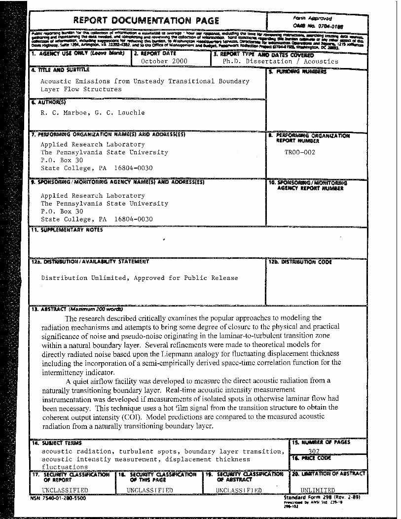
The research described critically examines the popular approaches to modeling the radiation mechanisms and attempts to bring some degree of closure to the physical and practical significance of noise and pseudo-noise originating in the laminar-to-turbulent transition zone within a natural boundary layer. Several refinements were made to theoretical models for directly radiated noise based upon the Liepmann analogy for fluctuating displacement thickness including the incorporation of a semi-empirically derived space-time correlation function for the intermittency indicator.
A quiet airflow facility was developed to measure the direct acoustic radiation from a naturally transitioning boundary layer. Real-time acoustic intensity measurement instrumentation was developed if measurements of isolated spots in otherwise laminar flow had been necessary. This technique uses a hot film signal from the transition structure to obtain the coherent output intensity (COI). Model predictions are compared to the measured acoustic radiation from a naturally transitioning boundary layer.
1«. SUftJICT TIMM
acoustic radiation, turbulent spots, boundary layer transition, acoustic intenstiy measurement, displacement thickness fluctuations
17. SECURITY OASSJfJCATIO« OF REPORT
UNCLASSIFIED
Ig. SECURITY OASSSHCATiOfä OP THIS PASS
UNCLASSIFIED
19. SSCUWTY OASSStCABOSI Of ASSTRAC?
UNCLASSIFIED
IS. NUMSSfg Of PAGES
302 is. pwcicese
29. UMTTATfON Of ASSTHACT
UNLIMITED NSN 75*MM-280-5500 Standard Form 298 (R@v 2-89)
Pmcnted b» AN« «d. l39-<t
ABSTRACT
The true acoustic radiation contribution of boundary layer flow structures has
been the subject of debate for many years. The research described here critically
examines the popular approaches to modeling the radiation mechanisms and attempts to
bring some degree of closure to the physical and practical significance of noise and
pseudo-noise originating in the laminar-to-turbulent transition zone within a natural
boundary layer. This includes improving models to include recent computational and
experimental statistics, an evaluation of model sensitivities to input parameters, and the
applicability significance for situations of engineering relevance.
There have been significant efforts over the last twenty years to model the
statistics of the wall pressure fluctuations resulting from flow structures within the
laminar-to-turbulent boundary layer transition zone. Models for the directly radiated
noise from these structures have, in turn, depended upon these statistics. Measurements
of the space-time statistics for these pressures allow further development of prediction
codes. Several refinements have been made to a theoretical model for the directly
radiated noise based upon the Liepmann analogy for fluctuating displacement thickness
including the incorporation of a semi-empirically derived space-time correlation function
for the intermittency indicator and a dipole source description for the induced wall normal
velocity. A similar model exists consisting of a Lighthill acoustic analogy using a two-
fluids model. An additional model for radiation by vortex structures within the transition
zone is qualitatively reviewed. The predominant effort in the last eight years has been to
iii
apply direct numerical simulation methods to solving for acoustic radiation. These efforts
are reviewed to help define their useful role in predicting sound radiation from transition.
The role of pressure gradient in axisymmetric body flows, flat plate flows, and over air-
and hydrofoils is investigated for incorporation into the model through a sensitivity
analysis on affected flow parameters.
A quiet airflow facility was developed and refined to measure the direct acoustic
radiation from a naturally transitioning boundary layer using time-averaged acoustic
intensity. Real-time acoustic intensity measurement instrumentation was developed in
case measurements of isolated turbulent spots in otherwise laminar flow had been
necessary. This technique uses a hot film signal from the transition structure to obtain the
coherent output intensity (COI).
Comparisons are made of model predictions to the measured acoustic radiation
from a naturally transitioning boundary layer. Radiated noise measurements isolating the
direct radiation from a transition zone demonstrated similar dependence with axial
location within the transition zone as previous wall pressure measurements. This
included radiated noise levels near mid transition zone that were higher than the noise
level produced by a fully turbulent boundary layer by 2-3 dB. The levels measured
suggest that the radiation from transition flow structures is multipolar and has a higher
radiation efficiency than the quadrupole TBL sources. Transition noise per unit area is
greater than TBL noise per unit area. Thus, the contribution to overall directly radiated
flow noise from the transition zone in typical engineering applications is negligible
compared to the radiation from the much larger area of fully turbulent flow.
IV
TABLE OF CONTENTS
Page
LISTOFFIGURES x
LIST OFTABLES xix
LIST OF SYMBOLS xx
ACKNOWLEDGMENTS xxii
CHAPTER 1 INTRODUCTION 1
1.1 Background 1
1.2 Boundary Layer Transitional Flows 2 1.2.1 Boundary Layer Flow Structures 3 1.2.2 Transitional Rows 3
1.3 Goals and Scope of the Present Investigation 6
CHAPTER 2 MODELS FOR BOUNDARY LAYER TRANSITION ZONE ACOUSTIC RADIATION 16
2.1 Fluctuating Shear Stress Using a Lighthill Analogy 17
2.2 Fluctuating Boundary Layer Displacement Thickness Using a Liepmann Analogy 20 2.2.1 Formulation Based on Lauchle Theoretical Space-Time
Correlation Function 20 2.2.2 Formulation Based on Josserand-Lauchle Measured
Space-Time Correlation Function 22 2.2.3 Chase Statistical Modification 23
2.3 Two Fluids Model Using a Lighthill Analogy 24
2.4 Vortex Motions 27
2.5 Direct Numerical Simulation 28
TABLE OF CONTENTS (continued)
Page 2.6 Direct and Indirect Radiation from Complex Geometries 32
2.6.1 Vicinity of Half-Plane Leading Edge 32 2.6.2 Bodies of Revolution 35 2.6.3 Airfoils and Hydrofoils 37
2.7 Need for Refining the Fluctuating Boundary Layer Displacement Thickness Model in a Natural Transition Region 38 2.7.1 Example Applications of Fluctuating Displacement
Thickness Model 41 2.7.2 Study Objectives: Acoustic Emissions from Isolated
Transition Flow Structures and Natural Transition Zone.. 42
CHAPTER 3 MODEL REFINEMENTS 55
3.1 Fluctuating Boundary Layer Displacement Thickness Using a Liepmann Analogy - Theoretical Space-Time Correlation Function 56 3.1.1 Computational Model Refinements 57 3.1.2 Incorporation of Measured Normal Velocity Fluctuations . 61
3.2 Fluctuating Boundary Layer Displacement Thickness Using a Liepmann Analogy - Empirical Space-Time Correlation Function 63 3.2.1 Integration of Josserand-Lauchle Correlation Function ... 63 3.2.2 Chase Statistical Modification 65
3.3 Two Fluids Model with Refined Normal Velocity 66
3.4 Accounting for Vortical Motion 66
3.5 Incorporation of Green's Function for Transition Zone Near Half-Plane Leading Edge 68
CHAPTER 4 RADIATED SOUND POWER PREDICTIONS 80
4.1 Model Comparisons 80 4.1.1 Comparisons of Models for Air Flows 82 4.1.2 Comparisons of Models for Water Flows 83
VI
TABLE OF CONTENTS (continued)
Page 4.2 Role of Rise Time, t, 83
4.3 Effects of Pressure Gradient 84
4.4 Effects of Scattering by a Plane Leading Edge 86
4.5 General Assessment of Models 86
CHAPTER 5 EXPERIMENTAL APPARATUS 103
5.1 Quiet Airflow Facility 104 5.1.1 Flow-Through Anechoic Chamber 104 5.1.2 Air Source 105 5.1.3 Flow Management 107 5.1.4 Test Section 108 5.1.5 Half-Plane 109 5.1.6 Diffuser 110
5.2 Instrumentation and Signal Processing Ill 5.2.1 Hot Wire Anemometry Ill 5.2.2 Sound Pressure 115 5.2.3 Acoustic Intensity 116 5.2.4 Coherent Output Intensity 119 5.2.5 Other Processing Hardware and Software 120
CHAPTER 6 MEASUREMENT RESULTS 142
6.1 Test Section Row 142
6.2 Intensity Measurement Calibration 143
6.3 Flat Plate Natural Transition Zone 145
CHAPTER 7 CONCLUSIONS AND FUTURE WORK 179
7.1 Conclusions 179
7.2 General Observations on Transition Noise 180
7.3 Recommended Future Work 183
Vll
TABLE OF CONTENTS (continued)
Page BIBLIOGRAPHY 185
APPENDIX A MATHCAD MODEL FILES 201
A.l Fluctuating Shear Stress Using a Lighthill Analogy 202
A.2 Fluctuating Boundary Layer Displacement Thickness Using a Liepmann Analogy - Theoretical Space-Time Correlation Function 212
A.3 Fluctuating Boundary Layer Displacement Thickness Using a Liepmann Analogy - Theoretical Space-Time Correlation Function with Krane Dipole Source Model 222
A.4 Fluctuating Boundary Layer Displacement Thickness Using a Liepmann Analogy - Empirical Space-Time Correlation Function 234
A.5 Noise Generated by Boundary Layer Transition on Symmetric Hydrofoils - Howe Formulation 240
A.6 Calculation of Boundary Layer Descriptors - Air 253
A.7 Calculation of Boundary Layer Descriptors - Water 258
A.8 Calculation of Nozzle Contours 263
A.9 Calculation of Measurement Errors from a Two Microphone Intensity Probe 268
APPENDIX B QUIET AIRFLOW FACILITY DEVELOPMENT 271
B.l Power Source Improvements 271
B.2 Blower Noise Improvements 272
B.3 Noise Reduction at the Test Plate 273
B.4 Relocation of Test Section and New Nozzle Design .... 275
Vlll

TABLE OF CONTENTS (continued)
Page B.5 Diffuser Design 276
APPENDK C REAL-TIME ACOUSTIC INTENSITY SIGNAL PROCESSING 288
C.l Time-Averaged Intensity Processing 289
C.2 Real-Time Intensity Processing 289
C.3 Conditioning with a Shear Stress Sensor 291
IX
LIST OF FIGURES
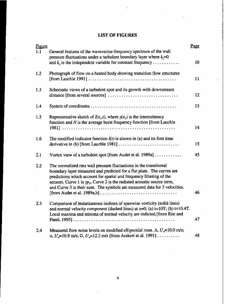
Figure Page 1.1 General features of the wavevector-frequency spectrum of the wall
pressure fluctuations under a turbulent boundary layer where ^=0 and kx is the independent variable for constant frequency 10
1.2 Photograph of flow on a heated body showing transition flow structures [from Lauchle 1991] 11
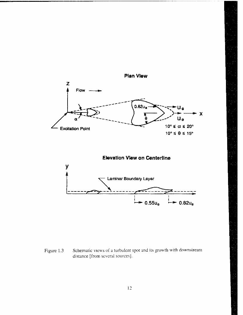
1.3 Schematic views of a turbulent spot and its growth with downstream distance [from several sources] 12
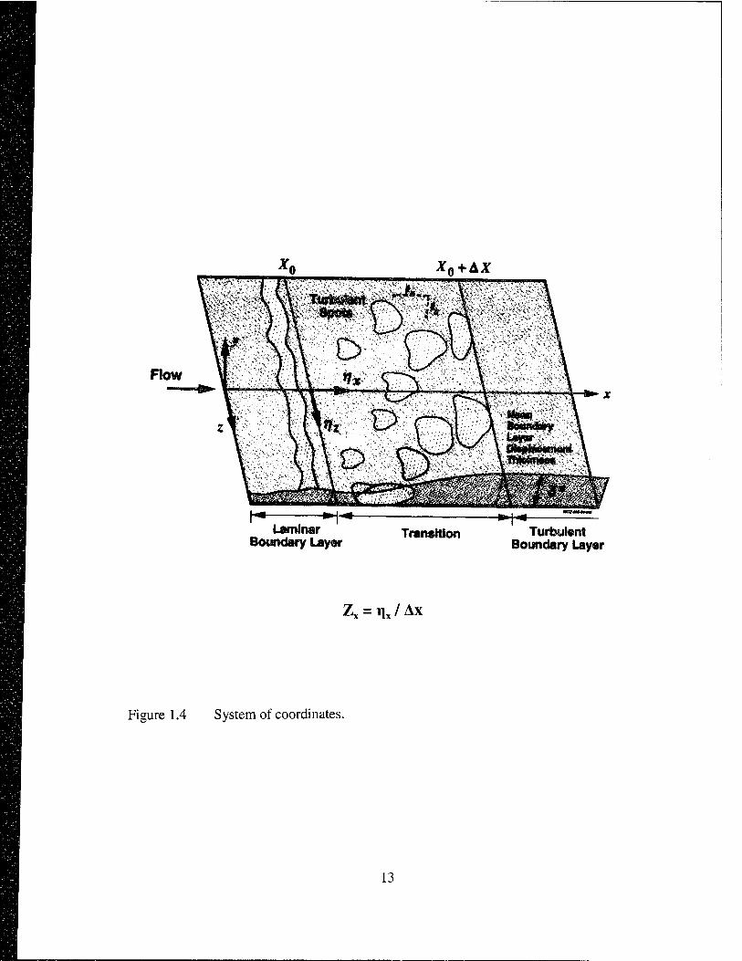
1.4 System of coordinates 13
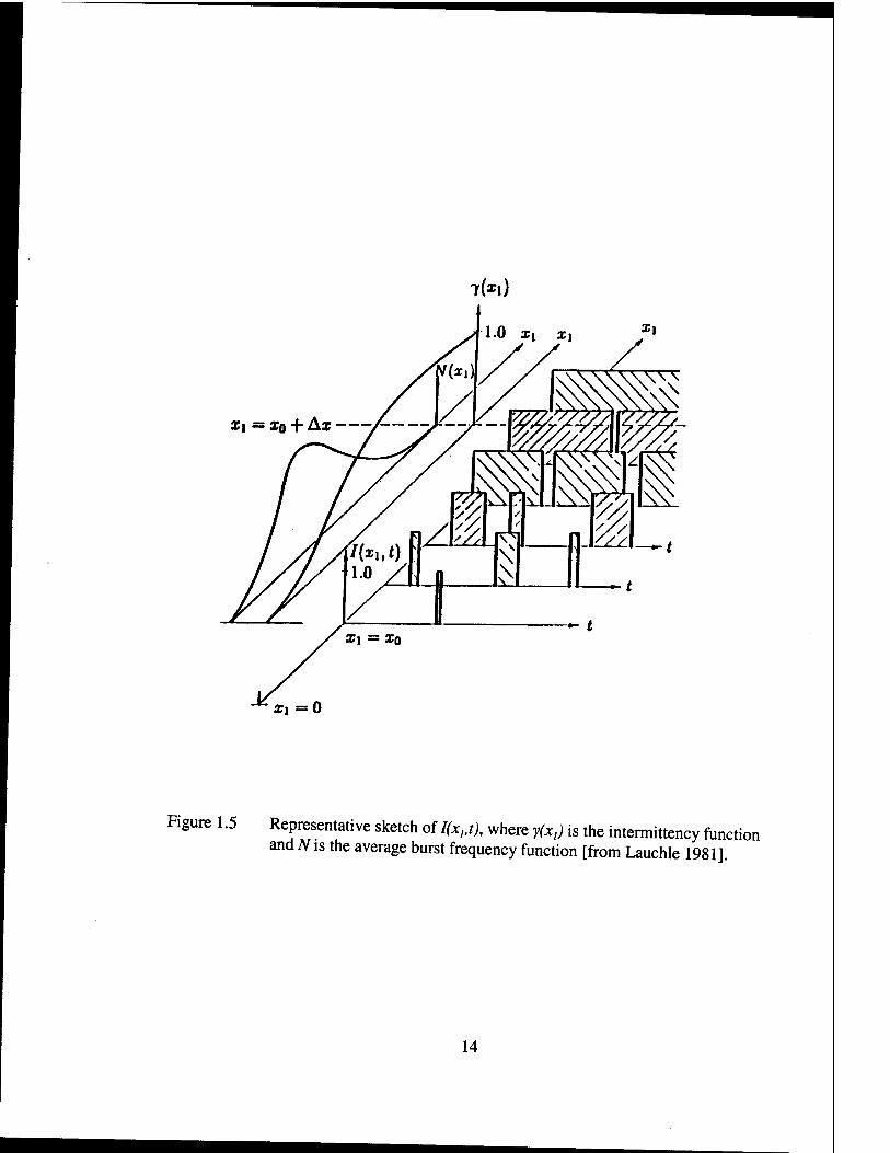
1.5 Representative sketch of I(xltt), where y(x,) is the intermittency function and N is the average burst frequency function [from Lauchle 1981] 14
1.6 The modified indicator function I(t) is shown in (a) and its first time derivative in (b) [from Lauchle 1981] 15
2.1 Vortex view of a turbulent spot [from Audet et al. 1989a] 45
2.2 The normalized rms wall pressure fluctuations in the transitional boundary layer measured and predicted for a flat plate. The curves are predictions which account for spatial and frequency filtering of the sensors. Curve 1 is yp-r, Curve 2 is the radiated acoustic source term, and Curve 3 is their sum. The symbols are measured data for 3 velocities. [from Audet et al. 1989a,b] 46
2.3 Comparison of instantaneous isolines of spanwise vorticity (solid lines) and normal velocity component (dashed lines) at z=0: (a) t=10T; (b) t=10.4T. Local maxima and minima of normal velocity are indicted, [from Rist and Fasel, 1995] 47
2.4 Measured flow noise levels on modified ellipsoidal nose. A, Uj=l0.0 m/s; o, U=10.9 m/s; □, U=12.2 m/s [from Arakeri et al. 1991] 48
LIST OF FIGURES (continued)
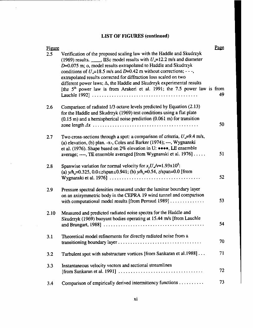
Figure Page 2.5 Verification of the proposed scaling law with the Haddle and Skudrzyk
(1969) results. , IISc model results with U=\2.2 m/s and diameter D=0.075 m; o, model results extrapolated to Haddle and Skudrzyk conditions of Uj=lS.5 m/s and D=0.42 m without corrections; —, extrapolated results corrected for diffraction loss scaled on two different power laws; A, the Haddle and Skudrzyk experimental results [the 5th power law is from Arakeri et al. 1991; the 7.5 power law is from Lauchle 1992] 49
2.6 Comparison of radiated 1/3 octave levels predicted by Equation (2.13) for the Haddle and Skudrzyk (1969) test conditions using a flat plate (0.15 m) and a hemispherical noise prediction (0.061 m) for transition zone length Ax 50
2.7 Two cross-sections through a spot: a comparison of criteria, Um=9A m/s, (a) elevation, (b) plan, -x-, Coles and Barker (1974); —, Wygnanski et al. (1976). Shape based on 2% elevation in U: ••••, LE ensemble average; —, TE ensemble averaged [from Wygnanski et al. 1976] 51
2.8 Spanwise variation for normal velocity for xsUJv=\.93x 105: (a) y/h =0.325,0.0sz/spans0.941; (b) y/h =0.54, z/span=0.0 [from Wygnanski et al. 1976] 52
2.9 Pressure spectral densities measured under the laminar boundary layer on an axisymmetric body in the CEPRA 19 wind tunnel and comparison with computational model results [from Perraud 1989] 53
2.10 Measured and predicted radiated noise spectra for the Haddle and Skudrzyk (1969) buoyant bodies operating at 15.44 m/s [from Lauchle and Brungart, 1988] 54
3.1 Theoretical model refinements for directly radiated noise from a transitioning boundary layer 70
3.2 Turbulent spot with substructure vortices [from Sankaran et al.1988]... 71
3.3 Instantaneous velocity vectors and sectional streamlines [from Sankaran et al. 1991] 72
3.4 Comparison of empirically derived intermittency functions 73
XI
LIST OF FIGURES (continued)
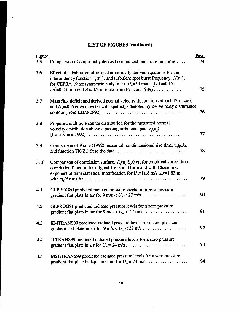
Figure Page 3.5 Comparison of empirically derived normalized burst rate functions .... 74
3.6 Effect of substitution of refined empirically derived equations for the intermittency function, y(\), and turbulent spot burst frequency, N(t\x), for CEPRA 19 axisymmetric body in air, Uj=50 m/s, uct/Jjc=0.15, AS*=0.25 mm and Ax=0.2 m (data from Perraud 1989) 75
3.7 Mass flux deficit and derived normal velocity fluctuations at x=l. 13m, z=0, and Uj=40.6 cm/s in water with spot edge denoted by 2% velocity disturbance contour [from Krane 1992] 76
3.8 Proposed multipole source distribution for the measured normal velocity distribution above a passing turbulent spot, V^T^) [from Krane 1992] 77
3.9 Comparison of Krane (1992) measured nondimensional rise time, uctJAx, and function TK(ZJ fit to the data 78
3.10 Comparison of correlation surface, Rft\x£x,0,x), for empirical space-time correlation function for original Josserand form and with Chase first exponential term statistical modification for £/j=11.8 m/s, Ax=l.S3 m, with r]JAx = 0.50 79
4.1 GLPROG80 predicted radiated pressure levels for a zero pressure gradient flat plate in air for 9 m/s <U„<21 m/s 90
4.2 GLPROG81 predicted radiated pressure levels for a zero pressure gradient flat plate in air for 9 m/s < £/„ < 27 m/s 91
4.3 KMTRANS00 predicted radiated pressure levels for a zero pressure gradient flat plate in air for 9 m/s < f/„ < 27 m/s 92
4.4 JLTRANS99 predicted radiated pressure levels for a zero pressure gradient flat plate in air for U„ = 24 m/s 93
4.5 MSHTRANS99 predicted radiated pressure levels for a zero pressure gradient flat plate half-plane in air for U„ = 24 m/s 94
Xll
LIST OF FIGURES (continued)
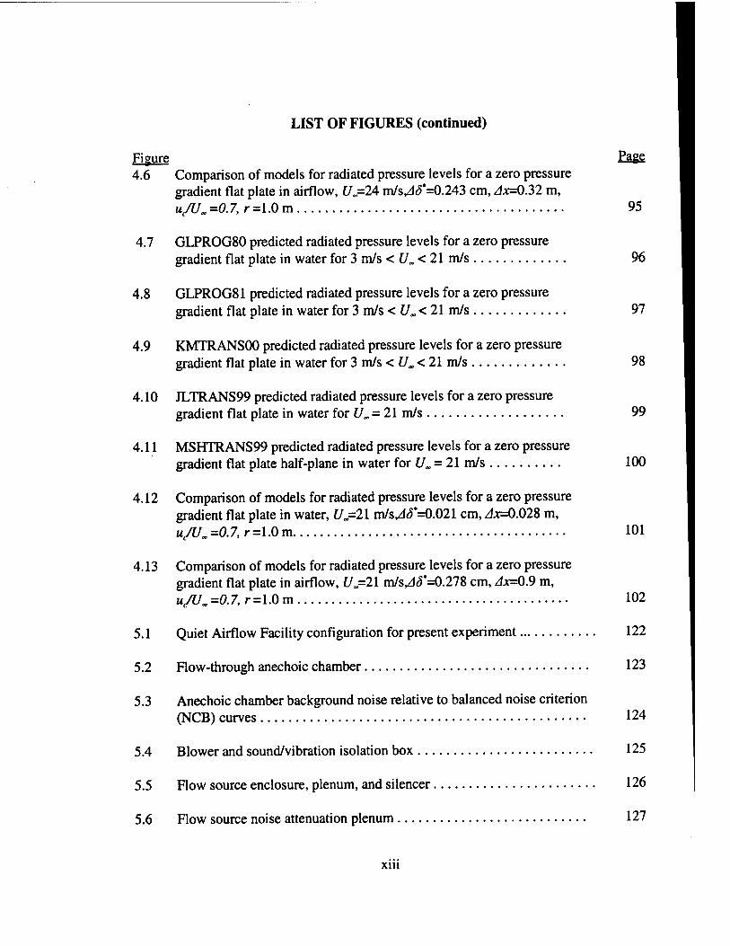
Figure Page 4.6 Comparison of models for radiated pressure levels for a zero pressure
gradient flat plate in airflow, U=24 m/syd(5*=0.243 cm, zlx=0.32 m, uJUm =0.7, r =1.0 m 95
4.7 GLPROG80 predicted radiated pressure levels for a zero pressure gradient flat plate in water for 3 m/s < £/„ < 21 m/s 96
4.8 GLPROG81 predicted radiated pressure levels for a zero pressure gradient flat plate in water for 3 m/s < (/„ < 21 m/s 97
4.9 KMTRANS00 predicted radiated pressure levels for a zero pressure gradient flat plate in water for 3 m/s < U„ < 21 m/s 98
4.10 JLTRANS99 predicted radiated pressure levels for a zero pressure gradient flat plate in water for U„ = 21 m/s 99
4.11 MSHTRANS99 predicted radiated pressure levels for a zero pressure gradient flat plate half-plane in water for U„ = 21 m/s 100
4.12 Comparison of models for radiated pressure levels for a zero pressure gradient flat plate in water, U=2l m/s<dö'=0.021 cm, Ax=O.02S m, u/U„=0J, r=1.0m 101
4.13 Comparison of models for radiated pressure levels for a zero pressure gradient flat plate in airflow, U=2l m/s,zf<5*=0.278 cm, Ax=Q.9 m, u/U„ =0.7, r =1.0 m 102
5.1 Quiet Airflow Facility configuration for present experiment 122
5.2 Flow-through anechoic chamber 123
5.3 Anechoic chamber background noise relative to balanced noise criterion (NCB) curves 124
5.4 Blower and sound/vibration isolation box 125
5.5 Flow source enclosure, plenum, and silencer 126
5.6 Flow source noise attenuation plenum 127
xni
LIST OF FIGURES (continued)
Figure Page 5.7 Buffalo Forge blower and motor 128
5.8 Elbow and conduit pipe for flow into anechoic chamber 129
5.9 In-flow silencer and diffuser into acoustic settling chamber 130
5.10 Row management plenum, diffuser, screens and settling sections prior to nozzle 131
5.11 New nozzle contracting to 15.2 cm x 30.5 cm 132
5.12 View of test section 133
5.13 Test section view showing drilled holes for hot film probe or spot generation excitation 134
5.14 View of nozzle, plenum, and diffuser 135
5.15 Stethoscope burst probe 136
5.16 Half-plane plate designed for test section 137
5.17 Looking upstream through diffuser to the test section and the added diffuser resistance 138
5.18 Intensity probe calibration tubes, (a) high frequency and (b) low frequency 139
5.19 Processing diagram for coherent output intensity 140
5.20 Anemometer and microphone amplifier 141
5.21 Test instrumentation 141
6.1 Boundary layer profile for U = 23.1 m/s, x =7.6 cm, y=2.54 cm from centerline 149
6.2 Spanwise uniformity of the test section streamwise velocity for U=23.1 m/s, x = 7.6 cm, at 25,50, and 75% of test section height... 150
xiv
LIST OF FIGURES (continued)
Figure Page 6.3 Spanwise uniformity of the test section streamwise velocity for
U=23.1 m/s, x = 77.5 cm, at 25, 50, and 75% of test section height... 151
6.4 Comparison of boundary layer profiles and turbulence intensity profiles tripped, fully turbulent flow for nominal U=23.9 m/s near end of test section 152
6.5 Calibration configuration 153
6.6 Magnitude and phase of microphone mismatch as measured in small calibration tube 154
6.7 Intensity estimate bias errors due to point monopole and dipole source fields for microphone separation of 2.54 cm 155
6.8 Comparison of (a) P-P time-averaged intensity measurement to far field intensity at 0.8m above speaker, and (b) P-P time-averaged intensity measurement with and without mylar to open far field intensity at 0.5m above speaker in 1.6 Hz bands 156
6.9 Comparison of P-P time-averaged intensity measurement with and without mylar to open far field intensity at 0.5m above speaker in (a) 50 Hz bands and (b) 1/3 octave bands 157
6.10 Intensity probe gain over a single microphone 158
6.11 Configuration of P-P intensity probe for transition zone measurements 159
6.12 Locations and levels of hot film measurements for intermittency compared to Josserand intermittency function and locations of intensity measurements 160
6.13 Examples of spectrum smoothing achieved through wider band processing 161
6.14 Active intensity in 1.6 and 50 Hz processing bands measured for natural transition region of 21 m/s in zero pressure gradient above mylar wall for -0.03< Z, < 0.60 162
xv
Figure 6.15
LIST OF FIGURES (continued)
Active intensity in 1.6 and 50 Hz processing bands measured for natural transition region of 21 m/s in zero pressure gradient above mylar wall for Z - -0.03,0.45 and 0.53 259
Page
163
164
165
166
167
168
169
170
171
172
6.16 Boundary layer trip of 50 grit sandpaper in 6 cm long strip at x= 20 cm and boundary layer stimulation of 150 grit sandpaper in two 10mm long strips at x= 12 and 15 cm
6.17 Active intensity in 1.6 and 50 Hz processing bands measured for tripped turbulent flow at 21 m/s in zero pressure gradient above mylar wall for -0.03< Z < 0.60
6.18 Active intensity in 1.6 and 50 Hz processing bands measured for tripped turbulent flow at 21 m/s in zero pressure gradient above mylar wall for Z - -0.03,0.45 and 0.53
6.19 Active intensity in 1.6 and 50 Hz processing bands measured for stimulated transition region at 21 m/s in zero pressure gradient above mylar wall for -0.03< Z < 0.60
6.20 Active intensity in 1.6 and 50 Hz processing bands measured for stimulated transition region at 21 m/s in zero pressure gradient above mylar wall for Z - -0.03,0.45 and 0.53
6.21 Comparison of active intensity in 1.6 and 50 Hz processing bands measured for natural and stimulated transition and tripped turbulent flow at 21 m/s in zero pressure gradient above mylar wall for Zx = -0.03
6.22 Comparison of active intensity in 1.6 and 50 Hz processing bands measured for natural and stimulated transition and tripped turbulent flow at 21 m/s in zero Dressure gradient above mvlar wall for Z = 0.09
6.23 Comparison of active intensity in 1.6 and 50 Hz processing bands measured for natural and stimulated transition and tripped turbulent flow at 21 m/s in zero Dressure gradient above mvlar wall for Z, = 0.20
6.24 Comparison of active intensity in 1.6 and 50 Hz processing bands measured for natural and stimulated transition and tripped turbulent flow at 21 m/s in zero nressure gradient above mvlar wall for Z. — 0.31
xvi
LIST OF FIGURES (continued)
Figure Page 6.25 Comparison of active intensity in 1.6 and 50 Hz processing bands measured
for natural and stimulated transition and tripped turbulent flow at 21 m/s in zero pressure gradient above mylar wall for Zx = 0.45 173
6.26 Comparison of active intensity in 1.6 and 50 Hz processing bands measured for natural and stimulated transition and tripped turbulent flow at 21 m/s in zero pressure gradient above mylar wall for Zx = 0.53 174
6.27 Comparison of active intensity in 1.6 and 50 Hz processing bands measured for natural and stimulated transition and tripped turbulent flow at 21 m/s in zero pressure gradient above mylar wall for Zx = 0.60 175
6.28 Fluctuating wall pressure measurements made in air by Dufourq (1984). 176
6.29 Comparison of transition noise model predictions with measured directly radiated sound pressure levels 177
6.30 Comparison of intermittency weighted measured turbulent boundary layer noise with measured transition zone directly radiated sound pressure levels 178
B. 1 Original orientation of Quiet Airflow Facility to the flow-through anechoic chamber 278
B.2 Comparison of narrowband signature of Borg-Warner inverter and replacement ABB inverter for (a) upstream plenum and (b) airborne levels in control room 279
B.3 Original semi-circular wall jet over flat plate configuration 280
B.4 Addition of suction manifold below test plate 281
B.5 Views of suction manifold ports and rods with cones 282
B.6 Measured sound pressure level for assembly in control room running at Uj=ll.S m/s compared to GLPROG81 predictions for uctj/zlx=0.15 and uAJAx=0.05 283 -C"T
B.7 GLPROG81 sound pressure level predictions for U=\ 1.8 m/s and several uciJAx values otherwise matching Figure B.6 284
xvii
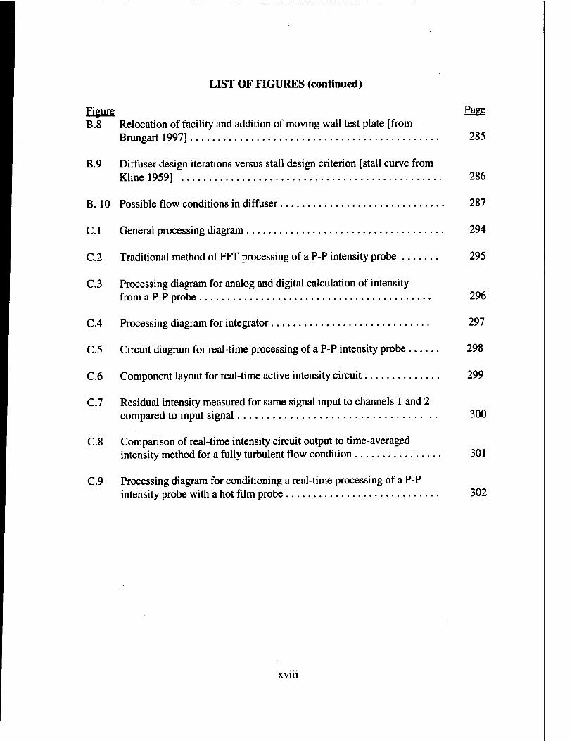
LIST OF FIGURES (continued)
Figure Page B.8 Relocation of facility and addition of moving wall test plate [from
Brungart 1997] 285
B.9 Diffuser design iterations versus stall design criterion [stall curve from Kline 1959] 286
B. 10 Possible flow conditions in diffuser 287
C.l General processing diagram 294
C.2 Traditional method of FFT processing of a P-P intensity probe 295
C.3 Processing diagram for analog and digital calculation of intensity from a P-P probe 296
C.4 Processing diagram for integrator 297
C.5 Circuit diagram for real-time processing of a P-P intensity probe 298
C.6 Component layout for real-time active intensity circuit 299
C.7 Residual intensity measured for same signal input to channels 1 and 2 compared to input signal 300
C.8 Comparison of real-time intensity circuit output to time-averaged intensity method for a fully turbulent flow condition 301
C.9 Processing diagram for conditioning a real-time processing of a P-P intensity probe with a hot film probe 302
xvm
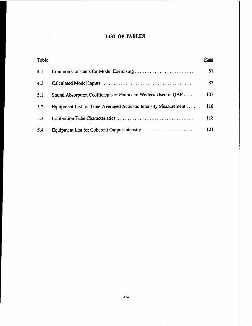
LIST OF TABLES
Table Page
4.1 Common Constants for Model Exercising 81
4.2 Calculated Model Inputs 82
5.1 Sound Absorption Coefficients of Foam and Wedges Used in QAF 107
5.2 Equipment List for Time-Averaged Acoustic Intensity Measurement 118
5.3 Calibration Tube Characteristics 118
5.4 Equipment List for Coherent Output Intensity 121
xix
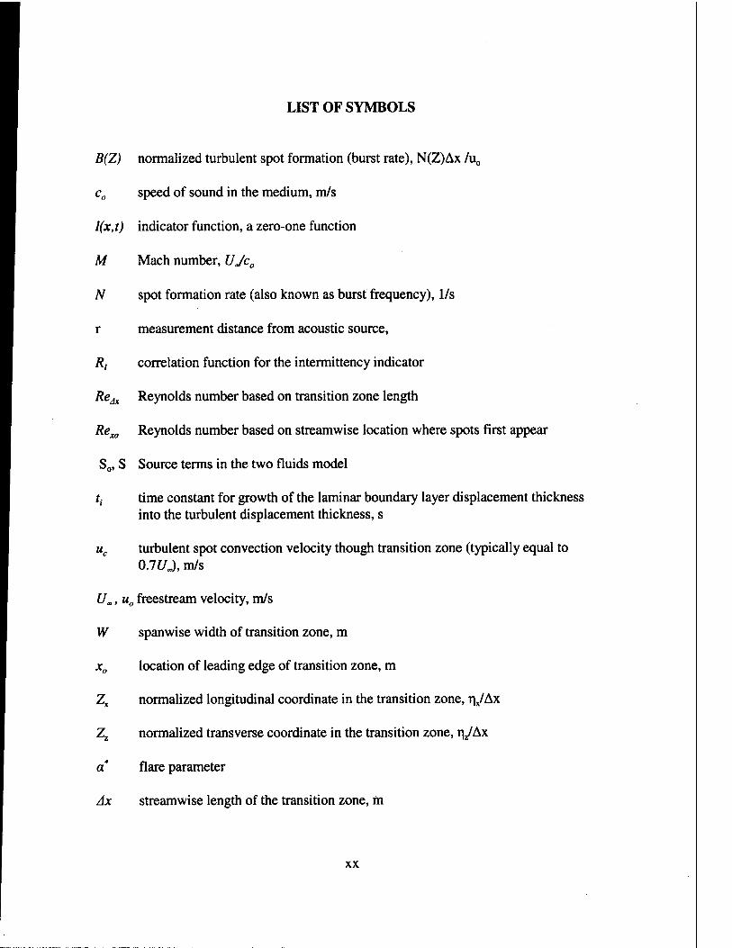
LIST OF SYMBOLS
B(Z) normalized turbulent spot formation (burst rate), N(Z)Ax /u0
c0 speed of sound in the medium, m/s
I(x,t) indicator function, a zero-one function
M Mach number, UJc0
N spot formation rate (also known as burst frequency), 1/s
r measurement distance from acoustic source,
R, correlation function for the intermittency indicator
ReM Reynolds number based on transition zone length
Rexg Reynolds number based on streamwise location where spots first appear
S0, S Source terms in the two fluids model
tt time constant for growth of the laminar boundary layer displacement thickness into the turbulent displacement thickness, s
uc turbulent spot convection velocity though transition zone (typically equal to OJUJ, m/s
U„, u0 freestream velocity, m/s
W spanwise width of transition zone, m
x0 location of leading edge of transition zone, m
Zx normalized longitudinal coordinate in the transition zone, VAx
Zz normalized transverse coordinate in the transition zone, n^Ax
a flare parameter
Ax streamwise length of the transition zone, m
xx
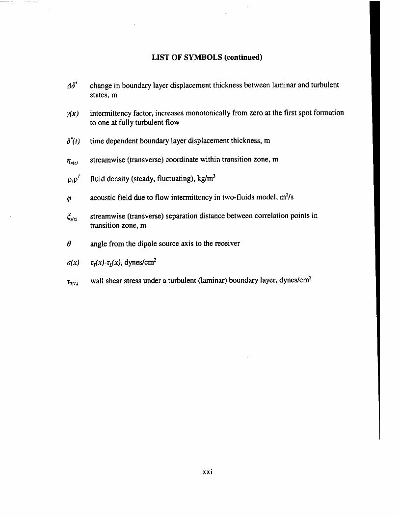
LIST OF SYMBOLS (continued)
AS* change in boundary layer displacement thickness between laminar and turbulent states, m
y(x) intermittency factor, increases monotonically from zero at the first spot formation to one at fully turbulent flow
ö*(t) time dependent boundary layer displacement thickness, m
rj4l) streamwise (transverse) coordinate within transition zone, m
p,p7 fluid density (steady, fluctuating), kg/m3
<p acoustic field due to flow intermittency in two-fluids model, m2/s
£x(z) streamwise (transverse) separation distance between correlation points in transition zone, m
6 angle from the dipole source axis to the receiver
a(x) TJ(X)-TL(X), dynes/cm2
rT(L) wall shear stress under a turbulent (laminar) boundary layer, dynes/cm2
xxi
ACKNOWLEDGMENTS
I gratefully acknowledge the mentoring, support, and patience of my advisor, Prof. G. C. Lauchle as well as the contributions of my other committee members, Prof. G. H. Koopmann, Prof. D. K. McLaughlin and Prof. F. S. Archibald. I am also appreciative of the opportunity to work with Prof. M. S. Howe during his sabbatical period at Penn State.
I am also indebted to faculty and staff colleagues at the Applied Research Laboratory for their support throughout this research effort. In particular, Bob Grove provided superb construction support over the development lifetime of the Quiet Airflow Facility. Eric Riggs provided hot wire anemometry support. I am also thankful for the long standing collaboration in aeroacoustic problems with Dr. Tim Brungart.
My family has both sustained and distracted me throughout this long process, but I wouldn't have it any other way. So this work is dedicated to my wife, Rose, children, Teresa and Paul, and my parents, Robert and Evelyn Marboe.
Portions of this work were supported by a grant from the Office of Naval Research, Code 1125 OA and the Fundamental Research Initiatives Program at the Applied Research Laboratory managed by Dr. R. Stern.
xxii
CHAPTER 1
INTRODUCTION
1.1 Background
Much debate exists over the true acoustic radiation contribution of boundary layer
flow structures. Is the near- and far-field noise significant? Current knowledge is based
on analytical theories and a very limited database of measured data where it is believed
that transition noise exists. Unfortunately, much of the data from these measurements are
questionable due to possibility of contamination by other noise sources. It seems that
sonar self-noise is affected by transition and that a radiation noise field exists, but a
refined theoretical or computational model and subsequent experimental verification is
required.
The research described in this dissertation critically examines the popular
approaches to modeling the radiation mechanisms and brings a degree of closure to the
physical and practical significance of noise and pseudo-noise originating in the laminar-
to-turbulent transition zone within a natural boundary layer. This effort includes updating
of models to include computational and experimental statistics plus an evaluation of
model sensitivities, applicability, and significance for situations of engineering relevance.
There have been significant efforts over the last twenty years to model the wall
pressures resulting from flow structures within the laminar-to-turbulent boundary layer
transition zone. Knowledge of the wavevector-frequency spectrum of the wall pressures

can be used to predict indirect radiation from excitation of the structure over which
transition occurs.
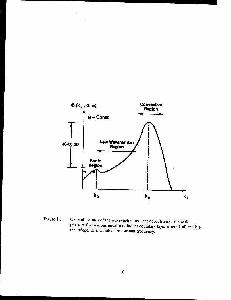
Josserand and Lauchle (1990) showed that the transition zone wall pressure
fluctuation wavevector-frequency spectrum, near the convective wavenumber domain, is
equal to the wavevector-frequency spectrum for wall pressure fluctuations under a fully
turbulent boundary layer (Figure 1.1) multiplied by an intermittency factor, y. This factor
varies monotonically from zero at the beginning of transition to unity for the fully
turbulent boundary layer. The transition zone wavevector-frequency spectrum is:
Kans^AA^) = Yftx) OnA-V»)- (1.1)
Here, k=(x-x0)/Ax and the function &TBL used by Josserand and Lauchle (1990) was
developed by Chase (1980). However, this equation is not valid over the low
wavenumber or sonic region. It is thus the intent of this dissertation to refine equation
(1.1) with emphasis on the prediction of the direct radiation from transition flow
structures at sonic and supersonic wavenumbers.
1.2 Boundary Layer Transitional Flows
Since the scope of this dissertation is limited to the modeling of direct radiation
from the transition zone, it is best to refrain from detailing all of the fundamental work
that has been done to determine the fluid mechanics of transition mechanisms and the
measurements of turbulent flow structures which form the basis for the described models.
The reader is directed to the review articles of Tani (1969), Gad-el-Hak (1989), and

Lauchle (1991). Some of the more important prior developments relevant to the present
research will be discussed briefly in the next two sections.
1.2.1 Boundary Layer Flow Structures
Much of the modeling of flow structures in the transitional boundary layer has
been based on the modeling of flow structures found in the fully developed turbulent
boundary layer (TBL). The characterization of these structures has come predominately
through experimental measurements, particularly from those utilizing laser doppler
velocimetry. The models are highly empirical.
The description of flow structures and characteristics within the TBL are found in
Bershadskii and Tsinobar (1994), Honkan and Andreopoulos (1999), Klebanoff et al.
(1992), Koh (1993), Krogstad and Antonia (1994), Schlichting (1979), and White (1974).
Wall pressure models for the TBL are given by Corcos (1963), Chase (1991), Capone and
Lauchle (1995), Graham (1997), Keith and Abraham (1997), and Singer (1997). Radiated
noise models are found in Powell (1960), Chase (1987), Barker (1974), Bergeron (1973),
Howe (1998), Lauffer et al. (1964), Pierce (1981), and Tarn (1975).
1.2.2 Transitional Flows
As laminar flow over a flat or curved surface approaches a critical Reynolds
number, hydrodynamic instabilities occur. Examples are Tollmien-Schlichting, Rayleigh,
and Kelvin-Helmholtz for different flow regimes. [See Huerre and Monkewitz (1990),
Panton, (1984), Schlichting (1979), or White (1974) for more details.] For the flat plate,
two-dimensional Tollmien-Schlichting waves form in the boundary layer. These
instabilities become non-linear and three-dimensional. Bursting occurs, followed by the
formation of Emmons spots (Emmons, 1951). These spots are turbulent regions within
an otherwise laminar flow (Figures 1.2 and 1.3) which grow and coalesce to become fully
turbulent flow. The transition region, of length Ax beginning at x0, is usually defined as
the zone in which distinct Emmons spots exist.
Therefore, within this transition region, the flow can be thought of as a classical
mixture of turbulent and laminar flow zones with concentrations determined by the
intermittency function y(rjx) and l-y(rjj, respectively. Here, y(rjx) is the time average value
of I(x,t), the intermittency indicator function which has the value of zero for a laminar
state and unity for a turbulent state. The system of coordinates and relevant flow
characteristics are shown in Figure 1.4. This function is typically used for y=0. For
infinite span, we expect Ifrj^^t) to be statistically homogeneous in the rjz direction but
non-homogeneous in the r\x direction. So, the time average value will be independent of
r\z and vary from 0.0 at rj=0 to 1.0 at rj=Ax. The burst frequency, N(rjx), describes the
mean number of Emmons spots which pass a point per unit time. The general behavior of
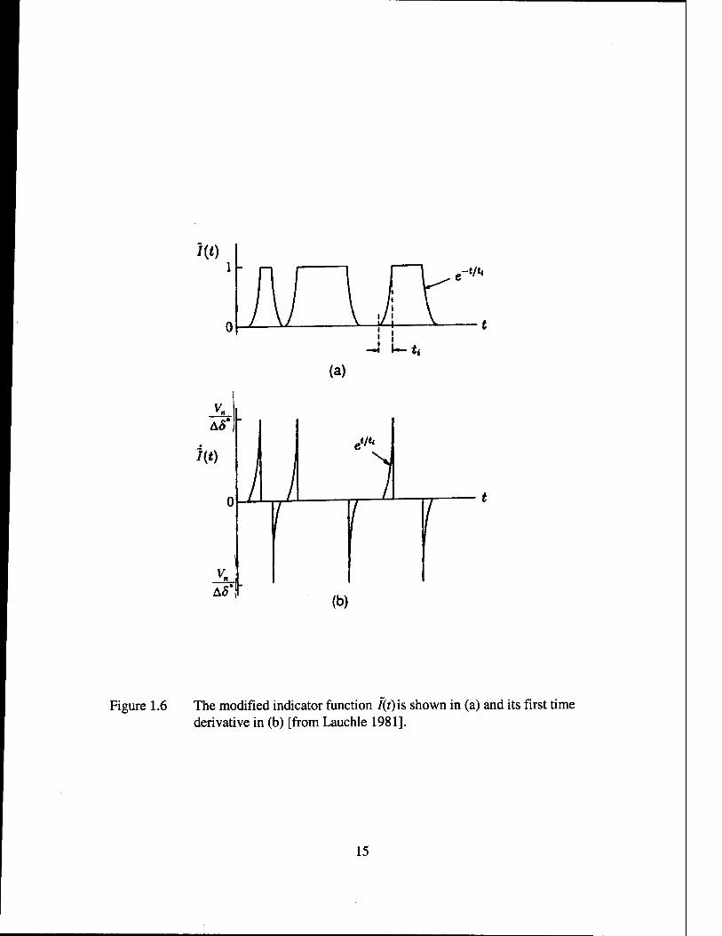
these functions through the transition zone can be seen in Figure 1.5. While the ideal
indicator function is constructed with step functions, a physically realizable indicator
includes rise times as shown in Figure 1.6. This rise time accounts for the time for the
flow to change from a laminar flow value to a turbulent flow one and conversely
(Lauchle, 1989). As shown in Figure 1.6, the rate of change of the indicator function is
described by e'"'. If this change in flow state, with inherent increase in displacement
thickness from laminar to turbulent, were considered as a piston movement, then a shorter
time, tj, would result in higher source surface velocity and a higher radiated noise. This
time should be a function of the flow velocity and other characteristics of transition zone
which are fluid dependent.
The transition zone length can be predicted from empirical formulae of the form
Re^ = C Re" (1.2)
where the Reynolds numbers are based on the subscripted length and freestream velocity,
U^ Chen and Thyson (1971) found C=60 and n=2/3 for blunt nosed bodies which
accounted for positive pressure gradients and Mach number. However, values have been
derived from the flat plate experimental data of Dhawan and Narasimha (1958): C=15
and n=0.8, and from Josserand and Lauchle (1990): C=17 and n=0.8. Narasimha et al.
(1984) argued that, because the spots do not propagate at consistent speeds proportional
to freestream velocity, every pressure gradient results in a unique intermittency
distribution, and Equation (1.2) must be adjusted accordingly.
Once again, there have been many investigations covering transition mechanisms
and flow structures described in the literature. The following are some representative
references that were found to be helpful. Modeling of transition mechanisms is described
by Barenblatt (1990), Gogineni. and Shih (1997), and Stewart and Smith (1992).
Definitions of the characteristics of turbulent spots themselves can be found in
Barrow et al. (1984), Gad-el-Hak and Fazle Hussain (1986), Henningson and Alfredsson
(1987), Jahanmari et al. (1996), and Van Atta et al. (1982). A description of vortices in

spots is available in Haidari and Smith (1994). Details on spot intermittency through the
transition zone is provided by DeMetz and Casarella (1973), Farabee et al. (1974), Krane
(1992), Krane and Pauley (1992), Narasimha (1957), Schneider (1995), and Zhang et al.
(1995). The wall pressures resulting from turbulent spot formation, growth, and
convection are well documented in Bowles and Smith (1995), Ching and LaGraff (1995),
Gedney (1979), Gedney and Leehey (1989), Josserand and Lauchle (1989), and Mautner
(1982). Studies on the interaction of turbulent spots are given by Chemy and Pauley
(1994), and Coles and Savas (1979). The growth and convection of turbulent spots
varies with the pressure gradient over the transition zone. Several investigations have
addressed the variations with both favorable and adverse pressure gradients. These
include Bandyopadhyay and Ahmed (1993), Blair (1992 a,b), Clark et al. (1996), Dey
and Narasimha (1991), Jeon and Kang (1995), Katz et al. (1990a,b), Ramesh et al.
(1996), Seifert and Wygnanski (1995), and Walker and Gostelow (1990).
1.3 Goals and Scope of the Present Investigation
This investigation was begun under a three year Office of Naval Research
Fundamental Research Initiatives Program: Hydroacoustics of Boundary Layer
Transition. The overall objective was to identify the physical mechanisms that cause
sound radiation from intermittent (particularly transitional) boundary layer flows over
rigid surfaces. Specifically this requires:
1. evaluation of existing theoretical and semi-empirical models and new
developments or modifications based on new or refined space-time statistics;
2. experimental determination of the statistics of the unsteady fluid mechanics of
these flow structures, in particular:
- develop scalar descriptors of turbulent spot growth,
- measure space-time development of transition zone fluctuating
displacement thickness (for individual and multiple interacting spots),
- relate spot growth descriptors to sound production including the
characteristic time constants associated with the acoustic radiation
model;
3. obtain unambiguous measurements of the acoustic emissions from isolated
boundary layer flow structures including natural transition and/or individual
turbulent spots; and
4. use the existing experimental database to validate the theoretical and
semi-empirical models.
The second goal was the basis for an associated investigation which is reported in
the Ph.D. dissertation by Krane (1992) and complements the measurements by Josserand
(1986). The first, third, and fourth items were the basis for the present investigation. If
this research were viewed from a verification and validation process (Coleman and
Steele, 1999) perspective, the models have undergone verification to assure correct
implementations of equations and address computational limitations but the validation is
really more of an early evaluation of the applicability of the may models. We are still in
the discovery phase of the physical mechanisms which are contributing to the transition
zone radiated noise which has been experimentally determined for the first time.
The structure of this dissertation is as follows. Important boundary layer
parameters and definitions are covered in Chapter 1. Five approaches to modeling the
radiated noise from a transition zone are covered in Chapter 2.. These include: a
fluctuating shear stress model [Lauchle 1980], a fluctuating displacement thickness
model using the Liepmann analogy [Lauchle 1981,1989], a two-fluids model using the
Lighthill analogy [Sornette and Lagier 1984a,b, Lagier and Sornette 1986, and Audet, et
al. 1989a,b], direct numerical simulation [Wang, Lele, and Moin, 1996a], and a vortex
motions model [Kambe 1986 and Hardin 1991]. Recent activity has focused on the use
of direct numerical simulation (DNS) using full Navier-Stokes equations solvers to
predict statistical quantities relevant to a Lighthill approach. The problem statement then
evolves from examining some predictive comparisons for three test cases for which
experimental data are believed to be influenced by transition. These include a flat plate in
air, an axisymmetric body in air, and an axisymmetric body in seawater. It is apparent
that pressure gradient plays an important role in the pressure fluctuations and its effect
will also be discussed.
The computational model refinements are detailed in Chapter 3. Based on the
results of Josserand and Lauchle (1990), it is possible to make refinements to Lauchle's
(1981) model by incorporating the empirically derived space-time correlation function.
In addition, several other refinements can be made using measurements by Krane and
Pauley (1993), correlation simplifications, plus accounting for retarded time differences
and vortical motions. Predictions for several relevant flow conditions are presented in
Chapter 4.
It is important for any model to have experimental validation. The direct radiation
from transition flow structures (distinct from measured wall pressures) has not previously
been measured in isolation. Chapter 5 contains a description of the quiet airflow facility
modified for these measurements and the flow-through anechoic chamber of the Applied
Research Laboratory at The Pennsylvania State University. Acoustic intensity
instrumentation and signal processing was employed to overcome facility noise. Time-
averaged acoustic intensity measurement techniques were used successfully for the
measurements of directly radiated noise from a natural transition zone. This
measurement includes the interactions of multiple spots. These measurements are
described in Chapter 6. In anticipation of a possible need for additional noise rejection,
real-time acoustic intensity measurement instrumentation was developed. A process was
developed to use a hot film signal from the transition flow structure to obtain coherent
output intensity (COI). This technique would have been necessary for measurements of
the radiated noise from individual spots generated and convecting in otherwise laminar
flow. Conclusions and recommendations for further investigation are provided in
Chapter 7.
Mathcad ® software from Mathsoft, Inc was used for the computational modeling.
Printouts of the worksheets are provided in Appendix A. A chronology of the
development of the Quiet Airflow Facility is detailed in Appendix B. Finally, details of
the electronics developed for the real-time acoustic intensity measurement are given in
Appendix C.
<D(kx,0, <D)
r 40-60 dB
1
Conv*ctiv« Region
ca - Const.
Sonic I Roglon
Low Wavonumbtr Roglon
Figure 1.1 General features of the wavevector-frequency spectrum of the wall pressure fluctuations under a turbulent boundary layer where k=0 and kx is the independent variable for constant frequency.
10
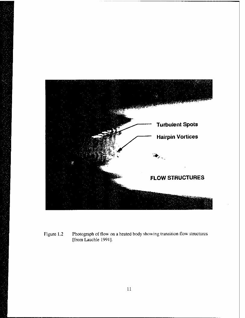
Figure 1.2 Photograph of flow on a heated body showing transition flow structures [fromLauchle 1991].
11
Plan View
a
Excitation Point
•*■ X
I0°ia$ 20°
10° S e 5S 15°
y A
Elevation View on Centerllne
Laminar Boundary Layer
-*-
0.55u« 0.82u,
Figure 1.3 Schematic views of a turbulent spot and its growth with downstream distance [from several sources].
12
Flow
r0 X0+AX II I.J.M y. 11^ I ,| || |, _ »WW— l| , L I |y || !|iij i,_ ^. ^ . ji 11 i j HI , , ^
Laminar Boundary Layar
Transition Turbulent Boundary Layer
ZX = T]X/Ax
Figure 1.4 System of coordinates.
13
7(*i)
xi = 0
Figure 1.5 Representative sketch of I(x„t), where y(x,) is the intermittency function and N is the average burst frequency function [from Lauchle 1981].
14
AS*]
/(«)
V. A5*
1
(a)
(b)
Figure 1.6 The modified indicator function I(t) is shown in (a) and its first time derivative in (b) [from Lauchle 1981].
15
CHAPTER 2
MODELS FOR BOUNDARY LAYER TRANSITION ZONE ACOUSTIC RADIATION
The modeling of flow-induced noise from boundary layer flows has been well
researched for many years. Several papers are significant and form the basis for
investigation of transition noise. The works of Lighthill (1952,1954), Ffowcs Williams
(1967,1969,1977,1982), Curie (1955), Crighton (1975), and Blake (1986), and Howe
(1998) provide a good general background.
Several approaches have been taken to model the unsteady pressures due to
boundary layer transition processes. These have predominately used the Lighthill analogy
as a basis. Lauchle (1981) took a more phenomenological approach by modeling the
displacement thickness change due to transition as a piston motion with non-uniform
velocity distribution. This was later supported through a Lighthill approach by Sornette
and Lagier (1984a). Audet et al. (1989a) then claimed the experimental appearance of
monopole-like acoustic sources. While the gross fluctuations of the growth in
displacement thickness seem to be modeled well by the piston-like sources, there is also
much interest in modeling the acoustic sources due to the vortical structures of the spots.
In this chapter, four of these models will be presented. Direct numerical simulation
efforts will be discussed briefly.
16
2.1 Fluctuating Shear Stress Using a Lighthill Analogy
Lauchle (1980) used the Lighthill acoustic analogy to find dipole, quadrupole, and
octupole components of radiated noise from transition. He assumed radiation efficiencies
scale on Mach number according to M3 and Ms for the dipole and quadrupole sources
respectively. Since a low Mach number flow was also assumed, he neglected the
quadrupoles and octupoles due to the fluctuating Reynolds stresses and their images.
However, their large amplitudes, relative to those of the wall shear stresses that form the
dipole contribution may compensate for the lower radiation efficiency and make this a
poor assumption.
The Lighthill equation for sound radiation from fluid dynamic sources is:
i2«/
dv
&J 8T„
a*.2 dxjdx. (2.1)
where Ttj is Lighthill's stress tensor given by:
T.. = pM/M.-o^ + (p/-p/cz)5,7 (2.2)
It should be noted that Fraudelplonika (2000) suggests that this stress has an additional
contribution, V(fiu), but that was not considered in the context of this development. The
tensor of Equation (2.2) consists of the fluctuating Reynolds stress tensor, p«.«;., the
fluctuating viscous shear stress tensor, a.., and a "correction" term which is essentially
zero for hydrodynamic flows.
17
Employing Curie's equation and Powell's (1960) extension for image flow with a
rigid, planar surface, Lauchle derived an estimate of the acoustic pressure due to shear
stress fluctuations only:
P(r,t) cos0 d
2 7i r c„ dt f // X° {^'L) dS^ M * l (2.3)
where 6 is the angle from the JC axis to the observation point. This, of course, assumes
that the contribution of the longitudinal and lateral quadrupoles is insignificant based on a
M ~2 reduction in radiation efficiency for low Mach number flows.
Using intermittency to model the wall shear stress in a mix of laminar and
turbulent states, dtjdt reduces to (Tr-xL) dlldt = a(x) /(JC.,/) . This results in an
equation for the power spectral density of the sound radiated per unit spanwise width of
transition:
dz 4 r r2 c„ (2.4)
This assumes that the space-time correlation function for the indicator can be separated,
the same as Corcos (1963) did for the homogeneous, fully developed turbulent boundary
layer. This requires that:
M=*M&)*MÜ. (2.5)
18
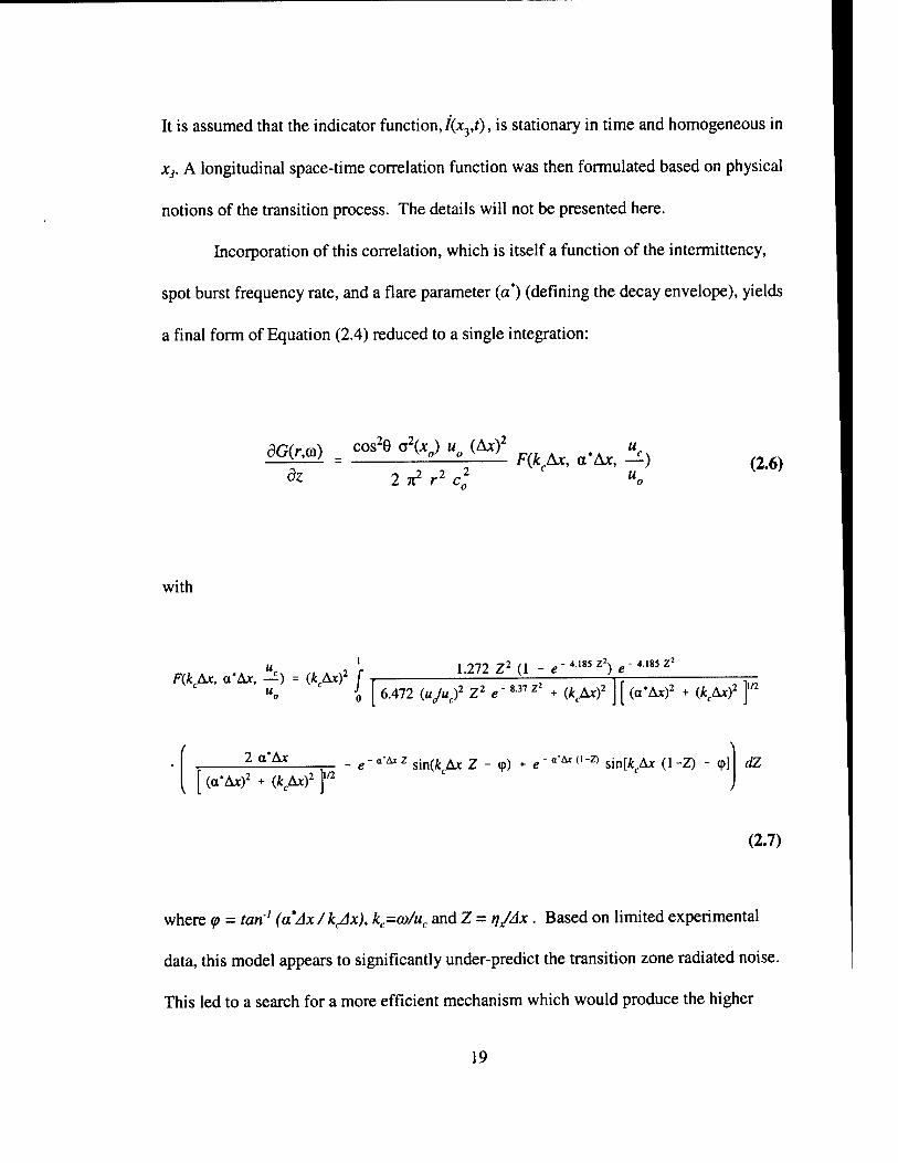
It is assumed that the indicator function,/(JC3,/), is stationary in time and homogeneous in
x3. A longitudinal space-time correlation function was then formulated based on physical
notions of the transition process. The details will not be presented here.
Incorporation of this correlation, which is itself a function of the intermittency,
spot burst frequency rate, and a flare parameter (a) (defining the decay envelope), yields
a final form of Equation (2.4) reduced to a single integration:
^) = cos*9 « ftp u. (Ax) F(k ^ o.^ u^
dz 2T?r2c2„ C uo (2.6)
with
1.272 Z2 (1 - e'*mz) e F(kAx, a*Ax, —) = (krAx)2 \ T — -y. r-
". o [ 6.472 (ujuf Z2 e"837 z' + (kcAx)2 J [ (a'Ax)2 + (kcAx)2 ]n
2 a'Ax
[ (a'Ax)2 + (kcAx)2 Y e ~ «^ z sin(* Ax Z - cp) + e-«"**<»-*> sin[*cAt (1-Z) - (pi JZ
(2.7)
where <p = ran' (aAx/k^x), kc=co/uc and Z = fl/J*. Based on limited experimental
data, this model appears to significantly under-predict the transition zone radiated noise.
This led to a search for a more efficient mechanism which would produce the higher
19
measured levels. It does not appear to be advantageous to pursue any further
modifications to this model that uses only the wall shear stresses as the source term.
2.2 Fluctuating Boundary Layer Displacement Thickness Using a Liepmann Analogy
In order to account for the previously neglected terms for the fluctuating
velocities, Lauchle (1981,1989) used the Liepmann (1954) analogy rather than calculating
the Reynolds stresses in transition as required by the Lighthill equation.
The Liepmann analogy uses the fluctuations in the boundary layer displacement
thickness to describe the normal velocity of a vibrating surface. This is the "surface" that
the potential outer flow feels as it is displaced by the boundary layer. A wave equation is
then solved for the acoustic radiation of this vibrating surface. The results of this
approach differ from LighthilFs analogy only in that the unknown source is described in
the boundary condition and not in the source terms of the Lighthill inhomogeneous wave
Equation (2.1). The use of displacement thickness fluctuations in acoustic modeling was
also recognized by Lighthill (1958) and Howe (1981).
2.2.1 Formulation Based on Lauchle Theoretical Space-Time Correlation Function
A solution for the Heimholte equation is obtained using the Green's function, G0
for an infinite half space with a Neumann boundary condition (essentially a baffled
"piston" with velocity vjtj^rjpt)):
20
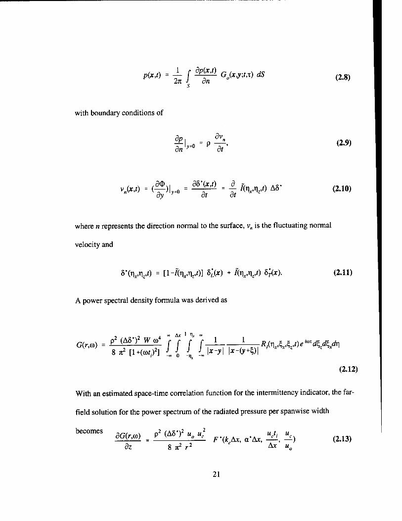
P(x,t) - ± f ^ä Go(r j;r,t) dS 2JI J on (2.8)
with boundary conditions of
dp. dt
(2.9)
, . /SO., d5"(x,t) d ?, ,x A2» (2.10)
where n represents the direction normal to the surface, v„ is the fluctuating normal
velocity and
8*(ti ,v) = [1-%V)] 5t^) + %'V) 6^)- (2.11)
A power spectral density formula was derived as
Ax '"I* «
G(r,co) = p2 (AS*)2 W co4
STtMl+K)2] _ 0 _n +(cof.)2i J J„ J J jf-^l l*-(y+§)l
(2.12)
With an estimated space-time correlation function for the intermittency indicator, the far-
field solution for the power spectrum of the radiated pressure per spanwise width
öz 8 Tt2 r2 c Ax «0
(2.13)
21
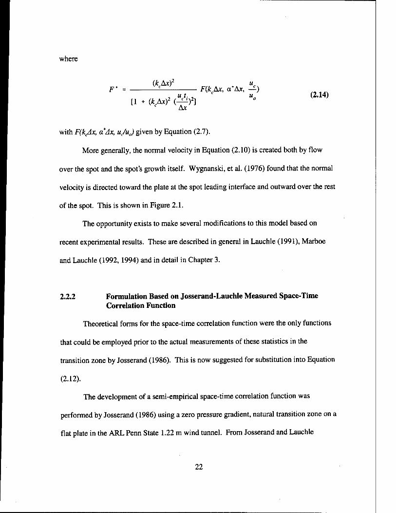
where
F* (k&x)2
[1 + (kcAx)2 (-^i)2] Ax
F(k Ax, a*Ax, —) (2.14)
with F(k<Ax, a Ax, u/u0) given by Equation (2.7).
More generally, the normal velocity in Equation (2.10) is created both by flow
over the spot and the spot's growth itself. Wygnanski, et al. (1976) found that the normal
velocity is directed toward the plate at the spot leading interface and outward over the rest
of the spot. This is shown in Figure 2.1.
The opportunity exists to make several modifications to this model based on
recent experimental results. These are described in general in Lauchle (1991), Marboe
and Lauchle (1992,1994) and in detail in Chapter 3.
2.2.2 Formulation Based on Josserand-Lauchle Measured Space-Time Correlation Function
Theoretical forms for the space-time correlation function were the only functions
that could be employed prior to the actual measurements of these statistics in the
transition zone by Josserand (1986). This is now suggested for substitution into Equation
(2.12).
The development of a semi-empirical space-time correlation function was
performed by Josserand (1986) using a zero pressure gradient, natural transition zone on a
flat plate in the ARL Penn State 1.22 m wind tunnel. From Josserand and Lauchle
22
(1990):
WW,t) = y. Y- * Yu (IT-) «P{- 5 (4 + 200 |x-i|) |T-i| } • exJ ^-^ A.I
exp 1260 |T-
15.75A* 1 + 71 |A 1 + 14.2 |A.
(2.15)
exp A |A.
0.0014 + |AJ , + I300|T_t|2
where A = -ln[l-exp(-4.27/Ax)], (units of J* are in meters),
A,. = $ I Ax ,
yu = yC^j and yd = y(rjx+£J when the reference location is upstream of the second
location,
yu - y(rjx+£x) and yd = y(r\x) when the reference location is downstream of the
second location.
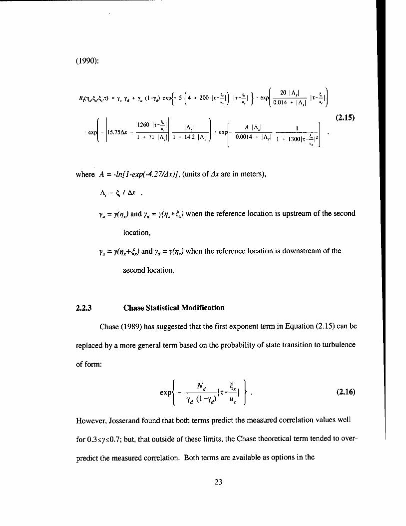
2.2.3 Chase Statistical Modification
Chase (1989) has suggested that the first exponent term in Equation (2.15) can be
replaced by a more general term based on the probability of state transition to turbulence
of form:
exp A7, i
YrfU-Yrf) uc (2.16)
However, Josserand found that both terms predict the measured correlation values well
for 03zyz0J; but, that outside of these limits, the Chase theoretical term tended to over-
predict the measured correlation. Both terms are available as options in the
23
computational codes developed for this dissertation.
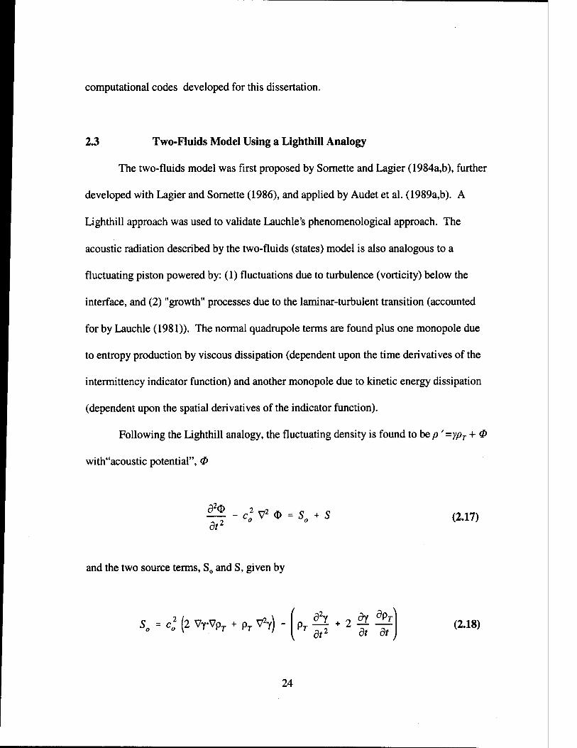
2.3 Two-Fluids Model Using a Lighthill Analogy
The two-fluids model was first proposed by Sornette and Lagier (1984a,b), further
developed with Lagier and Sornette (1986), and applied by Audet et al. (1989a,b). A
Lighthill approach was used to validate Lauchle's phenomenological approach. The
acoustic radiation described by the two-fluids (states) model is also analogous to a
fluctuating piston powered by: (1) fluctuations due to turbulence (vorticity) below the
interface, and (2) "growth" processes due to the laminar-turbulent transition (accounted
for by Lauchle (1981)). The normal quadrupole terms are found plus one monopole due
to entropy production by viscous dissipation (dependent upon the time derivatives of the
intermittency indicator function) and another monopole due to kinetic energy dissipation
(dependent upon the spatial derivatives of the indicator function).
Following the Lighthill analogy, the fluctuating density is found to bep '=ypT + <£
with"acoustic potential", 0
32<J> 2 „2
dv -c0W=S0 + S (2.17)
and the two source terms, S0 and S, given by
S0 = c] (2 VrVpr + pr V2y) d2J x 0 dy dPr VT dt2 dt dt
(2.18)
24
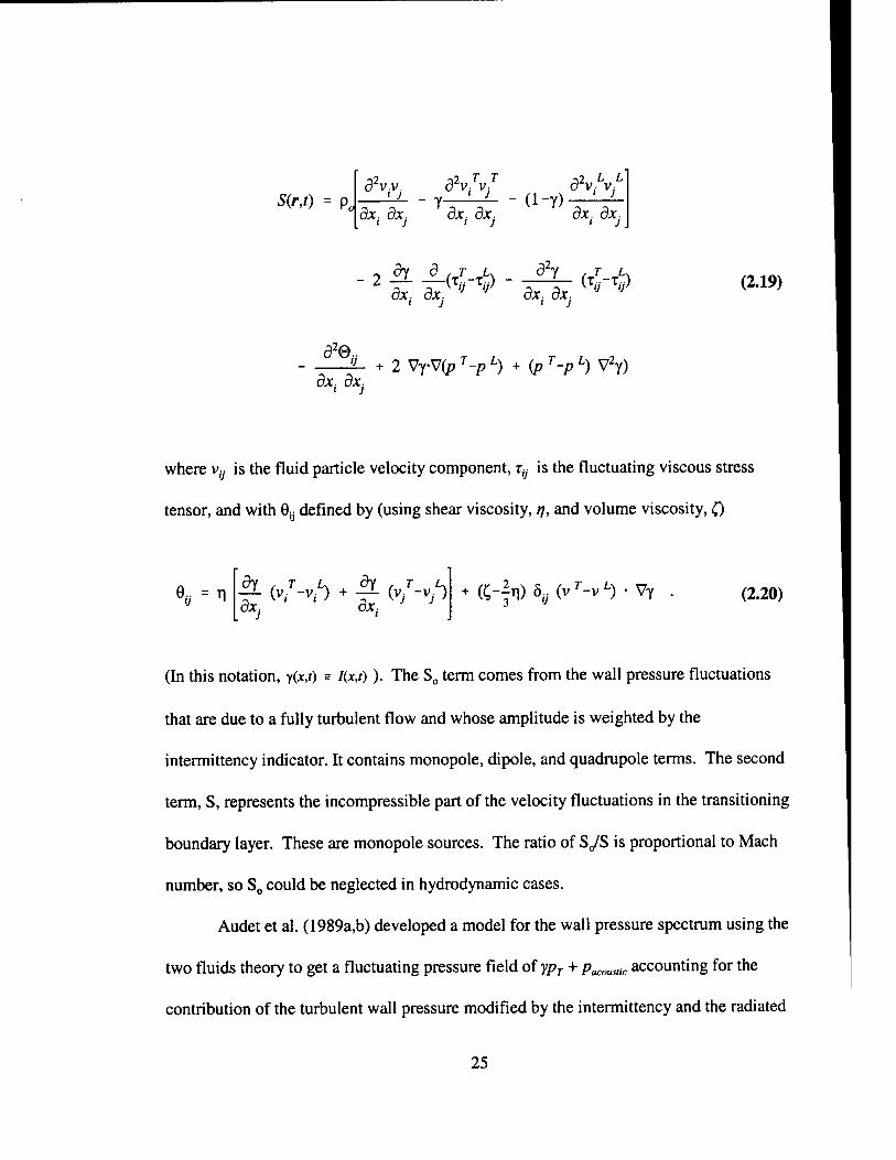
S(r,t) = po
d2w. ' J
dxt dXj dx. dx.
-a T T -a L L d v, v, d v, v, ' J ~ (1-Y) '
dx. dx.
dx( 8xj,J l]) dxt dXj K ,J ,j) (2.19)
a2© dxt dx-
'J- + 2 VyV(p T-p L) + (p T-p L) V2y)
where v,y is the fluid particle velocity component, r0 is the fluctuating viscous stress
tensor, and with Gy defined by (using shear viscosity, rj, and volume viscosity, 0
««=1 dy , r L, dy , T i~ + (C-fn)5,y(v7'-vL)-Vy (2.20)
(In this notation, y(x,0 s /(x,/)). The S0 term comes from the wall pressure fluctuations
that are due to a fully turbulent flow and whose amplitude is weighted by the
intermittency indicator. It contains monopole, dipole, and quadrupole terms. The second
term, S, represents the incompressible part of the velocity fluctuations in the transitioning
boundary layer. These are monopole sources. The ratio of SJS is proportional to Mach
number, so S0 could be neglected in hydrodynamic cases.
Audet et al. (1989a,b) developed a model for the wall pressure spectrum using the
two fluids theory to get a fluctuating pressure field of ypT + p^^c accounting for the
contribution of the turbulent wall pressure modified by the intermittency and the radiated
25
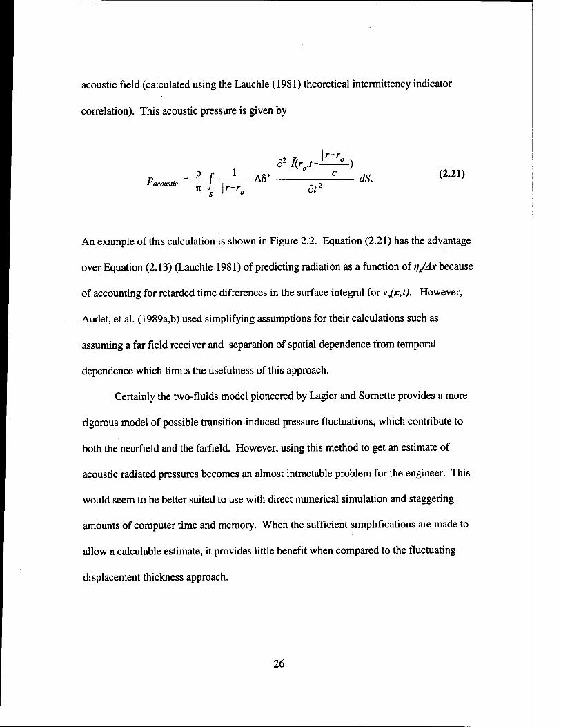
acoustic field (calculated using the Lauchle (1981) theoretical intermittency indicator
correlation). This acoustic pressure is given by
acoustic P r L it ' Ir-r
d2 Kro,t-±-^) A5* - dS.
dt2 (2.21)
An example of this calculation is shown in Figure 2.2. Equation (2.21) has the advantage
over Equation (2.13) (Lauchle 1981) of predicting radiation as a function of rj/Ax because
of accounting for retarded time differences in the surface integral for vn(x,t). However,
Audet, et al. (1989a,b) used simplifying assumptions for their calculations such as
assuming a far field receiver and separation of spatial dependence from temporal
dependence which limits the usefulness of this approach.
Certainly the two-fluids model pioneered by Lagier and Sornette provides a more
rigorous model of possible transition-induced pressure fluctuations, which contribute to
both the nearfield and the farfield. However, using this method to get an estimate of
acoustic radiated pressures becomes an almost intractable problem for the engineer. This
would seem to be better suited to use with direct numerical simulation and staggering
amounts of computer time and memory. When the sufficient simplifications are made to
allow a calculable estimate, it provides little benefit when compared to the fluctuating
displacement thickness approach.
26
2.4 Vortex Motions
Kambe and Minota (1981) and later Kambe (1984, 1986) used the viscosity terms
for vortices to predict quadrupole and low amplitude monopole-like radiation from vortex
motion particularly vortex-edge interaction. According to Kambe (1986), the transition
process evolves from Tollmien-Schlichting waves which are amplified and become
associated with the concentration of vorticity along discrete lines. These lines distort into
vortex loops which continue to distort and grow as turbulent spots until coalescence. The
stresses at the vortex interface become a significant sound source.
Hardin (1991) argues that, by a process of elimination, the major source of sound
in the turbulent boundary layer is the formation of horseshoe vortex structures by the
interaction of the streamwise vorticity with the primary spanwise vorticity. This may be
an important source of sound, in addition to the normal velocity of the fluctuating
displacement thickness.
There have been many advocates of vortex noise generation modeling. The
leaders have been Powell (1964,1995), Obermeier (1977,1979, 1980,1985), Mohring
(1978), Howe (1998a,b, 1999a,b), and Mohring et al. (1983). The dynamic response of a
vortex to interaction with a sound field [Lund, 1989], a surface [Kambe, Minota, and
Dcushima, 1985], and another vortex [Kambe and Minota, 1983] have all been measured
experimentally. Two additional experiments have yielded good qualitative data for
vortex formation behind a vortex generator [Littell and Eaton, 1991] and in boundary
layer transition [Williams, Fasel, and Hama, 1984].
While some aspects of vortex motions are incorporated in the fluctuating
27

displacement thickness and two-fluids models, they probably have not been fully
accounted for in the computational approximations for the normal velocity and therefore
warrant being highlighted as an additional modeling possibility.
The contribution of vortex sound could also play more of a role in flows with non-
zero pressure gradients due to growth and stretching.
2.5 Direct Numerical Simulation
The state of the art in computational fluid dynamics application to solution of the
acoustic problem in fluid flow can be best summarized with a quote from Crighton
(1975):
"Lack of knowledge of features of the flow does not entitle us to make
assumptions and approximations except with the greatest care. We are
dealing with a small by-product, and approximations which may be quite
safe as far as the flow dynamics are concerned may be fatal for the by-
product. Vast errors may easily be incurred in this way through
apparently harmless approximations, especially in underwater flows,
where the Mach numbers are always extremely small, and the acoustic
energy is a correspondingly minute fraction of the total energy.... Highly
accurate numerical predictions are simply not to be expected - a reflection
of the fact that noise levels usually vary far more widely than do the
parameters which describe the noise-producing flow."
Having read that, it is important to state that significant progress has been made in
28

the last eight years. Some of the best work has been done by Wang, Lele, and Moin
(1994,1996a, 1996b). Their modeling focuses on the quadrupole source functions in the
solution of the full incompressible Navier-Stokes equations. They find that negligible
sound is created during primary and secondary instability stages but that disintegration of
the detached high shear layer and vortex shedding near the boundary layer edge results in
amplification of the Reynolds stress quadrupoles, particularly at the frequency of vortex
shedding. Their conclusion is that the acoustic quadrupoles and images dominate up
through the formation of spots and then in-plane dipoles, due to surface shear stress,
dominate in late transition. [Note that this is the modeling approach of Lauchle (1980)
discussed in section 2.1]. The small scale features and large convected eddies are
considered to be inefficient acoustic sources despite larger amounts of energy. They also
show that small structures traveled faster than the lambda vortex which elongates the
disturbance region yet neighboring spot interaction is negligible. This group has also
developed a hybrid technique for low Mach numbers that uses a Navier-Stokes solver for
incompressible hydrodynamic terms and a Lighthill analogy for the acoustic contribution.
Notably, an exit boundary correction is also been developed for the quadrupole source
calculated in the truncated domain, V0
Qif» - Jl / W) d'y + fj Uc Tfi*) d2y (2.22)
given by the second term which is equal to the time derivative of the Lighthill stress
fluxes carried by convecting eddies across the exit surface. In contrast, Kloker,
29
Konzelmann, and Fasel (1993) use a "re-laminarization" zone downstream of transition
before passing through the outflow boundary to suppress reflected flow disturbances in
direct numerical simulation (DNS).
A very important part of any DNS modeling effort is the introduction of a
disturbance to cause breakdown to turbulence. An excellent overview is provided in Rist
and Fasel (1995). They discuss the use of temporal vs. spatial models. They recommend
that most "real life" cases should only use a spatial model, but the penalty is in processing
resources. They also discuss a mean flow which is obtained from a time averaged
disturbance flow. This quantity is like what Krane (1992) measured. This is contrasted
with a steady base flow that is obtained from numerical solution of the Navier-Stokes
equations before the unsteady flow field is calculated. They also found a high shear layer
structure that sat on top of the lambda vortex structure and instantaneous maps of normal
velocity (see Figure 2.3) that show a pushing of the flow structures away from the wall.
A number of computational studies have achieved results which may contribute to
our qualitative understanding of transitional flow structures. Coherent structures, similar
to bursts in the fully developed TBL, were calculated by Rempfer and Fasel (1994).
There is a spike stage in their result which yields fluctuating velocities that are significant
for acoustic modeling. Ducros et al. (1996) performed a large eddy simulation (LES) of
boundary layer transition. This took 80 hours (CRAY YMP) using LES (compared to
800 hours using DNS, Rai and Moin (1993)) and a filtered structure function on the
velocity field to eliminate large scale oblique perturbations. Their results show
qualitative progress and could aid in interpretation of the role of vorticity in the acoustic
30
signature. But obviously, this is not a time effective means for prediction or design.
Yang, et al. (1992) performed computational analyses for natural transition in an adverse
pressure gradient. Similarly, the works of Goldstein et al. (1992), Goldstein and Leib
(1993), plus Henningson and Kim (1991) show results which provide some insight into
the roles of vorticity, local separations, and spot growth. Wilde and Rose (1997)
concluded from their use of a temporal model of K-type transition and spatial model of
bypass transition that the generated sound comes from the streamwise dipole of the wall
shear stress.
The work of Joslin (1991) on the modeling of the effects of compliant walls on
primary and secondary instabilities in boundary layer transition warrants further
investigation relative to efficient numerical simulation compared to DNS. This may also
have some applicability in further refining the fluctuating displacement thickness model.
Abraham and Keith (1997) have shown that DNS simulations for the fully
developed TBL can produce a reasonable estimate for wall pressure events associated
with sweeps and bursts. They also show that the number of positive and negative events
occur in comparable densities and that their average spectra are lower in level by 3 to 7
dB than their peak spectral amplitudes. This is significant in light of the positive and
negative normal velocity distributions sensed for the passage of for turbulent spots
described in Krane and Pauley (1995).
31

2.6 Direct and Indirect Radiation From Complex Geometries
The research described here is intended to critically examine the popular
approaches to modeling the radiation mechanisms and bring some degree of closure to the
physical and practical significance of noise and pseudo-noise originating in the laminar-
to- turbulent transition zone within a natural boundary layer. This effort includes
updating of models to include recent computational and experimental statistics plus an
evaluation of model sensitivities, applicability, and significance for situations of
engineering relevance such as for the noses of bodies of revolution and for airfoils.
Although little has yet been done to model transition noise for transition zones
specifically on curved surfaces, Howe (1981) has made some generalizations. He
contends that displacement thickness fluctuations will give efficient sound radiation in
the regions of a surface or body where the local radius of curvature is smaller than the
acoustic wavelength. For an airfoil, this would be in the leading and trailing edge regions
under compact conditions.
2.6.1 Vicinity of a Half-Plane Leading Edge
The effect of scattering of near-field energy due to the surface geometry near the
leading edge or trailing edge of a plane is to enhance the shear stress dipole sources in the
transition region based on formulations by Howe (1999a,c). These sources may be less
important for flat walls compared to the quadrupole sources in the turbulent spots but, for
a curved leading edge, tend to contribute to the low frequency signature following a U6
velocity scaling. Two factors play into this. First, due to the curvature of the leading
32
edge, the transition tends to occur in a region of adverse pressure gradient which will
accelerate the transition. Second, the nearfield of the transition region hydrodynamic
unsteadiness will extend forward to the leading edge and diffract around the curved
surface.
Howe models the transition region with an 'upwash' velocity on the body surface
using the Biot-Savart formula giving the (time dependent) distributed vorticity induced
instantaneous velocity field as though the surface was not present. He uses the
proportional local blocked surface pressure to represent the spectrum of the upwash
velocity. The fully developed TBL spectrum is used with the addition of an intermittency
weighting factor.
The assumptions for this model include:
very low Mach number, 2-D flow;
symmetric, finite thickness plane (better termed a hydrofoil);
hydrofoil chord is acoustically non-compact;
hydrofoil span is much greater than the boundary layer thickness;
hydrofoil thickness is acoustically compact, and that the leading edge is within the
nearfield of the transition zone;
zero angle of attack and boundary layer fluctuations on opposite sides of the foil
are equal and independent so an estimate of one side can just be increased by 3
dB;
the integration of the vorticity is restricted to the non-linear region of the
boundary layer above the viscous sublayer, so bound vorticity on the hydrofoil is
33
ignored; and
• high Reynolds number, the contribution of tangential shear stresses is ignored.
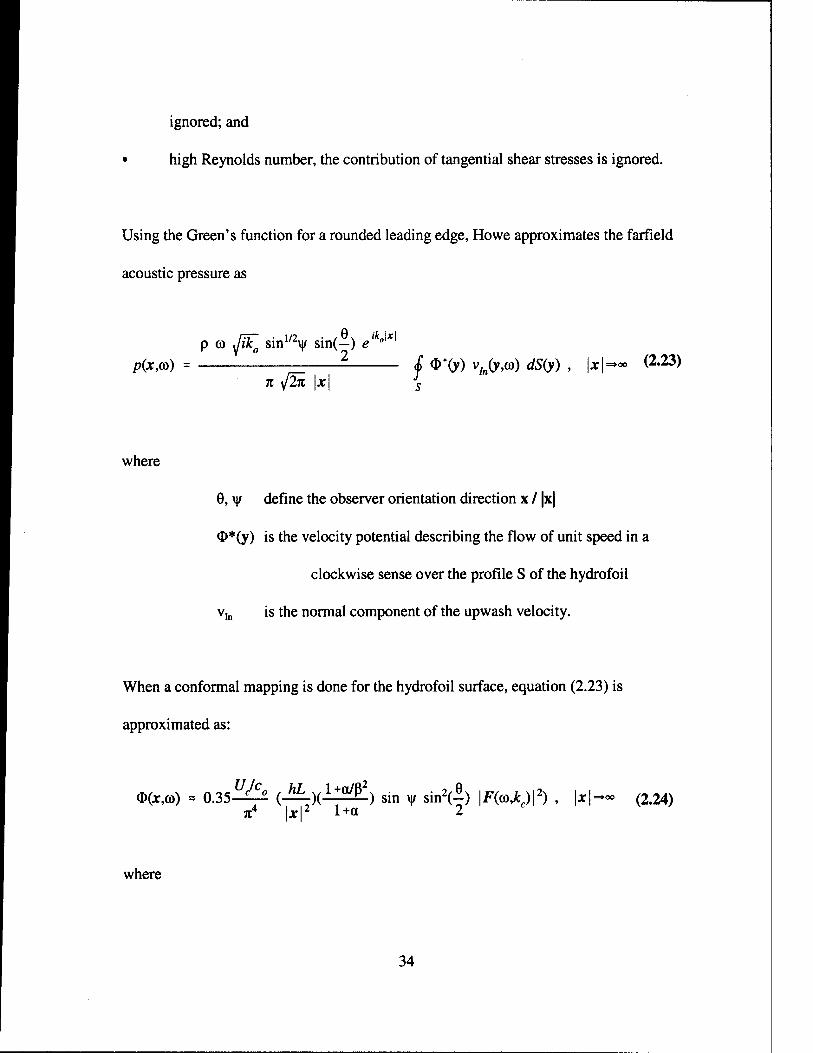
Using the Green's function for a rounded leading edge, Howe approximates the farfield
acoustic pressure as
,1/2,,. „:„/9\ Jk0\x\ p (0 Jiko sin1 \|/ sin(—) e p(x,o>) = £ 0*(y) vIn(y,(o) dS(y) , |x|-» (2-23>
K \JlJl \X\ 5
where
0, \|/ define the observer orientation direction x / |x|
<D*(y) is the velocity potential describing the flow of unit speed in a
clockwise sense over the profile S of the hydrofoil
vto is the normal component of the upwash velocity.
When a conformal mapping is done for the hydrofoil surface, equation (2.23) is
approximated as:
<D(X,(ö) * 0.35-^ (_*L)(1^) sin ¥ sin2A \F((o,kc)\2) , |x|-«- (2M)
7t4 Ixl2 l+a
where
34
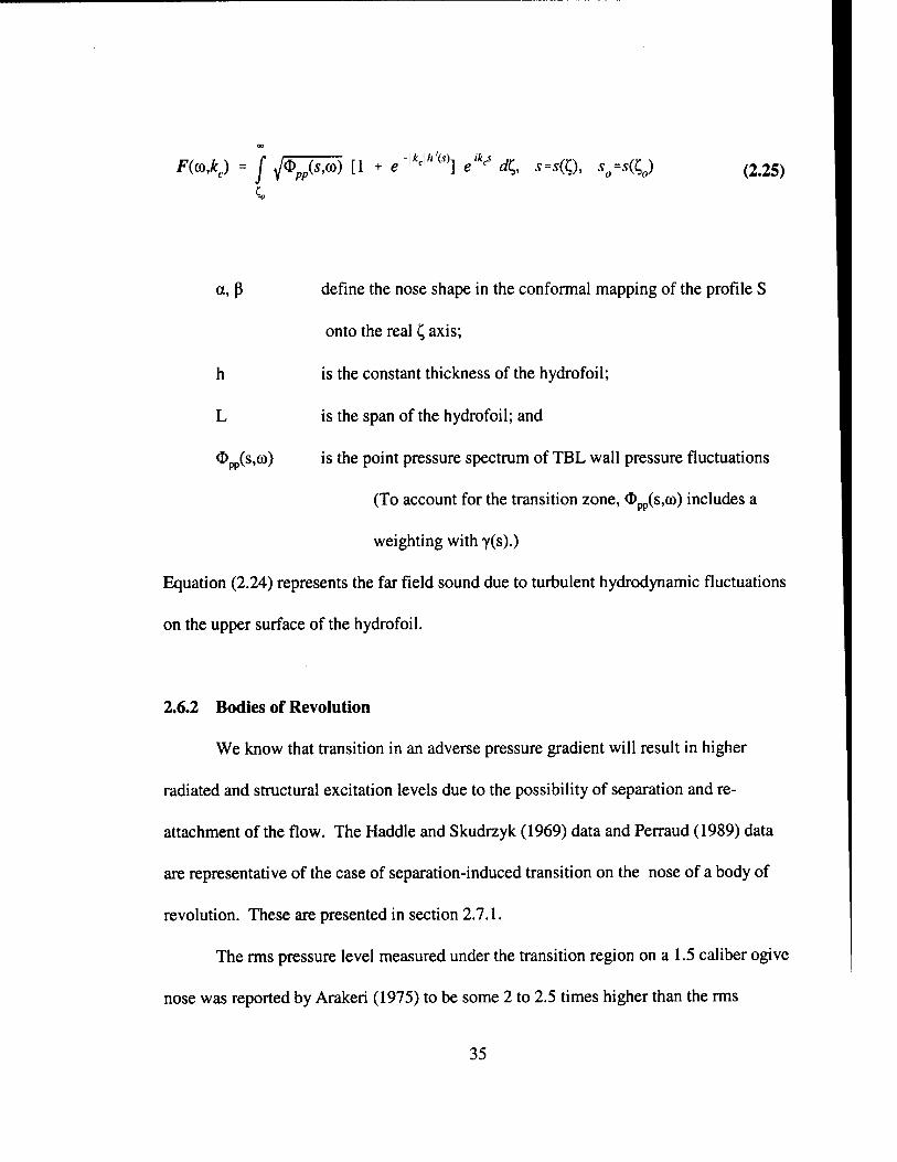
-\kc\h\sU iV F(a>,kc) = f JÖJf&j [1 + e'^"n e'^ %, s=s(Q, so=s(Q (2.25)
a, ß define the nose shape in the conformal mapping of the profile S
onto the real £ axis;
is the constant thickness of the hydrofoil;
is the span of the hydrofoil; and
is the point pressure spectrum of TBL wall pressure fluctuations
(To account for the transition zone, Opp(s,co) includes a
weighting with y(s).)
Equation (2.24) represents the far field sound due to turbulent hydrodynamic fluctuations
on the upper surface of the hydrofoil.
h
L
#PP(S,CO)
2.6.2 Bodies of Revolution
We know that transition in an adverse pressure gradient will result in higher
radiated and structural excitation levels due to the possibility of separation and re-
attachment of the flow. The Haddle and Skudrzyk (1969) data and Perraud (1989) data
are representative of the case of separation-induced transition on the nose of a body of
revolution. These are presented in section 2.7.1.
The rms pressure level measured under the transition region on a 1.5 caliber ogive
nose was reported by Arakeri (1975) to be some 2 to 2.5 times higher than the rms
35
pressure measured further back under the fully developed TBL. The hemispherical nose
shape does promote laminar separation and the rms pressure levels measured in and
around the separation reattachment point are 10 times higher than the TBL rms pressure
levels. The separation-induced wall pressure fluctuations are 4 to 5 times higher than
those induced by transition. Similar measurements were performed by Huang and Shen
(1989). Several axisymmetric headforms were tested in the Anechoic Flow Facility at
David Taylor Model Basin where wall pressure fluctuations induced by either natural
transition or laminar separation were determined. They arrived at the same conclusions
as Arakeri regarding the magnitude of the pressure fluctuations.
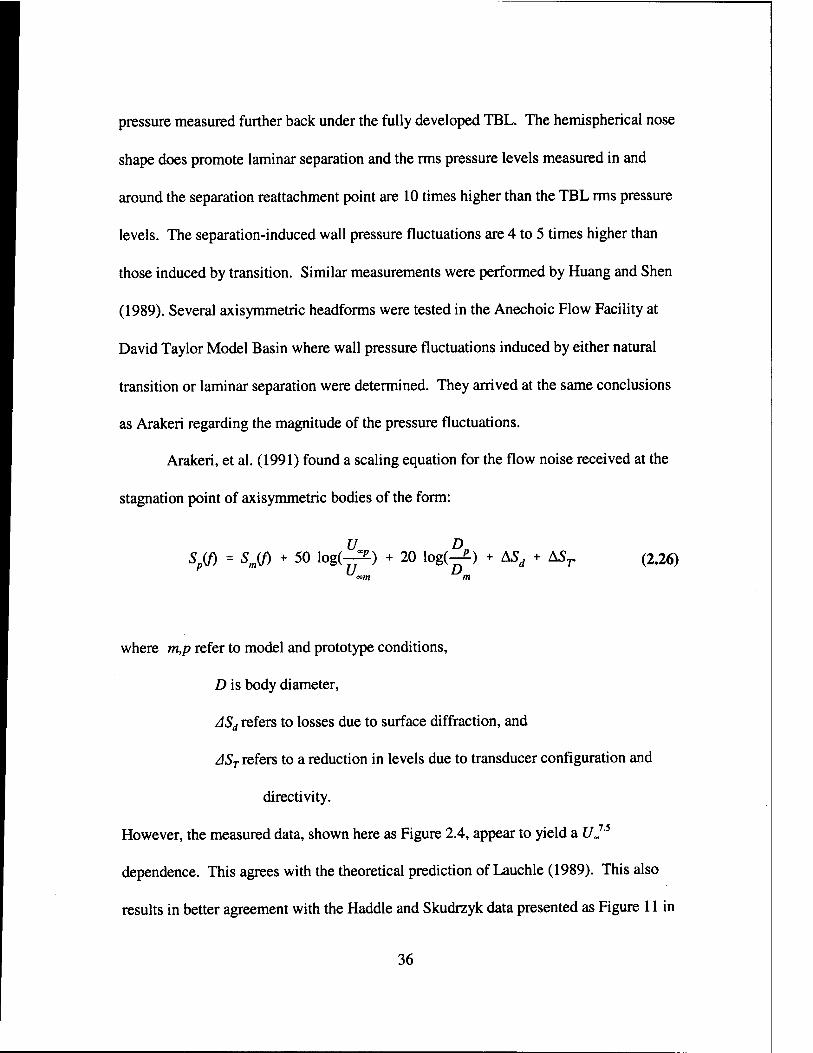
Arakeri, et al. (1991) found a scaling equation for the flow noise received at the
stagnation point of axisymmetric bodies of the form:
Sp<f> = sm<f) + 50 log(~*) + 20 log(-£) + ASd * ASr (2.26)
where m,p refer to model and prototype conditions,
D is body diameter,
ASd refers to losses due to surface diffraction, and
AST refers to a reduction in levels due to transducer configuration and
directivity.
However, the measured data, shown here as Figure 2.4, appear to yield a Uj5
dependence. This agrees with the theoretical prediction of Lauchle (1989). This also
results in better agreement with the Haddle and Skudrzyk data presented as Figure 11 in
36
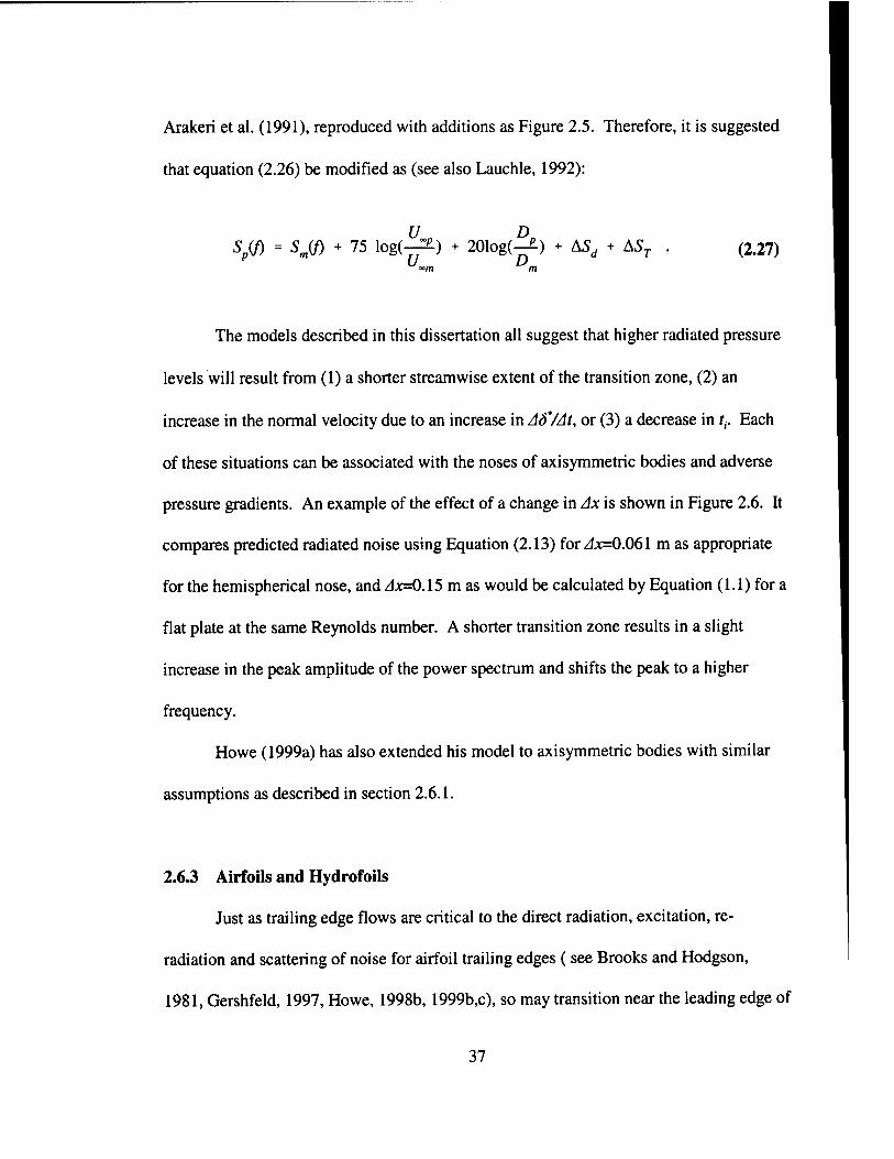
Arakeri et al. (1991), reproduced with additions as Figure 2.5. Therefore, it is suggested
that equation (2.26) be modified as (see also Lauchle, 1992):
Sp(/) = SJf) + 75 log(-^) + 201ogA) + ASd + AST . (2.27)
The models described in this dissertation all suggest that higher radiated pressure
levels will result from (1) a shorter streamwise extent of the transition zone, (2) an
increase in the normal velocity due to an increase in AS'/At, or (3) a decrease in tt. Each
of these situations can be associated with the noses of axisymmetric bodies and adverse
pressure gradients. An example of the effect of a change in Ax is shown in Figure 2.6. It
compares predicted radiated noise using Equation (2.13) for J.x=0.061 m as appropriate
for the hemispherical nose, and Ax=QA5 m as would be calculated by Equation (1.1) for a
flat plate at the same Reynolds number. A shorter transition zone results in a slight
increase in the peak amplitude of the power spectrum and shifts the peak to a higher
frequency.
Howe (1999a) has also extended his model to axisymmetric bodies with similar
assumptions as described in section 2.6.1.
2.6.3 Airfoils and Hydrofoils
Just as trailing edge flows are critical to the direct radiation, excitation, re-
radiation and scattering of noise for airfoil trailing edges ( see Brooks and Hodgson,
1981, Gershfeld, 1997, Howe, 1998b, 1999b,c), so may transition near the leading edge of
37
an airfoil act as a noise source. Of course, the characteristics of the transition location
and extent is quite dependent upon the chordwise distribution of thickness for the airfoil.
This is well discussed in the papers by Halstead et al. (1995a,b,c,d) and Lou and
Hourmouziadis (1999). These investigations encompassed operation with periodic flows
due to upstream blade wakes in the former and a downstream rotating flapper valve in the
latter reference. Transition as well as laminar separation and turbulent reattachment were
observed. However, in that case, the growth of the instability did not match that for
natural transition on a flat plate. It was suggested by Wilde and Rose (1997) that
transition noise may be most important in cases where the surface area covered by
transitioning flow is comparable to fully turbulent flow area. This is potentially the case
with airfoils used in turbines which encounter bypass and separation-induced transition
due to inflow wakes (Addison and Hodson, 1991 and Halstead et al., 1995a,b,c,d). The
applicability of any of the reviewed models for transitional flow on blades would most
likely be the substitution of the appropriate leading edge Green's function into the
fluctuating displacement thickness model following the work of Howe (1998,1999a).
2.7 Need for Refining the Fluctuating Boundary Layer Displacement Thickness Model in a Natural Transition Region
It is now possible to make some refinements to the Lauchle (1981) model with the
availability of the empirically derived Josserand space-time correlation function
(Josserand and Lauchle, 1990). It should be noted that a similar treatment can also be
incorporated into the two-fluids model.
38
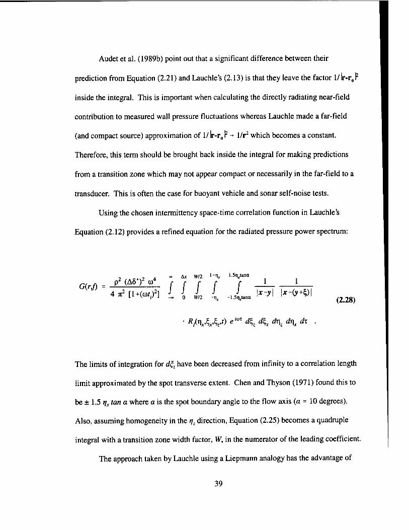
Audet et al. (1989b) point out that a significant difference between their
prediction from Equation (2.21) and Lauchle's (2.13) is that they leave the factor 1/ lr-r012
inside the integral. This is important when calculating the directly radiating near-field
contribution to measured wall pressure fluctuations whereas Lauchle made a far-field
(and compact source) approximation of 1/ lr-r012 - 1/r2 which becomes a constant.
Therefore, this term should be brought back inside the integral for making predictions
from a transition zone which may not appear compact or necessarily in the far-field to a
transducer. This is often the case for buoyant vehicle and sonar self-noise tests.
Using the chosen intermittency space-time correlation function in Lauchle's
Equation (2.12) provides a refined equation for the radiated pressure power spectrum:
1 ■> ..c.,9 ± °° Ax W/2 l~\ l-5Vana
__ P'(AS")' o, . . , , ,1 _^ 4 Tt2 ri+rtüM2l J J J J J jc-v Jt-(y+c) t 71 UTVWyJ _„ o VV/2 -i)x -l^tana ' "" ' v T/' (2.28)
Rfi\A&fi eim d^z ^ d\ d\ dx
The limits of integration for d£z have been decreased from infinity to a correlation length
limit approximated by the spot transverse extent. Chen and Thyson (1971) found this to
be ± 1.5 tjx tan a where a is the spot boundary angle to the flow axis (a ~ 10 degrees).
Also, assuming homogeneity in the rjz direction, Equation (2.25) becomes a quadruple
integral with a transition zone width factor, W, in the numerator of the leading coefficient.
The approach taken by Lauchle using a Liepmann analogy has the advantage of
39
being able to incorporate both the gross piston like fluctuation of the boundary layer
displacement thickness and the acoustic sources associated with the growth of the spot
domain involving the horseshoe vortex. The gross piston fluctuation is described by Ab",
Ax, uc, tj and N. The spot size limitation is accounted for by 1.5 tjx tan a. Whatever spot
dynamics (and resulting unsteady pressure sources) haven't been accounted for properly
in an empirically derived space-time correlation at the wall will become the necessary
future refinements.
In trying to identify these, some useful information has been found on spot
statistics in Wygnanski et al. (1976). Experimental evidence was cited to establish that
two artificially generated spots displaced laterally did not affect each others' growth rate.
They also provide detailed descriptions of spot dynamics as shown in Figures 2.7 and 2.8.
The spot shape as a function of normalized surface point passage time in Figure 2.7
shows the variation of the extent of the spot with height off the surface. This variation is
important when trying to model the spatial distribution of normal velocity to define the
motion of an equivalent "piston". The variation of v„ with normalized time at two
elevations (Figure 2.8) shows how difficult it is to define vjn^n^t). The celerity of the
spot's leading and trailing edges vary with v. Gutmark and Blackwelder (1987) reported
measuring leading and trailing edge celerities which increased with y from 0.881L and
0.5SU„ at y^O.lb^ to Q.9W„ and 0.60£/„ at y=Slam. Similar results were found from data
of other investigators.
40
2.7.1 Example Applications of Fluctuating Displacement Thickness Model
Measurements of wall pressures and an apparent upstream acoustic propagation of
transition zone emissions have been made on an axisymmetric 0.32 m diameter body in
the CEPRA 19 anechoic wind tunnel by Perraud (1989). Comparisons are made to
pressure spectra measured using large flush-mounted transducers. In this experiment,
r = 0.3 m, Ax = 0.20 m, u/U„ = 0.8, and AS* was estimated to be 0.25 mm. The spectral
shape and amplitude were predicted reasonably well with 0.05 <, uj/Ax <, 0.15.
Computational results are compared to the measured data in Figure 2.9. Low-
frequency energy appears centered around the most unstable Tollmein-Schlichting wave
frequencies; this contribution is not predicted by the current theoretical model.
A comparison is also made of predicted radiated noise to the buoyant body data of
Haddle and Skudrzyk (1969). While there are also contributions from the fully developed
TBL and noise from the stabilizing fins, which were found (Lauchle and Brungart 1988),
using TBL noise estimates from Blake (1986) and Lauchle (1977), and fin trailing edge
noise estimates from Brooks and Hodgson (1981), to be much lower than the measured
noise. Results for a typical operational condition of £/„ = 15.44 m/s, Ax = 0.061 m, r =
1.0 m, uflJ„ = 0.8, body diameter of 0.48 m and AS* estimated as 0.43 mm have been
made. These are all shown in Figure 2.10. The predicted spectral levels for the directly
radiated noise from the fully-developed TBL seems inconsistently low relative to the
predicted transition noise when compared with the airflow measurements described in
Chapter 6. It is believed that several factors may contribute to this. The low wavenumber
data used to estimate the TBL noise may have been underestimated by the wavevector
41
filtering used in the experiment. The scaling relationship used by Blake assumes a rigid
flat wall and also neglects the effect of proximity of the source to a nose of the body as
examined by Howe (1999a). There could also have been some separation and
reattachment of flow near the noise due to slight variation in angle of attack as the
buoyant body ascended.
Neither application of the model is particularly satisfying. Likewise, each of the
examples presented by Lauchle (1981) seem to have the best fit of predicted versus
measured data for non-dimensional rise time, 0.45 < U<t/Ax,< 1.0. However, this tends
to describe only the shape of the higher frequency portion of the spectrum. Clearly,
improvements to the model are in order.
It is important to point out that in underwater flow situations, the common
presence of inhomogeneities, particularly bubbles, can account for a considerable increase
in radiated noise. For example, Crighton (1975) shows that air bubble concentrations
with a void fraction of less than 1% in turbulent flow can increase the radiated noise
power by up to 50 dB due to excitation by passage of the bubbles through high pressure
gradient flows.
2.7.2 Study Objectives: General Approach Towards Characterizing the Acoustic Emissions from Isolated Transition Flow Structures and a Natural Transition Zone
Given the possibility of high radiating energy from the transition zone,
understanding the boundary layer transition process is perhaps as important from the
point of view as a structural excitation mechanism as it is as a direct radiator. It is beyond
42
the scope of this dissertation to pursue all of the fluid-structure coupling implications and
local excitation of bubbles which must be dealt with to truly predict the transition related
signature in an underwater situation. However, this may be the role in which transition is
most important for problems of practical concern. It certainly does not appear that direct
radiation from such a small area as the transition region (and probably only half of it in
terms of spot growth) is significant when compared to fully developed TBL noise over
the surface area of the rest of the body or plane in zero or variable pressure gradients.
Nevertheless, we are interested in pursuing improvements in both aerodynamic and
hydrodynamic modeling of boundary layer transition noise mechanisms and validation
through quality experiments because it is reasoned that transition flow structures form the
basic building blocks of all subsequent downstream flow behavior and its acoustics.
The problem then is that two basic modeling approaches exist for the direct
radiation from a naturally transitioning boundary layer. While the two-fluids model may
be the more inclusive, it is also the more difficult to apply in practice. The
phenomenological Liepmann approach is the most amenable to incorporation of recent
experimental descriptions of the normal velocity fluctuations. This study has
concentrated on Liepmann model modifications and further qualitative assessments. A
series of experiments have been performed for evaluation of the models.
At this point, the value of direct numerical simulation may be to provide insight
on the necessary modeling of substructure dynamics that influence the spatial definition
of the normal velocity used in the fluctuating displacement thickness model, and hence
contribute, in their own right, to the acoustic pressure, particularly that in the nearfield.
43
This bridges the gap, to some extent, between the two-fluids model using the Lighthill
analogy, and the Liepmann approach used for the fluctuating displacement thickness
model.
44
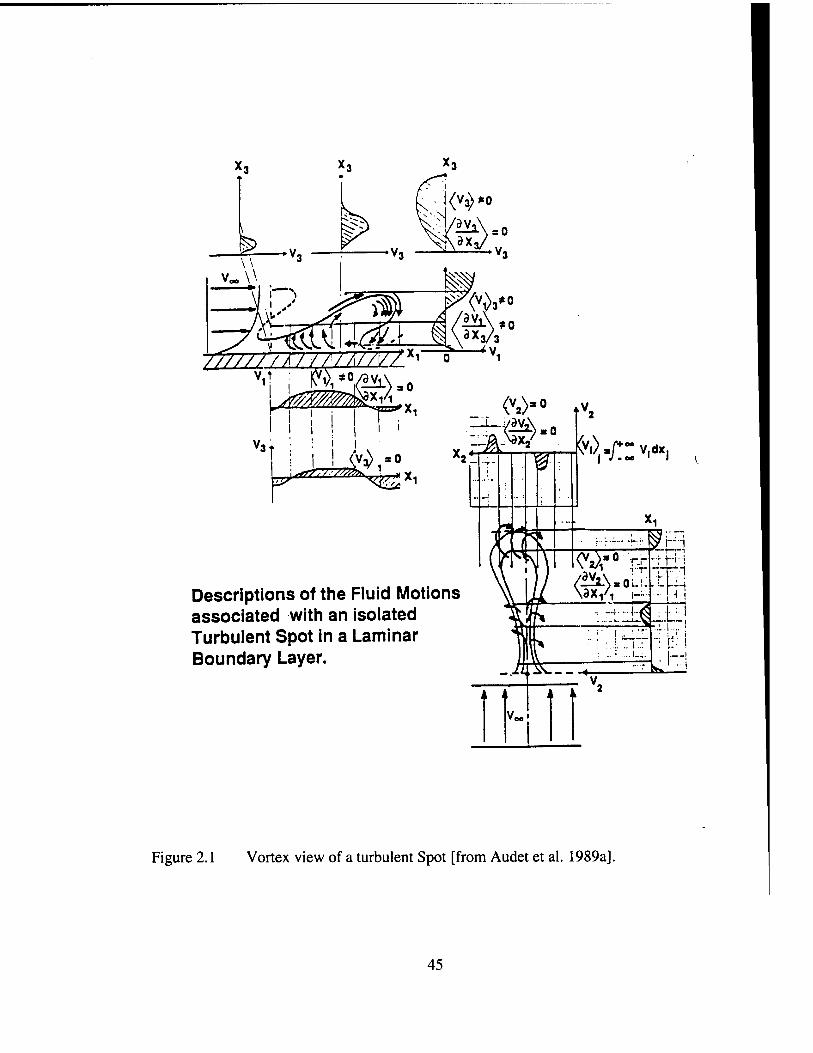
k ■*v.
///////P/7//A//vL^ o vi
'\r^2.
V3t ' '
Descriptions of the Fluid Motions associated with an isolated Turbulent Spot in a Laminar Boundary Layer.
Figure 2.1 Vortex view of a turbulent Spot [from Audet et al. 1989a].
45

1.0 --
p 1/2 pU'
0.5 -
0.25 0.5
x/Ax
0.75
Figure 2.2 The normalized rms wall pressure fluctuations in the transitional boundary layer measured and predicted for a flat plate. The curves are predictions which account for spatial and frequency filtering of the sensors. Curve 1 is ypT, Curve 2 is the radiated acoustic source term, and Curve 3 is their sum. The symbols are measured data for 3 velocities, [from Audet et al. 1989a,b].
46
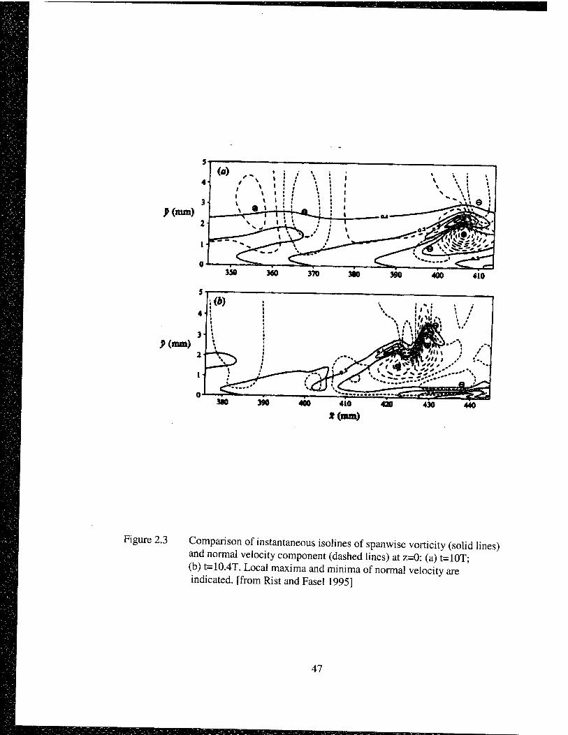
J>(ram)
?(mm)
Figure 2.3 Comparison of instantaneous isolines of spanwise vorticity (solid lines) and normal velocity component (dashed lines) at z=0: (a) t=10T; (b) t=10.4T. Local maxima and minima of normal velocity are indicated, [from Rist and Fasel 1995]
47
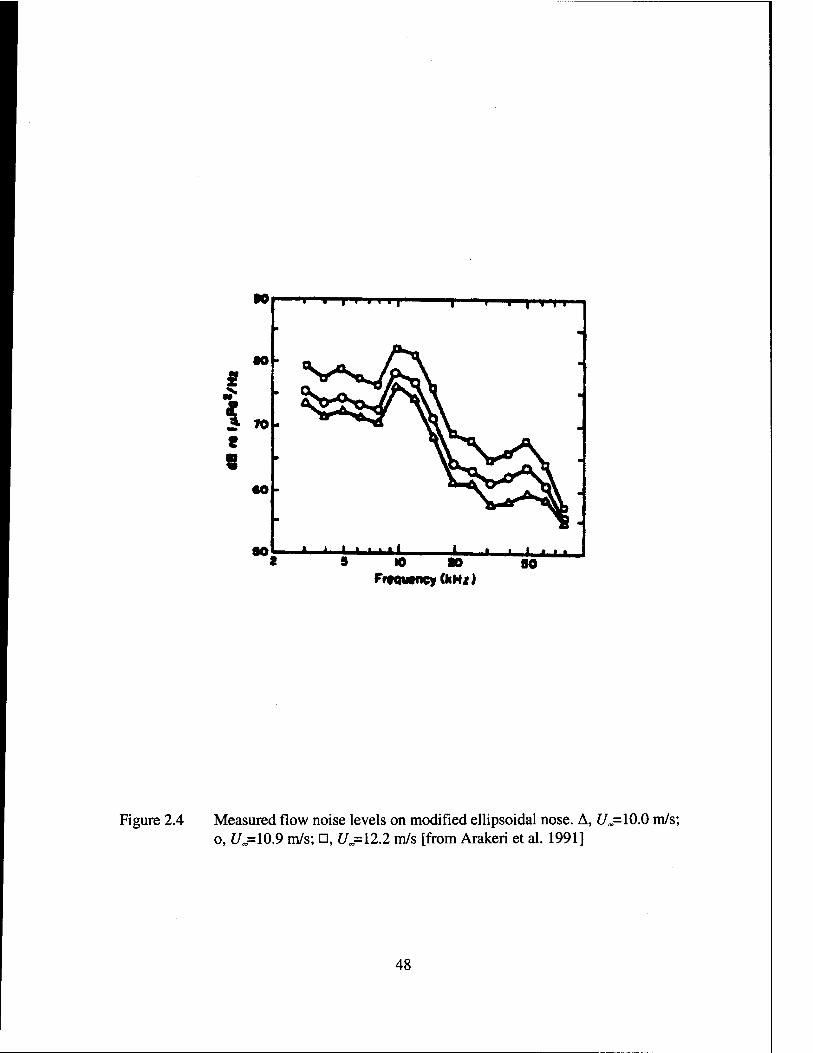
" i" ■ i i i«»r
S
i
to
3 *o t 8
to
so
l't 11
5 10 10 FrtqutncydiHx)
Figure 2.4 Measured flow noise levels on modified ellipsoidal nose. A, £/„=10.0 m/s; o, U=10.9 m/s; □, £/j=12.2 m/s [from Arakeri et al. 1991]
48
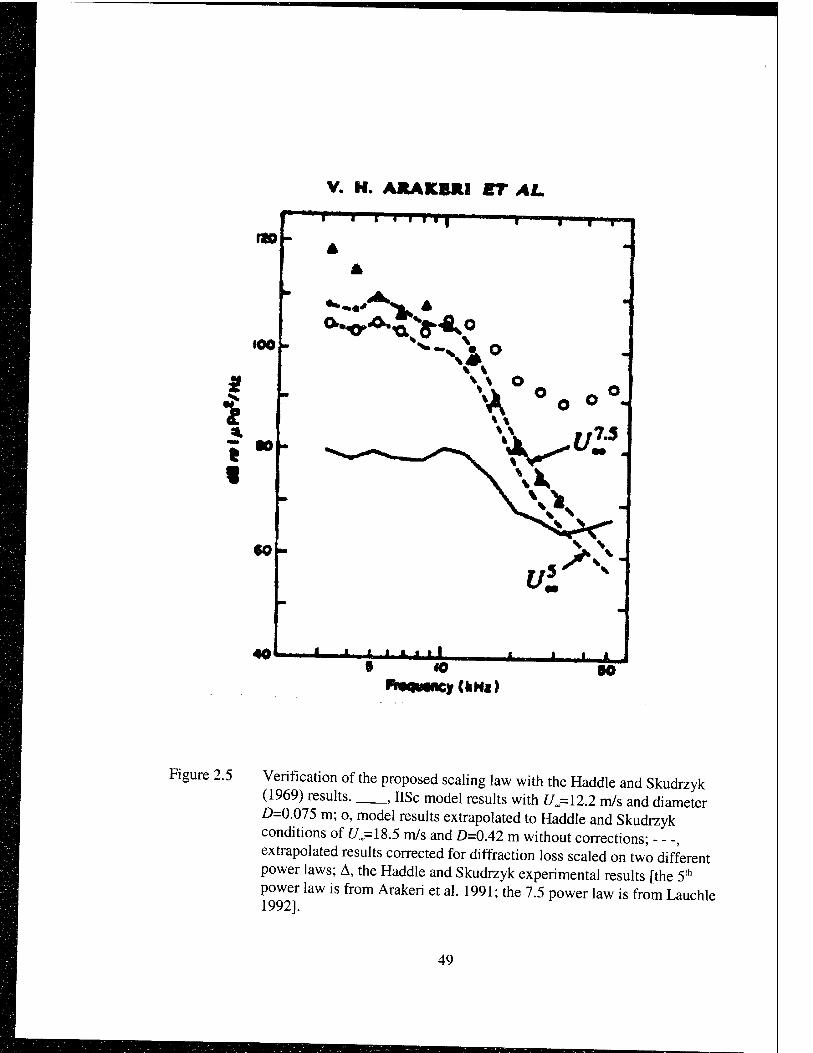
«o
400 -
V. H. ARAKBRI BT AL
r i i i i 111 1 I I r
2
1
60
40 i i r i i i il 10
UN«)
I I I I „i 80
Figure 2.5 Verification of the proposed scaling law with the Haddle and Skudrzyk (1969) results. , HSc model results with U=\2.2 m/s and diameter Z)=0.075 m; o, model results extrapolated to Haddle and Skudrzyk conditions of £/„=18.5 m/s and D=0.42 m without corrections; - - -, extrapolated results corrected for diffraction loss scaled on two different power laws; A, the Haddle and Skudrzyk experimental results [the 5th
power law is from Arakeri et al. 1991; the 7.5 power law is from Lauchle 1992].
49
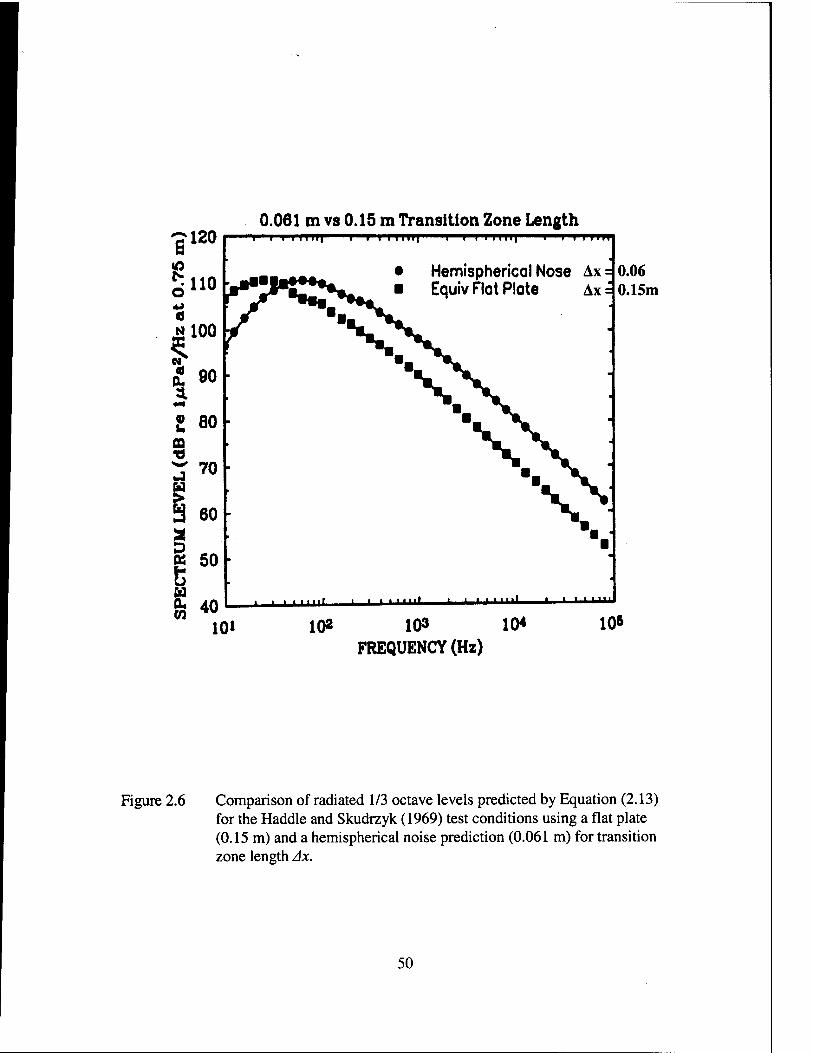
0.061 m vs 0.15 m Transition Zone Length
Hemispherical Nose Ax = Equiv Flat Plate Ax =
101
0.06 0.15m
102 103 10« FREQUENCY (Hz)
10»
Figure 2.6 Comparison of radiated 1/3 octave levels predicted by Equation (2.13) for the Haddle and Skudrzyk (1969) test conditions using a flat plate (0.15 m) and a hemispherical noise prediction (0.061 m) for transition zone length Ax.
50
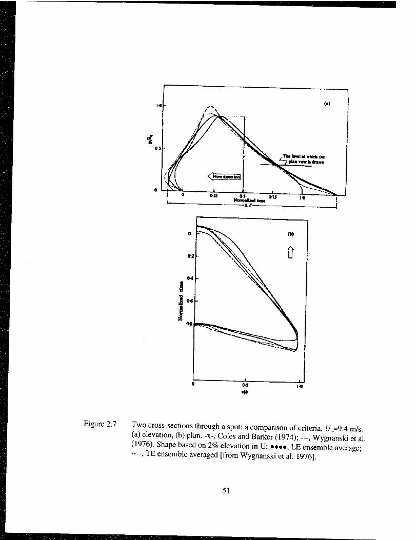
I o o-a
<•)
TKt bvtlM «hick UM pluvswfcdrtwa
0-J 0-7J NaauHndtioM AT
I*
Figure 2.7 Two cross-sections through a spot: a comparison of criteria, U =9.4 m/s (a) elevation, (b) plan, -x-, Coles and Barker (1974); —, Wygnanski et al. (1976). Shape based on 2% elevation in U: ••••, LE ensemble average; —, TE ensemble averaged [from Wygnanski et al. 1976].
51
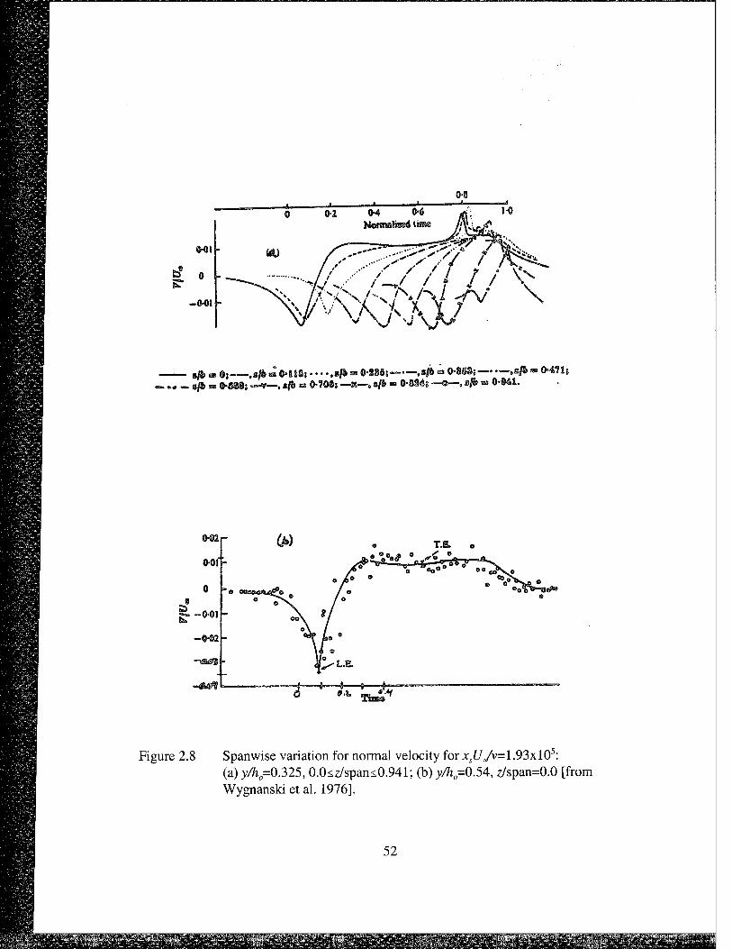
ffi-OI
S" -0-01
f> ■■■■■" / / / / ; / V /^•\ /-. /\./xi <V"\/ x
— s/b ■ ©s ,«/fc ■ <M18s • • • • ,i/6 - 0-288;——,s$ ■ 0-86§s— —1«/& ■ »* — s® » ®-®8S; —■*—. a/& » 0-70®? —X—, s/6 ■>= 0-8M; —©—. »ft> «■ 0-M1.
e-32
0-01"
0
g. -001
-e-02
4 t' »—-i—-4 9.8. n« af Tims
Figure 2.8 Spanwise variation for normal velocity for x5[/yv=1.93xl05: (a) y/h =0.325, 0.0<z/span<0.941; (b) y/h=0.54, z/span=0.0 [from Wygnanski et al. 1976].
52
Bs^aBfijftrasa&S^^
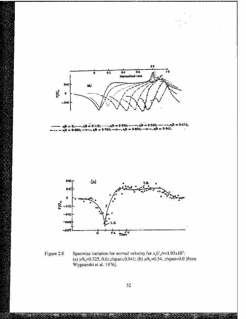
0-2
0-01
-<H>!
0-4 0-6 Ncnwitta^ tits®
10
\<iA jrf*
>/7 / / \:
N.
^^W" v
— s/6 « ©! ,ußm CMI8? • • • -.8/& ■ O-SSfls——.«/k ■» ©-W8; — •—„«/&> - ©"«is
042
CM»"
0
a* S. -001
-©•«2
Figure 2.8 Spanwise variation for normal velocity forxst/yv=1.93xl05: (a) y/h =0.325, 0.0 <z/span< 0.941; (b) y/h=0.54, z/span=0.0 [from Wygnanski et al. 1976].
52
Ijifeff^^
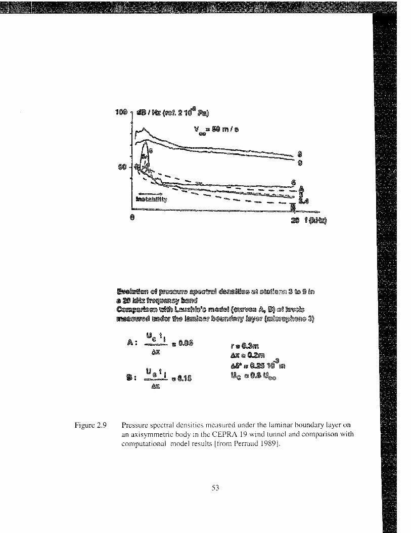
HPHI
Erotefai ®f pn*©»® ^p#sfesl äH䧮» at ®tetla@3 3 to S 1B
MummmS wn4w tit® tataar (tenttitfif &pr (Bl§f@pfisM 3)
Figure 2.9 Pressure spectral densities measured under the laminar boundary layer on an axisymmetric body in the CEPRA 19 wind tunnel and comparison with computational model results [from Perraud 1989].
53
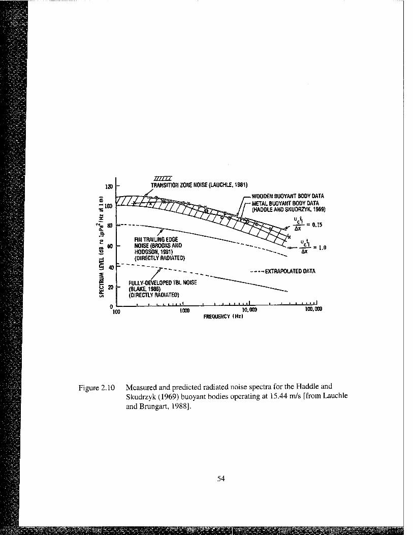
120
■100
HULL TRANSITION ZONE NOISE (LAUCHLE, 1981)
60
WOODEN BUOYANT BODY DATA METAL BUOYANT BODY DATA (HADDLE AND SKUDRZYK, 1989)
0.15
RNTRAIUN6EDGE NOISE (BROOKS WD HODSSON, 1981) (DIRECTLY RADIATED)
1.0
7' — EXTRAPOLATED DATA
20 FULLY-DEVELOPED TBL NOISE (BLAKE, 1986) (DIRECTLY RADIATED)
» » i i i 11 11 -i I,I i »»I 1000 10.0(H) 100,000
FREQUENCY (HzI
Figure 2.10 Measured and predicted radiated noise spectra for the Haddle and Skudrzyk (1969) buoyant bodies operating at 15.44 m/s [from Lauchle and Brungart, 1988].
54
CHAPTER 3
MODEL REFINEMENTS
A major objective of this research program is to continue to develop refinements
to the radiated noise models for transition noise. These theoretical extensions proposed
are necessary to complete the area of investigation of transition zone acoustics in a zero
pressure gradient. As discussed previously, there are two major approaches which can be
summarized in Figure 3.1. Lauchle began with a Lighthill acoustic analogy and moved to
a Liepmann analogy while Sornette and Lagier pursued a more rigorous Lighthill
approach. These are indicated by the top and bottom boxes in the figure. The right hand
box represents the use of the theoretical space-time correlation function whose form was
estimated using phenomenological assumptions. Lauchle (1981), Lagier and Sornette
(1986), and Audet, et al. (1989) used this form to make estimates of radiated noise
spectra. Similarly, the left hand box represents the semi-empirical form developed by
Josserand and Lauchle (1990). The dashed line between the two correlation functions
indicates an attempt to derive the constants of the theoretical function from the empirical
function. The lines and dates linking the models to the correlation function form boxes
indicating when certain modifications were made to the models as they were carried
toward validation with measured spectra. The following sections describe some of the
further refinements and analysis that are being performed. In order to satisfy the input
requirements for both models, it has been necessary to review previous fluid dynamic
55
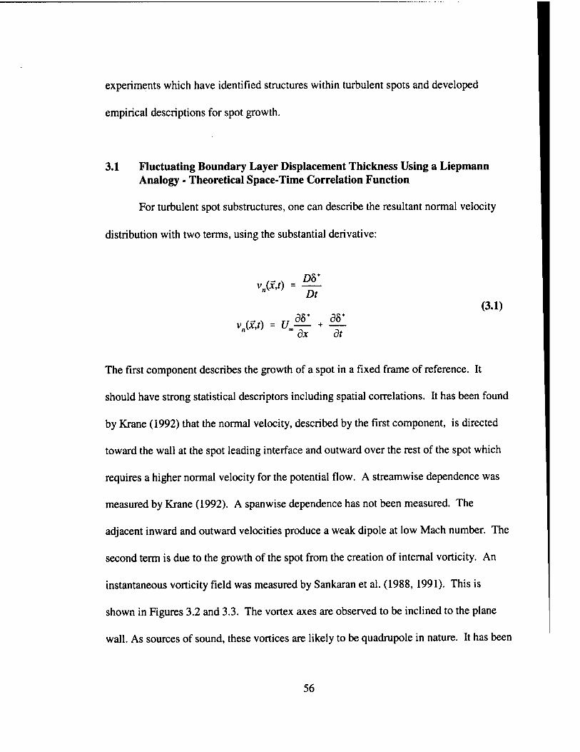
experiments which have identified structures within turbulent spots and developed
empirical descriptions for spot growth.
3.1 Fluctuating Boundary Layer Displacement Thickness Using a Liepmann Analogy • Theoretical Space-Time Correlation Function
For turbulent spot substructures, one can describe the resultant normal velocity
distribution with two terms, using the substantial derivative:
v.&O D8* Dt
/-^\ TT 38* c?8* v(x,t) = U + " " dx dt
(3.1)
The first component describes the growth of a spot in a fixed frame of reference. It
should have strong statistical descriptors including spatial correlations. It has been found
by Krane (1992) that the normal velocity, described by the first component, is directed
toward the wall at the spot leading interface and outward over the rest of the spot which
requires a higher normal velocity for the potential flow. A streamwise dependence was
measured by Krane (1992). A span wise dependence has not been measured. The
adjacent inward and outward velocities produce a weak dipole at low Mach number. The
second term is due to the growth of the spot from the creation of internal vorticity. An
instantaneous vorticity field was measured by Sankaran et al. (1988,1991). This is
shown in Figures 3.2 and 3.3. The vortex axes are observed to be inclined to the plane
wall. As sources of sound, these vortices are likely to be quadrupole in nature. It has been
56
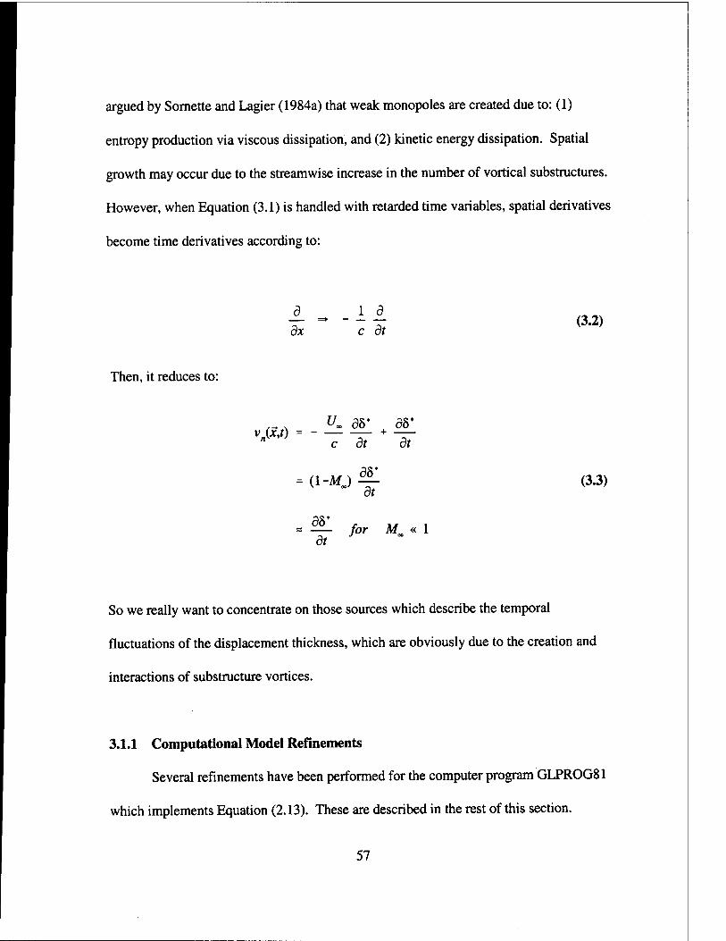
argued by Sornette and Lagier (1984a) that weak monopoles are created due to: (1)
entropy production via viscous dissipation, and (2) kinetic energy dissipation. Spatial
growth may occur due to the streamwise increase in the number of vortical substructures.
However, when Equation (3.1) is handled with retarded time variables, spatial derivatives
become time derivatives according to:
_a_ dx c dt
(3.2)
Then, it reduces to:
v(x,t) = - + " c dt dt
d-MJ ar dt
ar dt
for M„ « 1
(3.3)
So we really want to concentrate on those sources which describe the temporal
fluctuations of the displacement thickness, which are obviously due to the creation and
interactions of substructure vortices.
3.1.1 Computational Model Refinements
Several refinements have been performed for the computer program GLPROG81
which implements Equation (2.13). These are described in the rest of this section.
57
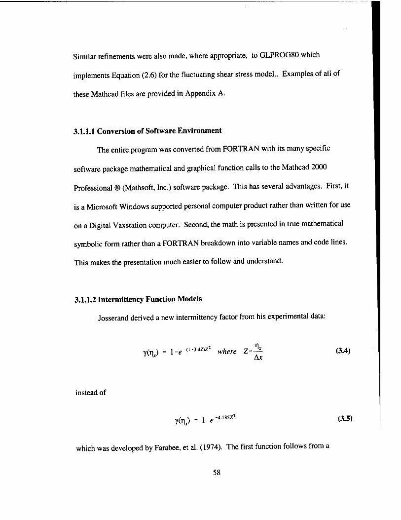
Similar refinements were also made, where appropriate, to GLPROG80 which
implements Equation (2.6) for the fluctuating shear stress model.. Examples of all of
these Mathcad files are provided in Appendix A.
3.1.1.1 Conversion of Software Environment
The entire program was converted from FORTRAN with its many specific
software package mathematical and graphical function calls to the Mathcad 2000
Professional ® (Mathsoft, Inc.) software package. This has several advantages. First, it
is a Microsoft Windows supported personal computer product rather than written for use
on a Digital Vaxstation computer. Second, the math is presented in true mathematical
symbolic form rather than a FORTRAN breakdown into variable names and code lines.
This makes the presentation much easier to follow and understand.
3.1.1.2 Intermittency Function Models
Josserand derived a new intermittency factor from his experimental data:
Y(n) = i-e(1+3-4Z>z2 where Z=
Ax (3.4)
instead of
Y(TO = l-e -4.185Z2 (3.5)
which was developed by Farabee, et al. (1974). The first function follows from a
58

formulation developed by Gedney (1979) (and Gedney and Leehey, 1989) for a combined
Dirac line source and constant source hypothesis. The comparison of these two relations
is shown in Figure 3.4. The Farabee relation is seen to have its highest slope earlier in the
transition zone. This carries through to modest increases in the predicted amplitudes as
well. The Josserand model predicts intermittencies that agree with experimental data
better than the Farabee model..
3.1.1.3 Burst Frequency Models
A new spot burst frequency description was also derived by Josserand (1986) based on
the Gedney (1979) hypothesis mentioned in Section 3.1.1.2:
u„ N(Z) = 2.38 (-2.)
Ax > [1-Y(ZJ] ln[- 1
1-Y(ZJ ] (3.6)
instead of
N(Z) = 1.272 (-^) Zr <T4185(Z*)2
Ax (3.7)
due to Farabee, et al. (1974). Josserand modified the constant in Equation (3.6) to yield a
better match with his experimental data. Note that Equation (3.6) can be evaluated with
the intermittency function described by either Equation (3.4) or (3.5). A comparison of
these three formulations is shown as a normalized burst rate, B(Z) (where N(ZX) is
multiplied by uJAx), in Figure 3.5. It can be seen that the magnitudes of the peak burst
59
rate for the Josserand function variants are about 4 time larger than that for the Farabee
model. The non-zero values of B(Z) predicted by Equation (3.6) beyond the end of the
transition zone seem physically unrealistic.
Of course, our real interest is in how the use of these different relations will affect
the calculation of the radiated noise. The results of these combinations of substitutions of
intermittency and burst rate are shown for one case in Figure 3.6. The measured data
come from a pressure sensor flush mounted in the laminar flow region on a body of
revolution in the CEPRA 19 wind tunnel (Perraud 1989). The parameters for that test
affecting the computational model inputs for GLPROG81 are listed in the caption. The
normalized rise time of 0.15 was suggested by Perraud. This new spot burst frequency
description results in a 6 to 8 dB increase in predicted radiated noise over much of the
frequency range of interest. The impact of a change of the intermittency model is
negligible compared to that of the burst rate. The Farabee form (Equation 3.7) of the
burst frequency function results in a slightly lower peak frequency as well and a larger
sound pressure magnitude below 50 Hz.
However, because Josserand (1986) reported a variance of 20% on his calculated
burst rate, which makes his empirical fit somewhat questionable, it seems likely that a
portion of the predicted high levels of sound are due to this over-prediction of the burst
rate.
3.1.1.4 Application of Strip Analysis
Multiplication of the result of Equation (2.13) by the transverse width of the
60
transition zone, W, yields the total radiated spectral pressure from the transition zone.
This assumes limited spanwise spot interaction which leads to homogeneity.
3.1.2 Incorporation of Measured Normal Velocity Fluctuations
Lauchle's assumed monopole description of the normal velocity in GLPROG81
has a provision for substitution of the normal velocity resulting from the water channel
measurements of Krane (1992). He measured the normal velocity using a mass flux
deficit to describe the displacement thickness (Figure 3.7). The velocity profile
measurement technique was developed by Bruneau and Pauley (1992,1995). This
technique tends to average out the time dependent fluctuations of 58*, but it does reveal a
negative mass flow deficit combined with the previously assumed (by Lauchle, 1981)
positive one. Krane identified the streamwise dependence with a weak dipole which
results from the negative normal velocity near the leading edge (overhang) of the
turbulent spot and a positive velocity associated with the passing of the rest of the spot.
The multipole source distribution proposed by Krane is shown in Figure 3.8.
Krane and Pauley (1993) also found that the interaction of two turbulent spots had
a minimal effect on the mass flux deficit (displacement thickness) and, therefore, the
normal velocity descriptor. This would imply that their normal velocity model should
apply to even a natural transition case. For both the single and the interacting spots, a
dependence on Zx was measured. A function was fit to this data,
TK(Z) = 0.30-exp[-1.45 - 3(Zf] (3.8)
61
This function is shown compared to Krane's measurements in Figure 3.9.
The dipole source shown in Krane (1992, Figure 5.1) was used to replace the
monopole source in GLPROG81. The proposed quadrupole sources were not included
because of their reduced radiation efficiency compared to the dipole and they do not
appear prominent for all velocities shown by Krane. However, the amplitude of the
normal velocity appears to be equal for the positive and negative events and was assumed
to be the same as the positive event modeled by Lauchle. Therefore, the dipole was
modeled (as shown in Pierce (1981, pp.170) as modifying the monopole pressure by the
factor of 2 sin[(fc d cos0)/2] where d is the separation distance of the two sources that
make up the dipole and the observation distance, r» d. This can be further simplified
for kd«l, to k d cosG. This would be appropriate for the low frequencies for which
transition noise seems important. The limitation in using this in the model is that it
would result in and amplitude independent of frequency at higher frequencies.
The separation distance can be modeled as 2 uc tj which is then equivalent to
d(Z) = 2 AJC TK(Z) * d = 0.4 Ax. S0GLPROG8I could be modified by multiplying
the previous result by 4 sin2[(0.2 k Ax cos0)] . However, if the separation distance
between the two dipole sources is taken to be a random variable, then the mean value of
the pressure spectrum is given by
G<f)) = M G_opo/e = E\Ad')} Gmono^ (3.9)
where Gmonopole is given by Equation 2.13 with the assumption of spanwise homogeneity.
62
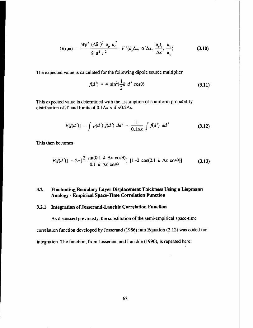
G(r,to) = Wp2 (A8*)2 u0 u'e
S^r2 F*(kAx, a*Ax, -^, —)
Ax u„ (3.10)
The expected value is calculated for the following dipole source multiplier
fid) =4 sin\-k d' cos6) (3.11)
This expected value is determined with the assumption of a uniform probability distribution of d' and limits of 0.1 Ax < d'<0.2Ax.
md)] = / P(d) fd) dd> = —L- f Ad) dd> (3.12)
This then becomes
r-r^j/M "i r2 sin(0.1 k Ax cosG), ri ^ /r. , , A m, E\fd )] = 2+[ -] [1-2 cos(0.1 & Ax cosG)] 0.1 k Ax cosG
(3.13)
3.2 Fluctuating Boundary Layer Displacement Thickness Using a Liepmann Analogy - Empirical Space-Time Correlation Function
3.2.1 Integration of Josserand-Lauchle Correlation Function
As discussed previously, the substitution of the semi-empirical space-time
correlation function developed by Josserand (1986) into Equation (2.12) was coded for
integration. The function, from Josserand and Lauchle (1990), is repeated here:
63
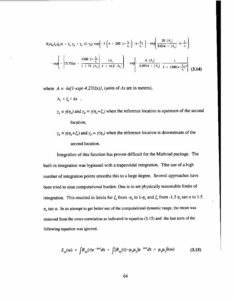
RfinAA.1) = iu id+ Y„ o-Yrf) exp{-5 ( 4+200 |T--2.| It "M exp 20 I A.
0.014 + |Ar
It-il
exp - 1260 IT—^-1
15.75A* 1 + 71 |A, 1 + 14.2 I A,
exp A I A.
0.0014 + |AJ j + ,300|T-^I2
(3.14)
where A = -ln[l-exp(-4.27/Ax)], (units of Ax are in meters),
A. = $, / Ax ,
yu = y(tjx) and yd = y(tix+£x) when the reference location is upstream of the second
location,
yu = y(rjx+£J and yd - y(rjx) when the reference location is downstream of the
second location.
Integration of this function has proven difficult for the Mathcad package. The
built-in integration was bypassed with a trapezoidal integration. Tthe use of a high
number of integration points smooths this to a large degree. Several approaches have
been tried to ease computational burden. One is to set physically reasonable limits of
integration. This resulted in limits for & from -r\x to \-r\x and £ from -1.5 r\x tan a to 1.5
t]x tan a. In an attempt to get better use of the computational dynamic range, the mean was
removed from the cross-correlation as indicated in equation (3.15) and the last term of the
following equation was ignored.
•M<°) - [R^e-^dx = {[R^-fijiJe-""* + HJiym) (3.15)
64
Because of the difficulty in integrating the Josserand (1986) form of the space-
time correlation function, an effort was made to look for simplification of the function to
make integration easier. However, it does not appear that this function has a form that is
direction separable for x and z.
3.2.2 Chase Statistical Modification
Chase (1989) has suggested that the first exponent term in Equation (3.14) can be
replaced by a more general term based on the probability of state transition to turbulence
of form:
exp' N;
ix-^l fy (i-T^f) "c
(3.16)
However, Josserand found that both terms predict the measured correlation values well
for 0.3^0.7; but, that outside of these limits, the Chase theoretical term tended to over-
predict the correlation. Both terms are available as options in the computational software.
Limit evaluation has determined that the Chase modification to the Josserand-Lauchle
correlation function does not improve the results in comparison to measured data for
natural transition. A comparison of the Josserand and the Chase modified correlation
surfaces over the transition zone is shown in Figure 3.10. The differences are subtle with
the Chase term having deeper troughs in the amplitude surface.
65
3.3 Two Fluids Model with Refined Normal Velocity
In tying together all the approaches, the Audet and Sornette-Lagier approaches did
not provide any advances because of simplifying assumptions to allow integration and
heavy dependence on Lauchle's (1981) functions. The refined normal velocity description
could be substituted into the two fluids model but it would not provide an advantage over
the refined fluctuating displacement thickness model. Knowledge gained of the radiated
noise component magnitude can be used to further refine the two-fluids model of Audet,
et al. (1989b) for wall pressure fluctuations as input to the fluid-structure interaction
problems of interest.
Their predictions used simplifying assumptions for their more general equation.
The retarded time in the equation does not take into account the separation distance in the
2 point correlation. It accounts only for the reference point. Global stationarity is
assumed. No spot interaction is assumed. All values are taken for rj=Q. Spatial '
dependence is separated from temporal dependence.
The good comparison of the Lauchle (1981) model with CEPRA wind tunnel
data when using normalized rise times of 0.05 to 0.15 must be viewed with reserve since
the authors indicated that some data were contaminated by corner vortex growth
overlapping the sensor locations.
3.4 Accounting for Vortical Motions
Another objective of this study is to investigate the feasibility of incorporation of
effects due to vorticity into either of Lauchle's models. This will mainly draw upon the
66
prior work of Powell (1995), Hardin (1991), Lund (1989), and the many papers of Kambe
and Obermeier. Williams, Fasel, and Hama (1984) also made a great experimental
contribution with their mapping of the three-dimensional vorticity field in boundary layer
transition. It is anticipated that this would form a second source term in the fluctuating
displacement thickness model in a manner similar to the S and S0 functions of Lagier and
Sornette (1986). Lagier and Sornette concluded that the contribution of a shear interface
at the edge of a turbulent spot (due in large measure to the presence of these vortices) was
insignificant compared to the overall growth of the spot.
Sankaran, Sokolov, and Antonia. (1988) and Sankaran, Antonia, Bisset, and
Sokolov (1991) used instantaneous velocity field measurements to identify a
superposition of vortex sources within a turbulent spot. The existence of vorticity
formations may help explain the Uj$noise dependence by looking at the sources as
primarily quadrupoles with some monopole like bursting. The measurements indicate
that the spatial growth of the spot is directly related to a streamwise increase in the
number of substructures. Substructures are generally created near the trailing edge of a
spot, and all convect at the same velocity 0.8 U„. This means that the cumulative
contribution from these substructures will be greatest near the midpoint of the transition
zone because the number of spots is greatest there. Would incorporation of a distribution
of these vortices help account for the highly spatially dependent normal velocity
component due to db*/dtl Many would argue that the hydrodynamic fluctuations due to
these substructures is statistically the same as what would be found with a fully turbulent
67
boundary layer however, the spatial and temporal extent is limited by the axial
dependence of intermittency and the burst rate. Hence, the vortical contribution is
captured in the use of TBL statistics in models such as Howe's. Therefore, no additional
changes are made to any of the models since they either utilize the modified TBL
statistics or not.
3.5 Incorporation of Green's Function for Transition Zone Near Half-Plane Leading Edge
Howe's model as described in section 2.6.1 has been implemented in a Mathcad
worksheet, MSHTRANS99, that is provided in Appendix A.4.
The trick on the integration of Equation (2.25) is to apply a window function that
varies with frequency. A longer window is required for low frequencies and a short
window is required for high frequencies. Also, to avoid aliasing, a much higher sampling
rate is necessary for high frequencies than for the low frequencies. Trapezoidal
integration is also used rather than the Mathcad built-in function.
Howe's original formulation uses the intermittency function shown in Equation
(3.5). An alternative Mathcad worksheet uses the Josserand intermittency function
(Equation 3.4). The impact is about a 4 dB decrease in the radiated pressure levels with
the Josserand intermittency function.
An alternative use of the formulation provided by Howe would be to substitute the
pressure spectrum for the wall pressures as determined by Josserand (1986) rather than
intermittency modified Chase (1980) description of TBL wall pressures for the section of
68
the finite thickness half-plane (hydrofoil) surface S covering the transition zone. This has
not yet been pursued.
69
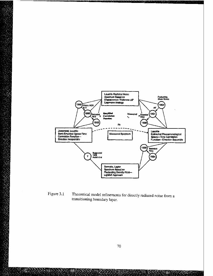
Leuchte RaSstsd Moäaa Spedtum Basad on DiaplaoBfnsnS TWeiinses /IS* Uajwsnn AnaSogy
SomsRo, Lagicf SpscGurn Bsssd ert Ruduölng DsraSSy ffea—
Spaes—Tims CeroSötaii Fuitetlen—DSwetien Sepm&äs
Figure 3.1 Theoretical model refinements for directly radiated noise from a transitioning boundary layer.
70
aaa
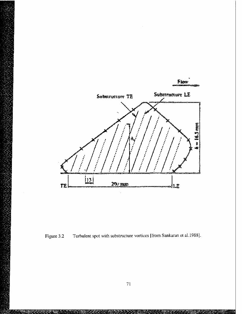
Figure 3.2 Turbulent spot with substructure vortices [from Sankaran et al.1988].
71
»Um M£M&MMäi£M^^äMsE Ü^Ü^ÜÜ nfSStv illOi
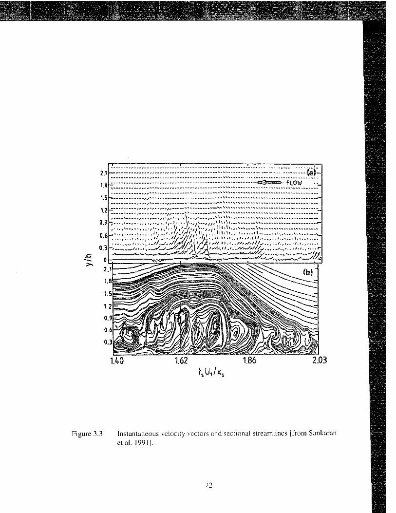
2.1
1.:
1.5
1.2
0.9-
0.6-
0.3
■ -(a)—
FLOW
'//' •//•
,». » •
^*-,--v—^—"-tv^
Figure 3.3 Instantaneous velocity vectors and sectional streamlines [from Sankaran etal. 19911.
72

2^ YFsrabssCZ) := 1 - exp\-4.185Z j
yJUZ) := I - exp[-(l -t- 3.4Z)Z2]
Empiiteai relafions from Farabaa, at al. (1974).
Empirical relattons from Jossarartd snd Lauchle (1986) which was bas®d on the work of Gsdnsy (1879) asessing both a Direc tin® sourc® hypoths» and a consent sourc© hypothecs for intermitency,
Figure 3.4 Comparison of empirically derived intermittency functions.
73
m *^m^ IMg^äwgiiSgfc£^gigigl MM&IMs&m,* >S7Ms^^^^i^k
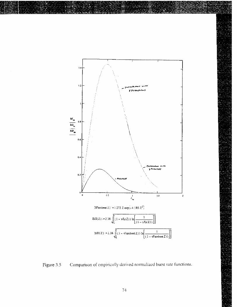
*WM
ail
BJF
TsSirf*0
T 3*0 ft&i/^ä*^
BFarabee<Z) := 1 272Zi-xp\-4.185-Z2)
BJJ(Z):=2.38- j (1 - rJL(Z))-ln (1-7JUZ))
BJF(Z) : = 2.38 (1 - rFsrubss(Z))'ln I
(1 - yfarmbc^Z))
Figure 3.5 Comparison of empirically derived normalized burst rate functions.
74
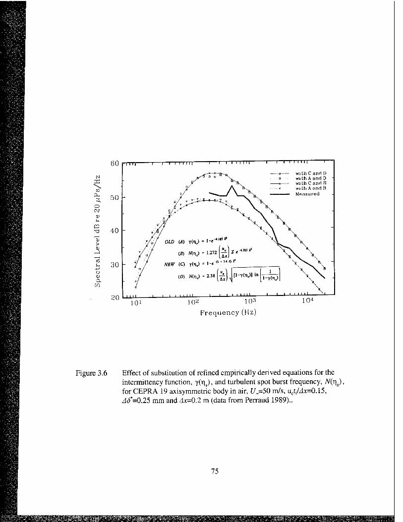
60 p Ml 1 1 I I I Mil 1 1 I I I I Ml
N K
(Ö
a. 50 o <M cu I-,
m -d 4U ,—t
V > V
_1 ^~i
<a S-, HO ->-> o <v a,
en
20
i i i iiii
Frequency (Hz)
Figure 3.6 Effect of substitution of refined empirically derived equations for the intermittency function, 7(1^), and turbulent spot burst frequency, N(r\x), for CEPRA 19 axisymmetric body in air, Uj=50 m/s, ucti/Ax=0A5, Aö*=0.25 mm and JJC=0.2 m (data from Perraud 1989)..
75
^^m^^^^^^^^^Mmmmidm^^^^^mSi!^^^ä^^^^m^mj^i^^ sss^EÄ
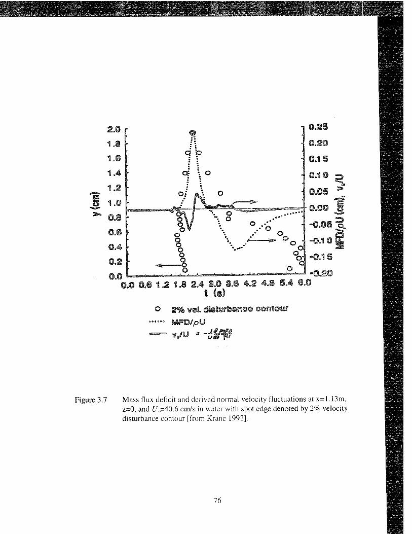
wm
O g^ * s e c so
Figure 3.7 Mass flux deficit and derived normal velocity fluctuations at x= 1.13m, z=0, and U=40.6 cm/s in water with spot edge denoted by 2% velocity disturbance contour [from Krane 1992].
76
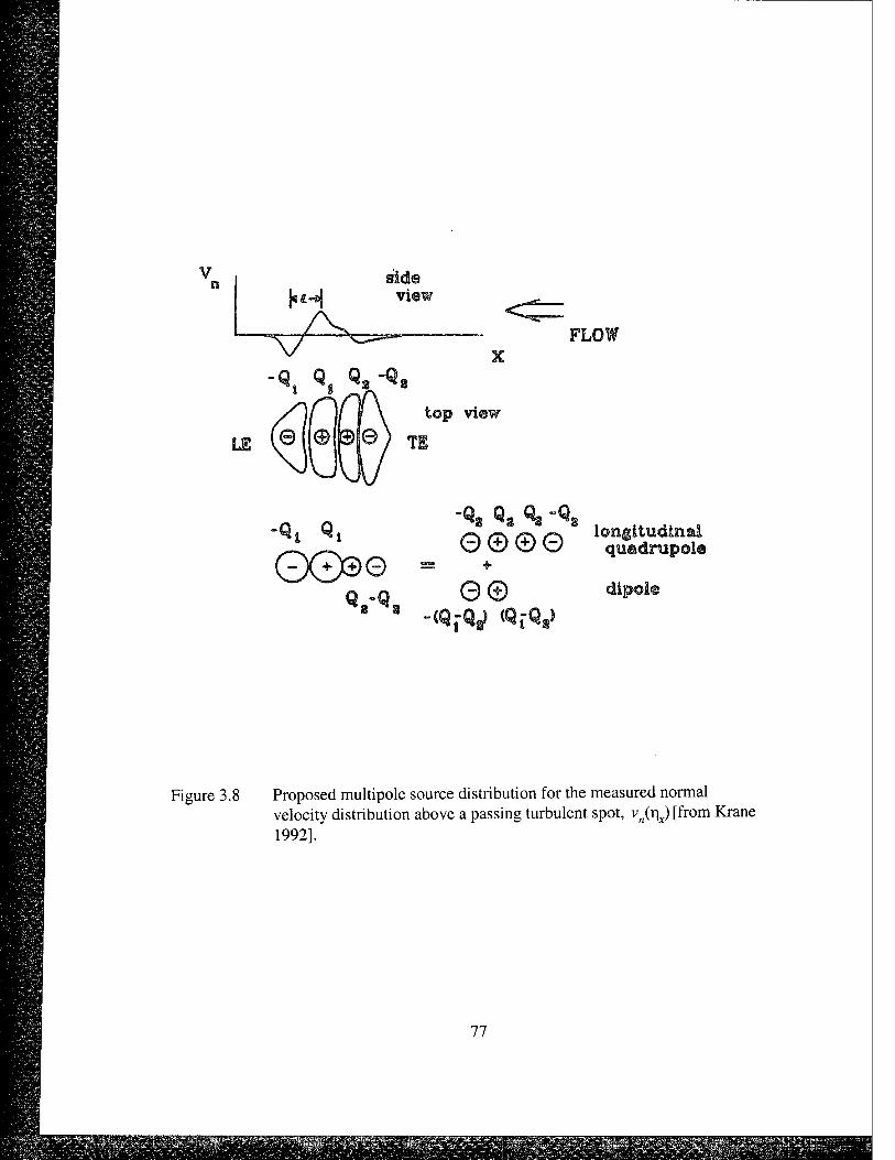
n
•4 ^1
O000 V«,
v£/ V3/ <C/ quadnipol«
e© e
Figure 3.8 Proposed multipole source distribution for the measured normal velocity distribution above a passing turbulent spot, v^rQ [from Krane 1992].
77
MPP mm

u0.0^o.o5
A z,Z Normalized Transition Zone Coord, Z
Krane Data Function Fit
Figure 3.9 Comparison of Krane (1992) measured non-dimensional rise time, \ictJAx, and function TK(ZX) fit to the data.
78

Variation with x and £,z with ^x=1.0.
Variation with E,x and £,z with x=0.
Josserand correlation
Figure 3.10 Comparison of correlation surface, R,(r|x,^x,0,t), for empirical
space-time correlation function for original Josserand form and Chasefirst exponential term statistical modification for U=11.8 m/s, Ax=1.83m, with r|x/Ax=0.50.
79
CHAPTER 4
RADIATED SOUND POWER PREDICTIONS
4.1 Model Comparisons
The three transition noise models based on Lauchle's theoretical space-time
correlation function were each exercised to predict far field radiated noise from natural
transition a flat plate with zero pressure gradient with seven velocities for air flows and
seven velocities for water flows in appropriate ranges. The model which required the
integration of the Josserand empirical space-time correlation function was run for selected
conditions for comparison to the other models. The higher frequency results for that
model are not considered to be appropriate yet. The Mathcad worksheets for these
models are all provided in Appendix A:
GLPROG80.MCD (implementing Equation 2.6, Appendix A.l),
(G. Lauchle PROGram 1980)
GLPROG81.MCD (implementing Equation 2.13, Appendix A.2),
(G. Lauchle PROGram 1981)
KMTRANS00.MCD (implementing section 3.1.2, Appendix A.3),
(Krane, Marboe TRAnsition NoiSe 2000)
JLTRANS99.MCD (implementing Equations 2.12 with 2.15, Appendix A.4), and
(Josserand, Lauchle TRAnsition NoiSe 1999)
80
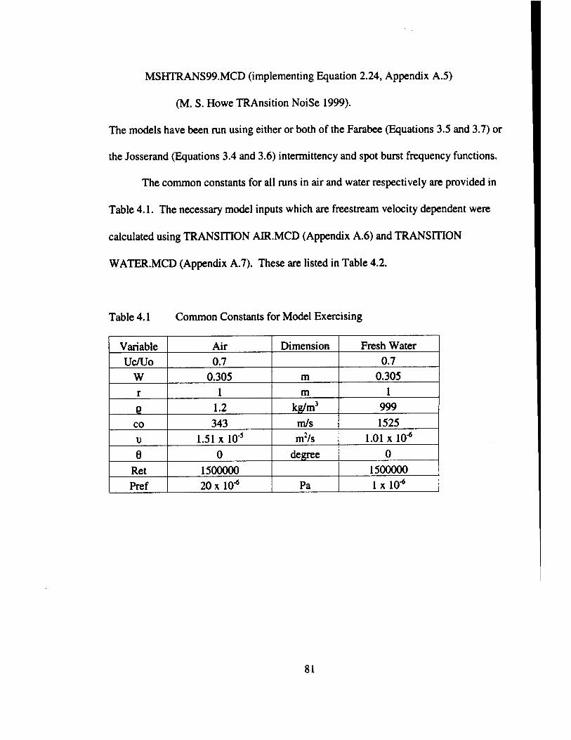
MSHTRANS99.MCD (implementing Equation 2.24, Appendix A.5)
(M. S. Howe TRAnsition NoiSe 1999).
The models have been run using either or both of the Farabee (Equations 3.5 and 3.7) or
the Josserand (Equations 3.4 and 3.6) intermittency and spot burst frequency functions.
The common constants for all runs in air and water respectively are provided in
Table 4.1. The necessary model inputs which are freestream velocity dependent were
calculated using TRANSITION AIR.MCD (Appendix A.6) and TRANSITION
WATER.MCD (Appendix A.7). These are listed in Table 4.2.
Table 4.1 Common Constants for Model Exercising
Variable Air Dimension Fresh Water
Uc/Uo 0.7 0.7
W 0.305 m 0.305
r 1 m 1
Q 1.2 kg/m3 999
CO 343 m/s 1525
u 1.51 x 10⁻⁵ m2/s 1.01 x 10"6
0 0 degree 0
Ret 1500000 1500000
Pref 20 x 10^ Pa lxlO-6
81
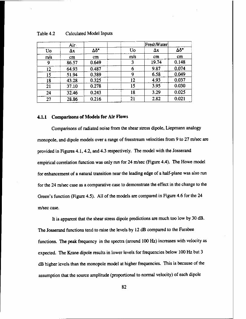
Table 4.2 Calculated Model Inputs
Air FreshWater Uo Ax A6* Uo Ax A6* m/s cm cm m/s cm cm 9 86.57 0.649 3 19.74 0.148 12 64.93 0.487 6 9.87 0.074 15 51.94 0.389 9 6.58 0.049 18 43.28 0.325 12 4.93 0.037 21 37.10 0.278 15 3.95 0.030 24 32.46 0.243 18 3.29 0.025 27 28.86 0.216 21 2.82 0.021
4.1.1 Comparisons of Models for Air Flows
Comparisons of radiated noise from the shear stress dipole, Liepmann analogy
monopole, and dipole models over a range of freestream velocities from 9 to 27 m/sec are
provided in Figures 4.1,4.2, and 4.3 respectively. The model with the Josserand
empirical correlation function was only run for 24 m/sec (Figure 4.4). The Howe model
for enhancement of a natural transition near the leading edge of a half-plane was also run
for the 24 m/sec case as a comparative case to demonstrate the effect in the change to the
Green's function (Figure 4.5). All of the models are compared in Figure 4.6 for the 24
m/sec case.
It is apparent that the shear stress dipole predictions are much too low by 30 dB.
The Josserand functions tend to raise the levels by 12 dB compared to the Farabee
functions. The peak frequency in the spectra (around 100 Hz) increases with velocity as
expected. The Krane dipole results in lower levels for frequencies below 100 Hz but 3
dB higher levels than the monopole model at higher frequencies. This is because of the
assumption that the source amplitude (proportional to normal velocity) of each dipole
82
source is the same as for the monopole, compactness, and an assumed uniform
distribution of dipole separation distances [d = 2 uct = 2 Ax (uct/Ax)]. This tends to
smooth out the nulls associated with the sine function.
4.1.2 Comparisons of Models for Water Flows
Comparisons of radiated noise from the shear stress dipole, Liepmann analogy
monopole, and dipole models over a range of freestream velocities from 9 to 27 m/sec are
provided in Figures 4.7,4.8, and 4.9 respectively. The model with the Josserand
empirical correlation function was only run for 24 m/sec (Figure 4.10). The Howe model
for enhancement of a natural transition near the leading edge of a half-plane was also run
for the 24 m/sec case as a comparative case to demonstrate the effect in the change to the
Green;s function (Figure 4.11). All of the models are compared in Figure 4.12 for the 24
m/sec case.
The comparative results are similar to those seen in for the airflow cases but are
45 to 55 dB higher (after accounting for 26 dB difference in reference pressures) for the
same freestream velocity.
4.2 Role of Rise Time, t,
With a factor of lit2 in the amplitude coefficient of the power spectrum, the
nondimensional rise time, ujt/Ax, (where t, is defined in Figure 1.5) has usually been an
independent parameter whose value is chosen to get the model results to match the
experimental data. It has taken on many values from 0.05 to the physically implausible
83
1.36. This parameter is difficult to measure and would seem to be quite dependent on the
pressure gradient. However, it is useful to look at some values which have been extracted
from various experimental investigations in order to make a reasonable first estimate for
use in the computational code. A delta wing generated vortex as seen in Emmons spots
produced by Littell and Eaton (1991) yielded a nondimensional rise time of 0.05. Use of
data from Huang and Shen (1989) gave u,s/Ax=0.lSl. Other recent investigations on a
flat plate showed a value of 0.30. As mentioned previously, Perraud (1989) found best
agreement for Q.Q5<u(t/Ax<Q.\5. Audet et al. (1989) used a value of 1.36 which
indicates normal velocity fluctuations continues even after the flow is fully turbulent.
Lauchle (1981) found that 0.45 provided the best agreement with the Haddle and
Skudrzyk (1969) data. It appears that a band of values for uj/Ax around 0.20 will
provide a reasonable first estimate. Data from the experiments performed by Krane
(1992) in the fluid mechanics portion of the ONR project indicate that for an isolated
turbulent spot the rise time is 0.06<M,i, ni/dx<0.30 and non-dimensional fall time is
0.l3<ujifal/Ax<OJ4. Therefore, ujt/Ax - 0.20, was used for each of the models for the
comparison shown in Figure 4.13 for the airflow condition measured in the experiment
described in Chapters 5 and 6.
43 Effects of Pressure Gradient
It has become evident that transition zone noise production is quite dependent
upon the pressure gradient over the transition surface. Narasimha et al. (1984) and
Mautner (1985) found that a positive pressure gradient results in wall pressure fluctuation
84
spectral shape and amplitude very close to those for a zero pressure gradient case.
Mautner found that for an adverse pressure gradient that the nondimensional wall
pressure power spectrum stayed constant to a nondimensional frequency offS'/U=\
rather than rolling off as 1// after fi'/Uj=0.l. Mautner concluded that this broader
frequency forcing function would result in a greater wall pressure field coupling with
both the structure and the acoustic field to produce more intense near and far field noise
levels.
Huang and Shen (1989) found wall pressure levels 2 to 3 times higher for
transition in adverse pressure gradients compared to TBL wall pressure levels. Mautner
and Van Atta (1982) found rms wall pressures for individual turbulent spots to be 0.010-
0.015 of dynamic pressure (Vz pU02) for zero and favorable pressure gradients and 0.015-
0.030 of dynamic pressure in adverse gradients. More importantly, in the adverse
gradient, the wall pressure spectrum was nearly constant magnitude with increasing
frequency rather than the typical decreasing slope. This is enhanced further if transition is
induced by laminar boundary layer separation and re-attachment. In particular, Huang and
Shen found that wall pressures in reattachment zones for laminar separation were 10 to 15
times higher.
The models all have a sensitivity to the length of the transition zone and the
consequent decrease in the rise and fall time of the intermittency indicator function.
Favorable pressure gradients demonstrate similar or slower transition than a zero pressure
gradient. An adverse gradient will tend to accelerate transition and shorten the transition
zone and spot growth. Transition in an adverse pressure gradient will result in higher
85
radiated and structural excitation levels in comparison to transition in a zero pressure
gradient. It is also important to note that for adverse pressure gradients, it is very possible
that some amount of flow separation and re-attachment is contributing to the radiated
noise.
4.4 Effects of Scattering by a Plane Leading Edge
Howe's model shows the impact of the transition zone to be only at very low
frequencies (below about 200 Hz). The quadrupole noise normally associated with the
fully turbulent boundary dominates for higher frequencies in this model since it is not
restricted to the transition zone alone. The effect of using the Josserand intermittency
function is to decrease the radiated noise by about 4 dB (as shown in Appendix A.5).
This is because the intermittency is used to multiply the point pressure spectrum and the
Josserand levels are slightly lower for a given Z, than the Farabee derived function. In
the other models, it is the Josserand burst rate that accounts for the increased levels
calculated when the Josserand functions are used.
4.5 General Assessment of Models
The general applicability of the models described or treated in this dissertation are
assessed as follows:
Fluctuating Shear Stress Using a Lighthill Analogy (GLPROG80) - Predicted
noise levels are much too low (35 dB below other models). Even the use of the Josserand
intermittency and burst frequency functions only increases the results by 12 dB.
86
Fluctuating Displacement Thickness Using a Liepmann Analogy. Theoretical
Space-Time Correlation Function (GLPROG81) - The premise for the model assumes the
growth of a turbulent spot from a laminar displacement thickness height to a turbulent
height over a convection time in the transition zone. Based on the highest measured burst
rates of spots being between 25 % and 60% of the transition zone (Josserand 1986 and
Farabee et al., 1974), predictions have appeared to be best using a normalized rise time,
uct/Jx, of 0.5 to 1.0. Audet et al. claim a best fit with their measurements using
normalized rise time of 1.35 which is physically implausible. This is because the
monopole model of the sound source is not correct and a higher radiation efficiency is
modeled than appropriate. Thus, slower growth times must be used to compensate. This
is where the substitution of the dipole description of vn(t) yields a better model in that, at
low frequencies, it is kd cos 6 lower than the levels calculated in GLPROG81. The lower
efficiency dipole is necessary to allow the use of normalized rise times of 0.20 (or the
variation from 0.15 to 0.30 over the transition region) for individual spots measured by
Krane (1992) in an open water channel. This dipole is implemented in a variation of
GLPROG81 called KMTRANS00. For k d >1, the sound pressure level amplitudes
predicted by GLPROG81 and KMTRANSOO are within a few dB of each other because
of what appears to be two sources with constructive and destructive interference and a
smearing due to the range of d for the dipole description of all the spots in the transition
zone. The prediction by KMTRANSOO matched the measured spectral shape better for
frequencies greater than 200 Hz. The uncertainty in the angle of the dipole axis also has a
great effect on the amplitude of the prediction. The uncertainty in the measurement for
87
lower frequencies does not allow a meaningful comparison.
Fluctuating Displacement Thickness Using a Liepmann Analogy. Empirical
Space-Time Correlation Function (JLTRANS89) - This produces prediction levels
slightly higher in low frequencies than GLPROG81 but still does not compute well in
Mathcad. While it might provide a better empirical basis for modeling, it does not appear
to provide enough of an advantage over the simpler models for design.
Two-Fluids Model - Lagier and Sornette Formulation - This model has two source
terms. The first is modification of TBL source levels by multiplication with the
intermittency factor. In effect, this makes it a lesser source at higher frequencies than the
nearby (and covering a much greater spatial extent) fully developed turbulent boundary
layer. The second term is a radiated pressure from a monopole source based on a
Lighthill analogy that is effectively the same as the fluctuating baffled piston-like source
due to the Liepmann analogy used by Lauchle. Their formulation provides no real
improvement over GLPROG81, and is computationally more complex.
Boundary Laver Transition on Symmetric Hydrofoils - Howe Formulation
(MSHTRANS99) - This model highlights the effect of the scattering and diffraction from
a nearby leading edge on the low-frequency, flow-induced noise spectrum due to the
transition zone. No comparison can be made yet against wind tunnel or water tunnel
measurements. The spectrum derived from Josserand's empirical space-time correlation
function model (Lauchle and Park, 2000) could be substituted for the Chase spectrum
model for the calculations covering the transition zone. The impact of this substitution is
not known but is not expected to be large. The low frequency amplitudes may be low due
88
to only using the intermittency weighted Chase point pressure spectrum and not including
the acoustic pressures measured in this study and in wall pressures in a transition zone in
air measured by Dufourq (1984).
89
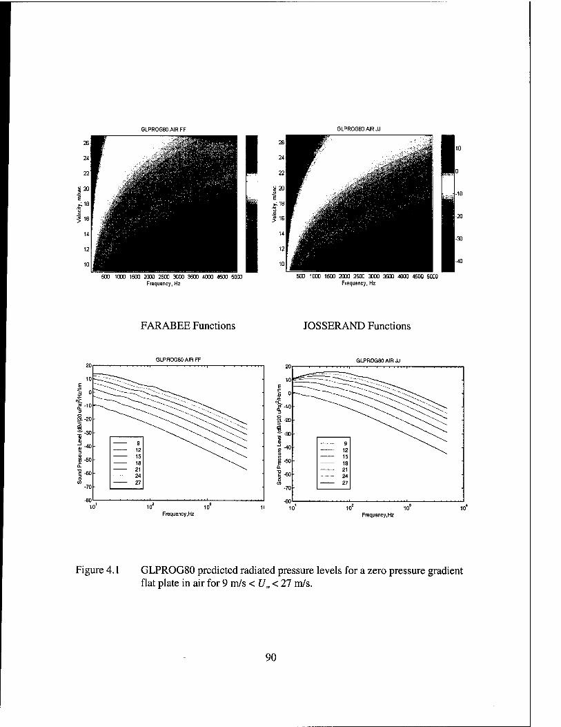
GLPROGBOAIRFF GLPROG80 AIR JJ
500 1000 1500 2000 2500 3000 3500 4000 4500 5000 Frequency, Hz
500 1000 1500 2000 2500 3000 3500 4000 4500 5000 Frequency, Hz
FARABEE Functions JOSSERAND Functions
GLPBOG80 AIR FF 20
101-
I 0[
i" -io - i
1-20 •
i r-30- i
\-AO- i
! -50-
: -60- i
-70-
-80 10'
GLPROG80 AIR JJ -f-r-n ■ ■—'—•-»
>$* -!^~- d; \^>-C^\-^^ ■
■~-~-~Z^\^^> ^T""""^^^ •
■
\^ ^" "^o- ■
9 12
15 16
21 24 27
?-10
r-30
g-40- « 8 -50 •
10 10 Frequency,Hz
-80 10'
,-fCS^22^ --C
^§§1^^ : ■ ^~v^ ^^\J^\T^\.
, q 12 15
' 18 ■
■ • 21 ■ 24 - 27
10 Frequency,Hz
Figure 4.1 GLPROG80 predicted radiated pressure levels for a zero pressure gradient flat plate in air for 9 m/s < U«, < 27 m/s.
90
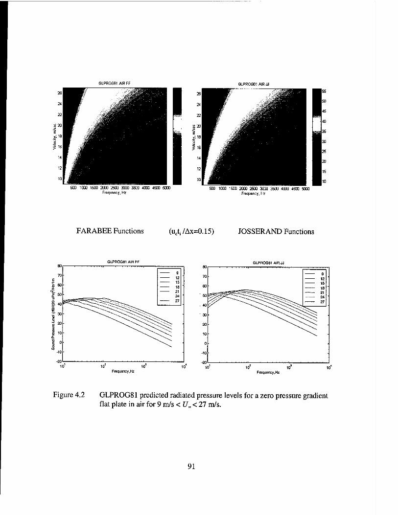
GLPR0G81 AIR FF
261 Ü
241 • ■!;,'v"f'j¥i^Si ^B
22 1 ,-^HI Ü2OH
1 ■ 11BB
' ' iM
ul
12»
1DI J
GLPR0G61 AIRJJ
500 1000 1500 2000 2500 3000 3500 4000 4500 5000 Frequency, Hz
500 1000 1500 2003 2500 3000 3500 4000 4500 Frequency, Hz
5000
FARABEE Functions (ucti/Ax=0.15) JOSSERAND Functions
GLPROG81 AIR FF GLPROG81 AIR JJ
Frequency,Hz 10 10
Frequency ,Hz
Figure 4.2 GLPROG81 predicted radiated pressure levels for a zero pressure gradient flat plate in air for 9 m/s < £/„ < 27 m/s.
91
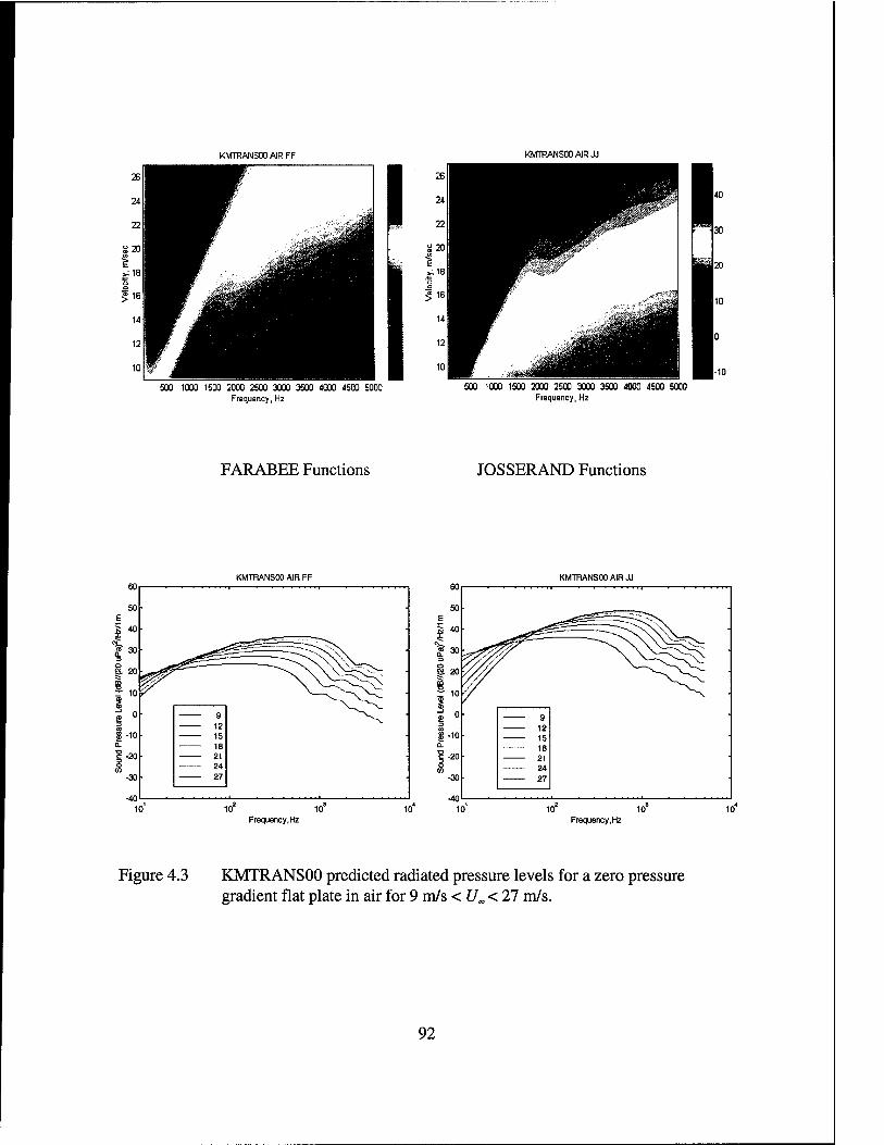
KMTRANSOO AIR FF KMTRANSOO AIR JJ
500 1000 1500 2000 2500 3000 3500 4000 4500 5000 Frequency, Hz
500 1000 1500 2000 2500 3000 3500 4000 4500 Frequency, Hz
5000
FARABEE Functions JOSSERAND Functions
KMTFiANSOO AIR FF KMTRANSOO AIR JJ
i o CO
| -10 a. |-20 o
9 12 15 18 21 24
-30 ■ 27
Frequency.Hz Frequency.Hz
Figure 4.3 KMTRANSOO predicted radiated pressure levels for a zero pressure gradient flat plate in air for 9 m/s <U„<21 m/s.
92
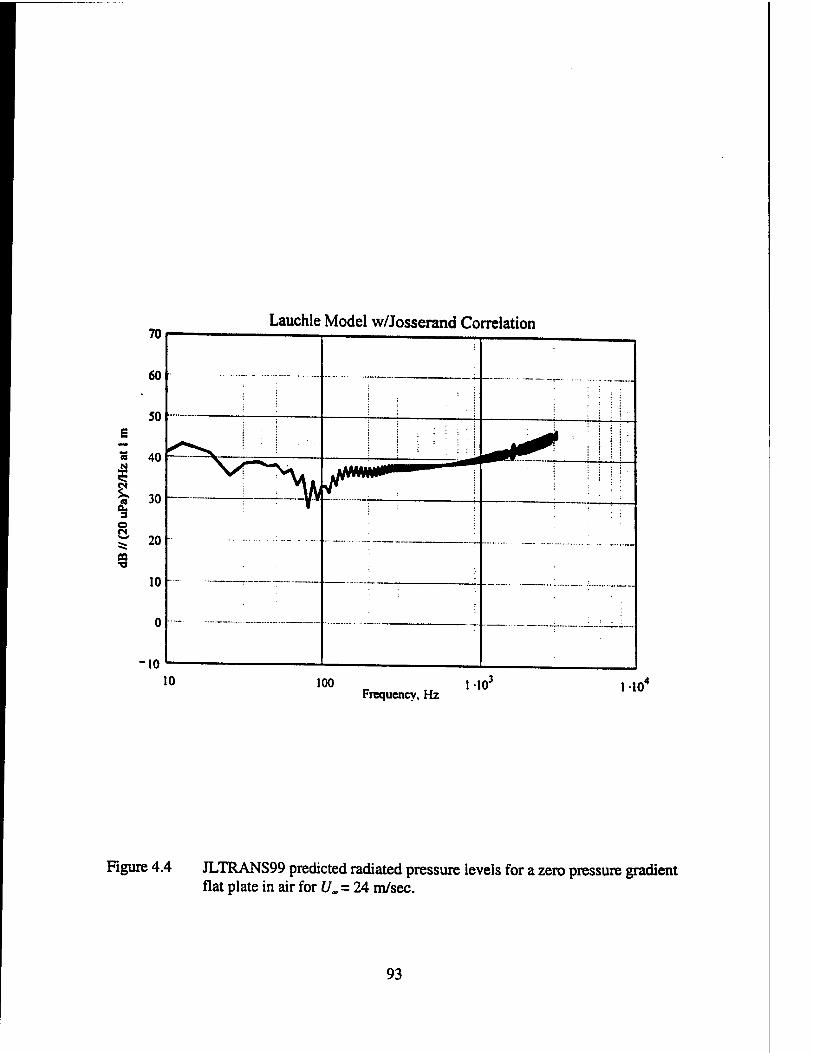
70
60
50 E
3 40
fc 30
o
CO
20
10
0
10
Lauchle Model w/Josserand Correlation
-
1 1 1 ! • ; • i
- :...-
- - — "• v
10 100 MO Frequency, Hz
3 1-HT
Figure 4.4 JLTRANS99 predicted radiated pressure levels for a zero pressure gradient flat plate in air for U„ = 24 m/sec.
93
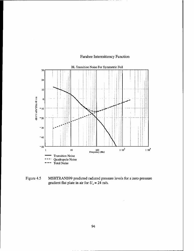
Farabee Intermittency Function
30
20
10
BL Transition Noise For Symmetric Foil
£ -io
€ -20
"30
"40
-50
iHsliiHl:!; ■■■■Ititil! ;^rTUMIT\M !"rUmi
I LLI-H' MM \ ! : »i* : i i I I \
--*■•■ ; : i : H - ■;!!!■■■!! 'A I ! I r ! i r
10
~~ Transition Noise """ Quadrupole Noise — Total Noise
100 Frequency (Hz)
110 110'
Figure 4.5 MSHTRANS99 predicted radiated pressure levels for a zero pressure gradient flat plate in air for U„ = 24 m/s.
94
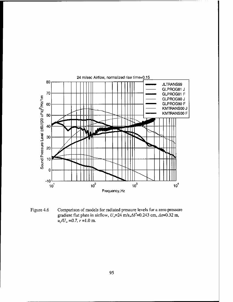
24 m/sec Airflow, normalized rise time=0.15 80
70
60
50
N X
CO Q.
O CM.
m 40
35 30
CO CO p
c o
CO
20
10
-10 10
JLTRANS99 GLPROG81 J
~-" GLPROG81 F GLPROG80 J GLPROG80 F KMTRANSOO J KMTRANSOO F ____
/
."?" Z-- ^iHII
) /} "" s-
/ '
10 10 10 Frequency,Hz
Figure 4.6 Comparison of models for radiated pressure levels for a zero pressure gradient flat plate in airflow, U=2A m/s^Jc5*=0.243 cm, Ax=Q32 m, u/U„=0.7, r=1.0m.
95
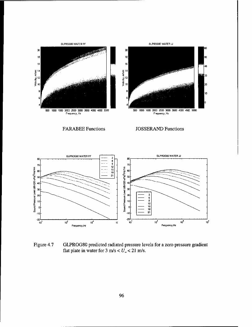
GLPROG80 WATER FF GLPROG80 WATER JJ
500 1000 1500 2000 2500 3000 350O 40O0 4500 5000 Frequency, Hz
500 1000 1500 2000 2500 3000 3500 40O0 4500 Frequency, Hz
5000
FARABEE Functions JOSSERAND Functions
80
70 E | 60
w" S. 60 O St 40
i» g 20 3 CO
| 10 Q.
1 o
-10-
-20
GLPROG80 WATER FF 3 6 9 12 15 ■ - 18 21
■ ■
•^^^—""^--^r^^O"'--^---^
^\.
■
GLPROG80 WATER JJ
10 10 Frequency.Hz Frequency,Hz
Figure 4.7 GLPROG80 predicted radiated pressure levels for a zero pressure gradient flat plate in water for 3 m/s < C/„< 21 m/s.
96
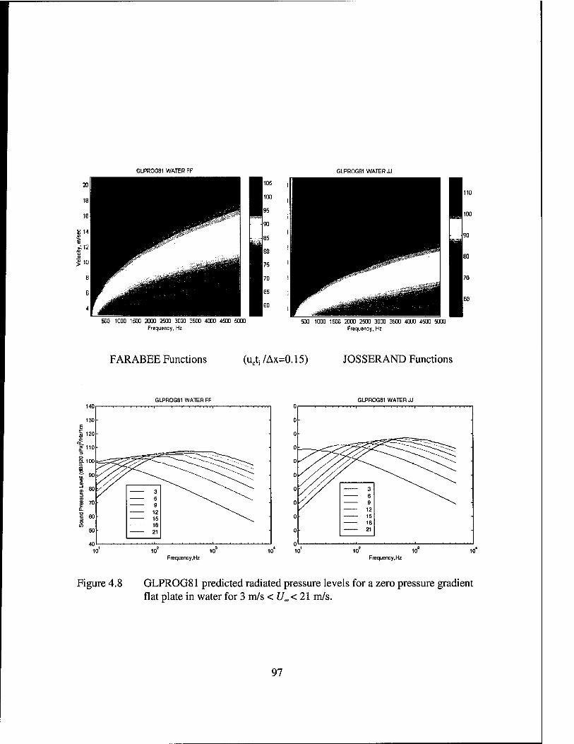
GLPR0GS1 WATER FF GLPR0GB1 WATER JJ ■ 105 |
1 100 1 95 SO
65
60 !
75 '
70 I
65 ;
60
500 1000 1500 2000 2500 3000 3500 4000 4500 5OO0 Frequency, Hz
500 1000 1500 2000 2500 3000 3500 4000 4500 5000 Frequency, Hz
FARABEE Functions (ucti/Ax=0.15) JOSSERAND Functions
GLPROG81 WATER FF GLPROG81 WATER JJ
Frequency.Hz 10 10
Frequency.Hz
Figure 4.8 GLPROG81 predicted radiated pressure levels for a zero pressure gradient flat plate in water for 3 m/s < U„ < 21 m/s.
97
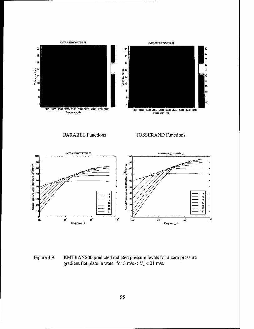
KMTRANSOO WATER FF KMTRANSOO WATER JJ
500 1000 1500 2000 2500 3000 3500 4000 4500 5000 Frequency, Hz
90
80
Ira BO
•50
40
30
20
10
0
-10
500 1000 1500 2000 25C0 3000 3500 4000 4500 5000 Frequency, Hz
FARABEE Functions JOSSERAND Functions
KMTRANSOO WATER FF KMTRANSOO WATER JJ 100
90
80
r 70
i 60
! * | 30
: 20
I
10
Frequency,Hz
^-gsss^^
yW '///// 3
6 •
'//// 9 12
' / // 15 ■
/// 18
■// 21 ■
/ , , 10 10'
Frequency.Hz
Figure 4.9 KMTRANSOO predicted radiated pressure levels for a zero pressure gradient flat plate in water for 3 m/s < t/„< 21 m/s.
98
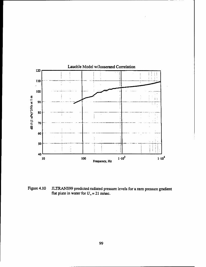
Lauchle Model w/Josserand Correlation
10 100 1 10' Frequency, Hz
110"
Figure 4.10 JLTRANS99 predicted radiated pressure levels for a zero pressure gradient flat plate in water for C/. = 21 m/sec.
99
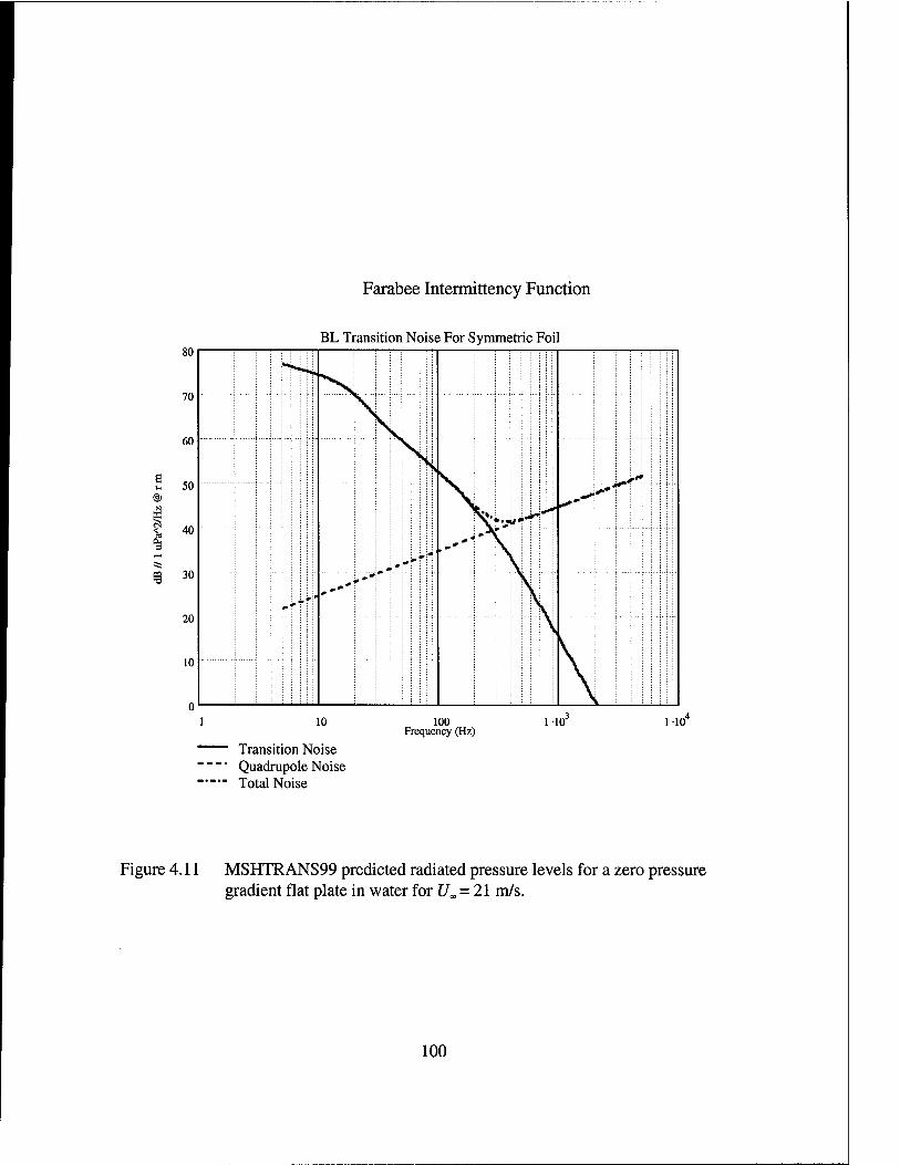
E
®
Farabee Intermittency Function
BL Transition Noise For Symmetric Foil
100 Frequency (Hz)
MO MO
Transition Noise Quadrupole Noise Total Noise
Figure 4.11 MSHTRANS99 predicted radiated pressure levels for a zero pressure gradient flat plate in water for t/OT= 21 m/s.
100
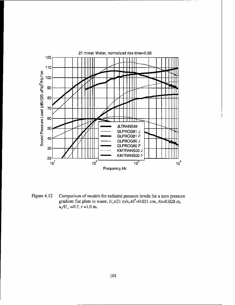
21 m/sec Water, normalized rise time=0.20
Frequency, Hz
Figure 4.12 Comparison of models for radiated pressure levels for a zero pressure gradient flat plate in water, U=21 m/s^5*=0.021 cm, zlx=0.028 m, u/U^, =0.7, r =1.0 m.
101
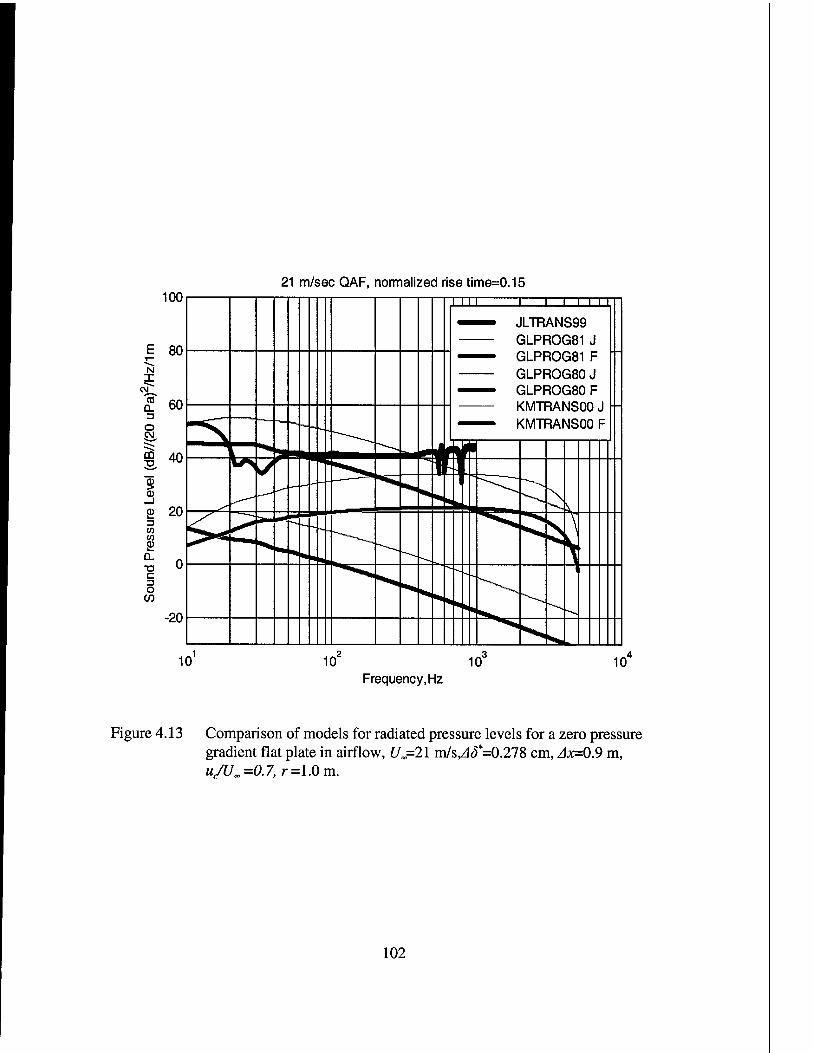
100
E 80 N X
cö Q_
O P4.
21 m/sec QAF, normalized rise time=0.15
60
40 m
9 03
£ 20 W
■o c o
-20
10'
I MI i i i 1111
—— JLTP.ANS99 V
■^— ( aLrnvmoi u 3LPROG81 F ""
vai_r nuuuu \j — GLPROG80 F
K.M I HANbUÜ J '" ^— KMTRANS00 F
4t\ f \l I I ^^^T;
10 10° 1(T Frequency, Hz
Figure 4.13 Comparison of models for radiated pressure levels for a zero pressure gradient flat plate in airflow, U<=21 m/s,J<f=0.278 cm, zlx=0.9 m, ußJm =0.7, r =1.0 m.
102
CHAPTER 5
EXPERIMENTAL APPARATUS
A significant effort was made during the ONR initiative phase of this investigation to
develop a facility with sufficiently low background noise which maintained laminar flow
over at least the first third of a test plate. The components of the entire experimental
apparatus and environment include the ARL flow-through anechoic chamber, the quiet
flow source, the flow management section, nozzle, diffuser, and the various test plates
that have been created. Further information on the facility and original planned research
use can be found in Marboe, et al. (1991). Subsequent development of a test section
located on the floor of the anechoic chamber by Brungart (1997) utilizing most of the
Quiet Airflow Facility components appeared to be much closer to the required
background noise levels to conduct the desired measurements. This facility was further
enhanced to finally create a quiet enough environment for the measurements. While not
all of the Marboe, et al. (1991) apparatus was used in the present measurements, it is
relevant to discuss the effort that went into trying to develop a facility quiet enough to
make validation measurements. This is described in more detail in Appendix B. The
difficulties encountered do emphasis perhaps how insignificant zero pressure gradient
boundary layer transition noise is when compared to other potential noise sources.
103

5.1 Quiet Airflow Facility
This facility is basically a quieted air source connected to a flow management
nozzle. The nozzle can form an open jet or a closed entrance into a test section. Several
different nozzles exist. One has a semi-circular (15.2 cm radius) orifice situated normal
to a planar baffle. A second nozzle has a square orifice 18 inches on a side. The current
nozzle has a 15.2 cm x 30.5 cm rectangular orifice. The entire Quiet Airflow Facility as
finally configured for this investigation is shown in Figure 5.1.
5.1.1 Flow-Through Anechoic Chamber
A low-frequency acoustic test facility to study the acoustics of air flow and air-
moving machinery was constructed in 1986. The ARL Penn State Flow-Through
Anechoic Chamber was designed to have a minimum cut-off frequency of 70 Hz (per ISO
standard), using fiberglass wedges. To handle the air flow requirements of an
experimental Axial Flow Research Fan, the air inlet wall provides 100 square feet of open
area to insure quiet flow. The openings are uniformly distributed over the entire wall
opposite the test facility location with openings omitted in the wedge blocks adjacent to
the side walls (Figure 5.2). Two layers of screen and perforated sheet metal help to insure
uniform distribution of flow with minimum turbulence. The exit angle between the
wedges on the air inlet wall was designed for non-turbulent flow. This final wall design
was established following a scale model study by Quartararo and Lauchle (1985).
The test facility opening to the upper control room is placed symmetrically in the
chamber so that flow distortion is at a minimum. Air can either be discharged into the
104
control room or anechoic chamber with flow return via the ceiling plenum. The floor
wedges are removable to gain access to the interior of the test volume which also allows
the facility to be used as a hemi-anechoic chamber. A modular wire mesh platform is
available for mounting experiments within the volume.
The performance characteristics of the chamber were reported in Prout and
Marboe (1990). The chamber meets the requirements of both ISO 3745 and EC 268
(International Standards 1972,1977) from 90 Hz to 12.5 kHz. Sound pressure
measurements may be made to ISO tolerances within 1.0 to 4.0 meters of the source at
frequencies as low as 70 Hz. Figure 5.3 shows sound level meter levels plotted on a set
of NCB Balanced Noise Criterion curves (Beranek, 1988). (These are revised from the
PNC curves used prior to 1988). The empty shell noise levels were approximately NCB-
26. The octave band background noise levels in the anechoic chamber meet a balanced
noise criterion of NCB-13 at the highest octave band measured (8000 Hz) and is lower
than NCB-10 in frequency bands below that. Accordingly, the chamber would have a
rating of NCB-13. An NCB-15 level had been predicted for the chamber when the wedge
system had been installed. The A-weighted overall level of the ambient noise inside the
chamber is 17 dB.
5.1.2 Air Source
A 20 HP centrifugal blower is acoustically and mechanically isolated from the
wall jet apparatus by placing it in a sound and vibration isolation box (Figures 5.4 and
5.5) that is located in the control room adjacent to the chamber. The inlet to the blower is
105
muffled and the outlet air passes through a treated labyrinth and flexible hose to the
settling chamber of the wall jet facility where turbulence management screens are located.
It was necessary to design some additional sound absorption into the plenum side of the
sound isolation box to minimize the noise traveling down the flex hose. A set of baffles
was designed to create four 90 degree turns for the flow so that higher frequency noise
would be attenuated by the Soundcoat ® 2.5 cm thick foam-lead-foam material which
was used to line the box and the baffles as shown in Figure 5.6. This treatment plus the
intake muffler significantly reduces the airborne noise from the blower.
A Buffalo Forge centrifugal blower, size 4 with wheel diameter of 42 cm, is used
as the prime air mover (Figure 5.7). It is powered by a 20 HP AC motor driven by an
ABB inverter. The motor is water cooled to decrease the build up of heat inside the foam
lined box. Pillow block bearings reduce the transmission of motor induced vibrations to
the impeller. A rubber bellows attaches the blower discharge to the attenuation plenum.
A Conic-Flow Silencer muffler has been attached to the inlet to the blower (Figure 5.5).
A capability for suction for flow management in the test section is provided by the blower
intaking air from a 10 cm hose attached to the duct between the muffler and the rubber
isolation hose into the blower. A throttle can be mounted on the muffler intake to provide
the coarse adjustment of the suction strength. However, neither the suction nor the
throttle capabilities were used either during the measurements for this investigation.
The air is discharged from the source plenum vertically through a 40 cm diameter
flexible vinyl hose and turned with a 120 degree damped sheet-metal elbow. A section of
sheet-metal 40 cm diameter tubing passed through the portal into the anechoic chamber
106

(Figure 5.8) before being turned by another elbow itself into another Conic-Flow
Silencer muffler. A piece of flexible hose attached the silencer outlet to a diffuser section
for entry in the acoustic settling plenum (Figure 5.9). The diffuser is lined with 2.5 cm
thick Soundcoat. The plenum is lined with foam acoustic wedges. The wedges are
Illbruck SONEXsuper ™ 15.24 cm high foam with 3 wedges in a 30.5 cm by 30.5 cm
square. Their sound absorption characteristics are listed in Table 5.1. A square bell
mouth was constructed out of split, 8 cm PVC pipe. This provides a smooth inlet into
the flow management section.
Table 5.1 Sound Absorption Coefficients of Foam and Wedges Used in QAF
Frequency (Hz) SONEXsuper Wedges Soundfoam Embossed
125 0.18 0.15
250 0.86 0.45
500 1.22 0.70
1000 1.24 0.92
2000 1.14 0.97
4000 1.20 0.98
5.1.3 Flow Management
The preceding plenum, diffuser, and settling chamber with flow management
screens are shown in Figure 5.10. Ten layers of screens are used to reduce turbulence and
create as homogeneous a flow as possible. The entire assembly is mounted on rubber
pads for vibration isolation. Care was taken to make all corners within the settling
chamber and nozzle as smooth as possible to help maintain laminar irrotational flow.
107
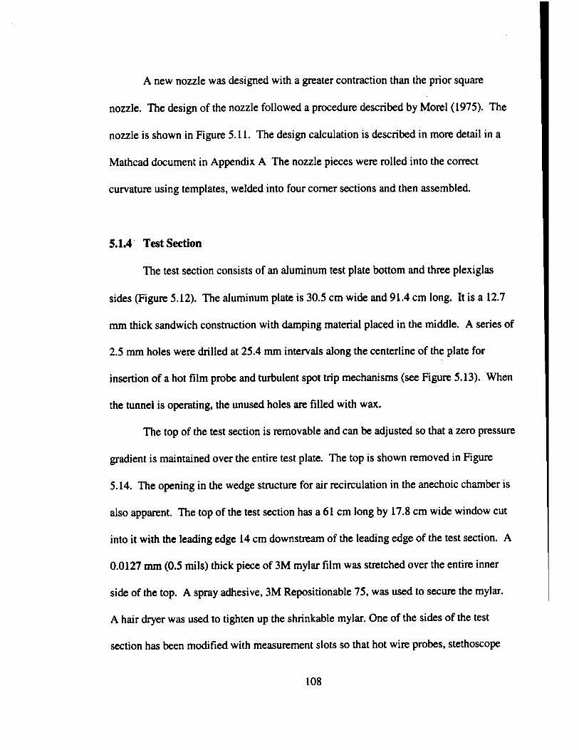
A new nozzle was designed with a greater contraction than the prior square
nozzle. The design of the nozzle followed a procedure described by Morel (1975). The
nozzle is shown in Figure 5.11. The design calculation is described in more detail in a
Mathcad document in Appendix A The nozzle pieces were rolled into the correct
curvature using templates, welded into four corner sections and then assembled.
5.1.4 Test Section
The test section consists of an aluminum test plate bottom and three plexiglas
sides (Figure 5.12). The aluminum plate is 30.5 cm wide and 91.4 cm long. It is a 12.7
mm thick sandwich construction with damping material placed in the middle. A series of
2.5 mm holes were drilled at 25.4 mm intervals along the centerline of the plate for
insertion of a hot film probe and turbulent spot trip mechanisms (see Figure 5.13). When
the tunnel is operating, the unused holes are filled with wax.
The top of the test section is removable and can be adjusted so that a zero pressure
gradient is maintained over the entire test plate. The top is shown removed in Figure
5.14. The opening in the wedge structure for air recirculation in the anechoic chamber is
also apparent. The top of the test section has a 61 cm long by 17.8 cm wide window cut
into it with the leading edge 14 cm downstream of the leading edge of the test section. A
0.0127 mm (0.5 mils) thick piece of 3M mylar film was stretched over the entire inner
side of the top. A spray adhesive, 3M Repositionable 75, was used to secure the mylar.
A hair dryer was used to tighten up the shrinkable mylar. One of the sides of the test
section has been modified with measurement slots so that hot wire probes, stethoscope
108
burst probes, and anemometer probes could be inserted. The forward slots were
eventually replaced with a 20.3 cm long by 10.2 high window cut into it with the leading
edge 5.1 cm downstream of the leading edge of the test section. It was covered in mylar
in a manner similar to above. A downstream slot was located at 85.75 cm downstream of
the leading edge of the test section. Typically, the inside of the slot would be covered
with clear tape and a small hole would be made to accommodate the desired probe.
By surveying over the plate with a capillary total head tube on a stethoscope
(Figure 5.15), the bursting typical of transition was found to occur near the trailing edge
of the test and working forward as velocity was increased. Side wall turbulent
contamination is generally thought to expand at an angle of about 10 degrees from the
corner juncture of the walls of the test section (Motohashi and Blackwelder, 1983). This
contamination should join across the test section nearly at the end of the test section.
5.1.5 Half-Plane
A half-plane is also available for the test section. The splitter plate is 1.75 cm
thick. A nose portion (aluminum) is the leading 12.4 cm of the plate. It is attached to
another 71.3 cm long plate (aluminum anodized blue) as shown in Figure 5.16. The
leading edge follows design guidance from Narasimha and Prasad (1995) using a nose
length of 3 times the plate thickness. The super-elliptic profile is given by:
a-x a
n = 1 , 0<,x<.a n>2 (5.1)
where
109
a length of the nose
b half-thickness of the plate
n was 2.5 for this application.
A diffuser insert can be attached to the trailing edge of the plate for a smooth transition to
diffusion.
5.1.6 Diffuser
A new diffuser needed to be designed to work with the rectangular test section.
The trick in diffuser design is to diffuse the flow, slowing it down, as quickly as possible
without creating flow separation on the diffuser walls. This was especially necessary in
the configuration being used in this investigation because of the limited distance from the
test section to the wall of the anechoic chamber. As it was, the discharge was purposely
pointed toward the air outlet wall and the anechoic wedges were removed in that area.
Soundcoat material was placed along the wall of the chamber at a slight angle to reduce
direct refection back into the diffuser.
The diffuser was designed following a method described by Kline, Abbott, and
Fox (1959). Details can be found in section B.5. Even though the design methodology
was followed, the diffuser walls were still prone to a transitory stall bubble that resulted
in unsteady flow discharging from the diffuser. The final configuration created an
operating point just on the edge of another stall avoidance criterion later found in Barlow
et al. (1999). However, that unsteadiness did not propagate back upstream into the test
section based on the hot wire measurements near the trailing edge of the test section.
110
The diffuser was lined with 2.5 cm thick embossed Soundcoat ® to absorb sound
propagating down the diffuser and any reflections back from downstream. The lining is
shown in Figure 5.17. The absorption properties of the material are included in Table 5.1.
With the mylar window in the top of the test section, it was necessary to increase
the resistance at the end of the diffuser to increase the pressure in the test section so the
mylar was not drawn down into the test section. This draw down introduced significant
asymmetry in the flow when it first occurred. The test requires that the flow on the top
and bottom of the test section be the same so the intermittency measurements could be
made along with the acoustic measurements. Four 1.2 cm thick fibrous filters were used
to provide this resistance. These are also shown in Figure 5.17. This had the added
advantage of eliminating any transitory stall in the diffuser.
5.2 Instrumentation and Signal Processing
5.2.1 Hot Wire Anemometry
5.2.1.1 Probe Positioning
Measurement probes are positioned in the test section with a three dimensional
Velmex traversing mechanism, accurate to 25.4 jim, through two, 6.35 mm wide slots cut
in the plexiglass tunnel sidewall. A Mitutoyo digital caliper, also accurate to 25.4 /im,
attached to the vertical stage of the mechanism to facilitate the measurement of boundary
layer velocity profiles. Additionally, the vertical stage is equipped with a rotation stage,
thereby allowing a measurement probe to be rotated relative to the test section axis for
added ease of probe positioning. The Velmex traversing mechanism is attached to a
111
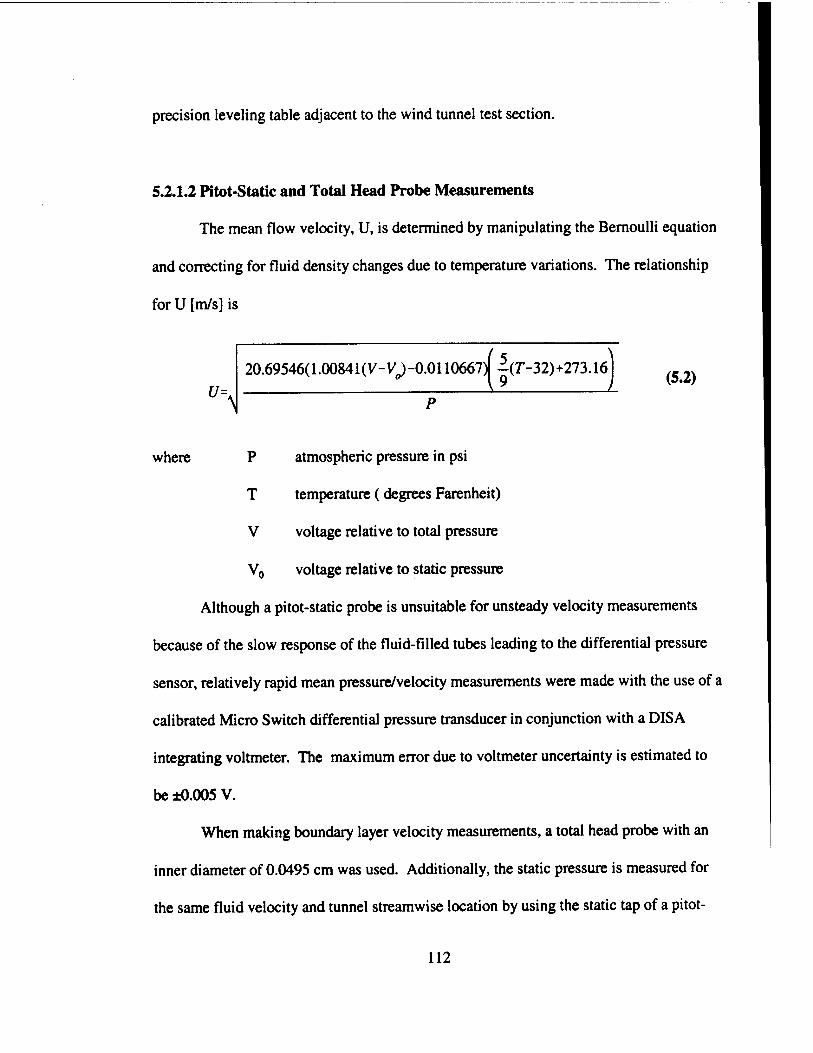
precision leveling table adjacent to the wind tunnel test section.
5.2.1.2 Pitot-Static and Total Head Probe Measurements
The mean flow velocity, U, is determined by manipulating the Bernoulli equation
and correcting for fluid density changes due to temperature variations. The relationship
for U [m/s] is
(5.2)
where P atmospheric pressure in psi
T temperature (degrees Farenheit)
V voltage relative to total pressure
V0 voltage relative to static pressure
Although a pitot-static probe is unsuitable for unsteady velocity measurements
because of the slow response of the fluid-filled tubes leading to the differential pressure
sensor, relatively rapid mean pressure/velocity measurements were made with the use of a
calibrated Micro Switch differential pressure transducer in conjunction with a DISA
integrating voltmeter. The maximum error due to voltmeter uncertainty is estimated to
be ±0.005 V.
When making boundary layer velocity measurements, a total head probe with an
inner diameter of 0.0495 cm was used. Additionally, the static pressure is measured for
the same fluid velocity and tunnel streamwise location by using the static tap of a pitot-
112
static probe. Pitot-Static probes may be used for velocity measurements only when at
least five probe diameters separate the wall and the probe. This avoids the creation of a
venturi passage between the wall and the probe. Otherwise, the flow would be
accelerated, thereby lowering the static pressure on one side of the probe, resulting in
inaccuracies in static pressure; consequently, imprecise fluid velocities would be
obtained. When conditions permitted, a 0.132 cm diameter pitot-static probe was used.
5.2.13 Hot Wire Anemometer Measurements
Both mean and fluctuating velocities were measured with a two channel TSIIFA
300 Research Constant Temperature Anemometer. The anemometer is controlled with
TSI's ThermalPro software via an RS232 interface with a Gateway 2000 486 DX2 66V
personal computer. A high speed A/D converter, mounted internal to the computer, is
used to convert the analog data output from the anemometer to digital data for
manipulation. Hot-wire data are sampled at a frequency of 10 kHz with a low pass filter
set at 5 kHz. Data are acquired for a period of 6.5536 seconds resulting in 64,000 points
at each measurement location. Typically, an overheat ratio (the ratio of operating
resistance to actual hot wire resistance) of 1.72 was used. The ThermalPro software
calculates the velocity statistics up to the fourth order moment (i.e., kurtosis). All data
are archived on Zip disks using an Iomega Zip 100 drive connected to the host computer.
The hot-wire probes are visually aligned in the flow field and positioned as
required with the Velmex traversing mechanism. A TSI Model 1218E Boundary Layer
Probe constructed of a single 5 fim diameter platinum-coated tungsten wire with a
113
sensing area length of 1.27 mm was used for streamwise velocity measurements.
Single component wires are calibrated in-situ over a range of velocities from 0.0
m/s to 25.0 m/s with pi tot-static probe measurements as the known standard. TSI's
ThermalPro software generates a calibration curve for every probe calibration and
calculates the mean square error which is usually less than 0.3. Probe velocity
calibrations are checked prior to every profile measurement to minimize errors. The
experiment temperature is checked throughout each data run so as to correct for
deviations from the calibration temperature. Equations (5.3) and (5.4) illustrate how a
small change in temperature can cause an erroneous fluid velocity to be determined if the
temperature departure is not appropriately accounted for.
*=**. (5.3)
where E,, wheatstone bridge voltage
T, hot-wire sensor operating temperature
Tc hot-wire sensor calibration temperature
Te hot-wire sensor experiment temperature
Veff = K+AE+BE2+CE3+DE4 (5.4)
where V^ = effective velocity (velocity component normal to the hot-wire)
K, A, B, C, and D are calibration constants
For example, if the experiment temperature where to unaccountably increase, the
114
effective velocity as determined from Equation (5.4) would be lower than the actual
velocity.
Because hot-wire probes are calibrated against pitot-static probes and due to the
sensitivity of hot-wire measurements to temperature changes, pitot-static probe mean
velocity measurements are considered more accurate than hot-wire measurements.
5.2.1.4 Handheld Anemometry
Velocity measurements were also made in the test section with a TSI Model
8345 VelociCalc handheld anemometer (S/N 00030146). It has an accuracy of 3% of
scale (or ±0.015 m/sec, whichever is greater) although the calibration was less than
1.7%. This anemometer reads from 0 to 30 m/sec with a resolution of 0.01 m/sec. It was
used to verify flow conditions and temperature in the test section.
5.2.2 Sound Pressure
The single channel sound pressure measurements used for diagnostics are made
with a Brilel & Kjaer Type 4135 V2 inch microphone (serial number 1946536) with Type
2670 preamplifier (serial number 2003873). A Briiel & Kjaer Type 5935L power supply
and amplifier (serial number 2016632) is used with linear weighting set. The amplifier is
capable of -5 to +55 dB gain. It is battery powered for low noise. If necessary, a Krohn-
Hite 3342 2 channel filter (serial number 216) is used as a high pass filter to remove very
low frequency facility noise. This is then input to the DSP Technologies SigLab signal
analyzer described in section 5.2.5. The procedures for use of the acoustic intensity
115
methods are well documented in Fahy (1989).
5.23 Acoustic Intensity
The two channel sound intensity measurements are made with a Bruel & Kjaer
Type 4178 Intensity Vi inch microphone set consisting of Type 4135 microphone (serial
number 1946506) with Type 2670 preamplifier (serial number 2003871) for channel 1
and Type 4135 microphone (serial number 1946464) with Type 2670 preamplifier (serial
number 2003873) for channel 2. Otherwise, the signal processing equipment is the same.
Table 5.2 provides a full list of equipment used for the time-averaged intensity method.
The microphones are generally placed outside of the mylar windows. The
acoustic transparency of this material was established by Kargus and Lauchle (1997).
The insertion loss is generally less than 3 dB with deviations less than 1 dB from 300 Hz
to 3 KHz.
5.23.1 Real-Time Analog Intensity Circuitry
A real-time active acoustic intensity circuit has been developed to provide a signal
that can be processed along with a hot film shear stress sensor to yield a coherent output
intensity similar to coherent output power processing. Figure 5.19 provides a process
diagram.
The electronic circuit was designed and fabricated by Todd Batzel of ARL Penn
State. It is described in detail in Appendix C including circuit diagrams. The gains in the
circuitry are multiply by 250 at the input filter, multiply by 295 in the integrator,
116
and divide by 10 in the multiplier. This gives a total gain multiplier of 7375
or 38.7 dB. A high pass filter has been implemented with a cut-off at 30 Hz. The filter is
a fourth order Bessel filter with linear phase. This was chosen for this particular
application in order to remove some low frequency tunnel noise that otherwise would
have used up about 40 dB of dynamic range. A reset button is installed for the integrator
to allow re-zeroing in case of a built up bias. The circuit can be powered by two onboard
9V batteries or an AC adapter.
5.2.3.2 Calibration
Two plane wave tubes were fabricated for calibration of the two microphone intensity
probe. They cover frequency ranges 800-5270 Hz and 70-950 Hz, respectively. They are PVC
pipe with aluminum ends for probe mounting. They are shown in Figure 5.18. Further
details are provided in Table 5.3. The individual microphones are also calibrated with a
Brüel & Kjaer Type 4220 pistonphone (serial number 347321).
117
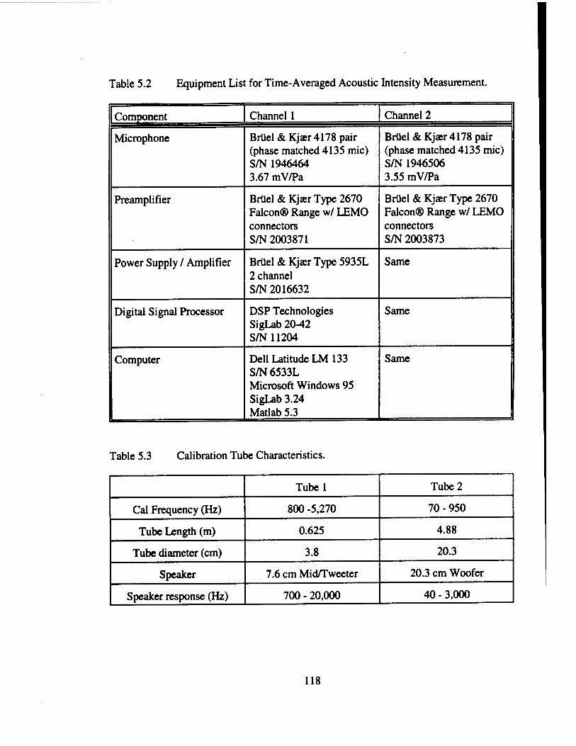
Table 5.2 Equipment List for Time-Averaged Acoustic Intensity Measurement.
Component Channel 1 Channel 2
Microphone Briiel&Kja* 4178 pair (phase matched 4135 mic) S/N1946464 3.67 mV/Pa
Brüel «ScKjaer 4178 pair (phase matched 4135 mic) S/N1946506 3.55 mV/Pa
Preamplifier Brüel & KjaerType 2670 Falcon® Range w/ LEMO connectors S/N2003871
Brüel & Kjaer Type 2670 Falcon® Range w/ LEMO connectors S/N 2003873
Power Supply / Amplifier Brüel & KjaerType 5935L 2 channel S/N 2016632
Same
Digital Signal Processor DSP Technologies SigLab 20-42 S/N11204
Same
Computer Dell Latitude LM 133 S/N 6533L Microsoft Windows 95 SigLab 3.24 Matlab 5.3
Same
Table 5.3 Calibration Tube Characteristics.
Tubel Tube 2
Cal Frequency (Hz) 800 -5,270 70 - 950
Tube Length (m) 0.625 4.88
Tube diameter (cm) 3.8 20.3
Speaker 7.6 cm Mid/Tweeter 20.3 cm Woofer
Speaker response (Hz) 700 - 20,000 40-3,000
118
5.2.4 Coherent Output Intensity
The signal processing diagram for the calculation of coherent ouput intensity is
provided in Figure 5.18. The output of the real-time active intensity processing circuit is
input to channel 1 of the SigLab analyzer. The output of the TSI anemometer is input to
channel 2 of the SigLab analyzer. The coherence is computed and multiplied along with
microphone sensitivity and other constants with channel 1 to yield the desired coherent
output intensity. This is all covered in more detail in Appendix C.
5.2.4.1 Hot Film Sensor
The hot film signals are measured with a TSI Incorporated model 1750 constant
temperature anemometer (serial number 2318). A TSI probe model 1237-10 (serial
number 984071) is inserted flush into holes in the test plate. A 31 ohm control resistor is
necessary. The holes were spaced 25.4 mm apart longitudinally along the centerline of
the test plate. The other holes were waxed over.
5.2.4.2 Conditioning with a Shear Stress Sensor
It is desired to apply the power of coherent output processing to the acoustic
measurements. In this case, it is assumed that shear stress due to passage of a turbulent
spot is caused by the same physical phenomenon (i.e. growth of the spot) that results in
acoustic radiation. Therefore, there should be coherence between those signals. The
noise associated with each sensor is assumed to be independent. Hot films have been
shown to be insensitive to acoustic noise. The coherence is calculated using Equation
119
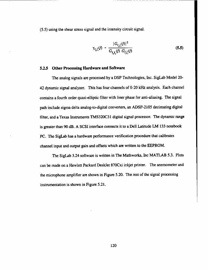
(5.5) using the shear stress signal and the intensity circuit signal.
'o'o 'rr
5.2.5 Other Processing Hardware and Software
The analog signals are processed by a DSP Technologies, Inc. SigLab Model 20-
42 dynamic signal analyzer. This has four channels of 0-20 kHz analysis. Each channel
contains a fourth order quasi-elliptic filter with liner phase for anti-aliasing. The signal
path include sigma delta analog-to-digital converters, an ADSP-2105 decimating digital
filter, and a Texas Instruments TMS320C31 digital signal processor. The dynamic range
is greater than 90 dB. A SCSI interface connects it to a Dell Latitude LM 133 notebook
PC. The SigLab has a hardware performance verification procedure that calibrates
channel input and output gain and offsets which are written to the EEPROM.
The SigLab 3.24 software is written in The Mathworks, Inc MATLAB 5.3. Plots
can be made on a Hewlett Packard DeskJet 870Cxi inkjet printer. The anemometer and
the microphone amplifier are shown in Figure 5.20. The rest of the signal processing
instrumentation is shown in Figure 5.21.
120
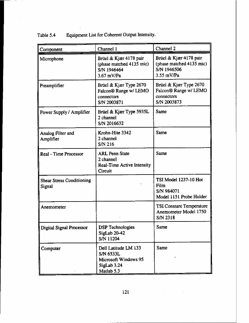
Table 5.4 Equipment List for Coherent Output Intensity.
| Component Channel 1 Channel 2
Microphone Briiel&Kjaer 4178 pair (phase matched 4135 mic) S/N1946464 3.67 mV/Pa
Briiel & Kjaer 4178 pair (phase matched 4135 mic) S/N1946506 3.55 mV/Pa
Preamplifier Briiel&Kjaer Type 2670 Falcon® Range w/ LEMO connectors S/N 2003871
Briiel&Kjaer Type 2670 Falcon® Range w/ LEMO connectors S/N 2003873
Power Supply / Amplifier Briiel & Kjaer Type 5935L 2 channel S/N 2016632
Same
Analog Filter and Amplifier
Krohn-Hite 3342 2 channel S/N 216
Same
Real - Time Processor ARL Penn State 2 channel Real-Time Active Intensity Circuit
Same
Shear Stress Conditioning Signal
■
TSI Model 1237-10 Hot Film S/N984071 Model 1151 Probe Holder
Anemometer TSI Constant Temperature Anemometer Model 1750 S/N2318
Digital Signal Processor DSP Technologies SigLab 20-42 S/N 11204
Same
Computer Dell Latitude LM 133 S/N 6533L Microsoft Windows 95 SigLab 3.24 Matlab 5.3
Same
121
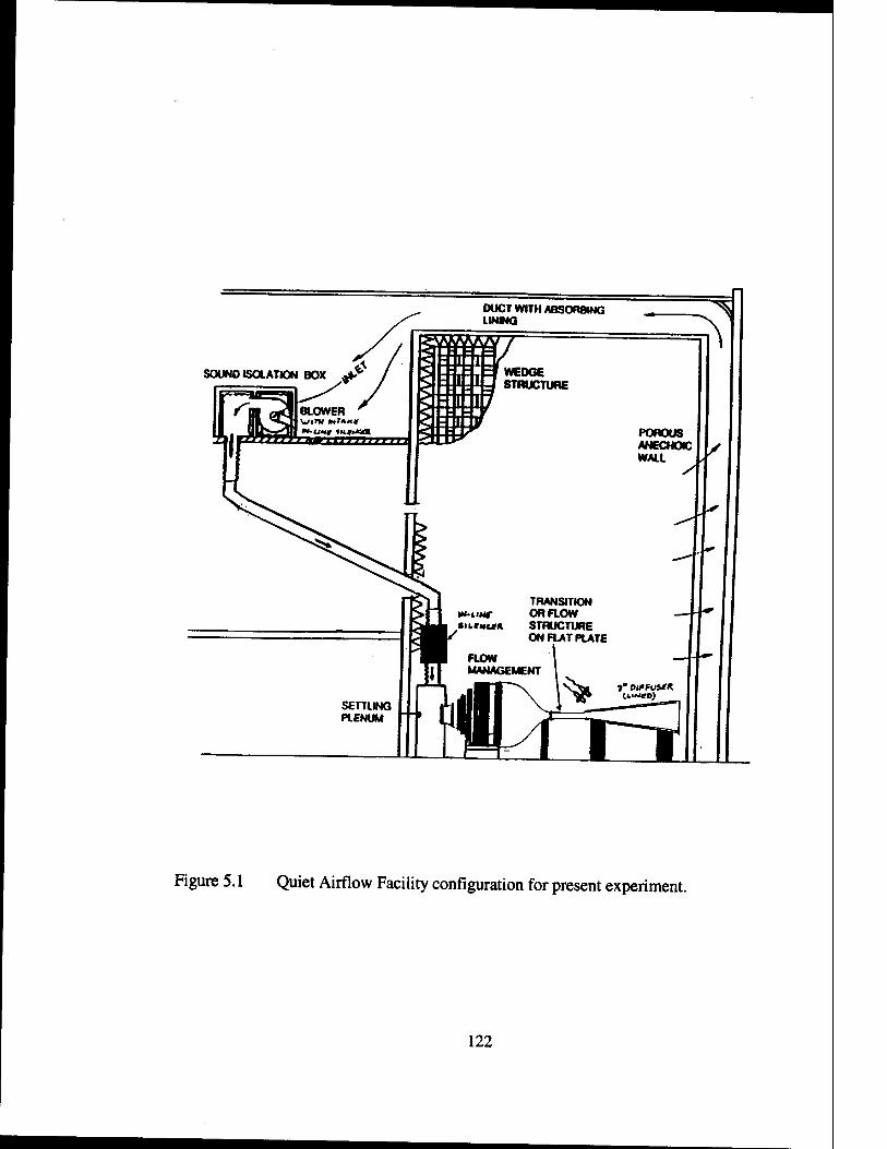
Figure 5.1 Quiet Airflow Facility configuration for present experiment.
122

AIR RETURN PLENUM
FACILITY MOUNTING ACCESS
TURNING VANE
PLENUM
AIR INLETS
CUT-OFF FREQUENCY 70 Hz
WEDGE STRUCTURE Il.1mhx7.3mw x 8.8md
WORKING VOLUME 9.3 m h x 5.5 m w x 6.8 m d
Figure 5.2 Flow-through anechoic chamber.
123
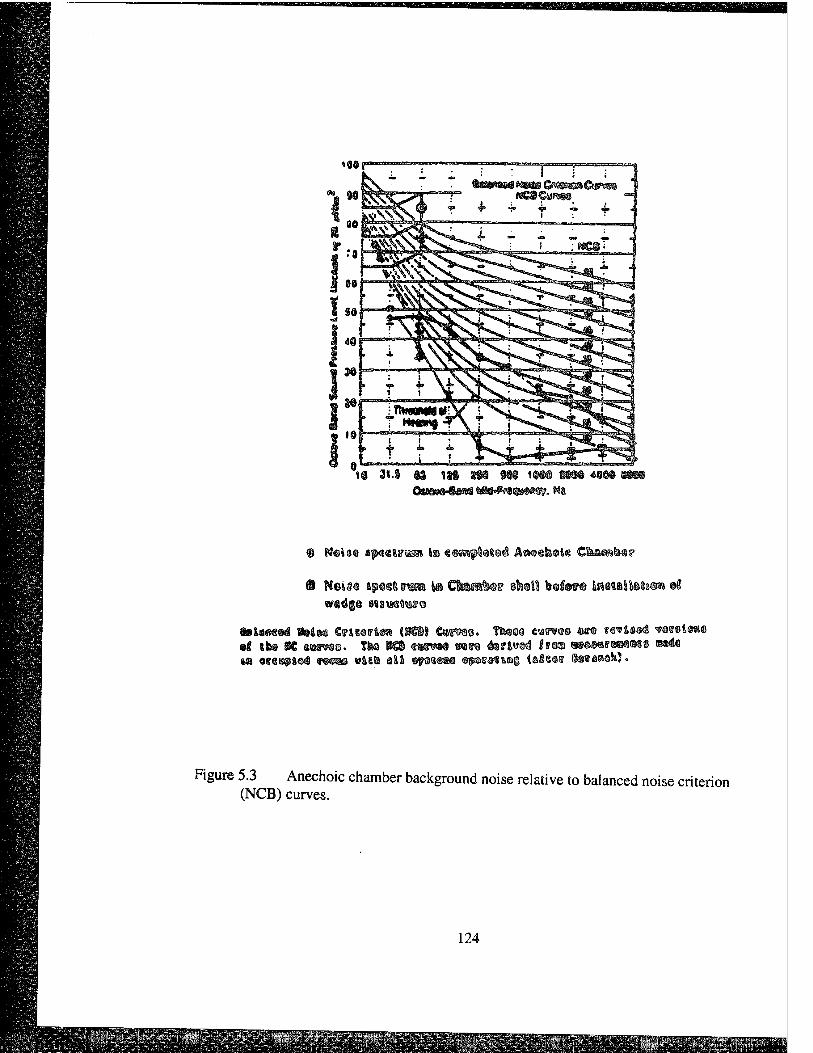
Ǥe
ti ii.i m it§ m m® *m MB
® fffels« «p*«tr«rai to «««npt«ted A««ehete Ctemi@?
© N»in ipctnm to ©terni» ski« fe«I©w i&staltotB®» «C
§8ltM«H§ Mtü CrtMriM (MM CUTM«. TMM WWM «M wit* vmitM
ass esutifM VMM «life all tf»MM ®pica<s&ii§ <A<«09 ©SMINM.
Figure 5.3 Anechoic chamber background noise relative to balanced noise criterion (NCB) curves.
124
mm SS^K BBEansfioagraH
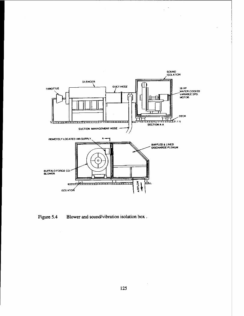
THROTTLE
SILENCER
rT-n-T-mfr
DUCT HOSE
L u
111111111111111111111111 ii 111111
SUCTION MANAGEMENT HOSE
JL
SOUND ISOLATION
(D
[ aaQ ii n1
20 HP WATERCOOLED
'VARIABLE SPD MOTOR
UI.LLIJ.t-1-U LJ II I J.LI.LU-Ll.i:
.DECK
-1) LILLIXlJTTTJ-rm LI LU-tl-i:i|
SECTION A A
REMOTELY LOCATED AIR SUPPLY
BUFFALO FORGE CO BLOWER
ISOLATOI
BAFFLED t LINED DISCHARGE PLENUM
Figure 5.4 Blower and sound/vibration isolation box .
125
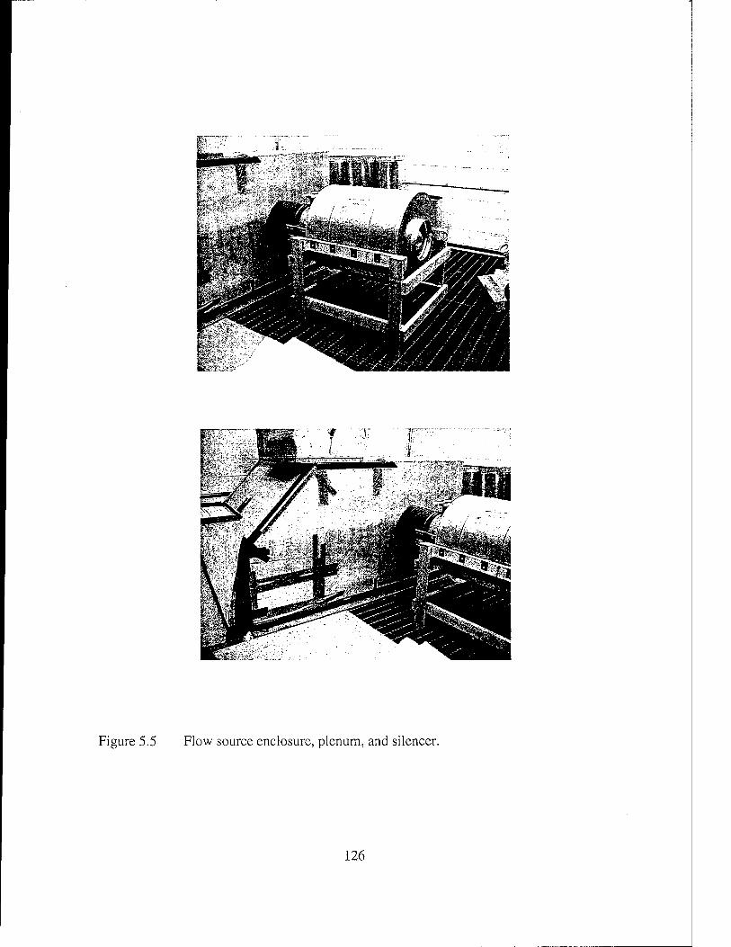
Figure 5.5 Flow source enclosure, plenum, and silencer.
126
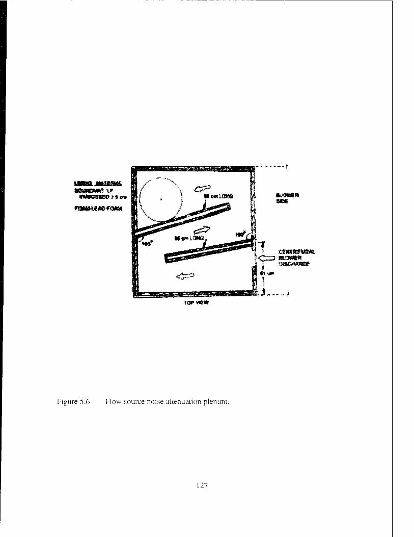
fMQCKOJttm
www
•LCMH«
ROWER fXSCWMWE
Figure 5.6 Flow source noise attenuation plenum.
127
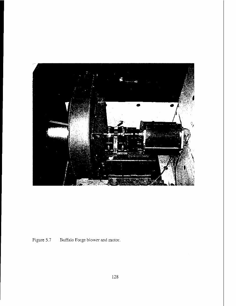
Figure 5.7 Buffalo Forge blower and motor.
128
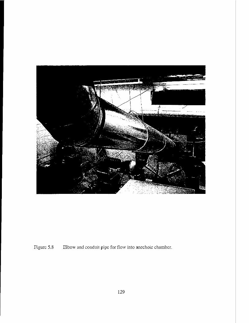
Figure 5.8 Elbow and conduit pipe for flow into anechoic chamber.
129
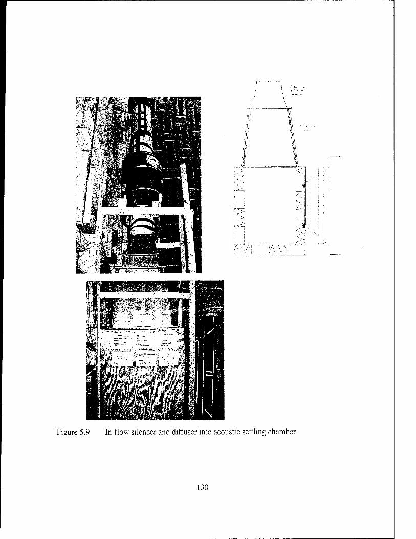
it-
i
1A A W IA:_V.1
Figure 5.9 In-flow silencer and diffuser into acoustic settling chamber.
130
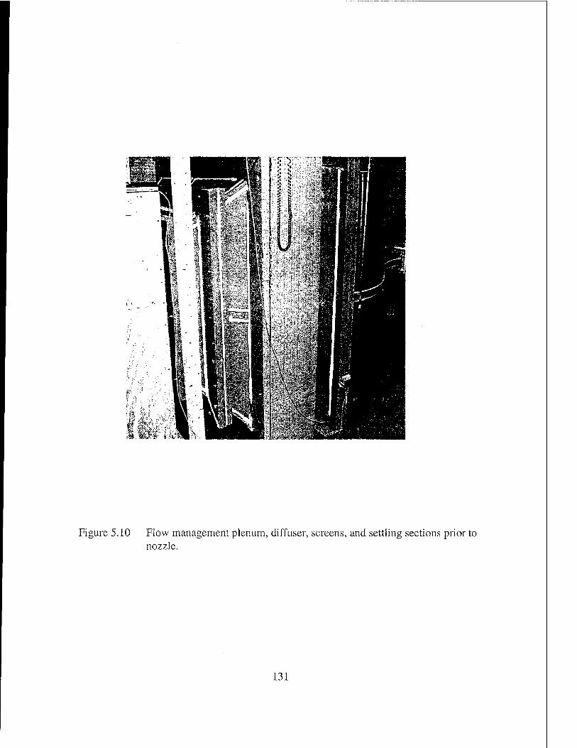
Figure 5.10 Flow management plenum, diffuser, screens, and settling sections prior to nozzle.
131
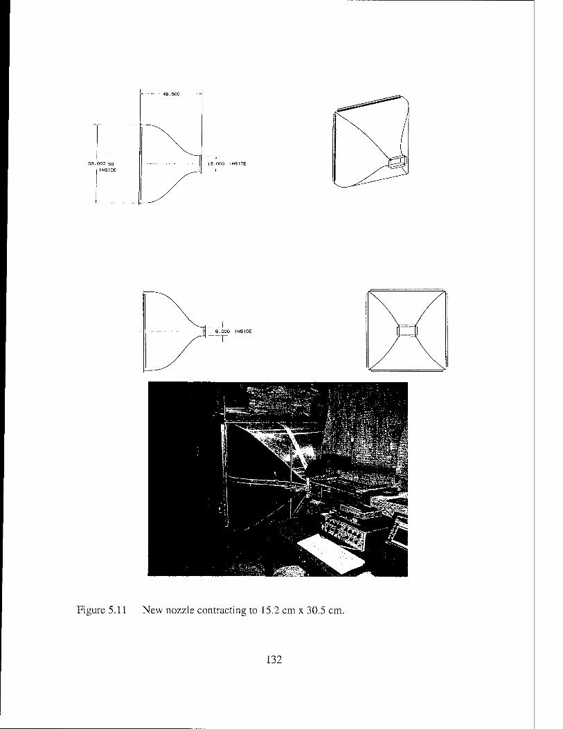
53.000 SO INSIDE
I 2.OOO 1NSIDG
Figure 5.11 New nozzle contracting to 15.2 cm x 30.5 cm.
132
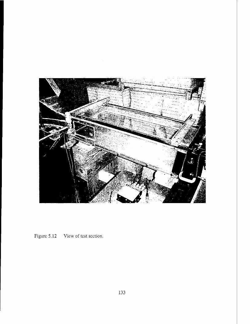
Figure 5.12 View of test section.
133
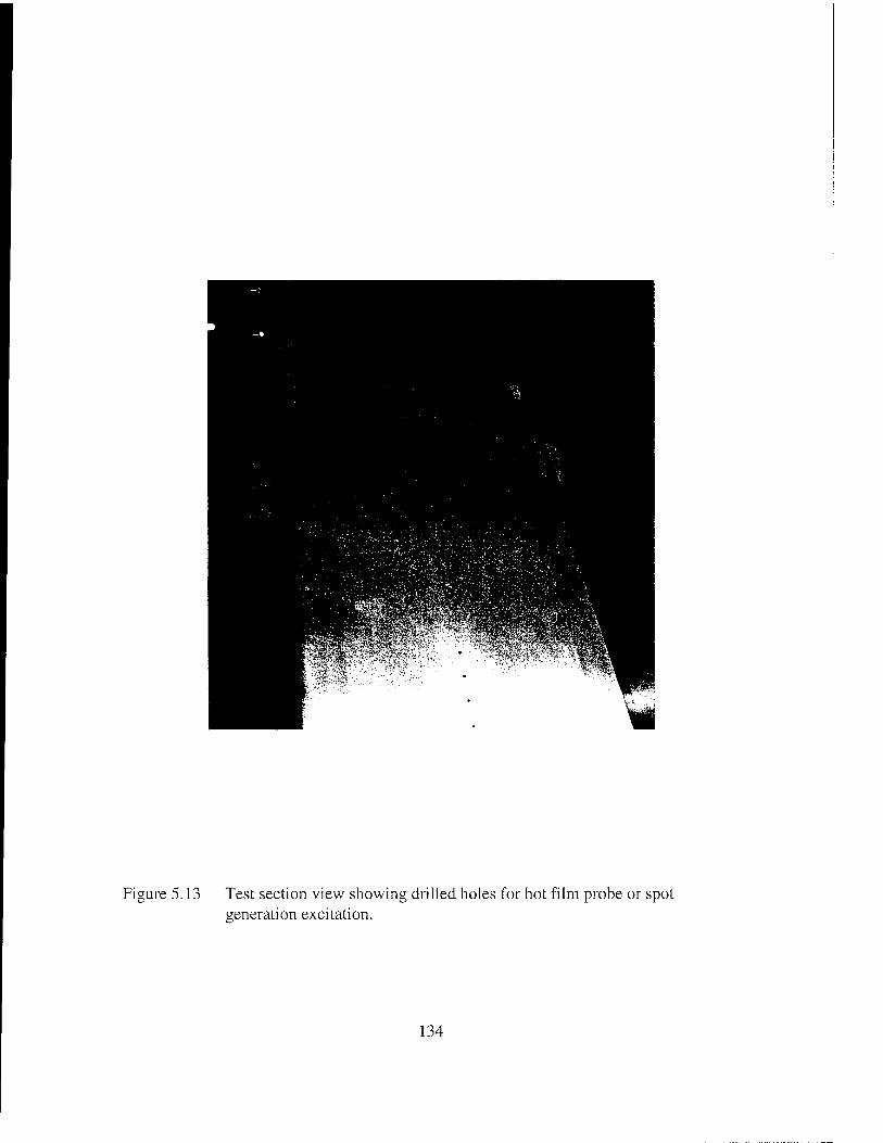
Figure 5.13 Test section view showing drilled holes for hot film probe or spot generation excitation.
134
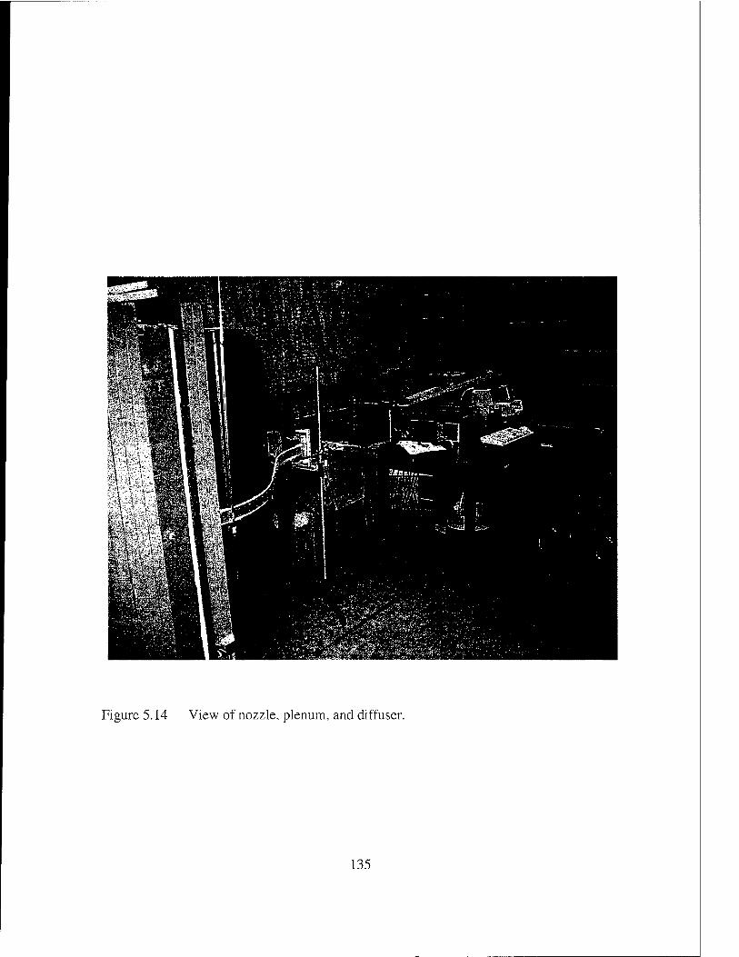
Figure 5.14 View of nozzle, plenum, and diffuser.
135

Figure 5.15 Stethoscope burst probe and tuft wand.
136
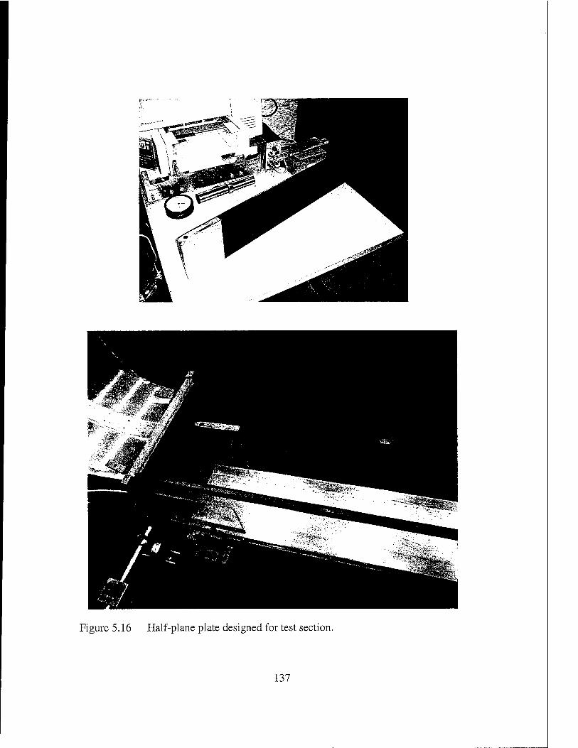
Figure 5.16 Half-plane plate designed for test section.
137
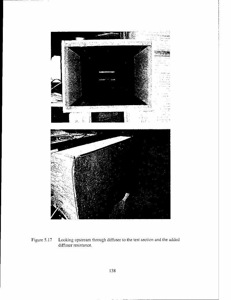
Figure 5.17 Looking upstream through diffuser to the test section and the added diffuser resistance.
138

(a)
(b)
Figure 5.18 Intensity probe calibration tubes, (a) high frequency and (b) low frequency
139
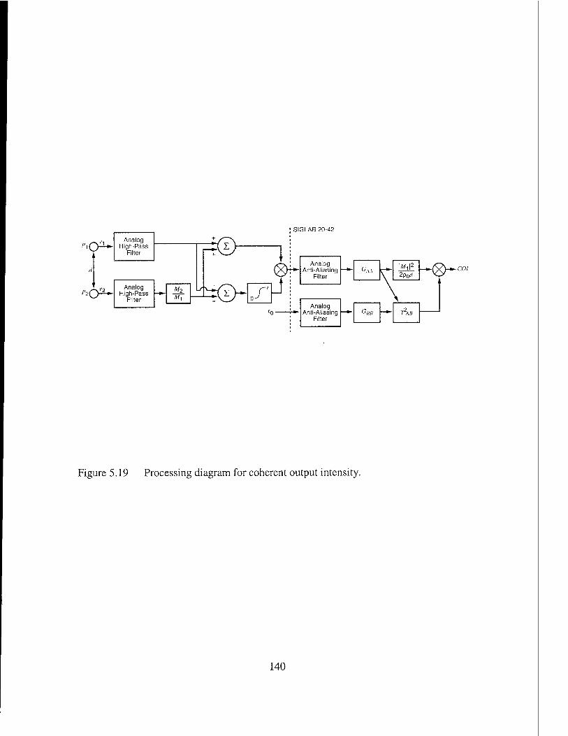
Analog High-Pass
Filter
Analog High-Pass
Filter
i&
\^y
SIGLAB 20-42
Analog Anti-Aliasing
Filter
Analog Anti-Aliasing
Filter
G,u c !-Wil2
2p0'' HS \
V ,
G«fl —^ v2.,«
-co/
Figure 5.19 Processing diagram for coherent output intensity.
140
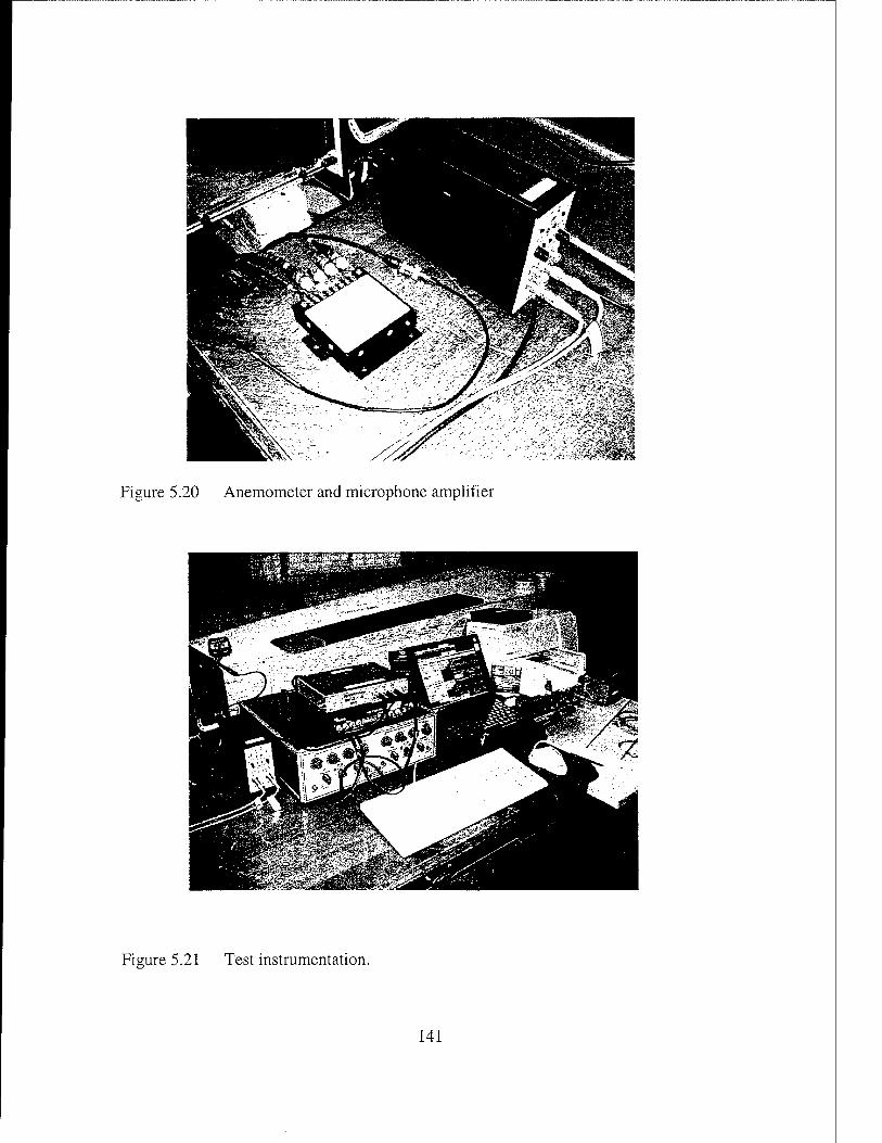
Figure 5.20 Anemometer and microphone amplifier
Figure 5.21 Test instrumentation.
141
CHAPTER 6
MEASUREMENT RESULTS
6.1 Test Section Flow
The test section flow was characterized at two longitudinal locations in the test
section using hot wire anemometry. These were x = 7.6 cm and 77.5 cm of the test
section. The forward measurement was used to establish that there was uniform laminar
entering the test section. This is shown in Figure 6.1 for two tunnel velocities and
compared to the Blasius boundary layer profile. The uniformity across the test section
area is seen in Figure 6.2. The hot wire measurements were made traversing across the
test section at heights of 25, 50, and 75% of the vertical dimension of the test section.
The variation is less than 1%. It should be noted that these measurement were conducted
prior to the addition of the resistance on the end of the diffuser which was done during
the acoustic measurements. Thus, the top velocity in the test section is higher than could
be achieved for the acoustic measurements.
The downstream measurement location was used to establish a zero pressure
gradient flow condition. Spacers were placed under the support arms on the test section
top until the proper uniformity of flow was achieved. A similar survey uniformity was
completed at this location. Those results are shown in Figure 6.3.
A 15 cm strip of 6.3 mm mesh screen placed near the leading edge of the test
section was used to trip the boundary layer in order to check the fully developed turbulent
142
flow at the end of the test section. Figure 6.4 shows a comparison of the boundary layer
profiles and turbulence intensities for this test and similar data taken with a separate
nozzle and test section in the Quiet Airflow Facility. The flow behavior appears normal
with this nozzle and test section.
6.2 Intensity Measurement Calibration
A calibration sequence was performed with the intensity instrumentation. The
configuration for a free-field calibration is shown in Figure 6.5. The SigLab signal
generator was used to provide a 2.5 Vrms, 10 kHz bandwidth white noise input to a 25
cm woofer speaker mounted in a wooden baffle. The intensity probe was positioned
above the speaker 81 cm. Reflections were minimized by use of 13 cm thick fiberglas
pads.
Before the speaker test was done, the microphones were amplitude calibrated
using the pistonphone. A magnitude and phase mismatch test was performed in the small
calibration tube (Figure 6.6). The microphones were extended into the tube to make sure
that the pressure compensation holes on the preamplifiers were exposed. This is the
reason for the notable spikes around 2 kHz. This corresponds to a quarter wavelength for
reflection from the end wall of the tube back to the microphone. The phase error is
generally less than 0.4 degrees and the magnitude error is less than 0.5 dB. For this
instrumentation phase error, the intensity error is 0 to -1 dB down to 60 Hz. The
microphones have a 25.4 mm spacing. This spacing produces an accuracy within 1.0 dB
over a range of 320 to 2500 Hz. Above this, the error increases to 5 dB at 5000 Hz.
143
There are also bias errors associated with the type of source field and the
measurement distance (Fahy, 1989). This bias error is shown for point monopole and
dipole fields, and a measurement distance of 5 cm in Figure 6.7. The effect is very small
below 3 KHz. All of the mentioned biases apply in the same manner to each of the
measurements conditions, so relative amplitude differences are still meaningful. The
random error was reduced by taking 256 averages for each measurement which yields a
±0.4 dB random error for the cross-spectrum used in the analysis.
The results of the speaker calibration verification is shown in Figure 6.8. The P-P
intensity is compared to the far field intensity determined by P^/pc. The agreement is
very good down to about 150 Hz where the near-field errors increase and produce the
amplitude fluctuations seen in the figure. Above 3.5 kHz, the discrepancy is due to finite-
difference approximations. The test section top with the mylar window was then placed
between the speaker and the intensity probe. The results in Figure 6.8b show generally
good agreement with narrowband deviations being more pronounced with the mylar.
Figure 6.9 shows the same data processed using 50 Hz constant bandwidth and 1/3 octave
bandwidths. This shows agreement within 1 dB over the frequency range of interest from
250 Hz to 3 kHz.
The value of the use of an intensity probe (with its cosine directivity) over a single
microphone is shown in Figure 6.10. A 5-12 dB improvement in signal-to-noise ratio is
achieved. The equivalent pressure level converted from the intensity level is compared to
the pressure level from only microphone 1 of the intensity probe for two measurement
locations.
144
63 Flat Plate Natural Transition Zone
Acoustic active intensity measurements were made for a natural transition zone
occurring on the top surface of the test section. The tunnel was run at its highest possible
velocity condition of 21 m/sec. In this case, the transition began just downstream of the
mylar window leading edge. The downstream edge of the mylar window was at about
65% of the transition zone. It is within this range that the predominant portion of the
radiated acoustics has been predicted to occur according to Audet et al.(1989a,b) as
shown in Figure 2.2. Any further extension of the mylar window would have been
unpractical due to a weakening of its structure and higher likelihood of surface dynamics.
A longitudinal survey was conducted over the mylar window with the probe orientation
normal to the window as shown in Figure 6.11.
Hot film measurements were made by inserting the hot film through predrilled,
but waxed over, holes in the bottom of the test section. It is presumed from the uniform
flow measured previously that the boundary layer growth and transition on the bottom of
the test section matches that on top of the test section. A comparison is made in Figure
6.12 of the locations and amplitudes of the measured intermittency to the Josserand
intermittency function.
The intermittency was determined using the circuitry used by Josserand (1986)
which turns turbulent spot shear fluctuations into a one or zero volt indicator that is
integrated to show an intermittency. The match with the Josserand function for a 90 cm
transition zone is very good. The intensity measurement locations are also indicated on
the graph. The Josserand intermittency values at those locations were then used for any
145
subsequent intermittency weighted calculations.
Recall from Figure 6.8 that the intensity probe showed narrowband fluctuations at
lower frequencies that were not present in the far field processed output. These
fluctuations are due to tunnel modes with their characteristic constructive and destructive
interference. Even though sources on the bottom of the test section should be at least 12
dB lower than similar sources on the top of the test section as received at the intensity
probe, due to a certain mode, the source could seem to be located near the top. The true
spectrum should be smoother as for the far field in Figure 6.8. So further processing was
done to smooth the spectra by using 50 Hz constant bandwidth processing. All of the
presentations of measurements will therefore be shown in both 1.6 Hz and 50 Hz
processing bandwidths. Figure 6.13 shows a comparison of these processing bandwidths
to a 1/3 octave processed representative measurement.
The active intensity measured at the 7 longitudinal positions are shown in Figure
6.14. The flow condition at x=20 cm is laminar. Selective spectra are shown in Figure
6.15 for the laminar location and the transition locations near what is predicted to be the
peak for acoustic pressure.
A second experiment was conducted with a boundary layer trip consisting of a 6
cm long strip of 50 grit sandpaper located at x = 2 cm which is upstream of the mylar
window (Figure 6.16). The measured active intensity spectra are shown in Figures 6.17
and 6.18. The intent was to demonstrate that there was signal to noise available for
measurement of laminar and turbulent signatures and that they were distinctive from the
transitional structure radiation.
146
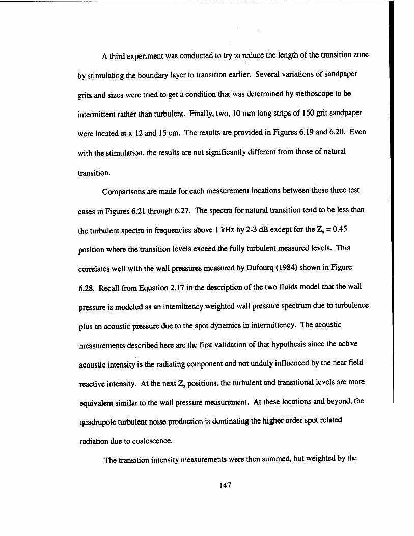
A third experiment was conducted to try to reduce the length of the transition zone
by stimulating the boundary layer to transition earlier. Several variations of sandpaper
grits and sizes were tried to get a condition that was determined by stethoscope to be
intermittent rather than turbulent. Finally, two, 10 mm long strips of 150 grit sandpaper
were located at x 12 and 15 cm. The results are provided in Figures 6.19 and 6.20. Even
with the stimulation, the results are not significantly different from those of natural
transition.
Comparisons are made for each measurement locations between these three test
cases in Figures 6.21 through 6.27. The spectra for natural transition tend to be less than
the turbulent spectra in frequencies above 1 kHz by 2-3 dB except for the Z, = 0.45
position where the transition levels exceed the fully turbulent measured levels. This
correlates well with the wall pressures measured by Dufourq (1984) shown in Figure
6.28. Recall from Equation 2.17 in the description of the two fluids model that the wall
pressure is modeled as an intemittency weighted wall pressure spectrum due to turbulence
plus an acoustic pressure due to the spot dynamics in intermittency. The acoustic
measurements described here are the first validation ofthat hypothesis since the active
acoustic intensity is the radiating component and not unduly influenced by the near field
reactive intensity. At the next Z, positions, the turbulent and transitional levels are more
equivalent similar to the wall pressure measurement. At these locations and beyond, the
quadrupole turbulent noise production is dominating the higher order spot related
radiation due to coalescence.
The transition intensity measurements were then summed, but weighted by the
147
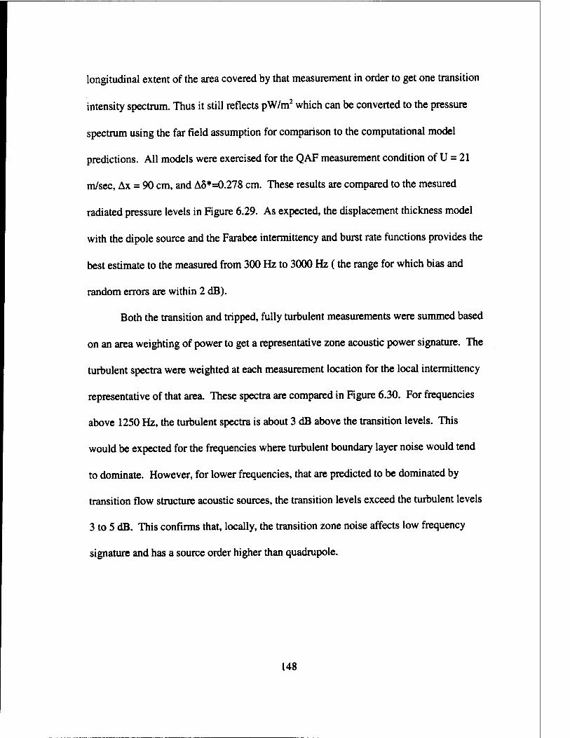
longitudinal extent of the area covered by that measurement in order to get one transition
intensity spectrum. Thus it still reflects pW/m2 which can be converted to the pressure
spectrum using the far field assumption for comparison to the computational model
predictions. All models were exercised for the QAF measurement condition of U = 21
m/sec, Ax = 90 cm, and A8*=0.278 cm. These results are compared to the mesured
radiated pressure levels in Figure 6.29. As expected, the displacement thickness model
with the dipole source and the Farabee intermittency and burst rate functions provides the
best estimate to the measured from 300 Hz to 3000 Hz (the range for which bias and
random errors are within 2 dB).
Both the transition and tripped, fully turbulent measurements were summed based
on an area weighting of power to get a representative zone acoustic power signature. The
turbulent spectra were weighted at each measurement location for the local intermittency
representative of that area. These spectra are compared in Figure 6.30. For frequencies
above 1250 Hz, the turbulent spectra is about 3 dB above the transition levels. This
would be expected for the frequencies where turbulent boundary layer noise would tend
to dominate. However, for lower frequencies, that are predicted to be dominated by
transition flow structure acoustic sources, the transition levels exceed the turbulent levels
3 to 5 dB. This confirms that, locally, the transition zone noise affects low frequency
signature and has a source order higher than quadrupole.
148
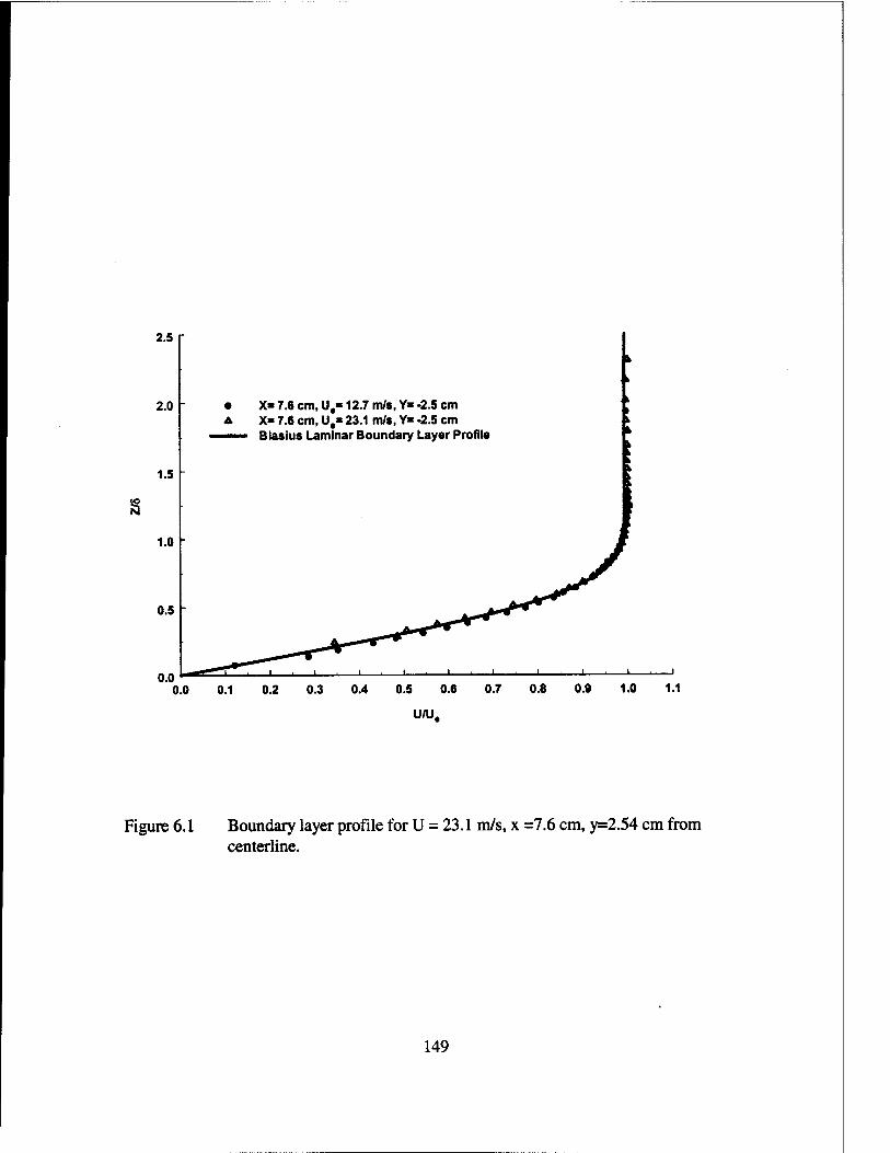
2.5
2.0
1.5
X» 7.6 cm, U,-12.7 m/s, Y- -2.5 cm X- 7.6 cm, U," 23.1 m/s, Y- -2.5 cm Blasius Laminar Boundary Layer Profil«
s
U/U,
Figure 6.1 Boundary layer profile for U = 23.1 m/s, x centerline.
=7.6 cm, y=2.54 cm from
149
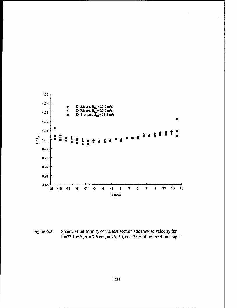
1.05
1.04
1.03
1.02
1.01
d 5 1.00 3
0.99
0.98
0.97
0.96
0.95
• Z= 3.8 cm, Ugi* 23.0 m/s A z= 7.6 cm, UCL» 23.0 m/s ■ Z» 11.4 cm, Ugi" 23.1 m/s
A • ft *
ä!5*äII* ft * f * ♦ t §
-15 -13 -11 -1 1
Y(cm)
11 13 15
Figure 6.2 Spanwise uniformity of the test section streamwise velocity for U=23.1 m/s, x = 7.6 cm, at 25,50, and 75% of test section height.
150
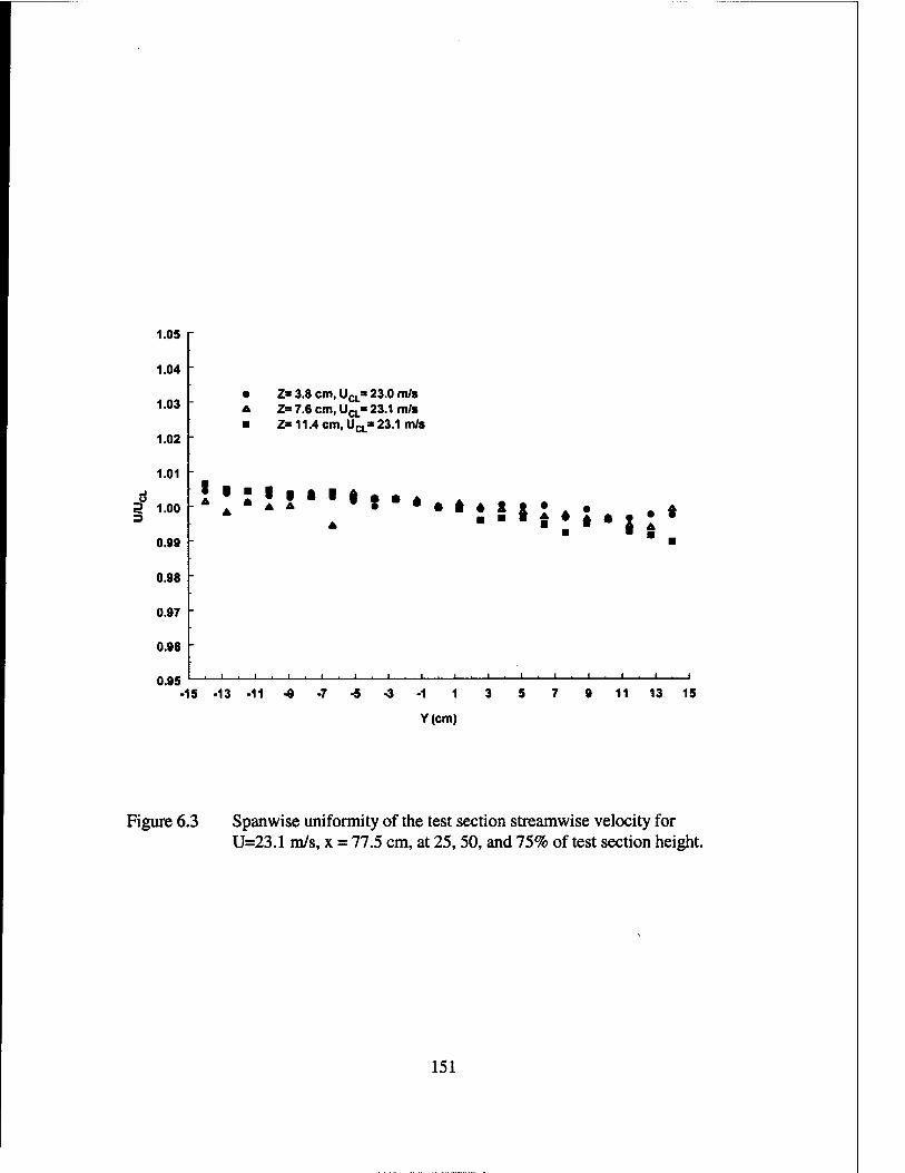
1.05
1.04
1.03
1.02
1.01
d 5 LOO
0.99
0.98
0.97
0.96
0.95
• Z* 3.8 cm, Ucj* 23.0 m/s A Z= 7.6 cm, UCL» 23.1 m/s ■ Z» 11.4 cm, UCL» 23.1 m/s
I ■ t I t t ** * I * * s: • s
-15 -13-11-9-7-5-3-1 1 3 5 7 9 11 13 15
Y(cm)
Figure 6.3 Spanwise uniformity of the test section streamwise velocity for U=23.1 m/s, x = 77.5 cm, at 25,50, and 75% of test section height.
151
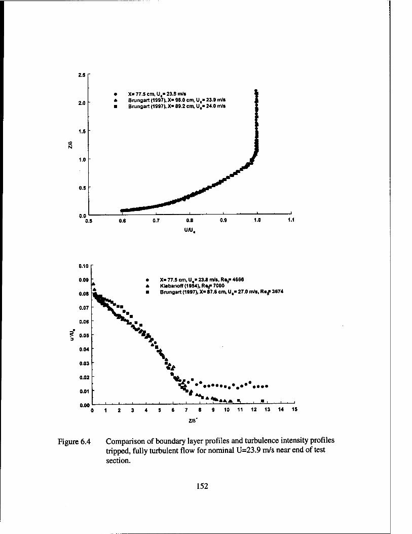
2.5
2.0
1.5
1.0
0.5
• X» 77.5 cm, Ut» 23.8 m/s A Bmngart (1997), X= 98.0 cm, Ut» 23.9 m/s ■ Brungart (1997), X« 89.2 cm, U.» 24.0 m/s
0.10
0.09 A
(
0.08 A
0.07 ,x *<■ 0.06
? 0.05 3
N, 0.04 -
0.03
0.02
0.01 -
0.00
• X-77.5 cm, Ut-23.8 m/s, RA/4666 Klsbanoff (1954), Ri^ 7000 Brungart (1997), X> 87.6 cm, Ut« 27.0 m/s, Rs,f 3674
'%
•it
_l , I i I i L.
• •••
_l , l_
0 1 2 3 4 5 6 7 8 9 10 11 12 13 14 15
278*
Figure 6.4 Comparison of boundary layer profiles and turbulence intensity profiles tripped, fully turbulent flow for nominal U=23.9 m/s near end of test section.
152
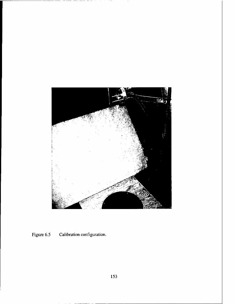
Figure 6.5 Calibration configuration.
153
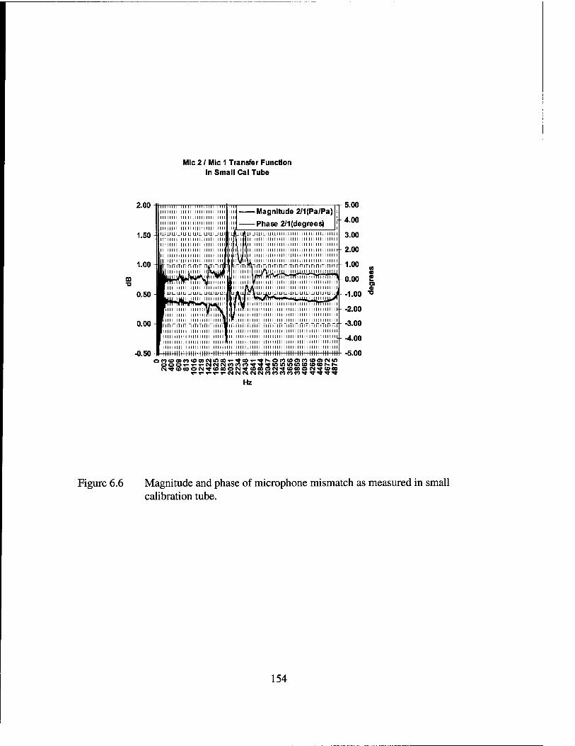
Mic 2 / Mic 1 Transfer Function In Small Cal Tube
2.00
1.50 '-
1.00
ffl
0.50
0.00
-0.50
iiiniiiiiii 11111111ni in11ill llllllllllll I I II I f I I HE I II I I ill i Magnitude 2/1(Pa/Pa) > III III111 III 11 III III III 11111 III in 111111 im i IM in i ii 11111 iii uijjuiiiu uumuiiiuuil i iiiiiiiiiiii II in in 111111 II il i
| Phase 2/1(degrees) j lAlljlimUliJUIllLIUIllULLILIiJUIllJJU ill idlll III I I I I I I II 111 II I I I I II I II I I I III I I I HH -
1111111II111111111II11111111111 llllllllllll Hill I II I I I I I I III I
Ii 11111 nun n in 111111 n i II Ii llllllllllll lllllllllllMlllfl ■rinniTin nmrimn-irinln IkliiiiiLiii Liiiiiiii|rWu|ii
III 1 lUll Ml 1 1 1 1 1 1 11 III 1 11 1 1 1 1 1 1 II llllllllllll 1 llll lllllll II 1 1 1 1 1 1 Mill 1 1 1 1 1 1 Mill llllllllllll IlilJlllS 1 11 1 1 1 II 1 II III 1 II 11 1 Ml II llllllllllll ii Vi till 11111 ii i ii in 111 ii i inn nun 111 in l n ITI mi ITI n n iTm n ITI n fT iTiTi n ITI n n MUM ll|lllj/\lUIILUJIIM^r|IJJJIIIIII|MJJ
"
Hnrmi mi 11111 rft/i 11 n 1111 Hi in in 111 M 111111 in nil II HlJJUIXIJJ UUIiJUU-ILIUI. 1 HyjjiiUJi 111111II111111111 ;
Mini 11\/TTTiiVTmiimIrrn111 niTnmnli 1 1 1 1 1 1 1 1 1 Jfll 1 1 1 III 1 1 1 1 1 Ml Ml III 1 1 HI 1 1 1 III 1 1 1 1 1 1 11 1 KjA\1!Ill II 1 1 1 1 1 II1 II1 1 111 1 1 1 1 1 1 1 111 1 1 1 u»ixjlT^iuxuj.iiJUixmuiJ-iiJUiJ.iiJLii
K!!m^T!TTipiy ! * iVii 11 II i in 11111 II i in in 11111111 Htriii 111 II i ITI 11111 n 11111111111111111111 111111111111 -
Pi 1111111111 111111111 n 11111| i "111n 111II111111111n11n11111111111u111111 In 1111 II in 11 in in i II 111 uyi
In 111 nun inniM111inuli Ii11II11111n 1111111111111111ni
iiinmiiiiiiiiiiiiiiiHiiiiii
Ml 1 II 1 Mill 1 1 1 1 1 1 II HI 1 1 1 1 1 1 1 1 1 II III 1 II 1 1 1 Ml 1 11 1 1 1 Ml 1 11 1 1 1 1 1 1 II 1 II 1 1 1 1 1 1 II 1 11 III 1 II 1 1 1 III 1 11 1 1 1 Ml 1 II 1 1 1 II 1 II 1 11 1 1 1 1 1 1 Mill III 1 II 1 1 Mil lllllll 11111II1 Ml II 1 1 1 1 1 1 III III 1 1 llllllllllll 1 1 1 1 1 1 1 11 1 1 1 1 1 1 Ml 11 1 1 1 1 1 1 III 111 1 1 111 1 1 1 Mllll
1IIIIIMIIIIIIIIIII1IIIIIIIIIH1IHHIIIIHI1II
5.00
4.00
3.00
2.00
1.00 in a 0.00 £
o -1.00 "°
-2.00
-3.00
-4.00
-5.00 OCJ<00>tO<00>CM<000^^,00^-"«h-On<DO>CO<00>CMlO ooorT-roiNNnnn^^^minininioioONN
T-T-T-^-^-t^^c^^«s«M«Mel)co«ocoe<)'*^■^■^•^■ Hz
Figure 6.6 Magnitude and phase of microphone mismatch as measured in small calibration tube.
154
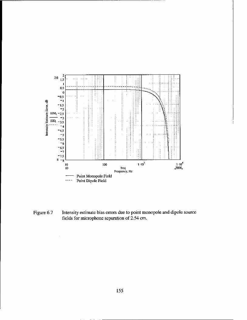
2.0 2
1.5 1
0.5 0
-0.5
@ "I
| EIMj-2.5
-3.5 -4
-4.5 "5
-5.5 "6
-6.5 "7
"7.5 i "8
EIDj
\ i ■ ; :;;■;:• ; : : ■ ■ i | \ '
; ■ ; : i i : : ; ' :\ ' '
.:.',..',;.: \ \ '■ :;:■;:! : ' \ ''
i I ■ ; ; ; i ; ; : : j '■ \ t
10 10
100 110 freq
Frequency, Hz
110 ^OOOj
Point Monopole Field Point Dipole Field
Figure 6.7 Intensity estimate bias errors due to point monopole and dipole source fields for microphone separation of 2.54 cm.
155
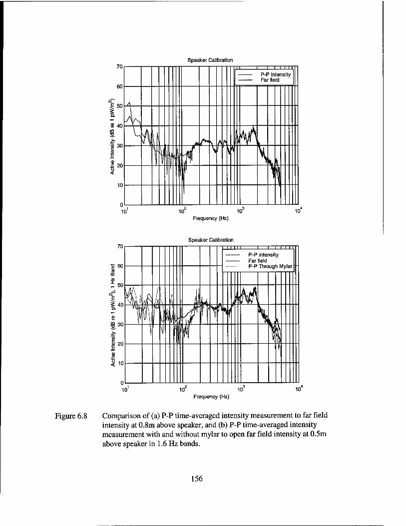
70
60
E 50
Q.
Speaker Calibration
9> m
40
'I 30
■I 20 o <
10
10 10
ii i i P-P intensity Far field
A
vL V %, £v££ MA L_ .....
W 111/ v 0
VL__... I 1 pi 1 10 10
Frequency (Hz)
Speaker Calibration
I I III
Frequency (Hz)
Figure 6.8 Comparison of (a) P-P time-averaged intensity measurement to far field intensity at 0.8m above speaker, and (b) P-P time-averaged intensity measurement with and without mylar to open far field intensity at 0.5m above speaker in 1.6 Hz bands.
156
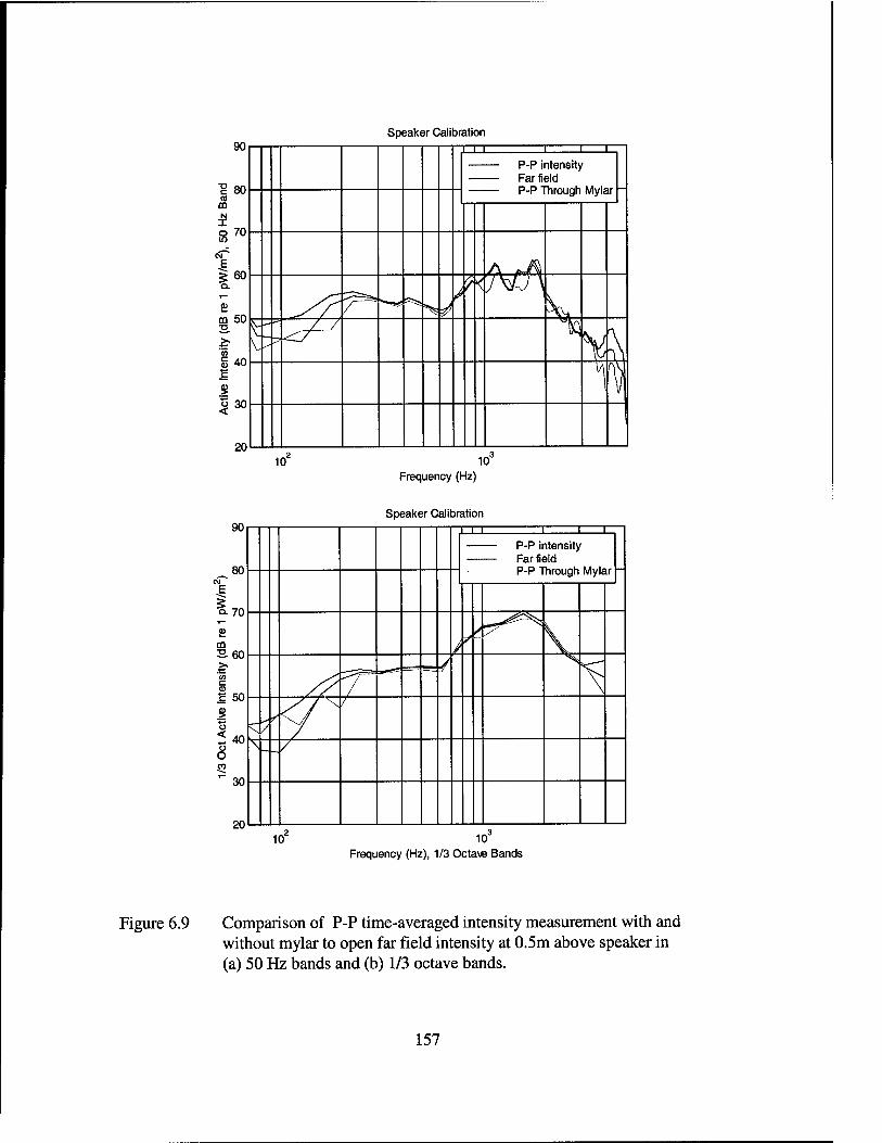
Speaker Calibration 7~T
Frequency (Hz)
Speaker Calibration
Frequency (Hz), 1/3 Octa\© Bands
Figure 6.9 Comparison of P-P time-averaged intensity measurement with and without mylar to open far field intensity at 0.5m above speaker in (a) 50 Hz bands and (b) 1/3 octave bands.
157
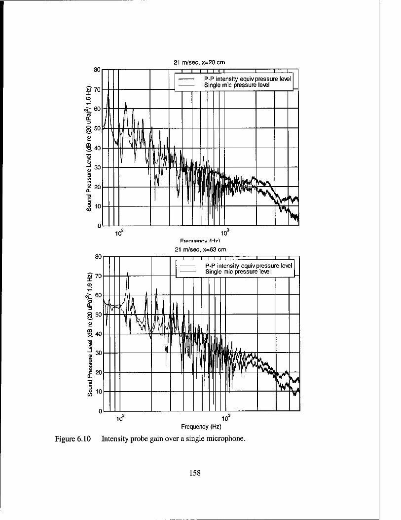
21 m/sec, x=20 cm
N X
80
70
CM
0. 3 o CM
m JO
60
50
40
30
Q.
3 O (0
20
10
Frpni ipnrw /l-+7\
21 m/sec, x=63 cm i i i i I I X I
P-P intensity equiv pressure level Single mic pressure level
Frequency (Hz)
Figure 6.10 Intensity probe gain over a single microphone.
158
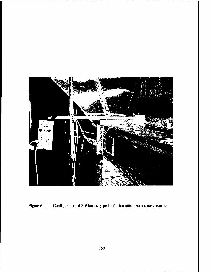
Figure 6.11 Configuration of P-P intensity probe for transition zone measurements.
159
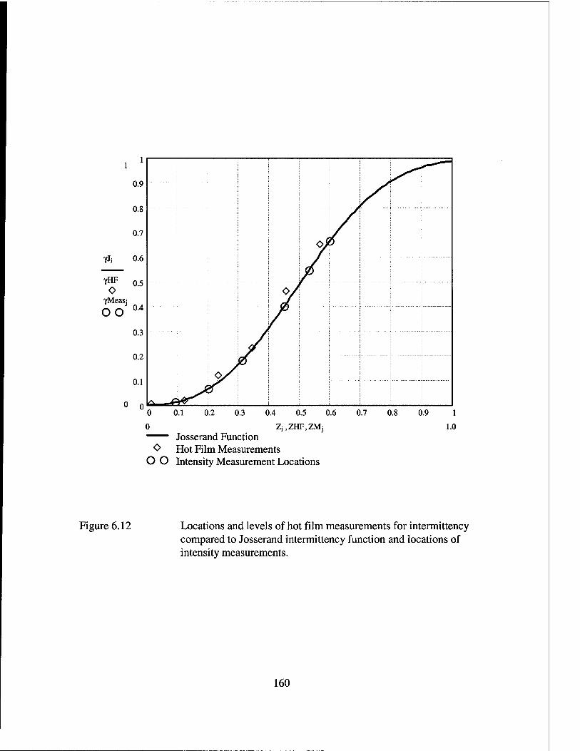
0.9
0.8
0.7
yJi 0.6
VW 0.5 o vMeaSj
o o °-4
0.3
0.2
0.1
0 0 0 0.1 0.2 0.3 0.4 0.5 0.6
0 Zi,ZHF,ZMj Josserand Function
O Hot Film Measurements O O Intensity Measurement Locations
0.7 0.8 0.9 l
1.0
Figure 6.12 Locations and levels of hot film measurements for intermittency compared to Josserand intermittency function and locations of intensity measurements.
160
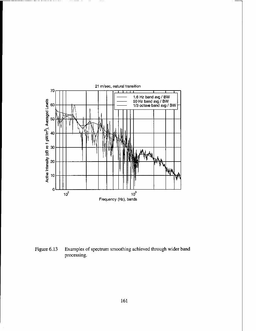
21 m/sec, natural transition 70
| 60
I 50 <
E 40
S> 30 CD ■o
w 20 c
2io <
IE I 1.6Hzbandavg/BW 50 Hz band avg / BW 1/3 octave band avg / BW
10 10 Frequency (Hz), bands
Figure 6.13 Examples of spectrum smoothing achieved through wider band processing.
161
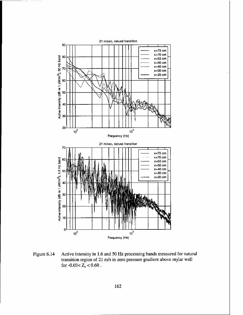
21 m/sec, natural transition
Frequency (Hz)
21 m/sec, natural transition
Frequency (Hz)
Figure 6.14 Active intensity in 1.6 and 50 Hz processing bands measured for natural transition region of 21 m/s in zero pressure gradient above mylar wall for -0.03< Zv < 0.60 .
162
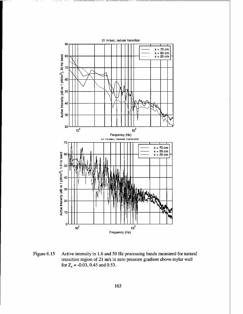
21 m/sec, natural transition
Frequency (Hz)
Figure 6.15 Active intensity in 1.6 and 50 Hz processing bands measured for natural transition region of 21 m/s in zero pressure gradient above mylar wall for Z = -0.03,0.45 and 0.53.
163
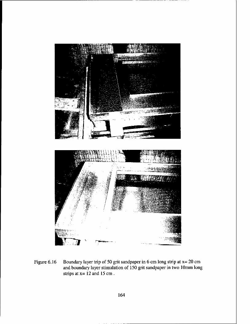
Figure 6.16 Boundary layer trip of 50 grit sandpaper in 6 cm long strip at x= 20 cm and boundary layer stimulation of 150 grit sandpaper in two 10mm long strips at x= 12 and 15 cm .
164
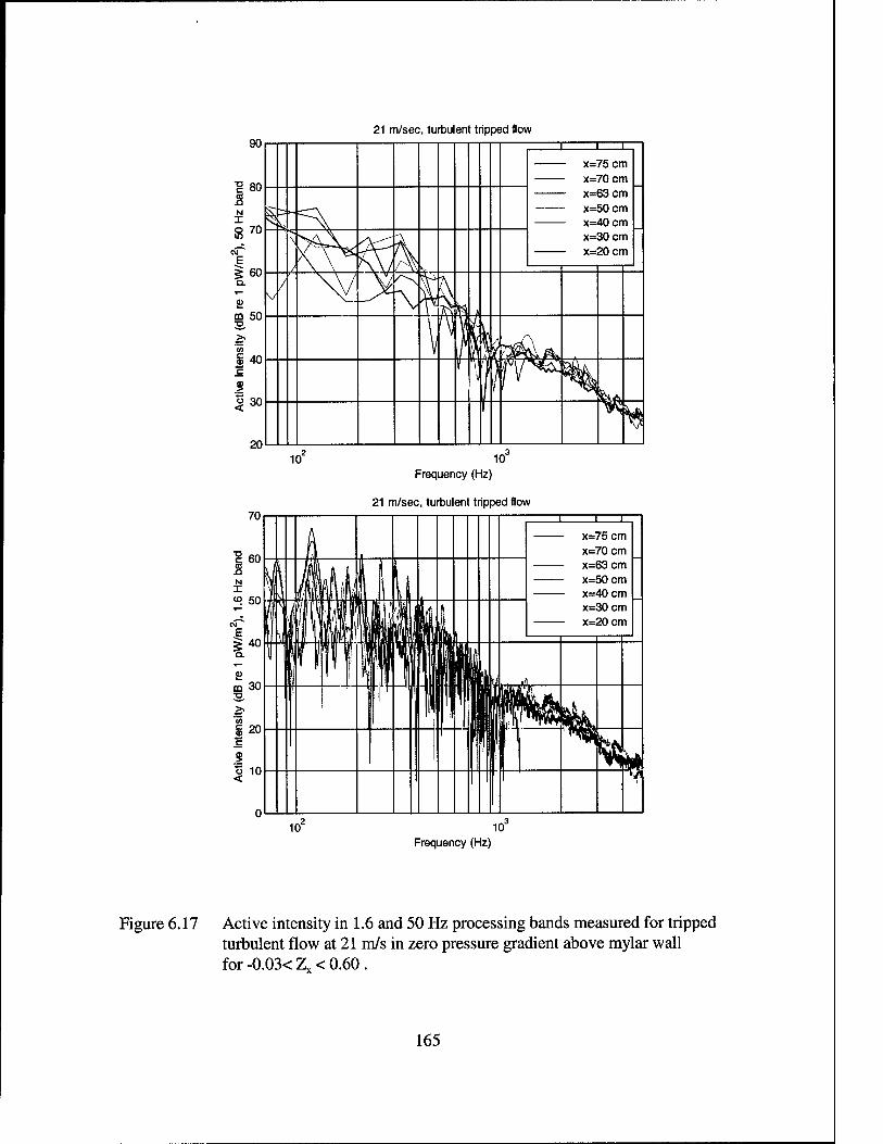
90 21 m/sec, turbulent tripped flow
■o c s N X 8
80
70
60
50
40
I o < 30
20
i i i
x=75 cm x=70 cm x=63 cm x=50 cm x=40 cm
x=30 cm x=20 cm
f Kv /^ K
/ V ^
\ ^
M
\ H \fl
K />^*^W ^iv
\ f jfr^
10 10 Frequency (Hz)
21 m/sec, turbulent tripped flow
Frequency (Hz)
Figure 6.17 Active intensity in 1.6 and 50 Hz processing bands measured for tripped turbulent flow at 21 m/s in zero pressure gradient above mylar wall for -0.03< Zx < 0.60 .
165
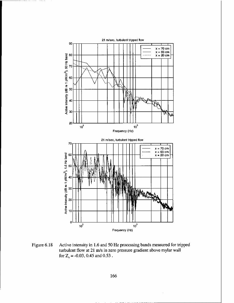
90
"g 80 S N I
21 m/sec, turbulent tripped flow
s 70
60
m 2, >.
"<5 c
c
■I ü <
50
40
30
20
i i i
x = 70 cm x = 63 cm x = 20 cm
^
^ ̂ \ \
/ V V
\ % ^ l
ß |o^/** V ' )/r* ̂
i ^
10 10 Frequency (Hz)
21 m/sec, turbulent tripped flow
Frequency (Hz)
Figure 6.18 Active intensity in 1.6 and 50 Hz processing bands measured for tripped turbulent flow at 21 m/s in zero pressure gradient above mylar wall for Z=-0.03,0.45 and 0.53.
166
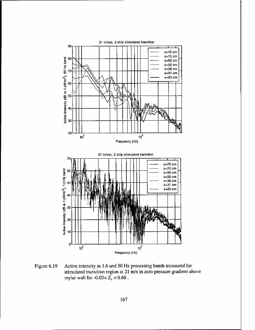
21 m/sec, 2 strip stimulated transition
70
60
N I <° 50
E 5 40 Q.
£ m 30 2. >.
'55 § 20 'S
10
Frequency (Hz)
21 m/sec, 2 strip stimulated transition i i i
I I
\
ülfil I «Mil x=31 xm
H flUlffl« iB lillHIR llfly TjMltl
|rjffl
111 ill
| 1 ill *%m
I ■r '^JtV
. Ill
10' 10 Frequency (Hz)
Figure 6.19 Active intensity in 1.6 and 50 Hz processing bands measured for stimulated transition region at 21 m/s in zero pressure gradient above mylar wall for -0.03< Zx < 0.60 .
167
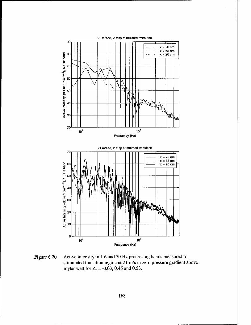
21 m/sec, 2 strip stimulated transition
Frequency (Hz)
21 m/sec, 2 strip stimulated transition
Frequency (Hz)
Figure 6.20 Active intensity in 1.6 and 50 Hz processing bands measured for stimulated transition region at 21 m/s in zero pressure gradient above mylar wall for Zx = -0.03,0.45 and 0.53.
168
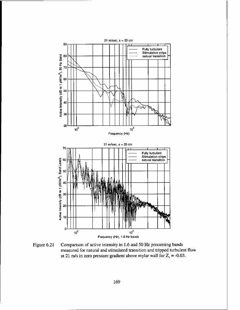
21 m/sec, x = 20 cm 90
ID C ra m N I s
80
70
E 5 60
m 50 p.
c
3 ü 30 <
20
i,,
II III
Fully turbulent Stimulation strips
natural transition - \ \
\^
V- > /—■ X \
V 1 \ /■
\ /^
/ 1
X >\
%
10 10 Frequency (Hz)
21 m/sec, x = 20 cm
IX
Frequency (Hz), 1.6 Hz bands
Figure 6.21 Comparison of active intensity in 1.6 and 50 Hz processing bands measured for natural and stimulated transition and tripped turbulent flow at 21 m/s in zero pressure gradient above mylar wall for Zx = -0.03.
169

21 m/sec, x = 30 cm 90
c a m N x s
80
70
i ffl ;o >> 'S c ID
60
50
40
30
20
-1-1— 1 1 1
Fully turbulent Stimulation strips natural transition -
^ \
*\\ /\ / ^
\.
^ i X \||U\ \§&>* -v
t^V I V ^
10' 10 Frequency (Hz)
21 m/sec, x = 30 cm
Frequency (Hz), 1.6 Hz bands
Figure 6.22 Comparison of active intensity in 1.6 and 50 Hz processing bands measured for natural and stimulated transition and tripped turbulent flow at 21 m/s in zero pressure gradient above mylar wall for Zx = 0.09.
170
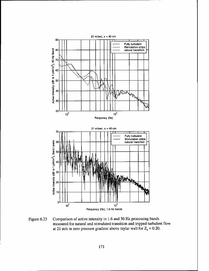
21 m/sec, x = 40 cm 90
« CD N I O m
80
70
E g 60
CO 50 ■o
40
30
20
M iii
Fully turbulent Stimulation strips
\
V-
V^ \ A h V V f\ \ \\"s^ \n^ X ̂
\
10 10 Frequency (Hz)
21 m/sec, x
Frequency (Hz), 1.6 Hz bands
Figure 6.23 Comparison of active intensity in 1.6 and 50 Hz processing bands measured for natural and stimulated transition and tripped turbulent flow at 21 m/s in zero pressure gradient above mylar wall for Zx = 0.20.
171
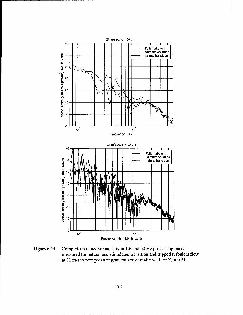
21 m/sec, x = 50 cm X
Frequency (Hz)
21 m/sec, x = 50 cm
Frequency (Hz), 1.6 Hz bands
Figure 6.24 Comparison of active intensity in 1.6 and 50 Hz processing bands measured for natural and stimulated transition and tripped turbulent flow at 21 m/s in zero pressure gradient above mylar wall for Zx = 0.31.
172
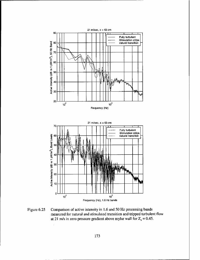
21 m/sec, x
Frequency (Hz)
21 m/sec, x = 63 cm
XT
Frequency (Hz), 1.6 Hz bands
Figure 6.25 Comparison of active intensity in 1.6 and 50 Hz processing bands measured for natural and stimulated transition and tripped turbulent flow at 21 m/s in zero pressure gradient above mylar wall for Zx = 0.45.
173
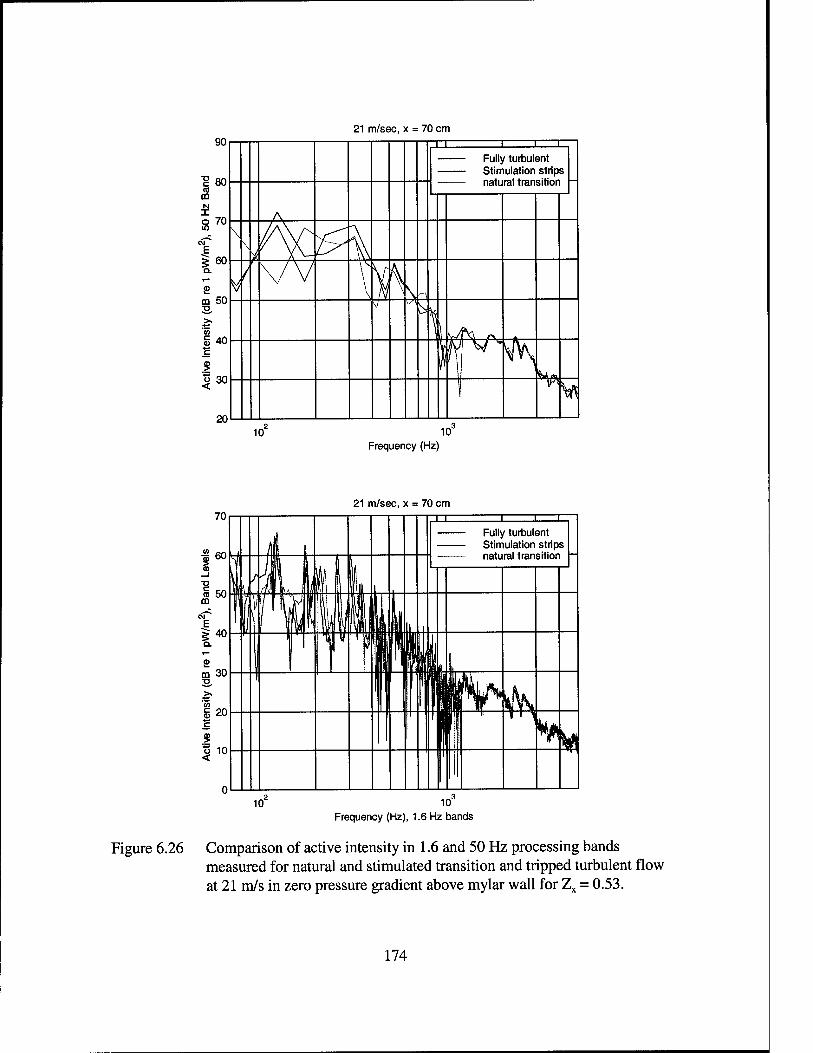
21 m/sec, x = 70 cm 90
c « m N I s
80
70
60
ffl >. 55 c
50
40
30
20
11 Fully turbulent Stimulation strips
A
\^C H k /vv \ i \^ \i d
WWV\
***
10 10 Frequency (Hz)
21 m/sec, x = 70 cm
Frequency (Hz), 1.6 Hz bands
Figure 6.26 Comparison of active intensity in 1.6 and 50 Hz processing bands measured for natural and stimulated transition and tripped turbulent flow at 21 m/s in zero pressure gradient above mylar wall for Zx = 0.53.
174
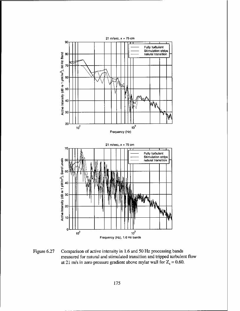
21 m/sec, x = 75 cm
Frequency (Hz)
21 m/sec, x = 75 cm H
Frequency (Hz), 1.6 Hz bands
Figure 6.27 Comparison of active intensity in 1.6 and 50 Hz processing bands measured for natural and stimulated transition and tripped turbulent flow at 21 m/s in zero pressure gradient above mylar wall for Zx = 0.60.
175
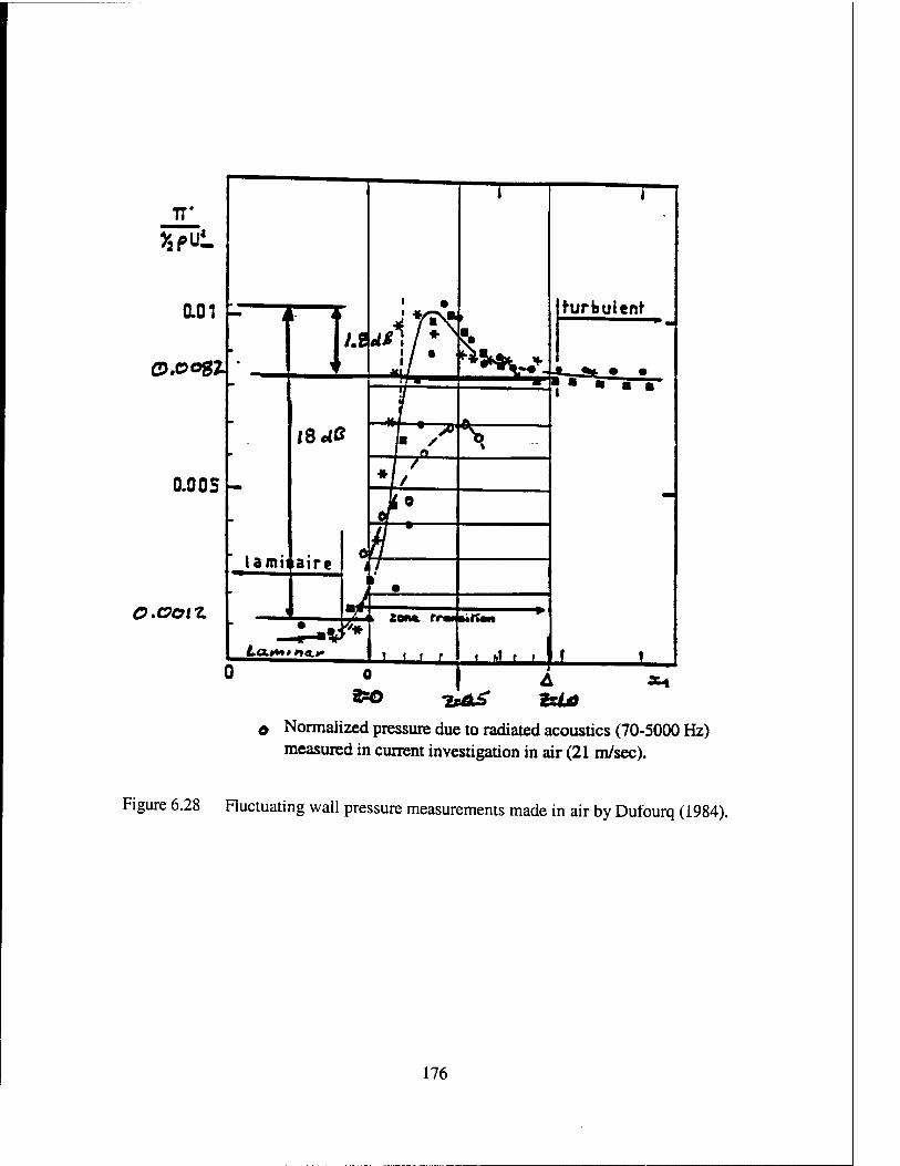
o.ootz
Q Normalized pressure due to radiated acoustics (70-5000 Hz) measured in current investigation in air (21 m/sec).
Figure 6.28 Fluctuating wall pressure measurements made in air by Dufourq (1984).
176
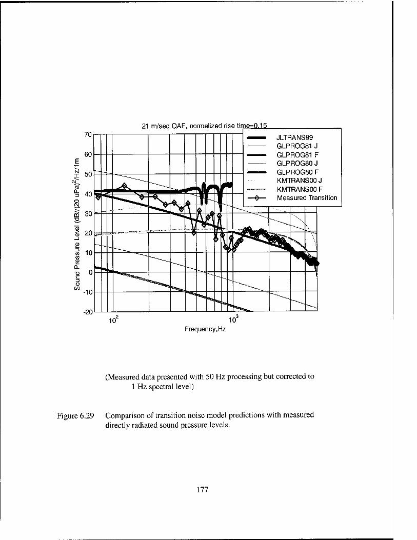
m/sec QAF, normalized rise time=0.15
N X
Q.
O CM
CO
CD _l
CO CO CD
T3 c o
Frequency,Hz
(Measured data presented with 50 Hz processing but corrected to 1 Hz spectral level)
Figure 6.29 Comparison of transition noise model predictions with measured directly radiated sound pressure levels.
177
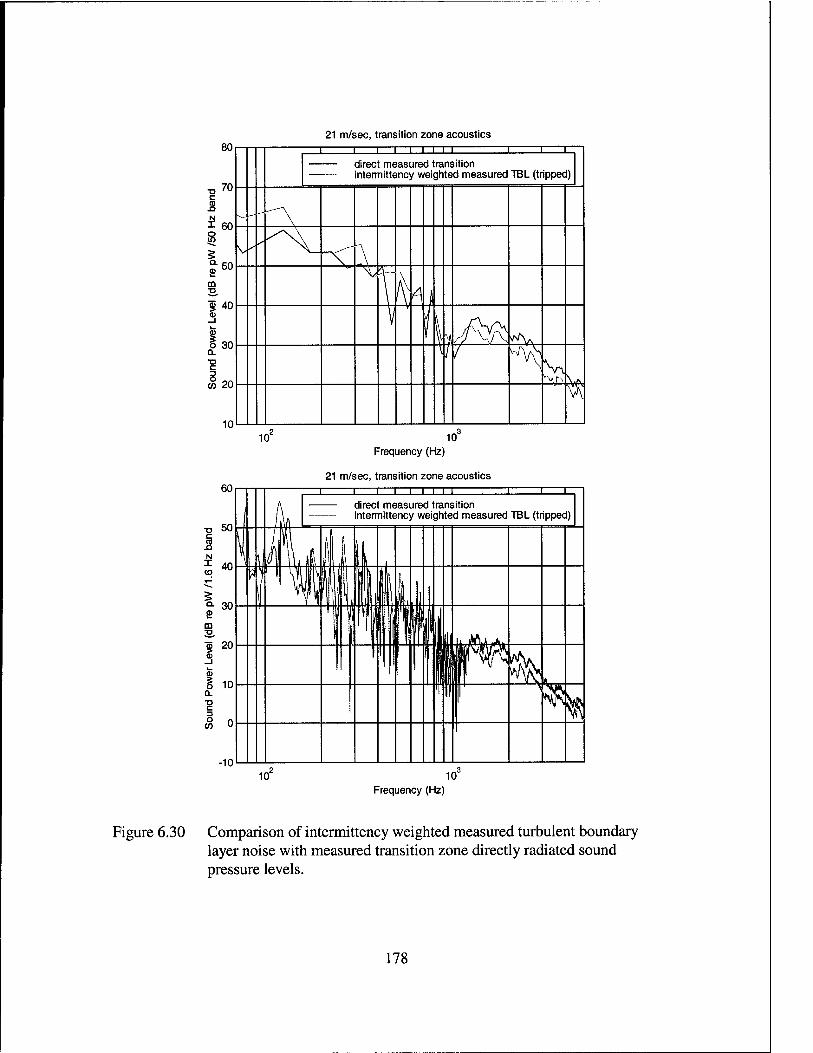
21 m/sec, transition zone acoustics 80
•D C
& N I s I s m
9
70
60
50
40
30
(§20
10
X in r direct measured transition intermittency weighted measured TBL (tripped)
10 10 Frequency (Hz)
21 m/sec, transition zone acoustics
Frequency (Hz)
Figure 6.30 Comparison of intermittency weighted measured turbulent boundary layer noise with measured transition zone directly radiated sound pressure levels.
178
CHAPTER 7
CONCLUSIONS AND FUTURE WORK
7.1 Conclusions
The research described in this dissertation has resulted in the following unique
contributions and conclusions.
1. First unambiguous direct measurement of the acoustic radiation from a boundary
layer transition zone.
2. Confirmed that the wall pressure peak measured by Dufourq (1984) in the range
0.4 < Z, < 0.55 under a transition zone is due to the radiated acoustic pressure.
3. The acoustic theory developed by Lauchle using the Liepmann fluctuating
displacement thickness approach, and an infinite flat plate Green's function with
monopole source field appears to be incorrect when compared against the
measurements. Lauchle's model has been improved by using a dipole source field
based on the Krane (1992) water channel data, and on qualitative observations of
the flow structures present during transition. The true axis angle of the dipole
relative to the wall has yet to be determined. There may even be an occurrence of
multiple angles in a natural transition zone.
4. Rather than using a constant dipole axis (source separation distance), which
results in unrealistic high-frequency content of the predicted transition noise
(extensive sinusoidal null variation in levels), a statistical estimate is constructed
by treating the dipole axis as a random variable. This variable is assumed
179
uniformly distributed over physically predictable limits. This results in a
smoothed spectral estimate and better match with the measured data. This
prediction model provides the best fit to the measured data for frequencies above
300 Hz. Because of measurement uncertainty, a proper comparison cannot be
made below that frequency at this time. In addition, the angle of the dipole may
vary depending on the growth dynamics of the turbulent spot. A treatment similar
to the one described for dipole source separation distance in section 3.1.2 could
also be incorporated for this dipole axis angle.
5. Demonstrated that the intermittency-weighted, fully turbulent boundary layer
radiated sound power level is a good approximation to the directly radiated sound
power level from the transition zone. The level was found to be about 3 dB below
that of the transition zone noise for f < 1 kHz .and 3 dB high for f > 1 kHz.
6. The two-fluids model proposed by Lagier and Sornette offers no real prediction
benefit over the Lauchle model once the spatial dependence is brought back inside
the integral and given the simplifications that were necessary to make the two
fluids model integrable.
7.2 General Observations on Transition Noise
The following are observations that have resulted from the cumulative knowledge
gained over the course of this research including the background materials and
understanding of the previous works of others.
1. Most of the focus in boundary layer transition acoustics in the last eight years has
180
been on developing direct numerical simulation (DNS) approaches to modeling
using spatial and temporal approaches to solving the complete Navier-Stokes
equations. Based on the results of Wang, et al. (1996), there appears to be more
"noise" in the calculation than is produced by the actual fluid dynamics. However,
the value of DNS may really be to provide insight on the necessary modeling of
substructure dynamics that influence the spatial definition of the normal velocity
used in the fluctuating displacement thickness model and contribute in their own
right to the acoustic pressure particularly influencing the near-field. This bridges
the gap to some extent between the two fluids model using the Lighthill analogy
and the Liepmann approach used for the fluctuating displacement thickness
model.
2. The predicted low frequency contribution of transition noise seems to be
significant, particularly for f <300 Hz and higher mean flow velocities. Audet et
al. (1989a, Figure 10) show this as a domination of the low polar order growth
mechanism of the spot (a la Lauchle) over the quadrupole source due to the TBL
statistics in the turbulent spots. Howe's model (1999) for the effect of a transition
zone near the leading edge of a hydrofoil clearly show an enhancement of the
same low frequency regime due to the transition zone.
3. Laboratory measurements performed prior to this dissertation indicate that
transition zone noise levels may be contaminated by other sources. It is suspected
that one contaminating source for early measurements in this investigation (with
an early QAF configuration) was trailing edge noise when a jet was discharging
181
across a flat plate. However, the axisymmetric body tests by Perraud (1989)
indicated propagation of acoustic noise from the transition region to sensors in the
laminar flow zone. The results reported here qualitatively supports this finding.
Transition in an adverse pressure gradient will result in higher radiated and
structural excitation levels in comparison to transition in a zero pressure gradient.
Huang and Shen (1989) found wall pressure levels 2 to 3 times higher for
transition in adverse pressure gradients compared to TBL wall pressure levels.
Mautner and Van Atta (1982) found rms wall pressures for individual turbulent
spots to be 0.010-0.015 of dynamic pressure Q/i QU02) for zero and favorable
pressure gradients and 0.015-0.030 of dynamic pressure in adverse gradients.
More importantly, in the adverse gradient, the wall pressure spectrum was nearly
constant magnitude with increasing frequency rather than the typical decreasing
slope. This is enhanced further if transition is induced by laminar boundary layer
separation and re-attachment. In particular, Huang and Shen found that wall
pressures in reattachment zones for laminar separation were 10 to 15 times higher.
Hwang and Shang (1989) and Hwang and Maidanik (1990) have worked on
approaches for modeling the coupling of these wall pressures within transition
zones with the underlying structure.
The preceding observation is perhaps what should command our continued
interest because of the engineering relevance associated with forebodies of bodies
of revolution and for airfoil leading edges where acoustic sources may be located.
Just as trailing edge flows are critical to the direct radiation, excitation, re-
182
radiation and scattering of noise at airfoil trailing edges (see Brooks and Hodgson,
1981 and Gershfeld, 1997), so may transition near the leading edge of an airfoil
act as a noise source. Of course, this is quite dependent upon the chordwise
distribution of thickness for the airfoil and the local radii of curvature (Howe,
1981).
7.3 Recommended Future Work
The recommendations for future work are as follows.
• CFD Validation - More experimental data will be needed at increasing Reynolds
numbers to validate the computational fluid dynamics solution approaches using
Reynolds Averaged Navier-Stokes (RANS) or Large Eddy Simulation (LES)
• Transition Noise in Adverse Pressure Gradients - Radiated noise and fluid
mechanics measurements need to be made for a systematic variation of adverse
pressure gradient. Pursuit of further modeling or measurement of zero pressure
gradient flows does not seem warranted based on the small contribution to the
overall flow-induced radiated noise for a flat plate. However, the indications are
that adverse pressure gradients should shorten the transition zone and, thus, result
in a higher radiated noise component.
• Transition on Blades - Radiated noise due to boundary layer transition on air- and
hydrofoils is a topic of continued interest. The usefulness of the models described
in this thesis when coupled with the proper Green's function should be evaluated
against measurements. But, it is noted that the mechanism for transition on blades
183
is often a bypass phenomenon or a result of separation.
Experimental Validation - Continue to utilize the current Quiet Airflow Facility to
measure the radiation from the leading edge of the existing a half-plane foil in the
presence of various pressure gradients, particularly adverse. Also, perform similar
experiments on axisymmetric headforms.
Coherent Output Intensity - This procedure should continue to be pursued with a
better implementation of the real-time intensity circuitry. The concept of using a
sensor unaffected by the acoustic field to condition the intensity measurement is very
powerful.
184
BIBLIOGRAPHY
Abraham, B. M. and Keith, W. L., 1997, "Wavenumber Spectra of High Magnitude Wall Pressure Events in a Numerically Simulated Turbulent Boundary Layer," Trans. ASME, J. Fluids Eng. 119, pp. 281-288.
Addison, J. S. and Hodson, H. P., 1991, "Modelling of Unsteady Transitional Boundary Layers," Paper 91-GT-282, ASME International Gas Turbine and Aeroengine Congress and Exhibition, Orlando, FL, June 1991.
Arakeri, V. H., 1975, "A Note on the Transition Observations on an Axisymmetric Body and Some Related Fluctuating Wall Pressure Measurements," Trans. ASME, J. Fluids Eng,. 97, pp. 82-86.
Arakeri, V. H, Satyanarayana, S. G., Mani, K. and Sharma, S. D., 1991, "Studies on Scaling of Flow Noise Received at the Stagnation Point of an Axisymmetric Body," J. Sound Vib. 146, pp. 449-462.
Assessment of Experimental Uncertainty with Application to Wind Tunnel Testing, 1999, American Institute of Aeronautics and Astronautics (AIAA) Standard S-071A-1999, Reston, VA.
Audet, J., Dufourq, Ph. and Lagier, M., 1989a, "Pression parietale sous une couche limite Lore de la transition vers la turbulence," J. Acoustique 2: pp. 369-378. (Translation available: Marboe, R. C, Applied Research Laboratory / Penn State University Tech. Memo. 91-81,5 April 1991.)
Audet, J., Dufourcq, Ph., Lagier, M. and Sornette, D., 1989b, "Wall Pressure Fluctuations in the Intermittent Regime of a Transition Boundary Layer Comparison Between Theory and Experiment," Symposium on Flow- Induced Noise due to Laminar-Turbulence Transition Process, (Farabee, T. M., Hansen, R. J. and Keltie, R. F., eds.), ASME NCA-Vol. 5, pp. 25-30.
Bandyopadhyay, P. R. and Ahmed, A., 1993, "Turbulent Boundary Layers Subjected to Multiple Curvatures and Pressure Gradients," J. Fluid Mech. 246, pp. 503-527.
Barenblatt, G. I., 1990, "On a Model of Laminar-Turbulent Transition," J. Fluid Mech. 212, pp. 487-496.
185
Barker, S. J., 1974, "Measurements of Radiated Noise in the CALTECH High-Speed Water Tunnel, Part 1: Radiated Noise from Turbulent Boundary Layers," Graduate Aeronautical Laboratories Report, California Institute of Technology, Pasadena, CA, 30 August 1974.
Barlow, J. B., Rae, W. HM Jr., and Pope, A., 1999, Low-Speed Wind Tunnel Testing, 3rd Ed., John Wiley and Sons, New York.
Barrow, J., Barnes, F. H., Ross, M. A. S., and Hayes, S. T., 1984, "The Structure of a Turbulent Spot in Blasius Flow," /. Fluid Mech. 149, pp. 319-337.
Bendat, J. S. and Piersol, A. G., 1993, Engineering Applications of Correlation and Spectral Analysis, Second Edition, John Wiley & Sons, New York, Chapter 4.
Beranek, L. L., 1988, Noise and Vibration Control, Revised Edition, Institute of Noise Control Engineering, Washington, DC, pp. 575.
Bergeron, R. F., 1973, "Aerodynamic Sound and Low Wavenumber Wall-Pressure Spectrum of Nearly Incompressible Boundary Layer Turbulence," /. Acoust. Soc. Am. 54, pp. 123-133.
Bershadskii, A. and Tsinober, A., 1994, "On the Near Field Pressure Radiation and Localized Structures in Turbulence," /. Sound Vib. 173, pp. 699-701.
Blair, M. F., 1992a, "Boundary-Layer Transition in Accelerating Flows With Intense Freestream Turbulence: Part 1 - Disturbance Upstream of Transition Onset," Trans. ASME, J. Fluids Eng. 114, pp. 313-321.
Blair, M. F., 1992b, "Boundary-Layer Transition in Accelerating Flows With Intense Freestream Turbulence: Part 2 - The Zone of Intermittent Turbulence," Trans. ASME, J. Fluids Eng. 114, pp. 322-332.
Blake, W. K., 1986, Mechanics of Flow-Induced Sound and Vibration, Volumes I and II, Academic Press, Orlando, Chapters 2,9, and 11.
Bowles, R. G. A. and Smith, F. T., 1995, "Short-Scale Effects on Model Boundary-Layer Spots," / Fluid Mech. 295, pp. 395-407.
Brooks, T. F. and Hodgson, T. H., 1981, "Trailing Edge Noise Prediction from Measured Surface Pressures," J. Sound Vib. 78, pp. 69-117.
186
Bruneau, S. D. and Pauley, W. R., 1992, "Digital Image Processing of Hydrogen Bubble Lines for Instantaneous Velocity Profiles," Applied Research Laboratory / Penn State University Tech. Report 92-10, November 1992.
Bruneau, S. D. and Pauley, W. R., 1995, "Measuring Unsteady Velocity Profiles and Integral Parameters Using Digital Image Processing of Hydrogen Bubble Timelines," Trans. ASME, J. Fluids Eng. 117, pp. 331-340.
Brungart, T. A., 1997, "Boundary Condition Effects on Turbulent Boundary Layer Wall Pressure Fluctuations," Ph.D. Thesis in Acoustics, The Pennsylvania State University, December 1997.
Capone, D. E. and Lauchle, G. C, 1995, "Calculation of Turbulent Boundary Layer Wall Pressure Spectra," J. Acoust. Soc. Am. 98: pp. 2226-2234.
Chase, D. M, 1980, "Modeling the Wavevector-Frequency Spectrum of Turbulent Boundary Layer Wall Pressure," J. Sound Vib. 70, pp. 29-47.
Chase, D. M., 1987, "The Character of the Turbulent Wall Pressure Spectrum at Subconvective Wavenumbers and a Suggested Comprehensive Model," J. Sound Vib. Ill, pp. 125-142.
Chase, D. M., 1989, private communication.
Chase, D. M., 1991, "The Wave-Vector-Frequency Spectrum of Pressure on a Smooth Plane in Turbulent Boundary-Layer Flow at Low Mach Number," J. Acoust. Soc. Am. 90, pp. 1032-1040.
Chen, K. K. and Thyson, N. A., 1971, "Extension of Emmons' Spot Theory to Flows on Blunt Bodies," A1AA J. 9, pp. 821-825.
Chernys, M. and Pauley, W. R., 1994, "The Effect of Interaction Strength on the Development and Acoustic Signature of Aligned Turbulent Spot Pairs," Symposium on Boundary Layer and Free Shear Flows, (Donovan, J. F. and Dutton, J. C, eds.), ASME FED-Vol. 184, pp. 21-35.
Ching, C. Y. and LaGraff, J. E., 1995, "Measurement of Turbulent Spot Convection Rates in a Transitional Boundary Layer," Exper. Thermal and Fluid Sei., 11, pp. 52-60.
Clark, J. P., Jones, T. V., and LaGraff, J. E., 1996, "Turbulent Spot Propagation in a Decelerating, Compressible Flow," Trans. ASME, J. Fluids Eng,. 118, pp. 612-614.
187
Coleman, H. W. and Steele, W. G., 1999, Experimentation and Uncertainty Analysis for Engineers, 2nd Ed., John Wiley and Sons, New York.
Coles, D, and Savas, O., 1979, "Interactions for Regular Patterns of Turbulent Spots in a Laminar Boundary Layer," In Proc. IUTAM Symposium Laminar-Turbulent Transition, Stuttgart, Germany, September 16-22,1979, Springer-Verlag, Berlin, pp. 277-287.
Corcos, G. M., 1963, "Resolution of Pressure in Turbulence," /. Acoust. Soc. Am. 35, pp. 192-199.
Crighton, D. G., 1975, "Basic Principles of Aerodynamic Noise Generation," Prog. Aerosp. Sei., 16, pp. 31-39.
Curie, N., 1955, "The Influence of Solid Boundaries Upon Aerodynamic Sound," Proc. Royal Soc. London A, 231, pp. 505-514.
DeMetz, F. C. and Casarella, M. J., 1973, "An Experimental Study of the Intermittent Properties of the Boundary Layer Pressure Field During Transition on a Rat Plate," David W. Taylor Naval Ship Research and Development Center Report AD-775-299, November 1973.
Dey, J. and Narasimha, R., 1991, "Effect of Favorable Pressure Gradient on Transitional Spot Formation Rate," Exper. Thermal and Fluid Sei. 4, pp. 192-197.
Dhawan, S. and Narasimha, R., 1958, "Some Properties of Boundary Layer Flow During The Transition from Laminar to Turbulent Motion," J. Fluid Mech. 3, pp. 318-436.
Ducros, F., Comte, P., and Lesieur, M., 1996, "Large-Eddy Simulation of Transition to Turbulence in a Boundary Layer Developing Spatially Over a Rat Plate," J. Fluid Mech. 326, pp. 1-36.
Dufourq, Ph.,1984, "Influence d'un 6coulement de Type Couche Limite sur la Localisation de Sources Sonores Placees en Paroi," Doctoral Thesis, Ecole Centrale de Lyon.
Emmons, H. W., 1951, "The Laminar-Turbulent Transition in a Boundary-Layer, Part 1/7. Aeron. Sei. 18, pp. 490-498.
Fahy, F. J., 1989, Sound Intensity, Elsevier Applied Science, New York
Farabee, T. M., Casarella, M. J., and DeMetz, F. C, 1974, "Source Distribution of Turbulent Bursts During Natural Transition," David W. Taylor Naval Ship Research and Development Center Report SAD-89E-1942, August 1974.
188
Ffowcs Williams, J. R, 1967, "Flow Noise," Underwater Acoustics, Vol. II, Alters, V. M. (ed), Plenum Press.
Ffowcs Williams, J. E., 1969, "Hydrodynamic Noise," Ann. Rev. Fluid Meek 1, pp. 197- 221.
Ffowcs Williams, J. E., 1977, "Aeroacoustics," Ann. Rev. Fluid Mech. 9, pp. 447-468.
Ffowcs Williams, J. E., 1982, "Noise Source Mechanisms in Unsteady Flow," Acustica 50, pp. 167.
Gad-el-Hak, M., 1989, "Flow Control," Appl. Mech. Rev. 42, pp. 261.
Gad-el-Hak, M., Blackwelder, R. F. and Riley, J. J., 1981, "On the Growth of Turbulent Regions in Laminar Boundary Layers," J. Fluid Mech, 110, pp. 73-95.
Gad-el-Hak, M. and Fazle Hussain, A. K. M., 1986, "Coherent Structures in a Turbulent Boundary Layer, Part 1: Generation of 'Artificial' Bursts," Phys. Fluids 29, pp. 2124-2138.
Gedney, C. J., 1979, "Wall Pressure Fluctuations During Transition on a Flat Plate," Mass. Institute of Tech. Report 84618-1.
Gedney, C.J. and Leehey, P., 1989, "Wall Pressure Fluctuations During Transition on a Flat Plate," Symposium on Flow-Induced Noise Due to Laminar-Turbulence Transition Process, (Farabee, T. M., Hansen, R. J. and Keltie, R. F., eds.), ASME NCA-Vol. 5, pp. 1-10.
Gershfeld, J. L., 1997,"Sound Generation from Spatially Inhomogeneous Wall Pressure Fields (Polyvinylidene Fluoride)," Ph.D. Thesis, The Catholic University of America, August 1997.
Gogineni, S. and Shih, C, 1997, "Experimental Investigation of the Unsteady Structure of a Transitional Plane Wall Jet," Exper. in Fluids 23, pp. 121-129.
Goldstein, M. E., Leib, S. J. and Cowley, S. J., 1992, "Distortion of a Flat-Plate Boundary Layer by Free-Stream Vorticity Normal to the Plate, '7. Fluid Mech. 237, pp. 231-260.
Goldstein, M. E. and Leib, S. J., 1993, "Three-Dimensional Boundary-Layer Instability and Separation Induced by Small-Amplitude Streamwise Vorticity in the Upstream Row," J. Fluid Mech. 246, pp. 21-41.
189
Graham, W. R., 1997, "A Comparison of Models for the Wavenumber-Frequency Spectrum of Turbulent Boundary Layer Pressures," J. Sound Vib. 206, pp. 541-565.
Gutmark, E. and Blackwelder, R. F., 1987, "On the Structure of a Turbulent Spot in a Heated Laminar Boundary Layer," Exper. in Fluids 5, pp. 217-229.
Haddle, G. P. and Skudrzyk, E. J., 1969, "The Physics of How Noise," J. Acoust. Soc. Amer. 46, pp. 130-157.
Haidari, A. H. and Smith, C. R., 1994, "The Generation and Regeneration of Single Hairpin Vortices," J. Fluid Meek 277, pp. 135-162.
Halstead, D. E., Wisler, D. C., Okiishi, T. H., Walker, G. J., Hodson, H. P. and Shin, H. W., 1995a, "Boundary Layer Development in Axial Compressors and Turbines, Part 1 of 4: Composite Picture," Paper 95-GT-461, ASME International Gas Turbine and Aeroengine Congress and Exhibition, Houston, TX, June 1995.
Halstead, D. E., Wisler, D. C, Okiishi, T. H., Walker, G. J., Hodson, H. P. and Shin, H. W., 1995b, "Boundary Layer Development in Axial Compressors and Turbines, Part 2 of 4: Compressors," Paper 95-GT-462, ASME International Gas Turbine and Aeroengine Congress and Exhibition, Houston, TX, June 1995.
Halstead, D. E., Wisler, D. C, Okiishi, T. H., Walker, G. J., Hodson, H. P. and Shin, H. W., 1995c, "Boundary Layer Development in Axial Compressors and Turbines, Part 3 of 4: L. P. Turbines," Paper 95-GT-463, ASME International Gas Turbine and Aeroengine Congress and Exhibition, Houston, TX, June 1995.
Halstead, D. E., Wisler, D. C, Okiishi, T. H, Walker, G. J., Hodson, H. P. and Shin, H. W., 1995d, "Boundary Layer Development in Axial Compressors and Turbines, Part 4 of 4: Computation and Analyses," Paper 95-GT-464, ASME International Gas Turbine and Aeroengine Congress and Exhibition, Houston, TX, June 1995.
Hardin, J. C, 1991, "Acoustic Sources in the Low Mach Number Turbulent Boundary Layer," J. Acoust. Soc. Am. 90: pp. 1020-1031.
Henningson, D. S. and Alfredsson, P. HM 1987, "The Wave Structure of Turbulent Spots in Plane Poiseuille Flow," J. Fluid Meek 178, pp. 405-421.
Henningson, D. S. and Kim, J., 1991, "On Turbulent Spots in Plane Poiseuille Flow," J. Fluid Meek 22«, pp. 183-205.
190
Honkan, A. and Andreopoulos, Y., 1999,"Vorticity, Strain-Rate and Dissipation Characteristics in the Near-Wall Region of Turbulent Boundary Layers," J. Fluid Meek 350, pp. 29-96.
Howe, M. S., 1981, "The Role of Displacement Thickness Fluctuations in Hydroacoustics and the Jet-Drive Mechanism of the Flue Organ Pipe," Proc. Royal Soc. London A, 374, pp. 543-568.
Howe, M. S., 1991, "Surface Pressures and Sound Produced by Turbulent Flow Over Smooth and Rough Walls," J. Acoust. Soc. Am. 90: pp. 1041-1047.
Howe, M. S., 1998a, Acoustics of Fluid-Structure Interactions, Cambridge University Press, Cambridge, UK.
Howe, M. S., 1998b, "Reference Manual on the Theory of Lifting Surface Noise at Low Mach Numbers," Boston University, Dept. of Aerospace and Mechanical Engineering Report, AM-98-001, January 1998.
Howe, M.S., 1999a, "Noise Generated at Low Mach Numbers by Boundary Layer Transition on Symmetric Hydrofoils and Axisymmetric Headforms," Applied Research Laboratory / Penn State University Technical Memorandum, 99-017, February 1999.
Howe, M. S., 1999b, "Trailing Edge Noise Evaluated at Very Low Mach Number from Incompressible Flow Simulations," Boston University, Dept. of Aerospace and Mechanical Engineering Report, AM-99-003, March 1999.
Howe, M. S., 1999c, "Trailing Edge Noise at Low Mach Numbers," J. Sound and Vib. 225, pp. 211-238.
Huang, T. T. and Shen, Y. T., 1989, "Wall Pressure Fluctuations in Adverse Pressure Gradient Transition Regions," Symposium on Flow-Induced Noise Due to Laminar- Turbulence Transition Process, (Farabee, T. M., Hansen, R. J. and Keltie, R. F., eds.), ASME NCA-Vol. 5, pp. 11-16.
Huerre, P. and Monkewitz, P. A., 1990, "Local and Global Instabilities in Spatially Developing Flows," Ann. Rev. Fluid Meek 22, pp. 473-537.
Hwang, Y. F. and Shang, P. C, 1989, "Effects of Laminar-Turbulent Transition on the Coupling of Structural Modes and Fluid Flow," Symposium on Flow-Induced Noise Due to Laminar-Turbulence Transition Process, (Farabee, T. M., Hansen, R. J. and Keltie, R. F., eds.), ASME NCA-Vol. 5, pp. 39-48.
191
Hwang, Y. F. and Maidanik, G., 1990, "A Wavenumber Analysis of the Coupling of a Structural Mode and Flow Turbulence," J. Sound Vib. 142, pp. 135-152.
International Standard, 1972, "Sound System Equipment, Part 5: Loudspeakers," International Electrotechnical Commission (IEC) 268-5.
International Standard, 1977, "Determination of Sound Power Levels of Noise Sources - Precision Methods for Anechoic Rooms," International Standards Organization (ISO) 3745, (E), Annex. A.
Jahanmari, M., Prabhu, A., and Narasimha, R., 1996, "Experimental Studies of a Distorted Turbulent Spot in a Three-Dimensional Flow," 7. Fluid Mech. 329, pp. 1-24.
Jeon, W. P. and Kang, S. H., 1995, "Measurement of Transitional Boundary Layer on a Flat Plate Using a Computational Preston Tube Method," Exper. in Fluids 20, pp. 29-37.
Joslin, R. D., 1991, "The Effect of Compliant Walls on Three-Dimensional Primary and Secondary Instabilities in Boundary Layer Transition," Applied Research Laboratory / Penn State University Tech. Report 91-003, April 1991.)
Josserand, M. A., 1986, "Wavevector-Frequency Spectrum of Transition Zone Wall Pressure Fluctuations," Ph.D. Thesis in Acoustics, The Pennsylvania State University,
(see also Josserand, M. A. and Lauchle, G. C, Applied Research Laboratory / Penn State University Tech. Report 86-008, December 1986.)
Josserand, M. A. and Lauchle, G. C, 1989, "Cross-Spectral Density of the Wall Pressure Fluctuations Under a Turbulent Boundary Layer," /. Sound Vib. 128, pp. 519-522.
Josserand, M. A. and Lauchle, G. C, 1990, "Modeling the Wavevector-Frequency Spectrum of Boundary Layer Wall Pressure During Transition on a Flat Plate," Trans. ASME, J. Vib. and Acoustics 112, pp. 523-534.
Kambe, T., 1984, "Influence of Viscosity on the Aerodynamic Sound Emission in Free Space," J. Sound Vib. 95, pp. 351-360.
Kambe, T., 1986, "Acoustic Emissions by Vortex Motions," J. Fluid Mech. 173, pp.643- 666.
Kambe, T. and Minota, T., 1981, "Sound Radiation from Vortex Systems," /. Sound Vib. 74, pp. 61.
192
Kambe, T. and Minota, T., 1983, "Acoustic Wave Radiated by Head-on Collision of Two Vortex Rings," Proc. R. Soc. London A 386, pp. 277-308.
Kambe, T., Minota, T., and Dcushima, Y., 1985, "Acoustic Wave Emitted by a Vortex Ring Passing Near the Edge of a Half-Plane," J. Fluid Mech. 155, pp. 77-103.
Kargus, W. A., IV, 1997, "Flow-Induced Sound From Turbulent Boundary Layer Separation Over a Rearward Facing Step," Ph.D. Thesis in Acoustics, The Pennsylvania State University, (see also Kargus, W. A., IV, and Lauchle, G. C, Applied Research Laboratory / Penn State University Tech. Report 97-007, December 1997.)
Katz, R. A., Galib, T. A., and Cembrola, J. M., 1990a, "Classical and Nonlinear Analysis of Transitional and Turbulent Boundary Layer Flow," Proc. of Second Int. Symp. On Performance Enhancement for Marine Applications, Newport, RI, 14-16 October 1990, pp. 119-127.
Katz, Y., Seifert, A., and Wygnanski, I., 1990b, "On the Evolution of the Turbulent Spot in a Laminar Boundary Layer with a Favourable Pressure Gradient," J. Fluid Mech. 221, pp. 1-22.
Keith, W. L. and Abraham, B. M., 1997, "Effects of Convection and Decay of Turbulence on the Wall Pressure Wavenumber-Frequency Spectrum," Trans. ASME, J. Fluids Eng,. 119, pp. 50-55.
Kinsler, L. E., Frey, A. R., Coppens, A. B., and Sanders, J. V., 1982, Fundamentals of Acoustics, Third Edition, Jon Wiley & Sons, New York.
Klebanoff, P. S., Cleveland, W. G, and Tidstrom, K. D., 1992, "On the Evolution of a Turbulent Boundary Layer Induced by a Three-Dimensional Roughness Element," J. Fluid Mech. 237, pp. 101-187.
Kline, S. J., 1959, "On the Nature of Stall," Trans. ASME, J. Basic Eng. 81(D), pp. 305-320.
Kline S. J., Abbott, D. E., and Fox, R. W., 1959, "Optimum Design of Straight-Walled Diffusers/Tro/w. ASME, J. Basic Eng. 81(D), pp. 321-331.
Kloker, M., Konzelmann, and Fasel, H., 1993, "Outflow Conditions for Spatial Navier- Stokes Simulations of Transition Boundary Layers," AIAA J. 31(4), pp. 620-628.
Koh, Y-M, 1993, "The Pressure Distribution Around Unsteady Boundary Layers," J. Fluid Mech. 255, pp. 437^46.
193

Krane, M. H., 1992, "Estimation of the Direct Acoustic Radiation from Turbulent Spots, Using Boundary Layer Velocity Measurements," Ph.D. Thesis in Aerospace Engineering, The Pennsylvania State University, (see also Krane, M. H. and Pauley, W. R., Applied Research Laboratory / Penn State University Tech. Report 92-11, November 1992.)
Krane, M. H. and Pauley, W. R„ 1992, "Measurements of the Unsteady Flux Deficit of a Turbulent Spot: Implications for Boundary Layer Transition Noise," Int. Symposium on Flow-Induced Vibration and Noise: Volume 3 - Flow-Structure and Flow-Sound Interactions, (Farabee, T. M. and Paidoussis, M. P., eds.), ASME NCA-Vol. 13, pp. 133-146.
Krane, M. H. and Pauley, 1993, "The Effects of Weak Interaction and Reynolds Number on Boundary Layer Scalars with Tandem Turbulent Spots," Trans. ASME, J. Fluids Eng,. 116, pp. 653-656.
Krane, M. H. and Pauley, W. R„ 1995, "Estimation of the Direct Acoustic Radiation from a Transitional Boundary Layer Using Velocity Measurements," J. Sound Vib 181(5), pp. 737-763.
Krogstad, P-A. and Antonia, R. A., 1994, "Structure of Turbulent Boundary Layers on Smooth and Rough Walls," /. Fluid Mech. 277, pp. 1-21.
Lagier, M. and Sornette, D., 1986, "A Two Fluids Model of the Acoustic Noise Radiated By Intermittent Flow," Acustica 61: pp. 116-123.
Lauchle, G. C, 1977, "Noise Generated by Axisymmetric Turbulent Boundary-Layer Flow," J. Acoust. Soc. Amer. 61, pp. 694-702.
Lauchle, G. C, 1980, "On the Radiated Noise Due to Boundary-Layer Transition," /. Acoust. Soc. Amer. 67, pp. 158-168.
Lauchle, G. C, 1981, "Transition Noise - The Role of Fluctuating Displacement Thickness," /. Acoust. Soc. Am. 69: pp. 665-671.
Lauchle, G. C, 1989, "Transition as a Source of Radiated Noise and Vibration," Symposium on Flow-Induced Noise Due to Laminar-Turbulence Transition Process, (Farabee, T. M., Hansen, R. J. and Keltie, R. F., eds.), ASME NCA-Vol. 5, pp. 31-38.
Lauchle, G. C, 1991, "Hydroacoustics of Transitional Boundary-Layer Flow," Appl. Mech. Rev. 44, pp. 517-531.
194
Lauchle, G. C, 1992, "Flow Noise Scaling at the Stagnation Point of an Axisymmetric Body," J. Sound Vib. 154, pp. 568-572.
Lauchle, G. C. and Brungart, T. A., 1988, "Boundary Layer Flow Noise - The Direct Radiation," Applied Research Laboratory / Penn State University Tech. Memo. 88-270.
Lauchle, G. C. and Park, S., 2000, "Low-Wavenumber Wall Pressure Fluctuations Due to Boundary Layer Transition," Applied Research Laboratory / Penn State University Tech. Memo. 00-100.
Lauffer, J„ Ffows Williams, J. E. and Childress, S., 1964, "Mechanism of Noise Generation in Turbulent Boundary Layers," AGARDograph 90, Chapter 7, pp. 39-50.
Lieb, S. J., Wundrow, D. W. and Goldstein, M. E., 1999, "Effect of Free-Stream Turbulence and Other Vortical Disturbances on a Laminar Boundary Layer," J. Fluid Mech. 380, pp. 169-203.
Liepmann, H. W., 1954, "On the Acoustic Radiation from Boundary Layers and Jets," Guggenheim Aeronautics Laboratory, California Institute of Technology, Pasadena, CA.
Lighthill, M. J., 1952, "On Sound Generated Aerodynamically, Part I: General Theory," Proc. Royal Soc. London A, 111, pp. 564-587.
Lighthill, M. J., 1954, "On Sound Generated Aerodynamically, Part II: Turbulence as a Source of Sound," Proc. Royal Soc. London A, 222, pp. 1-31.
Lighthill, M. J., 1958, "On Displacement Thickness," J. Fluid Mech, 4, pp. 383-392.
Littell, H. S. and Eaton, J. K., 1991, "Unsteady Flowfield Behind a Vortex Generator Rapidly pitched to Angle of Attack," AZAA J. 29, pp. 577-584.
Lou, W. and Hourmouziadis, 1999, "Experimental Investigation of Periodic-Unsteady Flat Plate Boundary Layers with Pressure Gradients," Proceedings of the 3rd ASME/JSME Fluids Engineering Conference, Paper FEDSM99-7190, San Francisco, CA, 18-23 July 1999.
Lund, F., 1989, "Response of a Filamentary Vortex to Sound," Phys. Fluids A 1, pp. 1521- 1531.
195
Marboe, R. C. and Lauchle, G. C, 1992, "Acoustic Emissions from Unsteady Transitional Boundary Layer Flow Structures: Theoretical Model Refinements," Int. Symposium on Flow-Induced Vibration and Noise: Volume 3 - Flow-Structure and Flow-Sound Interactions, (Farabee, T. M. and Paidoussis, M. P., eds.), ASME NCA-Vol. 13, pp. 181-194.
Marboe, R. C. and Lauchle, G. C, 1994, "Empirical Refinements to Boundary Layer Transition Noise Models," Proceedings of NOISE-CON 94, pp. 209-214.
Marboe, R. C, Lauchle, G. C. and Kargus IV, W. A., 1991, "Quiet Wall Jet Facility for Basic Aero/Hydroacoustics Research," Symposium on Hydroacoustic Facilities, Instrumentation, and Experimental Techniques, (Farabee, T. M. and Arndt, R. E. A.,
eds.), ASME NCA-Vol. 10, pp. 69-73.
MathcadlOOO User's Guide, 1999, Mathsoft, Inc., Cambridge, MA.
Mathcad 2000 Reference Manual, 1999, Mathsoft, Inc., Cambridge, MA.
Mautner, T. S., 1982, "An Experimental Study of the Wall-Pressure Field Associated with a Turbulent Spot in a Laminar Boundary Layer," J. Fluid Mech. 118, pp. 59-77.
Mautner, T. S„ 1985, "Comparison of the Wall Pressure Fluctuations in Artificially Generated Turbulent Spots, Natural Transition and Turbulent Boundary Layers," NOSC Report 1053,1985, and also Paper AIAA-88-0409, AIAA 26th Aerospace Science Meeting, Reno, Nevada, January 1988.
Mohring, W., 1978, "On Vortex Sound at Low Mach Number," 7. Fluid Mech. 85, pp. 685- 691.
Mohring, W., Müller, E. A., and Obermeier, F., 1983, "Problems in Flow Acoustics," Rev. Mod Phys. 55, pp. 707-724.
Morel, T., 1975, "Comprehensive Design of Axisymmetric Wind Tunnel Contractions," Trans. ASME, J. Fluids Eng. 97, pp. 225 - 233.
Motohashi, T. and Blackwelder, R. F., 1983, Decreasing the Side Wall Contamination in Wind Tunnels," Trans. ASME, J. Fluids Eng. 105, pp. 435-438.
Narasimha, R, 1957, "On the Distribution of Intermittency in the Transition Region of a. Boundary Layer," J. Aero. Sei. 24, pp. 711-712.
196
Narasimha, R., Devasia, K. J., Gururani, G. and Badri Narayanan, M. A., 1984, "Transitional Intermittency in Boundary Layers Subjected to Pressure Gradient," Exper. in Fluids 2, pp. 171-176.
Narasimha, R. and Prasad, S. N., 1995, "Leading Edge Shape for Flat Plate Boundary Layer Studies," Exper. in Fluids 19, pp. 358-360.
Obermeier, F., 1977, "The Application of Singular Perturbation Methods to Aerodynamic Sound Generation," Lecture Notes in Mathematics, Springer, Berlin, pp. 400-421.
Obermeier, F., 1979, "On a New Representation of Aeroacoustic Source Distribution, I: General Theory," Acustica 42, pp. 56-61.
Obermeier, F., 1980, "The Influence of Solid Bodies on Low Mach Number Vortex Sound," J. Sound Vib. 72, pp. 39-49.
Obermeier, F., 1985, "Aerodynamic Sound Generation Caused by Viscous Processes," J. Sound Vib. 99, pp. 111-120.
Ochsenknecht, R. I., 1996, "Estimates of the Wavenumber-Frequency Spectra for the Non- Homogeneous Streamwise Transition Flow Pressure Field," M.S. Thesis in Acoustics, The Pennsylvania State University, May 1996.
Panton, R. L, 1984, Incompressible Flow, John Wiley and Sons, New York, pp. 673-703.
Perraud, J. C, 1989, "Studies of Laminar-Turbulent Transition in Air and in Water Wall Pressure Fluctuations and Acoustic Emission from the Turbulent Intermittency," Symposium on Flow-Induced Noise due to Laminar-Turbulence Transition Process, (Farabee, T. M., Hansen, R. J. and Keltie, R. F., eds.), ASME NCA-Vol. 5, pp. 17-24.
Pierce, A. D., 1981, Acoustics -An Introduction to its Physical Principles and Applications, McGraw-Hill, New York.
Powell. A., 1960, "Aerodynamic Noise and the Plane Boundary," J. Acoust. Soc. Am. 32, pp. 982-990.
Powell. A., 1964, "Theory of Vortex Sound," J. Acoust. Soc. Am. 36, pp. 177-195.
Powell. A., 1995, "A Basically Monopole Source Formulation for Vortex-Generated Sound," J. Acoust. Soc. Am. 97, pp. 2144-2146.
197
Prout, J. H. and Marboe, R. C, 1990, "Applied Research Laboratory / Penn State University Row-Through Anechoic Chamber," Applied Research Laboratory / Penn State University Tech. Memo. 89-65,22 February 1990.
Quartararo, L. R. and Lauchle, G. C, 1985, "Inlet Wall Design for High-Volume Flow Subsonic Anechoic Chambers," Noise Control Engineering Journal, pp. 86-96.
Rai, M. M. and Moin, P., 1993, "Direct Numerical Simulation of Transition and Turbulence in a Spatially Evolving Boundary Layer," J. Comput. Phys. 109, pp. 169-192.
Ramesh, O. N., Dey, J., and Prabhu, A., 1996, "Transitional Intermittency Distribution in a Three-Dimensional Constant Pressure Diverging Flow," Exper. in Fluids 21, pp. 259-263.
Rempfer, D. and Fasel, H. F., 1994, "Evolution of Three-Dimensional Coherent Structures in a Flat-Plate Boundary Layer," /. Fluid Mech. 260, pp. 351-375.
Rist, U. and Fasel, H., 1995, "Direct Numerical Simulation of Controlled Transition in a Flat-Plate Boundary Layer," J. Fluid Mech. 298, pp. 211-248.
Sankaran, R., Sokolov, M. and Antonia, R. A., 1988, "Substructures in a Turbulent Spot," 7. Fluid Mech., 197, pp. 389-414.
Sankaran, R., Antonia, R. A., Bisset, D. K., and Sokolov, M, 1991, "Flow Patterns and Organization Within a Turbulent Spot," Phys. Fluids A3, pp. 1560-1571.
Schlichting, H., 1979, Boundary-Layer Theory, McGraw-Hill, New York, 7* ed.
Schneider, S. P., 1995, "Improved Methods for Measuring Laminar-Turbulent Intermittency in Boundary Layers," Exper. in Fluids 18, pp. 370-375.
Seifert, A. and Wygnanski, I. J., 1995, "On Turbulent Spots in a Laminar Boundary Layer Subjected to a Self-Similar Adverse Presssure Gradient," J. Fluid Mech. 296, pp. 185- 209.
Shivitz, W. F., 1975, "An Experimental Investigation of Artificially Induced Transition to Turbulence on a Body of Revolution," Applied Research Laboratory / Penn State University Technical Memorandum TM 75-178,19 June 1975.
SigLab User Guide, Version 3.0,1998, DSP Technology, Inc., Fremont, CA.
SigLab Programming Guide, Version 3.0,1998, DSP Technology, Inc., Fremont, CA.
198
Singer, B. A., 1997, "Turbulent Wall-Pressure Fluctuations: A New Model for Off-Axis Cross-Spectral Density," Trans. ASME, J. Fluids Eng,. 119, pp. 277-280.
Skudrzyk, E., 1968, Simple and Complex Vibratory Systems, The Pennsylvania State University Press, University Park, PA.
Somette, D. and Lagier, M, 1984a, "Nature Monopolaire du Rayonnement Acoustique Engendre par les Ecoulements Instables," Acustica 55, pp. 255-267. (Translation available: Marboe, R. C, Applied Research Laboratory / Penn State University Tech. Memo. 92-029,31 January 1992.)
Somette, D. and Lagier, M., 1984b, "Acoustic Noise Radiated by Transient Flows," Acoust. Urs., Vol. 7, pp. 104-108.
Stewart, P. A. and Smith, F. T., 1992, "Three-Dimensional Nonlinear Blow-up From a Nearly Planar Initial Disturbance, in Boundary-Layer Transition: Theory and Experimental Comparisons," J. Fluid Mech. 244, pp. 79-100.
Stratonovich, R. L., 1963, Topics in the Theory of Random Noise, Volume I, Gordon Breach Science, New York, pp. 157.
Tarn, C. K. W., 1975, "Intensity, Spectrum and Directivity of Turbulent Boundary Layer Noise," J. Acoust. Soc. Am. 57, pp. 25-34.
Tani, I., 1969, "Boundary Layer Transition," Ann. Rev. Fluid Mech. 1, pp. 169.
Van Atta, C. W., Sokolov, M., Antonia, R. A., and Chambers, A. J., 1982, "Potential Flow Signature of a Turbulent Spot," Phys. Fluids 25, pp. 424-428.
Walker, G. J. and Gostelow, J. P., 1990, "Effects of Adverse Pressure Gradients on the Nature and Length of Boundary Layer Transition," Trans. ASME, J. Turbomachinery 112, pp. 196-205.
Wang, M., Lele, S. KM and Moin, P., 1996a, "Sound Radiation During Local Laminar Breakdown in a Low Mach Number Boundary Layer," J. Fluid Mech. 319, pp. 197- 218, (see also Wang, M., Lele, S. K., and Moin, P., 1994, "Sound Radiation During Local Laminar Breakdown in a Low Mach Number Boundary Layer," Center for Turbulence Research, Stanford University, CTR Manuscript 153, December 1994.)
Wang, M., Lele, S. K., and Moin, P., 1996b, "Computation of Quadrupole Noise Using Acoustic Analogy," AIAA J. 34, pp.2247-2254.
199
White, F. M., 1974, Viscous Fluid Flow, McGraw-Hill, New York.
Wilde, A. and Rose, M., 1997, "Sound Generation in a Low Mach Number Transitional Boundary Layer," Proc. of 3rd AIAA/CEAS Aeroacoustics Conference, pp.362-371.
Williams, D. R., Fasel, H., and Hama, F. R„ 1984, "Experimental Determination of the Three-Dimensional Vorticity Field in the Boundary-Layer Transition Process," J. Fluid Mech.149, pp. 179-203.
Wygnanski, I., Sokolov, M. and Friedman, D., 1976, "On a Turbulent Spot' in a Laminar Boundary Layer," J. Fluid Mech. 78, pp. 785-819.
Yang, K-S, Spalart, P. R., and Ferziger, J. H., 1992, "Numerical Studies of Natural Transition in a Decelerating Boundary Layer," J. Fluid Mech. 240, pp. 433-468.
Zhang, D. H., Chew, Y. T., and Winoto, S. H., 1995, "A Proposed Intermittency Measurement Method for Transitional Boundary Layer Flows," Exper. in Fluids 19, pp. 426-428.
200
APPENDIX A
MATHCAD MODEL FILES
This appendix contains the worksheets for several of the boundary layer transition
noise models and experiment diagnostic routines as developed in the Mathcad 2000
Professional computer environment. Mathcad ® is a product of Mathsoft, Inc. of
Cambridge, MA. This product is documented in a user's guide and reference manual
(1999).
201
A.l Fluctuating Shear Stress Using a Lighthill Analogy
Mathcad file: GLPROG80.MCD
202

RADIATED NOISE DUE TO FLUCTUATING SHEAR STRESS FROM BOUNDARY LAYER TRANSITION
[GLPROG80.MCD, Mathcad 2000 Professional]
This program is the implementation of a boundary layer transition noise model described in:
Lauchle, G. C, 1980, 'On the radiated noise due to boundary-layer transition,'/. Acous. Soc. ofAmer., 67, pp. 158-168.
ASSUMPTIONS - zero pressure gradient flow and natural transition flow structures, i.e. no separation). - flow is over an infinite, planar, rigid surface - based on very low Mach number - use only dipole components due to fluctuating shear stress - flow is statistically homogeneous in spanwise direction, X3, non-homogeneous in streamwise direction, xi, stationary but Poisson distributed in time so we can use a classical correlation function for a random sequence of bursts, exp(-2N|t|) - neglect quadrupoles and octupoles due to fluctuating Reynolds stresses due to lower radiation efficiencies - however, their amplitudes relative to shear stresses may overcome this lower efficiency. - the space-time correlation function for the indicator function <IT>is direction separable - the lateral term integration derived from this separation is equal to 21^011) = 2(1.5 Ti j tan a) which is about t| ,/4 for <x=9.6 degrees (angle of spreading for turbulent spot)
- Uc/Uo is independent of frequency
203

DEFINITIONS
Ax is the length of the transition zone in feet or meters
A5* is is the change of the boundary layer displacement thickness from laminar to turbulent states in feet or meters (AÖ* = 8*turtjulem - 5*laminar) (ASstar in
worksheet)
Uo is the freestream velocity in feet/sec or meters/sec
Uc is the convection velocity in feet/sec or meters/sec (nominally Uc = 0.7*Uo)
a* is the flare parameter that accounts for moving axis decorrelation
c is the speed of sound in feet/sec or meters/sec
Ret is the transition Reynolds number based on Ax
Rexo is the Reynolds number based on the distance to the start of the transition zone
W is the spanwise width of the transition zone in feet or meters
v is the kinematic viscosity in feettysec
p is the fluid density in slugs/feet3
r is the far-field observation distance in feet or meters
9 is the angle from the plane of the wall to the observation point
a is the estimate of the fluctuating wall shear stress
204
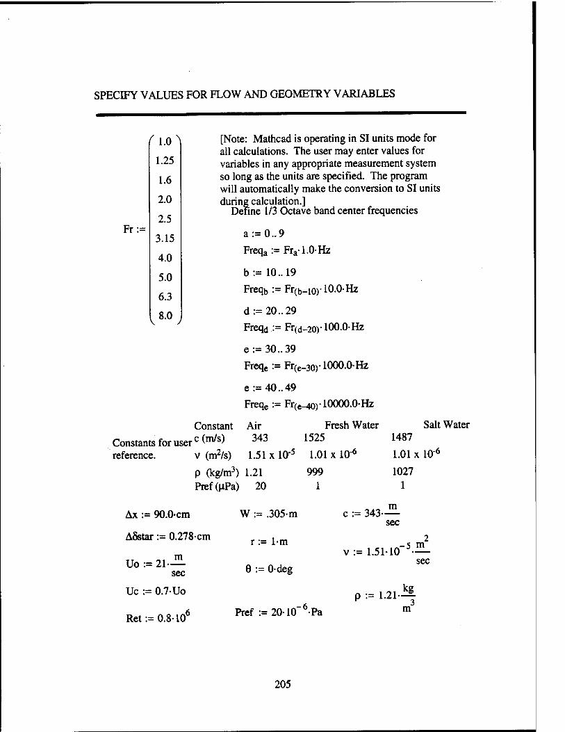
SPECIFY VALUES FOR FLOW AND GEOMETRY VARIABLES
Fr:=
r l.o ^ 1.25
1.6
2.0
2.5
3.15
4.0
5.0
6.3
8.0
[Note: Mathcad is operating in SI units mode for all calculations. The user may enter values for variables in any appropriate measurement system so long as the units are specified. The program will automatically make the conversion to SI units during calculation.]
Define 1/3 Octave band center frequencies
Constant Air
Constants for user c W*) 343
reference. v (m2/s) 1.51 x 10"5
p (kg/m3) 1.21 Pref(uPa) 20
a:=0..9
Freqa:=Fra1.0Hz
b:= 10.. 19
Freqb:=Fr(b_10)10.0-Hz
d:=20..29
Freqd .:= Fr(d_2oy 100.0- Hz
e:=30..39
Freqe := Fr(e_30)-1000.0-Hz
e:=40..49
Freqe := Fr(e_40)-10000.0-Hz
Fresh Water 1525
1.01 x 10"6
999 1
Salt Water 1487
1.01 x 10"6
1027 1
Ax := 90.0cm
A&tar := 0.278-cm
Uo := 21-^- sec
Uc := 0.7-Uo
Ret:=0.8106
W := .305m
r := 1-m
0 := 0-deg
Pref :=2010"6Pa
c := 343-^- sec
v := 1.51-10-5-^- sec
p := 1.21 kg
m
205

POWER SPECTRAL DENSITY
This section will calculate some factors which will be used in the leading terms for the final spectrum calculation.
Ret Xo := v calculated transition point
Uo F
Rexo(Xo) := Uo transition point Reynolds number v
a(Xo) := 0.0288-p-Uo2Rexo(Xo) 5
-1 ( -3\ fluctuating wall shear stress vl-11.53-Rexo(Xo)10
y
This section will define the intermittency function, y(Z), and the turbulent spot burst rate, N(Z), where Z = T}x/Ax. TO lessen computational burden later, the integrations will use another function B(Z) = N(Z)(Ax/Uo). Obviously, this just removes the factor (Uo/Ax) from the definition of N(Z) but this factor is common to both models of interest and is accounted for in the overall equation..
INTERMITTENCY FACTOR
This is the time-averaged value of the indicator function and represents the percentage of time that the flow is in a turbulent state. Either of two models for this factor can be chosen by the user for the computation of the spectrum. The empirical relation from Farabee, et al. (1974) was used in Lauchle (1980).
yFarabee(Z) := 1 - exp(-4.185-Z2) Empirical relations from Farabee, et al. (1974).
yJL(Z) := 1 - expL~(l + 3.4-Z)-Z J Empirical relations from Josserand and Lauchle (1986) which was based on the work of Gedney (1979) asessing both a Dirac line source hypothesis and a constant source hypothesis for intermitency.
**CHOOSE INTERMITTENCY FACTOR: y (Z) := YFarabee(Z)
206
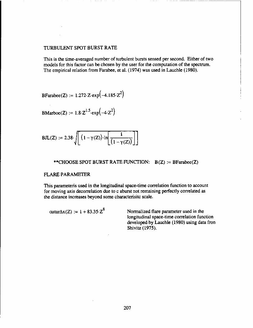
TURBULENT SPOT BURST RATE
This is the time-averaged number of turbulent bursts sensed per second. Either of two models for this factor can be chosen by the user for the computation of the spectrum. The empirical relation from Farabee, et al. (1974) was used in Lauchle (1980).
BFarabee(Z) := 1.272Zexp(-4.185-Z2)
1.5 BMarboe(Z) := 1.8-Z ' exp .(-4Z2)
BJL(Z) := 2.38- (l-Y(Z))-ln ,(l-Y(Z))J„
**CHOOSE SPOT BURST RATE FUNCTION: B (Z) := BFarabee(Z)
FLARE PARAMETER
This parameteris used in the longitudinal space-time correlation function to account for moving axis decorrelation due to c aburst not remaining perfectly correlated as the distance increases beyond some characterisitc scale.
astarAx(Z) := 1 + 83.35-Z 8 Normalized flare parameter used in the longitudinal space-time correlation function developed by Lauchle (1980) using data fron Shivitz (1975).
207
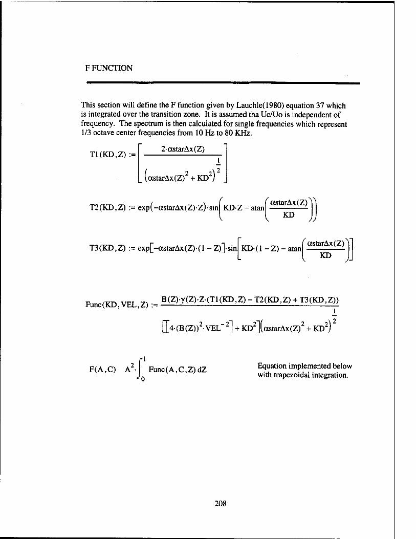
F FUNCTION
This section will define the F function given by Lauchle(1980) equation 37 which is integrated over the transition zone. It is assumed tha Uc/Uo is independent of frequency. The spectrum is then calculated for single frequencies which represent 1/3 octave center frequencies from 10 Hz to 80 KHz.
T1(KD,Z) := 2-astarAx(Z)
^astarAx(Z)' + KD2)
T2(KD,Z) := exp(-astarAx(Z)-z)-sin ( KDZ-atan
V
astarAx(Z)Y\
V KD .
T3(KD,Z) := exp[-ctstarAx(Z)-(l -Z)]-sin r^T>/, r,s (ccstarAx(Z) KD-(l-Z)-atan - KD
Func(KD,VFX,Z) := B(Z)-Y(Z)-Z-(T1(KD,Z)-T2(KD,Z) + T3(KD,Z))
[[4- (B(Z))2-VEL 2] + KD2](cestarAx(Z)2 + KD2)
F(A,C) A- Func(A,C,Z)dZ Equation implemented below with trapezoidal integration.
208

SPECTRAL CALCULATIONS
Define frequency range
fmax := 5000-Hz
points := 1000
nn := 1.. points + 1
ORIGIN := 1
KL:=1000 k:=l..KL fk := fmax-10 KL
—l
^nn •- nn- 1
points
intk,nn := Func Ax Uc ^
v Uc Uo
dZ:= points
FF •= P\ (intk,nn+l+intk,nn) ^
nn = 1
Definition of function representing power spectral density:
Fk:=|2-7t-fk~j FFk
Gk:= [w-(o(Xo))2-(cos(e))2-Uo-(Ax)2]-Fk
<•> 2 2 2 2-r -n -c
Calculation of power spectral density:
SPECGk := 10-log Gk
(Pref)" Hz
209
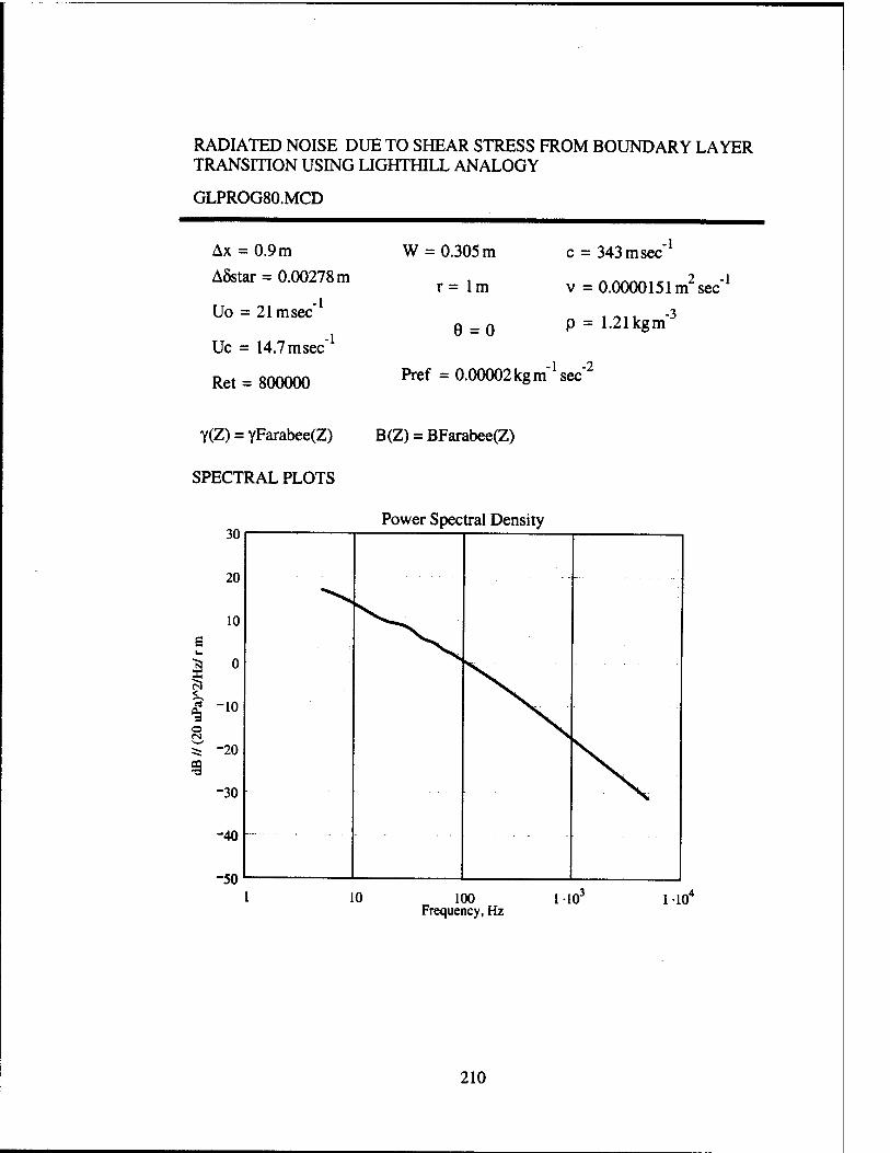
RADIATED NOISE DUE TO SHEAR STRESS FROM BOUNDARY LAYER TRANSITION USING LIGHTHILL ANALOGY
GLPROG80.MCD
Ax = 0.9 m ASstar = 0.00278 m
-l Uo = 21msec
Uc = 14.7 msec
Ret = 800000
■l
c = 343 msec W = 0.305 m
r = lm
9 = 0 P = 121kgm
Pref = 0.00002 kg m"1 sec"2
l
v = 0.0000151m2 sec"1
-3
Y(Z) = yFarabee(Z) B(Z) = BFarabee(Z)
SPECTRAL PLOTS
Power Spectral Density
100 Frequency, Hz
110J 110'
210

REFERENCES
Farabee, T. M., Casarella, M. J., and DeMetz, F. C, 1974, "Source Distribution of Turbulent Bursts During Natural Transition," David W. Taylor Naval Ship Research and Development Center Report SAD-89E-1942, August 1974.
Gedney, C. J., 1979, "Wall Pressure Fluctuations During Transition on a Flat Plate," Massachusetts Institute of Technology Report 84618-1.
Josserand, M. A. and Lauchle, G. C, 1986, "Wavevector-Frequency Spectrum of Transition Zone Wall Pressure Fluctuations," ARL Penn State Technical Report TR 86-008, December 1986.
Shivitz, W. F., 1975, "An Experimental Investigation of Artificially Induced Transition to Turbulence on a Body of Revolution," M.S. Thesis, The Pennsylvania State University.
MODIFICATION HISTORY
Original 7 May 1998 Conversion of elements of GLPROG VAX program Mod 1 14 May 1998 Addition of choices for intermittency and burst rate
functions Mod 2 4 July 2000 Substitution of trapezoidal integration.
Spectrunr ' := f-sec
Spectrum^2' := SPECG
B Zi.VWQAFFF2t.TXT
Spectrum
211
A.2 Fluctuating Boundary Layer Displacement Thickness Using a Liepmann Analogy - Theoretical Space-Time Correlation Function
Mathcad file: GLPROG81.MCD
212
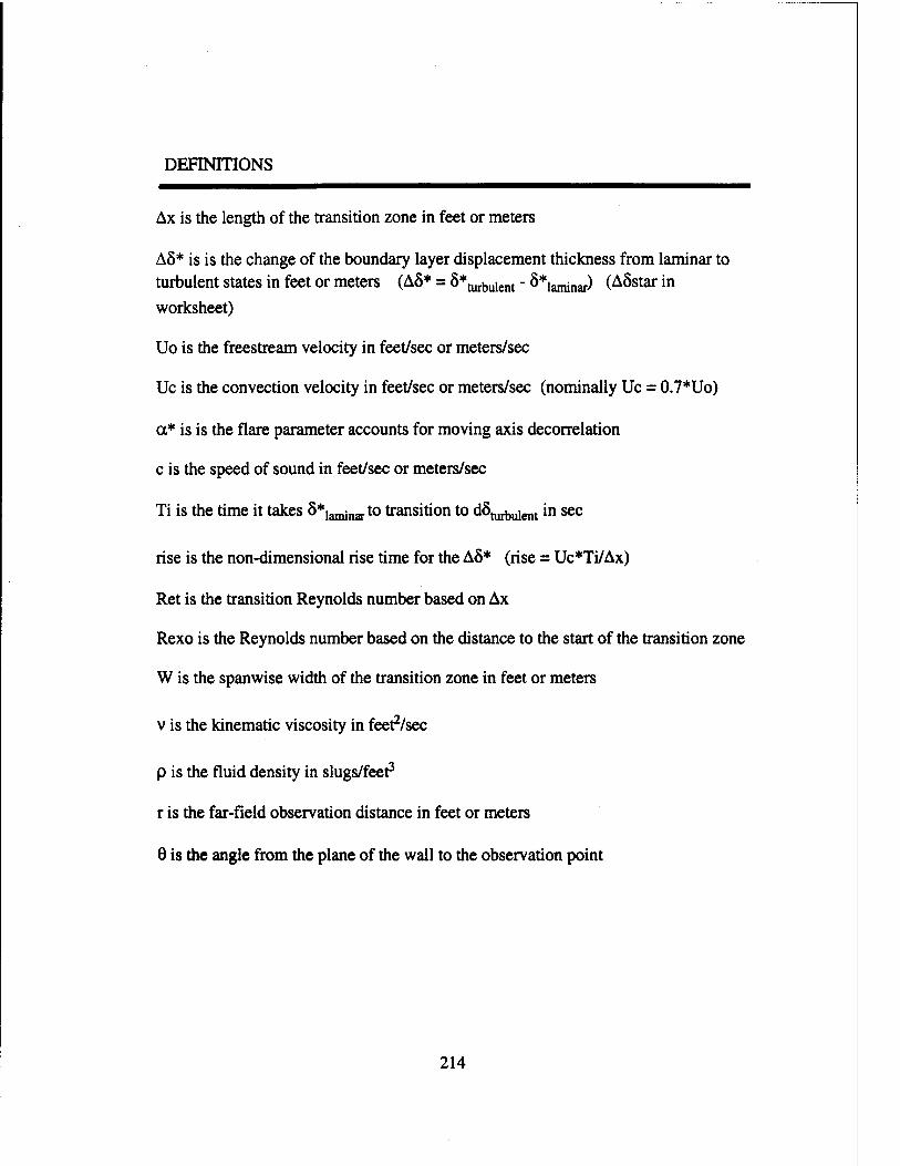
DEFINITIONS
Ax is the length of the transition zone in feet or meters
AS* is is the change of the boundary layer displacement thickness from laminar to turbulent states in feet or meters (AS* = 8*turbulent - 5*laminar) (ASstar in
worksheet)
Uo is the freestream velocity in feet/sec or meters/sec
Uc is the convection velocity in feet/sec or meters/sec (nominally Uc = 0.7*Uo)
a* is is the flare parameter accounts for moving axis decorrelation
c is the speed of sound in feet/sec or meters/sec
Ti is the time it takes 8*laminarto transition to dS^,,^ in sec
rise is the non-dimensional rise time for the AS* (rise = Uc*Ti/Ax)
Ret is the transition Reynolds number based on Ax
Rexo is the Reynolds number based on the distance to the start of the transition zone
W is the spanwise width of the transition zone in feet or meters
v is the kinematic viscosity in feeAsec
p is the fluid density in slugs/feet3
r is the far-field observation distance in feet or meters
0 is the angle from the plane of the wall to the observation point
214

SPECIFY VALUES FOR FLOW AND GEOMETRY VARIABLES
fun [Note: Mathcad is operating in SI units mode for
1.25 all calculations. The user may enter values for variables in any appropriate measurement system
1.6 so long as the units are specified. The program will automatically make the conversion to SI units
2.0 during calculation.] Define 1/3 Octave band center frequencies 2.5
Fr:= 3.15 a:=0..9
4.0 Freqa:=Fra1.0-Hz
5.0 b := 10.. 19
6.3 Freqb:=Fr(b_10)-10.0-Hz
.8.0 d:=20..29
Freqd := Fr(d_20)-100.0-Hz
e:=30..39
Freqc := Fr(e-30)-1000.0-Hz
f :=40..49
Freqf := Fr(f_40)-10000.0-Hz
Constant- Constant Air Fresh Water Salt Water s for user c (m/s) 343 1525 1487 reference. v (m2/s) 1.51 x 10'5 1.01 x 10"6 1.01 x 10'6
p (kg/m3) 1.21 999 1027 Pref(nPa) 20 1 1
Ax := 2.82-cm Ti := 0.45-sec ,,„- m c := 1525 ASstar := 0.021cm nie sec
rise := 0.15 2
m v:=1.01-10-6-^- Uo := 21.0-— W := .305-m sec
sec
Uc := 0.7-Uo r := 1.0-m Pref := 110 Pa
Ret:= 1.5106 p := 999-^- 3 m
215
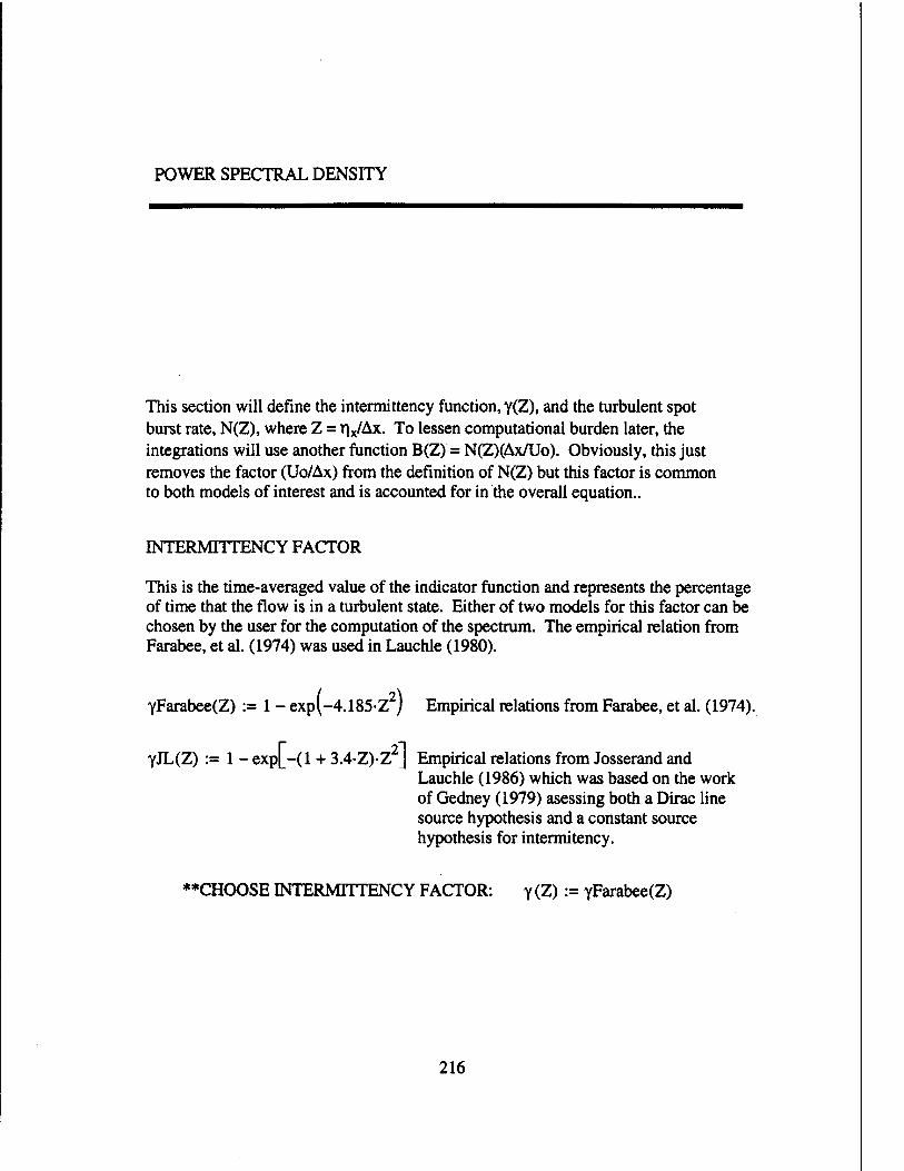
POWER SPECTRAL DENSITY
This section will define the intermittency function, y(Z), and the turbulent spot burst rate, N(Z), where Z = r|x/Ax. To lessen computational burden later, the integrations will use another function B(Z) = N(Z)(Ax/Uo). Obviously, this just removes the factor (Uo/Ax) from the definition of N(Z) but this factor is common to both models of interest and is accounted for in the overall equation..
DSfTERMnTENCY FACTOR
This is the time-averaged value of the indicator function and represents the percentage of time that the flow is in a turbulent state. Either of two models for this factor can be chosen by the user for the computation of the spectrum. The empirical relation from Farabee, et al. (1974) was used in Lauchle (1980).
YFarabee(Z) := 1 - exp(-4.185-Z j Empirical relations from Farabee, et al. (1974).
yJL(Z) := 1 - exp[-(l + 3.4-Z)-Z J Empirical relations from Josserand and Lauchle (1986) which was based on the work of Gedney (1979) asessing both a Dirac line source hypothesis and a constant source hypothesis for intermitency.
**CHOOSE INTERMITTENCY FACTOR: y (Z) := YFarabee(Z)
216
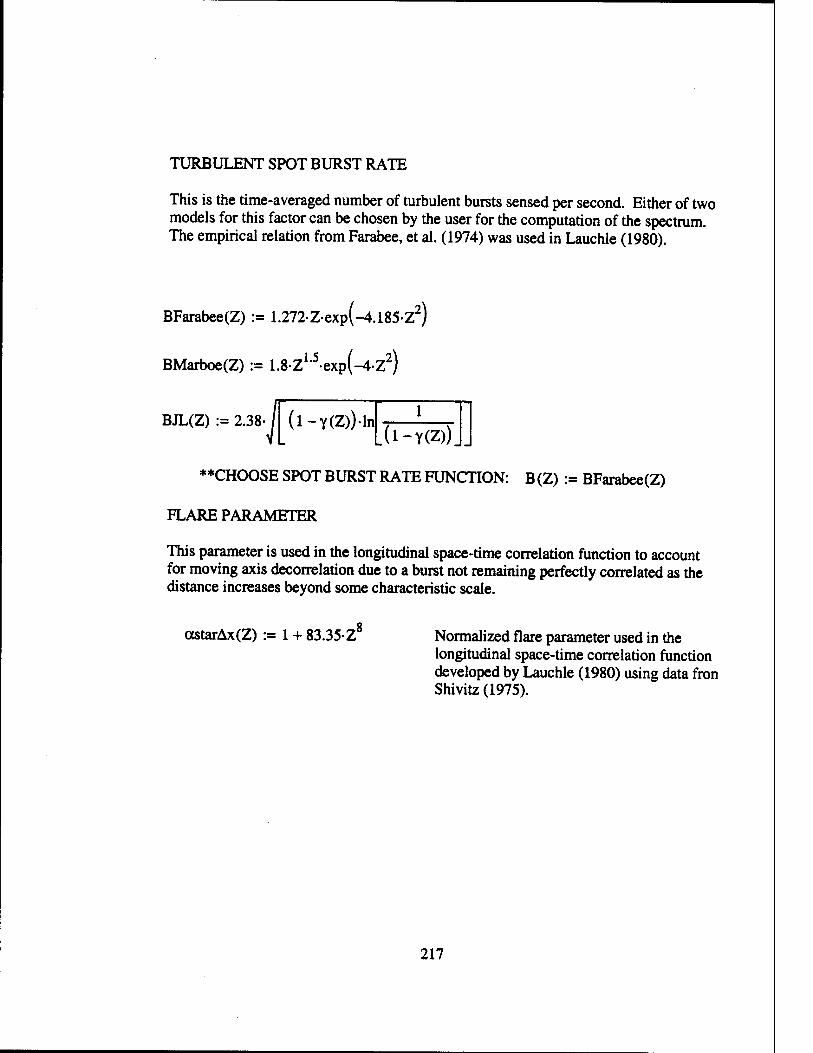
TURBULENT SPOT BURST RATE
This is the time-averaged number of turbulent bursts sensed per second. Either of two models for this factor can be chosen by the user for the computation of the spectrum. The empirical relation from Farabee, et al. (1974) was used in Lauchle (1980).
BFarabee(Z) := 1.272-Z-exp(-4.185-Z2)
BMarboe(Z) := 1.8-ZL5exp(-4-Z2)
BJL(Z) := 2.38- (l-Y(Z))-ln _(l-Y(Z))J_
**CHOOSE SPOT BURST RATE FUNCTION: B (Z) := BFarabee(Z)
FLARE PARAMETER
This parameter is used in the longitudinal space-time correlation function to account for moving axis decorrelation due to a burst not remaining perfectly correlated as the distance increases beyond some characteristic scale.
astarAx(Z) := 1 + 83.35-Z Normalized flare parameter used in the longitudinal space-time correlation function developed by Lauchle (1980) using data fron Shivitz (1975).
217
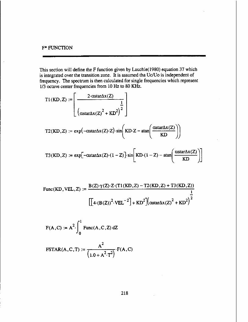
F* FUNCTION
This section will define the F function given by Lauchle(1980) equation 37 which is integrated over the transition zone. It is assumed tha Uc/Uo is independent of frequency. The spectrum is then calculated for single frequencies which represent 1/3 octave center frequencies from 10 Hz to 80 KHz.
T1(KD,Z) := 2-astarAx(Z)
tastarAx(Z)' + KD2)
T2(KD,Z) := exp(-astarAx(Z)-Z)-sin ( KDZ - atan
V
astarAx(Z)Y m JJ T3(KD,Z) := exp[-ccstarAx(Z)-(l -Z)]-sin KD-(l-Z)-atan
astarAx(Z) KD M
Func(KD,VEL,Z) := B(Z)-Y(Z)-Z-(T1(KD,Z)-T2(KD,Z)+ T3(KD,Z))
[]>(B(Z))2-VEL 2] + KD2](ocstarAx(Z)2 + KD2)
/*!
F(A,C) := A' Func(A,C,Z)dZ
FSTAR(A,C,T) := (l.0 + A2-T2)
F(A,C)
218
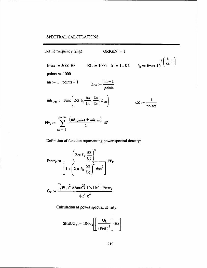
SPECTRAL CALCULATIONS
Define frequency range ORIGIN := 1
•PL- fmax := 5000-Hz KL := 1000 k := 1.. KL fk := fmax-10 ^
points := 1000
nn := 1.. points + 1 ^nn •-
nn- 1
points
intk,nn := Func f. . Ax Uc „
2-71-fir , jZnn Uc Uo dZ:=
points
points /. . ,. „ \ FF = V lintk,nn+l+mtk)nnJ ^
nn = 1
Definition of function representing power spectral density:
Fstark := ^
2-rc-fk
( 1 +
~ * Ax 2-n-fv—
Uc
\2 TFFk
. 2 rise
Gk:= [(W-p2- ASstar2) -Uo-Uc2]-Fstaik
8-rV
Calculation of power spectral density:
SPECGk := 10- log Gk
(Pref)' Hz
219
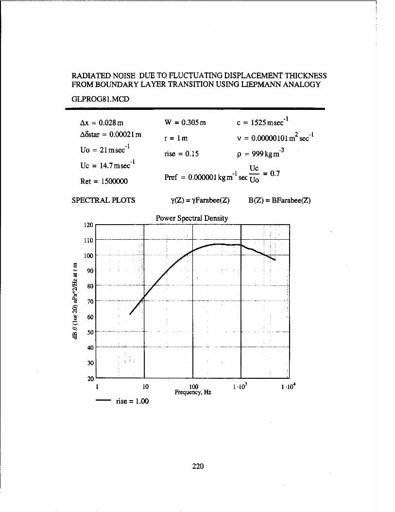
RADIATED NOISE DUE TO FLUCTUATING DISPLACEMENT THICKNESS FROM BOUNDARY LAYER TRANSITION USING LIEPMANN ANALOGY
GLPROG81.MCD
Ax = 0.028 m ASstar = 0.00021m
-l Uo = 21msec
Uc = 14.7 msec
Ret = 1500000
-l
W = 0.305 m
r = lm
rise = 0.15
c = 1525 msec l
v = 0.00000101m2 sec"1
p = 999 kg m"
Uc Pref = 0.000001 kg m'1 sec Uo ~ °'7
SPECTRAL PLOTS
120
110
100
E £ 90
S 80 <
^ 70
60 o
50
40
30
20 1
Y(Z) = YFarabee(Z)
Power Spectral Density
B(Z) = BFarabee(Z)
10
rise = 1.00
100 Frequency, Hz
110° 110"
220
REFERENCES
Farabee, T. M, Casarella, M. JM and DeMetz, F. C, 1974, "Source Distribution of Turbulent Bursts During Natural Transition," David W. Taylor Naval Ship Research and Development Center Report SAD-89E-1942, August 1974.
Gedney, C. J., 1979, "Wall Pressure Fluctuations During Transition on a Flat Plate," Massachusetts Institute of Technology Report 84618-1.
Josserand, M. A. and Lauchle, G. C, 1986, "Wavevector-Frequency Spectrum of Transition Zone Wall Pressure Fluctuations," ARL Penn State Technical Report TR 86-008, December 1986.
Lauchle, G. C, 1980, 'On the radiated noise due to boundary-layer transition,'/. Acous. Soc. ofAmer., 67, pp.158-168.
Shivitz, W. F., 1975, "An Experimental Investigation of Artificially Induced Transition to Turbulence on a Body of Revolution," M.S. Thesis, The Pennsylvania State University.
MODIFICATION HISTORY
Original 7 June 1998 Conversion of elements of GLPROG VAX program Mod 1 7 June 1998 Addition of choices for intermittency and burst rate
functions Mod 2 4 July 2000 Substituted trapezoidal integration
Spectnmr ' := f-sec
Spectrum^ := SPECG
fl Z1\81WATERFF21.TXT
Spectrum
221
A.3 Fluctuating Boundary Layer Displacement Thickness Using a Liepmann
Analogy - Theoretical Space-Time Correlation Function with Krane Dipole
Source Model
Mathcad file: KMTRANSOO.MCD
222

RADIATED NOISE DUE TO FLUCTUATING DISPLACEMENT THICKNESS FROM BOUNDARY LAYER TRANSITION USING A LIEPMANN ANALOGY WITH KRANE DIPOLE MODEL
[KMTRANS00.MCD, Mathcad 2000 Professional]
This program is the implementation of a boundary layer transition noise model described in: Lauchle, G. C, 1981, 'Transition noise - The role of fluctuating displacement thickness,'/. Acous. Soc. ofAmer., 69, pp.665-671.
However, the source term has benn modified to replace the monopole with a dipole derived from the measurements cited in: Krane, M. H., 1992, "Estimation of the Direct Acoustic Radiation from Turbulent Spots, Using Boundary Layer Velocity Measurements," Ph.D. Thesis in Aerospace Engineering, The Pennsylvania State University.
ASSUMPTIONS - builds on fluctuating shear stress model [Lauchle 1981] - zero pressure gradient flow and natural transition flow structures, i.e. no separation). - flow is over an infinite, planar, rigid surface - based on very low Mach number - use only dipole components due to fluctuating displacement thickness - flow is statistically homogeneous in spanwise direction, X3, non-homogeneous in streamwise direction, xi, stationary but Poisson distributed in time so we can use a classical correlation function for a random sequence of bursts, exp(-2N|t|) - neglect quadrupoles and octupoles due to fluctuating Reynolds stresses due to lower radiation efficiencies - however, their amplitudes relative to shear stresses may overcome this lower efficiency. - the space-time correlation function for the indicator function <IT>is direction separable - the lateral term integration derived from this separation is equal to 21^(11!) = 2(1.5 Tli tan a) which is about r\xIA for a=9.6 degrees (angle of spreading for turbulent spot) - Uc/Uo is independent of frequency - the normalized rise time is described as a function of r\ j/Ax
223
DEFINITIONS
Ax is the length of the transition zone in feet or meters
AS* is is the change of the boundary layer displacement thickness from laminar to turbulent states in feet or meters (AS* = 5*^,^ - 5*laminar) (ASstar in
worksheet)
Uo is the freestream velocity in feet/sec or meters/sec
Uc is the convection velocity in feet/sec or meters/sec (nominally Uc = 0.7*Uo)
a* is is the flare parameter accounts for moving axis decorrelation
c is the speed of sound in feet/sec or meters/sec
Ti is the time it takes 8*laminarto transition to clStlutHltem in sec
rise is the non-dimensional rise time for the AS* (rise = Uc*Ti/Ax)
Ret is the transition Reynolds number based on Ax
Rexo is the Reynolds number based on the distance to the start of the transition zone
W is the spanwise width of the transition zone in feet or meters
v is the kinematic viscosity in fee^/sec
p is the fluid density in slugs/feet3
r is the far-field observation distance in feet or meters
9 is the angle from the plane of the wall to the observation point
224
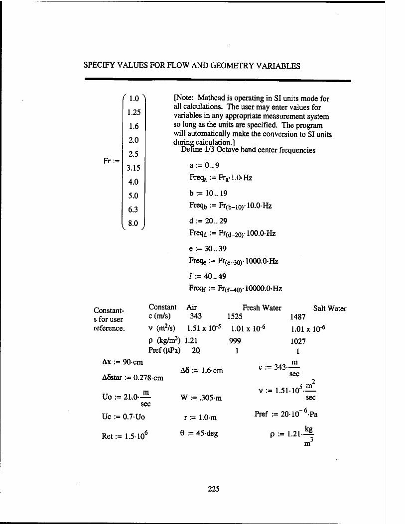
SPECIFY VALUES FOR FLOW AND GEOMETRY VARIABLES
(l.(P [Note: Mathcad is operating in SI units mode for
1.25 all calculations. The user may enter values for variables in any appropriate measurement system
1.6 so long as the units are specified. The program will automatically make the conversion to SI units
2.0 during calculation.] Define 1/3 Octave band center fn 2.5 jquencies
Fr:= 3.15 a:=0..9
4.0 Freqa:=Fra-1.0-Hz
5.0 b:= 10.. 19
6.3 Freqb:=Fr(b_10)10.0-Hz
8.0 d:=20..29 < J
Freqd:=Fr(d_20)-100.0-Hz
e:=30..39
Freqe := Fr(e_30)-1000.0-Hz
f :=40..49
Freqf := Fr(f^o)-10000.0-Hz
Constant- Constant Air Fresh Water Salt Water s for user c (m/s) 343 1525 1487 reference. v (m2/s) 1.51 x 10"5 1.01 x lO'6 1.01 x 10"6
p (kg/m3) 1.21 999 1027 Pref(uPa) 20 1 1
Ax := 90cm m A5 := 1.6-cm c := 343 •
A5star := 0.2' 78-cm sec
m v := 1.51-105 — Uo := 21.0- W := .305m sec
sec
Uc := 0.7-Uo r:=1.0-m Pref := 20-10" °-Pa
Ret:= 1.5-10 6 9 := 45-deg p := 1.21-M 3 m
225
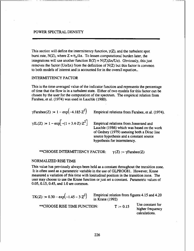
POWER SPECTRAL DENSITY
This section will define the intermittency function, Y(Z), and the turbulent spot burst rate, N(Z), where Z =r|x/Ax. To lessen computational burden later, the integrations will use another function B(Z) = N(Z)(Ax/Uo). Obviously, this just removes the factor (Uo/Ax) from the definition of N(Z) but this factor is common to both models of interest and is accounted for in the overall equation..
INTERMnTENC Y FACTOR
This is the time-averaged value of the indicator function and represents the percentage of time that the flow is in a turbulent state. Either of two models for this factor can be chosen by the user for the computation of the spectrum. The empirical relation from Farabee, et al. (1974) was used in Lauchle (1980).
yFarabee(Z) := 1 -exp(-4.185-Z2)
yJL(Z) := 1 - exp[-(l + 3.4-Z)-Z2]
Empirical relations from Farabee, et al. (1974).
Empirical relations from Josserand and Lauchle (1986) which was based on the work of Gedney (1979) asessing both a Dirac line source hypothesis and a constant source hypothesis for intermitency.
**CHOOSE INTERMnTENCY FACTOR: y(Z) := yFarabee(Z)
NORMALIZED RISE TIME
This value has previously always been held as a constant throughout the transition zone. It is often used as a parametric variable in the use of GLPROG81. However, Krane measured a variation of this time with lonitudinal position in the transition zone. The user may choose to use the Krane function or just set a constant. Parametric values of 0.05,0.15,0.45, and 1.0 are common.
Tvf7\ . nin ~ ( \ A< i^A Empirical relation from figures 4.15 and 4.20 TK(Z) .= 0.30 - expl-1.45 - 3Z ) ^ ^ (m2)
**CHOOSE RISE TIME FUNCTION: T := 0.15 Use constant for higher frequency calculations.
226
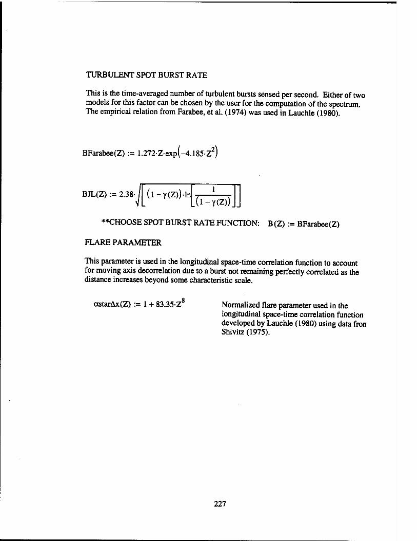
TURBULENT SPOT BURST RATE
This is the time-averaged number of turbulent bursts sensed per second. Either of two models for this factor can be chosen by the user for the computation of the spectrum. The empirical relation from Farabee, et al. (1974) was used in Lauchle (1980).
BFarabee(Z) := 1.272-Z-exp(-4.185-Z2)
BJL(Z) := 2.38- (l-Y(Z))-ln _(l-Y(Z))J_
**CHOOSE SPOT BURST RATE FUNCTION: B (Z) := BFarabee(Z)
FLARE PARAMETER
This parameter is used in the longitudinal space-time correlation function to account for moving axis decorrelation due to a burst not remaining perfectly correlated as the distance increases beyond some characteristic scale.
ccstarAx(Z) := 1 + 83.35-Z 8 Normalized flare parameter used in the longitudinal space-time correlation function developed by Lauchle (1980) using data fron Shivitz (1975).
227
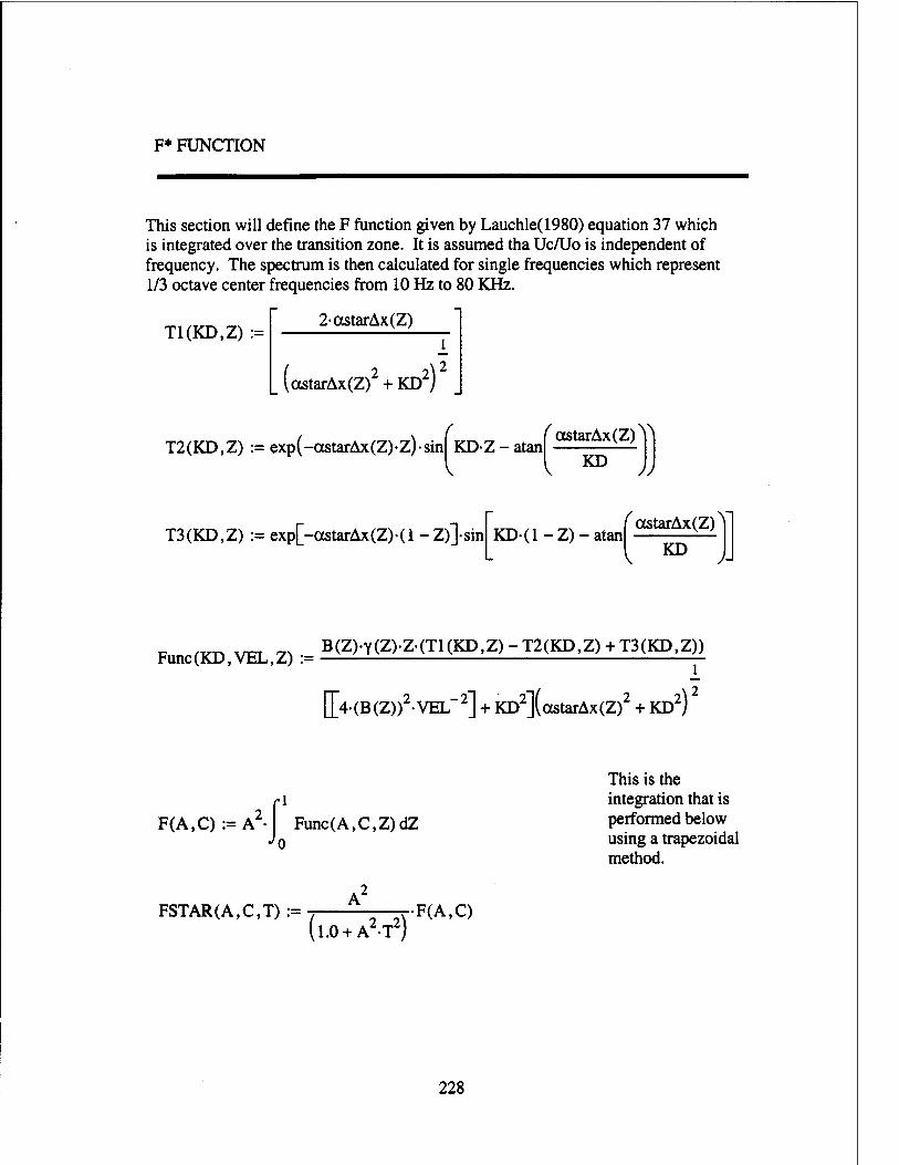
F* FUNCTION
This section will define the F function given by Lauchle(1980) equation 37 which is integrated over the transition zone. It is assumed tha Uc/Uo is independent of frequency. The spectrum is then calculated for single frequencies which represent 1/3 octave center frequencies from 10 Hz to 80 KHz.
T1(KD,Z) := 2astarAx(Z)
kctstarAx(Z)2 + KD2)
T2(KD,Z) := exp(-ccstarAx(Z)-z)-sin / KDZ - atan
V.
ctstarAx(Z) KD
\\
JJ
T3(KD,Z) := exp[-astarAx(Z)-(l -Z)]-sin KD-(l-Z)-atan (
\
ccstarAx(Z) KD yj
Func(KD,VFX,Z) := B(Z)-Y(Z)-Z-(T1(KD,Z) - T2(KD,Z) + T3(KD,Z))
0>(B(Z))2-VEL 2] + KD2](ctstarAx(Z)2 + KD2)
rl F(A,C) := A' Func(A,C,Z)dZ
This is the integration that is performed below using a trapezoidal method.
FSTAR(A,C,T) := (I.O+A¥)
F(A,C)
228
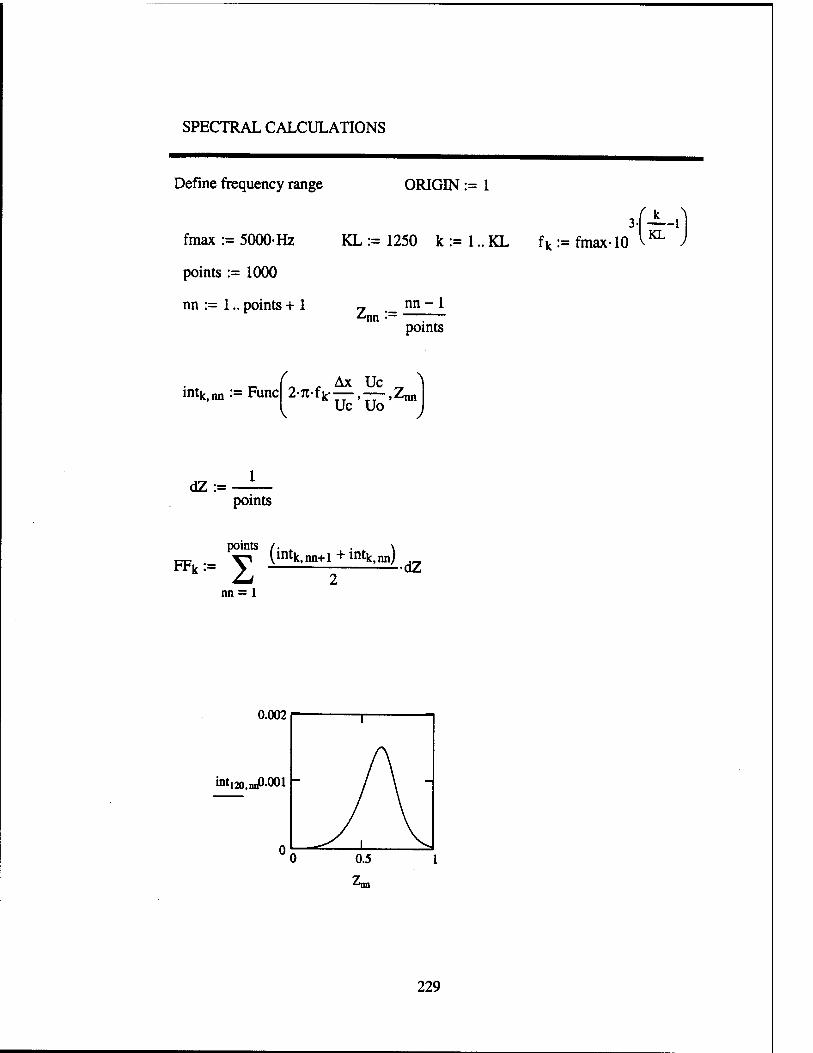
SPECTRAL CALCULATIONS
Define frequency range
fmax := 5000-Hz
points := 1000
nn := 1.. points + 1
ORIGIN := 1
KL := 1250 k := 1.. KL fk := fmax-10
^nn •- -•nn nn- 1
points
^
/ intk,nn := Func
,.f Ax Uc
Uc Uo
\
J
dZ:= points
points /. . . \ FF = V ^mtk'nn+1+intk'nn) j2
nn = 1
0.002
«nti20,mP001 -
229
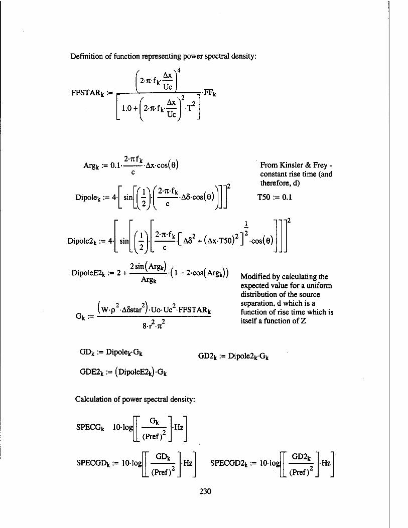
Definition of function representing power spectral density:
FFSTARk := F
2-7t-fk Uc
( 1.0 + 2-7t-fk-
Uc
= FFk
•T2
2-7tfk / \ Argk := 0.1 Ax-cos(0)
Dipolek := 4 sin (\ Aocos^GJ
M
-a
Dipole2k := 4' sm f\_
From Kinsler & Frey - constant rise time (and therefore, d)
T50 := 0.1
-1-112
^-^•[A52 + (AX-T50)
2] -cos(e)
2sin(Argk) , . .. DipoleE2k := 2 + —— (1 - 2-cos(Argk)) Modified by calculating ±e
Gk:=
Argk
ASstar2) Uo-Uc"FFSTARk (wp2A5star2)-Uo-TT 2
o-r -7t
expected value for a uniform distribution of the source separation, d which is a function of rise time which is itself a function of Z
GDk := DipolekGk
GDE2k := (DipoleE2k)-Gk
GD2k := Dipole2kGk
Calculation of power spectral density:
SPECGk 10-log Gk
(Pref) Hz
SPECGEhc := 10-log (Pref)2
Hz SPECGD2k := 10-log GD2k
(Pref)2 Hz
230
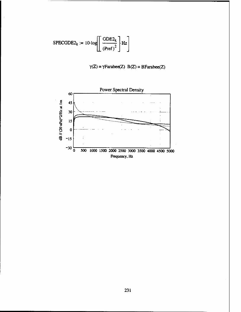
SPECGDE2k := 10- log GDE2k
(Pref)2 Hz
Y(Z) = YFarabee(Z) B(Z) = BFarabee(Z)
Power Spectral Density
0 500 1000 1500 2000 2500 3000 3500 4000 4500 5000
Frequency, Hz
231
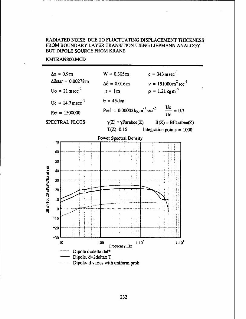
RADIATED NOISE DUE TO FLUCTUATING DISPLACEMENT THICKNESS FROM BOUNDARY LAYER TRANSITION USING HERMANN ANALOGY BUT DIPOLE SOURCE FROM KRANE
KMTRANS00.MCD
Ax = 0.9 m ASstar = 0.00278 m
-l Uo = 21msec
-l Uc = 14.7 msec
Ret = 1500000
SPECTRAL PLOTS
70
60
50
E 5 40
5 30
20
10
0
-10
-20
<
o
-30 10
-1
v = 151000 m2 sec"1
-3
W = 0.305 m c = 343 msec
AS = 0.016m
r = Im p = 1.21 kgm
9 = 45deg
Pref = 0.00002 kgm"1 sec"2 — = 0.7 Uo
Y(Z) = YFarabee(Z) B(Z) = BFarabee(Z)
T(Z)=0.15 Integration points = 1000
Power Spectral Density
•**'" r '<
100 1 103
Frequency, Hz
Dipole d=delta del* Dipole, d=2deltax T Dipole- d varies with uniform prob
110*
232
REFERENCES
Farabee, T. M., Casarella, M. J., and DeMetz, F. C, 1974, "Source Distribution of Turbulent Bursts During Natural Transition," David W. Taylor Naval Ship Research and Development Center Report SAD-89E-1942, August 1974.
Gedney, C. J., 1979, "Wall Pressure Fluctuations During Transition on a Flat Plate," Massachusetts Institute of Technology Report 84618-1.
Josserand, M. A. and Lauchle, G. C, 1986, "Wavevector-Frequency Spectrum of Transition Zone Wall Pressure Fluctuations," ARL Penn State Technical Report TR 86-008, December 1986.
Lauchle, G. C, 1980, 'On the radiated noise due to boundary-layer transition,'/. Acous. Soc. ofAmer., 67, pp.158-168.
Pierce, A. D., 1981, Acoustics - An Introduction to its Physical Principles and Applications, McGraw-Hill, New York.
Shivitz, W. F., 1975, "An Experimental Investigation of Artificially Induced Transition to Turbulence on a Body of Revolution," M.S. Thesis, The Pennsylvania State University.
MODIFICATION HISTORY
Original 8 June 2000 Conversion of GLPROG81 to replace monopole with dipole source and put in normailized rise
time as a function of Z
Mod 1 14 June 2000 Upgraded dipole source term to eliminate kd«l low frequency assumption.
Spectnmv ' := f-sec
Spectrum^ := SPECGD2
Spectrum'3' := SPECGDE2 y
MM!RANSWFF2ie.T](T
Spectrum
233
A.4 Fluctuating Boundary Layer Displacement Thickness Using a Liepmann Analogy - Empirical Space-Time Correlation Function
Mathcad file: JLTRANS99.MCD
234

BOUNDARY LAYER TRANSITION ZONE SOUND RADIATION USING JOSSERAND'S EMPIRICAL SPACE-TIME CORRELATION
[JLTRANS99.MCD. Mathcad 2000 Professional]
This program is the implementation of a boundary layer transition noise model described in: Lauchle, G. C, 1981. Transition noise - The role of fluctuating displacement
thickness,'/ Aeons. Soc. ofAmer.. 69, pp.665-67l.
Josserand, M. A. and Lauchle. G. C, 1989. "Cross-Spectral Density of the Wall Pressure Fluctuations Under a Turbulent Boundary Layer," J. Sound Vib. 128. pp. 519-522.
Josserand, M. A. and Lauchle. G. C. 1990. "Modeling the Wavevector- Frequency Spectrum or Boundary Layer Wall Pressure During Transition on a Flat Plate," Trans. ASME. J. Vib. and Acoustics 112, pp. 523-534.
ASSUMPTIONS - builds on fluctuating displacemtn thickness model [Lauchle 1981] - zero pressure gradient flow and natural transition flow structures, i.e. no
separation). - flow is over an infinite, planar, rigid surface - based on very low Mach number - uses enmpitrical description for Cross correlation function developed by
Josse rand - Uc/Uo is independent of frequency
DEFINITIONS
Define transition zone length (Ax) and free-stream velocity (U)
Ax:=0.9.m U:=21 — sec
Turbulent spot convection velocity Uc := 0.8-U
Intermittancy factor, Josserand & Lauchle (1990) eqn. 11
c3:=1.0 c4:=3.4
,\2
Y(T,x):=l-exp|4c3 + c4.^.Ui
235
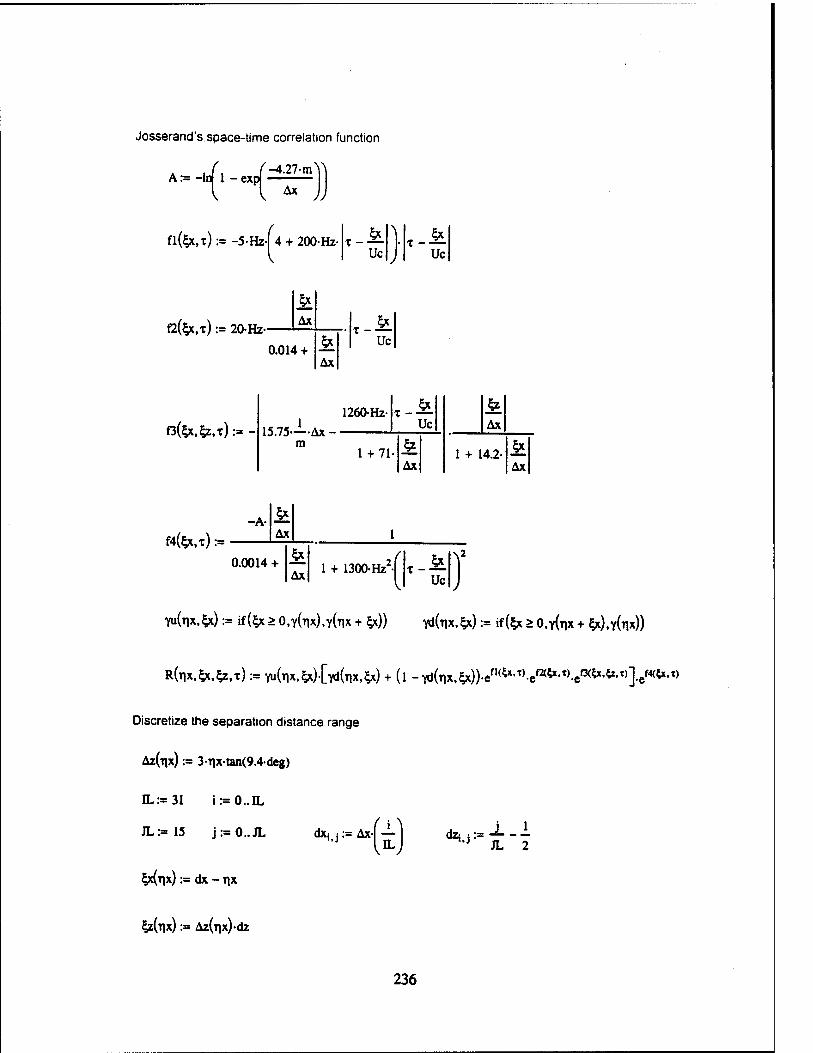
Josserand's. space-time correlation function
A:=-ln( l-exp| -4.27- m
Ax
fl(5x,T):=-5-Hz-|4 + 200-Hz- T - Uc
T -■ Uc
f2(§x,t) := 20-Hz- Ax
0.014 + Ax
T -• Uc
G(SX,SZ,T):=-
1260-Hz-
15.75—Ax - ■ m
Uc
1 + 71- Ax
Ax
1 + 14.2 Ax
f4tec,t) :=
-A- Ax
0.0014 + Ax 1 + UOO-Hz' T -
Uc
yi(r\x,Zx) := if (£x > 0,Y(TIX),Y(TIX + ^x)) yd(i]x,&) := if {& > O.YOIX + £X),Y(TIX))
R{t\x,£x,b,x) := yi(r\x,tx)-[yd{t\x,Zx) + (l -^{r\x,^)).tn^'x)-^^x).t^'^'x)].cf^^
Oiscretize the separation distance range
AZ(TIX) := 3rix-tan(9.4deg)
IL:= 31 i:=0..IL
JL:=15 j:=0..JL
§X(TIX) := dx - r\x
&(r\x) := Az(rix)dz
dx^Ax-j- dZi.j ~ JL 2
236
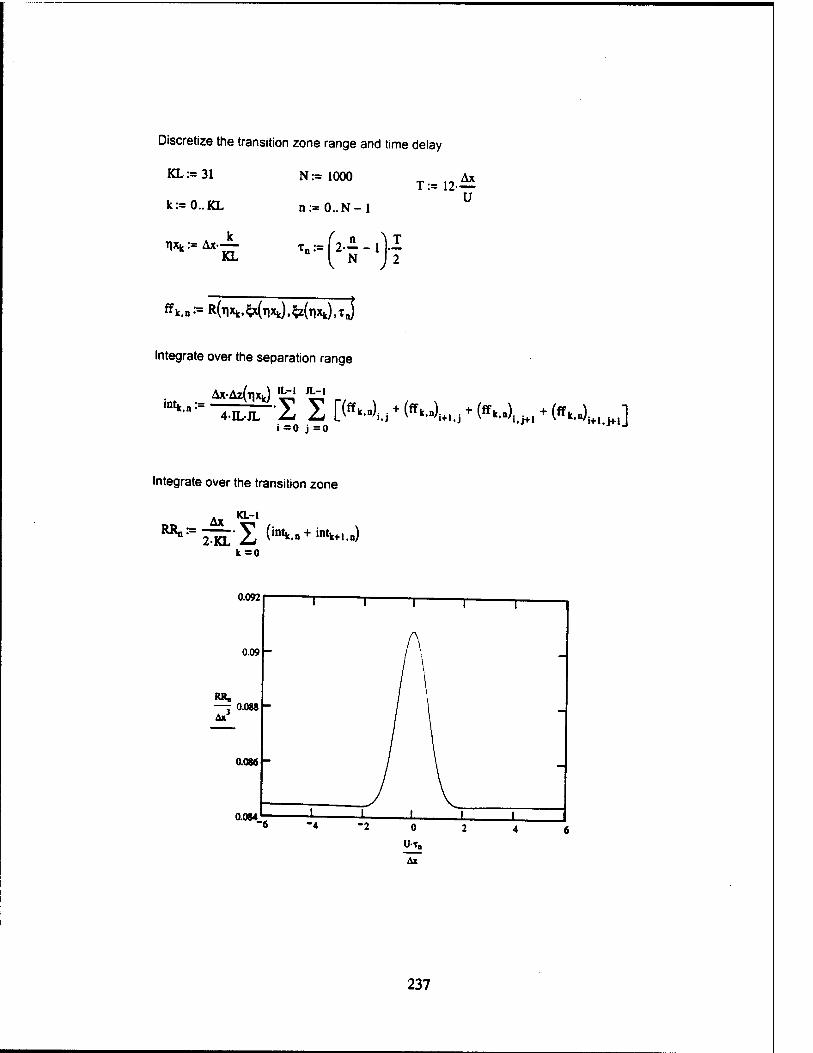
Discretize the transition zone range and time delay
KL := 31 N := 1000
k:=0..KL n:=0..N-l
T:=12-^ U
iixij := Ax KL
t„:=
ff k,n := »(TlXk.^TlxJ.^TlxJ.TJ
Integrate over the separation range
i=0 j =0 J
Integrate over the transition zone
Ax KL-t
^"IKL'X (intk.»+intk+l.n) k=0
0.092
0.09 -
0.088 -
0.086 -
0.084
237
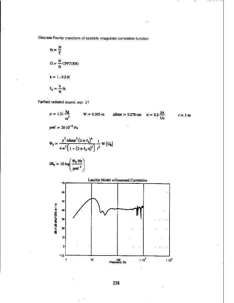
Discrete Fourier transform of spatially integrated correlation function
fs:= — T
N G:= —CFFT(RR)
fs
k:= 1..0.5-N
fk := —fs N
Farfield radiated sound, eqn. 21
kg p := 1.21- W := 0.305m m
ASstar := 0.278-cm ti := 0.2 — Uc
r:= 1-m
prcf :=2010 -Pa
4-re(l + (2-n-fk-ti)2J r2
dBk := 10-log <t>tHzN
pref2,
70
60
50 S
2 *°
| 30
s
10
0
-10
Lauchle Model w/Josserand Correlation
10 100 1 10-* Frequency, Hz 110'
238
REFERENCES
Farabee, T. M., Casarella. M. J., and DeMetz, F. C, 1974, "Source Distribution of Turbulent Bursts During Natural Transition," David W. Taylor Naval Ship Research and Development Center Report SAD-89E-1942, August
Gedney, C. J., 1979, "Wall Pressure Fluctuations During Transition on a Flat Plate," Massachusetts Institute of Technology Report 84618-1.
Josserand, M. A. and Lauchle. G. C, 1986, "Wavevector-Frequency Spectrum of Transition Zone Wall Pressure Fluctuations." ARL Penn State Technical Report TR 86-008, December 1986.
Lauchle, G. C, 1980, On the radiated noise due to boundary-layer transition ' J. Acous. Soc. of Amen, 67, pp. 158-168.
Shivitz, W. F., 1975, "An Expenmental Investigation of Artificially Induced Transition to Turbulence on a Body of Revolution," M.S. Thesis, The Pennsylvania State University.
Spectrum'1' := f-sec
Spectrum^ := dB
B ZV.ULTRANS QAF211.TXT
Spectrum
239
A.5 Noise Generated by Boundary Layer Transition on Symmetric Hydrofoils Howe Formulation
Mathcad file: MSHTRANS99.MCD
240
BOUNDARY LAYER TRANSITION NOISE FROM A SYMMETRIC HYDROFOIL
[MSHTRANS99.MCD, Mathcad 2000 Professional]
This program is the implementation of a boundary layer transition noise model described in:
Howe, M. S., 1999, 'Noise Generated at Low Mach Numbers by Boundary Layer Transition on Symmetric Hydrofoils and Axisymmetric Headforms,' Applied Research Laboratory / Penn State University Technical Memorandum, 99-017 February 1999.
ASSUMPTIONS - very low Mach number. 2D flow; - symmetric, finite thickness plane (better termed a hydrofoil); - hydrofoil chord is acoustically non-compact; - hydrofoil span is much greater than the boundary layer thickness; - hydrofoil thickness is acoustically compact, and that the leading edge is
within the nearfield of the transition zone; - zero angle of attack and boundary layer fluctuations on opposite sides of
the foil are equal and independent so an estimate of one side can just be increased by 3 dB:
- the integration of the vorticity is restricted to the non-linear region of the boundary layer above the viscous sublayer, so bound vorticity on the hydrofoil is ignored: and
- high Reynolds number so the contribution of tangential shear stresses is ignored.
SPECIFY VALUES FOR FLOW AND GEOMETRY VARIABLES
ORIGIN >1
Physical constants for water at 10°C
p a IOOO.^ v , L284.10-^ c m 1447.JL p^ := LU-6.P, nr sec sec
Define hydrofoil parameters
as 0.0013 ß*0.02 h * 0.856m örans-1 Ntrans = 151
241

Define free-stream velocity, calculate Mach number and Reynolds number
U»15- m
sec U - = 0.01 c
Uh 7 = 1 x 10⁷
V
(i)k := 2itfk
Define convection velocity using assumption stated on page 12 Uc := 0.7-U
Define frequency range
frnax M 2000-Hz KL a 200 k := 1.. KL fk := frnax-HA"-"'J
Specify frequency-dependent window length for integration
( Uc V7 (^naxk:=2-7~r + Ctrans Nwindow:= 151
Vk'h) Generate hydrofoil profile up to transition point via conformal mapping (eqns. 2.11 and 2.12)
n := 1.. Ntrans
0>B •- Ctrans Ntrans - 1
Tt 2
fc(Qon) + a-fcj &±
zo„ := h- LL 1 +a XOal-Refo) yOn^Il^ZOn)
242
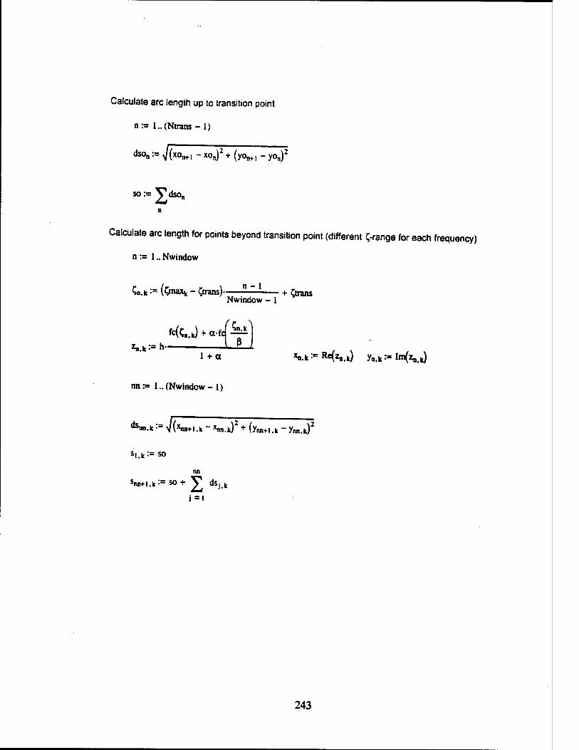
Calculate arc length up to transition point
n:= l..(Ntrans - 1)
dso„ := 7(xon+1 - xon)2 + (yon+1 - yon)2
"2 so := V dso, 'n
n
Calculate arc length for points beyond transition point (different grange for each frequency)
n := 1.. Nwindow
Sn.k := ($naxk - £trans) + örans Nwindow - 1
z„fk^h ULi 1 + a Vk - H^k) yB.k := ta(*i.k)
nn := 1.. (Nwindow - 1)
**>•" := VOWl.k - Xn„.k)2 + (yan+1,k - ymk)2
s,,k:= so
an snn+l,k:= S° + V dSjk
j=1
243
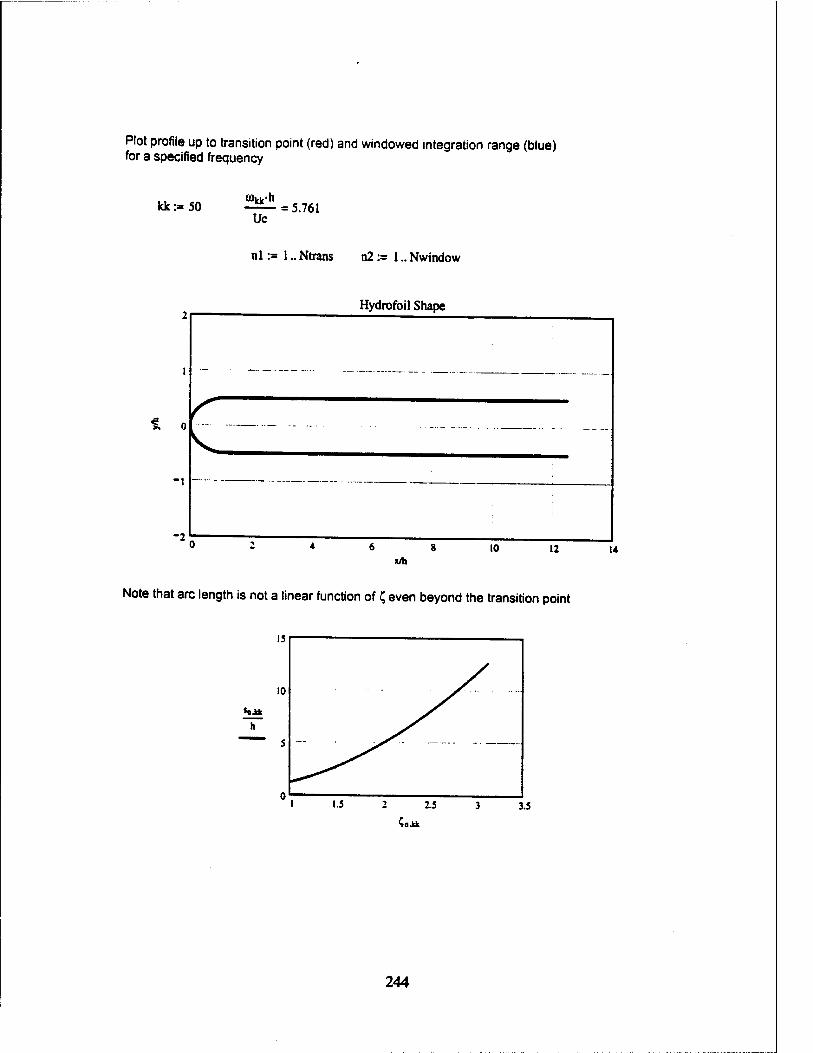
Plot profile up to transition point (red) and windowed integration range (blue) for a specified frequency
kk:=50 Uc
= 5.761
nl := 1.. Ntrans n2 := 1.. Nwindow
Hydrofoil Shape
Note that arc length is not a linear function of C, even beyond the transition point
H.tt h
244

SPECTRAL CALCULATIONS
Calculate transition zone intermittency function (eqns 3.14 and 3.15)
A := 17-so-
Yn.k := 1 - exd -cl
Uso
{■
\-0.2
ci.--4.i8 o- (j*3.v(§a£±^
'sn.k-soV
) -I
Calculate boundary layer displacement thickness and friction velocity (eqn. 3.17 and page 14)
5starn,k:= O.CMö-h.feO /u-hVM
vstar:= 0.035U
Calculate point pressure spectrum, based on Chase data (eqn. 3.16)
ctp:=0.12
Ss^.k f &«arn>k>
*PPn.k := (pvstar2)2-.Yn k - u - f^T
fl &tarn.kY : o)k—— +ap
1.5
Calculate integrand of eqn. 3.19 intn k := ^<j>ppn fc. 1 + e"l Uc J Uc Vii
nn:= 1.. (Nwindow - 1)
"Sna.k := ?nn+l.k ~ Snn.k
Apply window function wn.k •'= cos
^n Cn.k-Ctrans V
2 £maxk-$rans
intwn k := wnik.int„ik
245

Plot the integrand for a specified frequency
kk:=50 -2L_=5.761 Uc
-10
Evaluate windowed integral using trapezoidal integration
nn := 1.. (Nwindow - 1)
„ . T*l (intwnn-H.k-|-'ntWm, k)
246
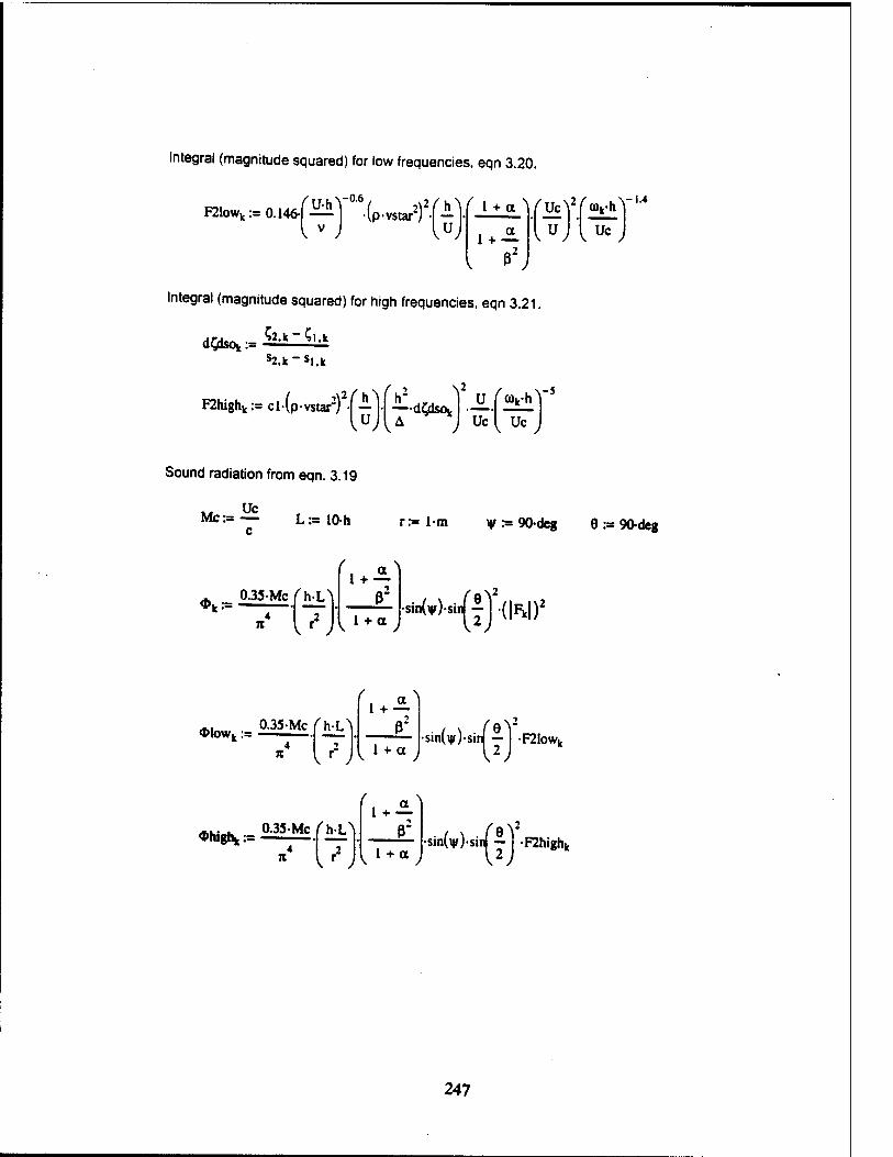
Integral (magnitude squared) for low frequencies, eqn 3.20.
F2!owk:= 0.146 Ip-vstar; • — • vv) W lti
Integral (magnitude squared) for high frequencies, eqn 3.21
^2.k ~ Cl.k
rucV u ' vUc,
-1.4
F2highk := cl-(p-vstar2) •[ — —dCdsOk A J
\5_ (cok-h
Uc ~Uc"
v-S
Sound radiation from eqn. 3.19
MC:" ~ L := 10-h r:= lm v := 90-deg 8 := 90-deg
*k:= 0.35-Mc
f a\ 1 + —
P"
11 + aJ 4 7t
in(v) sinl •*{fJ(W)!
4>lowk := 0.35-Mc fh-L^ 1 + —
V J 1 + a
•sin(\)/J-sirJ — I2,
•F21owi.
(Phighk := 0.35-Mc fh-M
v'2,
1 + — §1
# •sin(\|f)-sin| — F2highk
247
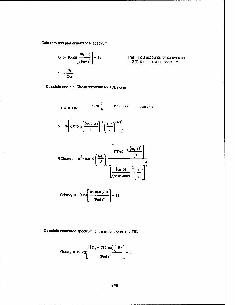
Calculate and plot dimensional spectrum
Gfc := 10-log (Pref)2
+ 11 The 11 dB accounts for conversion to G(f), the one sided spectrum.
fk:= 2-71
Calculate and plot Chase spectrum for TBL noise
CT := 0.0046 c2:=- b:=0.75 hbar:= 3 6
8:= 8 0.046-h 0.8,u<hX-0.2 rCso + ^fvu-h
*Chasev:= p -vstar -5
CTc2b : (°>k-8)4
((Ok-5)
,(hbar-vstar)_
Gchase* — 10- log 4>ChasckHz
(Prcf): + 11
Calculate combined spectrum for transition noise and TBL
Gtotalk:= 10- log T(4>k + <DChase)l-Hz
(Pref)- + 11
248
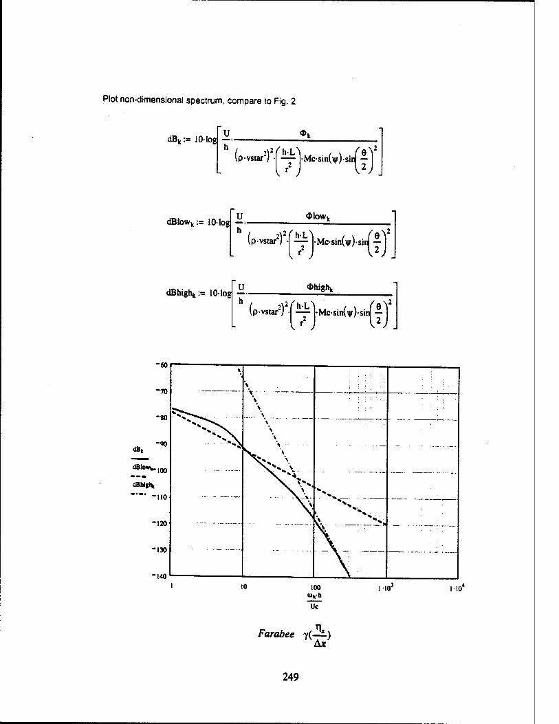
Plot non-dimensional spectrum, compare to Fig. 2
dBk:= 10-log — U
h
4>w
ip-vstar") • fh-L\
V r )
Mc-sin(v)-si <*r dBlowk:= 10-log —
U
h
4>lowk
(p-vstar2) •
V2; Mc-sin(\|/)-sin —
\2)
dBhighk:= 10-log — U
h
4>highk
->\2
(p-vstar2) fhL\
KT J
Mc-sin(v)- ■er -60
1 10
Farabee y(—) Ax
249
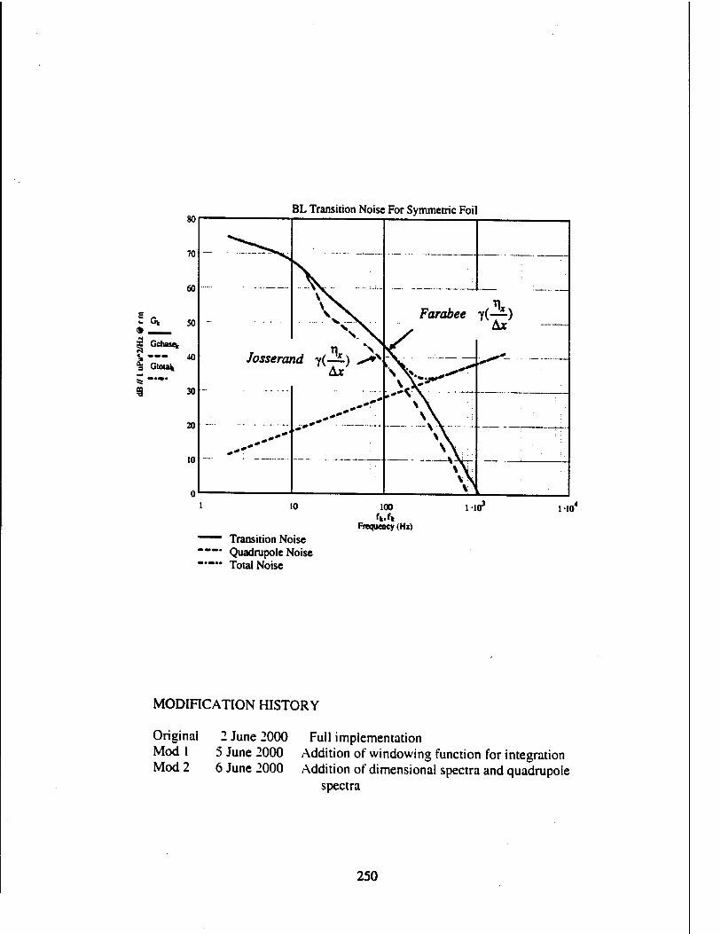
BL Transition Noise For Symmetric Foil
100
Frequency (Hz)
-"■ Transition Noise *"' Quadrupole Noise — Total Noise
I 10
MODIFICATION HISTORY
Original 2 June 2000 Full implementation Mod 1 5 June 2000 Addition of windowing function for integration Mod 2 6 June 2000 Addition of dimensional spectra and quadrupole
spectra
250
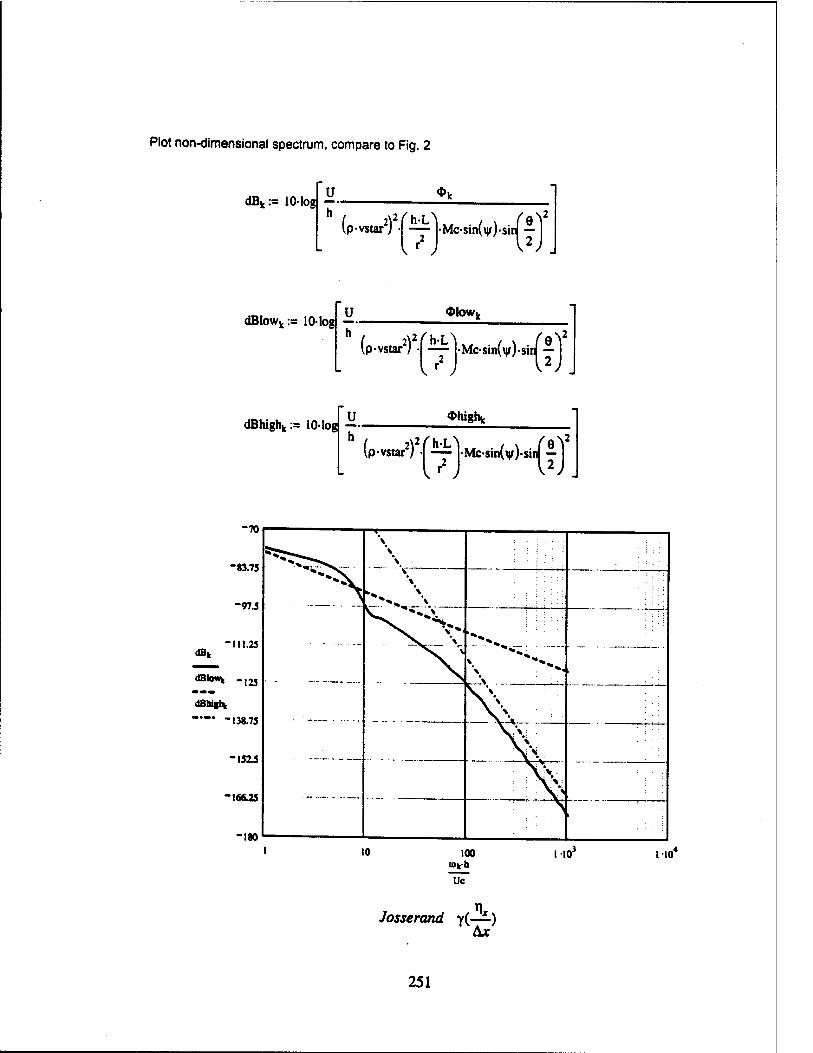
Plot non-dimensional spectrum, compare to Fig. 2
dBk:= 10-log — U
h *k
(p-vstar2) • fh-L\
,^ •Mc-sin(\|/)- "{5J
dBIowk:= 10-log U
h
$k>Wi,
(p-vstar2) • — -Mc-sinU)-sin| —
dBhighk := 10-log U
h
«thigh*
(p-vstar2) fh-L\
Kr ) Mc-sin(v)
-(«'
■70
"83.75
"97.3
-111.25 dBk
dBlowfc -125
dBtng\
—"• - 138.75
-1515
-1Ä2S
-180
NX \ ■ ; ; . ;:: rTr?
X \
10 100 iioJ 110*
Josserand y(—) Ax
251
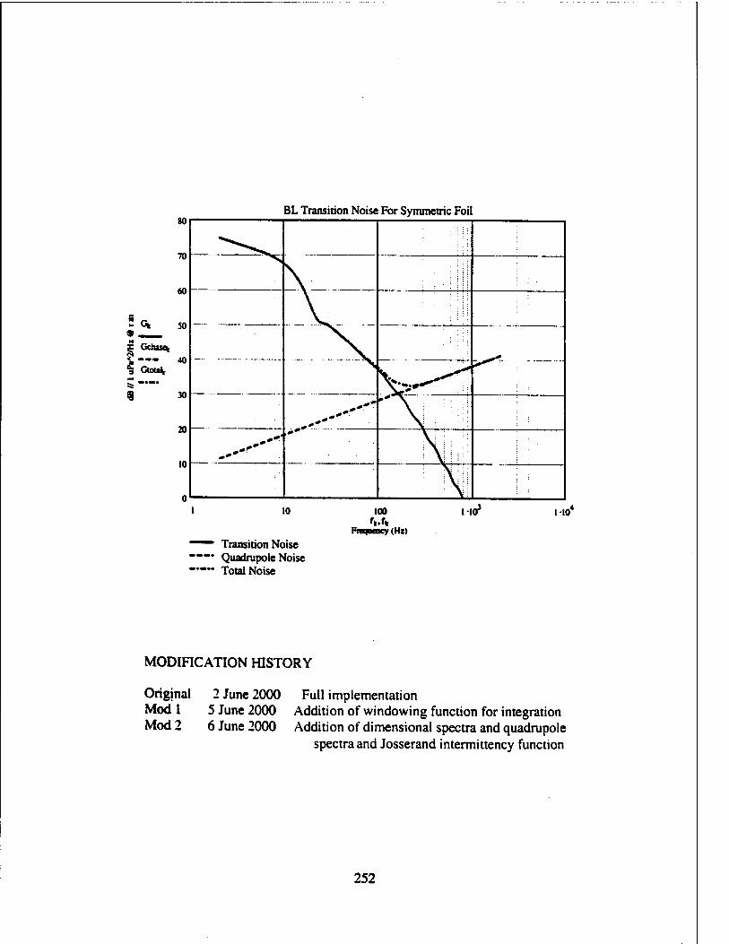
80
70
60
50
BL Transition Noise For Symmetric Foil
x Gchascfc
1, 40 % GtouV
9 30
20
10
_ ^__
„»» ! ; \j I p: ;
I 10
"~~ Transition Noise —* Quadrupole Noise —— Total Noise
100 fk.rk
Fiequcncy (Hz)
M03 I 10'
MODIFICATION HISTORY
Original Modi Mod 2
2 June 2000 Full implementation 5 June 2000 Addition of windowing function for integration 6 June 2000 Addition of dimensional spectra and quadrupole
spectra and Josserand intermittency function
252
A.6 Calculation of Boundary Layer Descriptors • AIR
Mathcadfile: TRANSITION AIR.MCD
253
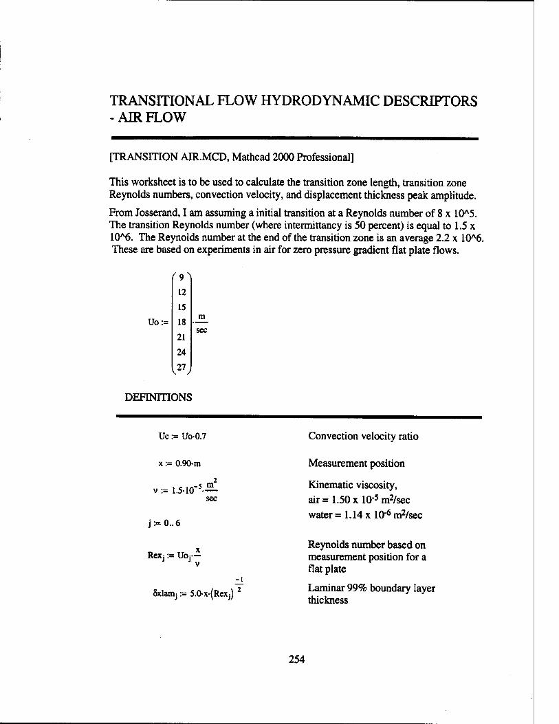
TRANSITIONAL FLOW HYDRODYNAMIC DESCRIPTORS -AIRFLOW
[TRANSITION AIR.MCD, Mathcad 2000 Professional]
This worksheet is to be used to calculate the transition zone length, transition zone Reynolds numbers, convection velocity, and displacement thickness peak amplitude.
From Josserand, I am assuming a initial transition at a Reynolds number of 8 x 10A5. The transition Reynolds number (where intermittancy is 50 percent) is equal to 1.5 x 10A6. The Reynolds number at the end of the transition zone is an average 2.2 x 10A6. These are based on experiments in air for zero pressure gradient flat plate flows.
f9l 12
15
Uo:= 18 m
21 sec
24
k27J
DEFINITIONS
Uc := Uo-0.7
x := 0.90-m
v := 1.5-H r»j£ sec
j:=0..6
Convection velocity ratio
Measurement position
Kinematic viscosity, air = 1.50 xl0"5m2/sec water = 1.14 x 10"6 n^/sec
Rexj := UOJ—
8xlanij := 5.0v(Rexj)
Reynolds number based on measurement position for a flat plate
Laminar 99% boundary layer thickness
254

Sxturbj := 0.37-x-(Rex j)
xOj := 800000
UO;
xo RexOj := UOj—l
Turbulent boundary layer thickness
Effective leading edge point of transition zone
Transition LE Reynolds number (by definition)
Axi:= Uoj,
60-(RexOj) 0.667 Length of transition zone
Chen and Thyson use 60, Josserand found 40
xoi Sstarlanij := 1.743 -
(RexOj)' 0.5
Laminar displacement thickness at LE of transition zone
xtj:= 2200000
Uo:
Effective distance at beginning of fully turbulent region
Sstarturb: := 0.046- Xti
(2200000)
Displacement thickness at beginnning of fully turbulent region
ASstarj := Sstarturbj - Sstarlanij AS* calculation
ReSstarturbj := 0.018-(ReXj)7
255
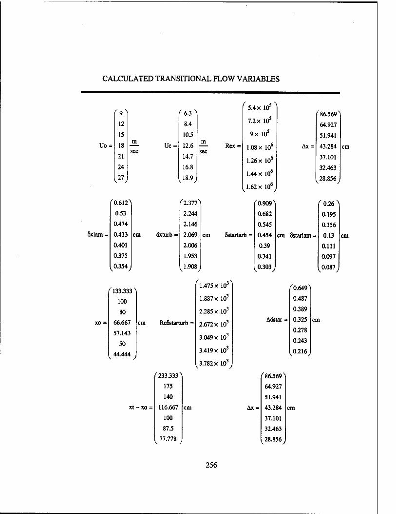
CALCULATED TRANSITIONAL FLOW VARIABLES
/ . . < \ 5.4 x 10" rg> r 6.3 ^| '86.569'
12 8.4 7.2 x 10⁵
64.927
15 10.5 9x 10⁵ 51.941
Uo = = 18 - <
21
24
01 TT — Uc = >ec
12.6
14.7
16.8
m
— Rex = sec 1.08 x 10⁶
1.26 x 10⁶
1.44 x 10⁶
Ax = 43.284
37.101
32.463
cm
,27, v ,18-9, I 28.856] k1.62x 106
;
'0.612' f 2.377 \ '0.909' ' 0.26 '
0.53 2.244 0.682 0.195
0.474 2.146 0.545 0.156
5x1am = 0.433
0.401
0.375
cm öxturb = 2.069
2.006
1.953
cm 5starturb = 0.454
0.39
0.341
cm Sstarlam = 0.13
0.111
0.097
cm
,0-354, ^1.908 / 0.303 y ^0.087,
/ 133.333
100
80
1.475 x 10^
1.887 x 10³
2.285 x 10³
'0.649'
0.487
0.389
xo = 66.667
57.143
50
cm Re&tarturb = 2.672 x 10³
3.049 x 10³
ASstar = 0.325
0.278
0.243
cm
V 44.444 ) 3.419 x 10³
<0.216,
V 3.782 x 10³y
'233.333 \ ' 86.569'
175 64.927
140 51.941
xt - xo = 116.667
100
87.5
cm Ax = 43.284
37.101
32.463
cm
^ 77.778 / 28.856 ,
256
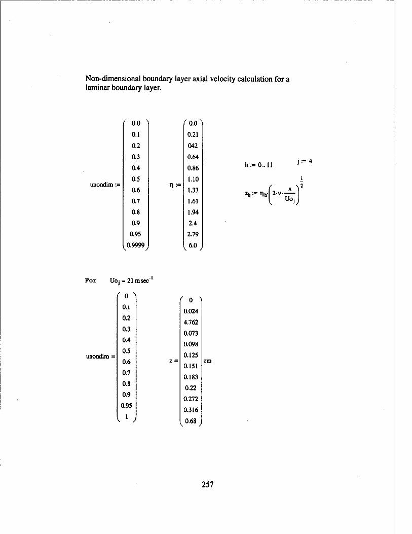
Non-dimensional boundary layer axial velocity calculation for a laminar boundary layer.
unondim :=
( 0.0 ^
0.1
0.2
0.3
0.4
0.5
0.6
0.7
0.8
0.9
0.95
0.9999
n:=
0.21
042
0.64
0.86
1.10
1.33
1.61
1.94
2.4
2.79
6.0
h:= 0.. 11 j:=4
For Uo j = 21msec"
' 0 N
' 0 ^ 0.1
0.024 0.2
4.762 0.3
0.073 0.4
0.098
unondim = 0.5
0.6 z = 0.125
0.151 0.7
0.183 0.8
0.22 0.9
0.272 0.95
0.316
< l > , °68 ,
cm
257
A.7 Calculation of Boundary Layer Descriptors - WATER
Mathcadfile: TRANSITION WATER.MCD
258
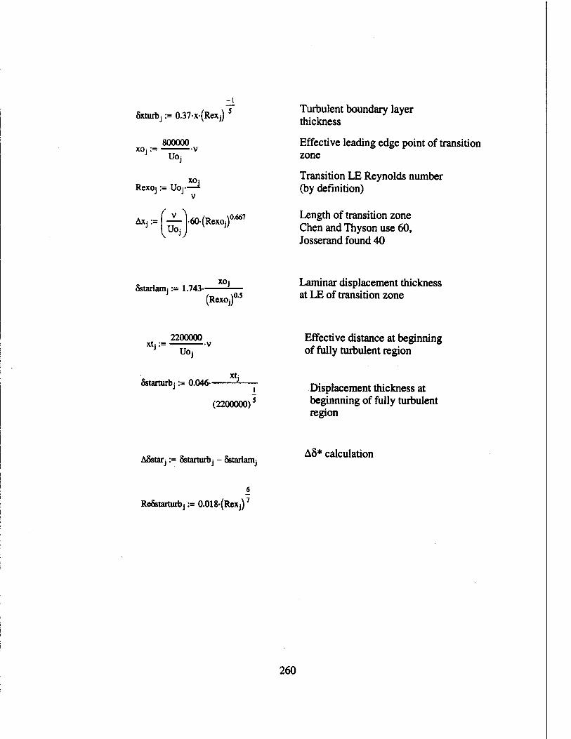
Sxturbj := 0.37-x-(Rex j) Turbulent boundary layer thickness
800000 xOj := v
1 UOj
Rexoj := UOj- XO:
Effective leading edge point of transition zone
Transition LE Reynolds number (by definition)
AXJ := 60-(RexOj) 0.667 Length of transition zone
Chen and Thyson use 60, Josserand found 40
Sstarlanij := 1.743- XO:
(Rexoj)1 0.5 Laminar displacement thickness at LE of transition zone
xtj:= 2200000
UO:
Effective distance at beginning of fully turbulent region
Sstarturbi := 0.046- Xt;
(2200000)
Displacement thickness at beginnning of fully turbulent region
A&taij := Sstarturbj - Sstarlanij A8* calculation
Re6starturbj := 0.018-(Rexj)7
260
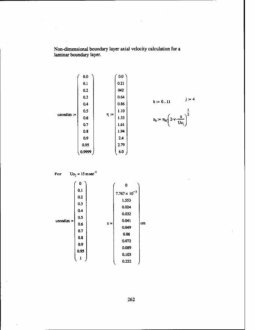
Non-dimensional boundary layer axial velocity calculation for a laminar boundary layer.
unondim :=
( 0.0 ^
0.1
0.2
0.3
0.4
0.5
0.6
0.7
0.8
0.9
0.95
0.9999
ti:=
'0.<^
0.21
042
0.64
0.86
1.10
1.33
1.61
1.94
2.4
2.79
6.0
h:= 0.. 11
Zh := 1h ( x
j:=4
l
2-v V, Uo
For
unondim =
UOJ = 15 msec
( 0 ^
0.1
0.2
0.3
0.4
0.5
0.6
0.7
0.8
0.9
0.95
1
-l
z =
0
7.767 x 10"
1.553
0.024
0.032
0.041
0.049
0.06
0.072
0.089
0.103
0.222
cm
262
A.8 Calculation of Nozzle Contour
Mathcadfile: NOZZLE CONTOUR.MCD
263
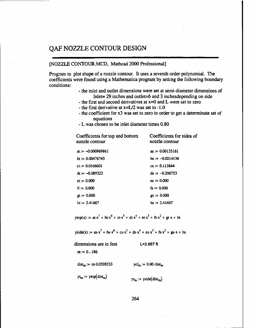
QAF NOZZLE CONTOUR DESIGN
[NOZZLE CONTOUR.MCD, Mathcad 2000 Professional]
Program to plot shape of a nozzle contour. It uses a seventh order polynomial. The coefficients were found using a Mathematica program by setting the following boundary conditions:
- the inlet and outlet dimensions were set at semi-diameter dimensions of Inlet= 29 inches and outlet=6 and 3 inchesdepending on side
- the first and second derivatives at x=0 and L were set to zero - the first derivative at x=L/2 was set to -1.0 - the coefficient for x3 was set to zero in order to get a determinate set of
equations - L was chosen to be inlet diameter times 0.80
Coefficients for top and bottom Coefficients for sides of nozzle contour nozzle contour
at := -0.000969861 as := 0.00135161
bt := 0.00476745 bs := -0.0214136
ct := 0.0166601 cs := 0.113844
dt := -0.089322 ds := -0.206753
et := 0.000 es := 0.000
ft := 0.000 fs := 0.000
gt := 0.000 gs := 0.000
ht := 2.41667 hs := 2.41667
ytop(x) := at-x7 + bt-x6 + ct-x5 + dt-x4 + etx3 + ft-x2 + gt-x + ht
yside(x) := as-x + bs-x + cs-x + ds-x + es-x + fs-x + gs-x+ hs
dimensions are in feet L=3.867 ft
m:=0..186
distn, := m-0.0208333 yclm := O.OOdistn,
yt^ytoKdisO ySm:=ySide{diSg
264
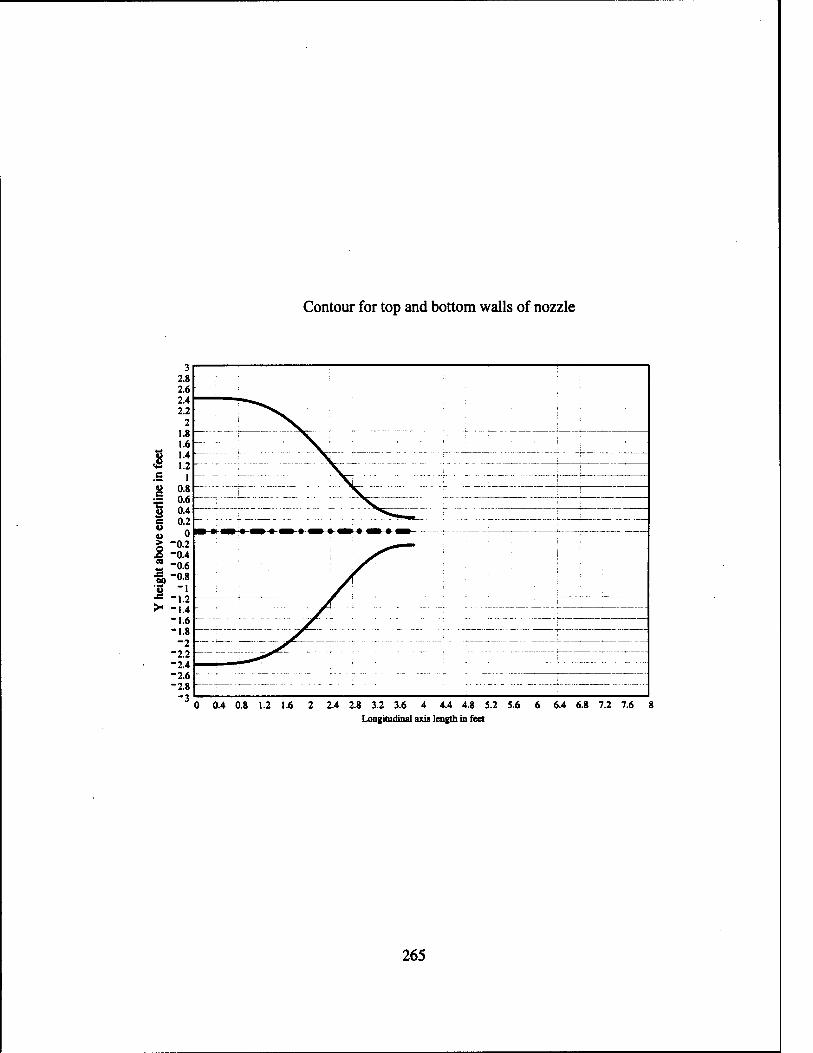
Contour for top and bottom walls of nozzle
S
op
0 0.4 0.8 1.2 1.6 2 2.4 2.8 3.2 3.6 4 4.4 4.8 5.2 5.6 6 6.4 6.8 7.2 7.6 8 Longitudinal axis length in feet
265
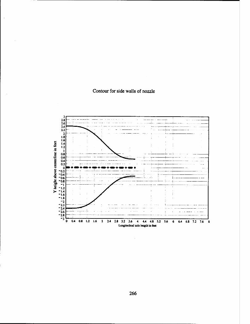
Contour for side walls of nozzle
§
§
M" 2P 3 >- -
1.4 0.8 1.2 1.6 2 2.4 2.8 3.2 3.6 4 4.4 4.8 5.2 S.6 Longitudinal axis length in feet
6 6.4 6.8 7.2 7.6 8
266
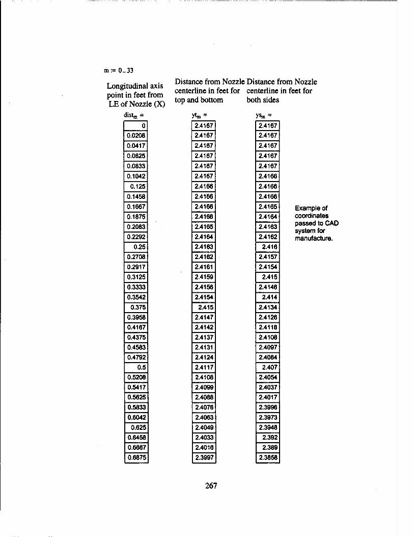
m:=0..33
Longitudinal axis point in feet from LE of Nozzle (X)
distn, =
Distance from Nozzle Distance from Nozzle centerline in feet for centerline in feet for top and bottom both sides
0.0208
0.0417
0.0625
0.0833
0.1042
0.125
0.1458
0.1667
0.1875
0.2083
0.2292
0.25
0.2708
0.2917
0.3125
0.3333
0.3542
0.375
0.3958
0.4167
0.4375
0.4583
0.4792
OS
0.5208
0.5417
0.5625
0.5833
0.6042
0.625
0.6458
0.6667
0.6875
ytm = 2.4167
2.4167
2.4167
2.4167
2.4167
2.4167
2.4166
2.4166
2.4166
2.4166
2.4165
2.4164
2.4163
2.4162
2.4161
2.4159
2.4156
2.4154
2.415
2.4147
2.4142
2.4137
2.4131
2.4124
2.4117
2.4108
2.4099
2.4088
2.4076
2.4063
2.4049
2.4033
2.4016
2.3997
ysm = 2.4167
2.4167
2.4167
2.4167
2.4167
2.4166
2.4166
2.4166
2.4165
2.4164
2.4163
2.4162
2.416
2.4157
2.4154
2.415
2.4146
2.414
2.4134
2.4126
2.4118
2.4108
2.4097
2.4084
2.407
2.4054
2.4037
2.4017
2.3996
2.3973
2.3948
2.392
2.389
2.3858
Example of coordinates passed to CAD system for manufacture.
267
A.9 Calculation of Measurement Errors from a Two Microphone Intensity Probe
Mathcadfile: INTENERROR.MCD
268
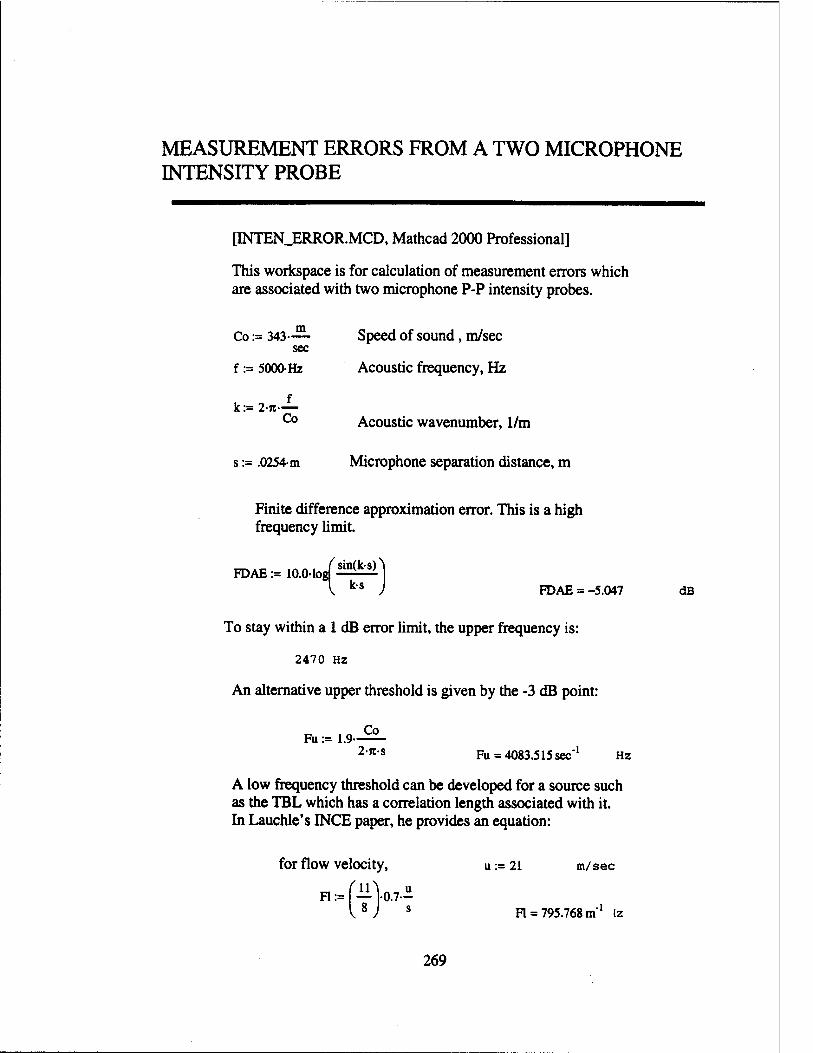
MEASUREMENT ERRORS FROM A TWO MICROPHONE INTENSITY PROBE
[INTEN_ERROR.MCD, Mathcad 2000 Professional]
This workspace is for calculation of measurement errors which are associated with two microphone P-P intensity probes.
Co := 343— Speed of sound, m/sec sec
f := 5000Hz Acoustic frequency, Hz
k := 2-71-— Co Acoustic wavenumber, 1/m
s := .0254m Microphone separation distance, m
Finite difference approximation error. This is a high frequency limit.
\ k-s ) FDAE =-5.047 dB
To stay within a 1 dB error limit, the upper frequency is:
2470 Hz
An alternative upper threshold is given by the -3 dB point:
, n Co Fu := 1.9 2Tt-s Fu = 4083.515 s«:'1 Hz
A low frequency threshold can be developed for a source such as the TBL which has a correlation length associated with it. In Lauchle's INCE paper, he provides an equation:
for flow velocity, u := 21 m/sec
u H,,T 0.7-
s Fl = 795.768 m'1 Iz
269
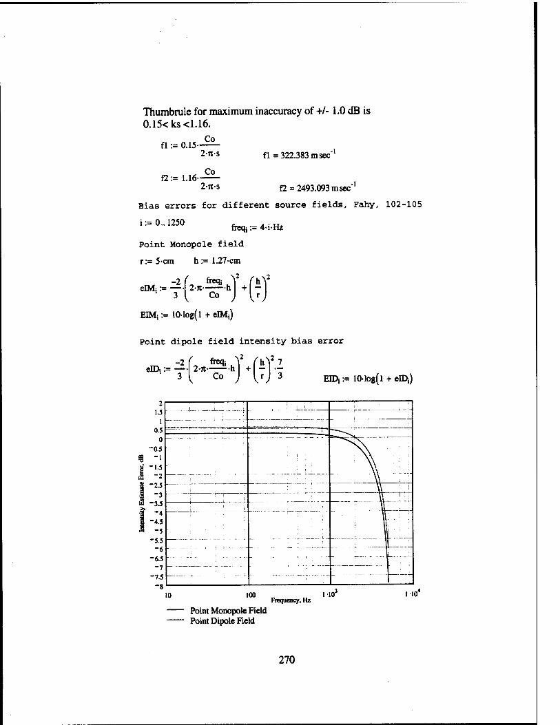
Thumbrule for maximum inaccuracy of +/-1.0 dB is 0.15<ks<1.16.
Co fl := 0.15-
f2 := 1.16
2-n-s
Co
2-n-s
fl = 322.383 msec
f2 = 2493.093 msec
Bias errors for different source fields, Fahy, 102-105
I .— \J.. li.J\l fireqj = 4-i-Hz
Point Monopole field
r:= 5-cm h := 1.27cm
-2 eIM::=
3 2-n h
% ar EIMi := 101og(l + elMj)
Point dipole field intensity bias error
-2( fieq, V (hV? en>. := — 2-n h + - --
3 Co r 3 FJD-,:= 101og(l + elDi)
Frequency, Hz 110
Point Monopole Field Point Dipole Field
270
APPENDIX B
QUIET AIRFLOW FACILITY DEVELOPMENT
This appendix provides some historical perspective of development efforts for the
Quiet Airflow Facility. The facility has progressed through many stages during the
several years covered by this investigation. All of the efforts have been focused on
reducing the background noise levels. Section 5.1 describes the current facility while this
appendix describes interim configurations and data acquisition tools.
This facility is basically a quieted air source connected to a flow management
nozzle. The original, symmetric nozzle was fitted with an internal contoured ramp to
create a semi-circular orifice rather than the circular one that previously existed. This
nozzle formed an open jet with an opening axis perpendicular to a planar baffle. A plate
mounted in the semi-circular orifice formed a wall jet over the test plate. This
configuration is shown in Figure B.l.
B.l Power Source Improvements
The Buffalo Forge centrifugal blower was originally powered by a 20 HP AC
motor driven by a Borg-Warner inverter. This has been replaced by an ABB inverter.
This was necessary because of the lack of spare parts for the Borg-Warner system. This
old inverter had been used a long as possible because it produced a "sloppy" excitation
that was a much smoother sinusoid than the modem, six-step, digitally generated
271
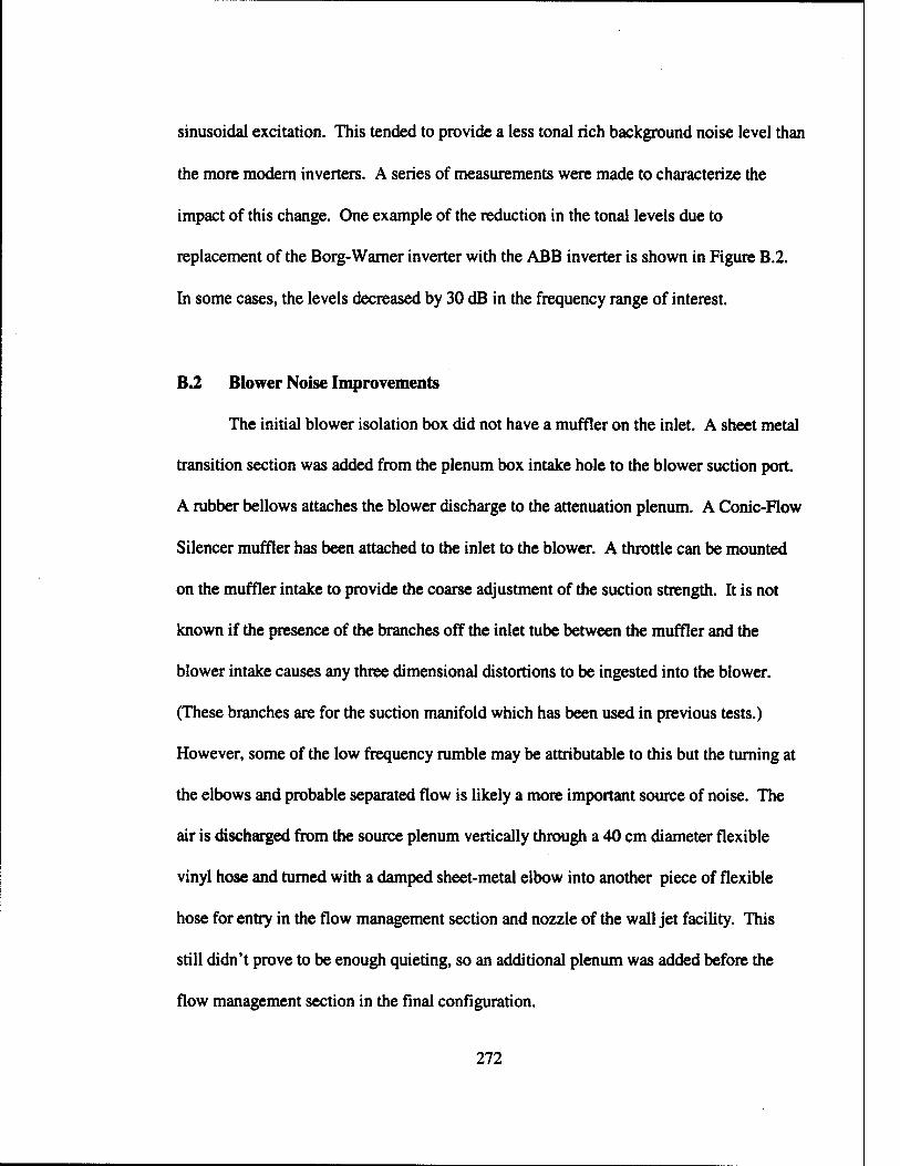
sinusoidal excitation. This tended to provide a less tonal rich background noise level than
the more modern inverters. A series of measurements were made to characterize the
impact of this change. One example of the reduction in the tonal levels due to
replacement of the Borg-Warner inverter with the ABB inverter is shown in Figure B.2.
In some cases, the levels decreased by 30 dB in the frequency range of interest.
B.2 Blower Noise Improvements
The initial blower isolation box did not have a muffler on the inlet. A sheet metal
transition section was added from the plenum box intake hole to the blower suction port.
A rubber bellows attaches the blower discharge to the attenuation plenum. A Conic-Flow
Silencer muffler has been attached to the inlet to the blower. A throttle can be mounted
on the muffler intake to provide the coarse adjustment of the suction strength. It is not
known if the presence of the branches off the inlet tube between the muffler and the
blower intake causes any three dimensional distortions to be ingested into the blower.
(These branches are for the suction manifold which has been used in previous tests.)
However, some of the low frequency rumble may be attributable to this but the turning at
the elbows and probable separated flow is likely a more important source of noise. The
air is discharged from the source plenum vertically through a 40 cm diameter flexible
vinyl hose and turned with a damped sheet-metal elbow into another piece of flexible
hose for entry in the flow management section and nozzle of the wall jet facility. This
still didn't prove to be enough quieting, so an additional plenum was added before the
flow management section in the final configuration.
272
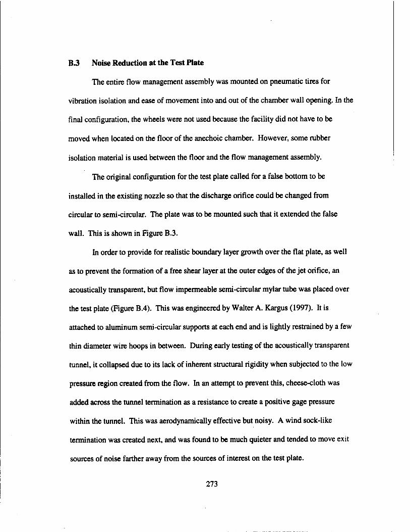
B 3 Noise Reduction at the Test Plate
The entire flow management assembly was mounted on pneumatic tires for
vibration isolation and ease of movement into and out of the chamber wall opening. In the
final configuration, the wheels were not used because the facility did not have to be
moved when located on the floor of the anechoic chamber. However, some rubber
isolation material is used between the floor and the flow management assembly.
The original configuration for the test plate called for a false bottom to be
installed in the existing nozzle so that the discharge orifice could be changed from
circular to semi-circular. The plate was to be mounted such that it extended the false
wall. This is shown in Figure B.3.
In order to provide for realistic boundary layer growth over the flat plate, as well
as to prevent the formation of a free shear layer at the outer edges of the jet orifice, an
acoustically transparent, but flow impermeable semi-circular mylar tube was placed over
the test plate (Figure B.4). This was engineered by Walter A. Kargus (1997). It is
attached to aluminum semi-circular supports at each end and is lightly restrained by a few
thin diameter wire hoops in between. During early testing of the acoustically transparent
tunnel, it collapsed due to its lack of inherent structural rigidity when subjected to the low
pressure region created from the flow. In an attempt to prevent this, cheese-cloth was
added across the tunnel termination as a resistance to create a positive gage pressure
within the tunnel. This was aerodynamically effective but noisy. A wind sock-like
termination was created next, and was found to be much quieter and tended to move exit
sources of noise farther away from the sources of interest on the test plate.
273

The sidewall contamination is reduced by incorporation of suction along the test
plate following Motohashi and Blackwelder (1983). A narrow (6 mm) slot along the side
of the test plate provides a gap in which some of the over-pressurized air within the mylar
tube is allowed to discharge to eliminate secondary flows at the plate-tube junction.
Therefore, a much greater percentage of the flow over the test plate remains laminar
before wall contamination extends to the center of the plate.
Care was taken to make all corners within the settling chamber and nozzle as
smooth as possible to help maintain laminar irrotational flow. Initial measurements
indicated that a maximum velocity of 31.7 m/sec at the exit could be achieved. By
surveying over the plate with a capillary total head tube on a stethoscope (Figure 5.14),
the bursting typical of transition was found to occur about half way down the plate which
indicated the beginning of natural transition. Subsequent measurements with a tuft wand
indicated that small corner vortices were being created inside the nozzle at the junction of
the nozzle wall and the flat bottom. To eliminate this, the test plates were redesigned to
include an extension of the plate 15 cm into the nozzle. The entire plate was raised about
2.5 cm from its previous position to create a 1.2 cm high by 30.5 cm wide duct below the
plate through which wall flow (including the vortices) could be removed via a suction
manifold. Suction for flow management on the test plate was provided by the blower
intaking air from a 10 cm hose attached to the duct between the muffler and the rubber
isolation hose into the blower. The manifold was developed to provide a more even
suction distribution. This is shown in Figure B.4. The manifold itself is shown in Figure
B.5. The end plate is removed in one of the photographs to show the rod mechanism for
274
opening and closing the orifices with wooden cones.
When designing the extension of the test plate into the nozzle care was taken to
avoid leading edge separation and premature transition by incorporating a 4:1 elliptical
leading edge (as suggested by Gad-el-Hak et al., 1981) and the windsock resistance at the
end of the plate. This assured that the stagnation line near the leading edge was on the
upper, working surface.
Provision was made for either mechanical or wind puff turbulent structure trips to
be attached below the test plate and reside in the laminar region.
Despite all of this effort, it was determined that this configuration did not meet the
low background noise levels required to make transition zone noise measurements.
Figure B.6 shows a sound pressure level measurement made above a natural transition
zone with a flow velocity of 11.8 m/s. An early version of GLPROG81 was used to
calculate predicted levels for transition noise. This required the rather unlikely values of
normalized rise time to be between 0.05 and 0.15 in order to match the measurement.
Given the shape of the spectrum, it is likely that other contaminating noise sources where
measured. Figures B.7 provides the prediction for the same flow conditions using the
latest version of GLPROG81.
B.4 Relocation of Test Section and New Nozzle Design
After the success of Brungart (1997) operating with the flow management section
and square nozzle located in the anechoic chamber (Figure B.8), it was decided to keep
this configuration intact and add an additional plenum. The intention was to further
275

reduce the low frequency background noise.
However, the 46 cm x 46 cm outlet nozzle needed to be replaced with one that
provided a 15.2 cm x 30.5 cm outlet. The design of this nozzle is described in section
5.1.3.
B.5 Diffuser Design
A new diffuser needed to be designed since the Brungart configuration did not
utilize one. The intent was to slow the flow and move any possible trailing edge noise
sources as far as possible from the test section measurements.
Kline (1959) and Kline, et al. (1959) were used to design the diffuser. The
Mathcad file for calculating and specifying the nozzle contours is provided in section A.6.
In the design of a straight walled diffuser, one needs to be aware of the potential for a
stalled flow to develop in the diffuser. Kline (1959) provided a criterion for determining
if stall might exist. This is shown in Figure B.9 as the line on the plot. The diffuser went
through several deign iterations which are listed in Figure B.9. The open circles refer to
the design condition for the side walls and the dark circles refer to the top and bottom
walls. A natural diffusion angle, 0, of 7 degrees was designed first; however, a steady
stall condition resulted. The diffuser length was decreased by 30% but the stall was still
present The diffuser was then reconstructed with a 4.5 degree diffuser angle. Transitory
stall was seen depending on the measurement openings in the test section. When the
Soundcoat <D foam was installed, this reduced the effective angle to 3.5 degrees.
Transitory stall still occurs at times but it is a very weak circulation. Barlow et al. (1999)
276
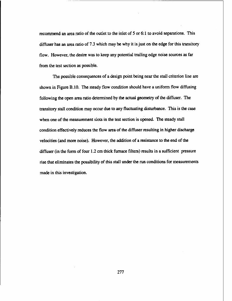
recommend an area ratio of the outlet to the inlet of 5 or 6:1 to avoid separations. This
diffuser has an area ratio of 7.3 which may be why it is just on the edge for this transitory
flow. However, the desire was to keep any potential trailing edge noise sources as far
from the test section as possible.
The possible consequences of a design point being near the stall criterion line are
shown in Figure B.10. The steady flow condition should have a uniform flow diffusing
following the open area ratio determined by the actual geometry of the diffuser. The
transitory stall condition may occur due to any fluctuating disturbance. This is the case
when one of the measurement slots in the test section is opened. The steady stall
condition effectively reduces the flow area of the diffuser resulting in higher discharge
velocities (and more noise). However, the addition of a resistance to the end of the
diffuser (in the form of four 1.2 cm thick furnace filters) results in a sufficient pressure
rise that eliminates the possibility of this stall under the run conditions for measurements
made in this investigation.
277
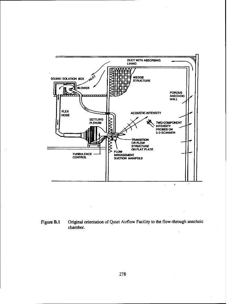
TURBULENCE CONTROL
TWO-COMPONENT INTENSITY PROBES ON 3-0 SCANNER
-TRANSITION OR FLOW STRUCTURE ON FLAT PLATE
FLOW MANAGEMENT SUCTION MANIFOLD
Figure B.l Original orientation of Quiet Airflow Facility to the flow-through anechoic chamber.
278
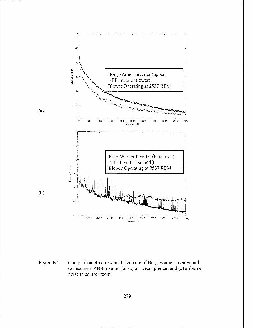
(a)
Borg-Warner Inverter (upper) ABB Inverter (lower) Blower Operating at 2537 RPM
v-VivA./"^ ^
200 -100 BOO 800 1000 1200 1400 1600 1800 2000 Frequency. H2
(b)
Borg-Wamer Inverter (tonal rich) ABB Inverter (smooth) Blower Operating at 2537 RPM
0 1000 2000 3000 4000 5000 6000 7000 8000 9000 10000 Frequency, Hz
Figure B. 2 Comparison of narrowband signature of Borg-Warner inverter and replacement ABB inverter for (a) upstream plenum and (b) airborne noise in control room.
279
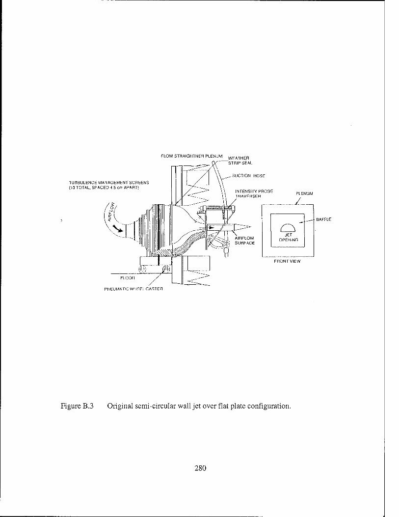
FLOW STRAIGHTNER PLENUM WEATHER STRIP SEAL
SUCTION HOSE
TURBULENCE MANAGEMENT SCREENS (10 TOTAL. SPACED 4.5 cm APART)
BAFFLE
PNEUMATIC WHEEL CASTER
Figure B.3 Original semi-circular wall jet over flat plate configuration.
280
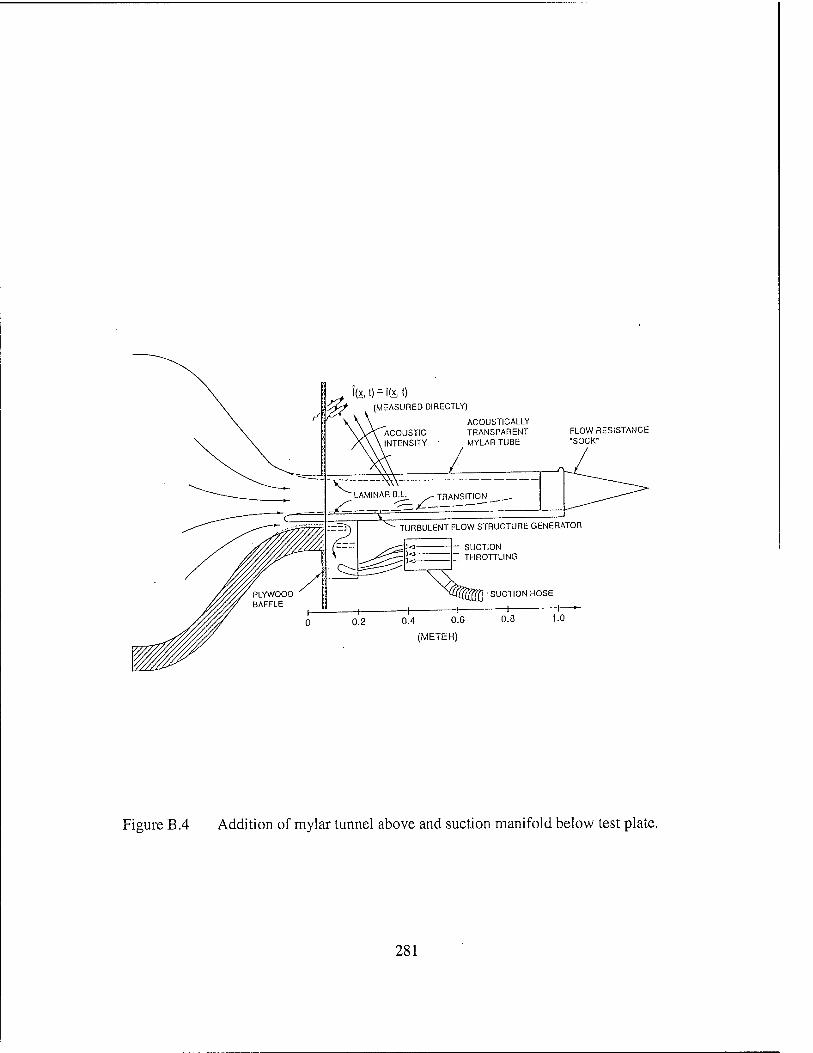
I(x,l) = l(x.l) (MEASURED DIRECTLY)
ACOUSTICALLY TRANSPARENT MYLAR TUBE
FLOW RESISTANCE ■SOCK-
TURBULENT FLOW STRUCTURE GENERATOR
SUCTION _ THROTTLING
0.4 0.6
(METER)
■SUCTION HOSE
1 1 0.8 1.0
Figure B.4 Addition of mylar tunnel above and suction manifold below test plate.
281
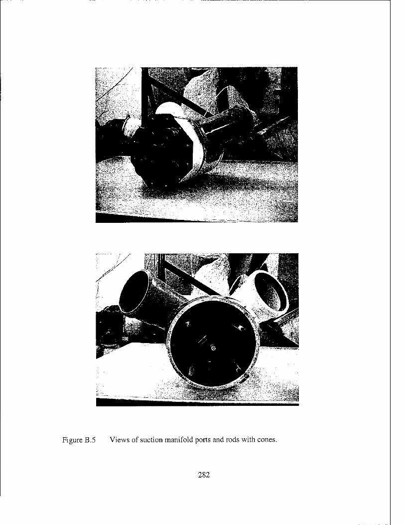
Figure B.5 Views of suction manifold ports and rods with cones.
282

50
N I
o CM
m X) _i UJ > UJ _l
UJ DC
w W ULI CC a. a z: o
-10
tj Uc/Ax = 0.05 = 0.15
MEASURED
2 3
FREQUENCY (kHz)
Figure B.6 Measured sound pressure level for assembly in control room running at U„=ii.S m/s compared to GLPROG81 predictions for uct/Ax=0A5 and uct/zfx=0.05.
283
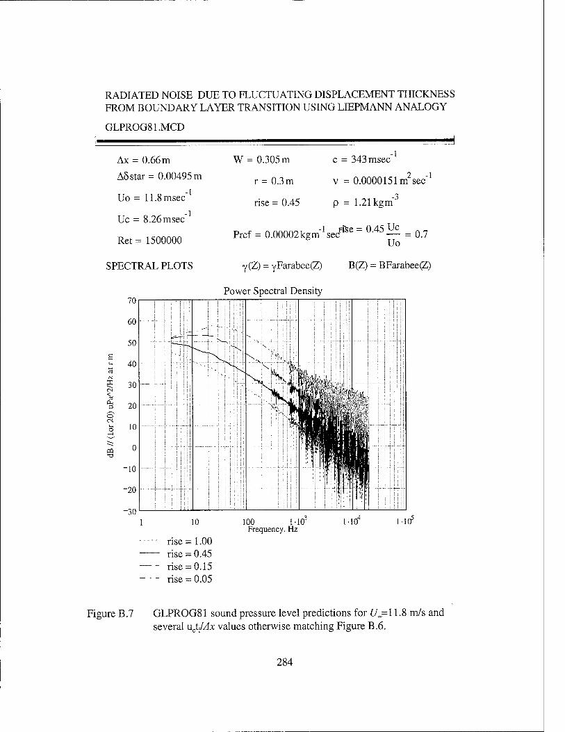
RADIATED NOISE DUE TO FLUCTUATING DISPLACEMENT THICKNESS FROM BOUNDARY LAYER TRANSITION USING LIEPMANN ANALOGY
GLPROG81.MCD
Ax = 0.66 m
A5star= 0.00495 m -1
-l
Uo = 11.8 msec
Uc = 8.26 msec
Ret = 1500000
SPECTRAL PLOTS
W = 0.305 m
r = 0.3m
rise = 0.45
c = 343 msec 1
v =0.0000151m2 sec"1
-3
Pref = 0.00002 kgm sec
p = 1.21 kgm
1 rfce = 0.45 Uc Uo
0.7
Y(Z) = YFarabee(Z) B(Z) = BFarabee(Z)
Power Spectral Density
< a, a o
■a
10
rise = 1.00 rise - 0.45 rise = 0.15 rise = 0.05
100 1 10 Frequency, Hz
Figure B.7 GLPROG81 sound pressure level predictions for U=l 1.8 m/s and several uct/zfx values otherwise matching Figure B.6.
284
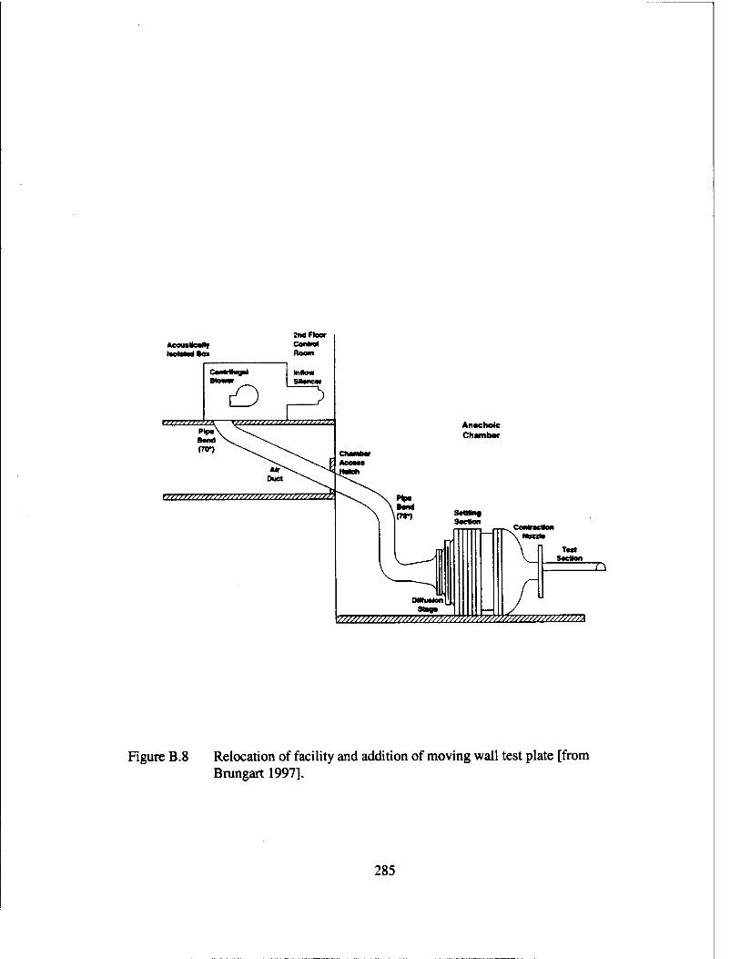
2nd ROOT
COAfeW Room
S»»nC«
cO Z3 tzzzzzzzzzz >>>>>>/>j;>n>i/j/j/.
r/////////////////j;/»;////t///»?r77>
Anvcholc Chamber
TMt
ID
\M»MM»»»M»W;»»>»»>»/WM»M/»»M
Figure B.8 Relocation of facility and addition of moving wall test plate [from Brungart 1997].
285
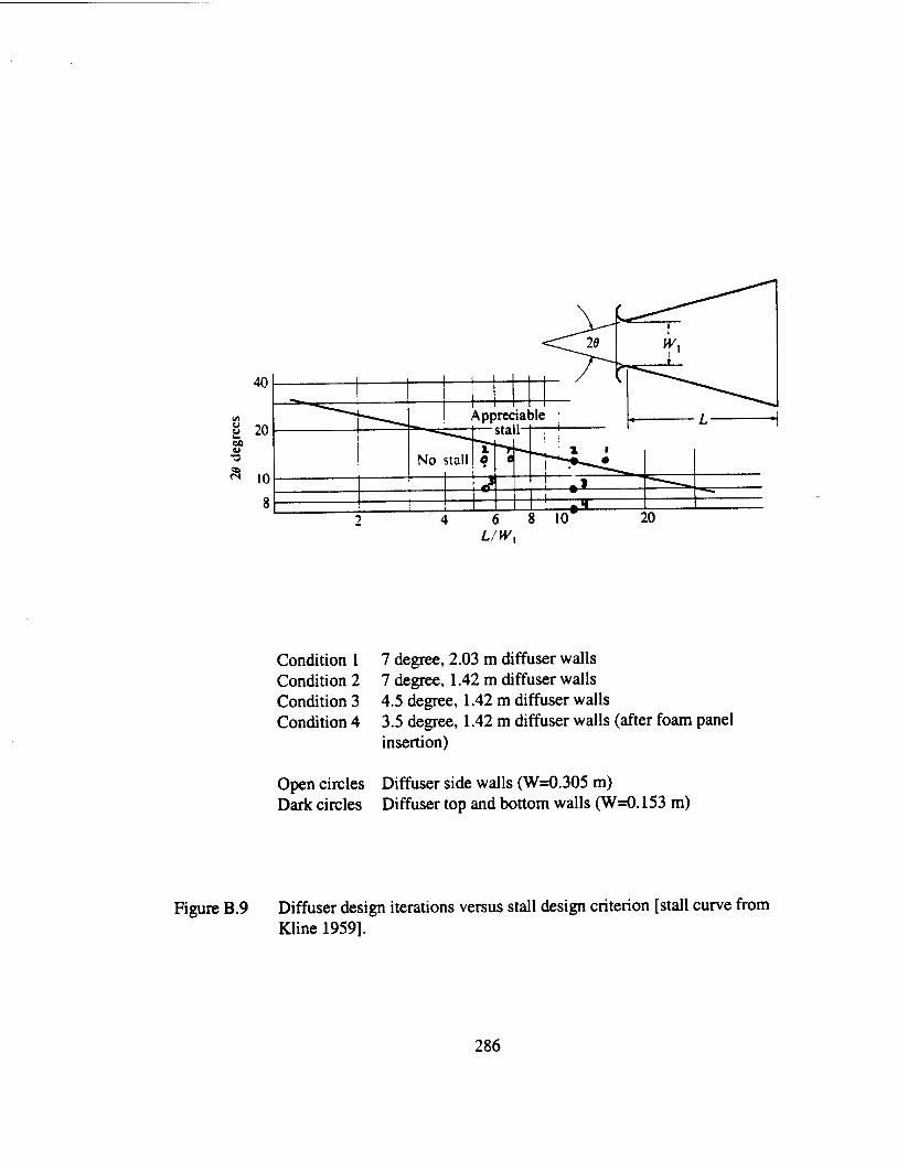
SS 20- BO u
Condition 1 7 degree, 2.03 m diffuser walls Condition 2 7 degree, 1.42 m diffuser walls Condition 3 4.5 degree, 1.42 m diffuser walls Condition 4 3.5 degree, 1.42 m diffuser walls (after foam panel
insertion)
Open circles Diffuser side walls (W=0.305 m) Dark circles Diffuser top and bottom walls (W=0.153 m)
Figure B.9 Diffuser design iterations versus stall design criterion [stall curve from Kline 1959].
286
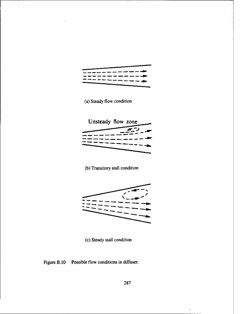
(a) Steady flow condition
Unsteady flow zone
(b) Transitory stall condition
(c) Steady stall condition
Figure B. 10 Possible flow conditions in diffuser.
287
APPENDIX C
REAL-TIME ACOUSTIC INTENSITY SIGNAL PROCESSING
This appendix describes the real-time acoustic active intensity signal processing
performed during the air flow experiment. The processing uses inputs from two
microphones using a pressure - pressure (P-P) configuration. The two pressures are
averaged to represent the pressure at a location intermediate to the two microphones and
acoustic particle velocity is derived by a finite difference integration of the pressures.
This is predominately performed in a time-averaged sense. Procedures, governing
equations, and uncertainty analysis are well documented in Fahy (1989).
The general concept for making measurements of the acoustic signature of the
transition zone or individual turbulent spots is shown in Figure C.l. Transition is allowed
to occur naturally or a laminar flow condition is set and a stimulation is used to trigger a
turbulent spot. This stimulation can be an acoustic impulse from a speaker or a
mechanically generated air puff. A flush mounted hot film is used to provide a spectral
conditioning signal. The microphones may be flush mounted as shown in the figure or
mounted outside of the tunnel. The idea is to have the microphone separation large
enough so that there will be little correlated flow noise between them. Also by orienting
the two microphones in a line normal to the tunnel axis, the null of the cosine directivity
pattern associated with the intensity probe will reject plane wave tunnel noise propagating
along the tunnel axis.
288
C.l Time-Averaged Intensity Processing
The traditional method of time-averaged processing a P-P probe is shown in
Figure C.2. The active intensity for a time-stationary sound field is obtained from:
7"(ö>) = ~{-^)Im{G^m (CD
An alternative method often used for handheld 1/3 octave intensity measurement
devices is shown in Figure C.3. Here sum and differencing is done to the two analog
microphone signals before they are passed through 1/3 octave filters and the difference
signal is analog integrated. Analog-to-digital conversion is then performed before
multiplication and division by p0d. Averaging is often then performed.
C.2 Real-Time Intensity Processing
An approximation for the instantaneous particle velocity taken from the
component of the pressure gradient in a direction n is given by:
un(t) ~~ -(-L) /[£Ö>]* (C.2)
With In(t) = p(t) u„(t), the instantaneous active intensity component is approximated by:
W a -(T^)IPI<')+P2«] /IP1W-P2W]* (CJ)
An example of the analog integrator needed to implement Equation C.3 is given in
Figure C.4.
289
The portions of the processing diagram prior to the A/D conversion have been
implemented in an electronic circuit. The design of this circuit and its fabrication was
performed by Todd D. Batzel of the Applied Research Laboratory at Penn State. The
circuit diagram is shown in Figure C.5. The component layout is provided in Figure C.6.
This circuit has two analog inputs which can be up to 5 volts. A high pass filter
has been implemented with a cut-off at 30 Hz. The filter is a fourth order Bessel filter
with linear phase (Burr-Brown Universal Active Filter, UAF42G). This was chosen for
this particular application in order to remove some low frequency tunnel noise that
otherwise would have used up about 40 dB of dynamic range. The gains in the circuit are
as follows:
multiply by 250 in input
multiply by 295 in integrator
divide by 10 in multiplier
total gain = multiply by 7375 or 38.7 dB
A reset button is installed for the integrator to allow re-zeroing in case of a built up bias.
The circuit can be powered by two onboard 9V batteries or an AC adapter.
The remainder of the processing is performed in the DSP Technologies, Inc
SigLab ® 20-42 dynamic signal processor which uses The Mathworks, Inc MATLAB ®
software.
It is important for the signal processing of a P-P probe to have two channels well
matched in amplitude and phase. The output of the real-time intensity circuit should be
zero for the same signal being input to both channels. Any residual intensity is an
290
indication of an error which consists of random error and bias. The "residual intensity"
as compared to the same signal input to channels 1 and 2 of the intensity circuit is shown
in Figure C.7. The upper plot shows the phase and amplitude matching of the input
signals even with any channel mismatch on the SigLab analyzer. The wide variation in
phase and amplitude with frequency indicate problems in the circuitry that were not able
to be overcome without a complete redesign. The impact can be seen in Figure C.8 with
a comparison of the same measurement for the case of a fully turbulent flow condition
between the time-averaged active intensity method and the real-time intensity circuit. A
contributing problem may be the closeness of the probe to the source in these
measurements. The highly reactive acoustic field may not be conducive to the real-time
measurement.
C J Conditioning with a Shear Stress Sensor
It is desired to apply the power of coherent output processing to the acoustic
measurements. In this case, it is assumed that shear stress due to passage of a turbulent
spot is caused by the same physical phenomenon (i.e. growth of the turbulent spot) that
results in acoustic radiation (represented by the transfer function h(x). Therefore, there
should be coherence between thiose signals. The noise associated with each sensor is
assumed to be uncorrelated. These are identified in Figure C.9. It has been demonstrated
in other experiments that the shear stress sensor (hot film) is insensitive to background
acoustic noise.
This represents a single-input / single-output problem. The measured coherence
291
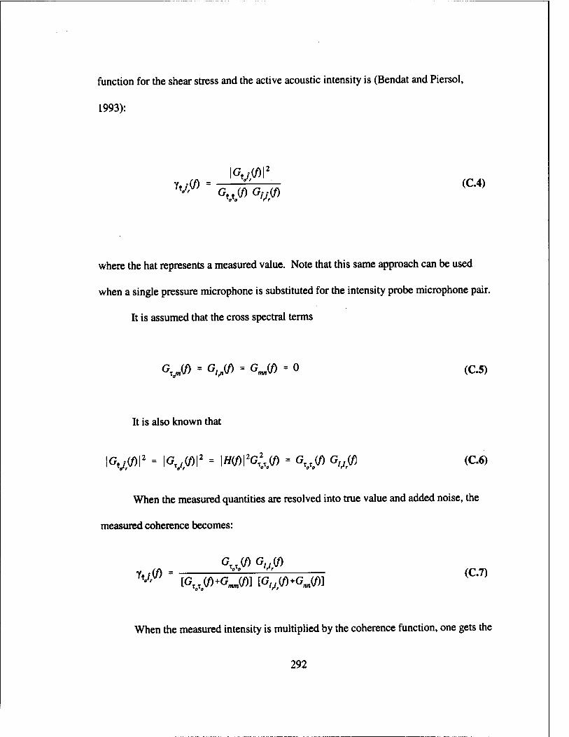
function for the shear stress and the active acoustic intensity is (Bendat and Piersol,
1993):
\Gu(f)\2
y.(/) = ZL (C.4)
where the hat represents a measured value. Note that this same approach can be used
when a single pressure microphone is substituted for the intensity probe microphone pair.
It is assumed that the cross spectral terms
It is also known that
|Gv;(/)|2 = \GxJ(f)\* = \H(f)\%o(f) = GTZ(f) Glrl(fl (C.6)
When the measured quantities are resolved into true value and added noise, the
measured coherence becomes:
v,</) = [^(O+GIWI iGvffi+Gjm (C7)
When the measured intensity is multiplied by the coherence function, one gets the
292
equation:
v,w'%» - «„.» t^&5ji <™>
Therefore, a good estimate of the true spectrum of the acoustic intensity is obtained when
Gmm(f)«Gr0T0(f) regardless of the amplitude of Gnn(0. Josserand's prior measurements
(Josserand 1986) and intermittency measurements made during this investigation have
shown that the shear stress measurements have a very high signal- to-noise ratio and
should meet the criterion well.
293
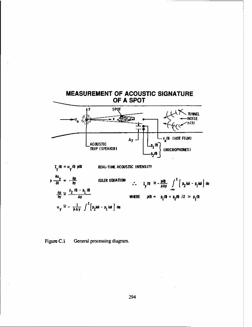
MEASUREMENT OF ACOUSTIC SIGNATURE OF A SPOT
*:\ *U0 Vk>
£UO\ TUNNEL *X. —NOISE
Iy(8=uy(t)p(0
? dt dy
ACOUSTIC "TRIP (SPEAKER!
REAL-TIME ACOUSTIC INTENSITY
EULER EQUATION
I— T(8 I HOT FILM) o
(MICROPHONES!
-oo
WHERE (Xtt = Pj(» ♦ i^ra /2 - Pj(0 dy " Ay
Figure C.l General processing diagram.
294
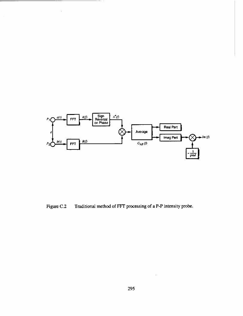
GABW
Real Part } ImagPart |^-»»(^-»-/m <f>
1 ^1 pad I
Figure C.2 Traditional method of FFT processing of a P-P intensity probe.
295
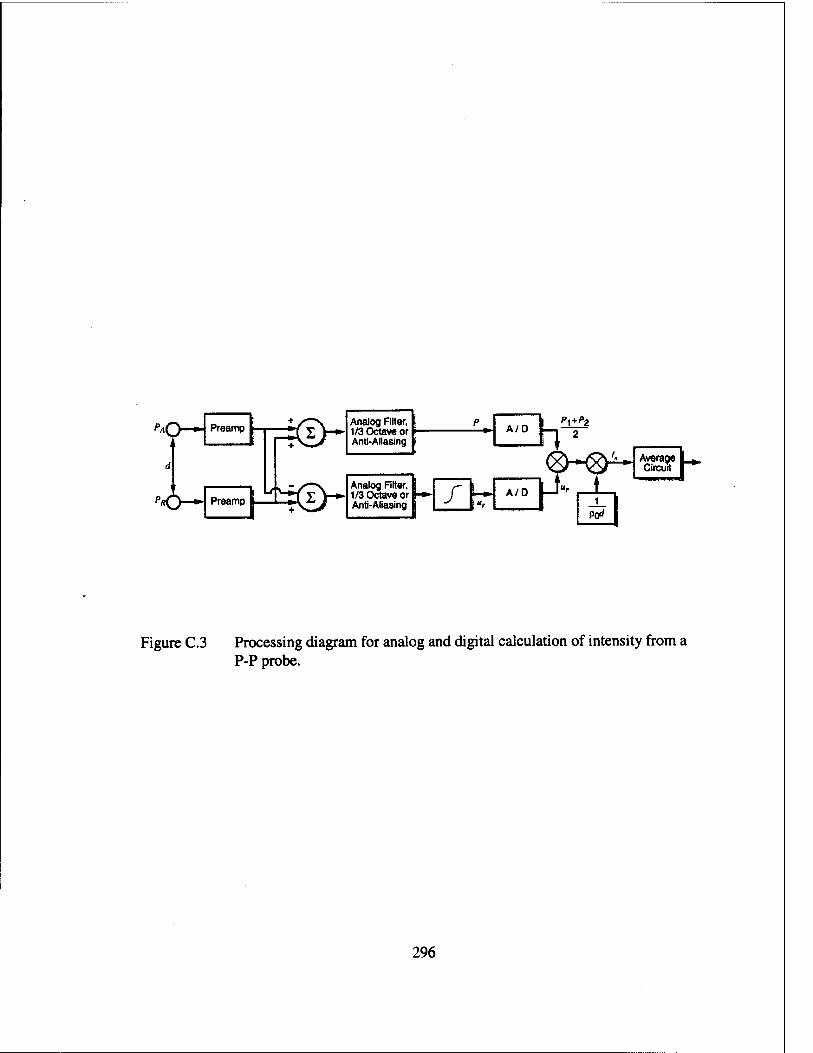
PAQ Preamp
J
pO
F=©~
Preamp P^>*
Analog Filter, 1/3 Octave or Anti-Aliasing
P A/O 1 i I
Analog Filter, 1/3 Octave or Anti-Aliasing f 40 [
Figure C.3 Processing diagram for analog and digital calculation of intensity from a P-P probe.
296
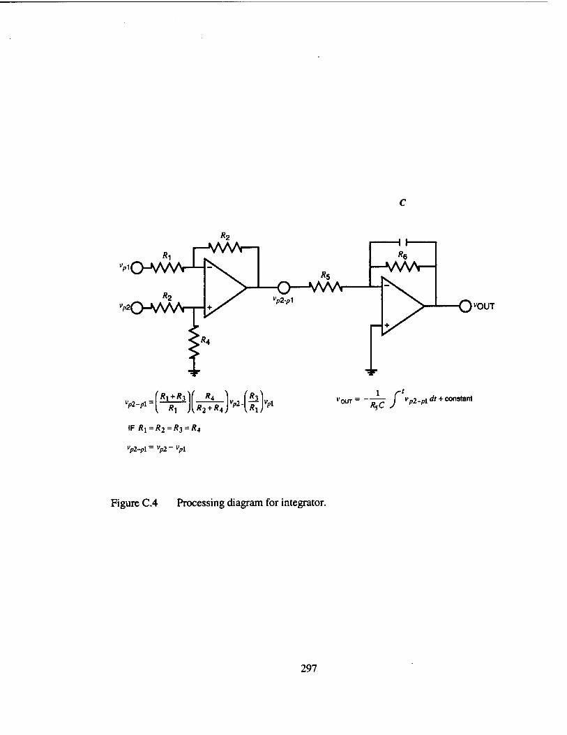
R2
*5
O—WA O^UT
v-^l^K^jv-^jv 'OUT -*c/^*+ constant
"p2-pl = ^2 - "pi
Figure C.4 Processing diagram for integrator.
297
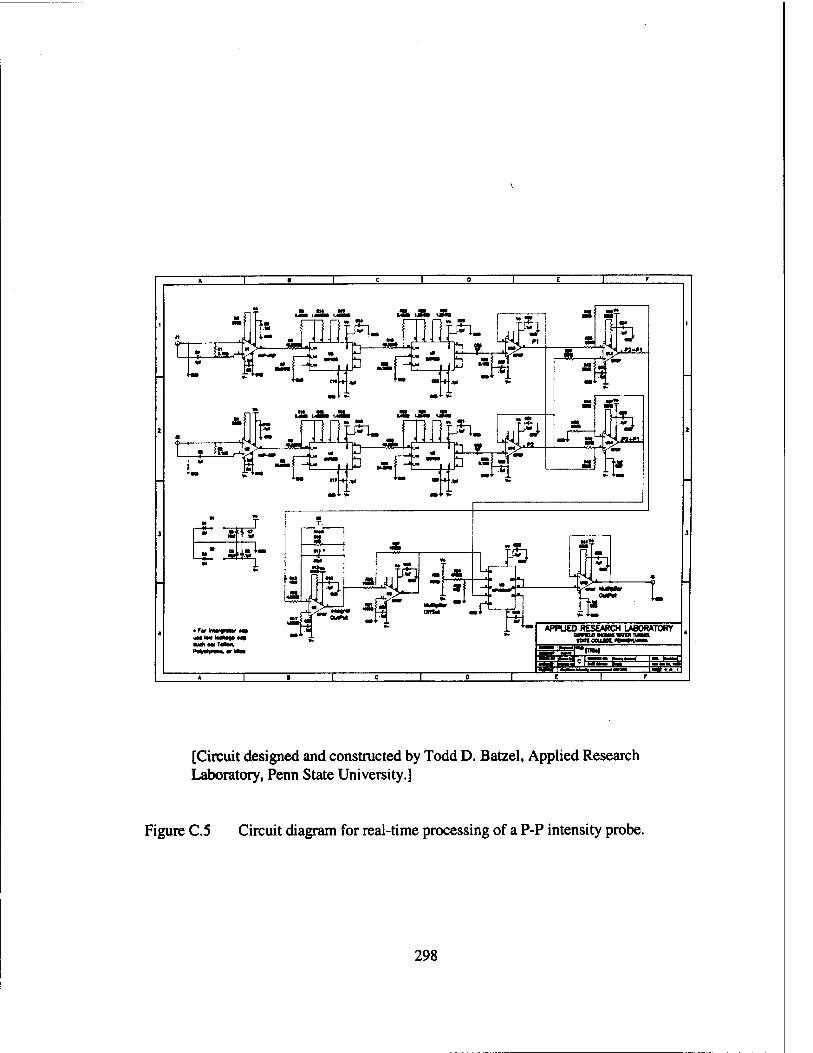
Äu&.,a. AA&
«7L -SU-
^1 13 ^
[>
-:-ja *J
1 APPUED RESEARCH LABORATORY
*n«M
s^a^fss^a
[Circuit designed and constructed by Todd D. Batzel, Applied Research Laboratory, Penn State University.]
Figure C.5 Circuit diagram for real-time processing of a P-P intensity probe.
298
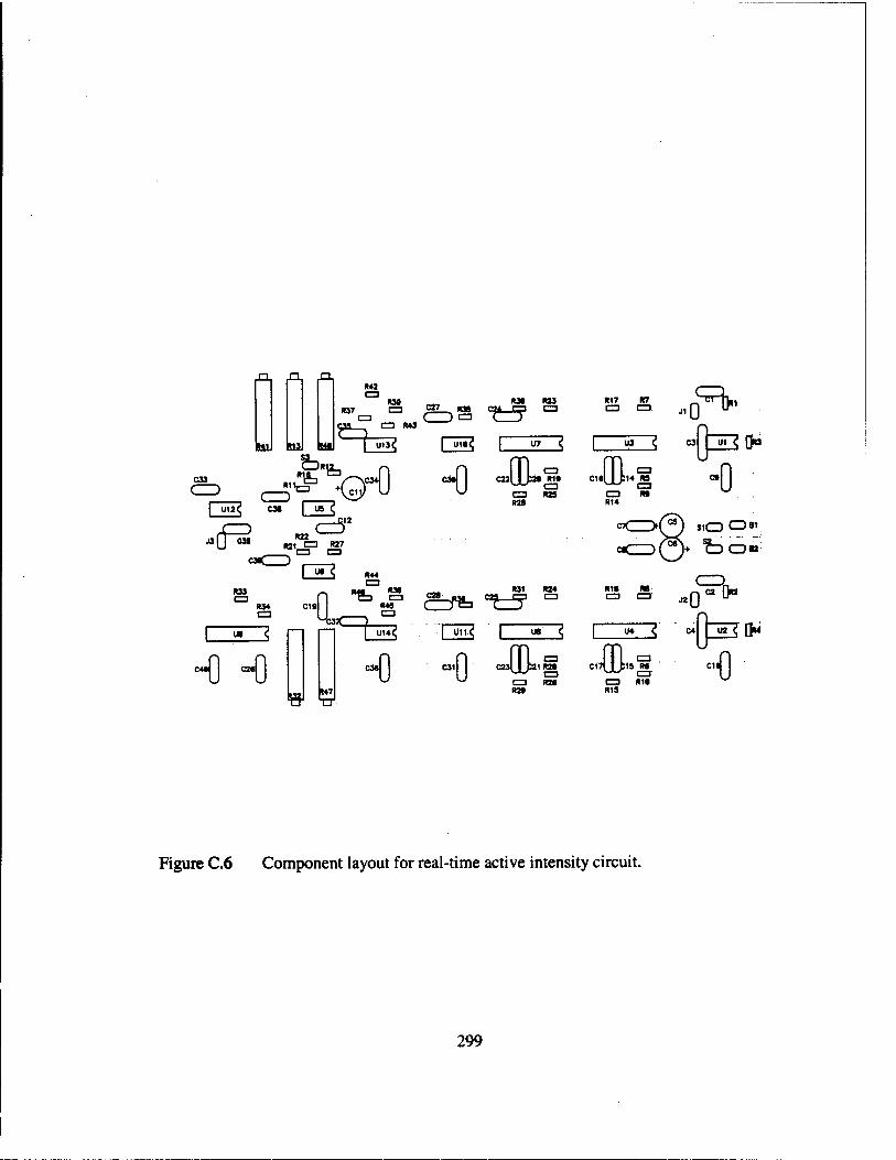
XX XX
fciiJ km
R4J FO» tat tos
C3 MS
I "'»< I "7 <
&R&
RII^J3
Ull^ CM | US <
C3 R1»
C3 C3 WS
J3 y OM
R3S
R22
I "» < R44
KS* CIS
•0 ~0 w
^ I U14< - ' | -U11.< I W <
«47
csd <si aaLD31 RM
R2t
R17 R7 -TBMIW
i « < «rprsöo
en|iJ»4g "U " C3 Rt . . R14
a s „Q^
i—^ a«* ^^
Figure C.6 Component layout for real-time active intensity circuit.
299
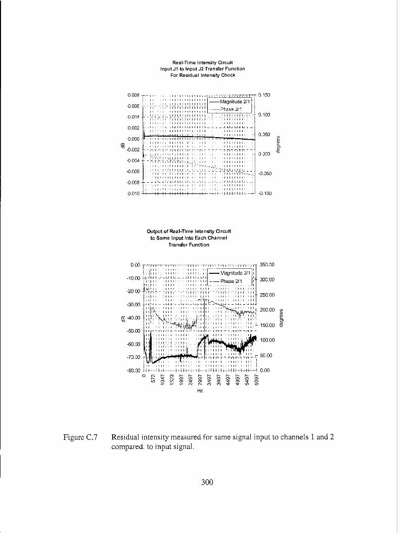
Real-Time Intensity Circuit Input J1 to Input J2 Transfer Function
For Residual Intensity Check
0.008
0.006
0.004
0.002
0.000
' -0.002
-0.004
-0.006
-0.008
-0.010
I I I I i I I I I I I I I II II ' I I ! ! I I i i
MMM M MM M M MM M M !
11 1 M 1 It 1 1 1 1 1 1 11 M
Magnitude 2/1
-—Phase 2/1 II M M M M ! M ! M M M ! ! ! ! ! II 1 1 M II M M II M II M II M 1 IIIMIIIIIIIIIIII r -
.UJUlUiULlJLULIIUlUiULIJ LIlLllLllUiU. ill 1 1 [ M M 1 1 1 M 1 M >■ M M M 1 M M 1 M II M II I 1 i M 1 I 1 1 '»!-< Uli 1 M M i M M M M M 1 M 1 M ~
1 II M M M 1 M M M M M M M i M M I M M II II M II II - -IT n Tin T n rn rri rrruriTn m rn ni TIT n r n ■
M M T 1 1 T M M 1 (T-i-'-U J 1 1 1 M II 1 M II M II M M 11 1 1 M i i : M t : i M i it i ! i i i rn-;<uj i i i i i M M I M I I I I
1 M II 1 M 1 M 1 M M M M iTrrT+JJJ_M
M i MM f - M M 1 1 M II 1 II M II M 1 1 1 1 1 i M M 1 1 1 t 1 1 1
M I M '. M 1 M 1 M 1 M ! 1 ! M II 1 1 ! M M M M M It 1 1 II i ll ■ ! : - i 1 . M l M M ' . M M M ! 1 1 M 1 i M 1 M 1 M M M
- I 1 [ ' 1 ! ' 1 1-1 1 1 ! 11 I 11 1 1 ! 1 1 1 1 1 1 it 1 1 1 i 1 i 1 1 i 1 1 1 i ! 1
0.150
0.100
- 0.050
- 0.000
■M- -0.050
-0.100
Output of Real-Time Intensity Circuit to Same Input into Each Channel
Transfer Function
T-T-x-cNjc\icoco-3--*mm
Hz
Figure C.7 Residual intensity measured for same signal input to channels 1 and 2 compared, to input signal.
300
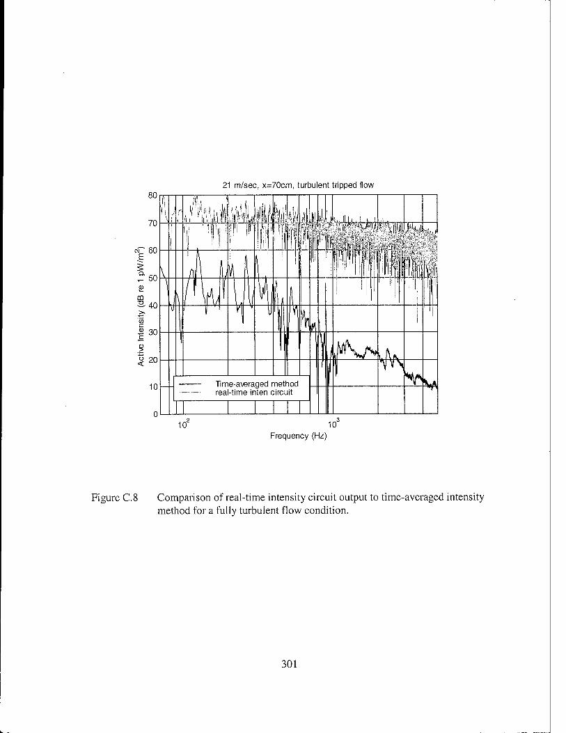
21 m/sec, x=70cm, turbulent tripped flow
Frequency (Hz)
Figure C.8 Comparison of real-time intensity circuit output to time-averaged intensity method for a fully turbulent flow condition.
301
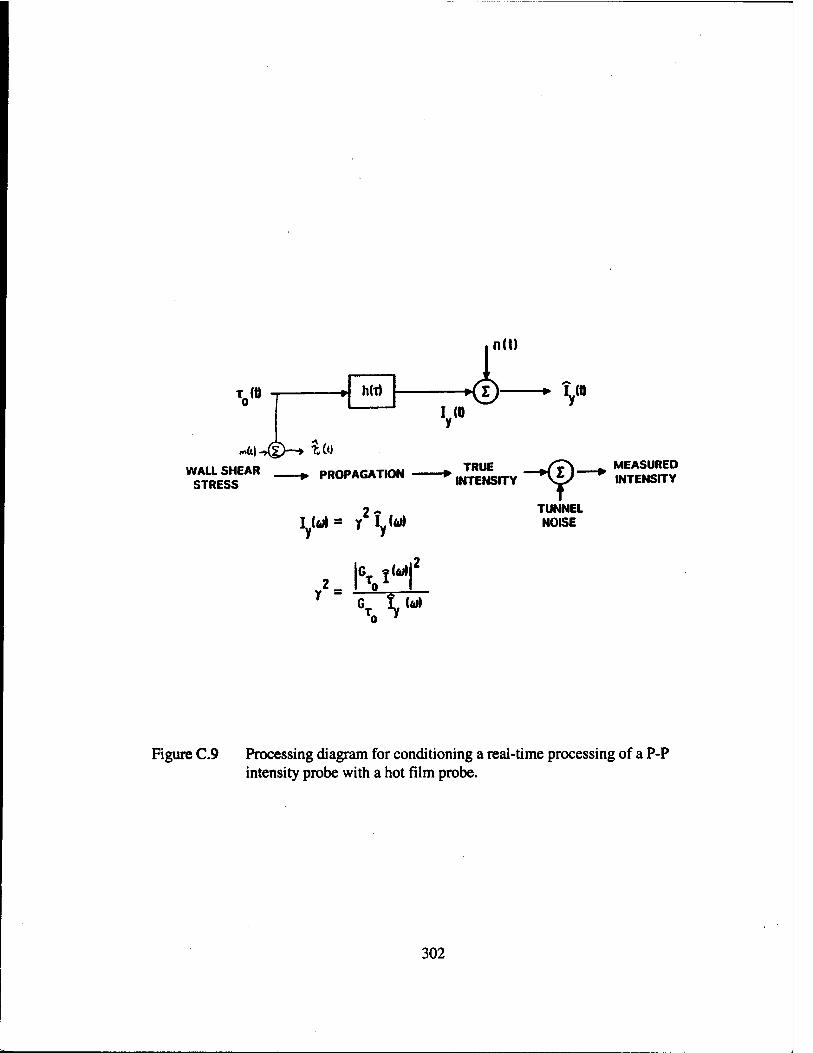
Vö hW
,n(t)
-*©—-\ (0
*&)->(!>-♦ iw TRUE -©• WALL SHEAR PROPAGATION ► .NTCMSITV
STRESS INTENSITY >^
2 ~ TUNNEL ilwi = r y** NOISE
MEASURED INTENSITY
2_ I -o y =
2 Ml' G_ ?(«)
0 7
Figure C.9 Processing diagram for conditioning a real-time processing of a P-P intensity probe with a hot film probe.
302
VITA RICHARD CHOSTNER MARBOE
Richard C. Marboe was born June 2,1959 in Spring Township, Pennsylvania. He graduated from State College Area High School in June, 1977. He received his SB in Mechanical Engineering and SM in Ocean Engineering from the Massachusetts Institute of Technology in June, 1982. He joined the research faculty at the Applied Research Laboratory at Penn State after five years as a submarine and engineering duty officer in the US Navy. His ARL management positions have included Program Manager in the Submarine & Ship Technology Office, Deputy Head of the Row and Structural Acoustics Department, and leader of the Flow Acoustics and the Research Facilitation Groups within that department. His Navy sponsored research has spanned leading propulsor design programs for submarine, surface ship, and weapon propulsors, two-phase flow acoustics (cavitation, bubble excitation, acoustic propagation screening), and hull flow- induced noise. He is a member of the American Society of Mechanical Engineers (Chair of the Turbomachinery Vibration and Noise Technical Comm.) and the Acoustical Society of America. He is the author of several scientific journal and symposia articles and over 35 ARL technical reports.