1

Limitation of atmospheric composition

by combustion-explosion in exoplanetary atmospheres

Grenfell, J. L.1#, Gebauer, S.1, Godolt, M.2, Stracke, B.1, Lehmann, R.3, and Rauer, H.1,2

1 Abteilung Extrasolare Planeten und Atmosphären (EPA), Institut für Planetenforschung (IP),

Deutsches Zentrum für Luft- und Raumfahrt (DLR), Rutherford Str. 2, 12489 Berlin, Germany

2 Zentrum für Astronomie und Astrophysik (ZAA), Technische Universität Berlin (TUB), Hardenbergstr. 36, 10623 Berlin, Germany

3 Alfred-Wegener-Institut, Helmholtz-Zentrum für Polar- und Meeresforschung,

Telegrafenberg A43, 14473 Potsdam, Germany

#Corresponding author, contact details:

Email: lee.grenfell@dlr.de

Tel: +49 30 67055 7934

FAX: +49 30 67055 384

Manuscript accepted for ApJ February 2018

2

Abstract: This work presents theoretical studies which combine aspects of combustion and explosion

theory with exoplanetary atmospheric science. Super-Earths could possess a large amount of molecular

hydrogen depending on disk, planetary and stellar properties. Super-Earths orbiting pre-main sequence-

M-dwarf stars have been suggested to possess large amounts of O2(g) produced abiotically via water

photolysis followed by hydrogen escape . If these two constituents were present simultaneously, such

large amounts of H2(g) and O2(g) can react via photochemistry to form up to ~10 Earth oceans. In cases

where photochemical removal is slow so that O2(g) can indeed build-up abiotically, the atmosphere

could reach the combustion-explosion limit. Then, H2(g) and O2(g) react extremely quickly to form water

together with modest amounts of hydrogen peroxide. These processes set constraints for H2(g), O2(g)

atmospheric compositions in Super-Earth atmospheres. Our initial study of the gas-phase oxidation

pathways for modest conditions (Earth’s insolation and ~ a tenth of a percent of H2(g)) suggests that

H2(g) is oxidized by O2(g) into H2O(g) mostly via HOx and mixed HOx-NOx catalyzed cycles. Regarding

other atmospheric species-pairs we find that (CO-O2) could attain explosive-combustive levels on mini

gas planets for mid-range C/O in the equilibrium chemistry regime (p>~1bar). Regarding (CH4-O2), a

small number of modeled rocky planets assuming Earth-like atmospheres orbiting cooler stars could have

compositions at or near the explosive-combustive level although more work is required to investigate this

issue.

Key words: Exoplanets, atmospheres, combustion, explosion

3

1. Introduction and Motivation

The atmospheres of Super-Earths (SEs) orbiting M-dwarf stars could build-up large amounts of

abiotically-produced oxygen (O2) via photolyis of water followed by escape of atomic hydrogen during

the pre-main sequence phase (Luger and Barnes, 2015). Planetary formation studies (e.g. Chian and

Laughlin, 2013) suggest that SEs could retain large amounts of molecular hydrogen (H2) from the

protoplanetary disk. The current work proposes that Combustion-Explosion (CE) reactions (e.g. Cohen,

1992) could limit the composition of exoplanetary atmospheres depending on pressure (p) and

temperature (T) if a fuel gas (such as molecular hydrogen, H2) is present together with an oxidant gas

(such as molecular oxygen, O2) initiated by lightning or cosmic rays. Whether SEs could reach the CE limit

depends on the planetary evolution, specifically the timescales for photochemical oxidation, escape etc.

which impact the abundance of potential combustants such as H2(g) and O2(g).

Water delivery and migration of SEs orbiting in the HZ is rather contested (Raymond et al., 2007,

Ogihara and Ida, 2009). For SEs in the Habitable Zone (HZ) of M-dwarf stars explosion-combustion could

represent an important mechanism by reaction of H2(g) and O2(g) for generating oceans. These would

likely however contain some hydrogen peroxide (H2O2) (see CE mechanism in section 4.1) which is

unsuitable for life as we know it. Also, gaseous mixtures containing (CO-CH4-O2-N2) could possibly

explode or combust on some Mini Gas Planets (MGPs) (see section 7) and on some Earth-like worlds

orbiting cooler M-stars if methane builds up to above ~(2-3)% by volume (see section 8).

Section 2 considers chemical disequilibrium, combustion and life and evidence for combustion

of O2(g) in early Earth’s atmosphere. Section 3 discusses the initiation of CE by lightning and cosmic rays

in (exo)planetary atmospheres. Section 4 reviews CE processes for (H2-O2) atmospheres. Sections 5 and

6 present the run scenario and results respectively from a model study of [H2-O2] atmospheres. Sections

7, 8 and 9 discuss potential CE for (CO-O2), (Hydrocarbon-O2) and (NH3-containing) gas mixtures

respectively. Section 10 briefly discusses explosions related to atmospheric dust suspensions. Section 11

presents a brief discussion and conclusions.

2. Chemical disequilibrium, (atmospheric) combustion and life

Is it possible that only planets with life could produce sufficient chemical disequilibrium to

generate combustion, as occurred on the early Earth? Simoncini et al. (2013) calculated that 0.67

terawatts (TW) are required to maintain the (CH4(g)-O2(g)) redox disequilibrium in modern Earth’s

atmosphere with 0.24 TW associated with abiotic geological processes. They noted that this value is

negligible compared with the modern Earth’s total incoming solar energy (175,000 TW) and very low

4

compared with our planet’s total photosynthetic productivity (215 TW). The low redox disequilibrium

value (=0.24 TW) is however likely to be broadly comparable with the energy associated with

geochemical surface processes e.g. the dissolution of crust via precipitation on the modern Earth.

Krissansen-Totton et al. (2016) compared atmospheric chemical redox disequilibria for Earth and other

Solar System bodies and suggested that the large abundance of (N2(g)-O2(g)) in Earth’s atmosphere

together with the presence of global-scale oceans constitutes a significant source of thermodynamic

disequilibrium. In general, there exists a wide range of abiotic processes known to generate redox

disequilibrium - but their extent and magnitude on global scales compared with those due to life is not

well-determined. Could, for example, the modern Earth’s (CH4(g)-O2(g)) redox disequilibrium be

produced abiotically? Today, up to 10% (equivalent to a few tens of Tg/yr) of total CH4(g) emitted on

Earth’s surface is produced geothermally and the rest arises mainly via biology. On the early Earth,

however, geothermal outgassing from CH4(g) via mid-ocean ridges could have been significantly

enhanced (Pavlov et al., 2000) compared with today. Also, regarding O2(g), recent advances (see above)

suggest that abiotic sources may have been strongly under-estimated depending on the planetary

environment (instellation etc.). It seems therefore at least conceivable, that abiotic processes under

certain circumstances could rival redox disequilibrium from biology.

2.1 O2 combustion in Early Earth’s atmosphere

Surface O2 in early Earth’s atmosphere reached a maximum abundance of ~0.3 bar during the

Carboniferous period about (300-400) Myr ago likely via increased organic burial associated with

widespread vascular land plant coverage (Dahl et al., 2010). Higher O2 abundances were prevented

however, likely due to O2 combustion of organic carbon to form CO2 as suggested by studies of

fossilized-charcoal from paleofires initiated by lightning (Heath et al., 1999; Berner, 1999). Clearly there

are differences between the case of early Earth (where large atmospheric oxygen abundances are driven

mainly by life and where it is organic material which combusts) - compared with the proposed Super-

Earth cases (where atmospheric oxygen is abiotically-formed and combustion takes place via the gas-

phase oxidation of H2(g)) . Nevertheless the case of early Earth is mentioned here as an example where

O2(g) is limited by combustion during a planet’s evolution.

Although it may seem at first counter-intuitive, CE events early in a planet’s history could in

some ways favor the development of life e.g. firstly by helping to maintain oceans over longer

timescales. Secondly, in (O2-N2) atmospheres combustion can form nitrogen oxides i.e. a form of fixed

5

nitrogen useful for life. In (O2-CO2-N2) atmospheres combustion can form hydrogen cyanide (HCN)

(Giménez-López et al., 2010) which is a well-known precursor of amino acids (e.g. Yuasa et al., 1984).

3. Initiation of Combustion-Explosion in Planetary Atmospheres

Combustion and/or Explosion can be initiated when stable compounds such as molecular

hydrogen are split by input of energy from lightning or/and cosmic rays to form reactive radicals. The

resulting atoms can go on to initiate radical chain reactions which release energy faster than it can be

removed by the surroundings.

3.1 Lightning

Similar to the way that an electric spark can be used in the laboratory to initiate combustion-

explosion, lightning (and cosmic rays) represent natural phenomena which can also lead to these

processes. An average single lightning flash delivers ~6x109 Joules on the modern Earth (Hill, 1991) and -

analogous to an electrically-generated spark - leads to electrostatic discharge in the Earth’s atmosphere.

Modern Earth features on average ~44 lightning flashes s-1 (intra-cloud and cloud-to-ground

combined) with generally more activity over land and in the tropics (Christian et al., 2003; Oliver, 2005).

Earth's lightning activity breaks molecular nitrogen into atomic nitrogen – this reacts with oxygen

compounds to likely produce (2-10)Tg (N)/year of nitrogen oxides (NOx) which can catalytically remove

ozone in the stratosphere (e.g. Pickering et al., 1998).

On the early Earth, global lightning activity is not well constrained (Navarro-González et al.,

1998; Navarro-González et al., 2001). Volcanic lightning was likely enhanced and thunderstorm lightning

may also have been stronger due to possibly enhanced atmospheric dynamics due to a closer Moon and

a faster rotating planet - although more work to study such effects is required.

On Venus, lightning activity is estimated to be about 20% that of modern Earth (Russell et al.,

2008) although optical evidence is still rather lacking (Cardesίn-Moinelo et al., 2016; Yair, 2012). On

Mars, electrical discharge is thought to occur frequently in dust devils and synoptic to global-scale dust

storms (Yair, 2012 and references therein). On Jupiter and Saturn, integrated occurrence rates of

lightning are estimated to be about one hundred times that of modern Earth and peak in the water

cloud layers at 5 bar and 10 bar respectively (Yair, 2012 and references therein).

In summary, lightning is widespread in planetary atmospheres in the solar system. For SEs

orbiting in the HZ of an M-dwarf star, General Circulation Model (GCM) studies (e.g. Joshi et al., 1997;

Kite et al., 2011; Yang et al., 2013; Mills and Abbot, 2013) have suggested strong day-to-night circulation

6

to maintain habitability which may provide wind velocities sufficient for charge separation hence favor

the onset of lightning.

3.2 Cosmic Rays

Stellar (and Galactic) Cosmic Rays (CRs) can penetrate deeply into Earth’s atmosphere (e.g.

Veronnen et al., 2008). For SEs orbiting in the HZ of an active M-dwarf star, high inputs of Stellar and

Galactic CRs could be present due to strong stellar activity, the close proximity to the star and the

potentially weakened planetary magnetosphere associated with tidal-locking (e.g. Grieβmeier et al.,

2005; Grenfell et al., 2007; Grenfell et al., 2012). Galactic Cosmic Rays with energies around the knee

region of the energy spectrum and above i.e. >1016 eV (about 1.6 mJ) could initiate (depending on

atmospheric composition, T, p etc.) combustion. These have an occurrence rate near modern Earth’s

surface of several particles m-2 year-1. By comparison the “Minimum Ignition Energy” per spark to initiate

combustion is ~0.03mJ (for H2 in air), ~1mJ (for hydrocarbons in air) and ~1J for dust explosions in air

(see also section 9) (Lackner, 2009).

4. Combustive-Explosive Gas Mixtures of (H2-O2)

Rapid release of energy can occur in gas mixtures when runaway chemical production (chain

propagation) of free radicals occurs faster than the corresponding sink (termination) reactions which

remove the free radicals. Depending on p, T there are in general two main mechanisms for energy

release, namely via explosion (detonation) in which a pressure wave moves supersonically away from

the ignition site and combustion (deflagration) in which a sub-sonic pressure wave together with

electromagnetic radiation are generated. Combustion can occur either via energy input via sparks

created when an applied electric field leads to dielectric breakdown of the gas molecules. Alternatively,

combustion can occur via lightning or/and cosmic rays which can also lead to splitting or/and ionization

of air molecules, or can be spontaneous, referred to as ‘self-combustion’. The energy required to induce

CE is termed the “minimum ignition energy” and is usually expressed in Joules.

Distinguishing between whether a given gas mixture explodes or combusts over a range of (p-T)

is observationally challenging due to the power and complexity of the reaction mechanisms (see e.g.

Sichel et al., 2002). Therefore in this work we use where possible the term “combustion-explosion (CE)”

together. We now discuss CE for different gas-mixtures and place them in the context of exoplanetary

atmospheres.

7

4.1 Mechanism for [H2-O2] Combustion-Explosion

Mixtures of H2-O2 gas, denoted as “oxyhydrogen”, “electrolytic gas” or “detonating gas” are

known to react either explosively or to combust, producing energy and the stable product water (H2O).

Assuming complete oxidation of H2 by O2, the overall (net) reaction is: H2+½O2 H2O. However, in

practice the mechanism consists of intermediate steps in which other stable reaction products such as

H2O2 can form. The key reaction steps of the H2-O2 CE mechanism (e.g. Cohen, 1992) are as follows:

H2 H + H (1) H + O2 OH + O (2) O + H2 OH + H (3) OH + H2 H + H2O (4) H + H + M H2 + M (5) O# + O + M O2 + M ` (6) O + H + M OH + M (7) H + OH + M H2O + M (8) H + O2 + M HO2 + M (9) HO2 + H2 H2O2 + H (10) H/O/OH/HO2 + surface## products (11) [#O-atoms supplied into the system via e.g. CO2 photolysis; ## removed from the system via gas-surface heterogeneous reactions occurring on the reaction chamber vessel or, in the case of a planetary atmosphere on the surface (if present) or on atmospheric aerosol]. Reaction (1) is the initiation step in which H2 is dissociated in planetary atmospheres by lightning

or by cosmic rays. H2 has a minimum ignition energy in the range 0.02mJ/spark (US Dept. of Energy,

Hydrogen Fact Sheet 1.008) to 0.03 mJ/spark (Lackner, 2009). This compares with a value of 0.29mJ for

CH4, with values generally >0.2mJ for higher hydrocarbons (Ono and Oda, 2008) and with values of

typically ~1000mJ for dusts (many solids become very flammable when reduced to a fine powder in air).

In general these energies depend on the gas composition, the total pressure and the spark duration

(Maas and Warnatz, 1988; Ono and Oda, 2008). Note that the symbol ‘M’ in reactions (5) to (9) above

refers to any third body present in the gas-phase required to remove excess vibrational energy of the

reactants. Reactions (1-10) are commonly implemented in photochemical models in the literature.

Required in order to simulate CE if it occurs are (i) the chemical heats of reaction which drive the rapid

and runaway energy release, or/and (ii) treatment of cosmic rays which convert molecular into atomic

hydrogen, or/and (iii) the energy budget via thermal diffusion, conduction etc. (see next section).

Reactions (2)-(4) are the propagation steps. Reactions (2) and (3) are called “chain branching” since they

produce two reactive products namely (OH,O) and (OH,H) respectively from one radical reactant and

can therefore lead to runaway propagation (production) of radicals. Reactions (5)-(9) represent the

termination steps which overall remove chain carriers. Reaction (11) denotes sticky collisions of gas

8

species with solid surfaces. Appendix one suggests that the importance of heterogeneous chemistry in

removing reactive gas-phase species (reaction 11) is less for planetary atmospheres than for reaction

vessels. This suggests that CE could be reached for a wider [p,T,composition] range in planetary

atmospheres compared with reaction vessels.

Rapid release of energy occurs when the runaway propagation steps start to rapidly exceed the

termination steps. Note that the mechanism produces H2O (reaction 8) and H2O2 (reaction 10) as stable

products. With the addition of N2(g) i.e. on considering (H2-O2-N2) mixtures, there occur mixed nitrogen-

oxygen reactions:

O + N2 NO + N (12) N + O2 NO + O (13) N + OH NO + H (14) Reactions 12 and 13 are collectively referred to as the Zeldovich mechanism (Zeldovich, 1947).

4.2 Evolution of atmospheric [H2:O2] in Super-Earths

Figure 1 summarizes processes affecting H2(g) and O2(g) in SE atmospheres:

Figure 1: Processes affecting H2(g) and O2(g) in SE atmospheres.

In Figure 1, H-atoms from H2O photolysis can escape, especially during the active pre-main

sequence phase of the star and can even drag off heavier O atoms during this stage. The remaining O-

9

atoms (which can also be formed via CO2 photolysis) can combine with themselves in a three-body gas-

phase reaction to form O2(g) abiotically. H2(g) and O2(g) can either undergo CE if suitable conditions of

[p,T, composition] are achieved to form water plus energy, or they can react via photochemistry. The

amount of H2 retained from the protoplanetrary disk therefore depends sensitively on the planet’s

mass, the size of the disk and the insolation from the star (Lammer et al., 2014; Luger et al., 2015) and

can cover a wide range - from complete loss of H2 up to about one percent H2 of the total planetary mass

(See also references in Table 1 below).

The amount of (abiotic) O2 in the SE atmosphere is also predicted to cover a wide range

depending on the UV from the central star and on model treatments of photolysis and atmospheric

escape. Abiotic O2 production proceeds e.g. via either carbon dioxide (CO2) photolysis followed by

recombination of oxygen (O) atoms with each other (e.g. Canuto et al., 1982) or, via water H2O

photolysis followed by escape of atomic hydrogen (H) (Berkner and Marshall, 1964). The modern Earth

features a column O2 value of 4.5x1024 molecules cm-2 (Schneising et al., 2008). Segura et al. (2007)

(their Table 2) however suggested abiotic O2 amounts for CO2-dominated atmospheres in the range

(2x1018-8x1019) molecules cm-2 (depending on the assumed outgassing rates, photochemical reaction

rates, incoming UV etc.) i.e. up to about six orders of magnitude smaller than the modern Earth. Their

study included rainout of oxidized species which led to a high abundance of reducing species (like H2)

hence their column O2 values remained low. Model studies by Hu et al. (2012) (their Table 7) and Tian et

al. (2014) (their Figure 3) - which included redox balance and thermal escape - suggested stronger

abiotic O2 amounts than the Segura study, i.e. about 100 times smaller than on modern Earth. Hu et al.

(2012) calculated a mean mixing ratio over the atmospheric column of 1x3x10-3 O2 for a terrestrial

planet with a 90% CO2 atmosphere orbiting a Sun-like star. Tian et al. (2014) suggested that the

established OH-catalyzed cycles which drive the recombination of CO with O into CO2 would be slow on

SEs orbiting M-dwarf stars (i.e. favoring O2 abiotic production up to 1000 times greater than for Sun-like

stars) due to the weak Near-UV (NUV) output from the central star since NUV leads to release of

atmospheric OH from its reservoirs (see also Harman et al., 2015). The model study by Domagal-

Goldman et al. (2014) included redox balance of both the atmosphere and the ocean system and

calculated modest abiotic O2 columns of (3x1019-2x1021) molecules cm-2 depending on stellar type,

assuming atmospheres with 1bar surface pressure and CO2 volume mixing ratios of 0.5. They suggested

that model differences with the above-mentioned Hu and Tian studies could have arisen due to different

treatments of CO removal from the atmosphere. Harman et al. (2015) noted the importance of redox

balance in the atmosphere-ocean system and estimated an abiotic O2 column of 9.3x1022 molecules cm-2

10

(i.e. ~2% of modern Earth) for an Earth-like planet with a 5%CO2 atmosphere orbiting in the HZ of GJ876

(an M4V star). Wordsworth and Pierrehumbert (2014) suggested that planets with low abundances of

non-condensing gases such as molecular nitrogen (N2) would feature weak cold traps hence rapid H2O

photolysis which could lead to efficient abiotic O2 production. The presence of a large H2(g) atmosphere

could therefore weaken or halt this mechanism although the location and magnitude of the cold trap in

such atmospheres requires further investigation. Luger and Barnes (2015) modeled early stages of

planets orbiting cooler stars (without large H2(g) envelopes) and suggested very large abiotic O2 with up

to two thousand times the mass of Earth’s atmospheric O2. In their study abiotic production is favored

by strong incoming X-ray Ultra Violet (XUV) radiation from young (up to 1Gyr) pre-main sequence M-

dwarf stars which drives fast photolysis of H2O and escape of the resulting H in the planetary

atmosphere. Regarding spectral features, Schwieterman et al. (2016)a,b discuss possible means of

identifying abiotic O2 spectral signals. Garcίa Muñoz et al. (2009) investigated spectroscopic features of

the O2 dimer nightglow. More work is required to constrain better the range of possible CO2 and H2O

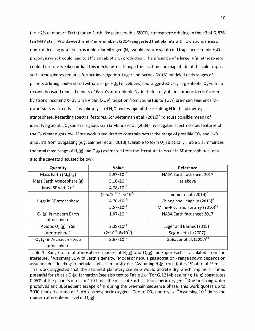
amounts from outgassing (e.g. Lammer et al., 2013) available to form O2 abiotically. Table 1 summarizes

the total mass range of H2(g) and O2(g) estimated from the literature to occur in SE atmospheres (note

also the caveats discussed below):

Quantity Value Reference Mass Earth (Me) (g) 5.97x1027 NASA Earth fact sheet 2017

Mass Earth Atmosphere (g) 5.10x1021 as above Mass SE with 2re

§ 4.78x1028

H2(g) in SE atmosphere (2.5x1019-1.5x1026)

4.78x1026 3.57x1023

Lammer et al. (2014)* Chiang and Laughlin (2013)#

Miller-Ricci and Fortney (2010)§§ O2 (g) in modern Earth

atmosphere 1.07x1021

NASA Earth fact sheet 2017

Abiotic O2 (g) in SE atmosphere#

2.38x1024

(2x1018-8x1019) Luger and Barnes (2015)**

Segura et al. (2007)+ O2 (g) in Archaean –type

atmosphere 5.67x1016 Gebauer et al. (2017)##

Table 1: Range of total atmospheric masses of H2(g) and O2(g) for Super-Earths calculated from the literature. §Assuming SE with Earth’s density. *Model of nebula gas accretion - range shown depends on assumed dust loadings of nebula, stellar luminosity etc. #Assuming H2(g) constitutes 1% of total SE mass. This work suggested that the assumed planetary scenario would accrete dry which implies a limited potential for abiotic O2(g) formation (see also text to Table 1). $$For GJ1214b assuming H2(g) constitutes 0.05% of the planet’s mass, or ~70 times the mass of Earth’s atmospheric oxygen. **Due to strong water photolysis and subsequent escape of H during the pre-main sequence phase. This work quotes up to 2000 times the mass of Earth’s atmospheric oxygen. +Due to CO2-photolysis. ##Assuming 10-5 times the modern atmospheric level of O2(g).

11

In Table 1, the H2(g) mass range varies from ~(1019-1026)g whereas O2(g) varies from ~(1016-

1024g). Estimating however which combinations of H2(g) and O2(g) could actually co-exist in SEs in

nature, requires further studies with coupled chemistry-climate models which calculate consistent, gas-

phase chemical evolution. Note that the extent to which SEs in the HZ of low mass stars accrete water

during their formation (hence their ability to form O2(g) abiotically via water photolysis followed by H-

escape) is a subject of discussion (see e.g. Lissauer, 2007; Hansen, 2015). Recent model studies

addressing abiotic O2(g) formation (e.g. Hu et al., 2012; Tian et al., 2014; Harman et al., 2015) all assume

low reducing conditions with relatively small H2(g) abundances. It is challenging for current coupled

climate-photochemistry models to operate over such large p, T and composition ranges including all

relevant processes (climate, chemistry, escape etc.) Notable model studies in this direction, however

are e.g. Miller-Ricci and Fortney (2010); Miguel and Kaltenegger (2013); Seager et al., (2013) and Hu and

Seager (2014). Similarly it is challenging to simulate thick steam atmospheres associated with the

strongest abiotic O2(g) production scenarios. The potentially large range of abiotic sources of O2(g)

shown in Table 1 are often-quoted in the exoplanetary community often without reference to

photochemical sinks of O2(g) due to large H2(g) envelopes which could be present in SEs.

Figures 2a-c show schematically examples of the evolution of key chemical species in SE

atmospheres for fast (molecular) hydrogen loss (Figure 2a), medium hydrogen loss (Figure 2b) and slow

hydrogen loss (Figure 2c):

Figure 2: Schematic evolutionary pathways of key chemical species in SE atmospheres for three hypothetical cases, namely fast H2 loss (Figure 2a, left panel), medium H2 loss (Figure 2b, middle panel) and slow H2 loss (Figure 2c, right panel). Hydrogen loss can be driven by either strong incoming EUV or a large amount of hydrogen initially accreted. The shaded rectangular region in Figure 2b shows species’ response to possible combustion-explosion. Species shown are: H2 (solid black line), H2O (dashed black line), O2 (dotted black line) and H2O2 (dotted grey line).

Atm

osph

eric

Abu

ndan

ce

(arb

itrar

y un

its)

Time (arbitrary units)

H2

O2

H2O

Atm

osph

eric

Abu

ndan

ce

(arb

itrar

y un

its)

Time (arbitrary units)

H2

O2

H2O

H2O2

Atm

osph

eric

Abu

ndan

ce

(arb

itrar

y un

its)

Time (arbitrary units)

H2

O2

H2O

H2O2

Figure 2a: Fast H2 loss

Figure 2b: Medium H2 loss

Figure 2c: Slow H2 loss

HYDROGEN STARVED:

NO EXPLOSION EXPLOSION-

COMBUSTION

OXYGEN STARVED:

NO EXPLOSION

12

The three panels in Figure 2 describe hydrogen loss as well as oxygen and water formation

under different EUV conditions. Hydrogen loss depends on e.g. the initial amount of H2 accreted from

the protoplanetary disc and upon the escape rate of hydrogen atoms. This escape is essentially driven by

EUV insolation and can proceed in two steps – first via photochemical release of hydrogen atoms from

hydrogen-containing molecules (e.g. H2O, CH4, H2 etc.) (which takes place in the middle atmosphere and

above) and second via diffusion- or/and energy-limited escape. Oxygen (abiotic) formation proceeds via

gas-phase combination of O-atoms which originate from water photolysis or from photolysis of other O-

containing species such as CO2.

Figure 2a shows the “H2-starved case” i.e. where the CE limit is not reached because hydrogen

loss is rapid (associated with strong incoming EUV) so that its abundance drops below the CE limit

before O2 can sufficiently build-up. Figure 2b shows the case where hydrogen is lost more slowly than in

Figure 2a hence the system remains above the CE H2-lower limit for longer which means more time for

build-up of abiotic O2. Then, the CE limit can be reached as denoted by the grey-shaded rectangle. This

results in rapid ocean formation after a phase of ocean loss via evaporation and photolytic dissociation

of water. In Figure 2b assumes that the water reservoir is never larger than the initial inventory. In

addition to forming H2O, CE in Figure 2b leads to formation of some H2O2 which is gradually lowered e.g.

associated with the photolytic loss of H2O. Figure 2c shows the “O2-starved case” i.e. where the CE limit

is now not reached because weak incoming EUV leads to insufficient build-up of O2.

The effects of (classical, gas-phase) photochemistry should also be considered in Figure 2 in

addition to CE. For example, high H2 and high EUV could lead to faster photochemical removal of O2 by

H2 which could prevent O2 from reaching the CE limit. These effects should be the focus of future work

which requires a wider parameter range of study than possible in the present work.

4.3 Temperature-pressure dependence of [H2-O2] explosion

Figure 3 shows the characteristic S-curve for the [T-p] dependence of [H2-O2] explosion:

13

Figure 3: Temperature-pressure dependence of (H2-O2) explosion. Data source adapted from Lewis and von Elbe (1987) for a two-to-one hydrogen-to-oxygen stoichiometric mixture using a spherical vessel 7.4cm in diameter with a potassium chloride coating. The explosive region is shaded in grey, the non-explosive region is non-shaded. As an example at T=750K, the three points marked as “X” along the grey dashed line denote the first, second and third explosive limits i.e. where the grey-shaded and non-shaded regions cross. The red-pink shaded rectangle in the upper part of the Figure shows the relevant range (0.1-0.001bar) sampled via transit transmission spectroscopy (see e.g. Hu and Seager, 2014). Figure 3 shows the case for a 2:1 [H2:O2] stoichiometric mixture (although the CE limit can be

attained over a range of [H2:O2] mixtures depending on p, T, see Figure 4 below). Note too that for the

particular stoichiometric composition (H:O=2:1) assumed in Figure 3, CE proceeds for only ~T>660K.

Note that achieving the same stoichiometry as assumed in Figure 3 combined with these relatively high

middle atmosphere temperatures might therefore be limited to the early stages of a planet’s evolution if

the thick H2-dominated atmosphere is permanently lost thereafter. SEs however likely cover a wide

[p,T,composition] range as discussed below e.g. from potentially habitable conditions such as recently

suggested for Kepler 452b (Jenkins et al., 2015) to the hot, thin atmospheres of SEs such as CoRoT 7b

(Hatzes et al.,2011) where surface T at the sub-stellar point likely exceeds 2000K. The white (non-

explosive) and grey (explosive) regions in Figure 3 can be interpreted as follows:

0.001

0.01

0.1

1

10

600 700 800 900

Pres

sure

(bar

)

Temperature (K)

Non-Explosive

Region

x

x

x

Explosive Region

750K 850K

Hot Super-Earths second limit

third limit

first limit

14

At pressures lower than the first limit in Figure 3, the mixture is non-explosive (corresponding to

the unshaded region at the top of Figure 3) due to efficient diffusion favoring wall-reactions on the

reaction vessel (for an estimation of this effect for atmospheres, see appendix 1) which remove reactive

radicals. On increasing pressure, diffusion slows and the mixture becomes explosive i.e. the rate of the

propagation reactions exceed that of the termination reactions - at the ‘first (explosive) limit’. On

increasing pressure further, the mixture becomes once more non-explosive at the ‘second limit’ because

the pressure-dependent reaction 9 (whose rate varies approximately with p2) is now important in

removing H atoms; Lee and Hochgreb (1998) discuss effects affecting the second explosion limit and

present possible chemical pathways for H2 oxidation. At higher pressures still, reaction 10 can become

important in producing H and the mixture becomes once more explosive at the ‘third limit’. Schroeder

and Holtappels (2005) present the lower and upper explosion limits shown in the number of moles of H2

present as a % of the total moles (mol% H2) as a function of pressure. The lower limits vary from 4.3%

mol%H2 (1 bar) up to 5.6% mol%H2 (150bar); the upper limits vary from 76.5% mol%H2 (1 bar) (which

corresponds to a lower limit of 23.5%O2) down to 72.9% mol%H2 (150bar). Zheng et al. (2010) suggested

that experimental design (chamber size, shape, wall-coating etc.) leads to an error in the derived (p-T) of

both the lower and upper explosion limits by about 4%.

At temperatures above about 850K (see Figure 3) the system is explosive for all pressures. This is

because propagation reactions have generally moderately positive temperature-dependencies whereas

termination reactions have either only weakly positive or weakly negative temperature dependencies.

At intermediate temperatures (700-850K) the system can be explosive or not depending on the

pressure. Maas and Warnatz (1998) provide more details on the T-dependence of propagation and

termination reactions. Schroeder and Holtappels (2005) present the lower and upper explosion limits

(in mol%H2) as a function of temperature. The lower limits vary from 3.9% (293K) down to 1.5% (673K);

the upper limits vary from 75.2% (293K) up to 87.6% (673K).

4.4 Composition dependence of [H2-O2] combustion

Figure 4 shows the combustion (flammability) regions for (H2-O2-N2) and for (H2-O2-CO2) gas

mixtures at T=298K and p=1 bar:

15

Figure 4: Compositional dependence of the (H2-O2-N2) and (H2-O2-CO2) systems (shown in molar concentration by percent) upon combustion for gas mixtures at T=298K, p=1bar. The Figure shows %H2 concentration (y-axis) and %N2 (or %CO2) concentration (x-axis) with the remaining (“leftover gas”) being O2. In the shaded blue region both (H2-O2-N2) and (H2-O2-CO2) mixtures are flammable. In the shaded grey region both mixtures are non-flammable. In the central white region (H2-O2-CO2) mixtures are non-flammable whereas (H2-O2-N2) mixtures are flammable. The dashed grey line shows as an example the %molar gas composition of [60:16:24] for [H2:O2:N2]. Data shown is adopted from the same source as for Figure 3.

Figure 4 suggests that (H2-O2-N2) mixtures at T=298K and p=1bar are combustive (flammable) for

H2 concentrations of about (5-70%). Other studies (Schroeder and Holtappels, 2005) reported similar

limits at these (p,T) i.e. suggesting a lower limit of (3.6-4.2%)H2 and an upper limit of (75.1-77.0%).

Cohen (1992) on the other hand, (their Table 1 and references therein) suggested e.g. for O2/N2 of

(21:79) an %H2 lower limit from (4.2-9.4)% and upper limit from (64.8-74.7)%. In short, above about 70%

N2, the mixture in Figure 4 is non-combustive, whereas for high H2 concentrations this value decreases

to ~0% N2. On increasing the temperature for (H2-O2-N2) mixtures (e.g. to 300oC, not shown) the %

lower (upper) combustive limit for H2 concentration in Figure 4 is lowered (raised) by a few percent.

0

10

20

30

40

50

60

70

80

0 20 40 60 80

%Hy

drog

en (H

2)

%Nitrogen (N2) or Carbon dioxide (CO2)

(H2-O2-N2) and (H2-O2-CO2)

Flammable

24%

(22) (20) (18) (16) (14) (12) (10) (8) (6)

(H2-O2-N2) and (H2-O2-CO2)

Non-flammable

(H2-O2-CO2) Non-flammable

%Oxygen (O2)

16

What is the effect of changing the background gas from molecular nitrogen to other inert gases?

For (H2-O2-CO2) mixtures, Figure 4 suggests that the “nose feature” at ~10% H2 is shifted to the left

compared to the (H2-O2-N2) case with the crossover between flammability and non-flammability for (H2-

O2-CO2) occurring at ~60% CO2. Cohen (1992) (again their Table 1 and references therein) suggested for

O2/CO2 (21:79) an %H2 lower limit from (5.3-13.1)% and upper limit from (68.2-69.8)%. Changing the

background gas from N2 to helium (He) (Cohen, 1992) leads to STP flammability limits of 7.8% H2 (lower

limit) and 75.7% H2 (upper limit) for a molar ratio of (O2/He) similar to air but where helium replaces

nitrogen.

Particularly relevant is to consider the effect upon combustion-explosion of a background steam

atmosphere. This is because CE relies on rapid build-up of abiotic O2. This, in turn requires the presence

of sufficient steam in the early stages after planet formation to drive water photolysis followed by

hydrogen escape. Changing the background gas from N2 to steam leads to an increase in OH, a reduction

in NO and possibly an increase in flame temperature according to the study by Park et al. (2004).

Processes which favor the conversion of OH into HO2 would likely favor H2O2 formation since HO2 is a

major in-situ source of hydrogen peroxide. Singh et al. (2012) performed a modeling study of syngas

combustion in air which suggested increased abundances of H, OH and HO2 on increasing the steam

content.

5. Model Studies of [H2-O2] Atmospheres

5.1 Motivation and Aim

It is challenging for the current generation of 1D coupled convective-climate-chemistry models

to cover the potentially large pressure, temperature, and atmospheric composition e.g. (H2-O2) or mass

(up to hundreds of bar) range predicted for some SEs and studies thereof are rather lacking in the

literature. How these species interact and evolve can affect habitability in different ways. For thick, H2-

dominated atmospheres Rayleigh scattering hence surface cooling can become important. Also, a

decreased molecular weight leads to an increased atmospheric scale height. The presence of H2(g)

enhances pressure-broadening which increases greenhouse gas efficiencies. In addition to such effects

for H2(g), the amount of (abiotic) O2(g) in SE atmospheres is clearly also relevant for interpreting false

positives in biosignature science.

The aim of our model study here is to investigate the mechanism and timescales of [H2- O2]

oxidation in SE atmospheres. We estimate thereby the chemical pathways, the timescales over which

the standard gas-phase chemistry affects H2(g) and O2(g) and the consequences for CE. We investigate

17

here only a modest part of the expected parameter range in order to remain in the region where our 1D

climate-chemistry model (see description below) is valid. Future work plans to extend the model

chemical network to simulate thick, primary and steam atmospheres.

5.2 Model Descriptions

5.2.1 Atmospheric Column Model

The cloud-free 1D stationary model applied here consists of an atmospheric (convective-climate-

photochemical) module and a biogeochemical module as described in Gebauer et al. (2017). The climate

scheme uses updated longwave and shortwave modules described in von Paris et al. (2015). The

incoming shortwave (0.2-4.5 microns) scheme employs 38 bands with a two-stream approach from Toon

et al. (1989) and with Rayleigh scattering parameterizations included for N2, H2, H2O, He, CO, CO2 and

CH4 (Shardanand and Rao, 1977; von Paris et al., 2015). The longwave scheme (1-500 microns) employs

25 bands for molecular absorption by H2O, CO2, O3 and CH4. The atmospheric module extends from the

ground up to the mid-mesosphere for the modern Earth, assumes the Earth’s biomass and

development, and consists of two main components: firstly, a photochemical module and secondly, a

convective-climate module. The original chemical module was described in Kasting et al. (1984) with

updates and validations as described in Gebauer et al. (2017). The climate module assumes convective

adjustment in the lower atmosphere. In the middle atmosphere and above the scheme solves the

radiative transfer equation including a parameterization for incoming shortwave radiation, outgoing

longwave radiation for the major absorbers as described in von Paris et al. (2015).

5.2.2 Pathway Analysis Program

The Pathway Analysis Program (PAP) (Lehmann, 2004) was applied to reaction rates and

concentrations output over consecutive timesteps output from the 1D atmospheric model. PAP is a

useful diagnostic tool for identifying and quantifying potentially complex chemical pathways in planetary

atmospheres – in this case the pathways relevant for oxidation by O2(g) of H2(g). When building the

pathways step-by-step, the PAP algorithm discarded pathways below the user-set minimum flux (fmin) of

10-11 vmr/s O2(g) in order to avoid combinatorial explosion (see Lehmann , 2004).

18

5.3 Scenarios

RUN 1 is the modern Earth control. Surface fluxes of key source gases and biomass emissions were

adjusted to reproduce modern Earth’s global mean surface atmospheric volume mixing ratios (vmr) as

described in Gebauer et al. (2017) with values O2=0.21, Ar=0.01, CO2=3.55x10-4, CH4=1.6x10-6,

N2O=3.0x10-7, CH3Cl=5x10-10 vmr. H2 at the surface was set to a constant value of 5.5x10-7. N2 (~0.78 vmr)

was a fill gas such that the total surface pressure reached one atmosphere. Surface albedo was fixed to a

value of 0.212 in order to reproduce Earth’s global mean surface temperature of 288K.

RUN 2 is as for run one but for a Super-Earth with x3 Earth’s gravity and x1000 surface H2 (=5.5x10-4)

(“SE x1000H2 run”) assumed to have one third of Earth’s atmospheric mass (so that Psurf=~1bar). This

mass of H2 corresponds to about four tenths of a percent of the total mass of the SE atmosphere. Run

two therefore simulates an SE with a small-to-modest amount of H2(g) left over from accretion, or a

planet with strong H2(g) geological sources or/and atmospheric in-situ sources. All other planetary and

stellar input parameters are set to modern Earth values as described in Gebauer et al. (2017). Note that

future model development is required to simulate higher H2 abundances.

6. Model Results

6.1 Temperature

Figure 5 compares the temperature (K) profiles for run 1 (modern Earth, solid line) and run 2 (3g

SE with x1000 increased H2, dotted line). In the mid-stratosphere and above strong cooling of up to ~40K

occurs in run 2. This is related firstly, to increased CH4(g) absorption (see Figure 6) since the enhanced H2

led to a decrease in OH (a strong methane sink) via the reaction between (H2+OH) and secondly, due to

increased Rayleigh scattering in the enhanced H2 atmosphere. In the troposphere there occurred

modest overall cooling in run 2 (despite enhanced CH4(g)) by up to a few degrees. This arose because

firstly, run 2 (with 3g, Po=1bar x1000H2) has ~one third of Earth’s atmospheric mass of run 1 hence a

weaker overall greenhouse effect and secondly, due to enhanced Rayleigh scattering from increased

H2(g).

19

Figure 5: Modelled temperature (K) profile for run 1 (modern Earth, solid line) and run 2 (3g SE with x1000 increased H2, dotted line).

6.2 Chemical Abundances

Figure 6 compares key chemical abundance profiles for run 1 (modern Earth) and run 2 (3g SE

with x1000 increased H2(g)).

Panel 6a: Run 1 Panel 6b: Run 2

Figure 6: Modelled chemical abundance (vmr) profiles for run 1 (modern Earth) (Figure 6a, left panel) and run 2 (3g SE with x1000 H2) (Figure 6b, right panel). Figure 6 suggests an OH reduction in run 2 (Figure 6b) (hence enhanced CH4(g)) as already

discussed. Ozone and atomic oxygen profiles are broadly similar in both runs. Responses in tropospheric

water (mainly driven by changes in temperature which drive evaporation and condensation in this

region) are also rather small due to rather weak tropospheric temperature changes (see Figure 5 and

discussion above). Table 2 shows atmospheric column values in Dobson Units for key chemical species.

20

Species Column (DU)

Modern Earth (run 1)

Column (DU)

Super Earth x1000 H2 (run 2)

Ozone (O3) 305 167 (102)

Methane (CH4) 1231 3082 (410)

Water (H2O) 2.4x106 5.0x105 (8.0x105)

Chloromethane (CH3Cl) 0.36 1.8 (0.12)

Table 2: Column values (Dobson Units [DU]), 1DU=2.69x1016 molecules cm-2) for key chemical species. Grey values show response of chemically insert species due to reducing the atmospheric column by x3 for a 3g SE (see main text). Grey bracketed values in the far right-hand side column of Table 2 show one third of the modern

Earth (run 1, middle column) value i.e. the value which a chemically-inert species would have if the total

atmospheric mass in run 1 is reduced by a factor of three. Differences between the black and grey

values in the right-hand side column therefore arise due to e.g. photochemistry and temperature

responses.

In the far right column of Table 2, ozone is increased for the black value (with chemistry)

compared to the grey value (without chemistry). This arose firstly due to the reduction in OH in the

middle atmosphere (as discussed) (favouring more ozone) and secondly due to mid stratosphere cooling

(see Figure 5) which slowed the Chapman sink reaction between (O3+O) hence led to ozone production.

Methane and chloromethane in the far right column of Table 2 have enhanced values for the values

written in black (with chemistry) compared with the values written in grey (without chemistry). This

strong effect is related to the decreased OH in run 2 as discussed above. OH is an important sink for

these species especially in the troposphere where most of the column resides and changes in OH can

lead to non-linear responses in these species’ concentrations. The water value shown in black (no

chemistry) is somewhat lower than the grey value due to tropospheric cooling (hence enhanced

condensation) in run 2.

21

Table 3 shows material fluxes of hydrogen and oxygen atoms (teragrammes/yr) at the uppermost model

boundary.

Species This Study

(Tg/yr) [Bar/Myr]

Luger and Barnes (2015)*

[Bar/Myr]

H Run 1 = (-0.2)

Run 2 = (-4.6)

-

-

O Run 1 = (+2.2) [+2.1x10-4]

Run 2 = (+1.3) [+1.3x10-4]

[+25]*

Table 3: Material fluxes (Tg/yr) across the model upper boundary. Positive values indicate removal (upwards escape) whereas negative values indicate input (downwards effusion) into the model domain. *Model study calculating accumulated abiotic atomic oxygen due to water photolysis followed by hydrogen escape for a SE orbiting in the inner HZ of an M-dwarf star during the pre-main sequence.

In Table 3 (far right column) the bar unit refers to an atmospheric column with modern Earth’s

(1g) mass and composition which corresponds to 0.21 bar of diatomic oxygen. H-escape fluxes (φH) in

Table 3 are calculated from the diffusion-limited formula based on Walker (1977):

φH =2.5x1013[ftotal] H (15)

where ftotal denotes sum of hydrogen-containing species abundances in the uppermost model layer,

H=atmospheric scale height. O-fluxes (φO) in Table 3 represent the downward flux which arises at the

model lid due to photolysis of CO2 (Segura et al., 2003) calculated via:

φO =jCO2 [CO2] H (16)

where jCO2 is the photolyis coefficient of CO2 and [CO2] denotes the CO2 abundance in the uppermost

model layer. Material fluxes shown in Table 3 for this work are quite modest - as one would expect for

conditions which do not vary greatly from modern Earth where our model is valid. By comparison the

fluxes for the extreme conditions calculated by Luger and Barnes (2015) (grey values Table 3) are much

stronger. Future work (see also discussion) will apply a new model version currently under development

for H2-dominated atmospheres with stronger hydrogen and oxygen material fluxes.

22

6.3 Chemical Production and Loss

Figures 7a and 7b shows the difference (production – destruction) in the net gas-phase reaction

rates of O2 (g) (Figure 7a) and O3(g) (Figure 7b). For the Earth control (run 1, red line), Figure 7a suggests

modest O2(g) chemical loss peaking in the mid-stratosphere at ~40km and modest production peaking in

the upper stratosphere at ~50km. For the SE (run 2, blue dashed line), Figure 7a suggests a stronger

response with O2(g) loss at (15-18km) and O2(g)production above 18km. How does one interpret the

two regions of net chemical production and loss? In our column model, chemical concentrations

converge to steady-state. In other words the net result of gas-phase chemistry, transport, emission,

deposition etc. is zero. In Figure 7a, the mid-stratosphere region with net chemical loss is balanced by

transport of O2(g) via Eddy diffusion into that region - and vice-versa for the upper-stratosphere region

with net chemical production.

Figure 7b is as for Figure 7a but for O3(g). One sees that Figures 7b and 7a are approximately

mirror-images of each other. This suggests that in-situ photochemistry leads to the interconversion of

O2(g) and O3(g) over altitude. For the modern Earth (run 1, red line) for example, there is net chemical

loss of O2(g) into O3(g) in the mid-stratosphere where the ozone layer peaks – and vice-versa in the

upper stratosphere.

23

Figure 7: Difference (production minus loss) for atmospheric in-situ gas-phase rates in (ppbv/s) for oxygen (∆O2) (Figure 7a) (upper panel) and for ozone (∆O3) (Figure 7b) (lower panel) for the modern Earth (run 1, red continuous line) and the SE x1000H2 (run 2, blue dashed line). Note that the top four model layers (corresponding to 61-64km for the Earth control, run 1) are omitted due to model boundary effects in the upper lid.

Performing a pathways analysis of O2(g) in runs one and two therefore leads to the construction

of pathways converting O2(g) into O3(g) and vice-versa. These pathways are rather complex and are

Altit

ude

Mod

ern

Eart

h (k

m)

Altit

ude

Mod

ern

Eart

h (k

m)

Altit

ude

x100

0H2 S

E (k

m)

Altit

ude

x100

0H2 S

E (k

m)

0

20

10

Pres

sure

(bar

) 1.

0

10-2

10-4

0 Pr

essu

re (b

ar)

1.0

10

-2

10

-4 20

10

∆O3

∆O2

24

mostly HOx-catalysed. In the framework of this paper however, the focus is not upon interconversion

pathways of O2(g) and O3(g) (not shown), but instead on the reduction of O2(g) by H2(g) to form H2O

or/and H2O2(g). In order to analyse this latter process, one can define the “Oy” family, where:

Oy=[2O2+3O3+O(3P)+O(1D)+OH+2HO2+2H2O2+2ClO2+ClO+NO+2NO2]. Performing a pathway analysis for

Oy will therefore not consider conversions between shorter-lived members of the oxygen family. It

shows instead chemical pathways e.g. for the net reaction: O2+2H22H2O. Figure 8 is as for Figure 7 but

for the Oy family:

Figure 8: Difference (production minus loss) for atmospheric in-situ gas-phase rates of change in (ppbv/s) for the “Oy” family (∆Oy) where Oy=[2O2+3O3+O(3P)+O(1D)+OH+2HO2+2H2O2+2ClO2+ClO+ NO+2NO2]. Results are shown for the modern Earth (run 1, red continuous line) and the SE x1000H2 (run 2, blue dashed line). Figure 8 suggests that for the modern Earth (run 1, red line), in-situ gas-phase changes in Oy are

close to zero over the altitude range considered. This means that although the concentrations of Oy

family members can interchange over altitude (e.g. some O2 is converted into O3 in the stratosphere),

the overall concentration of Oy is conserved. For the SE x1000H2 run (run 2, blue dashed line) there is a

distinct peak in the most negative values of ∆Oy at ~14km. Why? This occurs mainly due to removal via

the net oxidation reaction: 2H2 + O2 2H2O (see PAP analysis below) which proceeds via HOx catalysed

pathways. Below 14km HOx concentrations are low and the rate of the oxidation reaction (hence the

deviation of ∆Οy away from zero) is negligible. At higher altitudes >~20km, although H2O is formed via

the oxidation reaction, it is then photolysed rapidly into HOx which means no overall effect upon Oy

Altit

ude

Mod

ern

Eart

h (k

m)

Altit

ude

x100

0H2 S

E (k

m)

0

20

10

14km

Pres

sure

(bar

) 1.

0

10-2

10-4

∆Oy

25

(see Oy definition above). In summary, gas-phase reactions which are responsible for (H2-O2) oxidation

operate mainly within a narrow band in the middle atmosphere.

6.4 Pathway Analysis

A pathway analysis was performed for Oy in run 2 (x1000H2 SE) in order to determine the main

pathways for (H2-O2) removal and to estimate removal timescales based on gas-phase mass fluxes

through the pathways found. The analysis was performed in the region where (H2-O2) oxidation is most

effective i.e. at ~14km where ∆Oy reaches its most negative value in Figure 8. Calculations were based

on two consecutive timesteps of converged atmospheric column model output over which ∆Oy=-21.22

ppt/s. Results are shown in Table 4 for all pathways which individually contribute >1% to the overall flux

(∆Oy) over the interval analysed. These pathways collectively account for 86.3% of the total removal

rate of Oy in the model in this layer. The remaining 13.7% is attributable to minor pathways which

individually contribute less than 1% (not shown).

26

Pathway %Loss* Comments

Pathway 1

O2+hvO(3P)+O(3P) 2[O(3P)+HO2OH+O2]

2[OH+H2H2O+H]# 2[H+O2+MHO2+M] net: O2+2H22H2O

47.8%

Oxidation of H2 into H2O catalysed by HOx

Pathway 2

O2+hvO(3P)+O(3P) 2[O(3P)+O2+MO3+M]

2[O3+hνO2+O(1D)] 2[H2+ O(1D)OH+H] # 2[H+O2+MHO2+M]

2[OH+HO2 H2O+ O2] net: O2+2H22H2O

17.1%

Oxidation of H2 into H2O catalysed by HOx

and involving O3

Pathway 3

O2+hvO(3P)+O(3P) 2[O(3P)+O2+MO3+M] 2[O3+hνO2+O(1D)]#

2[H2O+ O(1D)OH+OH] 2[H2+OHH2O+H]

2[H+O2+MHO2+M] 2[OH+HO2 H2O+ O2]

net: O2+2H22H2O

11.0%

Similar to pathway 2 but with O(1D) removed by H2O

instead of H2

Pathway 4

O2+hvO(3P)+O(3P) 2[O(3P)+O2+MO3+M]

2[O3+HOH+O2]# 2[H2+OHH2O+H] net: O2+2H22H2O

4.2%

Similar to pathway 2 except O3 reacts with H instead of

photolysing

27

Pathway 5

CH4+OHCH3+H2O# CH3+O2+MCH3O2+M CH3O2+OHH3CO+HO2 H3CO+O2H2CO+HO2 H2CO+OHH2O+HCO

HCO+O2HO2+CO CO+OH CO2+H

H+O2+MHO2+M 4[HO2+O(3P)OH+O2] 2[O2+hvO(3P)+O(3P)]

net: 2O2+CH42H2O+CO2

2.9%

Oxidation of CH4 by O2 into H2O and CO2

catalysed by HOx; pathway does not

involve H2

Pathway 6

O2+hvO(3P)+O(3P) 2[NO2+O(3P)NO+O2] 2[NO+HO2NO2+OH]#

2[H2+OHH2O+H] 2[H+O2+MHO2+M] net: O2+2H22H2O

1.8

Oxidation of H2 into H2O catalysed by

NOx and HOx

Pathway 7

O3+hvO2+O(1D) O(1D)+N2O(3P)+N2 HO2+O(3P)OH+O2

H2+OHH2O+H# H+O2+MHO2+M

net: O3+H2O2+H2O

1.5%

Oxidation of H2 into H2O by O3 catalysed by

HOx

Table 4: Pathway Analysis output for the atmospheric model at ~14km i.e. where gas-phase oxidation of H2 by O2 is most efficient for run 2 (SE x1000H2 run) (see Figure 7). *shown as a %of the total Oy loss rate over the interval analysed. “M” indicates any third-body gas-phase species required to carry away excess vibrational energy of the reactants. # indicates the slowest (bottleneck) reaction in the sequence.

Table 4 suggests that the main gas-phase removal of O2 is via conversion into H2O, a process

which is catalysed by HOx (pathways 1-4) or by mixed HOx-NOx cycles e.g. (pathway 6). Note that

pathway 2 differs from the others in that the H2 is broken by O1D instead of OH. A smaller (2.9%)

contribution (pathway 5) arises from reduction of O2 by CH4. Pathway 7 is particular, in the sense that it

is overall a sink for Oy since it converts three atoms of oxygen (O3) into two atoms (O2) (plus one atom of

28

oxygen in water which is not included in the Oy definition). Figure 9 summarises the pathways shown in

Table 4 for photochemical gas-phase (H2-O2) oxidation:

Figure 9: Pie chart summarising the %contribution to the atmospheric Oy photochemical removal rate at ~14km (see Table 4) for the seven pathways found by the pathway analysis program for scenario 2 (SE x1000 H2 run).

6.5 Timescales for O2 Abiotic Production and Photochemical Removal

We calculate here the timescale for abiotic oxygen production (in section 6.5.1) and the

timescale for photochemical removal of O2(g) by H2(g) (in section 6.5.2) for run 2 (SE x1000 H2 run).

Comparing these two timescales (in section 6.5.3) indicates whether O2(g) could build-up to reach the CE

limit or whether it is quickly removed by photochemical [H2-O2] oxidation.

48% HOx

17% HOx

O3+hν

11% HOx

H2O+O1D

4% HOx

O3+H

3% CH4

2% HOx, NOx

2% HOx, O3

14% Remainder

Pathway 1

Pathway 2

Pathway 3

Pathway 4

Pathway 5

Pathway 6

Pathway 7

Remainder

29

6.5.1 Abiotic O2 Production Timescale

We assume the mechanism of Luger and Barnes (2015) who proposed an abiotic production

rate of up to 25 bar O2(g)/Myr for Earth-like planets orbiting M-dwarfs during their Pre-main

Sequence Phase. Assuming mass of Earth’s atmosphere (NASA Earth factsheet, nssdc.gsfc.nasa.gov):

Matm_earth=5.1x1018kg=5.1x109Tg

Next, we calculate the mass of molecular oxygen in Earth’s atmosphere which is the product

of the mass mixing ratio (mmr) of oxygen multiplied by the total atmospheric mass:

Mass O2(g) Earth’s atmosphere: Matm_o2_earth=[mmr o2]* Matm_earth=[0.21*(32/28.8)]*5.1x109=1.19x109Tg

The total mass O2(g) in the 3g (Po=1bar) SE atmosphere (run 2) equals one third the mass of the Earth

(1g) case because the higher SE gravity leads to collapse of the atmospheric column at constant

surface pressure. This means:

Matm_o2_SE=(1/3)*Matm_o2_earth=3.97x108Tg

The desired rate of abiotic oxygen production (25 bar oxygen from Luger and Barnes, 2015) is

assumed to equal:

Rabiotic ~25*Matm_o2_SE=(25/0.21)*3.97x108Tg/Myr = 4.72x1010Tg/Myr

[We assume thereby that the abiotic rate of “25 bar O2/Myr” as quoted in Luger and Barnes (2015)

corresponds to x25 times the SE (run 2) O2 atmospheric mass/Myr].

Finally The corresponding timescale for abiotic O2(g) production:

τO2_abio~ Matm_o2_SE / Rabiotic = (3.97x108 Tg) / (4.72x1010 Tg/Myr)

~ 8400 years

30

6.5.2 Photochemical Oy removal by H2(g) Timescale in Run 1 and Run 2

Here we calculate Oy removal times for the relatively modest conditions in run 2 (3g SE with

x1000 H2 otherwise modern Earth conditions). The net photochemical removal of Oy by H2 in the region

of interest (10-20km, see Table A2 and Figure 8) is -4.22x1012 molecules cm-2 s-1. This is equivalent to a

photochemical Oy removal rate:

ROy_loss = -1.45x1011Tg/yr assuming a 3g SE with two Earth radii.

Therefore, τOy_loss~ Matm_o2_SE / ROy_loss = (3.97x108 Tg) / (1.45x101 Tg/Myr)

~ 2740 years

6.5.3 Comparison of O2(g) Production and Loss Timescales

The above analysis suggests that abiotic O2 production has a lifetime (τO2_abio) of ~8400 years for

the extreme conditions in 6.5.1. Our model results for the more modest conditions (run 2) suggest

photochemical Oy removal timescales via H2 (τOy_H2) of ~2740 years, 6.5.2]. This suggests that H2

oxidation has relatively rapid photochemical timescales which can prevent abiotic build-up of O2 in the

SE atmospheres considered. An important caveat however, is that our model is only valid for modest H2

amounts i.e. we assume vmr H2(g)=5.5x10-4 in run 2 (x1000 modern Earth) in order to remain within the

validity range. A new model version currently being developed for H2-dominated atmospheres to study

the more extreme conditions during the pre-main sequence will be the focus of future work.

This result has important potential repercussions. First, for the interpretation of O2 as a

biosignature since our work suggests that an important, proposed abiotic source of O2 (Luger and

Barnes, 2015) would be strongly weakened in SE atmospheres which have more than a few % of H2.

Second, our analysis suggests that CE in such atmospheres could be limited due to a lack of O2. Note

however, our work represents a straightforward, global mean approach. Also, abiotic O2 production

could be enhanced by CO2 photolysis – a process not considered in our timescale analysis. These issues

should be the subject of future work with models valid over a wider compensation and [T,p] range.

7.0 (CO-O2) Mixtures

In addition to (H2-O2) there is a wide range of systems which can potentially combust, including

mixtures of carbon-containing species in oxygen. In this section we consider the combustion limits of

one such system, namely (CO-O2). CO is a key species determining the carbon budget. Its ratio to CH4 is

well-studied and helps constrain (C/O) hence the evolution of the star-planet system. In Earth’s

31

atmosphere, important sources of CO include biomass burning and in-situ oxidation of hydrocarbons

(Pétron et al., 2004). On Mars and Venus CO is produced mainly photochemically (see e.g. Lellouch et

al., 1991). In this section we consider the potential of explosion-combustion to affect (CO-O2)

abundances in exoplanetary atmospheres of Earth-like and Mini Gas Planets.

7.1 CO-O2 Combustion Limits

CO combustion in O2 has been proposed (e.g. Cohen, 1992) although the detailed mechanism is

generally not as well understood as for H2-O2 mixtures. The overall (net) reaction is:

2CO(g)+O2(g)2CO2(g)

CO combusts in air for abundances between about (16-70%) at room temperature and between about

(12-74%) at 300oC (Cohen, 1992, their Figure 10 and references therein). In damp atmospheres, it is

likely that HOx resulting from H2O photolysis would catalyze CO into CO2 so the CO is less likely to build

up to its combustive limit.

7.2 Application to Earth-like and Mini Gas Planets (MGPs)

On modern Earth, CO atmospheric abundances at the surface vary from ~(30-120) ppbv

depending on latitude and season (Khalil and Rasmussen, 1994). For an Earth-like planet in the HZ of an

M-dwarf star, this value could rise by (2-3) orders of magnitude (Segura et al., 2005) but still lies far

below the CE limit. The rise in CO is due to a slowing in the reaction: CO+OHCO2+H due to low OH. The

low OH arises because the reaction: O(1D)+H2O2 OH is weak, since O(1D) production from ozone

photolysis is weak due to weak UV emission in the relevant wavelength range from the central star.

Regarding MGPs, the model study of Hu and Seager (2014) (their Figures 5 and 6) varied e.g. C/O

ratios and predicted atmospheric compositions which suggested MGPs could form with atmospheric

concentrations of several tens of percent by volume of CO and O2. Their results were averaged from

p=(1000-100)mb and T from about (700-800)K. Inspecting the CE limit for CO (see Figure 10 and the

discussion below) suggests that these atmospheres would combust, although due to the large

parameter range (in terms of e.g. metallicity, central star etc.) more studies are needed to investigate

the full range of effects. In their Figure 5 for a GJ1214b like planet, the combustion limit for atmospheric

(CO-O2) is reached – with the CO vmr exceeding ~10% and the O2 vmr reaching up to 20% - for C/O

values ranging from (0.3-0.5) and for XH ranging from (0.2-0.5) (see the panels in their Figure 5 marked

CO and O2). In their Figure 6 for a 55 Cnc e-like planet the combustion limit for (CO-O2) is similarly

reached – again with CO and O2 vmrs of up to 20% -for C/O values ranging from (0.2-0.6) and for XH

32

ranging from (0.0-0.6). The study by Miguel and Kaltenegger (2014) although mainly focusing on hot

mini-Neptunes also provided model results with and without disequilibrium (photochemistry and

mixing) processes (see e.g. their Figure 8) for cooler (down to 700K), hydrogen-dominated atmospheres

with C/O=0.54. Their work suggested that photochemistry becomes important in the upper atmosphere

regions at pressures less than ~0.1 bar. At greater pressures, CO(g) forms thermochemically and the

influence of photochemistry is negligible. This suggests an important difference between (CO-O2)

combustion and (H2-O2) combustion: whereas CO(g) is produced by equilibrium chemistry at pressures

greater than ~ 0.1bar, abiotic O2(g) however, is likely produced either via photochemistry at pressures

smaller than ~ 0.1bar or possible thermochemically at greater pressures under certain conditions(see

discussion on Hu and Seager study above). Thermochemically-produced CO(g) at such pressures is not

affected by photochemical removal e.g. via HOx-catalysed oxidation into CO2(g).

8.0 Hydrocarbon-O2-N2 Mixtures

Hydrocarbons (e.g. CH4) can constitute an important part of the atmospheric carbon budget

especially for planets which orbit beyond the ice-line where colder atmospheric temperatures mean

that reduced forms of carbon are thermodynamically favored. In this section we investigate the

potential of CE to affect the abundances of hydrocarbon-O2-N2 mixtures. The lower and upper limits of

CE for different gases, namely H2, CO, CH4, ethylene (C2H4) and propane (C3H8) with air as a fill gas were

33

determined by Zlochower and Green (2009) (see their Table 1) as summarized below in Figure 10:

Figure 10: Combustion-explosion range shown by the black arrows for the molar concentration of five

gases determined in air under Standard Temperature and Pressure (STP) conditions by Zlochower and

Green (2009). Red, blue and green rectangles show the range of possible atmosphere compositions for

SEs, MGPs and SEs orbiting in the HZ of M-dwarf stars respectively. *See Figure 1 and accompanying

text. #See section 7. $See section 8.

(CH4(g)-O2(g)) mixtures can combust-explode with net products depending on the relative

amounts of reacting gases as follows:

CH4 (g)+O2(g)CO2(g) +2H2(g) (low oxygen)

2CH4 (g)+3O2(g)2CO(g) +4H2O(g) (medium oxygen)

CH4 (g)+2O2(g)CO2(g) +2H2O(g) (excess oxygen)

Figure 10 suggests that CH4(g) undergoes CE in air at STP for molar concentrations ranging from 4% by

mole (the “lean limit”) up to 16% by mole (the “rich limit”). This corresponds to a lower limit for O2(g) of

6% by mole. At higher temperatures the lower (lean) limit decreases by 0.4% by mole for each 100K

0

10

20

30

40

50

60

70

80m

olar

% g

as in

air

at S

TP

H2 CO

CH4

C3H8

C2H4

SE range*

MGP range#

SE orbiting M-dwarf range$

34

increase in temperature (Gieras et al., 2006). This suggests that a typical warm SE (with T=700K) would

have a CH4(g) lean limit of 2.4% by mole (vmr) at one bar.

What CH4(g) vmr concentrations are predicted in the Earth-like atmospheric literature? Model

studies of such planets orbiting in the HZ of cool stars (Segura et al., 2005; Rauer et al., 2011) which

assume Earth’s biomass predict enhanced CH4(g) concentrations compared with modern Earth - but still

not enough by at least an order of magnitude for (O2(g)-CH4(g)) explosion-combustion to occur. In these

scenarios, lowered UV output from the star weakens photolytic hydroxyl radical (OH(g)) production

which is the main sink for CH4(g). Grenfell et al. (2014) varied biomass emissions and incoming stellar UV

for an Earth-like planet orbiting in the mid HZ of cool M-dwarf stars and calculated one scenario - for a

quiet, cool M7 star which featured 2.7% CH4(g) by vmr – which may combust, if the atmosphere were

much warmer. That study also calculated four further scenarios where CH4(g) by vmr exceeded ~0.5%.

Rugheimer et al (2015) studied even cooler (up to M9) M-dwarf cases but held the surface CH4(g) in

their model constant. For their (M6-M9) spectral cases this approach was equivalent to assuming rather

weak surface CH4(g) biomass emissions of ~x100 times weaker than on Earth. In summary, only a few

scenarios in the literature so far predict that the (O2(g)-CH4(g)) CE could be approached - for SE

atmospheres orbiting stars with spectral class M7 and cooler. Nevertheless, the full parameter range is

not explored. Also, Earth’s biomass is in some studies reduced in order to remain within the model’s

validity range. The outer HZ range for Earth-like planets orbiting cooler stars, a region where low UV is

expected to favour CH4(g) build-up is not well explored.

A caveat when simulating atmospheres with abundant CH4(g) is that organic aerosols can start

to form when the CH4(g) vmr exceed a few tenths of a percent depending on temperature and CO2(g)

(see e.g. Trainer et al., 2004; Zerkle et al., 2012). Regarding higher volatile organic compounds (e.g. C1-

C3) – these species combust in oxygen at threshold abundances which are about x5 times lower than

methane (see e.g. Figure 10; see also Gas Data Book, 2001). More studies are required to investigate this

issue further.

9.0 H2-CH4-NH3-N2O-O2-N2 Mixtures

We briefly note here that atmospheric species which are found on Earth and on gas giants - such

as ammonia (NH3) as well as the Earth biosignature nitrous oxide (N2O) – could both undergo

combustion reactions in mixtures of H2-CH4-NH3-N2O-O2-N2 (Pfahl et al., 2000) although the details of

the chemical and physical mechanism are not well known. The molar concentrations required for

combustion (at least a few %) for these two species are however likely not reached in most currently-

35

conceivable exoplanetary atmospheric scenarios since e.g. NH3 sources are weak and since this molecule

is removed via e.g. photolysis and rainout quite quickly (typically on the order of hours to days on

modern Earth). Also for N2O the atmospheric sources hence the molar concentrations are usually rather

low (~3x10-7 on modern Earth).

N2O is also a product for CO in air and CH4 in air combustion in (O2-N2) mixtures. Malte and Pratt

(1974) (see also Steele et al., 1995) reported formation of several ppmv N2O(g) e.g. via the reaction

N2+O+MN2O+M for gas mixtures near the lean limit for CO-air combustion from (0.5-1.0) bar. The

yield of N2O depends on the combustion temperature since N2O is thermally-decomposed. The study by

Park et al. (2004) suggested formation via the reaction: NH+NON2O+H. Summarizing, the issue of

N2O formation by combustion requires further work but has potentially important repercussions for

interpreting N2O as an exoplanetary biosignature.

10. Dust explosions

Suspended dust can present a large surface area of combustible material which can lead to

atmospheric explosions at much lower threshold values in gas mixtures than would occur without the

presence of dust. The dust explosion threshold is sensitive to particle size (typically <100micron

diameters are required) and needs a minimum dust loading which typically varies between (10-50) g/m3

for many organic materials. For more information refer to Amyotte (2013). We mention this

phenomenon only briefly here for the sake of completeness. In the context of SE atmospheres however,

data on dust or aerosol amounts etc. are not available - although first clues of the possible presence of

strong aerosol loadings are one possible interpretation for the rather featureless atmospheric spectra of

some mini gas planets.

11. Discussion and Conclusions

CE could in certain cases constrain the range of atmospheric compositions in exoplanetary

atmospheres although photochemical oxidation of H2 by O2 likely plays an important role in limiting the

build-up of O2. To investigate these initial findings further, more work is required to examine responses

over the potentially wide range of composition, p, and T using consistent (1D and 3D) models which

investigate cases where the CE limit could be reached considering gas-phase chemistry, escape etc. Our

initial analysis suggests that the accumulation of abiotic O2 as proposed by Luger and Barnes (2015)

could be prevented due to CE or/and photochemical oxidation of H2 by O2. This has important

repercussions for interpreting O2(g) as a biosignature although further studies are needed. Future work

36

includes the development of a coupled climate-photochemical model which can simulate conditions

approaching the limit (~a few percent by volume mixing ratio depending on (p,T) where H2-O2

combustion-explosion take place. This will require updating the radiative transfer in the climate module

as well as expanding the H2 photochemistry reaction network and modifying H- and O-fluxes at the

model upper boundary.

The pathway analysis suggested that photochemical oxidation of [H2-O2] operates mainly in a

relatively narrow altitude range in the middle atmosphere – high enough such that HOx (and NOx) are

released from their reservoirs but low enough such that the product H2O(g) is not photolysed. CE could

provide a means of re-distributing the atmospheric energy budget by converting chemical energy in the

atmosphere into other energy forms (e.g. heat, radiance, sound) which could favor more rapid

atmospheric cooling hence the formation of planetary oceans.

CO(g)-O2(g) mixtures could potentially reach the combustion-explosion threshold for a sub-set

of mini gas planets and SEs with the appropriate metallicity in the T range (600-800)K for p>1 bar

where thermochemical production of CO dominates. An important caveat is that O2(g) only builds-up

thermochemically for XH <0.5 since hydrogen otherwise reduces O2(g). For SEs having XH>0.5 therefore,

abiotic O2(g) production would likely proceed mainly via photochemistry. Whether significant CO can

form photochemically e.g. via photolytic release from CO2(g) requires further studies investigating

timecales of e.g. HOx-catalysed photochemical regeneration of CO(g) into CO2(g) which depends on the

UV environment and the atmospheric moisture content. This was investigated for Mars by e.g. Stock et

al. (2012).

(CH4-O2) mixtures in the current literature e.g. considering planets with Earth’s biomass and

development moved to the HZ of (F, G,K, M) main sequence stars, CH4(g) remains below the limit for CE.

For the M-dwarf star cases (e.g. M0-M5), CH4(g) builds-up to more than x1000 that on modern Earth -

but this is still about a factor of five below the explosion-combustion limit at 1bar. Nevertheless, there

are still important scenarios which are not yet explored, where much higher CH4(g) abundances are

expected – possibly exceeding the combustion limit. These include Earth-like planets in the mid to outer

HZ (where UV is low which favors the build-up of CH4(g)) and for such planets orbiting the coolest (M7-

M9) M-dwarf stars. In the literature, such scenarios apply only very low CH4(g) emissions (~1% of the

modern Earth). Initial tests (not shown) with our coupled photochemical-climate model for Earth-like

planets orbiting in the HZ of M-dwarf stars where we explored the mid to outer HZ and also the effect of

varying CH4(g) biomass emissions in the range (1-10) times the modern Earth, suggested that the CH4(g)

concentration rapidly approached the combustion limit for low UV conditions. Further work however is

37

needed to extend our models to be valid for higher CH4(g) abundances before investigating this issue

further.

References

Amyotte, P., An introduction to dust explosions, Elsevier, 2013.

Di Benedetto, A., et al., Combustion and Flame, 158, 2214-2219, 2011.

Berkner, L. V., and Marshall, L., Discuss. Faraday Soc., 37, 122, 1964.

Berner, R. A., PNAS, 96, 20 1999.

Canuto, V. M., et al., Nature, 296, 816, 1982.

Cardesίn-Moinelo, A., et al., Icarus, 277, 395-400, 2016.

Chiang, E., and G. Laughlin, MNRAS, 431, 3444, 2013.

Christian, H. J., et al., J. Geophys. Res., 2003.

Cohen, N., Aer. Rep., TR-92 (2534-1), 1992.

Dahl, T. W., et al., PNAS, 107, 17,911-17,915, 2010.

Domagal-Goldman, S., et al., ApJ, 792, 90, 2014.

Esposito, F., et al., Int. J. Mars Sci. Exploration, 6, 1-12, 2011.

Garcίa-Muñoz, A., et al., J. Geophys. Res., 114, E12002, 10.1029/2009JE003447, 2009.

Gas Data Book, 7th edition; Matheson Gas Products/US Dept. Interior, Bureau of Mines (2001).

Gebauer, S., et al., Astrobiol., 17, 27-54, 2017.

Gieras, M., et al., J. Loss Prev. Processes Ind., 19, 263-270, 2006.

Giménez-López et al., Combust. Flame, 157, 267-276, 2010.

Gopalswamy, N., Ind. J. Radio Space Phys., 240-248, 2010.

Grenfell, J. L., et al., Astrobiol., 7, 208-221, 2007.

Grenfell, J. L., et al., Astrobiol., 12, 1109-1122, 2012.

Grenfell, J. L., et al., Plan. Spa. Sci., 98, 66-76, 2014.

Grieβmeier, J.-M., et al., Astrobiol., 5, 587-603, 2005.

Hansen, B. M. S., Int. J. Astrobiol., 14, 267-278, 2015.

Harman, C. E., et al., ApJ, 812, 137, 2015.

Heath, M. J., et al., Origins Life, 29, 405-424, 1999.

Hill, R. D., Orig. Life. and Evol. Biospheres, 22, 277-285, 1992.

Hu, R., et al., ApJ, 761, 166, 2012.

Hu, R., and Seager, S., ApJ, 763, 25, 2014.

38

Jenkins, J. M., et al., A&A, 150, 56, 2015.

Joshi, M., et al., Icarus, 129, 450, 1997.

Kasting, J. F., et al., J. Atm. Chem., 1, 403-428, 1984.

Khalil, M. A. K., and Rasmussen, R. A., Nature, 370, 639-641, 1994.

Khodachenko, M., et al., Astrobiol., 7, 167-184, 2007.

Kite, E., et al., ApJ, 743, 1, 2011.

Krissansen-Totton, J., et al., Astrobiol., 16, 39-67, 2016.

Lackner, M., „Alternative ignition systems“, ProcessEng Engineering GmbH, 978-3-902655-05-9, 2009.

Lammer, H. et al., MNRAS, 430, 1247-1256, 2013.

Lammer, H. et al., MNRAS, 439, 3225-3238, 2014.

Lee, D., and Hochgreb, S., Dept. of Env., Report 87AL4487, Wiley and Sons, 1998.

Lehmann, R., J. Atmos. Chem., 47, 45–78, 2004.

Lellouch, E., et al., PSS, 39, 219-224, 1991.

Lewis, B., and von Elbe, G., Combustion, Flames and Explosions of Gases, 3rd Ed., Chap. 2, New York

Acad. Press, 1987.

Lissauer, J. J., ApJL, 660, L149, 2007.

Luger, R., and Barnes, R., Astrobiol., 15, 119-143, 2015.

Luger, R., et al., Astrobiol., 15, 57-88, 2015.

Maas, U., and Warnatz, J., Combustion and Flame, 74, 53-69, 1988.

Malte, P. C., and Pratt, D. T., Comb. Sci. Tech., 9, 221-231, 1974.

Miguel, Y., and Kaltenegger, L., ApJ, 780, 2, 2013

Miguel, Y., and Kaltenegger, L., ApJ, 780, 166, 2014.

Miller–Ricci, and Fortney, J. J., ApJL, 716, L74-L79, 2010.

Mills, S. M., and Abbot, D. S., ApJ, 774, 2, 2013.

NASA factsheet Earth, http://nssdc.gsfc.nasa.gov, 2016.

Navarro-González, R. N., et al., J. Geophys. Res., Lett., 25, 3123-3126, 1998.

Navarro-González, R. N., et al., Nature, 412, 61-64, 2001.

Ogihara, M., and Ida, S., ApJ, 699, 824-838, 2009.

Oliver, J. E., National Oceanic and Atmospheric Administration, Encyc. Climatology, 2005.

Ono, R., and Oda, T., J. Physics, Conf. Series, Electrostatics, 142, 012003, 2008.

Park., J., et al., Int. J. Energy Res., 28, 1075-1088, 2004.

Pavlov, A. A., et al., J. Geophys. Res., 105, E5, 11,981-11,990, 2000.

39

Pétron, G., et al., Geophys. Res. Lett., 31, 21, 2004.

Pfahl, U. J., et al., Comb. and Flame, 123, 140-158, 2000.

Pickering, K. E., et al., J. Geophys. Res., 103, 31,203-31,216, 1998.

Rauer, H., et al., A&A, 529, A8, 2011.

Raymond, S., et al., ApJ, 669, 606-614, 2007.

Rugheimer, S., et al., ApJ, 809, 57, 2015.Russell, C. T., et al., J. Geophys. Res., 113, E5,

10.1029/2008JE003137, 2008.

Schroeder, V., and Holtappels, K., Int. Conf. on Hydrogen Safety, Pisa, Italy, Sep. (8-10), 2005.

Schryer, D. R., Heterogeneous atmospheric chemistry, Geophysical monograph 26, 1982.

Schneising, O., et al., Atm. Chem. Phys., 8, 3827-3853, 2008.

Schwieterman, E., et al., ApJL, 819, L13, 2016a.

Schwieterman, E., et al., ApJL, 821, L34, 2016b.

Seager, S., et al., ApJ, 777, 2, 2013.

Segura, A., et al., Astrobiol., 3, 689-708, 2003.

Segura, A., et al., Astrobiol., 5, 706-725, 2005.

Segura, A., et al., A&A, 472, 665-679, 2007.

Seinfeld, J. H., and Pandis, S. N., Atmospheric Chemistry and Physics, Wiley, 2006.

Shardanand, A. D., and Rao, P., NASA technical note, D-8442, March 1977.

Sichel, M., et al., Proc. Roy. Soc., 458, 49-82, 2002.

Simoncini, E., et al., Earth Sys. Dyn., 4, 317-331, 2013.

Singh, D., et al., Fuel, 94, 448-456, 2012.

Steele, R. C., et al., Comb. Flame, 100, 440-449, 1995.

Stock, J., et al., Icarus, 219, 13-24, 2012.

Tian, F., et al., EPSL, 385, 22-27, 2014.

Tobie, G., et al., Nature, 440, 61-64, 2006.

Toon, O. B., et al., J. Geophys. Res., 94, 16,287-16,301, 1989.

Trainer, M., et al., Astrobiol., 4, 409-419, 2004.

Verronen, P. T., et al., J. Geophys. Res. Lett., 35, L20809, 2008.

von Paris, P., et al., Icarus, 257, 406-416, 2015.

Walker, J. C. G., Evolution of the atmosphere, Macmillan, New York, 1977.

Wang, X., and Law, C. K., J. Chem. Phys., 138, 134305-1, 2013.

Wordsworth, R. and Pierrehumbert, R., ApJL, 785, L20, 2014.

40

Yair, Y., Adv Spa. Sci. Rev., 50, 293-310, 2012.

Yang, J., et al., ApJL, 771, L2, 2013.

Yuasa, S., et al., J. Molec. Evol., 20, 52-58, 1984.

Yung, Y., and DeMore, W. B., Photchem,. of Plan. Atm., Oxford Uni. Press, 1999.

Zeldovich, Y. A. B., Acad. Sci., USSR Inst. Chem. Phys., 1947.

Zerkle, A. L., et al., Nature, 5, 359-363, 2012.

Zheng, L., et al., Int, Conf, ICEEE, 10.1109/ICEEE2010.5661000, 2010.

Zlochower, I.A., and Green, G. M., J. Loss. Prev. Proc. Ind., 22, 499-505, 2009.

41

Appendix 1: Effect of radical removal via sticking on solid surfaces

The limits of CE are frequently determined in the laboratory using reaction

chambers. Sticking collisions (hence removal) of reactive of gas-phase radicals on the inner walls of the

chamber disfavor CE. To estimate the role of surface chemistry for planetary

atmospheres, Table A1 shows the ratio surface area divided by the volume of gas (atmosphere) for a

range of conditions:

Earth’s

troposphere*

Reaction

chamber#

Stratospheric

aerosol$

Polluted

troposphere&

Martian global

dust devil##

9.98x10-5

3.00 1.00x10-7

1.00x10-4

4.83x10-4

Table A1: The ratio surface area divided by the volume of gas (atmosphere) for a range of conditions. *Value represents the volume shell from Earth’s surface up to z=10km altitude divided by the total surface area (ocean plus continents) of the Earth assuming a spherical planet. #Assuming a spherical chamber with 2m diameter. $Value represents the mean stratospheric sulfate aerosol loading of the modern Earth (Seinfeld and Pandis, 2006). &Schryer, 1982. ##Assuming 1000 dust particles cm-3 with a radius of 1.6 microns (Esposito et al., 2011).

Values in Table A1 suggest that atmospheric scenarios feature lower surface/volume ratios

than reaction chambers used in the laboratory to determine the conditions for CE. The first and third

explosion limits can be sensitive to surface reactions (Wang and Law, 2013) – in atmospheres the rather

low surface areas in Table A1 suggest that these limits would therefore be reached more easily (at

lower p, T) in planetary atmospheres compared with the laboratory determined limits. Experimental

data is however lacking so further quantification of the conditions where the first and third limits would

be reached is the focus of future work.

42

Appendix 2: Total Oxygen (Oy) Removal Rate Profiles Table A2 shows the Total Oxygen (Oy), (= [2O2+3O3+O(3P)+O(1D)+OH+2HO2+2H2O2+2ClO2+ ClO+NO+2NO2]) (see section 6.3) removal rate (ppbv/s) in run 2 arising due to gas-phase pathways which oxidize H2(g) into H2O(g) (see Figure 5 and Table 2) in the middle atmosphere:

Model layer# Density (molecules/cm3) ∆Oy(ppbv/s)

10 9.68x1018 0.0

12 7.24x1018 0.0

14 5.36x1018 -0.0001

16 3.93x1018 -0.0002

18 2.87x1018 -0.0003

20 2.10x1018 -0.001

22 1.54x1018 -0.002

24 1.13x1018 -0.003

26 8.28x1017 -0.005

28 6.09x1017 -0.007

30 4.50x1017 -0.011

32 3.34x1017 -0.015

34 2.49x1017 -0.024

36 1.85x1017 -0.033

38 1.37x1017 -0.046

40 1.03x1017 -0.052

42 7.79x1016 -0.050

44 5.94x1016 -0.045

46 4.54x1016 -0.036

48 3.47x1016 -0.028

50 2.66x1016 -0.022

52 2.02x1016 -0.016

54 1.53x1016 -0.012

56 1.15x1016 -0.009

58 8.56x1015 -0.007

60 6.40x1015 -0.004

Table A2: Oy (= [2O2+3O3+O(3P)+O(1D)+OH+2HO2+2H2O2+2ClO2+ClO+NO+2NO2]) removal rate (ppbv/s) due to gas-phase pathways for run 2 in the atmospheric column model. #Model layers extend 10 (~3km) up to layer 60 (~20km).