... _____,----.. _, - ..- .... . "...-...

-. - ..„,,,

,.._,_•-••' ,..... -__.„,.. '........, .„ _. ■•-■

2----,..... .

',..__„.. --- ,..-_-...- ••••••••.

........ '-•••-•...........„ ..•■•.............„----. •••—/ ...... -....,_,.. ..„...' -._ ......, `•■-■

..•••-_

---. ,,....._ ..----'.,..........„. ...,___..... ...„..- -_--,

„_:- ----.-2.::----- ',..--.S. ------ --'''-:-..- -_-■:.-/-7"--- .L.---, -----_-/- -------.----,. . --..„_, - _ - ,,,,....., _...._.....•---., ........,.,.......,....._...,`---",........,........:•-•-',___,...-......,....._.„'•-•••••- .......,.........„,'"----............,............,--.... .0...........s..-....--_....', „. ,__......`•- ...,,,,_....,'---, . .. ......._.,'"-•-•-•”- - . „,..._...--, .... ,,' ---,....__. s•----- ----•••• .-----•--...e ..-- `--_-, ••••-..." --"••---,-- ,....-.... '•••••-...., .., ".--../ :_ `-----":", • __ ■_.---;_"----- --"------------,---,---------/-,.._- -____,----7„,:-.___..--- ..:,.._,,- - -----_-,--------- ----• --_,-",--.----■_.--, ------, ',..-- „..--___, ----- ........ ,......,_ ,„,_,

"...-..., `----••• `•-•-•••••• "..-..,-"--•----.../`.....'-----...,"--',--../ -,..- ----..... ..-'----••••' .--..,

••■•• ••■•

•

A MANUFACTURING OPPORTUNITY IN GEORGIA

by Eugene Queen

Prepared for Georgia Dept.of Commerce. Scott Candler, Secretary

ENGINEERING EXPERIMENT STATION GEORGIA INSTITUTE OF TECHNOLOG

Project B-140-9

ROOM AIR CONDITIONERS

A Manufacturing Opportunity in Georgia

Prepared for The Georgia Department of Commerce

Scott Candler, Secretary

Eugene Queen Research Assistant

Industrial Development Branch Engineering Experiment Station Georgia Institute of Technology

December, 1958

Foreword

This report offers new insights into an important

manufacturing opportunity for Georgia. The factors upon

which the study focuses--climate and income--have long

been considered of "obvious" importance to the sale of

room air conditioners. However, there have been to date

but limited efforts to determine statistically what the

precise effects of these key factors might be.

By providing statistical measures of the degree of

influence exerted by each factor, Mr. Queen's analysis

suggests a new and valuable basis for forecasting sales

of room units. As the report shows, this information

casts a new light on questions important to the location

of new manufacturing plants.

Comments or questions regarding the analysis are

invited. More detailed information regarding specific

location possibilities within the area recommended for

a room air conditioner manufacturing plant will be pro-

vided on request.

Kenneth C. Wagner, Head Industrial Development Branch

Acknowledgments

The author wishes to express appreciation to all those

who gave of their time and special knowledge in the prepara-

tion of this report, especially Mr. Everett L. Rudeseal,

Georgia Power Company, for making available data on the num-

ber of domestic customers of electric utilities; Mr. James M.

Van Buren of LIFE, for the results of the LIFE Study of

Consumer Expenditures; Mr. Charles L. Skinner, Georgia Motor

Trucking Association, for timely information about Atlanta's

trucking services; Mrs. Mildred T. Wilson, Southern Technical

Institute, for statistics on that school's graduates; and to

several members of the Industrial Development staff for advice

and editorial services: Mr. Robert Bullock, Research Assistant;

Dr. Ernst W. Swanson, Senior Research Economist; Dr. Kenneth C.

Wagner, Head; and Mrs. Annie F. Edwards and Mrs. Betty Jaffe

for their preparation of the final report.

Table of Contents

Page

Foreword

Acknowledgments ii

Summary 1

Introduction 3

II. The Market Analysis 4

The Regions 6 The Analysis 8

III. A Market Forecast 12

IV. The Comparative Location Study

17

Selection of Distribution Centers

17

V. Atlanta as a Location for the Room Air Conditioner Industry

29

The Labor Market 29 Labor Costs 30 Technical Training 30 Proximity to Markets 31

Appendix

Estimate of Sales 32

II. Forecast Methodology 37

Maps and Graphs

Map 1. Major Regional Markets for Room Air Conditioners 2

Map 2. Room Air Conditioner Sales--Percentage Distribution by Regions 5

Map 3. Rank of States in Sales of Room Air Conditioners, 1957 9

Figure 1, U. S. Room Air Conditioner Production, 1947-1957 14

Figure 2, U. S. Room Air Conditioner Production, 1947-1957, Two Year Moving Average 15

Figure 3. Modified Growth Curve 16

SUMMARY

This study is concerned with the spatial distribution of the market for

room air conditioners, both present and future, and with the implication of

the findings for plant location decisions.

Briefly stated, the findings are these:

1. There are at least two major regional markets which may be dif-ferentiated on the basis of the importance of factors which influence purchase decisions: the desire for comfort and the ability to pay for it.

2. One of these regions, corresponding roughly to the South Atlantic, East South Central, and West South Central states, has a greater poten-tial for market growth than the other, consisting roughly of the New England, 1/iddle Atlantic, East North Central and West North Central States. —

3. As a consequence, the national market center, which is now in the vicinity of Louisville, Kentucky, may be expected to shift southward, and in turn, the plant locations which would provide the maximum effec-tiveness in national market penetration may be expected to lie south of Louisville.

4. Specialization in a regional market could be pursued most effec-tively in the southern states.

Given the unique importance of purchasing power in the southern market,

as developed by the analysis, and the assumption of continued income growth

in that region, it is reasoned that the market growth in the south is caus-

ing a continuing shift southward of the market center.

Predicated on the thesis that the market center is in general an optimum

location for manufacturing facilities, and on the inference of a continuing

southward shift from the results of the market analysis, three cities are iden-

tified as worthy of consideration in future plant location decisions.

One of these cities, Atlanta, a major distribution center for the South,

offers excellent transportation facilities, established marketing channels,

labor with varied degrees of skill, and other advantages which make it one of

the most favored areas for plant location in the South. Further and more de-

tailed consideration of this metropolitan area is recommended as a prerequisite

to a location decision.

1/ Readers not familiar with Census definitions of regions may refer to Map 2.

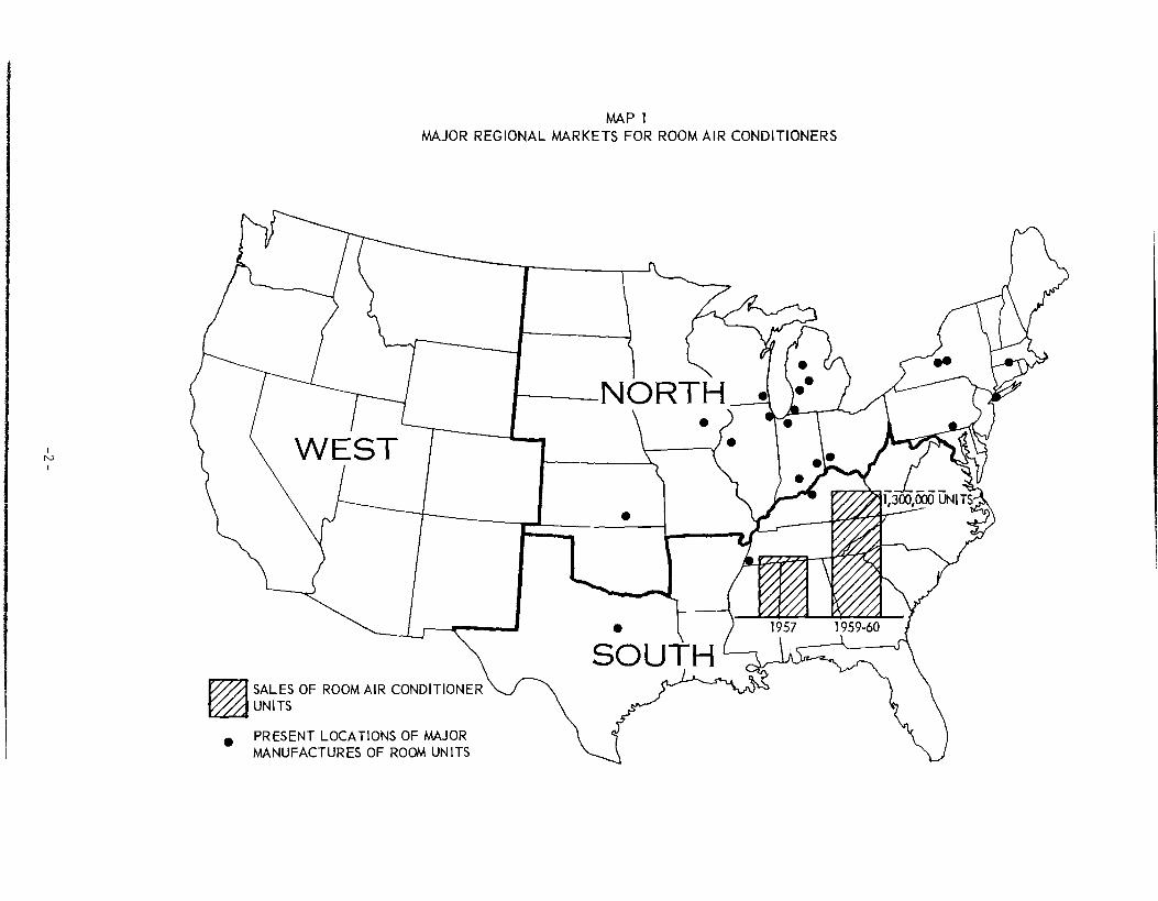
A SALES OF ROOM AIR CONDITIONER UNITS

PRESENT LOCATIONS OF MAJOR • MANUFACTURES OF ROOM UNITS

MAP 1 MAJOR REGIONAL MARKETS FOR ROOM AIR CONDITIONERS

I. INTRODUCTION

Many of the conclusions drawn in this report are based on the effects

of climatic and income differentials on the geographic distribution of room

air conditioner sales. That such effects do exist is nothing new; certainly

there is no intent here to belabor such an obvious point. Nevertheless,

further understanding of the market for this product can be gained by a re-

examination of these effects. Measurement of the extent of the interrela-

tionships among sales, income, and climate, in particular, can lead to more

definite and more fruitful conclusions than those intuitively accepted as

"obvious."

Mere intuition is often sufficient to describe and predict the behavior

of an individual; indeed, it is sometimes more appropriate than an analytical

tool that presupposes rational behavior. But in dealing with mass consumer

behavior with characteristics that differ among the various regions, a more

objective approach is needed. Such an approach is taken here, in that the

"obvious" is treated as an hypothesis.

The Second Section demonstrates that there is an empirical basis for

defining regional markets for room air conditioners. Statistical treatment

of sales data on a regional basis confirms the theoretical argument that

income and climate are among the major determinants of sales, and measures

the degree of influence exerted by these factors within the three regions de-

fined in Section II.

A forecast of 1959-60 production of room units is made in Section

with a very brief consideration of the southern region's probable share of

that market.

In Section IV, a simple scheme is constructed for the purpose of locating

the market center, based on the 1957 distribution of sales.

Section V devotes attention to the merits of the general vicinity of

Atlanta as regards plant location factors. More detailed information will be

provided as desired for any firm seeking a location meeting a particular set

of requirements.

II. THE MARKET ANALYSIS

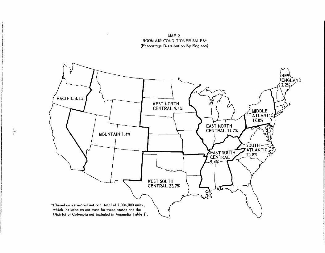
Sample sales data obtained from a large number of utilities, were used

to estimate sales of room air conditioners by states.-1/ Map 2, which follows,

shows the distribution of sales by Census regions. It is questionable, how-

ever, whether this definition of regions is appropriate for room air condi-

tioner markets. It is apparent that there is considerable variation among

the states in sales volume. A critical question, therefore is: What are

the factors which determine sales volume?

The answer could encompass many particulars, but it will be simplified

in the present case to consider only certain measurable factors. Certainly

the desire for comfort, in so far as a room air conditioner can provide it,

and the necessary purchasing power are two pertinent factors. Admittedly,

the conditions necessary for human comfort are complex, but relief from high

temperatures and excessive humidity are primary considerations.

Bosen and Thom of the U.S. Weather Bureau have made considerable progress

in developing measures of the need for summer cooling. Thom has recently pub-

lished values termed "cooling degree days" for a number of cities throughout

the United States. ?/ The cooling degree days variable is used in this study as

one of the factors influencing purchase decisions. Not all states could be

1/ Appendix I sets forth in detail the methodology used for these estimates.

2/ J. F. Bosen, Office of Climatology, U.S. Weather Bureau, Washington, D. C., has developed two linear equations which provide a Discomfort Index appropriate to the need for summer cooling. The first equation involves dry bulb and wet bulb temperatures; the second, dry bulb temperature and dew point temperature.

Earl C. Thom, Meteorologist, U.S. Weather Bureau, Washington, D. C., has proposed the Discomfort Index as a basis for measuring cooling degree days. A base figure of 60 is subtracted from the average Discomfort Index for each day, and the remaining values are accumulated into monthly and annual totals of cooling degree days.

The equations are:

(1) DI = 0.4(t d + tw) + 15

(2) DI = 0.55td + 0.2t

dp + 17.5

DI = Discomfort Index t

dp = Dew point temperature

t d = Dry bulb temperature

All t values are simultaneous

tw

= Wet bulb temperature

For further discussion, see "Cooling Degree Days," E. C. Thom, July 1958, p. 65ff., The Industrial Press, New York.

NEC., ENGLAND 2.2%,,ff

*(Based on estimated national total of 1,304,000 units, which includes an estimate for those states and the District of Columbia not included in Appendix Table 1).

MAP 2

ROOM AIR CONDITIONER SALES*

(Percentage Distribution By Regions)

considered in the analysis, since cooling degree data for some of them were

not available. Per capita income in the various states was used as a meas-

ure of purchasing power.

The analysis which follows is a study of the relationships between the

two factors--"climate" and income--and sales per thousand domestic customers

of the electric utilities. The method employed to measure these relation-

ships is multiple correlation, and the hypothesis is that sales are "dependent"

upon income and the climatic factor.

The basic data are given in Table I. The results of the analysis are

arranged in tabular form in Table II. Contrary to expectation, it will be

noted that in the aggregate, sales are negatively correlated with cooling de-

gree days. As will be seen, the aggregative analysis is somewhat deceiving,

in that the coefficients reflect implicitly the fact that most of the high

income states are in the North, and the states where air conditioning is most

needed or desirable are generally in the low-income group.1/

The aggregative analysis also suggests that a basis for developing more

appropriate regional definitions is needed for the purposes of this market

study. The basic concept in regional grouping is dual. First, the region must

be unbroken and continuous. Second, it must be relatively uniform in climate

or income. The question is whether regions can be defined in terms of geo-

graphic areas differing in income and climate characteristics.

The Regions

The various states were ranked according to per capita income and number

of cooling degree days, and then compared for similarities of state groupings.

There are patterns in these listings, although some slight modification is

necessary to preserve geographic grouping.

Two groups of states are well defined. The first consists of Arkansas,

Alabama, Florida, Georgia, Louisiana, Mississippi, North Carolina, South Caro-

lina, Tennessee and Texas. The second group is composed of Illinois, Massa-

chusetts, Michigan, Minnesota, Missouri, Nebraska, New York, North Dakota, Ohio

1/ When this is taken into account in the second order coefficients the negative correlation between sales and income

(r12.3) become somewhat smaller.

The final result (R1.23)'

which takes both factors into consideration simul-taneously, reflects a considerable degree of "improvement" over the lower order coefficients, i.e., it tends to better agreement with the hypothesis. These results are not particularly enlightening, except to serve as a contrast to the results obtained when the same methods are applied to the same data grouped as various regions.

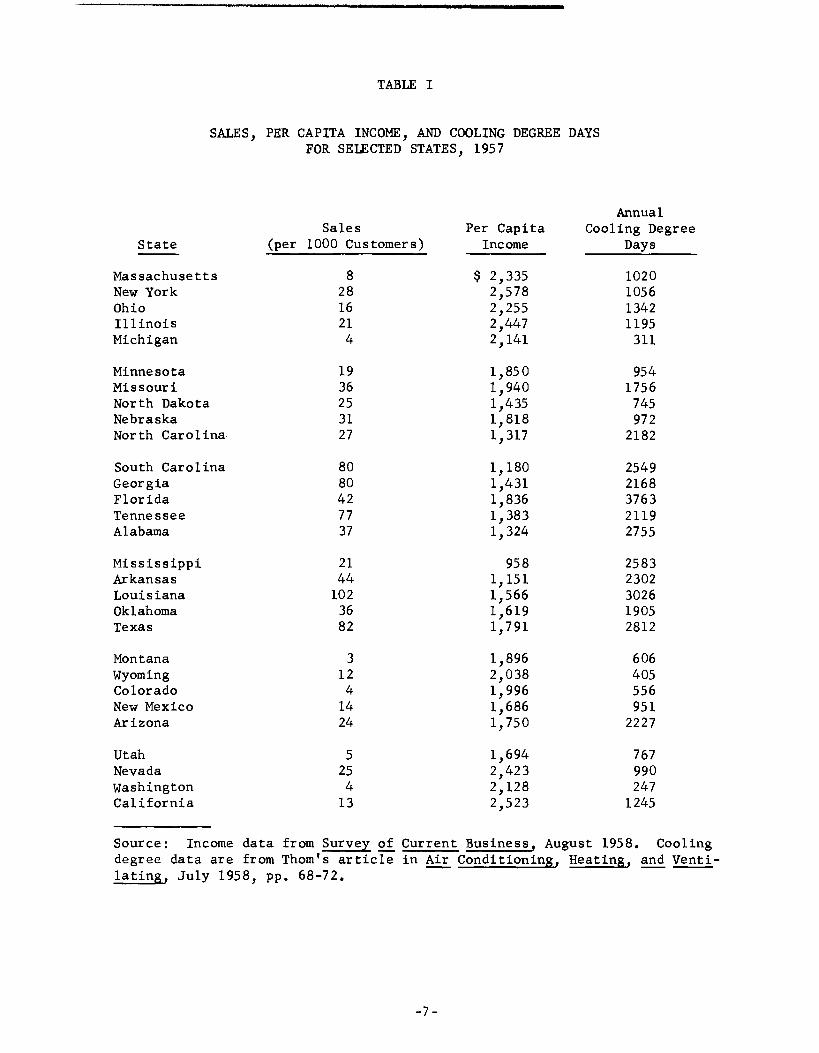
TABLE I

SALES, PER CAPITA INCOME, AND COOLING DEGREE DAYS FOR SELECTED STATES, 1957

Annual Sales Per Capita Cooling Degree

State (per 1000 Customers) Income Days

Massachusetts 8 $ 2,335 1020 New York 28 2,578 1056 Ohio 16 2,255 1342 Illinois 21 2,447 1195 Michigan 4 2,141 311

Minnesota 19 1,850 954 Missouri 36 1,940 1756 North Dakota 25 1,435 745 Nebraska 31 1,818 972 North Carolina 27 1,317 2182

South Carolina 80 1,180 2549 Georgia 80 1,431 2168 Florida 42 1,836 3763 Tennessee 77 1,383 2119 Alabama 37 1,324 2755

Mississippi 21 958 2583 Arkansas 44 1,151 2302 Louisiana 102 1,566 3026 Oklahoma 36 1,619 1905 Texas 82 1,791 2812

Montana 3 1,896 606 Wyoming 12 2,038 405 Colorado 4 1,996 556 New Mexico 14 1,686 951 Arizona 24 1,750 2227

Utah 5 1,694 767 Nevada 25 2,423 990 Washington 4 2,128 247 California 13 2,523 1245

Source: Income data from Survey of Current Business, August 1958. Cooling degree data are from Thom's article in Air Conditioning, Heating, and Venti-lating, July 1958, pp. 68-72.

and Oklahoma. A third group which is less well defined comprises Arizona,

California, Colorado, Montana, Nevada, New Mexico, Utah, Washington and

Wyoming.

A third ranking of states in order of total sales volume was used in

part as confirmation of these conclusions, and to aid in assigning states

for which no cooling degree data were available. Much the same pattern

emerges if states are checked off on a map of the United States as they

appear in this last ranking. See Map 3.

Thus, the two major regional markets seem to consist of one group of

states ranging eastward from the Great Plains through the Middle Atlantic

states up to New England, and a second group extending southward from the

Middle Atlantic states and over the Gulf Coast into Texas.

The Analysis

As a test of these regional definitions, correlation techniques may be

applied to the data for these regions, as was done for the national data. The

results appear in Table II. The differences from the overall or aggregative

analysis are of considerable importance.

First, the fact that differences do exist proves that the joint influ-

ence of climatic factors and income is of a different nature among the regions.

This establishes the case for regional market differentiation. The general

improvement of the correlation coefficients resulting from the market break-

down demonstrates the validity of the groupings, granted the a priori hypothe-

sis that income and the climatic factor are major determinants of sales.

Second, the nature of the differences has specific implications for

future market growth.

In the "South," income is clearly the dominant factor in determining

sales. The climatic factor does not specifically enter in, except in the

sense that the climate is uniformly such that a room air conditioner is de-

sirable.

In the other major market area, climate is dominant. Income is avail-

able, provided that climatic factors make an air conditioner sufficiently

desirable to warrant its purchase. Thus, occasional cool summers may depress

considerably the sales of room units in this region.

In the region composed of the Mountain and Pacific states, both factors

are considerations, but the climatic factor is more important.

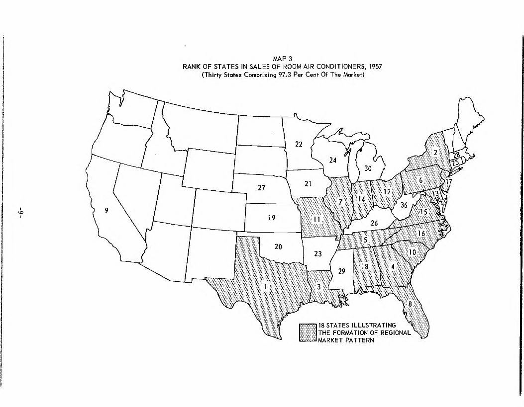
18 STATES ILLUSTRATING THE FORMATION OF REGIONAL MARKET PATTERN

MAP 3 RANK OF STATES IN SALES OF ROOM AIR CONDITIONERS, 1957

(Thirty States Comprising 97.3 Per Cent Of The Market)

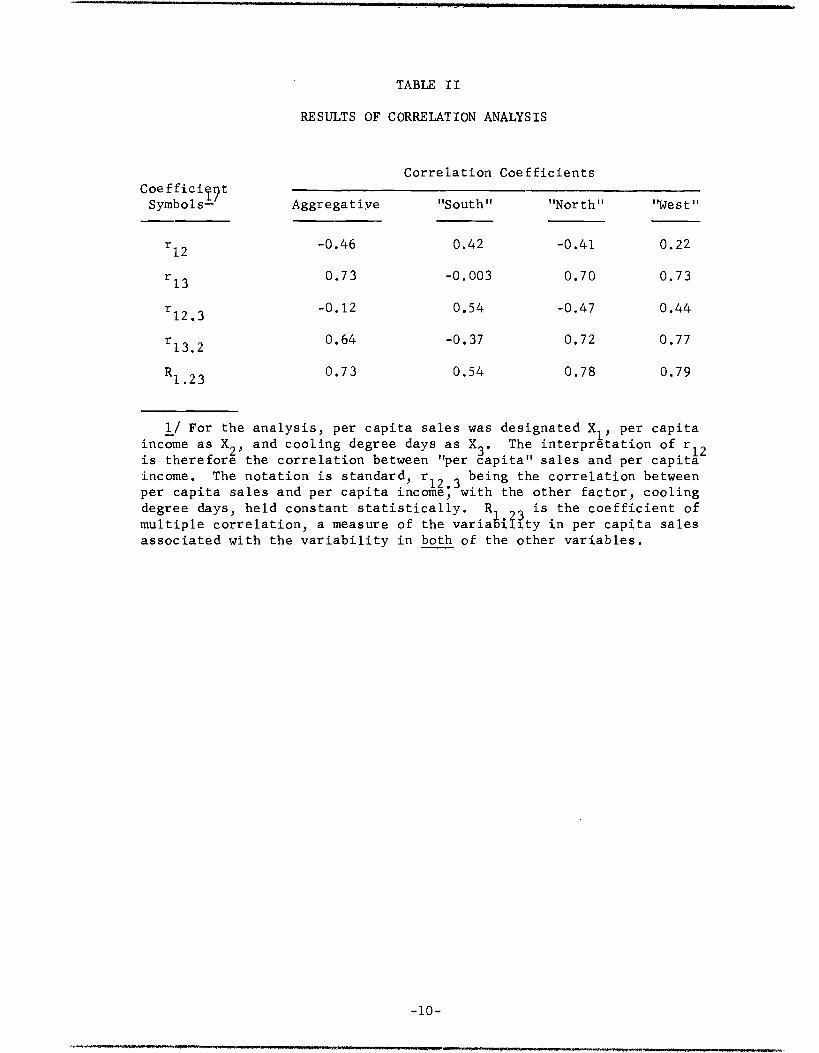
TABLE II

RESULTS OF CORRELATION ANALYSIS

Correlation Coefficients CoefficiT4t Symbols—f Aggregative "South" "North" "West"

r12

r13

r l2.3

r 13.2

R1.23

-0.46

0.73

-0.12

0.64

0.73

0.42

-0.003

0.54

-0.37

0.54

-0.41

0.70

-0.47

0.72

0.78

0.22

0.73

0.44

0.77

0.79

1/ For the analysis, per capita sales was designated X1, per capita

income as X2, and cooling degree days as X 3 . The interpretation of r 12 is therefore the correlation between "per capita" sales and per capita income. The notation is standard , r12.3 being the correlation between per capita sales and per capita income, with the other factor, cooling degree days, held constant statistically. R i 91 is the coefficient of multiple correlation, a measure of the variability in per capita sales associated with the variability in both of the other variables.

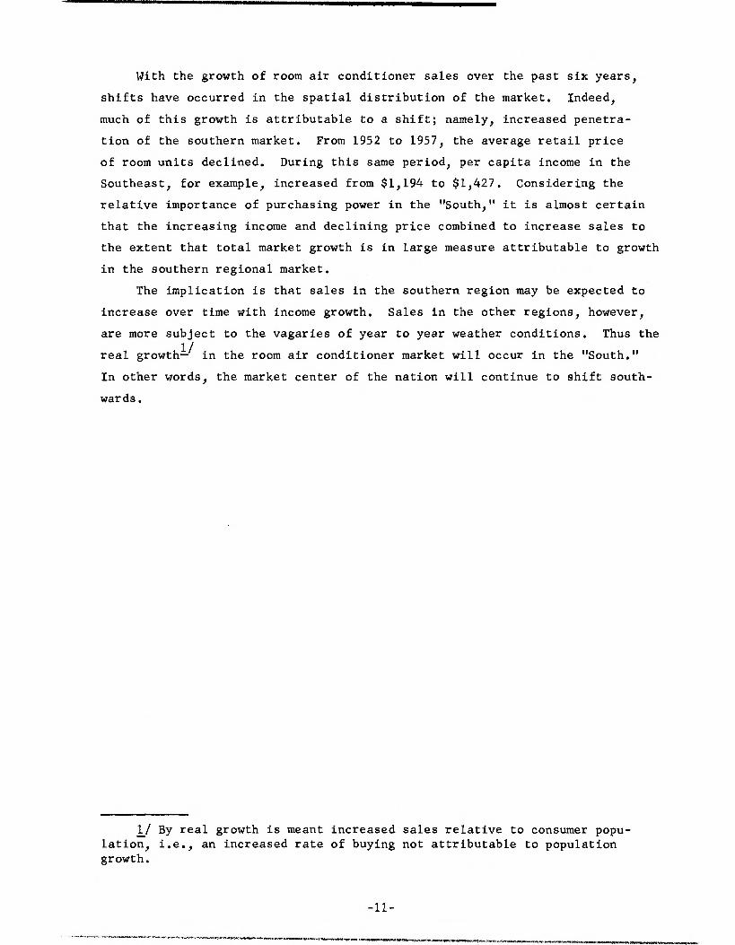
With the growth of room air conditioner sales over the past six years,

shifts have occurred in the spatial distribution of the market. Indeed,

much of this growth is attributable to a shift; namely, increased penetra-

tion of the southern market. From 1952 to 1957, the average retail price

of room units declined. During this same period, per capita income in the

Southeast, for example, increased from $1,194 to $1,427. Considering the

relative importance of purchasing power in the "South," it is almost certain

that the increasing income and declining price combined to increase sales to

the extent that total market growth is in large measure attributable to growth

in the southern regional market.

The implication is that sales in the southern region may be expected to

increase over time with income growth. Sales in the other regions, however,

are more subject to the vagaries of year to year weather conditions. Thus the

real growthli in the room air conditioner market will occur in the "South."

In other words, the market center of the nation will continue to shift south-

wards.

1/ By real growth is meant increased sales relative to consumer popu-lation, i.e., an increased rate of buying not attributable to population growth.

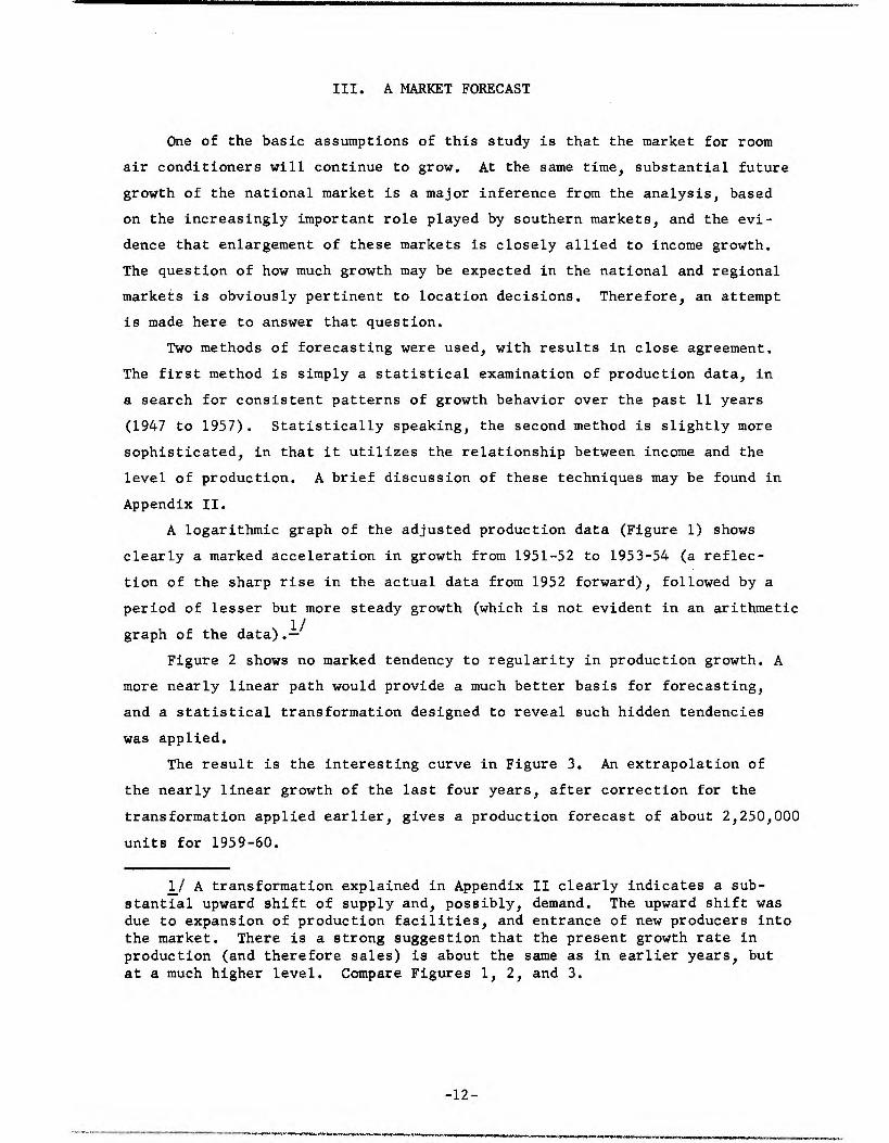
III. A MARKET FORECAST

One of the basic assumptions of this study is that the market for room

air conditioners will continue to grow. At the same time, substantial future

growth of the national market is a major inference from the analysis, based

on the increasingly important role played by southern markets, and the evi-

dence that enlargement of these markets is closely allied to income growth.

The question of how much growth may be expected in the national and regional

markets is obviously pertinent to location decisions. Therefore, an attempt

is made here to answer that question.

Two methods of forecasting were used, with results in close agreement.

The first method is simply a statistical examination of production data, in

a search for consistent patterns of growth behavior over the past 11 years

(1947 to 1957). Statistically speaking, the second method is slightly more

sophisticated, in that it utilizes the relationship between income and the

level of production. A brief discussion of these techniques may be found in

Appendix II.

A logarithmic graph of the adjusted production data (Figure 1) shows

clearly a marked acceleration in growth from 1951-52 to 1953-54 (a reflec-

tion of the sharp rise in the actual data from 1952 forward), followed by a

period of lesser but more steady growth (which is not evident in an arithmetic

graph of the data). 1/

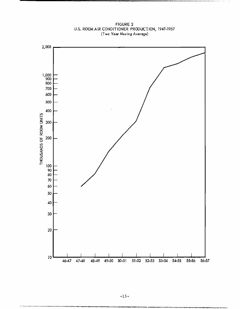
Figure 2 shows no marked tendency to regularity in production growth. A

more nearly linear path would provide a much better basis for forecasting,

and a statistical transformation designed to reveal such hidden tendencies

was applied.

The result is the interesting curve in Figure 3. An extrapolation of

the nearly linear growth of the last four years, after correction for the

transformation applied earlier, gives a production forecast of about 2,250,000

units for 1959-60.

1/ A transformation explained in Appendix II clearly indicates a sub-- stantial upward shift of supply and, possibly, demand. The upward shift was due to expansion of production facilities, and entrance of new producers into the market. There is a strong suggestion that the present growth rate in production (and therefore sales) is about the same as in earlier years, but at a much higher level. Compare Figures 1, 2, and 3.

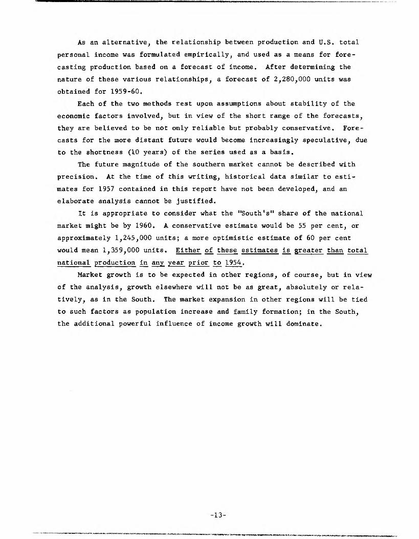
As an alternative, the relationship between production and U.S. total

personal income was formulated empirically, and used as a means for fore-

casting production based on a forecast of income. After determining the

nature of these various relationships, a forecast of 2,280,000 units was

obtained for 1959-60.

Each of the two methods rest upon assumptions about stability of the

economic factors involved, but in view of the short range of the forecasts,

they are believed to be not only reliable but probably conservative. Fore-

casts for the more distant future would become increasingly speculative, due

to the shortness (10 years) of the series used as a basis.

The future magnitude of the southern market cannot be described with

precision. At the time of this writing, historical data similar to esti-

mates for 1957 contained in this report have not been developed, and an

elaborate analysis cannot be justified.

It is appropriate to consider what the "South's" share of the national

market might be by 1960. A conservative estimate would be 55 per cent, or

approximately 1,245,000 units; a more optimistic estimate of 60 per cent

would mean 1,359,000 units. Either of these estimates is greater than total

national production in ELI year prior to 1954.

Market growth is to be expected in other regions, of course, but in view

of the analysis, growth elsewhere will not be as great, absolutely or rela-

tively, as in the South. The market expansion in other regions will be tied

to such factors as population increase and family formation; in the South,

the additional powerful influence of income growth will dominate.

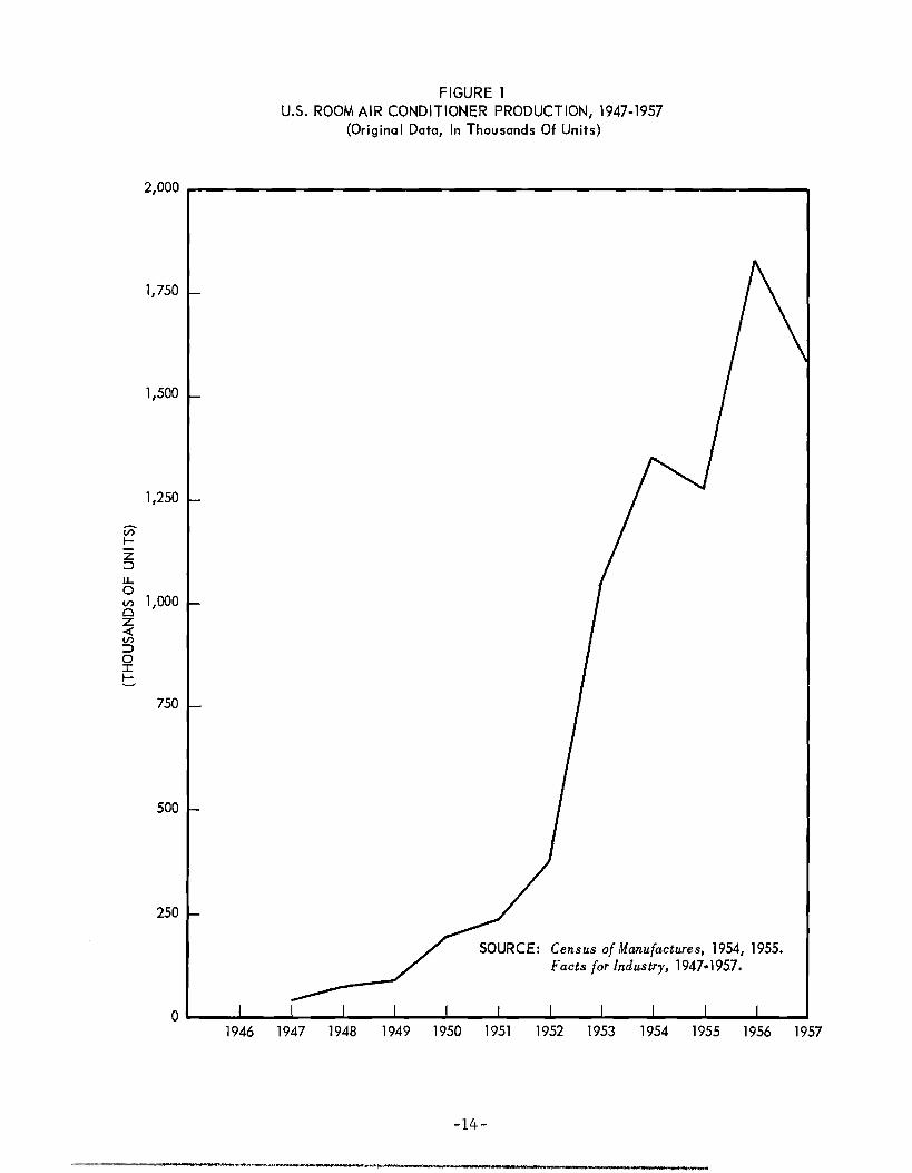
SOURCE: Census of Manufactures, 1954, 1955. Facts for Industry, 1947.1957.

1 I J 1 I I 1 I I I I

FIGURE 1 U.S. ROOM AIR CONDITIONER PRODUCTION, 1947-1957

(Original Data, In Thousands Of Units)

2,000

1,750

1,500

1,250

(7')

2 D U- 0

0 v.) 1,000 Z ,t( In D 0 2 I-

750

500

250

1946 1947 1948 1949 1950 1951 1952 1953 1954 1955 1956 1957

TH

OU

SAN

DS

OF

RO

OM

UN

ITS

2,000

1,000 900 800 700

600

500

400

300

200

100 90 80 70

50

40

30

60

20

10

FIGURE 2 U.S. ROOM AIR CONDITIONER PRODUCTION, 1947-1957

(Two Year Moving Average)

46.47 47-48 48-49 49-50 50.51 51-52 52-53 53-54 54-55 55-56 56.57

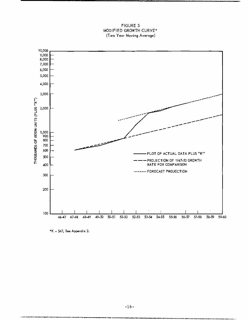
PLOT OF ACTUAL DATA PLUS "K"

---PROJECTION OF 1947-52 GROWTH — RATE FOR COMPARISON*

FORECAST PROJECTION

I I I I I I I I I I I I I

FIGURE 3 MODIFIED GROWTH CURVE*

(Two Year Moving Average)

10,000 9,000 8,000 7,000

6,000

5,000

4,000

3,000

'.' 2,000 _1 0_ 0 I— E m

O

•

1,000 ce 900

0 u_ 800 v) 700 0 < z 600 N 0 = 500 =

400

300

200

100 46-47 47-48 48-49 49-50 50.51 51-52 52-53 53-54 54-55 55-56 56-57 57-58 58-59 59-60

*K = 547, See Appendix 2.

IV. THE COMPARATIVE LOCATION STUDY

The cost of shipping an assembled room air conditioner includes freight

on sheet metal and hardware of the kind available almost everywhere. In addi-

tion, the unit's bulk includes empty space which, although necessary in air

flow design, is costly to transport. As a consequence, market orientation

of manufacturing plants affords an opportunity to reduce distribution costs

of the assembled unit.

Clearly, there must be an optimum plant location with respect to costs

of distribution. The total cost of distribution for a product manufactured

in a given location depends on the volume shipped to the various markets

served. Thus this cost is a function of the distance from the manufacturing

site to the various markets, weighted by the volume of units shipped to those

markets. If the volume shipped to each distribution point were known, a manu-

facturing site could be chosen in such a manner as to minimize the cost of dis-

tribution.

Appendix I sets forth estimates of sales by states. If these estimates

could be allocated to more specific locations, then comparisons could be made

between the location advantages of various manufacturing sites with respect

to market penetration (in terms of access).

Data of the kind and extent suitable for such comparisons are not avail-

able, but after certain simplifying assumptions, approximations may be

obtained. State sales data as such are not useful for comparative purposes,

as it would be difficult to select a single point within a state from which

distances to manufacturing sites would be representative statistically of the

whole state. An alternative is to select from each state major distribution

centers, allocate state sales proportionally to these centers, and compare their

distances from the various cities with plants. This is the method used here.

Selection of Distribution Centers

The problem becomes one of selecting the distribution centers and develop-

ing a suitable method of proportional allocation. In general, major distribu-

tion centers are also major population centers. From each state those metro-

politan areas were selected which account for at least 50 per cent of the

total metropolitan area population in that state. The 50 per cent level was

chosen simply to reduce the number of cities that would be involved, and con-

sequently reduce the amount of computation.

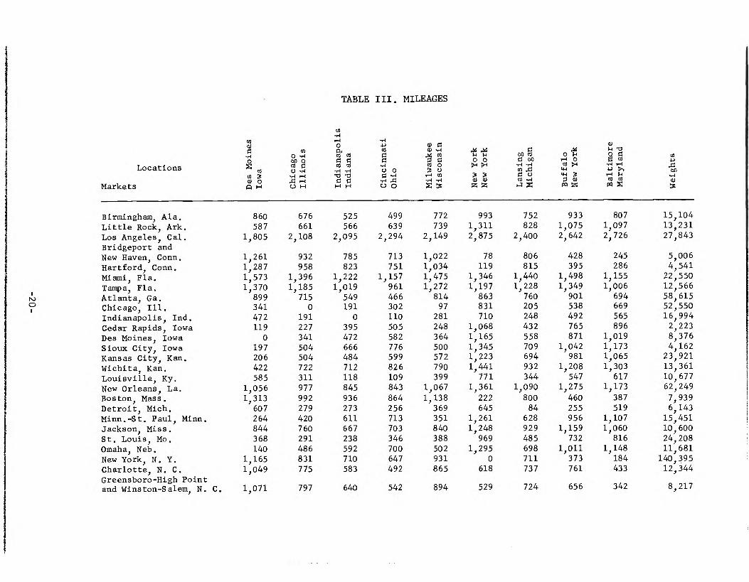
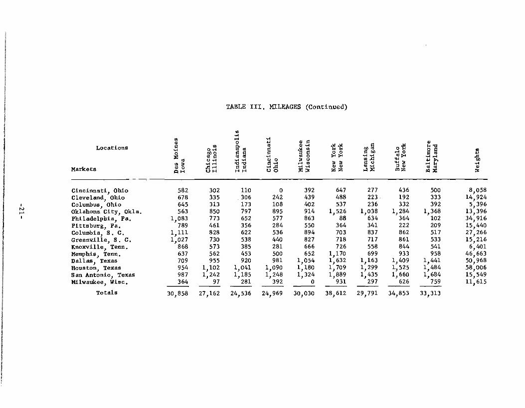
Forty-three cities-1/ were selected and, insofar as possible, distances

from these major distribution centers to cities with room air conditioner

plants were obtained. In some cases, present sites are in cities for which

distance tables would be very difficult to construct, and nearby major cities

were substituted. Highway mileages were used in this study primarily because

a considerable portion of room unit output is transported by truck. A mile-

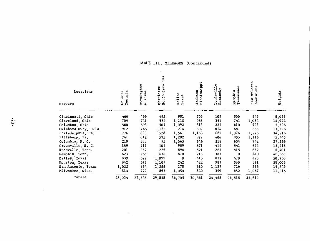
age table was constructed as shown in Table III. The column headings are

cities with plants or cities near plants of some of the major manufacturers

of room units, plus certain other cities used for comparative purposes. The

cities heading the rows are the selected distribution centers. The column

totals are the total mileage between plant sites, actual or hypothetical, and

the major markets in each state. If sales were the same in each of the

selected cities, the most favored site would obviously be the one with the

smallest column total (Louisville, Kentucky). Since sales are not uniformly

distributed, the matter is in doubt until the mileages in the body of the

table are weighted by the volume of shipments to each destination. The

"weights" are an approximation of sales in the various metropolitan areas.

They are derived by application of ratios to the estimates of state sales as

derived in Appendix I. The ratios are simply the percentages of the states'

total metropolitan area wholesale sales accounted for by the individual met-

ropolitan areas.

For example, the "weights" for the Miami and Tampa metropolitan areas

were derived as follows:

Estimated Unit Sales Sales of Merchant WholesWrs ("Weight") (Thousands of Dollars) —

Florida 52,600 $1,323,972

Miami (22,550) 567,534

Tampa-St. Pete (12,566) 316,265

Other metropolitan areas 440,173

Source: Census of Business, 1954, U.S. Department of Commerce

1/ The metropolitan areas of Baltimore, Maryland, Norfolk-Portsmouth and Richmond, Virginia, and the District of Columbia which should be included by the method of selection, were not used. Sufficient sample data for state sales estimates were not available.

For Miami, the estimate would be 567,534/1,323,972 x 52,600 or 22,550;

Tampa, 316,265/1,323,972 x 52,600 or 12,566. These two estimates are then

applied as "weights" to distances from Miami and Tampa to the cities heading

the columns.

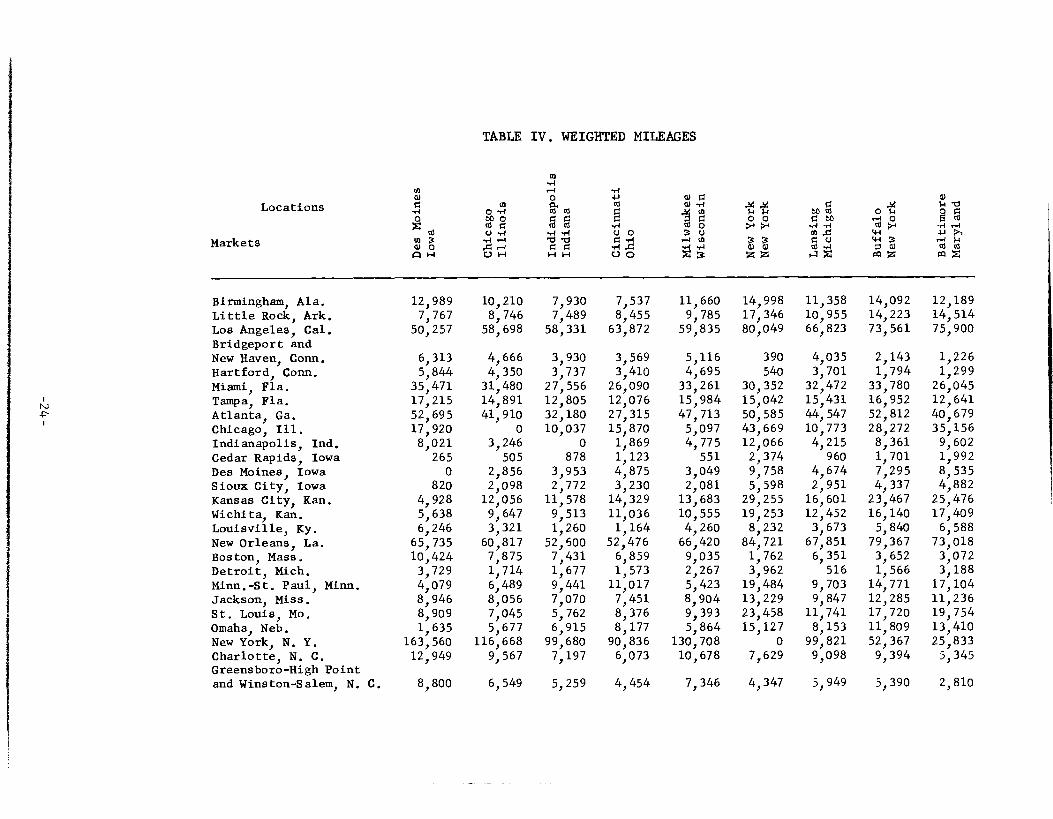
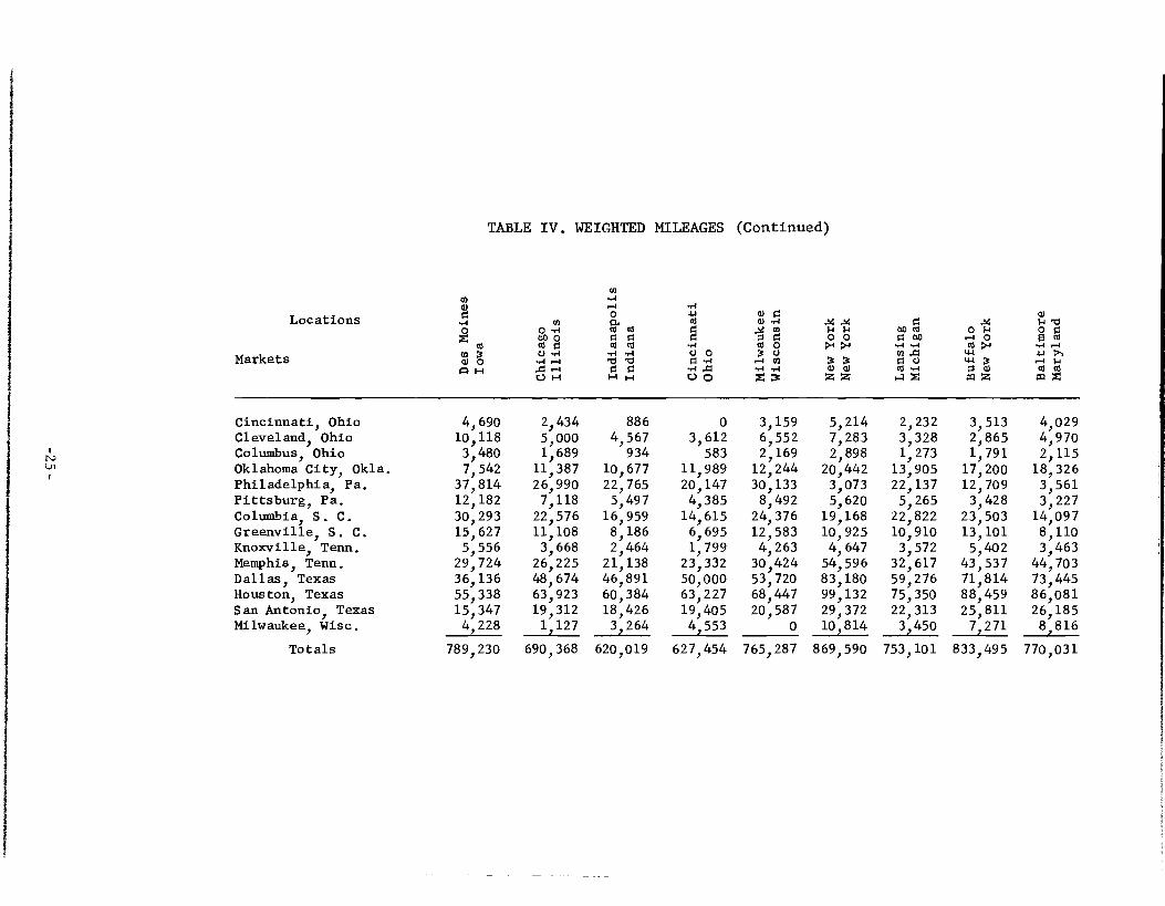
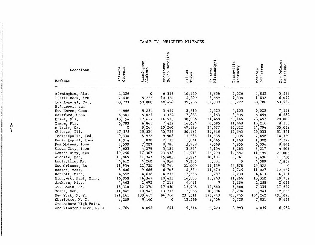
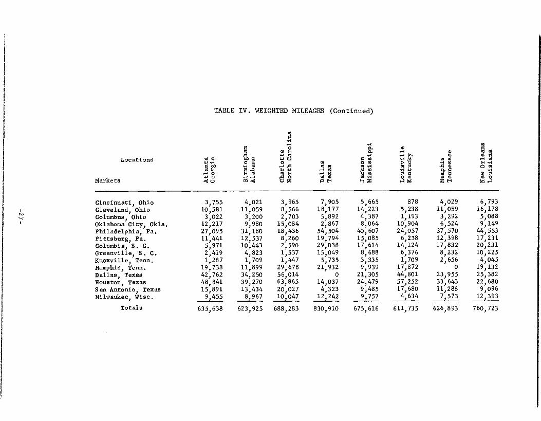
The entries in the distance table were multiplied by similarly derived

weights to obtain Table IV and summed as before. In this case, the distri-

bution of sales is such that the location most favored with respect to national

market penetration (given the 1957 national sales distribution as estimated

in Appendix I, Table I) is again Louisville, Kentucky. The rank of the first

six of the cities examined, in ascending order of weighted distances, is as

follows: Louisville, Kentucky; Indianapolis, Indiana; Birmingham, Alabama;

Memphis, Tennessee; Cincinnati, Ohio; and Atlanta, Georgia.

The reliability of the method of allocating sales among selected metro-

politan areas is supported to a considerable extent by the findings of the

LIFE Study of Consumer Expenditures in 1956. According to this survey,

metropolitan area residents accounted for 79 per cent of the total air condi-

tioner market; non-metropolitan area residents accounted for 21 per cent.

The South was the only exception to this national pattern. In that region,

sales were about equally divided between the two groups. This indicates that

coverage of the southern markets involves a greater number of distribution

points than in other regions, and that some advantage could be obtained by

locating near these points. A further inference is that the results obtained

in the location analysis possibly do not place the national market center as

far south as it actually is. If more southern distribution centers had been

included in the computations, the relative positions of the hypothetical

southern plant locations would tend to improve, since the majority of the addi-

tional markets lie south of those chosen for the computations, and therefore

farther from the present actual plant sites.

The implication of a southward shifting market center for future manufac-

turing plant location decisions is clear. If competitive advantages can be

obtained by locating near the market center, then relocation or branch plant

expansion of existing production facilities now elsewhere will result in a

larger share of a growing market.

For practical purposes, the knowledge that the market center is shifting

southward is sufficient to enable most manufacturers to improve significantly

1/ LIFE Study of Consumer Expenditures, TIME, Incorporated, 1957.

Cincinnati

Des Moin

es

Markets

Locations

r-4 0

cd

0 rl W 0 OD 0 0 0 0 0 0 0 U.A

0 C H 0 C. H 0 H H H

o ri

o,.0

cu o w .,-1

0 0 0

u H M rirl Z

.1c .x 0 0

>4 >4

3 3 01 0) Z Z

0 0 b

.1-1 rl p

5 X 0 U 0 rl

1-3 Z

x 1-1 0 0 >-I

44 W 0 (3) M Z

al $.4 -cs 0 0 6 0

• H L./ H P 0 0 M Z

X ao U

TABLE III. MILEAGES

Birmingham, Ala. Little Rock, Ark. Los Angeles, Cal. Bridgeport and New Haven, Conn.Hartford, Conn. Miami, Fla. Tampa, Fla. Atlanta, Ga. Chicago, Ill. Indianapolis, Ind. Cedar Rapids, Iowa Des Moines, Iowa Sioux City, Iowa Kansas City, Kan. Wichita, Kan. Louisville, Ky. New Orleans, La. Boston, Mass. Detroit, Mich. Minn.-St. Paul, Minn. Jackson, Miss. St. Louis, Mo. Omaha, Neb. New York, N. Y. Charlotte, N. C. Greensboro-High Point and Winston-Salem, N. C.

860 587

1,805

1,261 1,287 1,573 1,370

899 341 472 119

0 197 206 422 585

1,056 1,313

607 264 844 368 140

1,165 1,049

1,071

676 661

2,108

932 958

1,396 1,185

715 0

191 227 341 504 504 722 311 977 992 279 420 760 291 486 831 775

797

525 566

2,095

785 823

1,222 1,019

549 191

0 395 472 666 484 712 118 845 936 273 611 667 238 592 710 583

640

499 639

2,294

713 751

1,157 961 466 302 110 505 582 776 599 826 109 843 864 256 713 703 346 700 647 492

542

772 739

2,149

1,022 1,034 1,475 1 ,272

814 97

281 248 364 500 572 790 399

1,067 1,138

369 351 840 388 502 931 865

894

993 1,311 2,875

78 119

1,346 1, 197

863 831 710

1,068 1,165 1,345 1,223 1,441

771 1,361

222 645

1,261 1,248

969 1,295

0 618

529

752 828

2,400

806 815

1,440 1 ,228

760 205 248 432 558 709 694 932 344

1,090 800 84

628 929 485 698 711 737

724

933 1,075 2,642

428 395

1,498 1, 349

901 538 492 765 871

1,042 981

1,208 547

1,275 460 255 956

1,159 732

1,011 373 761

656

807 1,097 2,726

245 286

1,155 1,006

694 669 565 896

1,019 1,173 1,065 1,303

617 1,173

387 519

1,107 1,060

816 1,148

184 433

342

15,104 13,231 27,843

2 2 ,550

1552 :,55566 g 16,994 2,223 8,376 4,162

23,921 13,361 10,677 62,249 7,939 6,143

15,451 10,600 24,208 11,681

140,395 12,344

8,217

a) 0 xi r0 b0 0 0 14 0 tm -I o B ,a ,a 4 1 _5 A g 1) bo

WI 1-1 14 .1-1 0 a) ai 0 1,11 Z P=1 Z 3

277 436 500 8,058 223 192 333 14,924 236 332 392 5,396

1,038 1,284 1,368 13,396 634 364 102 34,916 341 222 209 15,440 837 862 517 27,266 717 861 533 15,216 558 844 541 6,401 699 933 958 46,663

1,163 1,409 1,441 50,968 1,299 1,525 1,484 58,006 1,435 1,660 1,684 15,549

297 626 759 11,615

29,791 34,853 33,313

1 N.) 1-, o

Locations

Markets

co w PI ,-1

o W

m 3 a) c) A H

o -,4 bo o 0 0 0 .,-1

N-I 1-1 A ,-1 C.) H

-raj

TABLE III. MILEAGES (Continued)

ca 44 .-1 44 o 4.1 w 0

0 a) dal

..W Ed Ed 0 ..sd al 14 14 o o 0 0 0 o o 0 0 ,1 0 0 7+ ..-1.,-1 u o 3 w •0 'V 0 44 1-1 M o 0 ..-1 A a) a) H H 0 0 .1 1 ZZ

Cincinnati, Ohio Cleveland, Ohio Columbus, Ohio Oklahoma City, Okla. Philadelphia, Pa. Pittsburg, Pa. Columbia, S. C. Greenville, S. C. Knoxville, Tenn. Memphis, Tenn. Dallas, Texas Houston, Texas San Antonio, Texas Milwaukee, Wisc.

Totals

582 678 645 563

1,083 789

1,111 1,027

868 637 709 954 987 364

302 335 313 850 773 461 828 730 573 562 955

1,102 1,242

97

110 306 173 797 652 356 622 538 385 453 920

1,041 1,185

281

0 242 108 895 577 284 536 440 281 500 981

1,090 1,248

392

392 439 402 914 863 550 894 827 666 652

1,054 1,180 1,324

0

647 488 537

1,526 88

364 703 718 726

1,170 1,632 1,709 1,889

931

30,858 27,162 24,536 24,969 30,030 38,612

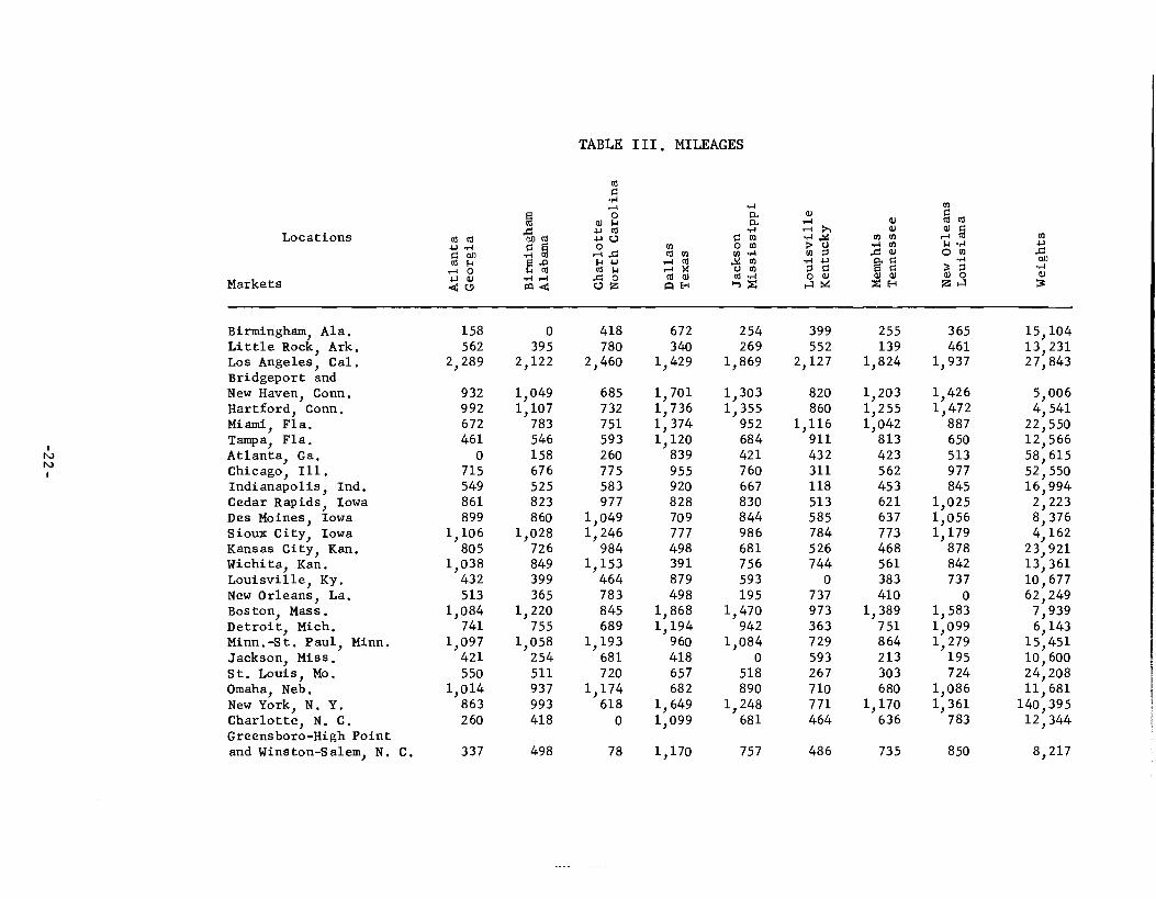
TABLE III . MILEAGES

Markets

Locations

Char

lotte

North C

aroli

na

fa. ta. 1-1 W

.r4 1-1 W

0 M •1-1 ,M W M

d W Cd .1-1 0 W W W

A H in Z 1-1 Z H New Or

lean

s Lo

uis

iana

U

co

a)

158 0 418 672 254 399 255 365 15,104 562 395 780 340 269 552 139 461 13,231

2,289 2,122 2,460 1,429 1,869 2,127 1,824 1,937 27,843

932 1,049 685 1,701 1,303 820 1,203 1,426 5,006 992 1,107 732 1,736 1,355 860 1,255 1,472 4,541 672 783 751 1,374 952 1,116 1,042 887 22,550 461 546 593 1,120 684 911 813 650 12,566

0 158 260 839 421 432 423 513 58,615 715 676 775 955 760 311 562 977 52,550 549 525 583 920 667 118 453 845 16,994 861 823 977 828 830 513 621 1,025 2,223 899 860 1,049 709 844 585 637 1,056 8,376

1,106 1,028 1,246 777 986 784 773 1,179 4,162 805 726 984 498 681 526 468 878 23,921

1,038 849 1,153 391 756 744 561 842 13,361 432 399 464 879 593 0 383 737 10,677 513 365 783 498 195 737 410 0 62,249

1,084 1,220 845 1,868 1,470 973 1,389 1,583 7,939 741 755 689 1,194 942 363 751 1,099 6,143

1,097 1,058 1,193 960 1,084 729 864 1,279 15,451 421 254 681 418 0 593 213 195 10,600 550 511 720 657 518 267 303 724 24,208

1,014 937 1,174 682 890 710 680 1,086 11,681 863 993 618 1,649 1,248 771 1,170 1,361 140,395 260 418 0 1,099 681 464 636 783 12,344

337 498 78 1,170 757 486 735 850 8,217

Birmingham, Ala. Little Rock, Ark. Los Angeles, Cal. Bridgeport and New Haven, Conn. Hartford, Conn. Miami, Fla. Tampa, Fla. Atlanta, Ga. Chicago, Ill. Indianapolis, Ind. Cedar Rapids, Iowa Des Moines, Iowa Sioux City, Iowa Kansas City, Kan. Wichita, Kan. Louisville, Ky. New Orleans, La. Boston, Mass. Detroit, Mich. Minn.-St. Paul, Minn. Jackson, Miss. St. Louis, Mo. Omaha, Neb. New York, N. Y. Charlotte, N. C. Greensboro-High Point and Winston-Salem, N. C.

o i

W .-9 m m ..-1 m k •,-1 4.)

.0 0 0 al 4

.4-1 W

P,' E 0 "

0 0 0 Z. i Z1-3

843 8,058 1,084 14,924

943 5,396 683 13,396

1,276 34,916 1,116 15,440

742 27,266 672 15,216 632 6,401 410 46,663 498 50,968 391 58,006 585 15,549

1,067 11,615

35,612

500 741 610 487

1,076 803 654 541 415

0 470 580 726 652

26,818

1 Iv u.)

Locations

Markets

0 0 4.1 ..4 0 Pa 0 14

•.-I 0 410) ..:4 0

TABLE III. MILEAGES

as 0

..-1 ....I

M o W W .0 4.1 0 al 0 4-1 r_.1 co

r-I .0 0 0

•N 1 14 4.1 ,.-1 W m 14 ,4 14

...I .-1 4 0 W W Pfd' 0Z MI E-I

(Continued)

..-I m O.

w .,-1 ■-4 P.,

0 m n4 ,..V O a) > c) 03,-1 0 0

..s4 0 ..-1 4.1 0 m 0 . CO ..-1 0 I0 In Z 1-4 c4

Cincinnati, Ohio Cleveland, Ohio Columbus, Ohio Oklahoma City, Okla. Philadelphia, Pa. Pittsburg, Pa. Columbia, S. C. Greenville, S. C. Knoxville, Tenn. Memphis, Tenn. Dallas, Texas Houston, Texas San Antonio, Texas Milwaukee, Wisc.

Totals

466 709 560 912 776 741 219 159 201 423 839 842

1,022 814

499 741 593 745 893 812 383 317 267 255 672 677 864 772

492 574 501

1,126 528 535 95

101 226 636

1,099 1,101 1,288 865

981 1,218 1,092

214 1,561 1,282 1,065

989 896 470

0 242 278

1,054

703 953 813 602

1,163 977 646 571 521 213 418 422 610 840

109 351 221 814 689 404 518 419 267 383 879 987

1,137 399

28,034 27,545 29,858 36,705 30,461 24,468

W

0 N

m 0.'4 W 0 af 0 0 d NH ...0 H OH

m .,-1 H o a W W

g g rl.r1 'Li Ti 0 0 HH

ri 4-1 o 0 0

-,4 0 0 0,-I ri .0 0 0

m o W -,4 .M M 0 0 Et o

0 H M 4-1 H Z'3

-- -- H H 0 0

>4 3 3 W W Z Z

0 W W 0 W

-,4 .,-1 CO ,0 0 0 W .1-1 4Z

x0 H r-I 0 as >4

W W 0 M M Z

m H yr) 0 0 5 Et

-,4 rA .I.J H $4 W W

CA Z Markets

Locations

Des Moines

TABLE IV. WEIGHTED MILEAGES

10,210 7,930 7,537 11,660 14,998 11,358 14,092 12,189 8,746 7,489 8,455 9,785 17,346 10,955 14,223 14,514

58,698 58,331 63,872 59,835 80,049 66,823 73,561 75,900

4,666 3,930 3,569 5,116 390 4,035 2,143 1,226 4,350 3,737 3,410 4,695 540 3,701 1,794 1,299

31,480 27,556 26,090 33,261 30,352 32,472 33,780 26,045 14,891 12,805 12,076 15,984 15,042 15,431 16,952 12,641 41,910 32,180 27,315 47,713 50,585 44,547 52,812 40,679

0 10,037 15,870 5,097 43,669 10,773 28,272 35,156 3,246 0 1,869 4,775 12,066 4,215 8,361 9,602

505 878 1,123 551 2,374 960 1,701 1,992 2,856 3,953 4,875 3,049 9,758 4,674 7,295 8,535 2,098 2,772 3,230 2,081 5,598 2,951 4,337 4,882

12,056 11,578 14,329 13,683 29,255 16,601 23,467 25,476 9,647 9,513 11,036 10,555 19,253 12,452 16,140 17,409 3,321 1,260 1,164 4,260 8,232 3,673 5,840 6,588

60,817 52,500 52,476 66,420 84,721 67,851 79,367 73,018 7,875 7,431 6,859 9,035 1,762 6,351 3,652 3,072 1,714 1,677 1,573 2,267 3,962 516 1,566 3,188 6,489 9,441 11,017 5,423 19,484 9,703 14,771 17,104 8,056 7,070 7,451 8,904 13,229 9,847 12,285 11,236 7,045 5,762 8 , 376 9 , 393 23,458 11,741 17,720 19,754 5,677 6,915 8,177 5,864 15,127 8,153 11,809 13,410

116,668 99,680 90,836 130,708 0 99,821 52,367 25,833 9,567 7,197 6,073 10,678 7,629 9,098 9,394 5,345

6,549 5,259 4,454 7,346 4,347 5,949 5,390 2,810

Birmingham, Ala. 12,989 Little Rock, Ark. 7,767 Los Angeles, Cal. 50,257 Bridgeport and New Haven, Conn. 6,313 Hartford, Conn. 5,844 Miami, Fla. 35,471 Tampa, Fla. 17,215 Atlanta, Ga. 52,695 Chicago, Ill. 17,920 Indianapolis, Ind. 8,021 Cedar Rapids, Iowa 265 Des Moines, Iowa 0 Sioux City, Iowa 820 Kansas City, Kan. 4,928 Wichita, Kan. 5,638 Louisville, Ky. 6,246 New Orleans, La. 65,735 Boston, Mass. 10,424 Detroit, Mich. 3,729 Minn.-St. Paul, Minn. 4,079 Jackson, Miss. 8,946 St. Louis, Mo. 8,909 Omaha, Neb. 1,635 New York, N. Y. 163,560 Charlotte, N. C. 12,949 Greensboro-High Point and Winston-Salem, N. C. 8,800

U) 0

"-i 4-7 0

0 0 0 60 0 0 0 0 0 0 0 W ,-;

.,-4 U 0 0 "0 H 0 ..-1 A

O H H H 0 0

Markets

Locations

Des Moin

es

0 a) 7-7 '0

60 0

0 74 0

0 0 m >1

ci7 4-1 0 7-1

M 0 W 1-1 M M

of

1 4

.4 Wisconsin

7-1 7-1 0 0 >4 >4 3 3 W 0 z z

TABLE IV. WEIGHTED MILEAGES (Continued)

U)

Cincinnati, Ohio Cleveland, Ohio Columbus, Ohio Oklahoma City, Okla. Philadelphia, Pa. Pittsburg, Pa. Columbia, S. C. Greenville, S. C. Knoxville, Tenn. Memphis, Tenn. Dallas, Texas Houston, Texas San Antonio, Texas Milwaukee, Wisc.

Totals

4,690 2,434 886 0 3,159 5,214 2,232 3,513 4,029 10,118 5,000 4,567 3,612 6,552 7,283 3,328 2,865 4,970 3,480 1,689 934 583 2,169 2,898 1,273 1,791 2,115 7,542 11,387 10,677 11,989 12,244 20,442 13,905 17,200 18,326

37,814 26,990 22,765 20,147 30,133 3,073 22,137 12,709 3,561 12,182 7,118 5,497 4,385 8,492 5,620 5,265 3,428 3,227 30,293 22,576 16,959 14,615 24,376 19,168 22,822 23,503 14,097 15,627 11,108 8,186 6,695 12,583 10,925 10,910 13,101 8,110 5,556 3,668 2,464 1,799 4,263 4,647 3,572 5,402 3,463

29,724 26,225 21,138 23,332 30,424 54,596 32,617 43,537 44,703 36,136 48,674 46,891 50,000 53,720 83,180 59,276 71,814 73,445 55,338 63,923 60,384 63,227 68,447 99,132 75,350 88,459 86,081 15,347 19,312 18,426 19,405 20,587 29,372 22,313 25,811 26,185 4,228 1

L___ 127 3

I____ 264 4I__ 553 0 10

---L--- 814 3

L___ 450 --- 7 , 271 8,816

789,230 690,368 620,019 627,454 765,287 753,101 833,495 770,031 869,590

Locations

Markets

0 0 1-, .1-I 0 (30 0 14

0 CU

.4 0

TABLE IV. WEIGHTED MILEAGES

w cod

W 0 4.1 M

g 0

cd DI

'Pc) 04..) 1-1 0 P .-I M

co .4 A P

a a

.,4 0 M 0 W co .1-1

..- 0 C.) IA

I-, Z

W ,-I .-t ›, -.-I ,.. > 0 CO 0

.m1 .1..) 0 0

14

W W

M W .1-1 co X W e•

0

Z El

0 0 0

.-IW 0

0 i.4 .14 0 0

rf

W ■-10

Birmingham, Ala. 2,386 0 6,313 10,150 3,836 6,026 3,852 5,513 Little Rock, Ark. 7,436 5,226 10,320 4,499 3,559 7,304 1,832 6,099 Los Angeles, Cal. 63,733 59,080 68,494 39,786 52,039 59,222 50,786 53,932 Bridgeport and New Haven, Conn. 4,666 5,251 3,429 8,515 6,523 4,105 6,022 7,139 Hartford, Conn. 4,505 5,027 3,324 7,883 6,153 3,905 5,699 6,684 Miami, Fla. 15,154 17,657 16,935 30,984 21,468 25,166 23,497 20,002

1 NJ o-N

Tampa, Fla. Atlanta, Ga.

5,793 0

6,861 9,261

7,452 15,240

14,074 49,178

8,595 24,677

11,448 25,322

10,216 24,794

8,168 30,069

Chicago, Ill. 37,573 35,524 40,726 50,185 39,938 16,343 29,533 51,341 Indianapolis, Ind. 9,330 8,922 9,908 15,634 11,335 2,005 7,698 14,360 Cedar Rapids, Iowa 1,914 1,830 2,172 1,841 1,845 1,140 1,380 2,279 Des Moines, Iowa 7,530 7,203 8,786 5,939 7,069 4,900 5,336 8,845 Sioux City, Iowa 4,603 4,279 5,186 3,234 4,104 3,263 3,217 4,907 Kansas City, Kan. 19,256 17,367 23,538 11,913 16,290 12,582 11,195 21,003 Wichita, Kan. 13,869 11,343 15,405 5,224 10,101 9,941 7,496 11,250 Louisville, Ky. 4,612 4,260 4,954 9,385 6,331 0 4,089 7,869 New Orleans, La. 31,934 22,720 48,741 31,000 12,139 45,878 25,522 0 Boston, Mass. 8,606 9,686 6,708 14,830 11,670 7,725 11,027 12,567 Detroit, Mich. 4,552 4,638 4,233 7,335 5,787 2,230 4,613 6,751 Minn.-St. Paul, Minn. 16,950 16,347 18,433 14,833 16,749 11,264 13,350 19,762 Jackson, Miss. 4,463 2,692 7,219 4,431 0 6,286 2,258 2,067 St. Louis, Mo. 13,314 12,370 17,430 15,905 12,540 6,464 7,335 17,527 Omaha, Neb. 11,845 10,945 13,713 7,966 10,396 8,294 7,943 12,686 New York, N. Y. 121,161 139,412 86,764 231,511 175,213 108,245 164,262 191,078 Charlotte, N. C. 3,209 5,160 0 13,566 8,406 5,728 7,851 9,665 Greensboro-High Point and Winston-Salem, N. C. 2,769 4,092 641 9,614 6,220 3,993 6,039 6,984

1 r...) --,1

Locations

Markets

TABLE IV. WEIGHTED MILEAGES (Continued)

0 -1 "4 o

0 14 o. a.

'boo 4i ...4

w w 0 4.) C.) 0 M 4-1 "4 q 0 al 0 0 0 01) g .-1 .0 of m m...1 ca :4 EI 14 4-1 ,4 W .. 0 ,4 0 0 IA .--I )4 U M 4..) 4)

71:14 :44 A 0 ca aJ 0 -.4

-00 U7 A P I-, Z

a, .-1 ,-1 P, "4 ,.. > 0 0 0

"4 u 0 0 0 W

1-1 W

a) m M

...4 m A W

ff. 0 W W Z P

w i ca

o .-1 0 ►4 "4 0 to

"4 3 0 W 0 Z e-1

Cincinnati, Ohio Cleveland, Ohio Columbus, Ohio Oklahoma City, Okla. Philadelphia, Pa. Pittsburg, Pa. Columbia, S. C. Greenville, S. C. Knoxville, Tenn. Memphis, Tenn. Dallas, Texas Houston, Texas San Antonio, Texas Milwaukee, Wisc.

Totals

3,755 10,581 3,022 12,217 27,095 11,441 5,971 2,419 1,287

19,738 42,762 48,841 15,891 9I- 455

4,021 11,059 3,200 9,980

31,180 12,537 10,443 4,823 1,709

11,899 34,250 39,270 13,434

8I___ 967

3,965 8,566 2,703

15,084 18,436 8,260 2,590 1,537 1,447

29,678 56 , 014 63,865 20,027 10L- 047

7,905 18,177 5,892 2,867

54,504 19,794 29,038 15,049 5,735

21,932 0

14,037 4,323

12L- 242

5,665 14,223 4,387 8,064

40,607 15,085 17,614 8,688 3,335 9,939

21,305 24,479 9,485 9L___ 757

878 5,238 1,193

10,904 24,057 6,238

14,124 6,376 1,709

17,872 44,801 57,252 17,680 4L- 634

4,029 11,059 3,292 6,524

37,570 12,398 17,832 8,232 2,656

0 23,955 33,643 11,288 7L--- 573

6,793 16,178 5,088 9,149

44,553 17,231 20,231 10,225 4,045 19,132 25,382 22,680 9,096

12L-- 393

635,638 623,925 688,283 830,910 675,616 611,735 626,893 760,723

their competitive positions in either the national or the southern regional

market. In the process they would gain any advantages to be offered by

newer production equipment and layout resulting from relocation or expansion

of production facilities.

The structure of freight rates, which often involves zones of equal cost,

makes it unnecessary to locate in a mathematically determined position to

obtain the desired transportation advantages. From the more practical point

of view, it is sufficient to choose a location near the market center which

has other desirable location advantages, such as good transportation facili-

ties and a plentiful labor supply with the necessary skills or trainability.

A manufacturer who wishes to concentrate primarily on regional sales,

should choose a southern location for much the same reasons. A well chosen

southern location would obtain regional market advantages, and would be near

the area toward which the national market center is moving. Such a location

would enable a producer to improve national penetration over time.

Regional specialization is not feasible unless the regional market in

question is sufficient to absorb a major part of the manufacturer's output,

and has enough growth potential to support planned increases in output. Of

the two regions which meet the first requisite, the South is undoubtedly in a

more favored position, as it has the greater growth potential. If regional

specialization is at all desirable, there is little doubt of the choice between

regions.

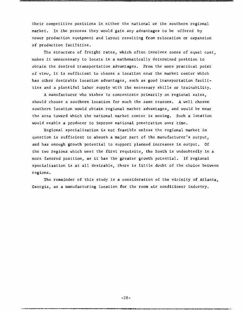
The remainder of this study is a consideration of the vicinity of Atlanta,

Georgia, as a manufacturing location for the room air conditioner industry.

V. ATLANTA AS A LOCATION FOR THE ROOM AIR CONDITIONER INDUSTRY

Of the first six cities in rank of nearness to the national market

center,-1/ only three lie south of Louisville: Birmingham, Memphis, and

Atlanta. These are the cities which will improve their positions as the

market center shifts southward. Of these three, Atlanta has the advantage

of being approximately equidistant from the East Texas-Gulf Coast markets

and the Middle Atlantic-Eastern Seaboard markets, a fact of some importance

in terms of transport time. Also, Atlanta has better developed transport-

distribution facilities. Of course, a realistic plant location decision

would have to be based on additional factors, such as desirable site avail-

ability and a study of the actual dollar costs of distribution for each of

the three cities. As a preliminary step in that direction, certain general

factors will be given attention in this report.

The Labor Market

Among the many factors to be considered in a location decision, the

supply of suitable labor is perhaps one of the most important. The Atlanta

labor supply is favorable for industry.

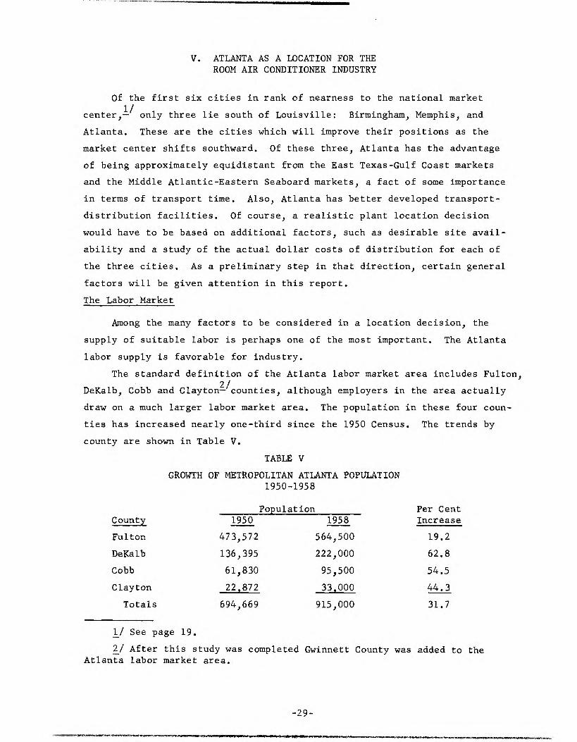
The standard definition of the Atlanta labor market area includes Fulton,

DeKalb, Cobb and Clayton?/counties, although employers in the area actually

draw on a much larger labor market area. The population in these four coun-

ties has increased

county are shown

nearly one-third since the 1950 Census.

in Table V.

TABLE V

GROWTH OF METROPOLITAN ATLANTA POPULATION 1950-1958

Population

The trends by

Per Cent County 1950 1958 Increase

Fulton 473,572 564,500 19.2

DeKalb 136,395 222,000 62.8

Cobb 61,830 95,500 54.5

Clayton 22,872 33,000 44.3

Totals 694,669 915,000 31.7

1/ See page 19.

2/ After this study was completed Gwinnett County was added to the Atlanta labor market area.

Some of this increase may be attributed to the employment opportunities

in the transportation industry in these counties, but more fundamental is the

general economic evolution from agriculture to industry, improved agricul-

tural technology, and a tendency for displaced farm labor to migrate to urban

areas with better job opportunities.

Commuting is also an important factor in the labor supply. A recent 1 study of commuting—/ shows that 29 per cent of employees in the four-county

area do not reside in the county in which they work. Further, 15 per cent of

Metropolitan Atlanta workers do not reside within the four-county area. It is

also noted that:

The effect of prestige firms with high wage scales on the relative number of workers from outside counties can be determined from statistics on the aircraft and automobile assembly operations, involving several different establish-ments in the Greater Atlanta area. The data indicate that these plants obtained 54 per cent of their workers from 2/

counties other than the county where the plant is located.-f

Labor Costs

Much has been said and written about the higher productivity of southern

workers. This subject received national attention in 1954 in an article by

Robock and Peterson in the Harvard Business Review. 3/ As pointed out in this

article, the preponderance of case studies indicates lower labor costs, not

merely lower wage rates, than in other parts of the country. This is accounted

for by the large reserve of labor that new industry can draw upon, which en-

ables an employer to be extremely selective in hiring applicants.

It is doubtful that wage differentials which may now exist can be expected

to endure indefinitely. However, as the differentials decrease, the more

attractive wage rates will cause more workers to enter the market for indus-

trial labor, maintaining the advantages of selectivity.

Technical Training

Many manufacturers moving into a new location bring a cadre of trained

personnel to act in a supervisory role, particularly during the training

1/ "Analysis of Intercounty Commuting of Workers in Georgia," John L. Fulmer, Industrial Development Branch, Engineering Experiment Station, Georgia Institute of Technology, Atlanta, Georgia, August 1958.

2/ Ibid., p. 12

3/ "Fact and Fiction About Southern Labor , " Stefan H. Robock and John M. Peterson, Harvard Business Review, March-April 1954.

period. For some types of operations, employers prefer to provide all of

the training required, selecting applicants on the basis of aptitude rather

than acquired skills or special technical knowledge. This may be especially

desirable on assembly line operations, such as are found in room air condi-

tioner plants. Much of the available labor in the Atlanta labor market will

be of the unskilled, untrained type.

There will be an eventual, if not initial, need for some persons possess-

ing skill and training in refrigeration mechanics. This need can also be met

in the Atlanta labor market. The Southern Technical Institute, a unit of the

Georgia Institute of Technology, is located in Chamblee, Georgia, approxi-

mately 13 miles northeast of Atlanta. "Southern Tech" offers an accredited

Associate in Science degree in 11 technical fields, including heating and air

conditioning. The number of graduates in heating and air conditioning tech-

nology is indicated in the following tabulation:

Year Graduates

1954 17

1955 22

1956 32

1957 34

1958 27

Another advantage of an Atlanta location, in terms of educational facili-

ties, is found in the proximity of the Georgia Institute of Technology and

Emory University in Atlanta, and the University of Georgia in Athens. Georgia

Tech is the site of the largest engineering research facility in the South.

Proximity to Markets

Atlanta's proximity to the center of the room air conditioner market has

already been developed in terms of geographical location. The advantage that

would be obtained by locating near Atlanta is further enhanced by the ease of

accessibility to the entire market area.

Long the distribution center for the South, Atlanta has well developed

transportation facilities for shipment to any part of the region or nation.

There are 13 main lines of 7 railway systems radiating from Atlanta. More

than 250 merchandise and package cars originate in and move out from the city

daily, in addition to regular car lots. Through express car service is oper-

ated between Atlanta and Boston, New York, Chicago, Cincinnati, St. Louis,

Los Angeles, Jacksonville, Miami, New Orleans, and other cities.

At the time of this writing there are 65 regularly scheduled, inter-

state, general commodity truck lines serving Atlanta, along with approxi-

mately 30 contract carriers.

It is worthy of note that Atlanta will be a point of intersection for

three of the interstate highways. Thus six super-highways will radiate from

Atlanta to all sections of the nation; and doubtless will increase the city's

advantages as a transportation-distribution center.

Appendix I

ESTIMATES OF SALES

The sales estimates are based on sample sales data published in

Electrical Merchandisinglj

and Electric Light and Power. ?/ Basically, the

data consists of reports from electric utilities which estimated the number

of unit sales of room air conditioners for 1957 and the number of domestic

customers on residential rates in their territories. In the case of Electri-

cal Merchandising, some 246 utilities, serving approximately 85 per cent of

the nation's domestic customers, cooperated in the survey. One hundred and

fifty-four utilities, serving approximately 80 per cent of the nation's domes-

tic customers, contributed to the survey reported in Electric Light and Power.

This later survey duplicated extensively the coverage of the first survey, and

was used to amend the earlier estimates of sales and number of customers wher-

ever possible.

The total number of customers in each state was obtained from the Statis-

tical Bulletin, Electric Utility Industry in the United States, published by

the Edison Electric Institute. Since these data are reported as of the end

of the year, the 1956 and 1957 data were averaged to obtain a result more repre-

sentative of the sales period.

From these data, unit sales and number of domestic customers, the rate

of buying for the year 1957 could be determined for the sample, on the state

level. The method used to estimate total sales for each state was to assume

that the rate of buying in the sample is applicable for the total number of

customers in each state. The estimates are displayed in Appendix I.

As a check on the result for the nation's total sales, estimates of begin-

ning and ending inventories and actual production were used. According to

Electrical Merchandising, inventories at the end of 1956 and 1957 were approxi-

mately 450,000 and 750,000 units, respectively. Production in 1957 as reported

by the U.S. Department of Commerce 3/ was 1,586,094 units. If the inventory

figures are assumed correct to the nearer 50,000 units, then the allowable range

1/ Statistical and Marketing Issue, McGraw-Hill Publishing Company, New York, January, 1958.

2/ Twenty-Eighth Annual Major Appliance Survey," Haywood Publishing Company of Delaware, Chicago, Illinois, July 15, 1958, p. 66 ff.

3/ Facts for Industry series

for total estimated sales is from 1,236,000 to 1,336,000 units.1/ The total

state sales imputed from the sample, as described previously, are 1,240,500

units, well within the allowable range, considering that this total does not

include estimates for Maryland, Virginia, and the District of Columbia.

Since the sample data are not random, there is no precise measure of

the accuracy of individual state estimates. Obviously, the larger the sam-

ple for a state the better the estimate of the state total. Some indication

of relative accuracy among the states is found in the per cent of the total

customers included in the sample for each state as indicated in Appendix

Table II.

1/ Derived as follows:

Beginning inventory Add production Total available stock Less ending inventory

Total sales

425,000 to 475,000 units 1,586,000 units

2,011,000 to 2,061,000 units 725,000 to 775,000 units

1,236,000 to 1,336,000 units

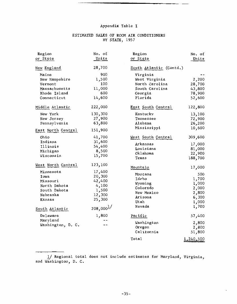
Appendix Table I

ESTIMATED SALES OF ROOM AIR CONDITIONERS BY STATE, 1957

Region No. of Region or State Units or State

No. of Units

New England 28,700

900 1,500

100 11,000

600 14,600

222,000

130,300 27,900 63,800

151,900

41,700 31,600 54,400 8,500 15,700

123,100

17,400 20,300 42,400 4,100 1,500

12,300 25,300

208,00011

1,800

South Atlantic (Contd.)

2,200 28,700 43,800 78,900 52,600

122,800

13,100 72,900 26,200

309,600

81,000

188,700

17,000

2,800

1,000

57,400

2,800 51,800

1,240,500

Maine New Hampshire Vermont Massachusetts Rhode Island Connecticut

Middle Atlantic

Virginia West Virginia North Carolina South Carolina Georgia Florida

East South Central

New York New Jersey Pennsylvania

East North Central 10,600

Kentucky Tennessee Alabama Mississippi

West South Central Ohio Indiana Illinois Michigan Wisconsin

West North Central

17,000

22,900

Arkansas A Louisiana Oklahoma Texas

Mountain Minnesota Iowa Missouri North Dakota South Dakota Nebraska Kansas

South Atlantic

500 1,700 1,000 2,000

6,300

1,700

Montana M Ideho Wyoming Colorado New Mexico Arizona A Utah Nevada

Pacific Delaware Maryland Washington, D. C. 2,800

Washington Oregon Calitornia

Total

1/ Regional total does not include estimates for Maryland, Virginia, and Washington, D. C.

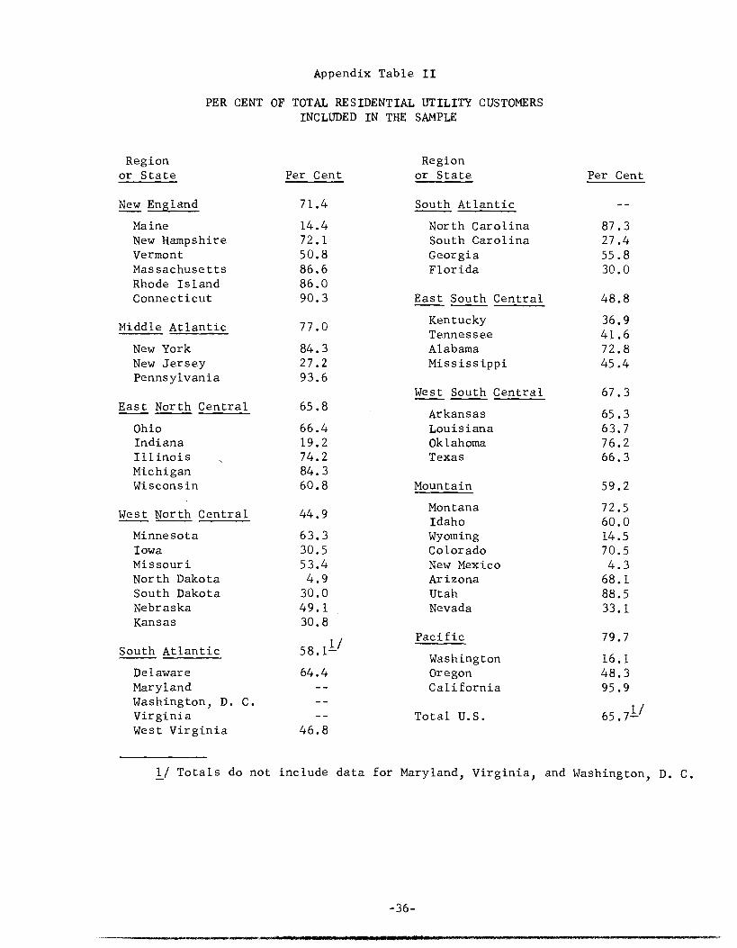
Appendix Table II

PER CENT OF TOTAL RESIDENTIAL UTILITY CUSTOMERS INCLUDED IN THE SAMPLE

Region or State Per Cent

Region or State Per Cent

New England 71.4 South Atlantic

Maine 14.4 North Carolina 87.3 New Hampshire 72.1 South Carolina 27.4 Vermont 50.8 Georgia 55.8 Massachusetts 86.6 Florida 30.0 Rhode Island 86.0 Connecticut 90.3 East South Central 48.8

Middle Atlantic 77.0 Kentucky Tennessee

36.9 41.6

New York 84.3 Alabama 72.8 New Jersey 27.2 Mississippi 45.4 Pennsylvania 93.6

West South Central 67.3 East North Central 65.8

Arkansas 65.3 Ohio 66.4 Louisiana 63.7 Indiana 19.2 Oklahoma 76.2 Illinois 74.2 Texas 66.3 Michigan 84.3 Wisconsin 60.8 Mountain 59.2

West North Central 44.9 Montana Idaho

72.5 60.0

Minnesota 63.3 Wyoming 14.5 Iowa 30.5 Colorado 70.5 Missouri 53.4 New Mexico 4.3 North Dakota 4.9 Arizona 68.1 South Dakota 30.0 Utah 88.5 Nebraska 49.1 Nevada 33.1 Kansas 30.8

Pacific 79.7 South Atlantic 58.11/

Washington 16.1 Delaware 64.4 Oregon 48.3 Maryland California 95.9 Washington, D. C. Virginia Total U.S. 65.711 West Virginia 46.8

1/ Totals do not include data for Maryland, Virginia, and Washington, D. C. ....

Appendix II

FORECAST METHODOLOGY

An arithmetic graph of production data from 1947 to 1957 reveals quite

clearly that after the tremendous expansion of output from 1952 to 1954, the

industry was faced with an inventory problem. The recessions of 1954 and

late 1957 contributed to this problem and incidentally lend an element of

conservatism to the forecasts.

To overcome the effects of inventory adjustments, two-year moving aver-

ages of the production data were used as the basis of the forecasts. This ad-

justment of the-data also has a tendency to bring production more in line

with actual sales, so that although technically production is being forecast,

the results should be reasonably close to sales.

The Modified Exponential Method

After the adjustment, the data still show no obvious tendency to regular-

ity of growth (Figure 2). It will be noted that the logarithmic graph passes

through three cycles of these orders of magnitude: 101, 10

2, and 10

3. This

characteristic can obscure regularity in growth simply through differences in

magnitude of the data. A transformation was applied to reveal any such hidden

tendency.

To each production datum, a constant factor (K) of 5471/

was added. This

transformation has the effect of giving more emphasis to the increases from

year to year. The transformed data is graphed in Figure 3.

By a linear extrapolation of the last section of the curve in Figure 3,

and subtracting K, the first forecast of 2,250,000 units in 1959-60 was

obtained. For short term forecasts this method, termed "fitting a modified

exponential curve," may be quite satisfactory.

1/ Derived by grouping the data into three parts: 1947-48, 1948-49, 1949-50, 1950-51; 1950-51, 1951-52, 1952-53, 1953-54; 1953-54, 1954-55, 1955-56, 1956-57. Summing and averaging, the mean of part 1 (designated as M1 ) is 124.75, M2 = 609.25, M3 = 1,443.00. Then,

2 K 2 -1 M3 1 + M3 ) - 2Y12I = 547.

The K is added algebraically, i.e., a negative K would be subtracted.

Correlation Method

As a check on the results of the first method, U.S. total production

and personal income were tested for degree of correlation for the purpose of

using an income forecast as a basis for a production forecast. The advantage

of such a method is that the wide range of factors determining income provides

a much more stable base, and consequently greater reliability, than assump-

tions that might be made for the future of a particular product.

Two adjustments were made in the income data. The data were deflated

to reflect price level changes, and converted to a two-year moving average

series to increase the time-comparability of the two sets of data.

By least squares regression the following equations were specified, with

the indicated correlation coefficients:

P = -4,313 + 21.22158(Y) (r = 0.96)

Y = 193.85 + 9.7212(T) (r = 0.99)

where P = Production, Y = Income, T = Time, origin at 1947-48.

The forecast obtained for 1959-60 is 2,280,000 units, which closely agrees

with the former forecast of 2,250,000 units.