MODEL-BASED CONTROL AND PILOT CUEING TECHNIQUES FORAUTOROTATION MANEUVERS

A DissertationPresented to

The Academic Faculty

By

Brian Eberle

In Partial Fulfillmentof the Requirements for the Degree

Doctor of Philosophy in theSchool of Mechanical Engineering

Georgia Institute of Technology

December 2020

c© Brian Eberle 2020

MODEL-BASED CONTROL AND PILOT CUEING TECHNIQUES FORAUTOROTATION MANEUVERS

Thesis committee:

Dr. Jonathan Rogers, ChairSchool of Aerospace EngineeringGeorgia Institute of Technology

Dr. Anirban MazumdarSchool of Mechanical EngineeringGeorgia Institute of Technology

Dr. Jun UedaSchool of Mechanical EngineeringGeorgia Institute of Technology

Dr. J.V.R. PrasadSchool of Aerospace EngineeringGeorgia Institute of Technology

Dr. Michael JumpMechanical, Materials & AerospaceEngineeringUniversity of Liverpool

Date approved: October 2, 2020

I have no special talent. I am only passionately curious.

Albert Einstein

For Gwen, Paul, Mom and Dad.

ACKNOWLEDGMENTS

I would first like to thank my advisor Dr. Jonathan Rogers for his guidance and support

as I completed this work. Dr. Rogers’ technical prowess and scrutiny encouraged me to

always hold my work to a higher standard. He works hard to create a productive research

environment that is free from unnecessary distraction or stress. This environment along

with his judicious advice have been integral to my development as an engineer and person.

I would also like to thank the Vertical Lift Research Center of Excellence (VLRCOE)

and the Vertical Flight Society (VFS) for supporting my time as a graduate student and

providing constructive platforms to share my work. I want to thank the members of my

committee: Dr. Mike Jump, Dr. Anirban Mazumdar, Dr. J.V.R. Prasad, and Dr. Jun Ueda

for their time in helping guide and improve this research.

I want to thank my fellow members of Dr. Rogers’ research group: Jared Elinger, Kevin

Webb, Joey Meyers, Dakota Musso, Jonathan Warner, Andrew Leonard, Umberto Saetti,

Geordan Gutow, Sam Kemp, and Adam Garlow. Together we made a healthy, fun, and

constructive workplace that made my time in grad school more enjoyable.

I need to thank my mom and dad for their unending support. My mom fostered an

interest in aviation by taking me to every airshow we could make, starting at a young age.

Her example as an airline pilot showed me that you can achieve anything if you pursue

your passions. My dad impressed on me by example the importance of education and hard

work. I also want to thank Paul for his constant help in achieving this goal and all others

throughout my life. I want to thank Gwen for her love and kindness over the last five years.

Without daily encouragement from her and my family, this certainly would not have been

possible.

Finally, I want to thank all my professors, teachers, friends, and family because nothing

is accomplished alone. This would not have been possible without the help of countless

people.

v

TABLE OF CONTENTS

Acknowledgments . . . . . . . . . . . . . . . . . . . . . . . . . . . . . . . . . . . v

List of Tables . . . . . . . . . . . . . . . . . . . . . . . . . . . . . . . . . . . . . . ix

List of Figures . . . . . . . . . . . . . . . . . . . . . . . . . . . . . . . . . . . . . x

Summary . . . . . . . . . . . . . . . . . . . . . . . . . . . . . . . . . . . . . . . . xiii

Chapter 1: Introduction and Background . . . . . . . . . . . . . . . . . . . . . . 1

1.1 Problem Motivation . . . . . . . . . . . . . . . . . . . . . . . . . . . . . . 1

1.1.1 Landing Point Reachability During Descent . . . . . . . . . . . . . 4

1.2 Work Overview . . . . . . . . . . . . . . . . . . . . . . . . . . . . . . . . 5

1.2.1 Dissertation Outline . . . . . . . . . . . . . . . . . . . . . . . . . . 6

Chapter 2: Landing Point Tracking and Trajectory Feasibility Determination . 7

2.1 Landing Point Tracking Algorithm . . . . . . . . . . . . . . . . . . . . . . 7

2.1.1 Mathematical Formulation . . . . . . . . . . . . . . . . . . . . . . 9

2.2 Trajectory Feasibility Evaluation . . . . . . . . . . . . . . . . . . . . . . . 13

2.2.1 Reduced-Order Vehicle Dynamics . . . . . . . . . . . . . . . . . . 14

2.3 Results . . . . . . . . . . . . . . . . . . . . . . . . . . . . . . . . . . . . . 19

2.3.1 Landing Point Tracking Example Results . . . . . . . . . . . . . . 19

vi

2.3.2 Landing Point Tracking Trade Studies . . . . . . . . . . . . . . . . 26

2.3.3 Low-order Dynamic Model Validation . . . . . . . . . . . . . . . . 36

2.3.4 Feasibility Evaluation Algorithm Example Case . . . . . . . . . . . 39

2.3.5 Feasibility Evaluation Algorithm Robustness Studies . . . . . . . . 43

2.4 Chapter Summary . . . . . . . . . . . . . . . . . . . . . . . . . . . . . . . 50

Chapter 3: Model Predictive Control . . . . . . . . . . . . . . . . . . . . . . . . 52

3.1 Chapter Motivation . . . . . . . . . . . . . . . . . . . . . . . . . . . . . . 52

3.2 Nonlinear Model Predictive Control Law Formulation . . . . . . . . . . . . 52

3.2.1 Mathematical Formulation . . . . . . . . . . . . . . . . . . . . . . 53

3.2.2 Reference Trajectory Generation . . . . . . . . . . . . . . . . . . . 56

3.2.3 State-Dependent Rotor Speed Penalty . . . . . . . . . . . . . . . . 57

3.2.4 Control Implementation . . . . . . . . . . . . . . . . . . . . . . . . 58

3.3 Results . . . . . . . . . . . . . . . . . . . . . . . . . . . . . . . . . . . . . 59

3.3.1 Simulation Model . . . . . . . . . . . . . . . . . . . . . . . . . . . 59

3.3.2 Example Trajectories . . . . . . . . . . . . . . . . . . . . . . . . . 61

3.3.3 Trade Studies . . . . . . . . . . . . . . . . . . . . . . . . . . . . . 65

3.3.4 Monte Carlo Analyses . . . . . . . . . . . . . . . . . . . . . . . . 67

Chapter 4: Landing Point Reachability . . . . . . . . . . . . . . . . . . . . . . . 90

4.1 Chapter Motivation . . . . . . . . . . . . . . . . . . . . . . . . . . . . . . 90

4.2 Reachability Algorithm . . . . . . . . . . . . . . . . . . . . . . . . . . . . 90

4.2.1 Algorithm Overview . . . . . . . . . . . . . . . . . . . . . . . . . 90

4.2.2 Descent Rate Study . . . . . . . . . . . . . . . . . . . . . . . . . . 92

vii

4.2.3 Terrain Elevation Considerations . . . . . . . . . . . . . . . . . . . 95

4.3 Head Up Display Implementation . . . . . . . . . . . . . . . . . . . . . . . 97

4.4 Limited Piloted Studies . . . . . . . . . . . . . . . . . . . . . . . . . . . . 98

Chapter 5: Conclusion . . . . . . . . . . . . . . . . . . . . . . . . . . . . . . . . 102

5.1 Contributions . . . . . . . . . . . . . . . . . . . . . . . . . . . . . . . . . 102

5.2 Recommended Future Work . . . . . . . . . . . . . . . . . . . . . . . . . 103

5.2.1 Landing Point Tracking and Reachability in Flare . . . . . . . . . . 103

5.2.2 Nonlinear Model Predictive Control . . . . . . . . . . . . . . . . . 103

5.2.3 Landing Site Reachability and Pilot Cueing in Descent . . . . . . . 104

Appendices . . . . . . . . . . . . . . . . . . . . . . . . . . . . . . . . . . . . . . . 106

Appendix A: Nonlinear Model Predictive Control Equations . . . . . . . . . . . 107

Appendix B: OH-58C Autorotation Data . . . . . . . . . . . . . . . . . . . . . 110

References . . . . . . . . . . . . . . . . . . . . . . . . . . . . . . . . . . . . . . . 111

Vita . . . . . . . . . . . . . . . . . . . . . . . . . . . . . . . . . . . . . . . . . . . 116

viii

LIST OF TABLES

2.1 Criteria Used to Determine the Success of an Autorotative Landing. . . . . 33

2.2 Reduced-Order Helicopter Parameters. . . . . . . . . . . . . . . . . . . . . 37

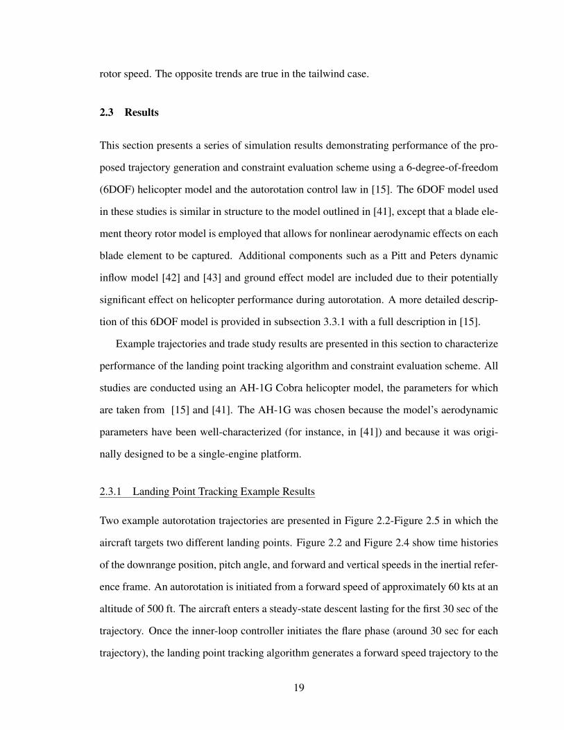
2.3 State Bounds Determining Feasible Landing Point Limits. . . . . . . . . . . 40

2.4 Nominal and Off-Nominal Flare Entry Conditions. . . . . . . . . . . . . . 44

3.1 Reduced Order Model, Trajectory, and Controller Parameters . . . . . . . . 68

3.2 Criteria Used to Determine the Success of an Autorotative Landing (Re-stated). . . . . . . . . . . . . . . . . . . . . . . . . . . . . . . . . . . . . . 70

ix

LIST OF FIGURES

1.1 Autorotation Sequence. . . . . . . . . . . . . . . . . . . . . . . . . . . . . 3

2.1 Landing Point Tracking Algorithm and Feasibility Evaluation AlgorithmIntegrated with Autorotation Controller from [15]. . . . . . . . . . . . . . . 8

2.2 Landing Point Tracking Algorithm Example Trajectory 1. . . . . . . . . . . 21

2.3 Landing Point Tracking Algorithm Example Trajectory 1 in Flare. . . . . . 22

2.4 Landing Point Tracking Algorithm Example Trajectory 2. . . . . . . . . . . 23

2.5 Landing Point Tracking Algorithm Example Trajectory 2 in Flare. . . . . . 24

2.6 Altitude vs Distance From Flare Entry for Landing Point Tracking TradeStudy. . . . . . . . . . . . . . . . . . . . . . . . . . . . . . . . . . . . . . 27

2.7 Pitch Angle vs Time for Landing Point Tracking Trade Study. . . . . . . . . 28

2.8 Forward Speed vs Time for Landing Point Tracking Trade Study. . . . . . . 29

2.9 Landing Distance Error vs Target Distance for Landing Point TrackingTrade Study. . . . . . . . . . . . . . . . . . . . . . . . . . . . . . . . . . . 31

2.10 State Limits for Landing Point Tracking Trade Study. . . . . . . . . . . . . 32

2.11 Landing Distance Error vs Steady Wind Speed for Landing Point TrackingMonte Carlo Study. . . . . . . . . . . . . . . . . . . . . . . . . . . . . . . 34

2.12 Landing Distance Error vs Vehicle Gross Weight for Landing Point Track-ing Monte Carlo Study. . . . . . . . . . . . . . . . . . . . . . . . . . . . . 35

2.13 Forward Speed and Vertical Speed Comparisons Between Reduced-Orderand 6DOF Models. . . . . . . . . . . . . . . . . . . . . . . . . . . . . . . 37

x

2.14 Pitch Angle and Rotor Speed Comparisons Between Reduced-Order and6DOF Models. . . . . . . . . . . . . . . . . . . . . . . . . . . . . . . . . . 38

2.15 Feasible Landing Point Evaluation Algorithm Example Case, Initial Solution. 41

2.16 Feasible Landing Point Evaluation Algorithm Example Case, Updated asManeuver Progresses. . . . . . . . . . . . . . . . . . . . . . . . . . . . . . 42

2.17 Feasible Landing Point Evaluation, First Off-Nominal Flare Entry Condition. 45

2.18 Feasible Landing Point Evaluation, Second Off-Nominal Flare Entry Con-dition. . . . . . . . . . . . . . . . . . . . . . . . . . . . . . . . . . . . . . 46

2.19 Feasible Landing Point Evaluation, 9kt Headwind Case. . . . . . . . . . . . 48

2.20 Feasible Landing Point Evaluation, 6kt Tailwind Case. . . . . . . . . . . . 49

3.1 State-Dependent Rotor Speed Tracking Penalty. . . . . . . . . . . . . . . . 58

3.2 MPC Implementation with Helicopter Simulator. . . . . . . . . . . . . . . 59

3.3 Example Case 1 Output States: Targeting 550 ft downrange. . . . . . . . . 72

3.4 Example Case 1 Controls: Targeting 550 ft downrange. . . . . . . . . . . . 73

3.5 Example Case 2 Output States: Targeting 1,010 ft downrange. . . . . . . . 74

3.6 Example Case 2 Controls: Targeting 1,010 ft downrange. . . . . . . . . . . 75

3.7 Example Case 3 Output States: Targeting 775 ft downrange. . . . . . . . . 76

3.8 Example Case 3 Controls: Targeting 775 ft downrange. . . . . . . . . . . . 77

3.9 Comparison of Number of Taylor Series Terms with Constant Time Horizon. 78

3.10 Comparison of Number of Taylor Series Terms with Constant Time Hori-zon Cont. . . . . . . . . . . . . . . . . . . . . . . . . . . . . . . . . . . . 79

3.11 Comparison of Number of Taylor Series Terms with Varied Time Horizon. . 80

3.12 Comparison of Number of Taylor Series Terms with Varied Time HorizonCont. . . . . . . . . . . . . . . . . . . . . . . . . . . . . . . . . . . . . . . 81

xi

3.13 Landing Point Tracking Trade Study PID Comparison Metrics, Gross Weight8,300lbs. . . . . . . . . . . . . . . . . . . . . . . . . . . . . . . . . . . . . 82

3.14 Landing Point Tracking Trade Study PID Comparison Metrics, Gross Weight8,300lbs Cont. . . . . . . . . . . . . . . . . . . . . . . . . . . . . . . . . . 83

3.15 Landing Point Tracking Trade Study PID Comparison Metrics, Gross Weight10,000lbs. . . . . . . . . . . . . . . . . . . . . . . . . . . . . . . . . . . . 84

3.16 Landing Point Tracking Trade Study PID Comparison Metrics, Gross Weight10,000lbs Cont. . . . . . . . . . . . . . . . . . . . . . . . . . . . . . . . . 85

3.17 Landing Point Tracking Trade Study PID Comparison Metrics, Gross Weight7,000lbs. . . . . . . . . . . . . . . . . . . . . . . . . . . . . . . . . . . . . 86

3.18 Landing Point Tracking Trade Study PID Comparison Metrics, Gross Weight7,000lbs Cont. . . . . . . . . . . . . . . . . . . . . . . . . . . . . . . . . . 87

3.19 Gross Weight and Target Landing Point Variation Monte Carlo Study. . . . 88

3.20 Gross Weight and Target Landing Point Variation Monte Carlo Study Cont. 88

3.21 Height-Velocity Diagram Autorotation Entry Condition Monte Carlo Study. 89

4.1 Example Reachable Footprints as Vehicle Descends . . . . . . . . . . . . . 93

4.2 Reachable Footprint with 015o Heading, 1000ft. altitude and a 6kt WesterlyWind . . . . . . . . . . . . . . . . . . . . . . . . . . . . . . . . . . . . . . 94

4.3 Results of Descent Rate Study . . . . . . . . . . . . . . . . . . . . . . . . 95

4.4 Reachable Footprint at Varied Bank Angles (800 ft. AGL, 100kts) . . . . . 96

4.5 Reachable Footprint Over Varied Terrain . . . . . . . . . . . . . . . . . . . 97

4.6 Screenshot Reachability Cue Implemented at University of Liverpool. . . . 98

4.7 Screenshot of Reachability Cue Implemented at Georgia Tech. . . . . . . . 99

4.8 Piloted Trajectories Overlaid with Reachable Prediction Markers . . . . . . 100

B.1 Flight Test Data From Piloted Autorotation in OH-58C . . . . . . . . . . . 110

xii

SUMMARY

Autorotation maneuvers are performed by pilots to safely land after an engine failure in

a helicopter. These maneuvers are difficult due to the small window for successful timing,

the wide range of possible entry conditions, and the potentially catastrophic consequences

of a mistake. This work focuses on automation of the autorotation maneuver and the de-

velopment of cues to aid in piloted autorotations. Specifically, this work is broken into

three main categories: landing point tracking and reachability determination near landing,

model predictive control through touchdown, and a landing site reachability determination

algorithm and pilot cue. The landing point tracking scheme utilizes a biomimetic strategy

called tau theory to generate sub-optimal trajectories nearly instantaneously. A point-mass

physical model of the helicopter is then applied to predict states and control along an input

trajectory. These predicted states can be used to determine the feasibility of the given tra-

jectory. A set of candidate trajectories can be generated and evaluated using these methods

to find a sub-optimal set of reachable landing points. This set of landing points can be used

to cue a pilot to aid with landing point selection. The Nonlinear Model Predictive Control

(NMPC) method proposed here offers several potential benefits over existing control meth-

ods including the capability to intelligently balance state constraints on three outputs using

only two control inputs. This multi-input multi-output NMPC method solves for the op-

timal control inputs in closed form using the same point-mass helicopter model employed

above. This ensures deterministic runtime and enables real-time execution, a necessities for

aerial vehicles. An algorithm to determine the reachable landing points in descent phase

is presented along with implementation of two Head Up Displays driven by the algorithm.

Limited piloted studies are presented to evaluate the usefulness of such a cue.

xiii

CHAPTER 1

INTRODUCTION AND BACKGROUND

1.1 Problem Motivation

Autorotation is a complex flight maneuver that requires the pilot to perform several tasks

precisely in a carefully-timed manner. While it is possible that visual, haptic, or other

specially-designed cues may reduce pilot workload in autorotation or increase the likeli-

hood of a successful landing, there has been extremely limited success in fielding cue-

ing systems for autorotation to date. At the same time, as interest in autonomous and

optionally-piloted rotorcraft continues to grow, there is an increasing need for autonomous

control algorithms that can successfully recover an aircraft in the case of in-flight engine or

transmission failures. For both pilot cueing systems and autonomous control algorithms,

certification demands will likely dictate that the underlying algorithms execute with deter-

ministic runtime performance and avoid the use of highly-calibrated models, which may be

difficult to obtain for many aircraft.

Autonomous control and pilot cueing in autorotation has been the focus of a consider-

able amount of prior research. Johnson [1] conducted some of the first investigations into

control of a helicopter in autorotation. This work applied optimal control theory to a point

mass model of the helicopter dynamics to generate optimal state and control time histories

given a set of boundary conditions. Lee et al. [2] further developed this approach to show

that the avoid region of the height-velocity diagram could be reduced if the maneuver can

be automated through closed-loop control. The proposed control scheme was implemented

offline, however, and was intended for use during vehicle design rather than for online

control. Similar analyses have been conducted for tiltrotor aircraft by Carlson and Zhao

[3]. Abbeel et al. [4] applied a reinforcement learning technique to generate controller

1

inputs similar to those recorded during piloted trajectories. Control law performance was

validated by executing autonomous autorotations on a hobby-sized helicopter.

Recently, Grande et al. [5, 6, 7] utilized the low-order dynamic model of a helicopter in

autorotation developed by Johnson [1] to calculate the backward reachable set of safe flare

entry states. The authors used an iterative scheme to solve for optimal flare trajectories,

from which a set of safe flare entry states could be established. The trajectory generator

proposed in this approach does not exhibit deterministic runtime performance due to the

underlying iterative optimization, and thus might not provide a suitable approach to online

trajectory generation in an autorotative flare. Yomchinda et al. [8] combined the flare

trajectory generating functionality from [6] with an optimal path planning algorithm during

autorotation entry and descent phases (See Figure 1.1).

Nonlinear model predictive control (NMPC) during autorotation has also been inves-

tigated. Dalamagkidis et al. [9] used NMPC and a recurrent neural network to generate

optimal trajectories using a simple dynamic helicopter model in vertical autorotation. Wil-

son and Prazenica [10] applied NMPC to a tilt rotor using a medium fidelity model of the

dynamics to determine the control inputs and used a neural network to minimize the cost

function. A high-fidelity model is used for validation. While this approach shows promise

in stabilizing the higher fidelity simulation and meeting applied constraints, the conver-

gence of the optimization problem appears to be parameter dependent and may preclude

its use in online applications. MPC of helicopters in powered flight has been studied for

applications such as shipboard landings [11, 12] and could yield practical benefits during

autorotation due to the increased number of competing state constraints.

The autorotation control problem can be broken into two distinct segments: steady de-

scent and autorotative flare as depicted in Figure 1.1. The flare is highly dynamic and

complex compared to the descent and is generally considered to be the most difficult seg-

ment to automate due to its high dimensionality and numerous state constraints [5]. Thus,

the primary control focus of this work is on the flare portion of the maneuver. Several prior

2

Figure 1.1: Autorotation Sequence.

investigations into autorotative flare trajectory generation use an optimal control approach

that seeks to balance control effort against the need to obtain a desired state at touchdown,

while in some cases meeting constraints on states and control [1, 2, 3, 5, 7, 6, 8, 13, 14].

However, due to the nonlinearity of the system dynamics, these optimal trajectories must

be obtained through iterative optimization schemes which lack deterministic runtime per-

formance and convergence guarantees. To leverage such an approach for on-board control,

a database of trajectories would need to be developed offline for every state, wind, and

weight condition that could be encountered at flare entry. Such a database could be very

large and may lack robustness to modeling errors or other systematic disturbances.

A different approach may be taken in which the optimality of the trajectory is sacrificed

in order to obtain deterministic runtime performance and the ability to update the control

solution in real-time as the maneuver evolves. Along these lines, Sunberg et al. [15, 16] de-

veloped a real-time expert control system that was shown through simulation to be capable

of successfully landing a helicopter from a wide range of maneuver entry conditions. Two

noted shortcomings of this control scheme are its inability to provide guidance to a specific

desired landing point on the ground and its lack of conditioning on rotor speed constraints.

The goal of the work presented here is to address these shortcomings, while maintaining

the deterministic runtime performance and real-time execution capabilities of this previous

line of work.

3

A key aspect of the autorotation controller developed in [15, 16] is its utilization of the

predicted time-to-contact with the ground, which is used to shape the flare trajectory and

trigger transitions between control phases. This creates a bridge with prior work in optical

tau theory which has been studied extensively by Padfield et al. [17, 18, 19, 20, 21, 22].

In an aerospace controls context, tau theory or time-to-contact theory postulates that pilots

guide an aircraft in proximity to the ground by detecting gap closure rates and comparing

them with so-called intrinsic or extrinsic tau guides, where tau denotes the time-to contact

with an obstacle. Parameterization by optical tau has been shown to not only simplify

control schemes associated with various aircraft maneuvers, but also to mitigate the effects

of unstable vehicle modes while avoiding dynamic inversion [19]. There is significant

evidence obtained from analysis of flight data that pilots use a guidance strategy based on

optical tau in fixed-wing aircraft flare [17] and other common maneuvers [19, 21]. Tau

theory has also been used as the basis in various respects for powered helicopter landings,

flight controllers, pilot modeling, and guidance methods [20, 23, 24].

1.1.1 Landing Point Reachability During Descent

Rapid and effective selection of a landing site is critical to the success of an autorotation

maneuver. An otherwise safe landing in an unsuitable location could be hazardous. Pilot

selection of a landing site may be hindered by a lack of familiarity with the terrain or by

meteorological conditions at the time of power loss. Landing site selection and approach

are accomplished during the descent phase of Figure 1.1, so an additional portion of work

is dedicated to reachability during this phase. Head Up or Head Down Displays could

potentially enable faster and more effective landing point selection during autorotation.

Such cues on a Head Down Display could prove particularly useful in degraded visual

environments (DVE). For the purposes of this work the term ”reachability” is taken to

mean landing site reachability rather than any more formal definition.

Considerable work has been done investigating pilot cues during autorotation [13, 25,

4

14, 26, 27, 28, 29], although these cues focus largely on aiding pilot control action rather

than landing site decision making and few if any of the approaches have been fielded to

date. While a dynamic model is likely needed to evaluate the reachability in flare, a purely

kinematic approach is presented for finding the reachable footprint in the descent phase.

This is valid because the dynamics are much more steady in the descent phase than in

the flare. Landing site reachability during the descent phase is also important because the

majority of the positioning towards the target landing area is conducted during the descent

phase.

Landing site reachability determination and cueing after engine failure have been stud-

ied more extensively in fixed-wing aircraft [30, 31, 32, 33, 34, 35, 36] and have been shown

to reduce pilot workload [32]. This shows the potential for such technology in rotorcraft;

however, a novel approach must be taken given the dynamics unique to helicopters.

1.2 Work Overview

This dissertation first extends the prior work in [15, 16, 26] by introducing a rapid trajec-

tory generation scheme for autorotative flare that enables a pilot or autonomous controller

to track a desired landing point. The algorithm leverages optical tau theory to generate

trajectory solutions quickly, sacrificing optimality for guaranteed runtime. The dynamic

feasibility of the resulting trajectory is evaluated through the use of the low order model

of the helicopter in autorotation proposed in [1]. This constraint evaluation involves a re-

verse solution process in which the known velocities and accelerations are used to solve

for the needed forces and rotor states, which are then compared against known operational

constraints. When coupled to the control law in [15], the resulting algorithm is capable of

autonomous autorotation to a desired landing point. It can furthermore be used to provide a

pilot or landing site selection algorithm with bounds on reachable landing locations in the

flare.

While the aforementioned determination of the dynamically feasible landing points is

5

beneficial, incorporating rotor speed management into the control law may be a more direct

solution to the problem. Slegers et al. [37] outlines a nonlinear model predictive control

technique for generic flight vehicles. This multi-input, multi-output approach is well suited

for aerial vehicles because it solves for optimal control derivatives in closed form given

a model of the system to be controlled and a desired trajectory for each of the output

states. Such a control approach is applicable to autorotation particularly during the flare and

landing phases. This dissertation presents the formulation of a nonlinear model predictive

controller for autorotation using the form presented in [37] and the helicopter model derived

in [1]. A state-dependent rotor speed tracking penalty is presented, and the algorithm is

applied in simulation using example reference trajectories for forward and vertical speed in

autorotative flare. Simulation results from a medium-fidelity, six-degree-of-freedom model

are reported.

Lastly, this work outlines the development of an approach for determining the reachable

landing point footprint during the descent phase. Example footprints are shown for various

altitudes, wind conditions, and terrain elevation maps. A preliminary Head Up Display

has been implemented in multiple simulator environments, and results of limited piloted

studies are presented.

1.2.1 Dissertation Outline

The dissertation proceeds as follows: Chapter 2 shows the development and results of the

landing point tracking trajectory generation and the feasibility determination schemes for

flare. Chapter 3 shows the formulation and simulation results of the Nonlinear Model Pre-

dictive Control approach. Chapter 4 covers the landing footprint determination algorithm

for the descent phase as well as its implementation as a Head Up Display and the results of

limited piloted studies. Finally, Chapter 5 summarizes the main contributions of the work

and suggests avenues for future work.

6

CHAPTER 2

LANDING POINT TRACKING AND TRAJECTORY FEASIBILITY

DETERMINATION

2.1 Landing Point Tracking Algorithm

For the purposes of this paper, landing point tracking refers to the ability to generate a

forward speed deceleration trajectory that enables the helicopter to reach the target landing

point at the time of touchdown. A key design constraint that leads to the formulation of

the presented algorithm is that it must have deterministic (and preferably rapid) runtime

performance. This enables feedback planning which provides some measure of robustness

to tracking error, outside disturbances, and uncertainties in winds and vehicle dynamics.

Deterministic runtime performance is also a likely pre-requisite for eventual certification.

In addition to this design constraint, several other key assumptions underlie the work

in this chapter. First, the algorithm presented here considers only the flare segment of au-

torotation, which is differentiated from the descent portion by the initiation of deceleration

in the forward and vertical directions, as shown in Figure 1.1. It is assumed that turns

will be avoided in an autorotative flare, and thus the algorithm considers planar motion of

the aircraft only (i.e., no lateral motion is considered). As a result, for fully autonomous

autorotation the trajectory generator described here would need to be used in conjunction

with a separate trajectory planning scheme in steady-state (for instance from [8]) to ensure

the vehicle approaches the landing region effectively.

A second key assumption is that the trajectory generated through the approach outlined

here is tracked by either a pilot or inner-loop autorotation controller such as that described

in [15] or in Chapter 3 of this work. Figure 2.1 shows a block diagram of a fully-integrated

autorotation flare controller in which the trajectory generator is coupled to the inner-loop

7

Figure 2.1: Landing Point Tracking Algorithm and Feasibility Evaluation Algorithm Inte-grated with Autorotation Controller from [15].

controller from [15]. Given the vehicle state at a given time and a desired landing point, the

landing point tracking algorithm creates a commanded forward speed profile ucom. This

is provided to the constraint evaluation scheme (dashed box in Figure 2.1), which predicts

the rotor speed and vehicle pitch angle time histories (Ω(t) and θ(t), respectively) over

the course of the flare trajectory. If these predictions exceed threshold limits, the landing

point is considered outside the reachable set and is rejected. Otherwise, the forward speed

trajectory ucom is sent to the inner-loop controller for tracking in the flare. The two main

blocks at the bottom of Figure 2.1 are described in this chapter. The inner-loop controller at

the top of Figure 2.1 may be replaced with a pilot or alternative autorotation scheme, such

as that presented in Chapter 3.

A final assumption underlying the work of this chapter is that the inner-loop autorota-

tion control algorithm has an independent mechanism of controlling motion in the vertical

channel. For instance, in [15], collective control is driven strictly based on estimates of

time-to-ground-contact using a simple control law, but a forward speed trajectory is re-

quired for tracking. The algorithm provided here is designed to produce a forward speed

8

trajectory only, and it is assumed that the inner-loop algorithm or the pilot controls the

vertical speed through through an independent control scheme.

2.1.1 Mathematical Formulation

Define the horizontal distance from the vehicle to the target landing point as x and the

altitude above ground of the helicopter as h. To arrive at the desired landing point at the

moment of touchdown, these two gaps must be closed simultaneously in the same amount

of time. Following tau theory terminology, τx is the instantaneous time to contact defined

as,

τx =x

x(2.1)

and is the instantaneous estimate of the gap closure time if the velocity is held constant.

The time derivative of this quantity is given as,

τx = 1− xx

x2(2.2)

Tau theory literature [17, 18, 19, 20] suggests that pilots commonly generate guidance

commands that maintain a constant rate of change in τ during gap closure. Thus, the

constant parameter k is introduced such that,

k = 1− τx =xx

x2(2.3)

where the bounds k ∈ [−1, 1] are typically enforced. This differential equation—a func-

tion of position, forward speed, and forward acceleration—parameterizes the downrange

position of the helicopter by k. The second-order ODE in Equation 2.3 can be written as

an initial value problem as follows,

x = u (2.4)

9

u =ku2

x(2.5)

x(0) = xi (2.6)

u(0) = ui (2.7)

where xi and ui denote the position and forward (ground) speed of the helicopter at the

time trajectory planning is initiated. Closed-form solutions for Equation 2.4-Equation 2.7,

derived by Lee [38], are given by,

x(t) = xi

[1− (k − 1)uit

xi

]− 1k−1

(2.8)

u(t) = ui

[1− (k − 1)uit

xi

]−1− 1k−1

(2.9)

Equation 2.8 and Equation 2.9 provide a closed-form trajectory solution for x and u

parameterized by k. Let the estimated time until the helicopter reaches the ground be given

by T . Then the goal of the trajectory generator is to solve for k such that x(T ) = 0. This

can be accomplished by solving the following nonlinear equation,

xi

[1− (k − 1)uiT

xi

]− 1k−1

= xTH ≈ 0 (2.10)

where k is the only unknown and xTH is a small threshold value close to zero that is

needed to avoid a singularity when the right-hand-side of Equation 2.10 is exactly zero.

Equation 2.10 is a one-dimensional nonlinear root finding problem. Although it is possible

to use an iterative root finding method such as Newton-Raphson to solve for k, this leads

to non-deterministic runtime performance and is thus undesirable. In practice however, the

10

domain limitation k ∈ [−1, 1] can be used to create a one-dimensional mesh of candidate

solutions kj , j = 1, ..., J . Each candidate solution can be used to evaluate Equation 2.10,

and the ”optimal” value kopt selected from the candidate set is that which yields a final

position (on the right-hand-side of Equation 2.10) closest to xTH . Note that evaluation of

Equation 2.10 with a candidate k value is extremely fast, meaning that the resolution of

the mesh of candidate k solutions can be quite high. While the selected kopt is mathemati-

cally suboptimal, in practice the value is close enough to the actual optimal value with the

added benefit that it can be determined quite rapidly in a known amount of computation

time. To verify that the degree of suboptimality resulting from this solution approach is

small enough to be negligible, a comparison was performed between various trajectory so-

lutions obtained using a discretized mesh of k values with resolution 0.01 (200 total points)

with the converged solutions from a Newton-Raphson solver with maximum relative error

tolerance of 0.001. The solutions matched to at least two decimal places and often even

more closely. The approximate solutions are therefore close enough in practice to the true

optimal value, and any small reduction in optimality is likely to cause negligible loss of

performance.

Substituting kopt into Equation 2.9 yields

ucom(t) = ui

[1− (kopt − 1)uit

xi

]−1− 1kopt−1

(2.11)

which is the commanded velocity trajectory for the flare maneuver (or the remainder of it,

depending on when planning is performed). The trajectory ucom may be provided to an

inner-loop velocity controller or a pilot for tracking to achieve touchdown at the desired

landing point.

The above trajectory generation process requires estimating the flight time remaining

(i.e., the time-to-contact with the ground, T ). A variety of possible methods may be used

to compute this including heuristics, constant-velocity or constant-acceleration kinematic

11

models, or other methods. In this work, a heuristic approach is used based on the energy

scaling method introduced in [15]. Define the vehicle kinetic energy at the time of trajec-

tory planning as,

KE =1

2mu2 +

1

2IRΩ2 (2.12)

Further define two target kinetic energy values KEent and KEexit as the desired values at

the beginning of flare and the end of the flare maneuver. Following [15], these are defined

according to,

KEent =1

2mu2

ss +1

2IRΩ2

ss (2.13)

KEexit =1

2mu2

TD +1

2IRΩ2

TD (2.14)

where uss, uTD, Ωss, and ΩTD represent the desired forward speed at flare entry, the desired

forward speed at touchdown, desired rotor speed at flare entry, and desired rotor speed at

touchdown respectively. These are tuning parameters that are set by the control designer

based on desired performance targets. A more extensive description of these quantities is

provided in [15].

Given these definitions, let the energy scaling parameter β be defined as,

β =KECurrent −KEFlareExitKEFlareEntry −KEFlareExit

(2.15)

β is greater than 1 when the current kinetic energy is higher than the target value at flare

entry, and decreases as the energy state decreases below the target flare entry value. The

estimated time-to-ground-contact T is derived from this value according to,

T = a×min(1,max(0, β)) + b (2.16)

The scalars a and b in Equation 2.16 are tuning parameters that sum to the time-to-ground-

contact at flare entry for a nominal trajectory. As the vehicle decelerates or the rotor

12

speed decreases, the estimated time-to-ground-contact decreases accordingly. Note that

T ∈ [b, a+b] given the form of Equation 2.16. In [15], this energy scaling approach is used

to approximate the amount of time to close the vertical gap between the helicopter and the

ground, leading to a flare trajectory generator that is robust to initial entry conditions. In

the work of the current chapter, numerous simulation experiments showed that this method

provides a reasonably accurate and robust method to estimate the time-to-ground-contact

when the proposed trajectory generator is coupled to the inner-loop autorotation controller

from [15].

2.2 Trajectory Feasibility Evaluation

The result of the previous section is a forward speed trajectory, which, if tracked precisely,

will yield a touchdown point close to the desired location. However, the algorithm uses

a strictly kinematic approach to generate the forward speed trajectory, meaning that the

dynamic behavior of the vehicle over the planned trajectory is never considered. As a

result, there is no guarantee that the aircraft will have sufficient energy to fly the generated

trajectory in autorotation. Likewise, given state constraints (such as a maximum pitch

angle limit or a maximum rotor speed limit), there is no guarantee that the vehicle will

not exceed these constraints when tracking the produced trajectory. Thus, a feasibility

evaluation scheme is described in this section which determines whether a given trajectory

violates state constraints. This algorithm, which is designed to execute with deterministic

(and rapid) runtime, is used to compute a reachable set of landing points in an autorotative

flare. In the context of this chapter, a point is considered reachable only if the trajectory

determined through the generation scheme described above is dynamically feasible.

The feasibility evaluation algorithm in Figure 2.1 is shown in the dashed block. The

inputs to the feasibility evaluation algorithm are the forward speed trajectory to be evaluated

ucom and an approximate vertical speed profile w. The algorithm computes predicted state

time histories of the rotor speed and helicopter pitch angle. Constraints are imposed on the

13

predicted states as well as the commanded forward speed at the time of touchdown. If any

constraint is violated, the candidate landing point is rejected. The set of reachable landing

points from the current helicopter state is determined by creating trajectories to a set of

candidate landing points in front of the aircraft, and evaluating each to find the bounds

on reachability. Although the generated reachable set may be conservative with respect to

the actual set of dynamically reachable locations, the methodology outlined here has the

important benefit of being able to rapidly compute and re-compute the reachable envelope

as the flare maneuver evolves.

2.2.1 Reduced-Order Vehicle Dynamics

A reduced-order model for a helicopter in autorotation is provided in [1] and has been used

in a variety of other autorotation guidance studies [3, 6, 13, 14]. The primary equations

governing this model are summarized here:

u = x (2.17)

w = −h (2.18)

mw = mg − Tz −1

2ρfew

√u2 + w2 (2.19)

mu = Tx −1

2ρfeu√u2 + w2 (2.20)

IRΩ˙Ω = Ps −

1

ηρ(πR2)(ΩR)3CP (2.21)

CP =1

8σcd0(1 +Kµ2) + CTλ (2.22)

14

CT =T

ρ(πR2)(ΩR)2(2.23)

Tx = T sin(α) (2.24)

Tz = T cos(α) (2.25)

λ =u sinα− w cosα + v

ΩR(2.26)

the induced velocity is given by:

v = KindνhfifG (2.27)

vh = (ΩR)

√CT2

(2.28)

fi =

1/√b2 + (a+ fI)2 if(2a+ 3)2 + b2 ≥ 1

a(.373a2 + .598b2 − 1.991) otherwise

(2.29)

a =u sinα− w cosα

vh(2.30)

b =u cosα + w sinα

vh(2.31)

fG = 1− R2 cos2 θW16(h+HR)

(2.32)

15

cos2 θW =(−wCT + vCz)

2

(−wCT + vCz)2 + (uCT + vCx)2(2.33)

Note that this model captures the dynamics of the aircraft as a point mass, while al-

lowing the rotor speed to change dynamically according to the aircraft flight condition. In

previous work employing this model, Equation 2.19, Equation 2.20, and Equation 2.21 are

integrated forward in time yielding predicted aircraft trajectories. In the current work, the

model is solved in reverse such that pitch angle and rotor speed time histories are computed

given time histories of u, u, w, and w. Also note that Equation 2.22 is modified slightly

from previous implementations of the model to more closely match the form in [39].

The time histories of u and u needed for the reverse solution process are obtained

directly from the trajectory generator. The output from the trajectory generating algorithm

Equation 2.11 can be differentiated with respect to time to yield

ucom =koptu

2ixi(1− (kopt−1)tui

xi)

11−kopt

(t(ui − koptui) + xi)2(2.34)

In addition to the translational speed and acceleration profiles, the vertical speed and ac-

celeration profiles (w and w) are also required to evaluate the feasibility of the trajectory.

It was found through examination of simulated autorotations performed by the controller

in Sunberg et al. [15] that the vertical speed profile during autorotative flare is reasonably

consistent across various flare entry states. Thus, a single approximate vertical speed pro-

file can be applied to achieve a reasonable prediction of the vertical speed. While a variety

of curve fits for vertical speed profiles were tested and found to be an acceptable match

to observed data, an exponential function was determined to provide the best approxima-

tion for the closed-loop descent rate characteristics for the controller in [15]. This model

approximates the descent rate in the flare as,

w(t) = (wi − d)e−4t/T + d (2.35)

16

where d is the final (small) vertical speed of the vehicle at touchdown. This equation

can be integrated and differentiated to yield functions for altitude and vertical acceleration

respectively:

h(t) = −(wi − d)T

4(1− e−4t/T ) + dt+ hi (2.36)

w(t) = −4(wi − d)

Te−4t/T (2.37)

Given the analytical forms of the translational and vertical velocities and accelerations,

the model in Equation 2.17-Equation 2.33 can be solved in reverse. First, Equation 2.19

and Equation 2.20 can be solved for Tx and Tz, which are the horizontal and vertical com-

ponents of thrust as a function of time, respectively. These are the force components in

the inertial frame required to fly the given trajectory. Given the inertial thrust components,

the total rotor thrust T =√T 2x + T 2

z can be computed, as can be the rotor tip path plane

angle α from Equation 2.24 and Equation 2.25 by noting that α = tan−1(Tx/Tz). In this

reduced-order model, it is assumed that the rotor tip path plane angle is equal to the oppo-

site of the vehicle pitch angle, that is to say α = −θ [1]. These steps yield a time history

of the vehicle pitch angle θ(t) over the course of the trajectory.

Given θ(t) and T (t), Equation 2.22 is used to calculate CP (t). Note that the mean pro-

file drag coefficient of the rotor blades cd0 in Equation 2.22 is used as a tuning parameter to

match low-order model performance to a higher-fidelity model (for instance, a six-degree-

of-freedom or 6DOF model). Unlike in previous implementations of the model in [5, 13],

ground effect is included in the work of this chapter to calculate λ according to Equa-

tion 2.33 and Equation 2.32. This was found to improve agreement between the low-order

and 6DOF models, leading to a better approximation of the overall reachable set.

As a final step, Equation 2.21 is numerically integrated forward in time from the current

rotor speed using a fourth order Runge-Kutta method. It is assumed that the residual power

in the shaft is fully dissipated by the time of trajectory evaluation (Ps = 0). This yields a

17

rotor speed profile Ω(t) that is predicted to result from flying the given trajectory.

The predicted pitch angle θ(t), rotor speed Ω(t), and groundspeed at touchdown ucom(T )

are then compared against threshold constraints typically dictated by aircraft performance

or structural limits. For instance, [40] states that rotor speed should be maintained at 90%-

105% of the nominal value for the UH-60 in normal autorotation. Given operational lim-

itations for minimum and maximum pitch angles, minimum and maximum rotor speeds,

and maximum touchdown speed for the specific vehicle, the predicted time histories can be

evaluated to determine whether any state violates a constraint. If so, the landing point asso-

ciated with this trajectory is deemed not reachable. If the trajectory satisfies all constraints,

it is included in the reachable set.

A final note is in order regarding the effect of winds. The velocity state u in Equa-

tion 2.17 denotes the ground speed of the vehicle. However, the rotor states and vehicle

drag depend on the relative motion of the vehicle to the air mass. Thus, Equation 2.17

must be modified to include any steady headwind or tailwind component. In the presence

of winds, u should be redefined according to,

u = x−Wx (2.38)

where Wx is the wind speed in the inertial x direction and a tailwind is defined as a pos-

itive Wx. During trajectory feasibility evaluation, it is assumed that the controller has an

estimate of the wind at the time of evaluation and that the wind speed remains constant

throughout the trajectory. As shown in section 2.3, the predicted set of reachable points

can be significantly altered by the effect of steady winds. If the same ground speed is

tracked in an autorotative flare a headwind results in increased inflow to the rotor disk and

the rotor speed does not decay as quickly as in the no-wind condition while tracking the

same ground speed. A headwind also results in increased drag, so the result is a shift in the

reachable points closer to the point of flare entry with an increase in the average predicted

18

rotor speed. The opposite trends are true in the tailwind case.

2.3 Results

This section presents a series of simulation results demonstrating performance of the pro-

posed trajectory generation and constraint evaluation scheme using a 6-degree-of-freedom

(6DOF) helicopter model and the autorotation control law in [15]. The 6DOF model used

in these studies is similar in structure to the model outlined in [41], except that a blade ele-

ment theory rotor model is employed that allows for nonlinear aerodynamic effects on each

blade element to be captured. Additional components such as a Pitt and Peters dynamic

inflow model [42] and [43] and ground effect model are included due to their potentially

significant effect on helicopter performance during autorotation. A more detailed descrip-

tion of this 6DOF model is provided in subsection 3.3.1 with a full description in [15].

Example trajectories and trade study results are presented in this section to characterize

performance of the landing point tracking algorithm and constraint evaluation scheme. All

studies are conducted using an AH-1G Cobra helicopter model, the parameters for which

are taken from [15] and [41]. The AH-1G was chosen because the model’s aerodynamic

parameters have been well-characterized (for instance, in [41]) and because it was origi-

nally designed to be a single-engine platform.

2.3.1 Landing Point Tracking Example Results

Two example autorotation trajectories are presented in Figure 2.2-Figure 2.5 in which the

aircraft targets two different landing points. Figure 2.2 and Figure 2.4 show time histories

of the downrange position, pitch angle, and forward and vertical speeds in the inertial refer-

ence frame. An autorotation is initiated from a forward speed of approximately 60 kts at an

altitude of 500 ft. The aircraft enters a steady-state descent lasting for the first 30 sec of the

trajectory. Once the inner-loop controller initiates the flare phase (around 30 sec for each

trajectory), the landing point tracking algorithm generates a forward speed trajectory to the

19

desired landing point. In the first example, shown in Figure 2.2 and Figure 2.3 the target

landing point is selected to be 530 ft downrange from the point of flare entry, while in the

second example (Figure 2.4 and Figure 2.5) it is selected to be 710 ft beyond the same flare

entry point. As the flare maneuver progresses and the forward speed is tracked by the inner-

loop controller, the landing point tracking algorithm updates the trajectory every 2 seconds.

The commanded forward speed profiles are shown in Figure 2.3(b) and Figure 2.5(b). The

commanded trajectory is shown overlaid with the resulting forward speed trajectory flown

by the vehicle. Figure 2.3(c) and Figure 2.5(c) show the values of kopt, which change as the

trajectory is updated, overlaid with the k value actually achieved by the vehicle, computed

from the actual time-to-contact rate. Each subsequently-generated trajectory supersedes the

previously-generated trajectories, so only the most recently-generated trajectory is tracked

by the inner-loop controller. While not strictly necessary, trajectory updates are generated

as the flare evolves to compensate for tracking error as well as any disturbances such as

wind gusts (although none are modeled here).

In the first example (Figure 2.2 and Figure 2.3), the aircraft touches down 32 ft beyond

the desired landing point, while the second case (Figure 2.4 and Figure 2.5) has 19 ft of

touchdown distance error. In both cases, the aircraft speed at touchdown was favorable as

determined by the criteria Table 2.1, with vertical speeds of 2.5 and 3.0 ft/s respectively and

forward speeds below 25 kts. A comparison between these two cases provides insight into

how the trajectory generator functions when targeting points closer and farther from flare

entry. Comparing the pitch angle profiles, when targeting a point closer to the flare entry

position the vehicle must pitch up more aggressively in order to decelerate quickly. This

can also be seen in the forward speed profiles. The trajectory in Figure 2.3(b) decelerates

much more rapidly and has a slower final forward speed than does the case in Figure 2.5(b).

Both of the pitch angles decrease to nearly level before the vehicle reaches the ground.

This is because the landing and touchdown phases of the autorotation control law in [15]

impose strict commanded pitch angle limits near touchdown. Because of these constraints,

20

0 5 10 15 20 25 30 35 40 45

0

1000

2000

3000

4000

0 5 10 15 20 25 30 35 40 45

-10

0

10

20

0 5 10 15 20 25 30 35 40 45

0

50

100

Figure 2.2: Landing Point Tracking Algorithm Example Trajectory 1.

21

30 32 34 36 38 40 42

3000

3200

3400

3600

30 32 34 36 38 40 42

0

50

100

30 32 34 36 38 40 42

-1

-0.5

0

0.5

1

Figure 2.3: Landing Point Tracking Algorithm Example Trajectory 1 in Flare.

22

0 5 10 15 20 25 30 35 40

0

1000

2000

3000

4000

0 5 10 15 20 25 30 35 40

-10

-5

0

5

10

0 5 10 15 20 25 30 35 40

0

50

100

Figure 2.4: Landing Point Tracking Algorithm Example Trajectory 2.

23

30 31 32 33 34 35 36 37 38 39 40

3000

3200

3400

3600

30 31 32 33 34 35 36 37 38 39 40

0

50

100

30 31 32 33 34 35 36 37 38 39 40

-1

-0.5

0

0.5

1

Figure 2.5: Landing Point Tracking Algorithm Example Trajectory 2 in Flare.

24

the velocity tracking controller no longer closely follows the desired speed trajectory in the

final seconds of the maneuver, although the forward speed is quite low at this point.

It is interesting to note the differences between the commanded forward speed profiles

in Figure 2.3(b) and Figure 2.5(b). In each figure, the line segments represent the com-

manded trajectory (derived from a selected value of kopt) that is active for that time period.

In Figure 2.3(b), the forward speed commands are predominantly concave up, meaning the

algorithm is commanding large initial decelerations (which result in the large pitch up) to

hit a point close in. The opposite is true in Figure 2.5(b), where the forward speed profiles

are concave down meaning the algorithm is maintaining forward speed longer in order to

extend the trajectory farther downrange. The shape of the forward speed trajectories (and

the pitch angle trajectories) is governed by the kopt values shown in Figure 2.3(c) and Fig-

ure 2.5(c). In the first example, kopt = 0.56 (equivalently τ = 0.44) is initially selected,

and kopt is generally between 0.5 and 1 thereafter (except for the final few seconds when

the aircraft nears the landing point). In the second example, kopt = 0.33 (equivalently

τ = 0.67) is initially selected, and kopt is between 0 and 0.5 thereafter. Kinematically, this

correlates well with tau theory as discussed in [19] which states that τ values between 0

and 0.5 correspond to maximum deceleration early in the maneuver, whereas τ between

0.5 and 1 corresponds to maximum deceleration at the gap closure point. In the example

shown in Figure 2.5, the concave down shape of the commanded trajectory results in large

decelerations commanded during the final seconds. Because these cannot be adequately

tracked due to pitch angle limits near the ground, the result is a higher forward speed at

touchdown. Finally, note that the variation in kopt is generally small between updates along

the flare trajectory, indicating that the trajectories are tracked reasonably well and that each

time-to-ground-contact estimate is reasonably accurate.

For most trajectories in Figure 2.3(c) and Figure 2.5(c), kopt is found to be in the interval

[0,1]. This coincides with a decelerating trajectory according to tau theory [19]. However,

the proposed algorithm can yield kopt in the interval [-1,0] in two cases. The first is when

25

an acceleration is required to reach the desired touchdown point, which only happens when

targeting a landing point unrealistically far downrange of the flare entry point. The resulting

trajectory would likely be eliminated by the feasibility evaluation algorithm. The second

case is if the vehicle overflies the desired landing point. After this occurs, the sign on the

gap distance x changes. This means that a negative kopt actually corresponds to a trajectory

that smoothly decelerates to zero, as would be desired in this case. Note that this is what

occurs in the final two trajectory updates in Figure 2.3(c), after the aircraft overflies the

target landing point.

It is worth mentioning that the commanded trajectories in Figure 2.3 and Figure 2.5

required an average computation time of 0.36 ms using a Python implementation on a stan-

dard laptop. This extremely fast execution time provides confidence that real-time perfor-

mance of the algorithm is likely possible even if implemented on an embedded processor.

2.3.2 Landing Point Tracking Trade Studies

Several trade studies are presented in this section demonstrating performance trends of

the landing point tracking algorithm. The first trade study examines closed-loop perfor-

mance when targeting an array of different landing points. Using the inner-loop autorota-

tion controller coupled to the landing point tracking algorithm, several autorotations were

performed from the same initial condition, targeting different landing points. The resulting

trajectories are overlaid and presented in Figure 2.6, Figure 2.7, and Figure 2.8. Figure 2.6

shows altitude vs. distance from flare entry. These curves depict the variations in each

flown trajectory, providing insight into the behavior of the controller over a range of target

distances. The markers correlate to the same cases on each of the figures and are included

to help distinguish trends across the state histories. Figure 2.7 and Figure 2.8 depict the

pitch angle and forward speed time histories for each of the trajectories, respectively. Note

that the pitch angle profiles vary widely across target landing distances. The target point

effectively determines the magnitude and timing of the pitch-up maneuver — the closer

26

0 100 200 300 400 500 600 700 800 900 1000

0

10

20

30

40

50

60

70

80

Figure 2.6: Altitude vs Distance From Flare Entry for Landing Point Tracking Trade Study.

the target point is, the more the vehicle must pitch up to decelerate in order to avoid over-

flying it. For a desired landing point that is farther away, less deceleration and thus a

less-aggressive flare maneuver is required, although as shown in Figure 2.8 this sometimes

results in touchdown speeds which exceed the maximum desired value of 60 ft/s (Table 2.1).

In some cases targeting a point far downrange, Figure 2.7 shows that the vehicle actually

pitches down after the flare phase is initiated in order to accelerate. In these cases, the

forward speed actually increases during flare and the vehicle lands with a speed too high to

be considered a successful landing (limited to about 60ft/s). Generally, this type of pitch-

down during flare would be considered extremely risky as there is little time to recover to a

favorable pitch attitude before hitting the ground. This motivates the need for the constraint

evaluation algorithm described above, results for which will be shown in the next section.

The landing distance errors from the target point for the above trajectories are shown

27

0 2 4 6 8 10 12

-10

-5

0

5

10

15

20

25

Figure 2.7: Pitch Angle vs Time for Landing Point Tracking Trade Study.

28

0 2 4 6 8 10 12

0

20

40

60

80

100

120

Figure 2.8: Forward Speed vs Time for Landing Point Tracking Trade Study.

29

in Figure 2.9. The landing distance error when targeting points 500 ft to 720 ft downrange

of flare entry is quite flat and near zero (average of 23 ft miss distance). In this range,

the amount of work done by the rotor through proper control manipulation can effectively

reduce the vehicle kinetic and potential energy at flare initiation to a low total energy value.

Outside of this region, the landing point tracking error grows rapidly. This is expected

because the vehicle either has too much or too little available mechanical energy to reach

the desired landing point given the amount of work that the rotor is able to do to the system.

While it is possible that a trajectory different from that generated by the tau-based scheme

used here might be able to reach these points with lower miss distances, for points far away

from the nominal range of 500-720 ft it is unlikely that any trajectory can reach these points

without violating constraints on states or control inputs.

It is clear in Figure 2.6-Figure 2.9 that certain success criteria (touchdown speed, min-

imum or maximum pitch angle, etc) are violated by many of the trajectories in this trade

study. To examine the behavior of these critical states during the maneuver, Figure 2.10

shows the groundspeed at touchdown, maximum pitch angle, and the maximum and min-

imum rotor speeds over the entire flare trajectory as a function of target landing distance.

These metrics depict trends in these limiting states with changes in target landing distance.

Note that the trends in the first two subplots of Figure 2.10 match those noted in the dis-

cussion of Figure 2.7 and Figure 2.8, i.e., the closer the target touchdown point, the slower

the groundspeed at touchdown and the higher the maximum pitch angle. The maximum

and minimum rotor speeds over the flare trajectory for various target landing distances are

shown in the third and fourth subplots of Figure 2.10. The maximum rotor speeds are

higher as the target point moves closer to the point of flare entry. This is a result of the

higher inflow into the rotor disk during the aggressive vehicle pitch up. The minimum ro-

tor speed (which usually occurs at touchdown) increases and then decreases with increased

target landing distance. For trajectories targeting close-in points, the rotor speed decays

quickly after an initial increase because the vehicle enters a near-vertical descent after the

30

300 400 500 600 700 800 900 1000 1100 1200 1300

-300

-250

-200

-150

-100

-50

0

50

100

150

200

Figure 2.9: Landing Distance Error vs Target Distance for Landing Point Tracking TradeStudy.

initial pitch-up (see Figure 2.6), causing a rapid decay in rotor speed.

Using the data in Figure 2.10, a set of feasible landing points could be determined by

setting upper and lower bounds on each of the four metrics, and selecting the landing points

that are within all the bounds. This data however is generated by post-processing outputs

from a 6DOF model, and is thus of little value for real-time guidance implementations.

Nevertheless, if the metrics in Figure 2.10 can be predicted online, then the set of feasible

points can be predicted and updated in real-time as the flare maneuver progresses. This is

the basis for the constraint evaluation algorithm, performance of which is explored in the

next subsection.

A final trade study involving the landing point tracking algorithm explores the effects

of winds and variations in helicopter gross weight. To quantify robustness to variations in

31

300 400 500 600 700 800 900 1000 1100 1200 1300

0

20

40

300 400 500 600 700 800 900 1000 1100 1200 1300

0

100

200

300 400 500 600 700 800 900 1000 1100 1200 1300

0

20

40

300 400 500 600 700 800 900 1000 1100 1200 1300

0

20

40

Figure 2.10: State Limits for Landing Point Tracking Trade Study.

32

Table 2.1: Criteria Used to Determine the Success of an Autorotative Landing.

Vehicle State Condition for Condition forat Touchdown Successful Landing Marginal Landing

Forward Speed, x <36kt <42ktLateral Speed, y <3ft/s <6ft/sVertical Speed, z <10ft/s <15ft/s

Minimum Rotor Speed, Ωmin >80% >70%Roll Angle, φ <5 <10

Pitch Angle, θ -5 < θ <10 -10 < θ <15

*These bounds are applied to the absolute value of each metric unless noted otherwise.Simulations that do not meet these criteria are considered failed landings.

these factors, a Monte Carlo simulation is presented wherein steady winds and helicopter

gross weight were randomly varied for each case. Uniform distributions were used to vary

the wind between a 25 ft/s headwind and a 10 ft/s tail wind, and the weight between 7,000

and 10,000 lbs. Because the set of reachable landing points changes with the wind speed,

the target landing point is selected based on a scale factor times the groundspeed at flare

initiation. This scheme was seen to yield a suitable target landing point in the vast majority

of wind and weight cases. Figure 2.11 and Figure 2.12 show the landing distance error

as a function of steady wind speed and vehicle gross weight, respectively. To evaluate

performance, the successful and marginal landing criteria specified in Table 2.1 were used.

These criteria, which are based on engineering judgment, are a modified version of those

presented in [15] (note that, to the author’s knowledge, there is no authoritative source

available documenting state criteria for survivable autorotation landings). Most of the cases

in Figure 2.11 and Figure 2.12 are successful with a few exceptions at the extremes of the

wind and weight regions. Of the 440 cases run, all resulted in successful or marginal

landings. At higher wind magnitudes the landing error is larger but all cases land within

100 ft of the desired target. Given that the length of the AH-1G is over 50 ft, this landing

distance error bound of 100 ft is quite favorable given variation in winds and weight.

33

-25 -20 -15 -10 -5 0 5 10

-100

-80

-60

-40

-20

0

20

40

60

80

100

Figure 2.11: Landing Distance Error vs Steady Wind Speed for Landing Point TrackingMonte Carlo Study.

34

7000 7500 8000 8500 9000 9500 10000

-100

-80

-60

-40

-20

0

20

40

60

80

100

Figure 2.12: Landing Distance Error vs Vehicle Gross Weight for Landing Point TrackingMonte Carlo Study.

35

2.3.3 Low-order Dynamic Model Validation

Prior to analyzing performance of the feasibility evaluation algorithm, it is important to

verify accuracy of the low-order model on which the algorithm is based. An example tra-

jectory is shown in Figure 2.13 and Figure 2.14 in which the low-order model states are

compared against the states from the full 6DOF simulation. An autorotation is performed

with the landing point tracking scheme and inner-loop controller similar to the previous

subsection, at three different gross weights while targeting the same landing point. The tra-

jectory generated by the landing point tracking algorithm is then provided to the low-order

model, and the pitch angle θ(t) and rotor speed Ω(t) predictions calculated over the flare

maneuver using the reverse solution procedure described above. The model parameters

for this validation study are provided in Table 2.2. This trajectory (and others) were used

to tune several of the model parameters to match performance between the reduced-order

model and the 6DOF. The mean profile drag coefficient cd0 was found to be the driving fac-

tor behind the reduced-order model’s predictions of rotor speed decay. Figure 2.13 shows

the forward and vertical speed time histories for each of the 6DOF trajectories, as well as

for the reduced-order model (labeled Prediction). The 6DOF results for forward speed vary

slightly from the reduced-order trajectory (which should theoretically be the same) due to

tracking error from the inner-loop controller. The vertical speed profiles also vary some-

what for each gross weight, but the general shape matches the exponential decay model

used to generate the vertical speed prediction in formulation of the constraint evaluation

algorithm. Overall, Figure 2.13 shows that the speed profiles realized by the 6DOF match

reasonably well to that predicted by the reduced-order model, even under different gross

weight conditions.

More importantly, Figure 2.14 shows the predicted pitch angle and rotor speed predic-

tions from the reduced-order model overlaid with the 6DOF outputs from the same cases

shown in Figure 2.13. The pitch angle prediction matches well in the middle of the tra-

jectory, but exhibits error at the beginning and end. At the beginning, the reduced-order

36

0 2 4 6 8 10 12

0

10

20

30

0 2 4 6 8 10 12

0

50

100

150

Figure 2.13: Forward Speed and Vertical Speed Comparisons Between Reduced-Order and6DOF Models.

Table 2.2: Reduced-Order Helicopter Parameters.

Model Parameter Value

Vehicle Mass, m 257.8 slugs (8300 lbs)Flat Plate Drag Area, fe 10.0 ft2

Air Density, ρ 0.002378 slugs/ft3

Gravitational Acceleration, g 32.2 ft/s2

Rotor Radius, R 22.0 ftRotor Moment of Inertia, IR 2770 slugs-ft2

Rotor Solidity, σ 0.0651Induced Power Factor, Kind 1.05Rotor Efficiency Factor, η 0.97

Mean Profile Drag Coefficient, cd0 0.001Height of Rotor Hub Above Ground, Hr 12.73 ft.Profile Drag Advance Ratio Factor, K 200

Time to Impact Estimate Scaling Factor, a 9.7 sTime to Impact at Landing Entry, b 0.8 s

Approximate Touchdown Vertical Speed, d 3 ft/s

37

0 2 4 6 8 10 12

-10

0

10

20

30

0 2 4 6 8 10 12

0

10

20

30

40

Figure 2.14: Pitch Angle and Rotor Speed Comparisons Between Reduced-Order and6DOF Models.

38

model assumes that an instantaneous pitch-up is possible; however, the actual system re-

quires several seconds to achieve the full pitch up, leading to the observed error. At the

end of the pitch angle prediction, the pitch angle is constant but the actual vehicle pitches

down before touchdown due to the inner-loop pitch angle limits. The RMS error of the

entire pitch angle prediction is 8.4 degrees. Removing the first several seconds and final

seconds of the maneuver, the pitch angle prediction is close to that of the full simulation,

and thus the maximum value in this range is taken to be the maximum predicted pitch

angle for the trajectory. Equally if not more important, the rotor speed prediction in Fig-

ure 2.13 from the reduced-order model matches the full 6DOF quite well regardless of the

gross weight used in the 6DOF. For the nominal weight case, the rotor speed prediction

has an RMS error of 0.78 rad/s or 2.3%. This validation study (and others not recorded)

provide confidence that pitch angle and rotor speed trajectories generated by the reduced-

order model are an accurate reflection of actual vehicle performance, at least when using

the inner-loop control scheme and landing point tracking algorithm employed here. As a

result it can be used within the feasibility evaluation algorithm to predict violations of state

constraints when targeting different landing points, yielding a feasible set of landing points

in an autorotative flare.

2.3.4 Feasibility Evaluation Algorithm Example Case

The set of feasible landing points is determined by generating forward speed trajectories to

an array of candidate landing points in front of the aircraft upon flare entry, and predicting

the rotor speed and pitch angle time histories (Ω(t) and θ(t)) using the reduced-order model

as described above. These pitch angle and rotor speed profiles along with the predicted

groundspeed at touchdown are then compared against acceptable limits to determine if

each trajectory is feasible. The limits enforced on each of these four states are shown in

Table 2.3. The maximum rotor speed constraint in Table 2.3 is taken from the AH-1G

Operator’s Manual [44], while the rest of the touchdown limits were determined through

39

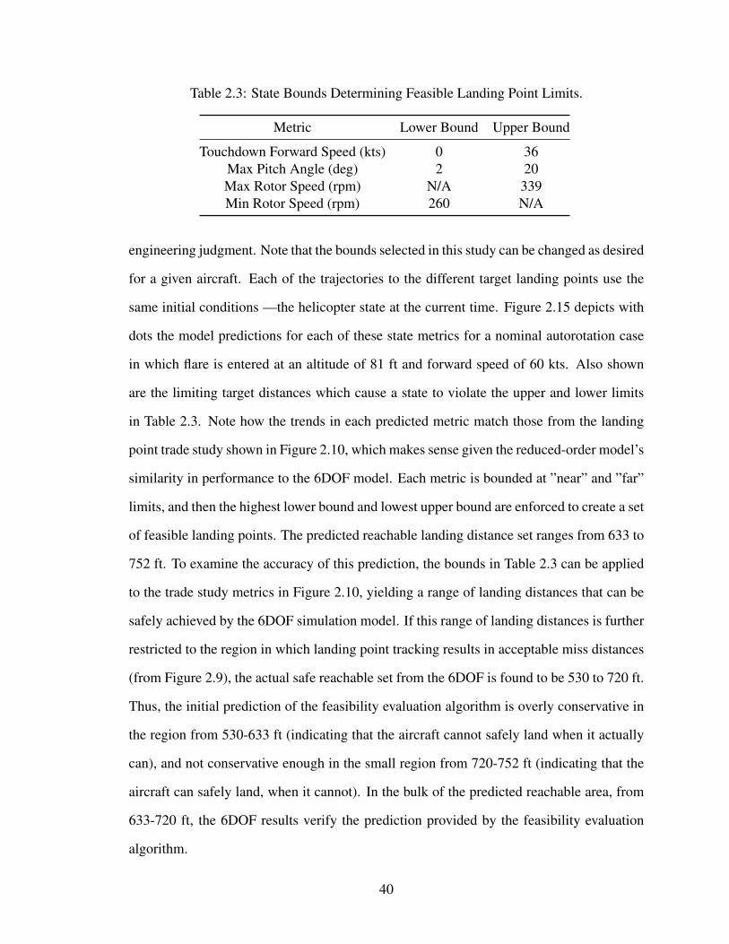
Table 2.3: State Bounds Determining Feasible Landing Point Limits.

Metric Lower Bound Upper Bound

Touchdown Forward Speed (kts) 0 36Max Pitch Angle (deg) 2 20Max Rotor Speed (rpm) N/A 339Min Rotor Speed (rpm) 260 N/A

engineering judgment. Note that the bounds selected in this study can be changed as desired

for a given aircraft. Each of the trajectories to the different target landing points use the

same initial conditions —the helicopter state at the current time. Figure 2.15 depicts with

dots the model predictions for each of these state metrics for a nominal autorotation case

in which flare is entered at an altitude of 81 ft and forward speed of 60 kts. Also shown

are the limiting target distances which cause a state to violate the upper and lower limits

in Table 2.3. Note how the trends in each predicted metric match those from the landing

point trade study shown in Figure 2.10, which makes sense given the reduced-order model’s

similarity in performance to the 6DOF model. Each metric is bounded at ”near” and ”far”

limits, and then the highest lower bound and lowest upper bound are enforced to create a set

of feasible landing points. The predicted reachable landing distance set ranges from 633 to

752 ft. To examine the accuracy of this prediction, the bounds in Table 2.3 can be applied

to the trade study metrics in Figure 2.10, yielding a range of landing distances that can be

safely achieved by the 6DOF simulation model. If this range of landing distances is further

restricted to the region in which landing point tracking results in acceptable miss distances

(from Figure 2.9), the actual safe reachable set from the 6DOF is found to be 530 to 720 ft.

Thus, the initial prediction of the feasibility evaluation algorithm is overly conservative in

the region from 530-633 ft (indicating that the aircraft cannot safely land when it actually

can), and not conservative enough in the small region from 720-752 ft (indicating that the

aircraft can safely land, when it cannot). In the bulk of the predicted reachable area, from

633-720 ft, the 6DOF results verify the prediction provided by the feasibility evaluation

algorithm.

40

400 600 800 1000 1200 1400 1600

0

100

200

400 600 800 1000 1200 1400 1600

-50

0

50

400 600 800 1000 1200 1400 1600

0

50

400 600 800 1000 1200 1400 1600

0

50

Figure 2.15: Feasible Landing Point Evaluation Algorithm Example Case, Initial Solution.

41

400 600 800 1000 1200 1400 1600

0

100

200

400 600 800 1000 1200 1400 1600

-50

0

50

400 600 800 1000 1200 1400 1600

0

50

400 600 800 1000 1200 1400 1600

0

50

Figure 2.16: Feasible Landing Point Evaluation Algorithm Example Case, Updated as Ma-neuver Progresses.

42

As the flare maneuver evolves, the reachable domain can be updated as often as de-

sired using new predictions from the reduced-order model. Figure 2.16 depicts the overall

reachability bounds from initial and updated reachability predictions, recomputed at 2 sec-

ond intervals as the 6DOF simulation evolves (where the 6DOF model is targeting a landing

distance of 670 ft beyond the point of flare entry). As expected, the set of feasible land-

ing points evolves as the maneuver progresses, eventually converging on the target landing

point as the aircraft descends towards touchdown. It is worth mentioning that the average

computation time required to compute each of the 53 feasibility evaluation points (blue

dots) in Figure 2.16 was 8.7 ms using a Python implementation of the point-mass model on

a standard laptop. While the algorithm’s ability to execute in real-time will clearly depend

on the hardware on which it is implemented, this extremely fast execution time provides

some evidence that real-time execution is feasible.

2.3.5 Feasibility Evaluation Algorithm Robustness Studies

Several studies are presented which quantify the robustness of the feasibility evaluation

methodology to variations in the flare entry conditions and winds. Two cases in which au-

torotation is initiated from within the ”avoid region” of the height-velocity diagram for the

AH-1G are considered. Using the landing point tracking scheme coupled to the inner-loop

controller as described above, autorotations from these two different off-nominal conditions

are simulated. Because these cases enter autorotation from a state that should be avoided

during normal operation, they do not reach what could be considered the ”nominal” steady-

state descent condition that is attained during most autorotations initialized outside of the

avoid region. As a result, the inner-loop controller transitions to the flare phase at a differ-

ent speed and/or altitude than the case shown in Figure 2.15. The flare entry states pertinent

to controller performance are summarized in Table 2.4. Note that all the off-nominal cases

enter flare at a higher altitude and vertical speed and lower forward speed than the nominal

case in Figure 2.15. The largest effect on controller performance as a result of the decreased

43

Table 2.4: Nominal and Off-Nominal Flare Entry Conditions.

Flare Entry Flare Entry Flare Entry Target Landing Distance

Case Altitude (ft) Vertical Speed (ft/s) Forward Speed (ft/s) Landing Distance (ft) Error (ft)

Off Nominal 1 118 34 84 504 17Off Nominal 2 127 36 97 700 -8

Headwind 82 23 84 565 -21Tailwind 72 20 109 786 21Nominal 75 21 100 N/A N/A

forward speed at flare entry is a change in the time-to-ground-contact estimate, which is a

strong function of the forward speed. Because the time-to-ground-contact estimate is tuned

for the nominal flare entry case, it is less accurate and both landing point tracking and the

reachability prediction performance are somewhat degraded.

Results from the feasibility evaluation algorithm for these two off-nominal cases are

shown in Figure 2.17 and Figure 2.18. Figure 2.17 depicts the feasible landing point pre-

dictions for the first off-nominal example case, where the reachability bounds are updated

at 2 sec intervals after flare initiation. The initial feasible landing set prediction contains

the ultimate landing site (504 ft downrange of flare entry), and the updated predictions

converge on this point as the vehicle nears touchdown. This indicates that the initial time-

to-ground-contact estimate is accurate, as are subsequent estimates. Also note that the

feasible landing bounds at flare initiation are not that wide (approximately 100 ft) because

the vehicle begins the flare maneuver with a slow forward speed of about 49 kts.

Figure 2.18 shows the feasible landing point predictions for the second off-nominal flare

entry state. In this case, the initial prediction is inaccurate in that it does not contain the

ultimate touchdown point of 700 ft. This is because the time-to-ground-contact estimate

is not accurate initially, i.e., the vehicle is predicted to have less flight time remaining

than it actually does. This inaccuracy is a function of the flare entry conditions shown in

Table 2.4. Note that this case has a similar forward speed to the nominal case, so the initial

kinetic energy as calculated in Equation 2.12 predicts a similar time-to-ground-contact as

44

0 100 200 300 400 500 600 700 800 900

0

100

200

0 100 200 300 400 500 600 700 800 900

-100

0

100

0 100 200 300 400 500 600 700 800 900

0

50

0 100 200 300 400 500 600 700 800 900

0

50

Figure 2.17: Feasible Landing Point Evaluation, First Off-Nominal Flare Entry Condition.

45

0 100 200 300 400 500 600 700 800 900 1000

0

100

200

0 100 200 300 400 500 600 700 800 900 1000

-100

0

100

0 100 200 300 400 500 600 700 800 900 1000

0

50

0 100 200 300 400 500 600 700 800 900 1000

0

50

Figure 2.18: Feasible Landing Point Evaluation, Second Off-Nominal Flare Entry Condi-tion.

46

the nominal case. The flare entry altitude is much higher than the nominal case though, so

the vehicle is able to remain airborne longer than estimated. With subsequent updates the

feasible landing point predictions improve and converge upon the final touchdown point.

Two final examples demonstrating performance of the feasibility evaluation scheme

with steady winds are shown in Figure 2.19 and Figure 2.20. The set of reachable points in

these figures are shifted from the no-wind case shown in Figure 2.16. This shift in reach-

able landing distance is caused by the difference in the vehicle ground speed at flare entry

between the nominal case (Figure 2.16), headwind case (Figure 2.19), and tailwind case

(Figure 2.20). Because a specific airspeed is tracked during steady-state descent to en-

sure optimal glide performance, the ground speed at flare entry varies with the wind speed

and thus the reachable set is farther downrange given a tailwind (because of a faster ini-

tial ground speed) and closer for a headwind (due to a slower initial ground speed). Also,

during the flare maneuver the rotor receives a performance benefit from a headwind and

a performance reduction from a tailwind. This is because when the vehicle pitches up, a

headwind increases inflow through the rotor disk for a given ground speed, while a tailwind

decreases inflow. This results in less rotor speed decay for a headwind during the ultimate

collective increase prior to touchdown. The opposite trend is true for the tailwind case.

The implication of these factors on the feasible landing point set is shown in Figure 2.20,

wherein neither of the final two updates in the tailwind case predict any potential land-

ing sites where the rotor speed does not decay below the acceptable bound. The feasible

landing point predictions shown (in dashed lines) for these updates are reporting only the

bounds in which all other constraints are satisfied, acknowledging that a rotor underspeed

is probable. Despite reporting no reachable points (due to consistent rotor underspeed),

the information produced by the algorithm may still be potentially useful to a pilot or au-

tonomous landing algorithm to identify the landing point which violates the constraints by

the minimal amount.

The results provided throughout this section represent an initial investigation into the

47

0 100 200 300 400 500 600 700 800 900

0

100

200

0 100 200 300 400 500 600 700 800 900

-100

0

100

0 100 200 300 400 500 600 700 800 900

0

50

0 100 200 300 400 500 600 700 800 900

0

50

Figure 2.19: Feasible Landing Point Evaluation, 9kt Headwind Case.

48

100 200 300 400 500 600 700 800 900 1000 1100

0

100

200

100 200 300 400 500 600 700 800 900 1000 1100

0

50

100

0 100 200 300 400 500 600 700 800 900 1000 1100

0

50

0 100 200 300 400 500 600 700 800 900 1000 1100

0

50

Figure 2.20: Feasible Landing Point Evaluation, 6kt Tailwind Case.

49

performance and robustness of the landing point tracking and feasible landing point eval-

uation algorithms. While the algorithms are shown to be reasonably robust to weight and

wind uncertainty, there is certainly room for improvement particularly with respect to time-

to-ground-contact predictions, which are seen to have a noticeable effect on the accuracy of

the feasible landing site prediction scheme in off-nominal conditions. Such enhancements

are beyond the scope of this initial study but are good candidates for future work on this

topic.

2.4 Chapter Summary

This chapter presents the formulation of a landing point tracking approach based in tau the-

ory, which executes very quickly and avoids iterative optimization. A low-order dynamic

model of the helicopter is then utilized to evaluate the kinematically generated trajectories.

An array of trajectories to candidate landing points may be evaluated to yield a sub-optimal

set of reachable landing points in real-time. Numerical results are presented for both of

these methodologies and preliminary robustness studies are also presented. The results

indicate favorable performance of the proposed algorithms, and the reachability determi-

nation scheme could be very helpful for driving a pilot cue during the flare portion of the

maneuver.

However, because these methods are validated in the present section as ancillary ad-

ditions to the control law of [15], they are restricted by the same fundamental limitations

of that control law. Specifically, there is no means for directly enforcing rotor speed con-

straints or even directly controlling rotor speed. This is a necessary function of an au-

tonomous controller that is difficult to effectively achieve when collective and long. cyclic

are decoupled as in this controller. Both collective pitch and vehicle pitch angle affect rotor

speed, therefore a control methodology that considers both simultaneously is necessary to

achieve control over this critical state. Collective and pitch angle also affect the vertical

speed and the forward speed. This describes the underactuated nature of the helicopter in

50

autorotation and provides the motivation for the Model Predictive Controller developed in

the next chapter, which is envisioned as a substitute to the controller from [15].

51

CHAPTER 3

MODEL PREDICTIVE CONTROL

3.1 Chapter Motivation

Controlling rotor speed is not an optional feature of an autonomous autorotation algorithm.

If the rotor speed exceeds its upper bound, structural damage of varying severity may occur

with catastrophic failure of the rotor system as a possible consequence. As the rotor slows

down, the vehicle’s control effectiveness deteriorates. Outside of the continuous rotor speed

bounds, this deterioration may cause total lack of control. Additionally, excessive blade

flapping may occur, which gives no guarantee of clearance between the rotor and the tail

boom. As mentioned in section 2.4, the underactuated nature of the system in autorotation

makes it difficult for a control law to effectively enforce rotor speed constraints and land

the vehicle gently. The nonlinear model predictive controller outlined in this chapter is

developed with the intention of enforcing rotor speed constraints while landing the vehicle

at a safe set of forward and vertical speed conditions.

3.2 Nonlinear Model Predictive Control Law Formulation

This section presents the formulation of a nonlinear model predictive controller (NMPC)

for autorotation using the form presented by Slegers et al. [37] and the helicopter model

derived in [1] and reported in subsection 2.2.1. A key assumption in formulating the con-

trol law is that the autorotation flare is planar – i.e., the aircraft lands straight ahead and

thus only motion in the vertical plane is considered. The NMPC formulation involves

representing the output states and a set of desired trajectories as Taylor series. This in-

cludes analytical expressions for continuous time derivatives for each of the five output

states (downrange distance, forward speed, altitude, vertical speed, and rotor speed). These

52

Taylor series expressions are then used to predict the value of a quadratic cost function

over a given time horizon. Optimal control derivatives are computed at each time step that

minimize the predicted value of this cost function (i.e. tracking error between the outputs

and the desired trajectories). Note that this solution is analytical, thus avoiding iterative

optimization. This is critical in ensuring real-time and deterministic runtime performance

of the controller.

3.2.1 Mathematical Formulation

Defining the state and control vectors as follows,

~x =

x1

x2

x3

x4

x5

=

x

u

z

w

Ω

(3.1)

~u =

u1

u2

=

CTα (3.2)

the dynamic equations from subsection 2.2.1 can be arranged in matrix form as follows

53

x1

x2

x3

x4

x5

=

x2

ρm

(πR4)x25u1 sinu2 − 1

2mρfex2

√x2

2 + x24

x4

g − ρm

(πR4)x25u1 cosu2 − 1

2mρfex4

√x2

2 + x24

− 1ηIRx5

ρ(πR2)(x5R)3Cp

(3.3)

The inflow dynamics are included in the calculation of CP , but the equations are omitted

here for conciseness. Following the development of the nonlinear model predictive control

scheme developed in [37], the outputs must next be represented in the form of Taylor series.

The number of required expansion terms is determined by how many time derivatives of

each state are required before the time derivative of a control term appears. This is one

more derivative than the relative degree of each output Mi + 1. A quadratic, running

cost function is defined to minimize tracking error between the output states and an input

trajectory defined by the designer YD.

J =1

2(YD − Y )TΠ(YD − Y ) (3.4)

where Π is an integration operator integrating state tracking error over a finite time horizon,

given by the expression

Π =

Π1 0 0 0 0

0 Π2 0 0 0

0 0 Π3 0 0

0 0 0 Π4 0

0 0 0 0 Π5

(3.5)

54

Πi = qi

t2−t1(1) 0! 0!

t22−t21(2) 0! 1!

. . .tRi+12 −tRi+1

1

(Ri+1) 0!Ri!

t22−t21(2) 1! 0!

t32−t31(3) 1! 1!

. . .tRi+22 −tRi+2

1

(Ri+2) 1!Ri!

...... . . . ...

tRi+12 −tRi+1

1

(Ri+1)Ri! 0!

tRi+22 −tRi+2

1

(Ri+2)Ri! 1!. . .

t2Ri+12 −t2Ri+1

1

(2Ri+1)Ri!Ri!

(3.6)

where Ri is the order of the Taylor series approximating the ith output. For this derivation,

Ri > Mi. It has been demonstrated in [37] that Ri may be chosen by the designer as a

means of penalizing control action, but the number of terms beyond the relative degree Si

for each output must be the same for every output. That is to say, Si = Ri −Mi must be

equal for all outputs. Πi contains additional tuning parameters: qi, the tracking penalty for

each state and t2, the time horizon. t1 is generally 0 because the optimization starts at the

present time.

After organizing the equations as such, [37] outlines the derivation of the following

control law:

Uc = B−1[KT (Y UD − Y U) + Y L1

D − A] (3.7)

where B is a matrix of output sensitivities to control derivatives and Y UD and Y U represent a

finite number of Taylor series terms used to represent the desired outputs and the predicted

outputs respectively. Y L1D and A are also vectors containing Taylor series terms for the

same. KT is given by

KT =

K1 0 0 0 0

0 K2 0 0 0

0 0 K3 0 0

0 0 0 K4 0

0 0 0 0 K5

(3.8)

where Ki is the first row of (Πi22)−1(Πi

12)T , after Πi is divided into quadrants according to

the terms before and after the relative degree of the output. Note that the dimensions of all

55

the terms in Equation 3.7 remain the same regardless of the chosen Ri. For the dynamical

system used in the work presented here, the key matrices are shown in Appendix A. The

terms shown for the rotor speed state assume the rotor does not enter the Vortex Ring or

Turbulent Wake States as predicted by Momentum Theory. Note that matrix B is rank

deficient and thus has no inverse as required by Equation 3.7. This is a result of the system

being underactuated. For implementation of this controller, the pseudoinverse is used at

this point, which provides the minimum norm solution for the controls.

3.2.2 Reference Trajectory Generation

The control law developed above requires at a minimum a vertical speed and forward speed

reference trajectory as well as a reference rotor speed. Because downrange distance x and

altitude z only serve to provide integral action to vertical speed and forward speed, they

are not necessary for vehicle control and are given 0 tracking cost in this work. There-

fore, no reference trajectories for x and z are presented. Although the presented controller

may certainly be used to perform a steady-state autorotative descent, its primary benefit is

manifested during the flare portion of the maneuver. Because of this, the entry and descent

phases are performed by a PID scheme and the reference trajectories for those portions of

the maneuver are not described here.

The flare forward speed trajectories used in this work are generated according to the

approach developed in section 2.1 and published in [45, 46]. These trajectories are of the

form

ucom(t) = ui

[1− (kopt − 1)uit

xi

]−1− 1kopt−1

(3.9)

where kopt is computed using a time-to-ground-impact estimate at the time of trajectory

generation such that the vehicle arrives at the desired landing point at the time of touch-

down. This trajectory is based on tau theory and has been shown to produce favorable

results when tracked to a landing during autorotation (section 2.3).

Flare entry is determined according to the following equation, which assumes an ex-

56

ponential decay from the present vertical speed to some arbitrary, small vertical speed at

touchdown d. It also assumes a decay time constant of τ and a time-to-impact of T . The

flare entry height is given by,

hi =(wi − d)T

τ(1− e−τ ) + dt (3.10)

After flare is initiated, Equation 3.11 is tracked as the vertical speed reference trajectory.

wcom(t) = (wi − d)e−τt/T + d (3.11)

To increase the robustness of the landings by accounting for tracking error as the flare

progresses, the vertical speed trajectory is periodically updated as the flare progresses. This

is accomplished by solving Equation 3.12 for new values of τ that result in a slow vertical

speed at the time of touchdown. The time-to-ground-impact estimate used for each update

during flare is determined by a kinetic energy scale factor as in section 2.1. Although it is

not necessary to include such updates, doing so increases reliability of successful landings.

Because these updates are unnecessary, if a solution does not exist to Equation 3.12, the

update is simply skipped and the previous trajectory remains as the commanded one.

h(T ) = 0 = −(wi − d)T

τ(1− e−τt/T ) + dt+ hi (3.12)

3.2.3 State-Dependent Rotor Speed Penalty

The reference rotor speed is the nominal autorotation rotor speed for the vehicle. Given a

constant rotor speed tracking gain, it is the objective of the controller to mitigate deviation

from this value as the landing trajectory is tracked. However, some variation in rotor speed

may be acceptable (within bounds) to enable better tracking of the forward or vertical speed

trajectories. The formulation of the present control scheme enables the use of a nonlinear,

state-dependent rotor speed tracking penalty. Figure 3.1 depicts the variable gain used in

57

the present work. Note the dead zone when the rotor speed is close to nominal that allows

the rotor speed to vary freely when in this region. As the rotor speed varies more from the

nominal, the penalty increases exponentially until the rotor speed reaches a boundary. The

boundaries are shaped by the control designer based on the desired response and particular

vehicle characteristics. Here, the maximum bound used is the absolute maximum for the

AH-1G vehicle (104%) and the minimum bound is the continuous minimum bound (91%)

as given by [44].

90 95 100 105

% Rotor Speed

0

0.5

1

1.5

2

2.5

Ro

tor

Sp

ee

d T

rackin

g P

en

alty G

ain

Below 100%

Deadzone

Above 100%

Figure 3.1: State-Dependent Rotor Speed Tracking Penalty.

3.2.4 Control Implementation

Figure 3.2 is a block diagram depicting the implementation of the MPC scheme with the

helicopter simulation model. One interesting feature of this figure involves the conversion

of the controller outputs to actual collective and longitudinal cyclic controls. The controller

outputs optimal time derivatives of the thrust coefficient (CT ) and tip path plane angle (α).

These must be integrated at each control update to yield the present commanded control

positions. Note that the model derived in [1] assumes that the vehicle pitch angle θ is equal

to the opposite of the tip path plane angle. There is no direct mapping between desired pitch

angle and longitudinal cyclic position, so this commanded pitch angle must be tracked by

an inner loop PID controller. There is such a relationship for coefficient of thrust and

58

collective position, which is shown in Equation 3.13 and derived in [1]. The NMPC acts as

both an outer loop controller (for pitch angle) and an inner loop controller (for thrust, via

an algebraic mapping to the collective).

Figure 3.2: MPC Implementation with Helicopter Simulator.

θ75 =(1 + 3

2µ2)(6Ct

aσ) + 3

2λ(1− 1

2µ2)

1− µ2 + 94µ4

(3.13)

3.3 Results

3.3.1 Simulation Model

The simulation model used for this work is described here, with a more extensive descrip-

tion available in [15]. The ARMCOP model [41, 47, 48] is the basis for the model used

here, although several additions are made for increased accuracy including dynamic inflow,

blade stall, and ground effect. This model includes 22 states: 12 rigid body states for the

vehicle, 1 rotor speed state, 6 main rotor flapping states and 3 dynamic inflow states. These

states are propagated forward using a fourth order Runge-Kutta integrator with a timestep

59

of 0.001s. Linear aerodynamic effects are considered from the fuselage and empennage

and horizontal and vertical stabilizers, and a simplified fuselage drag model is used to cal-

culate downwash components. The tail rotor forces and moments are calculated assuming

uniform inflow, and a scale factor is applied to the main rotor speed during autorotation to

determine the tail rotor speed.

The main rotor forces and moments are calculated numerically using a blade element

approach. The rotor disk is divided into 30 azimuthal stations and is broken into 15 radial

elements at each station. Look up tables from [49] are referenced to account for blade

elements that may be stalled, although dynamic stall is neglected. After the forces and

moments are calculated on each element, they are summed, averaged and normalized. The

net torque required is determined from these calculations, and during autorotation, this

torque determines the rotor acceleration Ω. A second order model of the blade flapping

dynamics is propagated to determine the first harmonic flapping components β0, β1s, β1c

(although the coning angle β0 is always 0 for the teetering rotor used here).

The dynamic inflow model of [42, 43] is used to increase accuracy during the rapidly

changing inflow seen in autorotative flare. This is a 3 state model which describes the

induced inflow at any point on the rotor disk according to the following equation

λi(r, ψ) = λ0 + λsr

Rsinψ + λc

r

Rcosψ (3.14)

where the states λ0, λs, and λc are propagated forward according to the following equation

[M ]

λ0

λs

λc

+ [L]−1

λ0

λs

λc

= ~C (3.15)

where [M ] is a matrix of apparent mass terms, [L] takes into account sideslip angle and

60

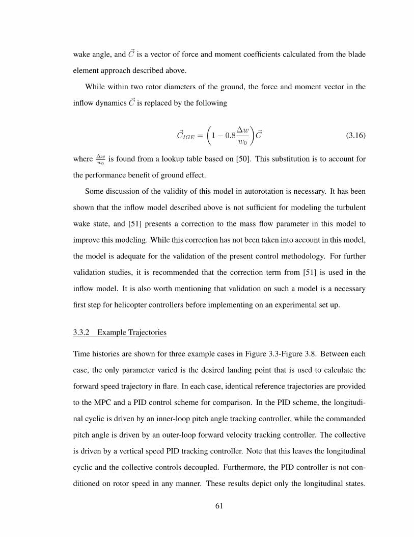
wake angle, and ~C is a vector of force and moment coefficients calculated from the blade

element approach described above.

While within two rotor diameters of the ground, the force and moment vector in the

inflow dynamics ~C is replaced by the following

~CIGE =

(1− 0.8

∆w

w0

)~C (3.16)

where ∆ww0

is found from a lookup table based on [50]. This substitution is to account for

the performance benefit of ground effect.

Some discussion of the validity of this model in autorotation is necessary. It has been

shown that the inflow model described above is not sufficient for modeling the turbulent

wake state, and [51] presents a correction to the mass flow parameter in this model to

improve this modeling. While this correction has not been taken into account in this model,

the model is adequate for the validation of the present control methodology. For further

validation studies, it is recommended that the correction term from [51] is used in the

inflow model. It is also worth mentioning that validation on such a model is a necessary

first step for helicopter controllers before implementing on an experimental set up.

3.3.2 Example Trajectories

Time histories are shown for three example cases in Figure 3.3-Figure 3.8. Between each

case, the only parameter varied is the desired landing point that is used to calculate the

forward speed trajectory in flare. In each case, identical reference trajectories are provided

to the MPC and a PID control scheme for comparison. In the PID scheme, the longitudi-

nal cyclic is driven by an inner-loop pitch angle tracking controller, while the commanded

pitch angle is driven by an outer-loop forward velocity tracking controller. The collective

is driven by a vertical speed PID tracking controller. Note that this leaves the longitudinal

cyclic and the collective controls decoupled. Furthermore, the PID controller is not con-

ditioned on rotor speed in any manner. These results depict only the longitudinal states.

61

In these cases, the pedal controls are driven by a PID regulating sideslip angle to 0, and a

lateral cyclic cascaded PID control tracks a constant heading setpoint. It is assumed that

any necessary lateral positioning of the aircraft is accomplished prior to flare entry.

By comparing the formulation of the MPC with a PID controller the benefits of such

an approach can be hypothesized. Because the MPC uses a dynamic model to predict

the response of the helicopter to a set of control inputs, it is able to forecast whether a

state will violate a constraint and can adjust the controls accordingly to prevent the bound

from being broken. Additionally, this MPC approach is Multi-Input Multi-Output, which

allows it to take into account the coupling between control channels. A PID controller

functions by looking only at the error in the feedback and is typically Single-Input Single-

Output (SISO). Because a PID controller considers the error signal, it is difficult for it to

predict a bound will be broken before it actually occurs. Because PID controllers are SISO,

underactuated systems (such as a helicopter in autorotation) may have output states that are

left unregulated. For example, in the results shown here, the PID controller controls only

vertical speed and forward speed, which leaves rotor speed to float freely, possibly violating

its safe operating bounds.

In Example Case 1 (Figure 3.3 and Figure 3.4) the forward speed profile is targeting a

landing point that is 550 ft passed the point of flare entry. This is a relatively close-in target

point, meaning the reference forward speed will command a more rapid deceleration. This

is achieved by pitching the vehicle up more aggressively, which leads to increased rotor

inflow and an accompanying increase in rotor speed. In Figure 3.3 the PID controller

tracks forward speed well but exceeds the absolute maximum rotor speed bound, while the

MPC sacrifices forward speed tracking to prevent the rotor speed from breaking that hard

constraint. Figure 3.4 shows that this is done by commanding a less aggressive pitch up,

and a slight pitch down while the rotor speed is near the maximum bound.

Figure 3.5 and Figure 3.6 (Example Case 2) show a trajectory targeting a landing point

that is 1010 ft downrange—a relatively far target point at this flare altitude. Here, the trajec-

62

tory commands a much more gradual deceleration to prolong the glide distance. However,

as Figure 3.5 shows in the PID case, if the glide is stretched too far the rotor speed begins

to decay. This is the result of a commanded pitch up that is too gradual, resulting in insuffi-

cient inflow to the rotor to safely track the commanded vertical speed. The MPC allows the

rotor speed to decay to extend the glide as much as safely possible, but when the rotor speed

approaches the minimum continuous bound, the MPC commands a pitch up that maintains

the rotor speed within its continuous bound. The MPC also lowers collective compared

with the PID scheme in order to keep the rotor speed from decaying as rapidly. This results

in a higher rotor speed at touchdown. For comparison, at the time that the open-loop pitch

over is commanded, the rotor speed is 5.2% higher for the MPC than the PID. It is also

worth noting that the MPC trajectory spends less time outside the continuous bound, which

may be an unsafe area of operation depending on the platform. For comparison, the MPC

spends 2.75 seconds less outside this bound than the PID. This is a reduction of 56%.

These trajectories show the benefit of the MPC scheme over the simpler PID control

scheme. When given a rapidly-generated, suboptimal trajectory, the MPC is able to sacri-

fice forward velocity and landing point tracking to meet rotor speed constraints. By treating

target landing distance as a soft constraint, it allows the controller to enforce the rotor speed

bounds as hard constraints. Enabling the controller designer to control this trade off is a

novel feature for an autorotation controller, which is a step towards online implementation

by potentially removing the need for optimizing the reference trajectory in real-time with

regard for dynamic constraints. On the topic of runtime, it is necessary to mention that

average execution time of this MPC scheme is 1.1ms. This implementation is written in

python and executed by a 2.6GHz quad-core Intel Core i7 processor on a standard lap-

top. This rapid execution time (which omits delays from sensor feedback) indicates that

real-time execution on-board an embedded controller is likely possible; however, execution

time must be characterized on the actual hardware to be certain of real-time performance.

The model parameters used here are listed in Table 3.1 and are identical to the low-order

63

model parameters shown in Table 2.2, except for cd0, which is used as a tuning parameter

for rotor speed performance. While not necessary for a single landing trajectory, vertical

speed trajectory updates are included at 3 second intervals to mitigate the effects of track-

ing error. Including these updates improves landing reliability across varied target landing

points. Also, it is important to note that when the vehicle is within 3.5 ft of the ground, the

output from the MPC is overridden by a pitch angle commanded to 0. This has the effect of

bringing the pitch angle to a safe level for touchdown. Additionally, for the MPC cases, the

forward speed error is saturated outside of the bounds [-4, +5] ft/s. Without this saturation,

if the MPC sacrifices forward speed tracking to regulate rotor speed, the compounding error

in forward speed starts to dominate the penalty terms from the rotor speed. By saturating

the forward speed error, the MPC is able to most effectively control rotor speed. Equa-

tion 3.13 is perhaps an overly simplistic relationship between the coefficient of thrust and

the collective position because it assumes uniform inflow. To utilize the expression in this

application, a is used as a tuning parameter to match the commanded CT from the MPC

scheme with the resulting CT from the medium-fidelity model. The tuning done in steady

state yields a good match for the initial portion of the flare, but at low vertical speeds, a

mismatch in this expression results in poor vertical speed tracking. To account for this, a

is increased by an offset of 0.46 when z < 1.5ft/s. This results in a better match between

the low and medium fidelity models, and improved tracking performance.

Example Case 3 shows a trajectory targeting a landing point 775 ft downrange of flare

entry and is depicted in Figure 3.7 and Figure 3.8. This case demonstrates a more nominal

landing distance rather than the extremes shown in the prior two examples. When not

forced into a tradeoff between rotor speed constraints and trajectory tracking, the MPC

performs comparably to the PID control scheme (as would be expected). The commanded

pitch angles produced by the MPC are more aggressive than the PID case. This can be

controlled through two tuning parameters—the number of Taylor series terms included in

the optimization problem (Ri) and the prediction horizon of the MPC (t2).

64

3.3.3 Trade Studies

To demonstrate the effect of these tuning parameters, two trade studies are presented wherein

the number of Taylor series terms and the time horizon are varied. Figure 3.9 and Fig-

ure 3.10 show the effects of including more or fewer terms in the optimization problem

with the time horizon being held constant at t2 = 2.25s. It is worth noting that solving for

additional analytical derivatives of the output terms is not necessary to increase the number

of Taylor series terms in this control law. This is because the contents of Ki change with

the number of terms, but its dimensions remain the same. Figure 3.9 shows that with an

increased number of terms, the trajectory tracking is more accurate. However, Figure 3.10

shows that more aggressive control inputs accompany the better tracking. The time horizon

is another available tuning parameter. As expected with many MPC schemes, the shorter

the time horizon, the greedier the controller control action. To illustrate this trade along

with the effects of number of Taylor series terms, Figure 3.11 and Figure 3.12 show three

cases with varied time horizon and number of Taylor series terms, but all with comparable

tracking performance. Because performance can be tuned to be similar across these two

tuning parameters, the desired time horizon can be selected according to the desired maneu-

ver performance and the accurate prediction horizon of the low-order model. For the results

presented outside of these two studies, 8 Taylor series terms are used (Ri = 8, Si = 6) and

the time horizon is chosen to be 3.3s. With a time horizon much longer than this, the ac-

curacy of the low-order model begins to deteriorate. Due to the highly nonlinear nature of

a helicopter in autorotative flare, this 3.3s time horizon is significantly longer than could

be attained with many linear dynamic models. This points to the benefit of using nonlinear

MPC as opposed to a more standard linear MPC approach.

Figure 3.13 and Figure 3.14 show the results of a trade study comparing performance

of the MPC to the PID across a range of target landing distances from the flare entry point.

The MPC performs comparably to the PID scheme in terms of landing distance error, but

outperforms it on all other metrics. The vertical speed at touchdown is lower for all cases.

65

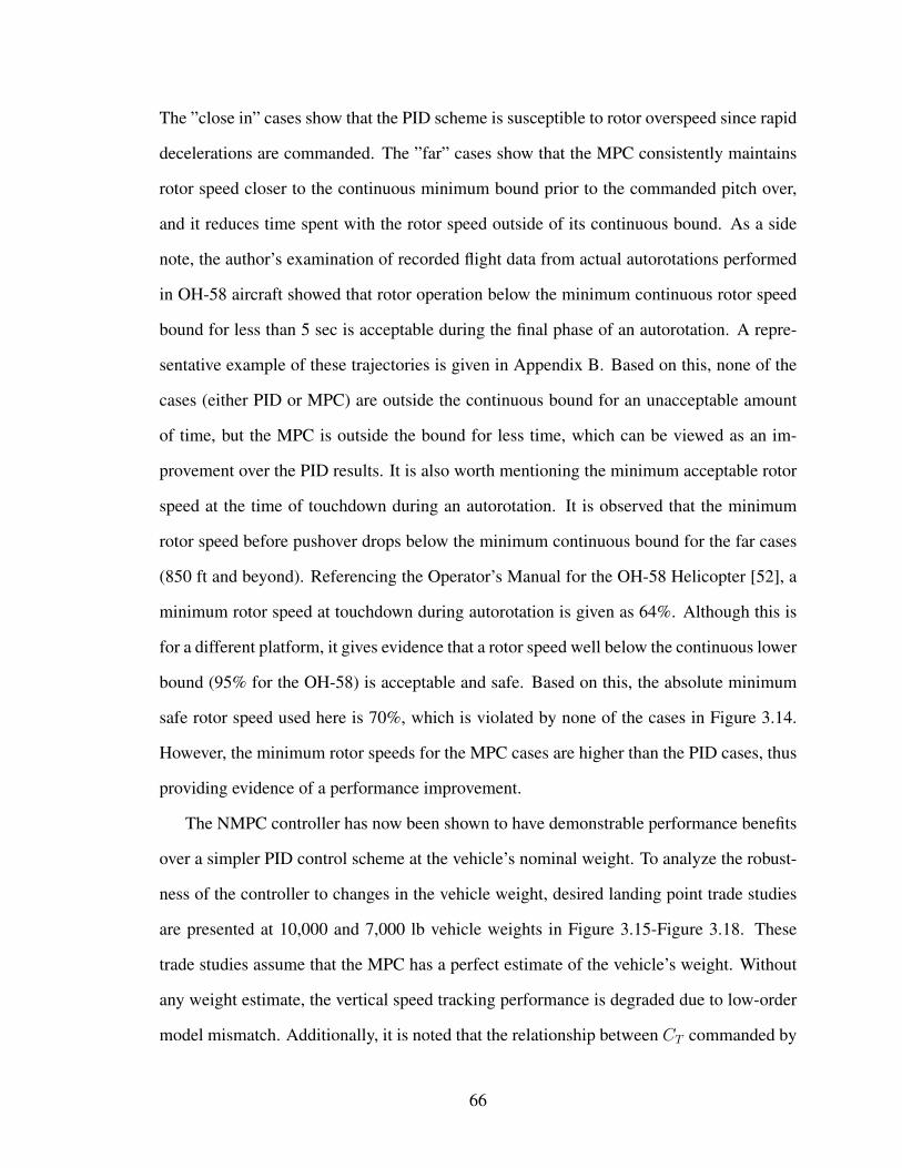
The ”close in” cases show that the PID scheme is susceptible to rotor overspeed since rapid

decelerations are commanded. The ”far” cases show that the MPC consistently maintains

rotor speed closer to the continuous minimum bound prior to the commanded pitch over,

and it reduces time spent with the rotor speed outside of its continuous bound. As a side

note, the author’s examination of recorded flight data from actual autorotations performed

in OH-58 aircraft showed that rotor operation below the minimum continuous rotor speed

bound for less than 5 sec is acceptable during the final phase of an autorotation. A repre-

sentative example of these trajectories is given in Appendix B. Based on this, none of the

cases (either PID or MPC) are outside the continuous bound for an unacceptable amount

of time, but the MPC is outside the bound for less time, which can be viewed as an im-

provement over the PID results. It is also worth mentioning the minimum acceptable rotor

speed at the time of touchdown during an autorotation. It is observed that the minimum

rotor speed before pushover drops below the minimum continuous bound for the far cases

(850 ft and beyond). Referencing the Operator’s Manual for the OH-58 Helicopter [52], a

minimum rotor speed at touchdown during autorotation is given as 64%. Although this is

for a different platform, it gives evidence that a rotor speed well below the continuous lower

bound (95% for the OH-58) is acceptable and safe. Based on this, the absolute minimum

safe rotor speed used here is 70%, which is violated by none of the cases in Figure 3.14.

However, the minimum rotor speeds for the MPC cases are higher than the PID cases, thus

providing evidence of a performance improvement.

The NMPC controller has now been shown to have demonstrable performance benefits

over a simpler PID control scheme at the vehicle’s nominal weight. To analyze the robust-

ness of the controller to changes in the vehicle weight, desired landing point trade studies

are presented at 10,000 and 7,000 lb vehicle weights in Figure 3.15-Figure 3.18. These

trade studies assume that the MPC has a perfect estimate of the vehicle’s weight. Without

any weight estimate, the vertical speed tracking performance is degraded due to low-order

model mismatch. Additionally, it is noted that the relationship between CT commanded by

66

the MPC and that calculated from the 6DOF model do not match when the mass is varied.

To correct for this mismatch, the lift curve slope in Equation 3.13 is used as a tuning pa-

rameter. These changes are recorded in Table 3.1. Figure 3.15 and Figure 3.16 show that

landing point tracking is the metric most affected by the increase in vehicle gross weight.

This is a result of the same vertical speed trajectory being commanded regardless of the

change in weight. This landing distance error could likely be improved given different tra-

jectories for each gross weight; however, the purpose of this study is to highlight the benefit

of the controller over a PID controller at various vehicle weights, which is shown in these

results. Even at the maximum vehicle weight (a condition particularly susceptible to rotor

overspeed), the controller is able to prevent rotor overspeed in cases where the PID con-

troller does overspeed the rotor. Also, the minimum rotor speed performance is even more

improved over the PID case than at the nominal gross weight. Figure 3.17 and Figure 3.18

show that the controller is also robust to a decrease in gross weight and that it is able to

yield its key performance benefits in light vehicle configurations as well. This is indicated

by improved rotor speed performance over the PID at this weight while still performing

comparably on landing point tracking.

3.3.4 Monte Carlo Analyses

Monte Carlo studies were conducted to investigate the robustness of the present control

scheme. A Monte Carlo study is presented, where 500 cases are run with varied target

landing distance and vehicle weight. The target landing distance and the weight are varied

between 550 to 1,010ft and 7,000 to 10,000lbs respectively using uniform distributions.

Because it is difficult to achieve perfectly accurate, real-time estimates of the helicopter

mass, the sensitivity of the MPC to mass estimate must be examined. To accomplish this,

Gaussian error is included in the controller’s mass parameter. The standard deviation of

this error is 3.3% of the vehicle’s weight. For each case a is determined using the MPC

mass estimate and a quadratic regression of the a values shown in Table 3.1. To determine

67

Table 3.1: Reduced Order Model, Trajectory, and Controller Parameters

Reduced Order Model Parameters

Vehicle Mass, m[slugs] 258 (8300lbs)Rotor Efficiency Factor, η 0.97

Induced Power Factor, Kind 1.05Air Density, ρ [slugs/ft3] 0.002378Main Rotor Radius, R [ft] 22

Rotor Moment of Inertia, IR [slugs− ft2] 2770Mean Profile Drag Coefficient, cd0 0.0048

Equivalent Flat Plate Drag Area, fe [ft2] 10.0Rotor Solidity Ratio, σ 0.0651

Trajectory Parameters

d [ft/s] 1.5τ [s] 3.5Ti [s] 12.2

Controller Parameters

a (8,300lbs) 2.14a (10,00lbs) 2.52a (7,000lbs) 1.95

q2 0.15q4 10

68

whether a case is successful, the success criteria collected in Table 3.2 are applied to the

state time histories. With the exception of the continuous rotor speed requirements, the

states at the time of vehicle impact are used to assess the quality of landing. These suc-

cess criteria are identical to those in Table 2.1 with the addition of the ”time outside of

continuous rotor speed bounds” metric which was determined with reference to data taken

from actual piloted autorotations (Appendix B). Figure 3.19 shows the success of the cases

plotted with the target landing distance vs vehicle weight. Of the 500 cases, 351 (70%)

are successful, 136 (27%) are marginal, and 13 (3%) are crash landings. It is noted that

many of the marginal cases fall between 800 and 950ft. target landing distance, across the

entire range of weights. Figure 3.20 shows the weight estimate error vs the target landing

distance. There is a grouping of marginal cases between the same target landing distances,

and this appears to be independent of the vehicle mass estimate. All but 2 of the marginal

cases violate the pitch angle and/or pitch rate success criteria only. This indicates that for

the target landing distance range between 800 and 950ft, the open-loop pitch down at the

end of the maneuver is either too aggressive or mistimed. This could be improved with tun-

ing changes; however, the goal of the study is to demonstrate MPC tracking robustness to

weight variation and weight estimate error, which is accomplished despite these marginal

cases. There is a group of failed cases in the light weight and close in landing points.

These cases are briefly exceeding the maximum rotor speed boundary. Note in Figure 3.20

that they all have considerable underestimates of the vehicle weight, and this is causing the

MPC to overspeed the rotor. The designer could increase the rotor speed penalty to account

for this condition.

A final Monte Carlo study is presented to demonstrate the robustness of the controller to

maneuver entry condition. Figure 3.21 shows the results of this study as a Height-Velocity

(HV) Diagram with the avoid region for the AH-1G taken from [53]. The success criteria

from Table 3.2 are also applied in this study. The control scheme performance outside the

avoid region with the presented parameters is almost uniformly successful. This indicates

69

Table 3.2: Criteria Used to Determine the Success of an Autorotative Landing (Restated).

Vehicle State Condition for Condition forat Touchdown Successful Landing Marginal Landing

Forward Speed, x <36kt <42ktLateral Speed, y <3ft/s <6ft/sVertical Speed, z <10ft/s <15ft/s

Absolute Rotor Speed Bounds, Ω 70%< Ω < 104% 70%< Ω < 104%Time Outside Continuous Rotor Speed Bounds 5 s 10 s

Roll Angle, φ <5 <10

Pitch Angle, θ -5 < θ <10 -10 < θ <15

Roll Rate, p <8/s <15/sPitch Rate, q <10/s <20/sYaw Rate, r <8/s <15/s

*These bounds are applied to the absolute value of each metric unless noted otherwise.Simulations that do not meet these criteria are considered failed landings.

that the control scheme is capable of achieving successful landings throughout most of

the vehicle’s flight envelope. Much of the adjustment is accomplished by the PID control

scheme in the steady descent portion of the maneuver, which is tracking 60kts forward

speed and 98% rotor speed, so many of the cases arrive at a common flare entry state, from

which the MPC scheme tracks the nominal trajectory to a successful touchdown. The few

marginal or failed cases outside the avoid region are likely brought to unsafe conditions

by this PID scheme prior to MPC takeover. These cases could perhaps be improved by

tracking a different set of forward speed conditions during steady descent or may require a

dedicated control scheme for the low altitude entry conditions. Satisfactory robustness to

initial energy condition is achieved by the controller in this study.

Overall, the NMPC controller formulated here is shown to have significant advantages

over simpler, model-free schemes. The main benefit of the NMPC algorithm is its use of

a model in predicting how immediate actions will lead to future changes in the dynam-

ics. These predictions can then be used to intelligently trade off competing constraints and

objectives. Such an ability is highly useful in real-world autorotations given the numer-

ous vehicle and environmental constraints that affect the overall outcome of the maneuver.

70

Suggestions for future work are given in subsection 5.2.2.

71

30 32 34 36 38 40 42

Time (s)

0

10

20

30

40

50

60

Fo

rwa

rd S

pe

ed

(kts

)

PID Actual

PID Commanded

MPC Actual

MPC Commanded

Max Touchdown Bound

30 32 34 36 38 40 42

Time (s)

0

5

10

15

20

25

Ve

rtic

al S

pe

ed

(ft

/s)

PID Actual

PID Commanded

MPC Actual

MPC Commanded

Max Touchdown Bound

30 32 34 36 38 40 42

Time (s)

85

90

95

100

105

110

Ro

tor

Sp

ee

d (

%)

PID Actual

MPC Actual

Absolute Maximum Bound

Continuous Minimum Bound

Figure 3.3: Example Case 1 Output States: Targeting 550 ft downrange.

72

30 32 34 36 38 40 42

Time (s)

-5

0

5

10

15

20

Pitch

An

gle

(d

eg

.)

Commanded PID

Actual PID

Commanded MPC

Actual MPC

30 32 34 36 38 40 42

Time (s)

7

8

9

10

11

12

13

14

15

Ma

in R

oto

r C

olle

ctive

, 0

MR

(d

eg

.)

PID

MPC

30 32 34 36 38 40 42

Time (s)

-15

-10

-5

0

5

10

Lo

ng

itu

din

al C

yclic

, 1

s (

de

g.)

PID

MPC

Figure 3.4: Example Case 1 Controls: Targeting 550 ft downrange.

73

30 32 34 36 38 40 42

Time (s)

25

30

35

40

45

50

55

60

Fo

rwa

rd S

pe

ed

(kts

)

PID Actual

PID Commanded

MPC Actual

MPC Commanded

Max Touchdown Bound

30 32 34 36 38 40 42

Time (s)

0

5

10

15

20

25

Ve

rtic

al S

pe

ed

(ft

/s)

PID Actual

PID Commanded

MPC Actual

MPC Commanded

Max Touchdown Bound

30 32 34 36 38 40 42

Time (s)

80

85

90

95

100

105

Ro

tor

Sp

ee

d (

%)

PID Actual

MPC Actual

Absolute Maximum Bound

Continuous Minimum Bound

Figure 3.5: Example Case 2 Output States: Targeting 1,010 ft downrange.

74

30 32 34 36 38 40 42

Time (s)

-5

0

5

10

15

Pitch

An

gle

(d

eg

.)

Commanded PID

Actual PID

Commanded MPC

Actual MPC

30 32 34 36 38 40 42

Time (s)

7

8

9

10

11

12

13

14

15

Ma

in R

oto

r C

olle

ctive

, 0

MR

(d

eg

.)

PID

MPC

30 32 34 36 38 40 42

Time (s)

-15

-10

-5

0

5

10

Lo

ng

itu

din

al C

yclic

, 1

s (

de

g.)

PID

MPC

Figure 3.6: Example Case 2 Controls: Targeting 1,010 ft downrange.

75

30 32 34 36 38 40 42

Time (s)

25

30

35

40

45

50

55

60

Fo

rwa

rd S

pe

ed

(kts

)

PID Actual

PID Commanded

MPC Actual

MPC Commanded

Max Touchdown Bound

30 32 34 36 38 40 42

Time (s)

0

5

10

15

20

25

Ve

rtic

al S

pe

ed

(ft

/s)

PID Actual

PID Commanded

MPC Actual

MPC Commanded

Max Touchdown Bound

30 32 34 36 38 40 42

Time (s)

90

95

100

105

Ro

tor

Sp

ee

d (

%)

PID Actual

MPC Actual

Absolute Maximum Bound

Continuous Minimum Bound

Figure 3.7: Example Case 3 Output States: Targeting 775 ft downrange.

76

30 32 34 36 38 40 42

Time (s)

-5

0

5

10

15

Pitch

An

gle

(d

eg

.)

Commanded PID

Actual PID

Commanded MPC

Actual MPC

30 32 34 36 38 40 42

Time (s)

7

8

9

10

11

12

13

14

15

Ma

in R

oto

r C

olle

ctive

, 0

MR

(d

eg

.)

PID

MPC

30 32 34 36 38 40 42

Time (s)

-15

-10

-5

0

5

10

Lo

ng

itu

din

al C

yclic

, 1

s (

de

g.)

PID

MPC

Figure 3.8: Example Case 3 Controls: Targeting 775 ft downrange.

77

30 32 34 36 38 40 42 44

Time (s)

0

10

20

30

40

50

60

Fo

rwa

rd S

pe

ed

(kts

)

S = 2

S = 3

S = 4

30 32 34 36 38 40 42 44

Time (s)

0

5

10

15

20

25

Ve

rtic

al S

pe

ed

(ft

/s)

S = 2

S = 3

S = 4

30 32 34 36 38 40 42 44

Time (s)

75

80

85

90

95

100

105

Ro

tor

Sp

ee

d (

%)

S = 2

S = 3

S = 4

Commanded

Figure 3.9: Comparison of Number of Taylor Series Terms with Constant Time Horizon.

78

30 32 34 36 38 40 42 44

Time (s)

-5

0

5

10

15

20

Pitch

An

gle

(d

eg

.)

S = 2 Com.

S = 2

S = 3 Com.

S = 3

S = 4 Com.

S = 4

30 32 34 36 38 40 42 44

Time (s)

6

8

10

12

14

16

18

20

Ma

in R

oto

r C

olle

ctive

0M

R

(d

eg

.)

S = 2

S = 3

S = 4

30 32 34 36 38 40 42 44

Time (s)

-5

0

5

10

15

Lo

ng

. C

yclic

, 1

s (

de

g.) S = 2

S = 3

S = 4

Figure 3.10: Comparison of Number of Taylor Series Terms with Constant Time HorizonCont.

79

30 31 32 33 34 35 36 37 38 39 40

Time (s)

20

30

40

50

60

Fo

rwa

rd S

pe

ed

(kts

)

S = 1, t2 = 0.5

S = 4, t2 = 2.5

S = 6, t2 = 3.3

30 31 32 33 34 35 36 37 38 39 40

Time (s)

0

5

10

15

20

25

Ve

rtic

al S

pe

ed

(ft

/s) S = 1, t

2 = 0.5

S = 4, t2 = 2.5

S = 6, t2 = 3.3

30 31 32 33 34 35 36 37 38 39 40

Time (s)

90

95

100

105

Ro

tor

Sp

ee

d (

%)

S = 1, t2 = 0.5

S = 4, t2 = 2.5

S = 6, t2 = 3.3

Commanded

Figure 3.11: Comparison of Number of Taylor Series Terms with Varied Time Horizon.

80

30 31 32 33 34 35 36 37 38 39 40

Time (s)

-5

0

5

10

15

20

Pitch

An

gle

(d

eg

.)

S = 1, t2 = 0.5 Com.

S = 1, t2 = 0.5

S = 4, t2 = 2.5 Com.

S = 4, t2 = 2.5

S = 6, t2 = 3.3 Com.

S = 6, t2 = 3.3

30 31 32 33 34 35 36 37 38 39 40

Time (s)

7

8

9

10

11

12

13

14

15

Ma

in R

oto

r C

olle

ctive

0M

R

(d

eg

.)

S = 1, t2 = 0.5

S = 4, t2 = 2.5

S = 6, t2 = 3.3

30 31 32 33 34 35 36 37 38 39 40

Time (s)

-5

0

5

10

15

Lo

ng

. C

yclic

, 1

s (

de

g.) S = 1, t

2 = 0.5

S = 4, t2 = 2.5

S = 6, t2 = 3.3

Figure 3.12: Comparison of Number of Taylor Series Terms with Varied Time HorizonCont.

81

550 600 650 700 750 800 850 900 950 1000 1050

-50

0

50

100

150

La

nd

ing

Dis

tan

ce

Err

or

(ft.

)

PID

MPC

550 600 650 700 750 800 850 900 950 1000 105010

15

20

25

30

35

40

45

Fo

rwa

rd S

pe

ed

at

To

uch

do

wn

(kts

)

PID

MPC

Successful Touchdown

550 600 650 700 750 800 850 900 950 1000 1050

Target Landing Distance (ft.)

1

2

3

4

5

6

7

8

Ve

rtic

al S

pe

ed

at

To

uch

do

wn

(ft

/s)

PID

MPC

Successful Touchdown

Figure 3.13: Landing Point Tracking Trade Study PID Comparison Metrics, Gross Weight8,300lbs.

82

550 600 650 700 750 800 850 900 950 1000 105096

98

100

102

104

106

Ma

x R

oto

r S

pe

ed

(%

)

PID

MPC

Absolute Maximum Bound

550 600 650 700 750 800 850 900 950 1000 105080

85

90

95

100

105

Ro

tor

Sp

ee

d a

t P

ush

ove

r (%

)

PID

MPC

Minimum Continuous Bound

550 600 650 700 750 800 850 900 950 1000 1050

Target Landing Distance (ft.)

0

1

2

3

4

5

Tim

e B

elo

w R

oto

r S

pe

ed

Bo

un

d (

s)

PID

MPC

Figure 3.14: Landing Point Tracking Trade Study PID Comparison Metrics, Gross Weight8,300lbs Cont.

83

550 600 650 700 750 800 850 900 950 1000 1050-100

-50

0

50

100

150

200

250

La

nd

ing

Dis

tan

ce

Err

or

(ft.

)

PID

MPC

550 600 650 700 750 800 850 900 950 1000 105010

15

20

25

30

35

40

45

Fo

rwa

rd S

pe

ed

at

To

uch

do

wn

(kts

)

PID

MPC

Successful Touchdown

550 600 650 700 750 800 850 900 950 1000 1050

Target Landing Distance (ft.)

1

2

3

4

5

6

7

8

Ve

rtic

al S

pe

ed

at

To

uch

do

wn

(ft

/s)

PID

MPC

Successful Touchdown

Figure 3.15: Landing Point Tracking Trade Study PID Comparison Metrics, Gross Weight10,000lbs.

84

550 600 650 700 750 800 850 900 950 1000 105096

98

100

102

104

106

108

Ma

x R

oto

r S

pe

ed

(%

)

PID

MPC

Absolute Maximum Bound

550 600 650 700 750 800 850 900 950 1000 105075

80

85

90

95

100

Ro

tor

Sp

ee

d a

t P

ush

ove

r (%

)

PID

MPC

Minimum Continuous Bound

550 600 650 700 750 800 850 900 950 1000 1050

Target Landing Distance (ft.)

0

1

2

3

4

5

6

Tim

e B

elo

w R

oto

r S

pe

ed

Bo

un

d (

s)

PID

MPC

Figure 3.16: Landing Point Tracking Trade Study PID Comparison Metrics, Gross Weight10,000lbs Cont.

85

550 600 650 700 750 800 850 900 950 1000 1050-100

-50

0

50

100

La

nd

ing

Dis

tan

ce

Err

or

(ft.

)

PID

MPC

550 600 650 700 750 800 850 900 950 1000 10505

10

15

20

25

30

35

40

45

Fo

rwa

rd S

pe

ed

at

To

uch

do

wn

(kts

)

PID

MPC

Successful Touchdown

550 600 650 700 750 800 850 900 950 1000 1050

Target Landing Distance (ft.)

2

3

4

5

6

7

8

Ve

rtic

al S

pe

ed

at

To

uch

do

wn

(ft

/s)

PID

MPC

Successful Touchdown

Figure 3.17: Landing Point Tracking Trade Study PID Comparison Metrics, Gross Weight7,000lbs.

86

550 600 650 700 750 800 850 900 950 1000 105097

98

99

100

101

102

103

104

105

Ma

x R

oto

r S

pe

ed

(%

)

PID

MPC

Absolute Maximum Bound

550 600 650 700 750 800 850 900 950 1000 105085

90

95

100

105

Ro

tor

Sp

ee

d a

t P

ush

ove

r (%

)

PID

MPC

Minimum Continuous Bound

550 600 650 700 750 800 850 900 950 1000 1050

Target Landing Distance (ft.)

0

1

2

3

4

5

Tim

e B

elo

w R

oto

r S

pe

ed

Bo

un

d (

s)

PID

MPC

Figure 3.18: Landing Point Tracking Trade Study PID Comparison Metrics, Gross Weight7,000lbs Cont.

87

7000 7500 8000 8500 9000 9500 10000

Vehicle Weight (lbs)

550

600

650

700

750

800

850

900

950

1000

1050

Ta

rge

t L

an

din

g D

ista

nce

(ft

)

Successful

Marginal

Crash

Figure 3.19: Gross Weight and Target Landing Point Variation Monte Carlo Study.

550 600 650 700 750 800 850 900 950 1000 1050

Target Landing Distance (ft)

-10

-8

-6

-4

-2

0

2

4

6

8

10

We

igh

t E

stim

ate

Err

or

(%)

Successful

Marginal

Crash

Figure 3.20: Gross Weight and Target Landing Point Variation Monte Carlo Study Cont.

88

0 10 20 30 40 50 60 70 80 90 100

Forward Speed (kts)

0

100

200

300

400

500

600

700

800

Altitude A

GL (

ft)

Successful Landing

Marginal Landing

Crash Landing

Avoid Region

Figure 3.21: Height-Velocity Diagram Autorotation Entry Condition Monte Carlo Study.

89

CHAPTER 4

LANDING POINT REACHABILITY

4.1 Chapter Motivation

The preceding chapters have focused on automation of the autorotation maneuver and

specifically on the flare phase. This section transitions to focus on pilot cueing techniques—

specifically on landing site reachability determination and cueing during the descent phase

of Figure 1.1. A different reachability determination is needed from the one in section 2.2

because it is unreasonable to assume planar motion during descent. Because the dynamics

are steady in this phase, the algorithm outlined in the following section assumes constant

velocities. This enables the derivation of simple analytical expressions which may be im-

plemented with minimal computational cost. A Head Up Display driven by the presented

algorithm has been implemented in multiple simulator environments, and initial piloted

studies suggest the benefits of the algorithm and cueing approach taken here.

4.2 Reachability Algorithm

4.2.1 Algorithm Overview

The landing site reachability algorithm is derived assuming a constant forward speed, a

constant turn rate and two constant vertical speeds—one for straight flight and one for

turning flight. It also assumes estimates of the wind speed and direction are available.

It functions by evaluating turns from the present heading to an array of final headings

spanning the pilot’s field of view or the entire compass rose for the examples shown here.

A standard North-East-Down inertial reference frame is used. For a given final heading,

90

the position after the turn is complete (x1, y1, z1) is given by

x1 = W cosψwt1 +u

ψf − ψ0

(sinψf − sinψ0)t1 + x0 (4.1)

y1 = W sinψwt1 +u

ψf − ψ0

(cosψ0 − cosψf )t1 + y0 (4.2)

z1 = z0 + zturn ∗ t1 (4.3)

t1 = (ψf − ψ0)/ψ (4.4)

where (x0, y0, z0) is the present position of the vehicle, u is the forward speed of the vehicle,

ψ0 and ψf are the current and final vehicle headings respectively, ψ is the turn rate, zturn

is the vertical speed during the turn, and W and ψw are the wind speed and direction

(measured clockwise from North and direction towards) respectively. Note that additional

logic is included to determine the shortest direction of the turn, which manifests itself in

the values of t1 and ψf − ψ0; however, only the nominal case is shown here. After the turn

is completed, it is assumed that the final heading is maintained until the vehicle reaches sea

level. The final position is predicted by (x2, y2, z2)

x2 = x1 + (t2 − t1)(u cosψf +W cosψw) (4.5)

y2 = y1 + (t2 − t1)(u sinψf +W sinψw) (4.6)

t2 =z1

−zstraight+ t1 (4.7)

where zstraight is the vertical speed in straight flight. These equations are equivalent to

91

numerically propagating the assumed constant derivatives forward in time, but are nearly

instantaneous (average of 7.2µs in a Matlab implementation on a 2.6Ghz processor) to

solve, which allows for rapid evaluation of many final headings. This also enables rapid

checks of terrain elevation, which will be shown later. A progression of reachable footprints

is shown in Figure 4.1. The following parameters are used: u = 135ft/s zstraight =

25.42ft/s, zturn = zstraight ∗ 1.33, ψ = 5.27deg/s. The footprint becomes smaller as

the vehicle nears the ground, as expected. The gap in the footprint is indicating that the

vehicle will hit the ground before completing a turn to those headings. To display the

effects of a steady wind on the reachable footprint, Figure 4.2 shows an example footprint

with a 6kt wind blowing from East to West. It is observed that, as expected, the footprint is

asymmetrical and shifted in the direction of the wind.

4.2.2 Descent Rate Study

The preceding algorithm outline is incomplete without discussion of the effect of turn rate

on the resulting vertical speed. This section aims to answer the question: what bank an-

gle/rate of turn can be assumed to yield a conservative, but realistic reachability prediction

for a helicopter in autorotation? Comparable studies are performed for fixed-wing aircraft

in [30, 31, 32]. The numerical study presented here is conducted with a medium-fidelity

simulation model of the SH-60B aircraft. The helicopter model is described in detail in

subsection 3.3.1 and the vehicle parameters used are summarized in [54]. A cascaded PID

control scheme was used to trim the model during an autorotative descent at varied forward

speeds and bank angles. The results are shown in Figure 4.3.

Figure 4.3(a) and Figure 4.3(b) depict the descent rate vs bank angle in ft/min and

as a % increase from the descent rate in forward flight. Figure 4.3(c) shows the altitude

lost during a 180o turn at each bank angle. The shallower the bank angle, the slower the

corresponding turn rate and the longer the duration of the turn. This results in the trends

shown, where the maximum altitude lost during the turn is at the shallowest bank angle,

92

-4000 -3000 -2000 -1000 0 1000 2000 3000 4000

Yintertial

(ft) [East]

0

1000

2000

3000

4000

5000

6000

Xin

tert

ial (

ft)

[Nort

h]

X-Y Ground Positions (Reachability Footprint)

1000 ft

800 ft

600 ft

400 ft

200 ft

Figure 4.1: Example Reachable Footprints as Vehicle Descends

because the vehicle is falling for a longer time. Intuitively, however, this will not yield the

most conservative glide distance, so another metric is shown in Figure 4.3(d) called the total

altitude lost. This compares the altitude lost during the turn and after the turn is completed

if the vehicle is always in the air for the same amount of time. These trends show that the

steeper the bank angle, the more altitude lost in total for a given turn. This will translate to

a more conservative glide distance as shown later. There is a significant increase in descent

rate/altitude lost above about 25o bank angle. For this work, the assumed bank angle is

93

-5000 -4000 -3000 -2000 -1000 0 1000 2000 3000 4000 5000

Yintertial

(ft) [East]

-2000

-1000

0

1000

2000

3000

4000

5000

6000

7000

Xin

tert

ial (

ft)

[No

rth

]

X-Y Ground Positions (Reachability Footprint)

Figure 4.2: Reachable Footprint with 015o Heading, 1000ft. altitude and a 6kt WesterlyWind

25o for turns, which yields the most conservative reachability prediction before the steep

increase in descent rate. This corresponds to a 33% increase in descent rate compared to

straight flight and a 5.27o/s rate of turn for the 100kt case, the most conservative forward

speed in both of these categories.

Figure 4.4 shows the impact of these varied bank angles in turn on the reachable foot-

print. The steeper bank angles are able to complete turns to more headings than the shal-

lower angles. This gives a more complete and realistic footprint to be shown to a pilot.

94

0 10 20 30 40

1000

2000

3000

4000

5000

u = 60kts

u = 80kts

u = 100kts

0 10 20 30 40

0

2000

4000

6000

8000

u = 60kts

u = 80kts

u = 100kts

0 10 20 30 40

3000

4000

5000

6000

7000

8000

0 10 20 30 40

0

50

100

150

200

250

u = 60kts

u = 80kts

u = 100kts

Figure 4.3: Results of Descent Rate Study

Also, the steeper bank angles give similar predictions compared to the shallower angles,

but they are slightly more conservative. The chosen bank angle (25o) gives the most com-

plete reachable footprint because more turns are completed. If a steeper bank angle is

chosen (for instance 31o) the descent rate increases drastically and the reachable footprint

becomes overly conservative.

4.2.3 Terrain Elevation Considerations

In regions with mountainous terrain, it may be necessary to take the terrain elevation into

account while determining the reachable footprint. The algorithm presented here gives a

straightforward approach to accomplishing this. Because the position equations are sim-

ple and algebraic, they can be evaluated rapidly at many points along each trajectory. The

script can then loop through each point along the path until the terrain is intersected. The

95

-4000 -3000 -2000 -1000 0 1000 2000 3000 4000

Yintertial

(ft) [East]

0

1000

2000

3000

4000

5000

6000

Xin

tert

ial (

ft)

[No

rth

]

X-Y Ground Positions (Reachability Footprint)

phi = 1

phi = 7

phi = 13

phi = 19

phi = 25

phi = 31

Figure 4.4: Reachable Footprint at Varied Bank Angles (800 ft. AGL, 100kts)

marker may then be placed at the point of this intersection. Figure 4.5 illustrates an exam-

ple footprint where the vehicle is located above mountainous terrain. It can be seen that

the reachable footprint contours the terrain and correctly shows that the vehicle can glide

farther if it turns to fly down the valley. Barriers to online implementation include large

terrain databases and slow ray tracing along the trajectories. These may be addressed by

considering only a smaller section of the terrain map at each evaluation and through the use

of an adaptive step size to accomplish the ray tracing in real time. The implementations

shown in the following section do not include terrain intersection calculations, because they

96

were not necessary for initial usefulness evaluations.

Figure 4.5: Reachable Footprint Over Varied Terrain

4.3 Head Up Display Implementation

The algorithm presented in section 4.2 has been implemented in simulator environments

at both Georgia Tech and at the University of Liverpool. The dynamics in both simula-

tors are determined using FLIGHTLAB; however, the visualization software is different

between them. In both implementations, markers are placed in the visualization environ-

ment according to the outputs of the algorithm in section 4.2. These markers are intended

to replicate a Head Up Display (HUD) for evaluation purposes. The technology to imple-

ment such a HUD does not presently exist for helicopters to the knowledge of the author,

97

Figure 4.6: Screenshot Reachability Cue Implemented at University of Liverpool.

but such a display could be implemented using a monocular cueing device such as that

used in [55]. Additionally, Head Down Displays have been implemented in fixed wing air-

craft for similar applications [34, 35, 36]. For the purposes of preliminary cue evaluation,

the present implementations are satisfactory. Screenshots from both implementations are

shown in Figure 4.6 and Figure 4.7. Both implementations place markers at 10o increments

spanning the pilot’s field of view.

4.4 Limited Piloted Studies

The reachability cue was tested by placing the pilot in one of two environments—either

near a runway or over an urban area. The pilot was then given one of four tasks. These

included initially aiming for either the closest or the farthest safe points. Two of the four

tasks required the pilot to change his mind prior to landing and switch from the closest

point to the farthest point or vice versa after descending for a period of time. The intent

of switching tasks was to force the pilot to utilize the cue to make a rapid landing point

selection.

98

Figure 4.7: Screenshot of Reachability Cue Implemented at Georgia Tech.

99

Figure 4.8: Piloted Trajectories Overlaid with Reachable Prediction Markers

Immediate, subjective pilot feedback indicates that the reachability cueing system is

useful in landing point selection. The first pilot said, ”Markers useful, but very optimistic

in terms of reachable distance.” and ”Using the markers I was re-assured that I can reach

the landing spot.” Both pilots also mentioned that the reachability predictions are overly

optimistic and that the visibility or resolution of the markers could be improved. The

second pilot stated ”Markers seemed to be extreme of what is possible with very good

skills” and ”Markers gave me a false sense of furthest distance I can realistically reach,

which is dangerous in real life.” It is difficult to quantify the benefit of this cue through data

post-processing, as the vehicle state data does not reflect if the selected landing point was

reached, or if the touchdown location was safe. Thus, the positive subjective feedback is

most informative in determining its value to future work.

The objective analysis of these test cases focuses on refining the parameter set used

100

in the algorithm to position the markers. Figure 4.8 contains selected piloted trajectories

from the same starting position at an altitude of 2,000ft. AGL. The start and end of each

trajectory is marked as well as the initial reachability footprint shown to the pilot. The

parameters for the markers shown to the pilot are: u = 135ft/s , zstraight = 23.5ft/s,

zturn = 25.9ft/s, ψ = 6deg/s. It is clear from the figure that the initial predictions

are indeed optimistic. When using parameters calculated offline, the reachable set may

not match the present vehicle characteristics. For this reason, state feedback should be

used as the basis for the parameters used in the algorithm. The initial reachable footprint

using state feedback and the vertical speed multiplier found from the descent rate study

(subsection 4.2.2) are shown as the ’Updated/Corrected’ footprint in Figure 4.8, and it is

noted that it much more closely aligns with the actual points reached by the pilot. Two

of the points lie outside this initial prediction, which is acceptable because a conservative

prediction is desired. If state feedback is used to drive the marker location, as the maneuver

progresses, the cues would update to include these points.

Overall, pilot feedback indicated that the reachability cue was beneficial. Because of

this positive feedback, it is worth pursuing continuing developments.

101

CHAPTER 5

CONCLUSION

5.1 Contributions

1. The position on the ground at touchdown can be varied by several hundred feet even

if the landing point is tracked only in flare. This gives a pilot or controller the ability

to make adjustments to the landing point up until the time of landing.

2. Tau Theory is an effective means for rapid flare trajectory generation in autorotation.

Parameterizing by Tau reduces the dimensionality of the boundary value problem,

and leverages the work done to show that pilots subconsciously use a Tau-based

approach while landing fixed wing vehicles.

3. Taking desired landing point into consideration can have a large effect on the shape

of the flare trajectory in autorotation. Changing this can have an effect on the rotor

speed, which had previously been uncontrolled by the controller in [15] during flare.

4. The low order model from [1] can be used during online applications to apply dy-

namic constraints to kinematic trajectories. Due to its simplicity, this model can be

solved quite rapidly (0.36ms in this application).

5. A Nonlinear Model Predictive Controller has been derived for a helicopter in autoro-

tation using the model from [1] and the technique described in [37]. This approach

aims towards real-time execution by avoiding iterative optimization and using a re-

duced order model.

6. Model Predictive Control has been shown to be an effective means of control and to

yield benefits over simpler feedback control approaches in autorotation, specifically

102

during the flare. Other MPC approaches can be developed in light of this that may

yield further benefits.

7. A landing site reachability pilot cue has been shown to be useful in aiding with

landing point selection during steady autorotation descent. Because of this cue’s

usefulness and the simplicity of the driving algorithm, on-board implementation

5.2 Recommended Future Work

5.2.1 Landing Point Tracking and Reachability in Flare

With the goal of these algorithms being on-board implementation, additional validation of

the robustness of these algorithms is necessary. The results presented are highly dependent

on the time-to-impact estimate at each trajectory update, the accuracy of which will vary

depending on the underlying control algorithm or pilot methodology. Because of this, more

studies investigating the accuracy of this time to impact prediction are needed. This could

include more variation to the flare entry condition and vehicle weight. Further considera-

tion is also necessary for the application of the landing point reachability determination in

flare. The reachable sets may be utilized in at least two ways: for informing a higher-level

decision making algorithm that selects a landing site for an autonomous controller to land

or to drive a pilot cue such as that presented in Chapter 4, only specialized for flare. Devel-

opment of either this decision making algorithm or this specialized cue are good candidates

for future research.

5.2.2 Nonlinear Model Predictive Control

Nonlinear Model Predictive Control has been shown to provide unique benefits over exist-

ing control approaches in autorotation. Further work to validate and develop this concept

would be a good avenue for future research. This work may include the effects of imperfect

state feedback or wind gusts on controller performance. The NMPC approach presented

103

has the primary benefit of avoiding iterative cost function minimization, but the largest po-

tential downside is low fidelity of the driving model. There may be a means of utilizing

the presented control approach by numerically determining the Taylor series terms through

perturbation of a high-fidelity helicopter model. This may yield improved tracking robust-

ness or increased time horizon while maintaining the real-time and deterministic runtime

performance of the approach taken here. The trajectories presented for forward and ver-

tical speed are quite simple; this control approach may be applied with a slightly more

complex trajectory generation scheme to field further potential landing performance. Af-

ter validation through simulation has been completed including Monte Carlo studies with

stochastic disturbances (turbulence), implementation of this algorithm on-board unmanned

vehicles should be conducted. This should begin with RC sized helicopters and increase

incrementally in size.

To study how the controller performs compared with a human pilot, these control po-

sitions could be cued for a pilot to track. A handing qualities analysis of the controller’s

outputs through this approach could be useful. Allowing the autonomous algorithm to con-

trol a vehicle with passengers may shed light on the comfort of some of the controller’s

actions as well. Coupling this MPC with the reachability determination algorithm may be

an interesting avenue for future work. Giving the MPC a previously evaluated trajectory

may improve its performance, and the MPC could enforce constraints on trajectories that

were deemed feasible by the reachability algorithm by mistake.

5.2.3 Landing Site Reachability and Pilot Cueing in Descent

Limited piloted studies have been presented with initial subjective feedback indicating the

benefit of the proposed cue. Extensive piloted studies are required for further validation and

refinement of this cue. These studies should include more pilots, more rigorous handling

qualities/workload assessments, and if possible, objective analysis of cue benefits. The

implementations of the cue in the simulator environments discussed here are adequate for

104

follow-on studies such as these; however, for on-board implementation, a Head Up Display

must be developed or a monocular display could be utilized. Although not investigated

here, a Head Down Display could also be used to overlay such a cue on a synthetic vision

terrain map.

105

Appendices

APPENDIX A

NONLINEAR MODEL PREDICTIVE CONTROL EQUATIONS

B =

ρπR4

mx2

5 sinu2ρπR4

mx2

5u1 cosu2 0 0 0

ρπR4

mx2

5 sinu2ρπR4

mx2

5u1 cosu2 0 0 0

−ρπR4

mx2

5 cosu2ρπR4

mx2

5u1 sinu2 0 0 0

−ρπR4

mx2

5 cosu2ρπR4

mx2

5u1 sinu2 0 0 0

β51 β52 0 0 0

(A.1)

β51 = −λx25πR

5ρ

ηIR

β52 = − u1x5πR4ρ

ηIR(((a+ fI)2 + b2)3/2 + a+ fI

)(x2 cos(u2)((a+fI)

2+b2)3/2

+x4 sin(u2)((a+fI)

2+b2)3/2

−aKindx2 cos(u2)−aKindx4 sin(u2)+ax2 cos(u2)+ax4 sin(u2)+bKindx2 sin(u2)−bKindx4 cos(u2)

−fIKindx2 cos(u2)− fIKindx4 sin(u2) + fIx2 cos(u2) + fIx4 sin(u2)

)

107

Y U =

x1

x2

x2

x2

x2

x3

x4

x4

x4

x4

x5

x5

(A.2)

A =

2ρπR4

mx5x5u1 sinu2 − 1

2mρfex2

√x2

2 + x24 + x2√

x22+x24(x2x2 + x4x4)

2ρπR4

mx5x5u1 sinu2 − 1

2mρfex2

√x2

2 + x24 + x2√

x22+x24(x2x2 + x4x4)

−2ρπR4

mx5x5u1 cosu2 − 1

2mρfex4

√x2

2 + x24 + x4√

x22+x24(x2x2 + x4x4)

−2ρπR4

mx5x5u1 cosu2 − 1

2mρfex4

√x2

2 + x24 + x4√

x22+x24(x2x2 + x4x4)

α52

(A.3)

α52 =πR4ρ

4ηIR(((a+ fI)2 + b2)3/2 + a+ fI

)(−4u1x5x2 sin(u2)(((a+fI)

2+b2)3/2+a+fI)

+4u1x5x4 cos(u2)(((a+fI)

2+b2)3/2+a+fI)−4u1x5

(((a+fI)

2+b2)3/2+a+fI)(x4 cos(u2)−x2 sin(u2)

)+4au1Kindx5x2 sin(u2)−4au1Kindx5x4 cos(u2)+x5x5R(−

(((a+fI)

2+b2)3/2+a+fI))(cd0σ+8u1λ)

108

+4bu1Kindx5x2 cos(u2)+4bu1Kindx5x4 sin(u2)+4u1fIKindx5x2 sin(u2)−4u1fIKindx5x4 cos(u2)

)Ki values are computed numerically for results shown here due to complexity of the

analytical expressions; however, example expressions are shown for the case where Si = 1.

Ki = qi7(3!)(3!)

t72 − t71

[t42−t414(3!)

t52−t515(3!)

t62−t616(2!)(3!)

](i = 1, 3) (A.4)

Ki = qi5(2!)(2!)

t52 − t51

[t32−t313(2!)

t42−t414(2!)

](i = 2, 4, 5) (A.5)

The trajectory, controller, and low order model parameters used in the results presented

here are included in Table 3.1.

109

APPENDIX B

OH-58C AUTOROTATION DATA

0 5 10 15 20 25 30 35 40 45 50-500

0

500

Altitu

de

[ft

AG

L] Flare Altitude: 50 (ft. AGL); Forward Speed: 60 (KIAS)

Entry Flare Check Level Touchdown

0 5 10 15 20 25 30 35 40 45 500

50

100

Airsp

ee

d [

KIA

S]

-20

0

20

Pitch

Ra

te [

de

g/s

ec]

0 5 10 15 20 25 30 35 40 45 50-20

-10

0

10

20

Pitch

An

gle

[d

eg

]

70

80

90

100

Lo

ng

Cyclic

[%

]

0 5 10 15 20 25 30 35 40 45 5050

100

150

Ro

tor

Sp

ee

d [

%]

0

10

20

30

40

Co

ll P

os [

%]

0 5 10 15 20 25 30 35 40 45 50

Time [s]

0

1

2

NZ

Figure B.1: Flight Test Data From Piloted Autorotation in OH-58C

110

REFERENCES

[1] “Helicopter optimln descent and landing after power loss,” NASA, Tech. Rep., 1977,TM 73244.

[2] A. Y. Lee, A. E. Bryson, and W. S. Hindson, “Optimal landing of a helicopter inautorotation,” Journal of Guidance, Control, and Dynamics, vol. 11, no. 1, pp. 7–12,1988.

[3] E. B. Carlson and Y. J. Zhao, “Prediction of tiltrotor height-velocity diagrams usingoptimal control theory,” Journal of Aircraft, vol. 40, no. 5, pp. 896–905, 2003.

[4] P. Abbeel, A. Coates, T. Hunter, and A. NG, “Autonomous autorotation of an rchelicopter,” Experimental Robotics, vol. 54, pp. 385–394, 2009.

[5] S. Tierney and J. Langelaan, “Autorotation path planning using backwards reachableset and optimal control,” in Proceedings of the 66th Annual Forum of the AmericanHelicopter Society, Phoenix, AZ: AHS, 2010.

[6] N. Grande, S. Tierney, J. Horn, and J. Langelaan, “Safe autorotation through windshear via backward reachable sets,” Journal of the American Helicopter Society,vol. 61, no. 2, pp. 1–11, 2016.

[7] N. Grande and J. Langelaan, “Safe autonomous flare and landing during autorotationthrough wind shear,” in Proceedings of the 69th Annual Forum of the AmericanHelicopter Society, Phoenix, AZ: AHS, 2013.

[8] T. Yomchinda, J. Horn, and J. Langelaan, “Flight path planning for descent-phasehelicopter autorotation,” in AIAA Guidance, Navigation and Control Conference,Portland, OR: AIAA, 2011.

[9] K. Dalamagkidis, K. P. Valavanis, and L. Piegl, “Autonomous autorotation of un-manned rotorcraft using nonlinear model predictive control,” Journal of Intelligentand Robotic Systems, vol. 57, no. 1-4, pp. 351–369, 2009.

[10] E. Wilson and R. Prazenica, “Autonomous autorotation of tilt rotor aircraft usingnonlinear model predictive control,” in AIAA SciTech Forum, Orlando, FL: AIAA,2020.

[11] D. Ngo T and C. Sultan, “Model predictive control for helicopter shipboard opera-tions in the ship airwakes,” Journal of Guidance, Control, and Dynamics, vol. 39,no. 3, pp. 574–589, 2016.

111

[12] G. Avanzini, D. Thomson, and A. Torasso, “Model predictive control architecture forrotorcraft inverse simulation,” Journal of Guidance, Control, and Dynamics, vol. 36,no. 1, pp. 207–217, 2013.

[13] E. N. Bachelder and B. L. Aponso, “Using optimal control for rotorcraft autorota-tion training,” in Proceedings of the 59th Annual Forum of the American HelicopterSociety, Phoenix, AZ: AHS, 2003.

[14] J. D. Keller, R. McKillip, J. F. Horn, and T. Yomchinda, “Active flight control andapplique inceptor concepts for autorotation performance enhancement,” in Proceed-ings of the 67th Annual Forum of the American Helicopter Society, Virginia Beach,VA: AHS, 2011.

[15] Z. Sunberg, N. Miller, and J. Rogers, “A real time expert control system for he-licopter autorotation,” Journal of the American Helicopter Society, vol. 60, no. 2,pp. 1–15, 2015.

[16] ——, “A real time expert control system for helicopter autorotation,” in Proceedingsof the 70th Annual Forum of the American Helicopter Society, Montreal, Canada:AHS, 2014.

[17] M. Jump and G. D. Padfield, “Investigation of the flare maneuver using optical tau,”Journal of Guidance, Control, and Dynamics, vol. 29, no. 5, pp. 1189–1200, 2006.

[18] ——, “Progress in the development of guidance strategies for the landing flare ma-neuver using tau-based parameters,” Aircraft Engineering and Aerospace Technol-ogy, vol. 78, no. 1, pp. 4–12, 2006.

[19] G. D. Padfield, L. Lu, and M. Jump, “Tau guidance in boundary-avoidance tracking-new perspectives on pilot-induced oscillations,” Journal of Guidance, Control, andDynamics, vol. 35, no. 1, pp. 80–92, 2012.

[20] L. Lu, G. D. Padfield, and M. Jump, “Development of a generic time-to-contactpilot guidance model,” Journal of Guidance, Control, and Dynamics, vol. 41, no. 4,pp. 80–92, 2017.

[21] G. Padfield and D. Lee, “How do helicopter pilots know when to stop, turn or pullup?” Journal of the American Helicopter Society, vol. 48, no. 2, pp. 109–119, 2003.

[22] G. D. Padfield, “The tau of flight control,” The Aeronautical Journal, vol. 115,no. 1171, pp. 521–556, 2011.

[23] F. Kendoul, “Four-dimensional guidance and control of movement using time-to-contact: Application to automated docking and landing of unmanned rotorcraft sys-

112

tems,” The International Journal of Robotics Research, vol. 32, no. 2, pp. 237–267,2014.

[24] M. Voskuijl, G. D. Padfield, D. J. Walkter, B. J. Manimala, and A. W. Gubbels, “Sim-ulation of automatic helicopter deck landings using nature inspired flight control,”The Aeronautical Journal, vol. 114, no. 1151, pp. 25–34, 2010.

[25] B. L. Aponso, D. Lee, and E. N. Bachelder, “Evaluation of a rotorcraft autorotationtraining display on a commercial flight training device,” Journal of the AmericanHelicopter Society, vol. 52, no. 2, pp. 123–133, 2007.

[26] J. Rogers, L. Strickland, C. Repola, N. Cameron, and T. Fell, “Handling qualitiesassessment of a pilot cueing system for autorotation maneuvers,” in Proceedings ofthe 73rd Annual Forum of the American Helicopter Society, Ft. Worth, TX: AHS,2017.

[27] L. Binet, A. Taghizad, M. Abildgaard, and W. Von Grunhagen, “Vrs avoidance as ac-tive function on side-sticks,” in Proceedings of the 65th Annual Forum of the Amer-ican Helicopter Society, Grapevine, TX: AHS, 2009.

[28] T. Rakotomamonjy, L. Binet, and M. Mullhauser, “Onera-dlr joint research on tactilecueing for reactive obstacle avoidance dedicated to low speed helicopter maneuvers,”in Proceedings of the 42nd European Rotorcraft Forum, Lille, France: AHS, 2016.

[29] M. Alam, M. Jump, B. Eberle, and J. Rogers, “Flight simulation assessment of au-torotation algorithms and cues,” in Proceedings of the 76th Annual Forum of theAmerican Helicopter Society, Virginia Beach, VA: AHS, 2020.

[30] M. Coombes, W.-H. Chen, and P. Render, “Reachability analysis of landing sites forforced landing of a uas,” Journal of Intelligent Robotic Systems, vol. 73, pp. 635–653, 2014.

[31] ——, “Landing site reachability in a forced landing of unmanned aircraft in wind,”Journal of Aircraft, vol. 54, pp. 1415–1427, 2017.

[32] C. Borst, F. Sjer, M. Mulder, M. M. van Paassen, and J. Mulder, “Ecological ap-proach to support pilot terrain awareness after total engine failure,” Journal of Air-craft, vol. 45, no. 1, pp. 159–171, 2008.

[33] P. Frantis, “Emergency and precautionary landing assistant,” in IEEE/AIAA 30thDigital Avionics Systems Conference, Seattle, WA: Institute of Electrical and Elec-tronics Engineers, 2011.

[34] R. A. Price, Glide range depiction for electronic flight instrument displays, U.S.Patent 6 573 841, Jun. 3, 2003.

113

[35] D. K. Kushwaha, Navigating and guiding an aircraft to a reachable airport duringcomplete engine failure, U.S. Patent 10 134 292, Nov. 20, 2018.

[36] C. D. Ogden and R. C. Palmer, Visualization of glide distance for increased situa-tional awareness, U.S. Patent 10 242 582, Mar. 26, 2019.

[37] N. Slegers, J. Kyle, and M. Costello, “Nonlinear model predictive control techniquefor unmanned air vehicles,” Journal of Guidance, Control, and Dynamics, vol. 29,no. 5, pp. 1179–1188, 2006.

[38] D. Lee, “A theory of visual control of braking on information about time-to-collision,”Perception, vol. 5, no. 4, pp. 437–459, 1976.

[39] J. G. Leishman, Principles of Helicopter Aerodynamics. Cambridge University Press,2000, ISBN: 978-1107013353.

[40] “Operators manual for uh-60a helicopter, uh-60l helicopter, eh-60a helicopter,” USArmy, Tech. Rep., 1996, TM 1-1520-237-10, p. 358.

[41] P. D. Talbot, B. Tinling, W. Decker, and R. T. N. Chen, “A mathematical model ofa single main rotor helicopter for piloted simulation,” NASA, Tech. Rep., 1982, TM84281.

[42] D. M. Pitt and D. A. Peters, “Theoretical prediction of dynamic inflow derivatives,”Vertica, vol. 5, no. 1, pp. 21–34, 1981.

[43] D. A. Peters and N. HaQuang, “Dynamic inflow for practical applications,” Journalof the American Helicopter Society, vol. 33, no. 4, pp. 64–68, 1988.

[44] “Operators manual for army model ah-1g helicopter,” US Army, Tech. Rep., 1967,TM 55-1520-221-10.

[45] B. Eberle and J. Rogers, “Real-time trajectory generation and reachability determi-nation in autorotative flare,” Journal of the American Helicopter Society, vol. 65,no. 2, pp. 1–17, 2020.

[46] J. Rogers, B. Eberle, M. Jump, and N. Cameron, “Time-to-contact-based controllaws for flare trajectory generation and landing point tracking in autorotation,” inProceedings of the 74th Annual Forum of the American Helicopter Society, Phoenix,AZ: AHS, 2018.

[47] R. T. N. Chen, “A simplified rotor system mathematical model for piloted flightdynamics simulation,” NASA, Tech. Rep., 1979, TM 78575.

114

[48] ——, “Effects of primary rotor parameters on flapping dynamics,” NASA AmesReserach Center, Tech. Rep., 1980, TP 1431.

[49] R. E. Sheldahl and P. C. Klimas, “Aerodynamic characteristics of seven symmetricalairfoil sections through 180-degree angle of attack for use in aerodynamic analysisof vertical axis wind turbines,” Sandia National Laboratories, Albuquerque, NM,Tech. Rep., 1981, SAND-80-2114.

[50] H. Heyson, “Ground effect for lifting rotors in forward flight,” NASA, Tech. Rep.,1960, TN D-234.

[51] Y. Murakami and S. S. Houston, “Correction of the definition of mass flow param-eter in dynamic inflow modelling,” Journal of Aerospace Engineering, vol. 223,pp. 1037–1040, 2009.

[52] “Operators manual for army model oh-58 a/c helicopter,” US Army, Tech. Rep.,1989, TM 5-1520-228-10.

[53] L. M. Free and L. J. Hepler, “Height-velocity test: Ah-1g helicopter at heavy grossweight,” US Army Aviation Systems Command, Edwards AFB, CA, Tech. Rep.,1974, AASTA Project No. 74-19.

[54] L. Fowler, J. Rogers, S. sarkar, and N. Iyyer, “A virtual pilot algorithm for synthetichums data generation,” Journal of the American Helicopter Society, vol. 62, pp. 1–14, 2017.

[55] T. Taylor, “Rotorcraft visual situational awareness (vsa): Solving the pilotage prob-lem for landing in degraded visual environments,” in SPIE 7328, Enhanced andSynthetic Vision, Orlando, FL: Society of Photo-Optical Instrumentation Engineers,2009.

115

VITA

Brian Eberle was born in St. Louis, MO. He graduated high school in Louisville, KY in

2012 after which he began attending Georgia Tech. Brian received a BS, an MS, and con-

tinued his studies at Georgia Tech to pursue a PhD all in Mechanical Engineering. During

his time as an undergraduate, Brian completed a three term Co-Op with GE Aviation. He

also studied engineering for a semester at Georgia Tech Lorraine in Metz, France and Ger-

man Language for a summer in Germany. His research interests include control law design

and implementation for Guidance, Navigation and Control of aerospace vehicles.

116