ýiiflifllil 94 4 21 071' - DTIC
591
UNITED STATES AIR FORCE SUMMER RESEARCH PROGRAM -- 1993 SUMMER RESEARCH PROGRAM FINAL REPORTS VOLUME 5B WRIGHT LABORATORY RESEARCH & DEVELOPMENT LABORATORIES 5800 Uplander Way Culver City, CA 90230-6608 Program Director, RDL Program Manager, AFOSR Gary Moore Col. Hal Rhoades Program Manager, RDL Program Administrator, RDL Scott Licoscos Gwendolyn Smith Program Administrator, RDL Johnetta Thompson Submitted to: AIR FORCE OFFICE OF SCIENTIFIC RESEARCH Boiling Air Force Base Washington, D.C. December 1993 194-012243 "9 4 4. 21 07 I ýiiflifllil 94 4 21 071'
-
Upload
khangminh22 -
Category
Documents
-
view
0 -
download
0
Transcript of ýiiflifllil 94 4 21 071' - DTIC

UNITED STATES AIR FORCE
SUMMER RESEARCH PROGRAM -- 1993
SUMMER RESEARCH PROGRAM FINAL REPORTS
VOLUME 5B
WRIGHT LABORATORY
RESEARCH & DEVELOPMENT LABORATORIES
5800 Uplander Way
Culver City, CA 90230-6608
Program Director, RDL Program Manager, AFOSRGary Moore Col. Hal Rhoades
Program Manager, RDL Program Administrator, RDLScott Licoscos Gwendolyn Smith
Program Administrator, RDLJohnetta Thompson
Submitted to:
AIR FORCE OFFICE OF SCIENTIFIC RESEARCH
Boiling Air Force Base
Washington, D.C.
December 1993
194-012243 "9 4 4. 21 07 Iýiiflifllil 94 4 21 071'

DISCLAIMER NOTICE
THIS DOCUMENT IS BEST
QUALITY AVAILABLE. THE COPY
FURNISHED TO DTIC CONTAINED
A SIGNIFICANT NUMBER OF
PAGES WHICH DO NOT
REPRODUCE LEGIBLY.
MEMORANDUM FOR DTIC (Acquisition)(Attn: Pat Mauby)
SUBJECT: Distribution of USAF (AFOSR Summer Research Program (Air Force
Laboratories) and Universal Energy Systems, Inc., and the Research Initiation Program
FROM: AFOSR/XPTJoan M. Boggs110 Duncan Avenue, Suite Bi 15Boiling AFB DC 20332-0001
1. All of the books forwarded to DTIC on the subjects above should be considered
Approved for Public Release, distribution is unlimited (Distribution Statement A).
2. Thank you for processing the attached information.
JOAN M. BOGGSChief, Technical Information Division
(/0C

Master Index for Faculty Members
Abbott, Ben Field: Elect.ricl EngineeringResearch, MS Laboratory: AEDC/Box 1649 Station BVanderbilt University Vol-Page No: 6- 1Nashville, TN 37235-0000
Abrate, Serge Field: Aeronautical EngineeringAssistant Professor, PhD Laboratory: WL/Fl
Mechanical & Aerospace EnUniversity of Missouri - Rolla Vol-Page No: 5-1S
Polla, MO 65401-0249
Almallahi, Hussein Field: Electrical Engineering
Instructor, MS Laboratory: AL/UR
P.O. Box 308Prairie View A&M University Vol-Page No: 2-25
Prairie View, TX 77446-0000
Anderson, James Field: Analytical Chemistry
Associate Professor, PhD Laboratory: AL/EQ
ChemistryUniversity of Georgia Vol-Page No: 2-18Athens, GA 30602-2556
Anderson, Richard Field: PhysicsProfessor, PhD Laboratory: PL/LIPhysicsUniversity of Missouri, Rolla Vol-Page No: 3- 7Rolla, MO 65401-0000
Ashrafiuon, Hashem Field: Mechanical EngineeringAssistant Professor, PhD Laboratory: AL/CFMechanical EngineeringVillanova University Vol-Page No: 2- 6Villanova, PA 19085-0000
Backs, Richard Field: Experimental PsychologyAssistant Professor, PhD Laboratory: AL/CFDept. of PsychologyWright State University Vol-Page No: 2- 7Dayton, OH 45435-0001
Baginaki, Thomas Field: Electrical EngineeringAssoc Professor, PhD Laboratory: WL/MN200 Broun HallAuburn University Vol-Page No: 5-40Auburn, AL 36849-5201
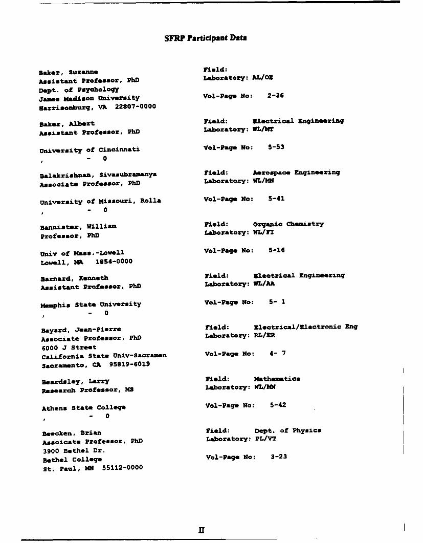
SFRP Participant Data
Baker, Susanne Field:
Assistant professor, PhD Laboratory: AL/03
Dept. of PsychologyJames Madison University Vol-Page No: 2-36
gazrisonburq, VA 22807-0000
Baker, Albert Field: Electrical mngineering
Assistant Professor, PhD Laboratory: WL/MT
University of Cincinnati Vol-Page No: 5-53
- 0
Balakrishnan, SivasubramAnYa Yield: Aerospace Engineering
Associate Professor, PhD Laboratory: WL/HO
University of Missouri, Rolla Vol-Page No: 5-41
- 0
Bannister, William Field: Organic Chemistry
professor, PhD Laboratory: WL/FI
Univ of Mass.-Lowell Vol-Page No: 5-16
Lowell, za 1854-0000
Barnard, Kenneth Field: Electrical Enqineering
Assistant Professor, PhD Laboratory: WL/Ah
M4emphis State University Vol-Page No: 5- 1
- 0
Bayard, Jean-Pierre Field: EZlectrical/Electronic Eng
Associate Professor, PhD Laboratory: RL/ER
6000 J streetCalifornia State Univ-Sacramen Vol-Paqe No: 4- 7
Sacramento, CA 95819-6019
Beardsley, Larry Field: Mathematics
Research Professor, MS Laboratory: WL/W
Athens State College Vol-Page No: 5-42
- 0
Beecken, Brian Field: Dept. of Physics
Assoicate Professor, PhD Laboratory: PL/VT
3900 Bethel Dr.
Bethel College Vol-Paqe No: 3-23
St. Paul, iH 55112-0000
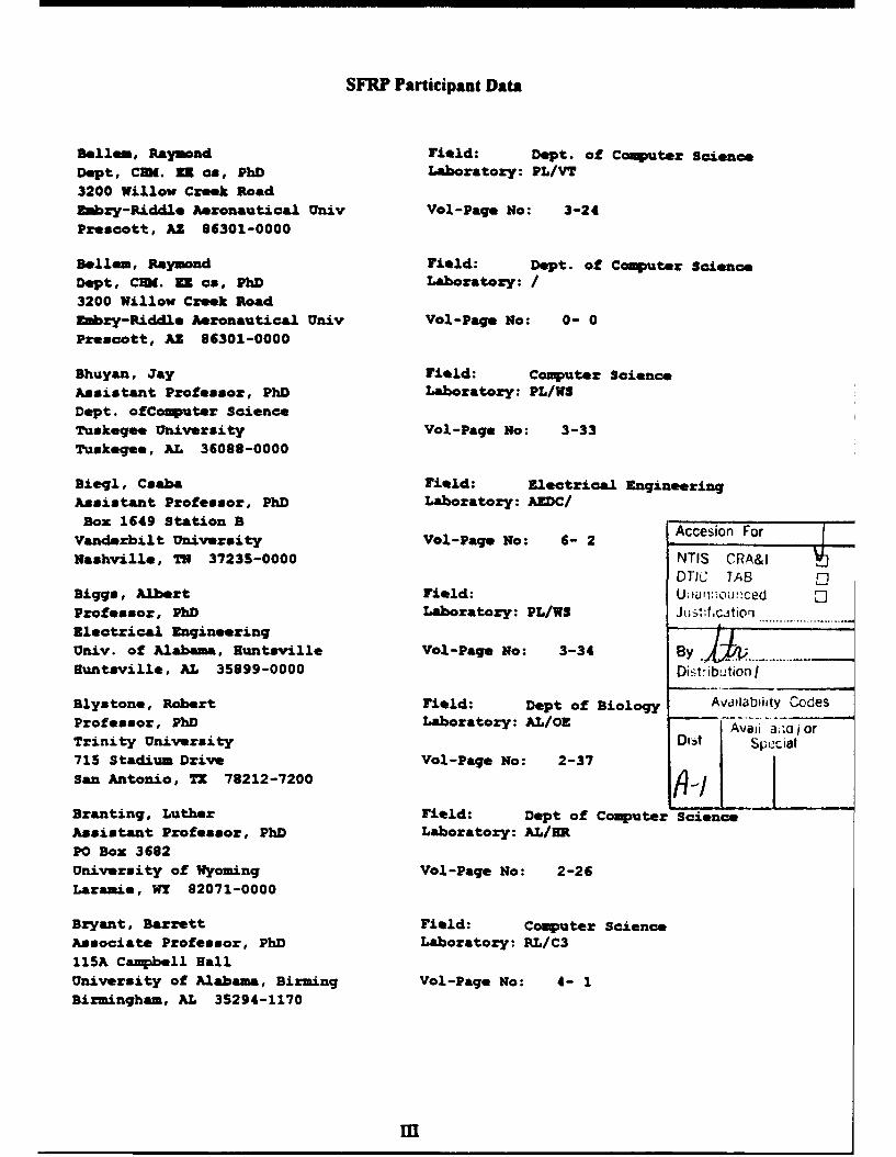
SFRP Participant Data
Bellem, Raymond Field: Dept. of Computer Science
Dept, CUM. 13 ca, PhD Laboratory: PL/VT3200 Willow Creek RoadZmbry-Riddle Aeronautical Univ Vol-Page No: 3-24Prescott, AZ 86301-0000
Bellem, Raymond Field: Dept. of Computer ScienceDept, CUM. UR ca, PhD Laboratory: /3200 Willow Creek RoadEmbry-Riddle Aeronautical Univ Vol-Page No: 0- 0
Prescott, AZ 86301-0000
Bhuyan, Jay Field: Computer ScienceAssistant Professor, PhD Laboratory: PL/WSDept. ofComputer ScienceTuskegee University Vol-Page No: 3-33Tuskegee, AL 36088-0000
Biegl, Csaba Field: Electrical EngineeringAssistant Professor, PhD Laboratory: AEDC/
Box 1649 Station 8Vanderbilt University Vol-Page No: 6- 2 Accesion ForNashville, TN 37235-0000 NTIS CRA&I
DTJC TAB DBiggs, Albert Field: U;wr•,:-.Ou:cedProfessor, PhD Laboratory: PL/WSElectrical EngineeringUniv. of Alabama, Huntsville Vol-Page No: 3-34 ByHuntsville, AL 35899-0000 Dist.ibution I
Blystone, Robert Field: Dept of Biology Availabtiity CodesProfessor, PhD Laboratory: AL/Ol vj-i. ~djoTrinity University Dist Spccial715 Stadium Drive Vol-Page No: 2-37San Antonio, TX 78212-7200 f/
Branting, Luther Field: Dept of Computer ScienceAssistant Professor, PhD Laboratory: AL/HRPO Box 3682University of Wyoming Vol-Page No: 2-26Laramie, WY 82071-0000
Bryant, Barrett Field: Computer ScienceAssociate Professor, PhD Laboratory: RL/C311SA Campbell HallUniversity of Alabama, Birming Vol-Page No: 4- 1Birmingham, AL 35294-1170
m

SFRP Participant Data
Callens, Jr., Eugene Field: Aerospace Engineering
Assocition Professor, PhD Laboratory: WL/Nm
IndustrialLouisiana Technical University Vol-Page No: 5-43
Ruston, LA 71270-0000
Cannon, Scott Field: Computer Science/siophys.
Associate Professor, PhD Laboratory: PL/VT
Computer ScienceUtah State University Vol-Page No: 3-25
Logan, UT 84322-0000
Carlisle, Gone Field: Killgore Research Center
Professor, PhD Laboratory: PL/LI
Dept. of PhysicsWest Texas State University Vol-Page No: 3- 8
Canyon, TX 79016-0000
Catalano, George Field: Department of Civil &
Associate Professor, PhD Laboratory: AEDC/
Mechanical EngineeringUnited States Military Academy Vol-Page No: 6- 3
West Point, MY 10996-1792
Chang, Ching Field: Dept. of Mathematics
Associate Professor, PhD Laboratory: WL/F!
Euclid Ave at 3. 24th StCleveland State University Vol-Page No: 5-17
Cleveland, OH 44115-0000
Chattopadhyay, Somnath Field: Mechanical Engineering
Assistant Professor, PhD Laboratory: PL/RK
University of Vermont Vol-Page No: 3-14
Burlington, VT 5405-0156
Chen, C. L. Philip Field: Electrical Engineering
Assistant Professor, PhD Laboratory: WL/ML
Computer Science Engineer
Wright State University Vol-Page No: 5-26
Dayton, OH 45435-0000
Choate, David Field: MathematicsAssoc Professor, PhD Laboratory: PL/LI
Dept. of MathematicsTransylvania University Vol-Page No: 3- 9
Lexington, KY 40505-0000
IV

SFRP Participant Data
Chubb, Gerald Field: Dept. of Aviation
Assistant Professor, PhD Laboratory: AL/HR
164 W. 19th Ave.
Ohio State University Vol-Paqe No: 2-27
Columbus, OH 43210-0000
Chuong, Chenq-Jen Field: Biomedical Engineering
Associtae Professor, PhD Laboratory: AL/CF
501 W. 1st Street
University of Texas, Arlington Vol-Paqe No: 2- 6
Arlington, TX 76019-0000
Citera, Maryalice Field: Industrial Psychology
Assistant Professor, PhD Laboratory: AL/CF
Department of Psychology
Wright State University Vol-Paqe No: 2- 9
Dayton, OH 4-5435
Collard, Jr., Sneed Field: BiologyProfessor, PhD Laboratory: AL/EQ
Ecology & Evolutionary BiUniversity of West Florida Vol-Paqe No: 2-19
Pensacola, FL 32514-0000
Collier, Geoffrey Field: Dept of Psychology
Assistant Professor, PhD Laboratory: AL/CF
300 College St., NESouth Carolina State College Vol-Page No: 2-10
Orangeburg,, SC 29117-0000
Cone, Milton Field: Electrical Engineering
Assistat Professor, PhD Laboratory: WL/AA
3200 Willow Creek RoadEmbry-Riddel Aeronautical Univ Vol-Page No: 5- 2
Prescott, AZ 86301-3720
Cundari, Thomas Field: Department of Chemistry
Assistant Professor, PhD Laboratory. PL/RK
Jim Smith BuildingMemphis State University Vol-Page No: 3-15
Memphis, TN 38152-0000
D'Agostino, Alfred Field: Dept of Chemistry
Assistant Professor, PhD Laboratory: WL/ML
4202 E Fowler Ave/SCA-240University of South Florida Vol-Page No: 5-27
Tampa, FL 33620-5250
V

SFRP Participant Data
Dag, Asesh Field: Concurrent Engineering
Assistant Professor, PhD Laboratory: AL/HR
Research Center
West Virginia University Vol-Paqe No: 2-26
Morgantown, WV 26505-0000
DeLyser, Ronald Field: Electrical Enqineerinq
Assistant Professor, PhD Laboratory: PL/WS
2390 S. York Street
University of Denver Vol-Page No: 3-3S
Denver, CO 80208-0177
DelVeochio, Vito Field: Biochemic•l Genetics
Professor, PhD Laboratory: AL/AO
BiologyUniversity of Scranton Vol-Page No: 2- 1
Scranton, PA 18510-4625
Dey, pradip Field: cequter Science
Associate Professor, PhD Laboratory: RL/IR
Hamton university Vol-Page No: 4-16
- 0
Ding, Zhi, Field: Electrical Engineering
Assistant Professor, PhD Laboratory: WL/WA
200 Broun Hall
Auburn University Vol-Page NO: 5-44
Auburn, AL 36849-5201
Doherty, John Field: Electrical Engineering
Assistant Professor, PhD Laboratory: RL/OC
201 Coover Hall
Iowa State University Vol-Page No: 4-21
Ames, IA 50011-1045
Dolson, David Field: Chemistry
Assistant Professor, PhD Laboratory: WL/PO
Wright State University Vol-Page go: 5-56
- 0
Dominic, Vincent Field: leoctro Optics Program
Assustant professor, MS Laboratory: WL/ML
300 Colleqe Park
University of Dayton Vol-Page No: 5-28
Dayton, OR 45469-0227
VI

SFRP Participant Data
Donkor, Eric Field: Electrical EngineeringAssistant Professor, PhD Laboratory: RL/OCEngineeringUniversity of Connecticut Vol-Page No: 4-22
Stroes, CT 6269-1133
Driscoll, Jam Field: Aerospace EngineeringAsiociate Professor, PhD Laboratory: WL/PO
3004 FM Bldg 2113University of Michigan Vol-Page No: 5-57Ann Arbor, NJ 40109-0000
Duncan, Bradley Field: Electrical EngineeringAssistant Professor, PhD Laboratory: WL/A
300 College ParkUniversity of Dayton Vol-Page No: 5- 3Dayton, OH 45469-0226
Ehrhart, Lee Field: Electrical EngineeringInstructor, MS Laboratory: RL/C3
Comunications & IntelligGeorge Mason University Vol-Page No: 4- 2
rairfaz, VA 22015-1520
zwert, Daniel Field: PhysiologyAssistant Professor, PhD Laboratory: AL/AOElectrical EngineeringNorth Dakota State University Vol-Page No: 2- 2Fargo, IN 5105-0000
Ewing, Mark Field: Engineering MechanicsAssociate Professor, PhD Laboratory: PL/SX
2004 Learned Halluniversity of Kansas Vol-Paqe No: 3-22
Lawrence, KS 66045-2969
Foo, Simon Field: Electrical EngineeringAssistant Professor, PhD Laboratory: WL/lU
College of EngineeringFlorida State University Vol-Page No: 5-45
Tallahessee, FL 32306-0000
Frantziskonis, George Field: College of Engrng/MinesAssistant Professor, PhD Laboratory: WL/ML
Dept of Civil Engrng/MechUniversity of Arizona Vol-Page No: 5-29
Tuson, AZ 85721-1334
V11
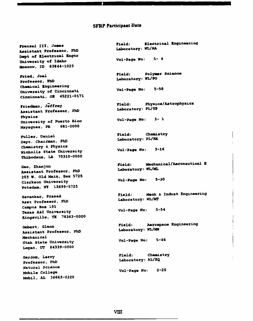
SFRP Participant Data
Frenzel III, Jemes Field: gleotrical Rngineering
Assistant Professor, PhD Laboratory: ilL/AA
Dept of Electrical Znqnr
University of Idaho Vol-Paqe No: 5- 4
Moscow, ID 83844-1023
Fried, Joel Field: Polymr Science
Professor, PhD Laboratory: WL/PO
Chemical EngineeringUniversity of Cincinnati Vol-Page No: 5-58
Cincinnati, OH 45221-0171
Fria~bn, Jeffrey Field: Physics/Astrophysics
Assistant Professor, PhD Laboratory: PL/GP
PhysicsUniversity of Puerto Rico Vol-Page No: 3- 1
Mayaguez, PR 681-0000
Fuller, Da0iel Field: Chemistry
Dept. Chairman, PhD Laboratory: PL/RK
Chemistry A Physics
Nicholls State University Vol-Page No: 3-16
Thibodaux, LA 70310-0000
Gao, Zhanjun Field: Mechanical/Aeronautical E
Assistant Profefsor, PhD Laboratory: WL/1L
203 W. Old Main, Box 5725
Clarkson University Vol-Page No: 5-30
Potsdam, NY 13699-5725
Gavankar, Prasad Field: Mech a Indust Engineering
Asat Professor, PhD Laboratory: WL/MT
Campus Box 191
Texas A&Z University Vol-Page No: 5-54
Kingsville, TX 78363-0000
Gebert, Glenn Field: Aerospace Engineering
Assistant Professor, PhD Laboratory: WL/Ifi
MechanicalUtah State University Vol-Page No: 5-46
Logan, UT 84339-0000
Gerdom, Larry Field: Chemistry
Professor, PhD Laboratory: AL/EQ
Natural ScienceMobile College Vol-Page No: 2-20
Mobil, AL 36663-0220
VM

SFRP Participant Data
Ghajar, Afshin Field: Mechanical Engineeri
Professor, Ph Laboratory: WL/PO
Mach. & Aerospace Engine.Oklahoma State University Vol-Page No: 5-59
Stillwater, OK 74076-0533
Gopalan, Kaliappan Field:
Associate Professor, PhD Laboratory: AL/CF
Dept of EngineeringPurdue University, Calumet Vol-Page No: 2-11
Hammond, IN 46323-0000
Gould, Richard Field: Mechanical Engineering
Assistant Professor, PhD Laboratory: UL/PO
Mechanical & Aerospace EnN.Carolina State University Vol-Page No: 5-60
Raleigh, NC 27695-7910
Gowda, Raghava Field: Computer Information Syn.
Assistant Professor, PhD Laboratory: WL/AA
Dept of Computer ScienceUniversity of Dayton Vol-Page No: 5- 5
Dayton, OH 45469-2160
Graetz, Kenneth Field: Department of Psychology
Assistant Professor, PhD Laboratory: AL/HR
300 College ParkUniversity of Dayton Vol-Page No: 2-29
Dayton, OH 45469-1430
Gray, Donald Field: Dept of Civil Engineering
Associate Professor, PhD Laboratory: AL/EQ
PO Box 6101West Virginia Unicersity Vol-Page No: 2-21
Morgantown, WV 20506-6101
Green, Bobby Field: Electrical Engineering
Assistant Professor, MS Laboratory: WL/FI
Box 43107Texas Tech University Vol-Page No: 5-18
Lubbock, TX 79409-3107
Grubbs, Elmer Field: Electrical Engineering
Assistant Professor, MS Laboratory: WL/AA
EngineeringNew Mexico Highland University Vol-Page No: 5- 6
Las Vegas, M4 87701-0000
Ix

SFRP Participant Data
Guest, Joyce Field: Physical Chemistry
Assoiate, PhD Laboratory: WL/ML
Depazr nt of ChemistryUniversity of Cincinnati Vol-Page No: 5-31
Cincinnati, OH 45221-0172
Gumbo, Godfrey Field: Condensed Matter Physics
Professor, PhD Laboratory: WL/EL
Physics & AstronomyUniversity New York Hunters Co Vol-Page No: 5-12
New York, NY 10021-0000
Hakkinen, Ja1o Field: Mechanical Engineering
Professor, PhD Laboratory: WL/FI
207 Jolley HallWashington University Vol-Page No: 5-19
St. Louis, MO 63130-0000
Hall, Jr., Charles Field:
Assistant Professor, PhD Laboratory: WL/F!
Mech a Aerospace Engr.North Carolina Univ. Vol-Page No: 5-20
Raleigh, NC 27695-7910
Hancock, Thomas Field: Educational Psychology
Assistant Professor, PhD Laboratory: AL/HU
Grand Canyon University Vol-Page No: 2-30- 0
Hannafin, Michael Field: Educational Technology
Visiting Professor, PhD Laboratory: AL/HR
305-D Stone Building,3030Florida State University Vol-Page No: 2-31
Tallahassee, FL 3-2306
Helbiq, Herbert Field: Physics
Professor, PhD Laboratory: RL/ER
PhysicsClarkson University Vol-Page No: 4- S
Potsdam, NY 13699-0000
Henry, Robert Field: Electrical Engineering
Professor, PhD Laboratory: RL/C3
Electrical EngineeringUniversity of Southwestern Lou Vol-Page No: 4- 3
Lafayette, LA 70504-3890
x
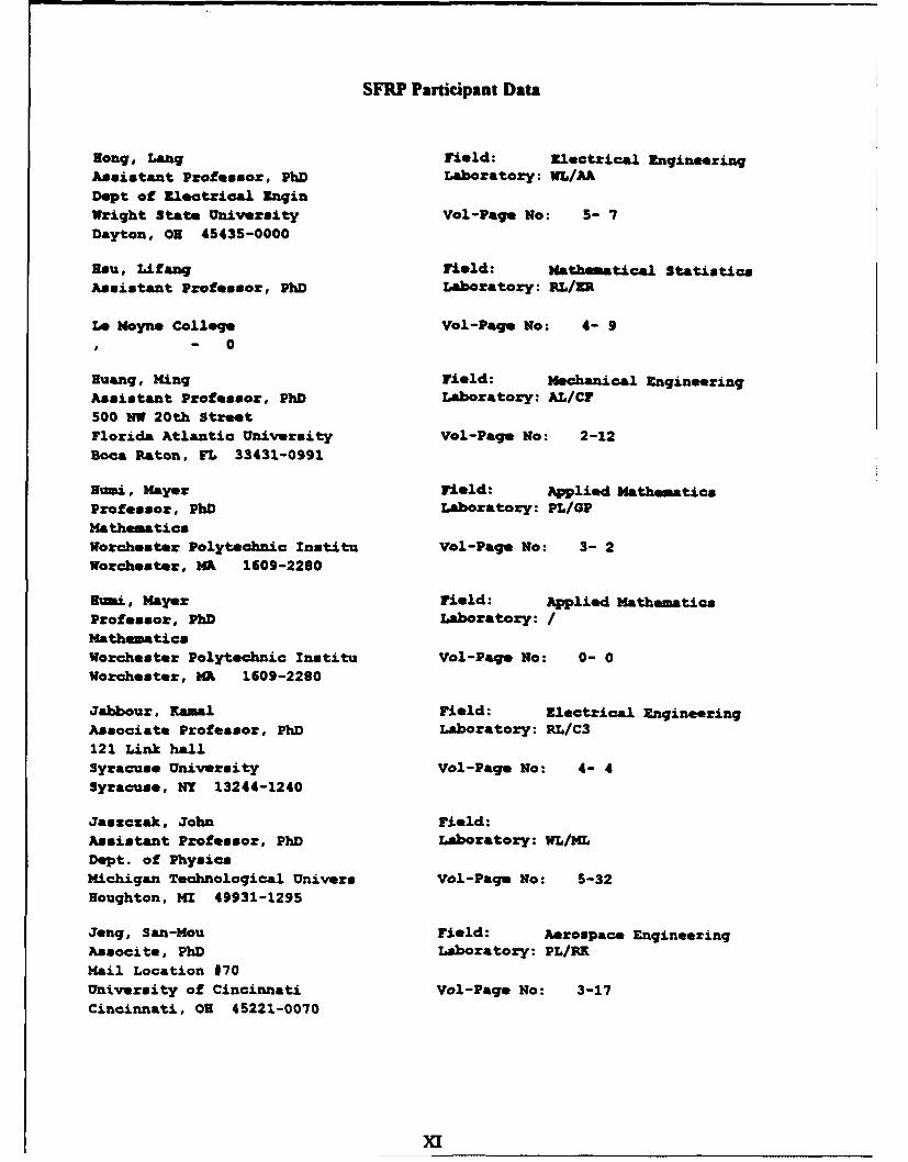
SFRP Participant Data
Hong, Lang Field: Zlectrical EngineeringAssistant Professor, PhD Laboratory: WL/A&Dept of Electrical InginWright State University Vol-Page No: 5- 7Dayton, OH 45435-0000
Rsu, Lifanq Field: Mathematical StatisticsAssistant Professor, PhD Laboratory: RL/EO
Lo Moyne College Vol-Page No: 4- 9- 0
Huang, King Field: Mechanical EngineeringAssistant Professor, PhD Laboratory: AL/CF500 NW 20th StreetFlorida Atlantic University Vol-Page No: 2-12Boca Raton, FL 33431-0991
Humi, Mayer Field: Applied MathematicsProfessor, PhD Laboratory: PL/GPMathematicsWorchester Polytechnic Institu Vol-Page No: 3- 2Worchester, MA 1609-2280
Humin, Mayer Field: Applied MathematicsProfessor, PhD Laboratory: /MathematicsWorchester Polytechnic Institu Vol-Page No: 0- 0Worchester, MR 1609-2260
Jabour, Kamal Field: Electrical EngineeringAssociate Professor, PhD Laboratory: RL/C3121 Link hallSyracuse University Vol-Page No: 4- 4Syracuse, NY 13244-1240
Jaszczak, John Field:Assistant Professor, PhD Laboratory: WL/MLDept. of PhysicsMichigan Technological Univers Vol-Page No: 5-32Houghton, NU 49931-1295
Jeng, San-Mou Field: Aerospace EngineeringAssocite, PhD Laboratory: PL/RXMail Location 170University of Cincinnati Vol-Page No: 3-17Cincinnati, OH 45221-0070
xi

SFRP Participant Data
Johnson, David Field: chemistmy
Associate professor, PhD Laboratory: WL/XL
Dept of ChemistryUniversity of Dayton Vol-Page No: S-33
Dayton, on 45469-2357
Karimi, Amir Field: Mechanical Zngineering
Associate, PhD Laboratory: PL/VT
Division EngineeringUniversity of Texas, San Anton Vol-Page No: 3-26
San Antonio, TX 7024-9065
xheyfets, Arkady Field:
Assistant Professor, PhD Laboratory: PL/VT
Dept. of Mathematics
North Carolina State Univ. Vol-Page No: 3-27
Raleigh, NC 27695-7003
KoblasZ, Arthur Field: Engineering Scince
Associate, PhD Laboratory: AL/AO
Civil KnqineeingGeorgia State University Vol-Page No: 2- 3
Atlanta, GA 30332-0000
Iraft, Donald Field:
professor, PhD Laboratory: AL/Cf
Dept. of Computer Science
Louisiana State University Vol-Page No: 2-13
Baton Rouge, LA 70803-4020
umanr, Rajendra Field: Zlectrtical Engineering
Professor, PhD Laboratory: RL/C3
1250 Bellflower Blvd
California State University Vol-Page No: 4- 5
Long Beach, CA 90840-0000
gunta, Prashant Field: M~ateriels Science
Assistant Professor, PhD Laboratory: WL/ML
Dept of materials Science
Carnegie-Mellon University Vol-Page No: 5-34
pittsburgh, PA 15213-3890
Kuo, Spencer Field: Electrophysics
Professor, PhD Laboratory: PL/GP
Route 110polytechnic University Vol-Page No: 3- 3
ramuinqdale, NY 11735-0000
x~l

SFRP Participant Data
Lakeou, Samuel Field: Electrical Engineering
Professor, PhD Laboratory: PL/VT
Electrical EngineeringUniversity of the District of Vol-Page No: 3-28
Washnington, DC 20008-0000
Langhoff, Peter Field: Dept. of Chemistry
Professor, PhD Laboratory: PL/PK
Indiana University Vol-Page No: 3-18
Bloomington, IN 47405-4001
Lawless, Brother Field: Box 280
Assoc Professor, PhD Laboratory: AL/OK
Dept. Science /MathematicFordham University Vol-Page No: 2-38New York, NY 10021-0000
Lee, Tzesan Field:
Associate Professor, PhD Laboratory: AL/OK
Dept. of MathematicsWestern Illinois University Vol-Page No: 2-39
Mac , IL 61455-0000
Lee, Min-Chang Field: Plasma Fusion Center
Professor, PhD Laboratory: PL/GP
167 Albany StreetMassachusetts Institute Vol-Page No: 3- 4
Cambridge, MA 2139-0000
Lee, Byung-Lip Field: Materials Engineering
Associate Professor, PhD Laboratory: WL/ML
Engineering Sci. & MechanPennsylvania State University Vol-Paqe No: 5-35
University Park, PA 16802-0000
Leigh, Wallace Field: Electrical Engineering
Assistant Professor, PhD Laboratory: RL/ER
26 N. Main St.Alfred University Vol-Page No: 4-10
Alfred, NY 14802-0000
Levin, Rick Field: Electrical Engineering
Research Engineer II, MS Laboratory: RL/ER
EM Effects LaboratoryGeorgia Institute of Technolog Vol-Page No: 4-11Atlanta, GA 30332-0800
xal

SFRP Participant Data
Li, Jian field: Electrical Engineering
Aset Professor, PhD Laboratory: WL/Ah
216 Larsen Hall
University of Florida Vol-Page No: S- a
Gainesville, FL 32611-2044
Lilienfield, Lawrence Field: Physiology & Biophysics
Professor, PhD Laboratory: WNMC/
3900 Reservoir Rd., NWGeorgetown University Vol-Page No: 6-14
Washington, DC 20007-0000
Lim, Tae Field: Meihanxcal/Aerospace ]ngr
Assistant Professor, PhD Laboratory: FJSRL/
2004 Learned Hall
University of Kansas Vol-Page No: 6- 8
Lawrence, RA 66045-0000
Lin, Paul Field: Associate Professor
Associate Professor, PhD Laboratory: WL/FI
Mechanical Engineering
Cleveland State University Vol-Page No: 5-21
Cleveland, OH 4-4115
Liou, Juin Field: Electrical Engineering
Associate Professor, PhD Laboratory: WL/EL
Electrical & Computer Eng
University of Central Florida Vol-Paqe No: 5-13
Orlando, FL 32816-2450
Liu, David Field: Department of Physics
Assistant Professor, PhD Laboratory: RL/ER
100 Institute Rd.
Worcester Polytechnic Inst. Vol-Page No: 4-12
Worcester, MR 1609-0000
Losiewicz, Beth Field: Psycholinguistics
Assistant Professor, PhD Laboratory: RL/IR
Experimental Psychology
Colorado State University Vol-Paqe No: 4-17
Fort Collins, CO 80523-0000
Loth, Eric Field: Aeronaut/Astronaut Engr
Assistant Professor, PhD Laboratory: AEDC/
104 S. Wright St, 321C
University of Illinois-Urbana Vol-Page No: 6- 4
Urbana, IL 61801-0000
XIv

SFRP Participant Data
Lu, Christopher Field: Dept Chemical Engineering
Associate Professor, PhD Laboratory: WL/PO
300 College Park
University of Dayton Vol-Page No: 5-61
Dayton, OH 45469-0246
Manoranjan, Valipuram Field: Pure & AppliedMathmtics
Associate Professor, PhD Laboratory: AL/EQ
Neill HallWashington State University Vol-Page No: 2-22
Pullman, MR 99164-3113
Marsh, Jas Field: Physics
Professor, PhD Laboratory: WL/WH
PhysicsUniversity of West Florida Vol-Paqe No: 5-47
Pensacola, FL 32514-0000
Massopust, Peter Field: Dept. of Mathematics
Assistant Professor, PhD Laboratory: AEDC/
Sam Houston State University Vol-Page No: 6- 5
Huntsville, TX 77341-0000
Miller, Arnold Field:
Senior Instructor, PhD Laboratory: FJSRL/
Chemistry C GeochemistryColorado School of Mines Vol-Page No: 6- 9
Golden, CO 80401-0000
Misra, Pradeep Field: Electrical Engineering
Associate Professor, PhD Laboratory: WL/AA
University of St. Thomas Vol-Page No: 5- 9- 0
Monsay, Evelyn Field: Physics
Associate Professor, PhD Laboratory: RL/OC
1419 Salt Springs RdLe Moyne College Vol-Page No: 4-23
Syracuse, NY 13214-1399
Morris, Augustus Field: Biomedical Science
Assistant Professor, PhD Laboratory: AL/CF
Central State University Vol-Page No: 2-14- 0
xv
SFRP Participant Data
Mueller, Charles rieid: Dept of Sociology
Professor, PhD Laboratory: AL/HI
W140 Seashore Hall
University of Iowa Vol-Page No: 2-32
Iowa City, ZA 52242-0000
Nmurty, Vedula Field: Physics
Associate Professor, MS Laboratory: PL/VT
Texas Southern University Vol-Page No: 3-29
- 0
Zusavi, Mohaiad Field: Elect/Comp. Engineering
Assoc Professor, PhD Laboratory: RL/IR
5708 Harrows Hall
University of Maine Vol-Page No: 4-18
Orono, HE 4469-5708
Naishadham, Krishna Field: Electrical Engineering
Assistant Professor, PhD Laboratory: WL/L
Dept. of Electrical Bng.
Wright State University Vol-Page No: 5-14
Dayton, On 45435-0000
Noel, Charles Field: Dept of Textiles & Cloth
Associate Professor, PhD Laboratory: PL/PZ
1SIA Campbell Hail
Ohio State University Vol-Page No: 3-19
Columbus, O3 43210-1295
Norton, Grant Field: materials Science
Asst Professor, PhD Laboratory: WL/ML
mechanical & Materials En
Washington State University Vol-Page No: 5-36
Pullman, WA 99164-2920
Noyes, Jams Field: Computer Science
Professor, PhD Laboratory: WL/Fz
mathematics a Computer Sc
Wittenberg University Vol-Paqe No: 5-22
Springfield, OH 45501-0720
Nurre, Joseph Field: Mechanical Engineering
Assistant Professor, PhD Laboratory: AL/CF
Else. & Computer Engineer
Ohio University Vol-Page No: 2-15
Athens, OH 45701-0000
SFRP Participant Data
mygren, Thomas Field: Department of Psychology
Associate Professor, PhD Laboratory: AL/Cl
1665 NeAi Ave. MailOhio State University Vol-Page No: 2-16
Columbus, OH 43210-1222
Osterberg, Ulf Field:
Assistant Professor, PhD Laboratory: FJSRL/
Thayer School of Zngrg.Dartmouth College Vol-Page No: 6-10
Hanover, NH 3755-0000
Pan, Ching-Yan Field: Condensed Matter Physics
Associate Professor, PhD Laboratory: PL/WSPhysics
Utah State University Vol-Page No: 3-36Logan, UT 84322-4415
Pandey, Ravindra Field: PhysicsAssistant Professor, PhD Laboratory: FJSRL/
1400 Townsend DrMichigan Technological Univers Vol-Page No: 6-11Houghton, MI 49931-1295
Patton, Richard Field: Mechanical Engineering
Assistant Professor, PhD Laboratory: PL/VT
Mechanical &Nuclear EngineMississippi State University Vol-Page No: 3-30Mississippi State, MS 39762-0000
Peretti, Steven Field:
Assistant Professor, PhD Laboratory: AL/EQ
Chemical EngineeringNorth Carolina State Univ. Vol-Page No: 2-23Raleigh, NC 27695-7905
Petschek, Rolfe Field: Physics
Associate Professor, PhD Laboratory: WL/ML
Department of PhysicsCase Western Reserve Universit Vol-Page No: 5-37
Cleveland, OH 44106-7970
Pezeshki, Charles Field: Mechanical Engineering
Assistant Professor, PhD Laboratory: FJSRL/
Washington State University Vol-Page No: 6-12
Pullman, WA 99164-2920
XVII
SFRP Participant Data
Pepmiier, Edward Field:
Assistant Professor, PhD Laboratory: AL/AO
College of PharmacyUniversity of South Cazolina Vol-Page No: 2- 4
Columbia, SC 29203-0000
Pittaxelli, Michael Field: Information Sye £ Zngr.
AssocLi&te Professor, PhD Laboratory: RL/C3
PO Box 3050, Marcy Campus
SU=T, Institute of Technology Vol-Page No: 4- 6
Utica, My 13504-3050
Potasek, Mazy Field: Physics
Research Professor, PhD Laboratory: WL/I4L
Columbia University Vol-Page No: 5-38
- 0
prasad, Vishwanath Field: Mechanical Engineering
Professor, PhD Laboratory: RL/UR
SENT, Stony Brook Vol-Page No: 4-13
Stony Brook, MT 11794-2300
Priestley, Keith Field: Geophysics
Research Scientist, PhD Laboratory: PL/GP
University of Nevada, Reno Vol-Page No: 3- 5
- 0
Purasinqhe, Rupasiri Field: Dept of Civil Engineering
Professor, PhD Laboratory: PL/PZ
5151 State Univ. Dr.
California State Univ.-LA Vol-Page No: 3-20
Los Angeles, CA 90032-0000
Raghu, Surya field: Mechanical Engineering
Assistant Professor, PhD Laboratory: WL/PO
Mechanical Engineering
SUy, Stony Brook Vol-Paqe No: 5-62
Stony Brook, NY 11794-2300
Ramesh, RiaMsw&My Field: Magement Science/Systems
Associate Professor, PhD Laboratory: AL/Ut
School of Management
Sony, Buffalo Vol-Paqe No: 2-33
Buffalo, NY 14260-0000
xVm
SFRP Participant Data
Ram, Alexander Field:
Professor, PhD Laboratory: AL/CF
MathematiosKansas State University Vol-Page No: 2-17
Manhattan, KS 66506-2602
Ray, Paul Field: Industrial Ingineering
Assistant Professor, PhD Laboratory: AL/OZ
Box 670266University of Alabama Vol-Page No: 2-40
Tuscaloosa, AL 35487-0266
Reimann, Michael Field: Computer Science
Assistant Instructor, HS Laboratory: WL/MT
Information Systems
The University of Texas-Arling Vol-Page No: 5-55
Arlington, TX 76019-0437
Rodriguez, Armando Field: Electrical Engineering
Assistant Professor, PhD Laboratory: WL/lW
Arizona State University Vol-Page No: S-46
Temps, AZ 85287-7606
Rohrbaugh, John Field: Sensors & Applied Electro
Research Engineer, PhD Laboratory: RL/ZR
347 Ferst St
Georgia Institute of Technolog Vol-Page No: 4-14
Atlanta, GA 30332-0800
Roppel, Thaddeus Field: Zlectrical Engineering
Associate Professor, PhD Laboratory: IL/Ml
200 Broun Hall
Auburn University Vol-Page No: 5-49
Auburn, AL 36849-5201
Rosenthal, Paul Field: Mathematics
Professor, PhD Laboratory: PL/RK
Mathematics
Los Angeles City College Vol-Page No: 3-21
Los Angeles, CA 90027-0000
Rotz, Christopher Field: Mechanical Engineering
Associate Professor, PhD Laboratory: PL/VT
Brigham Young University Vol-Page No: 3-31
Provo, UT 84602-0000

SFRP Participant Data
Rudolph, Wolfgang Field: Physics
Associate Professor. PhD Laboratory: PL/LZ
Dept of Physics and AstroUniversity of New Maeico Vol-Page No: 3- 0
Albuquerque, HK 84131-0000
Rudzinaki, Walter Field: Professor
Professor, PhD Laboratory: AL/OK
Dept. of ChemistrySouthwest Texas State Universi Vol-Page No: 2-41
San MazoCo, TZ 76610-0000
Rule, WllUi1 Field: Zngineering Mechanics
Asst Professor, PhD Laboratory: WL/NH
Mechanical Znqineering
University of Alabama Vol-Page No: 5-S0
Tuscaloosa, AL 35487-0278
Ryan, Patricia Field: Electrical Enqineerinq
Research Associate, MS Laboratory: IL/AL
Georgia Tech Research Ins
Georgia Institute of Tech Vol-Page no: S-10
Atlanta, GA 30332-0000
Saiduddin, Syed Field: Physiology/Phaxmncology
Professor, PhD Laboratory: AL/OZ
1900 coffey Rd
Ohio State University Vol-Page No: 2-42
Columbus, O 43210-1092
Schonberg, William Field: Civil & znvironmental
Assoc professor, PhD Laboratory: IrL/aH
Engineering Dept.University of Alabama, Runtsvi Vol-Page No: 5-51
Huntsville, AL 35899-0000
Schulz, Timothy Field: Electrical Engineering
Assistant Professor, PhD Laboratory: PL/LZ
1400 Townsend Dr
Michigan Technological Univers Vol-Page No: 3-11
Houghton, MI 49931-1295
Shen, Mo-Row Field: Aerospace Engineering
Assistant Professor, PhD Laboratory: WL/F!
2036 Neil Ave.Ohio State University Vol-Page No: 5-23
Columbus,, 0 43210-1276
XX

SFRP Participant Data
Sherman, Larry Field: Analytical ChemistryProfessor, PhD Laboratory: AL/OK
Dept. of ChemistryUniversity of Scranton Vol-Page No: 2-43
Scranton, Ph 18510-4626
Shively, Jon Field: Metallurgy
Professor, PhD Laboratory: PL/VT
Civil & Industrial Eng.California State University, N Vol-Page No: 3-32Northridge, CA 91330-0000
Snapp, Robert Field: Physics
Assistant Professor, PhD Laboratory: RL/IR
Dept of Computer ScienceUniversity of Vermont Vol-Page No: 4-19
Burlington, VT 5405-0000
Soumekh, Mehrdad Field: 3lec/Computer ZEngineering
Associate Professor, PhD Laboratory: PL/LI
201 Bell HallSUNY, Buffalo Vol-Page No: 3-12
Amherst, NT 14260-0000
Spetka, Scott Field: Information Sys &Engrg
Assistant Professor, PhD Laboratory: RL/XP
PO Box 3050, Marcy Campus
SUNY, Institute of Technology Vol-Page No: 4-26Utica, NY 13504-3050
Springer, John Field: PhysicsAssociate Professor, PhD Laboratory: AEDCi
Fisk University Vol-Page No: 6- 6- 0
Stevenson, Robert Field: Electrical Engineering
Assistant Professor, PhD Laboratory: RL/IR
Electrical EngineeringUniversity of Notre Daim Vol-Page No: 4-20Notre Dame, IN 46556-0000
Stone, Alexander Field:
Professor, PhD Laboratory: PL/WSMathematics & StatisticsUniversity of New Mexico Vol-Page No: 3-37Alburquerque, 13 87131-1141

SFRP Participant Data
Sveum, Myron Field: Electrical Fngineering
Assistant Professor, MS Laboratory: RL/OC
zlectronic Engineering Te
Metropolitan State College Vol-Page No: 4-24
Denver, CO 80217-3362
Swanson, Paul Field: Electrical Engineering
Research AAsoCict, PhD Laboratory: RL/OC
Electrical Engineering
Cornell University VolPage Mo: 4-25
Ithaca, NY 14853-0000
Swope, Richard Field: Mechanical Engineering
Professor, PhD Laboratory: AL/AO
Engineering Science
Trinity University Vol-Page Mo: 2- 5
San Antonio, TX 78212-0000
Tan, Arjun Field: Physics
Professor, PhD Laboratory: PL/WS
Physics
Alabkam ASM University Vol-Page Mo: 3-38
Normal, AL 35762-0000
Tarvin, John Field: Department of Physics
Associate Professor, PhD Laboratory: AEDC/
800 Lakeshore Drivn
Samnford University Vol-Page No: 6- 7
Birmingham, AL 35229-0000
Taylor. Barney Field: Dept. of Physics
Visiting Assist Professor, PhD Laboratory: WL/ML
1601 Peck Rd.
Miami Univ. - Hamilton Vol-Page No: 5-39
Hamilton, OH 4-5011
This, Y. Field: Physics Dept.
Associate Professor, PhD Laboratory: PL/WS
University of Miami Vol-Page No: 3-39
Coral Gables, FL 33124-0530
Tong, Carol Field:
Assistant Professor, PhD Laboratory: WL/AA
Electrical Engineering
Colorado State University Vol-Page No: 5-11
Fort Collins, CO 80523-0000

SFRP Participant Data
Truhon, Stephen Field: PsychologyAssociate Professor, PhD Laboratory: AL/ZU
Social SciencesWinston-Salem State University Vol-Page No: 2-34Winston-Salmm, NC 27110-0000
Tzou, Horn-Sen Field: Mechanical EngineeringAssociate Professor, PhD Laboratory: WL/FIMechanical EngineeringUniversity of Kentucky Vol-Page No: S-24Lexington, KY 40506-0046
Vogt, Brian Field: Phamaceutical SciencesProfessor, PhD Laboratory: AL/EQ
Bob Jones University Vol-Page No: 2-24- 0
Wang, Xingwu Field: PhysicsAsst Professor, PhD Laboratory: WL/FIDept. of Electrical Eng.Alfred University Vol-Page No: 5-25
Alfred, NY 14802-0000
Whitefield, Philip Field: ChemistryResearch Assoc Professor, PhD Laboratory: PL/LI
Cloud a Aerosol SciencesUniversity of Missouri-Rolla Vol-Page No: 3-13Rolla, NO 65401-0000
Willson, Robert Field: Physics and AstronomyResearch Assoc Professor, PhD Laboratory: PL/GP
Robinson HallTufts University Vol-Page No: 3- 6
Medford, NA 2155-0000
Witanachchi, Sarath Field: Department of PhysicsAssistant Professor, PhD Laboratory: FJSRL/
4202 East Fowler AvenueUniversity of South Florida Vol-Page No: 6-13Tampa, FL 33620-7900
Woehr, David Field: PsychologyAssistant Professor, PhD Laboratory: AL/HRPsycholoogyTexas A&M University Vol-Page No: 2-35College Station, TX 77845-0000
Xx=

SFRP Participant Data
Xtl Longya Frield: Electrical Zngineering
Assistant Professor, PhD Laboratory: WL/PO
Electrical EngineeringThe Ohio state University Vol-Page No: 5-63
columbus, O 43210-0000
Tavuskurt, Savas Field: Mechanical Engineering
Associate Professor, PhD Laboratory: WL/PO
Pennsylvania State University Vol-Page No: 5-64
University Park, PA 16802-0000
Zhang, Xi -Cgeng Field: Physics
Associate Professor, PhD Laboratory: RL/ER
Physics DepartmentRensselaer Polytechnic Institu Vol-Page No: 4-15
Troy, NY 12180-3590
Zhou, Remin Field:
Assistant Professor, PhD Laboratory: WL/HU
Dept. of Elec & Comp. Eng
Louisiana State University Vol-Page No: 5-52
Raton Rouge, LA 70803-0000
Zirmmemann, Wayne Field: Dept Mathematics/Computer
Associate Professor, PhD Laboratory: PL/WS
P.O. sox 22865Texas Woman's University Vol-Page No: 3-40
Denton, TX 76205-0865
XMaV

ANALYTICAL METHODS FOR THE DETERMINATION
OF WEAR METALS IN PERFLUOROPOLYALKYLETHER LUBRICATING OILS
David W. Johnson
Associate Professor
Department of Chemistry
University of Dayton
300 College Park
Dayton, OH 45469-2357
Final Report for:
Summer Faculty Research Program
Wright Laboratory
Sponsored by:
Air Force Office of Scientific Research
Bolling Air Force Base, Washington, D.C.
December, 1993
33-1

ANALYTICAL METHODS FOR THE DETERMINATION
OF WEAR METALS IN PERFLUOROPOLYALKYLETHER LUBRICATING OILS
David W. JohnsonAssociate Professor
Department of ChemistryUniversity of Dayton
Abstract
Analytical methods for the determination of wear metals in
perfluoropolyalkylether lubricants have been developed. Inductively
coupled plasma atomic emission spectroscopy (ICP-AES) has been
chosen as the analytical technique due to its sensitivity and lack
of serious interferences. The method developed allows for the rapid
determination of 20 metals along with phosphorus and sulfur.
Analytical standards have been prepared using metal complexes of
the 8 diketone 2,2-dimethyl-6,6,7,7,8,8,8-heptafluoro-3u5-
octanedione. These complexes were prepared and characterized prior
to use. The PFPAE lubricants studied include Krytox 143ac and
Fomblin Z. Detection limits for the various metals have been
determined to be in the range of 10-100 parts per billion for the
various wear metals. Detection limits for phosphorus and sulfur are
10 parts per million.
33-2
ANALYTICAL METHODS FOR THE DETERMINATIONOF WEAR METALS IN PERFLUOROPOLYALKYLETHER LUBRICATING OILS
David W. Johnson
INTRODUCTION
Perfluoropolyalkylethers (PFPAE) are being developed by the
Air Force as high temperature lubricants for the next generation of
jet engines. While several PFPAE based lubricants are commercially
available, there are no good analytical methods for the analysis of
metals, due to wear of bearing surfaces in these fluids. Analytical
methods based on techniques such as inductively coupled plasma-
atomic emission spectroscopy (ICP-AES) which are commonly used for
conventional lubricants' fail due to the insolubility of the metal
standards in PFPAE fluids. The goal of this study was to develop
metal standards which are both soluble and stable in PFPAE
lubricants and to develop ICP-AES methods for the determination of
wear metals in the commercial PFPAE lubricants.
Metal complexes for use as standards in wear metal analysis
must be both solulte in PFPAE's to at least 100 ppm metal and
stable over a long period of time (months) in the presence of air.
The presence of a long fluorinated chain as part of the ligand was
expected to provide solubility in the fluorinated oil while the
steric shielding improves the hydrolytic stability of the
complex2 . The ligand of choice was 2,2-dimethyl-6,6,7,7,6,8,8-
heptafluoro-3,5-octanedione (HFOD). These complexes were considered
33-3
because of the known hydrolytic and thermal stability and
solubility in organic solvents of the complexes of rare earth
metals3. Transition metal complexes containing the FOD ligand and
several metals have been previously prepared and have been shown to
thermally stable suggesting that these complexes would make
suitable standards.
In this reports the synthesis and characterization of 15 metal
complexes containing the ligand 2,2-dimethyl-6,6,7,7,8,8,8-
heptafluoro-3,5-octanedione is described. These standards have been
used to determine dissolved metal content in fluorinated oils such
as Krytox 143AC and Fomblin Z exposed to metals and high
temperatures.
Experimental Methods
Synthesis
tris(2,2-dimethyl-6,6,7,7,8,8,8-heptafluoro-3,5-octanedionato)
Aluminum Al(FOD) 3 : Al(FOD) 3 was prepared by adding 8.85g (30 mmol)
of HFOD dissolved in 50 mL CC1 4 to a slurry of 1.34g (9.95 mmol) of
AIC13 in 75 mL CC1 4 . The mixture was refluxed in a hood until HC1
gas was no longer being evolved. After cooling, the volume of the
resulting solution was reduced to 25 mL under vacuum and the
solution placed in the refrigerator overnight. The resulting
crystalline solid was filtered and recrystallized from methylene
chloride.
33-4

tris(2,2-dimethyl-6,6,7,7,8,8,8-heptafluoro-3,5-octanedionato)
iron(III)(Fe(FOD) 3 ), tris(2,2-dimethyl-6,6,7,7,8,8,8-heptafluoro-
3,5-octanedionato) chromium(III)(Cr(FOD)3) and tris(2,2-dimethyl-
6,6,7,7,8,8,8-heptafluoro-3,5-octanedionato)manganese(III)
(Mn(FOD) 3 ): These complexes were prepared by the method described
in the literature4.
2,2-dimethyl-6,6,7,7,8,8,8-heptafluoro-3,5-octanedionato
Complexes of Sodium, Magnesium, Calcium, Barium, Nickel(II),
Copper(II), Zinc, Cadmium, Lead(II) and Mercury(II): These
complexes were prepared by adding 5.92g (20.0 mmol) of 2,2-
dimethyl-6,6,7,7,8,8,8-heptafluoro-3,5-octanedione dissolved in 15
mL methanol to a solution of the appropriate metal nitrate or
chloride (10.0 mmol) dissolved in 25 mL of methanol. An aqueous
solution of sodium hydroxide (5.05 mL of 3.97 M) was slowly added.
During the addition a precipitate formed but on further addition,
redissolved. The resulting solution was poured into 500 mL of
deionized water. The resulting precipitate was filtered and
recrystallized from methylene chloride. The crystalline solid was
dried at 60 C under vacuum for 1 hour and stored in a desiccator.
Yield data and metal analysis is shown in Table 1.
Phosphorus and Sulfur:The commercially available compounds
pentafluorophenylsulfide and tris (pentaf luorophenyl) phosphine were
used as the standards for sulfur and phosphorus.
33-5

Table I. Metal and Thermogravimetric Analysis Data for Metal FODComplexes.
% Metal %H2 0 %Complex %Yield actual actual Residue T1/2
(Calc.) (Caic.)Na(FOD) 56 7.12
(7.23)
Mg(FOD) 2 80 3.91 N.O. 2.16 170(3.96)
Ca(FOD) 2 74 6.08 2.76 0.9 220(6.18) (2.78)
NI(FOD) 2 32 8.76 2.97 1.3 185(8.80) (2.70)
Cu(FOD) 2 38 9.68 N.O. 0.7 160(9.72)
Zn(FOD) 2 82 9.88 N.O. 0.8 205(9.97)
Ba(FOD) 2 76 18.36 2.44 0.1 230(18.42) (2.42)
Cd(FOD) 2 69 15.48 3.90 1.6 215(15.60) (2.50)
Hg(FOD) 2 37 25.08(25.37) (2.28)_
Pb(FOD) 2 39 26.02 N.O. 0.9 185(25.98)
Al(FOD) 3 65 2.94 N.O. 0.1 160(2.96)
V(FOD) 3 40 5.38 N.O. 1.7 195,,__(5.44)
Cr(FOD) 3 43 5.51 N.O. 1.0 155(5.55)
Fe(FOD) 3 51 5.95 N.O. 0.9 165(5.93)
Mn(FOD) 3 47 5.77 N.O., (5.84)
Co(FOD) 3 45 6.19 N.O. 0.8 175(6.24) -
33-6

Degradation Studies
Lubricant degradation in the presence of metals was examined
by sealing weighed samples of various powders or iron wire (0.5 g)
and PFPAE based lubricant (5.0 g) inside pyrex test tubes. The
sealed tubes were weighed, heated at the desired temperature for
the listed time and reweighed. Tubes showing significant weight
loss were discarded. The tubes were opened, 20g of Freon E6 was
added and the samples were filtered through a 0.5 micron filter.
The samples were then ready for analysis by ICP-AES.
Caution: Several of the test tubes developed a
substantial pressure or ruptured during the course of the
experiment. Safety glasses should be used at all times
when handling the test tubes.
Physical Methods
The metal content of the complexes was determined by ICP-AES.
A known mass of complex was dissolved in 1.00g methyl-isobutyl
ketone (MIBK). The resulting solution was mixed with 19.00g of
kerosene for ICP analysis. Standards were prepared from appropriate
Conostan standards in the same solvent as was used for the samples.
Thermogravimetric analysis data was obtained on a Dupont model 2100
thermal analysis system. A heating rate of 10 C/min under an
atmosphere of nitrogen, flowing at 50cc/mmn was used for all
33-7
samples. Infrared spectra for all of the metal complexes were
measured as nujol mulls using a Perkin-Elmer model 283 infrared
spectrophotometer. Fluorine 19 NMR spectra were measures at 56 mHz
using a Varian EM-360L NMR spectrometer. Proton NMR spectra at 270
mHz and carbon 13 NMR spectra at 68.7 mHz were measured using a
JEOL FX270 NMR spectrometer.
Inductively Coupled Plasma-Atomic Emission Spectroscopy
Metal concentrations in PFPAE fluids were measured using a
Jarrell Ash Polyscan 61-E spectrometer. Standards were prepared by
dissolving known masses of each metal FOD complex in Freon E6.
Samples of the PFPAE fluid were mixed with appropriate amount of
the standard solution and Freon E6 in a 1:4 ratio of oil to freon
in order to obtain the various concentrations of standard
solutions. All oil samples were diluted 1:4 with Freon E6 before
analysis. For analysis an RF power of 1750 watts, a nebulizer
pressure of 22 PSI and a pump rate of 80 RPM was used. The samples
were aspirated for a minimum of 45 seconds to insure equilibration
within the plasma.
Results
Synthesis: The synthetic approach to these complexes relies on
the rapid reaction of the FOD- ion with the metal cation and the
insolubility of the resulting complex in aqueous solution. All of
33-8
the complexes were isolated in moderate to good yields as soft
crystalline solids. The complexes prepared in this manner often
precipitate as hydrates, however upon heating at 60 C under vacuum,
most of the complexes dehydrate the give either the anhydrous
complex or a stable monohydrate.
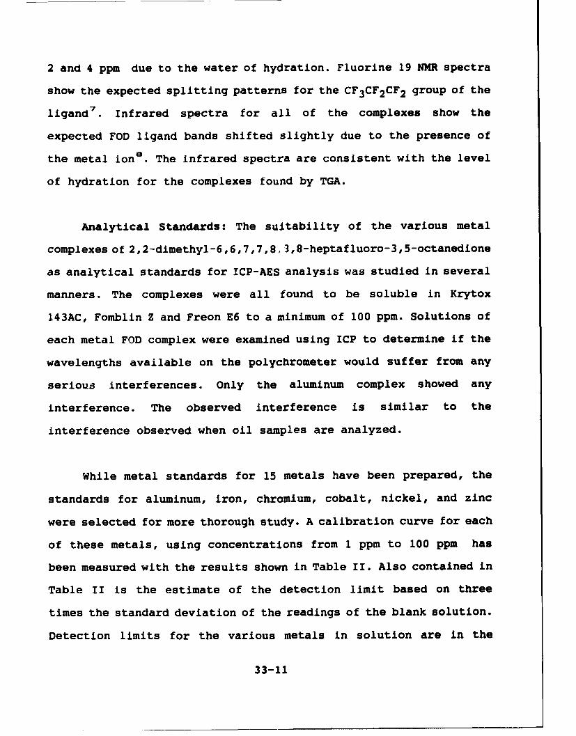
The presence of a single water of hydration in these complexes
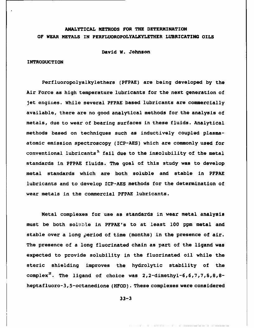
is shown by thermogravimetric analysis. Thermogravimetric analysis
curves for Ca(FOD) 2 "H2 0 and Cu(FOD) 2 are shown in Figure 1. The
curves indicate that these complexes sublime at temperatures of
about 200 C leaving very little residue (<1%). The water of
hydration in the calcium complex is lost first in a well defined
step at about 65 C. The thermogravimetric analysis data for all of
the complexes is given in Table 1. The thermogravimetric analysis
indicates that the calcium, copper and barium complexes described
here are different than the oligomeric complexes reported by
Sievers et.al . The 50 C lowering of the sublimation is consistent
with the lower molecular weight of the monomeric complexes.
The proton NMR spectra of these complexes also serve as an
indicator of the hydration of the complex. The anhydrous complexes
have peaks at 1.1 ppm representing the protons of the t-butyl group
and at 6.1 ppm representing the C-H of the chelate ring6 . The
proton NMR spectrum of the cobalt complex shows splitting of both
peaks due to the two possible isomers for this complex. The proton
NMR spectra of the hydrated spectra show an additional peak between
33-9

W~a: C~t~-U~l~ 'rn File: r4MT.4FaW.UwK~:s:~o.~io sq Ur. operator- ONfJ
"Moodn: Ru 4L&s ~ ~~n Date: 3--Jung.3 .S: 3Co.opent !OC,.%*: TO SOOC. 5oI.CdHI;k IITPOBSI
so-
60-4
20-i
o 4.0 200 300 T 40`0
sie 13.1470 a@ TGA wet-mlatbee T7A ANLYISM am Dast i-tum-a M104Comunt: IOC.'MIE TO S0OC. BOCC/WN.K MZ~h
'40
a 6Too ito 00 --
Figure 1. Thermogravimetric Analysis Curves for A) Ca(FOD) 2 andb) CU(FOD)2
33-10
2 and 4 ppm due to the water of hydration. Fluorine 19 NMR spectra
show the expected splitting patterns for the CF3CF2 CF2 group of the
ligand7. Infrared spectra for all of the complexes show the
expected FOD ligand bands shifted slightly due to the presence of
the metal ion8. The infrared spectra are consistent with the level
of hydration for the complexes found by TGA.
Analytical Standards: The suitability of the various metal
complexes of 2,2-dimethyl-6,6,7,7,8,3,8-heptafluoro-3,5-octanedione
as analytical standards for ICP-AES analysis was studied in several
manners. The complexes were all found to be soluble in Krytox
143AC, Fomblin Z and Freon E6 to a minimum of 100 ppm. Solutions of
each metal FOD complex were examined using ICP to determine if the
wavelengths available on the polychrometer would suffer from any
serious interferences. Only the aluminum complex showed any
interference. The observed interference is similar to the
interference observed when oil samples are analyzed.
While metal standards for 15 metals have been prepared, the
standards for aluminum, iron, chromium, cobalt, nickel, and zinc
were selected for more thorough study. A calibration curve for each
of these metals, using concentrations from 1 ppm to 100 ppm has
been measured with the results shown in Table II. Also contained in
Table II is the estimate of the detection limit based on three
times the standard deviation of the readings of the blank solution.
Detection limits for the various metals in solution are in the
33-11

Table II. Calibration Data and Detection Limits for VariousMetals in Krytox 143AC Diluted 1:4 with Freon E6.5.
Correlation Detection OilElement Coefficient Limit Detection
(ppb) Limit(ppb)
Al 308.2 0.999 44 220
Ba 493.4 1.000 1 5
Cd 228.8 1.000 8 38
Co 228.6 0.994 18 90
Cr 267.7 0.999 32 160
Cu 324.7 1.000 14 71
Fe 259.9 1.000 8 40
Mg 279.5 0.999 2 10
Na 588,9 0.999 20 100
Ni 231.6 0.999 24 120
Zn 213.8 0.999 28 140
range of 1-50 ppb under the conditions of this analysis,
corresponding to concentrations between 5 and 250 ppb in the
original oil sample.
In order for routine analysis of oil samples by ICP-AES to be
practical, several of the analytical standards should be mixed in
a single solution. Table III shows the results of an experiment
where weighed amounts of all six of the complexes were mixed. The
instrument was standardized using the individual solutions of the
six metal ions and then the mixed solution was analyzed. The metal
analysis of the resulting solution shows deviations between 0.5 and
33-12

Table III. Analysis of a Mixed Metal Standard.
Metal Actual 0 Days Dev 7 Days Devppm Found Found
PPM ppm(%RSD) (%RSD)
Al 16.8 16.6 -1.2 16.4 -2.4(0.5) (1.0)
Co 16.6 16.5 -0.6 16.7 +0.6(0.6) (0.8)
Cr 17.7 17.6 -0.6 17.5 -1.2(0.2) (1.1)
Fe 17.5 17.3 -1.1 17.3 -1.1(0.2) (0.9)
Ni 16.4 16.1 -1.8 16.2 -1.2(0.4) (1. )
Zn 21.7 21.5 -0.9 21.4 -1.4(0.4) (0-8)
1.5 %, well within the expected experimental error. The same
solution was analyzed after one week had passed, giving essentially
the same results. The results indicate no reason why several metal
complexes cannot be combined into a single standard solution. The
standard deviation of these determinations is relatively small. The
standard deviation of the analysis of the week old solution is
substantially large, in part due to only a small number (3) of
determinations being made.
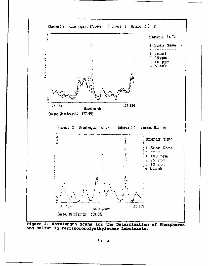
Phosphorus and sulfur were determined using the sequential
portion of the ICP. Based on background scans, the wavelength of
choice for sulfur was determined to be 182 nm and the wavelength of
choice for phosphorus was determined to be 213 nm. Wavelength scans
33-13
Elenent: P Qaveienqth: 177.499 lnterval: I Jindou: 0.3 m
SAMPLE INFO
# Scan Name
1 scanl2 25ppm3 10 ppm"/* blank
177,374 177.624Wauelength
Cursmr Javeenith: I.77.495
,.,. ,SAMPLE INFC,
# Scan Name
.100 ppmS:. 2 25 ppm
'3 10 ppm,4 blank
M t. , n: I
•';e is.r.,t h
Figure 2. Wavelength Scans foz the Determination of Phosphorusand Sulfur in Perfluoropolyalkylether Lubricants.
33-14
for several concentrations of phosphorus and sulfur are shown in
Figure 2. The detection limit based on three times the standard
deviation in the baseline was determined to be 10 ppm for both
phosphorus and sulfur.
Lubricant Degradation Studies
The initial experiments using these metal FOD complexes as
analytical standards was in the analysis of lubricant samples
exposed to high temperatures in the presence of metals. The initial
fluids chosen were Krytox 143AC and Fomblin Z exposed to iron,
chromium and nickel powders at 235 and 290 C for 24 hours. The
liquid contents of the tubes were then analyzed by ICP-AES. The
results of this experiment are shown in Table IV. The results for
any tube which showed a significant change in mass (>0.05 g) are
denoted in Table IV with a *.
In general, Fomblin Z is found to be much more reactive than
Krytox 143AC. Both Krytox 143AC and Fomblin Z were found to react
with chromium to give large chromium concentrations. The samples
where Fomblin Z was in contact with chromium at 290 C were not
analyzed because the decomposition of the fluid generated enough
gas to break the glass tube. The results in Table IV show that iron
and nickel react with the fluids to give small amounts of metal
dissolved in the fluid. Examination of the tubes before opening
gives a visual indication of reaction. The iron samples had a layer
33-15

Table IV. Metal Concentrations in Krytox 143AC and Fomblin ZExposed to Metals at 235 and 290 C.
Metal Fluid Temp. ppm ppm ppmC Fe Cr Ni
Fe Fomblin Z 235 0.01
Fe Fomblin Z 235 0.36*
Fe Fomblin Z 290 0.14
Fe Fomblin Z 290 0.13
Fe Krytox 143AC 235 0.01
Fe Krytox 143AC 235 0.01
Fe Krytox 143AC 290 0.42
Fe Krytox 143AC 290 0.37
Ni Fomblin Z 235 0.47
Ni Fomblin Z 235 1.495
Ni Fomblin Z 290 32.97*
Ni Fomblin Z 290 0.23
Ni Krytox 143AC 235 0.70
Ni Krytox 143AC 235 0.01
Ni Krytox 143AC 290 0.03
Ni Krytox 143AC 290 0.04
Cr Fomblin Z 235 8.1
Cr Fomblin Z 235 6.8
Cr Fomblin Z 290 no liquid for analysis
Cr Fomblin Z 290 '' ''
Cr Krytox 143AC 235 0.23
Cr Krytox 143AC 290 0.35
Cr Krytox 143AC 290 0.34
* A loss of weight greater than 0.05g was seen in this sample.
33-16
of black powder on top of the light gray powder. The composition of
the black solid will be the subject of further investigations.
A second series of experiments where lubricant degradation in
static tests were investigated used various forms of oxidized iron
(Fe 203, Fe 30 4 or FeF 3 ) and iron wire in contact with Krytox 143AC.
Separate samples were heated at 246 and 274 C for 48 hours cooled
nd analyzed by ICP. The results of this experiment are shown in
Table V. The iron wire was found to show very little reaction. The
data indicate that iron oxide (Fe 20 3 or Fe 3 0 4 ) are much more
reactive than iron metal under the conditions of the test.
Iron(III) fluoride (FeF 3 ) is also observed to be quite
reactive towards Krytox 143AC. The test tubes containing FeF3
developed a substantial pressure during the test. When the tubes
were opened the pressure was sufficient to blow the top of the tube
to the ceiling. The FeF 3 powder used in these tubes was observed
to change from a pale green characteristic of FeF 3 to an orange
solid indicating some chemical reaction. The characterization of
these products has not been attempted. The formation of Fek 3 is
thought to be an important step in the degradation mechanism of
PFPAE lubricantss.
33-17

Table V. The Effect of Oxidized Iron Compounds on LubricantReaction.
Sample Fluid Temp Mass of ppm Fe ppm FeSample (a) b
Fe wire Krytox 143AC 246 0.5042 2.29* 6.26*
Fe wire Krytox 143AC 274 0.5041 0.06 0.10
Fe wire Krytox 143AC 274 0.5076 0.02 0.05
Fe wire Krytox 143AC 274 0.5039 0.72 3.50
Fe-O4 Krytox 143AC 274 0.5026 4.40 1.48
FeIOA Krytox 143AC 274 0.5002 0.83 0.43
Fe2OA Krytox 143AC 246 0.5073 0.88 8.19
Fe40 Krytox 143AC 246 0.5022 4.95 10.09
Fe 3 OA Krytox 143AC 274 0.5057 19.08 52.23
FejO 2 Krytox 143AC 246 0.5044 7.15 11.33
Fe.0- Krytox 143AC 274 0.5018 3.54 6.67
Fe 03 Krytox 143AC 246 0.5088 26.89 44.97
Fe,01 Krytox 143AC 274 0.5065 1.69 1.12
Fe 10% Krytox 143AC 274 0.5022 2.16 11.76FeF 3
Fe 10% Krytox 143AC 246 0.5063 2.86 1.47FeF _
Fe 10% Krytox 143AC 246 0.5044 0.77 4.06FeF 3
FeF3 Krytox 143AC 246 0.5041 12.17 39.05
FeF 3 Krytox 143AC 246 0.5018 1.71 17.73
FeF3 Krytox 143AC 274 0.5057 3.72 6.91
FeFIA Krytox 143AC 274 0.5084 2.25(a) The contents of the samples were allowed to settle afterexposure to the high temperature to give analysis results;(b) The contents of the sample were shaken for 15 minutes togive results.
33-18

Conclusions
Several conclusions can be drawn from the data acquired as
part of the AFOSR SFRP program. These conclusions are summarized
below.
1. Metal complexes of 3 diketone 2,2-dimethyl-6,6,7,7,8,8,8-
heptafluoro-3,5-octanedione can be used as metal standards for
the analysis of fluorinated lubricants by ICP-AES. The metal
complexes dissolve in the fluorinated fluids and are
sufficiently stable for their use as standards.
2. Analysis of Krytox 143AC and Fomblin Z indicate that Fomblin
Z is more reactive with iron, chromium and nickel than Krytox
143AC; although both of the fluids react with the three metals
studied.
3. Oxidized iron compounds such as Fe 2 0 3 or FeF3 are much more
reactive than pure iron. It is possible that the observed
reactivity of iron is due to the iron oxide which coats the
surface of the metal.
33-19

References Cited
1. Eisentraut, K.J.; Newman, R.W.; Saba, C.S.; Kauffman, R.E. andRhine, W.E.; Anal. Chem.; 56, 1086A, (1984).
2. Eisentraut, K.J. and Sievers, R.E.; J. Am. Chem. Soc., 87, 5254,(1965).
3. Springer, C.S. Jr., Meek, D.W. and Sievers, R.E. Inora. Chem. 6,1105, (1967).
4. Sweet, T. R. and Brengartner, D. Anal. Chim. Acta, 56, 39,(1974); Kowalski, B.R.; Isenhour, T.L. and Sievers, R.E.; Anal.Chem., 41, 998, (1969).
5. Turnipseed, S.B.; Barkley, R.M. and Sievers, R.E. Inorg. Chem.;'0; 1164 (1991).
j. Kutal, C.; in "Nuclear Magnetic Resonance Shift Reagents"; R.E.Sievers, Ed.; Accademic Press, 1973, 87.
7. Mooney, E.F. "An Introduction to 19F NMR Spectroscopy";Heyden/Sadtler, 1970, p 9-29.
8. K. Nakamoto, "Infrared and raman Spectra of Inorganic andCoordination Compounds", Third Edition, Wiley Interscience, 1978.
9.Carre, D.J.; ASLE Trans.; 29, 121, (1986).;Carre, D.J. andMarkowitz, J.A.; ASLE Trans.; 28, 40, (1985).
33-20

PROCESSING ASPECTS OF GLASS MATRIX, FIBER AND CERAMIC
COMPOSITES FOR ELECTRONIC PACKAGING
Prashant N. Kumta
Assistant Professor
Department of Materials Science and Engineering
Carnegie Mellon University
5000 Forbes Avenue
Pittsburgh, PA 15213
Final Report for:
Summer Research Extension Program
Wright Patterson Laboratory
Sponsored by:
Air Force Office of Scientific Research
Boiling Air Force Base, Washington, D.C.
December 1993
34-1

PROCESSING ASPECTS OF GLASS MATRIX, FIBER AND CERAMIC COMPOSITES
FOR ELECTRONIC PACKAGING
Prashant N. KumtaAssistant Professor
Department of Materials Science and EngineeringCarnegie Mellon University
Glasses and glass-ceramics are well known for their low dielectric constants (e - 3-5) at
1MHz which makes them useful candidate materials as substrates for high speed electronic
packaging. On the other hand crystalline ceramics have moderate dielectric constants (e - 9-12)
at 1MHz while non-oxide ceramics such as AIN and SiC have excellent thermal conductivity
values useful for high power packages. Glass matrix, fiber and glass infiltrated ceramic
composites with interconnected phases therefore, have the potential of displaying optimum
thermal and electric characteristics which could make them useful as substrates for electronic
packaging. Borosilicate-Nicalon fiber-glass composites were fabricated using pressure and
pressureless sintering techniques. At the same time preliminary experiments were conducted to
fabricate composites using SCS fiber and borosilicate glass incorporating tape casting
approaches. Preliminary experiments were also conducted to process porous aluminum nitride
ceramics hot infiltrated with borosilicate glass. Results of optical characterization of the
composites indicate that infiltration of Nicalon cloth with glass is achieved by hot pressing at
1000*C using a pressure of 1000 psi, while the tape casting and lamination approach followed
by sintering is useful for fabricating Nicalon tows and glass composites. On the other hand
aluminum nitride ceramics were fabricated with - 28% interconnected pores. Hot infiltration
yielded - 100 pin penetration of glass into the pores of the nitride ceramic. The paper discusses
the processing aspects of these composites.
34-2

PROCESSING ASPECTS OF GLASS MATRIX, FIBER AND CERAMIC COMPOSITES
FOR ELECTRONIC PACKAGING
Prashant N. Kumta
INTRODUCTION
Advancement in circuit technology and the resultant thrust towards miniaturization of devicesand increasing device density has placed stringent requirements on substrate technology. Theserequirements are based on a large part on attaining excellent heat dissipation and fast signalpropagation. The main heat dissipation mechanism is by thermal conduction, while signalpropagation is based on the velocity of the electric signal given by
where g is the relative magnetic permeability and e is the relative dielectric permittivity of the
material. The substrate materials therefore need to possess excellent thermal conductivity andminimum dielectric constant. As a result, the choice of materials satisfying these criteria isrestricted mainly to ceramics and polymers. The role of ceramic materials as substrates in several
packages such as dual-in-line packages, chip carriers, and pin grid arrays is well known andceramic packaging is becoming one of the most actively pursued areas of research [1-61.
Ceramics have dielectric constants ranging from 4 to 10,000, thermal expansion coefficientsmatching silicon (30x10-7 /C), and display a range of thermal conductivities making them one ofthe best insulators and heat conductors. They even exhibit better heat conduction than aluminummetal. They are also highly refractory materials with excellent temperature stability making themgood materials for hermetic applications. The main drawback of ceramic materials with respect to
packaging is their moderate to high dielectric constant and the high processing temperatures.Research in the development of materials for packaging application has been focussed at achievingobjectives which include lower dielectric constant, lower processing temperatures, thermalexpansion match to silicon, improved thermal conductivity, improved techniques of powerdissipation, multilayer processing and high mechanical strength. The materials that have beenidentified for these purposes have been AIN, BeO, SiC, cubic BN and diamond among the ceramicmaterials, while glasses and glass-ceramics have also been investigated for packaging applicationsbecause of their low dielectric constants[7-16]. Table 1 lists the crystalline ceramic materials ofinterest for electronic packaging. Heat dissipation in devices implementing crystalline ceramics ismainly from the bottom of the device through the substrate itself.
Glass-ceramics with their dielectric constant around 5 and their excellent thermal expansionmatch with silicon coupled with the ability to co-sinter with copper, or gold make them potentiallyone of the best candidate materials for high-performance multilayer ceramic substrates[17). In
34-3

addition, thin film metallization and dielectric material could be easily deposited onto the surface of
these substrates, therefore making them amenable for high performance application. The major
disadvantage of glass-ceramics are their low thermal conductivity which make them poor materials
for heat dissipation in packaging application where the chip is bonded face-in in the cavity up
configuration. However, in the case of the application where the heat dissipation occurs from the
back of the chip, this limitation is largely overcome by external vias and water cooling mechanism
as in the thermal conduction module of IBM[181.
Much of the heat is removed from the back of the silicon chip (flip-chip) by implementing
expensive external cooling modes rather then the substrate itself. From the above it can be seen that
there are basically two different types of packaging technologies to cope with the substrate material
limitations. One geared towards high power devices employing by and large crystalline ceramics
and the other directed towards high speed devices utilizing glass-ceramics. Considerable expenses
are therefore incurred for implementing different package designs and fabrication technologies to
maintain high quality performance. The need for these two technologies could be obviated by a
composite with suitable thermal and dielectric properties.MATERIALS ASELECTION AND MTO LGY
The formation of the composite is contingent on the selection of the glass as the matrix and the
selection of second phase material. The choice of selection is very strongly dependent on the
dielectric and thermal conductivity values of the materials. It is therefore desirable to select two
materials, one with the lowest dielectric constant and the other having a high thermal conductivity.
Among the materials cordierite, borosilicate glasses and glass-ceramics of these two systems have
received the most attention for high speed packaging because of their low dielectric constants.
Other glasses have also been developed which show potentially lower dielectric constants such as
borophosphosilicate glasses researched by Macdowell and Beall[19,20]. However, since
borosilicate glasses have been well studied and considerable information available in the literature
in regards to the processing and electrical and thermal properties it was decided as the material of
choice. From the list provided in Table 1, the choice of high thermal conducting electrically
insulating materials are limited to AIN, SiC, BeO and diamond. AIN is an extremely good choice
over beryllia for high performance packages. Diamond on the other hand is an excellent material
but once again the difficulty in synthesizing fine particles and obtaining a continuous phase limits
its choice. Silicon carbide as seen from Table I has a thermal conductivity of 270 W/m-K, and as a
fiber (Nicalon) is commercially available and has been extensively studied for composite
applications. The ceramic fiber grade however, has a thermal conductivity of 12 W/m-K along the
fiber axis at room temperature and a dielectric constant of 9 at 1MHz. Nicalon was therefore
selected as the second phase for these preliminary studies despite its rather poor thermal
conductivity mainly because of the connectivity issue discussed later. Recently, Ramakrishnan et
34-4

al.[21] have fabricated borosilicate glass matrix-Nicalon fiber composites and have studied their
tensile behavior.
As discussed above, the main goal of the studc' was to fabricate composites with optimum
thermal conductivity and dielectric constant for applications as substrates in electronic packaging.
The properties of such a composite can be predicted to some extent based on certain mathematical
models. There are several models that exist, the one that is most well known is the volume fraction
model[22-241. Based on the empirical rules set by the models, it can be seen that a certain volume
fraction of two different phases could result in an optimum thermal conductivity and dielectric
constant. However, what is important for thermal conductivity is the interconnectivity which the
models do not take into account. Thermal conductivity and dielectric constants in a particular
direction are influenced more by connected rather than dispersed phases. Thus, using ceramicfibers and arranging their geometries can serve to be quite effective in achieving the desired optimal
thermal and electrical properties. The weakness of poor thermal conductivity of most ceramic fibershowever can be solved by coating them with the appropriate material. In such cases, the effective
dielectric and thermal conductivity are more realistically predicted by the percolation theory and the
effective medium theory[25].In regard towards connectivity, one can also envisage the use of thermally conducting
aluminum nitride as a composite material if it is possible to deliberately introduce continuous
porosity. Thus, essentially, this would involve fabricating a two phase material havinginterconnected pores as one phase with thermally conducting aluminum nitride as the second
phase. Initial experiments on sintering of aluminum nitride by Prochazka et al.[26] have indicated
that during heat treatment of the green bodies there is essentially coarsening in absence of
densification. This suggests that the geometry of the interconnected structure remains unchangedwhile the scale increases with temperature. They also performed surface area measurements which
indicate an effective surface to surface transport process operating at relatively low temperatures.
At Wright Patterson, therefore, preliminary experiments were conducted on two aspects. One
based on the fabrication of glass-fiber composite using similar concepts of Button et al.[25] exceptwith the use of glass matrix and high thermal conductivity Nicalon fiber in order to fabricate
composites which could potentially exhibit good optimal dielectric and thermal conductivity. Such
substrates could be essentially used at both low (room temperature) and high temperature (-7001C) devices. The other aspect of the research was to fabricate porous aluminum nitride
compacts and to analyze the compacts for presence of continuous pores. Glass was then infiltratedinto the pores of the compacts.
EXPERIMENTAL PROCEDURE
The experimental section will be divided into two parts one related to the fabrication of glass-
fiber composites and the other related to the processing of porous aluminum nitride.
34-5

A. PROCESSING OF GLASS-FIBER COMPOSITES
Since the thermally conducting phase is the fiber, good interconnectivity in three dimensions
could be envisioned by using a 3-D interwoven cloth. However, considering the preliminary nature
of the work, in order to test the feasibility of the concept, it was decided to use a plain weave
Nicalon 2-D woven cloth from Nippon Carbon Co. Ltd., Japan. The matrix material chosen was a
7760 grade borosilicate glass commercially obtained from Coming. The properties of both these
materials relevant for the present work are shown in Table 2.
Two different approaches were followed in the experiments mainly based on pressure and
pressureless sintering.
I. Tape Casting and Sintering
In this case, the borosilicaie glass powder was initially dispersed into solution using fish oil as
the dispersant. The dispersed glass is then mixed with a binder and a plasticizer to blend the glasswith the binder. The resultant colloidal dispersion is then cast into a 8 mil tape. The tape casting
proced - - followed was similar to that developed by Rollie Dutton at Wright Patterson. The tapes
were wen stripped from the bench and then laminated with the Nicalon cloth. Four different routes
as shown in Figure 1 were followed using the tape casting and sintering technique.
In this route, the tapes were laminated directly with cloth at temperatures of 300°F for 15-30
minutes. The laminated tapes were then sintered using a controlled heat treatment cycle. The first
cycle consisted of heating the tapes to a temperature of 500*C in flowing oxygen at a pressure of
5psi at the rate of 20C/min and holding the samples at the temperature for I h. After the I h hold, the
samples were then heated in vacuum to 880°C (- 50°C above the softening point) at 5°C/min andheld for 1 h and 20min. to initiate and complete the sintering of the composite. The atmosphere was
then switched to argon and the samples were cooled to room temperature using a cooling rate of
2°C/min. At the end of this step, the composites were sectioned and the cross sections observed
using optical microscopy.
Metod 2In this route, the tape casting slurry was vacuum infiltrated into the Nicalon cloth whose sizing
was earlier removed by keeping the cloths at 600°C for 5-15 minutes. The vacuum infiltrated
specimens were then laminated between six 8 mils thick tapes and laminated at 300°F for 30 min.
The laminated tapes were then heated at 20C/min to 5000C in flowing oxygen to remove the
organics. A graphite slab weighing 120g was used as a dead weight in order to facilitate the glass
to flow into the tows of the cloth. After a hold of 80 min., the samples were then heated in vacuum
to 1000°C at 10*C/min and held for 80 min. The composite specimens were held at 1000°C for 80
min. after which the samples were cooled very slowly at 20C/min under an atmosphere of argon to
500°C and kept there for atleast 3-Shrs before cooling the samples down to room temperature at
34-6

2*C/min. In another sample, a load of 1O0g was placed on the laminated specimens, while placing
two layers of cloth between tapes for lamination. The samples were then analyzed using optical
microscopy.
Metod 3In this route instead of the 2-D woven cloth experimental trials were conducted using SCS-0
and SCS-6 fiber as the second phase. The fibers were initially rolled onto aluminum foils with a
interfiber distance of 8 mils to form a pre-preg. The pre-pregs were then laminated using 1/8" tape
casted tape at 200°F initially for 5 min. and then applying a very slight load for 10 min. Four pre-
pregs were laminated each between two layers of tape in 0-90 orientation so that a configuration
similar to the 2-D woven cloth could be attained. A final lamination was performed at 250*F for 15
min. initially and then applying a slight load for an additional 15 min. The laminates were then
subjected to a similar heat treatment as described above in methods 1 and 2. Identical procedureswere also followed using SCS-6 fibers.
Mehod 4In this procedure commercially obtained Nicalon tows whose sizing was removed were used as
the second phase. The procedure consisted of initially removing the sizing from the fiber tows at
6000C for 15 min. The tows were then dip coated into the tape casting slurry containing the
borosilicate glass powders. The dip coated tows were then dried in air and then laminated between
four layers of tape using similar procedures as described in 1 and 2. The tapes containing the dip
coated tows were then subjected to an initial burn out at 500*C and then sintered in vacuum at
900*C similar to methods 1 and 2. Similar procedure was also followed using dip coated Nicalon
tows placed in 0-90 orientation except that the sintering was conducted at a temperature of 1000*C.
II. Hot Pressing
This procedure was followed only using the 2-D woven cloth along with the borosilicate glass
powder (7760 grade from Coming). The detailed experimental procedure consisted of the
following steps. The 2-D woven cloth was initially treated for sizing removal at 600'C for - 8-12h.
The clotiis were then vacuum infiltrated with the tape casting slurry. Immediately following the
vacuum infiltration, the wet cloth was placed between two tapes either 8mils or 16 mils thick and
then dried in air. The dried tapes were then laminated between two 8mils or 16 mils thick tapes at
300M F for 10 min. initially and then with a load at 300N F for an additional 10 min. The laminated
samples were then placed in an ashing furnace for removal of organics and binder. The samples
were heated at the rate of 20C/ min to 5000C and kept for 80 minutes after which the temperature
was brought down at 2°C/min. to room temperature. After this treatment, these samples were then
loaded into a die and packed with the glass powder after placing graphoil foils at the bottom and
top of the die cavity. A stacking sequence consisting of alternate layers of glass powder followed
by the cloth was used. Initial experiments consisted of using just the laminated cloth without
34-7

packing any additional glass powder. The experiments were then modified with two layers of cloth
alternating with glass powder. Finally, five layers of laminated cloths were stacked in the die with
alternating layers of glass powder in order to minimize the distance between the cloth layers and
enhance the connectivity.
After the samples were stacked into the die, the die was loaded into the hot press. The system
was then pumped down to 35gtm. The die was then heated to 1000*C in vacuum and then a
pressure of 1500-2000 psi was then applied to the samples. The load was kept constant for - 30
minutes after which the samples were cooled down to room temperature. The samples were then
recovered from the die and observed for glass penetration using optical microscopy.
B. PROCESSING OF POROUS ALUMINUM NITRIDE
The experimental procedure consisted of using commercially obtained aluminum nitride from
Starck chemicals in Germany. The as-received powders were mixed with acetone and cold pressed
into pellets (1/4" thick) and 0.5" in diameter by application of pressure 1000 psi. The cold
pressed pellets were dried overnight and then cold isostatically pressed at 35000 psi. to a final
dimension of 7/32" thickness and 7/16" diameter. The pellets were then placed in a closed graphite
crucible covered with loose aluminum nitride powder. The pellets were then sintered in a static
nitrogen atmosphere of 1 atmospheric pressure. Two sets of experiments were conducted one at
1800-1880*C for one hour. Another set of experiments were conducted on powders that were ball
milled in ethanol for 24h and then cold pressed followed by cold isostatic press to form green
compacts. These compacts were then sintered under identical conditions except at a temperature of
1900-1920 0C for one hour. After the sintering experiments, the samples were polished and
observed under an optical microscope. Meanwhile, glass infiltration experiments were conducted
on both the pellets using the borosilicate glass. The infiltration was conducted by placing the pellets
in a graphite die covered with the 7760 commercially obtained Coming grade glass that was used
in part A. The loaded die was then heated to 10000 C and a pressure of 1500-2000 psi was then
applied for 30 minutes. The sample was then recovered and the cross sections observed under an
optical microscope to observe the glass infiltration.
RESULTS AND DISCUSSION
The report discusses the results of the preliminary trials conducted at Wright Patterson. These
results will be presented in three sections. Section I will discuss the results of the experiments
conducted primarily on tape casting, lamination and sintering of the Nicalon 2-D cloth, the SCS-0
and SCS-6 fibers and on plain Nicalon tows. On the other hand section II will discuss the results
of the work conducted on hot pressing of the Nicalon cloth and the borosilicate glass. Section III
will then discuss the results on the processing of porous aluminum nitride and preliminary trial
conducted on infiltration of the borosilicate glass.
34-8
Section I: Tape Casting and Sintering
Method 1: Tape casting and lamination of 2-D Nicalon cloth followed by sintering
In order to fabricate the composite initial trials were conducted to observe the feasibility of
direct lamination of the Nicalon cloth placed between two 8 mil cast tapes of borosilicate glass. The
tapes with the cloth were laminated and then sintered following the schedule described in the
experimental section. The resulting composite on removal from the furnace was extremely fragile
and would peel off at several places. There was noticeable surface cracks due to thermal stresses.
The samples were cut and mounted on epoxy and then polished following standard ceramic
polishing procedures. The optical micrograph obtained on the cross section of the sample is shown
in Figure 2. The micrograph clearly shows that the glass has only been able to wet just the surface
of the tows without resulting in any penetration at all. This could be because of several reasons.
First, the temperature not being high enough to cause the glass to be sufficiently fluid to penetrate
the fibers. Second, the fiber spacing =lOgnm is too small requiring extremely high capillary
pressures to cause penetration of the glass through the fiber spacing. For example making an
erroneous assumption for the sake of simplicity that the glass possesses the same surface energy as
water (78 dynes/cm) the capillary pressure amounts to 156000 Pa. This suggests the need to
provide for additional on the top of composite during sintering to cause reasonable penetration.
Method 2: Effect of increased temperature, vacuum infiltration and pressure
Based on the above results, it was decided to initiate initial contact between the glass and the
Nicalon fibers by vacuum infiltration. Hence, the Nicalon cloth was initially pretreated to remove
the sizing and then vacuum infiltrated with the borosilicate slurry. After infiltration, the cloth was
placed between two tapes and then laminated. The laminated tape was then heated to a higher
sintering temperature of 1000'C and after the initial hold of 80 minutes was then subjected to a
slow cool (2rC/minute) to 500"C. The composite was held at this temperature for at least 3h before
cooling down to room temperature. In order to induce penetration a dead weight of -120g was
placed on top of the composite. Modification of the initial conditions appeared to cause visible
changes in the composite. Figure 3 shows the cross section of the composite observed under an
optical microscope after routine grinding and polishing. The micrographs clearly show an
improvement over the earlier case in terms of penetration of the glass into the fiber spacing. Since
the two layers of the cloth were laminated after infiltration, the micrographs show the longitudinal
cross section of the fibers also. Although, penetration has improved, there still appears to be
porosity in the glass matrix suggesting possibly the requirement for longer heat treatment in
vacuum. Repeating the procedure once again using a dead weight of 100g however once again
showed considerable porosity in the glass although, there were regions wherein the glass had
penetrated into the fiber spacings.
These experiments therefore suggest that vacuum infiltration combined with a higher
34-9
temperature and use of a dead weight helped to improve the penetration of the glass melt into the
fiber spacing. However, the concept of tape casting and sintering seems to be quite inadequate on
its own to result in a good composite with complete wetting of the glass and the fiber. As
mentioned, one of the main reasons is the high viscosity and the tremendous capillary pressures
that need to be overcome to cause penetration into the fine fiber spacing. On the other hand, it
should be mentioned that the glass powder is quite coarse with an average particle size of -I0Nm.
Thus, vacuum infiltration does not result in adequate penetration into the fiber spacing. However,
the use of a sol-gel derived sol or a much finer glass particle size could result in improved
wettability improving the quality of the composite.
Method 3: Tape casting and lamination of SCS-0 and SCS-6 fiber followed by sintering
These experiments were conducted since the tape casting and sintering approach failed to
provide with an adequate quality composite on which the electrical and thermal properties could be
measured. Initial experiments were conducted using the SCS-0 grade fiber which is essentially non
stoichiometric SiC with excess carbon and some oxygen. The fibers were initially rolled onto a
pre-preg as described in the experimental section and then laminated onto the borosilicate tapes.
Similar sintering procedures were followed as with the 2-D Nicalon cloth. Four layers of the fibers
were placed in 0-90 orientation and laminated following identical procedures as in the case of the 2-
D Nicalon cloth. The composites were heated to 1000*C for sintering and cooled down at
20C/minute to 5000C at which it was kept for almost 4h before cooling down to room temperature.
The composite however, was not at all transparent and appeared dark and unclear as though, there
was unburnt binder trapped inside the composite. The cross section of the composite also revealed
the presence of considerable porosity visible to the naked eye suggesting fiber degradation. This
could possibly because of the diffusion of Na+ from the glass into the interface of the fiber and the
glass causing reaction with the oxygen in the fiber. Similar observations have been cited by Mah et
al.[271 at Wright Patterson using the SCS-0 fibers with sodium containing glass.
In the case of the SCS-6 fibers, once again similar sintering procedure reported for the cloth
was followed. Four layers of the fibers were laminated in 0-90 orientations and then subjected to
sintering after binder burn out at 500"C at 10000C. Figure 4 shows the cross section of the
composite observed under an optical microscope. The micrographs clearly indicate fiber swimming
that has occurred during the sintering process. At the same time considerable porosity is seen
particularly close to the fibers. The SCS-6 fibers are chemically made up of a central carbon core,
an inner coating covering the core, four SiC layers deposited on the inner coating, and an
outermost coating whose composition has long been a controversy[281. However, recently Ning et
al.[281 have reported the results of the microchemical analysis of the SCS-6 fiber. Their studies
indicate that the outermost layers are made up of four different layers of SiC, the Si to C ratio not
being exactly stoichiometric. The porosity could arise from the reaction of the outer core with the
34-10

glass. A possible reaction being that of carbon with sodium oxide to form CO. This can be seen
very clearly in Figure 5.
Method 4: Tape casting and lamination of Nicalon fiber tows followed by sintering
All the above processes with the cloth as well as with pre-pregs of SCS-0 and SCS-6 seemed
to indicate problems of inadequate penetration in the case of the cloth and reaction with the fiber of
the glass in the case of the pre-pregs. It was therefore decided to study and apply the tape casting
and sintering approach to commercially obtained Nicalon tows. The tows were stripped of the
sizing by heating in air at 6000C. They were then dipped into the borosilicate glass slurry. The dip
coated tows were then laminated and sintered following identical processes as those discussed
earlier in method I. Two set of experiments were conducted using the dip coated tows, one in
which the composites were heated to 9000 C and the other in which the composites were heated to
1000°C with the tows arranged in 0-90 orientation. Figure 6 shows the cross section of the
composites observed under an optical microscope. The micrographs clearly indicate very good
wetting of the fiber with the glass in contrast to that in the case of the cloth, although some random
porosity is evident. In the case of the tows arranged in the 0-90 orientation also, it can be seen that
there is good wetting obtained.
Section II. Hot Pressing of the glass and the Nicalon cloth
From the discussion above it can be seen that the tape casting and sintering approach shows
some promise in the case of fabrication of composites using Nicalon tows. On the other hand it is
extremely difficult to achieve good glass penetration into the fiber tows in the case of the Nicalon
2-D cloth. It was clear that in order to achieve penetration there is need for application of pressure
in addition to increasing the temperature. Hot pressing was therefore seen as a solution to the
problem. Several sets of samples were hot pressed in order to obtain the right set of processing
parameters of temperature (1000*C) and pressure (= 1500-2000 psi). The samples were hot
pressed for 30 minutes and then cut, mounted and polished to be observed under the optical
microscope. Figure 7 shows the cross section of a representative composite. The micrograph
clearly shows regions where the glass has completely penetrated the fiber tows in a uniform
fashion. There are very few regions where the glass has not penetrated into the fiber spacing.
Another noticeable effect is the densification of the glass with very minimum porosity. Thus, it
was possible to fabricate uniformly penetrated glass-fiber composite using the hot pressing
technique at a temperature of 1000*C and pressure of 1000 psi. Following this success, it was
decided to fabricate a composite comprising of five layers of the cloth very closely spaced so that
good connectivity could be achieved for the dielectric measurements.
Section III. Processing of Porous Aluminum Nitride
The as-received aluminum nitride powders were cold pressed and then isostatically pressed to
form a green pellet. The resulting pellets were then sintered in nitrogen at 1900'C for one hour.
34-11

The samples were polished and observed under an optical microscope. Figure 8 shows the optical
micrograph of the polished specimen. As can be seen the micrographs taken at magnifications of
lOOX clearly indicate presence of connected pores continuous on the surface. Densities of the
samples were also measured using Pycnometry which indicated the densities to be 3.257g/cc very
close to the theoretical density. At the same time the apparent density of the samples was calculated
to be 2.32 g/cc. A comparison of the two therefore indicates presence - 28% porosity in the
samples. The fact that there is porosity in the samples and that the pycnometric studies yielded
theoretical density suggests the interconnected nature of pores. These results are extremely
promising particularly for the application in electronic packaging due to the interconnected nature of
the microstructure.
Following on these encouraging results, it was decided to infiltrate the nitride ceramic with the
borosilicate glass. The hot infiltratir-i was conducted at 1000*C and a pressure of 1500 psi. The
resulting composite was mounted, sectioned, polished and observed under the optical microscope.
Figure 9 shows the cross sections of the polished samples. The micrographs indicate that the glass
has penetrated only to a distance of 75-100 gm. These results therefore suggest the tremendous
potential of these experiments for obtaining a porous AIN ceramic satisfying both the electrical and
thermal requirements. The low penetration of the glass into the ceramic infact could provide the
hermetic seal required for the reliability of the substrate against atmospheric moisture. Future work
will be directed towards measuring the thermal and electrical characteristics of these composites.
CONCLUSIONS
The results of the preliminary studies conducted on processing of glass-fiber and glass-ceramic
composites indicate the extreme difficulty faced in trying to apply the tape casting and sintering
approach particularly, in the case of the 2-D woven fiber cloth. However, the results of the work
suggest the potential of this approach for processing of composites using slurry coated Nicalon
tows where successful penetration of the tows with the glass was achieved. Substantial fiber
degradation was observed in the case of the SCS-0 fiber due to a possible interaction of glass with
the fiber. However, hot pressing of borosilicate and Nicalon cloth at 1000*C and 1500 psi resulted
in the formation of good composites with successful penetration of the fiber tows with glass. At
the same time preliminary sintering studies conducted on commercially obtained AIN powders
resulted in ceramic with - 28% connected porosity. Hot infiltration of the ceramic provided -75-
IOOlgm penetration of the glass into the connected pores. These results particularly, those with the
AIN are therefore extremely encouraging in terms of the goals of the research and will form a part
of the extension research proposal to be submitted to the AFOSR.
ACKNOWLEDGEMENTS
The author would like to acknowledge the support of the Air Force Office of Scientific
Research for providing support for the summer research. In addition, the author would like to
34-12

thank Drs. Tai-il Mah, Rollie Dutton and Edmund Moore for useful technical assistance. The help
of Kristi Keller, Cathy Gustafson, Charlie Cook, Marlin Cooke, Mark Dodd, George Cornish and
Dennis Petri of UES and all the support staff in the ceramics group at Wright Patterson
Laboratories is also acknowledged. The author would also like to thank Ms. Kim Andrews and
Ms. Cindy Emerick for their help in preparation of samples for characterization. Finally, the author
would like to acknowledge the support of Drs. Ron Kerans, Alan Katz and Paul Jero for providing
the opportunity to participate in the summer faculty program.
REFERENCES
1. 'Microelectronic Packaging Handbook', Edited by R.R. Tummala and E.J. Rymaszewski, VanNostrand Reinhold, New York, (1989).2. G. Geiger, Bulletin American Ceramic society, 69, (1990) 1131.3. E.M. Rabinovich, J. Electronic Packaging, 111, (1989) 183.4. R.R. Tummala and R.B. Shaw, High Tech Ceramics, Ed. P. Vincenzini, Elsevier SciencePublishers B.V. Amsterdam, (1987) 75.5. J.L. Sprague, IEEE Transactions on Components, Hybrids, and Ma turing Technology,13, (1990) 390.6. K.R. Kinsman, J. Metals, 6, (1988) 7.7. N. Kuramoto, H. Taniguchi and I. Aso, Ceramic Bulletin, 68, NO. 4, (1989) 883.8. N. Kuramoto and H. Taniguchi, J. Mater. Sci. Lett.,3, (1984) 471.9. T.B. Troczynski and P.S. Nickolson, J. Amer. Ceram. Soc., 72 [8] (1989) 1488-1491.10. N.S. Van Damme, S.M. Richard and S.R. Wizer, J. Am. Ceram. Soc., 72 [8] (1989) 1409-1414.11. A. Hal, T. Shi, K. Wakimura, Sennan, M. Tonaka. Shimonoseki, Mitsui Toatsu Chem. Inc.Tokyo. Japan,"Method For Preparing Aluminum Nitride And Its Sintering". U.S. Patent No.4869925, (1989).12. U. Klabunde, W. Chester, E.J. Newitt, C. Ford, F.N. Tebbe, H. Del. E.I. DuPont deNemours & Co. Wilmington, Delaware,"Gas Phase Preparation of Aluminum Nitride", U.S.Patent No. 4865830, (1989).13. S.L. Dole, R.H. Arendt, W.D. Pasco, General Electric Co., Schnectady, N.Y., "AlkalineEarth Fluoride Additive For Sintering Aluminum Nitride", U.S. Pat. No. 4843042, (1989).14. S. Kuratani, K. Uno, S. Mizuno, H. Sakuramoto, and S. Nishiyama, Narumichina Corp.,Nagoya, Japan,"Black Sintered Body of Aluminum Nitride And Process For Producing theSame", U.S. Pat. No. 4843038, (1989).15. S. Mizuno, S. Kuratani, K. Uno, H. Sakuramoto, and S. Nishiyama, Narumochina Corp.,Nagoya, Japan,"Sintered Body of Aluminum Nitride", U.S. Pat. No. 4833108, (1989).16. A. Ikegami and T. Yasuda, "High Thermal Conductive SiC Substrate and Its Applications",5th European Hybrid Microelectronics Conference, (1985) 465.17. R.R. Tummala, J. Am. Ceram. Soc. 74 (1991) 895.18. A.J. Blodgett, Jr., Scientific American, 249 (1983) 2.19. J.F. MacDowell, G.H. Beall, Proc. of the 1st International Science and Technologyconference, "Materials and Processes for Microelectronic Systems", Ceramic Transactions, Ed.K.M. Nair, R.Pohanka and R.C. Buchanan, Vol. 15 (1989) 259.20. J.F. MacDowell and G.H. Beall, Mat. Res. Soc. Symp. Proc.,"Advanced ElectronicPackaging Materials", Ed. A.T. Barfknecht, J.P. Partridge, C.J. Chen and Che-Yu Li, Vol. 167(1989).21. V. Ramakrishnan and N. Jayaraman, J. Materials Science 27 (1992) 2423.22. W.D. Kingery, H.K. Bowen and D.R. Uhlmann,'Introduction to Ceramics', John
34-13

Wiley & Sons, Second Edition, (1976) 635.23. A.J. Moulson and J.M. Herbert,'Electroceramics, Materials, Properties and Applications',Chapman and Hall (1990) 79.24. L.E. Cross and T.R. Gururaja, Mat. Res. Soc. Symp.,"Electronic Packaging MaterialsScience 11", Eds. K.A. Jackson, R.C. Pohanka, D.R. Uhlmann and D.R. Ulrich, Vol. 72 (1986).25. D.P. Button, B.A. Yost, R.H. French, W.Y. Hsu, J.D. Bolt, M.A. Subramanian, H.M.Zhang, R.E. Giedd, A.J. Whitaker and D.G. Onn, Advances in Ceramics, Vol. 26,"CeramicSubstrates and Packages for Electronic Applications", Eds. M.F. Yan, K. Niwa, H.M. O'Bryan,Jr., and W.S. Young, American Ceramic Society (1989) 87-105.26. S. Prochazka and C.F. Bobik, Materials Science Research, Vol. 13,"Sintering Processes",Ed. G.C. Kuczynski, Proc. 5th Intnl. Conference on Sintering and Related Phenomena, (1979)321.27. T. Mah, Private Conversation, (1993).28. X.J. Ning, P. Pirouz and S.C. Farmer, J. Amer. Ceram. Soc. 76 (1993) 2033.
34-14
Table 1. Properties of Selected Cetanic Substrate Materials.
Substrae Glass- 90 cubicRoperties AIN SiC O Ceramics Aumina BN
ThermalCQiductivy 230 270 29 5 25 250 2000(W/mK)
Coefficientof 43 37 68 30-42 67 48 35"Tbermal
(20-200 C( xlO7PC )
S8.9 42 6.8 5.0 9.4 7.1 5.6Constant atI MHzII
Flexural Strength 350 420 250 210 2o1Pa) -- _
Table 2. Characteristics of materials selected for the glass-fiber composite
I Glass System
B•Ksilicat gh•s (Coning sadg 7760)
Composition:
silica 70-80%
bown oxide 10-20%
sodium oxide 1- 10%
alumina 1-10%
arsenic oxide < 1%
potassium oxide 1-10%
Properties
Dielectric Constant: 4.5 @ IMHz, 20 C
EL Fiber
Nicalon (2-D) cloth (Plain weave I sq. in.. Nippon Carbon Co. LId., Japan)
Properties
Dielectric Constant: 6.2 @ 1MHz
Thewial Conductivity: 12W/n-K
34-15

Figure 1. Flow sheet showing the different paths followedin the tape casting and sintering approach I
I
- I
~indDtOu wit Vacuum Infiltration of with SCS-0cloh oth and SCS-6 fibre dip cooed nicalon
Figure 2. Optical micrograph showing the polished cross section of glass-fiber (2-D cloth)composite obtained using the tape casting and sintering approach. The micrograph istaken at a magnification of 200X.
34-16
*77,
Figure 3. Optical micrograph showing the polished cross section of glass-fiber (2-D cloth)composite processed using vacuum infiltration and sintered at a higher temperatureusing a dead weight of 120 g. The micrograph shows improved penetration of theglass into the fiber tows. The micrograph is taken at a magnification of 100Xmagnification.
Figure 4. Optical micrograph showing the polished cross section of glass-SCS-6 fibercomposite taken at 400X magnification. The micrographs show fiber swimming andpossible degradation of the outer carbide coating.
34-17
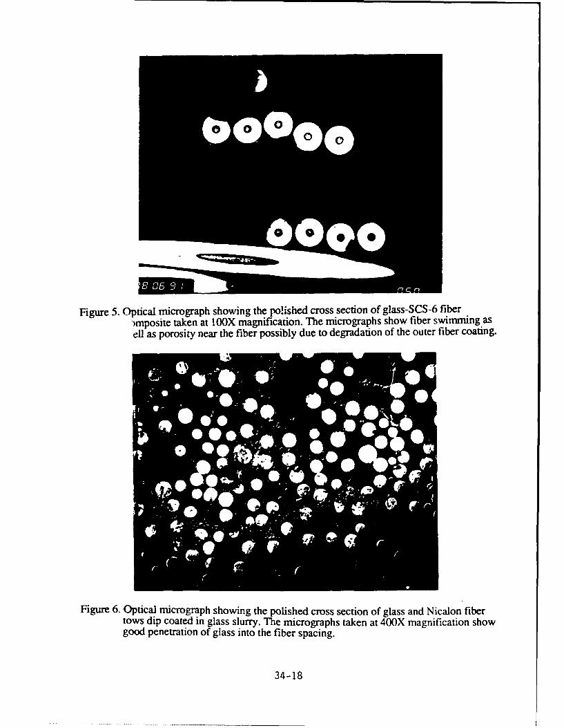
Figure 5. Optical micrograph showing the polished cross section of glass-SCS-6 fiber)mposite taken at 100X magnification. The micrographs show fiber swimming asell as porosity near the fiber possibly due to degradation of the outer fiber coating.
Figure 6. Optical micrograph showing the polished cross section of glass and Nicalon fibertows dip coated in glass slurry. The micrographs taken at 400X magnification showgood penetration of glass into the fiber spacing.
34-18

I. P%
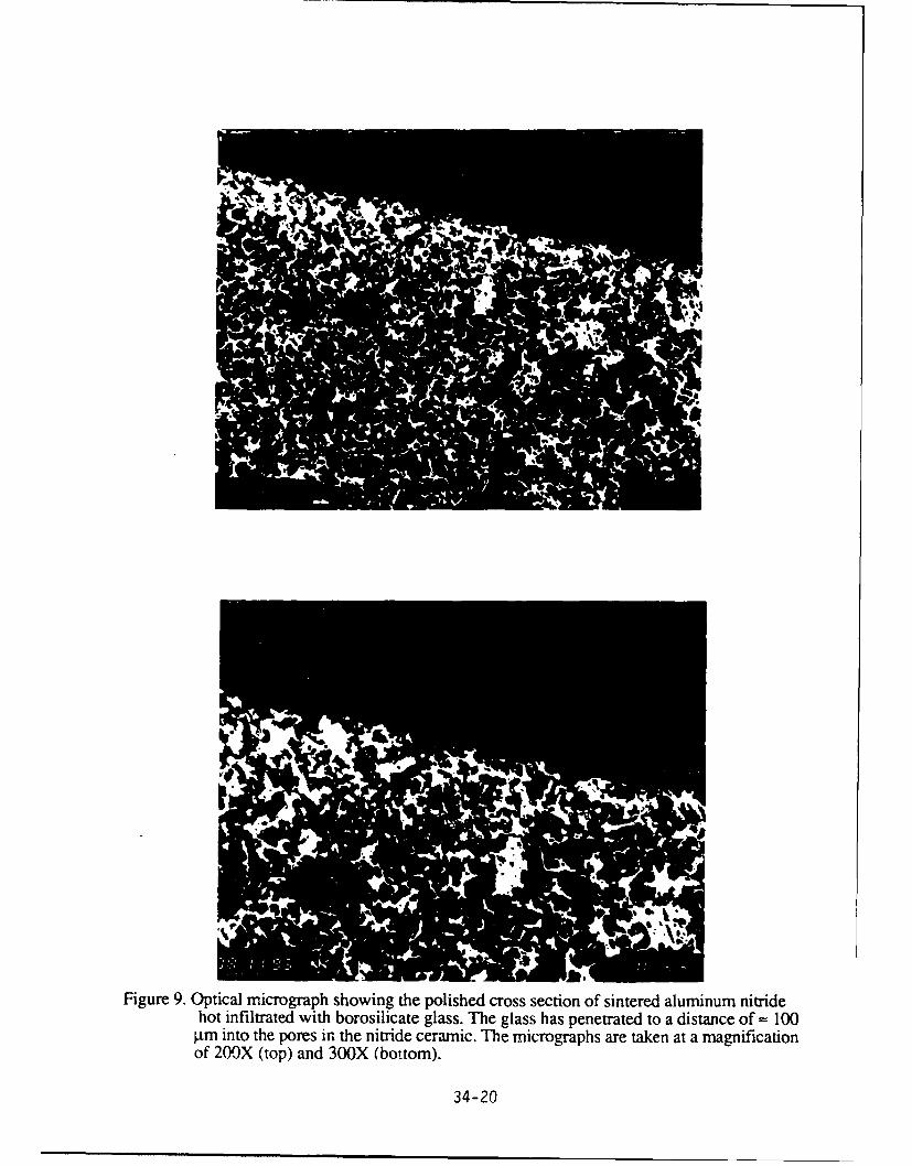
NI
Figure 9. Optical micrograph showing the polished cross section of sintered aluminum nitridehot infiltrated with borosilicate glass. The glass has penetrated to a distance of =100gm into the pores in the nitride ceramic. T'he micrographs are taken at a magnificationof 200X (top) and 30OX (bottom).
34-20

Hydrothermal Effects on the Structural Integrity of
Graphite Fiber-Cyanate Ester Resin Composites
B. L. ("Les") LeeAssociate Professor
Department of Engineering Science and Mechanics
The Pennsylvania State University227 Hammond Building
University Park, PA 16802
Final Report for:Summer Faculty Research Program
Air Force Wright LaboratoryMaterials Directorate, Non-Metallic Materials Division
(USAF Researcher: Capt. Michael W. Holl)
Sponsored by:AIR FORCE OFFICE OF SCIENTIFIC RESEARCH
September, 1993
35-1

INTRODUCTION
Fiber-reinforced polymer matrix composites which form various structural components of
aircraft are subjected to a complex history of temperature, moisture and other environmental
conditions. Their effects, particularly the effects of moisture absorption and thermalcycling, have been extensively studied since the early 1970's [1-9]. Excellent review
articles have been available on these subjects. Among them, worthwhile to note are thereviews done by Springer [4], Adams [5], Ashbee [6], and Wolff [7] on the moisture
effects. Reflecting the state of technology, the past investigations were concentrated in the
epoxy resin matrix composites typically reinforced by graphite, glass or aramid fibers. As
a result, hydrophilic nature of epoxy resins as composite matrices has been well-
documented. Since many applications cannot accept moisture-sensitive nature of epoxy
resin matrix composites, intensive research works were performed to introduce new
thermosetting resins with a reduced tendency of moisture absorption without penalizing the
processability. One important example of the achievement in this direction was the
synthesis of polycyanurate, so-called cyanate ester, resins for composites [7,10,111. Neat
resin casting of cyanate ester was reported to exhibit an equilibrium level of water
absorption as low as 0.7% at 1000C [7].
Cyanate ester resin matrix composites reinforced by glass or aramid fibers established their
presence in the application for multi-layer electric circuit board as early as the late 1970's,
because of the following considerations [ 10]: (a) their glass transition temperatures (Tg)
exceeding those of epoxy resins and matching molten solder temperature (220-270°C); (b)
low dielectric loss properties; and (c) excellent processability (epoxy-like). Recently,
successful efforts for toughening of the resins by the inclusion of elastomer or
thermoplastic secondary-phase have led to a serious consideration of cyanate ester resin
matrix composites for their use in primary structure applications [10, 12-171. Currently
available cyanate ester resins for structural composites offer a desirable combination of high
resistance to moisture absorption, reasonably good fracture toughness, and acceptable
processability. In addition, a relatively low cure temperature (1770C) and a large amount
of free volume after gelation were reported to allow the cure shrinkage less than 1%
creating more residual stress-free composite parts [10].
In the case of epoxy resin matrix composites, moisture absorption was shown to relieve the
residual stresses by matrix swelling and temporarily increase the resistance to
matrix/interface cracking [ 18,19]. The occurrence of this type of interaction is expected to
35-2

be negligible in the cyanate ester resin matrix composites which absorb a very small amount
of water. However, the question of whether this small amount of water absorbed will
eventually influence the fiber-matrix interface of cyanate ester resin matrix composites as in
the case of epoxy resin composites has not been resolved [6,7]. Aside from the issue of
moisture effect on the interfacial adhesion, the structural integrity of cyanate ester resin
matrix composites should be assured under the condition of thermal spike or cycling. Here
a systematic data base is lacking, despite the claims by the resin producers of better
microcrack resistance of cyanate ester resin composites over the epoxy resin composites
upon thermal cycling. One of the first questions to resolve in this area appears to bewhether the effect of thermal cycling can be represented by the cumulative sum of thermal
degradation effect at the peak temperature. An equally important question is what factors
control a critical frequency of thermal cycling above which the deviation from cumulative
effects occurs. These questions were not fully examined even in the case of conventional
thermoset resin matrix composites where extensive data base exists for thermal cycling.
Our study plans to assess the long-term structural integrity of graphite fiber-reinforced
cyanate ester resin matrix composites with a special attention to the issues raised and
discussed so far. As a first step toward this goal, the weight change and the retention of
matrix/interface dependent mechanical properties of the composite systems have been
measured on the exposure to high humidity and thermal cycling respectively. In
consideration of the long-term structural integrity, the study has included the evaluation of
not only static strength but also fatigue lifetime profile of composites. A study has been
initiated to resolve the question of whether the effect of thermal cycling can be represented
by the cumulative sum of thermal degradation effect. Continuing study will eventually
assess cumulative effects of temperature cycling or spike in conjunction with moisture
exposure on the mechanical performance of composites. When completed, the efforts will
to clarify the mechanisms of hydrothermal environment-induced change of the composite
performance, and thereby provide a technical basis for the future work on the
environmental fatigue of composite structures. Preliminary findings of our efforts are
reported in this paper which will be the first one of the series.
35-3

OBJECTIVES
(a) To examine the effects of moisture absorption, temperature cycling, and their
combination on the long-term structural integrity, particularly matrix/interface dependent
mechanical properties, of graphite fiber-reinforced cyanate ester resin matrix composites;
(b) to assess the mechanisms of hydrothermal environment-induced change of the
composite performance; and (c) to provide a technical basis for the future work on the
environmental fatigue of composite structures.
EXPERIMENTS
Specimen Preparation Unidirectional composite prepreg was obtained from ICI
Fiberite Composite Materials Inc. (Tempe, AZ). The reinforcement was Hercules IM7
graphite fiber. The resin matrix for the prepreg was ICI 954-2 cyanate ester resin which
reportedly contains thermoplastic toughener of a proprietary nature. Off-axis angle-plied
laminates were prepared by laying up four prepreg plies with a symmetric configuration of
(+4 5/- 4 53), and curing them in autoclave. The following cure conditions recommended by
the materials supplier were used: heat-up rate of 30C/min; 1 hour at 1210C (2500F)
followed by 2 hours at 1770C (3500F); pressure of 0.69 MPa (100 psi). Some of the
laminates were subjected to an optional postcure cycle consisting of 2 hours at 2320C
(4500F) under contact pressure. The thickness and the resin content of cured composite
panels was approximately 0.57 mm and ??% by weight respectively. Two types of straight
strip specimens were cut with water coo1 ant from the panels: 12.5 mm X 62.5 mm (Type
I), and 18.75 mm X 125 mm (Type II). The specimens were immediately placed in a
desiccator after cutting. Their weights were monitored until they reached an asymptote due
to drying-out of moisture.
Environmental Exposure Both Type I and Type II specimens of graphite
fiber/cyanate ester resin composite were placed for various periods of time in a humidity
chamber which were maintained at 95% RH and 600C (1400F). The weight gain of each
specimen due to moisture absorption was measured in a chemical balance after the moisture
was removed from the specimen surface by soft paper tissue. The results of the specimens
exposed to high humidity continuously were compared with those of the specimens which
were taken out of the humidity chamber for weighing, re-exposed to the humidity, and re-
35-4

weighed. Both techniques produced the same consistent results within the range of data
scattering.
A separate lot of composite specimens were also exposed to dry heat at 1500C (3020F) or
2040C (4000F) in either cyclic or static mode. Static exposure of the composite specimens
to dry heat was performed using an oven without air-circulation. Thermal cycling between
elevated temperature and ambient temperature was accomplished by shuttling the specimen
between the preheated oven and an open area with cooling fan. Shuttling action was
performed using a hydraulic test machine operated at a frequency of 1.67x10⁻³ Hz (10
min/cycle) in a stroke-controlled mode. The above cyclic frequency allowed 5 minutes'
exposure at elevated temperature per each cycle. After the exposure to various
environments described so far, the Type I specimens were used for the measurement of
weight change. The Type II specimens were used for tensile testing in static as well as
dynamic mode.
Mechanical Testing After the exposure to moist heat (95% RH, 600C), dry heat
(150 or 2040C), or thermal cycling (to 150 or 2040C from ambient temperature) for various
periods of time, the Type II specimens of graphite fiber/cyanate ester resin composite were
subjected to static uniaxial tension until failure occurs. The rate of deflection and the initial
gage length of the specimen were 1.25 mm/min and 75mm respectively. The in-plane
shear strength and modulus were defined according to the procedure of ASTM D3518.
Monitoring of strain along the transverse as well as axial direction, which is needed for the
calculation of in-plane shear modulus, was limited to the case of dry specimens. In the
case of axial strain measurement, bonded strain gage technique was used along with an
extensometer. A reasonably close agreement between the two types of measurement was
observed. For wet specimens, only the axial strain was measured by an extensometer.
In the case of dry specimens and the specimens exposed to moist heat (95% RH, 600C) for
50 days, tension-tension fptigue experiments were performed at ambient condition. The
number of cycles to failure were measured at various levels of stress range to define S-N
(stress range vs fatigue life) relationship. Cyclic frequency and the minimum-to-maximum
stress ratio were fixed at 10 Hz and 0.1 respectively. No preventive measure was taken to
reduce moisture desorption of wet specimens during the fatigue experiment.
Failure Analysis Along with mechanical testing, the morphology and the extent of
damage propagation of graphite fiber/cyanate ester resin composites were examined by
35-5

optical microscopy. Scanning electron microscopy (SEM) was used to observe the mode
of failure before and after the exposure to moist heat, dry heat, or thermal cycling. Small
pieces of composite laminates were mounted on specimen studs. The samples were coated
in a sputter coater with a thin layer of gold palladium. The fracture patterns of the coated
samples were examined using the secondary electron mode.
RESULTS AND DISCUSSIONS
Moisture Absorption As discussed previously, the weight change and the retention
of matrix/interface dependent mechanical properties of composites are our immediate and
foremost concern in assessing the long-term structural integrity of graphite fiber-reinforced
cyanate ester resin matrix composites. Our test results clearly showed that IM7 graphite
fiber-reinforced 954-2 cyanate ester resin composites absorb a remarkably small amount of
moisture on the exposure to 95% RH condition at 600C up to 36 days (Figure 1). The
moisture content remained almost constant at a level of around 0.3% by weight after the
initial pick-up within 1 day. Postcured specimens appeared to follow the same trend with a
slightly higher moisture content. These values are comparable to the assumed equilibrium
level of moisture content reported by the materials supplier [10-121. However, a possible
error in our estimation of moisture content cannot be ruled out, mainly because of
extremely low degree of weight change involved and uncertain effectiveness of removing
the moisture absorbed during cutting of the specimen.
One interesting finding was that the degree of moisture absorption undergoes a rather
sudden increase to the level of 1% after the exposure for around 50 days. After this
increase, the moisture content remained constant around 1% up to 100 days' exposure
forming a second level of equilibrium. Even at this level, the moisture content of cyanate
ester resin composite is still lower than that of epoxy resin composites which typically
exhibit an equilibrium moisture content of 1.5 to 1.8% [4]. The observed pattern of
moisture gain, a sudden increase of moisture content after 50 days and the existence of dual
equilibrium levels, clearly indicates that moisture absorption behavior of IM7 graphite
fiber-reinforced 954-2 cyanate ester resin composites cannot be described by a
concentration-dependent form of Fick's law. Moisture diffusion behavior of fiber-
reinforced composites can deviate from Fick's law for the following reasons [41: (a) the
development of cracks or delamination altering the structure of' trial, (b) moisture
35-6

propagation along the fiber-matrix interface, (c) voids in the matrix, and (d) non-Fickian
behavior of matrix itself without defects.
Our microscopy study showed that the composite specimens in dry state are virtually void-
free and well-compacted. However, on the exposure to moist heat (95% RH, 600C) for 50
days, the composite underwent extensive cracking of matrix/interface region (Figure 2).
The damage took the form of not only the delamination between the plies but also
translaminar cracking within the ply. Some matrix cracks remained in the subsurface
region but lying parallel to the plane of surface. Less cracks were observed in the matrix-
rich pockets of composites. The observed damage of matrix/interface region is believed to
be a primary source of a sudden moisture gain after 50 days' exposure. Other potential
sources for anomalous diffusion behavior of cyanate ester resin matrix composites will be
checked in our future work. The question of moisture propagation along the fiber-matrix
interface will be examined by comparing the moisture absorption behavior of the composite
specimens with their edges exposed and that of the specimens with the sealed edges.
Although it is almost certain that the damage of matrix/interface region is responsible for a
sudden moisture gain after 50 days' exposure, the cause of damage formation in the
composites still remains to be answered. As discussed, matrix swelling effect should not
be a factor in the cyanate ester resin matrix composites which initially absorb a very small
amount of water. At the temperature of 600C, the possibility of having the cracks due to
the volume expansion of absorbed moisture is rather slim. Therefore, the only explanation
of the phenomenon is that, on a prolonged exposure to humidity, this small amount of
absorbed water gradually weakens th, matrix interface of cyanate ester resin
composites as in the case of epoxy resin cl .posites. In the case of graphite fiber/epoxy
resin composites, Browning et al [20] showed that matrix/interface dependent 900 strength
of unidirectional lamina decreases by almost 40% at the moisture content of around 1%.
As will be discussed later, in-plane shear strength of our graphite fiber/cyanate ester resin
composites decreased by 20% at the same level of moisture content. Although weakening
of fiber-matrix bonding has been confirmed by subsequent failure analysis, a rather
unusual occurrence of moisture-induced cracks in the absence of external loading is still
difficult to explain. Moisture-induced cracks might be related to the fact that cyanate ester
resins exhibit a large amount of free volume after gelation which led to very low level of
cure shrinkage and residual stresses [10]. More study including chemical analyses of cured
vs postcured composite systems is planned to probe the cause of matrix cracking.
35-7

Moisture Effects on the Mechanical Properties A sudden moisture gain after
50 days' humidity exposure associated with extensive matrix/interface cracking was found
to have direct influences on the static strength and fatigue lifetime profile of IM7 graphite
fiber-reinforced 954-2 cyanate ester resin composites. Static in-plane shear strength of
composites decreased from 70 MPa in dry state to 58 MPa after the humidity exposure. As
shown in Figure 3, S-N (stress range vs the number of cycles to failure) curve of wet
specimens clearlb shifted to the left of that of dry specimens, although the data tended to be
more scattered for the wet specimens. At a given stress amplitude, the composite
specimens which contained extensive cracks as a result of humidity exposure exhibited
almost exponentially shorter fatigue lifetime. When the same data are plotted in log-log
scale (Figure 4), the S-N relationship took the following form of S = a N-b where a and b
are constants. The slope of S-N curve, represented by (-b), were found to be lower for
wet specimens with extensive matrix cracking (-0.045) than dry specimens (-04059).
Past research work [21,221 showed that, when the fatigue lifetime is dominated by the
damage propagation phase, (-b) is equal to (-1/m) where m is a power-law factor of Paris'
law. Fatigue crack growth data for most polymers and composites were reported to followParis' law which takes the following form: da/dN = A(AK)m where a is crack length, N
is cycles, AK is the range of stress intensity factor on each cycle, A and m are constants. If
the above-discussed relationship is valid for our composite system at least in a qualitative
sense, the rate of crack growth at a given range of stress intensity factor should be higher
for the wet specimens (already with extensive matrix/interface cracks initiated) than dry
specimens. This hypothetical conclusion seems to be consistent with the previous
assumption of fiber-matrix interface weakened by absorbed moisture. Separate
experiments involving the measurement of delamination growth under cyclic loading are
planned to verify the relationship between the slope of S-N curve and m factor of Paris
law.
Moisture Effects on Failure Modes Weakening of fiber-matrix interface due to
moisture absorption was confirmed by extensive failure analysis of the composite
specimens based on scanning electron microscopy (SEM). One difficulty in the failure
analysis was the lack of any quantitative means of measuring the extent to which matrix
remnants adhere to the fibers in the crack path region. However, the fracture surface of dry
composite specimens displayed a clear tendency of having the remnant of matrix resin
clinging to the fibers even in a highly-fibrillated region with many bare fibers, as shown in
Figure 5-a. Compared with dry specimens, wet specimens showed a much more reduced
35-8

tendency of having the deposit of matrix resin on the fibers. The frequency of observing
the resin deposit over the given area was found to be distinctly lower for wet specimens.
When observed, the remnants of matrix resin often showed an appearance of being easily
peeled (Figure 5-b).
Thermal Cycling vs Static Exposure In addition to the study of moisture
effects, our research program examined how thermal cycling influences the static strength
of cyanate ester resin matrix composites. The study is intended to be a preliminary phase
of the future investigation which will assess cumulative effects of temperature cycling or
spike in conjunction with moisture exposure on the mechanical performance of composites.
As discussed, one of the first questions to resolve was whether the effect of thermal cycling
can be represented by cumulative sum of thermal degradation effect at peak temperature.
Within this context, the in-plane shear strength of unpostcured laminates of graphite
fiber/cyanate ester resin composites was measured after static exposure at 150 0C as well as
temperature cycling to 1500C for various durations up to 5 days. The in-plane shear
strength of postcured laminates was measured after static exposure as well as cycling to the
heat of 2040C. Both test results were plotted as a function of exposure time at 150 or
2040C. As shown in Figures 6 and 7, the in-plane shear strength of IM7 graphite
fiber/954-2 cyanate ester resin composites decreased steadily on the exposure to dry heat.
The rate of strength degradation on static exposure to heat (about 4% per day) was found to
be close to that of thermal cycling expressed as a function of time at peak temperature. In
the case of postcured specimens, a slight deviation occurred within the range of data
scattering.
From the above test results, it is reasonable to conclude that, at a frequency of 10 main/cycle
and for a relatively short duration, the effect of thermal cycling can be represented by the
cumulative sum of thermal degradation effect at peak temperature. This conclusion was
further supported by the results of ensuing morphology study. The study based on
fluorescent dye-enhanced optical microscopy revealed that any of the specimens subjected
to static heat or thermal cycling do not contain microcracks (Figure 8). Obviously the
degradation of materials occurred at a molecular level. The same mechanisms of strength
degradation can be assumed under static heat as well as thermal cycling. However, the
situation may be altered under thermal cycling condition at higher frequency range and/or
longer durations. Our future program will examine this possibility and, if necessary,
define a critical frequency above which thermal cycling effects deviates from the cumulative
sum of thermal degradation effect at peak temperature.
35-9
CONCLUDING REMARKS
Our study plans to assess the long-term structural integrity of graphite fiber-reinforced
cyanate ester resin matrix composites. As a first step toward this goal, the weight change
and the retention of in-plane shear strength of the composite systems have been measured
on the exposure to high humidity and thermal cycling respectively. Initial test results
clearly showed that cyanate ester resin matrix composites absorb a remarkably small
amount of moisture on the exposure to 95% RH condition at 600C up to 36 days.
Postcured specimens appeared to follow the same trend with a slightly higher moisture
content. One interesting finding was that the degree of moisture absorption undergoes a
rather sudden increase to an equilibrium level of 1 % after the exposure for around 50 days.
The observed pattern of moisture gain clearly indicates that moisture absorption behavior of
graphite fiber/cyanate ester resin composites cannot be described by a concentration-
dependent form of Fick's law.
The morphology study showed that, on the exposure to moist heat for 50 days, the
composite undergoes extensive cracking of matrix/interface region in the form of the
delamination between the plies as well as translaminar cracking within the ply, The
observed damage of matrix/interface region is believed to be responsible for a sudden
moisture gain. Since matrix swelling effect is negligible in the cyanate ester resin matrix
composites which initially absorb a very small amount of water, the phenomenon ispresumed to be caused by weakening of the fiber-matrix interface as in the case of epoxy
resin composites. Weakening of fiber-matrix bonding was confirmed by the failure
analysis. Rather unusual occurrence of moisture-induced cracks in the absence of external
loading might be related to the fact that cyanate ester resins exhibit a large amount of free
volume after gelation which led to very low level of cure shrinkage and residual stresses.
A sudden moisture gain associated with extensive matrix/interface cracking was found to
reduce in-plane shear strength of composites by 20%. At a given stress amplitude, the
composite specimens exposed to the humidity for 50 days suffered an exponential decrease
of fatigue lifetime. From the assumed relationship between the slope of S-N curve and the
m factor of Paris law, it was hypothesized that the rate of crack growth is higher for wet
specimens (already with extensive matrix/interface cracks initiated) than dry specimens.
This hypothetical conclusion seems to be consistent with the results of the failure analysis
which indicates weakening of fiber-matrix interface due to the absorbed moisture. The
fracture surface of wet specimens showed a reduced tendency of having the deposit of
35-10

matrix resin on the fibers. When observed, the remnants of matrix resin often showed an
appearance of being easily peeled in wet specimens.
In addition to the effects of moisture absorption, the study examined the question of
whether the effect of thermal cycling can be represented by the cumulative result of thermal
degradation effect. The retention of in-plane shear strength of graphite fiber/cyanate esterresin composites was monitored on the exposure to dry heat at 150 or 2040C. The rate of
strength degradation on the static exposure to heat was found to be close to that of thermal
cycling expressed as a function of time at peak temperature. At a frequency of 10 min/cycle
and for a relatively short duration, the effect of thermal cycling seems to be represented by
the cumulative sum of thermal degradation effect at peak temperature. None of the
specimens subjected to static heat or thermal cycling exhibited microcracking, suggesting
that the degradation of materials occurred at molecular level.
Acknowledgements
I wish to thank the Materials Directorate of Air Force Wright Laboratory and the Air ForceOffice of Scientific Research for sponsorship of this research. The Research andLaboratories, Inc. helped us in all administrative aspects of this program.
I sincerely appreciate continuing support and encouragement for this research work fromCapt. Michael Holl, Mr. Kenneth Johnson, and Mr. Roger Griswold at the Non-MetallicMaterials Division of the Materials Directorate. Mr. Tom Witman, a summer student fromthe Wright State Univ., provided a valuable help throughout the research program.
I am also very grateful to Dr. Ran Y. Kim at the Univ. of Dayton Research Institute, andMessrs. Brett Bolan and Terry Christiansen at the Materials Directorate for their advicesfor the research program.
Finally my sincere thanks should go to Messrs. Ron Cornwell, Ron Esterline and KenLindsay at the Univ. of Dayton Research Institute who played an essential role in thisprogram by preparing the specimens and performing various physical testing.
35-11

References
[1] Herz, J., "Moisture Effects on the High Temperature Strength of Fiber-ReinforcedResin Composites", Proc. of 4th SAMPE Nat'l Tech. Conf., 1 (1972).
[2] Browning, C. E., "The Effects of Moisture on the Properties of High PerformanceStructural Resins and Composites", Proc. of 28th SPI Reinforced Plastics/Composite Inst.Annual Tech. Conf., Sect 15-A (1973).
[31 Plueddemann, E. P., ed., Interfaces in Polymer Matrix Composites (CompositeMaterials, Vol.6), Academic Press, New York, NY (1974).
[4] Springer, G. S., ed., Environmental Effects on Composite Materials, Vol. 1-3,Technomic Publishing Co., Westport, CT (1981, 1984, 1988).
[5] Adams, D. F., Environmental Effects on Composite Materials (Seminar Notes),Technomic Publishing Co., Lancaster, PA (1993).
[6] Ashbee, K. H. G., Fundamental Principles of Fiber-Reinforced Composites,Chapter 10, Technomic Publishing Co., Lancaster, PA (1989).
[7] Wolff, E. G., "Moisture Effects on Polymer Matrix Composites", SAMPE J, Vol.29, No. 3, 11 (1993).
[81 Herakovich, C. T., J. G. Gavis, and J. S. Mills, "Thermal Microcracking ofCelion 6000/PMRI5 Graphite/Polyimde", in Thermal Stresses in Severe Environmentsedited by D. P. H. Hasselman and R. A. Heller, Plenum Press, New York, NY (1980).
[9] S. S. Tompkins and S. L. Williams, "Effects of Thermal Cycling on MechanicalProperties of Graphite/Polyimide Composites", J. Spacecraft, Vol. 21, No. 3, 274 (1984).
[101 McConnell, V. P., "Tough Promises from Cyanate Ester", Advanced Composites,Vol. 7, No. 3, 28 (1992).
[11] Shimp, D. A., J. R. Christenson, and S. L. Ising, "Cyanate Esters - An EmergingFamily of Versatile Composite Resins", Proc. of 34th Int'l SAMPE Symposium, 222(1989).
[12] Almen, G., P. Mackenzie, V. Malhotra, and R. Maskell, "Toughened Cyanates forAerospace Applications", Proc. of 35th Int'l SAMPE Symposium (1990).
[131 Lee, F. W., M. A. Boyle, and P. Lefebvre, "High Service Temperature, DamageTolerant Prepreg Systems Based on Cyanate Chemistry", Proc. of 35th Int'l SAMPESymposium (1990).
[14] Yang, P. C., D. M. Pickelman, and E. P. Woo, "A New Cyanate Matrix Resinwith Improved Toughness: Toughening Mechanism and Composite Properties", Proc. of35th Int'l SAMPF Symposium, 1131 (1990).
[151 Yang, P. C., E. P. Woo, S. A. Laman, J. J. Jakubowski, D. M. Pickelman, andH. J. Sue, "Rubber-Toughened Cyanate Composites: Properties and TougheningMechanism", Proc. of 36th Int'l SAMPE Symposium, 437 (1991).
35-12
[161 Speak, S. C., H. Sitt, and R. H. Fuse, "Novel Cyanate Ester Based Products forHigh Performance Radome Applications", Proc. of 36th Int'l SAMPE Symposium, 336(1991).
[17] Cinquin, J., and P. Abjean, "Correlation between Wet Ageing, HumidityAbsorption and Properties of Composite Materials Based on Different Resins Family",Proc. of 38th Int'l SAMPE Symposium, 1539 (1993).
[181 Hahn, H. T., "Residual Stresses in Polymer Matrix Composite Laminates". J. ofComposite Materials, Vol. 10, 266 (1976).
[19] Lee, B. L., R. W. Lewis, and R. E. Sacher, "Effects of Static Immersion in Wateron the Tensile Strength of Crossply Laminates", Proc. of the 2nd Int'l Conf. onComposite Materials, 1560 (1978).
[20] Browning, C. E., G. E. Husman, and J. M. Whitney, "Moisture Effects in EpoxyMatrix Composites", in Composite Materials: Testing and Design (4th Conf.), ASTM STP#617, 481, ASTM, Philadelphia, PA (1976).
[211 Tettlman, A. S., and A. J. McEvily, Fracture of Structural Materials, p.371, JohnWiley, New York (1967).
[22] Mandell, J. F., J. P. F. Chevaillier, K. L. Smith, and D. D. Huang, "Fatigue ofPVC and Polysulfone", M. I. T. Research Report R84-1, M. I. T., Cambridge, MA(1984).
35-13
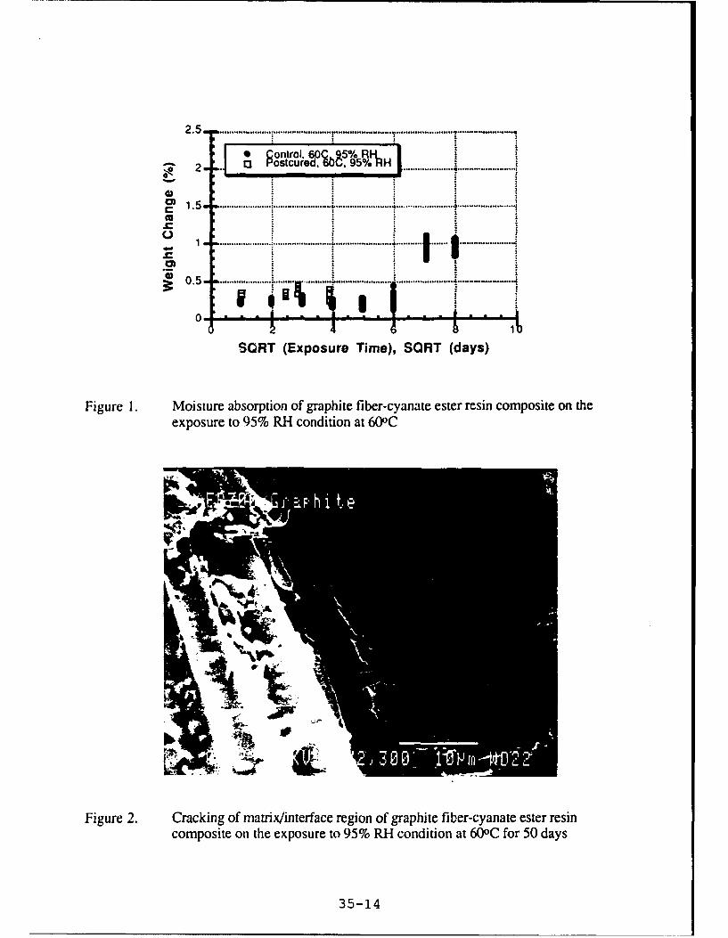
2.5 . ....................... ......................... .. .............. ..... : ......................... ....... . . .....
I*C ntrol. 60 5%RI I2 torost ured. ~..95% H
I 1 -.5 ............ ................ i ..................... 95 R i ........................ 4 ..... .................
U 1. . .............. ........ ......................... ........................ . ............. ........ ... ................... -I01.5 ....................... .. ..... ....... o...... ....
4- I
SORT (Exposure Time), SORT (days)
Figure 1. Moisture absorption of graphite fiber-cyanate ester resin composite on theexposure to 95% RH condition at 600C
r
Figure 2. Cracking of matrix/interface region of graphite fiber-cyanate ester resincomposite on the exposure to 95% RH condition at 600C for 50 days
35-14

10 0 , ............ ................ ............... ................ ............... ................ :.............. . . . .
.- = 70..t62 + j6.96451og(x) k= 0.9;712980-y= 58.124 + ;4.938dIog(x) R= 0.857998 0 . ........... ............... .............. ...... r..tate
-- 0-Moisture Saturatioo60 .... .......s-s
S4 0 . ............ o............... ............... ... " ... . , : ............... ............... .... .......... "'
U) 40
Si ~ ~ i=:=-
m 20 .......................... "........• ............... • ....... ,......... .-"........ ....._...
180 1. ! 1 b6
Fatigue Life (cycles)
Figure 3. S-N curves of dry and wet (50 days, 95% RH, 600C) specimens ofgraphite fiber-cyanate ester resin composite; Semi-log scale.
1 0 0 .......................................................... .............. ............... ............... ..............
i.-State-2 i ", i . |- "Misture Saturationl
ccc
C1 y :71.671J x (4.'058632) R. 0.97254-- y 58.053 XA(-'0.0447-46) Ri 0.850N4
180 10 b4 I "b
Fatigue Life (cycles)
Figure 4. S-N curves of dry and wet (50 days, 95% RH, 600C) specimens ofgraphite fiber-cyanate ester resin composite; Log-log scale.
35-15

(a)
(b)
Piue . Te rcur ufae o rpht ibrcant etrrei omo<
Figupei.The (ra)cture srf mnant of mraphtixrincggtohe fiberscat evenr rsncmo ite ahighly-fibrillated region (dry specimen): (b) the remnants of matrix resinwith an appearance of being easily peeled (wvet specimen).
3 5- 16

cc 10 0 . ....................................... ........ ............ ...................... ..........................................
rL •8 0" ...... 1 .................... ... ............... i .................... ....................................
60 .... .. ................60 . .... ...............
S . .................. ................... . . ...... .....................
, 20 ... 1 J88 CycljC ( 0 ..................../c......................i-r- 1~ 1atc
Exposure Time (days)
Figure 6. The changes of in-plane shear strength of graphite fiber-cyanate ester resincomposites after static exposure vs cycling to 1500C (Not postcured)
0 204C 'Cyclic (10 min/cycle)mm
1 0 20 4 C Static1 5 0 .......... ....... ;................... o•o°,.oo,,o,•..... ....... ... .,..,.°............. =............ .o....... .
CU •
a) :
U ) 1 0 0 .................. .................... 0......................................... .................... . ............
"50 1. 5
Exposure Time (days)
Figure 7. The changes of in-plane shear strength of graphite fiber-cyanate ester resincomposites after static exposure vs cycling to 2040C (Postcured)
35-17

Figure 8. Fluorescent dye-enhanced optical micrograph for the graphite fiber-cyanateester resin composite specimen subjected to thermal cycling to 150 0C
35-18
A STUDY OF THE GROWTH OF YBa2 Cu3 O7 -6 THIN FILMS ON LaAIO 3
BY PULSED-LASER DEPOSITION
M. Grant Norton
Assistant Professor
Department of Mechanical and Materials Engineering
Washington State University
Pullman W A 99164-2920
Final Report for:
Summer Faculty Research Program
Wright Laboratory
Sponsored by:
Air Force Office of Scientific Research
Boiling Air Force Base, Washington D.C.
September 1993
36-1

A STUDY OF THE GROWTH OF YBaCu3 07.6 THIN FILMS ON LaAIO 3
BY PULSED-LASER DEPOSITION
M. Grant NortonAssistant Professor
Department of Mechanical and Materials EngineeringWashington State University
Abstract
The growth of YBa 2 Cu 3 O7T6 thin films on LaAIO 3 substrates has been studied. The films were formed
using the pulsed-laser deposition technique. This technique employs a high energy laser to ablate material from a
target, the ablated material is deposited onto a substrate where film nucleation and growth can occur. The
microstructure and superconducting properties of the films were determined as a function of film thickness. It was
found that the films were close to the stoichiometric (123) composition, however there was evidence, both in terms
of the the film's microstructure and properties, to suggest the formation of secondary phases. X-ray diffraction studies
on similar films indicated that they consisted predominantly of grains oriented with their c axis perpendicular to the
film-substrate interface. Examination of the surface topography of the films using atomic force microscopy also
suggested the presence of grains oriented with the c axis in the film-substrate interface plane. Particles were detected
on the surface of all the films and the frequency of these particles depended upon the position of the substrate during
film growth. Films grown on substrates located on the left hand side of the sample holder had fewer surface particles
than films grown on substrates mounted in the center and right hand side of the sample holder.
36-2

A STUDY OF THE GROWTH OF YBa2Cu30 7.6 THIN FILMS ON LaAIO 3
BY PULSED-LASER DEPOSITION
M. Grant Norton
Since the discovery in 1986 of high-temperature superconductivity in oxide ceramics [1] there has been
extensive research in this field. This research has been directed into a number of areas-the formulation of new
materials with increasing transition temperatures, fabrication of existing materials into various forms, and
investigation of possible device applications. Because of the low critical-current densities in bulk superconductors
and the difficulties in making high-Tc superconducting wires and single crystals, the use of thin films may represent
the first major commercial application of this technology.
Many thin film deposition techniques employ high substrate temperatures to obtain oriented crystalline
films. High-temperature deposition often imposes a major impediment to the use of these materials in thin film
form because; (a) deleterious interactions may occur between the film and the substrate, degrading or modifying the
properties of the film 121 and (b) low-temperature deposition may be required for compatibility with existing
technologies. Furthermore, high-temperature deposition of a number of superconducting materials is problematic
because they involve constituents with widely varying vapor pressures or high melting points. The control of
composition and crystal structure in such materials is difficult at practical source and substrate temperatures.
The major obstacle to low-temperature growth is the difficulty of obtaining the high surface mobility
required for the nucleation and growth of crystalline or epitaxial films at low substrate temperatures. This limitation
may be overcome by delivering the material to the substrate in unique chemical forms (e.g., clusters or reactive
species), in charged or highly excited states, and/or with appreciable kinetic energy. This objective may be
accomplished in many ways, but among them, pulsed-laser deposition (PLD) offers significant advantages.
PLD utilizes the material ablated from a target as the source of deposited material. The rate of material
removal from the target can be varied considerably, from isolated atomic and ionic species, to nanometer-sized
dusters, to macroscopic (> llpm) fragments (ejecta). In any given deposition or etching process, control of the
emission rate and distribution is of considerable importance. In the case of thin film synthesis, atomic/molecular
neutral and ionic species are most desirable. These vapor-phase products are transported and deposited onto a substrate
36-3

where, given sufficient kinetic energy, they find low-energy configurations. The enhanced kinetics provided by
energetic particles can be exploited to cause nucleation of the growth of epitaxial films at low substrate temperatures.
PLD has proven to be a very versatile technique for growing both oxide and non-oxide films largely due to
the availability of high-power excimer lasers [3]. The laser-target interaction produces a high-temperature plasma
consisting of high-velocity and electronically excited neutral atoms, molecules, tions, and electrons. The kinetic,
electronic, and chemical energies of each of these constituents play important roles in film growth. The advantages
of PLD include:
* epitaxial or crystalline growth at low substrate temperatures,
* congruent deposition of materials with complex stoichiometries,
* facile deposition of materials with high melting points, provided they strongly absorb thelaser power,
* ability to form metastable microstructures, due to the low substrate temperature and thenonequilibrium nature of the ablation process.
Thin films of YBa2Cu 3OT7- 6 (YBCO), which has been the most widely studied of the superconducting
oxides, have been deposited onto a number of different substrate materials, including single crystals of MgO [e.g.,
Ref. 41, SrTiO3 [e.g., Ref. 5], and LaAIO 3 [e.g., Ref. 61, and polycrystalline substrates of MgO [e.g., Ref. 71 and
yttria-stabilized zirconia [e.g., Ref. 81. The choice of substrate is mainly determined by two criteria: (a) the deposited
films should have the desired physical properties, which often means that a close lattice match between film and
substrate is required, and (b) the substrate should be suitable for device or technological applications, for example. it
should have a low or moderately low dielectric constant. The lattice parameters of some commonly used substrate
materials and their mismatch with YBCO are shown in Table I.
Table I. Lattice parameters and mismatch between YBCO and various substrate materials [9].
nMaterial Lattice Parameter (rnm) Lattice Mismatch (%)YBa 2Cu3 07 0.382 _
MgO 0.421 9.7SrTiO3 0.391 2.3LaAIO3 0.378 -1.1
36-4

From Table I it can be seen that LaAM0 3 is closely lattice matched with the basal plane of the YBCO and
thus provides a suitable substrate for the growth of oriented films. In this study, (001)-oriented single crystals of
LaAIO3, prepared by the Czochralski process [101, were used.
A number of different laser systems, operating over a range of different processing parameters, have been
successfully used to produce thin films of YBCO. Changes in the processing parameters do. however, affect the
microstructure and/or the morphology of the films and, in turn, their properties [e.g., Refs. 11-15]. Some of the
parameters which have been considered in the PLD process are listed in Table 11. These parameters have been
classified as primary, secondary, and tertiary to denote their role in the deposition process. The primary parameters
directly control the ablation process (e.g., to yield thermal or nonthermal equilibrium) and the nature of the ablated
species. Secondary parameters influence the growth and microstructure of the film, for example, whether the
resulting film is amorphous or crystalline and the orientation of epitaxial films. Tertiary parameters are other
variables in the deposition process which have not been well characterized as to their effect.
Table IL Effects of processing parameters on microstructure (15].
Category Parameters Effect on Process Possible Effects on_Microstructure
Primary Laser wavelength Thermal or non-thermal Retention of target stoichiometryLaser power density evaporation Formation of metastableLaser pulse repetition rate Ratio of neutral to ionic microstructures
species in the plasma ParticulatesKinetic energy of the ejectedspecies
Secondary Substrate temperature Surface mobility of the Establishment of epitaxyPartialpressurelambient ablated species Formation of metastable
microstructuresControl of crystal structure
Tertiary Substrate-target distance Film thickness Not knownIrradiated spot size Thickness distribution across
I substrate
In this present study, the growth and superconducting properties of YBCO films deposited on LaAMO3
substrates was examined as a function of film thickness. The film thickness was varied by changes in the deposition
time: the following deposition times were used; 5, 15,45, 125, and 250 seconds. All the film depositions reported
here were performed using the experimental conditions described in the following section. A systematic study on the
effects of variation of several of the processing parameters (e.g., pulse repetition rate and substrate temperature) on
the properties and microstructure of YBCO films was also conducted. The results of this latter study will be reported
elsewhere.
36-5

The YBCO films were formed by focusing a Lambda Physik LPX 305i excimer laser operating on KrF
(k = 248 un) on to a 1" diameter stoichiometric YBCO pellet. For film deposition, a laser energy of -440 mJ/pulse
was used, the pulse duration was 25 ns, and the pulse repetition rate was 20 Hz. The interaction of the laser beam
with the target surface produced a plume of ablated material which emanated perpendicular to the target surface. Prior
to film deposition, the YBCO target was polished using SiC paper and laser irradiated (pulse energy - 160 mJ) in the
deposition chamber for 3 minutes in an ambient of 160 mTorr of oxygen. This conditioning process was employed
prior to each deposition to ensure reproducibility in the target surface. During film growth the target was rotated at
10 rpm and the laser beam simultaneously rastered across the target surface to avoid preferential ablation.
For each film growth experiment, three single crystal LaAlO 3 substrates (5 x 5 x 0.5 mm) were mounted,
side-by-side, on a stainless steel plate using silver paint. After drying the silver paint (90 - 95*C, 15 min in air), the
stainless steel plate was mounted on the sample holder in the vacuum chamber. The distance between the YBCO
target and the substrates was 6.42 cm and there was an angle of 450 between the plane of the target surface and the
stainless steel plate. The substrates were heated by a tungsten filament lamp located just below the stainless steel
plate. The temperature of the substrates was controlled by a variable resistance power supply and monitored by a
thermocouple in contact with the stainless steel plate. The substrate temperature was measured by means of a two-
color infra-red pyrometer which could be focused on the surface of any of the substrates. The substrate temperature
(measured by the pyrometer) during deposition was -770°C. Film deposition was performed in a flowing oxygen
ambient (-160 mTorr). Following film deposition, the chamber was filled with oxygen, the heater was turned off and
the samples allowed to cool to room temperature at a pressure of -490 Togr. The experimental conditions mentioned
above represent the 'standard' set of deposition parameters used in this study. The only difference between films
grown in different runs was the deposition time. The following deposition times were used: 5, 15,45, 125, and 250
seconds. The reproducibility of the experimental conditions was determined by repeating several of the runs.
It should be noted that the three substrate positions on the stainless steel plate were not equivalent; there
was an asymmetry in the shape of the plume of ablated material. The plume was longer and narrower on the left hand
side and shorter and wider on the right hand side. This asymmetry appeared to be due to energy differences in the
profile of the incident laser beam. In the results discussed below, left, center and right correspond to the position of
the substrates as viewed in the direction of the incoming laser beam.
The superconducting properties of the films were determined using ac magnetic susceptibility
measurements. The background to, and the experimental details of, this nondestructive technique have been described
elsewhere [e.g., Refs. 16-181. The real part of the ac susceptibility (X') gives a rapid determination of the
36-6
superconducting transition temperature (Tc) of the film, whereas the imaginary part, related to the ac loss (X"),
supplies information on the volume behavior of the film which is dominated by coupling effects and so represents a
measure of the critical current density (Jj)- The coupling effects will be influenced by the presence of homophase and
heterophase boundaries in the film.
The surface topography of the films was determined using atomic force microscopy (AFM) (Digital
Instruments Nanoscope II) and scanning electron microscopy (SEM) (Hitachi S-900). The AFM was operated in the
contact mode, wherein a sharp tip attached to a bendable cantilever directly contacts the surface of the sample being
examined. The tip is then scanned laterally over the surface. The bending of the cantilever in response to surface
height variations is monitored by a detection system. AFM's can have resolution down to the atomic level however
in this study, because of the roughness of the films and the tip profile used, atomic resolution was not possible. The
Hitachi S-900 SEM had a field emission gun source and was operated at an accelerating voltage of 2kV. The samples
examined in the SEM were heated in a vacuum oven at 95°C for 12 hours prior to loading into the microscope to
avoid contamination of the specimen surface under the electron beam. Coating of the samples for SEM examination
was not necessary.
The thickness of the films and their average composition was measured with Rutherford backscattering
spectrometry (RBS) using 2 MeV Het ions. An incident angle of 35° was used with a scattering angle of 1700. The
RBS data were analyzed using the RUMP simulation program [19,201.
Results
RBS data obtained for the series of YBCO films is shown in Table III. The calculated thickness of the films
ranged from 17 to 455 nm. RBS measures the areal density of the film, i.e., the number of atoms per unit area, and
this value is converted to thickness by considering the density of the film. The uncertainty of RBS thickness
measurements depends on the accuracy of the ion stopping power tables in the simulation program (estimated to be
±20%) and on the estimated density of the film. For the purposes of the RBS simulation program, the films were
assumed to be 95% of theoretical density, or 6.06 g/cm3 . For films grown an substrates mounted in the center and
right hand side positions of the sample holder this estimate is probably close to the actual density of the film.
However, for films grown on substrates located on the left hand side of the holder the film density is less than 95%.
Examination of sample 406, in a cross-section geometry, using SEM gave a measured film thickness of 90 nm.
This value is approximately 15% larger than that determined by RBS on the same film, which would be consistent
with the observation that films deposited on substrates situated on the left hand side of the sample holder were less
dense than films deposited on substrates in the other two positions. Thus the density of films grown on substrates
36-7

placed on the left hand side of the sample holder, based on the differences in the two thickness measurements. is
-80% of the theoretical density.
The desired film stoichiometry is YBa2 Cu 3 0 7 , which in atomic percent is Y:Ba:Cu:O =
7.7:15.3:23.1:53.9. It can be seen from Table III that, in most cases, the films had compositions close to this
stoichiometry. The sensitivity of RBS to an element is proportional to the square of its atomic number. Thus, the
uncertainty in the cation composition measurements is small. However, for oxygen the uncertainty is much greater,
therefore precluding an absolute measurement of atomic percent. The overall uncertainty in the compositions of the
thicker films is estimated to be ±10%. In the thinnest films further uncertainty in the values of the cation ratio
exists because the atomic masses of Ba (from the film) and La (from the substrate) are similar, making them difficult
to distinguish.
Table m. RBS data obtained from YBCO thin films on LaAlO3.
Sample # Deposition Atomic Density Thickness (nm) Y Ba Cu 0
Time/Position (10 15 /cm2 )
413 5 sec /left
414 5 sec/center - 125 -17.4 3.4 17.2 13.6 65.8
415 5 sec/right
409 15 sec/left 200 27.8 7.0 15.1 20.1 57.8
410 15 sec/center 240 33.4 5.9 14.3 16.9 63.0
411 15 sec/right 125 17.4 5.9 14.3 16.9 63.0
406 45 sec /left 580 80.6 8.1 15.4 23.2 53.3
407 45 sec/center 450 62.6 8.5 14.2 24.5 52.8
408 45 sec /right 280 38.9 7.0 13.6 22.1 57.3
403 125 sec/left 1575 219 8.6 17.2 24.1 50.1
404 125 sec/center 1100 153 10.2 17.8 29.4 42.6
405 125 sec/right 900 125 8.1 15.3 24.3 52.3
416 250 sec/left 3050 424 8.9 16.1 21.0 54.0
417 250 sec/center 3270 455 8.0 14.6 24.1 53.3
418 250 sec/right 2150 299 8.6 17.2 29.0 45.2
36-8
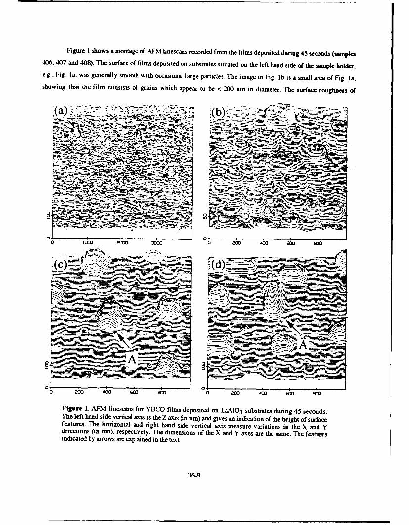
Figure 1 shows a montage of AFM linescans recorded from the films deposited during 45 seconds (samples406. 407 and 408). The surface of films deposited on substrates situated on the left hand side of the sample holder.e.g., Fig. Ia. was generally smooth with occasional large particles. The image in Fig. lb is a small area of Fig. Ia.showing that the film consists of grains which appear to be < 200 nrm in diameter. The surface roughness of
_ _ _ _ _
S000
Figure 1. AFM linescans for YBCO films deposited on LaAIO 3 substrates during 45 seconds.The left hand side vertical axis is the Z axis (in tim) and gives an indication of the height of surfacefeatures. The horizontal and right hand side vertical axis measure variations in the X and Ydirections (in rum), respectively. The dimensions of the X and Y axes are the same. The featuresindicated by arrows are explained in the text.
36-9

this area of the film was determined by AFIM to be - 2.8 nm. Films deposited on substrates located in the center
(Fig. Ic) and right hand side (Fig. ld) positions of the holder generally exhibited more surface features In Fig. Ic
some of these features are higher than 100 rin (indicated by the flat top of grain A). The exact shape of these
particles could not be determined by AFM due to the pyramidal profile of the tup. In Fig. Id it can be seen that some
of the surface features were elongated. e.g.. grain A, and these grains were found to be aligned in mutually
orthogonal directions. The shape of these grains is suggestive of YBCO where the c axis is 13 ing in the plane of the
film surface (a-axis oriented) [211. The underlying granular structure in all the films was determined by X-ray
diffraction to be predominantly c-axis oriented YBCO. Small peaks were observed which could be assigned to a-axis
oriented material.
The observations mentioned above, for the films deposited during 45 seconds, were consistent with AFM
data recorded from films grown during other deposition times. In particular, the number and shape of particles on the
surface of the films appears to be a function of the position of the substrate on the sample holder during deposition.
The surface of films deposited during 250 seconds on substrates located on the right hand side of the sample holder
was covered with particles, many of these particles having the elongated shape shown in Fig. Id. It is important to
note that, in general, the presence of these surtace features does not appear to be detrimental to the bulk
superconducting properties of the films.
The AFM data were qualitatively supported by SEM images recorded from films grown during 250 seconds.
Figures 2a and b, show secondary electron images (SEI) recorded from YBCO films deposited on substrates placed on
the left hand side (287) and right hand side (288) positions of the sample holder, respectively. It can be seen from
Fig. 2a that the film is not fully dense; large voids are clearly visible, some of which may penetrate to the film-
substrate interface. This observation is consistent with the films deposited on the left hand side of the sample holder
being only -80% of theoretical density. Slight differences in contrast are visible within the grains, these may be due
to compositional variations in the film. Film 288 shows a much denser microstructure, however small (20-30 nm
diameter) voids can be seen at grain intersections. Also visible in this image are several large particles on the film
surface. The size of thtse particles is consistent with some of the particles seen in AFM images recorded from the
same film. The origin of the white speckling in Fig. 2b is not known.
All the films showed superconducting properties although significant differences were observed in these
properties both as a function of film thickness and of substrate position. Figure 3 shows the temperature dependence
of the complex magnetic susceptibility with varying ac field (h) for specimens 406,407, and 408. The series of lines
represents varying applied ac fields; from 1 to 7 the fields are 0.025, 0.10, 0.25, 0.50, 1.0, 1.5, and 2.2 Oe,
respectively.
36-10

Figure 2. SHM images of laser deposited YBCO films on LaAIO 3 . The film shown in (a) wasdeposited on a substrate located on the left hand side of the sample holder (287), the film shown in(b) was deposited on a substrate located on the right hand side of the sample holder (288).
In film 406, two distinct superconducting transitions were detected, one at 71 K. the other at 64 K. The
transition temperatures of films dleposited on substrates located on the left hand side of the sample holder generally
were considerably less than the maxximtu Tc of 92 K. Single superconducting transitions were determined for films
407 and 408, at 87 K and 84 K, respectively. The lack of a distinct sccondary structure in thesc data implies that the
films are more uniform in superconducting properties over their entire area, although the shapes of the "C(F) curves
indicate the presence of unresolved distributions in the film parameters, especially in filn 408. The transition
temperatures deternuned for all the films grown in the center and right hand side of the holder varied slightly, but in
general these films were characterized by much higher Tc's than those obtained for films grown on substrates located
on the left hand side of the sample holder. lhe spreading of the X'(I') curves as a function of the ac field arises out of
the inability of the films to carr, the ciurrent required for full shielding of the fields and is thus inversely related to Jc
In the ideal situation the spreading of the curves would be a minimum.
36-11

(a) 406+ "
7
I I II I I 1 I o • l 6 • o l o l,
7
11
.| I I1 I I I I I , I I I I i 1 1 I a I
TEMPERATURE (X) TEMPERATURE (K)
Figure 3. Temperature dependence of the complex magnetic susceptibility with varying ac field.(a) real part, X'-. (b) imaginary part (loss). x".
36-12

The variation with temperature of the ac loss parameter, X", is shown in Fig. 3b for samples 406, 40(7. and
408. These curves portray the cyclic energy dissipation as the ac flux penetrates into the sample. The loss is
proportional to the superconducting volume which is penetrated by the field, and therefore such data provide a
sensitive measure of the material's overall properties and their distributions. The broadening and shift to lower
temperatures of the main loss peaks, as the ac field is increased are again characteristics of the weak-link intergranular
behavior which is prevalent in these ceramic superconducting materials [22). Thus, for the data shown in Fig. 3, the
critical current density of film 407 would be expected to be the highest if all the films were of the same thickness.
Discussion
Based on the RBS data, no systematic trends in the composition of the YBCO films was observed, either in
terms of substrate position or film thickness. The uncertainty in the cation composition of the thinner films
precludes any reasonable discussion on the apparent Y and Cu depletion in these films. One of the stated advantages
of the PLD process has been that the stoichiometry of the target can be reproduced in the deposited film. This
statement is true but only undee, certain deposition conditions. For arbitrary deposition conditions it has been shown
that the stoichiometry of YBCO films may be different from the target and this difference appears to have a spatial
effect [23241. Because the growth of YBCO thin films using PLD is typically carried out under non-equilibrium
conditions most films contain a high density of defects [e.g., Ref. 25]. These defects are often stacking faults
associated with the addition of extra layers in the YBCO lattice. For example, double CuO layers (YBa2 Cu4O8
structure) appear as isolated stacking defects within a matrix of a material that is predominantly found to have a
single CuO layer (YBa 2 Cu30 7 ) structure [26]. Examples of different layered defects have been observed by other
groups [e.g., Refs. 27-29].
Although no evidence for compositional defects could be obtained from the RBS data, the presence of
different phases in some of the YBCO films deposited in this study is suggested by the ac magnetic susceptibility
data. Examination of Fig. 3a, shows clear evidence of two distinct superconducting transitions. A possible
explanation for this effect may be the presence of different phases in the film, each possessing a different Tc. Small
deviations in measured Tc from the maximum value of 92 K, can often be accounted for by insufficient oxygen in
the crystal structure. Ex situ annealing studies at low temperature (- 5000 C) of similar YBCO films at Wright
Laboratory has shown to result in an increase in the Tc of the film.
The contrast variations observed in the SEM images, shown in Fig. 2a. also suggest the presence of
distinct phases in these films [301. Unfortunately, the SEM used in this study was not equipped with a backscattered
electron detector. Backscattered electron imaging (BEI) has a much higher sensitivity to compositional variations in a
36-13
sample. Characterization of the films using transmission electron microscopy ([EM) is in progress and it is hoped
that these studies will provide further information on the microstructure of these materials.
Ex situ annealing of these films at much higher temperatures (900 - 9200C 1311). where the YBa2Cu3 07
stoichiometry is favored, should lead to single superconducting transitions in the X'(T) curves if the observed
behavior is due to different YBCO stoichiometries. In the low temperature annealing studies it was noted that, in
general. annealing resulted in the lowering of the Jc of the film, this may be due to diffusion of the excess cations
toward the surface and grain boundaries of the film as was noted by Fendorf et al (25]. in a study of the kinetic
evolution of microstructures during 124 and 247 transformations to 123.
AFM studies revealed significant differences in the morphology of the various YBCO films. These
differences were more apparent as a function of substrate position during film growth, than as a function of film
thickness. Films deposited on substrates located at the left hand side of the sample holder bad a granular morphology
with significant intergranular porosity. The depth of these pores could not be resolved in the AFM, but from the
SEM results shown in Fig. 2a they may go to the substrate surface. These films have fewer surface particles than
films grown on substrates located in the other positions of the sample holder. In all films occasional large, - 1 pum
in diameter, particles were observed. It is proposed that these particles, which occur at random on the film surface,
arise due to melting of the target. In SEM examination they appear spherical indicating melting and often have a
composition close to stoichiometric YBCO [e.g., Refs. 32,33]. Particles having a similar appearance are often
observed to form during the ablation of other materials, for example during rapid ablation of sodium trisilicate glass
at high fluences, spark-like incandescent particles can be seen leaving the glass surface. These are small, molten
glass particles created by hydrodynamic sputtering [34). In the case of glass, repeated transient heating leads to the
formation of rolling surface asperities which grow from pulse-to-pulse until the tips fly off the target surface.
Films deposited on substrates located in the center of the substrate holder show a number of different
features; small (20 - 50 nm) grains, larger (- 0.2 lam) equiaxed grains, and elongated grains where one edge is
- 0.2 jam and the other - 0.4 .Am. In some of the samples examined several of the small grains had an acicular
appearance where others were equiaxed because these particles are so small it is not yet clear if they are the same or
different. The large elongated grains were found to be aligned in mutually orthogonal directions. AFM provides no
chemical information about the particles although similar features have been observed in other studies of YBCO
films where chemical analysis has been performed [33-351. Very small cube shaped particles, observed in YBCO
films on SrTiO3 substrates formed by dc hollow cathode magnetron sputtering by Catana et al [35], have been
identified as Y2 0 3 . Chang et al [33] observed very small surface particles (< 0.1 pm) which they suggested were
incipient nuclei for a-axis oriented YBCO particles. The larger elongated particles have a shape suggestive of a-axis
36-14

oriented YBCO grains [21]. although, as typified by grain A in Fig. Id, they have a terraced surface which is not so
usual. Again, similar particles were observed by Catana et al [35] and identified as either Y20 3 or CuYO2
precipitates. Further characterization of these features is obviously necessary.
Films deposited on the right hand side of the sample holder show the highest frequency of surface particles.
These surface particles are mainly the large elongated grains and the larger equiaxed grains, although the smaller
features are also seen. If these elongated grains are due to a-axis oriented YBCO then this type of surface morphology
would be consistent with that seen in TEM studies of YBCO films grown on (001) oriented LaAIO3 substrates [e.g..
Refs. 3637]. Examination of specimens prepared in a cross-section geometry by TEM show that the YBCO layer
next to the substrate surface is completely c-axis oriented but above a film thickness of about 400 nm. nucleation of
a-axis oriented grains occurs. Hence the film close to the substrate surface is c-axis oriented and at larger thicknesses
a-axis oriented.
Another feature of interest seen in both the SEM and AFM images of films deposited on substrates located
on the right hand side of the sample holder is the spherical voids. These voids are 20 - 30 nm in diameter and appear
similar to voids observed in YBCO films grown on MgO [38]. TEM investigations have revealed incipient
dislocations to be associated with these voids [38,39]. If the void was to be filled a dislocation would have to be
formed and this may be energetically unfavorable 140).
The morphology of laser ablated YBCO films on SrTiO3 has been examined as a function of substrate
temperature (Ts) and oxygen pressure (p02) by Borck et al [41]. They found that the morphology of the films could
be distinguished into distinct zones, associated with specific deposition parameters. The results of their study agreed
with the model proposed by Thornton [421. where the appearance of the zones are described below:
Zone I: The low adatom diffusion leads to a film consisting of tapered crystallites which are poorly
bonded and have a rough surface. Surface recrystallization may cause the grains to be
single crystals which diameter increases with p02 and Ts.
Zone T: The films consist of densely packed columner grains separated by dense grain boundaries.
The adatom diffusion is sufficient to overcome substrate and nucleation roughness and
leads to smooth surfaces.
Zone 11: Surface faceting causes 'open' boundaries between the grains because of the great adatom
diffusion. The grain size increases with Ts.
Zone III: Large substrate temperatures lead to large grains produced due to volume crystallization.
36-15

Thornton's model [421 deals only with pressure and temperature changes. Brock et al [411 showed that
variations in the laser energy density (E) could produce changes in the film morphology. In the region where
E - I - 3 J1cm 2 the films exhibited outgrowths which became larger and more numerous as E was decreased. Smooth
films were obtained at E - 3 - 5 J/cm 2 and films ablated at E > 5 J/cm 2 were of significant roughness. This cited
study is interesting and may provide a correlation to our studies where variation of several of the deposition
parameters has been performed.
Many recent studies of the growth of YBCO films using scanning probe microscopy have shown the
presence of a high density of screw dislocations (e.g.. Refs. 43-46]. The screw dislocation mediated growth
mechanism involves the addition of adatoms to the surface step which is always present along the edge of each spiral
shaped growth terrace emanating from a screw dislocation [e.g., Refs. 47,481. In the AFM images recorded in this
study there was strong evidence to suggest that this growth mechanism was occurring in these laser ablated YBCO
films on LaAIO3 substrates, however, we did not observe the individual steps. Thomson et al [49] qhowed that in
samples imaged by STM where the individual unit cell high steps associated with the screw dislocation mediated
growth could be easily seen they were not resolved in the AFM images, which showed only the broad outlines of the
gross surface structure.
MGN acknowledges numerous interactions with colleagues at Wright Laboratory, especially Dr. Rand Biggers,
Dr. Iman Maartense, Dr. Patrick Hemenger, and Timothy Peterson. Technical support and assistance from David
Dempsey, Jeff Brown, and John Woodhouse is greatly appreciated. The RBS analysis was performed at the Army
Research Laboratory in Watertown MA by Dr. J. Derek Demaree.
1. J.G. Bednorz and K.A. MOller, Z. Phys. B 64, 189 (1986)
2. X.D. Wu, A. Inam, T. Venkatesan, C.C. Chang, E.W. Chase, P. Barboux, J.M. Tarascon, and B. Wilkens,
Appl. Phys. Lett. 52, 754 (1988)
3. See, for example, papers in: Laser Ablation for Materials Synthesis, edited by D.C. Paine and J.C.
Bravman, Mater. Res. Soc. Symp. Proc. 191 (1990)
4. S.E. Russek, B.H. Moeckly, R.A. Buhrman, J.T. McWhirter, A.J. Sievers, M.G. Norton, L.A. Tietz,
C.B. Carter, in: fiEh Temoerature Sunerconductors: Fundamental Properties and Novel Materials
Processing, edited by J. Narayan, C.W. Chu, L.F. Schneemeyer, D.K. Christen, Mater. Res. Soc. Symp.
Proc. 169, 455 (1990)
5. G. Koren, A. Gupta, E.A. Giess, A. Sergmuller, and R.B. Laibowitz, Appl. Phys. Lett. 54, 1054 (1989)
36-16

6. R.W. Simon, C.E. Platt, A.E. Lee, G.S. Lee, K.P. Daly, M.S. Wire, J.A. Luine, and M. Urbanik, Appl.
Phys. Lett. 53, 2677 (1988)
7. B.H. Moeckly, S.E. Russek, D.K. Lathrop, R.A. Buhrman, M.G. Norton, and C.B. Carter, Appl. Phys.
Lett. 57, 2951 (1990)
8. D.P. Norton, D.H. Lowndes, J.D. Budai, D.K. Christen, E.C. Jones, K.W. Lay, J.E. Tkaczyk, Appl.
Phys. Lett. 57, 1164 (1990)
9 M.G. Norton and C.B. Carter, in: Laser Ablation for Materials Synthesis, edited by D.C. Paine and J.C.
Bravman, Mater. Res. Soc. Symp. Proc. 191, 165 (1990)
10. G.W. Berkstresser, A.J. Valentino, and C.D. Brandle, J. Cryst. Growth 109,467 (1991)
11. M.G. Norton and C.B. Carter, Physica C 172, 47 (1990)
12. G. Koren, A. Gupta, R.J. Baseman, M.I. Lutwyche, and R.B. Laibowitz, Appl. Phys. Lett. 55, 2450
(1989)
13. M. Balooch, D.R. Olander, and R.E. Russo, Appl. Phys. Lett. 55, 197 (1989)
14. R.E. Muenchausen, K.M. Hubbard, S. Foltyn, R.C. Estler, and N.S. Nogar. Appl. Phys. Lett. 56, 578
(1990)
15. M.G. Norton and C.B. Carter, Physica C 182, 30 (1991)
16. I. Maartense, J. Appl. Phys. 53, 2466 (1982)
17. D.W. Chung, I. Maartense, T.L. Peterson, and P.M. Hemenger, J. Appl. Phys. 68,3772 (1990)
18. A.K. Sarkar, B. Kumar, 1. Maartense, and T.L. Peterson, J. Appl. Phys. 65, 2392 (1989)
19. L.R. Doolittle, Nuci. Instrum. Meth. B 9, 334 (1985)
20. L.R. Doolittle, ibid, 15, 227 (1986)
21. M.G. Norton, S. McKernan, and C.B. Carter, Philos. Mag. Lett. 62, 77 (1990)
22. 1. Maartense, A.K. Sarkar, and G. Kozlowski, Physica C 181,25 (1991)
23. T. Venkatesan, X.D. Wu, A. Inam, and J.B. Wachtman, Appl. Phys. Lett. 52, 1193 (1988)
24. M.C. Foote, B.B. Jones, B.D. Hunt, J.B. Bamer, R.P. Vasquez, and L.J. Bajuk, Physica C 201, 176
(1992)
25. M. Fendorf, M.E. Tidjani, C.P. Burmester, L.T. Wille, and R. Gronsky, in: High Tc Superconductor Thin
Films, edited by L. Correra, Elsevier Science Publishers, Amsterdam (1992) p. 771
26. H.W. Zandbergen, R. Gronsky, and G. Thomas, Phys. Stat. Sol. A 105, 207 (1988)
27. R. Ramesh, D.M. Hwang, T. Venkatesan, T.S. Ravi, L. Nazar, A. Inam, X.D. Wu, B. Dutta, G. Thomas,
A.F. Marshall, and T.H. Geballe, Science 247, 57 (1989)
28. T. Krekels, G. Van Tendeloo, S. Amelinckx, J. Karpinski, S. Rusiecki, E. Kaldis, and E. Jilek, Physica C
178, 383 (1991)
29. Y.X. Guo, R. Hoier, T. Graf, and 0. Fischer, Physica C 199, 435 (1992)
36-17

30. D.K. Bowen and CR. Hall, Microscopy of Matenals, The MacMillan Press, London (1975)
31. N.-L. Wu. H.-D. Yu, Y.D. Yao. and E. Ruckenstein, Appl. Phys. Lett. 63,687 (1993)
32. M.G. Norton, L.A. Tietz, S.R. Summerfelt. and C.B. Carter, Appl. Phys. Lett. 55, 2348 (1989)
33. C.C. Chang, X.D. Wu, R. Ramesh, XX. Xi. T.S. Ravi, T. Venkatesan, D.M. Hwang, R.E.
Muenchausen, S. Foltyn, and N.S. Nogar, Appi. Phys. Lett. 57, 1814 (1990)
34. P.A. Eschbach, J.T. Dickinson, S.C. Langford, and L.R. Pederson, J. Vac. Sci. Technol. A 7, 2943 (1989)
35. A. Catana, J.G. Bednorz, Ch. Gerber, J. Mannhart, and D.G. Schlom, Appi. Phys. Lett. 63, 553 (1993)
36. C.W. Nieh, L. Anthony, J.Y. Josefowicz, and F.G. Krajenbrink, Appl. Phys. Lett. 56, 2138 (1990)
37. S.N. Basu, A.H. Carim, and T.E. Mitchell. J. Mater. Res. 6, 1823 (1991)
38. M.G. Norton and C.B. Carter, J. Cryst. Growth 110,641 (1991)
39. M.G. Norton and C.B. Carter, J. Mater. Sci. (1993 submitted for publication)
40. F.R.N. Nabarro, Theory of Crystal Dislocations, Dover, New York (1987)
41. J. Borck, S. Linzen, K. Zach, and P. Seidel, Physica C 213, 145 (1993)
42. J.A. Thornton, J. Vac. Sci. Technol. 12, 830 (1975)
43. Ch. Gerber, D. Anselmetti, J.G. Bednorz, J. Mannhart, and D.G. Schlom, Nature 350, 279 (1991)
44. M. Hawley, I.D. Raistrick, J.G. Beery, and R.J. Houlton, Science 251, 1587 (1991)
45. D.G. Schiom, D. Anselmetti, J.G. Bednorz. R.F. Broom, A. Catana, T. Frey, Ch. Gerber, H.-J.
Guntherodt, H.P. Lang, and J. Mannhart, Z. Phys. B 86, 163 (1992)
46. S.J. Pennycook, M.F. Chisholm, D.E. Jesson, R. Feenstra, S. Zhu, X.Y. Zheng, and D.J. Lowndes,
Physica C 202, 1 (1992)
47. F.C. Frank, Disc. Farad. Soc. 5, 48 (1949)
48. W.K. Burton, N. Cabrera, F.C. Frank, Philos. Trans. R. Soc. London Ser. A 243, 299 (1951)
49. R.E. Thomson, J. Moreland, N. Missert, D.A. Rudman, S.C. Sanders, and B.F. Cole, Appl. Phys. Lett.
63, 614 (1993)
36-18

GROUND AND EXCITED STATE PROPERTIES OF
LINEAR POLY(PHENYL) DI-METHYLENE
R.G. Petschek
Department of Physics, Case Western Reserve University, Cleveland, OH 44106-7079
Final report for the summer faculty research program
Polymer Branch, Materials Laboratory, Wright Laboratories, Wright- Patterson AFB
Sponsored by the Air Force Office of Scientific Research Boiling AFB
Wright Patterson Air Force Base ML/BP
September 30, 1993
37-1

GROUND AND EXCITED STATE PROPERTIES OF
LINEAR POLY(PHENYL) DI-METHYLENE
R.G. Petschek
Department of Physics, Case Western Reserve University, Cleveland, OH 44106-7079
Abstract
This paper presents ab initio (631G*) calculations for the properties of aw
n(para)phenyl-dimethylenes with n = 1,2,3. These molecules have two potential
radical centers separated by aromatic spacers and potentially have a variety of forms,
including the paired electron quinodial form, a singlet or triplet biradical form and
a pseudo-Jahn-Teller distorted form in with a spontaneous symmetry breaking and
opposite charges on the potential radical centers. The former quinoidal structure is
favored by electron pairing and charge separation rules, the others by resonance in
the aromatic rings. I find that for n = 1 this molecule is quinoidal and for n = 2,3
the molecule constrained to a D2h geometry is a singlet biradical and that the radical
wavefunctions are largely confined to the potential radical centers. More extensive
calculations in non-D 2h geometries have been done for the n = 2. The likely con-
sequences for polymers which consist of such potential radical centers connected by
aromatic segments and of polymers containing such radical centers are discussed.
37-2

GROUND AND EXCITED STATE PROPERTIES OF
LINEAR POLY(PHENYL) DI-METHYLENE
Rolfe G. Petschek
I. INTRODUCTION
The determination of the quinoidal, aromatic or other nature of molecules con-
taining two or more potential radical centers is of interest for a variety of reasons.
Small molecules with this property have been of interest for many years and have
properties distinctly different from those of molecules not containing such radical
centers [1]. Polymers have been proposed to have better conductivity properties
when in the quinoidal form. However the quinoidal form generally has a higher en-
ergy than the aromatic form. Thus the extent to which potential radical centers can
induce or facilitate the adoption of a quinoidal structure in such polymers is of in-
terest. As the aromatic structure generally has lower energy long enough potentially
aromatic segments separating potential radical centers are expected to result in one
of the aromatic forms considered below. If the repulsive interactions between the
electrons dominate then I expect a singlet or triplet biradical in which two electrons
are not paired but are (one each) on the potential radical centers[l]. If there is an
effective attractive interaction or electron pairing dominates a charge separated state
is expected.
Additionally molecules of this nature are also of interest as it should be possible
to make polymers - "polyradicals" - whose electronic states consist to large extent of
unpaired, radical electrons separated by aromatic or other portions. Such polymers
are likely have interesting new electronic and optical behaviors. Poly-radicals may
have a variety of states. These include the "dimerized" state, alternating quinodial
and aromatic rings, as in the pernigranuline form of poly(aniline), a charge density
wave form in which the potential radicals have different charges; a conducting form in
which the radicals are mobile, various forms related to ground states of the Hubbard
model, including conducting, insulating, Nedl antiferromagnetic, and other states.
37-3

These electronic states, particularly those for the Hubbard model, involve states with
appreciable dynamic electronic correleation which are still a matter of research even
in simple model systems. Rather than attempting to address this problem I have
done calculations on small monomers and polymer segments to understand what part
of the potentially large parameter space a particular molecular structure is in. In
order to do so I have calculated both the ground and excited state properties as the
excited state properties as the excited state properties give indications of the nature
of the the motion of electrons from one radical center to the next.
I find that the phenyl (n = 1) is quinoidal and that the biphenyl (n=2) and
triphenyl (n = 3) are singlet biradicals, with rather low lying triplet excitations and
rather higher lying singlet excited states. On this basis I expect that the polymers
consisting of such molecules connected through the methylenes will be dimerized for
the phenyl and semiconducting probably antiferromagnets for the bi and tri phenyls.
All calculations were done using the GAMESS quantum chemistry package[5].
This paper is organized as follows. In the next section I discuss the various
potential states of the molecules under consideration, and in the third section the
give simple mathematical models and discuss their generalization to related polymers.
I also discuss generally the calculational techniques used for the computation. The
fourth section gives computational details. Finally our results and their potential
importance to various polymeric systems are discussed.
II. POTENTIAL MOLECULAR STATES
I discuss at a simple heuristic level the possible ground and excited states of the
molecules under consideration and give a simple hamiltonian in terms of which one
might expect to understand the behavior of small molecules and to extrapolate their
behavior to polymers. The generalization of such a hamiltonian to the electronic
properties of polymers is presented.
An a, wn-para-phenyl-dimethylene can have a number of possible ground states.
The simplest is the quinoidal Lewis structure in which all electrons are paired and
37-4

is naively expected to give a reasonable approximation to the structure of such
molecules. However it is important to note that in this structure we have elimi-
nated the resonance stablization associated with (each of) the aromatic rings. It
is therefore expected that for sufficiently large n another class of Lewis structures
should predominate, in which there can be resonance stablization of the aromatic
rings. There are three simple possibilities. First there can be unpaired electrons on
(or near) the potential radical center. As these radicals can be either in a singlet or
a triplet state this is two separate possibilities. Secondly there can be a pair of elec-
trons on (or near) a single potential radical center and a missing electron on (or near)
the other potential radical center, resulting in the broken symmetry charge separated
state. As the phenyl rings are aromatic these structures are resonance stablized.
In our initial calculations all these molecules were constrained to have D2h sym-
metry in the symmetric state and correspondingly would have C2', symmetry in the
charge separated state. This is an approximation to the actual situation for the
biphenyl which is expected to have a twist between the two phenyl rings and D2 sym-
metry. The symmetry expected from a complete minimization of n = 3 is not clear -
if the two rings twist equally and in the same direction the symmetry would be D 2,
if the rings twist in opposite directions the symmetry would be C2 . Such twists can
be suppressed in actual molecules without seriously altering the electronic properties
by connecting the two phenyl rings to earh other e.g. as in flourene. Thus these
D2h results are interesting in the abstract. However it is important to remark that
in the triplet and excited states of these molecules there may be rather large twists
so that the excited electrons can avoid each other, making our D2h approximation a
more serious approximation. I confirmed this possibility for the biphenyl but have
not done so for the triphenyl.
In the non-quinodial states the inter-phenyl bonds have more single bond charac-
ter and in consequence are expected to be more easily twisted and, by Le Chitlier's
principle, favored by the twisted structure which results from the hydrogen-hydrogen
37-5

repulsion. Thus constraining n = 2,3 to the D2h geometry if anything decreases the
biradical character. However it is likely to increase the triplet energy relative to the
biradical energy. I have verified this for the biphenyl by doing the singlet biradical
calculation in the general D2 geometry and also the D2d (perpendicular rings) and
neighboring triplet biradicals.
In order to understand and explore the possible aromatic states we have consid-
ered the simplest calculational techniques which will incorporate their major features.
The likely effects of additional terms in the calculation are discussed and to some
extent calculated. The quinoidal structure and charge separated structures consist
entirely of paired electrons and in consequence can be studied to first approximation
using a restricted Hartree Fock (RHF) calculational technique. These states can (po-
tentially) be found separately by first calculating the state of the system insisting that
the system have the full D2h symmetry and then relaxing this symmetry constraint.
In practice this was done by doing a full geometry relaxation with an RHF calculation
of the wavefunction. The symmetry of the wavefunction was then reduced to C, (no
symmetry) which allows for the distortion of the wave-function into the suggested
charge separated state (and others as well). An identical calculation was done in
the TCSCF geometry and approximation discussed below. No attempt was made to
explore the possibility that such states can exist only in non-symmetric geometries.
In practise I found neither such states found nor any indication thereof such as slow
convergence reflecting large susceptibilities or low lying excited states with the same
multiplicity as the ground states, which also indicate large susceptibilities and this
possibility was not pursued further. Results from the singlet excited state calculations
(and chemical intuition) suggest that the electronic repulsion is sufficiently large in
any case that such a state is unlikely to form.
The triplet biradical configuration has two unpaired electrons in a triplet config-
uration. These were studied also in the simpliest possible calculation, a multiplicity
3 restricted open shell Hartree Fock (ROHF) calculation. The singlet biradicals were
37-6

studied using a one pair generalized valence bond (GVB) calculation. This is some-
times called the two configuration self consistent field (TCSCF) calculation. It is a
multi-configurational-self-consistent field calculation with the two configurations con-
sisting of the RHF configuration and the configuration with a pair of electrons taken
from the RHF highest occupied molecular orbital (HOMO) and placed in the RHF
lowest unoccupied molecular orbital (LUMO). As is known and also as discussed be-
low, this is the simplest calculation which allows for a singlet biradical. Note that such
a calculation includes as a variational possibility the RHF or quinoidal calculation
and so taken literally this will always imply that the singlet biradical has a lower en-
ergy than the quinoid. In practise this is not a serious difficulty as calculationally the
phenyl is essentially quinoidal and the biphenyl and triphenyl are essentially biradi-
cal. The lowest lying singlet excited state (SES) of the system was calculated using a
no-pair GVB calculation. The SES calculation has not been completed sucessfully for
the triphenyl. Calculations were done of the equilibrium geometries of each of these
states and "vertical transitions", that is calculations of the energies and wavefunctions
for all states in the equilibrium geometries of all other states were also calculated.
III. MATHEMATICAL MODELS
In order to understand the importance of these states and also their importance to
potential poly-radicals consider the following simple two site - two electron (biradical)
model hamiltonian:
Hd=bx + (t+ax) clc 2 . - Ja•5 2 + U 1n(n 1 (1)
where ci, is the annihilation operator for electrons with spin s = - on site i = 1,2,
n= X 4.Is, 0i is the total electron spin on site i given by the appropriate products
of a Pauli matrices with creation and annihilation operators, x is a molecular dis-
placement with respect to which the energy states should be minimized. In principle
there are a number of such molecular displacements - one for each normal mode. In
this study I were interested only in the approximate magnitude of these displacive
37-7

terms and have considered together all displacements which retain the D 2t, geome-
try. For the biphenyl we separately considered the effects of non-D2h displacements.
The parameters in this hamiltonian are a molecular stiffness b, a hopping matrix el-
ement t, the dependence of the molecular energy on the molecular displacement a,
a site-site repulsion term u, which models Coulomb repulsion and is expected to be
positive, and the spin-spin interaction energy J, which is used to model the effect of
exchange interactions with other electrons in the system. This effective hamiltonian
is the simplest hamiltonian which contains the salient features of actual and potential
molecular biradicals.
Before discussing this hamiltonian note that this model can easily be generalized
to a polymer with N potential radical sites connected together resulting inN-I 1
Hp N-Ibx' + (t + ax,) Z cci+.1 - jai "6+ + u Z ni(ni - 1) (2)
where xi is now a molecular displacement between the Oh and i + 1" site and the
remaining variables have an identical interpretation to that which they have in the
two site model. This polymer model is quite difficult to solve and I will not attempt to
do so here. Note that it contains a variety of well-known models as special cases. Thus
the J = 0, u = 0 limit of the model is the Su-Schrieffer-Heeger (SSH) model [2], which
is commonly used as a model of poly(acetylene) and other poly(enes) and is known
to show the dimerized state which is characteristic of known conducting polymers.
The degree of dimerization is given, approximately by a 2t- 2b-1. This part of the
model would be well described by e.g. simple mean-field or RHF techniques. The
a = J = 0 limit is the well-known Hubbard model, which was one of the first models
of the conductor-insulator transition and is still intensively studied [4]. For large u
interactions are important and simple mean-field or RHF techniques are expected to
fail. This is the "biradical" limit and has been treated by a variety of techniques in
this simple model. For an actual quantum chemistry calculation multi-configurational
self-consistent field techniques are potentially required. The a = 0, u -. oo limit is
a model of one dimensional ferro- or anti-ferro- magnets. As the model has these
37-8

rather different behaviors in various different limits it is expected that it should be
possible to design and synthesize polymers which have behavior other than either the
"typical" SSH behavior or recently synthesized organic magnets. The computational
determination of biradical parameters given below is a step in this design process and
towards a deeper understanding of poly-radicals.
While the polymeric model is quite difficult to solve with precision (various lim-
its have been a topic of research for many years) the simple dime 'odel is easily
solved with the use of group theory. There are six micro-states fol lectrons on
two sites. They decompose into one triplet (three micro-states) which is odd under
exchange of the sites, a singlet which is odd under the exchange of the sites and two
singlets which axe even under this exchange. As the model is symmetric under spin
rotations and site exchange these subspaces are eigenspaces of the hamiltoi .an and
only a 2 x 2 hamiltonian needs to be diagonalized to find all the relevant states. In
molecular orbital language the triplet state is two electrons with the same spin, one
in the highest occupied RHF ground state molecular orbital (HOMO) and one in the
lowest unoccupied such molecular orbital (LUMO). The anti-symmetric singlet is a
symmetric pair of electrons with opposite spins with one in the HOMO and one in the
LUMO. Finally the two symmetric singlets are paired electrons with the two basis
states are 01, a pair of electrons in the LUMO, and 1,, a pair of electrons in the
HUMO. In the non-interacting u = 0 limit the energy eigenstates are precisely the
states given above. In the strongly repulsive u - oo limit the relevant symmetric sin-
glet states are ?t ± Oh, exhibiting post single determinant Hartree Fock correlations.
In this limit the low lying energy states consist essentially of one unpaired (radical)
electron on each site. When J = a = 0 these states, a symmetric singlet and a triplet
are degenerate to order 1/u so it is expected that the exchange interactions will make
the triplet the lowest energy state. The other two states, a antisymmetric singlet and
an excited symmetric singlet are, in the large u limit essentially the symmetric and
antisymmetric combinations of the state with two electrons on one of the sites and
37-9
no electrons on the other.
IV. COMPUTATIONAL DETAILS AND RESULTS
The molecules shown were initially assumed to be planar and to have D21 symme-
try. Starting from an initial geometry these molecules were first geometry optimized
using the RHF wave functions. Starting from the RHF geometry the geometry was
optimized using three other calculational techniques, one pair GVB or TCSCF, the
ROHF triplet and the GVB singlet first excited state. In all the calculations reported
herein the frontier orbitals, that is the highest occupied and lowest unoccupied molec-
ular orbitals (HOMO and LUMO) in the RHF, the singly occupied orbitals in the
triplet and excited state singlet, and the partially occupied orbitals in the one pair
GVB calculations were 7r orbitals and in all cases had the same symmetries.
The basis set used for this work was[5] 631G*. That this was adequate for ground
state properties was tested by comparing the electronic states at the 631G* configu-
ration with the electronic states for 321G*. These were quite similar. It is not expect
that 631G* will give adequate results for the energy difference between the ground
state and the singlet excited state, however.
The RHF HOMO was a B2, state, that is odd under reflection about the molec-
ular plane and even under all other reflections. The RHF LUMO was a B10 state,
that is odd under reflection about the molecular plane and odd under the reflection
which interchanges the two potential radical centers and even under the remaining
reflection. This symmetry property is "expected" and is consistent with the simple
model given above which has two molecular orbitals which differ in symmetry only
in that one is even and the other odd under interchange of the potential radical cen-
ters. The geometries of these states is given in table 1. The MCSCF parameters
are given in table 2. Note that the monophenyl seems to be rather well described as
a quinoidal structure and in particular the bonds which are expected to be double
bonds in the quinoidal structure have bond lengths typical of carbon-carbon double
bonds. In addition the modifications on doing the TCSCF calculation are rather
37-10

small, with the number of electrons in the HOMO small. Finally the geometries and
energies of the singlet and triplet are quite different. I conclude that this system is
well described by the quinoidal structure. In the two systems with longer intervening
potentially aromatic sections, however, none of these conditions hold. In particular
the equilibrium geometries are very different (particularly for the triphenyl) from the
RHF, dimerized geometry, the bond lengths in the phenyl rings are typical of those
in aromatic rings in both the TCSCF and triplet states and the TCSCF and triplet
states have very similar energies and geometries. I conclude that the ground state of
the biphenyl is not quinoidal but essentially a singlet biradical and that the ground
state of the triphenyl is either a singlet or triplet biradical (we do not consider the
very small energy difference between these two states in the triphenyl definitive.)
However we note that the geometries of the ground and excited singlet states are in
all instances rather different. Also note that the frontier orbitals which are relevant
to the biradical calculation are strongly centered on the potential radical centers.
This strong centering on the biradical centers is consistent with the energy of the
singlet being lower. If two electrons (or other particles which repel each other) are in
spatially overlapping states then the correlation hole, resulting from the fact that two
like spin electrons can not be in the same location will result in a lower energy for the
triplet because the repulsive interactions are not as strong. However if the electrons
are in well separated states then the fact that in the singlet state the tails of the
wave-function can overlap for the singlet (but not the triplet) will lower somewhat
the kinetic energy in the singlet. I find the latter case. In consequence of this localiza-
tion it is expected that the addition of other phenyl rings (e.g. as in the Chichibudin
hydrocarbon (bi-triphenylmethylene)[1]) will not greatly alter the ground state and
low lying triplet properties of the molecule.
The energies of the electronic states which I have considered in the equilibrium
geometries of the electronic states considered are given in table 3. Examination of
the Mulliken population data shows an appreciable change in the HOMO and LUMO
37-11

wavefuntions between the ground and triplet and singlet excited states. Thus the
biphenyl is not expected that the simple model of section III will adequately de-
scribe the results for this system. In consequence detailed calculation of the biradical
parameters was not pursued.
For the biphenyl I have also examined geometries which are not D2 1. The mini-
mum energy for the triplet is expected where there is small overlap between the two
states in which the unpaired electrons reside. When the phenyl rings are perpen-
dicular to each other the molecule has a D2d geometry; the HOMO and LUMO are
degenerate; and, in an appropriate representation, reside largely on the two different
rings. I have verified that if the molecule is displaced slightly from this D2d geometry
to a D2 geometry then the energy of the triplet increases. I have also optimized the
TCSCF singlet relaxing the geometry constraints to D2 . However the final run for
the D 2 geometry is still incomplete, although the energy is clearly very close to final.
I note from the table that, in fact, the triplet and TCSCF singlet for this molecule
are very close, with consideration of non-planar configurations essential to computing
which of the states has the lower energy. The current calculation predicts that this
molecule will have a slightly lower energy in the singlet state, consistent with obser-
vations of the Chichibudin hydrocarbon which seems to have a lower energy in the
singlet by to have an appreciable (2%) population of the triplet at room temperature.
As the triplet has three times as many electronic states and twice as many symmetry
elements as the singlet biradical and the entropy is not expected to be appreciably
different. This suggests an energy difference of Tln(3/(2 x .02)) z 0.1eV, compared
with our result (for a somewhat different molecule in vacua) of 0.10eV. Consider-
ing the smallness of the difference and the differences in environment and molecular
structure this agreement is remarkable. It should be noted that the actual electronic
structure, charges etc. are very similar: however the geometric structure is somewhat
different. This geometric difference makes the likely changes from solvent effects not
inappreciable on this scale.
37-12
V. DISCUSSION OF POLYMERIC BEHAVIOR
Now consider the likely nature of polymers made from such molecules. I have
in mind polymers in which there are potential radical centers along the polymer
backbone consisting of a carbon atom bonded to a hydrogen and to two aromatic
segments which form the polymeric backbone. Such carbon radicals are known to
be quite stable. It is important to note that if the aromatic segments are phenyl
then steric considerations require that there be a significant twist between the rings
attached to each potential radical. As above this will tend to increase the tendency
for the formation of radicals as it will favor single bonds which are a larger fraction
of the wavefunction in the radical than the quinodal system.
I found that the phenyl was quinodal. As it is also known that the pernigranu-
line form of polyaniline is an alternating sequence of quinodal and aromatic rings it
is reasonable to expect that the carbon analog should be similar, despite the differ-
ences in electro-negativity of carbon and nitrogen I expect that the carbon analog of
pernigranuline polyaniline is also an alternating quinoidal-aromatic polymer. On the
other hand the biphenyl and triphenyl are essentially aromatic and I expect in con-
sequence that the corresponding polymers are also essentially aromatic. The effects
of polymerization on such a system is that the potential double bonds which imply
quinoidal structure can have a number of positions in the structure - most simply that
in a typical quinoidal Lewis structure only one of the two linkage groups connected
to a radical is expected to be quinoidal. As there are also allowed Lewis structures in
which the double bonds are on the other linkage group the double bond character is
expected to be reduced in the polymer relative to that in the monomer. Thus poly-
merization will tend to promote the aromatic configuration over the pernigranuline
configuration. This is easily confirmed by a simple band structure calculation.
In the simplest view of this aromatic state there is one unpaired electron on each
potential radical site. The actual situation, of course, is considerably more com-
plex. First of all the unpaired electrons are actually not completely localized on the
37-13
potential radical sites. Thus there will be some changes in relative energies on poly-
merization. Secondly and more importantly the quantum states which correspond to
the monomer excited states in which there is more than one electron on the potential
radical sites or the frontier electrons are in the aromatic bridge have to be considered
in extrapolating the monomer results to a polymer. However there is a large difference
in the energy I have calculated for the differences between the TCSCF and triplet
states and the singlet excited state. I do not expect that our basis set, which did not
contain diffuse functions, is adequate to calculating this difference accurately (and,
in fact, the observed transition energy for the monomer is too high). Nevertheless
given the very large difference in energy differences it seems reasonable to hypothesize
that the states in which there is essentially an unpaired electron on each potential
radical site predominate at low temperatures for ground state like properties. In
other words to good approximation the polymer can be viewed as a Hubbard model
in the insulating (more properly semiconducting) strong repulsion (u -. oo) state.
This is well approximated by isolated, unpaired electrons with a barrier to conductiv-
ity comparable to the singlet-ground-state to singlet excited state energy difference
(approximately 6eV in my likely inaccurate calculation). As discussed above this is
likely an over-estimate. Nevertheless these polymers are expected on this basis to be
poor conductors at ordinary temperatures.
As the energy maximum for the low energy triplet spin state is only 0.10eV
above the energy of the "best" TCSCF singlet state it is expected that at ordinary
temperatures the phenyl rings will rotate freely - primarily in the triplet state as the
barrier to rotation in the singlet state is much larger than that in the triplet state.
However as it is also the case that energy difference between the singlet and triplet
state is much lower when the rings are allowed to rotate relative to each other it
is expected that at temperatures less than .eV -, 1000K there will be appreciable
correlation between the spins that there will also be correlation between the spin state
and the relative angle of the rings so that e.g. the rotation of the rings should be
37-14

apparent in the EPR spectra.
The energy difference between the singlet and triplet is rather small and it is not
immediate from this calculation whether parallel or anti-parallel aligned spins will
dominate in the polymer. The D2d triplet, which I hypothesize is the lowest energy
triplet, has energy higher than the twisted D2 singlet. As this is consistent with
expectations from the physical reasoning presented for the biphenyl in section III, we
hypothesize that the singlet is the lowest energy state. However it is important to
remark that the energy differences are rather small and are also (as is apparent from
table 2) strongly related to the conformation of the polymer. I expect significant
changes when this monomer is polymerized and possibly more subtile differences for
"a calculation in which more dynamic electronic dynamic electronic correlation or
"a superior basis set is used. Moreover the argument in section III applies in the
D2h geometry and does not apply in the D2d geometry in which the two radical
wavefunctions have completely different (ir and o) character where they overlap and,
in fact, the triplet has the lower energy in this configuration. On balance however it
seems more likely that the anti-aligned or singlet configuration has a lower energy.
If this is the case the polymer would be well approximated by a semi-conducting
antiferromagnetic state. Such states have been extensively studied and will not be
discussed here. If, on the contrary, the aligned state is preferred (which seems on
balance less likely) the low temperature state will be a semi-conducting ferromagnetic
state.
The optical properties of this state are also of interest. I do not expect that they
will be those of a extreme electron-electron repulsion Hubbard model. In particular
the excited states of the dimer are not well approximated by two electrons on one of
the radical centers and no electrons on the other radical center - rather the excited
electronic state is spread out over the entire (oligo)phenyl spacer between the two
radical centers. For the the poly-radical model (Eq 2) to apply to biphenyl and longer
spacers it seems, from the calculations above that it must use the t/u --* 0 limit. This
37-15

model supposes that energy of a state depends to lowest order only on the total
number of potential radical sites containing zero, one and two electrons. The excited
state of the monomer which is, at least qualatively expected to describe the excited
states of the polymer does not have this character, rather one of the orbitals involved
is concentrated in the (oligo)phenyl spacer. This relaxation of the electronic state in
the biphenyl portion separating the two radical centers will require additional terms
reflecting this relaxation when unoccupied and doubly occupied states are adjacent.
In principle this can be studied, at least in part by also studying various excited
and charged states of this monomer, and by studying the excited states of larger
molecules (e.g. the three radical dimer). The Hubbard model would then have to be
extended to include (at least) two states on each site (or one in on the spacer), one
of which has low energy but large electron-electron repulsion and the other of which
has a higher energy but allows for excited states with energies less than that of the
singlet excited state in which the electronic energy is appreciably raised by electron-
electron repulsion. As this second state seems not to reside largely on the potential
radical center it is likely also to be significantly effected by the groups attached to this
center so that appreciable difference are expected between the biphenyl dimethylene
I have studied and more stable molecules such as the Chichibudin hydrocarbon or
the potential polymers. Similar comments apply to the high temperature states of
the polymer, in which there is expected to be appreciable occupation of the singlet
excited state. A study of these issues is beyond the scope of this paper.
Acknowledgements: Work supported by the AFSOR though Bolling AFB and the
polymer branch of Wright Laboratories, Wright Patterson AFB. Detailed conversa-
tions with and the technical assistance of Douglas Dudis (who suggested the problem
to me), A. Todd Yeates and Steve Trohalaki are gratefully acknowledged.
37-16

REFERENCES
[1] See e.g. A.W. Wheland "Advanced Organic Chemistry" John Wiley and Sons,
New York (1960) p 813ff.
[2] M.W.Schmidt, K.K.Baldridge, J.A.Boatz, J.H.Jensen, S.Koseki, M.S.Gordon,
K.A.Nguyen, T.L.Windus, S.T.Elbert QCPE Bulletin 10 52-54 (1990).
[3] See e.g. A.J. Heeger, S. Kivelson, J.R. Schrieffer and W.-P. Su, Rev. Mod. Phys.
60 781 (1988).
[4] J.T. Gammel, R.J. Donohue, A.R. Bishop, and R.I. Swanson Phys. Rev. B42
10566 (1990) and references therein.
37-17

TABLES
Table 1: gives the equilibrium energies and geometries of a, W n-(phenyl)dimethylenes
in various electronic states. The symbols RHF denote the (theoretically interesting)
Restricted Hartree Fock state, TCSCF is the two configuration self consistant field
(HOMO - LUMO multiconfigurational self consistent field) calculation, Trip is the
lowest lying triplet state and SES is the lowest lying singlet excited state. I was un-
able to find the equilibrium geometry for the triphenyl. Only the distances between
carbons directly bonded to each other are given. All distinct such distances are given,
with the numbering scheme shown in figure 1. Energies are given in Hartrees, dis-
tances in angstroms.
n State Energy Rm, R12 R23 R4 R41, R1 ,2, R213'
1 RHF D2h -307.23557 1.3301 1.4702 1.3277
1 TCSCF D2 h -307.56556 1.3462 1.4532 1.3366
1 Trip D2h -307.53311 1.4588 1.395 1.3822
1 SES D2h -307.34700 1.4363 1.3904 1.3602
2 RHF D2h -537.06502 1.3319 1.4637 1.3310 1.4682 1.3622
2 TCSCF D2h -537.07477 1.4362 1.3986 1.3768 1.4000 1.4874
2 Trip D2 h -537.07226 1.4473 1.3953 1.3799 1.3969 1.4967
2 SES D2h -536.92095 1.3676 1.4422 1.3541 1.4310 1.4358
2 TCSCF D2 -537.07833
2 Trip D2d -537.07428 1.4484 1.3970 1.3821 1.4970 1.3912
3 RHF D2h -766.58084 1.3325 1.4632 1.3319 1.4655 1.3663 1.4594 1.3355
3 TCSCF D2h -766.61942 1.4450 1.3962 1.3794 1.3973 1.4943 1.3946 1.3807
3 Trip D2h -766.61920 1.4457 1.3958 1.3795 1.3970 1.4948 1.3943 1.3808
37-18

Table 2: Gives the MCSCF coefficients and energy lowering for the TCSCF calcula-
tions of the D2h molecules considered in this paper.
Molecule Orbital 1 Orbital 2 Energy Lowering
phenyl 0.9756 -0.2192 -0.0198
biphenyl 0.7763 -0.6304 -0.1534
triphenyl 0.7256 -0.6881 -0.1977
37-19

Table 3: Transition energy (eV) from the of equilibrium geometries of a number of
electronic states to other electronic states. Labeling of states as in Table 2. The
equilibrium geometry for the SES triphenyl is unavailable.
3a: Phenyl:
Equlibrium Geometry TCSCF Trip SES
TCSCF 0.0 2.072 6.109
Trip -0.622 0.0 5.131
SES -5.830 -4.423 0.0
3b: biphenyl:
Equlibrium Geometiy TCSCF Trip SES
TCSCF 0.0 0.075 4.676
Trip -.062 0.0 4.737
SES - 7 -3.531 0.o
3c: triphenyl:
Equlibrium Geometry TCSCF Trip SES
TCSCF 0.0 0.009
Trip -.009 0.0 -
SES -4.920 -4.911 0.0
37-20

SEMICONDUCTOR COUPLED AMPLIFIERS FORELECTRO-OPTIC APPLICATIONS
M. J. PotasekResearch Professor
Department of Applied Physics
Columbia UniversityNew York, New York 10027
Final Report For:Summer Research Program
Wright-Patterson
Sponsored by:Air Force Office of Scientific Research
Boiling Air Force Base, Washington, D.C.
1993
38-1

SEMICONDUCTOR COUPLED AMPLIFIERS FORELECTRO-OPTIC APPLICATIONS
M. J. PotasekResearch Professor
Columbia University
Abstract
Nonlinear optical phenomena are of interest because of their wide ranging
applications. In particular I have investigated coupled semiconductor waveguides of
interest in electro-optic applications. Because of the available semiconductor
growth facilities in the area and their growing importance in research, particular
attention was paid to the Ill-V semiconductor multiple quantum well materials.
38-2

SEMICONDUCTOR COUPLED AMPLIFIERS FOR
ELECTRO-OPTIC APPLICATIONS
M. J. Potasek
Because of the prospects of integration of several components such as lasers,
detectors and modulators, semiconductors are advantageous for electro-optic
applications. Semiconductor waveguides are of interest for applications ranging
from communications to computing. Considerable research has focussed on the
quantum confined Stark effect. However because of the electron hole recombination
dynamics, devices based on this concept have been slow. An alternative is the use
of >.;,.upled semiconductor traveling-wave amplifiers. A single semiconductor
amp.ifier is fabricated like a semiconductor laser with the exception of reflecting
cleaved ends on the waveguide. While a simple semiconductor amplifier
is useful for amplification in integrated circuits, other complex features re-
quire more complicated structures. For information processing, a nonlinear
directional coupler (NLDC) is often used. The NLDC was devised for optically
activated switching between two output ports (1) . The switching is achieved by
38-3

using in a linear directional coupler an intensity-dependent factor for the refractive
index This locally alters the wave vector mismatch between the guides, so that the
effective energy transfer and coupling length can be adjusted by varying the input
power. Directional coupler switches with optical gain have previously been
investigated in the linear regime (2). Recently, electrically and optically controlled
partial switching of continuous wave light was observed in a twin-ridge Fabry-Perot
amplifier (3). Here I consider a coupled system with distributed gain arising from
.arrier injection by pumping current into twin stripe contacts. The active device is
composed of two coupled traveling wave semiconductor laser amplifiers. In this
system self-switching arises from self-phase modulation (SPM) associated with
optically induced saturation of the gain. A schematic is shown below.
2 1
In addition to the optical gain I also include nonlinear absorption (two-photon
absorption TPA) and waveguide dispersion.
Mf1ATERIALS
Materials of interest are the III-V semiconductors. In particular, materials such
as InGaAs are of value because their bandgap lies in the .8 to .9 um spectral
38-4
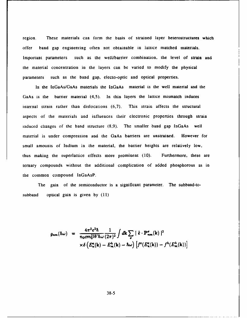
region. These materials can form the basis of strained layer heterostructures which
offer band gap engineering often not obtainable in lattice matched materials.
Important parameters such as the well/barrier combination, the level of strain and
the material concentration in the layers can be varied to modify the physical
parameters such as the band gap, electo-optic and optical properties.
In the InGaAs/GaAs materials the InGaAs material is the well material and the
GaAs is the barrier material (4,5). In thin layers the lattice mismatch induces
internal strain rather than dislocations (6.7). This strain affects the structural
aspects of the materials and influences their electronic properties through strain
induced changes of the band structure (8,9). The smaller band gap InGaAs well
material is under compression and the GaAs barriers are unstrained. However for
small amounts of Indium in the material, the barrier heights are relatively low,
thus making the superlattice effects more prominent (10). Furthermore, these are
ternary compounds without the additional complication of added phosphorous as in
the common compound InGaAsP.
The gain of the semiconductor is a significant parameter. The subband-to-
subband optical gain is given by (11)
4•r2e2h 1 Agn,(Iw) -- nocmoWhw (2•r) 2 ak & P:,,(k)12
x× (E:(k) - E"(k) - &w) [r(E.'(k)) - fh(EA(k))
38-5

where no is the index of refraction, c is the speed of light, W is the quantum well
width, hw is the photon energy and the f's are the distribuuon functions for
electrons in the conduction and valence bands. The total material gain is obtained
by summing over all subbands n,m and integrating against a Lorentzian
function (12),
g(E) = JdE'l g.,, (E') A(E - E').
The radiative current density is evaluated from the dipole transition rate (13) for
the quantum-confined carrier states,
S/ fd(A 4 e2no&, 1 12
X6 (E.:(k) - E•(k)- w) [fe(E:(k))][1 - f"(E•(k))]
At low concentrations the carriers obey Boltzmann statistics with the current being
proportional to the square of the injected carrier density n. But at higher carrier
densities the emission rate falls off from the n2 curve (11).
38-6

However the light only experiences optical gain in the well region, as a result it is
convenient to characterize the gain by a confinement factor given by
r = N-tW.
where N is the number of quantum wells used in the multiquantum well structure, W
is the width of each well and gamma is the optical confinement per unit width of
quantum well. A gain curve for InGaAs materials is shown below for 50 A wells for
various carrier injections (11).
6
4
-2
Z( -4
-6
-8-10 1.0
1.36 1.41 1.46 1.51 1.56 1.61
ENERGY (eV)
38-7

MODE EQUATIONS
I consider an active system composed of two parallel travelling-wave
semiconductor amplifiers with distributed gain arising from carrier injection by
pumping current into twin stripe contacts. The input beam is injected into channel 1
and the gain of each amplifier is adjusted by varying the pumping current I
(assumed the same for both waveguides) TFhe electromagnetic field is a superposition
of the modes of the isolated single-mode waveguides given as
2
E(x,Y.Z,t) Z- if, (x.y)A,(z,t)
exp {i(oz - WOI)) + c.c.I
where A is the slowly varying envelope of the electromagnetic field,
The linear coupling between the two modal amplitudes is provided by the evanescent
overlap of the two waveguide modes. The coupled equations are given by
I ± -L± A, = itcA, + .(l - cz)g 1(NI)A,
and
a- + -• A, = ioA, + 0I - ia)g2 (N,2 )A2.
38-8

where k is the linear coupling coefficient, alpha is the linewidth enhancement
factor, and the g's are the intensity gains (dependent on the carrier densities, N).
The linewidth enhancement factor is a constant independent of density. When k=O
the expressions reduce to an uncoupled semiconductor amplifier (14,15,16). For a one
coupling length device light will transfer from guide 1 to guide 2 without distortion
in the linear limit. When the optical pulse duration exceeds the intraband
relaxation time, the induced polarization can be eliminated and the field matter
interaction is given by a set of coupled field carrier rate equations. The carrier
densities for the semiconductors obeys the rate equations (14,16) given by
SN J g ,(N i)
8t q V Tr hc 1
where I is the injection current, q is the electron charge, and V is the cavity volume.
A linear dependence of the gain on the carrier density is used (17)
g,(N,) = ra(N, - NO) j = 1,2
where No is the transparency carrier density.
38-9
A cross section averaged gain relaxation equation is used since the waveguide
dimensions are smaller than the carrier diffusion length(19)
agi (g, - gjo) I 1,2at- - • E,,j jz
where Esat is the saturation energy, lo is the transparency current and go is the
small signal gain. A one coupling length device is considered so that at low input
intensities the light exits through the opposite waveguide. It is assumed that the
width of the pulse is much less than the carrier lifetime. As a result the amplifiers
are determined by the small signal gain and the linewidth enhancement factor.
Experimental values of the linewith enhancement factor is about 6 (18).
If the nonlinear absorption and dispersion are neglected, the uptical switching
performance is limited to 50% of the output energy (19).
NUMERICAL RESULTS
However dispersive and absorptive factors are important in semiconductor
devices. Therefore I incorporate these features and study their behavior using the
numerical beam propagation method (NBP). This numerical procedure uses the fast
Fourier transform to calculate the propagating field for a distance d/2 with
dispersion only and then one
38-10

multiplies the result by a nonlinear term representing the effect of the
nonlinearity over the whole segment d and again propagates the field for the
remaining distance with dispersion only.
Using the NBP method, I have investigated the behavior of the semiconductors.
The figure below shows the switching fraction as a function of input. The portion on
the left side corresponds to no dispersion (with less than 50% of the light switching)
whereas the right side includes the effects of dispersion ( with about 80% of the
light switching). The dispersion balances the pulse distortion caused by the
self phase modulation. This results in significant improvement in waveguide
performance and is an important consideration for future applications.
1.0 1 ,.0
10 zcO0.8 0.8 ,,/
0.060. cc
U.Z20.4-0.
0' -20n 0.2
- , ,
cn 0.2 0-2 /
0.0 02 6 0. 0.5 1.0 15 2.0
38-11

In semiconductors the effects of nonlinear absorption can cause distortion and loss.
Therefore I have also investigated this effect. The figure below shows the effects of
high power without the presence of the nonlinear absorption effects. On the left
side the light input to one waveguide is amplified and remains largely in that guide.
On the right side I show the opposite waveguide where little light has been
transferred. This figure shows good behavior for the semiconductor devices and
represents a significant result in this study.
-0 2
T IKE
0 u.
-4 -2 0 0, a
t31ME
38-12

Next I investigate the effects of the nonlinear absorption on the semiconductor. The
figure below shows the new behavior. On the left side the light is amplified and then
decays as the absorption takes place. On the right side the light is more of the light is
transmitted and the pulse shape is deteriorated. As a result one realizes that
wavelengths where the nonlinear absorption is minimized must be used.
10.
0.A
00.2
TI ME
TIME
38-13

SUJMMARY
I have investigated the behavior of semiconductor amplifiers for electrooptic
devices. Including more realistic physical parameters enables better device
characteristics. Future investigations involve the effects of the gain saturation, the
variation of the semiconductor alloy concentration, the number of quantum wells
and the well and barrier width. Waveguide fabrication can be performed at WPAFB
and semiconductor waveguides measured optically for waveguide loss and
performance.
38-14

Re fere nces1
1. S. M. Jensen, IEEE J. Quantum Electron. QE-18, 1580 (1982).
2. C. J. Setterlind and L. Thylen, IEEE J. Quantum Electron. QE-22, 595 (1986).
3. D.A. H. Mace, M. J. Adams, J. Sing, M.A. Fisher, I.D. Henning and W. J. Duncan,
Electron. Lett. 25, 987 (1989).
4. G. C. Osbourn, J. Vac. Sci. Tech. 21, 459 (1982).
5. S. T. Picraux, L.R. Dawson, G.C. Osbourne and W.K. Chu, Appl. Phys. Lett. 43,
930 (1983).
6. J. W. Matthews and A.E. Blakeslee, J. Cry. Growth, 27, 118 (1974).
7. G. Bastard, C. Delalande, Y. Guldner and P. Voisin, Advances in Electronics and
Electron Physics . P. W. Hawkes, ed, (Academic Press, NY, 1988).
8. F. H. Pollak and M. Cardona, Phy. Rev. 172, 816 91968).
9. J. Y. Marzin and J. M. Gerard, Superlattices and Microstructures, 5, 51 (1989).
10. K. J. Moore, G. Duggan, K. Woodbridge, and C. Roberts, Phys. Rev. B 41, 1090 (1990).
11. J. Loehr, Theoretical Studies of Pseudomorphic Quantum Well Optoelectronic
Devices, Technical Report N. SSEL-202, 1991.
12. G. D. Sanders and Y. C. Chang, Phys. Rev. B 35, 1300 (1987).
13. J. J. Sakurai, Advanced Ouantum Mechanics (Addison-Wesley, New York, 1967),.
14. N.A. Olsson and G.P. Agrawal, Appl. Phys. Lett. 55, 13 (1989).
15. G.P. Agrawal and N.A. Olsson, Opt. Lett. 14, 500 (1989).
16. G.P. Agrawal and N.A. Olsson, IEEE J. Quantum Electron., 25, 2297 (1989).
38-15

17. G.P. Agrawal and N.K. Dutta, Long Wavelength Semiconductor Lasers
(Van Nostrand, New York, 1986).
18. M. Osinski and J. Buus, IEEE J. Quant. Electron. QE-23, 9 (1988).
19. S. Trillo, S. Wabnitz, J. M. Soto-Crespo and E. M. Wright,IEEE J. Quantum Electron,
27, 410 (1991).
38-16

PUOTOCOOD-TCa VTr AMD RITATED STUDIE OF T IADDER POLUR
POL• ZEZaD ZOoPNTUROL1UE (33L)
Barney 3. Taylor
Visiting Assistant Professor
Departmant of Physics
Miami University - Hamilton
1601 Peck Blvd.
Hamilton, OH 45011
Final Report for:
Suir Faculty Research Program
Wright Laboratory
WL/MAP
Sponsored by:
Air Force Office of Scientific Research
Bolling Air Force Base, Washington, D.C.
September 1993
39 - I

PUOOzCOUDUC IVTT AND 3ZLAZ STUDIES OF TM LADDER POLUMPOL!UZJ=ZWC•=ASOZINTUOLZ (BBL)
Bazney Z. TaylorVisiting Assistant Professor
Depar~t t of PhysicsMiami University - Hamilton
Abstract
Polybenzimidazobenzophenanthroline(BBL) is a ladder polymer that offers
hope of electronically conducting polymers for future applications. Some of
the electro-optical properties of BBL have been investigated by
photoconductivity and related measurements. BBL exhibits a characteristic
spectrum, with a low-energy peak near 1.8 eV, and other stTucture. The
dependence of the BBL spectra upon chopping frequency of the pump beam and
applied electric field has been investigated. The PC response of BBL was
found to be dependent upon both; however, the chopping frequency dependence is
the more interesting. At low chopping frequencies (- 10 Hz), a single
exponential behavior was observed, while at higher chopping frequencies an
inverse power law response was noted.
Attempts were made to measure the carrier lifetime and mobility of BBL
by pulsed laser, time of flight experiments. Instrumental limitations caused
limited success, however, a photo-induced transient signal was observed that
is believed to be characteristic of BBL.
39 - 2
IBOTJLMDUCTXVIT! AND 1RATZD STUDZIS Of TM LADD. POLflR
POLY=ZUnDAZOUENZOlZinNTHOL (B5!)
Barney Z. Taylor
Introduction
Electrically conductive polymers offer great hope for the technology of
the future. Some of the improvements would be reduced aircraft weight and
greater latitude in manufacturing technology - such as vacuum forming of
conducting assemblies. The polymers of the future are under development
today. Ladder polymers have much greater thermal stability and mechanical
strength compared to conventional doped conducting polymers. 1 This document
reports on the research performed on the electro-optical characterization of
the conducting ladder polymer BBL (polybenzimidazobenzophenanthroline) by
meanE of photo-conductivity (PC) and related techniques. The research had
three major components: a study of trap lifetime in BBL by means of
photoconductivity measurements; a study of the effect of various electric
fields on the BBL PC spectrum; and a beginning investigation of the mobility
of the majority charge carriers in BBL by a time of flight technique. Each of
these components will be addressed separately. The experimental apparatus had
to be upgraded to allow the studies to be performed. A summary of the
enhancement to the experimental capability is in the Appendix.
WTLUA.rL AND DATA
The experiments were performed on cast BBL samples. Two different types
of samples were used: 10 micron thick, free standing films, and a 1 micron
film that was cast upon a glass substrate. Samples were masked with a shadow
mask of approximately 1mm width and sputtered with gold/palladium electrodes
to form contacts. The thinner sample was originally cast to allow the
absorption coefficient of BBL to be determined from UV-VIS spectrometer
measurements. Since much was already known about the sample, it seemed ideal
for photoconductivity studies. The thicker free standing films were used for
39 - 3

some of the initial PC measurements and for the lifetime measurements that
used the pulsed dye laser. Wires were attached to the sample with conducting
silver paint, and the free standing samples were taped to clean glass
substrates to provide support for the wires and prevent tearing of the film.
Dependence of BBL PC on Chopping Frequency
A study of the feasibility of performing PC measurements on BBL and
similar prototype polymers indicated that the best PC spectra were obtained
with the longest period chopping frequency of the probe light beam 2. Once
the experimental apparatus had been upgraded to be under computer control, a
series of experiments aimed at investigating this behavior were performed on
BBL samples. The chopper's speed can be externally controlled by applying a
dc voltage to its control input. The experimental technique was to have the
lock-in amplifier control the chopping frequency by means of the digital to
analog output of the lock-in. The lock-in's reference frequency and filter
frequency were tuned to the new chopping frequency (which was applied to the
lock-in's external reference) under computer control. The actual chopping
frequency was determined by having the lock-in report its reference frequency.
The earlier conclusion that lower chopping frequencies leads to larger PC
signals held true. In order to have a good signal to noise ratio for tuning
the lock-in amplifier, the reference frequency was set at about one fourth of
the maximum chopping rate, and an auto-tune was performed. Typically 256
measurements of both the in-phase and quadrature components of the lock-in
output were acquired at each chopping frequency. The mean and standard
deviation of each component of the PC was stored in a data file. The chopping
frequency was altered in a predetermined manner and another set of data was
obtained. A delay of two minutes was allowed for settling after an auto-tune
or sensitivity change of the lock-in, and a 15 second delay occurred after the
chopper speed was changed before tuning the reference channel and filters of
the lock-in to the new chopping rate. Normally, the program delayed for a
factor of fifteen times the time constant of the lock-in after re-tuning the
reference channel before the data acquisition process was begun. A broader
range of chopping frequencies can be obtained by slowing the rotational rate
of the chopping blade. The inertia of the blade keeps the chopper spinning at
39 - 4

rates that are below the onset of rotation for an increasing control voltage.
Hence, most of the chopping speed experiments were performed with decreasing
chopper frequency throughout the scan to obtain data over a wider range of
chopping frequencies.
The available ranges of the chopper were from 4 to 40 Hz and 40 to 400
Hz in switch selectable ranges. Studies were performed at several
wavelengths. Figure 1 shows a typical result of a chopping speed run over the
frequency range of 4 to 40 Hz at a wavelength of 581 nm of a free standing BBL
film. Symbols indicate the magnitude, in-phase and quadrature components, and
the solid line is the best fit line to the magnitude of the PC response
assuming a single exponential decay. The agreement between the line and the
magnitude implies a single decay time is the dominant factor for this chopping
frequency range. Figure 2 shows the corresponding graph ftr the 40 to 400 Hz
chopping rate range. Here the magnitude did not fit an exponential decay, but
yields an inverse power law dependence, indicating that there are numerous
mechanisms affecting the lifetime of the photoinduced carriers. Possible
mechanisms will be addressed in the discussion. It is evident that combining
the two orthogonal components of the lock-in output reduced the scatter in the
chopping rate profile.
Figure 3 shows the effect of wavelength on the low frequency chopping
study for the thin sample on the glass substrate. The data is presented on a
semi-logarithmic graph, and has been normalized to account for the difference
in the photon flux at the various wavelengths. The wavelengths used are given
in the legend. It is interesting to note that the lines are reasonably
parallel for wavelengths whose energy lie above the band gap energy of BBL.
The dc conductivity in BBL has been observed to change significantly
when a sample is studied over an extended period of time3 or with temperature
changes 4 . Hence it was decided to perform a repeated scan of the chopping
frequency dependence experiment in the 40 to 400 Hz range at a single
wavelength that is just inside the bandgap of BBL. The results of that study
are shown in Figure 4. As in Figure 2 the scans yield reasonable fits to a
power law equation. The photoconductivity increased with each successive scan
through the various chopping frequencies, and the power law dependence changed
from essentially a chopping period (inverse frequency) dependence to a
39 - 5
frequency to the negative two-thirds dependence. Each of the scans required
approximately two hours to complete and the experiment lasted overnight with
the sample being exposed both to light above the band gap energy and a
continual electrical bias. Another, essentially identical, experiment was
started the following morning, yielding the results shown in Figure 5.
Several items are quite striking when compared to Figure 4: The PC drops
during subsequent scans of the sample, while it increased in Figure 4. The
feature at approximately 350 Hz is more pronounced and quite reproducible.
Finally, the behavior is no longer fit by a single power law. The frequency
range 40 to 120 Hz is fit by one power exponent, and the 120 to 240 Hz region
is fit by another. The break in the segments was chosen by visual inspection
of the data. Frequencies above 240 Hz were excluded from the fitting due to
the "feature" centered at approximately 350 Hz. Possible causes of this
behavior will be discussed later.
Electric Field Effects Upon the PC of BBL
This component investigated the dependence of PC spectra obtained from
BBL on the value of the applied electric field. The usual bias battery was
replaced with a Keithley 237 Source Measurement Unit, so that a range of
different bias voltages could be investigated. The results are summarized in
Figure 6 which is a plot of photoconductance versus photon energy. Several
features of the graph are quite noticeable: the spectra with the lower levels
of noise were obtained at bias voltages of 5 and 10 volts. The feature at
about 1.8 eV exhibits strange behavior in that 37.5 and 90 V scans have almost
identical amplitudes. However the higher energy portions of the two spectra
differ greatly in amplitude (but with a similar shape). The 50 and 67.5 volt
bias scans yielded the same response at 1.8 eV, but the 67.5 volt scan had the
largest feature of any studied in the 3 eV region. This behavior will be
discussed later.
Time of Flight Mobility Measurements
These experiments were performed using the Laser Photonics nitrogen
pumped dye laser with Rodamine 610 dye operating at its peak wavelength of 610
nm. In the classic time of flight experiment, the light is flashed upon an
39 - 6

extended sample and the delay between the flash and the observation of the
photoinduced current at a different position allows one to calculate the
mobility. Due to the relatively small conductivity of the BBL samples, this
investigation was not as straight forward. The quiescent current through the
BBL sample was typically 2 nA with reasonable bias levels. The photoinduced
peak was typically on the order of 2 to 20 pA, at laser levels that did not
damage the sample. The signal was detected by a Lecroy digital oscilloscope
with a minimum non-averaged sensitivity of 5 mV/division and a maximum input
impedance of 1 megohm. A current of 20 pA dropped across a I megohm resistor
yields a voltage of only 20 #V at the scope input so typically 1000 pulses
were averaged to enhance the signal above the noise level. A signal was
observed only when the laser spot was near the junction of the two sides of
the "cross" shaped BBL sample. The initial intent was to use a "cross" shaped
BBL sample with separate bias supplies for each arm of the cross. The longer
arm would be illuminated with a laser pulse at various locations, and the
resulting photoinduced current would be detected after traveling to the
shorter arm. Unfortunately the signal in these preliminary experiments was
not sufficient to perform the experiment as planned. Hence a simple two
electrode sample was illuminated by the laser pulse and an attempt was made to
measure the induced photocurrent. This technique met with success; a decaying
waveform was observed when many scans were averaged.
Initially there was some doubt that the observed signal was i.•deed
characteristic of BBL as opposed to the R-C time constant of the scope input.
The instrumental component was deduced by adding coaxial cable with a
capacitance of about 100 pF/m to the experiment and comparing oscilloscope
traces. It was found that the cable did indeed effect the rise time of the
peak, especially at longer cable lengths such as 3 m. However the decay was
independent of the cable length, and is therefore characteristic of BBL. A
typical trace is shown in Figure 7. The trace is the result of averaging the
trace obtained from 2000 laser pulses hitting the sample. The vertical scales
have been adjusted to cause the tails to be superposed. Clearly both curves
share the same decay mechanism. Unfortunately, the decay is not a simple
exponential which would give the lifetime of the majority carrier in BBL.
39 - 7

Disaussion
Trap Lifetime
The shift in level of the orthogonal components of the PC versus
chopping frequency indicated in Figure I is not overly surprising. If one
assumes that a single process is dominant for the PC observed in the 4 to 40
Hz range, the process of PC can be simplistically thought of as a driven,
damped harmonic oscillator. At some frequencies, the PC response will be
enhanced - which corresponds to driving the oscillator in phase, and at other
frequencies, it will be driving the oscillator out of phase - yielding a
significant quadrature component.
The preceding result is not unexpected. In the field of
photoreflectance, a method of determining the presence of slow traps in
semiconductor samples is to acquire a photoreflectance spectrum at two widely
different chopping frequencies and to compare the quadrature signal. 5 A large
quadrature component at the higher frequency indicates that traps are being
filled during the in-phase period and emptying during the quadrature period.
If, due to the much more complicated structure of BBL, there are a wide
variety of trap levels with different lifetimes available, the results are
consistent with both the power law behavior observed at high frequencies and
the quadrature component indicating the emptying of previously filled traps.
The fastest traps empty almost immediately, while slower traps take longer to
empty. At high chopping rates, the slower traps do no have a chance to empty
before the probe beam is again allowed to fall upon the sample replenishing
traps. Hence, only the charge from the fastest traps is monitored for a high
chopping rate. For a lower chopping rate, there is sufficient time for more
traps to empty, thus causing a larger current. The question to be answered
is whether the behavior observed at the lower chopping range (the single
exponential decay) is indeed intrinsic of BBL or is just the lower limit of
the experimental measurement capability. The low frequency study was repeated
at a variety of wavelengths to see if the characteristic time of the response
was dependent upon the wavelength of the probe beam. One would expect some
variation - especially for wavelengths whose photon energies are above and
below the band gap of the material. Figure 3 shows a family of curves
obtained at a wide range of wavelengths. The decay time does indeed vary with
39 - 8

the energy of the probe beam's photons. At this time no quantitative
explanation for the variation can be provided. One may speculate that there
are a very large number of traps at various energy levels that can be filled
by carriers created by the absorption of a photon of appropriate energy. It
is not reasonable to a priori expect that all of the traps will have
comparable lifetimes.
Field Effect Results
The experimental results shown in Figure 6 are consistent with earlier
studies on BBL. Each BBL sample has a threshold bias level for generating a
clean PC spectra. Bias levels significantly above the threshold cause a very
large increase in the noise of the spectrum. Once the spectrum is noisy, only
by removing the bias for a substantial time will the sample return to the
previously low noise levels. The chronological order of obtaining the data in
Figure 6 is as follows: day one -- 25, 15, 10, 5, 1.5, and 50 V scans; day
two -- 2.5, 37.5, 67.5 and 90V. As Figures 4 and 5 show, the
photoconductivity of BBL varies with successive scans. This fact coupled with
the increase in noise of the entire spectrum once too high a bias has been
applied allows one to understand the behavior of the spectra in Figure 6. The
first scan at 25 V is relatively noisy compared to the 15 V scan which yielded
the same peak at 1.8 eV with a lower noise level. The 10 V scan is near
optimum for the very thin sample used in this experiment. The noise level is
still lower and the peak intensity is greater than the ratio of the bias
levels. On the second day, the 2.5 V bias scan is larger in amplitude than
the previous day's 5 V scan, however, it is much more noisy. The 37.5 and
67.5 volt scans yielded significantly more intense peaks at the 1.8 eV
feature, and they exhibited greatly differing tails at higher photon energy.
The sample subsequently failed so that the measurements could not be repeated
with increasing bias, or better yet, with one measurement per day and the
remainder of the day to relax from the stress caused by the bias.
The noise increase on all scans above 2.8 eV is primarily due to the
throughput of the experimental system. Photons in this energy range are above
the peak intensity of the lamp and are much shorter in wavelength than the
blaze of the grating in the monochromator. Hence, fewer photons hit the
39 - 9

sample each second, and the unnormalized PC signal is small in comparison to
the signal at approximately 2 eV where the photon flux is much greater. The
normalization process effectively shifts the higher photon energy portions of
the spectrum much more than the lower energy points, leading to a significant
increase in the noise level at high photon energies.
The implication from Figure 5 is that the nature of the kinetics changes
with repeated measurement at 1.8 eV due to the two segments in the power law
and the shift between the curves. It is possible that very long lifetime
t.aps are being affected by the presence of the electric field as the
experiment progresses. Certainly more work on this phenomena is needed.
Lifetime Studies
The decay of the photocurrent indicated in Figure 7 is surprisingly
long, especially if viewed from a semiconductor background. The curve shows
gradual curvature when viewed on a semi-logarithmic plot, indicating that a
single mechanism is not responsible. This is consistent with the earlier
observations from the chopping frequency studies. At the moment, the
experiment is instrumentally limited due to the lack of an appropriate high
speed current to voltage amplifier. While possible sources have been
explored, such amplifiers are not readily available. Using several cascaded
high gain MMIC (monolithic microwave integrated circuit) amplifiers as a
preamp for the oscilloscope has been tried. However, the 50 ohm input
impedance of the amplifiers more than offset their gain, yielding a less
usable signal than without the amplifier.
SUB.rX AND SUGESTIONS FOR FORTHE STUDY
BBL is a very interesting material. Slowly it is revealing its nature
to probing by electrical and electro-optical means. It is clear that for
whatever reason, the observed photoconductivity signal increases with an
increase in the period (decrease in the frequency) of the probe beam.
Although there is no a priori reason to assume that a single exponential
behavior should work for a material as complex as BBL, it does fit quite well
for frequencies below 40 Hz. That the kinetics are sufficiently complicated
to cause the magnitude of the PC to fit a power law at higher frequencies is
39 - 10

not too surprising. At this time little is known about the significance of
the power law exponents determined by the nonlinear least squares fitting.
That polymers have long term responses to optical excitation has been recently
documented in the "persistent photoconductivity" effect. 6 Other members of
the processing and properties group have been involved in the careful
characterization of the dc conductivity of BBL. Routinely, large variations
occur during extended measurements of BEL conductivity samples without and
direct cause. In the predecessor to this study, it was observed that the dark
current of a BBL sample could change by a factor of two in a very short time. 6
Eventually it would relax toward its previous level. One possible explanation
could be a change in the humidity in the laboratory due to a shift in the
climate control. Some ocher preliminary experiments were performed before
choosing the topics for the present study: A drop by a fattor of 50 in the
magnitude of the PC at 1.8 eV was observed over about 40 seconds when the
cryostat containing the sample was evacuated to a fore pump vacuum. The
recovery was even more impressive. Unfortunately, experimental limitations
prevented the project from being further pursued. Certainly something in the
ambient environment of BBL has a great effect on it electrical and photo-
conductivity.
Relatively crude measurements on the temperature dependence of BBL have
been performed. It is well known that "heat treating" (annealing for a short
time at about 600 K) will cause a short term increase of many orders of
magnitude in the dc conductivity of BBL with a residual increase of about one
order of magnitude. 4 The photoconductivity also shows the same trends. 2 ,7
Switching noise from the temperature controller for the cryostat prevented a
systematic investigation of the photoconductivity of BBL, as the induced noise
was much greater than the ac photocurrent in the temperature range of room
temperature to about 125 °C.
These preliminary results should be followed up by detailed studies on
the temperature and ambient environment's affect on the photoconductivity of
BBL. A suitably fast current to voltage amplifier is needed to make good
progress on the mobility/lifetime study. One possibility is to try the
mobility experiment on a BBL sample at a high temperature such as 300 °C.
39 - 11
R E F iR E sN CI
1. F. E. Arnold and R. L. Van Deusen, Macromolecules 2, 497, (1969).
2. K. S. Narayan, et al., Bull. Am. Phys. Socl, 38, 110 (1993).
3. S. J. Bai, Private Communication.
4. C. S. Wang, C. Y. C. Lee, F. E. Arnold, Mat. Res. Soc. Symp. Proc., 247,
747 (1992).
5. 0. J. Glembocki, Private Communication.
6. C. H. Lee, G. Yu, A. J. Heeger, Phys. Rev. B. 47, 15543, (1993).
7. B. E. Taylor, "Investigation of Photo-conductivity in Ladder Polymers",
Contributive Research & Development, 66, (1992).
39 - 12
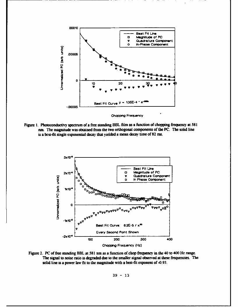
00010 -Best Fit Line* Magnitude of PC* Guadrature Component0 In-Ptse Component
.00005
0 0
S10 20 30C
Best Fit Curve Y - t35E-4 e•m--.00005
Choppng Frequency
Figure 1. Photoconductivy spectrum of a free standing BBL film as a function of chopping frequency at 581aun. The magnitude was obtained from the two orthogonal components of the PC. The solid lineis a best-fit single exponential decay that yielded a mean decay time of 82 ms.
3X10 4 [
3xIO'4 - Best Fit Line
2x10⁴ 0 Magnitude of PC- V Quadrature Componentj 0 0 In Phase Component
00 0
0 0
V•VVVVV VVVVVVV VV VVV9 VV0
V VVVVVV
SvvV Best Fit Curve: 8.2E-5 / x"V
Every Second Pont Shown-2x10'
100 200 300 400
Chopping Frequency (Hz)
Figure 2. PC of free standing BBL at 581 nm as a function of chop frequency in the 40 to 400 Hz range.The signal to noise ratio is degraded due to the smaller signal observed at these frequencies. Thesolid line is a power law fit to the magnitude with a best-fit exponent of -0.93.
39 - 13

.00
Data was fit to:
0
104 741 0.097 71n661 0.042 U6 y581 0.054 0 61n501 0.050 V 581 nm421 0.051 E3 501 nm
0 421mn
10 20 30 40
Chopping Frequency (Hz)
FIgure 3. Phatoconductivity as a fucution of chopping frequency for various wavelengths of the thin BBL samplecast on glass. T7he data w-as obtained w~ith a bia of 9 V. The data has been fit to a single decayingexponential, and the resulting best-fit decay time is giveni in the inset table.
39 - 14

Al aiivmn war fit to vna/Maaver the aI1S of 40 to200 NZ
¶ 0.3672 0.630
3 0.732
e7 0.670
V- A Scant Eeyacn dat 0ci iw 0
Sco
Svrth am 40 toa
50 100 200 400Chappbkg Frequency (Hz)
Figure 4. Thea sames ePermn of Figue thirepeatedpon thet was dayto 1 t625. The sampl hadoben xosdthe ligtof
poWe law chpis engt b txwo rangment Tm hw ninraehe PC drppdwihtah successive scans. The beo-it ieaexponent areg gituven inrthe inveset tablera. The fauexapaonets 350 Hzise qinte poinsent tandle.rdcbe
39AM1

.3S90.0 V* 67.5 V* 50.0 V+ 37.5 VA 25.0 V
m 15.0OV. 10.0V.2V 5.00V0 2.50V0 o 1.50 V
C
0
4-
0o .1z,-
0
1.5 20 2.5 3.0
Photon Energy (eV)
Figure 6. Field effect for the BBL on glass sample. The data has been noimalized for incident photon flux, and for
the applied bias. yielding per incident photon. There are significant differencesbetween successive spectra in both amplitude of the 1.8 eV feature and the relative intensity of the 3 eVshoulder compared to the 1.8 eV peak.
39 - 16
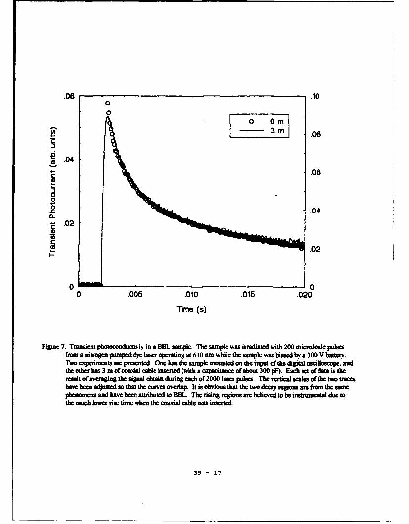
.06 .1000 0o 0
.08
.04
.06
0 .04
- .02
CS
S.02
0 00 .005 .010 .015.0
Time (s)
Figure 7. Transient photoconductii in a BBL sample. The sample was irradiated with 200 microjoule pulsesfrm a nitrogen pumped dye laser operatnug at 610 am while the sample was biased by a 300 V battery.Two exemet wre presented One has the sample mournted on the inpu of the digital osciloscope, andthe other has 3 m of coaxial cable imertd (with a capacitance of about 300 pF). Each set of data is theresult of averaging the signal obtain during each of 2000 laser pulses. The vertical scales of the two traceshoce been adjusted so that the cuve orverla. It is obvious that the two decay regions wre from the samepimszens and have been attributeda to BBL. The rising regions we believed to be intumna due tothe much lower rise fame when the coaxial cable was inserted.
39 - 17

"APIXX
IZPZX RTAL CAPABILITT ZMN1NMCNT
Photoconductivity
Previously, a "building block" photoconductivity (PC) system had been
assembled to demonstrate the viability of PC measurements on prototype
conducting polymers such as BBL 7 The previous apparatus was serviceable, but
required much user interaction, and lacked the capability of automated data
acquisition. Based on the success of the earlier study, newer building blocks
were procured that offered the possibility of automated data acquisition. The
existing one meter monochromator was replaced by a 0.5 meter monochromator
with double the optical throughput of the larger unit. The new Spex 500M
monochromator came with a "smart" controller and data logger unit. The smart
controller was used to communicate with the data logging and control computer
via a RS-232 interface. The computer is capable of setting the monochromator
to any wavelength and controlling the scan.
The lock-in amplifier was upgraded to an IEEE-488 compatible, dual
phase unit with a matching current to voltage preamplifier. The new system
greatly reduced the electrical noise in the observed PC data. The PC signal
is sent to the computer via the IEEE-488 bus. This lock-in also offers
control of its settings via computer, and most importantly, verification of
the current settings at the time of data acquisition. The digital to analog
output (DAC) has been used to control the rotational rate of the SRS model 540
chopper, allowing a new level of experimental flexibility.
The existing tungsten-halogen lamp was supplemented with a xenon short
arc lamp and power supply to provide greater light output in the blue to near
ultraviolet wavelength ranges where the signal to noise ratio rapidly
decreases. The data analysis-programs must take into account the intensity
profile of each light source before normalized conductivity spectra can be
generated from the raw data.
The new system has been set up to average a number of data values at
given wavelength increments. The new program offers two distinct
improvements: the user is certain of the wavelength, and the averaging
39 - 18
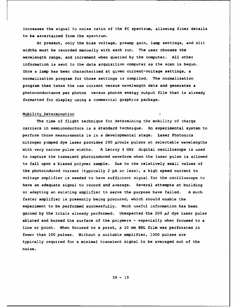
increases the signal to noise ratio of the PC spectrum, allowing finer details
to be ascertained from the spectrum.
At present, only the bias voltage, preamp gain, lamp settings, and slit
widths must be recorded manually with each run. The user chooses the
wavelength range, and increment when queried by the computer. All other
information is sent to the data acquisition computer as the scan is begun.
Once a lamp has been characterized at given current-voltage settings, a
normalization program for those settings is compiled. The normalization
program then takes the raw current versus wavelength data and generates a
photoconductance per photon versus photon energy output file that is already
formatted for display using a commercial graphics package.
Mobility Determination
The time of flight technique for determining the mobility of charge
carriers in semiconductors is a standard technique. An experimental system to
perform those measurements is in a developmental stage. Laser Photonics
nitrogen pimped dye laser provides 200 gJoule pulses at selectable wavelengths
with very narrow pulse widths. A Lecroy 4 GHz digital oscilloscope is used
to capture the transient photoinduced waveform when the laser pulse is allowed
to fall upon a biased polymer sample. Due to the relatively small values of
the photoinduced current (typically 2 pA or less), a high speed current to
voltage amplifier is needed to have sufficient signal for the oscilloscope to
have an adequate signal to record and average. Several attempts at building
or adapting an existing amplifier to serve the purpose have failed. A much
faster amplifier is presently being procured, which should enable the
experiment to be performed successfully. Much useful information has been
gained by the trials already performed. Unexpected the 200 #J dye laser pulse
ablated and burned the surface of the polymers - especially when focused to a
line or point. When focused to a point, a 10 mm BBL film was perforated in
fewer than 100 pulses. Without a suitable amplifier, 1000 pulses are
typically required for a minimal transient signal to be averaged out of the
noise.
39 - 19

A High Voltage One-Shot Switch Implemented With a FET Current Source and
Avalanche Diode
Thomas A. Baginski
Associate Professor
Department of Electrical Engineering
Auburn University
200 Broun Hall
Auburn University, Alabama 36849-5201
Final Report for:
Summer Research Extension Program
Wright Laboratory
Sponsored by:
Air Force Office of Scientific Research
Boiling Air Force Base, Washington, D.C.
and
Auburn University
September 1993
40-1

ABSTRACT
The description of a novel circuit which utilizes a FET current
source and high voltage diode to realize a simple, inexpensive, one shot
high voltage switch is presented. The switch was specifically designed
for slapper detonators or other applications where speed, low cost and
small size are important. The circuit readily lends itself to
implementation in either a discrete component, hybrid or monolithic
integrated circuit.
40-2

1. Introduction
High voltage switches capable of operating at high speeds are used
in a variety of applications. Typically, these switches are triggered
spark gap tubes which have a useful lifetime of several hundred to
several thousand firings. These configurations are expensive and bulky
when compared to a hybrid or monolithic integrated circuit. Also, in
some applications the ability of the switch to operate repetitively is
not required. The initiation of an explosive is one such example since
the switch is destroyed in the blast.
Slapper detonators are one application which require a fast ( i.e.
low impedance) high voltage switch. This report discusses a low cost,
low impedance, small, high voltage switch which is intended to actuate a
slapper. The circuit could be manufactured in a discrete component,
hybrid or monolithic integrated circuit which would make the
configuration especially applicable for use in large volume miniature
firing units.
2. Circuit Configuration
A schematic representation of one embodiment of the circuit is
shown in Figure 1. The configuration consists of a high voltage diode
DI. a series low resistance load R and a current source comprised of
QV, Q2' Rref and switch S.
The operation of the circuit is straight forward. The high voltage
capacitor CI is charged through resistor RC to a high voltage potential.
The function of the switch is to allow the capacitor to discharge
through RL quickly. This requires the current path between CI and
ground to be changed from a high impedance to a low impedance state as
quickly as possible.
The initial biasing point of DI is described by
IRA =IR (1)
40-3

where IRA is the actual current near the breakdown voltage, IR is the
normal reverse bias current of the diode with no avalanche effect, and
M = 1(2)
1 - (VR/BV)n
where M is the multiplication factor, VR is the reverse bias, BV is the
breakdown voltage and n has a value between 3 and 6. A plot of a
typical characteristic is illustrated in FIgure 2.
Diode DI is biased at a value of the breakdown voltage BY. At this
point the diode will permit any level of current to flow through it. In
order to insure that thermal runaway of the junction (which would damage
the device) does not occur it is necessary to externally limit the
current to a low level. The current source consisting of Q1 , Q2 and
Rref provides this function.
In the particular circuit that was tested the transistors were
matched high voltage n-channel MOSFETs. The equation which relates the
drain current (I D) in the devices to the gate to source voltage (Vgs
assuming the device is in the saturation region is
ID = K(Vgs - Vt) 2 (3)
where K is constant and Vt is the threshold voltage of the device.
Since the gate to source potential of both transistors is identical the
drain currents of the devices are approximately equal. The value of
ID is
ID -- [(supply V gs R ref (4)
Equations I and 3 can be solved simultaneously to yield the gate to
source voltage which is required to ensure the diode is on the edge of
avalanche breakdown. This V can then be substituted into equation 4gs
to yield the value of Rref to achieve this.
The switching of the configuration is initiated by closing switch
S. The supply voltage is then directly coupled to the gates of the two
transistors. The high potential on the gate Induces a channel region of
40-4

very low resistance between the drain and source which essentially
connects the drain of Q to ground. The entire potential of the
capacitor CI is then imposed directly across diode D1 which drives the
current through the diode to an extremely high value. The reverse
biased junction absorbs energy equal to the power integrated over time.
This value is approximately equal to
Q t VBV x I(t) x dt (5)
where Q is the approximate coupled energy (V x I x time).
The change in temperature of the affected volume of the junction of
the diode can be calculated from
AT- Q (6)CV
and
CV = PVC (7)
where CV is the heat capacity of the volume of silicon, p is the density
of the silicon (2330 kg/m3 ), V is the volume of the affected area of the
junction and C is the specific heat of silicon (712 J/kgK).PAssuming the junction of the device is of typical dimensions used
in a standard microelectronic process the effective power coupled to the
junction can easily be several thousand watts. The calculated
temperature change for such a structure is orders of magnitude greater
than the evaporation temperature of silicon (2680 C). What physically
occurs is the generation of a plasma arc which consumes the junction.
The plasma acts electrically as a short circuit between the top metal
contact of the diode and the device substrate. Thus, the diode has been
altered to act as a closed switch with very low parasitic impedance.
Once the diode junction has made its transition to the plasma state it
acts as a short circuit with an extremely low impedance. The voltage
potential of CI is now coupled directly to the drain of QI' The
magnitude of this voltage is greater than the potential necessary to
cause breakdown between the drain and source of transistor Q1. Once
breakdown occurs, essentially a short circuit exists between DI and
ground. Thus, a low impedance path exists for charge to flow from C1
40-5

through RL to ground.
3. TEST CONFIGURATION
The circuit was connected to a stripline to demonstrate proof of
concept. A high voltage power supply was used to establish a potential
of 2500 volts on the anode of diode DI. A commercially manufactured
diode with a measures breakdown of 1300V was utilized. However, device
parameters (i.e. junction area, interconnect metallization etc.) could
easily be optimized for this particular application.
A slapper was fabricated on an alumina substrate as illustrated in
Figure 3. Alumina is the most commonly used substrate material in
hybrid microelectronics, is very inexpensive, and has the widest range
of compatible manufacturing materials such as conductor and resistor
pastes available. The metal bowtie was screen printed onto the surface
using a palladium-silver conductor paste. Over the metal layer a glass
dielectric was printed to build up the barrel. A flyer was constructed
by applying polyimide into the barrel and then curing *the material.
Leads were then soldered to the ends of the slapper to permit electrical
connection.
The high voltage transistors chosen were standard DMOS elements
which are readily available commercially. The measured breakdown
voltage between drain and source was 1050V. The switch S was a low
impedance mechanical switch.
To demonstrate operation of the circuit switch S was closed and the
current flowing through the slapper was measured as a function of time.
The current reached a value of 3550A in approximately 150nsec. The
bowtie was evaporated and a typical arc was observed. The relatively
slow performance of the switch was probably due to the large inductance
in the leads of the firing circuit.
4. Hybrid Slapper/Switch Configuration
It is to be noted that an alumina substrate could be utilized as a
mounting vehicle for the entire circuit. A conventional slapper could
be easily fabricated by depositing a thin metallic film (via e-beam
evaporation, sputtering etc.) and patterning the film with conventional
40-6

microelectronic photolithographic techniques. A suitable dielectric
flyer material would next be deposited and patterned ( i.e. polyimide,
printed ceramics, glass etc.) The thicknesses and dimensional
tolerances of the configuration are easily met by these techniques.
Preliminary calculations indicate than a simple planar
metal --oxide-semiconductor capacitor could be fabricated by thermally
growing an oxide layer on a low resistivity silicon substrate. This
element could be made of a particular geometry to minimize parasitic
impedance and attached to the substrate by reflow soldering.
The advantages of constructing the slapper and firing circuit on
the same substrate as the switch and high voltage capacitor are
numerous. This arrangement would minimize the size of the entire
assembly since only one mounting vehicle is required for all components.
This reduces the number of packaging steps used in the manufacturing
process which reduces cost and increases reliability.
The length of the conductive paths between components is minimized
since the electrical components are as close together as physically
possible. The minimum lead lengths results in minimizing parasitic lead
inductance and resistance which reduces the discharge time of C .
Also, since many connections are printed onto the substrate and
fired/sintered simultaneously, reliability of the interconnect is
greatly enhanced. All solder connections can be realized by using a
conventional belt solder reflow station.
Technically it would possible to integrate the components of the
switch and charging capacitor on a monolithic substrate.
Microelectronic fabrication techniques are capable of producing large
numbers of devices economically.
40-7
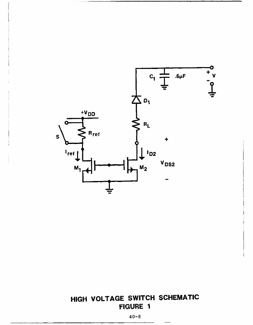
Cl .L .6p.F +v
DI
+VDD
s ~R ref 4
'ref 4•t V D2
VDS2
HIGH VOLTAGE SWITCH SCHEMATICFIGURE 1
40-8

BV
0 V
THE i-v CHARACTERISTIC OF A JUNCTION DIODEFIGURE 2
40-9

FIGURE 340-lo

Sivasubramanya Balakrishnan's report was unavailable at time of publication.
41-1
The Integration of J-MASS With MSTARS
Larry A. BeardsleyAssistant Professor of Mathematics
Department of MathematicsWaters Hall
Athens State CollegeAthens, AL 3S816
Final Report forSummer Faculty Research Program
Wright Laboratories/MNGSEglin Air Force Base, FL 32S42-S434
Sponsored by: Air Force Office of Scientific ResearchBoiling Air Force Base, Washington, D.C.
September, 1993
S~42-1

Integration of J-MASS With MSTARS
Larry A. BeardsleyAssistant Professor
Department of MathematicsAthens State College
Athens, Alabama
Abstract
The J-MASS architecture is a relatively new modeling system
designed to support engineers, model developers, analysts and decision
makers. It implements a series of standards and provides software tools to
support the development, configuration, operation and analysis of models
and simulations at varying levels of complexity and detail. MSTARS
(Modular Simulation Tools and Resources) is a joint project being
conducted by WL/MNSH and WL/MNMF using a collection of missile
simulation and analysis tools that is based on the Modular Missile
Simulation (MOMS) taxonomy currently also under development by the two
branches and based on the J-MASS simulation architecture. The
architecture Is being developed at Wright Patterson Air Force Base by
ASC/RWWW and WL/AAWA-1. J-MASS is written in the object-oriented
DOD-standard language, Ada, and is designed to be transportable between
different hardware configurations and to operate with any workstation
using a Posix-compliant Unix operation system. The initial capability of J-
MASS is limited compared to the total system specification,but a Fall 1993
release will provide functionality throughout the SSE, allowing a user to
log onto J-MASS and develop components, assemble them into models,
configure a simulation scenario and place players within the scenario, and
to execute the simulation and analyze the results through post-processing.
However, at the present time the WL/MNSH and WL/MNMF branches are
studying the new architecture to ascertain how the current 3DOF and 6DOF
missile code can be integrated with the recommended architecture.
42-2

The Integration of J-MASS With MSTARS
Larry A. Beardsley
1 Introduction
This report is a brief description of J-MASS (Joint Modeling and
Simulation System) architecture and its utility in the integration with the
MOMS (modular missile system) taxonomy under the MSTARS (modular
simulation tools and resources) effort.
The J-MASS architecture has been developed over a period of several
years and was designed to serve as a standard modeling and simulation
support system for use in the development of validated digital models of
threat and friendly systems and analysis of those systems. It was targeted
to support diverse simulation needs including system acquisition and
development, test and evaluation, the intelligent community, and for
training purposes.
A collection of missile simulation and analysis tools based on the
MOMS taxonomy are currently being developed In the WL/MNSH (Wright
Laborabory/ Munitions Simulation and Assessment) branch based on the
J-MASS simulation architecture being developed by ASC/RWWW and
WL/AAWA-1. These tools can be used by all directorate organizations as
well as outside organizations. The tools are being developed for both Unix
and PC environments. The MOMS architecture and taxonomy will
dramatically Improve the capability of organizations for building and
sharing missile simulations and subsystem models. It will be a reuseable,
extendable set of missile subsystem model specifications in Ada, allowing
diverse simulations to be built using compatible subsystem parts.
However, in order for the missile code using the MOMS taxonomy to be
efficient it must be based on an appropriate architecture.
The development of J-MASS began in the last quarter of 1990. The
version of the tool to support the partitioning task of model development is
completed. This tool supports production of object orientated design with
assemblies (OODA) drawings used in all J-MASS models. These OODA
drawings provide the major Input to the J-MASS code generator, of which
the 1.0 release was available earlier this year. The initial capability of
42-3

J-MASS Is limited compared to to the total system capability, but the full
2.0 release with code generator will be available by the end of calendar
year 1993.
The MNSH branch has been studying the J-MASS code to understand
the architecture and to ascertain how the missile code will be designed to
use the architecture most efficiently.
2 Problem Statement: J-MASS and Its Integration With MSTARS
The need for modeling and simulation becomes more important as the
complexity of our technology Increases and available funding for test and
evaluation decreases. In the Initial phases of R&D, it is Important to help
identify the best focus for technology minimizing expense. Once a set of
concepts has been formulated, modeling and simulation (M&S) Is effective
in identifying the critical performance Issues and selecting the best
concept for accomplishing technical goals, potentially eliminating the need
for multiple contracts and reducing the amount of hardware testing
required to select a best approach. During exploratory and advanced
development, medium to high fidelity models of a new technology should be
built to help determine whether weapon performance using the technology
justifies transition to Engineering Manufacturing Development (EMD).
Effective demonstrations of weapon performance to a customer using
quality simulations can be critical in selling the technology. During EMD,
M&S is used in both all digital and hardware-in-the-loop (HIL) forms to
support product improvement and augment the flight test program,
markedly reducing the number of flight tests required for proof of design
and as a result significantly reducing the cost of tear aind evaluation.
In the last few years, computer platfor-N have been Improving
greatly in performance while dropping sie- ý4.'antly in price. Also,
software engineering is being substantially i. ý.oved by such techniques as
object oriented programming and languages such as Ada 9X. As a result,
high fidelity and high speed simulation can be theoretically accniplished
today at an incredibly low cost.
However, there Is a problem. For years developed laboratory
projects required simulations from scratch, either by contract or in-house.
42-4

The result of this approach has been single use, non-related, non-
compatible software representing models of the technology being built
mated to some generic missile model or some simplified representation of a
real system. Unique simulations built from scratch are expensive and time-
consuming. It is difficult and near impossible to accurately predict missile
system performance based on technology models without using validated
simulations of the missile system being analyzed. Even if such simulations
exist, they are also unique and generally are not compatible with the other
simulations which have been developed. Also if other models exist, it Is
not possible to efficiently test another technology model which is not based
on the same architecture rendering it incompatible without significant
modification. Finally, when we transition our technology to be tested in
facilities such as the GWEF, high speed and high fidelity models of
portions of the system are required for hardware-In-the-loop (HIL) testing.
Using this approach, these models must be built almost from scratch to be
compatible with the unique real-time computer envirnment being used.
The solution to all of these problems is not a generic simulation
which supposedly can simulate anything. The diversity of components to be
modeled and the many ways they can be connected together makes it
impossible for such a simulation to exist. The simulations which have
attempted to do this were a compromise having a limited success in limited
application areas. The solution Is a common software architecture for
objects in general which are designed for Ada and an extendable taxonomy
of missile subsystem specifications in particular. A typical missile might
have subsystems interconnected as shown in Figure 1, page 42-6.
The objects shown in Figure 1 are connected In a specific manner,
but may be different for each missile being modeled. Also, some of the
components may operate differently with the environment In different
missile systems. For example, a radar seeker interacts with the
environment differently from an infared seeker. Also, different types of
radar seekers may behave differently and may provide different
information to other parts of the system. Obviously, what is needed Is not
a common missile simulation, but rather a set of reuseable components
42-5

w
W I-IILU
I- CC 0 L)
z p zf 00u
H 0.
LU w
0LL.2-
o 0ju CW-J0
C,0
~L.. ao Z LL
1.~- 0"~
which can be used to build different simulations based on unique
requirements.
The basic idea of an extendable taxonomy of missile subsystem
components is shown In Figure 2, 42-8. The objects might be organized by
mission area as shown in the figure or in some other manner. The idea Is
that libraries of objects can be built based on a consistent set of
component specifications. The specification only requires that the object
receive and provide data and function and procedure calls in a consistent
(specified) manner. The code which implements this Ada specification may
be anything desired and to any level of fidelity desired. For example, this
means that different kinds and fidelities of autopilot models can be built
using the same autopilot specification. If an autopilot model is needed for
which the specification does not exist, a new class of autopilot is invented
and added to the library. From the library, objects from the library can
be interconnected as needed to produce a missile model defining a
particular system.
The MOMS specification, being developed under the MSTARS work
unit, will provide an initial taxonomy which can be used by the Armament
Directorate and other agencies, and it can be extended indefinitely.
In fulfillment of the need for a new architecture, a project was
undertaken by ASC/RWWW to develop a Tri-Service simulation
environment Including a graphical user interface and a standard software
architecture for components which can be developed by any organization.
The project was undertaken in 1990 with the program goals of providing
the Department of Defense with the structure and software necessary to
reduce modeling and simulation development and operation costs, of
increasing the performance and credibility of models, and of increasing
responsiveness to user requirements and decreasing duplication. The J-
MASS programs office coordinates the development of the standard
architecture and modeling system in response to Tri-service requirements.
The problem in using J-MASS is that it Is written in a relatively new
language, Ada, and the architecture has been in a beginning evolutionary
stage up until release 2.0 a few weeks ago. The architecture of the earliest
release was not flexible enough to handle the current modeling
requirements of WL/MNSH. Also, the differences between the current 2.0
release and the earlier release are great. As a result, until now learning
42-7

MISWOATI PutS"S AL
TMACK GLAVE
WPOSMATW* ACCS& CuuNANIENGAG THEU*T
8T? TURN MATE- KT lOOT ACCEL
:' ALTITUOE & "Ah
STATUSTHESIS?
MACN A ATIMOS
Twa
VBLOaTY ALTITTUDE
Figure 2
42-8

the structure of J-MASS was not very beneficial to the integration effort.
In addition, the J-MASS code is voluminous. However, again, It Is
anticipated that the advantages, both in time and expense, will far
outweigh the initial time spent In understanding the code and in developing
it.
For reasons given later in this paper, J-MASS was chosen as the
architecture upon which to integrate with MOMS. Since J-MASS was not
designed in-house, the architecture needs to be studied and understood
before its integration with the 6DOF missile code. My task was to aid in
both the studying of the architecture and in the impi.mentation of the
6DOF code. However, the J-MASS release which WL/MNSH wanted to
study was not delivered until a few weeks before my summer tenure ended.
However, the time was well spent in both learning about object-oriented
programming and in studying previous releases of J-MASS. Since receiving
the release, some of the data flow has been examined and discussed in this
paper. However, I felt it would be instructive to first give a brief history
of the J-MASS architecture and why it was chosen as a model, and why
Ada was chosen as a language.
3 Why Was Ada Chosen As a Language for the Design of J-MASS
In considering Ada as a language, the _v-MASS program office wanted
a language that was understandable, reliable, efficient, and easily
modified. The language of Ada is patterned after the engineering
principles of abstraction, information hiding, modularity, localization,
uniformity, completeness, and confirmability [1). In addition it was
desired that the language support object oriented programming. According
to Booch, object oriented programming is a method of Implementation in
which programs are organized as cooperative collections of objects, each of
which represents an instance of su;ne class, and whose classes are all
members of a hierarchy of classes united through inheritance relationships.
An Important aspect of object-orientedness is that it uses objects rather
than algorithms as its fundamental logical building blocks. One of the
benefits of object oriented programming Is that It helps exploit the
42-9

expressive power of all object-based and object-oriented languages which Is
conducive to achieving significant improvements in productivity and code
quality. Secondly, it encourages reuse not only of software but of entire
designs. Thirdly, it produces systems that are built upon stable
intermediate forms that are resilient to change. Fourthly, it reduces the
risk of developing complex systems. Most importantly, It appeals to the
workings of human cognition.
A comparison of FORTRAN, Ada, and C++ was made by WL/MNSH
based on the software engineering principles of Booch. As a result, the
choice was narrowed down to Ada or C++. Ada and C++ both have good
data abstraction and information hiding capabilities, but Ada was
considered to be more readable and understandable than C++.
4 Why J-MASS As a Simulation Architecture?
Now that a language had been decided on, an architecture needed to
be chosen which would take advantage of Ada's assets. The architecture
had to support the following:
a. object oriented programmingb. reuseable, reconfiguration simulation componentsc. multiple level, diverse types of simulation componentse. automatic code generation
In addition it had to provide for loose coupling between components,
produce fast executing code, and be attractive to a large base of users.
Some of the simulation architectures reviewed were GENSS, TRAP, WISM,
HAVE SLICK, HADAMS, TAP, AMRAAM (Litton heritage), Carnegie
Mellon Software Structural Model, and JMASS. In deciding these choices,
it was decided that:
(1) Litton, GENSS, AMRAAM, TRAP, and SIM all have high coupling,
limited component reuseability, and do not support automatic code
generation or object-oriented programming. Also, direct translation into
Ada would not offer any advantages over FORTRAN since the desireable
features of Ada would not be used.
42-10

(2) Developing our own architecture would be laborious and cost
intensive.
(3) Carnegie Mellon's software architecture should lend itself to time
intensive models which can be allocated to a separate processor. Current
simulation architectures are difficult to modify for accomplishing this. It
was desireable for the chosen architecture to be widely used. This would
promote widespread sharing of parts and lower verificatluu and validation
costs for components.
(4) J-MASS, which uses a form of Carnegie Mellon"s SSM meets most
requirements, and WL/MNSH will inherit products currently being
developed.
With these possibilities, J-MASS was selected with Carnegie Mellon's
SSM architecture decided upon as a backup architecture. The branch
will make the best use of older FORTRAN simulations as a guide to
effective numerical algorithms and subsystem completeness.
Two of the architectures, J-MASS and the Litton approach, are
compared. The strong points of the Litton approach are:
(1) it is organized for building simulations.
(2) modules represent subsystems of the weapon as do modern object
oriented approaches.
(3) modules werp designed to be as independent as possible except for the
C-array.
(4) use of "equivalence" statements with C-array resulted in some
improvement for data visibility, modifiability, and I/O flexibility over
other FORTRAN programs using only common blocks.
The weak points of the Litton approach are:
(1) Objects are not clearly separated (e.g. missile processor processing
"real world data").
(2) Attributes are not clearly distinguishable in each subroutine (loosely
defined objects).
(3) Subsystems are not truly reuseable in other simulations without code
42-11

modifications. (that is, they are hardwired to C-array)
(4) maintenance of C-array is a collosal task for the simulation
configuration manager.
In comparison, the strong points for the J-MASS approach are:
(1) Ada language was used and implemented to best use Ads features.(2) Components are reusable and reconfigurable in another system without
code changes.(3) diverse types of simulation components are supported.(4) objects are loosely coupled and highly cohesive.(5) arbitrary levels of fidelity are possible.(6) allows arbitrary level of component decomposition.(7) all objects have the same basic structure.(8) outstanding data accessibility through the use of pointers exfsts.
The weak points of J-MASS are:
(1) the flexible simulation design is less runtime efficient.(2) making model component building and configuration simple requires
sophisticated simulation facilities and utilities including a datamanagement package and a service Interconnect backplane.
In addition to Its strong points, J-MASS has the potential for
becoming a widely used standard which in turn would promote large scale
component sharing, and simulations could be understood by many. Also, we
would Inherit tools being developed by J-MASS such as the graphical run-
time environment, graphical model building with the automatic Ada code
generator, 3-D animated graphics for simulation visualization, and data
plot capability.
5 What Is J-MASS?
J-MASS is a modeling system designed to support engineers, model
developers, analysts and decision makers [2]. It Implements a series of
standards and provides software tools supporting the development,
configuration, operation and analysis of models and simulations at varying
levels of complexity and detail. Additionally, J-MASS provides a library
of verified software components for the model designer to use, and J-MASS
models are verified and validated before they are placed In this library.
42-12
Formal configuration managagement ensures the library retains its
integrity. J-MASS is not a model; it is a system to develop and support
models developed in compliance to the basic J-MASS architectural
standards.
J-MASS supports models with an object-based design coded In the
DOD-standard Ada software language. It is designed to be transportable
between different hardware configurations and is built to operate with any
workstation using a Posix-compliant Unix operating system. J-MASS uses
an open systems approach. Standards are specified wherever possible,
enabling J-MASS software to interface with other standard software.
One of the key parts of J-MASS design is the SSM (Software
Structural Model). It identifies standard interfaces with the Simulation
Support Environment (SSE) and uses information with standard formats.
Rather than forcing a modeler to do more work, it tells the modeler where
to place different attributes of the individual objects, encouraging
standardization. With respect to the SSE, objects are processed in the
same manner, and information Is provided to the object when its state is
updated and the object provides information back to the SSE. As a result,
the designer can focus attention on designing the algorithms needed to
describe what is bIeing modeled rather than on the style of the model.
When developed, the J-MASS code generator will be used to transform the
algorithms into actual Ada code compliant with the J-MASS software
structural model.
J-MASS includes the SSE and the modeling library as described in
Figure 3, Figure 42-16. The SSE supports the modeler in accomplishing
any or all of five basic functions.
(1) develop model components
(2) assemble model components into a model
(3) configure simulation scenarios for execution
(4) execute the scenario and generate data
(5) post-processing of the data
5.1 Develop Model Components
The first step in developing a J-MASS system model Is to partition
the system Into its components. The process continues to the level the
42-13

modeler needs to provide the detail appropriate to the task, whenever
possible maintaining a one-to-one mapping from the physical world to the
simulation being maintained. For example, a design engineer may partition
a radar system into individual gates and amplifiers in the circuitry, while
a systems analyst may decompose the radar into only the transmitter,
processor and receiver. Thus, the system support environment allows
model development to match the needs of the modeler without forcing detail
beyond that which is required.
5.2 Assemble Model Components
After a developer partitions the system into its components, a library
of already developed objects can be accessed. For example, if a design
engineer needs a model of a gate, he simply accesses the library, browses
through listings and descriptions of the gates in the library and retrieves
the one that matches the need. The specific attributes for that object are
"tailored" for the specific application. The engineer has now Incorporated
an object developed and validated by another modeler. The developer has
saved time and money and is assured of a quality product since all of the
objects in the library have been evaluated.
Usually, in a given simulation, many objects are used over and over
in varying configurations but with unique data, called attributes, to
produce very complex models. The model parts are easily connected using
the J-MASS architecture.
5.3 Configure Simulation Scenarios
After a model is developed, it can be placed in a simulation scenario
where the scenario is a "one-on-one" simulation or a "few-on-few"
simulation where the focus is on system Interaction.
J-MASS allows for the models in the simulations to be placed in
specific physical locations. Terrain is modeled based on data from the
Defense Mapping Agency. Appropriate geography, atmosphere, surface
cover and other factors are added to the scenario.
42-14

J-MASS is also being developed to support simulations Involving"many-on-many" player interactions. These scenarios will usually involve
lower detail J-MASS models due to the scenario complexity.
5.4 Execute the Scenario
During the setup, the operator specifies the data required for
subsequent analysis. Upon execution, the scenario is played out and the
data is captured in files for analysis. With real-time applications, data
will be available for instant viewing.
Also, modelers can execute complex scenarios using several different
models, knowing that individual models will interact properly since each is
designed and built to the same standards.
5.5 Post-processing
J-MASS supports an extensive analysis capability in the post-
processing phase. For example, in an emulative radar model, the design
engineer can actually trace signals through a circuit. Engineering graphs
can be generated as well as tables, maps, traces of actual versus predicted
value, position, and almost any other representation of data.
One of the benefits of J-MASS will be to allow engineers without
extensive software backgrounds to construct detailed models using a
concept called "visual programming". This concept will allow for the use
of standard engineering notation to design a model where the code will flow
from the engineering.
42-15
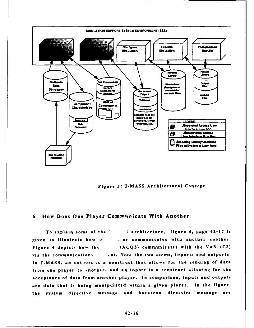
SIMULATION SUPPORT SYSTEM ENVIRONMENT (SSE)
GExamum Punt44 xnSimulation SIMuidin ReGulU
Ub.MTd~ Ubreyi~~a
SlmfeyMo £ Wee(ire.
6 o os n lye om ndiate oeWithl Anthe/1krJ
Toepansoi fte waciectur, oe, iue4 ae4-7i
gvn t ol anther aohr
Figure 4 depicts how the (ACQ3) communicates with the VAN (C3)
via the communications •nt. Note the two terms, inports and outports.
In J-MASS, an outport ,• a construct that allows for the sending of data
from one player to •nother, and an inport is a construct allowing for the
acceptance of data from another player. In comparison, inputs and outputs
are data that is being manipulated within a given player. In the figure,
the system directive message and backscan directive message are
42-16
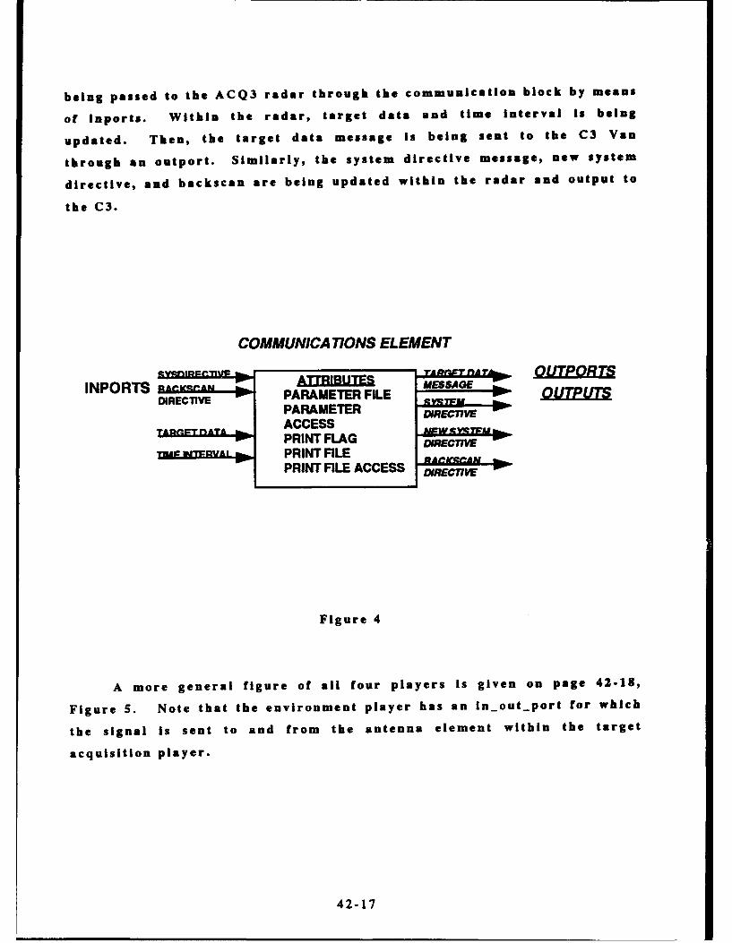
being passed to the ACQ3 radar through the communication block by means
of Inports. Within the radar, target data and time interval is being
updated. Then, the target data message is being sent to the C3 Van
through an outport. Similarly, the system directive message, new system
directive, and backscan are being updated within the radar and output to
the C3.
COMMUNICATIONS ELEMENT
jYnRrEllr=9IE ATRBUE rd - WJr ArANMWTUPO
INPORTS Prsa ESGDIRECTPVE PARAMETER FILE QITIM ,.TM
PARAMETER DIRECTIVE
TAQP.I=T nATA ACCES NFW-Qt•'rW1M-• PRINT FLAG DIRECTIVE
T W F: W. • = Av I& p oll P R INT F IL ER A -Of C r A
PRINT FILE ACCESS DIRcnVE
Figure 4
A more general figure of all four players is given on page 42-18,
Figure 5. Note that the environment player has an inout-port for which
the signal is sent to and from the antenna element within the target
acquisition player.
42-17

INTER-PLAYER COMMUNICATIONS
Tgt Mrcraft Player ENV E. . -nint Playei
Out~por1 CO*0 IN-PORT iN_OUT-PORT I •lOuLport
adfOuo b: IN, I
Emftc DeihibEmnrw isld"ihehIn~ f.,istw •It
cCC Conmmand, Control Acq Target Acqulaionand Radar Player
Communicalons VanPlayer Communloatons Antma
Element ElementOULYORT s' IN-PORT OUTPOr'OUT-PORT Bechmm Ofreo~ I• IN-PORT
IN -PORT Target n.. OUTPORT
Figure 5
6 Concluding Remarks
New weapon technology is very complex, diverse, and software
intensive. Previous simulations had very limited flexibility for handling
these requirements. Technology design comparisons require simulation
module Interchangeability, and many simulation architectures are
somewhat rigid. Many of them are written in FORTRAN, a language whose
supersets limit transportability. Rapidly changing requirements demands
that software be easily modified. The new simulation architecture, J-
MASS, is a viable alternative for all of the reasons mentioned in this
report. Previous simulation architectures were not sufficiently robust for
optimal modeling of different weapon subsystems at multiple levels of
fidelity. Also future simulation needs includes distributed components for
42-18

networked integrated technology testing. An appropriate simulation
architecture should lend itself to time Intensive models which can be
allocated to a separate processor. J-MASS, an architecture which utilizes
the object oriented approach based on Ada, offers a means to accomplish
the given objectives whereas others are difficult to modify for
accomplishing this. It is conjectured that the J-MASS architecture will be
widely used, and this would promote the widespread sharing of parts and
would lower verification and validation costs for components.
The WL/MNSH branch and myself learned a great deal of the benefits
of the J-MASS architecture this summer. Although, there exist some
gliches, mostly hardware related, the capabilities offered by the
architecture and the time and money savings will outweigh the initial time
in both fully understanding its functionality and its integration with the
missile code. The development of the 6DOF code utilizing the J-MASS
architecture has already begun and should the functional In the near
future.
Acknowledgement
I am thankful to the Air Force Office of Scientific Research for
offering me the opportunity to conduct research at Eglin AFB, Florida. In
particular, I thank all of the personnel of the simulation and assessment
branch of the armament directorate for both their encouragement and the
affording of all the documentation and software to aid me in my study of J-
MASS and the Ada language. Thanks to Capt. Patti Eggleston for the time
she spent in helping me with a new word processor in typing this paper and
In our study of a target model, to Capt. Eric Scarbrough for his studying of
some of the J-MASS with me and in suggestions for the diagrams, to Tim
Pounds for his accessibility for answering numerous questions and
providing documentation and system support, and to the Branch manager,
Larry Lewis for the use of some previous documentation. Many thanks to
everyone already mentioned and to Dr. Martin Moorman, Ed Moorman and
Yves Malette for making me feel welcome during my twelve week tenure at
Eglin.
42-19

References
[1] Grady Booch, Software Engineering With Ada, Benjamin Cummings,
Second Edition (1986)
121 Randy E. Brown and William K. McQuay, "The Joint Modeling and
Simulation System", Journal of Electronic Defense, September, 1992.
[31 Gary A. Whitted, "Software Development Plan (SDP) Volume II,
Software Structural Model (SSM) Design Methodly for the Modeling
Library Components for the Joint Modeling & Simulation System
(J-MASS) Program", Version 2.0, February 26, 1993.
42-20

INFLUENCE OF PENETRATOR AND TARGETPROPERTIES ON PENETRATION MECHANICS
E. Eugene Callens, Jr.Associate Professor
J. Scott McMurtryGraduate Student
Department of Mechanical andIndustrial Engineering
Louisiana Tech UniversityRuston, LA 71272
Final Report for:Summer Research Program
Wright Laboratory
Sponsored by:Air Force Office of Scientific ResearchBolling Air Force Base, Washington, D.C.
September 1993
43-1
INFLUENCE OF PENETRATOR AND TARGETPROPERTIES ON PENETRATION MECHANICS
E. Eugene Callens, Jr.Associate Professor
J. Scott McMurtryGraduate Student
Department of Mechanical andIndustrial Engineering
Louisiana Tech University
Abstract
A previously developed quasi-steady wave mechanics model for penetration
of structural targets is modified to include an improved model for the initial
and terminal transients. The improved model is then utilized in the
parametric study of the influence of penetrator and target properties on
penetration depth. The wave mechanics model not only predicts the trends in
penetration with variation in these properties, but it also delineates the
kinematic mechanisms that are responsible for these trends. It is shown that
the combination of high penetrator strength and low target strength produces a
local maximum in the plot of penetration depth versus impact velocity. The
wave mechanics model shows that the observed decrease in penetration depth
with increasing impact velocity is due to flow initiation in the high strength
penetrator. For high strength targets, the strength of the penetrator is
shown to have little influence on penetration depth. However, for low
strength targets, increased penetration results from increased penetrator
strength. The effect of penetrator L/D on the ratio of penetration depth to
original penetrator length is shown to be very pronounced for L/D's less than
6 but diminishing to near insignificance for L/D's greater than 12. The wave
mechanics model shows that the L/D effect is due entirely to the initial and
terminal transients. The effects of target strength, penetrator strength, and
penetrator density on penetration depth into concrete targets is also
presented.
43-2
INFLUENCE OF PENETRATOR AND TARGETPROPERTIES ON PENETRATION MECHANICS
E. Eugene Callens, Jr.J. Scott McMurtry
INTRODUCTION
The work reported in Ref. 1 indicates that excellent agreement with
experimental data is obtained for a properly formulated one-dimensional quasi-
steady wave mechanics model of the penetration processes for blunt,
cylindrical penetrators. The necessity of employing a wave mechanics model is
rooted in the observation that the total time for the penetration process
exclusive of the terminal transient is usually less than 200 microseconds.
The corresponding deceleration levels are typically more than one million
times greater than the standard value of gravitational acceleration. Thus,
the classical differential equations for rigid body mechanics cannot
adequately describe the time resolved response of either the penetrator or
target material.
A major advantage of a realistic model of the governing physical
mechanisms over a straight forward correlation of experimental data is that
the physically based model can delineate the processes that cause the observed
and predicted data trends. For example, the interaction between the
hydrodynamic flow stress and the structural stresses in the penetrator and
target dictate at what penetrator velocities flow is initiated in the
penetrator and/or target. The initiation of flow, in turn, has a dramatic
effect on the penetrator and target response as is illustrated in the
parametric studies reported below.
The current work employs a wave mechanics model to conduct a parametric
study of the effects of target and penetrator compressive strength and density
as well as the penetrator length to diameter ratio on penetration depth. The
study covers the entire velocity range from those values where penetration is
initiated and material strength effects are dominant to the hypervelocity
values where material strength effects are insignificant and the penetration
process is hydrodynamic in nature. The range of material densities and
strengths includes all engineering materials, and the penetrator length to
diameter ratios range from 1 to 50.
QUASI-STEADY WAVE MECHANICS MODEL
The quasi-steady wave mechanics model used in this study is presented in
Ref. 1 and summarized below. The governing equations are the conservation of
momentum, the conservation of mass, and a velocity component kinematic
relationship.
43-3

The penetrator/target interface momentum equation is
5 / + P / U2 Pr = P / u2 TF +S/P P T T
where
SI, = Stress in compressed penetrator
S, T = Stress in compressed target
pl, = Density of compressed penetrator
pl, = Density of compressed target
U,, = Penetrator flow velocity
UTP = Taiget flow velocity
The one-dimensional wave continuity equation in the penetrator is
VWPPP PP VWP - UPP (2)
and for the target
VPr PT VNT - UPT (3)
where
pp = Penetrator initial density
PT = Target initial density
Vp = Penetrator wave velocity
Vr = Mean target wave velocity in the bow region
UPP = Penetrator particle velocity
UFT = Mean target particle velocity
The particle velocity is the change in velocity associated with the
passage of the disturbance wave. The kinematic relationship between the
various velocity components is given by
VP = up, + UPP + U" + PT (4)
where V, = Velocity of the f ree end of the penetrator.
The velocities in the penetrator and target before and after the
disturbance waves are shown schematically in Fig. 1 relative to the interface.
43-4

The wave velocities are given by
VP = CP + SIP Upp (6)
where
CW = Zero pressure wave velocity in the penetrator
CW = Zero pressure wave velocity in the target
SIP = Hugoniot constant for the penetrator material
SIT = Hugoniot constant for the target material
The stress in the compressed penetrator is given by
S = P p pp Vwp for UPF = 0 (7)
/(8SP= PPUPP4VWP for UPF > 0 (8)
UppM - (9)
CSP = Vp (10)
where
Uppm = Maximum penetrator particle velocity
Csp = Penetrator free surface maximum stress constant
1), = Poisson's ratio for the penetrator material
asp = Penetrator compressive stress
From these relationships it is observed that either the penetrator
particle velocity or flow velocity is known for any condition. If the
interface pressure is below the maximum allowable penetrator stress, the flow
velocity is zero, and the particle velocity is the variable. If the interface
pressure is above the maximum penetrator stress, the particle velocity is at
its known maximum value and the flow velocity is the variable.
The stress in the compressed target is given by
S= PTUPTVwr for UTF = 0 (Ii)
ST P PTUPTmVWr for UTF > 0 (12)
43-5

C•TO _ , (13)PT VW
C, = c2 s = V-2T (14)
where
U'M = Maximum mean target particle velocity
C',r = Target confined surface maximum stress constant
C'r = Target free surface maximum stress constant
VT = Poisson's ratio for the target material
CY = Target compressive stress
As in the case of the penetrator, either the target particle velocity orflow velocity is known for any condition. The penetrator deceleration is
determined by the wave mechanics. In this model the compression wave that
originates at the penetrator/target interface upon impact is tracked in the
penetrator as it travels back and forth between the interface and the free
end. The compression wave reflects from the free end as an expansion wave and
the penetrator free-end velocity decreases by twice the particle velocity with
each reflection.
When the expansion wave reflects from the interface, the sum of the
penetrator and target variable velocities decrease by twice the particle
velocity. The new values of these velocities are determined from the
interface momentum equation and the velocity component kinematic relationship.
Again, the particle velocity changes sign with each wave reflection.
The penetrator traveling wave is tracked until the penetrator velocity
falls below the target flow initiation velocity. When this occurs the
developed penetration phase is complete and the remainder of the penetration
process is a terminal transient cylindrical expansion of the target stress and
a spherical expansion of the penetrator flow stress as presented below. The
change in penetrator length due to the developed penetration phase is
= -f( UpF± Up,) dt (15)
The change is crater depth due to the developed penetration phase is
ALM, f( UTF+Upr4dt- (16)
43-6

The final crater diameter at each penetration location is given by
/ -2(7DD-c= PP U PFc,, +S CST (,.%T ( 17 )
DP ~ CSTr UST
where D, = penetrator initial diameter.
INITIAL AND TERMINAL TRANSIENT MODELS
The initial and transient models have been modified from those presented
in Ref. 1. The time for the initial transient is taken to be the time for the
passage of the lateral release wave in the penetrator
A RP (18)
where
Vwrr = Penetrator transverse impact shock velocity.
The crater length due to the initial transient is given by
LcI UPTS - UPTM ) A tr 19
where
Us = Target shock particle velocity
The length of penetrator loss during the initial transient expansion is
obtained from a form of the velocity kinematic relationship
A Lp = -( VpI&tZT-LCI) (20)
The terminal transient model is a combination of a spherical penetrator
flow stress expansion and a cylindrical target particle momentum expansion.
The crater length due to the spherical expansion of the penetrator flow stress
is
= pCU2pC -_ (21)CST 0 ST
43-7
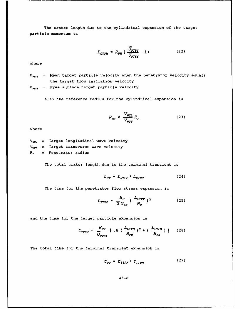
The crater length due to the cylindrical expansion of the target
particle momentum is
LCTrp = RPR UPTfl 1) (22)UFrPs
where
UPTI = Mean target particle velocity when the penetrator velocity equals
the target flow initiation velocity
U•,s = Free surface target particle velocity
Also the reference radius for the cylindrical expansion is
R VWrLRPR - - (23)
where
V,, = Target longitudinal wave velocity
Vu = Target transverse wave velocity
R, = Penetrator radius
The total crater length due to the terminal transient is
Lc. = LC(PF + Lc2PH (24)
The time for the penetrator flow stress expansion is
t TTPF - ( ) 2 (25)2 UpF Rp
and the time for the target particle expansion is
tT7pm =---RPR [ 5 ( LCTPM- ) 2 + ( LCFPM) (26)
UpTFZ R PR RPR
The total time for the terminal transient expansion is
tr = tTTPF4 + tT3- (27)
43-8

COMPUTATIONAL RESULTS
The above equations constitute a comprehensive model for the completeterminal ballistics process including the initial transient, the developedpenetration regime, and the final transient. The model predicts crater depth,
penetrator velocity, and penetrator length as a function of time as well as
the final crater diameter as a function of crater depth.
The equations have been programmed using the True BASIC language and the
program is readily solved on a personal computer. Typical run times are 15
seconds on a 25-MHz 386 PC with a math coprocessor.
Fig. 2 presents data in terms of the ratio of penetration depth to
original penetrator length (P/L) for tungsten alloy penetrators into rolled
homogeneous armor (RHA) targets. The calculated P/L results are compared withdata from Ref. 2 for length to diameter ratios (L/D) of 3, 6, and 12 andpenetrator impact velocities (VPI) from 600 to 1600 m/s. The predictions show
the experimentally observed L/D effects. Both the experiment and calculations
show a change in slope at an impact velocity of approximately 800 m/s. This
corresponds to the velocity at which the RHA target reaches the maximum
confined surface stress and begins to flow.
Fig. 3 shows the same agreement within the experimental uncertainty for
a mild steel penetrator into an aluminum target for L/D = 3. The experimental
data from Ref. 3 extend from an impact velocity of approximately 900 m/s where
target and penetrator strength effects are very significant to 5000 m/s wherethe penetration process is approximately hydrodynamic.
Figs. 4 and 5 compare the calculated results with experimental data from
Ref. 4 for tungsten into ST52 steel and a penetrator L/D of 10.4. Two
calculated curves are presented which correspond to the range of compressivestrength quoted for ST52 steel. Fig. 4 presents the comparisons for crater
depth, and Fig. 5 presents the comparisons for crater diameter. The agreement
is seen to be excellent over the entire velocity range from 600 to 3600 m/s.The effect of target strength on penetration depth for high and low
strength penetrators is shown in Figs. 6 and 7, respectively. Both plots show
increasing penetration with decreasing target strength as expected. However,
for the combination of high penetrator strength and sufficiently low targetstrength, Fig. 6 shows a local maximum in penetration depth occurring at
moderate impact velocities. The wave mechanics code clearly indicates that
this decrease in penetration depth with increasing velocity is due to flow
initiation in the high strength penetrator.
This phenomenon is further investigated in Figs. 8 and 9 where the
effect of penetrator strength on penetration depth is presented for high andlow strength targets, respectively. For high strength targets, the strength
of the penetrator has little influence on penetration depth (Fig. 8).
43-9

However, for low strength targets, there is significantly more penetration
associated with increasing penetrator strength at moderate to high impact
velocities (Fig. 9). The local maxima are present for all but the two lowest
strength penetrators. At impact velocities above 3,000 m/s, the curves are
seen to coalesce due to the fact that even the highest strength penetrators
are flowing under the influence of the high interface pressure. The
penetration depth continues to increase with increasing velocity above 3,000
m/s due to terminal transient effects.
The effect of target density on penetration depth is presented in Figs.
10 and 11 for high and low strength targets, respectively. At highvelocities, the penetration depth increases as target density decreases as
expected. However, the curves cross at low velocities indicating that there
is a regime where low density, high strength targets are more resistant topenetration than high density, high strength targets (Fig. 10). The wave
mechanics model shows that this is due to the higher target flow initiation
velocities associated with the lower target densities. This also suggests
that the superior penetration resistance of ceramics over metals at low to
moderate velocities may be due in part to the lower densities of the ceramicsin addition to the obvious advantage of higher compressive strengths. Fig. 11
also shows that the penetration local maximum phenomenon is very pronounced
for very low density targets.
Figs. 12 and 13 show the effect of penetrator density on penetrationdepth for high and low strength targets, resp.ectively. The anticipated
characteristic of increasing penetration with increasing density is observed
in both figures. Fig. 13 shows that the locai rn.xima occur for low strength
targets if the penetrator density is sufficiently large.
Fig. 14 presents the effect of L/D on penetration depth for L/D of 1, 3,
6, 12, 20, and 50. The penetrator and target material properties are typicalof a tungsten alloy penetrator into RHA. Low lues of L/D are observed to
have substantially high relative penetration compared to the higher L/D's.
However, as L/D increases the difference diminishes and becomes nearly
insignificant for L/D above 12. The wave mechanics model shows that the L/D
effect is due entirely to the initial and terminal transients. There is no
difference in the relative penetration of different L/D penetrators in the
developed penetration regime.
The effect of target strength, penetrator strength, and penetratordensity on penetration depth into concrete is shown in Figs. 15, 16, and 17,
respectively, for a penetrator L/D of 12. Fig. 15 illustrates that the
penetration depth has a local maxirr- tor concrete strengths below 20,000 psi
for a tungsten alloy penetrator. F.,r normal structural strength concretebetween 3,000 and 5,000 psi, the effect is quite pronounced. The consequence
43-10

of this phenomenon is that there is a limit on the impact velocity to achieve
maximum penetration in concrete. The same effect is observed in Figs. 16 and
17 for all but the two lowest penetrator strengths and densities.
It is concluded that the wave mechanics model is very effective in the
delineation of the effects of penetrator and target characteristics on
penetration mechanics. Not only are the trends in penetration depth appatant
but, more importantly, the physical mechanisms that drive these trends are
exposed. The mechanisms are dynamic in nature and produce results that may
not be anticipated from consideration of static material properties.
REFERENCES
1. Callens, E. Eugene, Jr. and J. Scott McMurtry, "One-Dimensional Wave
Mechanics Model for Terminal Ballistics," Final Report for AFOSR Summer
Research Program, Aug. 1992.
2. Tate, A., K. E. B. Green, P. G. Chamberlain, and R. G. Baker, "Model Scale
Experiments of Long Rod Penetration," Proc. Fourth Int. Symp. Ballistics,
Oct. 1978.
3. Christman, D. R., A. B. Wenzel, and J. V. Gehring, "Penetration Mechanisms
of High-Velocity Rods," Proc. of the Seventh Hypervelocity Impact Symp.,
Tampa, FL, Vol. V and VI, Experiments, Nov. 17-19, 1964.
4. Hohler, V., and A. J. Stilp, Penetration of Steel and High Density Rods
in Semi-infinite Steel Targets," Int. Symp. on Ballistics, 1977.
43-11

TARGET
U+ TF UT + U•
PENETRATOR
/i/
FIG. 1. FLOW AND PARTICLE VELOCITIES RELATIVETO THE INTERFACE
43-12

FIG. 2. TUNGSTEN INTO RHA, LID =3, 6, 121.4-6CL 1-~?
1.2 30-.EXP +. 6-EXP XI 12 -EXPJC
1...TATE ET AL,.............
0 .8 .- --- -- --- -- -- ---- -- -- ----- -- -- -- --- .. .. -- -- ... .. .. ---- -- --- -----
0~0
020
0*400 600 800 1000 1200 1400 1600 1800
VPI (mis)
FIG. 3. MILD STEEL INTO AL, L/D -=33.0-
0. . .. .......................... ,... ....................I......................
2 . ---------50 00 50 00 50 0035040040050050
...... ~V P (.. .... ..... ..... .. s )-- --
CL 1 5 ............ : ..... 3...3

FIG. 4. TUNGSTEN INTO ST52 STEEL, L/D = 10.4,CRATER DEPTH
1.6.
HOHIER REF 4
1.4. . . . . . ..---........ .... ....................... ..................
1.2.
-.. . ............. .....- . -540MPA, CAL ....680 MPA, CAL W EXP
500 1000 15ý00 2000 2500 3000 3500 4000 4500VPI (mits)
FIG. 5. TUNGSTEN ITO ST52 STEEL, L/D = 10.4,CRATER Dli 'ETER___ __ __ __
6.0- -
55 ............ ...... .---- .....
5.0. ERREF.
3.0
1.5 *---------- -L 540------- LA CAL . 680 .....CAL......
500....... 100 1500.... 2000 250.300.50.400.50----------V--- ..........----------..........)......
43-0

FIG. 6. EFFECT OF TARGET STRENGTH ON PENETRATION__DEPTH, HIGH STRENGTH PENETRATOR ____
3.5-. _ _ _ _ _ _ _ _ _ _ _ _ _ _ _ _ _ _
PENETRATOR DENSITY - 17120 K~43
3.0-- PENETRATOR STRENGTH - 1196 hIPA
2.5 GET DENSITY - 7900 G 1..............
2 . -------
PENETRATOR~L DE~fY 1722K
30 .. . . . . . ....... ...............----
0.5 .. .----.............. '..*----- O A . . ..........
0.5- .
0 500 1000 1500 2000 2500 3000 3500 4000 4500 5000VP! (m/s)
FIG 7 EFEC OFTAGE STENTH N4ENERAI5

FIG. 8. EFFECT OF PENETRATOR STRENGTH ONPENETRATION DEPTH, HIGH STRENGTH TARGET
3.5-PENETRATOR DENSfrTY 17120 W
LTARGET DENSIT - 790GM3
2.5-1TR E STRENGTH - 800 MPAJ ...... --- ......---------
L / D= 12
2.0.... ..........
0. 70 MPA ..... 25OMPA -- 50 M4PA;][
0.0ý0 500 1000 1500 2000 2500 3000 3500'4000 4500 5000
VPI (mivs)
FIG. 9. EFFECT OF PENETRATOR STRENGTH ON____PENETRATION DEPTH, LOW STRENGTH TARGET
3.5-_ _ _ _ _ _ _ _
ITARGET STRENGTH - 70 MPA
3 ................ ... .... .......0 ...... FTARGET DENsrry - 7900 KGM7 .......3.0-
FPENETRATOR DENSITy - 1710KGM
2.5 .--------
2.0-
1.0 .......------ --- -----------
1. . .............. ............................... ... 4........... ........ ..............
0.5................. .... 70 MPA .....250 MPA 500jp MP-- 750 MPA -1000 MPA.....2000 MPA
0.0-0 500 1000 1500 2000 2500 3000 3500 4000 4500 5000
VP, (rnvs)
43-16

FIG. 10. EFFECT OF TARGET DENSITY ON PENETRATIONDEPTH, HIGH STRENGTH TARGET
4.0-
3 .5 ...........................................................................-1000 KGIM ..... 4M0 KGM?1 8000 KG/M3
3.0ý-- 12000 KG/Mv3 - 16000 KGa¶3 ..... 20000 KG/?v3.......
2.5- PENETRATOR DENSITY - 17120 KG/ .... -----------
0~ 20 PENETRAZTOR STRENGTH - 1196 MPA ........... .4.. .... ------ .....
12.0- .... ---
DEPTGELO STRENGTH TARGETP
1 65 - -~ ~ ~ .~- ..... . ........--------- --------- ..........
12 ............. ....................................1.0 ............. ....
0.-8................... ........... ............ .. .....
6 0 10.0 -15000K/2-1000K2500M3.000300K400 50050.
VPI (ni/s)
16-11

FIG. 12. EFFECT OF PENETRATOR DENSITY ONPENETRATION DEPTH, HIGH STRENGTH TARGET
3.0-I II
PENETRATOR STRENGTH - 1196 .MPA P;TR;W7
2.5- TARGET DENSITY -~7900 KJ . 7 1000 KG/Mv3 ----4=0 KG,?M3 MW00 KGMI312000 KG~?v3 - 16000 KGIM3.20000 KG/M3j
2.0- TARG-ET STRENGTH'- 800_MPAJ ........... ------ -1-....... 1 ---- *...........................
0 ~ 50 100 150 20025030030040040050
2.5.....14 ...... ......... .......... ..............h............. .............
2. ......... ~. ~
-------- -- - - - - - - - - -
0.0-~~ *
0 500 1000 1500 2000 2500 3000 3500 4000 4500 5000
VPI (mls)
3-3 18

FIG. 14. EFFECT OF L/D ONPENETRATION DEPTH
5.0-PENETRTOR DENSrry -1i712o Kitýj3
4.5 .....
PEETRATOR STRENGTH- 1196 WPA
1.0............................ ................
PENTRAIONDEPH FRPCNCETEAO LM
8. ................. .. 4......... ... ........ r ............. .............
30- 50 1000 1500 200 250 300 350.400 .50 5002. -------- -----... ............... ---------V P----.....(..............).
am~4 19----
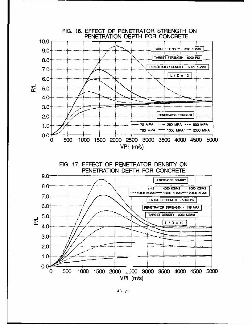
FIG. 16. EFFECT OF PENETRATOR STRENGTH ONPENETRATION DEPTH FOR CONCRETE
10.0-
9.0- .......... I....... .......... TARGET7 DENSITY -2200 KG 3 ....
8.0- / ~~TARGET STRENGTH-500SI
70 PENETRATOR DENSITY- 17120 KCM1
3.0 ....... ..........6 . .............
L 5.0 -5 ------------- 2-00----
9.0 ...................... .......
8.0
70- 2000 ~M3- 16000 KGM3.**-20000 KGM3
0.0
0 500 1000 1500 2000 2.500 3000 3500 4000 4500 5ý000VPI (m/s)
FIG 17 EFEC OFPEETRTORDESIT20

Resolution Enhancement of Passive Millimeter-wave Imaging
Zhi DigAssistant Professor
Department of Electrical EngieeringAuburn UniversityAuburn, AL 36849
(205)-844-1817
Final Report forSummer Faculty Research Program
Wright Laboratory/MNGSEglin Air Force Base, FL 32542-5434
Sponsored by: Air Force Office of Scientific ResearchBolling Air Force Base, Washington, D.C.
August 1993
44-1

Resolution Enhancement of Passive Millimeter-wave Imalin
Zhi DingAssis-,ut Professor
Department oi •.ctrical EngineeringAuburn Univsity
Abstract
Although passive millimeter-wave imaging is capable of operating under adverse conditions andprovides the advantage of stealth, its poor resolution severely limits its applicability in practice.The problem of resolution improvement for a passive millimeter-wave imading system is investi-gated. The feasibility of significant image resolution improvement is studied. A new differentiation-integration deconvolution (DID) algorithm is proposed for resolution improvement on images con-taining extended targets and is tested through extensive simulations. A criterion for measur:super-resolution is also presented and shows that our proposed DID algorithm improves the reso-lution of test images by 2-3 times.
44-2

Resolution Enhancement of Passive Miimeter-wave Imaging
Zhi Ding
1 Introduction
This report describes the problem of resolution enhancement for passive millimeter-wavedevices and summarizes our recent results in this area supported by the AFOSR Summer FacultyResearch Program.
Compared with infra-red, millimeter-wave (MMW) encounters less obstruction through fog,dust, smoke, and artificial cover. The use of passive MMW imagng in air surveillance, targetseeking, and civilian applications such a vehicle guidance offers a viable alternative to infrared(IR) imaging under such adverse conditions. Passive imaging is particularly attractive to militaryoperations and intelligence gathering since a passive sensor emits no signal and therefore offersstealth. Unlike IR, sensors that are incapable of detecting targets under cover or in foggy anddusty conditions, MMW sensors can provide adequate information in these unfavorable situations.Moreover, the use of passive millimeter-wave imaging, together with IE. imaging, can improveand enhance target recognition capability and visual images. Additionally, MWI sensors areexpected to be employed in many ground-based, airborne, and spaceborne applications such asautonomous aircraft landing and collision avoidance. Recent experiments by TRW [11 providesome very encouraging results.
Over the years, the wide application of IMW imaging is hindered by the hardware limitationin constructing high gain, low noise receivers. Fortunately, the technological advancement in mi-croelectronics has drastically improve the performance of MMW receiver. Nevertheless, a morecritical obstacle still exists which will require important breakthrough, namely, the improvement ofpoor angular resolution at MMW frequencies. This summer research project centers on the issueof resolution improvement based on the use of advanced digital signal processing of the receivedimage signals.
In this report, the low resolution problem of passive millmeter-wave imaging is outlined insection 2. Next various existing approaches to this well-known problem are summarized withrespect to their advantages and disadvantages in section 3. Our new algorithm is presented insection 4 and the issue of superresolution is discussed in detail. Simulation results of our approachcompared with some existing methods are presented in section 5. Finally, a summary of this reportis given in section 6.
2 Problem Statement: Diffraction Limit on Angular Resolution
Passive MMW imaging data can be collected from a single MMW sensor (antenna) by scanning a2-dimensional scene. Alternatively, a line array or a 2-D focal-plane array can also be applied toachieve quicker and more efficient data acquisition. Nevertheless, the angular resolution of a single
44-3

sensor or an array of sensors will be dictated by the Rayleigh diffraction limit, i.e.,
0 2Z -5 (2.1)
where )\ is the millimeter wavelength and D is the aperture size of the antenna (sensor).
The diffraction severely limits the image resolution of passive MMW devices. For example, at the
frequency of 94GHz, an antenna with one foot diameter has an angular resolution of approximately
0.60. At a distance of 1 kin, this translates to a target resolution of merely 10.6 meters. Such a
poor resolution may be barely sufficient to identify large objects such as ships and buildings. For
many practical purposes, the antenna size is limited, making it impossible to simply increase the
physical aperture of the sensors to gain high image res,,±uton. Thus, in order for passive MMW
imaging to become widely applicable, its angular resolution must be significantly improved with
the aid of advanced and specialized signal processing systems.
3 The Critical Issue of Image Resolution Enhancement
The low angular resolution of the passive MMW sensors due to the longer wavelength is the primary
obstacle to its deployment in many military and civilian applications. Our proposed research isaimed at developing post-detection signal processing methods to significantly improve the image
resolution. Our objective is to design effective solution to sharpen the received radio image based
on the knowledge of the antenna beampattern.
3.1 Millimeter-wave Imaging
For the simplicity of representation, we consider the problem of resolution improvement for 1-D
images. It is evident that the 2-D problem is simply a straightforward generalization of the 1-Dcase.
Denote the antenna beampattern as h(4) where 6 is the angle of signal arrival. The receivedpassive image at the sensor after scanning a 1-D scene z(O) can be written as
y(O) = h(O) ® x(O),
where z(O) is the true original image, h(o) the point spread function (PSF) of the sensor (antenna),
and y(o) is the received image. The noncoherent antenna beampattern h(o) operates as a blurring
function to the actual signal z(O). In practice, the received signals are sampled to generate the
following relationship,
yl, = hA ® zk. (3.1)
Thus, recovering the source signal zk based on yA, and hk becomes the standard deconvolution
problem. It should be noted that all signals z,,, yA:, and hA: in passive imaging are positive since the
passive imaging system only forms an image of intensity irrespective of the phase. This positivity
condition is in fact crucial to solving the image deconvolution problem.
The deconvolution problem has been extensively studied in the past, and image processingtextbooks often contain various image restoration treatments. It has been long recognized that the
44-4

deconvolution problem is ill-posed when the bandwidth of the point spread function hk is limited
and when additive noise n1 is present in the received image:
yk = hk @ Zjx + nk. (3.2)
The PSF hA. is typically lowpass in nature. As a result, all the high spatial frequency content
of Xk will be attenuated by hk and thus, high frequency (high resolution) information is eitherirretrievably lost in yk or highly attenuated. In order to regain the attenuated high frequencycontent, an inverse filter (high-pass) needs to be used on the received image, which will have the
undesirable noise amplification effect.
The ill-posed-ness of this problem arises from the conflict between the need to recover the lost
high frequency information and the necessity to suppress high frequency additive noise at the same
time. It is essential that the original image be recovered as precisely as possible without severely
amplifying the receiver noise. Hence the optimum solution lies between the inverse filter and anideal lowpass filter to suppress the additive noise. Wiener filtering and regularization are typical
balanced solutions to accomplish such conflicting tasks.
3.2 Summary of Existing Works
Essentially, the problem of millimeter-wave image resolution enhancement is not different from thetraditional image restoration problem that has been studied for years. Although many methods
have been proposed and studied in the past, the image deconvolution problem is still a difficultand open problem. Achieved resolution improvement has been modest for the most part. Two
basic kinds of approaches dominate the literature: linear and nonlinear deconvolutions. We now
summarize their major advantages and weaknesses when applied to the millimeter-wave resolutionimprovement problem.
3.2.1 Linear Deconvolution
The linear deconvolution methods accomplish the task of resolution enhancement by applying a
linear filter (or transformation) on the received image. The purpose of this filter is to suppressnoise while recovering the attenuated high frequency content of the image. Various existing linear
deconvolution methods typically belong to one the following categories:
"* Inverse Filtering [8, 14];
"* Singular Value Decomposition (SVD) [71;
"* Wiener Filtering (Minimum Mean Square Error) [8];
"* Regularization [9, 10, 12, 15].
In inverse filtering, the objective is to recover the original image by reversing the lowpass effect
of the PSF. It in effect searches for a least square solution of the convolution equation. Althoughvery simple, the inverse filtering approach normally produces poor result due to its amplification
44-5

of receiver noises. The SVD approach is an effective alternative to inverse filtering, It attempts toapproximate the inverse filter without excessive noise amplification.
Wiener filter is another way to avoid noise amplification. By minimizing the mean square er-ror between the recovered image and the original 'mage, Wiener filter provides a good balancebetween image restoration and noise suppression. -z :.•;ization was an useful tool developed by
Tikhonov [91 to solve general ill-posed problems. objective is to deconvolve the image whilemaintaining certain degree of smoothness on the aeconvolved image. Among numerous regular-ization methods, Reynold attempted to find an optimum regularization coefficient, while Gleedconstructed a two-step regularization approach.
The major advantage of various linear deconvolution methods is that they are always verysimple in concept and implementation. In fact, all of the linear algorithms are data independentand only require a one-step filtering or matrix operation on the received image. Thus, they arehighly desirable onboard a seeker where the computational power is rather limited. Unfortunately,linear deconvolution methods can only reshape the nonzero spectrum of the received data. It cannotextrapolate or recover any lost frequency content. Hence, linear deconvolution can only achievevery modest resolution improvement. With the exception of inverse filtering that often generatesnoisy images, the recovered image tends to be smooth and the finer details of the image, such assharp edges, are often suppressed.
3.2.2 Nonlinear Deconvolution
In order to recover any spectral content that has been complete filtered out by the antenna PSF,frequency domain extrapolation is necessary. Since linear methods are incapable of extrapolatingin frequency domain, only nonlinear methods can more effectively increase the image bandwidthand improve the image resolution. However, this advantage can sometimes be offset by higher realtime computation requirement due to their data dependency.
The basis of any nonlinear deconvolution algorithm is the use of prior knowledges with regardto the original image. In passive imaging system, the received and the orignal image data are allpositive and bounded. In addition, the original image may only have a finite (known) spectral orspatial support. By constraining the deconvolved image to satisfy these known conditions of theoriginal image, nonliner operations are used to assure the positivity and the finite support of therecovered image. Nonlinear operations are able to extend the image bandwidth and hence improvethe image resolution.
The following nonlinear deconvolution algorithms are well known and commonly refereed to:
"* Jansson-van Cittert method [6];
"* Schell and Biraud method [6, 14];
"* Maximum entropy deconvolution [14, 17, 18];
"* Constrained iterative deconvolution (CID) method [11].
44-6
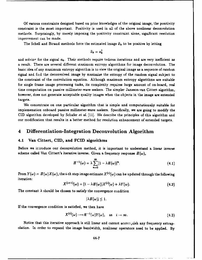
Of various constraints designed based on prior knowledges of the original image, the positivityconstraint is the most important. Positivity is used in all of the above nonlinear deconvolutionmethods. Surprisingly, by merely imposing the positivity constraint alone, significant resolutionimprovement can be made.
The Schell and Biraud methods force the estimated image 4 to be positive by letting
Xk 2
and solving, for the signal at. Their methods require tedious iterations and are very inefficient asa result. There are several different maximum entropy algorithms for image deconvolution. Thebasic idea of any maximum entropy algorithm is to view the original image as a sequence of randomsignal and find the deconvolved image by maximize the entropy of the random signal subject tothe constraint of the convolution equation. Although maximum entropy algorithms are suitablefor single frame image processing tasks, its complexity requires large amount of on-board, realtime computation on passive millimeter-wave seekers. The simpler Jansson-van Cittert algorithm,however, does not generate acceptable quality images when the objects in the image are extendedtargets.
We concentrate on one particular algorithm that is simple and computationally suitable forimplemenation onboard passive millimeter-wave seekers. Specifically, we are going to modify theCID algorithm developed by Schafer et aL. [11]. We describe the principles of this algorithm andour modification that results in a better method for resolution enhancement of extended targets.
4 Differentiation-Integration Deconvolution Algorithm
4.1 Van Cittert, CID, and FCID algorithms
Before we irtroduce our deconvolution method, it is important to understand a linear inversescheme called Van Cittert's iterative inverse. Given a frequency response H(w),
H-1 (w) = A '[I - AH(w)Jn. (4.1)n=O
From Y(w) = H(w)X(w), the i-th step image estimate X(')(w) can be updated through the followingiteration:
X('+1 )(w) = [1 - AH(w)]X(0(w) + AY(w). (4.2)
The constant A should be chosen to satisfy the convergence condition
IAH(w)I < 1.
If the convergence condition is satisfied, we then have
X(')(w) --H-(w)Y(w), as i -, oo. (4.3)
Notice that this iterative approach is still linear and cannot accorzyiish any frequency extrap-olation. In order to expand the image bandwidth, nonlinear operators need to be applied. By
44-7
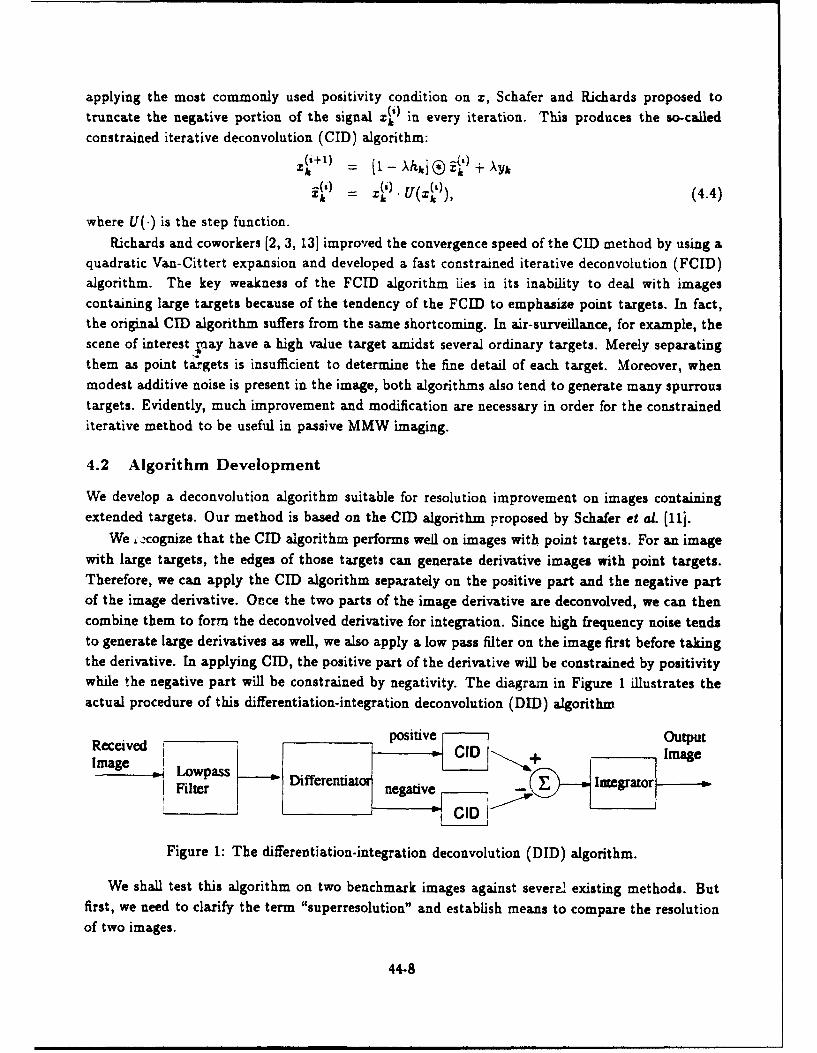
applying the most commonly used positivity condition on z, Schafer and Richards proposed to
truncate the negative portion of the signal z3 in every iteration. This produces the so-calledconstrained iterative deconvolution (CID) algorithm:
Z1 [1-A_ i)+A,1) - -'÷
i) . U(4)), (4.4)
where U(.) is the step function.
Richards and coworkers [2, 3, 131 improved the convergence speed of the CID method by using aquadratic Van-Cittert expansion and developed a fast constrained iterative deconvolution (FCID)algorithm. The key weakness of the FCID algorithm lies in its inability to deal with imagescontaining large targets because of the tendency of the FCID to emphasize point targets. In fact,the original CID algorithm suffers from the same shortcoming. In air-surveillance, for example, thescene of interest ptaay have a high value target amidst several ordinary targets. Merely separatingthem as point targets is insufficient to determine the fine detail of each target. Moreover, whenmodest additive noise is present in the image, both algorithms also tend to generate many spurroustargets. Evidently, much improvement and modification are necessary in order for the constrainediterative method to be useful in passive MMW imaging.
4.2 Algorithm Development
We develop a deconvolution algorithm suitable for resolution improvement on images containingextended targets. Our method is based on the CID algorithm proposed by Schafer et at. [11].
We xcognize that the CID algorithm performs well on images with point targets. For an imagewith large targets, the edges of those targets can generate derivative images with point targets.Therefore, we can apply the CID algorithm separately on the positive part and the negative partof the image derivative. Occe the two parts of the image derivative are deconvolved, we can thencombine them to form the deconvolved derivative for integration. Since high frequency noise tendsto generate large derivatives as well, we also apply a low pass filter on the image first before takingthe derivative. In applying CID, the positive part of the derivative will be constrained by positivitywhile the negative part will be constrained by negativity. The diagram in Figure 1 illustrates theactual procedure of this differentiation-integration deconvolution (DID) algorithm
Receivedpositive Output
Image Lowpass Di lfeenaor
Filter Differentiat negative IID t•
Figure 1: The differentiation-integration deconvolution (DID) algorithm.
We shall test this algorithm on two benchmark images against severa2 existing methods. Butfirst, we need to clarify the term "superresolution" and establish means to compare the resolutionof two images.
44-8

4.3 On Superresolution
The term superresolution is an often encountered term in the literature of array signal processingas well as in image restoration. Unfortunately, this term is often misused due to its favorableconnotation. The misuse of superresolution has created a lot of confusion in the area of image
deconvolution. Sometimes outragous claims of resolution improvement are made due to misunder-standings. In this section, we attempt to clarify this confusion and explain how we propose tomeasure the resolution improvement of any given image restoration method.
Superresolution often refers to the ability to resolve two point targets that are separated byless than the Rayleigh diffraction limit. It is typically demonstrated by showing the ability of analgorithm to locate the positions of two point targets that are so close together that they cannot be
separated in the original image. In this sense, superresolution in image processing is not different
from superresolution in the direction finding problem in array processing. In both cases, only pointtargets are of concern and the objective is merely to locate the positions of those point targets.
The possible distortion on the shape or the intensity of the image is often of no concern.
In the passive millimeter-wave seeker problem, we not only need to locate the targets but alsoto properly identify targets in the image. Therefore, we need to improve resolution on both pointtargets and extended large targets. Although many "superresolution" methods claim to be capable
of achieving resolution improvement by 10 times, in reality, their claims are based on separatingtwo closeby point targets. When applied to extended targets, these algorithms typically either failto function properly or provide very modest improvement on resolution. Clearly, the difficulty in
dealing with extended targets is the key disadvantage of many existing nonlinear deconvolution
methods.
Another key difficulty in dealing with extended targets lies in the very definition of superreso-lution. Because of the nature of the image containing extended target, Rayleigh diffraction limit
can no longer be used in defining resolution. Given two images of the same scene, there is noquantatative meaure to compare the resolution of the two images without visual inspection. Asa result, it is difficult to determine how much resolution improvement has been made by a given
deconvolution method.In order to measure objectively the actual amount of resolution improvement, we need to return
to the initial definition of angular resolution in terms of the antenna size. To improve the resolutionby a factor of two, the antenna diameter needs to increase to twice its original length. The antenna
needs to be four times as large to achieve four times resolution improvement, and so on.
Definition:
Let y1, be the image formed from xk using antenna n times larger. The deconvolved image it
has resolution improvement of n times if
mrin II,;, - iI2 = -Iy _i1 2 < 0.111_A:11, (4.5)I
In other words, a resolution improvement of n times is accomplished if the deconvolved image
44-9

4 is closest to the image y' formed by increasing the antenna size n times and the difference
between the two images is smaller than 10% of the true image energy. While the difference betweenthe two images is obviously a good choice for judging resolution improvement, the upper boundmust be present to avoid pathelogical cases when 4 bears no resemblance to the true image but is
relatively closer to y*.
Our definition of resolution improvement is intuitive and can easily be measured in practice.
If the deconvolved image is very similar to the image received by an antenna n times larger, thencertainly the angular resolution is improved by n times. Here, not only we have to separate twopoint targets, the fine details of the original image also need to be preserved.
5 Test Examples
5.1 Test Setups
Two benchmark images are used in testing the DID method. The objects in the images are designedto resemble extended targets. They are constructed to contain distinctly sharp edges and to spana large area in the image. Figure 2(a) and (b) show the two benchmark images used in our tests.
The antenna point spread function is chosen to be a sinc-squared function as shown in Figure 2(c)whose lowpass frequency response is shown in Figure 2(d)
For the both images, we apply the DID algorithm under different clutter and noise levels.The clutter and the additive noise are generated independently by squaring Gaussian noises. Thelowpass filter in the DID algorithm was chosen to be nearly ideal and have the same passband asthe PSF frequency response. In all our simulations, A = 0.1 was also selected and 100 iterations
were run for each image.
5.2 Test Results on Image A
For image A, we first apply our algorithm to the noiseless received image. No clutter was added inthe original image. Figure 3 shows the received image and the deconvolved image. We then added
random and independent clutters to the original image so that the signal to clutter ratio (SCR) is10dB. 10 independent clutter patterns were simulationed and the 10 deconvolved images are shownin Figure 3 together with the received image. Satisfactory image recovery was achieved.
We then increase the noise level so that SNR=30dB and 20dB, respectively. 10 independentsimulation runs were completed for the two noise levels and the recovered images are shown togetherwith the noisy received images in Figure 4 and Figure 5, respectively. Under reasonable amountof noise level (SNR=30dB), the DID algorithm performs very well for this test image. Most of thedetails are recovered in the deconvolved image.
5.3 Test Results on Image B
For image B, we also apply our algorithm to the noiseless received image. Figure 6 shows the
received clutterless image and the deconvolved image. We then added random and independent
44-10

3 (a). Image A (b). Image B
2- j 2- -l
0' 010 50 100 0 50 100
samples samples
0.08, (c). Antenna PSF I (d). PSF frequency response
o.06 4 0.8 ,0.06 ,
0.042 -i 0 -
0.4
I / s0.'
-50 0 50 -50 0 50
Figure 2: Two test images for resolution improvement.
clutters to the original image so that the signal to clutter ratio (SCR) is 10dB. 10 independentclutter patterns were simulationed and the 10 deconvolved images are shown in Figure 6 togetherwith the received image. Satisfactory image recovery was achieved.
We then increase the noise level so that SNR=30dB and 20dB, respectively. 10 independentsimulation runs were completed for the two noise levels and the recovered images are shown togetherwith the noisy received images in Figure 7 and Figure 8, respectively. Under reasonable amountof noise level (SNR=30dB), the DID algorithm is also successful in deconvolving image B andrecovered most of the details in the deconvolved image.
44-11
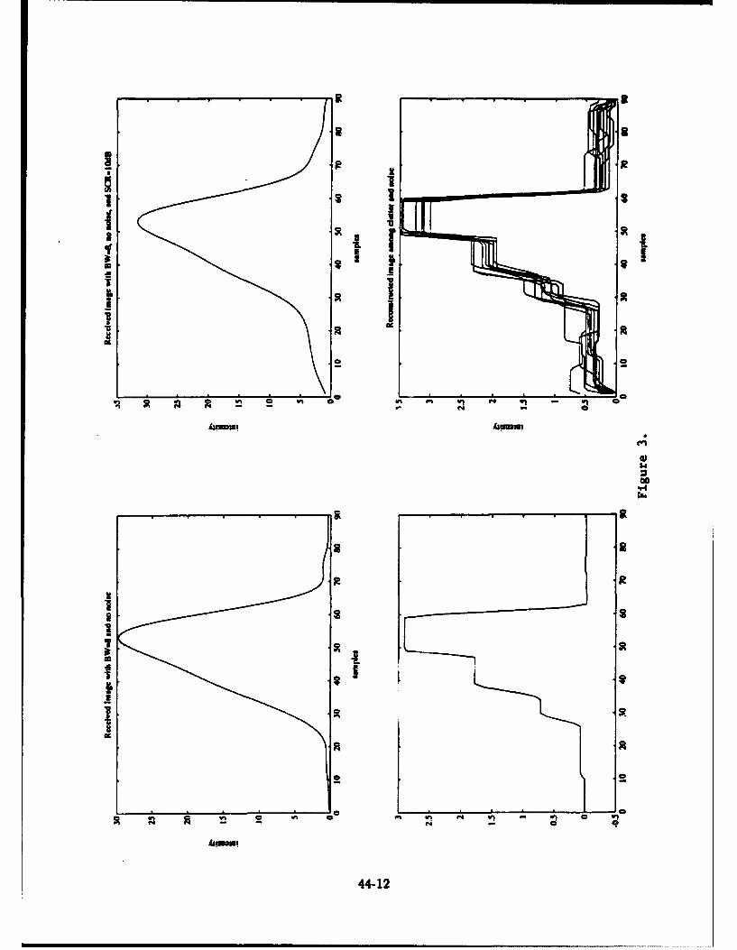
8 3
3 3
U
2
*11 1
U81 "U
* II
I a I a
I IA a
0
e
e
A3.mu1
'.4El
"'.4
Ia�
a -a
a a
U*1a S SII a. a4**1 SI SIa
I aj a
C
- a
Aainaui
44-12
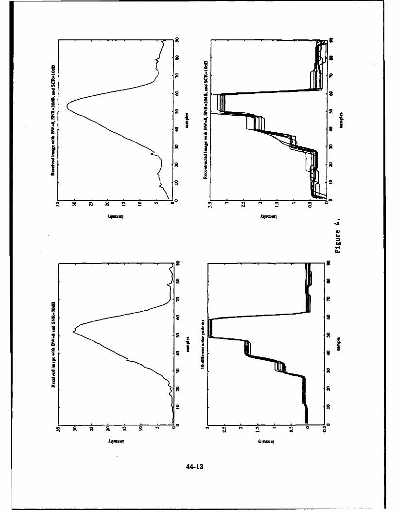
al
a IL
0 a0
44-1

A 2
i. I
i st
44-14

8 1
% In In I
neir
U 8
- SoU II .1
r4.
44-15
i nmmm mm• • mmn mm0

- : I a
I U
1
V..! C•
S -1

a .18£ I
Ma iI-
I2 2
2- I .3
I*�I
U
* U
2 * 2* I
U 2
2 2
a j 0
o 0v� �I 2 � 2 0 - W� C
- a
CamE
a)I.'
94�Zd
3 8
2 2
a2 2
S SI I
S
£ 2.3.
I 3 I1 2� I* IU U
2 2II *1
2 2
o 0
C� 2 Vb 0 � C - C
44-17

5.4 Synopsis
We summarize our test results by estimating the normalized mean square errors between the trueclutterless image and the deconvolved image under different noise levels. We would like to determine
the amount of resolution improvement attained by the DID algorithm in our simulation. To achieve
accurate measurement, we perform 100 independent simulations for each simulation setup.
Figure 9 demonstrates the effect of the noise and clutter on the deconvolution of the two test
images. Clearly, as the noise increases, the NMSE tends to increase rapidly. For SNR=lOdB, thedeconvolution method fails to recover the original image as the NMSE is over 30%.
100 (a). NMSE for Image A 100 (b). NMSE for Image B
- " q F-SCR=OdBSCR=lOdB SR"d
10"| -- - No clutter 10"L-- _ _-_ '--.. No clutter
10-21 10-210 20 30 inf 10 20 30 inf
SNR in dB
0.07 (c). Resolution of Imae A 035[ (d). Resolution of Image B
0.06- 0.035
Q 0.05 -\ zJ 0.03
Z 0.04 z 0.025
0.03 0.02-
0.02 0.0151 2 3 4 8 1 2 3 4 8
3 dB PSF beamwidth 3 dB PSF beamwidth
Figure 9: Resolution improvement on Images A and B using DID method.
We reduce the beamwidth of the antenna PSF to simulate the effect of antenna size increase.
The original beamwidth of 8 was reduced to 4, 3, 2, and finally 1, representing the antenna sizeincrease by factors of 2, 8/3, 4, and 8, respectively. The images are clutterless and the receiver SNRis 30dB. Simulation results are shown in Figure 9(c) and 9(d). From Figure 9(c), we can determinethat the resolution of the deconvolved Image A has been increased 3 times. From Figure 9(d),
resolution of the deconvolved Image B is increased by a factor of 2. Based on these !.Imulations, we
44-18

conclude that the DID method is capable of improving image resolution by 2 to 3 times.
6 Concluding Remarks
The research work performed during the AFOSR. Summer Research program is aimed at enhancingthe resolution of passive milfimeter-wave imaging devices. While millimeter-wave detection offers
certain advantage over IR in its easy penetration through fog, dust, smoke, and artificial cover, its
poorer angular resolution poses a critical obstacle to its wide application in military and civilianenvironment. Our research in improving angular resolution based on the design of new image
deconvolution techniques significantly improved the performance of MMW imaging. In order to
make it possible for a receiver with small antenna to achieve imaging resolution comparable to the
traditional IR imaging, further resolution improvement is crucial to both the military and civilian
applications of passive MMW imaging systems.
Acknowledgement
The author wishes to thank his MNGS host, Mr. Bryce Sundstrom, for providing excellent technicalsupport and for many helpful discussions throughout this project.
References
[1] S. K. Young, R. A. Davidheiser, B. Hauss, P. S. C. Lee, M. Mussetto, M. M. Shoucri, and
L. Yujin, "Passive millimeter-wave imaging", Quest, TRW Space & Defense Sector, Vol-13,
No. 2:3-20, Winter 1990/1991.
[2] Mark A. Rtichards, "Iterative Noncoherent Angular Superresolution", In Proc. 1988 IEEE
National Radar Conf., pages 100-105, Ann Arbor, MI, 1988.
[3] M. A. Richards, C. E. Morris, and M. H. Hayes, "Iterative Enhancement of Noncoherent Radar
Data", In Proc. 1986 IEEE Int. Conf. on Acoustics, Speech, and Signal Processing, pages
1929-1932, 1986.
[4] M. A. Richards, "Iterative Deconvolution in Noncoherent Radar Data, In Proc. 1985 IEEEInt. Conf. on Acoustics, Speech, and Signal Processing, pages 434-437, 1985.
[5] E. D'Anna and M. A. Richards, "Superresolutione, In Proc. Workshop on Detection, Discrim-ination, and Classification of Targets in Clutter, Huntsville, Alabama, November 1990.
[6] Peter A. Jansson, "Modern Constrained Nonlinear Methods", In Deconvolution with Applica-tions in Spectroscopy.,, Peter A. Jansson, ed. Academic Press, Orlando, FL.
[7] T. S. Huang (ed.), Picture Processing and Digital Filtering, Springer-Verlag, 1975.
[8] Anil K. Jain, Fundamentals of Digital Image Processing Prentice Hall, 1989.
44-19
[9] A.N. Tikhonov, "Solution of Incorrectly Formulated Problems and the Regulariation Method",Sovnet Math. Dokl., vol.4, pp. 1035-1038, 1963.
[10] V.A. Morozov, Methods for Solving Incorrectly Posed Problems, Springer-Verlag, 1984.
[11] R.W. Schafer, R.M. Mersereau, and M.A. Richards, "Constrained Iterative Restoration Algo-rithm", Proceedings of the IEEE, vol.69, no.4, pp. 432-450, April 1981.
[121 J.W. Hilgers and W.R. Reynolds, "Instabilities in the Optimal Regularization Parameterrelating to Image Recovery Problems," Journal of Opt.Soc.Am.A, vol.9, pp. 1273-1279, August1992.
[131 M.A. Richards, C.F. Barnes, C.L.Belcher, and B.M. Keel, "Super Resolution in Low Signal-to-Clutter Ratios for Millimeter Wave Seekers," Final Report AFATL-TR-90-62, Air ForceArmament Laboratory, Eglin AFB, September 1990.
[14] B.R. Frieden, "Image Enhancement and Restoration", In Picture Processing and DigitalFiltering, T. S. Huang, ed., Springer-Verlag, 1975.
[15] D.G. Gleed and A. H. Lettington, "Application of Superresolution Techniques to PassiveMillimeter-wave images", Unpublished Report, Royal Signals and Radar Establishment, GtMalvern, Worcs, UK, 1991.
[16] R. Appleby and A.H. Lettington, "Passive Millimeter Wave Imaging", Electronics and Com-munications Engineering Journal, vol.3, no.1, pp.13-16, 1991.
[17] X. Zhuang, E ,Ostevold, and R.M. Haralick, "A Differential Equation Approach to Mani-mum Entropy Image Reconstruction", IEEE Transactions on Acoustics, Speech, and SignalProcessing, vol.35, no.2, pp. 208-218, February 1987.
[18] S.F. Gull and J. Skilling, "Maximum Entropy Method in Image Processing", IEE Proceedings,Part F, vol.131, no.6, pp. 646-659, Oct.1984.
44-20

Field-Induced Atomic-Scale Manipulation of Semiconductor,
Metal, and Conductive Polymer Surfaces with a STM
Simon Y. Foo
Assistant Professor
Department of Electrical Engineering
Florida State University
Tallahassee, FL 32306
Final Report for:
Summer Faculty Research ProgramWright Laboratory
Sponsored by:
Air Force Office of Scientific Research
Boiling Air Force Base, Washington, DC
July 1993
45-1

Field-Induced Atomic-Scale Manipulation of Semiconductor,
Metal, and Conductive Polymer Surfaces with a STM
Simon Y. Foo
Assistant ProfessorDepartment of Electrical Engineering
Florida State University
Abstract
The goal of our experiments is to demonstrate the ability to "etch" very fin' grooves
(a few angstroms in width and depth) on semiconductor, metal, and conductive polymer
surfaces using a scanning tunneling microscope (STM). Specifically, our specimensconsist of n-type and p-type <I I I> silicon, gallium-arsenide, gold, and polypyrrol, with
air and water being the electrolytes. The motivation behind this work is the theory of field-induced evaporation of surface atoms, i.e., atoms can be removed if an appropriatelyvoltage-biased STM tip is brought close to a conducting surface. A "C" program drives theSTM tip to a specific location on the surface to be etched making a groove or a ditch.
Grooves traced out in a fractal pattern are expected to provide high surface area electrodesnecessary to achieve high capacitance. This research may eventually lead to the fabrication
of ultra-high-speed quantum devices as well as high capacitance electrodes for high energy
density capacitors.
45-2

Field-Induced Atomic-Scale Manipulation of Semiconductor,
Metal, and Conductive Polymer Surfaces with a STM
Simon Y. Foo
The ability to "see" beyond the capabilities of our eyes has always been fascinating
and challenging. Typically our human eye has a resolution of about 100 lim, limited byrods and cones in the reina. The more powerful optical microscope has a maximum
magnification of 1000X over human eye (i.e., about 0.1 to 0.2 gm resolution), limitedonly by the diffraction of light. In contrast, the scanning electron microscope (SEM) has amaximum resolution of 50 to 100 A, limited by the focus of the electron beam. The recentinvention of the scanning tunneling microscope (STM) in 1982 gave us the ability to see ineven more details - right down to the atoms! The STM is capable of imaging the atomicstructure of conductive surfaces with an incredible resolution of 1 to 3 A, limited only bythe sharpness of the tip (ideally one atom at the end of tip!). The drawback of the STM isthat the sample under observation has to be conductive in order for electron tunneling to
occur.
Surprisingly, the STM, which was invented by Binnig and Rohrer [1], is useful notonly to "observe" atoms but also to "manipulate" atoms of semiconductor surfaces. Thefirst demonstration of the latter was done by Becker et al. [21, where atomic-scaleprotrusions on Ge <111> surface were made by increasing the bias of a W tip under
constant tunneling current. Since then, there has been considerable interest in using thescanning tunneling microscope (STM) to modify the surface topography of semiconductorsat nanometer-scale (see [3] -[7]). Manipulation of semiconductor surfaces is of particularinterest for the fabrication of ultra-high-speed quantum devices and high energy capacitors.
Field-Induced Evaporation of Surface Atoms
Lyo and Avouris [5] and Kobayashi et al. [7] have shown that if a STM tip, biasedwith either a positive or a negative voltage, is placed close to a Si <111> surface, Si atomsare removed from the surface, i.e., a hole is created on the surface. Grooves or ditches canbe created by scanning the tip parallel to the surface. The diameter of the hole and the widthof the ditch can be controlled by changing the magnitude of the tip bias and the duration ofscan. Specifically, the amount of Si atoms removed from surface depends on experimentalparameters such as polarity, magnitude, duration of bias voltage applied to the tip, the elec-
45-3

tron tunneling current between the tip and the surface, and the material of the tip [7].
The result can be explained in terms of field-induced emission of ions from the Si
sample. If we apply an appropriate positive (/negative) voltage to the STM tip, a strong
positive (/negative) field is created at the Si surface. This strong field ionizes Si atoms at the
surface into negative (/positive) ions and pulls them apart from the surface, i.e., Si atoms at
the surface evaporate as negative or positive ions, depending on the polarity of the tip
voltage.
The Burleigh Instructional STM
The STM system used in our experiments is a low-cost Burleigh Instructional STM
system, as shown in Figure 1. Basically, the system consists of the Mechanical Head,
Control Electronics, data acquisition card, and a computer. The sample to be examined or
etched is mounted inside the Mechanical Head cavity, as shown in Figure l(b). The tip
which is typically made of either tungsten (W) or Platinium Iridium (PtIr) is held
magnetically by a piezoelectric (PZT) ceramic. The bending and elongation of the PZT
under appropriate high voltage are responsible for the scanning and terrain-following
actions of the STM. A general idea of how the STM works is shown in Figure 2. In a
constant-current mode, a constant tunneling current is maintained through the Negative
Feedback Control Electronics as the PZT tip scans across a surface. The negative feedback
can be adjusted by the Servo Loop Response controls (Figure 2(b)), which are used to
optimize the PZT-Z motion when scanning a particular sample terrain. Basically the Time
Constant and Gain controls determines how fast and how much to adjust the Z position,
respectively, while the Filter acts as a low-pass filter. That is, if the Time Constant is set to
minimum, the servo loop will respond to any variations in the terrain very quickly. If the
Gain is set high, the servo loop response to any tunneling current variation will be very
large. If the Filter is set high, all high-frequency signals in the tunneling current will be
filtered out. In all our imaging experiments, Time Constant is set to maximum
(compensated by slower scanning rate of 0.5 ms/sample), Gain set to minimum (to avoid
oscillations), and Filter set to maximum. A tip bias voltage of 0.05V and reference current
of 2 nA are used. For more accurate results, the STM should be placed in a ultra-high-
vacuum (UHV) chamber to avoid electron scattering and adsorption by reactive gases in the
air. Otherwise dust particles or gases present in the air between the tip and the sample may
form an undesired conducting path thereby distorting the true image. Typically a chamber
pressure of 1E-8 to 1E-10 Torr is considered UJHV.
45-4

The initial experiment to demonstrate the theory of field-induced evaporation of
surface atoms is to simply position the STM tip at the center of scanning area, apply a
constant -10V bias to the tip for about 60 seconds, and then observe the groove made (if
any) by imaging the whole area using a small +0.05V tip bias. The specimens for our
experiments consist of n-type <li1> and p-type <111 > silicon, gallium-arsenide, gold,
and polypyrrol, a conductive polymer with a high surface area, as shown in Figure 3.
The major variables which influence the quality of STM work are tip preparation
and vibration isolation. Tip preparation is very important in getting good atomic-scale
images of surfaces. In order to achieve the atomic resolution capabilities of the STM, the
probe must be sharpened to a tip such that it has only one atom at the tip end (ideally!).
This atom is primarily responsible for the current tunneling between the tip and the
conductive sample. There are two preferred tip materials for STM work, namely W and
PtIr wires. PtIr wires are quite expensive but soft enough to be cut diagonally into a sharp
tip using a metal cutter. In contrast, W wires are cheaper, alot harder, and will ruin most
cutters. The preferred method is to electrochemically etched the W wire into a very sharp
tip. Both PtIr and W tips are can electrochemically etched using an adjustable AC
autotransformer (also called Variac or Powerstat), as shown in Figure 4(a)-(b). It is also
possible to etch W wire using a constant DC power supply, as shown in Figure 4(c)-(d). In
both cases, the anode is the W or PtIr wire while the cathode can be a simple copper wire.
The etching solution used is a 5 molar potassium hydroxide (KOH) solution. Figure 5
shows the SEM pictures of a not-so-sharp PtIr tip (cut using a pair of cutters) and a very
sharp electrochemically etched W tip. Note that tips with long "wiskers" are very
susceptible to acoustic vibrations, and therefore they are unsuitable for STM work.
When the STM is used in a constant tunneling current mode, it is required that the
tip and the sample surface be only 10 A apart at all times without crashing the tip onto the
surface and distorting the true image of the surface profile. Therefore, it is extremely
important that any vibrations due to walking around the room, air conditioning fan
blowing, etc., be eliminated as much as possible. There are basically three methods for
isolating the STM from these vibrations, as shown in Figure 6. Historically, the first
method of vibration isolation used was the superconducting levitation or the Meissner
Effect. The STM is placed on an array of magnets levitated above a superconductor chilled
by liquid nitrogen. Alternatively, a simple vibration isolation method is to hang the STM by
elastic springs from a fixed point. Any small vibrations to the plate holding the STM head
is absorbed by the springs. Yet another way is to place the STM on top of a series of metal
plates, stacked on top of each other and separated by "0" rings (elastomer spacers). These
45-5

spacers act as springs and dampers.
The initial experiments were first performed under normal room conditions, i.e.,with air as the etching medium. The samples were first imaged using a +0.05V bias with aconstant 2 nA tunneling current, before a large bias of -10V is applied to the tip. After 60seconds elapse, the same spot is imaged again to observe the effect if any. Figure 7 showsthe STM image (30A by 30A) of low and high-surface area polypyrrol. Dark spacesbetween surface atoms are due to the fact that atoms beneath the surface atoms are about 3A away, with an extremely small probability of electron tunneling. Other dark areas are dueto atoms with less energetic electrons and non-conductive contaminants. Figure 8(a)shows the diamond-shape arrangement of the n-type Si atoms in the <I 1>-plane; Figure8(b) shows gold-coated p-type <I 11> Si; Figure 9(a), gold-coated GaAs; and Figure 9(b),defects in polycystalline GaAs. However, we were unable to observe any "ditches" createdby the evaporation of surface atoms under normal room conditions.
We then proceed to using water as the etching medium since hydrogen atoms arehighly reactive. A teflon "tub" has to be specially built to accomodate the sample and thewater. This tub sits on top of the sample carriage, and is carefully inserted into the STM
Head cavity. Figure 10 shows the setup of the experiment.
2 rail gold wire part of specimen withgold surface contact specimen with goldgold wire clamped coat underneath
by specimen
to G teflon tubIfilled withwater to GND
4-40 plastic screws to hold specimen
(a) (b)
Figure 10. (a) An elegant setup to electrochemically "etch" a specimen using the STM.
(b) A crude but workable alternative.
45-6
A -10V bias is apply at the tip for 60 seconds as the tip is positioned at the center of thescanning area. Figure I I shows the surface profile of a gold-coated GaAs sample before
and after the effect is applied. Notice a distinct edge on the surface has been created as goldatoms are stripped from the surface and deposited as gold molecules in the water. Theevaporated region appeared dark probably due to electrons with insufficient energies for
tunneling. The "ditch" did not appear centered in the scanning area due to movements
between the etching and imaging stages.
High Density Fractals
One of the potential payoffs in this research is the fabrication of high surface areaelectrodes for high energy capacitors. Grooves etched in a fractal pattern are expected toprovide high surface area electrodes necessary to achieve high capacitance. Since
capacitance C = kA/d (where k is the dielectric constant of the insulating medium between
the two electrodes, A is the surface area of the electrode, and d is the separation between
the electrodes), very dense fractals are preferred in etching electrodes as to provide high
surface area. Examples of such high density fractals are Peano curves, Peano-Gospercurves, and Hilbert curves, as shown in Figure 12. A "C" program is written to drive the
STM tip according to a fractal curve. Figure 13 shows the output for the fractal scan for asnake-like fractal curve (not shown here). However, due to time constraints, the
experiments to etch fractal curves on conductive polymers using the STM are put off until
the next phase of this project.
Conclusion
Some initial success has been reported in this research although the goals are stillfar from being accomplished. The experiments have not been performed under suitable
environment due to undesired factors such as vibrations from walking around the room andthe air-conditioner, 60Hz noise from other electrical units, lack of UHV, etc. However,
there is enough evidence from our initial results and recent literature to prove that it is
possible to etch nanometer-scale grooves on semiconductors using a STM. We are also
optimistic that it is possible to etch fractal curves on conductive polymers in our effort tomake higher surface area electrodes for high-energy capacitors.
Acknowledgement
I would like to express my sincere appreciation to Dr. Duane Finello and Mr. Ron
Boulet (Chief, WL/MNMF) whose support makes it possible for me to participate in this
AFOSR research program. Also many thanks to Luis Santana and TSGT Russ Huffman
45-7

for their assistance in taking the SEM pictures.
References
[1] G. Binnig and H. Rohrer, Helv. Phys. Acta 55, 726 (1982).
[2] R. S. Becker, J. A. Golovchenko, B. S. Swartzentrouber, Nature 325, 419 (1987).
[3] L. J. Whitman, J. A. Stroscio, R. A. Dragoset, and R. J. Celotta, Science 251, 1206
(1991).
[4] J. A. Stroscio and D. M. Eigler, Science 254, 1319 (1991).
[5] I. W. Lyo and P. Avouris, Science 253, 173 (1991).
[6] J. A. Stroscio and D. M. Eigler, Science 254, 1319 (1991).
[71 A. Kobayashi, F. Grey, R. S. Williams, and M. Aono, Science 259, 1724 (1993).
[8] Burleigh Instructional STM Workbook, Burleigh Instruments, Inc. (1992).
[9] AD3100/ADA3100 User's Manual, Real Time Devices, Inc. (1991).
45-8

TiATI
SITIO( f
SAM~PL
Figure 1. Top: The Burleigh Instruction~1 STM SystemBOTT~ f. C~o e~u vie of he M chaical Head cavitv showing th i anth apl oned on a carr-iage.
h i n

Vlbt~anDisplay 00000
laten Ukgdlum 0 00
C rr t-- cascannlr x. ' p
Itead~~A litts ecfe w ulel
~-eL-
SIpl Bia Cure T CTurrent~i
Integrator
Gainu Amp ~m
rentTifference
ead tth ut o
"ga Dbrin-isa mecreanism, T am l, a N eg te F
Cotrl letrnis;ad omut,"ElctoncDaa olecio cntr
BO'I'TM: TheNegatie"Febc/oto lcrnisweteipt rth maurdt'nligcurntI adreeenecurntI. h dferne inacan e apliiedanduse as"eror"toajste ouptfthsrolo.
45-10

Figure 3. A SEM picture of high surface area polypyrrol.
45-11nunmunnnnam~~~~~ ~~~~~ -umu ----nn -um ----.. . . . ....... . ..

20 Vatts P-P 25 VattbP-P .415VOttS DC +5Votts DC
AV
(a) 'b' Ic) I
Figure 4. Electrochemical etching of tips. Fix the tip to a holder. Immerse the tip partially inbiker of etching solution (5 molar KOH in our case). Attach anode and cathodewires, and turn on power. In the AC etching of (a) - (b), tip etches awayfrom bottom towards the surface. This method can be used for both W and PtIrtips. DC etching method (c) - (d) is used only for W wires. The tip breaks offand leaves a sharp tip.
45-12

Figure 5. TOP: SEM picture of a PtIr tip cut with a pair of cutters;BOITOM: SEM picture of an electrohemically etched W tip.
45-13

(a)SuperconduCtingLevitation
(b)SpringDamping
(C)Stacked Plateswith ElastomerSpacers
Figure 6. Three methods of vibration isolation for STM work. (a) The Meisner Effectkeeps the STM head magnetically levitated; (b) the more traditional elastic springsin conjunction with magnets for Eddie Current damping; and (c) stacked plateswith "0" rings as spacers.
45-14

Angstrwins Nd (n damps
30.0
22.5
0 _ _ __ _ __0_ _ 0.00
0.0 7.5 15.0 22.5 30.0
AngstromnsAnyt!sroins Nanarmdrps
30.0
15.0
007.5 15.0 22.5 30.0
Angstroms
Figure 7. TOP: Low surface area doped polypyrrol; andBOTTOM: Hligh surface area doped polypyrrol.
45-15

Auiistroins Nanoanaafips
30.0 -00
7.5
0.0_ _ __ _ _ _ _ __ _ _ _ _ __ _ _ _ _ 0.00
0.0 7.5 15.0 22.5 30.0
AngstromsAiiqstomsNalloamsnp
S22.01
0.00 0.00
0.0 7.5 15.0 22.5 30.0
Angstroms
Figure 8. TOP: n-type <11I1> Si; andBOTTOM: Gold coated p-type <11I1> Si.

Angstromns Nanuainps
562.5-
187.5
0.0 187.5 375.0 562.5 750.0
Angstromns
Angstroms N an uamps
30.0-0.263
22.5 '.~
0.0 7.5 15.0 22.5 30.0
A~nqstrorns
Figure 9. TOP: Gold coated GaAs; andBOTITOM: polycrystalline GaAs.
45-17

Aiiystruins NdInuam~ps
150.03
75.0
0.0 37.5 75.0 112.5 150.0
Angstroms
Angstrtums N anoamrps
750.0
562.5
375.0
0.0 1 0.00.0 187.5 375.0 562.5 750.0
Angstromns
Figure 11. TOP: Gold coated GaAs (before "etching" 150A by 150A area);BOTTOM: After "etching", 750A by 750A image showing area ofsurface atoms evaporated by the -I1OV tip bias for 60 seconds.
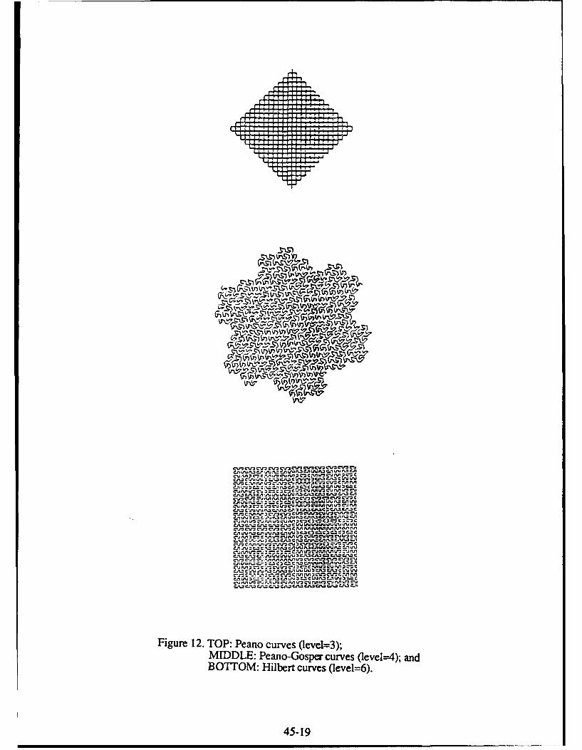
?. ;
Figure 12. Top: Peano curves (level=3);MIDDLE: Peano-Gosler curves (level---4); and
BOTFOM: Hilbert curves (level-6).
45-19

Al
X=T2 5ns I V- A2
Y=T'i'-"•''i'=•,._'• •i5ns I VY=TI l7- ~~A
-w
I ! ' ! 1 ! ' ' ! '
Figure 13. The output of the fractal program as captured on a digitizing oscilloscope.
45-20

AN ANALYSIS OF THE HIGHANGLE OF ATTACK AERODYNAMICS OF
ARBITRARY BODIES UNDER-GOINGRAPID MANEUVERS
Glenn GebertAssistant Professor
Department of Mechanical and Aerospace Engineering
Utah State UniversityLogan, UT 84322
Final Report for:Summer Faculty Research Program
Flight Vehicles Branch/Weapons Flight Mechanics DivisionArmament Directorate
Eglin AFB, Florida
Sponsored by:Air Force Office of Scientific Research
Bolling Air Force Base, Washington, D.C.
and
Utah State University
September 1993
46-1

AN ANALYSIS OF THE HIGH ANGLE OF ATTACKAERODYNAMICS OF ARBITRARY BODIES UNDER-GOING
RAPID MANEUVERS
Glenn A. GebertAssistant Professor
Department of Mechanical and Aerospace EngineeringUtah State University
Abstract
Little is known about the aerodynamics of finned missiles at high anglesof attack. There h-ve been several analytical approaches and only a fewexperimental studies. Virtually all high angle of attack research on slenderbodies has been concerned with the static aerodynamics. At large angles ofattack, a vortex dominated wake forms on the leeward side of the body.During rapid maneuvers (rapid pitching, yawing or rolling), the body andits fins translate through the vortical flow. As a result large, unsteadyforces and moments develop. The focus of this study was to develop aquick method for estimating the aerodynamics of rapidly maneuveringbodies. A discrete vortex approach was utilized for its ability to rapidlyestimate the gross high angle of attack aerodynamic loadings on finned andunfinned bodies. Significant modification of the aerodynamic loading isobserved, and the stability derivatives show large fluctuations for theunsteady motion. The discrete vortex method rapidly determines the flowcharacteristics of the body, and calculates the total body aerodynamics.
46-2

AN ANALYSIS OF THE TOTAL HIGH ANGLE OF ATTACKAERODYNAMICS OF ARBITRARY BODIES UNDER-GOING
RAPID MANEUVERS
Glenn A. Gebert
IntroductionThe development of supermaneuverable fighters has renewed an interest
in high angle of attack aerodynamics. Current fighter designs allow themto perform controlled maneuvers at angles of attack up to 70*. Although aconsiderable amount of work is being performed on the characteristics ofthe aircraft, little is known about the behavior of the weapons whenlaunched in such extreme flight conditions. Typically, a launching aircraftwill perform a high angle of attack maneuver (supermaneuver) only as alast resort. The maneuver is generally achieved wbnn the airplane has lostmost of its velocity, and tries one last time tc cessfully launch itweapons. Thus, it was the concern of this study to examine theaerodynamic characteristic of weapons at high incident angles and lowMach numbers.
Typically, the behavior of a weapons system is initially evaluated bydeveloping and running six degree-of-freedom (6-DOF) computersimulations. For these simulations, the aerodynamics of the body must beinput. It is known that at high angles of attack, the aerodynamics becomehighly non-linear. Thus, an aerodynamic database must be used in thesimulation rather than the usual low angle of attack linearized aerodynamicequations. This means that the aerodynamics for a large number of flightconditions must be determined.
An additional complication arises due to the fact that at moderate andhigh angles of attack, large out-of-plane loading (side force, yawing androlling moment) occur. Figure 1 shows a schematic of a finned body at ahigh angle of attack. A vortex dominated wake develops on the leewardside of the body. At moderate angles of attack, the vortices are largelysymmetric. At high angles of attack the vortex structure is still steady butasymmetric. At incidence, an axisymmetric body will develop in-planeloading (normal and axial force, pitching moment). However, due to thevortical wake, the in-plane loading will be modified and large out-of-plane
46-3

loading will occur. The out-of-plane loading is extremelydifficult to predict since theflow asymmetry is due toslight manufacturingimperfections at the nose tipof the body or disturbancesin the upstream flow.Although the vortices arelargely stable in time,conditions can change whichcause them to set updifferently into a new stableconfiguration and yield new Figure 1. Schematic of an Axisymmetric,
Slender, Finned Body at a Highloadings for the same flight Angle of Attackconditions.
The aerodynamic databases for use in 6-DOF simulations can essentiallybe generated in one of the four following ways, 1) Empirical Relations, 2)Wind Tunnel Tests, 3) Navier-Stokes Solutions, or 4) Discrete VortexMethods. Since few experiments have been done with high angle of attackbodies, no real empirical relations exist. Wind tunnel tests are too costlyfor design missiles, and Navier-Stokes solutions take too long to generateentire aerodynamic databases. The only present practical method for theproduction of entire high angle of attack aerodynamic databases arediscrete vortex methods. This lower order solution attempts to capture theessential physics of the flow while rapidly calculating the gross properties.
The usefulness of discrete vortex methods has been shown by a numberof researchers [Ref. 1-10]. Although the method does not give as detailedresults as other CFD solutions, it has the advantages of being very fast andstill determines the in-plane as well as the out-of-plane loadings. Thepresent study has extended previous discrete vortex analysis to include theeffect of unsteady motion of the body. In this analyses, the body canexperience pitching, yawing or rolling motion at given angles of attack andMach number. The stability derivatives are then calculated for theresulting data.
46-4

Theoretical DevelopmentA discrete vortex approach marches the flow solution down from nose
tip to the tail of the body. The downstream effects are neglible on theupstream flow. In subsonic flow, this is of course an approximation, but itleads to rapid solutions while still holding on to the dominate physics. Theflow at each cross flow section is analyzed as a two-dimensional flow. Ateach section, the boundary layer separates and a small amount of vorticityis injected into the flow. The upstream flows are convected to downstreamsections. The vortices of upstream sections are allowed to interact witheach other and the body, and they tend to roll up in large vorticalstructure. At an arbitrary axial location on the body, the cross flowvelocities are given in Ref. 8 as
w - iv = V.. sin(a)o (1)
where a- •• da
(a~~~~22 ________ __
•=2n - +- .1' +a2 +dx tan(a)• 2
2 i .. m. ( -C s,..,d.e"
"e C- a 2 - - ) 2xi-
where a is the angle of attack made by the body centerline and theupstream velocity vector. These equations give the velocity in complexvariables. Referring to the coordinate system shown in Fig. 1, the u, v,and w velocities are in the x, y, and z directions, respectively. Theposition of the point where the velocity is being calculated is specified as "= z + iy, where i = -T, and the x value gives the cross section location.The upstream velocity is V., a is the radius of the axisymmetric body atthe section, A, is a semi-infinite vortex weighting factor [Ref. 8], N is thenumber of shed nascent vortices at the sections, F is the strength of thevortices, and 4 is the complex location of each vortex. The overbar (-)denotes a complex conjugate. The equation is developed for the possibilityof Nf fins at the section which are modeled as source/sink sheets. Thestrength of each given panel along the fin is g, and the radial fins make an
46-5

angle 0 with the z axis. The source panels start at the location 'k and havea length Sk.,. The strengths of the source/sinks are found by standardcollocation techniques. The final term is due to the spinning of the body,and it will be discussed later.
The strengths of the shed vortices are found by integrating the vorticityacross the boundary layer at the point where is separates. As a result thevortex strength is
r -tan(a)2Ax (3)
where the value of 6)e is given by Eq. (2) evaluated at the separation pointin the previous step. Note that the calculation of the velocity field has beenwritten at discrete axial positions. Rather than continuous shedding ofvorticity, discrete vortices (nascent vortices) are introduced into the flow atgiven intervals. The separation locations are found using an integralboundary layer solver for both laminar and turbulent boundary layers.
For a known axisymmetric shape, angle of attack and flow velocity,Eqs. (1-3) define the potential incompressible flow field around a slenderfinned body. The upstream flows are assumed to convect to downstreamlocations at the axial velocity. Essentially the spatially developing flow istransformed into a time developing flow around a body of changing crosssection. The transformation is simply
x = V.cos(a)t (4)
The forces on the fins are found through sectioning the fins into panels,determining the actual angle of attack seen by each panel, and thendetermining the force on the panel by the following formula,
C,, = [Ao), sin(2a,) ±2.2 sin2(a,)]91 (5)
where CNf is the panel incompressible normal force coefficient, A. is thearea of the panel, w is a separation weighting factor which is set such thatS= r when as is less than the separation angle of 120, and o = 2.5 when
46-6

a, is greater than 12'. For the thin plate airfoils modeled, it was assumedthat the flow separates on the suction surface when the angle of attack isgreater than 120. The angle ap is the local angle of attack experienced bythe panel center, and Sref is the body reference area. This formula givesadequate behavior of the lifting surface aerodynamics. Since the equationis applied to each panel of the fin, the non-uniform upstream flow is takeninto account. The appropriate forces and moments are determined by theweighted sums of the equation over the panel.
All of the previous equations were developed for a uniform upstreamvelocity, a constant angle of attack, and roll angle. If the body isundergoing rapid maneuvers, the roll angle and angle of attack seen at eachsection will vary. Figure 2 shows schematically the velocity seen at eachsection. The cross flow velocity is due to the cross flow component of theupstream velocity and the component due to the pitching motion of thebody.
From Fig. 2 it is readily seen that the angle of attack seen as each axiallocation x along the body is
a =tan .sin(a)+(x- x)qV_ cos(a)
x
ws
Figure 2. Schematic of the velocity distribution of a pitchingbody at an angle of attack.
where as is the angle of attack seen at the given section, xcg is the axiallocation of the body center of gravity, and q is the pitching rate of thebody. Each section sees an apparent upstream velocity V'W of
46-7
v: jV sin(a)+(x-xo5 )q] +÷(V..cosa)" (7)
Since the equations are written in terms of a total angle of attack, the samerelations hold for a body with a yawing rate r as for a pitching body.
For a body experiencing roll, the final term of Eq. (2) must beintroduced to account for the roll. A single vortex is located at the centerof the body which induces a velocity equal to the roll rate at the bodysurface. Thus, in Eq. (2), the strength of the vortex F8 is
rF =2ra 2p (8)
where p is the roll rate. This term in the classic way accounts for theviscosity at the surface of the spinning body. This term must be includedwith the rest of the velocity field when utilizing the integral boundary layer
solver to determine the separation locations on the body. These integralmethods require that the flow is marched for the stagnation point to theseparation location.
For the rolling body, the definition of the stagnation point becomesmore difficult. In this analysis, the boundary layer solvers were marchedforward from the point where the potential flow velocity at the bodysurface is equal to (in magnitude and direction) the body rotation. For theboundary layer solution, the rotation rate is subtracted from the potentialflow for the driving potential flow (pressure gradient) in the boundarylayer equations. Thus, in this manner at the "stagnation" point, theimposed potential velocity in the boundary layer solver is identically zero.Away from the stagnation point, the potential velocity is adjusted
accordingly. This approximation of the boundary layer solver leads torapid solutions, and is in accordance with the approximate nature of thisapproach.
The fins on the nose tip are modeled as source/sink sheets as wasdiscussed. However, the fins are rolling with the body. Therefore, as theflow is marched from section to section, the fins move to different angularpositions at the appropriate rate. For an analysis with fins on the missile anestimation of the boundary layer separation point is made. If a fin iswithin the region of the body between the stagnation location and the
46-8

projected separation location, the flow is assumed to separate at the fin tip.If no fin is there, the flow integral boundary layer solver is run todetermine the separation location.
For the determination of the source/sink distribution on the fin and thestrength of the vorticity shed at the fin tip, the rotation of the fin must betaken into account. The velocity that the fin sees at any radial location dueto the rotation of the fin is vo = rip where ve is the velocity in the angulardirection, and rf is the radial location to a point on the fin. This additionalvelocity component must be included with the rest of the velocity fieldwhen determining the strength of the sources and sinks that will make thenormal component of the velocity at the fin surface equal to zero.
These changes were incorporated into a discrete vortex code namedDEVO, which stands for Discrete Elemental VOrtex program. The DEVOcode can handle a wide variety of slender body shapes, at total angles ofattack from 0' to 700, and Mach numbers from 0 to 5. For this analysis,only the low subsonic portions of the code were used. The modified codewas run on the Eglin AFB Cray YMP. Each solution took approximately15 minutes of CPU time, with the higher angles of attack requiring moretime as discussed in Ref. 8.
ResultsThe missile tested for this study is shown in Fig. 3. The body is an Air
Force AMRAAM without the wire harness. A full scale body was run sothe body diameter is 7 inches. All tests were run at a Mach number of0.15.
7.D .j 17.7 D If'-7.5DI
2.7 D - .74D- HI.77 D-.
Figure 3. Specifications of the AMRAAM-like missile used fortesting.
46-9

Figure 4 shows a computer image of the missile at 40' angle of attack.The image was generated using the YAPP program [Ref. I 1] developed atEglin AFB. In this figure, the body is not pitching. The figure shows thetotal pressure field calculated by the DEVO program at a particular crosssectional plane near the tail of the body. Additionally, the vortexformation on one side of the forward part of the body is shown. Althoughmore difficult to see without color, the total pressure shows the position ofthe vortices that exist near the body. As the body experiences pitchingmotion, the tail fins will convect through these vortices, and radically alterthe aerodynamics forces.
Figure 5 shows a similar computer image of a missile pitching at q =
2.0 rad/s, and at a 400 angle of attack. By comparing with Fig. 4, it can beseen that the flow field significantly changes from the static aerodynamiccase. The changes in the flow field cause significant changes in the bodyaerodynamics.
Figure 4. Computer generated image of a missile and flow fieldfor a static flight attitude of Mach = 0. 15 and 40' angleof attack.
46-10

Figure 5. Computer generated image of the surrounding flowfield and the missile pitching at q =2.0 radls at a Mach= 0. 15 and 400 angle of attack.
Derivative of Normal Force wrt Pitching Ratech=0.15, "X", - Configuration
a, Alpba .
-~ - -Alpha -I51 0 -
SAipha - 25 80/
60U
-47 -. 5 -2. 5 - 2 -1.5 -1 -0 ..5 -2001
Pitch Rate (q)
Figure 6. Stability derivative of the normal force wrt the pitching
rate for various low and moderate angles of attack.
46-11

Derivative of Normal Force wrt Pitching RateMach - 0.15, "X" - Configuration
•°°°oool3
A400
.6000
C 2 0-4 -3 -. -1w 5 0 1Pitch Rate (q)
Figure 7. Stability derivative of the normal force wrt the pitchingrate for various high angles of attack.
Figures 6 through 15 show the stability derivatives for a pitching missile.The body is flying in an "x"-configuration. Figures 6 and 7 show thederivative of the normal force with respect to the pitch rate. The stabilityderivative is defined in the usual way as C.. = aCz/a(qL22V1). The
Derivative of Pitching Moment wrt Pitching RateMach - 0.15, "X" - Configuration
-4 -3.5 •-3 -2.5 | -2 -1.5 -1 -0.51000 ,
O00
-a3
.54000
-6000
Alpha = 1• -7000
Alpha = 25 Pitch Rate (q)
Figure 8. Stability derivative of the pitching moment wrt the pitchingrate for various low and moderate angles of attack.
46-12

Derivative of Pitching Moment wrt Pitching RateMach = 0.15, "X" - Configuration
40000-
330000-
Pitch002ate0(q)
Howve, iti paetfomtefgrsta atteloe 2nge0f(tak
- 00-50000 •
th s.tbl d vt5 i -r0000
lAlg al e 55 Pitch Rate (q)
Figure 9. Stability derivative of the pitching moment wrt thepitching rate for various high angles of attack.
prediction of this derivative is rather difficult both analytically andexperimentally. The figures show considerable scatter of the data.However, it is apparent from the lower angles of attack,the stability derivative is reasonably well behaved, and at moderate andlarge angles of incidence, considerable scatter occurs in the data.
Figures 8 and 9 show the pitch damping derivative with respect to thepitch rate. As with the normal force, the curves are best behaved at lowangles of attack. As the angle of attack increases, the derivatives becomemore irregular. This behavior is due to the motions of the lifting surfaces
through the wake vorticity. The overall angle of attack seen by a surface
can rapidly change from positive to negative, as it moves through the
vortex core.
The out-of-plane stability derivatives for pitching motion are shown inFigs. 10-15. It is expected that the out-of-plane loading will be even more
erratic than the in-plane since the entire loading is due to the asymmetric
vortex formation. The figures do show highly non-linear behavior at
moderate and high angles of attack. However, at low angles of attack as
seen in figures 10, 12, 14, the out-of-plane stability derivatives are all quite
small. This is probably due to the fact that the out-of-plane loading itself isquite small at low angles of incidence.
46-13
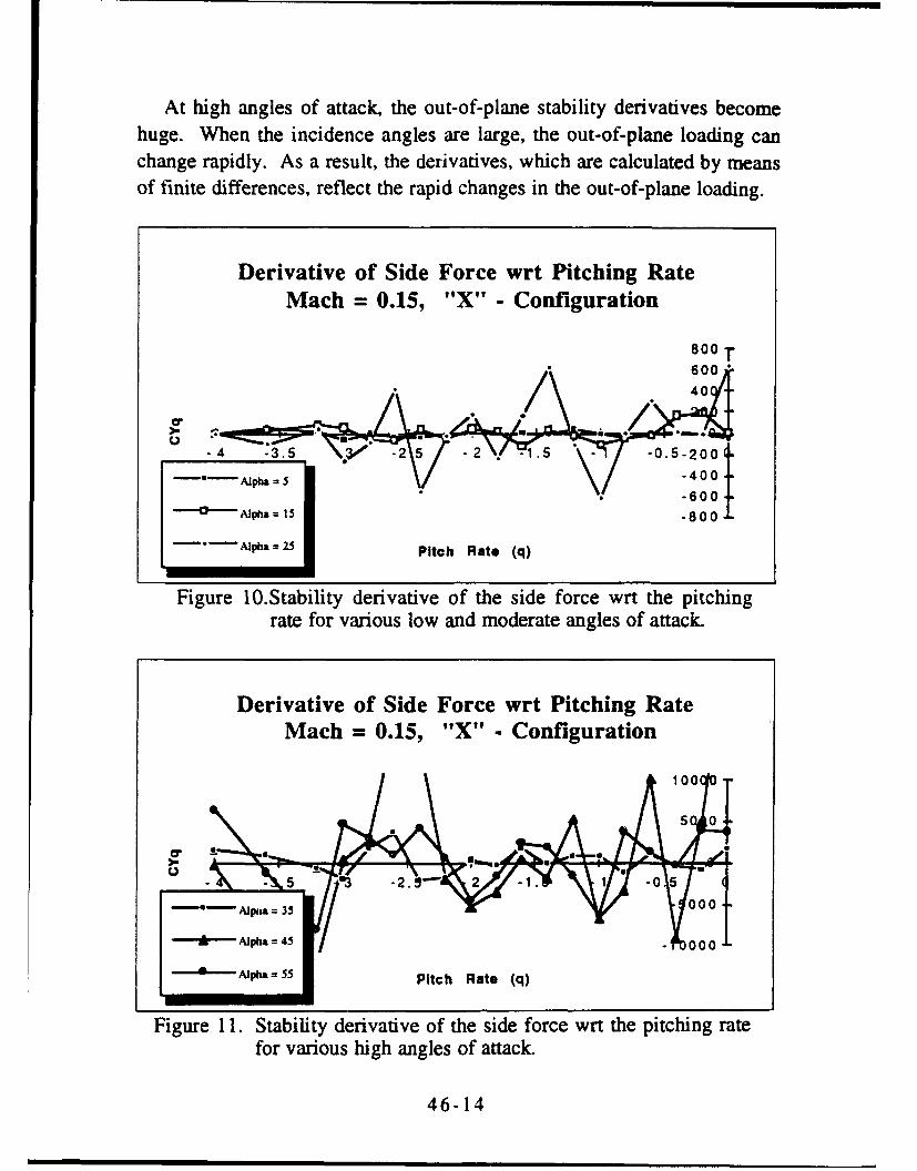
At high angles of attack, the out-of-plane stability derivatives becomehuge. When the incidence angles are large, the out-of-plane loading canchange rapidly. As a result, the derivatives, which are calculated by meansof finite differences, reflect the rapid changes in the out-of-plane loading.
Derivative of Side Force wrt Pitching RateMach = 0.15, "X" - Configuration
*800T
600 "
-400-
• -6. 00 -
• Alpha = 15 -800.--
-Alpha = 25 Pitch Rate (q)
Figure 1O.Stability derivative of the side force wrt the pitchingrate for various low and moderate angles of attack.
Derivative of Side Force wrt Pitching RateMach = 0.15, "X" - Configuration
-- ' Alipa = :35
J, Aipha = 45
II- Alha=55Pitch Rate (q)
Figure 11. Stability derivative of the side force wrt the pitching rate
for various high angles of attack.
46-14

Derivative of Yawing Moment wrt Pitching RateMach = 0.15, "X" - Configuration
4000
30020
Crz
A -3- 0.51000•-- '-..Upb .5 -2000-
Alpa = -3000 -£ •J•= 15-4000-
- Alpha = 25 Pitch Rate (q)
Figure 12. Stability derivative of the yawing moment wrt the pitchingrate for various low and moderate angles of attack.
Derivative of Yawing Moment wrt Pitching RateMach= 0.15, "X" - Configuration
' Alpha = 35 250000
SAlpha = 45 200000
-JOO"•- .•pb = 55.1000q•-Alph -3 5 5 3 2. - . O, 0 j)
-100000
Pitch Rate (q)
Figure 13. Stability derivative of the yawing moment wrt thepitching rate for various high angles of attack.
46-15
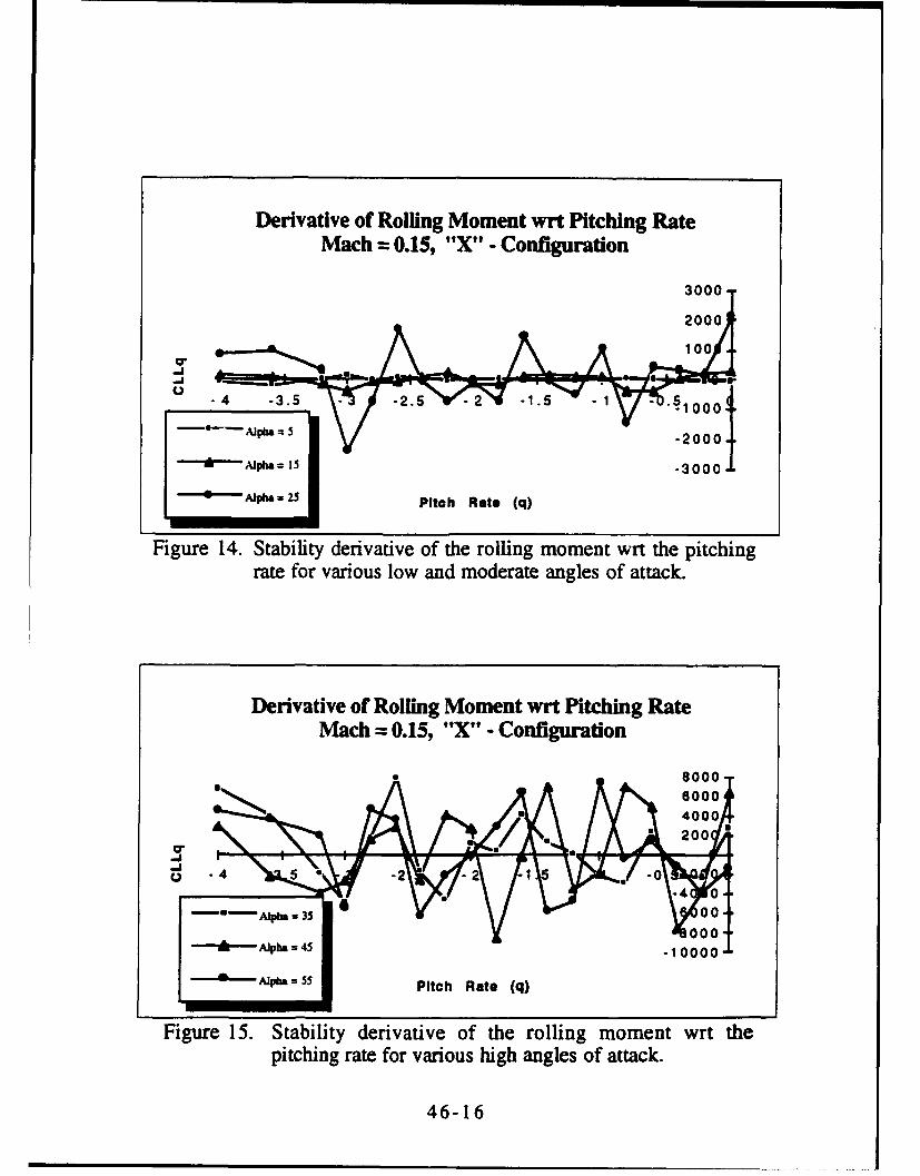
Derivative of Rolling Moment wrt Pitching RateMach -0.15, "X" - Configuration
3000-
20003100
-o -4 -3.5 -2.5 2 -1.5 1.. 0001"
• --- Alpha = 5 -2000-
.t Alphat = 15 -3000-
Al•pha - 25 Pitch Rate (q)
Figure 14. Stability derivative of the rolling moment wrt the pitchingrate for various low and moderate angles of attack.
Derivative of Rolling Moment wrt Pitching RateMach = 0.15, "X" - Configuration
-10000m• 2000I10,
,, - 4-2. 10
4 0- 0 Alpha = 35 -1 000
"-Apha = 55 Pitch Rate (q)
Figure 15. Stability derivative of the rolling moment wrt thepitching rate for various high angles of attack.
46-16

The side loading can rapidly change sign and magnitude for a very smallchange in pitching rate which results in the large derivatives.
For the out-of-plane loading, the curves should not be used to determinethe actual value of the stability derivatives, but give an indication of thedependence of the out-of-plane loading on the motions of the body. Thefigures give a good indication that the out-of-plane loading is of negligibleimportance at low angles of attack. However, at high angles of attack,there is considerable effect not only in the static loading, but also thestability derivatives.
Figures 16-19 show the derivatives of the aerodynamic coefficients withrespect to roll rate. As with the pitching body, the body experiencing rollhas reasonably well behaved stability derivatives at low angles of attack,but extremely large and fluctuating derivatives at the high incidence angles.For brevity, only the out-of-plane loadings are given here.
The derivative of the side force with respect to roll rate is shown inFig. 16. Only the high angle of attack results are shown here. The forceshows considerable effect of roll rate roll coupling, and the results aresimilar for the normal force. The graph shows that the higher the angle ofattack, the larger the overall magnitude of the stability derivative.
Derivative of Side Force wrt Rolling Rate Mach = 0.15,"X" - Configuration
3000,
2000-
100 1 -5 -- Alpha = 35o2000
-""•'Alpha a 45-3000 -.
Roll Rate (p)
Figure 16. Stability derivative of the side force wrt the rolling ratefor various high angles of attack.
46-17
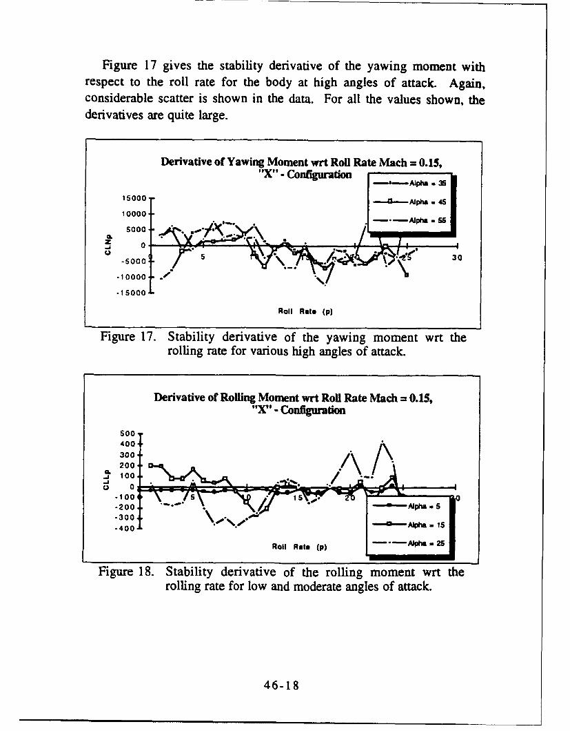
Figure 17 gives the stability derivative of the yawing moment withrespect to the roll rate for the body at high angles of attack. Again,considerable scatter is shown in the data. For all the values shown, thederivatives are quite large.
Derivative of Yawing Moment wrt Roil Rate Mach = 0.15,"X- Configuration
"----.-Alpha - 35
15000 -- & Alpha 4610000 j-- Apha .55
5000z 0
.0
O 5 30-5000
-15000-
Roll Rate (p)
Figure 17. Stability derivative of the yawing moment wrt therolling rate for various high angles of attack.
Derivative of Roiling Moment wrt Roll Rate Mach = 0.15,-xC -Configuration
500-400
300-200-a
..j 100-
o 0-100 A I is 0- 2 0 0 -." ' " .•"-- 4 ' A lp h a .a 5
- 3 0 0 - -•, - A lP h a a 15' -Alpha
.. 25Roll Rate (p) il
Figure 18. Stability derivative of the rolling moment wrt therolling rate for low and moderate angles of attack.
46-18

Derivative of Rolling Moment wrt Roll Rate Mach = 0.15,"xie- Confguration
3000
2000
1000.
0.
0 -10001 .Apa-3-2000-
-3000
-4000
Roll Rate (p)
Figure 19. Stability derivative of the rolling moment wrt therolling rate for high angles of attack.
The last two figures show the derivative of the rolling moment with respectto the rolling rate. Figure 18 shows the stability derivative at low andmoderate angles of attack, and Fig. 19 gives it at high angles of attack.Note that at low angles of attack, the roll damping derivative is rathersmall and nearly constant. However, as the angle of attack is increased, thederivative gets increasingly large, and oscillates with the roll rate. Thiseffect is due to the fins rolling through the core of the shed vorticity, andinducing large forces and moments on the fins in doing so.
In the past, little time has been spent in the study of finned slender
bodies at high angles of attack. It is known that for certain geometries in arange of high angles of attack, large symmetric or asymmetric vorticalstructures form on the leeward side of the body. When lifting surfaces areon the body, the interaction between the vortical flow and the fins cansignificantly affect the overall forces and moments of the body. Previousresearch has employed various techniques to estimate the staticaerodynamic loading on the body, but apparently no studies have ever beenconducted on the aerodynamics of maneuvering finned bodies.
The present study attempted to estimate the stability derivatives of abody undergoing rapid pitching, yawing, and rolling. A discrete vortex
46-19

method was used to rapidly determine the total aerodynamic loading. Anexisting discrete vortex code was modified to account for the effects of amaneuvering body. The result showed significant interaction between thelifting surfaces and the vortical structures of the flow.
The estimated stability derivatives were shown to behave reasonablywell and remain more or less constant at low angles of incidence.However, at moderate and high angles of attack, the stability derivativesshowed extremely non-linear behavior. The motion of the lifting surfacesthrough the vortical flow quickly changes the loading on the body leadingto extremely large stability derivatives.
This study has shown that a possibility for gross error in the estimationof the total high angle of attack body aerodynamics can exist if the effectsof pitching, yawing, and rolling are neglected. Further research needs tobe performed (both analytical and experimental) in this area. This initialwork has pointed to a possible problem, but more detailed studies need tooccur.
References
1. Wardlaw, A. B., "Prediction of Normal Force, Pitching Moment, andYawing Force on Bodies of Revolution at Angles of Attack up to 50Degrees Using a Concentrated Vortex Flow-Field Model," NOL TR 73-209, Oct. 1973.
2. Wardlaw, A. B., "High Angle of Attack Missile Aerodynamics,"AGARD LS-98, Feb. 1979, pp. 5.1-5.53.
3. Marshall, F. J. and Deffenbaugh, F. D., "Separated Flow Over Bodiesof Revolution Using Discrete Vorticity Cross Wake," NASA CR-2414,June 1974.
4. Thomsom, K. D. and Morrison, D. F., "The Spacing, Position, andStrength of Vortices in the Wake of Slender, Cylindrical Bodies at LargeIncidence," Journal of Fluid Mechanics, Vol. 50, 1971, pp. 751-783.
5. Angelucci, S. B., "A Multivortex Method for Axisymmetric Bodies atAngle of Attack," Journal of Aircraft, Vol. 8, Dec. 1971, pp. 959-966.
46-20

6. Mendnehall, M. R. and Lesieutre, D. J., "Prediction of VortexShedding from Circular and Noncircular Bodies in Subsonic Flow," NASACR 4037, Jan 1987.
7. Mendnehall, M. R. and Perkins, S. C., Jr., "Vortex Cloud Model forBody Vortex Shedding and Tracking," Tactical Missile Aerodynamics,edited by M. J. Hemsch and J. N. Nielson, Vol. 104, Progress inAstronautics and Aeronautics, AIAA, N.Y., 1986, pp. 519-571.
8. Gebert, G. A. "Determination of Slender Body Aerodynamics UsingDiscrete Vortex Methods," accepted for publication in the AIAA Journal ofSpacecraft and Rockets, November 1992.
9. Mendnehall, M. R. and Lesieutre, D. J., "Prediction of SubsonicVortex Shedding from Forebodies with Chines," Journal of Aircraft, Vol.29, No. 3, May-June 1992, pp. 404-412.
10. Gebert, G. A. "Discrete Vortex Methods for the Determination ofFinned Body Aerodynamics," submitted to the AIAA Journal of Spacecraftand Rockets, April 1993.
11. Belk, D. and Maple, R., "Visualization of Vortical Flows with YetAnother Post Processor," AIAA Aerospace Sciences Meeting, Reno,NV, Paper 93-0222, Jan. 1993.
46-21
HOLOGRAPHY OF EXPLODING SHELLS
James S. Marsh
Professor
Department of Physics
The University of West Florida
Pensacola, FL 32514
Final Report for:
Summer Faculty Research Program
Wright Laboratory
Armament Directorate
WL/MNSI, Eglin AFB
Sponsored by:
Air Force Office of Scientific Research
Bolling Air Force Base, Washington, D.C.
August 1993
47-1

HOLOGRAPHY OF EXPLODING SHELLS
James S. MarshProfessor
Department of PhysicsThe University of West Florida
Abstract
A holography laboratory was set up and the capability to
produce high quality transmission and reflection holograms was
developed as the first phase of a project to make cylindrical
holograms of exploding shells.
47-2

HOLOGRAPHY OF EXPLODING SHELLS
James S. Marsh
Introduction
Holograms of rapidly moving objects were produced as early
as 1966 by Brooks et. al. (1966), on flat plates using a multi-
mode ruby laser. For objects moving with supersonic speeds, and
with the geometries available, a hologram of the actual object is
not obtained. Rather the object is viewed against a bright
background, and a kind cZ holographic shadowgram is produced.
The shadowgram is a three d-mensional object and perspective
changes are observed in the hologram as the viewing angle is
changed.
The Armament Directorate is interested in studying the
dynamics of shell fragments produced by exploding shells. A
pilot program to investigate the feasibility of making cylindri-
cal holograms of exploding shells, using pulsed laser light from
a multimode ruby laser, was assigned to LTV in 1989. The suc-
cessful outcome of that program showed (Hough and Gustafson,
1989) that high quality single and double pulsed holograms could
!ndeed be made. These holograms allow scanning of the shell
fragment field through a full 180 degree arc. This is important
in order to determine, in three dimensions, the positions and
shapes of the fragments. The dimensional stability problems
associated with film shrinkage, reconstruction with wavelengths
different from that of the
47-3

radiation used to make the hologram, etc., were solved by super
imposing a holographic image of a standardized cylindrical grid
on the hologram. By double pulsing the ruby laser at a suitable
time interval it was possible to produce a double exposure holo-
grair that allowed the vector velocity of each of the fragments to
be determined.
Methodology
With the success of the pilot program, it was decided to set
up a facility at Eglin AFB for the purpose of routine holographic
imagery of exploding shell fragments. A ruby laser capable of
producing a 3 joule pulse in a 20 nanosecond time frame, in
either single or double pulse mode, was purchased. This instru-
ment, in addition to a 60 milliwatt Helium-Neon Laser, darkroom
hardware and chemicals, and assorted optical hardware, was on the
scene when I arrived in May to assist with the optical issues
involved in setting up the facility and bringing it to a state in
which high quality holograms could be produced as necessary in a
routine manner. The facility adjoins a long tunnel in which the
gun will be fired. The tunnel is connected to the facility by
means of a 6 inch port drilled into the wall separating the two.
The work this summer resulted in the routine production
within the facility of high quality single beam and double beam
transmission and reflection holograms using the 60 milliwatt He-
Ne laser. These are
47-4
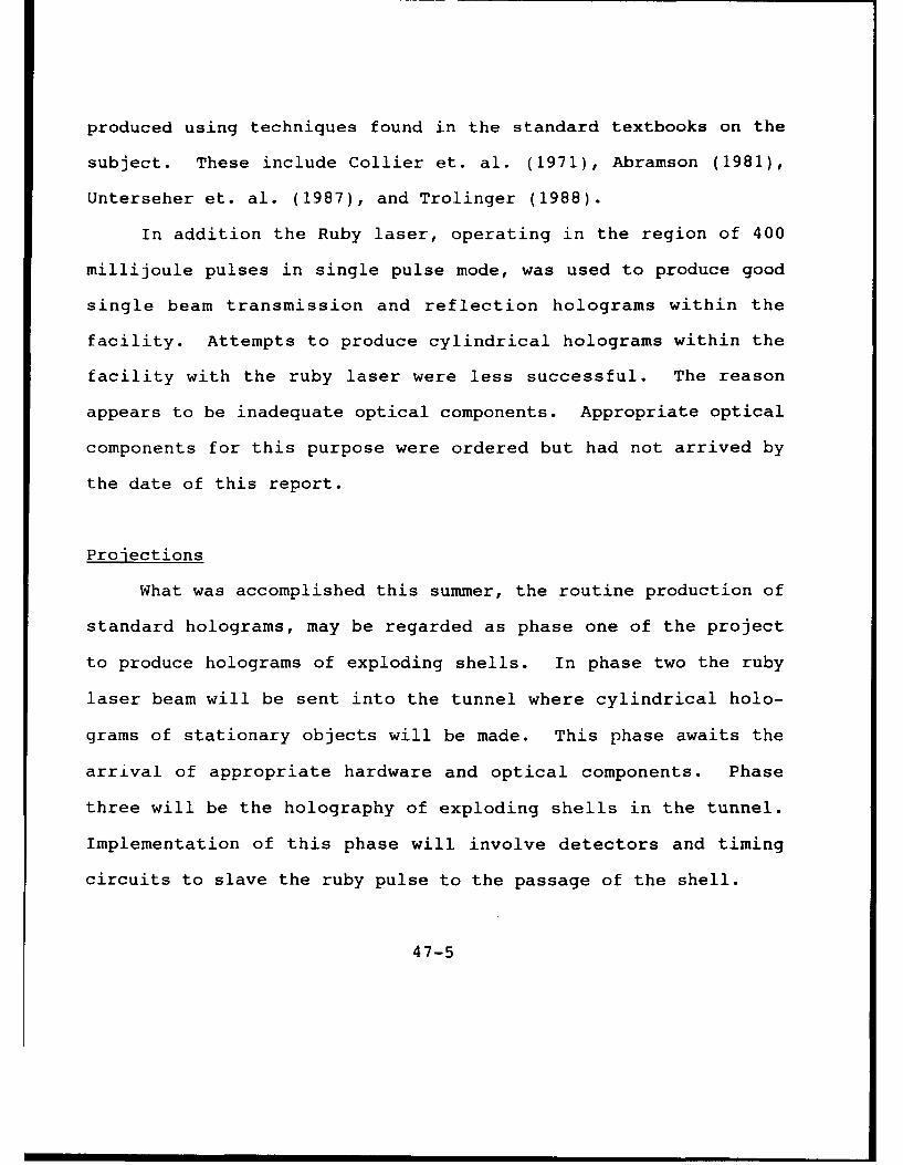
produced using techniques found in the standard textbooks on the
subject. These include Collier et. al. (1971), Abramson (1981),
Unterseher et. al. (1987), and Trolinger (1988).
In addition the Ruby laser, operating in the region of 400
millijoule pulses in single pulse mode, was used to produce good
single beam transmission and reflection holograms within the
facility. Attempts to produce cylindrical holograms within the
facility with the ruby laser were less successful. The reason
appears to be inadequate optical components. Appropriate optical
components for this purpose were ordered but had not arrived by
the date of this report.
Projections
What was accomplished this summer, the routine production of
standard holograms, may be regarded as phase one of the project
to produce holograms of exploding shells. In phase two the ruby
laser beam will be sent into the tunnel where cylindrical holo-
grams of stationary objects will be made. This phase awaits the
arrival of appropriate hardware and optical components. Phase
three will be the holography of exploding shells in the tunnel.
Implementation of this phase will involve detectors and timing
circuits to slave the ruby pulse to the passage of the shell.
47-5
BIBLIOGRAPHY
N. Abramson, "The Making and Evaluation of Holograms," Academic
Press, New York, (1981)
R. E. Brooks, L. 0. Heflinger, and R. F. Wuerker, "Pulsed Laser
Holograms," IEEE J. Quantum Electron. QE-2, 275 (1966)
R. J. Collier, C. B. Burkhardt, and L. H. Lin, "Optical Hologra-
phy," Academic Press, New York (1971)
G. R. Hough and D. M. Gustafson, "Ballistic Applications of
Lasers," SPIE Volume 1155, Ultrahigh Speed and High Speed Photog-
raphy, Photonics, and Videography '89, pp. 181-188, (1989)
J. D. Trolinger, "Laser Applications in Flow Diagnostics," AGAR-
Dograph No. 296, (1988)
F. Unterseher, J. Hansen, and B. Schlesinger, "Holography Hand-
book," Ross Books, Berkeley, CA (1987)
47-6
A Methodology for Missile Autopilot Performance Enhancementin the Presence of Multiple Hard Nonlinearities
Armando A. RodriguezAssistant Professor
Deptartment of Electrical Engineering
Arizona State UniversityCenter for System Science & Engineering
Tyler & Rural, GWC 612Tempe, AZ 85287-7606
Final Report for:Summer Research Program
Wright Laboratory
Sponsored by:Air Force Office of Scientiffic ResearchWL/MNAG, Eglin Air Force Base, FL.
September 30, 1993
48-1
A Methodology for Missile Autopilot Performance Enhancementin the Presence of Multiple Hard Nonlinearities
Armando A. RodriguezAssistant Professor
Deptartment of Electrical EngineeringArizona State University
1 Abstract
The primary goal of this research effort has been to develop systematic design methods for enhancingthe performance of missile autopilots. To focus the research, efforts have concentrated on the importantproblem of guaranteeing performance in the presence of multiple hard nonlinearities. Hard nonlinearitiesinclude, for example, saturating actuators, rate limiters, etc. Traditionally, engineers have accommodatedsuch nonlinearities by "extending" single-input single-output (SISO) ideas, using "engineering judgement",and conducting extensive simulation. Because the SISO ideas do not extend well to multiple-input multiple-output (MIMO) problems, the techniques used have not been systematic and, more than often, have resultedin overly conservative designs. The methods developed in this research systematize the design process with-out sacrificing performance. More specifically, the methods are applied to an EMRAAT BTT missile withsaturating actuators. It is shown that the introduced performance enhancement system significantly im-proves autopilot performance by maintaining desired directionality properties, eliminating wind-up effects,and above all guaranteeing stability.
Contents
I Abstract 48-2
2 Motivation 48-3
3 Overview of Research 48-3
4 Performance Enhancement Methodology 48-44.1 Nominal Model for EMRAAT BTT Missile ...... ............................ 48-44.2 Nominal Autopilot Design .............................................. 48-44.3 Method for Accomodating Saturating Actuators .............................. 48-84.4 Computational Issues ........ ........................................ 48-114.5 Application of Method to EMRAAT BTT Missile .............................. 48-124.6 Unstable Operating Points and Other Hard Nonlinearities ........................ 48-124.7 More General Nominal Compensation Schemes ................................ 48-15
5 Significance of Work 48-15
6 Additional Collaborative Work 48-156.1 Computation of Structured Singular Value Using Genetic Algorithms ................ 48-156.2 Performance Enhancement for Guidance Systems . ............................ 48-166.3 Extension to Gain-Scheduled Controllers .................................... 48-16
7 Summary & Directions for Future Research 48-16
8 Bibliography 48-16
9 Appendix: Proposal for Invited Session to 1994 ACC 48-18
48-2
A Methodology for Missile Autopilot Performance Enhancementin the Presence of Multiple Hard Nonlinearities
Armando A. Rodriguez
2 Motivation
This research is motivated by the lack of systematic procedures for designing full envelop autopilots formissiles. This defficiency is particularly crucial in the design of autopilots for high performance missilesystems. For such systems, hard nonlinearities such as saturating actuators and rate limiters become acritical concern because they degrade system performance. Such nonlinearities may alter the directionalityproperties of the autopilot, cause dynamic wind-up, and induce instability. These effects may significantlyaffect the miss distance and are of particular concern during the terminal phase of an air-to-air engagementwhen evasive target maneuvering may require abrupt control actions. In this section, a method for enhancingthe performance of such systems is presented. The focus is on maintaining performance in the presence ofsaturating actuators. Other types of nonlinearities are also discussed.
Traditionally, control design for missile systems has been based on gain-scheduling [8]. Gain-schedulingis a method whereby linear controllers, based on linear models of the true nonlinear system, are "pieced"together over the operating envelope of the system. The initial designs often do not take into account theeffects of hard nonlinearities. One motive for this research has been the lack of systematic methods to modifythe original designs so that such nonlinearities can be accommodated.
For physical reasons, system designers often want to limit certain variables (e.g. angle of attack, sideslipangle, roll rate, etc.). Typically, adhoc modifications are employed and extensive simulations must be per-formed to justify the modifications. A procedure for systematizing this process over the full envelope of thesystem has been another motive for this research.
3 Overview of Research
Typically, initial autopilot designs are based on linear models and neglect nonlinearities such as saturatingactuators [1], [2]. Traditionally, such nonlinearities have been addressed in a conservative manner; sacrificingperformance to satisfy some "small-gain" design criterion [10], [20]. For single-input single-ouput (SISO)systems, methods have been developed which improve performance. These method, however, do not extendwell to multivariable applications [7].
In this work, it is shown how the initial autopilot design can be modified to accommodate the saturatingactuators without sacrificing performance. The idea is to introduce a saturation detection system whichmaintains, to the extent possible, the multivariable properties of the original autopilot design [5], [6], [7]. Inthis paper, it is shown how to construct such a system for a generic EMRAAT (Extended Medium RangeAir-to-Air Technology) missile operating near the terminal phase of an air-to-air intercept [1].
An autopilot with prescribed directionality specifications is used. It is shown how saturating actuatorsresult in wind-up effects and destroy the intended directionality properties by preventing the autopilot fromproperly coordinating the fin commands. The original autopilot is then modified by introducing a perfor-mance enhancement system. The addition is shown to markedly improve the performance of the originalautopilot. Moreover, the modification scheme not only comes with nominal stability guarantees, but alsoeliminates wind-up effects and maintains, to the extent possible, the directionality properties of the originaldesign. Finally, insight is given into how the method presented can be extended to systematize the designof general nonlinear autopilots.
48-3

4 Performance Enhancement Methodology
In this section, a systematic control system design methodology is proposed for maintaining performance inthe presence of saturating actuators. Other hard nonlinearities are also addressed.
4.1 Nominal Model for EMRAAT BTT Missile
Throughout this research, the focus has been placed on enhancing performance for highly maneuverableBank-to-Turn (BTT) missile systems with multiple saturating actuators. BTT missiles offer higher maneu-verability over conventional Skid-to-Turn (STT) missiles by the use of an asymmetrical shape and/or theaddition of a wing [1], [2]. The model used for this study is for an EMRAAT BTT missile. For simplicity,focus has been placed on the yaw/roll dynamics with
Mach number = 2.5
Qpres = 1720 lb/ft2
a = 20 degrees.
The model is given by the following system of ordinary differential equations [1]:
ip = Apzp + Bpup (1)Y CPZP (2)
where
-.818 -0.999 0.349 = 0. 147 0.0121 C= 0AP = 80.29 -0.579 0.009 Bp -194.4 37.61 0 1 0 (3)
-2734 0.5621 -2.10 -2176 -1093
UP [rudder aileron IT (4)
ZP= [ sideslip yawrate rolirate IT (5)
y = [ sideslip yawrate IT (6)
and all variables are measured in degrees. This system has poles at s = -0.6579,-1.4195 ± j32.1542. Thesingular values of the above missile (plant) transfer function matrix P(s) = G,(sI - Ap)- 1 Bp are shown inFigure 1.
4.2 Nominal Autopilot Design
For purposes of demonstrating the performance enhancement concept, the LQG/LTR design methodology[21] was used to obtain a nominal linear autopilot design. The procedure is now described.
Stepi: Form Design Plant. To guarantee zero steady state error to step commands, the plant P wasaugmented with integrators; one in each control channel. The resulting system is called the design plant. Ithas a state space triple [Ades, Bde,, Cdes] given by
Ades [o o)0] B [,. [ Cd[[0 C, (7)Ad 1 Bp Ap 0
The design plant singular values have been plotted in Figure 2.
48-4

.00(a) Plant Singular Values: Yaw/Roll Dynamics
00 .. . . . .. .. . .. . . .. . . . .
- 50 ....
-10 .. . .... .. . . . .
-1501-10-1 10) 101 102 103 106
frequency (rad/sec)
Figure 1: Plant Singular Values
(b) Design Plant Singular Values
50 ... . ......
A~ -100.....
-200,10-1 10) 101 102 103 l04
frequency (rad/sec)
Figure 2: Design Plant Singular Values
48-5

Step2: Design Target Loop. The next step in the process is to design the target (desired) open looptransfer function matrix. The target loop was selected to have a state space triple [Ad.,, H, Cd,,] where thefilter gain matriz H was selected to be
-0.1036 -0.0055[-0.0003 0.0912 1 -4.8067 0.0009
10 [v(:,4) - v(:,5)] -1.6482 -1.7159 2.0003 0.0000 (8)~ -. 642 -. 719 J0.0003 2.0000
4.8980 5.7272
wherev 4 =[ 0.0009 0 -0.0001 -0.3296 -0.9441 ]Tandvs=[ 0 0.0440 -0.0182 0.3432 0.9381 ]Tare right eignenvectors of Ade corresponding to the eigenvalue A = 0. This makes the pair (Ad.., H) un-controllable because the left eigenvectors of Ad., associated with the missile modes lie in the left null spaceof H. By so doing, one obtains the target singular values shown in Figure 3. Here, H has been deliberatelyselected so that the target loop looks like an 'integrator" with gain crossover frequency near 2 rad/sec.
Step 3: Recover Target Loop. The next step in the process is to recover the target loop by solvingan appropriately formulated cheap control problem. This amounts to solving the Control Algebraic RiccatiEquation (CARE)
0 = KýAde. + A T ,Kc + TjsCe cBe 1 BT KK~d.+~+ C•,Cd.. - KC Bd.-Bd' K. (9)P
for the unique symmetric positve definite solution Kc. This was done with a recovery parameter p of
p = 10-6 (10)
Doing this yields the control gain matrix
"_ I B [ 612.4440 -88.1472 -410.4327 -965.3118 -1.7612 1P dBeK = -88.1472 164.2489 -564.4860 254.7471 -7.1359
The final compensator, K (cf. Figure 5), is then given by
= Ax + Be (12)
U = Cz (13)
where e = r - y and
A = Ades - BdesGa - HCdQ. (14)
B=H (15)
C = GP (16)
A balanced realization for K = [A, B, C] is then given by
-0.2903 -107.7837 6.6692 -2.5820 -0.4031107.6795 -97.8098 63.9509 -4.5172 -5.3516
A = -6.7247 64.8158 -54.1931 -40.7948 5.1149 (17)3.2148 2.0979 29.5571 -631.1537 429.88940.3648 -3.3887 3.0907 -460.0290 -0.7433
2.2840 0.4772-40.7546 2.1291
B = 18.4665 -0.2215 (18)-2.0715 -44.6786-0.9753 -1.1753
48-6

..... (c) Target Lo~op Singular Values
2 0
0 .. .. . . . . . . . ....
~-20
100)IO 101 102 103 104
frequency (rad/sec)
Figure 3: Target Loop Singular Values
50........(d) Recovered & Target Loop Singular Values
0 ... . ..
S-50 ............... :7
10 .. .. ... .... .. ... .. . .. . .
-150 ..
10-1 10) 101 102 103 104
frequency (rad/sec)
Figure 4: Recovered and Target Loop Singular Values
48-7

r e K y
Figure 5: Visualization of Nominal Closed Loop System
C= [0.8562 8.5376 -1.7085 43.9089 1.1235] (19)I2.1706 39.9071 -18.3886 -8-.5133 1.0346
The recovered singular values have been plotted in Figure 4.In what follows, the discrete-time realization
X =Az + Ben (20)
un = Czn (21)
where
A=I+ TA B=T.B C=C T, = O.Olsec (22)
will also be used for K.
4.3 Method for Accomodating Saturating Actuators
While a Research Associate at Eglin Air Force Base, the principal investigator focussed on the problem ofenhancing performance in the presence of multiple saturating actuators [16]-[19]. The methods developedare based on the work of [7] and the more recent work of [5].
Let P denote a linear time invariant (LTI), multiple-input multiple-output (MIMO) plant. Let K denotea LTI MIMO compensator with state space triple [A, B, C]. The following assumptions will be made on Pand K.
Assumption 4.1 (Assumptions on P and K)It will be assumed that
(1) P is stable.
(2) K has been designed so that the closed loop system in Figure 5 has desirable properties .
(3) K is neutrally stable'.
(4) The pair (A, C) is observable.
UThe case where P is unstable will be discussed subsequently. The compensator K may be designed using anylinear design methodology (e.g. 7i', Wt2 , £, LQG/LTR, etc.) [11]. If a complex missile model is available,the methods described in [121-f15] may prove useful.
le.g. robust performance, etc.2 The matrix A may have eigenvalues on the imaginary axis so long as each has an associated eigenvector; i.e. the geometric
and algebraic multiplicities coincide. Repeated roots with geometric defficiency are not permitted here. This assumption is notrestrictive for missile autopilots.
48-8
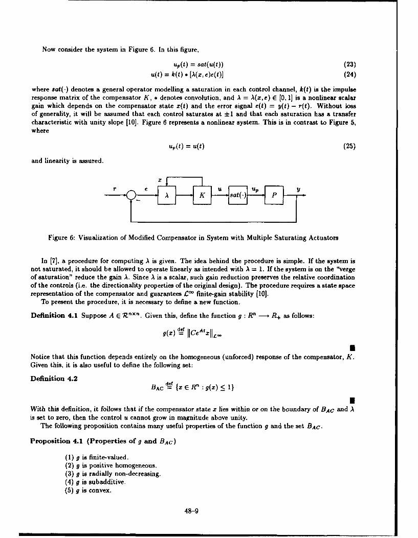
Now consider the system in Figure 6. In this figure,
up(t) = sat(u(t)) (23)
u(t) = k(t) * [A(z, e)e(t)] (24)
where sat(.) denotes a general operator modelling a saturation in each control channel, k(t) is the impulseresponse matrix of the compensator K, * denotes convolution, and A = A(z, e) E [0, 1] is a nonlinear scalargain which depends on the compensator state z(t) and the error signal e(t) = y(t) - r(t). Without lossof generality, it will be assumed that each control saturates at ±-1 and that each saturation has a transfercharacteristic with unity slope [10]. Figure 6 represents a nonlinear system. This is in contrast to Figure 5,where
uP(t) = u(t) (25)
and linearity is assured.
re A K U sat(.) U P Y
Figure 6: Visualization of Modified Compensator in System with Multiple Saturating Actuators
In [7], a procedure for computing A is given. The idea behind the procedure is simple. If the system isnot saturated, it should be allowed to operate linearly as intended with A = 1. If the system is on the "vergeof saturation" reduce the gain A. Since A is a scalar, such gain reduction preserves the relative coordinationof the controls (i.e. the directionality properties of the original design). The procedure requires a state spacerepresentation of the compensator and guarantees £C finite-gain stability [10].
To present the procedure, it is necessary to define a new function.
Definition 4.1 Suppose A E RV"'". Given this, define the function g : Rn -+ R+ as follows:
g J) ICeA1Xll _
Notice that this function depends entirely on the homogeneous (unforced) response of the compensator, K.Given this, it is also useful to define the following set:
Definition 4.2BAC = e :g(z) _< 1
With this definition, it follows that if the compensator state z lies within or on the boundary of BAc and Ais set to zero, then the control u cannot grow in magnitude above unity.
The following proposition contains many useful properties of the function g and the set BAC.
Proposition 4.1 (Properties of g and BAC)
(1) g is finite-valued.(2) g is positive homogeneous.(3) g is radially non-decreasing.(4) g is subadditive.(5) g is convex.
48-9

(6) g defines a cone.(7) g is continuous.(8) BAC is closed.(9) BAC is compact.(10) BAC is convex.
A consequence of g being positive homogeneous is that g(z) = 11z:1 g(]g). This implies that g is completely
determined from its values on the unit sphere.A continuous-time algorithm for constructing A can now be given.
Algorithm 4.1 ( Construction of A )Let z denote the state of the (continuous-time) compensator K at time t. Let e denote the error signal attime t. The following continuous-time algorithm is proposed for constructing A at each time t.
(i) If z lies within BAC, then A = 1.
(ii) If z lies on the boundary of BAC, then maximize A E [0, 1] such that
Supg(Z + e[Az + BAe] - g(z)lima _<0 (260+- C
(iii) If x lies outside BAC, choose A E [0, 1] such that above expression is minimized.
It should be noted that the expression in equation 26 is essentially the time derivative of g along thetrajectories of the modified compensator:
i = Az + BA(z, e)e (27)
U = Cz (28)
More precisely, since g in general is not differentiable, the limit in equation 26 denotes the upper right DiniderivatiVC - a quantity which is well defined for g.
To implement the algorithm, one must be able to determine where the compensator state z lies withrespect to the boundary of BAC. To do this, one needs must be able to evaluate g on-line. Issues associatedwith this will be discussed in the following section. However, given that A is computed in accordance withAlgorithm 4.1, the following theorem follows.
Theorem 4.1 (Guaranteed Closed Loop Properties)
Suppose that A is constructed in accordance with Algorithm 4.1. Let :o = x(0). Given this, each of thefollowing hold.
(1) If z0 lies within BAC, then Ilu(t)L_. < 1 for all e.
(2) If zo does not lie within BAC, then IIu(t)Ii,- :< g(xo) for all e.
(3) The closed loop system in Figure 6 will be £C finite-gain stable.
It should be noted that finite-gain stability can be proved because for sufficiently small exogenous signalsthe system in Figure 6 exhibits linear behavior.
48-10

4.4 Computational Issues
As pointed out in the previous section, the function g must be evaluated on-line. This issue is complicatedby the fact that the definition for g given in definition 4.1 is not suitable for on-line computations. What isneeded is a useful characterization, or approximation, for the function g. Also, because Algorithm 4.1 willultimately be implemented on a digital computer, a discretized version of the algorithm is needed. Thesepoints are now addressed.
Suppose that K has a discrete-time realization [A, i, C] as follows:
X = AZn + ben (29)
Un = CX, (30)
where A is also at leat neutrally stable. Given this, g may be approximated as follows.
Proposition 4.2 (Approximation for g.)Given that A is at least neutrally stable, it follows that g may be approximated as follows:
CA
def C
where k is some sufficiently large integer which can be determined off-line.
It should be pointed out that some of the terms in the above approximation may be unnecessary. To identifythese terms, the ideas in [5] may prove helpful. Given this, one can implement Algorithm 4.1 as follows.
Algorithm 4.2 ( Discrete Performance Enhancement Algorithm )Let zn denote the state of the (discrete-time) compensator K at time n. Let en denote the error signal attime n. The following discrete-time algorithm is proposed for constructing An at each n.
(i) If§(zn) < 1, then A, = 1.
(ii) If §(zn) - 1, then maximize A, E [0, 11 such that
j(Axn + bAne,,n) - .(Z,) < 0 (31)
(iii) If §(x,) > 1, choose An E [0, 11 such that above expression is minimized.
It should be noted that this algorithm requires that an on-line optimization be performed at each time-step.Consequently, efficient optimization routines must be sought.
Because A controls the "amount" of error entering the compensator, it is referred to as an error governor.A simple example is now given to illustrate the ideas presented thus far.
Example 4.1 (A Simple Example)Figure 7 shows how the above error governor method works for
1
s+ 1
K = I/s
r = 10, and saturation limits of ±9. The linear response is very good, the saturated response causes theintegrator to wind-up, and the effect of A is to prevent this.
48-11
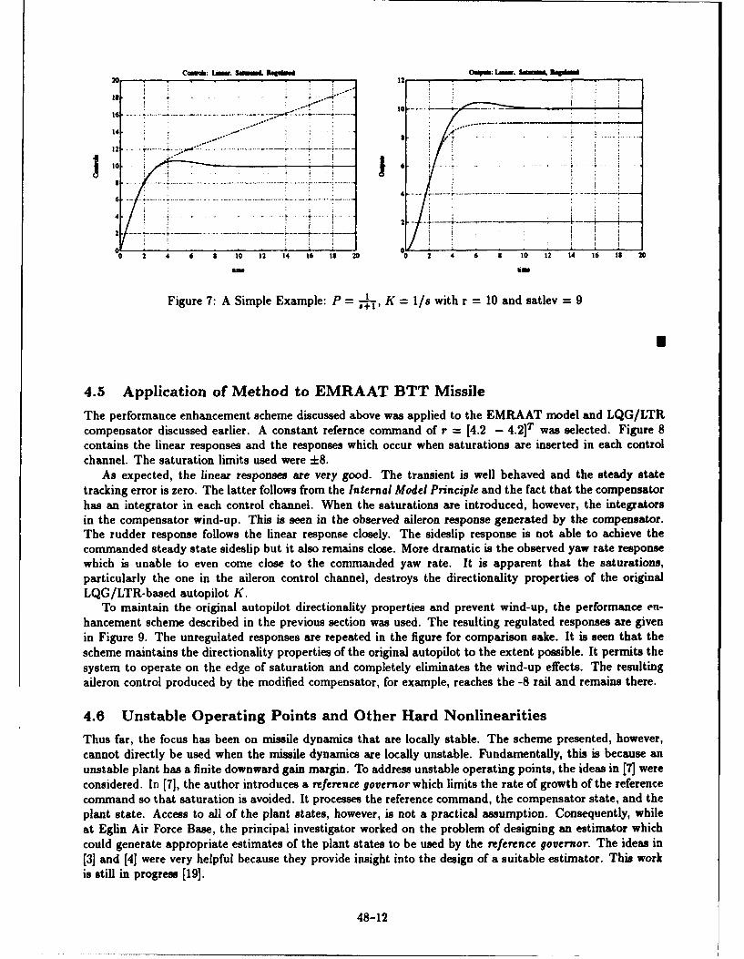
Cm Linin. 8damI.din n Ls. S oi. mmL s20 12 . •
If.C to ---16
14 -
. .. .. . .. .. .. .. ... . .. . . . ..... . . ...... ..
0 2 4 6 8 30 12 14 16 i8 20 0 2 4 6 1 t0 32 14 16 Is 20
im "N
Figure 7: A Simple Example: P K = 1/s with r = 10 and satlev = 9
4.5 Application of Method to EMRAAT BTT Missile
The performance enhancement scheme discussed above was applied to the EMRAAT model and LQG/LTRcompensator discussed earlier. A constant refernce command of r = [4.2 - 4 .2 ]T was selected. Figure 8contains the linear responses and the responses which occur when saturations are inserted in each controlchannel. The saturation limits used were ±8.
As expected, the linear responses are very good. The transient is well behaved and the steady statetracking error is zero. The latter follows from the Internal Model Principle and the fact that the compensatorhas an integrator in each control channel. When the saturations are introduced, however, the integratorsin the compensator wind-up. This is seen in the observed aileron response generated by the compensator.The rudder response follows the linear response closely. The sideslip response is not able to achieve thecommanded steady state sideslip but it also remains close. More dramatic is the observed yaw rate responsewhich is unable to even come close to the commanded yaw rate. It is apparent that the saturations,particularly the one in the aileron control channel, destroys the directionality properties of the originalLQG/LTR-based autopilot K.
To maintain the original autopilot directionality properties and prevent wind-up, the performance en-hancement scheme described in the previous section was used. The resulting regulated responses are givenin Figure 9. The unregulated responses are repeated in the figure for comparison sake. It is seen that thescheme maintains the directionality properties of the original autopilot to the extent possible. It permits thesystem to operate on the edge of saturation and completely eliminates the wind-up effects. The resultingaileron control produced by the modified compensator, for example, reaches the -8 rail and remains there.
4.6 Unstable Operating Points and Other Hard Nonlinearities
Thus far, the focus has been on missile dynamics that are locally stable. The scheme presented, however,cannot directly be used when the missile dynamics are locally unstable. Fundamentally, this is because anunstable plant has a finite downward gain margin. To address unstable operating points, the ideas in [71 wereconsidered. In [7], the author introduces a reference governor which limits the rate of growth of the referencecommand so that saturation is avoided. It processes the reference command, the compensator state, and theplant state. Access to all of the plant states, however, is not a practical assumption. Consequently, whileat Eglin Air Force Base, the principal investigator worked on the problem of designing an estimator which
could generate appropriate estimates of the plant states to be used by the reference governor. The ideas in[31 and (41 were very helpful because they provide insight into the design of a suitable estimator. This workis still in progress [19].
48-12
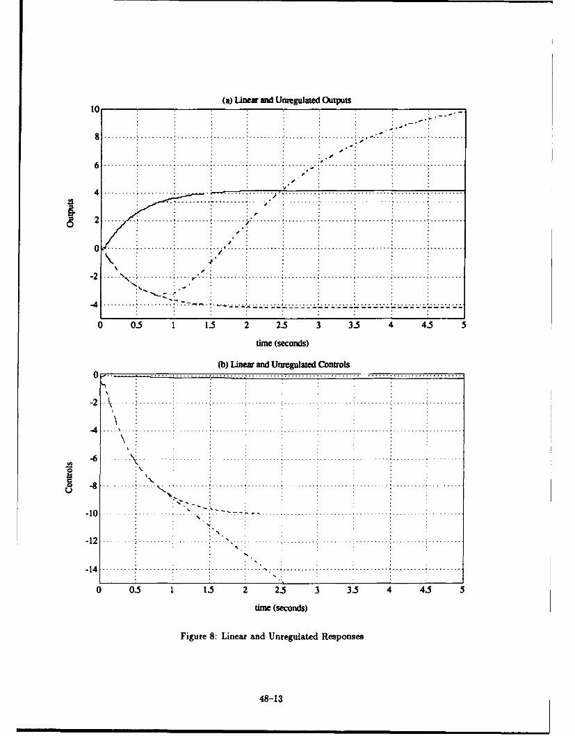
(a) Linear and Unregulated Outputs10
8 ... . . .. . . . . .. . . . .. . . . . .. .. ..6 - '. -°.-.
4 . . ..
7 . .. . . ..I .
4 . .. . . . . . . . ...... .. . . . . . . . . . .. . .... . . . . . . . .
0. .. . .. . . .. .. . . . . . . . . . ... . . . . . . .* ..... ...
0 .................. ..... ..., ... .. t. ...... :........ ., ..................... .................... .. . . .
-4 ~ . . . . . . . . . . . .. . . ... . . . . . . . . . . . . . . . . . .
0 0.5 1 1.5 2 2.3 3 3.5 4 4.5 5
time (seconds)
(b) Linear and Unregulated Controls
02 ... .
-4............................ ........ ...... .......... . . ...
. • _ .. "
-1 2 .. . ..... . .. . . .- - -
-14 .... ............... ......... .....N........ ..........
-14 ................... •2 '..-. . .. ., : .,:•................... ....................................... . . . . .
0 0.5 1 1.5 2 2.5 3 3.5 4 4.5 5
tfie (seconds)
Figure 8: Linear and Unregulated Responses
48-13
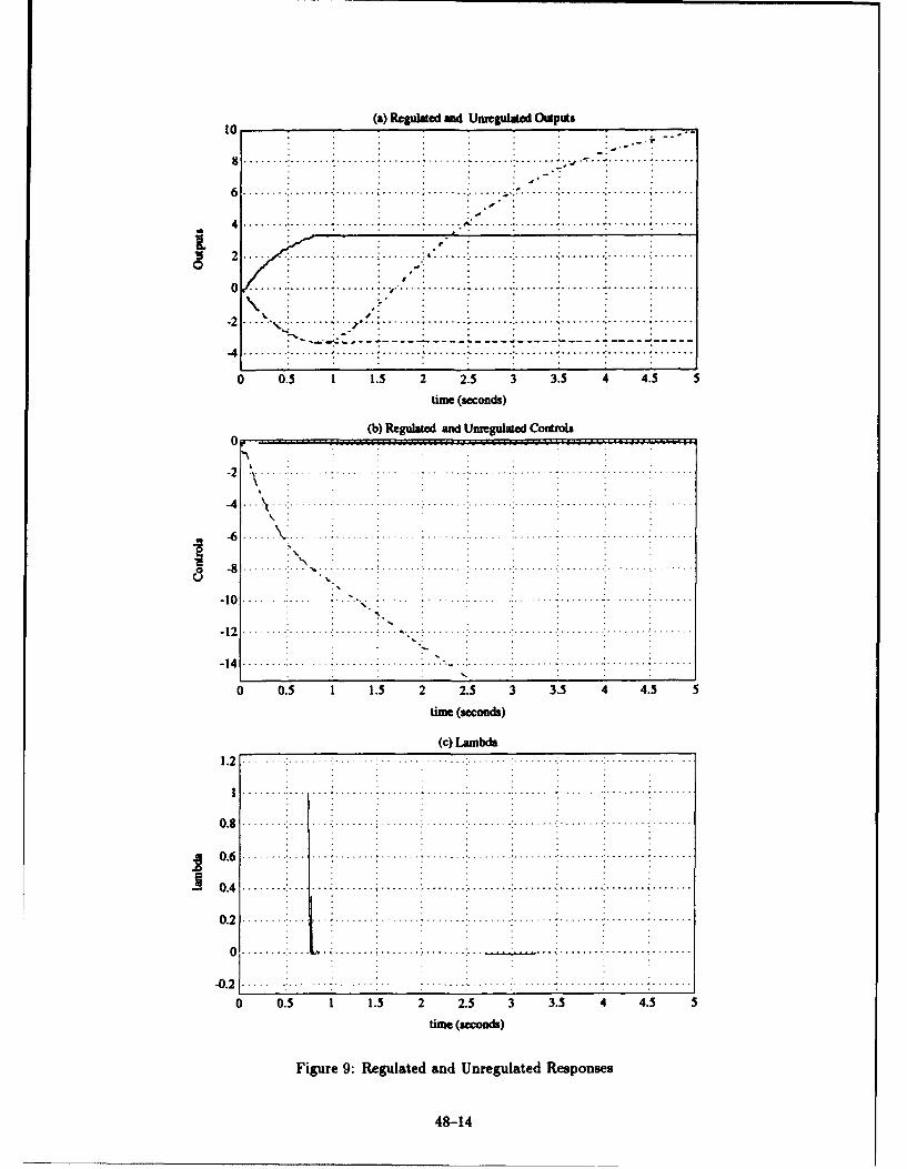
(a) Regulaed and Unregulated Outputs
.. . .. . .. . .. ..... . .... . . . . . _.. .. -
4 ....... .......... ......... .... . . . . .10
0 . . . . . . . . . . . . . . .:. . . . . . . . . ........ . ... .. . . . ,, - . . . . . .• . . . . . . . .• . . . . . . .• . . . . . ..2 ... ........ . .. ......
-4 ........ i ....... ".........,...... ....... ?....... !. . . .". . . .". . . .". . . .I J
0 0.5 1 1.5 2 2.5 3 3.5 4 4.5 5
time (seconds)
(b) Regulated and Unregulated Controls
-2 . . ..
-4 . .- :... . . . . . . . . . . . . :. . . . . . . :.. . . . . . . . . . . . . . . . . . . . . . . . . . . . . . . .. . . . . . .. . . . . . . .
-6 .. . .. V . ..... ..... .. . .. ............ . . .. ........... ... . .. .. ...... ..
, -8 . . . . . . . . -: .. . . . ... . .. . . . .. . . . . ... .. . .. . ... . . . . . .... . . . ... ... . . . . . . : . . .. . . .
* ... . . . . . . . .. . . . . . . .. . . . .
-114-'"- 1 . . . . . . . .. . . . . . ..: . . . .. . . . . . . . . .. : . . . . . . ... . . . . . . ... . . . . . . . . . . . . ... . . . . . . . . . . . . ..
-1 42 . . ... . ..* . . . . . . . . . . . . . . . . . . . . .. . . . . . . . . . .-14 . .. ... .. .. : . .. .. i ... ... : ..".. . ... . .. . ... ... . .. ................ .. ...
0 0.5 1 1.5 2 2.5 3 3.5 4 4.5 5
tue (seconds)
(c) Lambda
1.2 ................
I.. .......................
0.8 ........... .... ... ......
0.6. . . . ......... .. ....... .
:• 0 .6 -- ---... ... ......... ....... ................. ....... ......... . . . . .. . . . . . ..
S0 .4 ........ : ... ............ ........ ;.......: ........ :. ........ ........ ....... .......
02 .... .... . .
0 .. . . .. . . . . . . . .. . . . . -.-.-. . .. . . . . . .. . .. . . .
-0 .21 ............. ....... ..... .. .... .... . .. ......
0 0.5 1 1.5 2 2.5 3 3.5 4 4.5 5
time (seconds)
Figure 9: Regulated and Unregulated Responses
48-14

Other hard nonlinearities, such as rate limiters and a limiters, can be addressed using the methodsdiscussed thus far.
4.7 More General Nominal Compensation Schemes
The focus, thus far, has been on linear systems and, in particular, on nominal autopilots which are linear.It is clear, however, that nonlinear autopilots can be addressed using analogous ideas. The concept of a gfunction, for example, can be extended to the nonlinear case. Lets see how this extension might be done.
Suppose that K is a nonlinear £C finite-gain stable compensator with the following discrete-time repre-sentation:
X,+1 = f(z,.,e) (32)
Un = h(z,) (33)
Now one can define the zero input map as follows.
Definition 4.3 (Nonlinear Zero Input Map)Define the map from initial conditions z0 = z,,. to un as follows
Given this, it becomes apparent how to define the nonlinear version gNL of g.
Definition 4.4 (Nonlinear Version of g)Suppose zX E R". Given this, define the function gNL : Rn - R+ as follows:
lef9NL(Z) -e jI'f(r,n)lh:-
It is clear now, how to proceed with a nonlinear extension. Note, however, that gNL, unlike g, is notnecessarily positive homogeneous. This implies that, in general, gNL is not uniquely determined from itsvalues on the unit sphere. These ideas are currently under development. Extending the ideas to gain-scheduled autopilots where the scheduling variable is well behaved should also be achievable.
5 Significance of Work
The methods which have been developed in this research will systematize the design of full envelope con-trollers for missile systems with multiple hard nonlinearities. Systematizing the design process should signif-icantly reduce design time and lower system development costs. Preliminary results show clearly that themethods will increase system performance by permitting operation over the full envelope and in some casesextending this envelope. Finally, the methods developed will provide useful information to guide designersduring the initial stages of system development, design, and conceptualization. Given this, the contributionsof this research to missile control, and more globally to aerospace system development, should be significant.
6 Additional Collaborative Work
While at Eglin Air Force Base, the principal investigator initiated three collaborations.
6.1 Computation of Structured Singular Value Using Genetic Algorithms
The first collaboration took place with Professor Kamen Zhou of Louisiana State University and Mr. RichardHull of the University of Central Florida. This collaboration was initiated because of the need for effectivealgorithms for computing the structured singular value - a constrained spectral radius problem. This problemis important for determining the stability robustness, and more importantly, the performance robustness of"a missile autopilot with respect to structured uncertainty. This collaboration will result in the submittal of"a paper to the AIAA Guidance and Control Conference to be held in Phoenix, Arizona in August of 1994.
48-15

6.2 Performance Enhancement for Guidance Systems
The second collaboration took place with Professor Balakhrishnan of the University of Missouri-Rolla. Thiscollaboration was initiated because of the need for systematic procedures for designing integrated guidanceand control systems for missiles. Traditionally the guidance and control system have been designed separately.Our intention is to demonstrate how the performance enhancement methods discussed earlier can be usedto improve missile guidance. Our efforts have resulted in the submittal of a proposal for an invited sessionat the American Control Conference to be held in Baltimore, Maryland in June of 1994. A summary ofthe proposal has been included in the Appendix. Our efforts will also result in a submittal to the AIAAGuidance and Control Conference to be held in Phoenix, Arizona in August of 1994. The submittal will bea key component in a session which Professor Balakhrishnan and myself are organizing [?].
6.3 Extension to Gain-Scheduled Controllers
The third collaboration took place with Professor Jeff Shamma of the University of Texas-Austin. Thiscollaboration took place because of Professor Shamma's expertise in gain-scheduling and my interest inextending the methods presented above to general gain-scheduled controllers.
7 Summary & Directions for Future Research
During the course of this research, methods have been developed to facilitate the design of full envelopeautopilots for missiles with multiple hard nonlinearities. The focus, thus far, has been on maintainingperformance near a stable operating point in the presence of saturating actuators. The methods presentedmaintain to the extent possible the directionality properties of the original autopilot. They also eliminatewind-up effects and come with stability guarantees.
Future directions for research include applying the methods developed to a full six (6) degree-of-freedommodel for EMRAAT [(1 including the guidance and target dynamics. The ideas developed will be used toaddress unstable operating points and other hard nonlinearities such as rate limiters and a-limiters. Theideas also need to be completely extended to the nonlinear autopilot case and to the case where the autopilotis gain-scheduled [81-[9]. This will require the development of efficient methods for computing and analyticallymodelling the nonlinear version of g.
8 Bibliography
References
[1] I.A. Hirsch, M.A. Langehough, J.A. Bossi, et al. , "Advanced Robust Autopilot," Air Force ArmamentLaboratory, Eglin AFB, Florida, AFATL-TR-89-64, November 1989.
[2] J.H. Blakelock, Automatic Control of Aircraft and Missiles, 2nd Edition, John Wiley & Sons, Inc., 1991.
[3] B.A. Francis and K. Glover, "Bounded Peaking in the Optimal Linear Regulator with Cheap Control,"IEEE Transactions on Automatic Control, Vol. AC-23, No. 4, August 1978, pp. 608-617.
[4] H.J. Sussman and P.V. Kokotovic, "The Peaking Phenomenon and the Global Stabilization of NonlinearSystems," IEEE Transactions on Automatic Control, Vol. AC-36, No. 4, August 1991, pp. 424-440.
[5] E.G. Gilbert, and K.T. Tan, "Linear Systems with State and Control Constraints: The Theory andApplication of Maximal Output Admissible Sets," IEEE Trans Automatic Control, Vol AC-36, No. 9,September 1991, pp. 1008-1020.
[6] K.T. Tan and E.G. Gilbert, "Constraint Governors and Reference Constraint Governors for LinearDiscrete-time Systems with State and Control Constraints," submitted for publication in IEEE TransAutomatic Control, received October 1992.
[7] P. Kapasouris, "Design for Performance Enhancement in Feedback Control Systems with Multiple Sat-urating Nonlinearities," LIDS MIT, PhD Thesis, LIDS-TH-1757, March 1988.
48-16

[8] J.S. Shamma, "Analysis and Design of Gain Scheduled Control Systems," LIDS MIT, LIDS-TH-1770,PhD, May 1988.
[9] J.S. Shamxna and J.R. Cloutier, "A Linear Parameter Varying Approach to Gain Scheduled MissileAutopilot Design," Proceedings of the 1992 American Control Conference, Chicago, IL, June, 1992.
[10] C.A. Desoer and M. Vidyasagar, Feedback Systems: Input-Output Properties, Academic Press, Inc, NY,1975.
[11] J. C. Doyle, K. Glover, P.P. Khargonekar and B.A. Francis, "State-Space Solutions to Standard 72 and?io Control Problems," IEEE Trans AC, Vol 34, No 8, August 1989.
[12] A.A. Rodriguez and M.A. Dahleh, "71o Control of Stable Infinite-Dimensional Systems using Finite-Dimensional Techniques," submitted for publication in IEEE Transactions on Automatic Control, July,1993.
[13] A.A. Rodriguez and M.A. Dahleh, "Weighted ?'oo Optimization for Stable Infinite-Dimensional Sys-tems using Finite-Dimensional Techniques," Proceedings of the 29th IEEE Conference on Decision andControl, Honolulu, Hawaii, December 1990.
(14] A.A. Rodriguez, "Design of 71' Optimal Finite-Dimensional Controllers for Unstable Infinite-Dimensional Systems," submitted for publication to A UTOMATICA, August, 1993.
[15] A.A. Rodriguez and M.A. Dahleh, "On the Computation of Induced Norms for Non-Compact HankelOperators Arising From for Distributed Control Problems," Systems & Control Letters, December, 1992.
[16] A.A. Rodriguez and J.R. Cloutier, "Control of a Bank-to-Turn-Missile with Saturating Actuators",submitted for publication in the Proceedings of the 1994 American Control Conference, Baltimore, MD.
[17] A.A. Rodriguez and S.N. Balakrishnan, "Performance Enhancement for Missile Guidance and ControlSystems", proposal submitted for invited session to 1994 American Control Conference, Baltimore, MD.
[18] S.N. Balakrishnan and A.A. Rodriguez, "Performance Enhancement for Integrated Missile Guidanceand Control Systems", Invited Session, 1994 AIAA Guidance and Control Conference, Phoenix, AZ.
[19] A.A. Rodriguez and J.R. Cloutier, "Control of an Unstable Missile with Saturating Actuators", inpreparation, to be submitted to 1994 AIAA Guidance and Control Conference, Phoenix, AZ.
[20] M.G. Safanov, and M. Athans, "A Multiloop Generalization on the Cicle Stability Critrerion for Sta-bility," IEEE Transactions on Automatic Control, Vol. AC-26, No. 2, April 1981, pp. 415-422.
[21] G. Stein and M. Athans, "The LQG/LTR Procedure for Multivariable Feedback Control Design," IEEETransactions on Automatic Control, Vol. AC-32, No. 2, February 1987, pp. 105-114.
48-17

9 Appendix: Proposal for Invited Session to 1994 ACC
A.A. Rodriguez S.N. BalakrishnanArizona State University University of Missouri-RollaTempe, AZ 85287-7606 Rolla, MO 65401
Overview of Proposed Session
Because of the great uncertainty which an evasive target presents, the inherent nonlinear and typicallyunstable non-minimum phase dynamics associated with missiles, the integrated guidance and control ofmissile systems still represents one of the richest and most challenging control problems to the systems com-munity. During the past decade many advances have been made in the area of robust and nonlinear control.This includes results which facilitate the design of autopilots, provide insight into gain-scheduling, and allowengineers to better address nonlinear design issues. This session is an effort to bring researchers addressingvarious aspects of missile guidance and control together to present new results on enhancing the performanceof integrated missle guidance and control systems. The session is intended to shed light on some of the issueswhich researchers in the missile guidance and control community are now addressing.
Motivation and Summary
The title of the proposed session is
Performance Enhancement for Missile Guidance and Control Systems.
To properly address this subject, it is important that all aspects associated with missile guidance and controlare addressed. The organizers felt, for example, that it was necessary for the session to contain methods forsystematizing, optimizing, and enhancing the performance of today's autopilots and guidance systems. Thisincludes the issue of designing the autopilot to accommodate multiple hard nonlinearities such as saturatingactuators, rate limiters, etc. By so doing, autopilot performance would be enhanced and a much more flexibleguidance loop could be tolerated. Such a discussion must, however, involve a discussion of various autopilotdesign methodologies. For this reason, papers will be presented on autopilot design using eigenstructureassignment, 7X00-based methods, and the latest optimization techniques. The organizers also felt that it wasimportant for the session to contain new methods for improved guidance and target state tracking. This,it was felt could properly be addressed by researchers working on "approximately" analytical guidance lawsand nonlinear target state estimation algorithms which exploit the structure of the engagement and theestimator coordinate system.
To accomodate the above requirements, the organizers solicited papers from researchers in academia,industry, and the military. Six (6) papers were selected to address the following topics:
1. Performance Enhancement for a Missile with Multiple Hard Nonlinearities.A.A. Rodriguez, Ari7•i. a State University; Session Organizer.James R. Cloutier, - • nament Directorate, Eglin Air Force Base.title: Control of a Bank-to-Turn (BTT) Missile with Saturating Actuators
2. Improved Guidance Laws for Missiles: An Analytic Approach.S.N. Balakrishnan, University of Missouri-Rolla; Session Co-organizer.title: Improved Guidance Laws for Missiles: An Analytic Approach
48-18

3. Autopilot Design using N' Design Methods.
Kevin A. Wise, McDonnell Douglas Missile Systems Co.
Eric S. Hamby, McDonnell Douglas Missile Systems Co.
title: N'/ Missile Autopilot Design With and Without Imaginary Axis Zeros
4. Methods for Improved Target State Estimation.
Chris D'Souza, Armament Directorate, Eglin Air Force Base.
James R. Cloutier, Armament Directorate, Eglin Air Force Base.
title: Spherical-based Target State Estimation
5. Autopilot Optimization using Genetic Algorithms.
Richard Hull, University of Central Florida.
Roger W. Johnson, University of Central Florida.
title: Performance Enhancement of a Missile Autopilot via Genetic Algorithm Optimization Techniques
6. Missile Eigenstructure Assignment via Dynamic Compensation.
Robert Wilson, Armament Directorate, Eglin Air Force Base.
James R. Cloutier, Armament Directorate, Eglin Air Force Base.
title: Eigenstructure Assignment via Dynamic Compensation
48-19

A STUDY OF RAW DATA FUSION USING ARTIFICIAL NEURAL NETWORKS
Thaddeus A. RoppelAssociate Professor
Department of Electrcal Engineenng
Auburn UniversityAuburn. AL 36849
Final Report for:Summer Faculty Research Program
Wnght Laboratory
Sponsored by:Air Force Office of Scientific Research
Boiling Air Force Base, Wastungton. D.C.
September 1993
49-1

A STUDY OF RAW DATA FUSION USING ARTIFICIAL NEURAL NETWORKS
Thaddeus A. RoppelAssociate Professor
Department of Electrical EngineenngAuburn University
Abstract
A study of raw data fusion using neural networks was begun in Summer 1992. This is a continuation and
Ktension of that work. It is determined that target identification (classification) can be performed by a neural
etwork. For the particular data set that is used in these studies (the AADMS data set), identification based on IR data
,one is quite good. The neural network performance degrades when MMW and IR data are used (fusion). It has been
)und necessary to segment out the target-related MMW data from the rest of the data file as is done with the IR data.
At It is not clear that this can be done given the format of the AADMS data. Therefore. other data sets. including data
oni low-observable subsonic aircraft tower tests (LOSA) and some laser radar (LADAR) data have been processed
)r possible future use.
Details of the computer software and the data file file formats are provided. This software and data had to be
ansported on various media from their original sources, so the re-installation process was quite time - consuming,
id will be a continuing process for some time to come.
A comparison of neural network performance with classical approaches is made. Neural network operating
rinciples include many terms that we usually ascnbe to human behavior, including learning. instinct, intuition,
idgement, and confidence level. Like human performance, the accuracy of neural net performance is dependent upon
aining. With sufficient training, highly accurate responses are obtained at high speed.
Several ideas for commercialization and technology transfer utilizing neural network -based raw data fusion
•e proposed. including robotics, engine diagnostics, underwater detection, chemical analysis. voice processing, and
itomatic facial recognuton.
49-2

A STUDY OF RAW DATA FUSION USING ARTIFICIAL NEURAL NETWORKS
Thaddeus A. Roppel
I 0 Introduction
This report desccnbes work performed from 21 June 1993 to 10 September 1993 under the Summer Faculty Research
Progr _r (SFRP) at Wnght Laboratory. The laboratory focal point was Mr. Ellis Boudreaux in WL/MNG-X. This is
a continuation of work begun under the 1992 SFRP and continued in the interim under the 1993 Summer Research
Extension Program (SREP).
Previous work using the Westinghouse / AADMS data set demonstrated the capability to use a neural network to
tertorm sensor rusion for enhancing ground target identification. More specifically. medium-wave infrared (MWIR)
and millimeter-wave radar (MMW) data representing target scenes from AADMS were used to distinguish between
T-62 tanks. LANCE missile launchers. and M-I 13 armored personnel camers (APC's). The results from Summer
1992 are published in the 1992 SFRP Final Report. In summary. it was found that while IR data alone was sufficient
to correctly distinguish between the tank and launcher target images, a 14% improvement in confidence was obtained
by fusing the IR with the MMW data.
Further experiments on the AADMS data set subsequent to the 1992 summer program included using the leave-one-
out testing method to more realistically measure performance (described later in this report) , and adding the M-1 13
APC scenes to the testing matnx.
The new goals for the summer 1993 program were to investigate the inclusion of background non-target scenes in the
testing matrx. and to prepare some new data sets for analysis. The new data sets include the Low-Observable Sub-
sonic Aircraft (LOSA) data provided by IITRI-Huntsville. and some laser radar (LADAR) data from the ATLAS
program. Also under discussion is the possibility of obtaining medium- and long-wave IR data from the AADIOS
program from Integrated Sensors, Inc. (ISI). However, the AADIOS data has not been obtained as this report is
written.
Section 2 of this report describes the experimental methods used in the investigations. Section 3 is a presentation of
!he results. Section 4 is a discussion of the results, and Section 5 describes plans for continuing work.
49-3

20 Expennmental Methods
This section descnbes the basic neural network expenmental approach, the leave-one-out testing method. the ap-
proach to extracting background frames for testing, and the details of pre-processmg the new LOSA and LADAR data.
2 1 Neural Network Experimental Approach
The neural networks used in these expenments are simulated usir: ,ie ASPIRIN package distrbuted as freeware and
supported by MITRE In order to conduct an expenment. it is necessary to design the neural network architecture.
format the input training data for presentation to the network, initiate the neural network training, present the network
. sting data, and perform analysis of the results. As an example. the AADMS data fusion expenments use a
three-layer neural network with 228 inputs. 100 for IR pixels and 128 for MMW pixels. Each input is an 8-bit byte
rcpresentiie intensitv in the original pixel data file. but this is scaled to a floatng point value in the range from 0 05
Q) U '5 for presentation to the network inputs The network has 2 outputs. which also range from 0 05 to 0.95.
icpresentrie me confidence in the statements 'the input represents a Mnk," or "the input represents a misillunce."
The hidden laver consists of 20 nodes with sigmoidal activation functions.
The neural network is trained on 9 of the 14 available target scenes. The remaining 5 scenes are reserved for testing
the network Dunng training, the nine training scenes are presented repeatedly to the network while the back-
propagation of errors method is applied to adJust the internode weights. When the output error measures are suffi-
ciently low. training stops, and the network is considered to have learned the trairung data. In order to determine
whether the network has actually learned the difference between a tank and a launcher (rather than just having learned
about the specific tanks and launchers in the training set), we present the network with the five testing scenes held in
reserve, and measure the output error If the network correctly identifies these. then we say that the network has
performed a generalization of the training data.
The design of the neural network architecture is tightly coupled to the requred number of inputs and outputs. The
training time and memory requirements increase with the number of connections between nodes. An expenrment with
a few hundred inputs is tractable with desktop computing power. but processing a 128 x 128 byte IR image combined
with a large IM.W image is not realistic for anything except a supercomputer. Therefore. it is necessary to reduce the
amount of data presented to the network. Two techniques are combined to achieve this data reduction. First, the
tmage is segmented so that only the pixels in the neighborhood of the target are used. Second. the pixel count is
reduced by a neighborhood averaging process resulting in a 4-to- I reduction in each dimension for an overall 16-to-I
49-4

reduction. For the AADMS data. this resulted in a 10 x 10 pixel box surrounding each target. Although the segmen-
tation is presently being done manually, one future goal is to automate the target detection and segmentation using a
neural network.
Analysis of the results of training is performed by presenting the network with the testing data and measunng output
error relative to the ideal desired outputs. Several quantitative techniques are available, although the most commonly
employed is to use the rms error computed over all of the outputs nodes and all of the testing inputs. This provides a
single number which can be used to quantify the neural net performance. More detailed analyses, such as canonical
discriminate analysis (CDA) and principal component analysis (PCA), can be used to identify specific input images
that result in poor training performance and to optinuze the network architecture by correlating specific hidden layer
nodes with detection of unique features.
2 2 Leave-One-Out Trairnng
The training method used on the AADMS data provided results for a single arrangement of the available target scenes
into the two categories "testing" and "training." More generally, we would like to perform experiments using all
possible arrangements of the available data into these categories. While this approach would be thorough and ex-
haustive, in pracuce, a sufficient amount of information for most purposes can be obtained by conducting a subset of
these experiments. Namely, in leave-one-out training, all of the target scenes except one are used for training. The
left-out scene is used for testing. This is repeated until each target has been left out once. By accumulating the
resulting statistics, one obtains a very good picture of the overall performance of the network, as well as the effects
that can be traced to specific data files. For example, it often happens that certain inputs are "outliers," that is. they do
not represent the data space very well. perhaps due to excessive noise or obscuration. It is useful to identify these
outliers through leave-one-out experiments.
Leave-one-out experiments were performed on the AADMS data. One tank and one launcher image were simulta-
neously left out for each expenment. There were 10 tank scenes and 4 launcher scenes in the data set, so the number
of experiments was 10 x 4. For each of the 40 experiments. there were three possible outcomes:
(1) The target was correctly identified,
(2) The target was incorrectly identified.
(3) The target was not identified, i.e., the neural network output was undecided. or not
above threshold for either output.
49-5

By making a histogram of the number of times cases (1) - (3) occur dunng a set of 40 expenments. it is possible to
assign a performance measure to the neural network. These results are presented in Section 3. In addition. similar
experiments were run combining tanks and APC's, APC's and launchers. and finally all three vehicles. There were 8
APC target scenes available.
2.3 Background Scenes
All of thr ..- .rocessed to date consist of 10 x 10 pixel boxes approximately centered on targets. It is desirable to
generat. . . .. es that do not include targets. This provides an approach to training the neural network to perform
'arget aetecan by learning to distinguish between targets and non-targets. The success of this approach depends upon
the ability to span the entire space of non-target scenes with a relatively few number of background training scenes.
Background scenes a:e carefully chosen to include trees, ground. sky, buildings, and overlap regions.
2 4 Additional Data Sets
In addition to the AADMS data. the LOSA and LADAR data sets have been partially prepared for neural network
training. The LOSA data is MWIR and MMW data taken using essentially the same instrumentation as was used to
gather the AADMS data. The LADAR data was gathered using instrumentation implemented under the ATLAS
program at the Wnght Laboratory.
2.4 1 LOSA Data
The LOSA (Low-Observable Subsonic Aircraft) data set consists of tower data taken in late 1990 to early 1991 by
IITRI-Huntsville at the Army Missile Command in Huntsville. Alabama. This data set and some of the ground pro-
cessin, ) was provided by IITRI on several media. The raw data ti:c was provided on a 90MB Bernoulli
disk, the t., S was provided on 3-1/2" PC formatted diskettes, and the Maverick video was provided on standard VHS
videotape. In addition, a data catalog was provided on paper. The GPS was written in FORTRAN and Assembly
Language on a VAX /VMS computer. Since IITRI had archived all the files, it was necessary for them to de-arctuve
and extract the pertinent files before mailing them on their respective media. In this process. some of the files were
contaminated and/or transferred incomipletely, requirng some reconstructive work on both the data files and the pro-
gram files. In addition. the GPS program files were not written to be transportable. so a number of machine-dependent
modifications had to be made to the source code. The following subsections describe the LOSA data and program
49-6
files, the modifications. and the current state of usability.
24.1.1 Raw LOSA Data File, "RUNT06.DMS"
The raw LOSA data is stored in a 28.9 MB binary file with file name RUN06.DMS. This is the data from Run 6 of
Flight 6, as referenced in the data catalog entitled "DUAL MODE (MMW/R) DATA COLLECTION ON A LOW
OBSERVABLE SUBSONIC AIRCRAFr. DATA CATALOG. VOLUME I." This represents approximately three
minutes of data collected against a small airplane flying toward the tower, circling around, and flying outbound.
Dunng some of the time, the dual mode seeker is locked onto the target in tracking mode. Data frames are collected
at roughly 20 ms intervals and stored according to the format provided in the data catalog. The first few lines of the
data file are shown in Figure I for illustration.
When the file was delivered from IITRI and copied to the IPL VAX at Eglin. it was found to have a two-byte CR /LF
sequence inserted after every 512 byte block of the data. This was removed by using a C program entitled s2.c" to
rewrite the restored data file. This program is shown in Figure 2. The exact length of the data file is 29.941.824 bytes,
or 56.527 blocks of 512 bytes each. This file is processed by the GPS package to yield radar and IR map images which
are time-tagged to the Mavenck video. The user can choose a time of interest by viewing the videotape, and then
running the GPS software. The two major components of the GPS package are the data reduction subpackage and the
map processing subpackage.
2.4.1.2 LOSA Data Reduction Software Subpackage
This subpackage consists of the following programs:
REDUCES. FORFATDEF.MARGETFID.MARHEADER3.FOR
The purpose of this set of programs is to unpack the flight data and speed up the map generation processing. The call
to HEADER3 in REDUCES has been commented out. It seems that including this call would cause the data reduc-
tion process to stop at each slot and ask the user to make corrections to the slot header. The files FATDEF and
GETFID are assembly language code which perform low-level file access. A typical compile / link/execute sequence
utnder VMS with HEADER3 commented out follows.
%> FORTRAN REDUCE_S%> MACRO FATDEF. GETFID%> LINK REDUCES,FATDEF.GETFID
49-7

cheetah rappeil 13 od -vh run06.dmimsnor 000660 0000 0000 0000 0000 0000 0000 0000 0000
[OCTAL 0000700 000000000000(00000000000000000000
BYTE #1 0000720 0000 0000 0000 0000 0000 0000 0000 00000000000 0000000 l00 I b00 .500 0000 0 00000
0000740 00 000000 0000 0000 0000 0000 0000"0000020 000000000000000=0000000000000000
0000760 0000 0000 0000 0000 0000 0000 0000 000"0000040 000000000]0000000000000000000
0000060 0000 000 00000 0000 0000 0000 0000 0000
000000 000 ~ ~~00~ 333 ~[START BLOCK 2]
0001000 USe 42000030000000230 1000002000000000120 00000000000000000000000000000000
0001020 O00 0.00 3ce7 70e9g002 0dO2 bO&5 10000000140 0000 0000 0000 0000 0000 0000 0000 0000
0001040 0001 0100000000000000M000000000000000160 0000 0000 0000 0000 03000 0"0 0000 0000
0001060 00000000 0000000000000000000000000000200 000000000000 00000 0000 0000 0000
0001100 0000 00000000 00000000 0000 0000 0000000220 0000 0000 00000 0000000000000000000
0001120 000000000000000000000000 00000000000240 00000000 0000000000000000000000
0001140 0000000000000000000000000000 00000000260 00000000000000000000000 0000 0000
0001160 00003401 0301 d219 14el 80el f1le 00600000300 0000 0000 0000 0000 0000 0000 0000 0000
0001200 5c03 0000 0000 0000 0000 0000 0000 00000000320 00000000000000000000000000000000
0001220 000000000000000000"00000 000000o000340 0000000000000000000000000000 0000
0001240 0000000000000 0000 000 000 00000000360 0000 0000 0000 0000 0000 0000 0000 000
0001260 000000000000000000000000000000000000400 00000000000000000000000000000000
0001300 7200 7700 0000 00000000 0000 0000 6300"0000420 0000 0000 0000 0000 0000 0000 0000 O0O
0001320 00 0000 0100 0000 e000 0300 5018 00000000)440 00000000000000000000000000000000
0001340 0000 00000000000000000000000 00000000460 000000000000000000000000000 0000
0001360 00000 0000 0000 0000 cfV2 c4ff fc IS0000500 0000 0000 0 0"0" 0000 0000 0000O 00
0001400 0000 f4ff 8.16 816 9000 0800 0000 00000000520 00000000000000000000000000000000
0001420 000000000000000000000000 0000 00000000540 0000000003000000000000000000 0000
0001440 000000000000000000000000000000000000560 00000000000000000000000000000000
0000600 0000 0000 C)000 (XXX) (X ) 0 00000000001460 0000 0000 0000 0000 0000 00000000000
0001500 00000000000000000000000000000000"0000620 00000000000000000000000000000000
0001520 0000 0000 0000000000000 00000 0000"0000640 0000W00 00000 00000 0000000 000000
Figure I Hex dump of the first part of the data file RUNO6.DMS. The byte count is in octal. so 1000 represents512 bytes. The first block is a header for the file. The byte order within words is low byte-high byte. For
example. at the start of block 2. we have the system clock time recorded. It should be read as 0042ea88
hex Converting to decimal yields 4,385,416 hundredths of a second. Converting this to HH:MM:SS.ssyields 12:10:54.16, the clock time seen on the Mavenck video.
49-8

/* stnps off CR/LF from run06.dms */#include <stdio.h>#include <stdlib.h>FILE *fptrn, *fptrout,char InFileName([10, OutFileName[6];int ctr, dum. i;mainOIstrcpy(lnFileName, "run06.dms").strcpy(OutFileName, "s.out");fptrin=fopen(InFileName, "r"),fptrout=fopen(OutFileName, "w");while(dum!= EOF)Ictr= 1:while (ctr<513)
I
dum = getc(fptmn)putc(dum. fptrout);
ctr++.g
dumn = getc(fptnn);alum = getc(fptnin);
Ifclose(fptnn);fclose(fptrout).I
Figure 2. The C-program "s2.c" used to strip the CR/LFsequence out of the LOSA data file "run06.dns."
%> RUN REDUCE_S
Running this program results in the creation of four output files:
0006RUN06.IR (16,580,608 bytes) All the IR data0006RUN06.IQ ( 9,326,592 bytes) All the MMW data0006RUN06.KEY ( 3,294,720 bytes) All the status words0006RUN06.SEQ ( 203.264 bytes) Tape info and mode
transitions
These output files are used by the map generating software. The last slot of the file is slot number 5964 at time
12:13:31.99.
49-9
2.4.1.3 LOSA Map Generation Software Subpackage
This subpackage consists of the following programs:
DBSMAP.FORFINDTIM. FORPHASECO.FORPROMPTS. FORPROMPTS.INCSETWID.FORTAYLOR.FORTRACKFI.FORVAXLIB.OLBPLOTLIB .OLBFINDGAI.OBJ
The files PLOTLIB OLB and FINDGAI.OBJ are contaminated and have not been restored as of this writing. The
file VAXLIB.OLB was stnpped of extraneous CRILF sequences in a manner similar to RUN06.DMS. After com-
piling the FORTRAN programs in this list, a typical link and run sequence looks as follows:
%> LINK DBSMAP. FINDTIM. PHASECO. PROMPTS, SETWID. TAYLOR.TRACK_FI, VAXLIB.OLB/LIBRARY
%> RUN DBSMAP
Without FINDGAI. which computes the estimated gain imbalance between the I and Q channels of the radar data. it
is necessary to comment out the call in DBSMAP.FOR and set the vanable gainimbalance to 1.00. It is not clear at
present exactly how to handle the absence of the plotting library if plots are desired: this will be investigated further.
However, map files are still generated and can be used by other user-supplied graphics routnes. For example, it is
possible to view the IR maps using the KBV image-processing software on a SUN workstation. Running DBSMAP
with no plots requested results in the creation of the following files:
0006TIMES.06 list of dwell times processed0006xxxx. 06 IR maps. where xxxx are requested dwell numbers0006xxxx.m06 MMW maps
The MMW map files are generated in a call to scale mn,. DBSMAP. FOR. and this routine seems to be in the
plotting software which is not currently working. The IR fi... . saved in the form of a 19-byte header followed by
128 x 128 data bytes.
49-10

2.4.2 LADAR Data
The LADAR data was provided on a 44MB Bernoulli disk. The data files are descnbed in the data file catalog entitled
"IMAGE FILE FORMAT FOR Nd:YLF DATA STORED WITH YSAVE." Each data file contains intensity and
range data on scenes contining from one to six ground targets. For the purpose of viewing the intensity data using
KBV, the raw data files can be converted to KBV format using the following inputs to Forlmint. the KBV foreign
image conversion task: File Header = 4 bytes, Xsize = 256 bytes. Ysize = 1024 or 256 bytes (the actual file size for
each file is specified in the data catalog), Row Header = 512 bytes, Record Size = 256 bytes, and Record Header = 0.
The conversion of all the available LADAR data files to intensity images in KBV image file format has been per-
formed and the files are archived. In the future, we may extract the range data and use the range and intensity data
together in some data fusion experiments for target detection and/or identification.
2.4.3 AADIOS Dual Band IR Data
On 27 July 1993, Larry Nelson and Ed McDermott of Integrated Sensors. Inc. visited the Wright Lab and presented a
talk entitled "Raw Data Fusion, Status Review." ISI is under SBIR contract with the Air Force with Ellis Boudreaux
as the contract monitor. ISI presented results from several studies involving dual-band IR and video / IR fusion. The
dual-band IR data. which comes from the AADIOS program. will be transferred in the near future and used for neural
network sensor fusion experiments.
3.0 Results
This section summarizes results from the leave-one-out training, the background frame generation. and the preparation
of additional data for future experiments.
3.1 Leave-One-Out Training Results
The leave-one-out method was applied to the IR data from 14 target scenes prepared from the ADAMS data set. The
cumulative results are shown in the confusion matrx below.
It is clear that certain training/testing combinations lead to incorrect classification. Further detailed analysis and
explanation is presented in the report "Supervised Training in Artificial Neural Networks: Small Sample Size Meth-
odology for Selection and Analysis of Training Sets," wntten by Mark Townsley at Auburn University. 7his report is
available by making a request to Dr. Roppel. The gist of the above-referenced report is that two of the
49-11

Actual Classified As
Target Tank Launcher Undecided
Tank 23 11 6
Launcher 1 39 0
launchers and one of the tanks are recognized as conmibuting to all of the errors in classification. Visual inspection of
these specific target scenes shows that differences in ground shadowing is probably the main reason. When these
outliers are removed from the trairung data. performance improves considerably.
3.1 Leave-One-Out Fusion Results
A senes of experiments was conducted to measure neural network target identification performance using fused
MMW/IR data compared with using only IR data. The table which follows lists the various combinations of targets
for which the leave-one-out experiments were run. and the number of times each outcome occurred (* = correctly
identified. X = incorrectly identified. 0 = not identified). By comparing the IR-only results with the fused results in
the last row of the table, it is clear that the performance is degraded by the introduction of the MMW data. The reason
for this is that no attempt has yet been made to segment the MMW data as was done for the IR. Therefore, after the
MMW data is averaged down from 8 x 96 x 128 pixels to just 128 pixels, the number of pixels on the target is likely
to be significantly less than one. Thus. the radar data looks like noise to the neural network. The correct classification
percentage drops from 45% to 38%. while the incorrect classification percentage increases from 27% to 40%. The
same trend is observed for each row of the table, except for the first. Notably, this was the first combination on which
experiments were performed. which accounts for the overly optimistic performance evaluation based on the Summer
1992 results.
In addition to the leave-one-out experiments discussed above, both principal component analysis (PCA) and canonical
discriminant analysis (CDA) were performed on the results. A very readable discussion of these techniques is pre-
sented in "Analysis Tools for Neural Networks," by Simon Dennis and Steven Phillips. This paper is included with
the ASPIRIN version 6.0 release documentation, but a copy may be obtained by requesting it from Dr. Roppel. The
PCA techmque analyzes the dimensions in data space along which the network tnes to make maximum separation
between data items (e.g., target examples). CDA performs the complementary function of analyzing the clustering of
outputs performed by the network. The network after tratinng would ideally tightly cluster all targets of each kind,
49-12

IR only Fused MMW/IR* X 0 * 0 TOTAL
Tanks & Launchers 18 11 11 19 1I 10 40
Tanks & APC's 66 11 3 51 16 13 80
Launchers & APC's 17 9 6 13 12 " 32
Tanks. Launchers, & APC's 110 95 115 95 150 75 320
TOTAL 211 126 135 178 189 105 472
TOTAL % 45% 27% 29% 38% 40% 22% 100%
and maintain maximum separation between clusters. PCA and CDA were used on the fused tank / launcher AADMS
data. After training, the tanks and launchers were clearly sorted into two distinct, non-overlapping clusters, indicating
successful training.
3.2 Background Frames
One of the goals of this work is to investigate target detection in clutter and obscurauon. For this purpose. it is
necessary to uwn the network to distinguish between target and non-target images. Approximately 16 frames of
background scenery have been generated by extraction from the AADMS scene images. These will be used in future
experiments.
3.3 Results of Processing Additional Data Sets
In Section 2.4. the LOSA. LADAR. and AADIOS data sets are mentioned. Of these data sets, the most time was spent
on the LOSA data. The raw data files were obtained, the ground-processing software was refurbished and the entire
package was assembled and archived. The condition of the software is such that it is possible to generate IR map files.
but not MMW map files at this point. A little more work (perhaps a few days) is required to get the MMW plotting
capability online. The LADAR data has been transported to the SUN / Unix environment, and the IR intensity images
have been converted to KBV image file format. This data will also be archived.
4.0 Discussion
The purpose of this continuing investigation is to try to determine whether neural network technology might be suit-
able for eventual implementation in a dual-mode seeker. Conventional data handling approaches are based on
49-13

algorithmnc methods. which are in turn often based on Bayesian statistics and Gaussian noise assumptions. While
these assumptions are not strictly appropriate for every problem, many years of refinement have yielded good algo-
nthms. and so neural networks must perform very well in order to be considered advantageous.
The basic pnnciples underlying neural network performance are these: neural networks learn from "experience," i.e..
from available data: they provide fast. approximate solutions remmiscent of intuition and judgement calls in humans.
and they exhibit nch. complex "behavior" charactensuc of nonlinear dynamical systems. On the other hand, it is
difficult to trace the "reasoning" underlying a given response, and there is inherently a very difficult validation and
verification problem associated with neural networks.
Upon companng neural network approaches with algonthrmic methods we find the following distinction. Algonthmic
methods try to anticipate scenarios and encode them in rules to be followed at the time of engagement. Neural
networks, on the other hand. try to encounter scenarios in training, learn from them. and then respond "instinctvelv"
at the time of engagement.
It is well worth noting that both methods depend crucially on the quality and quantity of available data. In fact, it
might be appropnate to refer to the present situation in the field of target detection research as "algonthm-rich /
data-starved," (ARDS).
Looking ahead to possible hardware implementation. we find that the typical neural network chip architecture is
highly regular. resulting in high packing density, which in turn offers reduced pans count and weight. and increased
reliability. The neural network might be thought of as a computer program which is stored in the architecture of a
chip. Flexibility for modifications still exists at the layout and mask levels, however.
Distributed, redundant systems are generally highly desirable because they improve fault-tolerance and fault-
avoidance capability. Neural network-based systems have been shown to lean toward graceful degradation with in-
creasing input noise or when faced with intemal failures. The details of the failure response depend on the neural net
size and architecture details. A larger network will, in general. be more robust due to its increased redundancy. The
combination of fast response and high reliability is the primary motivation for studying the role that neural networks
might have in seeker technology.
49-14

The results thus far on the AADMS data. together with the results of other researchers. are encouraging. It is clearly
possible to train a neural net to perform target identification on a small scale. It is possible that by employing hardware
which is already available, a medium-scale mock-up could be developed and used for testing. It is important to pursue
this approach. since the true speed advantage of the neural net approach is not realized unless the network is imple-
mented in hardware.
It is considerably more difficult to make use of the raw MMW radar data than the IR data. Post-processing required
to get an image map is tremendous. so it is probably better to avoid this if possible. It should be feasible soon to fuse
the high-range resolution (HRR) profiles with the IR data. without having to perform pixel-to-pixel registration. With
regard to MMW/TR fusion, the two data types should be considered to be dissirmlar yet complementary. like audio
and video, rather than treated like dual-band IR, which is relauvely easy to pixel-register.
5.0 Plans for Continuing Work
One aspect of conunuing work that will be pursued is to try to get a more usable version of the AADMS MMW data.
The present version that is being used is the Doppler beam sharpened (DBS) processed data. However, there is
insufficient azimuth resolution to permut registration to any degree with the IR data. and there do not seem to be any
calibration markers in the data. John Watson of Nichols Research has indicated that it might be possible to de-archive
the original raw MMW data.
In addition to continuing the existing work for the Air Force, we are very interested in finding commercial applications
for sensor fusion technology. Technology transfer has been been identified as a prime goal for DOD, and we intend
to make every effort to continue thus work with that in mind. Several areas of possible application include robotics.
engine diagnostics, underwater detection. chemical analysis. voice processing, and automauc facial recognition. The
neural network approach is quite flexible relative to the types of sensor inputs that can be accommodated. For exam-
ple, a robotic application might use a combination of video. IR. and tactile inputs to identify machine parts. whereas
engine diagnosis aught involve a combination of audio and IR. inputs.
The LOSA data from IITRI will conunue to be processed. The software will be brought into as close to munt condition
as possible. and all of the relevant flight data will be extracted so that it can be used for MMW/IR fusion studies. The
dual-band IR AADIOS data will be obtained from ISI if at all possible. and this will be used for fusion experiments as
well. Finally, we propose to study the application of neural nets to a dual-band radar problem as proposed by Larry
Lewis at Wright Lab. This will require follow-tip after the end of the summer research period.
49-15

It is the intent of this author and his co-workers at Auburn to apply for follow-on research support in any capacity
where we can conmbute to the Air Force effort in multi-mode data processing and data / sensor fusion. It is of
particular interest to us to see that we maintain contact with everyone at the Wright Laboratory who has an application
or an interest involving neural nets and data fusion. The author encourages communication from interested individ-
uals, and can be reached at
(Internet) [email protected]
(Phone) (235) 844 - 1814
The End
49-16

THE AMIPLL PROGRAM FOR PREDICTINGP'ElVETRATOR BEHAVIOR ON IMPACT
William Keith RuleAssistant Professor
Department of Engineering Science and Mechanics
University of AlabamaBOX 870278
Tuscaloosa. AL 35487-0278
Final Report for.Summer Faculty Research Program
Wright Laboratory
Sponsored by:Air Force Office of Scientific Research
Boiling Air Force Base. Washington. D.C.
August 1993
50-1

THE AMPLL PROGRAM FOR PREDICTINGPENETRATOR BEHAVIOR ON IMPACT
William Keith RuleAssistant Professor
Department of Engineering Science and MechanicsUniversity of Alabama
Ahstruct
This report describes a computer program called AMPLL (Analytical Model for Penetration with
Lateral Loads). AMPLL is designed to predict the structural response of a penetrator passing through layers
of air, concrete, soil, ice, and/or rock. AMPLL is based on a similar program developed by Sandia National
Laboratories called SAMPLL. AMPLL differs from SAMPLL in that it has a mor,- extensive graphical user
interface and models the penetrator as a flexible body rather than a rigid body. Axial forces and lateral loads
due to angle of attack and impact angle are treated. The penetrator is modeled as a series of frame finite
elements, the number of which can be controlled by the user. Penetrators with arbitrary (but quasi-
axisymmetric) and varying cross sections can be modeled. Plastic behavior of the penetrator is treated in an
approximate fashion.
AMPLL is written in Microsoft Visual BASIC and runs on personal computers under Microsoft
Windows. The structure of the program ano how it can be used is described.
50-2

THE AMPLL PROGRAM FOR PREDICTINGPENETRATOR BEHAVIOR ON IMPACT
William Keith Rule
Jrdglarin
The development of a code called SAMPLL (Simplified Analytical Model of Penetration with
Lateral Loading) was initiated at Sandia National Laboratories in 1982 [1, 21. Development of this code
still continues. SAMPLL was designed to approximately predict the auitude and failure of penetrators
passing through layered targets of air. concrete, soil. ice, and/or rock. SAMPLL models the penetrator as a
rigid body and uses a unique concept of failure called excess impulse.
This project was initiated to enhance the user interface of SAMPLL, to model the penetrator as a
flexible body. and to provide a more classical, mechanics-based index of failure. The resulting program is
called AMPLL (Analytical Model of Penetration with Lateral Loading), is written in Microsoft Visual
BASIC, and runs under Microsoft Windows.
Instructions for running AMPLL are given in a section of this report entitled AMPLE User
Information.
Axial and Lateral Force Model
In general, a penetrator impacting a layered target will be subjected to both axial and lateral forces.
The empuircal axial and lateral force models used in AMPLL are essentially identical to those of SAMPLL
[1, 2]. Target layers of reinforced and unreinforced concrete, rock with horizontal bedding planes, isotropic
rock, soil. ice or frozen soil, and air can be treated.
The axial forces are predicted based on the assumption that a target layer will exert a constant
force, FA, on a decelerating penetrator. Equating the work done by the target on the penetrator to the initial
kinetic energy of the penetrator allows FA to be calculated:
WORK = KINETIC ENERGY
FAD =_MV2 (1)M-V22D
.FA..2
where: D is the depth of penetration into the target, M is the mass of the penetrator, and V is the initial
velocity of the penetrator. Thus, the axial force can be estimated if the depth of penetration. D, is known.
Empirical equations based on extensive testing have been developed to predict D [1,3]. Such equations
typically are of the form:
50-3

D = CISN(_W) f1(V,W) (2)
where: C, and C2 are empirical constants, S is the penetrability of the target, N is the nose performance
coefficient, W is the weight of the penetrator, A is the cross sectional area of the penetrator at the nose-body
interface, and f1(V,W) is a function of V and W which depends on the target type.
The penetrability, S. is used to allow for the characteristics of a particular target type within a class
of target types. For instance, nominal concrete would have an S of unity. and a high strength concrete could
have an S of 1. 1 or higher. The nose performance coefficient reflects the efficiency with which a particular
nose type penetrates and is given by equations of the form [1]:
N = f2 (LN,d) (3)
where: LN is the length of the nose, d is the diameter of the penetrator at the nose-body interface, and f2 is a
function of these parameters.
Axial loads are applied to the nose and to segments of the penetrator with a significant amount of
flare. It is assumed that a small amount of flare will not attract significant axial forces because the nose will
produce a slightly over-sized hole in the target. Axial l]--,As on the nose and flared sections are allocated in a
consistent manner to the finite elements making up these loaded segments.
Lateral loads are assumed to originate from two sources: angle of attack and penetrator angle.
Lateral forces affect the attitude of the penetrator as it passes through the layers. Lateral forces can also
produce large stresses in long penetrators due to bending.
Angle of attack, a, is the angle between the velocity vector and the axis of the penetrator. The
angle between the velocity vector and the target surface is called the impact angle, 0. The component of the
velocity vector perpendicular to the penetrator axis induces the lateral force. In effect, the penetrator is
impacting the target sideways. It is assumed that this type of lateral impact is similar in nature to axial
impact. Accordingly, the lateral force due to angle of attack is assumed to be proportional to the axial
pressure on the nose and to the angle of attack [1,2]:
F =C3( A .( (4)
where: C 3 is an empirical constant, and A, is the lateral projected area of an element. Note- a should always
be measured in radians.
When a penetrator enters a target a crater is formed. Similarly, as a penetrator leaves a layer, target
material often spalls off the bottom. Because of these effects, angle of attack lateral forces will tend to zero
50-4

when the penetrator is near the top and bottom of a layer. It is assumed that the target layer boundary
influence distance is 2.5C 4d, where C4 is an empirical coefficient (nominally unity) which can be adjusted
for different target types [2]. Thus. the angle of attack lateral force given by Eq. 4 is adjusted to vary
linearly to zero when the penetrator is within the boundary influence distance. The preceding remarks on
boundary influence effects applies to the case where the target layer under consideration is bounded by
softer layers or air. Adjacent layers of equal or greater hardness will not permit cratering or spalling so the
boundary influence correction need not be applied for these cases [21. The finite element model is used to
calculate axial and lateral nodal velocities. Thus, an angle of attack and lateral force can be determined for
each element.
Penetrator angle, 0, is the angle between the penetrator axis and the target surface. For normal
impacts, penetrator angle lateral forces are zero. However, during an oblique impact the target material on
the side of the nose closest to the surface tends to offer less resistance than the material on the bottom side
of the nose. Thus, there would be a net lateral force directed towards the surface. Similar effects would
occur as the penetrator approaches the bottom of the target layer. When the penetrator is relatively far from
the surfaces of a target layer then the impact forces on the top and bottom surfaces of the penetrator
approach each other and the penetrator angle lateral force tends to zero. This situation would occur in the
central portion of a relatively thick target layer.
The distance for which these layer surface effects are assumed to be active is 5C 5d, where C5 is an
empirical coefficient (nominally unity) which can be adjusted to account for different target types. Here
surface interaction distance is defined as the perpendicular distance from the penetrator centerline to the
layer surface. Penetrator angle lateral forces are only active where adjacent layers are softer than the layer
under consideration. It is assumed that cylindrical portions of the penetrator will not generate penetrator
angle lateral forces. However, flared sections will generate lateral forces in a manner similar to that of the
nose.
Penetrator angle lateral forces are assumed to be proportional to the axial force pressure on the
nose and the cosine of the penetrator angle [2]:
F, = C6( -A- cos(O)(C7 dToP - CsdBoTTOM) (5)
where: C6, C7, and C8 are empirical coefficients, and d'rop and dBOTTOM are the interaction distances to the
top and bottom of the layer, respectively.
50-5

Finite Element Mndel of Penetrator
One of the major tasks of this project was to convert the ngid body model of SAMPLL to a flexible
body model. This can be accomplished by modeling the penetrator as a series of plane frame finite elements
which can treat both axial and bending effects. Standard frame elements with a constant cross section were
adopted for this purpose [4]. Tapered elements could have been used but with no significant accuracy gain.
These elements have a node at each end with three degrees of freedom: axial displacements and forces,
lateral displacements and forces, and nodal rotations and moments. The stiffness matrix .-... ,ciated with
axial deformations and forces, [kJ,. is:
[k.]E e (6)Le L-1 1J
and that for flexural behavior. [kf], is:
12 6Le -12 6Le 1[k, • 6L 4L2 -6Le 2LMe (
S-12 -6%L 12 -6L)6Le 2L? -6Le 4Le 2
where: E is the e. modulus of the r.enetrator. 1. is the length of the element, A, is the cross sectional
area of the element it-length, and le is the flexural inertia of the element at mid-length. For example, a
penetrator with a tubtu -vs section of inside radius R1, and outside radius R,, has a cross sectional area
and an inertia given by:
Ae = n(R~ 2 -R) (8)
Equations 6 and 7 are assembled together in an appropriate fashion to produce a 6x6 elemental stiffness
matrix, [k].
A lumped elemental mass matrix. [me], which is diagonal, was used in the formulation [4]:
[m ]6.6= 1 1 17"5Le 1 1 (10)2 ( 210 210 (10)
where M, is the mass of the element. A fully populated consistent mass matrix could also be used which
might slightly improve the accuracy of the calculated results. However, lumped mass matrices have been
50-6

found to produce sufficiently accurate results and they have the advantage of being computationally cheap to
invert (inverted by simply taking the reciprocal of the diagonal elements - so matrix stays diagonal).
The global mass. [Ml. and stiffness, [K], matrices are created by assembling the elemental mass
and stiffness matrices in the usual fashion. The elemental mass matrices are diagonal. and so the global
mass matrix will also be diagonal and thus trivial to invert. The equation of motion can then be written:
[M]{i•}+[K]{x} = {FnPacz} (11)
where: { } are the nodal accelerations. { x} are the nodal displacements. and { Fn,,= } is an vector of
external axial and lateral impact loads which were discussed in the previous section. A damping term has
not been included in Eq. 11 since monolithic, high-strength metal components exhibit little damping.
Equation (11) can be solved for the nodal acceleration vector
{il = [M]'I[{ Fime}I-[K]{xl] (12)
Equation 12 shows that nodal accelerations are given by the inverse of the mass matrix multiplied into a
"delta force" vector which consists of the difference between the external impact forces applied to the
penetrator and the internal forces (= [K]{x}) in the penetrator. A scheme for approximately treating
plastic behavior is discussed below. Up to this point it has been assumed that the penetrator is behaving
elastically.A finite difference scheme is normally used to determine the new nodal displacements, {XNEW },
at the end of the next time step, AT, based on the acceleration vector of Eq. 12 and the current and previous
displacement vectors:
{ XN:w } - 2{xcupjtRE. } + {XpRvOUS 1(13
AT2 (13)
Rearranging gives [4]:
{XNE-j } = {X}CTR 4 xE.jN, }- {XPRVIoUs } (14)
The new velocity vector, {i w }, can now be calculated:
{XNEW - {XPREvIoUS2AT (15)
50-7

A global coordinate system is set up with the origin on the surface of the target where the nose will
first impact. A global x-axis is made to run parallel to the surface of the target and in a direction parallel to
the horizontal component of the penetrator velocity vector. A global z-axis runs from the surface of the
target and into the target. Most oblique impacts will cause the penetrator to rotate a considerable amount.
These rotations must be "factored" out of displacement, velocity, and acceleration vectors because the
components of these vectors must be precisely maintained either parallel or perpendicular to the axis of the
penetrator. Essentially, a local coordinate system must be made to travel with (or be in the frame of) thepenetrator. This is accomplished by rotating these vectors every time step by an angle AO, using the
following transformation matrix:
u } A os(AO) sin(Aý) 01'UT+AT1VT+AT -sin(AO) cos(Ap) 0/VT+AT (16)
0 T+AT L 0 0 1JIOT+AT J
where: u is the axial vector component, v is the lateral vector component, 0 is the rotational vector
component, and primed quantities refer to transformed quantities. AO is determined by the change in angle
of a line connecting the nose to the tail that occurs over a time step AT. Equation 16 shows no
transformation for rotational vector quantities, which is indeed the case for angular velocities and
accelerations. However, for the nodal rotations themselves the transformation is:
O-T+AT = eT+AT - AO (17)
The penetrator ang'e is also updated each time step:
' = + AO (18)
The impact load vector, {Fimlnt }, need not be corrected for penetrator rotations since it is always assumed
to be composed of components parallel or perpendicular to (as appropriate) the axis of the penetrator.
The penetrator is treated as a series of segments. Generally, each abrupt change in the geomeu'y of
the penetrator, such as a flared portion, is treated as a separate segment. The first segment is always the
nose. AMPLL is formatted to handle as many as 5 segments per penetrator. The user can select the number
of finite elements per segment to be used in the numerical model. Typically 4 or 5 elements are used persegment. Usually it is better to have a relatively uniform mesh density (number of elements per foot) and so
in some cases it may be a good practice to partition a long segment into two or more segments to attain a
more uniform mesh density.
50-8
The nose not very accurately modeled using beam finite elements because of its complex geometry
Generally. the cross section vanes considerably over the length of the nose. The software linearly
interpolates cross section areas, and flexural inertias based on the user input end point values for a
segment.. Thus, for modeling purposes it is recommended that the tip of the nose be given the following
area and inertia properties:
Ao = 2 ALN4 -- ALN (19)-"
10 = 2 1 LN -ILN (20)-i-
where subscripts indicate where the property is evaluated (-- is half the nose length). When linear
interpolation is applied to the tip values of Eqs. 19 and 20 then areas and inertias are precisely matched at
Sand LN. Alternatively, without a significant loss of accuracy. Ao and Io can be simply input as - ALN
and .-5 ILN, respectively. AMPLL does not monitor strain in the first j- of the nose for failure prediction
purposes because of probable inaccuracies in calculated strain values and uncertainties in the loading
distribution. In most cases these modeling inaccuracies are not important since the significant strains in the
penetrator are at midlength where the moments are largest.
There are two important, user-controUed parameters associated with the finite element model: the
number of elements used, and the size of the time step, AT. In general, accuracy improves as more elements
are used and the time step size is reduced. However, solution times increase dramatically as the model is
refined. The recommended approach is to use four elements per segment and the recommended time step
size initially, and then run the problem again using one or two more elements per segment with the
corresponding new recommended time step size. This approach is repeated until there is no significant
change in the calculated results, which indicates that the model has converged.
The recommended time step size is based on two considerations: the time required for an axial
elastic wave to pass through the shortest finite element, and the time required for the penetrator to pass
through the thinnest target layer. The time step must be made shorter (AMPLL uses Y20 of these times as
suggested in SAMPLL) than shortest of these two times if stable and accurate numerical results are to be
obtained. The axial wave speed is approximately equal to i ' where E is the elastic modulus and p is the
mass density. The axial wave transit time is defined as the length of the shortest element divided by the
axial wave speed. The layer transit time is defined as the thinnest target layer divided by the initial
penetrator velocity. AMPLL displays the recommended time step size and indicates which criterion governs
(penetrator or target).
Currently AMPLL assumes that the penetrator material is elasto-plastic. This means that the stress
versus strain plot is linear (G = EE)until the yield stress is reached and then it is assumed that the stress
50-9
stays equal to the yield stress as strain increases further. It is assumed that behavior in tension is idenucal to
that in compression. It is also assumed that failure occurs when strain levels reach a critical value of percent
elongation, which is a material property that must be measured and depends on the particular material a
penetrator is fabricated from.
Thus, the maximum axial force (either tension or compression) that can be generated by an
element is equal to OysAe and occurs when the cross section is fully yielded. AMPLL enforces
compatibility with this upper bound by replacing A, in Eq. 6 with an effective cross sectional area smaller
than A, when formulating the element stiffness matrix.
Similarly, an upper bound on the moment exists (called fully plastic moment, Mp) which occurs
when the compression stress block and the tensile stress block of the cross section are fully yielded [5].
AMPLL ensures that Mp is not exceeded by substituting the actual moment of inertia, i4. in Eq. 7 with an
appropriately smaller effective moment of inertia when formulating the element stiffness matrix. AMPLL
allows the penetrator to have arbitrary cross sections that are quasi-axisymmetric (evenly placed stringers
allowed) making determination of Mp for a given cross section difficult. However. most cross sections can,
to a sufficient degree of accuracy, be approximated as a tube. Accordingly, an effective tubular wall
thickness, t, can be calculated from:
0e 0JR Ae (21)
The compression and tension block forces are equal to ays(-) and they act at the centroids of e2ch half
of the cross section. The lines of action of these forces are separated by:
8(3RMtet-3Rot, +te)Ce =(22)3Ae
Finally, the fully plastic moment is:
Mp = ys5 (--)C = 4 32t-e-3Rot +t3e)
3 (23)
This simple approach to treating yielding appears to be adequate. However. since the finite element
model provides the strains in the penetrator, more sophisticated material models could be incorporated into
AMPLL.
50-10

Description of lrarnm Structure
AMPLL is written in Version 2 of Microsoft Visual BASIC (a sophisticated, object-oriented form
of the BASIC computer language) which generates programs that run on Intel chip based PCs (80386,
80486, 80586) under the Microsoft windows operating system. Users do not need a copy of the Visual
BASIC program to run AMPLL. AMPLL is composed of six fundamental types of files: code files
(lampll.bas, 2_ampU.bas), global variable file (global.bas), form files (mainmenu.frm, selrecrd.frm,
penemenu.frm, peneinfo.frm, targinfo.frm, impacond.frm, timestep.frlm, seloutptfrm, derecord.frm,
viewer.frm), data files (penetrat.txt, target.txt config.txt), output file (default name ampll.txt). and a scratch
file (ampLl.scr).
The code files contain the subprograms (subroutines) that perform the calculations and coordinate
program flow. Two code files are required to store all the subprograms of AMPLL because code files are
restricted in size to 64K. The global variable file specifies all global variables (variables that can be
accessed by all parts of the code) and also provides definitions of these variables. Each form file contains
information about a window that appears on the screen as AMPLL executes. Some calculations are
performed in the form files.
The penetrat.txt data file stores properties of penetrators, Table 1. AMPLL allows the user to select
penetrators from this file for making runs and to add newly defined penetrators to this file. Penetrators can
also be deleted from this file. Similarly, the target.txt data file stores information about targets, Table 2. A
complete run configuration (penetrator, target, impact and run parameters) is stored in the config.txt file to
expedite reruns under similar conditions, Table 3. The results of a run, along with an echo of the input data,
are optionally written to an output file with a user defined name. The data files and the output files are
ASCII files which may be inspected and modified independent of AMPLL using a text editor such as
Windows Notepad. While deleting records from penetraLtxt and target.txt a temporary scratch file,
ampll.scr, is opened. This file is automatically deleted during the run.
AMPLL program structure is displayed in Table 4. Subprogram main-program calls a series of
subprograms (set-model_parameters, setdefaults, etc.) which in turn call a series of subprograms, as
indicated by the arrows and columns in Table 4. How the form, data, and scratch files are used in AMPLL
is also indicated in Table 4.
AMPLL User Information
In this section the use of AMPLL will be described. First all the files on the program floppy disk
should be copied into a subdirectory of a hard disk. This copying is not essential, but will greatly speed up
program load time. If lack of disk space is a problem. then only files ampll.exe, grid.vbx, and vbrun200.dll
(0.51 MG of disk space) need be copied. If the computer has Visual BASIC Version 2 installed in it then the
50-11

last two of these files need not be copied. To get the program started, the user double clicks (with left button
of mouse) on ampll.exe under File Manager of Windows (or other Windows program starting techniques
could be employed). A header window then appears and the user has the option of clicking on start to
continue execution or clicking on stop to exit AMPLL.
Next the main menu window will appear which displays 10 options. An option may be selected by
double clicking on it or by clicking on it once to select it and then clicking on the continue command
button. Each option will now be described:
o Begin Impact Simulation - This option is selected to start the program after the user has completed all
data inputs. AMPLL then checks if all inputs are reasonable and begins the impact simulation. If some of
the inputs are not reasonable (a negative cross sectional area for instance) then a warning is issued and the
user is returned to the main menu window.
o Modify Current Penetrator or Select a New Penetrator - When this option is selected a new window
containing a combo box will appear. Clicking the down arrow button will display the option of modifying
the current penetrator and a listing of penetrators currently stored in the data file penetrat.txt. Clicking on a
penetrator in the list and clicking on continue will cause that penetrator to become the current penetator
and the main menu window will reappear. Clicking on the modify current penetrator option and then
continue will cause two windows to appear sequentially, prompting the user for data on the penetrator. New
data is entered by editing the default numbers in the white input boxes or by selecting from a combo box.
The user should click on continue when finished with editing the data in each window. After inputting the
data, the user will be given the option of storing the new penetrator in the penetrat.txt data file for later
reference.
o Modify Current Target or Select a New Target - This option is identical to that of the previous except
here targets are dealt with instead of penetrators. Previously stored targets are contained in data file
target.txt. Note that combo boxes are provided to select target layer types so the user will never have to type
in the layer type.
o Modify Impact Conditions - This window prompts the user for the initial penetrator velocity, the angle
of attack (nose up positive), and the impact angle, 0, which is the angle between the velocity vector and the
surface of the target.
50-12
o Modify Time Step Variable - Here a window pops open allowing the user to select the recommended
time step size (determined as described in a previous section) or to input another time step size. The user
must be sure to click on (and thus highlight) the time step to be used (recommended or user defined).
WARNING: Time step size should be reconsidered if the penetrator. the target, and/or the impact
conditions are modified. If the time step is too large then the numerical model could "blow-up" (numerical
values tend to ±00). If the time step is too small then unnecessarily long execution times will result.
o Modify Output/Element Options - This window prompts the user for a run title, the print frequency
(the number of iterations that must pass before the results are printed to the screen and stored in the output
file), the number of finite elements to be used per segment (same for all segments), and the point in the
penetrator (as measured from the tip of the nose) to monitor velocities, accelerations and so forth.
0 Read Previously Stored Configuration - This command will cause the previously stored configuration
(in file config.txt) to be read into AMPLL and become the current configuration. This includes penetrator.
target, and all other parameters associated with a run. Thus, after inputting this file the impact simulation
can be initiated without further input, or some aspects of the configuration can be modified before
calculations begin.
O Save Current Configuration - This choice will cause the current configuration (penetrator, target,
other run parameters) to be stored in file config.txt for later reference.
O Delete Penetrator Definition from Data File - Penetrators that are no longer of interest can be
removed from the data file penetraLtxt by selecting this option. The name of the penetrator to be removed is
simply selected from the combo box listing. A cancel button is provided to quit this command without
deleting a penetrator.
O Delete Target Derinition from Data File - This menu pick is identical to the previous one except that
deleting targets from the data file targettxt is the function.
0 Exit from AMPLL Program - This option will allow the user to exit form the AMPLL program
without performing any calculations.
Except for the first (begin simulation) and last (exit from AMPLL) choices in the main menu
described above, the user is returned to the main menu after executing an option. Thus, the usual approach
50-13

is to keep selecting menu options as required until the simulation has been defined to the user's satisfaction.
Generally, the time step size should be the last model parameter selected and the recomnmended value
should be used. It is good practice to save the configuration for future reference before beginning the
simulation.
Once the simulation has begun the screen will be filled with a single, main window displaying data
to help the user monitor, understand and visualize the solution. This window can be iconized by clicking the
down arrow in the upper right comer of the window. This will free up the screen for other tasks as AMPLL
executes in the background. Thus, productive work can continue on other applications as AMPLL runs.
AMPLL can be brought back to full screen size by double clicking on AMPLL's American flag icon.
The main window displays calculated results three ways. The upper right comer of the screen
contains a scrollable spread sheet displaying time. velocity, acceleration, and stress (at the point in
penetator specified by the user) as the program executes. The scoll bar can be used to scroll to any data
point during the run.
Below the spread sheet is a plot area for displaying velocity, acceleration, stress, 0 angle (angle
between penetrator axis and target surface), depth, and percent elongation as a function of time. Command
buttons are placed below the plot area to allow the user to select different plots as the program executes. The
type on the button becomes bold when selected. The color of the plotted line changes as the penetrator
passes from one layer to the next.
On the left and central portion of the screen is a to-scale (except for penetrator wall thickness)
drawing of the target layers and the penetrator cross section. The current deflected shape and position of the
penetrator is continuously updated on the screen as the simulation runs. Old penetrator positions are over-
written in light gray to provide a record of the trajectory. Continuously updated, color-coded, stress contours
are shown on the penetrator cross section. The stress levels corresponding to the contours are shown below
the drawing.
A hard copy (bit-mapped image) of the main display window can be obtained at any time by
clicking on the print command button in the bottom right comer of the screen. Better output can be obtained
if the printer is set to landscape mode (using Windows printer set-up). Also, the run can be halted at any
time by clicking on the exit command button in the lower right comer of the screen.
It is often of interest to observe the axial and lateral forces acting on the penetrator as the
simulation proceeds. A special window is available for this purpose that can be activated by pressing the
show forces command button on the bottom right side of the ,,.:reen. An adjacent hide forces button removes
the force display window from view. The force display window is movable and resizable for the users
convenience. The penetrator nose is on the left side of the window and the tail is on the right side. Vertical
50-14

dotted lines indicate element boundaries. Axial forces are shown in blue. and lateral forces in red. The
largest force displayed is shown in the window title box for reference.
When the simulation is finished a message will be displayed indicating why the simulation stopped
such as "Penetrator Passed Through All Target Layers". Then the user will be prompted for the name of a
file in which to store the simulation output if so desired. The user will then have the opportunity to scroll
through the data spread sheet, flip through the plotted data. and print out the display window. The run is
terminated by the user clicking the exit command button. The ASCII output file can be inspected using a
text editor such as Windows Notepad. can be inserted into a report in a word processing program such as
Word for Windows, or can be imported to a spreadsheet such as EXCEL for plotting.
Convergence Study Results
As more elements are used and as time steps are made shorter, the accuracy of the numerical
model should improve. In the limit (ignoring the effects of truncation errors), calculated results should
approach and converge to exact values. Thus, convergence is a necessary characteristic of a numerical
model if reliable results are to be produced. Accordingly, a convergence study was conducted using AMPLL
and the results are shown in Table 5. These results are for an typical penetrator (initial velocity = 2100 ft/s,
initial angle of attack a = 20, initial penetrator angle 0 = 780) passing through a concrete target. Table 5
shows that AMPLL results did not change significantly as the mesh was refined for the case considered.
Test Case Results
All the details of the test cases run can not be reported here because of the classified nature of the
results. However, some typical results are provided. The behavior of a small penetrator impacting a thick
unreinforced concrete target was predicted using AMPLL. The results are shown in Table 6 and they appear
to be reasonable. A large penetrator striking a thick unreinforced concrete target was also modeled using
AMPLL, Table 7. The results follow a rational trend.
Summary and Conclusions
The well known SAMPLL code for predicting penetrator damage and trajectory on impacting hard
targets was modified to produce a new code called AMPLL. The modifications consisted of:
"* A new interface to make data input easier and provide for visualization of calculated results as an aid to
checking the input data and understanding system behavior.
"* The rigid body model of SAMPLL was replaced by a flexible body model in AMPLL, which takes the
form of a finite element representation. This allows for more accurate predictions of stresses and strains
in the penetrator.
50-15

* A new. more classical approach to predicting penetrator yielding was developed.
As a result of this protect. the iollowingl cenclusions were reached:
"o The graphical user interface of AMPLL simplifies the task of data input and minimizes the chance for
errors.
"o Graphical display of calculated results by AMPLL helps the user understand the behavior of a
penetrator during impact.
"o The fnuite element model allows for a reasonably accurate prediction of the time history of stresses and
strains (including stress wave effects) in the penetrator.
"o AMPLL's limiting approach to modeling yielding appears to produce reasonable results.
"0 Further studies should be conducted to recalibrate the empirical coefficients derived from SAMPLL so
that they will be compatible with the flexible body model of AMPLL.
o Development of a more sophisticated scheme for treating yielding in the penetrator is desirable.
SnugreitionS for Future Work
It is suggested that the following four tasks be conducted to enhance the reliability of AMPLL:
1. Gather together (and make readily accessible) a set (or sets) of high quality, and pertinent impact test
results to serve as "official" benchmarks for computer code calibration.
2. Repeatedly run AMPLL adjusting the empirical coefficients slightly (increase a small percentage and
decrease a small percentage) to determine the sensitivity of calculated results to these coefficients.
Sensitivity curves could be fit through this data for each empirical coefficient to show change in
calculated result (say - final velocity) versus percentage change in empirical coefficient.
3. Input the sensitivity curves and the test data set into a nonlinear optimization program to determine
changes to be made to the empirical coefficients to minimize the difference (in a least squares sense)
between AMPLL calculated results and the official benchmark experimental results.
4. Enhance the approach for modeling yielding in the penetrator to allow for non-elasto-plastic materials
(could input stress-strain curve directly) and elastic unloading with residual plastic strain.
Re[ereneg
1. Young, C. W. and Young, E. R., "Simplified Analytical Model of Penetration with Lateral Loading,"Sandia National Laboratories, SAND84 - 1635, May, 1985.
2. Young. C. W.. "Simplified Analytical Model of Penetration with Lateral Loading (SAMPLL) - AnUpdate," Sandia National Laboratories, SAND91 - 2175. February. 1992.
3. Young. C. W. "Depth Prediction for Earth-Penetrating Projectiles," J. of the Soil Mechanics andFoundations Division, ASCE, 95(SM3). S03 - 817, 1969.
50-16

4. Cook, R. D., Malkus, D. S., and Plesha. M. E., "Concepts and Applications of Finite ElementAnalysis," John Wiley and Sons, New York, 1989.
5. Cook. R. D. and Young, W. C. "Advanced Mechanics of Materials," Macmillan Publishing Company,New York, 1985.
50-17

Table 1 Contents of penetraLuxt Data File.
pene-name$ PENETRATOR NAMEweight# PENETRATOR WEIGHTnumseg% NUMBER OF SEGMENTS IN PENETRATORseg.length#(i%) 43 numseg% of these records SEGMENT LENGTH
FORE END CROSS SECTIONAL AREA, INERTIA, OUTSIDE RADIUSsegarea#( 1, i%) seg_inertia#( 1, i%) seg.r#(l, i%) :2 numseg% of these records
AFT END CROSS SECTIONAL AREA, INERTIA, OUTSIDE RADIUSseg_area#(2. i%) seg-inertia#(2, i%) seg_r#(2, i%) :3 numseg% of r rt'Lurdsnose-typeS NOSE TYPE - OGIVE OR CONEyieldstress# YIELD STRESSe# ELASTIC MODULUSper-elong# PERCENT ELONGATION
Table 2 Contents or target.txt Data File
target-nameS TARGET NAMEnum-layers% NUMBER OF LAYERS IN TARGET
MATERIAL NUMBER, PENETRABILITY, THICKNESSmadl num%(i%) s#(i%) thick#(i%) *3 num layers% of these records
I
Table 3 Contents of config.txt Data File.
penenameSweight#numseg%seg-length#(i%) :: nurmseg% of these recordsseg.area#(1, i%) seg-inertia#(1, i%) seg_r#(I, i%) ¢C numseg% of these recordssegarea#(2, i%) seg_inertia#(2, i%) segr#(2, i%) 4- numseg% of these recordsnose-typeSyield-stress#e#per-elong#target-nameSnumjlayers%matl.num%(i%) s#(i%) thick#(i%) n num layers% of these recordsv# INITIAL IMPACT VELOCITYalpha# INITIAL ANGLE OF ATTACKbeta# INITIAL IMPACT ANGLEdt# TIME STEP SIZErun-titleS RUN TITLEprntfreq% ITERATION OUTPUT FREQUENCYel.per-seg% NUMBER OF FIN1TE ELEMENTS PER SEGMENTcalc_loc# LOCATION IN PENETRATOR FOR MONITORING STRESSES, VELOCITIES. ETC.
50-18
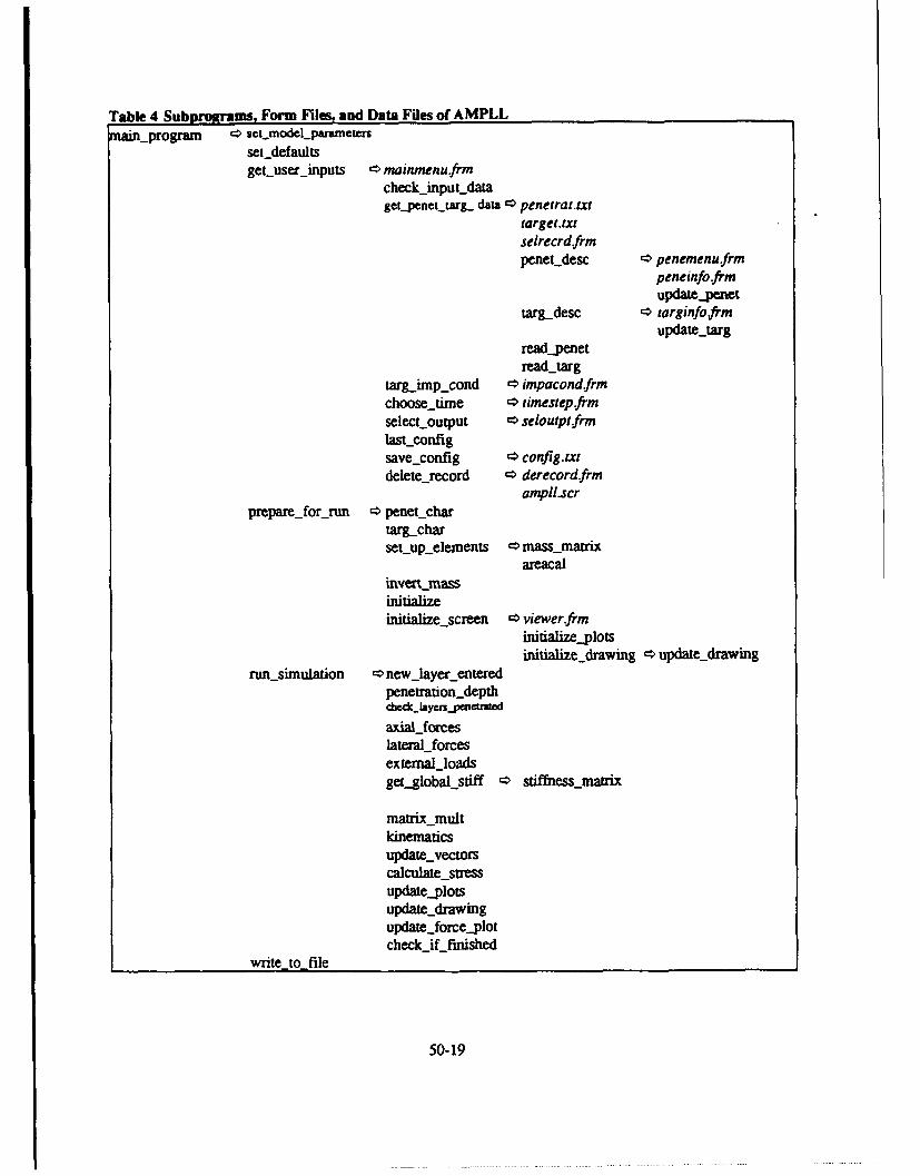
Table 4 Subprygmaus, Form Files, and Data Files of AMPLLMa.program c* set~modeI~parwnmetr
set-defaultsget-userjnput.s c mainmenu~frm
check_inpUt~dalagct-penet3ML.g data 'c' penetrat .txt
target .txtselrecrd~frmpenet-desc c* penemenu~frm
peneinfofirmupdate-.penet
targ-.desc c* torgmnfo-frmupdate jarg
rea&.penetread-targ
targ-imp~cond c* impacondfirmchoose-.time cý fimestepfirmselect~output seloutpt~frmlast~configsave -config config-tvdelete_record derecord~frm
ampll.scrpreparejforý-run c* penet-char
targ-.charset~up...elements c* mass_matrix
areacalinvert-massinitializeinitialize~screen ~'viewer frm
initialize~plotsinitialize...drawing c:, update,-drawing
run-simulation '>newjlayerý_entered
penetration..depthdbedcayer_.peneaulcd
axialjforceslateraljforcesexternaLloadsget-globat.stiff c* stiffness_mnatrix
matrix-multkinematicsupdate-vectorscalculate-suesupdate-..plotsupdatejirawingupdateJorce-..plot
write to file hcifiise
50-19

Table 5 AMPLL Convergence Study Results
Number of Time Step Size Final Velocity Final Penetrator Maximum Percent
Elements (ft/s) Angle (deg) Elongation
6 DEFAUL. 1853.7 72.86 1.19
12 DEFAU.i 1836.5 72.19 1.14
18 DEFAULT 1839.2 72.07 1.15
24 DEFAULT 1837.2 72.02 1.15
30 DEFAULT 1831.9 72.00 1.13
12 4xDEFAULT 1836.3 72.17 1.11
12 DEFAULT 1831,5 72.19 1.14
12 DEFAULT/4 1842.9 72.19 1.15
Table 6 Small Penetrator into Thick Concrete Target
hWt Velocity Init Penet Wit Ang of Final Vel Final Penet % Elong.(ft/s) Angle (deg) Attack (deg) (fMls) Angle (deg) (yield = .67)
2150 90 0 470 90.0 0.63
2150 77 13 <40 50.5 10.1
2650 90 0 1289 90.0 0.69
2650 87 3 1214 -9.7 3.17
Table 7 Large Penetrator into Thick Concrete Target
hit Velocity Init Penet Irit Ang of Final Vel Final Penet % Elong.
(ft/s) Angle (deg) Attack (deg) (ft/s) Angle (deg) (yield = .57)1900 88 0 1487 87.97 0.32
1900 86 2 1479 81.05 1.17
50-20

DEBRIS CLOUD MATERIAL CHARACTERIZATION FOR HYPERVELOCITY
IMPACTS OF MULTI-MATERIAL ROD PROJECTILES
Willian P. Schonberg
Associate Prfessor
Civil & Envirnmental Engireming Department
University of Alabama in Huntsville
Hun sville, Alabama 35899
Final Report for.
Summer Faculty Research Program
Wright Laboratory
Sponsored by:
Air Force Office of Scientific Research
Boiling Air Force Base, Washington, D.C.
September 1993
51-1

DEBRIS CLOUD MATERIAL CHARACTERIZATION FOR HYPERVELOCITYIMPACTS OF MULTI-MATERIAL ROD PROJECTILES
willa'm P. SchonbergAssoate Prfor
Civil & Envinnea Engineering DeparmentUniversity of Alabama in Huntsville
Huntsville, Alabama 35899
Abstract
In kinetic energy weapon impacts, one or more debris clouds are created during the perforation of a target
outer wall. These debris clouds expand as they move through target voids and eventually impact interior
components of the target. Depending on the engagemem conditions and the properties of the projectile and
target materials, these debris clouds can contain solid, melted, and vaporized material. To accurately
predict principle damage mechanisms and in turn the damage and break-up of targets engaged by kinetic
energy weapons. the percentages of debris cloud material in each of these three states of matter must bc
determined. This report presents a methodology to calculate 1) the amount of debris cloud material that is
solid, molten, and vaporous, 2) the debris cloud leading edge, trailing edge, center-of-mass, and expansion
velocities, and 3) the angular spread of the debris cloud material. The predictions of the method am
compared against empirically-based lethality assessment scheme predictions and against numerical and
experimental results.
51-2

DEBRIS CLOUD MATERIAL CHARACTERIZATION FOR HYPERVELOCITY
IMPACTS OF MULTI-MATERIAL PROJECTILES
William P. Schimberg, PhD
INTRODUCTION
The response of an aerospace target to a kinetic energy weapon (KEW) impact can be said to consist oftwo basic types: local response' and 'global response'. For KEW loadings, material damage associatedwith local response occurs very quickly (i.e. within the fim 30-40 psec) and is limited to a volume near theimpact location. Global response can refer to any one of a number of global phenomena that occur over alonger period of time, under less intense loads, and over a larger area of the target structure. In KEWimpacts, one or more debris clouds are created during the initial impact on the outer wall of a target. Thesedebris clouds expand rapidly as they propagate through target voids and eventually impact one or more in-terior components of the target. Depending on the impact velocity and the relative material properties ofthe projectile and target, these debris clouds can contain solid, melted, and vaporized material.
To accurately determine total target damage, a lethality assessment methodology (see, e.g. [1-3]) mustinclude the effects of discrete impacts by solid debris cloud fragments as well as impulsive loadings due tomolten and vaporous debris cloud material. Clearly, the amount of debris cloud material in each of thethree states of matter must be known to accurately assess total target damage and break-up due to a KEWimpact. This report presents a first-principles method to calculate I) the amount of material in a debriscloud created by a perforating hypervelocity impact that is solid, molten, and vaporous, 2) the debris cloudleading edge, trailing edge, center-of-mass, and expansion velocities, and 3) the angular spread of the debriscloud material. The method presented can be used for single- and multi-material solid rod projectilesimpacting an army of target plates. At this point, no adjustments have been made to account fordifferences in response due to projectile yaw or impact obliquity. The predictions of this methodology arecompared against those of empirically-based lethality assessment schemes as well as against numerical andempirical results obtained in previous studies of hypervelocity impact debris cloud formation.
SHOCK LOADING AND RELEASE ANALYSISIntroductory Comments
Consider the unyawed normal impact of a right circular cylindrical projectile on a thin flat target plate. Inthis study, the projectile is assumed to be made of one or more perfectly bonded dissimilar layers or disks.Upon impact, shock waves are set up in the projectile and target materials. As the shock waves propagate,the projectile and target materials are heated adiabatically and non-isentropically. The release of the shockpressures occurs isentropically through the action of rarefaction waves that are generated as the shockwaves interact with the free surfaces of the projectile and target. This process leaves the projectile andtarget materials in high energy states and can cause either or both to fragment, melt, or vaporize. Theresidual material energy is defined as the difference between the total energy of the material in the shockedstate and the energy recovered during the release process.
For the projectile and target geometries considered in this study, the shock waves are considered to beplanar. This simplification allows one-dimensional relationships to be used to predict the propagation,interaction, and release of shock pressures. The pressures, energies, and densities in the projectile andtarget materials after the passage of a shock are calculated using the three one-dimensional shock-jumpconditions, a linear relationship between the shock wave speed and particle velocity in each material, andcontinuity of pressure and velocity at all projectile and target interfaces. To calculate the release of theprojectile and target materials from their respective shocked states, an equation-of-state (EOS) is needed.
51-3

To keep the analysis relatively simple, the Tillotson EOS [4] was used in this study.
The Tillown Ea ution-of-State
In its original form, the Tillotson EOS has two parts. The first part applies when the material is incompression regardless of the internal energy (i.e. for V<Voand for all E>O) and in the =all region ofexpansion in which Vo<V<Vs provided that Es<E<Es'=Es+Hv where TV' is specific volume, Es is the totalenergy needed to produce incipient vapouization, and Hv is the latent heat of vaporization. The quantity Vscorresponds to the specific volume of a material that completes its release process with an internal energyE=Es. The second part apphies in a highly expanded state (i.e. for V>Vs regardless of internal energy) or ifthe internal energy is high enough to cause complete vaporization even in a moderately expanded state (i.e.for Vo<V<Vs and if E>Es).
In its two-part form, the Tillotson EOS is asymptotically correct in the compression and expansion regimesand is continuous across V=Vo for very high energy impacts. If we examine the two-part Tillotson EOS inmore detail, we note that at V=Vs, there is an abrupt jump in the release isentrope for moderate impactenergies, that is. when Es<E<Es. A modification in the form of a 'mixed phase formulation' of the Tdlot-son EOS was proposed to eliminate this abrupt discontinuity at V=Vs (see, e.g. (5,61). This modificationwas motivated by the fact that if Es<E<Es' as the isentrope crossed V=Vo, then sufficient energy would bepresent to cause only partial vaporization. Hence, the mixed phase formulation allows for some gaseousexpansion in moderately high energy impacts not possible with the original Tillotson EOS.
An alternative means of eliminating the discontinuity in T'dlotson EOS when V>Vs and Es<E<Es' is byuniformly subtracting the magnitude of the jump at V=Vs from the pressure values calculated when V>V,[7]. The amount of the jump in the release isentrope is largest if E=(Es)+ at V=Vs and decreases to zero asE--Es'. This jump correction is not intended to replace the mixed phase formulation of the Tillotson EOS,but rather to complement its use in the region V>Vs. In this report, the version of the Tillotson EOS inwhich the jump at V=Vs is eliminated by the uniform subtraction approach is referred to as theT'hlotson/SJC formulation while the mixed phase formulation of the T1lotson EOS is referred to as theTlllotson/MPF formulation. Unless otherwise specified, the Tilotson/SJC formulation was used in theremainder of this effort.
Pronapation of Shock Pressures in a Multi-Material Projectile
As the shock wave generated by the impact on the target propagates through the projectile, it encounters thevarious interfaces between material layers. At each interface between two dissimilar materials, atransmitted shock wave and a reflected wave are generated. The properties of the reflected and transmittedwaves ame found using a technique based on the method of impedance matching (see, e.g., [8-1 1]). In thistechnique, continuity of pressure and particle velocity are enforced at each interface. If the reflectedpressure is greater than the incident pressure, then the reflected wave is a shock wave. Conversely, if thereflected pressure is less than the incident pressure, the reflected wave is a rarefaction wave. An exampleof this technique is illustrated in Figure 1.
Figure 1, which consists of three Hugoniot curves drawn in pressure-particle velocity (P-up) space, showswhat happens when a shock wave traveling in copper at 12 km/sec encounters an aluminum interface.Using the three one-c&mensional shock jump conditions and the linear P-u relationship for copper, it isfound that a 12 km/sec shock wave in copper creates a pressure jump of T68 GPa and induces a particlevelocity of 5.34 km/sec in its wake as it moves into copper at ambient conditions. To find the pressuresand particle velocities of the reflected and transmitted waves, the Hugoniot for copper in P-up space isreflected about the point defined by up=5.34 km/sec, P=568 GPa. Its point of intersection with theHugoniot for aluminum yields the desired pressure (290 GPa) and particle velocity (7.15 km/sec) for thewave reflected back into the copper and tansmitted into the aluminum.
51-4

Once the pressure and the particle velocity in a subsequent material layer are determined, the one-dimensional shock-Jump conditions are used to calculate the specific volume and the energy of the shockedmaterial This procedure is repeated for each successive projectile material layer. Thus, while the impactconditions are used to define the shocked states in the target and first projectile layer materials, the shockedstates in subsequent pojectile material layers are obtained using the impedance matching technique justdescribed and illustrated.
Figure 1. P-Up Curves for Copper and Aluminum
2000 Aluminum18001600= Copper
• 1400 -(D1200.
100044: 800.
400 _
200
0 1 2 3 4 5 6 7 8 9 10Particle Velocity Up (km/sec)
Releaem of Shm*ri esnures
The target shock pressures are released by the action of the rarefaction wave that is created by thereflection of the shock wave in the target from the target rear free surface. This rarefaction wavepropagates through the target material and into the shocked projectile layer materials. In doing so, it alsoreleases the projectile-materials from their respective shocked states. For the purposes of the modeldeveloped herein, this process of shocking and releasing continues until the rarefaction wave overtakes theshock wave. After this point in time, it is assumed that no additional shocking and release of projectilematerial occurs. In this manner, the model considers only material that is "fully shocked".
As mentioned previously, in some instances the relative impedance of two adjoining projectile layermaterials may result in a shock wave being reflected back into a projectile material layer that has beenshocked and released. However, it is assumed for the purposes of this study that this reflected shock wavedoes not "re-shock" the projectile material and that the material into which it is reflected remains released.This assumption is reasonable since as the reflected shock wave moves back into the released layermaterial, it continuously creates rarefaction waves at the projectile edge free surfaces which release anymaterial shocking it produces. Thus, in the model developed herein, any projectile layer material that hasbeen shocked and released will remain released regardless of the nature of the wave reflected from itsinterface with an adjoining layer.
DEBRIS CLOUD MATERIAL CHARACTERIZATION
Computing the Percentages of Solid. Loquid. and Vaporous Dehres Cloud Material
Once the residual internal energies in the shocked and released portions of the projectile and target
51-5

materials am obtained, the percentages of the various states of mater in the resulting debris cloud areestimated& be procedure used requires knowledge of themaerials' solid and liquid specifc heats
,Cl) )their melting and boiling temperatures (TmTv), and their heats of fusion and vaporization(.v' naddition to the materials' internal residual energies (Er).
If Er<CpTm, then all of the shocked and released materials is considered to remain m a solid state. IfCPSTm-erTCpjm+Hf, then the quantity (Er-CesTm)/Hf represents the fraction of the shocked andreleased material that was melted, while the remaining shocked and released material is assumed to be insolid form. If CpTm+H f<Er< CpsTm+Hf+Cpl(Tv-Tm), then all of the shocked and released material isconsidered to be in a liquid state. If CnsTm+Hf+Cpg(rv-Tm)<Er< CpsTm+Hf+Cpl(Tv-Tm)+Hv, then thequantity (Er-[CDsTm+Hf+Cpl(Tv- Tm)])/Hv represents the fraction of the shocked and released materialthat is vaporized, while the remaining shocked and released material is assumed to be in liquid form. IfCpsTm+Hf+Cpl(Tv- Tm) +Hv<Er. then all of the shocked and released material is considered to bevaporized.
Computing the Masses of the Solid. Liouid. and Vanorous Dehris Cloud Material
To calculate the masses of the various states of the projectile and target materials in the debris cloud, theamounts of shocked and released target and projectile material need to be determined. These quantities areobtained by determining the locations in the target plate and in the projectile where the rarefaction wavesovertake the corresponding shock wave. These locations are found using a technique derived from thatused for single-material projectiles [ 12].
Figure 2 shows the results obtained when this technique is applied to a 3-layer projectile impacting analuminum plate at 6 km/sec. The projectile materials, their stacking sequence, and the geometry of theimpact are also given in Figure 2. As can be seen from Figure 2, the original rarefaction wave emanatingfrom the target rear surface overtakes the shock wave in the projectile at a distance of approximately 0.71cm from the leading edge of the undisturbed projectile. This implies that at the impact velocity considered.the fiat two projectile layers (i.e. the aluminum and the steel) are completely shocked and released as is thefirst 0.202 cm of the third projectile layer (i.e. the tungsten).
Figure 2. X-T Diagram for a 6 km/sec ImpactIALl <- IALISTIWI
0.06 A0.05 N.
"0.04 / N
0
N0
I-. 0.03 NN INE/\
IN
0. 1 INN
-0.4 -0.2 0 0.2 0.4 0.6 0.8 1 1.2 1.4 1.6
Axial Position X (cm)( =0.254 cm, LI = L2 = 0.254 cm, L3 =5.08 cm)
It is the material through which both the shock wave and the release wave travel that is shocked and re-
51-6

leased and which is therefore either melted or vaporized, depending on the impact velocity. Any materialbeyond the point at which the rarefaction wave overtakes the shock wave is assumed, for the purposes ofthis study, not to be shocked and to remain in a solid matter state. If the point at which the release waveovertake the shock wave is beyond the thickness of the target plate or the length of the projectile, then all ofthe target and/or projectile material is shocked and released. Thus, according to the assumptions anddefinitio presented herein, the remaining 0.306 cm of the tungsten layer in the projectile coresponding tothe impact depicted in Figure 2 is unshocked and unreleased.
In calculating the amount of target material subject to shock loading and release, it is assumed that theshocked target material comes from an area of the target equal to the presented area of the projectile [ 13];the remaining material ejected fron the target in the creation of the target plate hole is assumed to remain ina solid, albeit undoubtedly fragmented, state. Furthermore, it is also assumed that the depth of the shockedtarget material extends completely through the target thickness. Were this not the case, then other targetfailure modes, such as plugging, for example, might come into play. This in turn would seriouslycompromise the validity of the assumptions made in the development of this debris cloud model. A directconsequence of this assumption is that the model developed herein is not valid for "thick" target plates, i.e.those plates in which T/D>-0.75.
Once the projectile and target mass-contributions to the debris cloud and the fractions of these masses thatare shocked and released are obtained, the masses of the target and projectile materials in each of the threestates of matter are computed by multiplying each matter state percentage by the appropriate total shockedand released mass. The mass of the solid shocked and released material (if any) is then added to the massof the unshocked material (if any) to obtain the total mass of the solid material component.
A limitation of this procedure is the assumption that no further projectile loading and unloading occursbeyond the point where the release waves overtake the corresponding shock wave. This is not completelycorrect since the shock wave does not simply cease to exist once it is overtaken by a rarefaction wave.Rather, its magnitude decreases over a finite amount of time and a finite extent of material. Some addi-tional projectile material will be heated and possibly melted until the strength of the shock wave diminishesto a point below which melt no longer occurs.
DEBRIS CLOUD VELOCITY CHARACTERIZATION
Introductory Comments
In characterizing the velocities of the debris cloud created by a hypervelocity impact on a thin plate. thereare two possibilities that need to be considered. First, all of the projectile material is shocked and released.In this case, the debris cloud consists of the projectile and target material that is shocked and released andthe additional fragmented target material that is ejected from the target plate during the perforation processbut, according to the assumptions made herein, is not shocked and released. In the debris cloud modeldeveloped herein, all of this material is allowed to move axially and expand radially. The quantities ofinterest in this case are therefore the debris cloud leading edge, center-of-mass, trailing edge, and expansionvelocities, that is, vf, vi, vr, and Vexp, respectively. Second, some of the projectile material remains,according to the assumptions employed herein, unshocked. While it would not be appropriate to call thisunshocked projectile material a "residual projectile mass", it is reasonable to presume that this material isless severely stressed than that which is fully shocked and then released. Hence, it is also reasonable topresume that if there is any unshocked projectile material, then it does not significantly expand radially as itmoves axially. In this case, the debris cloud consists of shocked and released target and projectile materialsand the additional unshocked fragmented target material. The quantities of interest are the debris cloudleading edge, center-of-mass, and expansion velocities, that is, vf, vi, and vexp, respectively, and thevelocity of the remaining unshocked projectile material, Vpr. Note that due to the presence of theunshocked projectile mass, there is no debris cloud trailing edge for which to calculate a velocity.
51-7

It is noted that the equations developed in the subsequen secuom are presened in their umo general form.They can be apphed directly to a sungle-material projectile and adapted easily to apply to the impact of amulhi-material projectile.
In both of the cam described previously, the debris cloud leading edge velocity vf is approximated by Ufst,the velocity imparted to the target rear surface by the reflection of the target material shock wave. As in[ 14], ufst is taken to be equal to the sum of the particle velocity in the target material due to the passage ofthe shock wave, upt, and the particle velocity due to the passage of the nafaction wave in the targetmaterial, ut, created by the reflection of the shock wave from the target rear surface. Also common toboth cases is that the half-angle measuring the spread of the debris cloud material is given by
0= tawI(vexp/vi) (1)
What distinguishes the two types of debris clouds mathematically is the mainer in which vi, vUP and vr orvpr are calculated. When all of the projectile material is shocked and released, then:
Vr = vo- ufsp; (2)
vi is obtained from momentum conservation before and after the impact event, that is.
vi = mpvo/mdc; (3)
and. vexp is obtained from the application of energy conservation before and after the impact event, that is,
mpvo2/2 = Epr + E + mdcvi2/2 + mdevCXP2/2 (4)
where mdc- min+mt is the total debris cloud mass, mp is the projectile mass, mt is the total target hole-otmass, Epr and are the internal projectile and target energies, respectively, that have gone into heatingthe projectile and target materials, and ufsp=Upp+Urp is the velocity of the rear free surface of theprojectile. As in the case of ufst, ufsp is taken to be equal to the sum of the particle velocity in theprojectile material due to the passage of the shock wave, Upp. and the particle velocity due to the passage ofthe rarefaction wave in the projectile material. Urp, createdFby the reflection of the shock wave from theprojectile rear free surface.
In the event when not all of the projectile material is shocked and released, then vi, vexp, and Vpr amobtained through the solution of the following three simultaneous equations:
vexp = vf - vi; (5)
mpvo = mprvpr + mdevi; (6)
mpVo2/2 = Epr + Etr +mprvpr2/2 + mdcvi 2/2 + mdevexp2/2 (7)
where in this case mdr= mp+mt-mpr and mpr is the mass of the unshocked projectile material. If thesolution of the above system of equations results in a situation where there is insufficient energy availablefor debris cloud expansion or motion of the unshocked portion of the projectile material, then the leadingedge velocity is reduced until some kinetic energy does become available.
DEBRIS CLOUD CHARACTERIZATION SCHEME VALIDATION
Sinale-Material Proiectile
Comparison with Experimental Results and I-D Hydrocode Predictions
Debris cloud velocity values were calculated using DEBRIS3 (a FORTRAN77 program that implementsthe debris cloud characterization scheme developed herein) and compared against experimental results andone-dimensional hydrocode predictions obtained from a previous study of debris cloud formation and
51-8

growth using thin copper disks (LAD=0.3) impacting thin aluminum plates [14]. As can be seen in Table 1.the predictions of DEBRIS3 for vf, vi, and vr were in excellent agreement with those of the I -D hydrocodeand the expemental resuls
Table 1. C pmison of DEBRIS3 with Empircal Results and I -D Hydmcod Predict"V#oI # I' V' "rN ,4No
T p [ Vo (1) (2) 3) (1) 1 ('2) 1 (3) (I) (2) (3) (1) (3)(rm) (1) I
Effet a o T Thizdima1.0 1.0 6.39 1.44 1.41 1.40 0.91 0.89 0.89 0.36 0.34 0.34 0.24 0.27
1.5 1.0 6.36 1.44 1.41 1.40 0.91 0.83 0.84 0.36 0.34 0.34 0.24 0.322.0 1.0 6.38 1.42 1.41 1.40 0.83 0.79 0.79 0.35 0.34 0.34 0.27 0.362.5 1.0 6.53 1.46 1.41 1.40 0.79 0.76 0.79 0.35 0.34 0.33 0.27 0.36
1.5 1.0 3.45 1.34 1.39 1.39 0.76 0.74 0.74 0.43 0.36 0.36 0.23 0.331.5 1.0 4.45 1.43 1.40 1.39 0.37 0.34 0.84 0.39 0.35 0.35 0.23 0.33
1.5 1.0 6.36 1.44 3 .4 1 1.40 1 0.38 0.83 0.34 0.36 0.34 0.34 0.24 0.32
--fea -OPwieaik Man.2.0 1.0 6.38 1.41 1.41 1.40 0.83 0.79 0.79 0.35 1 0.34 0.34 0.27 0.362.9 3.0 5.66 1.44 1.40 1.40 0.82 0.80 0.79 - 0.34 0.34 0.23 0.364.4 10.0 5.12 1 1.40 1.40 1.39 0.33 1 0.80 0.79 0.36 0.35 0.35 0.22 0.37
(1) Experimental Results (14] (2) I-D Hydrocode Predictions (14] (3) DEBRIS3 Predictions
Over all the cases considered, the average difference between the predictions of DEBRIS3 for vf, vi, and vrand the corresponding experimental results was approximately 4% with a standard deviation ofapproximately 3%. However, the predictions of DEBRIS3 for Vexp exceeded the experimental results byan average of approximately 40% with a standard deviation of approximately 15%. This discrepancy mayhave been due to the fact that the expansion velocity measured in [14] was that of the heavier coppercomponent of the debris cloud while the expansion velocity calculated by DEBRIS3 was based on bothdebris cloud materials.
Comparison with CT'H and Lethality-Assessment Scheme Predictions
Figure 3 presents a comparison of the predictions of DEBRIS3, the hydrocode CTH [15], and the semi-empirical code FATEPEN2 [1] for debris cloud leading edge velocity vf for steel cylinders (L/D= 1)normally impacting thin aluminum target plates (T/D=0.125). As is evident in Figure 3, the predictions ofDEBRIS3 compare favorably with those of FATEPEN2 in the velocity regime for which FATEPEN2 wasdesigned to be used (i.e. less than approximately 5 to 6 km/sec). A quick calculation reveals that thedifference between the DEBRIS3 predictions of leading edge velocity and those of FATEPEN2 wasapproximately 26% of the DEBRIS3 values with a standard deviation of approximately 4% for the impactvelocities considered. One reason for this difference could be the fact that the mass of the impactingprojectile considered (approximately 1555 grains a 100 gms) exceeded the maximum value of projectilemasses used to develop the FATEPEN2 equations.
The CTH values plotted in Figure 3 are average values of the velocities of three Lagrangian station pointsalong the impact centerline within the aluminum target plate. These average values differed from thecorresponding minimum and maximum values by approximately 0.5 km/sec at an impact speed of 2 km/secand 3.0 km/sec at an impact speed of 14 km/sec. Inspection of Figure 3 also reveals that there is excellentagreement between the predictions of DEBRIS3 and cMH for debris cloud leading edge velocity. Theaverage difference between the DEBRIS3 and CTH values was approximately 4% of the DEBRIS3 values
51-9

with a standad deviation of apprximately 3%.
Figure 3. Debris Cloud Leading Edge Velocity ComponsonSteel Projectile (L/D= 1.0). Aluminum Plate (T/D=O.125)
25
w0 20.-_ __ _
'0---- DEBRIS3
Q 8 10- - CTH (avg)
n 5)>
0 0 I I II I I I
2 3 4 5 6 7 8 9 10 11 12 13 14 15 16Impact Velocity (km/sec)
Figure 4 presents a comparison of the predictions of DEBRIS3, CTH, FATEPEN2 [1], PEN4.v i0 [2], andKAPPI! (version 1.1) [3] for debris cloud half-angle for steel cylinders (L/D=1.0) normally impacting thinaluminum target plates (T/D=O.125).
Figure 4. Debris Cloud Half-Angle ComparisonsSteel Projectile (L/D= 1.0). Aluminum Plate (T/D=0. 125)
35-30
5 30"-- KAPPII/DAA02C
S25 -FTPN2/Steel0
go'--- FTPN2fAluminum_ 15
O -•- PEN4.vI0IA 10
1 -- DEBRIS3
02 3 4 5 6 7 8 9 10 11 12 13 14 15 16
Impact Velocity (km/sec)
In Figure 4, the average difference between the predictions of KAPPII and DEBRIS3 was approximately18% of the DEBRIS3 value with a standard deviation of approximately 10%; the average differencebetween PEN4.vlO and DEBRIS3 was approximately 6% with a standard deviation of nearly 7%. Based
51-10

on these results, it may be argued that the predictions of DEBRIS3 agree fairly well with those of KAPPIIand PEN4. However, comparing the differences between DEBRIS3 and FATEPEN2 was somewhat moredifficult because FATEPEN2 distinguishes between target debris spread and projectile debris spread whileDEBRIS3 does not. In FATEPEN2, the target debris half-angle is fixed at 250 while the projectile debrishalf-angle is based on material properties, impact conditions, etc.
It is interesting to note that unlike the smooth curve predictions of KAPPI, FATEPEN2, and PEN4, thecurve representing the growth of the debris cloud spread generated by DEBRIS3 contains numerous kinks.In particular, the impact velocities corresponding to the vertical lines in Figure 4 also correspond to impactvelocities at which significant changes occur in the way the initial kinetic energy of the projectile isdistributed to various competing mechanical and thermal processes during the impact evenL These featuresof the curve predicted by DEBRIS3 are discussed in the following paragraph.
For the impact considered in Figure 4, between 2 and 5 kn/sec, increasing the impact velocity resulted in asteady increase in debris cloud spread. However, at 5 km/see, the target material began to melt. As aresult, some of the additional kinetic energy of the initial impact provided as impact velocity increasedbeyond 5 km/sec was used up by the target material state change and was not available for debris cloudexpansion. Thus, the rate of debris cloud expansion slowed, and the slope of the curve decreased as impactvelocity increased beyond 5 kn/sec. Between 8 and 9 km/sec, the projectile material began to melt and thetarget material began to vaporize. This further decreased the rate of debris cloud expansion. However,once the projectile was completely melted, the rate of debris cloud expansion increased. Near 12 km/sec,the projectile material began to experience vaporization. The rate of debris cloud expansion slowed downonly slightly because by now the debris cloud consisted of a significant amount of hot vaporous material.By 15 km/sec. the debris cloud was nearly all vapor causing its rate of expansion to increase dramatically.
Multi-Material Projectiles
Introductory Comments
The validity of the multi-material modeling capability of DEBRIS3 was assessed by comparing thepredictions of DEBRIS3 against experimental and numerical data. The experimental data and the resultsof one series of hydrocode simulations were obtained from a study that analyzed the effectiveness oflayered projectiles against re-entry vehicle-type targets. The results of a second series of hydrocode runswere obtained using the CTH hydrocode specifically for the present investigation. The results of thisvalidation exercise are presented in the next three sections.
Comparison with Experimental Results
Three high speed impact tests were performed at 4 km/sec using three different equal-weight projectiles[16]. The first was a solid 7.5 gm TAIOW (i.e. a tantalum alloy with 10% tungsten) sphere, while thesecond and third projectiles were 7.5 gm layered spheres with a solid TA IOW core surrounded by a steelshell. The outer shell of the second projectile was 1018 steel (i.e. mild strength steel) while that of the thirdprojectile was 4340 steel (i.e. a high strength steel).
In simulating these three impact tests with DEBRIS3, the layered spheres were modeled as cylindricalprojectiles with three layers. The middle layer corresponded to the spherical core while the first and thirdlayers represented the outer shell material. The thicknesses of the first and third layer were set equal to theouter shell thickness. The thickness of the inner layer and the diameter of the cylindrical projectile werecalculated by setting the inner layer thickness equal to the cylindrical projectile diameter and then solvingfor the diameter by equating the mass of the cylindrical projectile to the mass of the original layered sphere.
In addition to adapting the geometry of the original projectiles used in the test series to a projectilegeometry that was compatible with DEBRIS3, some compromises were also made regarding the projectileand target materials. In the original test series, the target was a 2-D flat plate representation of a half-scale
51-11

re-entry vehicle. i.e. a layer of silica phenolic bonded to a thin layer of aluminum. Since the currnt versionof DEBRIS3 does not allow for multi-material targets. the targets used in the DEBRIS3 impact simulationsdid not have the outer layer of silica phenolic. In addition, while a witness block was placed behind theinitial multi-layer target plate in the experimental tests to record the damage of the perforating projectileand target debris, DEBRIS3 was not developed to have a predictive capatility for damage to subsequentwitness blocks or plates. Finally, whereas one of the original projectile materials was a tantalum alloy with10% tungsten, the corresponding material in the DEBRIS3 impact simulations was pure tantalum.
As expected, the simplifications described in the previous two paragraphs precluded any direct comparisonof the predictions of DEBRIS3 and the experimental results. However, it was possible to make qualitativecomparisons of the DEBRIS3 predictions and the actual test results because the simplifications maintainedsome similarity between the original test materials and configurations and the materials and geometries ofthe DEBRIS3 impact simulations. These qualitative comparisons became possible after the DEBRIS3predictions were analyzed to infer the relative severity of the damage levels that could have been expectedon subsequent witness plates had they been placed behind the initial target plate.
First. DEBRIS3 predicted that a significant portion of the target material would be melted when impactedby the solid tantalum sphere. Alternatively, when impacted by the layered projectiles, DEBRIS3 predictedthat the target material would be shocked and released but would return to a solid state of matter. Thisindicates that the target material would probably be fragmented but not melted. Second, DEBRIS3predicted that the kinetic energy of the remaining unshocked projectile material would be greatest for thelayered projectile with a tantalum core and a high-strength steel shell and would be least for the solidtantalum projectile. Taken together, these two features indicate that the cylindrical projectiles simulatingthe layered sphere projectiles would probably inflict morm severe damage on a wimess plate behind thetarget than would the cylindrical projectile simulating the solid TAIOW projectile. This agrees with theactual test results, which state that among the three impact tests, the crater depth and volume in the witnessblock behind the target impacted by the projectile with a TAIOW core and a 4340 steel shell were greatestand those in the block behind the target impacted by the solid TAIOW projectile were least.
Comparison with Hydrocode Predictions -- First Series
The first series of numerical runs consisted of Lwo sets of three high speed impacts at 11 km/sec using theSOIL hydrucode [161. The projectiles used were similar in construction to those in the previouslydiscussed experimental tests (i.e. one solid and two layered spheres in each test set). The majordistinguishing feature between the two sets of impact simulations in this series is the mass of the projectiles:45 gm projectiles were considered in the first set, while 5 gm projectiles were used in the second set. Inboth sets of simulations, the solid sphere was made out of tungsten as was the core in the layered spheres;the shells of the layered spheres were made out of different strength steels. In modeling the SOIL impactsimulations with DEBRIS3, simplifications in the projectile and target geometries were made similar tothose in the previous section. As a result, the following comparisons are again only qualitative in nature.
As in the DEBRIS3 simulations of the experimental tests, the DEBRIS3 simulations of the SOIL runsindicated that the solid projectiles would melt some of the target plate material whereas the layeredprojectiles would not. In addition, the kinetic energies of the unshocked projectile materials from thelayered projectiles greatly exceeded those of the unshocked projectile materials from the solid projectiles.These two features again indicate that the layered projectiles would inflict more severe damage on a witnessplate behind the target than would an equal-weight solid projectile.
Interestingly enough, while the general trends observed in the DEBRIS3 impact simulations agreed with thehypothesis that motivated the layered projectile investigation, they disagree with the actual numericalresults obtained as part of that investigation. The corresponding SOIL runs predicted that the witnessblock damage due to the impacts of the solid projectiles would be approximately the same as the damage
51-12

caused by the layered projectiles. Apparently, either the impact and/or geometric parameters used in theSOIL rum masked subtle differences in damage levels resulting from the solid and layered projectileimpacts and prevented them from being discernible, or the DEBRIS3 modeling of the projectile and targetgeometries over-emphasized some impact phenomenology that produced some differences in response thatwould otherwise have been negligible.
In any event, it is apparent that additional testing of multi-material projectile that are compatible with themodeling capabilities of DEBRIS3 are required to fully validate the predictive capabilities of DEBRIS3.As an intermediate step, several CTH runs were performed using projectile and target geometries that wereideally suited for and matched to the capabilities of DEBRIS3. The results of these runs and how theycompared with the predictions of DEBRIS3 are discussed in the next section.
Comparison with Hydrocode Predictions -- Second Series
In the second series of hydrocode runs, four high speed impact simulations were performed at 10 km/secusing CTH with multi-material cylindrical projectiles. The projectile diameter and target plate thicknesswere kept constant at 2.54 cm and 0.3175 cra, respectively. In the first two runs, the layers were relatively"thin" (i.e. LD=0.1 each), while in the seco d two runs, the projectile layers were relatively "thick" (i.e.L4)= 1.0 each). In the first and third runs, a a aluminum target plate was impacted by a projectile with analuminum leading layer, a 4340 steel middl: layer, and a tungsten rear layer. In the second and fourthruns, the order of the projectile materials was reversed. A detailed description of the impact and geometricparameters are given in Table 2; the results of the DEBRIS3 impact simulations and the correspondingCTH results are given in Table 3. In Tables 2 and 3, a '1' refers to the leading layer of the projectile whilea '3' refers to the rear-most projectile layer.
Table 2. Geometric and Impact Parameters for DEBRIS3 and CTH Comparison Runs
Run No.
(1) (2) (3) (4)
V (km/sec) 10.0 10.0 10.0 10.0
D (cm) 2.54 2.54 2.54 2.54
T (cm) 3.175 3.175 3.175 3.175
Target Material Aluminum Aluminum Aluminum Aluminum
Layer I Material Aluminum Tungsten Aluminum Tungsten
Layer 2 Material 4340 Steel 4340 Steel 4340 Steel 4340 Steel
Layer 3 Material Tungsten Aluminum Tungsten Aluminum
L1 (cm) 0.254 0.254 2.54 2.54
L2 (cm) 0.254 0.254 2.54 2.54
L3 (cm) 0.254 0.254 2.54 2.54
LID 0.3 0.3 3.0 3.0
Proj. Mass (gins) 38.24 38.24 382.40 382.40
The predictions of CTH and DEBRIS3 regarding the state of the target and projectile layer materials were
51-13

compared quantitatively and qualitatively. To facilitate quantitative comparisons of material end-states,average densities were computed for each material layer using the DEBRIS3 and CTH results. TheDEBRIS3 values were obtained by multiplying the mass of shocked and released material by its finaldensity, adding to it the product of the density of the unshocked material and its mass, and then dividing bythe total mass of the material layer under consideration. The CTH values are simply average valuesthrough the particular layer thickness and were obtained from density history plots along the centerine.
A feature common to all four impact simulations and evident in Table 3 is that the average target materialdensities predicted by DEBRIS3 were significantly higher than those predicted by CTH. However. thereason for this is that they include the solid component of target material not considered to be shocked andreleased by the impact (i.e. the remainder of the ejected target material not swept out u. .e projectile).The contributions of the solid material component to the average density of the target material amsignificant considering that they constitute approximately 90% of the target material in the debris cloudcreated by the impact. If the target hole diameter had been set equal to the projectile diameter (which is notan unreasonable assumption for the impact velocity and geometries considered), then there would not havebeen any unshocked target material and it is reasonable to presume that the average densities of the targetmaterial would have been much closer to the CTH values.
Table 3. Comparison of DEBRIS3 and CTH Impact Response Predictions
Run No.
(1) (2) (3) (4)
DEBRIS3 CTH DEBRIS3 CTH DEBRIS3 CTH DEBRIS3 CTH
vy 10.65 14.27 17.36 14.20 10.65 11.08 16.26 14.28(km/sec)
0 (deg) 36 32 34 27 48 37 21 22
Ptarst 2.56 0.21 2.36 -0.0 2.63 1.33 2.52 -0.0(gm/Cm 3)
P1 2.02 -0.0 18.52 0.67 2.22 2.25 18.98 9.20(gm/cm 3)
P2 7.04 0.17 7.25 5.50 7.83 8.53 7.83 6.94
(gm/cm 3)
P3 18.42 0.97 2.48 1.41 19.17 17.19 2.71 3.39(gm/m 3)
Debris Cloud Leading Edge Velocity and Half-Angle Spread Comparisons
The differences between the DEBRIS3 predictions of debris cloud leading edge velocity and thecorresponding CTH values in Runs No. 1-4 are 25.4%, 22.3%, 3.9%, and 13.9%. respectively, of the CTHvalues. The somewhat large differences in Runs No. 1 & 2 may be explained by the followingconsiderations. In the characterization scheme employed by DEBRIS3, the target shock loading andrelease analysis used to obtain the debris cloud leading edge velocity is truly one-dimensional. That is, it isperformed using only the leading projectile layer and the target material; anything behind the first projectilematerial layer is ignored. In the case of thick projectile layers. the use of one-dimensional equations isappropriate because the rear layers of the projectile are sufficiently far from the impact site so as not toaffect the magnitude of the velocity of the target rear free surface. However, in the case of the thin
51-14

projectile layers, the second and third projectile layers are close enough to the projectile-target interface toinfluence the shock and release process in the target material and the msuing velocity of the target rearfree surface. CTH, being a 3-D hydrocode, is apparently sensitive to these effects while DEBRIS3, beinga first principles code, is not. As a result, the CTH and the DEBRIS3 predictions differ somewhat mor inRuns No. I and 2 and are more in agreement in Runs No. 3 and 4.
The differences between the DEBRIS3 predictions of debris cloud leading edge velocity and thecorresponding CTH values in Runs No. 1-4 are 11%, 26%, 23%, and 5%, respectively, of the DEBRIS3values. The CTH predictions of debris cloud half-angle were obtained indirectly from debris cloud outputplots. In some cases, the precise angles were difficult to determine from the CTH plots because not all ofthe debris cloud material was retained by CTH and subsequently plotted. If there is a very small fraction ofa material in a cell in which more than one material is present, then it is possible for that small fraction ofmaterial to generate negative internal energies in that cell. CTH allows the user to set a flag that forcesCTH to drop the cell from subsequent calculations in such cases. If this is not done, then in such cases thetime-step becomes so small that the impact simulation will be forced to terminate prematurely. Apparently,in Runs No. 2 and 3, CTH dropped a fair amount of cells as the calculations proceeded which in turnproduced rather sparse debris clouds. While the agreement between the DEBRIS3 predictions and theCTH values was in general fairly reasonable, this may explain in part why in Runs No. 2 and 3 theDEBRIS3 predictions of the debris cloud half-angle values were significantly higher than the CTH values.Material Character~iation Comparisons* Proectiles with Thin Lay=r
Although Table 3 indicates that there were significant differences between the material densities predictedby DEBRIS3 and those obtained with CTH, closer examination of the DEBRIS3 and CTH predictions ofmaterial state did in fact reveal a qualitative agreement in the results.
For example, the extremely low material densities for Run No. I predicted by CTH indicate that thematerial from the three projectile layers in both cases are in highly expanded states. However, the densityof the rear-most portion of the third material layer in Run No. 1 (approximately the last 33%) was nearly3.5 times that of the forward portion of that layer, indicating that the rear third of the final projectile layerwas significantly more dense than the rest of the projectile material. Interestingly enough, for Run No. 1,DEBRIS3 predicted that the first two material layers would be in a liquid state, while the last 25% of thethird layer would not be fully shocked. Thus, while the actual density values may have been different(which was not totally unexpected given the relatively simple nature of the physics employed byDEBRIS3), there was some agreement between CTH and DEBRIS3 with regard to the state of theprojectile material following the initial impact.
With regard to the target material, CTH predicted that the target material would be in a highly expandedstate in Run No. 1 and probably vaporized in Run No. 2; DEBRIS3 predicted that the target materialwould be completely melted in Run No. I while in Run No. 2 it would be partially vaporized as well.Thus, there was again some general agreement between CTI and DEBRIS3 regarding the state of thetarget material following a hypervelocity impact.
Material Characterization Comparisons: Projectiles with Thick Layers
The projectile material characterizations predicted by DEBRIS3 were again found to agree in a generalsense with the post-impact material states predicted by CTH. For example, DEBRIS3 predicted that inboth Run No. 3 and Run No. 4 that the second and third projectile layers would remain unshocked whilepart of the first layer would be shocked and released. The CTH results for Runs No. 3 & 4 clearly showedthe third material layers to be relatively undisturbed and the second material layers to be only slightlydeformed. These characteristics are also evident in Table 3 where the density values predicted by CTH forthe second and third projectile material layers were near ambient values; the densities predicted by
51-15

DEBRIS3 for the second and third layers were naturally exactly equal to the respective ambient values due
to the assumptions within the DEBRIS3 model.
With regard to the first material layer, DEBRIS3 predicted that in Run No. 3 the entire shocked andreleased portim would be all liquid, whereas the shocked and released portion in Run No. 4 would be amixture of liquid and solid material. The CTH results for both cases showed that the density of the leadingedge of the first layer was approximately 30% of the ambient value, while the density of the rear portion ofthe leading layer approached the ambient value of the second layer material, indicating a significantly morecompressed state than that of the leading edge.
Some interesting features are also evident in the CTIH and DEBRIS3 predictions of the state of the targetmaterial. In Run No. 3. the average target material density as predicted by CTH is approximately 12% ofambient. This indicates a signficant liquid, if not vaporous, component of the target material in the debriscloud. For Run No. 3, DEBRIS3 predicted that 100% of the shocked and released target material would beliquid and that the density of the shocked and released target material would be approximately 75% ofambient. The near-zero value of the target material density as predicted by CTH in Run No. 4 indicates amaterial state near complete vaporization for the ejected target material while DEBRIS3 predicted thatapproximately 24% of the shocked and released target material would be in a vapor state and that 76%would be liquid. The density of the shocked and released target material predicted by DEBRIS3 was 40%of the ambient value indicating a highly expanded material state.
COMPARISON OF TILLOTSON EOS FORMULATIONS
Figure 5 illustrates the differences in the final specific volumes obtained in aluminum-on-aluminum impactsusing the Tillotson, T'illotson/SJC, and Tillotson/MPF EOS formulations and contrasts these with theresults obtained using the Mie-Gruneisen EOS [8]. For impact velocities below approximately 9 km/sec.the results were, as expected, nearly identical. For impact velocities above approximately 24 km/sec, thefinal values predicted by the Tillotson EOS and the two alternative formulations of the Tillotson EOSoverlap and significantly excteded those predicted by the Mie-Gruneisen EOS due to the gaseous expansionof the released material at those impact velocities.
Rgure 5. Aluminum-on-Aluminum Impact: Comparison of Rnal SpecificVolumes
21.81.6 1.4 Mie-Grunelsen
0. 1.4
> 1.- Tillotson
TIlotson/SJC
-0.- Tillotson/MPF,-r 0.4
0.20
4 6 8 10 12 14 16 18 20 22 24Impact Velocity (km/sec)
The odd behavior in the final values of specific volume due to the jump in the unmodified Tillotson EOS
51-16

began for aluminum-on-aluminum impacts at an impact velocity of approximately 9 km/sec. However, theTillotson/SJC formulation produced a smooth transition as the material changes from a solid state (belowapproximately 6 kin/sec) to a liquid state (between approximately 6 and 11 km/sec) to a gaseous state(above approximately 11 kin/sec). The specific volumes calculated by the Tillotson/MPF formulationclosely followed those of the Mie-Gnmeisen EOS until an impact velocity of approximately 18 km/secbeyond which they began to diverge rapidly. Apparently, the T1lotsor/SJC formulation predicted a moreexpanded material end-state than did the Tillotson/MIF formulation for impact velocities between 10 and24 km/sec.
Figures 6 and 7 compare the effects of using the Tillotson/SJC and the Tfllotson/MPF formulations,respectively, to calculate the percentages of the three matter states in debris clouds created by aluminum-on-aluminum impacts. While the results presented and discussed apply only to aluminum-on-aluminumimpacts, the equations developed herein may be used to estimate the state of the material within a debriscloud created by the high speed impact of virtually any two materials for which the required materialproperties are available.
Comparing Figures 6 and 7 reveals that the TIillotson/SJC and the Tillotson/MPF formulations agreed inthe percentages of the various states of matte r at speeds below approx. 11 km/sec and above approximately24 km/sec. Within the 11-24 km/sec impact ,elocity regime, the Tflllotson/MPF formulation predictedvaporization to develop more rapidly than did the T'illotson/SJC formulation which predicted a moregradual transition to vaporized material. This appears to contradict the results shown in Figure 5 in whichthe Tillotson/MPF formulation initially predicted a more dense debris cloud than did the Tillotson/SJCformulation. In fact, the question is raised as to how a more expanded material state can have less vaporthan a less expanded state, especially since both Tillotson EOS formulations predicted approximately thesame radial expansion of the debris cloud material!
Figure 6. Debris Cloud Composition. Aluminum-on-Aluminum ImpactTlllotson/SJC Equatlon-of-State Formulation
2 4 -- -- -- --- -¢ 22 .... ... ..-----24
E 221 - % Vapor
=16o 14 %Liquid
> 12 .. .. .. .... . ... . ..--- ,----0 .. % Solid
4-l
40% 20% 40% 60% 80% 100%
Composition
The resolution of this apparent dilemma lies in the values of the leading and trailing edge velocities aspredicted by the two alternative versions of the Tillotson EOS. In the 12 to 24 km/sec impact velocityregime, the Tlllotson/SJC formulation predicted values of vr and vf that were smaller and larger,respectively, than the corresponding values predicted by the Tilotson/MPF formulation. Hence. in this
51-17
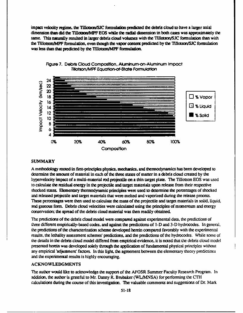
impact velocity regime, the Tilloson=C formulation predicted the debris cloud to have a larger axialdimension than did the MThlotsVWMPF EOS while the radial dimension in both cases was approximately thesame. This naturully resulted in larger debris cloud volumes with the T"llotson/SJC formulation than withthe Tilloun/MW formulation, even though the vapor conten predicted by the TlllotsonSJC formulationwas less than that predicted by the TiloonRMPF formulation.
Figure 7. Debris Cloud ComposItIon. Aluminum-on-Aluminum Impactlhlotson/MPF Equation-of-State Formulation
24~22
S,2
S18 % Vapor.16M
u 14 % Uquid142I121 U, %solid1- 0
E 6
4
0% 20% 40% 60% 80% 100%
Composdion
SUMMARY
A methodology rooted in first-principles physics, mechanics, and thermodynamics has been developed todetermine the amount of material in each of the three states of matter in a debris cloud created by thehypervelocity impact of a multi-material rod projectile on a thin target plate. The Tillotson EOS was usedto calculate the residual energy in the projectile and target materials upon release from their respectiveshocked states. Elementary thermodynamic principles were used to determine the percentages of shockedand released projectile and target materials that were melted and vaporized during the release process.These percentages were then used to calculate the mass of the projectile and target materials in solid, liquid,and gaseous form. Debris cloud velocities were calculated using the principles of momentum and energyconservation; the spread of the debris cloud material was then readily obtained.
The predictions of the debris cloud model were compared against experimental data, the predictions ofthree different empirically-based codes, and against the predictions of I-D and 3-D hydrocodes. In general,the predictions of the characterization scheme developed herein compared favorably with the experimentalresults, the lethality assessment schemes' predictions, and the predictions of the hydrocodes. While some ofthe details in the debris cloud model differed from empirical evidence, it is noted that the debris cloud modelpresented herein was developed solely through the application of fundamental physical principles withoutany empirical 'adjustment' factors. In this light, the agreement between the elementary theory predictionsand the experimental results is highly encouraging.
ACKNOWLEDGMENTS
The author would like to acknowledge the support of the AFOSR Summer Faculty Research Program. Inaddition, the author is grateful to Mr. Danny R. Brubaker (WL/MNSA) for performing the CTHcalculations during the course of this investigation. The valuable comments and suggestions of Dr. Mark
51-18

Hoffman of SAlCIShalimar are also noted with gratitude. Finaily, thanks go to Masrs. David Jerome and
Ronald Hum (WLAMNSA) for their guidance and assisance.
REFERENCES
1. Yatteau, J.D, Zemnow, R.H., and RechL, R.F., 1fiak Plate Perforation hdgellNSWC-TR-91-399, Dahlgren, Viria, 1991.
2. Bjorkman. M.D, Geiger, J.D., and Wilhelm, E.E., Sace_ Staion 1ntegrmaed Wall Design and Penetrationg Boeing Aerospace Corporation, Final Report, Contract NAS8-36246, Seattle,
Washington, 1987.
3. Greer, R. and Hatz, M., KAPPII User's Manual. Version . I Kaman Sciences Corporation, K92-17U(R), Colorado Springs, Colorado, 1992.
4. Tnoison, J.H., Mczli E=aoS for H3M itx Impal. General Dynamics, General AtomicDivision, Report No. GA-3216, 1962.
5. Allen, R.T., Eq~daiMn of State of Rocks and Minerals General Dynamics, General Atomic Division,Report No. GAMD-7834A, 1967.
6. Holian, K., and Burkett, M.W., "Sensitivity of Hypervelocity Impact Simulations to Eqns-of- State". Int.J. Impact Engng., Vol. 5, pp. 331-341, 1987.
7. Schonberg, W.P., Toward a Characterization of the Debris Cloud Created in a Hvervelocity Impact ona.Thi.nPlat, WL-TR-93-7028, Eglin AFB, Florida, 1993.
8. Rice, M.H., McQueen, R.G., and Walsh, J.M, "Compression of Solids by Strong Shock Waves", SoidStA w g VoL., Seitz, F. and Tumbull, D., eds., Academic Press, New York, 1958.
9. Rinehart, J.S., Stres Transiets in Soids, HyperDynamics, Santa Fe, New Mexico, 1975.10. Goldsmith, W., Im=ac The Theor and Physical Behaviour of Meldi•Soi., Edward Arnl|d,
London. 1960.
11. Zukas, J.A., eLal., llih Velocity Imp= Dynami. John Wiley, New York, 1990.
12. Maiden, C.J., Gehring, J.W., and McMillan, A.R.. l of F Mechanism oflamag IQ Thin IM8t by H3=,lociiy i&jmdes, General Motors Defense Research Laboratory, TR-63-225, Santa Barbara, California, 1963.
13. Anderson, C.E., Trucano, T.G., and Mullin, S.A., "Debris Cloud Dynamics", In. J. Impact Engng.,Vol. 9, pp. 89-113, 1990.
14. Piekutowski, AJ., "A Simple Dynamic Model for the Formation of Debris Clouds", It. J. ImpactEngng., Vol. 10, pp. 453-471, 1990.
15. Bell, R.L., et.al, CTH User's Manual Version 1.026, Sandia National Laboratories, Albuquerque, NewMexico, 1986.
16. Wilbeck, J.S., Scott, P.G., and Lew, T.M., Enhanced Fragment Letbaiy, AFATL-TR-88-105, EglinAir Force Base, Florida, August, 1988.
51-19
NEW DISCRETIZATION METHODS AND ITS APPLICATIONS IN MISSILEAUTOPILOT CONTROL
Kemin ZhouAssistant Professor
Department of Electrical and Computer EngineeringLouisiana State UniversityBaton Rouge, LA 70803
Final Report for:AFOSR Summer Faculty Research ProgramWright Laboratory/Armament Directorate
Eglin Air Force Base, FL 32542
Sponsored by:Air Force Office of Scientific Research
Boiling Air Force Base, Washington, D.C.
August 1993
52-1

NEW DISCR.ETIZATION METHODS AND ITS APPLICATIONSIN MISSILE AUTOPILOT CONTROL
Kemin ZhouAssistant Proiessor
Department of Electrical and Computer EnaneeringLouisiana State UniversityBaton Rouge, LA 70803
Abstract
This paper considers the sampled-data controller design using diu•tzsaioa method. Thework described here is motivated from the fact that the conventional textbook discretisationmethods do not take into consideration of the effects of the antiiasing filtars and the holddevices on the system performance, which may lead to severe performance deterioration whenthe sampling is not very fast. In this paper, we propose several simple alternative discretizationmethods which compensates the performance deterioration. Our methods are inspired by the
fact that the sampled-data controller (including the antialiasang tilters and the hold devices) canbe bounded by a conic sector with a linear time invariant optimal center. The fundamental ideaof our methods is to discretize the continuous controller in such a way that the frequency responseof the optimal center for the sampled-data controller approximate the frequency response of thecontinuous controller. This paper considers only some theoretical development of the proposedmethods. The applications of these methods in the misie autopilot control will be reported inthe subsequent research.
52-2

NEW DISCRETIZATION METHODS AND ITS APPLICATIONS IN MISSILE
AUTOPILOT CONTROL
Kemin Zhou
1 Introduction
It has been the common practice in modern control engineering that the controllers are implemented
using digital devices. This has been made possible because of the low cost and high fidelity of
modern digital devices and microprocessors. The digital implementation of a controller has also
the advantage that the changing of the controller design is made easy and cheap. Hence modern
control design process typically involves a step of implementing a controller using digital devices.
There are basically two ways to design a controller for this purpose: (a) design a discrete time
controller directly; (b) design a continuous controller first and then find a discrete time controller
by discretization. The first approach has been traditionally done by first discretizing the plant and
then design a discrete time controller for the discretized plant. This method ignores the intersample
behavior and, therefore, the performance of the sampled-data system is not guaranteed even if the
system behaves well on the sampling instants. Recently, much research has been done on the
direct sampled-data controller design, i.e., the discrete controller is designed so that the system's
continuous time performance criteria are satisfied (not just on the sampling instants), see (4] and
references therein.
This paper considers the more traditional approach (b), which is still widely used in practical
engineering design. We shall consider a dynamical system described by a general linear fractional
framework in Figure 1 with the generalized plant P which is partitioned accordingly as
P11 P12
1=[;21 P22]
Without loss of generality, we shall assume that the system performance objectives are to design
an internally stabilizing controller K(s) so that the transfer matrix from w to z satisfies certain
52-3
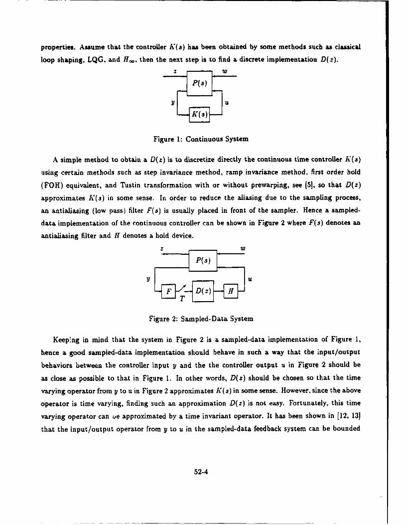
properties. Assume that the controller K(s) has been obtained by some methods such as classical
loop shaping, LQG, and H,,, then the next step is to find a discrete implementation D(z).
P(s)
K(,s)
Figure 1: Continuous System
A simple method to obtain a D(z) is to discretize directly the continuous time controller K(s)
using certain methods such as step invariance method, ramp invariance method, first order hold
(FOH) equivalent, and Tustin transformation with or without prewarping, see (5], so that D(z)
approximates K(s) in some sense. In order to reduce the aliasing due to the sampling process,
an antialiasing (low pass) filter F(s) is usually placed in front of the sampler. Hence a sampled-
data implementation of the continuous controller can be shown in Figure 2 where F(s) denotes an
antialiasing filter and H denotes a hold device.
P(3)
Il U
Figure 2: Sampled-Data System
Keep*ing in mind that the system in Figure 2 is a sampled-data implementation of Figure 1,
hence a good sampled-data implementation should behave in such a way that the input/output
behaviors between the controller input y and the the controller output u in Figure 2 should be
as close as possible to that in Figure 1. In other words, D(z) should be chosen so that the time
varying operator from y to u in Figure 2 approximates K(s) in some sense. However, since the above
operator is time varying, finding such an approximation D(z) is not easy. Fortunately, this time
varying operator can ue approximated by a time invariant operator. It has been shown in [12, 13]
that the input/output operator from y to u in the sampled-data feedback system can be bounded
52-4

in a conic sector with the linear time invariant "optimal center"
C(s) = TH(s)D(eaT)F(s), (1)
i.e., the time varying operator can be approximated by C(s). Therefore, as pointed out in (141,
D(z) should be chosen so that C(s) approximates K(s) in some sense.
Since the discrete controller D(z) obtained from the most of the existing conventional dis-
cretization methods only approximates K(s) in some sense, for example, the error of the frequency
response
IIK~(iw) - D(e.jwT)lIis small over certain frequency range, the closed-loop system performance can be significantly
deteriorated due to the sampler, the hold device, and the antialiasing filter. The purpose of this
paper is to propose some alternative discretization methods to (partially) overcome this difficulty.
For simplicity, we shall assume that H(s) is a zero-order-hold (ZOH) in this paper. The problem
with higher order hold can also be treated similarly.
The paper is organized as follows. Section 2 presents several rational approximations to the
ZOH transfer function. These approximations can be used to redesign a continuous time con-
troller so that this continuous time controller takes the sampling/hold process into account in the
discretization. The proposed approximations are also compared with the try -itional Pad6 approxi-
mations. Section 3 considers another class of approximations to the ZOH where some delay factors
are allowed. The proposed approximations are then combined with FOH equivalent discretization
method to give better discretizations for continuous time controllers. In section 4, a convex pro-
gramming discretization method is proposed. This method can be used to guarantee the closed loop
performance of the sampled-data system. Some simple illustrative examples are given in Section 5.
2 Rational Approximation of H(s)
One way to partially overcome the difficulty due to the conventional discretization methods is to
treat the antialiasing filter and the hold device as part of the plant, and then design a continuous
time controller K(s) for the augmented plant as shown in Figure 3. Note that lIT in H comes
from the fact that the sampler has a gain of 11T. Then a discrete time controller D(z) is obtained
by applying the conventional discretization procedures on k(s). There are several drawbacks
associated with this method. First of all, the controller k(s) will critically depend upon the
52-5

Y U
Figure 3: Continuous Controller Redesign
sampling period, therefore, the whole design process has to be repeated if the sampling period T
is changed. Secondly, the design of k(s) is not easy since H(s) is usually an infinite dimensional
system. The second difficulty can be avoided if a finite dimensional approximation of H(s) is used.
For the simplicity of notation, we shall denote
HT(S) := 1TH(S) - -sT(2T Ts1- ('2)
Our objective in this section is to summarize some well known approximations to HT(s) and to
provide some new approximations. In additional to the applications in the above design process.
these approximations are also useful in the discretization methods to be presented in the next section
if the approximants are minimum phase. A simple way to find a finite dimensional approximation
to HT(s) is perhaps to use the Padi approximation. Let
bo + bl(sT) + .. + b,,,(sT)t mHp~de(S) :
ao + al(sT) + " + a,,(sT)n'
We shaU call Hpde(s) the (n, m)-th order Pad6 approximation of HT(S) if the coefficients of the
power series of Hp•de match the first m + n + I coefficients of the power series of HT(S). The results
for some low order Padi approximations are shown in Table 1.
To obtain a better approximation. we shall conduct a numerical "earch. To fix the idea, we
.&d1 consider the approximation in the form of
l+2ýa( ) + 2(_)2fir.) +f/T(S) =
We shall consider two cases: (a) fiT(s) is minimum phase; (b) ftT(s) is possibly nonminimum
phase. The parameters are chosen to minimize the following approximation error:
max HT(jw)- -iTUCý')I
52-6

(n, m) Padi Approximation
1(1,0)
1 - (sT)/6
, 71 1-(sT)/31
(2,0) 1 + (sT)/2 + (sT) 2/12
1(2, 1) 1 + (sT)/2 + (sT):/12
1 - (sT)/0 + (sT) 2/60
( 1 + 2(sT)/5 + (sT)2/20
Table 1: Padi Approximation of
for some w, < = <" Note that the approximation accuracy beyond the frequency a,/2 is
not important since all signals beyond that frequency must be sufficiently attenuated for a good
controller design by the sampling theorem. The numerical experience shows that choosing W, =
will result in approximants with large approximation error at low frequencies. Therefore, W, = O.Si
will be used in our minimizations. To find a minimum phase approximation, we fix ý > 0 and
minimizing over a, /31, and /32. The minimization shows that the optimal parameters and the
approximation error change very little with different choices of the damping ratio ý. A typical set
of values are
S= 1, a = 0.001, ,31 = 1.0013:t 1, /32 = 0.3668
and the corresponding approximation error is
max jIIT(jw) - I-T(j•i = 0.0085.
With the above parameters, an approximation is given by
fIT(S)= -(+ a)1 1 (3)
It is interesting to note that this approximation is almost the same as the (2,0)-th order Pad6
approximation. In fact, the following transfer function is a good approximation of Hr(s) for any
2.75 - 3:1+ 2(s 2.
52-7

[f the approximation is allowed to be nonminimum phase. a second order best approximation is
found to be-0.1793 (i)+ 0.0687 ()
2"
II,~~(r =0.8172(~ + 0.2231 Z)
The frequency response errors for typic."' Pad6 approximations and the best approximations
are shown in Figure 4 and Figur- It is clear from the plots that Hr, with y = 2.9 is a very
good minimum phase approxima, 'ri. Note that if the inverse of Hm.,, is desired to be proper or
strictly proper, which is the case it the next section, then the numerator of Hm,, may be replaced
by (I + ac)k for some appropriate integer k and some sufficiently small a, for example, a < 0.001.
The use of these approximants in the design of K(s) is standard and will not be pursued here
further.
ilI
0 U U IiI U
Figure 4: The magnitude approximation Figure .5: The phase approximation errors
errors fIHT(iw) - HT~jw)I: (2, 0) Pad6 Z (HT(jw) - AT(jw)): (2, 0) Padi (solid),
(solid), (2,2) Pad- (dashdot), mtn vith (2,2) Pad6 (dashdot), A with 7 = 2.9
-y = 2.9 (dashed), (dotted) (dashed), (dotted)
3 Discretization Using FQH with Phase Lead Compensation
Another way, which has the potential to overcome both of the difficulties in the last section, is
to find a D(z) directly so that C(s) = 1 H(s)D( e T )F(s) approximates K(s) in some sense. For
example, D(z) may be chosen to minimize the frequency response between C(s) and K(s) over the
52-8

frequency range [O,wi] for some WL a =
mi max ,IK(jw) - IfH(jw)D(eJ-T)F(jw)I[. (4)D(2),,e [0, Wi] TI
However, this optimization is highly nontrivial. This is because D(z) cannot be an arbitrary transfer
matrix. It must be proper and has the same number of unstable poles as K(s). We shall propose
several methods in the next section to solve this optimization. In this section, we propose a simple
method to approximately solve this problem. The idea is as follows:
o Let P(s) and Ht(s) be minimum phase (except for some time dilay factors such as e-l" for
IA < T) approximations of F(s) and +,H(s), respectively, so that there is no unstable pole/zero
cancellation in forming the product of
D,(s) := [k-'Kk-l
and, furthermore. the rational part of D,(s) is proper. Then the discrete time controller D(z)
is taken as the discretization of D,(s). An approximation for F(s) is relatively easy to find
since F(s) is usually a rational stable and minimum phase transfer function. The minimum
phase approximation H/i,,n(s) in the last section can also be used here for Hlr(s). We shall
now discuss some alternative approximations below where HT(s) is allowed to contain a delay
factor.
We shall again consider the case where H is a ZOH. In this case
HT(S) := 7H(s) 1 - e-T
We shall consider several approximations of HT(s). We first note thatZ's) - 2:
TsHTr(s)= Ts e- 2
andsin rw 2:,.,j
HT(jw) = T e -
Hence a simple approximation of HT(s) would be
Hdelav(s) =e 2
This approximation has the advantage of having the exactly same phase as HT(s). This approx-
imation should be considered along with the fact that the performance degradation of the digital
implementation in most cases is due to the phase lag of the hold devices and the antialiasing filters.
52-9
To get a better approximation, we shall also consider the approximation in the form of
Hedev0 + 1= 2 (?) + a,(,?),I ~~(r_,) + 12 (T)
for some f > 0, a >_ 0, 13 > 0, and j2 _> 0. It is important to note that the zeros of H/•j°,+(s),
which is part of the D,(.s) poles, will be discretized to obtain the discrete time controller poles of
D(z). This is why the damping ratio f has been restricted to be positive. For the same reason, it
is highly undesirable to have small damping ratio ý. We shall choose these parameters to minimize
the approximation error in frequency domain:min max IHT(jW) - Hkde•v+(jw)(
(,0-alA 'MC [0,Wi,
for some w, _ 2 = T. It is noted that the above optimization will result in • = 0. Table 2 and
Table 3 show the optimization results with the fixed damping ratio •.
a 31 0 max IHT(iw) - Hdejav+(jWj)1
0.1 0.3854 0.1051 0 0.0160
0.2 0.3841 0.2106 0 0.0291
0.3 0.3824 0.3138 0 0.0417
0.4 0.3795 0.4140 0 0.0530
0.5 0.3717 0.5130 0 0.0629
0.6 0.3744 0.6079 0 0.0717
0.7 0.3708 0.6997 0 0.0793
0.8 0.3679 0.7904 0 0.0859
0.9 0.3627 0.8740 0 0.0918
1.0 0.3845 1.0207 0 0.0989
Table 2:
Some typical frequency responses for the approximation errors are shown in Figure 6-11. With
the above approximations, D,(s) can be written in the form of
Do(s) = ef G(s)
for some proper G(s). Now D,(s) can be discretized to obtain D(:). Since D,(s) has a predication
factor ef, it is not straightforward how the existing discretization formulas can be used. In the
52-10

a 31 32 maxjHr(j~w) - d&+j)
0.1 0.3936 0.0957 0 0.0076
0.2 0.3928 0.1915 0 0.0142
0.3 0.3929 0.2873 0 0.0207
0.4 0.3902 0.3800 0 0.0269
0.5 0.3884 0.4721 0 0.0326
0.6 0.3872 0.5638 0 0.0378
0.7 0.3834 0.6505 0 0.0426
0.8 0.3827 0.7405 0 0.0469
0.9 0.3794 0.8246 0 0.0508
1.0 0.3763 0.9073 0 0.0543
Table 3:
4s
Lut
* U 13i U LS L
Figure 6: The magnitude approximation Figure 7: The phase approximation er-
errors HTUjW) - HTUW)I1: H~deIay (solid), rors L (HT(jw) - HIT(jw)): fHdL.v (solid),
(1, 0) Pad6 (dashdot), AI, with ý = 0. 1 (1, 0) Padi (dashdot), Hdl,,,pg. with ý = 0.1
and w1i = ji(dashed), H~dea.s.V with ý = 0.1 and w, = +(dashed), Ad,,.,+ with ý = 0.1
and w, = 0.8wr (dotted) and w, = 2f- (dotted)
52-11

S. .• i" . .......... . ......
lei
*uI I S a * U I S a ii a a
Figure 8: The magnitude approximation Figure 9: The phase approximation er-
errors IHT(jUJ) - HT(iw): Hdjiv (solid), rors /_ (HT(jw) - HT(jw)): Hdejap ksolid),
(1, 0) Pad6 (dashdot), Hd.lav+ with . = 0.5 (1, 0) Pad6 (dashdot), Ad.,.,+ with ý = 0.5
and w, = , (dashed), HdeiaV+ with ý = 0.5 and w, = + (dashed), Adjdv+ with ý = 0.5
and w, = 01 (dotted) and wl = . (dotted)
........................ ...... ~......
I a I t
.iI
Figure 10: The magnitude approximation Figure 11: The phase approximation er-
errors .H"(iW) -.. T(jW: "qd-.a (solid), rors L (HT(jw) - HT(jW)): kdiay (solid),
(1,0) Pad6 (dashdot), Ad,.. with ý = 1 (1,0) Pad. (dashdot), Ad,,,,,+ with ý = 1
and wPd (dashed), /Hdej. wth ý = 1 and (0 P 'd (dashed), Hde.iga+ with ý = I
and w, = - (dotted) and w, = - (dotted)
52-12

following, we shall describe a procedure for the discretization of a LTI system with predications
using a First Order Hold (FOH). Let G(s) be a finite dimensional LTI system with a state space
realization
G(s) ]
We want to find an equivalent discrete time system for D,(s) := efiG(s). A ZOH equivalent
discrete time system can be found using the method described in Franklin et al [5]. We shall
describe a method using FOH. This discretization can be illustrated by the following diagram:
----T f f--------------------Lz--------u t)-!-.-..... .'...•.;, U(t) G ~ ) y(t) :
T i .Y• t. .. T
Our objective is to find the discrete time state space realization for the system in the dashed
box. The problem can be solved either in state space or in Z-domain. Since the FOH has the
following transfer function:-eT)2Ts + 1
FOH(s) =(1-e )Ts 2
the transfer matrix for the dashed box is given by
Gd(z) = Z {G(s)e'2'FOH(s)}
T1 )2 1 Ts+ 1
Computing the above 3-transform is usually complicated. In the following, we shall present a state
space solution.
Lemma 1 Let G(s) = [ B . Then a discrete time state space realization for Gd(z) is givenC D
by
G-i)(½r, + r2) b,(2r, + r2) - r2 + (r, + r 2 )
2 2Gd(Z) -"0 0 [c -ID c(r, + r2) + 2D
where
T= eaT = e2A, r1 2 e A,•d77B, r 2 = - e
52-13

Moreover, #,, ri, and f 2 satisfy the following relation:
0 0 1 ]ep 0 0 7,I T}.
0 0 1 0 0 0
Due to space limitation, the proof is omitted. The formulas for the discretized model using higher
order hold can also be derived similarly although the derivation is much more involved. It is useful
to note that the poles of the discretized model has the form of zx det(zl - eAT) where r = order of
hold, for instance, r = 1 for FOH and r = 2 for second order hold.
4 Discretization Using Convex Optimization
The optimization problem (4) in the last section can be solved if D(z) can be parameterized as a
convex function of some parameters. It is easy to see that most discretization methods. such as
step invariance, ramp invariance, and FOH equivalent, will result in a controller with poles at eAT
and 0. This motivates us the following approximation method.
Let the desired q-input and p-output discrete time controller D(z) have the following form:
(Z ) =zr det(zI - eAT)
for some r > 0 and m < r + n where n is the dimension of A aid ,i E RP q for i - 0,1,....mare
free parameter matrices. Now Go, Cal...., and a,, are chosen so that
min max A'(jw,) - -Hj).e-)~wo. -' [0, J1] 1 Ti
Note that this optimization is a convex problem and can be solved easily using standard techniques.
The parameterization for D, can also take a state space form if desired, for example, D. may be
parameterized as
Dz) =Orxr0
where C, is any matrix so that the system is observable and r[' and J, are free parameters to be
chosen.
52-14

Robust Stability Criterion
We should point out that finding a D(z) which minimizes problem (4) may not be necessary in some
applications and may require very high order controllers, i.e., large m and r. if the approximation
error is required to be very small. In many cases, it is more sensible to find a lower D(z) to minimize
some weighted approximation error. For example, in order to make sure that the sampled-data
system is closed loop stable, we should choose D(z) such that a dosed loop robust stability criterion
is satisfied.
A reasonable robust stability criterion in this case is
e.b := maxU(1 + P22(s)K(s))-' P22(s) (K(s) - TH(s)D.,(eT)F(S)) H.,,Note that this criterion is not exactly the robust stability criterion for the sampled-data system
since Ce(s) = +H(s)D•(eJT)F(s) is only the center of the sampled-data controller. Hence we shall
choose the parameters ai so that
min max 1(1 + P22(s)K(s))-' P22(s) K(s) - TH(s)D,(eJT)F(s)) .
Closed Loop Transfer Functions
We can also formulate the problem so that the parameters in D,, are chosen to minimize the closed
loop performance degradation due to sampling. Let
C.(s) = TH(s)D.(esT)F(s)
and denote the closed loop transfer function for the continuous system
T(s) = PII + P12 K (I- P22 K)-' P21
and the approximate closed loop transfer function for the sampled-data system
Td(S) = P11 + P12 C. (I - P22C.)-! P2 1.
Then
T(s) - Td(s) = P 12(I - KP22)-(K - C.)(I - P22C,)-'P 21
and the performance degradation due to the sampled-data implementation of the continuous time
controller can be measured by
max IIT(jw) - Td(jw)II•
52-15

Thus Ca, should be chosen so that the above performance degradation criterion is minimized. Since
C. appears nonlinearly in T(s) - Td(s), we shall propose the following optimization procedure,
which results in a convex optimization problem in each s-ep:
1. Let • = K;
2. Find matrices a,,i - 0, 1,. . ., m so that
c-= min max jnP12(I - KP 22 )-'(K -Ca)(I- P22 ')-'IP21
3. Let • = C,,
4. Find matrices ai, i = 0,1 .... m so that
er=minmaxjjP12(I - IP 2 2 f-'(K - C.)(I - P22k)`P211
5. if le - Eol < 6 where 6 is the tolerance, then stop. Otherwise, let c. = e and go to step 3.
5 Examples
The first example is taken from the paper by Rattan and Yeh [101. This example has also been
considered in [11, 71. The system considered in these papers is a single loop feedback system with
a continuous time plant G(s) and a continuous time controller K(s):
10 0.416s + 1C(s)=-- K(s)=7(s3+1)' 0.139s + I'
The diagrams for the original continuous time system and for the sampled-data system are shown
in Figure 12 and Figure 13, respectively. The sampling period is chosen to be T = 0.15.
r(t) yt-0- K(s) G(s) yt
Figure 12: Single Loop Feedback System
The best controller obtained by Rattan in [11] is
D(z) = 3.436z - 2.191
z + 0.2390
52-16

rtD(z) ZOR G(s) YMt
Figure 13: Sampled-Data Implementation
Using the approximation Hd/.v = e-f* for the ZOH transfer function, a discrete controller is
obtained using Lemma I as
3.4319z 2 - 3.6546z + 0.8828z(z - 0.3399)
We have also obtained a first order discrete controller using the robust stability criterion through
the convex programming method proposed in the last section. The controller is given by2.259z - 1.8133
z - 0.3399
which has the approximation error e,.b = 0.3248. The approximation error between K and Cc
is shown in Figure 14. The step responses of the continuous time system and the sampled-data
systems are shown in Figure 15.
-------- - --
W . . .... ... ...............
le te ale to lie to a a M1 It 34 ' S
Figure 14: Approximation Error: Figure 15: Step Responses: Continuous
G~w (K(jw) - +H(iw)D(ejwT))I (solid), Rattan (dashdot), D,, (dashed),
delay (dotted)
The step responses show that the first order approximation is not good enough, our second
52-17

order approximation using the robust stability criterion gives
D(--) =2.8474z2 - 3.0456z- + 0.7489z(z - 0.3399)
which has the approximation error (,.b = 0.1793. The approximation error between K and C,
is shown in Figure 16. The step responses of the continuous time system and the sampled-data
systems are shown in Figure 17.
f i
Figure 16: Approximation Error: Figure 17: Step Responses: Continuous
÷G(j,•) (K()jw) - +H(jw)D( T)) (solid), Rattan (dashdot), D, (dashed)
The second example is taken from Katz [61 where it is shown that most of the conventional
discretization methods will result in controllers that cannot stabilize the sampled-data system.
The system considered is a double integrator with
863.3 2940s + 86436G(s) = , K(a)=s2 '(s +294)2
and T = 1/33. We again employ the convex programming discretization method in the last section
with the robust stability criterion. Then a second order approximation gives
_ 1.5464z 2 - 1.3793z + 0.3059(z - 0.0003)2
which has the approximation error c. = 0.6136. The step response of the continuous time system
and the sampled-data system are shown in Figure 19. The approximation error between K and Ca is
shown in Figure 18. The performance can be further improved using a higher order approximation.
52-18

Figure 18: Approximation Error: Figure 19: Step Responses: Continuous
(I- Iw("e) K(j- )- T+H(j)D(eJ T)I (solid), D,, (dashed)
6 Conclusions
In this research project, we have considered the sampled-data controller design using discretization
method. Several new and simple discretization methods have been propoGed. These new methods
can be used to compensate the performance deterioration due to the discrete implementation of a
continuous controller. The applications of these methods in the missile autopilot control will be
reported in the subsequent research.
Acknowledgment
The author would like to thank the support by many people in WL/MNAG of Eglin AFB, in
particular, the author is very grateful to Dr. James R. Cloutier and Dr. Chris D'Souza for their
support which made the research in the Lab. exciting and fruitful.
52-19

References
(11 B. D. 0. Anderson, "Bode Prize Lecture (Control design: moving from theory to practice),"
IEEE Control Systems, Vol. 13, No.4, pp. 16-25, August 1993.
[2] K. J. Astrom and B. J. Wittenmark, Computer Controlled Systems: Theory and Desig'n, 2nd
Ed., 1990, Prentice Hall, Englewood Cliffs, NJ. i
[3] S. Boyd and C. H. Barratt, Linear controller design: limits of performance, Prentice Hall,
1991.
[4] T. Chen and B. Francis. Sampled-Data Control Systems. Lecture Notes. January 1993.
[5] G. F. Franklin, J. D. ?owell, and M. L. Workman, Digital Control of Dynamic Systems, 2nd
Ed. 1990, Addison-Wesley Publishing Company, Inc.
[6] P. Katz, Digital Control Using Microprocessors, Englewood Cliffs, NJ: Prentice-Hall, 1981.
[7J J. P. Keller and B. D. 0. Anderson, "A new approach to the discretization of contini'ous time
controllers," IEEE Trans. Automat. Contr., Vol 37, No. 2., pp. 214-223, February 1992.
[8] R. A. Kennedy and R. J. Evans, "Digital redesign of a continuous controller based on closed
loop performance," Proc. 29 IEEE Conf. Dec. Contr., HI, 1990, pp. 1898-1901.
[9] H. H. Niemann, "A frequency domain design method of sampled-data compensators," F 'oc.
American Contr. Conf., San Diego, CA, May 1990, pp.1156-1158.
[10] K. S. Rattan and H. H. Yeh, "Discretizing continuous data control systems," Computer-Aided
Design, Vol. 10, pp. 299-306, 1978.
[11] K. S. Rattan, -Digitalization of existing continuous control systems,"IEEE Trans. Automat.
Contr., Vol. AC-29, pp. 282-285, 1984.
[12] P. M. Thompson, G. Stein, and M. Athans, "Conic sectors for sampled-data feedback system,"
Systems and Control Letters. Vol. 3, pp.77-81, 1983.
(131 P. M. Thompson, R. L. Dailey, and J. C. Doyle, "N'w conic sectors for sampled-data feedback
system," Systems and Control Letters, Vol. 7. pp.39 5 --404, 1986.
[141 P. M. Thompson, R. Pena, and Y. Wong, "Design of sampled-data compensators based on the
use of conic sectors," Proc. American Control Conference, pp.1462-1464, 1986.
52-20
22-KHZ VOCALIZATIONS AND STRESS IN RATS
Suzanne C. Baker
Assistant Professor
Department of Psychology
James Madison University
Harrisonburg, VA 22807
Final Report for:
Summer Research Program
Armstrong Laboratory
Sponsored by:
Air Force Office of Scientific Research
Bolling Air Force Base, Washington, DC
August 1993
53-1
22-KHZ VOCALIZATIONS AND STRESS IN RATS
Suzanne C. BakerAssistant Professor
Department of PsychologyJames Madison University
Abstract
Rats sometimes emit 22 kHz ultrasonic vocalizations in response to
stressful stimuli. We examined the contexts in which this vocalization occurs
as well as the physical characteristics of this vocalization in order to
investigate the usefulness of 22 kHz calls in the evaluation of AF-relevant
stressors. We digitally recorded and analyzed rat ultrasonic vocalizations in
several contexts. In our investigations, rats vocalized in response to
acoustic startle stimuli, in response to light touch by humans, and when
isolated and undisturbed for long periods. The basic structure of the
vocalizations appears to be similar in all these situations, although the rate
of vocalizing varies widely across these situations. High-fidelity recordings
were made of rat ultrasonic vocalizations in the acoustic startle testing
paradigm in order to perform detailed analyses of the physical characteristics
of these signals (e.g., intensity, frequency modulation, onsets and offsets),and to evaluate the relationship between these acoustic parameters and
characteristics (such as intensity) of stress-inducing stimuli.
53-2

22-KHZ VOCALIZATIONS AND STRESS IN RATS
Suzanne C. Baker
IntroductionThe work of the Performance Extrapolation Branch, Radiofrequency
Radiation Division, Armstrong Laboratory, is directed at developing,
validating, and applying animal models for predicting the effects of Air Force
relevant stressors such as electromagnetic radiation and chemical and
toxicological agents. Rodent and nonhuman primate models are focLsed on. Inparticular, rats have proved to be useful as subjects in a variety of previousstudies in this laboratory, particularly in examining effects ofelectromagnetic radiation and organophosphate exposure (e.g, Murphy et al,1990, 1991; Miller et al, 1992, 1993). A reliable, convenient, and efficientmethod of assessing psychological states in rodents (such as stress,
emotionality, or anxiety) would therefore be of great value in this research
effort.Rats emit vocalizations in response to a variety of stimuli. While some
of these vocalizations are in the range of human hearing, most ratvocalizations are ultrasonic (i.e., around 20 kHz or above). Ultrasonic
vocalizations (UVs) in the range of approximately 40-70 kHz and higher occur
in agonistic and sexual situations (Sales, 1972a, 1972b; Thomas and Barfield,
1985). These are brief calls (approximately 3-65 msec) which sometimes showmarked frequency modulation. When given by the male during sexual behavior,
these calls seem to influence female proceptive behavior (Barfield and Thomas,1986). However, there is no conclusive evidence concerning the function of
these calls in agonistic situations (Takahashi et al, 1983).Vocalizations of around 19-24 kHz (the "22 kHz vocalization") have been
noted in the following situations (see Baker et al, 1991):-males prior to and following ejaculation (Barfield and Geyer, 1972; Brown,
1979)-males in agonistic situations (Sales, 1972)-exposure to a predator (Blanchard et al, 1991; 1992)
-physical restraint (Sewell, 1967; Brudzynski and Ociepa, 1992)-home cage, isolated from colony (Francis, 1977)
-light touch by humans (Brudzynski and Ociepa, 1992)
-shock (Tonoue et al, 1987; van der Poel et al, 1989)-avoidance learning (DeSalvia et al, 1990; Cuomo et al, 1992)-acoustic startle (Kaltwasser, 1990, 1991; Murphy et al, 1993)
53-3

"22 kHz" ultrasonic vocalizations are typically fairly long duration
(500-1200 msec) pulses of approximately 19-24 kHz with little frequency
modulation. Occasional pulses are longer than 2 sec. The beginning or end of
a pulse may show a brief, rapid rises or falls in frequency. Pulses are
frequently emitted in bouts or series of 3 to 20 pulses or more, with pausesbetween the pulses. The first pulse of a bout is often of longer duration
than the following pulses.
Many of the contexts in which the 22 kHz call occurs clearly might be
stressful or anxiety-provoking to the rat. However, the communicative
function of the call, if any, has not conclusively been demonstrated. The
function of the 22 kHz call in sexual behavior is not known (Barfield and
Thomas, 1986). It has been suggested that emission of the 22 kHz call by
submissive rats in agonistic situations inhibits aggression by dominants;
however, experiments using deafened and muted rats have not provided clear
support for this hypothesis (Thomas et al, 1983; Takeuchi and Kawashima,
1986). Blanchard et al (1991) suggests that these calls might function as
alarm calls in the colony situation. Administration of anxiolytic drugs such
as benzodiazepines decreases 22 kHz UVs following shock (Cuomo et al, 1988;
Miczek et al, 1991), strongly suggesting that in at least some contexts thesevocalizations are associated with stress or anxiety states. Numerous recent
studies have confirmed the usefulness of rat UV measures in behavioral
teratology and in the study of pharmacologic effects (e.g., Insel & Winslow,
1991; Miczek et al, 1991; Elsner et al, 1990; Cuomo et al, 1990; Elsner et al,
1988; Bignami et al, 1992).The use of vocalizations as an indicator of the internal state of the
animal has some distinct advantages over some other methods:
(1) Vocalization is a naturally-emitted response which has ethologicalvalidity; it occurs in response to naturally-occurring stressors.
(2) Because vocalization is a response which is part of the rat's normalbehavioral repertoire, subjects do not have to be trained in any way to emit
the response. This is in contrast to escape, avoidance, or discriminationresponses which require training. Vocalization can be thought of as a
naturally-occurring "self-report" measure of the animal's emotional state.(3) Measurement of vocalizations is a non-invasive procedure, unlike, for
example, the collection of blood for analysis. Therefore the measuring
technique itself does not impose further stress on the animal and does not
require sacrificing the animal. In addition, vocalization can be measured
repeatedly in the same animal without adverse effects on the subject.(3) Measurement of vocalizations can be performed in many experimental
situations often without extensive modification of the study protocol or
apparatus.
53-4

Rat vocalizations and startle
The acoustic startle response has been extensively used in studies ofpharmacologic and toxic effects. In this lab, startle responses have been
studied to assess the effects of organophosphate toxicity (e.g., Miller et al,1992). UVs are emitted by rats in the acoustic startle testing situation(Kaltwasser, 1990, 1991; Miczek & Vivian, 1993; Murphy et al 1993) . The
pattern of calling is influenced by the startle stimulus. A startle stimulusoccurring during a bout of pulses typically causes a brief interruption ofcalling, followed by the beginning of a new bout.
Parameters of the startle response and UVs are sometimes correlated.For example, rats on diazepam withdrawal exhibit higher-amplitude startle
responses and as well as a higher rate of UVs than controls (Miczek and
Vivian, 1993). In other cases, parameters of UV and startle are not
correlated (Murphy et al, 1993), suggesting that these two measures may
reflect somewhat different underlying states.
During the summer research period, efforts were directed at the
following tasks:-Review of the current literature on adult rat UVs, rat pup UVs, and UVs of
other rodent species. The focus was on the usefulness of vocalization
measures as indicators of stress, anxiety, or emotionality.-Broader examination of the contexts in which vocalizations are emitted by
rats, in order to assess their usefulness in the measurement of stress and
other emotional states.-More detailed examination of spectral (frequency) characteristics of thevocalizations. Some earlier reports have mentioned the possibility of
harmonic components of the 22 kHz call, but this possibility hasn't been
closely investigated.-Validation of measurement and recording techniques used in the lab, inparticular, comparison of high-fidelity recordings with recordings made using
bat detectors.
General Method
Subjects
The subject pool consisted of 24 adult male Sprague-Dawley rats. Ratswere obtained from Charles River and were 43 days of age when they arrived at
Brooks AFB. The rats had been subjects in other studies prior to those
described here. Most had been food deprived for approximately one year, but
had been on ad lib feed for several months prior to the time they were testedhere. In addition, most subjects had been repeatedly handled in a Functional
Observational Battery. Most of the subjects also had participated in a
53-5

previous study of acoustic startle-induced vocalization (Murphy et al, 1993),
during which they had been tested in the startle apparatus 2-3 times. All
rats were 19-20 months old at the time of the investigations reported here.Rats were housed in standard cages and had continuous access to fc-d andwater, except when being tested. Rats were maintained on a 12-hr 'D
schedule, with lights on at 0600 and off at 1800.
ApparatusAll testing equipment (except when rats were tested in their home cages)
was located inside a sound-attenuated chamber. A San Diego Instruments Model
SIC startle apparatus was used to present the acoustic startle stimuli. Thebasic design of the apparatus was a plexiglass tube mounted on a platform
which detected characteristics of the startle response. The platform and tube
were enclosed inside a chamber. Rats weighing over 600 g were tested in 11.3
cm diameter tubes; smaller rats were tested in 8.3 cm tubes. Acoustic startle
stimuli were 108 dB broadband signals, 40 msec in duration. Presentation of
the startle was controlled and startle responses were recorded using a SanDiego Instruments SR-Lab Control system.
Vocalizations were detected and recorded using ultrasound detectors
("bat detectors;" Ultrasound Advice Model S-25) and/or a high-fidelity
recording system consisting of a microphone (Bruel & Kjaer Type 4135) with
attached cathode follower (B & K Type 2633) and amplifier (B & K Type 2610).
Sensitivity of the bat detector microphone capsule is reported as better than
-57 dB +/-3 dB from 20 to 120 kHz and better than -70 dB at 180 kHz (ref 1V/microbar). The bat detector could be used in either of two settings. The
"frequency divide" setting could be used to detect signals across the entire
range of sensitivity of the instrument. In the "heterodyne" setting, the bat
detector could be tuned to detect signals in a relatively narrow band +/- 5
kHz on either side of a selected frequency.
Frequency response of the B & K system (with microphone shield removed
as for recording) extended to 200 kHz, approximately flat +/-l dB to 100 kHz.The B & K system was calibrated relative to 20 microPa sound pressure using a
pistonphone calibrator (B & K Type 4228) coupled to the B & K microphone. Thecalibrate signal produced by the pistonphone was 250 Hz at 123.98 dB above the
reference sound pressure. Ambient pressure and corresponding correctionfactors were determined using a B & K UZOO04 barometer.
Output from the vocalization detection systems was monitored, digitized,and stored using Global Lab data acquisition software (ver. 2.20) and a Data
Translation A/D board (#2831-G). For some studies, a custom-written computer
program (M.R. Murphy, unpublished) was used to detect UVs in the data files
following collection of the data. This program was designed to identify all
signals above a specified amplitude which exceeded a specified duration.
53-6
I. 6-Hour Vocalization RecordingsIt has been reported that rats emit unelicited, "spontaneous" UVs (both
22 kHz and higher frequency) when in their home cages and isolated from therest of the colony for long periods (Francis, 1977; Lewis and Schriefer,
1982). We examined the occurrence of UVs in a similar testing situation inorder to compare vocalizations in this context with those occurring in the
startle paradigm.Subjects. Seven rats from the subject pool were used. Subjects which
had shown high levels of vocalization in earlier startle tests (Murphy et al,1993) were selected, since rates of vocalizations are typically low in thiscontext and the goal was to examine the general pattern of UVs in this context
for comparison with UVs emitted during startle testing.Apparatus. Subjects were tested in 24 x 45 x 20.5cm cages with wire
lids. Cage bottoms were covered with shavings, and food and water wereavailable ad lib during testing. The testing cage was placed inside a
chamber, which was kept open to allow it to be illuminated. The testing cageand outer chamber were located inside the sound-attenuated chamber.Vocalizations were detected using a bat detector and were recorded usingGlobal Lab. The bat detector microphone was suspended approximately 6cm abovethe cage lid. The bat detector itself was located outside the chamber, withthe volume setting turned all the way down so that signals were not audible.Light was provided by a desk lamp with a 75w bulb, located so that the ratcage was illuminated. A timer was used to control the light so that it was
consistent with the rat's normal L/D schedule.Procedure. Subjects were tested individually. Each subject was removed
from its home cage and placed in the testing cage and chamber. Subjects weregiven at least 20 min to habituate to the testing cage and chamber. The batdetector's frequency divide setting was used, so that any detectable signalwithin the bat detector's frequency range would be picked up. Each test
lasted 6 h. Data were collected using a sampling rate of 1000 Hz, which hadbeen shown to be suitable in previous tests using startle (Murphy et al,1993). Some data collection periods occurred during the animals' light phase(LP) and some overlapped the light and dark phases (LDP). The amount of timein the testing session prior to the beginning of the dark phase ranged from
70-135 min, with the lights going out, on average, 107 min into testing. Dueto technical difficulties, one testing session took place completely in thedark (the session began 115 min prior to the normal beginning of the darkphase for this rat). Of the 7 rats tested, 3 were tested during both timeperiods; the remainder were tested during only the LDP.
Results and Discussion. At least some signals were detected during eachdata collection session using the vocalization detection program. However,only in two cases did these signals clearly show characteristics typical of
53-7

the 22 kHz vocalization, such as bout structure. It is possible that many of
these detected "signals" were not vocalizations but were due to rat movements.
Scratching the cage walls and causing the metal parts of the cage to contactone another are known to cause detectable high frequency sounds.
No signals which could unequivocally be identified as vocalizations were
detected during any of the 3 1 :ht phase data collection periods. Clearvocalizations were detected during 2 of the 7 (28.6%) dark phase periods. In
one of these cases, a clear period of UVs began 163.85 min into the testing
period, approximately 49 min into the dark phase. This bout of vocalizations
continued for 10.48 min. No further UVs were detected during the session. In
the other session where UVs were detected, the rat began vocalizing
approximately 20 min into the habituation period, while the calls were being
monitored auditorially prior to data collection. Data collection was begun,
and the rat continued vocalizing for 7 min into the session. UVs began again
at 271.5 min into the session, approximately 148 min into the dark phase. The
bout of calling lasted approximately 3.5 min.Francis (1977) reports calling by isolated rats during both the dark and
light phases, with a peak in calling approximately in the middle of the darkphase. It should be noted that the amount of time the animals spent
vocalizing in Francis' study was extremely small, and several animals showed
peaks in calling during the light phase also. Small sample sizes in both
Francis' study and this one make comparisons difficult.
The bout structure of the calls which were detected here appears to besimilar to that of calling bouts observed during startle testing. UVs were
given in series of several pulses, with longer pauses in between the series.
Pulse duration was roughly the same as seen in startle tests. Although in
some cases, the intensity of these spontaneous calls was as high as thoseobserved during startle testing, in other cases the intensity was much lower.
Vocalization bouts generally began with series of lower intensity pulses,
working up to higher intensity and then decreasing again so that the final few
series in a calling bout consisted of quite low intensity pulses.
II. Vocalization in Response to Touch
Brudzynski and Ociepa (1992) report that rats vocalize in response to
gentle touch. Subjects were tested using a technique similar to that used by
Brudzynski and Ociepa in order to compare parameters of UVs in this contextwith those given in the acoustic startle paradigm, and in order to examine
more closely the spectral characteristics of the calls.
Subjects and Apparatus. Nineteen subjects were selected at random from
the subject pool. Subjects were tested in their home cages, in the colony
room. Vocalizations were detected using a bat detector.Procedure. Subjects were tested during the light phase. The subject's
53-8

cage was pulled away from the cage rack, and the bat detector was held near
the open end of the cage. The distance of the microphone from the rat during
testing was highly variable, depending on the rat's movements, but ranged from
approximately 4-30cm.The experimenter then began touching the rat gently with a gloved hand.
Rats were touched briefly (approximately .5 sec/touch) two or three times,approximately every 20-30 sec. Touches were directed to the dorsal neck and
spine area, since Brudzynski and Ociepa had found touches in this region to bemost likely to elicit UVs from their subjects. Latency to the first UV was
noted. Until the rat began vocalizing, the frequency divide setting on the
bat detector was used. Once the subject began vocalizing reliably, the batdetector was changed to the heterodyne setting, and the frequency selectiondial was slowly moved through its settings. Frequencies at which calls weredetected were noted. This was done up to 3 times, or until the rat stoppedvocalizing. Calls were monitored on headphones throughout testing. Testingwas discontinued after 15 min if the rat had not begun vocalizing at that
point. No more than 4 animals were tested per day, in order to minimizedisturbances in the colony room which might have influenced the animals.
Results and Discussion. Thirteen of the 19 subjects (68.4%) vocalized inresponse to repeated touch. This percentage is very close to that obtained byBrudzynski and Ociepa (66.7%). The average latency to vocalize for 11 of the12 subjects which vocalized was 331.17s. Latency was not recorded for one
subject.When vocalizing, rats usually remained still, crouched down on all
fours, with their heads down. One rat vocalized while rearing, exploring thecage, and grooming its face. In many cases, the rat's sides and nose could beseen to move when the calls were emitted. In a more general sense, the calls
did not seem to be associated with submission or fear, since some rats which
spent the entire 15-min session crouched in a corner (apparently submissive)did not vocalize at all, and some rats which did vocalize spent a great dealof time exploring the cage and investigating the area near the experimenter
and the microphone.
As Brudzynski and Ociepa noted in their study, UVs did not seem to be indirect response to touch, as they rarely if ever occurred immediatelyfollowing touches. There was generally an interval of several seconds between
touches and UVs.
With one exception, calls detected were clearly given by the animalbeing tested, and no calls were detected from other colony animals. This wasdetermined by periodically pointing the bat detector away from the animalbeing tested and toward other animals. In one case, UVs were detected duringa test, but they were extremely faint. The subject in this case also did not
show other signs of vocalization (e.g., rhythmic movement of the sides). The
53-9
calls appeared to be emitted by another nearby rat, since they increased in
intensity when the bat detector was pointed towards this animal. This could
not be determined with certainty since the animal did not vocalize for a longenough pericd.
The calls showed the typical bout structure reported for 22 kHz calls;
they were emitted in series consisting of several pulses. In all cases where
it the animals vocalized long enough to examine it, frequencies above the 19-
24 kHz range were detected. Typically, the output generated by the bat
detector sounded most intense at around 19-24 kHz; however, for individualrats, frequencies of approximately 38, 45, 50-60, and 70 kHz were commonly
detected. Tuning the bat detector to frequencies falling between these would
result in no signal being detected. In most cases, the signals detected were
clear and intense. In some cases, the bat detector would produce faintsignals signifying sound above 100 kHz. The exact frequencies which were
detected varied among rats, and sometimes varied slightly within the same rat.It is not known if these higher (>25 kHz) detected frequencies were
actually part of the call and were produced by the rat, or were due to some
aspect of the bat detector's functioning. The higher-frequency signals showedthe same pulse/series structure typically seen with the 22 kHz call, and the
signals were correlated with behavioral signs of vocalization emission. The
signals were not detected by the bat detector when it was not directed towarda vocalizing rat, so the signals were not simply part of the ambient noise
environment.
III. Multiple-Channel RecordingsPrior tests of UVs during startle (Murphy et al, 1993) utilized the bat
detectors in the frequency divide mode. In this mode, the bat detectorresponds to any signals which are present across its entire sensitivity range.
This type of recording therefore does not provide information concerning the
frequency of these calls. In order to further investigate the spectral
characteristics of acoustic startle-induced UVs, vocalizations were recorded
during startle tests using several bat detectors, each tuned to detect signals
in a different frequency range.
Subjects and Apparatus. Two rats from the .3ubject pool were used inthis test. They were selected because of their propensity to vocalize in the
startle paradigm. Acoustic startle stimuli were presented and startleresponses were measured using the San Diego Instruments startle apparatus and
control system. Vocalizations were detected using several bat detectors, eachof which was tuned to a different frequency using the heterodyne circuit. For
the "4 mic" tests, 4 bat detectors were used, one tuned to each of thefollowing frequencies: 24 kHz, 40 kHz, 70 kHz, and frequency divide. For the
"6 mic" tests, 6 bat detectors (tuned to 22 kHz, 40 kHz, 50 kHz, 60 kHz, 70
53-10

kHz, and frequency divide setting) were used. :n both tests, the bat detector
microphones were located inside the startle chamber, while the bat detectors
themselves were located outside the chamber. The microphones were attached in
an array near openings at one end of the plexiglass startle tube. The
distance from the microphones to the tube was approximately 1.5cm; the
distance from the microphone to the rat varied between approximately 3 and
8cm, depending on the rat's movements. Global Lab data acquisition software
was used to display the output of all channels and to record the data.
Procedure. One subject was tested twice, once using the "4 mic"
procedure and once using the "6 mic" procedure. The other subject was tested
using only the "6 mic" procedure. A sampling frequency of 1000 Hz was used
for recording. Both rats were tested during light phase. The startle testing
procedure used was identical to that used by Murphy et al (1993). Rats were
tested individually. Each subject was brought into the sound-attenuated
chamber and then placed in the startle apparatus. The startle chamber doors
were closed, and a five minute habituation period began. Following the 5-min
habituation period, 20 acoustic startle stimuli were presented at 1 minute
intervals. Following the last startle, the subject spent a final 5-min period
in the apparatus before being removed and placed back in its home cage.
Characteristics of the startle (vmax, tmax, etc) were displayed on the
monitor, but these data were not utilized in this study.
Results and Discussion. Both subjects vocalized readily in the startle
paradigm. Signals were detected on all frequency settings, although there
were clear differences at the different settings. In general, when they
appeared, signals at each setting showed the same pattern - several pulses in
series, with these series of pulses separated by longer pauses. Quite often,
signals recorded on different frequency channels would begin and end
simultaneously, suggesting that these were part of the same vocalization
pulse. However, the intensity of the signals recorded at the different
frequencies varied greatly. The 22-24 kHz signals were the strongest, and
they remained fairly strong throughout the 30 min testing session. Other
signals were generally of lower intensity, often dropping off or completely
ceasing before the end of the session. The 60 kHz channel often registered no
signal at all at the same time the others were indicating high intensity
signals.
These results cannot be interpreted unequivocally. The results are
consistent with those for the touch-elicited UVs discussed above. In both
cases, the bat detector registered the strongest response when tuned to
approximately 19-25 kHz, with other settings showing lower intensity responses
and some none at all. As was stated above, it is possible that these higher
frequency components are due to some aspect of the recording system and are
not produced by the signalling animal. The results suggest, however, that the
53-11

"22 kHz" call have a more complex frequency structure than has been reportedpreviously.
IV. Recordings in Startle Apparatus
We recorded each rat's vocalizations in the startle testing paradigm.
The goal was to use the B & K recording system to obtain high-fidelityrecordings of rat vocalizations in the testing situation.
Subjects and Apparatus. All 24 subjects from the subject pool wereused. Acoustic startle stimuli were presented and startle responses were
measured using the San Diego Instruments startle apparatus and control system.Vocalizations were recorded using the B & K recording system and the Global
Lab data acquisition system. A bat detector was also used to monitorvocalizations.
The B & K microphone and cathode follower were suspended approximately
3.2cm above several openings in the plexiglass startle tube, at the end of the
apparatus nearest the rat's head. Output from the microphone was then sent to
the amplifier, and from there to the Data Translation A/D board. The
converted signal was then displayed on a monitor using Global Lab.The bat detector microphone was suspended approximately 2.4cm above a
hole in the center of the startle tube. Extensive experience with the bat
detector had demonstrated that it was sensitive enough to pick up
vocalizations when located at this point. The bat detector itself was located
outside the startle chamber.
Procedure. Prior to testing any rats, a 5-sec calibrate signal was
recorded (using the pistonphone calibrator) at a sampling rate of 50 kHz. The
correction factor for barometric pressure also noted. A new calibrate signalwas recorded after every four rats had been tested. The microphone shield was
removed during data collection.
All rats were tested during the light phase. The startle testingprocedure used was identical to that used by Murphy et al (1993) and described
above. Each rat was tested individually. Vocalizations were monitored during
the 5-min habituation period by listening to the audible output of the bat
detector on the "frequency divide" setting, and by visually monitoring theoutput of the B&K system using Global Lab. Volume on the bat detector was
turned down prior to recording so that the bat detector output was not audible
during this time.After the startle stimuli began and when the rat was vocalizing
reliably, 2 20-sec samples of vocalizations were recorded. We attempted to
record 2 samples from each rat, one from the first third of the startle
session and one from the final third, in order to examine whether the
parameters of the calls change across the startle session. The position of
the rat in the startle tube was noted prior to recording. We attempted to
53-12
record only when the rat's head was located at the same end of the tube as theB&K microphone. Once two samples had been recorded from the rat, it wasremoved from the startle apparatus and placed back in its home cage. Startletubes were cleaned as necessary between trials.
Results and Discussion. Recordings were obtained from 20 of the 24subjects (83%). Four of the subjects apparently did not vocalize at all
during the test. The percentage of animals vocalizing is higher than thatreported in other studies (Kaltwasser, 1990, 1991; Miczek and Vivian, 1993);
13A>chl : R83A% a-19.899%s( -0
9.e Tine (sac) L9.96 I
*B>RB3A 19.89968( 21953>
S.Tne (Sec)
Figure 1.
however, it should be noted that the subjects tested here had previously been
tested for vocalization in the startle paradigm and were selected from alarger group partly on the basis of their propensity to vocalize in thissituation.
Analyses of the results are not yet complete. Parameters to be examinedinclude duration of the pulses, spectral characteristics of the calls, and
intensity measurements (rise-decay times, maximum intensity). These analyses
should enable accurate characterization of the frequency of the calls, and adetailed assessment of the higher frequency (above 25 kHz) components of thecalls, if they exist.
Preliminary analyses utilizing waveforms, spectrograms, power spectra,and energy distributions of ultrasonic rat vocalizations indicate that the
53-13
calls obtained in this study are acoustically similar to those reported
previously by other investigators (Kaltwasser, 1990, 1991). Figure 1 shows a
series of intense, narrow-band pulses emitted in rapid succession by one
subject. Energy of the pulses in this series is centered around 22 kHz. An
expanded view of several of these pulses is shown in Figure 2. Frequency
[3A>chl: R83 4.23315( -29>
.6Tne (sea) 4.233
>R83A 4.23315< 21167>
Nz
O.AW Tine (sea) 4.233
Figure 2.
modulation tends to occur over a range of about 5 kHz. Intensity of most calls
exceeds 90 dB (re 20 uPa) sound pressure level. Call intensity, frequency
modulation, onset-offset transients, rate of emission, and number of pulses
per series will be examined to investigate the relationship between these
parameters and characteristics of stressors.
V. B & K Microphone/Bat Detector Comparative Recordings
Simultaneous recordings using the B & K recording system and the bat
detector were made in the startle paradigm. The goal was to obtain recordings
for the purpose of comparing parameters of recordings obtained using these two
different systems.Subjects and Apparatus. Because the goal was to determine the
comparability of recordings obtained using the B & K and bat detector
recording systems, subjects were chosen on the basis of their propensity to
53-14

vocalize in the startle situation. All subjects had been previously tested in
the startle paradigm. Rats were tested in the startle apparatus.Vocalizations were recorded using both the B&K system and the bat detector.
Data were collected from both systems using Global Lab. Microphones werelocated as in the startle tests (see above).
Procedure. All recordings were made during the rats' light phase. TheHF channel of the bat detector was used for recording. Data from both systemswas simultaneously collected and displayed using the Global Lab system.
Sampling rate was 125 kHz for both systems.The startle procedure was the same as that used during previous startle
tests (see above). A 5-min habituation period in the startle apparatus was
followed by startle stimuli at 1-min intervals. Vocalizations were monitoredvisually using Global Lab and auditorially using the bat detector during the
habituation period. When the rat began vocalizing, the gain setting on thebat detector was adjusted to make the amplitude of the signal from the batdetector approximately equivalent to the amplitude of the B & K signal.
Recordings were made after the startles began. Two 20-sec sample
recordings were made from each rat. Since the goal was to record as manyvocalizations as possible in order to obtain an adequate sample for comparison
purposes, we attempted to record during inter-startle intervals in which the
rat was vocalizing consistently and strongly. During recording, the volume
setting on the bat detector was turned down so that its output was notaudible. Prior to each recording, the location of the rat was checked to
ensure that the rat's head was at the end of the startle tube closest to themicrophone. Startle procedures were halted and the rat was removed from the
startle apparatus as soon as 2 recordings had been made.Results and Discussion. All rats vocalized during the procedure. Some
rats began vocalizing during the habituation period, but recordings were notmade until startle stimuli began. (One subject, for example, began vocalizing
12 sec into the habituation period.) Analyses of these data are not yetcomplete. Parameters similar to those listed above (startle tests) will beexamined, and results for recordings made using the two different systems willbe compared. If results for the two systems are comparable, this will be an
indication that it may be possible to use the less expensive bat detector toobtain adequate recordings of startle-induced vocalizations.
General DiscussionIn agreement with the results of studies by other investigators, we have
found that rats emit 22 kHz UVs in response to acoustic startle, in response
to light touch on the neck and spinal area, and "spontaneously" as a part oftheir normal, undisturbed behavior pattern. In all these contexts, these
calls are emitted as a series of several (generally 3 to more than 20) pulses,
53-15

with each pulse lasting approximately 500 msec to over 2 sec. Although
detailed analyses of the spectral characteristics of the calls are not yetcomplete, some of the data collected here suggest that these calls may havecomponents at frequencies above the 19-25 kHz range in which they are usuallyreported. While several previous published studies have briefly mentioned thepresence of harmonics in the 22 kHz call, this aspect of the call has neverbeen fully described, and many studies do not report these components at all.It should be possible, on analyzing recordings made using the high-fidelityB&K recording system, to determine whether these high frequency componentsdetected using the bat detector are produced by the rat or are artifacts ofthe recording equipment used.
It should be noted that while rats vocalized in each of the testingsituations examined here, these contexts obviously were not equivalent intheir ability to elicit UVs from subjects. While a high percentage ofsubjects vocalized in response to acoustic startle stimuli, a lower percentagevocalized in response to touch, and a still lower percentage in the isolated,undisturbed condition. Rate of vocalizing was not explicitly compared here,however, it also varied across these conditions and was consistent the resultsfor percentage of animals vocalizing (startle > touch > isolation). Thesepreliminary measurements of these basic aspects of rat vocalization in varyingcontexts strongly indicate that vocalizing may be closely related to stress-inducing properties of the context.
The usefulness of these calls in assessing the internal state of the rathas been discussed by numerous researchers. The fact that 22 kHz UVs arenaturally emitted by rats in numerous situations makes them a convenientbehavioral parameter to examine. Further investigations of the contexts ofthese calls should further establish their usefulness in toxicologicalassessment. More detailed examination of the physical parameters of callsgiven in different contexts will demonstrate whether variations in acousticcharacteristics are indicative of different underlying states on the part ofthe animal. Further examination of the relationship between the acousticcharacteristics of the call and magnitude or other characteristics of thestressor will also help establish the usefulness of this measure.
References
Baker, S.C., Mulligan, B.E., and Murphy, M.R. Ultrasonic vocalizations byadult rats (Rattus norvegicus). AL-TR-1991-0135 (1991).
Barfield, R.J., and Geyer, L.A. Sexual behavior: Ultrasonic postejaculatory
song of the male rat. Science, 176, 1349-1350 (1972).Barfield, R.J., and Thomas, D.A. The role of ultrasonic vocalizations in the
53-16

regulation of reproduction in rats. Annals of the New York Academy of
Sciences, , 33-43 (1986).
Bignami, G., Laviola, G., Alleva, E., Cagiano, R., Lacomba, C., and Cuomo, V.Developmental aspects of neurobehavioural toxicity. Toxicology Letters,
64/65, 231-237 (1992).
Blanchard, R.J., Blanchard, D.C., Agullana, R., and Weiss, S.M. Twenty-twokHz alarm cries to presentation of a predator, by laboratory rats living
in visible burrow systems. Physiology & Behavior, 50, 967-972 (1991).
Blanchard, R.J., Agullana, R., McGee, L., Weiss, S., and Blanchard, D.C. Sexdifferences in the incidence and sonographic characteristics ofantipredator ultrasonic cries in the laboratory rat. Journal ofComparative Psychology, 106, 270-277 (1992).
Brown, R.E. The 22-kHz pre-ejaculatory vocalization of the male rat.Physiology & Behavior, 22, 483-489 (1979).
Brudzynski, S.M., and Ociepa, D. Ultrasonic vocalization of laboratory ratsin response to handling and touch. Physiology & Behavior, 52, 655-660
(1992).
Cuomo, V., Cagiano, R., DeSalvia, M.A., Maselli, M.A., Renna, G., and Racagni,G. Ultrasonic vocalization in response to unavoidable aversive stimuliin rats: Effects of benzodiazepines. Life Sciences, 43, 485-491
(1988).
Cuomo, V., Cagiano, R., DeSalvia, M.A., 14azzoccoli, M., Persischella, M., andRenna, G. Ultrasonic vocalization as an indicator of emotional state
during active avoidance learning in rats. Life Sciences, 50, 1049-1055
(1992).
Cuomo, V., DeSalvia, M.A., Lacomba, C., Tattoli, M., and Cagiano, R. A newexperimental approach for detecting emotional and motivational changes
produced by neuroactive compounds in rodents. Ann. Ist. Super. Sanita,
26, 89-94 (1990).
DeSalvia, M.A., Cagiano, R., Cortese, I., Lacomba, C., Renna, G., SiroBrigani, G., and Cuomo, V. Ultrasonic vocalization during theacquisition of an active avoidance schedule in rats: Effects ofdiazepam. Pharmacological Research, 22, Supp 1, 65-66 (1990).
Elsner, J., Hodel, B., Suter, K.E., Oelke, D., Ulbrich, B., Schreiner, G.,Cuomo, V., Cagiano, R., Rosengren, L.E., Karlsson, J.E., and Haglid,K.G. Detection limits of different approaches in behavioral teratology,
and correlation of effects with neurochemical parameters.Neurotoxicology and Teratology, 10, 155-167 (1988).
Elsner, J., Suter, D., and Alder, S. Microanalysis of ultrasoundvocalizations of young rats: Assessment of the behavioral teratogenicity
of methylmercury. Neurotoxicology and Teratology, 12, 7-14 (1990).Francis, R.L. 22-kHz calls by isolated rodents. Nature, 265, 236-238 (1977).
53-17

Insel, T.R., and Winslow, J.T. Rat pup ultrasonic vocalizations: Anethologically relevant behaviour responsive to anxiolytics. In: Animal
Models in Psychopharmacology, eds. B. Olivier, J. Mos, and J.L. Slangen.Basel: Birkhauser Verlag.
Kaltwasser, M.T. Startle-inducing acoustic stimuli evoke ultrasonicvocalization in the rat. Physiology & Behavior. 48, 13-17. (1990).
Kaltwasser, M.T. Acoustic startle induced ultrasonic vocalization in the rat:A novel animal model of anxiety? Behavioural Brain Research, 43, 133-137 (1991).
Lewis, P.R., and Schriefer, J.A. Ultrasound production by pregnant rats.Behavioral and Neural Biology, 35, 422-425.
Miczek, K.A., Tornatzky, W., and Vivian, J. Ethology and neuropharmacology:Rodent ultrasounds. In: Animal Models in Psychopharmacology, eds. B.
Olivier, J. Mos, and J.L. Slangen. Basel: Birkhauser Verlag. (1991).
Miczek, K.A., and Vivian, J.A. Automatic quantification of withdrawal from 5-day diazepam in rats: Ultrasonic distress vocalizations andhyperreflexia to acoustic startle stimuli. Psychopharmacology, 110,
379-382 (1993).Miller, S.A., Hartgraves, S.L., Enos, C.J., Williams, M.L., and Murphy, M.R.
High dose organophosphate exposure causes permanent hyperreactivity.
(Abstract) First International Behavioral Neuroscience Conference,1992.
Miller, S.A., Kerenyi, S.Z., Blick, D.W., and Murphy, M.R. The efficacy of
physostigmine as a pretreatment for organophosphate poisoning.Pharmacology Biochemistry and Behavior, 44, 343-347 (1993).
Murphy, M.R., Miller, S.A., Enos, C.J., Chambers, J.P., and Hartgraves, S.L.The use of carboxylesterase inhibitors to develop an improved rodent
model of organophospnate toxicity. Proc. Med. Def. Biosci. Rev., 1991.
Murphy, M.R., Miller, S.A., Kerenyi, S.Z., Switzer, R.C., Blick, D.W., and
Hartgraves, S.L. Soman toxic syndrome: Effects of soman onbiochemistry, brain and behavior in rats. USAFSAM-TR-90-15 (1990).
Murphy, M.R., Miller, S.A., Baker, S.C., Sherry, C.J., and Mulligan, B.E.System to detect and analyze rat ultrasonic vocalizations for
toxicological assessment. Society for Neuroscience, 1993.
Sales, G.D. Ultrasound and aggressive behaviour in rats and other smallmammals. Animal Behaviour, 20, 88-100 (1972a).
Sales, G.D. Ultrasound and mating behaviour in rodents with some observationson other behavioural situations. Journal of Zoology, London, 168, 149-
164 (1972b).Sewell, G.D. Ultrasound in adult rodents. Nature, 215, 512 (1967).
Takahashi, L.K., Thomas, D.A., and Barfield, R.J. Analysis of ultrasonicvocalizations emitted by residents during aggressive encounters among
53-18

rats (Rattus norvegicus). Journal of Comparative Psychology, 97, 207-
212 (1983).Takeuchi, H., and Kawashima, S. Ultrasonic vocalizations and aggressive
behavior in male rats. Physiology and Behavior, 38, 545-550.
Thomas, D.A., and Barfield, R.J. Ultrasonic vocalization of the female rat(Rattus norvegicus) during mating. Animal Behaviour, 33, 720-725
(1985).
Thomas, D.A., Takahashi, L.K., and Barfield, R.J. Analysis of ultrasonicvocalizations emitted by intruders during aggressive encounters among
rats (Rattus norveaicus). Journal of Comparative Psychology, 97, 201-206 (1983).
Tonoue, T., Iwasawa, H., and Naito, H. Diazepam and endorphin independently
inhibit ultrasonic distress calls in rats. European Journal of
Pharmacology, 142, 133-136 (1987).van der Poel, A.M., Noach, E.J.K., and Miczek, K.A. Temporal patterning of
ultrasonic distress calls in the adult rat: Effects of morphine and
benzodiazepines. Psychopharmacology, 97, 147-148 (1989).
Acknowledgements
I would like to thank the following individuals for their assistancewith various aspects of this project: Ms. Stephanie Miller, Mr. Randall Wolfe,
Dr. B.E. Mulligan, Amn Jennifer Curtis, and Sgt. Max Williams. I wouldespecially thank to thank Dr. Michael R. Murphy, the Air Force Office ofScientific Research, and Research and Development Laboratories for their
sponsorship.
53-19

A CONCEPTUAL DESIGN FRAMEWORK FOR
CONCURRENT ENGINEERING
Prasad S. Gavankar. Ph.D.. P. E.
Assistant Professor
Department of Mechanical and Industrial Engineering
Texas A&M- Kingsville
Campus Box 191
Kingsville. TX 78363
Final Report for:
Summer Faculty Research Program
Wright Patterson Air Force Base
Sponsored by:
Air Force Office of Scientific Research
Boiling Air Force Base. Washington. D. C.
August 1993
54-1

A CONCEPTUAL DESIGN FRAMEWORK FORCONCURRENT ENGINEERING
Prasad S. GavankarAssistant Professor
Department of Mechanical and Industrial EngineeringTexas A&M- Kingsville
Abstract
This report summarizes important research in the area of conceptual design and outlines a road map for carrying
out conceptual design. It studies the impact of concurrent engineering philosophy on conceptual design. A case
study is given to illustrate the proposed methodology. Since more than sixty percent of product cost is
determined at the conceptual level, the paper emphasizes that feed back from concurrent engineering team should
be sought right at the conceptual level. The report addresses the problem of how new designs can be evaluated at
the conceptual stage by taking into account manufacturing constraints and field performance data of past designs.
54-2

A CONCEPTUAL DESIGN FRAMEWORK FORCONCURRENT ENGINEERING
Prasad S. Gavankar
1. Introduction
Design is one of the most challenging activities performed by engineers. It is also one of the leading causes of
success or failure of a company in today's global market place. Until recenitly, designers alone were involved in
design projects with little input from other departments. Modern successful organizations have changed this
course by introducing experts from manufacturing, marketing. quality control and finance in design teams. This
philosophy of design is popularly known as concurrent engineering.
Before exploring the impact of concurrent engineering on design. let us look at design activity more closely.
There are two important characteristics associated with any design activity. First. design implies a need.
Second. the existing theories of structures, machine design. ergonomics. aesthetics, etc.. are interrelated theories
so that design theory is a theory about these theories or a metatheor. INEWS881.
A design activity is characterized by six important states: perceived need. function, physical phenomena.
embodiment. artifact type and artifact instance [DLX0881. These six states can be explained with an example as
shown below:
Need: A temperature sensitive on/off control for an electric swiitch.
Functions: To provide the required motion to open and close the electric switch based on temperature change.
Phenomena: Materials expand and contract with temperature change. but at different rates.
Embodiment: Thin strips of materials with different coefficients of thermal expansion affixed together. An
embodiment defines the specific solution principle in the physical world.
Artfiact t'pe: Bimetallic coil. It is an instance of the embodiment type.
Instance: Coil of specified materials and dimensions.
In this report. an attempt is made to develop a procedural model to conduct conceptual design. A flow chart as
well as a verbal description define the proposed steps to be followed during this important design phase.
Significant past research in the area of conceptual design is summarized below.
2. Past research
The design scheme proposed in this report is primarily based on the design methodology recommended by Hubka
[HUBK881. Hubka views design process as a sequential process in which five primary steps are included. They
are listed below.
I. Step-[: The customer or the potential user specifies his/her requirements.
2. Step-It: Functional requirements and constraints are drawn to express the customer needs and the
corresponding constraints in concrete terms.
54-3

3. Step-Ill: A scheme is developed to satisf the desired functions and constraints often decomposing the
main functions into their subfunctions.
4. Step-IV[ Line diagrams. popularly known as organ structures that indicate the kinematic and physical
relationship of important elements in the design are drawn. The organ structures are studied to
see how different functions and constraints can be satisfied.
5. Step-V: Exact component configuration. dimensions and tolerances are specified at this level.
Roth divided the design activity into four different steps [ROTH68. ROTH7 11:
1. Step-i: Product requirements are analyzed for the final requirements and customer needs.
2. Step-il: Function structure diagrams are drawn to support the customer needs. The proposed designs
are compared with actual customer needs and design constraints.
3. Step-Ill: Embodiments of the solutions to the elementary problems are synthesized in accordance with
the overall function structure. Variation in these embodiments produces a host of general
solutions from which the best can be chosen from the point of view of producibility constraints.
4. Step-IV: Actual production drawings are developed based on component selection carried out in Step-Ill.
Roth emphasizes the use of design catalogs in conceptual design.
Pahl and Beitz propose a design technique very similar to the one proposed by Hubka [PAHL84]. During the
embodiment phase they propose that a designer should follow three basic rules- clarity, simplicity and safety.
Clarity of function or lack ambiguity of a design facilitates reliable prediction of the performance of the end
product and in many cases saves time and costly analysis. Simplicity generally guarantees economic feasibility.
A smaller number of components and simple shapes are produced more quickly and easily. Safety imposes a
consistent approach to the problem of strength. reliability, accident prevention and the protection of environment.
Pahl and Beitz provide an extensive list of design rules that will aid a designer in following DFX guidelines such
as guidelines for design for design for fabrication, assembly. etc. Note that DFX guidelines are encapsulated in
the three basic design rules discussed above.
Suh considers the following two design axioms as the most important criteria [SUH90]-
Axiom-1: Maintain the independence of functional requirements (FRs).
Axiom-2: Minimize the information content of the design.
Suh derives following design rules from the above axioms:
Rule- 1: Decouple of separate parts or aspects of a solution if FRs are coupled or become interdependent in the
designs proposed.
Rule-2: Minimize the number of FRs and constraints.
Rule-3: Integrate design features in a single physical part if FRs can be independently satisfied in the proposed
solution.
Rule-4: Use standardized or interchangeable parts if the use of these parts is consistent with the FRs and
constraints.
54-4

Rule-5 Use symmetrical shapes and/or arrangements if they are consistent "ith the FRs and constraints.
Rule-, Specify the largest tolerance in stating FRs.
Rulc-7ý Seek an uncoupled design that requires less information than coupled designs in satisfying a set of FRs.
Note that rules 3 through 7 are well-known DFX guidelines.
UlIman believes in a sequential process of design with a hierarchical division of design function. This is
follo%%ed by the assignment of a subassembly to each subfunction IULLM921. The subassemblies are then
subdivided into their constituent components for detail design. Ullman emphasizes the application of quality
uepioyment function while identif-ing customer needs.
Unlike the research discussed in the above sections. Taguchi's philosophy is not applicable directly to conceptual
design. However. it is quite relevant to material selection, component selection and tolerance allocation and
analysis. Taguchi defines quality in terms of a loss function that measures the loss the design causes to the
society ITAGU90I. Taguchi showis that the loss is proportional to the square of the deviation of a design
parameter from its nominal value. It is the designer's responsibility to make sure that the deviation in the
manufactured part will be as small as possible. The designer. therefore. should design parts with materials that
will be the least sensitive to the vanation in manufacturing processes as well as to the variation caused by field
noise (e.g.. temperature fluctuations, vibrations). Al'o. the physical properties and shapes of ready-made
components should be such that they are the least sensitive to in-process noise and field noise. Although the
efficac. of Taguchi's design of experiments techniques has been questioned by renowned statisticians (see
[BOX881 for example), Taguchi has done an excellent job of making designers aware of the importance of
statistical tools in design process.
Pugh's approach to engineering design is very similar to those advocated by Hubka. Ullman and other researchers
in the field of engineering design [PUGH91 1. A few novelties in his method are listed below:
(i) In concept generation. Pugh believes in recording a brilliant concept (confirmed by a formal concept
selection method) even if it satisfies the design problem partially. He believes that product design
specifications (consisting of FRs and constraints) are evolutionary and hence future changes in these
specifications may render the current partial solution a viable future solution.
(ii) Whereas in the past research- group effort has been emphasized in idea generation. Pugh follows McGrath's
advice that "Individuals working separately generate many more. and more creative (as rated by judges)
ideas than do groups, even when the redundancies among member ideas are deleted, and. of course, without
the stimulation of hearing and piggy-backing on the ideas of others. The difference is large. robust, and
general" [MCGR84]. In this light Pugh suggests that ideal concepts are often best generated by individuals
"whereas concept selection and enhancement are often best performed in groups.
Pugh's approach to design evaluation using weighted matrix has been emphasized repeatedly in the past research
(see [ULLM92I, for example). The weighted matrix. however, is difficult to obtain for a new generation of
54-5

products based on new technolog% It is important to note that the numbers entered in the weighted matrix are
judgement-based and are not absolute.
3. Classification of design:
I. Classification bised on stages of development:
a. Identification of need: Essential needs of the potential customers are explored and the market niche is
identified. Also. the cost figures the customer will be willing to pay are estimated.
b. Problem definition: Customer needs are expressed in terms of the functional requirements and
constraints. This is one of the most difficult phases especially for an innovative design since the
functional requirements and constraints are fuzzy in the case of innovative products.
c. Conceptual Design: In this phase. conceptual abstract diagrams showing physical principles involved in
the design are developed. Also. a decision is made on what type of components will constitute the design.
d. Preliminar Design: In preliminary design. the general layout of different assemblies and subassemblies
is determined. Material type and hardness requirements are also decided during this phase.
e. Detail Design: Dimensions and tolerances of components and surface finish values are determined
during detail design. Datums and certain manufacturing operations are also specified at this stage.
f. Prototy-e Development: One or mor.- prototype parts are fabricated according to the specifications in the
detail design. The intention is to fine tune the design specification before full scale manufacture. Detail
design may be revised as a result of experiences encountered during the prototype development.
g. Manufacturing Plan Development: Detailed manufacturing sequence. tooling requirement. and a setup
plan are developed at this stage while taking into account the production scheduling constraints.
Manufacturing plan development is popularly known as process planning.
In this research report. steps a. b. c. as well as d are discussed. Also. conceptual design is considered as an
aggregation of activities b. c. and d.
2. Classification based on ty.pe of design:
a Mechanical Design d. Electronics Design
o. Electrical Design e. Industrial Design
c. Structural Design f. Mixed Design: most common today.
3. Classification based on design philosophy
a. Top-down design c. Mixed design: partially top-down and partially bottom-up.
b. Bottom-up design
4. Classification based on degree of novelty [PAHL841:
a. Original design: involves development of an original solution principle for a system.
b. Adaptive design: involves adapting a known system (the solution principle remaining the same) to a
changed task. Here original designs of parts or assemblies are often called for.
54-6

c. Variant design: involves varying the size and/or arrangement of certain aspects of the chosen system, the
function and solution principle remaining unchanged.
The above design classifications are not mutually exclusive. In fact. any design activity may belong to one or
more categones among the different classes. For example. a design of an electronic watch will fall in the
categories la through Ig as well as in 2f.
Important characteristics of a conceptual design can be listed as follows:
i. During the initial stages of conceptual design the design problem has a high level of ambiguity.,
2. At the initial stage in the designer/client relationship. not only do they both not know how the design is
going to evolve, they do not understand each other completely and will have to go through a process of
conflict resolution. Brain storming sessions between designer(s) and client at regular intervals during
conceptual design development are highly recommended.
3. Various functional requirements (also known as functions) and constraints of the design are outlined. The
designer and customer come up with a consensus when they identiIy four design attributes listed below.
(i) Primary functions: These are the most critical functions the design has to satisfy. They are largely
specified by the customer and in some cases by the technology governing the design.
(ii) Secondary functions: The designer has some degree of flexibility in meeting these functions.
(iii) Primary constraints: The designer has to satisfy these constraints. They are typically specified either by
the customer or the current technology.
(i0) Secondary constraints: These constraints are not as rigid as the primary constraints and the designer
can ignore some of them if the value to cost ratio of the design is improved.
Constraints can be classified based on design considerations including performance. schedule. manufacture.
transportation. maintenance. safety, ergonomics. aesthetics. costs and disposal [STAU891.
Constraints can also be categorized on the basis of their origin. Three possibilities arise- they may be inherent in
the design problem. they may be introduced by the designer or they may result from the interrelationship of form
and function of various modules of the design.
Constraints can be distinguished from functional requirements based on the fact that constraints are more or less
rigid and often describe the environment with which the design interacts. Functional requirements. on the other
hand. describe what the design is supposed to achieve.
Example:
If the design objective is to come up with a device that can be used to open cans as well as bottles for household
applications, the primary functional requirements can be written as follows:
FR 1: The device should be able to open a can.
FR2: The device should be able to open a bottle.
For this example. constraints can be listed as follows:
54-7

CR1: The customer should be able to open any can as well as any bottle using a force less than X lbf and a
torque less than Y lbf-ft (primary ergonomic constraints).
CR2: The device should be child-safe (a primary constraint).
CR3 The device should not corrode (a primary constraint).
CR4: The device should cost less than $3.00 (a secondary constraint).
CR5: The useful life of the can/bottle opener should be more than 5 years (a secondary constraint).
CR6: The device should weigh less than 5 oz. (a secondary constraint).
If the designer(s) and customer(s) can identify the four important attributes correctly and if they are able to come
up with a consensus in their classification based on the requirements and constraints. 50% of conceptual design
work can be considered to be over. On the other hand. if the team does not have a clear picture of the above
attributes, the design will involve too many iterations and. therefore, will be too late in producing results and so
will not be successful in today's competitive market place.
5. Top-down conceptual design:
Functional modeling constitutes one of the most important activities in conceptual design. The principal steps in
the mechanical embodiment of a functional requirement can be described as follows [PAHL841:
1. Decomposition of the overall function into simple subfunctions
2. Identification of solution principles for these subflmctions
3. Combining sets of solution principles into concept variants
4. Comparative evaluation of concept variants
5. Detail design of the selected concept variant
6. Generation of manufacturing information.
In formulating the functional requirements and the constraints, it is important to specify them explicitly and to
arrange them in order of their importance. The following guidelines are helpful in this task [PAHL84I:
Step 1: Eliminate personal preferences.
Step 2: Omit requirements that have no direct bearing on the function and the essential constraints.
Step 3: Transform qualitative data into quantitative form and reduce them to essential statements.
Step 4: Generalize the results of the previous step.
Step 5: Formulate the problem in solution-neutral terms.
It is important to start with the fundamental functional need of the design rather than the functional need
expressed in terms of a previously used artifact. For example, while designing a device to measure the fuel level
in an automobile. the designer should concentrate not only on the use of mechanical floats as level indicators but
also on all other physical phenomena that will enable accurate measurement of fuel level.
During conceptual design stage. a designer is primarily concerned with steps listed in the form of flow charts
depicted in Figures 1 and 2. Note that the selection procedure for choosing the best physical principle, function
structure. organ structure or component structure is described in section 8.3.
54-8

Is it acceptable to modify pnnmarv NoYes or sc-ondarv constraints? "
Design s unsuccesslul
ldcntulv pimary and secondary fcuons -'-No
as mcU as primarv and secondarv const•nraintsYes - Is it possible to generate a
, Draw numerous abstract diagrams in lhc -tor- -_oluton with the given resources
of phsical principles. . -
Select the best abstract diagram -
-- Does the design satisfy the YeseDssned functions and constrainEs!
Draw muncosfunction situcnue diagratnia_ _for the abo _ abstrat diagram _Document the design process
S hEvaluate the design based on DFX guidelines EF ; fs function structure using the bottom-up design techniqueEn
Draw num tow organ smictres corepondiSe tothe function structire diagrm i S:lIct the best component sucu•
nSelect the best tmerous component structures
Figure 1 A schema for performing conceptual design
In mechanical designs. most functions require several components and each component may be important to
several functions (ULLM92]. This means that components have to be designed for a set of functions that may or
may not belong to the same functional hierarchical level. Note that the term "function" is used to denote
"functional requirement" in Figure 2.
There is a strong tendency in designers to begin with their favorite idea and refine it toward a product
specification. This is a very weak methodology. best expressed by the adage: if you generate one idea it will
probably be a poor idea: if you generate twenty ideas then you might have one good idea [ULLM92J. In
concurrent engineering environment, initial idea generation should be carried out on an individual basis and idea
selection should be carried out as a group actiity.
In certain design applications, functional requirements can also be expressed with the help of logical boolean
operation diagrams to conceptualize and to evaluate new designs. The logical boolean operation diagrams.
although more popularly used in electrical appliance designs. are also commonly used in mechanical and electro-
mechanical devices.
An example functional hierarchy for lathe when viewed from top-down perspective is shown in Figure 3
[SUH841. Top-down functional hierarchy is the easiest to come up with in the case of matching design anddesign synthesis. Previously established designs typically have well-documented functional hierarchies. On the
other hand. the major task in novel designs. and. to a certain extent. evolutionary designs involves establishing
such a functional hierarchy in the conceptual design phase.
54-9

MUG"an m "i kacuomu retrftqin Dow" shuoidy ox
urid lb. crirm?
at possid b le to ePhim~ Also m i F... F-i-I'm
Fm mwiutoulkicoiiin, flt2. Am?
d Pesuble to1 coweT Y" up~ww with -an , "qwfrgoy
Do w(d th e 011" m e m iq h eq m d oto r ft u n .~l m t r Ml 0.
Y"o No bN
it~ ~~igr 2mb toib o .Fun1 b ctiona anaysi durin cn eptul designiiw rcid
ftocionforhicr Figure 3. itop-dieeom ii funoina hirach in in lath SU8It #thho. col Deeomnot beofid an11 artfac from aa 11fn,1nu2nonurntegnern
(eg. a0 suction cup). snap fits manei forleftecThrarvaiyatfcsbsdonahofhsehyca
54-0

guidelines. It is important for a designer to maintain two catalogs- one containing a list of physical principles
that can be used to satisfy a given function and the other containing a list of organ structures that support a
physical principle. Examples of such catalogs can be found in [KOLL761 and IKRUM74I. It wvill be
advantageous to be able to access this information with the help of a computer database. Also. the
manufacturability evaluation of these organ structures will be extremely useful. This is explained more in detail
in section 9.3. In the past. researchers have studied different component structures and have documented how
the structures can be improved for a particular manufacturing process. A comprehensive database based on this
information wiill be beneficial.
In a top-down design approach. feedback from different experts on manufacturing, assembly, maintainability is
important in dividing the main function into subfunctions. The experts must be up-to-date on the availability of
artifacts and manufacturing processes to fabricate the artifacts that wvill support these functions. There is no
guarantee at the conceptual level if the final artifacts or the corresponding manufacturing processes will have
predicted properties. However. the implementation of concurrent engineering techniques will assure that the
emerging design will satisfy most DFX guidelines. For example. a modular design methodology with each
design module preconceived based on DFX guidelines can be adopted as a design strategy.
At the organ structure level. producibilit" can be addressed as follows.
Step-I: Divide the organ structure into sub-organs.
Step-lI Study the artifacts necessary to accomplish the mission denoted by the suborgans. Examples of such
artifacts include motors, pulleys, electrical circuit modules. etc.
Step-Ili: Test the producibility of each artifact using the past manufacturing experience.
Most commercial organizations keep a record of their favorite designs to satisfy certain organ structure. In
addition. they also store vendor information, manufacturing and assembly information including problems
encountered as well as the field performance data. Organ structure can be modified or alternative organ structure
can be selected if the current candidate is likely to develop problems from DFX considerations.
6. Bottom-up approach for conceptual design
Bottom-up design approach appears to be very effective for improving an existing design (such as the design of
an automobile) as well as for improving an innovative design. Application of the concepts of house of quality
(HOQ) and design of experiments (DOE) for this purpose are discussed section 9.4. Figure 4 illustrates the
bottom-up approach for conceptual design. In order to develop the bottom-up hierarchy for a design. it should
either be semi-finished or near-finished. It is then possible to evaluate the design for DFX guidelines. For
example. two or more components in a design can be combined together and manufactured in the form of a
casting rather welding the components together in the final assembly. Fewer components no, nlv result in less
manufacturing and assembly cost but also improve the quality significantly. Moreover, inventory control is
easier to achieve and other administrative costs are reduced significantly.
54-11
6.1 Design evaluation using bottom-up technique
There are number of rules to assist a designer to evaluate a design for efficient manufacture ISTOL86I:
1. Minimize the total number of parts. 6. Design parts for ease of fabrication.
2. Develop a modular design. 7. Avoid separate fasteners.
3. Use standard components. 8. Minimize assembly directions.
4. Design parts to be multi-functional. 9. Maximize compliance.
5. Design parts for multi-use. 10. Minimize handling.
Boothroyd and Dewhurst give similar guidelines to make a design easy to assemble [BOOT831. The literature is
full of articles providing guidelines for making a product easy to machine, easy to maintain, more reliable. etc.
With increasing emphasis on making products environmentally responsible, and hence recyclable. today's
designers are also forced to think in terms of making a design easy to dismantle.
It should be noted that any design. however well it may work in its current form, can usually be improved in the
next pass. Feedback from the field performance. marketing personnel and customers plays a %ital role in future
updates.
7. Axiomatic design
Conceptual design becomes easier if one follows the two axioms proposed by Suh [SUH84]. The two design
axioms are listed below:
4 CCOR MODIFICATION
USING DFA. DFM.ESA Sl .. DFQ, DFR. ETC.
ISSA1 SSA2 A ...
SA ISA2 ...
NMA
Figure 4 Bottom-up approach to conceptual design
Axiom I The independence axiom: Maintain the independence of the functional requirements
Axiom 2 The information axiom: Minimize the information content of the design.
It should be noted that axiom I emphasizes on the independence of the functional requirements of the design.
This is different from physical integration of various functions within the same part of the design that frequently
results in simplification of the design
Example:
Coming back to the example of can/bottle opener design, axiom I dictates that the device should be so designed
that it performs the function of opening a can independent of the function of opening a bottle. Axiom 2 prompts
54-12

the designer to develop the simplest possible design, preferably using standard components. frequently used
metals. etc.
8. Design aids for conceptual design
A matrix of various desired functions and various physical effects that can relate the outputs of the system to the
inputs to the system can be constructed IHUBK87]. For example. the matrix can show that if the input energy in
the form of electricity is to be convened to thermal energy. then the designer has the choice of using Joule
heating. Peltier-effect, electric arc. and eddy current.
8.1 House Of Quality Approach to Conceptual Design
Important feedback that a designer can obtain from the House of Quality (HOQ) can be categorized into twvo
classes [CLAUS8]:
(i) Influence of customer-perceived qualities on design attributes.
(ii) Impact of engineering characteristics on design attributes.
Design attributes embody functional requirements as well as constraints.
Limitations of HOO
Although HOQ approach is useful in identifying customer needs and their impact of design attributes. the
approach does not take into account the following factors:
(i) The HOQ approach highlights strong points and pitfalls of the current design against customer expectations.
It advocates incremental improvements in the existing design. The HOQ technique ignores a revolutionary
approach to the design.
(ii) In many design situations, a customer attribute is a complex function of multiple design attributes. Simple
algebraic weights are not sufficient to represent a design problem completely. Sensitivity analysis of design
attributes and the resulting response surface will truly manifest the design problem.
In spite of the above limitations. HOQ technique furnishes a simple and useful road map for design improvement.
8.2 Sources for concept ideas
Important sources for ideas to conduct conceptual design are listed below IULLM921:
1. Patents
Although the patent literature is a good source of ideas, there are problems in its use. First. it is hard to find
what you want in the literature. Second. it is easy to find other. interesting, distracting things not related to the
problem at hand. Third. patents are difficult to read. Patent search is not an easy task. It involves three steps:
(i) Identification of the class and/or subclass of the area of interest.
(ii) Finding the number of the specific patents that have been filed in the class(es) identified.
(iii) For a specific patent number. exploring the official gazette or the patents themselves.
2. Reference books and trade journals
A few abstract ideas that are useful at this stage. usually in design areas that are quite mature. can be found in
reference books and trade journals.
54-13

3. Experts
Experts in other industries and universities can be consulted for new concept generation. If expertise is non-
existent in a given field. it has to be developed \,ithin a company.
4. Brainstorming
Brainstorming sessions can be conducted within a company as well as outside the company to generate new
ideas.
8.3 Evaluation of different concepts
Whenever there are more than one competing conceptual designs satisfying the functional requirements and
constraints, a formal evaluation technique should be used for judging the best possible design that will suit a
given application. Important steps in evaluating different conceptual designs can be enumerated as follows
[PAHL84j:
1. Identifying evaluation criteria 4. Estimating evaluation uncertainties
2. Weighting evaluation criteria 5. Searching for weak spots.
3. Computing overall weights for each concept
Each of the above tasks are described below:
1. Identifing evaluation criteria
Criteria for evaluating conceptual designs are based primarily on customer requirements derived from market
surve's, customer surveys, analyses of competitors' products. code of practice mandated by national and
international standards, safety requirements and environmental concerns as well as budgetary constraints
imposed by the management. Ullman classifies evaluation criteria based on the following three measures
IULLM921:
A. Evaluation based on feasibility judgment: Technical feasibility of a given concept is assessed here.
B. Evaluation based on technology-readiness assessment: Designers should opt for components and processes
with a proven track record.
C. Evaluation based on go/no-go screening: Here the decision is made whether a given concept meets a given
criterion or not based on the designer's judgment. If the designer fails to predict the performance. a
prototype is built to check if the concept is acceptable or not.
D. Evaluation based on the decision matrix: This is one of the most comprehensive concept evaluation
technique. Numerical values are assigned to indicate how each concept performs in each evaluation
category. A decision matrix very similar to quality function deployment (QFD) is built to compare the scores
of different concepts against each other. The procedure of assigning weights is described below.
2. Weighting evaluation criteria
The first step in assigning weights for competing concepts in different evaluation criteria involves fixing a datum
(or reference) concept. Typically, a datum concept represents the designer's favorite concept. Other concepts are
54-14

then assigned different scores depending on how they compare wvith the datum concept. Weights are assigned to
the evaluation criteria depending on their importance to the success of the new design.
Apart from the designerns). participants from departments such as marketing, manufacturing. quality control.
etc.. can help in identifying evaluation criteria for a conceptual design and in assigning appropriate weights to
the individual criteria. In some cases, it is possible to evaluate a design separately using econonuc and technical
ratings. The final rating can then be expressed as an algebraic combination of these two ratings.
3. ('omputing overall wreights for each concept
A weighted sum of scores earned by each concept is then computed. The concept with the highest weighted score
is declared winner. The process may be repeated one more time with the winner taken as the new datum concept.
4. Estimating evaluation uncertainties
There are no hard and fast rules to express the effectiveness of a design concept in precise numbers. Subjective
errors in design evaluation can be minimized by active participation of the entire concurrent engineering design
team. It is also important to evaluate two or more concepts thoroughly if their overall weights do not differ
appreciably.
5. Searching for weak spots:
Weak spots for candidate concepts are identified and improved upon if possible. It is important to pay attention
not only to the overall weighted score but also to the distribution of individual scores for the selected concepts in
satisfying critical functional requirements.
The evaluation is more difficult when the conceptual design is in the form of abstract diagrams indicating the
physical principles to be embodied in the design but with very little information on the artifacts. Evaluation at
this stage is based on experience and reasonable assumptions about the possible set of artifacts that may be
employed to support the physical principles. If the uncertainty is too large. it is recommended that a definite
decision should not be made at this level [HUBK87], but that a further concretisation should be performed before
coming to a decision.
8.4 Tools for conducting a conceptual design
Important tools for carrying out a conceptual design are listed in Table 1. Examples of design catalogs showing
various functions and corresponding physical principles are furnished in [KOLL76] and [KRUM74]. A catalog
of organ structures necessary to satisfy a given function structure is shown in [ROTH74].
8.5 Determination of functional requirements for improving an existing design
House of quality can be effectively used to evaluate the functional requirements of an existing design [HAUS88].
The house of quality shows pictorially how various design parameters impact the output performance. Critical
design parameters that impact the performance of the design in the field can be quickly detected from the house
of quality. Once these critical parameters are identified, design of experiments can be conducted to make the
design more robust at lower costs.
54-15

9. Case study of a cloth dryer design
Let us look at the design of a cloth dryer for household applications. We will assume that the design team
consists of designers. manufacturing engineers. quality control specialists, potential customers. key
subcontractors. and marketing personnel. Although design ideas are developed individually predominantly by
designers. a brainstorming session is conducted at regular intervals to seek the feedback from the concurrent
engineering team.
Statement of the problem:
Design a cloth dryer suitable for household applications that fits in a x b x c cubic feet of space. weighs less than
A lb.. cost less than S B to the company and runs maintenance free for at least 5 years of common house hold use.
Solution
(i) Identification of customer needs:
Although the problem statement summarizes important customer needs in this example. the customer needs for a
real life design problem are gathered from customer surveys. interviews with dealers and survey of competition.
Important categories of customer include functional performance requirements, durability. reliability,. space
considerations, weights. cost. safety, aesthetics and environment friendliness.
Table 1. Summary of useful tools for conceptual design
Sr. Design category Design ToolNo.I. Identification of customer needs Customer survey, market survey, survey of competition.
HOQ, QFD table2. Identification of primary and Customer survey, market survey, axiomatic design
secondary functions as well as primary principles, HOQ, QFD tableand secondary constraints
3. Development of abstract diagrams In-house catalog listing functional requirements andcorresponding physical principles
4. Development of numerous organ A catalog showing physical principles vs. physical artifactsstructures for each abstract diagram (past company designs as well as standard industrial
designs), design handbooks, patents, experts. brainstormingsessions.
5. Selection of the best organ structure Weighted matrix evaluation table suggested by Pugh[PUGH91], Ullmnan [ULLM92], etc.
6. Development of the component A catalog showing physical principles vs. real lifestructure and material specifications component drawings (past company designs as well as
standard industrial design drawings), design handbooks.Taguchi's technique of robust design. design ofexperiments. DFX guidelines
7. Evaluation of the design based on DFX guidelines of the company, DFX guidelines suggestedDFX by industry-wide research, commercial softwares and
catalogs on DFX (e.g., Motorola 6-sigma type literature),research journals and conference proceedings
The above customer needs are elaborated in Table 2. Note that * indicates a primary requirement.
54-16

(ii) Determination oj'phvsical principle(s)
Clothes can be dried by employing centrifugal forces, heated air. solar energy, mucrowaves or a combination of
any of these options. Note that this is not an exhaustive list of options but a representative set of options that can
be used for illustrative purpose. Next. compare these physical principles with each other to see which one will
best serve the customer requirements. Table 2 is constructed to match the physical principles against customer
requirements. The physical principle with the largest weighted score will be chosen for further consideration
provided that the principle satisfies all the "must" needs. Drying with the help of microwaves is out of
consideration at this point since it cannot handled metallic pieces in clothes. Note that a combination of physical
principles may also qualify for useful alternative to pursue. Let us assume that the combination of hot air and
centrifugal forces emerges as the winner as a result of this analysis. Note that this analysis %vill change as
technology evolves in areas such as textiles, micro-wave heating, etc.
(iii) Function structure diagram
At this point draw the function structure diagram to support the drying operation. Since the combination of hot
air and centrifugal forces is chosen as the winning combination of the previous analysis, the design has to
achieve these two functions. Figure 5 shows the functional hierarchy of a cloth dryer.
It is important to note that not all secondary functional requirements will be apparent at the outset of the design
process. Only when the major components supporting the primary functions such as cloth holding, rotating and
heating the air are selected, the supporting structure for the assembly will be designed.
(iv) Organ structure development
For each function structure one or more organ structures are developed next. Example organ structures are
shown in Figure 6. Evaluation technique discussed in section 9.3 will be useful in selecting the winning organ
structure. In addition to the customer needs listed in Table 2. the two organ structures will be evaluated against
the ease of manufacture, ease of assembly, etc.
C loth drying with centrifugal
forces and hot air
ubject te clothes Subject the clothes
to centrifugal forces to hot air
SH clothes Rotate the clothes Blow in Stir the clothes Send the airal variable speeds heated air ohe coth
S clole rSupt Rotate the container i Heat the Drectttterairin a container con•rtainer at variable speeds eaiairataing tothe clothes
temperature
Figure 5. Function structure diagram for a dryer
54-17

Container MotorContainer
Blower & heater
ShatW Motor
[7. Shaft
Blower & heater(a) (b)
Figure 6. Two possible organ structures for a dryer
(v) Component structure design
Next, appropriate components have to be selected to support the functions denoted in the organ structures. Once
again, more than one component structure may satisfy the functions denoted in a given organ structure. For
example. the drying spindle can be driven at variable speed using either a variable speed motor or an adjustable
gear box. Selection of the final component structure should be based on techniques discussed in section 9. DFX
guidelines available in literature (see [BOOT831 for example) will help in finalizing the component structure.
(vi) Bottom-up analysis
Before finalizing the component design, it helps to conduct a bottom-up analysis of the design to see if certain
parts can be combined together or replaced all together by ready-made parts or standard components. The design
should also be verified for various functional requirements and constraints. Steps (i), (ii) or (iii) may have to be
repeated if some of the functional requirements or constraints are not met.
Note that not all designs will involve all the above analysis phases. For instance, in the splash guard design
example discussed in [ULLM92], the physical principle underlying the design is predetermined. It is certain that
there will be a physical barrier between the rider and the rear wheel.
54-18

Table 2. Comparison of different physical pnnciples of cloth drying
Customer needs Wts. Solar Hot Centnfug. Micro- Hot Weighteenergy air Forces wave air & d score
(CF) CFEasv to start *
Easy to change cycle time *Easy to change cloth type setting *Handles more than A lb of clothes *Handles more than B cub. ft. vol. of *clothesCycle time < a rain. for light loadsCycle time < b min. for medium loadsCycle time < c min. for heavy loadsNoise level < C dbLess vibrationsNo maintenance *
Reliable *
Handles metal pieces *Do not tear *Do not crease *
Do not get entangled *Do not have staticFitsin a xb x c cu. ft. *
Does not rattleDoes not wobbleWeighs less than D lb.Attractive shapePopular colorCost less than SE *Requires less energy..Fool-proof *
Child safe *Useful life > 5 yearsMade of recyclable partsDisassemblable
RecyclableConsumes less detergent
References
[BOOT831 G. Boothroyd. P. Dewhurst. "Design for assembly- a designer's handbook." Department of
Engineering, University of Massachusetts. Amherst. MA. 1983.
[BOX88] G. Box. S. Bisgaard. C. Fung, "An explanation and critique of Taguchi's contributions to quality
engineering," Quality and Reliability Engineering International. vo. 4. pp. 123-131. 1988.
[DIX0881 J. R Dixon. M. R. Duffey, R. K. Irani. K. L. Meunier. M. F. Orelup, "A proposed taxonomy of
mechanical design problems." 1988 ASME Computers in Engineering Conference. San Fransisco.
August 1988, pp. 41-46.
54-19

IRAUS881 J. R. Hauser. D. Clausing. "The house of quality." Harvard Business Review. May-June 1988. pp. 63-
73.
IHUBK871 V. Hubka. W. E. Eder. "A scientific approach to engineering design," Design Studies. vol. 8. no. 3,
1987, pp. 123-137.
IHLUBK881 V. Hubka. W. E. Eder, "Theory of Technical systems. A Total Concept Theory of Engineering
Design." Springer Verlag, Berlin. 1988.
IKOLL761 R. Koller. "Konstruktionsmethode Fur den Maschinen-, Gerate- und Apparatebau.." Spnnger. Berlin.
1976
[KRUM741 P. Krumhauer. "Rechnerunterstutzung fur die Konzeptphase der Konstruktion." Diss.. TU Berlin.
1974.
[MCGR84] J. E. McGrath. "Groups: interaction and performance," Prentice Hall, Englewood Coiffs. NJ, 1984.
fNEWS88I W. R_ Spillers. S. L. Newsome. "Design Theory: A Model for Conceptual Design." Proceedings of
the 1988 NSF Grantee Workshop on Design Theory and Methodology, Springer-Verlag, 1988. pp.
198-215.
[PAHL84I G. Pahl. W. Beitz. "Engineering Design." The Design Council, 1984.
[PUGH911 S. Pugh. "Total design: integrated methods for successful product engineering," Addison-
Wesley,Reading, MA, 1991.
[ROTH68I K. Roth. "Gliederung uind Rahmen einer neuen Maschinen-Gcrate-Konstruksionslehre."
Feinwerktechnik 74, pp.453-460. 1968.
[ROTH71] K. Roth. H. J. Franke. Rt Simonek, "Algorithmisches Auswahlverfahren zur Konstruktion mit
Katalogen." Feinwerktechnik 75, pp. 337-345.
[ROTH741 K. Roth. "Aufbau and Handhabung von Konstruktionskatalogen," VDI-Berichte 219, Dusseldorf:
VDI-Verlag, 1974.
ISTAU891 L. A. Stauffer. R. A. Slughterbeck-Hyde. "The nature of constraints and their effect on quality and
satisficing," First International Conference on Design Theory and Methodology, 1989. Montreal. pp.
1-7,
[STOL861 H. W. Stoll. "Design for manufacture: an overview," Applied Mechanics Review. vol. 39. no. 9. pp.
1356-1364. 1986.
[SUH841 N. P. Suh. "Development of the science base for the manufacturing field through axiomatic
approach." Robotics and Computer Integrated Manufacturing, vol. 1, no. 3/4, 1984. pp. 399-455.
(SUH901 N. P. SUlt "The principles of design." Oxford Uninversity Press, 1990.
[TAGU901 G. Taguchi. E. A. Elsaved. T. C. Hsiang, "Quality engineering in production systems." McGraw-
Hill. New York, '.990.
JULLM92I D. G. Ullman, "The mechanical design process," McGraw-Hill, New York, 1992.
54-20

A METHODOLOGY FOR QUANTITATIVE ASSESSMENT OF THE EFFECT OF
INNOVATIVE BUSINESS PRACTICES ON SYSTEM LIFE CYCLE COSTS
Michael D. Reimann, C.M.C., C.S.P.
Ph.D. Candidate
The University of Texas at Arlington - School of Business Administration
Department of Information Systems and Management Sciences
Arlington, Texas 76019-0437
Final Report for:
Summer Faculty Research Program
Wright Laboratory
Sponsored by:
Air Force Office of Scientific Research
Boiling Air Force Base, Washington, D.C.
September 1993
55-1

A METHODOLOGY FOR QUANTITATIVE ASSESSMENT OF THE EFFECT OFINNOVATIVE BUSINESS PRACTICES ON SYSTEM LIFE CYCLE COSTS
Michael D. Reimann, C.M.C., C.S.P.Ph.D. Candidate
Department of Information Systems and Management SciencesThe University of Texas at Arlington
ABSTRACT
This paper presents a general approach for quantifying and assessing business practices [8,9].
The methodology is aimed at addressing high level broad scope situations a company may
encounter [4,5]. Usually, mathematically or statistically based techniques have proven to be
inappropriate, inadequate, or inaccurate when attempting to solve such problems [4,5,6,7].
The difficulties experienced in using these approaches have been alleviated by prescribing a
logical series of general steps. These steps may be modified to fit the prevailing circumstances
and data of an organization. A brief description of the steps, which form the methodology, is
provided.
The majority of this paper discusses the application of the methodology to an actual business
environment. The approach was used to develop a quantitative model for the acquisition of
fixed wing military aircraft. A quantitative model of the business process was derived from
official Department of Defense (DoD) directives [2,3]. Data used by the model came from
actual cost figures for aircraft that were purchased by the Air Force, Army, and Navy over a
forty year period [1]. These data represent forty-one aircraft types that were acquired at a cost
of 238 billion dollars. A computer simulation program of the acquisition process, which uses
the actual cost data, was developed.
55-2
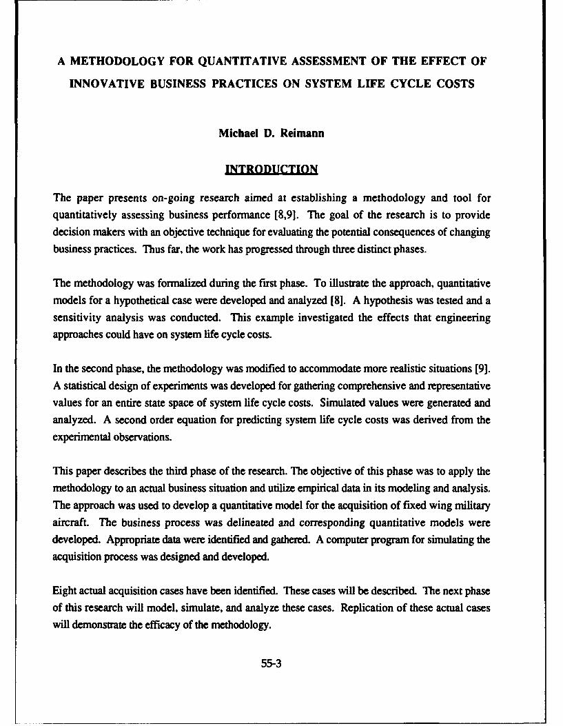
A METHODOLOGY FOR QUANTITATIVE ASSESSMENT OF THE EFFECT OF
INNOVATIVE BUSINESS PRACTICES ON SYSTEM LIFE CYCLE COSTS
Michael D. Reimann
INTRODUCTION
The paper presents on-going research aimed at establishing a methodology and tool for
quantitatively assessing business performance [8,91. The goal of the research is to providedecision makers with an objective technique for evaluating the potential consequences of changingbusiness practices. Thus far, the work has progressed through three distinct phases.
The methodology was formalized during the first phase. To illustrate the approach, quantitativemodels for a hypothetical case were developed and analyzed [8]. A hypothesis was tested and a
sensitivity analysis was conducted. This example investigated the effects that engineeringapproaches could have on system life cycle costs.
In the second phase, the methodology was modified to accommodate more realistic situations [9].A statistical design of experiments was developed for gathering comprehensive and representativevalues for an entire state space of system life cycle costs. Simulated values were generated and
analyzed. A second order equation for predicting system life cycle costs was derived from theexperimental observations.
This paper describes the third phase of the research. The objective of this phase was to apply themethodology to an actual business situation and utilize empirical data in its modeling and analysis.
The approach was used to develop a quantitative model for the acquisition of fixed wing militaryaircraft. The business process was delineated and corresponding quantitative models were
developed. Appropriate data were identified and gathered. A computer program for simulating theacquisition process was designed and developed.
Eight actual acquisition cases have been identified. These cases will be described. The next phaseof this research will model, simulate, and analyze these cases. Replication of these actual caseswill demonstrate the efficacy of the methodology.
55-3

METHODOLOGY
The purpose of the methodology is to provide a general approach for quantitatively assessing
business process performance. This approach is intended to provide decision makers with
visibility into the operating envelop of a business process based on variation of influential
characteristics or drivers. Three aspects are of particular importance in the development of a model
which will reasonably approximate the true performance of a business process:
"* An accurate functional model of the business process.
"• Knowledge of the cost distributions that coincide with the subprocesses composing thebusiness process.
"* Proper identification and characterization of factors that influence process performance.
Using this information, a quantitatively based model of the business process can be derived. From
this model a computer program can be developed for simulating process performance. Then a
statistical experiment can be defined which systematically varies the factor levels in order to obtain
a comprehensive set of experimental observations. These values must be analyzed to insure they
satisfy certain statistical requirements. From the observations an equation can be developed that
establishes a performance envelop for the business process. Operating characteristics of the
process are determined by varying the process drivers. The methodology is composed of the steps
shown in Figure 1.
An overall model of the business process is established and then it is divided into distinct phases.
The phase models are further decomposed into subprocess models. The detailed models of the
various phases and subprocesses are established through a collaborative effort of knowledgeable
people from the host organization. Development of these models is a crucial aspect of the
methodology because the functional components they define will form the basis for a quantitatively
based model of the business process. Preparation of the functional business process model is
indicated by Step 1 in Figure 1.
One or more metrics are established for the ensuing analysis approach. It is necessary to identify
and determine potential changes to the applicable measures for each process phase and subprocess.
Characteristics of these distributions are determined through appropriate and available historical
information and/or estimated when necessary. In addition to the estimates of phase and subprocess
central tendencies, it is necessary to specify the forms of their distributions. Determination of these
characteristics is illustrated by Step 2 in Figure 1.
55-4

Develop a Functional Model of theSystem Life Cycle
O I Determine System Life CyclePhase and Subprocess Costs
) l Identify Important Cost Drivers
4Develop a Quantitatively Based Cost
Model of the System LiUe Cycle4O irTransform the Quantitatively Based Cost Model
into an Equivalent Simulation ProgramTCalibrate Models with an Existing
Operational Example
Adjust Preliminary Models Basedon Calibration Results4
Establish Operational Characteristicsfor an Anticipated Future System
Determine Expermental Design for an
Entire System Life Cycle State Space
[ I Conduct Simulation Experiment,Analyze Data, and Interpret Results
Figure 1 A Methodology for Quantitatively Assessing SystemLife Cycle Processes
55-5

It is also necessary to isolate drivers that influence the performance of each phase and subprocess.
The characteristics of these drivers are determined from historical information, when appropriate.
Otherwise, consensus of opinion by knowledgeable individuals from the host organization is
needed to define and quantify the drivers. This evaluation is shown by Step 3 in Figure 1.
The functional process models developed in Step I serve two purposes. First they establish the
basic relationships between the various phases and subprocesses of the overall business process.
Second, these models identify the type of item that is being manipulated by the phases and
subprocesses. Functional models typically provide minimal information concerning the metric of
interest. Thus, the original functional models are inappropriate for quantification and measurement
purposes. A general input/output model is used to transform the individual functionally based
models into a complete quantitatively oriented model of the entire business process. This
transformation is shown by Step 4 in Figure 1.
Even though the quantitatively oriented process model facilitates communication and
understanding, it is not an appropriate model for implementation on a computer. Therefore it is
necessary to transform the quantitative model into an equivalent representation that can be
simulated by a computer program. This representation is defined as a collection of tabular values.
Internal consistency checks and cross tabulation of the tabular values are used to verify the
quantitative model and the simulation tool. These verifications are indicated by Step 5 in Figure 1.
The performance characteristics of a known business process, which is typical for the host
organization, are simulated through the execution of a computer program. This characterization is
intended to validate the functional and quantitatively based models of the process developed in
Steps 1, 2, and 3. The simulation results should replicate the performance of the known process.Validation and calibration of the preliminary models are shown by Step 6 in Figure 1.
Based on the results of the calibration experiment, adjustments to the functional model, quantitative
model, cost drivers, and/or computer program may be necessary. These corrections are depicted
by Step 7 in Figure 1.
Expected performance characteristics for a new business process or target system are estimated by
knowledgeable individuals from the host organization. As in Step 2, it is necessary to establish
anticipated variation to the applicable measures and drivers for each process phase and subprocess.
55-6

The complete distribution form must be determined for each subprocess. Whenever possible,
consensus of multiple opinion is used to establish these performance characteristics. Determination
of these characteristics is shown by Step 8 in Figure 1.
Statistical design of experiment techniques are used to define a comprehensive set of test points for
characterizing the process. These design points systematically vary the drivers of the businessprocess in an independent fashion. An experimental design defines the appropriate procedures for
assessing a complete state space of process costs. Development of this experimental design is
indicated by Step 9 in Figure 1.
The experiment is conducted to generate simulated costs for the specified design points. These
composite costs are tested to insure that they satisfy necessary statistical assumptions. From these
cost values a mathematical function for predicting performance of the business process can be
derived. The independent variables in this function are the process drivers that were identified in
Step 3. Based on this function, a decision maker can vary the drivers to gain insight into overall
business process performance. The simulation experiment, data analysis, and interpretation ofresults are indicated by Step 10 in Figure 1.
The remainder of this paper describes the development of a baseline model for the acquisition of
fixed wing military aircraft. Steps 1 through 5 of the methodology guided the development of this
model. Subsequent research will employ Steps 6 through 10 to model, simulate, and analyze
actual business cases.
DEPARTMENT OF DEFENSE SYSTEM LIFE CYCLE
The Department of Defense (DoD) system life cycle process for major defense systems is
illustrated by Figure 2 [2,3,111.
Milestone 0 Milestone I Milestone II Milestone III Milestone IV Milestone V
Program Concept IConcept IrEngineering & rdcin& Oertos RtrmnInitrtona Exploration Demonstration Manufacturing IrDatiooment r etiremInitiation & Definition & Validation Development ePly & Support & Disposal I
Figure 2 Department of Defense System Life Cycle Phases
55-7

As shown in Figure 2, this process consists of seven primary phases:
"* Program Initiation
"* Concept Exploration & Definition (CGE)
"* Concept Demonstration & Validation (D/V)
"• Engineering & Manufacturing Development (EMD)
"• Production & Deployment (P/D)
"* Operations & Support (O/S)
"• Retirement & Disposal
Within the DoD, major systems are defined as systems anticipating funding levels of more than
200 million dollars in research, development, test, and evaluation or one billion dollars in
procurement in constant fiscal year 1980 dollars. The process begins by conducting mission area
analysis efforts in determining the user's mission need, followed by an approval for program
initiation and authority to budget for a new program (Milestone 0 decision). Next, the program
normally begins the C/E Phase, during which all reasonable system alternatives are explored. The
program then enters the D/V Phase (Milestone I decision) during which the preferred system
concepts are selected and tested to identify risk areas and to demonstrate that all experimental
efforts have been completed. The results of these efforts are reviewed and the program is allowed
to progress into the EMD Phase (Milestone II decision) where system detailed design and tests are
performed. Once completed, the system is approved to proceed with full-rate production and initial
deployment in the P/D Phase (Milestone m] decision) during which the actual production or
construction takes place. The initial deployment also marks the beginning of the O/S Phase. A
review will be conducted one to two years after initial deployment to assure that the operational
readiness and support objectives are being achieved (Milestone IV decision). Later, during the O/S
Phase, modifications and product improvements are usually implemented. Another review will be
conducted five to ten years after initial deployment (Milestone V decision) to determine if major
upgrades are needed.
At the end of each phase the need for the program is recertified, using milestone decision reviews,
by the Secretary of Defense (SECDEF) or the Service Secretary, as required, before additional
resources are authorized. At each review, the decision authority can choose to continue the presentphase, proceed to the next phase, or cancel the program. The SECDEF can also direct a DoDprogram to omit C/E or DIV phases and proceed to EMD Phase as special circumstances prevail.
55-8

A modified approach, unique to each service, is employed for non-major or non-developmental
systems. Non-major systems may not follow all of the acquisition phases that major systems do.
They will, however, have a development and review cycle appropriate to the nature and scope of
the program. Acquisition of non-major systems is directed by the service or major command, as
appropriate. Each service has its own system of reviews and approvals that achieves objectives
similar to the DoD system life cycle process.
DATA
An essential factor, in this research, is the need for appropriate and accurate data. Preliminary
work in the development of the methodology [8,91 indicated that reliable results are highly
dependent on the cost distributions used. The data for this research were obtained from the United
States Air Force Cost Estimating System (CES) [1]. The CES was developed in 1987 and
contains acquisition data for Air Force, Army, and Navy aircraft purchased between the years 1948
and 1987. These data represent 238 billion dollars in expenditures for 415 aircraft lots. The CES
provides a single comprehensive source of data for these aircraft systems.
Data Partitioning and Categorization
Acquisition of major weapon systems specifically addresses three of the seven DoD system life
cycle phases:
"• Concept Demonstration & Validation (D/V)
"* Engineering & Manufacturing Development (EMD)
"* Production & Deployment (P/D)
Because the CES delineates data at an acquisition lot level and not at an individual aircraft unit
level, the partitioning, categorization, and classification of data used in this research were oriented
at the acquisition lot level. There are fifteen basic cost categories associated with each of the three
system life cycle phases in the acquisition process. Each of the basic cost categories is further
subdivided into non-recurring and recurring cost categories. Non-recurring costs are those which
occur on a one-time basis. Recurring costs are accumulated on a periodic basis. Since each of the
fifteen basic cost categories could have both a non-recurring and a recurring component, there are
potentially thirty cost categories for each of the three phases in the system acquisition process.
Each acquisition lot was examined to determine the phase(s) to which it belongs. Then, all of the
individual costs associated with each of the lots were assigned to appropriate acquisition process
55-9

cost categories. Table 1 summarizes the assignment of lots to the three acquisition phases andninety cost categories in the system life cycle. The counts shown in each cell of Table 1 represent
the number of systems that have non-zero acquisition costs associated with that cost category. Theobserved values for each cell were used to construct an individual cost profile (i.e. cumulativedensity function) for the cost category. In order to construct a cumulative density function it wasnecessary that a cell have five or more observations. Twenty-one of the ninety cells shown in
Table 1 could not meet this criteria and were eliminated from further consideration.
Data Normalization
The CES utilizes the 1987 DoD inflation index to normalize the cost data for price level variationswhich occur over time. Using inflation indices to synchronize costs permits comparisons based on
constant dollars; however, system costs can vary considerably in terms of overall acquisition cost
or unit costs. These differences may be attributed to a variety of factors such as aircraft
sophistication, economies of scale, or learning curve phenomena. Because of these differences,
comparisons among system types, or between purchase lots within a system type, may not be
reasonable or feasible.
To overcome the above noted deficiencies, it was necessary to normalize the dollar amounts into a
consistent unit of measure. This unit is expressed as the proportion of a categorical cost in a lot
relative to the total cost of the lot. The total lot cost is the sum of all the individual categorical costsincurred by the lot. Each of the individual costs categories within the lot is then divided by the total
lot cost to establish its percentage of cost contribution to its lot.
By expressing costs as proportions, inflation no longer affects the individual lots. Therefore, it isnot necessary to index the data to a specific year.
The magnitude of acquisition costs is eliminated when the costs are transformed into percentages.
It is feasible to compare lots which have different acquisition quantities or where the per unit cost
of the aircraft differ. Strict normalization of the data into percentages does, however, remove theability to investigate the effects of economies of scale or learning curve phenomena.
Comparisons among different system types (i.e. F-16 versus F-18) are feasible when the costs are
expressed as proportions of total lot acquisition cost. System classes (i.e. bombers versesfighters) can also be compared in this fashion. Benchmarking of aircraft manufacturers (i.e.
Lockheed versus industry norm) can be conducted once the data were normalized into percentages.
55-10

m'C' m'c~' m- ~ N N Cwc YC
.2
* - V- V- -- V -- - - V- -
ada
oC4 Nm co co o m 0 q~ , q)"
C0cc go
F .
adN
0.
V- - V- - - - - - - - - - - - - 0
?A
cc 00 C- c" ~ Oa. CL
CL
00
* 0
-r- S
0
16.~
oI 0. 0ccc c a
Ca 0
c55-1
Cumulative Density Functions
The final manipulation of the acquisition cost data was to transform the data into a computer
compatible form. The data in each of the sixty-nine cost categories were convened into cumulative
density functions. These conversions involved three steps:
"* The observed values in each cost category were sequenced into ascending order.
"• An empirical distribution function was determined for each cost category.
"* A one hundred step cumulative density function (i.e. ogive) was derived from thedistribution function for each cost category.
The discrete cumulative density functions were implemented as a collection of tabular data which
can be interpreted by a computer simulation program. Graphs of the cumulative density functions
were also generated so their characteristics could be visually examined and interpreted. Figure 3
shows one of these graphs.
1.00
.75
so
.2S
0.00
0.00 10.00 20.00 30.00 40.00 SO.00 60.00 70.00
PROOUCTION AN DEPLOYMET RECURNG MANUFACTrLRNG
Figure 3 Cumulative Density Graph of the Percentage of Acquisition CostAttributable to the Production and Deployment Phase
Recurring Manufacturing Cost Category
55-12

DEVELOPMENT OF A QUANTITATIVELY BASED COST MODELOF THE DEPARTMENT OF DEFENSE ACOUISITION PROCESS
Data for this research were obtained from the Cost Estimating System (CES). Since the CESprovides cost data only for the acquisition segment of the DoD system life cycle, the scope of thisresearch was limited to the three phases of this segment. Figure 4 shows the conceptual
relationship among various components.
Acquisition Phases
Milestone I Milestone 11 Milestone Ill Milestone IV
Concept IEngineering & Prdcto &T Demnonstration Manufact iring PrdcIo && Validation IDevelopment Deployment I
Adhity.................odd.........
........... .......U.
Historicaodutio Acusto&ot
Figure 4Inegratonstatof a Fuctoal odl it CstDaa o roucQuantitatVelyiBatied MDeel ofph o custo rcs
..... m eri .........3

A narrative description of the acquisition segment was translated into equivalent activity based
diagrams. The activity based models were defined so they coincide with the cost categories on a
one-to-one basis. The data were transformed from a dollar basis into proportions that were
consistent within and among acquisition lots. Synchronization of the activity based models with
the normalized values produces a quantitatively based model of the acquisition process. This
synthesis is shown as the shaded region in Figure 4.
The model illustrated in Figure 5 was used to combine the description of the acquisition process
with the CES data to produce quantitatively oriented models of the subprocesses. The input to a
system life cycle subprocess is indicated by the arrow entering into the outer rectangle from the left
hand side. When an item is initially processed, it incurs a one-time non-recurring cost associated
with that subprocess. The cost added to the item is determined from a non-recurring cost profile
curve (i.e. cumulative density function) that coincides with the subprocess.
Process Characterization
System Life Cycle Suprocess
Figure 5 A General Model for Integrating Subprocess Activity ModelsWith Cost Profile Data to Form Quantitatively Based Models
55-14

After the item has completed the non-recurring activity of the subprocess, it may then undergo a
cycle of recurring subprocess activities. The cost added by each cycle is determined from a
recurring cost profile curve (i.e. cumulative density function) defined for that subprocess. After a
predetermined number of recurring cycles are performed, the total cost for the subprocess is
established by combining its non-recurring cost with the sum of its individual recurring costs.
The arrow entering the subprocess from the top is used to alter the performance characteristics of
the subprocess. Changes in process characterization correspond to variations in important
business factors or drivers. Process characterization is used to alter the cost profiles or change the
number of recurring cycles executed. The specific implementation of process characterization
depends on the system characteristic under investigation and the influential factors that drive the
business process.
The general model shown in Figure 5 was used to integrate and combine the sixty-nine cost
categories which compose the acquisition portion of the DoD system life cycle. From a technical
standpoint, the entire model is referred to as a network model. The visual models developed to this
point were primarily used as a way to communicate concepts and ideas among individuals familiar
with the business process and its data and model builders. Once the network model was finalized,
it was then converted into a simulation program.
MODELING AND ANALYSIS OF EIGHT EMPIRICAL BUSINESS CASES
Based on documentation searches at the Aircraft Systems Command Cost Library and interviews
of Air Force Financial Management personnel, no analyses could be identified which assess the
entire Department of Defense (DoD) acquisition process or that utilize a comprehensive set of cost
estimating data. Quantitatively based analyses performed by the Air Force investigate small
subsets of available data which are constrained to limited portions of the acquisition process.
The current research converted acquisition cost values from the Cost Estimating System (CES) into
percentages in order to obtain a uniform and consistent metric. The transformed values enable
comparisons among and within lots, even though the lots may differ due to aircraft classification,
aircraft type, lot size, acquisition year, or acquisition cost. With the transformed values it is
possible to quantitatively investigate high level issues which were previously infeasible to assess.
55-15

Eight actual systems acquisition cases have been identified for investigation. These cases are
concerned with high level issues of the acquisition process. Analyses of these cases will provide
new information from which useful insights can be gained. The time available for the current
research did not permit the modeling, simulation, or analysis of theses cases. Subsequent research
will investigate these acquisition cases. Each of the eight actual cases will be briefly described.
Cost Profiles of Fixed Wing Aircraft Aequisitions
The cumulative density functions of the sixty-nine cost categories enable comparisons of
proportionate aircraft cost within cost categories. Graphs of the cumulative density functions will
be examined to gain insight into the characteristics of cost distributions within individual cost
categories. The categorical cost data will be analyzed using statistical techniques to determine if the
data follow conventional theoretical distribution forms. These statistical tests will ascertain if
theoretical distributions can be used to replace the cumulative density functions. The cost data
within the categories will also be analyzed using mathematical modeling techniques. Curve fitting
of the data will attempt to find reasonable mathematical approximations of the cumulative density
functions. The outcomes of the statistical and mathematical analyses have important implications.
If the actual cost data cannot be reasonably approximated by theoretical statistical distributions or
with conventional mathematical functions, then analytical approaches which rely on these
assumptions will most likely produce erroneous results. Results obtained from analytical
approaches can be compared to simulated results. Because the simulation approach utilizes data
which constitute an empirical population, its results can be used to validate (or invalidate) the
results obtained from analytical approaches.
Comparisons Among Acquisition Costs Categories
Comparisons among acquisition cost categories are possible because the costs have been
normalized into percentages. A profile of aircraft acquisition costs will be developed from the
sixty-nine cost categories which comprise the acquisition process. Graphical techniques will be
used to compare and contrast the various costs that contribute to total acquisition cost. Statistical
comparisons of the data will be made provided the data do not violate assumptions for linearity,
independence, normality, and homoscedasticity.
55-16

Comnarisons of Acguisition Costs Among Fixed Wing Aircraft Classes
This analysis will investigate differences among broad classes of aircraft. The analysis will be
limited to the Production and Deployment Phase of the system life cycle. There are 367
acquisition lots in this phase. The acquisition lots will be segregated into the following eight
mutually exclusive aircraft classes:
" Anti-Submarine Warfare Aircraft - 24 lots
"* Attack Aircraft - 81 lots
"• Bombers - 17 lots
"• Cargo Aircraft - 18 lots
"* Electronic Warfare & Surveillance Aircraft - 31 lots
"* Fighter Aircraft - 181 lots
"• Tanker & Refueling Aircraft - 6 lots
"* Trainers - 9 lots
Cost profiles will be developed for each of these aircraft classes. Twenty-seven acquisition cost
categories compose the Production and Development Phase. These cost categories will be
contrasted and compared among the eight aircraft classes.
Analvsis of Fighter Aircraft Acquisition Cost Trends
The aircraft acquisitions used in this research occurred between the years 1948 and 1987. This
analysis will examine changes in the proportions of acquisition costs among cost categories during
this time frame. Although all three phases of the acquisition process will be considered by this
analysis, it will only include 206 fighter aircraft lots. The lots will be segregated according to their
year of acquisition. The forty year period will be divided into four ten year segments:
* 1948 through 1957 - 54 lots
* 1958 through 1967 - 48 lots
* 1968 through 1977 - 67 lots
* 1978 through 1987 - 37 lots
Cost profiles will be developed for each of these acquisition segments. The sixty-nine acquisition
cost categories will be contrasted and compared among the four time segments.
55-17

Benchmark Analysis of a Fighter Aircraft Manufacturer
Fighter aircraft lots which were acquired for the Production and Deployment Phase will be
extracted from the original 415 acquisition lots. There are 181 lots in this subset. These lots will
be segregated into two groups. One group will contain all the lots that were produced by a specific
aircraft manufacturer. The remaining acquisition lots will form the other group.
Cost profiles for both groups of aircraft manufacturers will be developed. There are twenty-seven
cost categories in the Production and Deployment Phase of the system life cycle. These categories
will be contrasted and compared between the two manufacturer groups.
Cause and Effect Analysis of B-I Bomber Costs
The acquisition costs for the B-1 Bomber were exceptional and extraordinary. Extreme differences
in cost proportions between the B- I and other bomber types will be isolated. A root cause analysis
will be conducted to ascertain why these differences exist. This analysis will be limited to
Production and Deployment Phase acquisition lots. Because only five B-I Bomber lots were ever
acquired, there are insufficient data to make inferences.
Analysis of the Effect of Congressional Appronriations on Acquisition Costs ofthe F-16 Fighting Falcon
The system life cycle for aircraft programs typically span several decades. Funding needs for these
systems are planned several years in advance of their actual expenditure. Congressional
appropriations of funds are made on a yearly basis. Appropriated funds may or may not coincide
with planned outlays. In cases where the actual funding level differs from the anticipated funding
level, program budgets must be adjusted to accommodate the difference in funding levels.
When appropriated funds are less than the funds requested for an acquisition, the production
quantity must be reduced or the acquisition schedule must be elongated. Evidence suggests that
system life cycle cost will increase when the acquisition schedule is extended. The cause for this
increased cost is additional recurring costs that are incurred over a longer acquisition time frame.
An actual case from the F-16 program will be modeled, simulated, and analyzed. Replication of
the F-16 case will demonstrate the efficacy of the methodology.
55-18

Analysis of the Effect of Large Scale Program Reductions on the Unit Cost of theB.2 Stealth Bomber
The B-2 Stealth Bomber has been a closely guarded secret since it was originally conceived. The
existence of the B-2 was only made public a few years ago. Expenditures on the B-2 for research,
development, test, and evaluation have been very high when compared to other aircraft types.
During the past several years, the B-2 program has experienced severe cutbacks in funding. At the
present time, it is expected that the number of B-2 aircraft actually produced will only reach a
fraction of the volume originally anticipated. Funds previous spent on the B-2 program must be
allocated to a much smaller number of aircraft. Consequently the unit cost of the B-2 has risen
dramatically.
This analysis will model and simulate the business situation experienced by the B-2 program. The
B-2 case represents a radical departure from the typical fixed wing aircraft acquisition process.
Replication of the B-2 acquisition case will not only demonstrate the efficacy of the methodology,
it will also demonstrate its robustness to extreme changes in business practice.
SUMMARY AND CONCLUSIONS
This paper gave an overview of on-going research aimed at establishing a methodology for
quantitatively assessing business performance. A brief description of the methodology was
provided. The majority of this paper described the application of the methodology to an actual
business environment. The methodology was used to develop a quantitative model of the
Department of Defense (DoD) process for acquiring major weapon systems. An activity based
model of the process was developed. A comprehensive set of data were obtained for forty-one
DoD aircraft systems. These data underwent various transformations to make them consistent
within and among lots. The activity based model was combined with the normalized data tc form a
quantitatively based model of the aircraft acquisition process. This model was converted into a
computer simulation program. The work conducted during the current research was guided by the
first five steps of the methodology. These steps constitute problem formulation and model
development. The current research demonstrated that business processes can be modeled and
simulated.
The last five steps of the methodology could not be performed in the time available for the current
research. It is necessary to conduct the remainder of the methodology on one or more cases in
55-19

order to demonstrate its viability and applicability to actual problems. Eight business cases were
identified and described. The first six cases do not need the entire methodology to conduct the
suggested analyses. These cases only require manipulation and analysis of the normalized data.
The following two business cases will utilize the remaining methodological steps to complete their
modeling and analyses:
"* Analysis of the Effect of Congressional Appropriations on Acquisition Costs of the F- 16Fighting Falcon
"• Analysis of the Effect of Large Scale Program Reductions on the Unit Cost of the B-2Stealth Bomber
One of these two cases will be modeled and analyzed in order to demonstrate the efficacy of the
methodology.
REFERENCES
[1] Cost Estimating System - Volume 2 - Aircraft Cost Handbook. Delta ResearchCorporation, Arlington, Virginia, November 1987.
[2] Department of Defense Directive (DoDD) 5000.1, Major and Non-Major DefenseAcquisition Programs, September 1, 1987.
[3] Department of Defense Instruction (DoDI) 5000.2, Defense Acquisition ProgramProcedures September 1, 1987.
[4] Engwall, R.L., Managing Investments Strategically, Journal of Cost Management for theManufacturing Industry, Volume 1, Number 3, Fall 1987, pp. 56-58.
[5] Engwall, R.L.. Cost/Benefit Analysis, Journal of Cost Management for the ManufacturingIndustry, Volume 2, Number 3. Fall 1988, pp. 64-70.
[6] Hayes, R.H., Garvin, D.A., Managing as if Tomorrow Mattered, Harvard Business Review,Volume 60, Number 3, May-June 1982, pp. 71-79.
[7] Kaplan, R.S., Must CIM be Justified by Faith Alone, Harvard Business Review, Volume 64,Number 2, March-April 1986, pp. 87-95.
[8] Reimann, M.D., Huq, F., Using Activity Based Costing to Define a Quantitative ProductLife Cycle Cost Model for Concurrent Engineering, in the Proceedings of the ThirdInternational Conference on Flexible Automation and Information Management,Limerick, Ireland, June 28-30, 1993, pp. 485-496.
[9] Reimann, M.D., Whiteside, M.M., Creating an Experiment Design for Assessing theEffects of Concurrent Engineering on Product Life Cycle Cost , in the Proceedings of theThird International Conference on Flexible Automation and Information Management,Limerick, Ireland, June 28-30, 1993, pp. 473-484.
[10] Shumaker, G.C., Integrated Product Development Straw .y., Concurrent EngineeringOffice, Manufacturing Technology Directorate, Wright iesearch and DevelopmentCenter, Wright-Patterson Air Force Base, Ohio, July 1990.
[11] Technical Management Department, The Systems Engineering Management Guide,Defense Systems Management College, Fort Belvoir, Virginia, January 1990.
55-20

A Comparison of Biasing Options in the Laser Multiphoton Ionization Detection ofMethyl Radicals in a Filament-Assisted Chemical Vapor Deposition Reactor
David A. DolsonAssistant Professor
Department of Chemistry
Wright State University3640 Col. Glen Highway
Dayton, OH 45435
Final Report for:
Summer Faculty Research ProgramWright Laboratory
Aero-Propulsion and Power DirectorateWright-Patterson Air Force Base
Sponsored by:
Air Force Office of Scientific ResearchBoiling Air Force Base, Washington, D.C.
and
Wright LaboratoryAero-Propulsion and Power Directorate
Wright-Patterson Air Force Base
September, 1993
56-1

A Comparison of Biasing Options in the Laser Multiphoton Ionization Detection ofMethyl Radicals in a Filament-Assisted Chemical Vapor Deposition Reactor
David A. DolsonAssistant Professor
Department of ChemistryWright State University
Abstract
An apparatus and procedures were developed for the detection of methyl radicals in a filament assisted
chemical vapor deposition reactor operating with methane/hydrogen gas mixtures similar to those used in the
generation of diamond-like carbon films. The apparatus was designed to detect small transient currents as the
focussed output of a tunable dye laser ionizes methyl radicals between a hot filament and a deposition substrate.
The current design incorporates the use of an electrode pair for ion collection, that may be translated between the
filament and substrate. Results from two circuit designs with different bias geometries for ion collection are
presented.
56-2

A Comparison of Biasing Options in the Laser Multiphoton Ionization Detection ofMethyl Radicals in a Filament-Assisted Chemical Vapor Deposition Reactor
David A. Dolson
INTRODUCTION
There is general agreement from modeling results and from experiments that the methyl radical (CH3 ) is
one of the "growth species" linked to the transport of carbon to the substrate where diamond growth occurs in
filament assisted chemical vapor deposition (CVD) of diamond-like carbon films.' Quantitative measurements of
[CHj.I using resonance enhanced multiphoton ionization (REMPI) allows for a degree of spatial resolution because
ions are only created in a small focal volume. Celii and Butler2 have used the REMPI 3 technique to measure the
relative CH3 concentration in a filament-assisted diamond CVD reactor as a function of several process parameters.
In their application an ion collector wire was fixed 4 mm above the substrate surface, the laser focus was
approximately midway between the wire and the substrate, and the filament position was varied in order to probe
the spatial [CH 3-] profile.
This report describes the development of a REMPI detection experiment for methyl radicals that is designed
for spatial profiling of [CH 3.] in a fixed gap between the filament and substrate. This design avoids changing the
filament-to-substrate gap as the spatial profiling is accomplished. Preliminary results are presented, and suggestions
are made for continuing efforts.
APPARATUS and PROCEDURES
The filament-assisted CVD reactor was constructed from heavy-walled 4.5 inch O.D. glass pipe. The reactor
was constructed in two sections, connected with an o-ring seal. Its overall length was -18". Kovar rods, sealed
through the top section of the reactor, were used to power the filament and give it support. A short section of glass
rod held the tips of the kovar rods apart by -25 mm and provided an anchor for supporting the center of the
filaments. A 1" dia. port centered in this section allowed for the introduction of mixed gas flows through a 0.5" dia.
pyrex tube at selected distances from the filament.
56-3

The length of the kovar rods was such that the filament was located -5 cm inside the other section when
the reactor was assembled. This section (the main body of the reactor) held the windows for passing the laser, the
pressure measurement and vacuum ports, and the introduction port for a linear translator for the biasing and
collection electrodes. The vacuum port was mounted to an aluminum plate for connection to a pressure control
throttle valve. Flexible tubing connected this valve to the 400 m3 hr" booster pump, which was backed by a 60 m3
hr" two-stage rotary pump.
Typical coiled filaments were constructed using nine turns (-5 mm dia coils) of a 0.010" dia. tungsten (G.E.
"218") wire which was attached to the Kovar rods by winding the free ends of the wire around the rod a few times
and securing it with an alligator clip. Some filaments were more simply made from a straight length (-25 mm) of
wire. The center of each filament was supported from the glass connecting rod by the use of a loop of the tungsten
wire. The filament was heated by adjusting the current slowly to approximately 8 amperes, and the filament
temperature was monitored with a hot filament pyrometer. A 200 sccmn gas flow of 2% CH, in H, was caused to
flow over the filament toward the substrate 7-14 mm away and on to the pumping port at the far end of the reactor.
Gas flow rates were measured with electronic mass flow controllers, and total pressure was measured with a
capacitance manometer with a 10 torr full scale rating. The substrate was a 1" dia x 0.1" thick molybdenum disc
in the current work. The substrate was not connected electrically in the first circuit design (Fig. 1) to be described
in this report. In the second design (Fig. 7) the substrate was electrically grounded.
In a previous circuit design using only a filament and substrate, it appeared that the collection efficiency
for laser-generated ions was a function of the bias voltage used to control the discharge current. In an attempt to
overcome this undesirable effect, a pair of kovar rod (0.060" dia) electrodes were mounted on a linear translator for
movement between the filament and the substrate. In the first circuit design (Fig. 1), one rod was biased and the
other was connected through a load resistor (1820 or 4090 ohms) to electrical ground. In the second circuit design
(Fig. 7), both electrodes were tied together and connected to ground through the load resistor. Transient REMPI
signals were detected as a voltage generated across the load resistor and passed through a capacitor to a digital
oscilloscope (1 Mfl AC input impedance) for summed averaging over 100-1000 laser shots. Most often, peak
REMPI signal levels were recorded and plotted; however, the time duration of the signals decreased at higher bias
56-4

New Circuit with Double Probes
SorensenSupply
30V
SrFilamentShn
0 •Computer1820 Ohms
"to
Substrate 250uF OscilloscopeHolder
Inductor
- +I
0-300V
FIG. 1. Circuit design with bias and collector electrodes.
56-5

voltages and lower pressures. Consequently, a somewhat different view of the data (larger signals at lower voltages
and higher pressures) is obtained by using integrated REMPI signal intensities (see Fig. 10). Unfortunately, the large
amplitude electromagnetic interference generated at the time of the excimer laser firing overlapped the expected time
for collection of photoelectron current. CO .:quently, the REMPI signals observed in this study are attributed to the
movement of molecular ions.
REMPI signals were obtained by scanning the tunable output of an excimer-pumped dye laser (Lambda
Physik EMG-103MSC/FL2002) near the 333.5 nm transition for methyl radicals and near 339.4 nm for methyl
iodide. The dye laser delivered up to 8mJ/pulse at 333.5nm using a p-terphenyl/p-dioxane dye solution pumped at
248 nm with a KrF excimer laser. It was common for the laser power to decrease significantly by 1-2 mJ/pulse over
the course of some of the longer experiments. No power correction has been made for any of the data presented
here. Most of the current work was done with the laser operating at 10Hz. The laser was focussed between the
electrodes with a 20 cm focal length lens. The vertical and horizontal positions of the laser could be adjusted
externally with turning prisms mounted on linear tranlation stages. Filament, substrate, and electrode positions were
determined by moving the laser beam until contact was determined visually by the spark generated.
RESULTS and DISCUSSION
The first evaluation of the circuit design with bias and collector electrodes (Fig. 1) was made using a 2%
methyl iodide/hydrogen gas mixture at 10 Torr because of the ability to generate uniform concentrations with a stable
species. The filament was cold for these evaluations. Fig. 2 presents a time-resolved REMPI signal observed for
methyl iodide with a +150 volt bias on the one electrode and the filament biased at +27 volts to simulate the
potential of a hot filament. This observation is the difference of 200 laser shots "on resonance" (at the peak near
339.4 nm) and 200 laser shots "off-resonance" (at 338.0 nim). The time-scale for observations such as this ranged
from -25 ps at 300 volt bias to -200 ps with no bias.
The results for various combinations of filament and bias potentials are presented in Fig. 3. The results are
qualitatively as expected. The positive potential sends positive ions to the (grounded) collector and attracts electrons
(and/or negative ions, if present) to the biased electrode. The current generates a positive voltage drop across the
56-6

C
- L 0-
-. <I..
• -- - 1 I j' ~ - ! - • i I Vl ! i -. -
' 0--I'
-6
I -- ,ca,
56-7

C',
-0
C)ca
0
U)
4- -
0) C
CM c
*0 c0 co
w-0r
U) Cl) C
7F 7E U .
> 0 0 >> > ___ __ _ 0 cr5
N - fl - N
56-8

load resistor. Negative potentials generate negative polarity signals due to the reversed current direction. The
increasing magnitudes of the slopes of the curves at the higher potentials is consistent with secondary ionization by
accelerated photoelectrons. The actual collection of electrons is estimated to occur within 2 ps of the laser pulse'.
the drift time of the ions being much longer. The electron collection period is obscured by the electromagnetic
interference (EMI) caused by the excimer laser pulse. Thus, most of the signals collected during this study are
attributed to ion currents. Methyl radicals were generated in a 2% methane/hydrogen gas mixture using
tungsten filaments operated at typical temperatures of 1800-2000°C. The methyl radical REMPI signals are presented
in Fig. 4 as a function of bias voltage and electrode micrometer readings. True distances from the filament are 2
mm greater than the stated micrometer readings. The filament potential ranges from ground at one side to -31 volts
at the other side, and the filament temperature was 1970'C. The laser energy was 3 mJ/pulse, and the on- and off-
resonance wavelengths were 333.5 nm and 333.0 nm, respectively.
The contrasting behavior (compared to Fig. 3) of the methyl radical REMPI signals is immediately apparent.
Near the filament the peak REMPI signals are quite strong when no potential is applied to the collection electrodes,
and the maximum signal occurs at -10 volts potential. The signal falls off rapidly as the potential is made
increasingly negative. At +10 volt potential there is still a net negative signal, although it is of interest to note that
the off-resonance signal was entirely positive. REMPI signals are more difficult to detect at more positive potentials.
There is no opposite polarity similarity for the methyl radical REMPI signals as there was in Fig. 3 for methyl
iodide. The same qualitative behavior with respect to potential was observed at 5mm and 9mm micrometer readings
but with reduced intensity in keeping with the expected reduction in methyl radical concentration away from the
filament.
Futither investigation of methyl radical REMPI signals as a function of distance from the filament gave
results similar to those depicted in Fig. 5. Peak signals were always greater (negative polarity) near the filament,
falling off as the laser focus and collection electrodes were translated toward the substrate (14 mm filament-to-
substrate gap). This behavior is in agreement with the expectation of [CH 3.] reduction away from the filament
confirmed in other studies"s. The occurrence of larger REMPI signals at lower collection potentials is demonstrated
again in this figure.
56-9

0
00
E E EE E E4-
0 LO (D
(Du
CA
ca*0 a
0.)
LI-
C13
56-10

-2- 25 ýorr ___ ___ ___ ___ __ ____
-~-6-______
I0-.
-12-Liicc -14--0Vot
~ 16--3Vot
-18-- _00_olt
0 1 2 3 4 5 6 7 8 9Micrometer reading
~0
9wor I
04-)28Vot
-i- -100 Volts
0 1 2 3 4 5 6 7 8 9Micrometer reading
FIG. 5. Methyl radical REMPI signals as a function of distance from the filament.True distance is obtained by adding 2 mm to the micrometer reading.
56-11

During the course of this work, it was observed that the DC current through the load resistor increased,
under certain biasing conditions, with increasing temperature and decreasing filament-to-electrode distance. Large
DC current levels proved to suppress the REMPI signals, as shown in Fig. 6A, where peak REMPI signals and DC
current are plotted versus electrode distance from filament. When the electrodes were within 4 mm of the 2020"C
filament, the DC current was in excess of 0.5 mA, and the peak REMPI signals jumped to lower values. At the
lower 1940°C filament temperature the DC current was not excessive, and the REMPI signal levels increase nearer
to the filament (in agreement with the expectations of Fig. 5).
A further demonstration of this effect is demonstrated in Fig. 6B, where the REMPI signals (mV) and the
resistor voltages (V) are plotted versus filament temperature for the 2mm electrode position. The equivalent DC
current is 0.5 mA at -2 volts across the load resistor. Here, again, the peak REMPI signal suffers reduction when
the filament temperature reaches a point where large currents are picked up by the collector electrode. This behavior
was not noted in other studies-' where the methyl radical REMPI signals (electron current) increased with
temperature up to a nearly constant value between 2200°C and 2500°C.
Near the end of this study we modified the circuit design of the apparatus to closely reproduce that reported
by Corat and Goodwin5 in a recent publication. This design, presented in Fig. 7, grounds the substrate and
incorporates an additional power supply to maintain a constant potential difference between the filament and the
paired collection electrodes (20 volts more positive than the low side of the filament). The filament-to-substrate gap
was 7-9 mm, depending upon the filament placement, for all of this work. Corat and Goodwin5 showed increasing
REMPI signals from 0-50 volts electrode bias, and they were able to obtain saturated electron collection conditions
over the range of 50-150 volts electrode bias (their figure 3). REMPI signals were obtained as a function of bias
voltage (Fig. 8), distance from the filament (Fig. 9), and total pressure (Fig. 10) in the present study.
REMPI signals as a function of electrode bias voltage were obtained with the collection electrodes and the
laser focus positioned 4 mm above the grounded substrate (-3 num from the filament). The laser beam was parallel
to the electrode rods in this study whereas the beam traveled perpendicular to the single collection electrode in the
apparatus of Corat and Goodwins. The squares in Fig. 8 were obtained with a (coiled) filament temperature of
56-12
,-51.0
o 05 DC Current (A0.
C
C
-5 ~- -
WU Peak REMPI Sig~nal (mV)
.CL- -1 . ....
0 2 4 6 8 10 11
Filament-to- Electrode Distance (m m)
Fig. 6A Methyl radical REMPI signal and DC current as a function of electrode position.* points were obtained with TMi2020'C (32.6 V 0 8.0 A) first.* points were obtained with T61=1940 0C (30.7 V @ 8.0 A) after the first set.
Laser pulse energy was 4.8-4.9 mJ, and the collection potential was -32 V.
2-
-CD Methyl Peak Voltageg ;__ -4-Resistor Voltage
S-6
CM
05 10
(D
-14.
1650 1750 1801950Filament Temperature (C)
FIG. 61 Methyl radical REMPI signal and D.C. voltage across load resistor as a function of filamenttemperature.
56-13

Fig.7 Circuit design with constant potential between filament and collection electrodes(similar to Goodwin's design)
SorensenSupply
30V
Filament Shuntb
Computer
4k Ohms•' ~~ '•10pF
toOscilloscope
SubstrateHolder-_
Sorensen
20VSRS
__0-150V"---- 56-14
0
(D
L E
CvCM
I•. o3 O3
caCJ oi
0)
CIS
0
0'
a)
S° C
(D i
.CD
CMO
LO in) OI--4 c
(sp~un " Pe)lUBIS IdVG8• IA419IN
56-15

0-25 Torr
-2 -_--
C.4 _ __ _ _ _
0a -264 68a -8
-10-
w -1
"-14 , -! -- 70 volts
-16 110 ,,.- - l vo lts
-1 8 . . . T . .. . . . . .0 1 2 3 4 5 6 7 8 9
Distance from Filament (mm)
09 Toi
-2/Cn
-4-
CD(I,
- -70 Volts
2 10\/ -- e-l Volts-14 2.
0 1 2 3 4 5 6 7 8 9
Distance from Filament (mm)
FIG. 9. Methyl radical REMPI signals as a function of distance from the filament.True distance is obtained by adding 2 mm to the micrometer reading.
56-16

0-_ _ _ _ _ _
-10-1
-20 --m ekSga
E-ja -30- _____
C
5, -40 - ______
-50
0 5 10 15 2 0 25Pressure (Torr)
0-
C/)
-3-
0 5 10 15 20 25Pressure (Torr)
FIG. 10. Methyl radical REMPI signals as a function of total pressures.
56-17

-1900°C and 6.5 mJ/pulse laser energy. REMPI signals were reduced by a factor of two or more when the laser
focus was located midway between the collection electrodes and the substrate (Corat and Goodwin's arrangement5 ).
The circles and triangles in Fig. 8 were obtained on a different day with a single strand electrode. T,1= I 8500 C. and
5.2 mJ/pulse laser energy. The 5 mm and 9 mm labels of Fig. 8 are micrometer readings that correspond to 4 mm
and 8 mm distances from the filament. The DC current was less than 0.1 mA for all of the data of Fig. 8. The
REMPI (ion current) signals were not observed to saturate with bias voltage in the manner observed by Corat and
Goodwin' for electron current.
REMPI signals as a function of distance from the filament are more completely presented in Fig. 9. These
data were obtained on two different days using single strand tungsten filaments at 2030*C (top) and 18800 C (bottom)
and two bias voltages (10 and 70 volts) at 9 and 25 Torr total pressures. The laser pulse energies were 5.2 mJ for
the 25 Torr data (top) and 4.3 mJ for the 9 Torr data (bottom). Peak REMPI signals were greater at the lower bias
voltage, and they decayed as the detection point was moved away from the filament. The small decreases close to
the filament are related to the larger DC currents observed at those positions (as in Fig. 6A). The observations of
Figs. 8 and 9, greater REMPI signals at lower bias voltages and decreasing signal away from the filament, are
qualitatively the same as those presented in Figs. 4 and 5 for the previous circuit design.
The observation of larger REMPI signals at lower collection potentials is quite puzzling. It has been
suggested by one author (MDK) that the behavior is suggestive of the presence of negative ions, presumably
produced by attachment of the electrons generated by the REMPI laser pulse. The electron attachment hypothesis
is consistent with smaller cross-sections for the higher collection potentials that yield more energetic electrons. In
fact, calculations6 have shown that dissociative attachment (e- + H2(v) -4 H- + H.-) involving vibrationally
excited H2 can be efficient. Detection of HW produced in pure hydrogen gas flowing over a hot tungsten filament
suggests that the process is more efficient at lower pressures where vibrational deactivation of the H,(v) reactant is
reduced7. In our experiments, however, higher pressures are expected to yield greater methyl concentrations, 0•
source of the electrons to be attached. Thus, there are competitive processes at work that make it difficult to preo.,L.
the pressure dependence of the REMPI signals. Results from an investigation of REMPI signal versus total pressure
of the 2% CHI/H2 gas mixture are presented in Fig. 10. Peak signals and integrated signals are presented. The
56-18

integration limits were from -2 .is to the point where the signal crossed zero as it underwent damped oscillation.
For this experiment the filament was maintained at 1960-1990°C, the electrode bias was 15 volts, and the laser
energy was 6.1 mJ/pulse. The longer time duration of the signals at lower pressure tend to increase the relative level
of the integrated signals at lower pressures. The result is an approximately linear dependence of integrated REMPI
signals with pressure over the range 2-20 Torr, at which point the signal seems to saturate. The DC current collected
by the probe ranged from 0.27 mA at 25 Torr to 0.64 mA at 2 Torr. We do not expect that any significant reduction
of signal occurred at these current levels. While the negative ion hypothesis has some support, there is one
remaining observation that it still does not answer. The almost complete lack of REMPI signal with the positive
collection potentials (Fig. 4) in the first circuit design is yet a mystery. The potentials modeled for the experiments
indicate that ions generated between the electrodes should be detected, and the number of CH3 '* ions should equal
or exceed that of H..; but little or no signal is detected.
SUMMARY and CONCLUSIONS
Methyl radical REMPI signals, with temporal and spatial resolution, were obtained from 2%
methane/hydrogen gas mixtures in a filament-assisted CVD reactor using different collection geometries and biasing
options. Observations were attributed to photo-generated ion currents because detection of transient electron currents
was blocked by laser noise. While the observations of REMPI ion currents in 300K methyl iodide was in qualitative
agreement with expectations, the REMPI signals generated from methyl radicals at 333.5 nm exhibited
unconventional behavior with respect to collection potentials. A hypothesis involving the production of negative ions
by dissociative attachment to vibrationally excited H2 was considered because it was consistent with the occurrence
of larger REMPI signals at lower potentials. The suggestion has been mades that using a photodetachment laser
pulse delayed after the REMPI laser might provide a further test of the negative ion hypothesis.
Because of the uncertainty of the source of the observed REMPI signals with the present detection methods,
we cannot recommend using the present procedures even as a relative measure of methyl radical concentrations in
a CVD reactor. We are confident, however, that quantitative measurements could be obtained by observing the
56-19

electron current generated in the MPI event. This would require efforts at laser EMI noise reduction so that the early
time signals could be obtained with much less interference.
ACKNOWLEDGEMENTS
Ideas and assistance from Dr. Peter Bletzinger were invaluable as were conversations with Drs. Bish
Ganguly and Alan Garscadden. I appreciate the calculation of electron mobilities by Rajish Nagpal and the mapping
of potentials by Peter Bletzinger. The technical expertise and cheerful assistance of Mike Ray and Bob Knight made
this work possible. I acknowledge the assistance of Craig Bartell and Michelle Klingshirn in collecting a significant
portion of the data.
REFERENCES
1. Two reviews of the diamond CVD processes are: P. K. Bachmann; R. Messier Chem. Eng. News, pp 24-38,
May 15, 1989. and F. G. Celii; J. E. Butler Ann. Rev. Phys. Chem. (1991), 42, 643-84.
2. F. G. Celii; J. E. Butler J. Appl. Phys. (1992), 71, 2877-83.
3. J. W. Hudgens; T. G. DiGuiseppe; M. C. Lin J. Chem. Phys. (1983), 79, 571.
4. R. Nagpal, private communication.
5. E. J. Corat; D. G. Goodwin J. Appl. Phys. (1993), 74, 2021-9.
6. A. Garscadden; W. F. Bailey Prog. Astronaut. Aeronaut. (1981), 74(Rarefied Gas Dyn., Pt. 2), 1125-37.
and W. F. Bailey; A. Garscadden Brookhaven Natl. Lab., [Rep.] BNL (1980), BNL-51304, Proc. Int. Symp.
Prod. Neutralization Negat. Hydrogen Ion Beams, 2nd, 33-41.
7. P. Bletzinger, private communication.
56-20

PLIF Images of Supersonic Jet Mixing in theWright-Patterson AFB Supersonic
Combustion Facility
James F. DriscollAssociate Professor
Department of Aerospace EngineeringUniversity of Michigan
312 Aerospace Engineering BuildingAnn Arbor MI 48109
Final Report for the1993 AFOSR Summer Faculty Research Program
Research performed in conjunction with:
Dr. Abdollah S. NejadAdvanced Propulsion Division
Aero Propulsion and Power Laboratory POPT/WLWright-Patterson Air Force Base OH 45433
Sponsored by:Air Force Office of Scientific Research
Boiling Air Force Base, Washington D.C.
30 September 1993
57-1

PLIF Images of Supersonic Jet Mixing in theWright-Patterson AFB Supersonic
Combustion Facility
James F. DriscollAssociate Professor
Department of Aerospace EngineeringUniversity of Michigan
312 Aerospace Engineering BuildingAnn Arbor MI 48109
Abstract
Some experimental measurements are described which resulted from an AFOSRsponsored interaction between Dr. J.F. Driscoll, Dr. A.S. Nejad of Wright-PattersonAFB, and other researchers in the Advanced Propulsion Division. The goal of the workwas to study the mixing of a turbulent jet of gas that is injected coaxially into a supersonicair stream. A unique supersonic wind tunnel facility was used that was developed by, andis currently operated by Dr. Nejad. A circular, underexpanded sonic jet issues along thecenterline of a Mach two wind tunnel. The injector consists of a splitter plate with acircular orifice on centerline; this design simulates a fuel injection strut in a scramjetcombustor, and it was selected because the simplicity of the boundary conditions allow it tobe modelled using existing numerical codes. The jet fluid is he,' -n which is seeded withgaseous acetone. A Planar Laser-Induced Fluorescence (PLIF) imaging system was usedto record images of the acetone fluorescence during the mixing process. Several methodswere considered to reduce the data in order to extract images of the jet mixture fraction (f),which is the fundamental parameter of interest in mixing models.
Images of the mixing process were obtained for three different injection conditionsand for several different imaging locations, including the near field and the far field of thejet. Values of the pressure ratio, defined as the jet exit static pressure to the air staticpressure, were selected to be one, two and five. Results indicate that acetone fluorescenceis a useful method to identify the shock wave structure and to quantify several parametersthat characterize the mixing process. These parameters include the centerline decay of themean mixture fraction, the radial profiles of mean mixture fraction, turbulent fluctuations inmixture fraction, and the eddy structure of the scalar field within the jet. The jet spreadingrate is much smaller for the supersonic cases than, for typical subsonic jet mixing cases.This difference occurs because several additional physical processes are introduced whenthe surrounding flow becomes supersonic, including the effects of velocity ratio, densityratio, and compressibility. The images obtained provide a useful set of data that are beingused to develop general scaling laws for the supersonic mixing process and to improveexisting numerical models of mixing.
The work also revealed that additional research is needed to quantify the pressureand temperature dependence of the fluorescence intensity from acetone at the relatively lowpressures of 0.5 atm. and low static temperatures of 166 K (minus 160 degrees F) thatoccur in the present supersonic airflow. Calibration measurements are needed in acontrolled pressure cell in order to properly reduce all to the data obtained to date. Suchfollow-on measurements will be proposed as a Summer Research Extension Program(SREP).
57-2

-7i
PLIF Images of Supersonic Jet Mixing in theWright-Patterson AFB Supersonic
Combustion Facility
James F. Driscoll
Introduction
The mixing between a fuel jet and a surrounding supersonic air stream issignificantly different from the well-known mixing process that occurs in subsonic jets.Additional physical phenomena are introduced as the surrounding air flow velocity isincreased into the supersonic range. The shear layers in some portions of the jetboundaries are driven by the higher-velocity surrounding air, rather than by the jet itself.The eddy structure is thus altered and the shape of the profiles of the turbulence levels canbe changed. Shock waves occur within the underexpanded jet and other shock waves resultfrom the expansion-recompression process associated with the injector geometry. Suchshock waves tend to alter the vorticity field, due to the production of baroclinic torques anddue to velocity changes induced by the shock waves. It is desired to understand these newphenomena in order to use them to improve fuel-air mixing within scramjet combustors.
In order to optimize the fuel-air mixing process, the Air Force has developed aunique, high quality supersonic wind tunnel at the Aero Propulsion and PowerLaboratories that was designed by, and is now operated by, Dr. A. Nejad and his researchteam. Several novel fuel nozzle designs are being tested in order to achieve enhancedmixing. Concurrently, studies are in progress at the University of Michigan in which arelatively small but versatile supersonic flame tunnel is used by Dr. Driscoll and hisstudents to obtain different, but related, experimental data, such as the blowout limits ofsupersonic hydrogen-air flames [21 and the lengths of supersonic flames [3]. It wasdecided that PLIF images of the jet mixture fraction (f) in the APL facility would be the bestmethod to quantify the supersonic mixing process and to eventually explain the trendsobserved in the supersonic flame data obtained at Michigan.
Experimental Arrangement
The supersonic combustion facility at the Advanced Propulsion Division is shownschematically in Figure 1. Gruber and Nejad [1] provide a complete description of thesystem that is shown. The facility provides variable Mach number capability (from Mach1.5 to 3.0) in the 5-inch by 6-inch test section. The heating and pumping capacity providespeak air flow rates of 34 lbm./sec at stagnation temperatures up to 1660 R and stagnationpressures up to 400 psig. The nominal test section static pressure and temperature for thepresent work were 7.35 psia and 294 R, respectively. Visible and ultraviolet optical accessis provided by windows on three sides and on one end. The system is operatedcontinuously, which is a major advantage, since it allows up to several hundred images tobe obtained in a single run. Another advantage of the facility is that the air can be divertedin order to temporarily interrupt the flow to the test section (to make modifications during a
57-3

run) without shutting down the air supply system or having to cool the heated air supplylines.
The summer research described herein was a study an underexpanded sonic jet ofhelium that is injected along the tunnel centerline. Therefore a horizontal splitter plate wasinserted along the tunnel axis and a 0.635 cm diameter circular orifice was machined at thecenter of the splitter plate. A static pressure tap is used to determine the static pressure atthe jet exit, which is set to values that are one, two or five times that of the static pressureof the air stream.
An acetone (CH3-CO-CH 3) seeder was developed by the research team in order toseed the helium jet fluid with desired concentrations of acetone vapor. Heated helium waspassed upward through a enclosure containing liquid acetone. The acetone concentration isdetermined from the known mass flow rate of helium and the known mass of acetone thatis vaporized per second.
The acetone concentrations were measured using Planar Laser-InducedFluorescence imaging. A vertical sheet of ultraviolet laser light at 266 nm was provided bya Quanta-Ray YAG laser whose output (at 1064 nm) was frequency doubled twice.Acetone absorbs in the broadband region between 225 and 325 nm, and the resultingfluorescence is emitted in the blue region of the visible spectrum. The fluorescenceintensity was recorded using a Princeton Instuments cooled, intensified CCD array camera(PI-ICCD 576) and a Vivitar F2.8 macro lens. The advantages of using acetone to markthe fuel mixture fraction is that it has a high vapor pressure (yielding a mole fraction of upto 0.30 acetone in the jet fluid), it has only mild toxicity and is non-carcinogenic, and it hasa large fluorescence yield.
Data Reduction Procedure
The fluorescence signal was related to the fuel mixture fraction by utilizing thecalibration results of Lozano, Yip and Hanson [4]. They state that "The dominantdeexcitation path for acetone singlets is the intramolecular intersystem crossing to tripletlevels: collisional quenching is negligible, and therefore the quantum yield is independentof molecular collisions, hence independent of temperature and local gas composition. Forconcentration measurements, acetone fluorescence signals are particularly easy tointerpret." As a result of their calibration measurements, they state that "Confirming thetheoretical predictions, no temperature dependence of the fluorescence emission in thetemperature range of these experiments was detected. Neither were appreciable self-quenching, or quenching of the acetone fluorescence by oxygen or nitrogen observed."
The equation for the fluorescence intensity (If) that is used in PLIF studies isobtained by equating the rate of photon absorption to the rates of subsequent emission andcollisional quenching, to yield:
If/Ifo = cI nacet/[ 1 + c2Q(nact n,T)] (I)
where Ifo is the fluorescence intensity at a reference location, nacet is the acetone localnumber density, cI and c2 are constants that depend on the transition levels and the opticalcollection system, and Q is the quenching term that depends on total number density (n),temperature, and nacet. The calibration results of Ref. 4 that are summarized in the
57-4

preceding paragraph indicates that the second term (c2Q) in the denominator of Eq. I can beneglected with respect to unity.
In order to reduce the data, it is noted that Eq. 1 states that the measured intensityratio L110 is proportional to nacet since Q is constant, and thus:
If/Ifo = nacet/naceto = XN n / no (2)
where subscript (o) refers to conditions at the nozzle exit and XN is the mole fraction ofnozzle fluid (helium and acetone) at any location in the jet. We now define the jet fluidmixture fraction (f) as the mass fraction of fluid that issued from the jet and the standardrelation between mass fraction of nozzle fluid (YN) and mole fraction (XN) is used:
f = YN = MNXN/[MN XN + MA (1-XN)]
The molecular weight of air is MA and the molecular weight of the nozzle fluid is MN.Combining the above relations, it follows that:
f = { I + (MA/MN)[(lfo/If)(n/no) - 1] -1
The final step involves eliminating n/no, which equals (PIPN)(TNIT) because of the idealgas law; PN and TN are the static pressure and temperatures at the fuel nozzle exit where Iois measured, thus the result is:
f = ( I + (MA/MN)[(Ifo/If)(p/pN)(TNT) - I }1 (3)
Equation (3) is the relation that provides the fuel mixture fraction (f) at each pixellocation in the images. It is necessary to provide the local gas pressure and temperature(p,T) to reduce the data. This is a requirement of all PLIF studies for which the PLIFsignal has a pressure and temperature dependence, which is nearly always the case. Threemethods to complete the data reduction are described.
METHOD 1: Pitot probe measurements
The ratio p/T required in Eq. (3) can be determined in the first three shock cellsfrom pitot probe measurements on centerline. Each shock cell is observed to be 3 nozzlediameters (dN) in axial length, so three cells extend nine nozzle diameters downstream. Itis known that the gas on centerline in the first three cells must be nozzle fluid only, due toobservations of the shear layers in the PLIF images, and due to images obtained usingRayleigh scattering from submicron water droplets in the air stream. It also has beenshown in previous work that air does not mix to centerline before nine nozzle diameters.The pressure and temperature in the first shock cell also is known from the isentropiccalculations of Adamson and Nicholls [5]. Downstream of the third shock cell, the ratio ofstatic pressure to static temperature (pm is approximately equal to that of the ambientairstream. It is noted that this ratio (pT remains approximately constant across therelatively weak compression and expansion waves downstream of the third shock cellbecause both p and T increase across compression waves and both p and T decrease acrossexpansion waves so their ra ,o is relatively insensitive to weak waves. Therefore Eq. (3)can be used to reduce the ý,ata using the centerline pitot measurements in the first threeshock cells, and and it can be assumed, with no additional loss of accuracy, that the ratiop/T is constant downstream of the first three shock cells.
57-5
METHOD 2: Simultaneous PLIF/Rayleigh scattering images
The Advanced Propulsion Division research team at Wright-Patterson AFB hasbegun to develop a new diagnostic method which utilizes Rayleigh scattering fromsubmicron water droplets in the air stream. The intensity of this signal is denoted IR andthe value of this signal is l.a in the air stream, far from the jeL Thus:
IR/IR~a= nA/nAa =XAn/nAa =(0-XN) (n/nA.a) (4)
where nA is the number density of air in the mixing region, 2nd nA,a is the air numberdensity in the unmixed air stream. Combining Eqs. (2) and (4) allows the number densityof the mixture (n) to be eliminated from the two equations; thus:
f = [ I + (MA/MN)(If.o/If)(IR/IR.a)(PA.a'Po)(ToTrAa) 1-1 (5)
Thus Eq. (5) allows the mixture fraction to be deduced from simultaneous images of theacetone fluorescence (If) and the Rayleigh images of the water droplets (It). Conditionsare known at the fuel jet exit (subscript "o") and in the undisturbed supersonic air stream(subscript A,a). The molecular weight of the nozzle fluid (MN) also is known. It is seenthat near centerline IR will approach zero (no water drops may reach centerline at somelocations), which forces f to approach unity. Radially far away from the centerline thePLIF signal (If) will approach zero, causing the entire term in the square brackets to go toinfinity; thus f approaches zero, which is the correct behavior.
METHOD 3: Pressure and temperature measurements using CARS
The most direct method to measure mixture fraction is to use Eq. (3) and to insertinto this equation the measured values of p and T at each location. Simultaneous images ofp and T would be required, which would require extensive diagnostic capabilities. Singlepoint mean measurements of p and T may be adequate, but further research is needed todetermine if the errors associated with using the mean values of p and T, rather thaninstantaneous values, would make this approach worthwhile.
Results
Figure 2 is a schematic of the jet fluid mixing pattern that is deduced from theacetone PLIF images, some of which are included as Figures 3-5. In addition, an imageof the Rayleigh scattering from submicron water droplets appears as Fig. 6. The generalfeatures that were observed are listed on Figure 2. The first shock cell consists of a centralregion in which the acetone PLIF signal decreases along centerline due to the decrease ingas number density as.sociated with the expansion waves at the exit of the underexpandedsonic jet. The PLIF signal increases across the first Mach disc due to the density increaseacross the shock wave. The acetone PLIF images provide an accurate indication of thelocation of the barrel shock and Mach disc in the first shock cell, as indicated in Figure 2.The images also provide an accurate indication of the location of the mixing layer, whichexists radially outward of the barrel shock near the first shock cell.
It appears that enhanced mixing may be caused by the barrel shock at the outer edgeof the first shock cell. Inspection of the PLIF images indicates that the edge of the acetone
57-6

signal is relatively smooth initially but becomes much more irregular near the end of thefirst shock cell, indicating that air is engulfed farther inward near the shock waves.
Figure 2 shows some filaments of jet fluid that extend radially outward into the airstream. The filaments are inclined as shown, which is opposite to the inclination offilaments of jet fluid in a jet that has no coflowing air. The inclination of the fidaments is anindicator of the direction of the vorticity in the shear layer. The high velocity coflowing airis responsible for the structure that is observed in Figure 2.
A major difference between the present supersonic jet and subsonic jets is that thespreading angle of the supersonic jet is significantly smaller than the spreading angle of asubsonic jet. Schlichting [61 summarizes measurements of jet halfwidth (b), which isdefined as the radial location where mean velocity is half of that on centerline. For asubsonic, axisymmetric turbulent jet, the halfwidth b is given by:
b = 0.08 x (6)
The decay of the fuel mixture fraction on centerline is identical to the decay of the meanvelocity (since the turbulent Schmidt number is unity) and reference 6 shows that meanmixture fraction (f) in a turbulent subsonic jet is:
f = fcI [1 + 25(r/x) 2]"2 (7)
where: fcI = 5.2 (xld - 0.8)-l (8)
The above two relations hold at all x/d locations greater than 6, which is the extent of the jetcore. At x/d equal to 6, the above relation for fcI equals unity. At x/d locations less than 6,fcI is unity.
The present jet in a supersonic coflow has a jet spreading rate that is less than the subsonicvalue given by Equation (6). At least three different factors can be responsible for thereduced spreading rate, namely the ratio of the coflowing air velocity to the local jet velocity
(UA/UJ), the density ratio (PA/PJ) and compressibility effects, as quantified by theconvective Mach number (Mc).
Coflowing air causes a reduction in the spreading angle of an axisymmetric,subsonic jet; measurements of Maczynski [7] lead to the following scaling relation for thejet halfwidth (b) with coflowing air:
b = 0.08 x (I + 0.144 x/0)-1/2 (9)
where the momentum thickness (0) is defined to be (do/2)R(UoUA)(Uo-UA)/UAI1 /2. The
jet diameter is do, the jet exit velocity is Uo, and the coflowing air velocity is UA. It isseen that as the coflowing air velocity goes to zero, 0 approaches infinity and the secondterm in Equation 9 approaches zero, so Equation 9becomes identical to Equation 6. Forlarge coflow air velocity, x/0 increases with UA, the second term dominates and jethalfwidth (b) increases as x 1/2 , rather than linearly with x. The mixture fraction oncenterline decays more rapidly with coflowing air than for the case of no coflowing air;Dahm and Dibble [81 have summarized previous studies and show that with coflowing air.
57-7

fC1 = 8.3 8/x (10)
which is valid at x/d values greater than six. From the above definition of momentum
thickness, it follows that increasing the coflow air velocity causes 8 to decrease, so that atany fixed x location, the value of fcl decreases. Thus coflowing air causes a more rapiddecay of the centerline mixture fraction.
The density ratio also affects the jet properties. For a subsonic shear layer,Papamoschou and Roshko [91 report the following effect of density ratio on the shear layervisual width (bvis):
bvis = [I - (U2/U0)] [1 + (P2/P1)01 2 ] [I +(U2/Ui)(p 2/P0)1' 2]"- (11)
where side I is the higher velocity side of the shear layer. Equation (11) summarizes manyexperiments; it shows that if U2/U 1 goes to zero, the width of the shear layer goes tozero; it also shows that if the density of the lower velocity side (i.e., p2 ) is increased, thesecond factor in square brackets in Equation I is increased, so the mixing layer thicknessincreases. This increase in layer thickness is linear with P2 if the third factor in squarebrackets in Eq. I 1 is unity (i.e., if U2 is zero, corresponding to a jet issuing into ambientair), but will be less than linear if U2 is not zero. It is concluded that a relation similar toEquation 11 should be valid for axisymmetric subsonic jets; thus decreasing the density ofthe lower velocity stream should reduce the jet spreading rate and the corresponding massentrainment rate. In the present mixing Drtblem, the initial jet velocities on centerlineexceed the air velocity, but over most of the :. wnstream jet mixing region the jet velocitiesshould be less than the air stream velocity. .,:us it is believed that the low density of thehelium jet leads to a reduction in the jet spreading rate.
Coflowing air also decreases the mass entrainment rate into the jet. Ricou andSpalding [101 showed that the mass flowrate of air that is entrained into a subsonic,axisymmetric jet issuing into ambient air is given by:
m = 0.250 (PAPo)1/2 Uo do x (12)
Maczynski [7] shows that coflowing air increases the mass entrainment rate; withcoflowing air considered, Equation 12 must be modified to yield an entrainment rate of:
m = 0.250 (pAPo) 11/2 Uo do x (1 + 0.144 x/0) 12 (13)
where the momentum thickness 8 is defined above. Thus Equation 13 indicates that as
coflow air velocity goes to zero, 0 goes to infinity and the x/O term in Equation 13 is zero.However, as coflow air is increased, the x/0 term increases, as does the mass entrainment.
A third factor that affects the jet spreading angle of the present work is thecompressibility effect associated with a convective Mach number. Reference 9 indicatesthat the spreading angle of a compressible shear layer can decrease by a factor of five if theconvective Mach number exceeds unity. Current work in the Advanced PropulsionDivision is directed at the determination of the local velocity fir'' -1d local Mach numbers.Such further work is needed before the effects of con bility in the presentconfiguration can be determined.
57-8

Values of the jet mixture fraction (f) are being obtained from the present images ofthe supersonic jet mixing process. Considerable data reduction is required. An AIAApaper is in preparation which will compare the supersonic jet mixing trends with thesubsonic trends described above in Equations 6-13. The decay of the centerlinefluorescence intensity is shown in Figure 7.
Conclusions
1. Acetone PLIF imaging has proven to be a useful method of visualize the shockstructure, the vortex structure, the mixing pattern, and the jet spreading angle of anunderexpanded sonic jet that undergoes mixing with a supersonic coflowing airstream. Images were obtained at three pressure ratios and several downstreamlocations.
2. Methods to deduce the jet mixture fraction (f) from the PLIF images have beenidentified and are being implemented. Results are expected to yield (a) the centerlinedecay of mean and rms fluctuations in mixture fraction, (b) the radial profile of suchquantities, and (c) probability distribution functions for the mixture fraction.
3. The spreading angle of the supersonic jet is less than that of a subsonic jet with nocoflow air; several factors can be the cause of the reduced spreading angle, includingthe effects of the coaxial air velocity ratio, the gas density ratio, or compressibility.
4. The work indicates a need for a follow-on calibration of the acetone PLIF technique.Follow-on measurements will be proposed to quantify the temperature and pressuredependence of the acetone PLIF signal for the particular laser wavelength used (226nm) and for the particular temperature range (100 - 300 K) and pressure range (0.2 -1.0 atm.) associated with this particular flowfield. The effects of the relatively slowphosphorescence process also need to be measured, since such effects could possiblyintroduce errors into studies of high-speed flowfields.
References
1. Gruber, M.R. and Nejad, A.S., "Supersonic Combustion Research Laboratory: Vol. 1 -Design and Fabrication", Wright Laboratory Report WL-TR-93-2052.
2. Yoon, Y., Donbar, J.M., and Driscoll, J.F., "Blowout Stability Limits of a HydrogenJet Flame in a Supersonic, Heated, Coflowing Air Stream", to appear, CombustionScience and Technology. 1993.
3. Donbar, J.M., Yoon, Y. and Driscoll, J.F., "Flame Lengths and Heat ReleaseDistributions Within Supersonic Hyrogen-Air Jet Flames", to be submitted to AIAAJournal of Propulsion and Power, October 1993.
4. Lozano, A., Yip, B., and Hanson, R.K., "Acetone: a Tracer for ConcentrationMeasurements in Gaseous Flows by Planar Laser-Induced Fluorescence", Ez. inFluids 13, 369-376, 1992.
5. Adamson, T.C., Jr. and Nicholls, J. A., J. of Aeronautical Sciences 26, 16-24, 1959.
57-9

6. Schlichting, H., Boundary Layer Theory. McGraw Hill Publishers, New York, 1968.
7. Maczynski, J.F., J. Fluid Mech. 13, 597, 1962.
8. Dahm, W.J.A. and Dibble, R.W., Twenty-Second Symposium (International) onC The Combustion Institute, Pittsburgh, 1988, pp. 801-808.
9. Papamoschou, D. and Roshko, A., J.Lfluidb. 197, 453-477, 1988.
10. Ricou, F., and Spalding, B.,. L uidMech.l1, 21, 1961.
57-10

INMz SEM~oN AND SmT1u40 OIaumn Am Tur Sucuc,
Supi'oar SYrrD S UPVORT SUMN
Nc=z SucnoN SmyCo=Dps Sucrit BLOCK VALZ. Wini A-FAMS SIMOEtT
Giowi Dicnow Fiujiwz GIOWn AM=HO 70sf
FWgure I Scbematic of Supanwsc Coabusdon Tunne
57-11

(1) (2) (3)JET SPREADING VORTEX STRUCTURE - LARGE UNMIXEDANGLE IS SIGNIF- ANGLE OF FILAMENTS STRUCTURES - ALSOICANTLY SMALLER IS OPPOSITE TO JET SEEN IN SUBSONIC
Mach 2.0 THAN SUBSONIC INTO STILL AIR, DUE JETSSJETS TO HIGH VELOCITY
COFLOW
EXPANSION ACH ()(5M)WAVES BARREL DISC SHOCK WAVES END OF JET CORE, WHERE
SHOCK CAN ALTER THE AIR IS FIRST ENTRAINEDVORTICITY, MIXING TO CENTERUNE, EXTENDS
FARTHER THAN SUBSONICJETS
0.0d 2.5d 5.0d 7.5d 1[.0d
Figure 2. Schematic of the instantaneous jet mixture fraction field thatis deduced from the PLIF images in the supersonic mixing study.
57-12

Figure 3. Image of the Acetone PLIF Intensity for a Pressure Ratio of
Five. Outer flow Mach number is two; jet exit conditions are
sonic.
57-13

AT-,. own,,,
r" 4 -"
At
Figure 4. Magnified View of the Acetone PLIF Image for a PressureRatio of Five.
* %, -

*41- V-0B"Il
" • ' w ['.. ,. ..
Figure 5. Image of the Acetone PLIF Intensity for Pressure Matched
Injection. Outer flow Mach number is two.
57-15

'44W- * - .,-.lot-
~T ~ .4
Figue 6.Imag of he aylegh/Me Sctterng rom ubm.fon .ate
Figure6.oImaet of the RaupeighoMiei Scttering frome SubompcronsWate
shock.
57-16

AVERAGE CENTERLINE PIXEL INTENSITY
20000
Pressure Matched
15000 5 x Pressure Matched
S1000
Zo
5000-
0
0 1o0 200 300 400 500 600
PIXEL NUMBER
Figure 7. Decay of Acetone PLLF Signal Along Centerline
57-17

COMPUTER MODELING OF ELECTROLYTES FOR BATTERY APPLICATIONS
Joel R. FriedProfessor
Department of Chemical Engineering
University of CincinnatiCincinnati, OH 45221-0171
Final Report for:Summer Faculty Research Program
Wright Laboratory-WL/PPOS-2Battery Electrochemistry Section
Sponsored by:Air Force Office of Scientific Research
Boiling Air Force Base, Washington, D.C.
September 1993
58-1

COMPUTER MODELING OF ELECTROLYTES FOR BATTERY APPLICATIONS
Joel R. FriedProfessor
Department of Chemical EngineeringUniversity of Cincinnati
Abstract
Computational chemistry and computer simulation has been explored as a means of
understanding electrolyte conductivity. The principal software package used in these
preliminary investigations was HyperChem (Release 3, Autodesk) which provides an extensive
package of semi-empirical molecular orbital methods as well as molecular mechanics and
dynamics. The investigations were divided into three areas as follows:
The first involved an assessment of the ability of computational spectral analysis to
provide an interpretation of the infrared spectra of salt /electrolyte mixtures. Infrared spectra
were computed for six low molecular-weight solvents. Comparison of calculated and experimental
spectra indicated relative agreement for principal peak assignments; however, calculated peaks
were generally 200-300 cm-1 higher in wavenumbers. Possible approaches for further study
have been suggested.
The second addressed the importance of the conformation of polymer electrolytes,
especially poly(ethylene oxide) (PEO), in relation to conductivity and as a foundation for future
molecular dynamics simulation of ion-electrolyte interactions. The structure of PEO containing 8
repeating units was optimized and molecular parameters were calculated for the resulting
extended-chain (planar zig-zag) conformation. A 7/2 helical conformation as reported in the
literature for PEO was imposed by constrair<ng torsional angles. Energies and other parameters
were evaluated by single-point AMI calculations. It was found that the partial electric charge on
the oxygen atoms in the PFO repeating unit was slightly less electronegative for the helical
conformation; however, the computed dipole moment of the helical conformation was significantly
higher than that of the extended chain while overall energy was approximately the same.
The final area focused on evaluating different synthesis routes for macrocyclic
electrolytes. Several macrocyclic structures built by joining four furan rings were modeled and
their energies and charge distributions calculated for different bridge groups and substituents.
The most planar structure was obtained using an unsaturated bridge group; however, partial
charge calculations showed that the central oxygen atoms on the furan rings were less
electronegative than the oxygen of a single furan molecule due to resonance stabilization of the
entire macrocycle.
58-2

COMPUTER MODELING OF ELECTROLYTES FOR BATTERY APPLICATIONS
Joel R. Fried
INTRODUCTION
There is significant interest to develop superior electrolyte materials for lithium battery
applications with high ionic conductivity over a broad temperature range (e.g., -40 to +70°C) and
with good electrode/electrolyte interfacial stability. The objective of this current research effort is
to explore the applicability of computational chemistry and simulation methods to identify factors
contributing to high conductivity of lithium electrolytes.
DISCUSSION OF PROBLEM
The work is focused in three areas as follows:
0 1. Ionic conductivity in (low molecular-weight) non-aqueous solvents - explain why the
highest ionic conductivity for LiBF 4 in six non-aqueous solvents (Table I) was obtained in
DMAC and DMF for which infrared spectral data indicates that solvation of the lithium
cation is through the nitrogen atom compared to NMP, VL, BL, and PC for which solvation is
believed to be through the carbonyl oxygen atom. It is hoped that results of these studies can
clarify the role of the donor atom (i.e., oxygen or nitrogen) in the solvation process and
perhaps explain why certain polymer electrolytes, such as poly(ethylene oxide) (PEO), have
high conductivity.
0 2. Simulation of Li-polymer interaction - investigate by computer simulation how a lithium
ion may be solvated by polymer electrolyte such as PEO.
* 3. Simulation of macromolecular ion-transport tunnels - investigate whether it may be
feasible to synthesize macrocyclic complexes that can dissociate Li salts and provide a tunnel
for cation transport.
METHODOLOGY
Two computer programs have been used for computation and simulation in these
preliminary studies. These are ChemDraw Plus 3.1 (Cambridge Scientific Computing, Inc.) and
HyperChem Release 3 (Autodesk). ChemDraw Plus (available in Macintosh version) uses
molecular mechanics based on Allinger's MM2 force field for geometry optimization and dynamics
simulation. HyperChem (Windows 3.1 version) provides both semi-empirical (Extended Huickel,
CNDO/2, INDO, MINDO3, MNDO, AM1, PM3, ZINDO/1, and ZINDO/3) and molecular
58-3

mechanics programs (modified MM2, BIO, AMBER, and OPLS force fields) for optimization,
dynamics, and computation of molecular properties. ChemDraw Plus was run on a PowerBook
180 with 10 MB RAM. Most of the calculations were performed using HyperChem running on a
486DX-33 machine (operating Windows 3.1) with 8 MB RAM.
RESULTS
1. Ionic Conductivity in Non-Aqueous Solvents.
The reported ionic conductivity of lithium boron tetrafluoride (LiBF 4) in six solvents -
NMP, DMAC, DMF, BL, VL, and PC - identified in Table I is plotted as a function of salt
concentration in Figure 1. These results indicate the highest conductivities are obtained when
DMAC and DMF were used as the solvent. All six solvents have carbonyl groups available for
solvation. Three of the solvents (BL, VL, and PC) have oxygen atoms adjacent to the carbonyl
group while three (NMP, DMAC, and DMF) have nitrogen atoms adjacent to the carbonyl group.
The structures of DMAC and DMF which give the highest conductivities are similar. In each
case, the lone pair of electrons from either the oxygen or nitrogen atoms can participate in a
resonance structure with the carbonyl oxygen, thereby, introducing a partial negative charge on
the oxygen. The greater the effect of resonance, the lower will be the wavenumber of the carbonyl
bands as shown in Table I. This would suggest that the relative strength of Li-O (carbonyl)
interaction should be in the order
DMAC>DMF>NMP>VL>BL>PC.
The is roughly the order of conductivity observed (Figure 1); however, IR data suggests that
solvation of Li+ occurs through the nitrogen atom rather than the carbonyl oxygen in
DMAC and DMF. For example, a carbonyl band at 1793 cm-1 is observed in addition to one at
1670 cm- 1 for DMF containing 0.5 M LiAsF 6. The higher wavenumber band may be explained on
the basis of Li-N complexation which reduces the resonance contribution. The amine wag motion
in DMF is assigned to 659 cm-1 In the presence of LiAsF6, an additional peak (doublet) is
observed at 673 cm-'; this peak increases in ittensity with increasing salt concentration. Similar
behavior is observed for DMAC where the corresponding peak at 590 cm- 1 is split into two bands
- one at 591 cm-1 and one at 602 cm-'. The intensity of the higher wavenumber band increases
with increasing salt concentration. In the case of NMP which also has a N atom adjacent to the
carbonyl group (albeit in a ring structure), IR data indicates that solvation is through the 0
atom. The evidence is as follows: 1) the carbonyl band is broadened in the direction of lower
wavenumbers (as it is for BL, VL, and PC) and 2) the band assigned to the amine wag motion
(656 cm- 1) is unaffected.
58-4
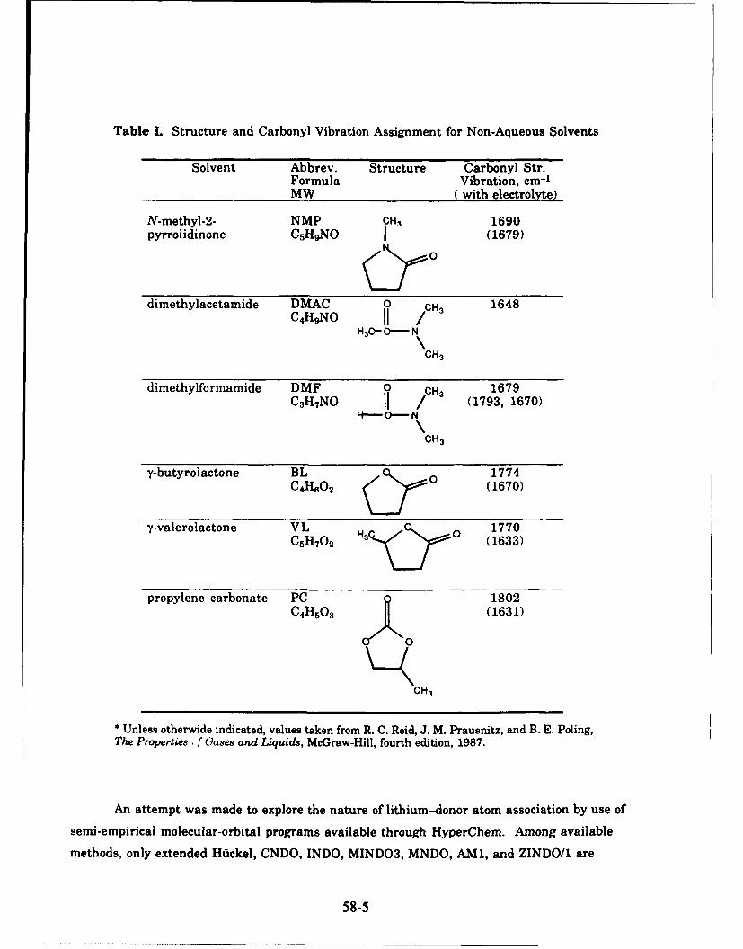
Table L Structure and Carbonyl Vibration Assignment for Non-Aqueous Solvents
Solvent Abbrev. Structure Carbonyl Str.Formula Vibration, cm-'MW (with electrolyte)
N-methyl-2- NMP OH3 1690pyrrolidinone C5H9NO | (1679)
1ro0dimethylacetamide DMAC 0 CH3 1648
H30-O - N
CH3
dimethylformamide DMF 0 CH3 1679C3H7NO jj / (1793, 1670)
H- 0- N
CH3
y-butyrolactone BL 0 1774C 4H6 0 2 (1670)
y-valerolactone VL H3 1770C 5H 70 2 (1633)
propylene carbonate PC 1802
C4H 50 3 (1631)
CH3
* Unless otherwide indicated, values taken from R. C. Reid, J. M. Prausnitz, and B. E. Poling,The Properties, f Gases and Liquids, McGraw-Hill, fourth edition, 1987.
An attempt was made to explore the nature of lithium-donor atom association by use of
semi-empirical molecular-orbital programs available through HyperChem. Among available
methods, only extended Huckel, CNDO, INDO, MINDO3, MNDO, AM1, and ZINDO/1 are
58-5
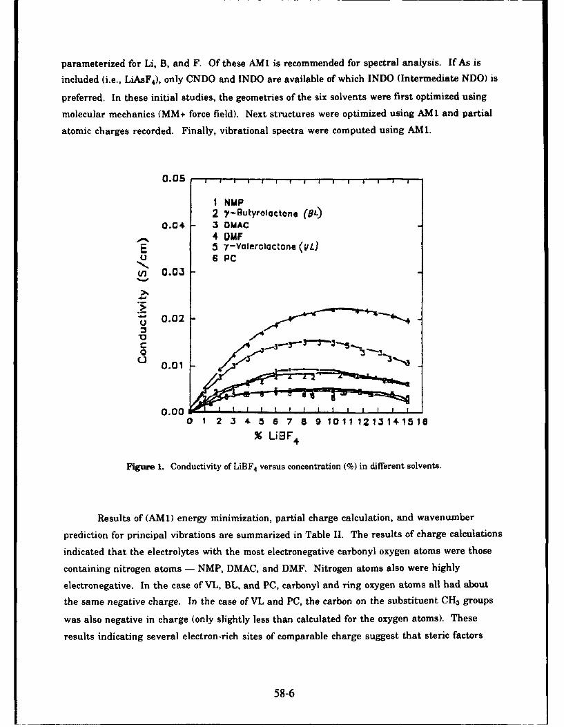
parameterized for Li, B, and F. Of these AMI is recommended for spectral analysis. If As is
included (i.e., LiAsF 4), only CNDO and INDO are available of which INDO (Intermediate NDO) is
preferred. In these initial studies, the geometries of the six solvents were first optimized using
molecular mechanics (MM+ force field). Next structures were optimized using AM1 and partial
atomic charges recorded. Finally, vibrational spectra were computed using AML.
0.05 * , , , ,
I NMP
2 V-Sutyrolactone (8'L)0.04- 3 DMAC
4 DMF"E 5 7Y-Yalerolactone (VL)
9 SPC
cii 0. 03
S0.02
C
L) 0.01
0.000 1 2 3 4 5 6 7 8 9 1011 12 131-1518
% LiBF 4
Figure 1. Conductivity of LiBF 4 versus concentration (%) in different solvents.
Results of (AM1) energy minimization, partial charge calculation, and wavenumber
prediction for principal vibrations are summarized in Table II. The results of charge calculations
indicated that the electrolytes with the most electronegative carbonyl oxygen atoms were those
containing nitrogen atoms - NMP, DMAC, and DMF. Nitrogen atoms also were highly
electronegative. In the case of VL, BL, and PC, carbonyl and ring oxygen atoms all had about
the same negative charge. In the case of VL and PC, the carbon on the substituent CH 3 groups
was also negative in charge (only slightly less than calculated for the oxygen atoms). These
results indicating several electron-rich sites of comparable charge suggest that steric factors
58-6

must also play a significant role in determining how a cation actually interacts with an
electrolyte molecule.
Table H. Results of AM1 Computations
Solvent Optimization Partial Charges on Computed (AMU)Energy Carbonyl Oxygen Frequency (Intensity)Gradient and Other PrincipalCycles AtomsConvergence
NMP 1536.39 carbonyl 0: -0.353 C=0 str: 2048.17 (228.248)0.014 N: -0.351 N: 1637.74 (101.497)155 1515.70 (50.725)No
DMAC 1365.0304 carbonyl 0: -0.373 C=0 str: 1979.04 (179.04)0.005 N: -0.346 C-N str:1620.34 (135.385)35 N: 1574.70 (39.851)Yes
DMF 1085.81 carbonyl 0: -0.361 C=O str: 1995.29 (244.639)0.006 N: -0.357 1589.17 (94.545)35 N: 1582.43 (36.549)Yes 1164.07 (15.219)
BL 1206.8293 carbonyl 0: -0.289 C=O str: 2122.89 (161.483)0.031 ring 0: -0.251 C-0 str: 1487.66 (60.699)148 1346.42 (55.6150No
VL 1486.666 carbonyl 0: -0.293 C=O str: 2121.05 (166.520)0.059 ring 0: -0.251 C-0 ring str: 1468.05 (80.062)223 methyl C: -0.226 1338.32 (36.378)No C-C str: 1290.61 (29.210)
PC 1307.6648 carbonyl 0: -0.277 C=O str: 2162.54 (276.083)0.026 ring 0: -0.244 ring C-O str: 1536.41 (91.737)194 methyl C: -0.229 ring C-0 str: 1272.51 (68.049)No
Results of vibrational analysis are also given in Table II. Principal computed vibrationsare given and assignment of the molecular motion corresponding to each peak is made whereever
possible (HyperChem, Release 3, provides the capability of animating vibrations). Comparison ofexperimental and calculated wavenumbers assigned to the carbonyl stretching vibration is givenin Table III. As the data indicates, the calculated vibrational assignments are 300-400 cm-1
higher than the experimental values. These differences are deemed too large to be able to
interpret calculated vibrational spectra for electrolyte-cation pairs in a meaningful way. Ab
initio methods (e.g., Gaussian 92) should provide better predictions and will be pursued during
the Summer Research Extension Program. It should be noted that spectra calculated by
58-7

Gaussian can be displayed using HyperChem. An attempt will be made to use molecular
dynamics simulation of LiBF 4-electrolyte interactions in a periodic box using HyperChem (or
Quanta/CHARMm) to identify specific Li-electrolyte interactions. Representative complexes will
then be isolated and spectra determined by HyperChem (AM1) and also evaluated using
Gaussian. The spectra obtained in this way for the complexed spectra will then be compared
with that of the pure solvent molecule obtained in the identical fashion
Table HI. Comparison of Experimental and Calculated (AM1)
Carbonyl Vibration Assignments in Wavenumbers (cm- 1 )
Electrolyte Experimental Calculated
NMP 1690 2048DMAC 1648 1979DMF 1679 1995BL 1774 2123VL 1770 2121PC 1802 2163
2. Simulation of Li-Polymer Interaction.
PEO is well-known to assume a 7/2 helical conformation. In order to explore the basis of
the conformational behavior of PEO, an oligomer containing 8 repeating units HO(CH 20)s-H
was constructed using Hyperchem. The structure was optimized using molecular mechanics
(AMBER force field) and with the use of AML. The result was an extended zig-zag chain with
oxygen atoms alternating along the chain as shown in Figure 2. Bond lengths and angles are
given in Table IV. The total energy calculated by AM1 (134 orbitals) was -1.2459 x 10⁵ kcal
mol-I (Grad=1.041 kcal mol-i A-i). Partial charges were -0.29 for oxygen, -0.021 for carbons,
and +0.082 for H (these were essentially unchanged when optimization was continued to 32
computational cycles for which Grad = 0.073).
58-8

Figure 2. Extended chain structure of PEO8 obtained by AM1 geometry optimization.
The extended chain conformation obtained by geometry optimization differs from the 7/2
helix suggested from X-ray crystallographic data appearing in the literature. In order to
compare the energies of the extended chain and helical chain conformations, a helix was imposed
on the PEO structure by constraining the torsional angles as follows: C-C-C , trans (1800); C-O-C-C, trans (1800); and O-C-C-0, gauche (-1800). A representation of the resulting helical
conformation is given in Figure 3. The total energy calculated by AM1 (134 orbitals) was -1.2456x 10⁵ kcal mol-I (Grad=15.824 kcal mol-I A-') which is very close to that of the extended chain.
Partial atomic charges were approximately -0.25 for oxygens (-0.33 for the terminal hydroxyl
oxygens), -0.02 for carbon atoms, and +0.07 for hydrogen. The charge on oxygen in the helical
conformation is slightly less negative and that on the hydrogen atoms slightly less positive than
calculated for the extended chain structure (the charge on the carbon atoms were essentially
unchanged). Interestingly, the dipole momemt calculated for helical PEO was significantly larger(2.809 D) for the helical conformation than for the extended chain (1.719 D).
58-9

Table IV. Structural Parameters Obtained for PEO Oligomer from
AMI Optimization of Geometry
C-O bond length 1.426C-C bond length 1.526 AC-H bond length 1.121 AC-O-C bond angle 111.90C-C-O bond angle 105.50C-C-O-C torsional angle 180C-O-C-C torsional angle 1800O-C-C-O torsional angle 1800
Figure 3. Helical conformation of PEO8 obtained by constraining torsional angles.
3. Simulation of Macromolecular Ion-Transport Tunnels.
An objective for the Electrochemistry Laboratory at Wright-Patterson AFB is the
development of new electrolytes capable of high conductivity at low temperatures. One approach
being evaluated is the development of a lithium ion-conducting polymer-electrolyte based on
ionically conducting polymer tubes formed by stacking macrocyclic rings. The hope is that a
suitable geometry can be defined such that the lithium ion experiences a constant solvation-
coordination sphere throughout the molecular tube. In this manner, ionic conduction would occur
by means of ion "hopping" that could result in substantially higher conductivity compared to ion
conduction resulting from molecular motion.
58-10
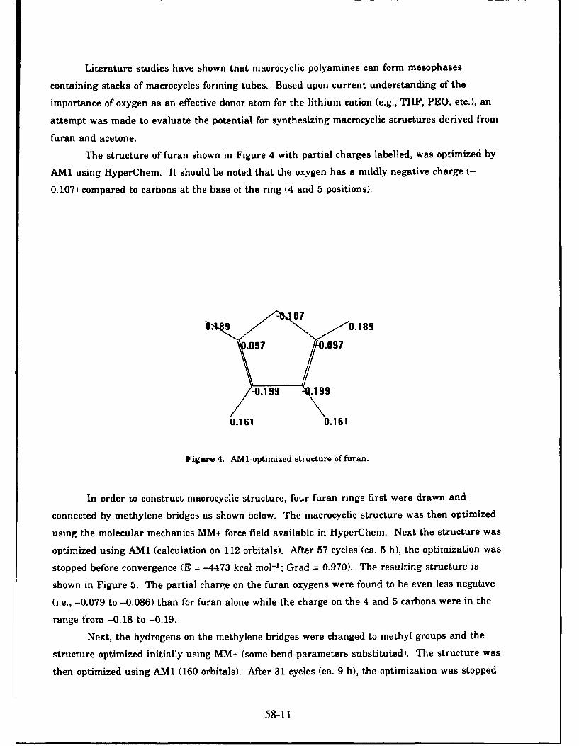
Literature studies have shown that macrocyclic polyamines can form mesophases
containing stacks of macrocycles forming tubes. Based upon current understanding of the
importance of oxygen as an effective donor atom for the lithium cation (e.g., THF, PEO, etc.), an
attempt was made to evaluate the potential for synthesizing macrocyclic structures derived from
furan and acetone.
The structure of furan shown in Figure 4 with partial charges labelled, was optimized by
AM1 using HyperChem. It should be noted that the oxygen has a mildly negative charge (-
0.107) compared to carbons at the base of the ring (4 and 5 positions).
.18
/4.199 -•t199
0.161 0.161
Figure 4. AM1-optimized structure of furan.
In order to construct macrocyclic structure, four furan rings first were drawn and
connected by methylene bridges as shown below. The macrocyclic structure was then optimized
using the molecular mechanics MM+ force field available in HyperChem. Next the structure was
optimized using AM1 (calculation on 112 orbitals). After 57 cycles (ca. 5 h), the optimization was
stopped before convergence (E = -4473 kcal mol-1; Grad = 0.970). The resulting structure is
shown in Figure 5. The partial charge on the furan oxygens were found to be even less negative
(i.e., -0.079 to -0.086) than for furan alone while the charge on the 4 and 5 carbons were in the
range from -0.18 to -0.19.
Next, the hydrogens on the methylene bridges were changed to methyl groups and the
structure optimized initially using MM+ (some bend parameters substituted). The structure was
then optimized using AM1 (160 orbitals). After 31 cycles (ca. 9 h), the optimization was stopped
58-11

(E = -6686.36 kcal mol-I and Grad = 1.470) and then single-point calculations were made. The
structure shown in Figure 6 indicates that two opposite furan rings are pointed upward and two
are pointed downwide. Partial charges calculated for the furan oxygens are comparable (ca.
-0.08) to the previous case; however, the partial charges of the methylene groups are reasonably
electronegative (i.e., -0.2).
Figure 5. Macrocycle with methylene bridges (MACRO1).
Figure 6. Macrocycle with dimethyl bridges (MACRO2).
58-12

Next, additional resonance structure is introduced through the incorporation of carbon
double bonds on the bridge groups. This gave a macrocycle where the rings fell within a single
plane upon initial structure builiding. The structure was then optimized using AMI (128
orbitals). After 37 cycles (ca. 4 h), the optimization was terminated (E = -5034 and Grad = 2.630)
and single-point calculations were made. The structure was nearly totally planar with all oxygen
atoms pointing inward as shown in the Figure 7. Three-dimensional models indicate that two
opposite furan rings are pointing slightly downward and two are pointing slightly upward.
Values calculated for partial charges, as shown in Figure 8, indicate a more extensive resonance
of the ring structure giving only very low negative charge (ca. -0.04) to the furan oxygens.
Distances between opposite furan oxygens were 4.2-4.3 A.
Figure 7. AM1 optimized macrocycle with unsaturated bridges.
58-13

0.19
0. 0.
-0.I W .19
Figure 8. Partial charges obtained from single-point calculations of AMi-optimized macrocycle withunsaturated bridges.
Next, a pre-reactive substituent group
0
li- .H2 0--- 00 1H3
was attached to each furan ring of the AMl-optimized dimethyl bridged macrocyclic (MACRO2)
and the overall structure minimized using MM+ (default parameters used for bends). Ater 1072
cycles, the optimization was stopped at E = 34.827 and Grad = 0.096. The structure (MACRO4)
was almost a cage as shown in Figure 9.
58-14
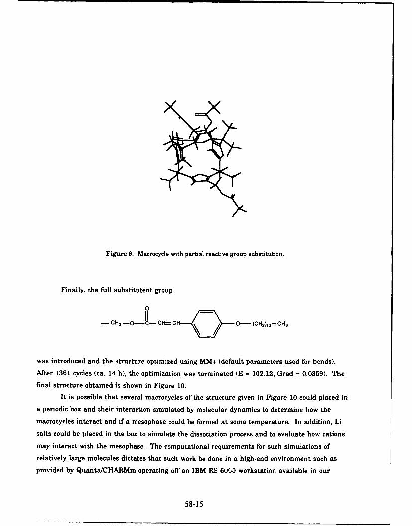
Figure 9. Macrocycle with partial reactive group substitution.
Finally, the full substitutent group
0
-CH 2 - CI=CH / O- (CH 2)13 -CH 3
was introduced and the structure optimized using MM+ (default parameters used for bends).
After 1361 cycles (ca. 14 h), the optimization was terminated (E = 102.12; Grad = 0.0359). The
final structure obtained is shown in Figure 10.
It is possible that several macrocycles of the structure given in Figure 10 could placed in
a periodic box and their interaction simulated by molecular dynamics to determine how the
macrocycles interact and if a mesophase could be formed at some temperature. In addition, Li
salts could be placed in the box to simulate the dissociation process and to evaluate how cations
may interact with the mesophase. The computational requirements for such simulations of
relatively large molecules dictates that such work be done in a high-end environment such as
provided by Quanta/CHARMm operating off an IBM RS 60W0 workstation available in our
58-15
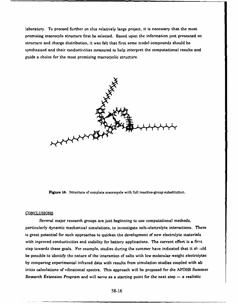
laboratory. To proceed further on this relatively large project, it is necessary that the most
promising macrocyle structure first be selected. Based upon the information just presented on
structure and charge distribution, it was felt that first some model compounds should be
synthesized and their conductivities measured to help interpret the computational results and
guide a choice for the most promising macrocyclic structure.
Figure 10. Structure of complete macrocycle with full reactive-group substitution.
CONCLUSIONS
Several major research groups are just beginning to use computational methods,
particularly dynamic mechanical simulations, to investigate salt-electrolyte interactions. There
is great potential for such approaches to quicken the development of new electrolyte materials
with inproved conductivities and stability for battery applications. The current effort is a first
step towards these goals. For example, studies during the summer have indicated that it shuld
be possible to identify the nature of the interaction of salts with low molecular-weight electrolytes
by comparing experimental infrared data with results from simulation studies coupled with ab
initio calculations of vibrational spectra. This approach will be proposed for the AFOSR Summer
Research Extension Propram and will serve as a starting point for the next step - a realistic
58-16

simulation of salt-polymer interactions. Initial studies of PEO8 indicate the importance of using
the proper polymer conformational state in such work. Finally, the summer effort has shown that
computer modeling can be a useful aid in evaluating different approaches for synthesizing new
macrocyles for possible electrolyte applications.
ACKNOWLEDGMENT
This Research Associate wishes to express his gratitude to Dr. Lawrence G. Scalon, Jr.,
and Dr. Woitek Kravitz for their very helpful advice and guidance during the summer and for
providing this opportunity to learn a new area of research and develop my computational skills
outside the demanding distractions of everyday academic life.
58-17

COMPARISON OF HYDRAULIC AND THERMAL PERFORMANCE
OF PAO AND COOLANOL 25R LIQUID COOLANTS
Afshin J. Ghajar
Professor
School of Mechanical and Aerospace Engineering
Oklahoma State University
Stillwater, OK 74078
Final Report for:
Summer Faculty Research Program
Wright Laboratory
Sponsored by:
Air Force Office of Scientific Research
Bolling Air Force Base, Washington, D.C.
August 1993
59-1
COMPARISON OF HYDRAULIC AND THERMAL PERFORMANCEOF PAO AND COOLANOL 25R LIQUID COOLANTS
Afshin J. GhajarProfessor
School of Mechanical and Aerospace EngineeringOklahoma State University
Abstract
A general method for the comparison of hydraulic and thermal performance
of different liquid coolants is offered. Thermophysical property expressions
for the variation of density, specific heat, thermal conductivity, and
kinematic viscosity with temperature for PAO and Coolanol 25R were developed.
The range of temperature for this study was from -54 to 135"C. Based on the
results, the hydraulic performance of Coolanol 25R is much better than PAO at
low temperatures (below 0"C) and laminar flow regime. In the turbulent
region, PAO hydraulically outperforms Coolanol 25R over the entire temperature
range. The thermal performance of PAO at temperatures below 61'C and in the
laminar flow region, is slightly better than Coolanol 25R. In the low
temperature turbulent region, Coolanol 25R thermally outperforms PAO. At
other temperatures, the performance of the two liquid coolants are reasonably
close and fairly independent of the flow regime.
59-2

COMPARISON OF HYDRAULIC AND THERMAL PERFORMANCE
OF PAO AND COOLANOL 25R LIQUID COOLANTS
Afshin J. Ghajar
Introduction
Silicate-ester-based fluids (e.g. Coolanol 25R) are widely used as
dielectric heat transfer fluids in the Air Force and the Navy airborne radar
and missile systems. These fluids have caused significant and sometimes
catastrophic problems due to their hygroscopic nature and subsequent formation
of flammable alcohols and silica gel. The alcohol by-product lowers the fluid
flashpoint, increasing the risk of aircraft fires. The gelatinous precipitate
called the "black plague", deposits on transmitter surfaces and components,
causing avionics equipment to malfunction.
In order to solve the problems associated with silicate-ester-based
fluids, the Naval Air Development Center and the Air Force Materials
Directorate investigated the possibility of direct replacement of silicate-
ester-based fluids with hydrogenated polyalphaolefin-based fluids. Their
studies concluded that polyalphaolefin (PAO) fluids are chemically more stable
(they do not hydrolyze to form either silica gel or alcohol by-products), less
costly, offer equal or improved dielectric characteristics, and meet or exceed
military requirements for a dielectric coolant [1-4].
Due to the inherent desirable properties of PAO, their ready
availability, and their relatively low cost (about one-fifth of the cost of
current silicate-ester-based fluids), the Air Force and the Navy have both
replaced the current heat transfer fluid in the avionics system with PAO for
some selected aircrafts. Other aircrafts may soon follow. Although,
replacement of silicate-ester-based fluids with PAO fluid reduces the risk of
aircraft fire and eliminates the coolant fluid contamination problem which
results in "black plague", the overall performance of the avionics liquid
cooling system with PAO in comparison to silicate ester fluids over a wide
temperature range has not been fully studied. Limited unpublished studies
have been conducted on the performance of specific aircraft radar transmitters
with PAO [2,3].
The objective of this study was to compare the hydraulic and thermal
performance of PAO and silicate ester fluids in a temperature range (-54 to
59-3

135"C) applicable to avionics equipment. Both laminar and turbulent flow
regimes were considered. In order for the analysis to be general, variation
of dimensionless system parameters with temperature are presented. In
addition, as part of this study, equations were developed for the variation of
thermophysical properties of Coolanol 25R and PAO with temperature.
THERMOPHYSICAL PROPERTIES EOUATIONS
Knowledge of thermophysical properties of the Coolanol 25R and PAO
fluids as a function of fluid temperature was required for hydraulic and
thermal performance analysis. Thermophysical property data for Coolanol 25R
and PAO (Brayco Micronic 889) were obtained from technical data sheets
provided by Chevron [5] and Castrol [6], respectively. The density (p),
specific heat (cp), and thermal conductivity (k) data were easily curve-fitted
in the form of a polynomial in temperature using a least squares curve-fitting
program. The degree of the fitted polynomial, in some cases, varied between
the two fluids for the same thermophysical property. In order to avoid
listing several different equations, the general form of the curve-fitted
equation with the highest obtained degree of polynomial is presented in the
form
[PROPERTY] = A + BT + CT 2 + DT 3 + ET 4 + FT 5 (I)
In Eq. (1), the term "PROPERTY" can be either density in kg/m3 , specific heat
in kJ/kg-K or thermal conductivity in W/m-K, and the temperature (T) is in K.
The curve-fitted constants A to F to be used in Eq. (1) for Coolanol 25R
(C25R) and PAO are tabulated in Table 1. The curve-fitted equations for p, cp,
and k predict the PAO and Coolanol 25R data with a maximum deviation of less
than ±0.5%.
For variation of kinematic viscosity with temperature, the viscosity-
temperature relationship suggested for petroleum oils or liquid hydrocarbons
[7] was curve-fitted to the Coolanol 25R and PAO data. The equation is of the
form
D = 10 (10A/TB) - C (2)
In Eq. (2), the kinematic viscosity (v) is in m2 /s and the temperature (T) is
in K. The curve-fitted constants A, B, and C to be used in Eq. (2) for
Coolanol 25R (C25R) and PAO are also tabulated in Table 1. The curve-fitted
equation for v predicts the thirteen Coolanol 25R data points with a maximum
deviation of +5.5% and an average absolute deviation of 1.9%. For the
59-4

thirteen PAO data points the maximum deviation was +3.4% with an average
absolute deviation of 1.3%.
Table 1. Curve-Fitted Constants for Density, Specific Heat, ThermalConductivity, and Kinematic Viscosity Equations.
PRCPERTY FLUID A B C D E F
C25R 1.13 x 10³ -0.784
PPAO 1.36 x 10³ -4.56 0.0157 -0.280 x 10⁻⁴ 0.174 x 10⁻⁷
C25R 0.492 4.49 x 10⁻³cp PAO 1.022 3.77 x 10⁻³
C25R 0.453 -4.64 x 10⁻³ 0.275 x 10⁻⁴ -0.809 x 10⁻⁷ 0.117 x 10⁻⁹ -0.667 x 10" 3k
PAO 0.154 -5.88 x 10⁻⁵
C25R 8.36 3.408 0.802
PAO 9.67 3.923 0.700
The variation of p, cp, k, and u with temperature for Coolanol 25R (C25R)
and PAO over the temperature range from -54 to 135"C are compared in Figures 1
to 4, respectively. Another thermophysical property that plays an important
role in the hydraulic and thermal performance of coolants is absolute
viscosity (p). The variation of g with temperature for the two fluids is
shown in Figure 5. The values of g were determined from the product of
density and kinematic viscosity values.
The expressions zid the constants for the thermophysical properties
presented in this section were also programmed. The interactive computer
program produces thermophysical properties for Coolanol 25R or PAO at any
temperature in the range from -54 to 135"C, in either SI or English units.
Single or multi-point calculations caii be performed. The tabulated results
can be viewed on the screen and/or stored into a specified data file.
HEAT TRANSFER PARAMETER
From a heat transfer viewpoint, coolants are rated by first considering
the applicable heat transfer correlating equation. Considering a problem of
heat transfer in forced convection to a fluid in a duct or channel, the
following general form of heat transfer correlation is applicable59-5
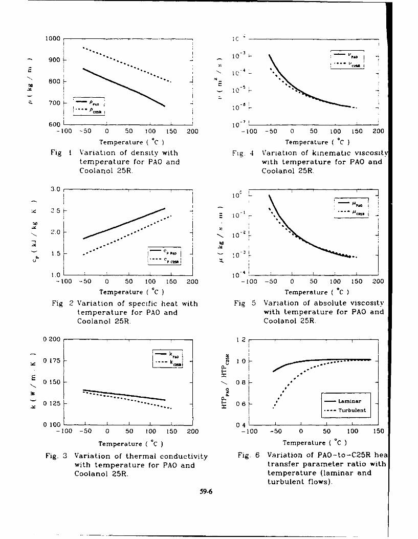
1000 I
9 00 torh
E o I t
800" -4
10I. i -7 00 P
600 10-
-100 -50 0 50 100 150 200 -100 -50 0 50 100 150 200
Temperature ( 0C ) Temperature ( 0CFig I Variation of density with Fig. 4 Variation of kinematic viscosity
temperature for PAO and with temperature for PAO andCoolanol 25R. Coolanol 25R.
300' A
o I
-t N• O--10
15 C PPAO i 0 3 1-4I____....________________________
1.0 t o . 4 10-4 !: . .
-100 -50 0 50 100 150 200 -100 -50 0 50 100 150 200
Temperature ( "C ) Temperature ( 0C )
Fig 2 Variation of specific heat with Fig. 5 Variation of absolute viscositytemperature for PAO and with temperature for PAO and
Coolanol 25R. Coolanol 25R.
0200 1 1 2r
0175 k:]. N 1 0
E 0 150 08
0a.*
-I02 .... ...... I 6 -.. urlen0 100 I I 04
-100 -50 0 50 100 150 200 -100 -50 0 50 100 150
Temperature ( 0C ) Temperature ( 0C )
Fig. 3 Variation of thermal conductivity Fig. 6 Variation of PAO-to-C25R heawith temperature for PAO and transfer parameter ratio withCoolanol 25R. temperature (laminar and
turbulent flows).59-6
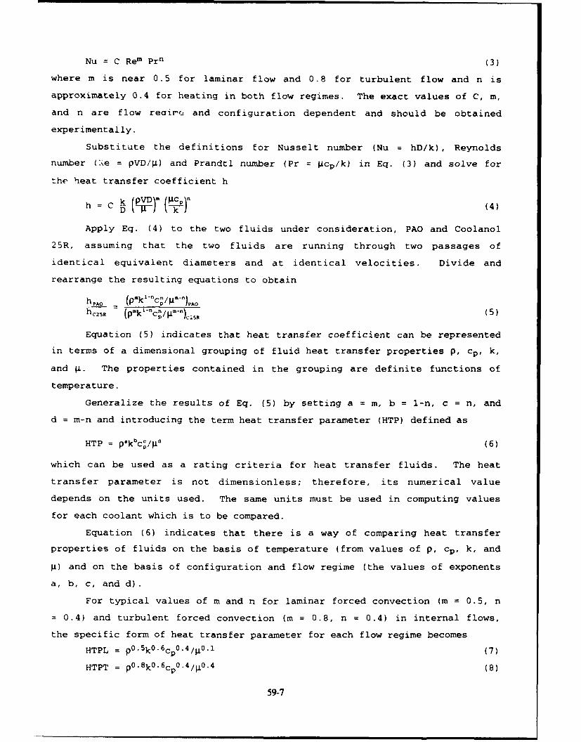
Nu = C Rem Prn (3)
where m is near 0.5 for laminar flow and 0.8 for turbulent flow and n is
approximately 0.4 for heating in both flow regimes. The exact values of C, m,
and n are flow reairu" and configuration dependent and should be obtained
experimentally.
Substitute the definitions for Nusselt number (Nu = hD/k), Reynolds
number (Ce = pVD/L) and Prandtl number (Pr = gcp/k) in Eq. (3) and solve for
the heat transfer coefficient h
h=Ch- D(17)o (,!E.)n (4)
Apply Eq. (4) to the two fluids under consideration, PAO and Coolanol
25R, assuming that the two fluids are running through two passages of
identical equivalent diameters and at identical velocities. Divide and
rearrange the resulting equations to obtainm I-n n/pm-n)"
hpAo - (pmk )j )hcz5 R kic-n/n m-n) (5)
(C25c (pok PEquation (5) indicates that heat transfer coefficient can be represented
in terms of a dimensional grouping of fluid heat transfer properties p, cp, k,
and g. The properties contained in the grouping are definite functions of
temperature.
Generalize the results of Eq. (5) by setting a = m, b = 1-n, c = n, and
d = m-n and introducing the term heat transfer parameter (HTP) defined as
HTP = pakbcc /gd (6)
which can be used as a rating criteria for heat transfer fluids. The heat
transfer parameter is not dimensionless; therefore, its numerical value
depends on the units used. The same units must be used in computing values
for each coolant which is to be compared.
Equation (6) indicates that there is a way of comparing heat transfer
properties of fluids on the basis of temperature (from values of p, cp, k, and
g) and on the basis of configuration and flow regime (the values of exponents
a, b, c, and d).
For typical values of m and n for laminar forced convection (m = 0.5, n
0.4) and turbulent forced convection (m = 0.8, n = 0.4) in internal flows,
the specific form of heat transfer parameter for each flow regime becomes
HTPL = p°- 5 k°. 6cp°. 4 /g°.- (7)
HTPT = p0 .8 k0 -6Cp0 .4 /g0. 4 (8)
59-7
where HTPL and HTPT designate the laminar and turbulent heat transfer
parameters, respectively.
Apply Eq. (7) or (8) to Eq. (5) to obtain an expression for the ratio of
PAO-to-Coolanol 25R heat transfer coefficients in terms of the heat transfer
parameter. Figure 6 shows the variation of PAO-to-C25R heat transfer
parameter ratio with temperature for laminar and turbulent flow regimes. The
figure indicates that there could be a substantial difference between the heat
transfer properties of the two fluids. This :'ifference strongly depends on
the coolant flow regime and the coolant operating temperature. In laminar
flow regime (see the solid line in Fig. 6), at the lowest coolant temperature
(-54"C), the heat transfer parameter for PAO is about 11% lower than that of
Coolanol 25R, and this difference quickly diminishes to about 2% at -14"C. At
temperatures above -14'C, there is virtually no difference in the heat
transfer properties of the two fluids. However, in turbulent flow, the
differences are much larger and are sustained over a larger temperature range.
Referring to the dashed line in Figure 6, at -54"C the heat transfer parameter
for PAO is about 78% lower than that of Coolanol 25R. This difference slowly
reduces to about 21% at -14"C and to about 2% at 56"C. Beyond this
temperature, the two fluids behave the same way.
Overall, from a heat transfer view point, Coolanol 25R outperforms PAO
in the low temperature region in both flow regimes. The difference is much
more substantial for turbulent flow in the temperature range from -54"C to
about 6"C. Therefore, at these low temperatures, in order for the heat
transfer characteristics of the systems operating with PAO to be fairly
comparable with the Coolanol 25R systems, operation in the laminar flow regime
is recommended. The type of analysis presented here indicates how it can
definitely be established which fluid has the better heat transfer properties.
HYDRAULIC PERFORMANCE
Comparison of hydraulic performance of PAO and Coolanol 25R is based on
the relationship between pressure drop and flow rate. The Moody diagram [8]
establishes the proper normalized dimensionless pressure drop parameter [f =
AP/(L/D)(I/2pV2 )] and flow parameter (Re = pVD/I) for a rounO pipe with a fixed
relative roughness in the form
f = 0 ,I (Re) (9)
where 0i is a function to be determined experimentally or analytically.
Therefore, when the data is plotted as f versus Re, usually a log-log plot,
59-8
the data points fall on a single curve, for a constant value of a relative
roughness.
The major difficulty in application of Eq. (9) to an avionics system is
associated with the proper evaluation of diameter (D) and fluid velocity (V)
in the definitions of f and Re. The coolant flow loop for an avionics system
(e.g. radar transmitter) is very different than a long, straight, round pipe.
In the coolant flow loop there are numerous bends, sudden expansions and
contractions, change of flow areas, non-circular flow passages, and other
local obstructions, the combined effect of which results in the overall
pressure drop of the system. Therefore, the diameter (D), appearing in the
definitions of f and Re must represent these effects. However, for a given
system each of these local effective diameters is a constant, and consequently
their combined influence can be included as a constant in the function 01 of
Eq. (9). The fluid velocity (V), appearing in the definitions of f and Re
must also be representative of the various local velocities within the system,
due to the existence of numerous different flow areas, and hence different
velocities in the system. However, the velocity at any given point in the
sys-em differs from the volume flow rate (Q) only by the local flow area which
is considered constant. Therefore, V can be replaced by Q, and the local
invariant flow areas can be included as constants in the function 01 of Eq.
(9).
Based on the above discussion, the definitions of f and Re and Eq. (9)
can be rearranged in the form
P = 02 (F) (10)
where P = AP/pQ2 and F = Q/v are the new normalized dimensional pressure drop
and flow parameters, respectively. It should be realized that these
parameters are not dimensionless and Eq. (10) is a dimensional equation, and
that the function 02 (which must be determined experimentally) is different for
each system. This is in sharp contrast to the function 01 in Eq. (9) for a
circular pipe flow, where the same function applies to all round pipes with a
fixed relative roughness.
A simple form of the function 02 in Eq. (10) can be determined for low
and high values of Reynolds number by inspection of Moody diagram [8]. For
low Re values (laminar flow), the f versus Re is a straight line with slope of
-1. For high Re values (complete turbulence), f versus Re for a given
relative roughness is a straight line with a slope of zero.
59-9
The new dimensional parameters P and F differ from the Moody
dimensionless parameters f and Re, by only an unknown constant at each
location in ae system. Therefore, the following equation should represent
the functic. ,I form (02) that exists between P and F for low and high Reynolds
numbers
B (11)P = A + F ii
where A and B are experimentally determined constants for a given system.
A plot of Eq. (11) for a hypothetical situation is shown as Figure 7.
This figure is a log-log plot of pressure drop parameter (P) and flow
parameter (F). The plot exhibits a slope of -1 at low values of F (P = B/F)
and approaches a slope of zero at high values of F (P - A). These terminal
slopes are indicative of fully laminar flow at low values of F and fully
turbulent flow at high values of F and are comparable with the Moody diagram.
It should be realized that the constants A and B in Eq. (11) are unique for a
given system but are independent of the type of fluid used in the system.
This allows for generalization of the hydraulic performance of the system for
the two limiting cases of Eq. (11). These limiting cases are referred to as
the fully laminar and fully turbulent and will be discussed next.
Fully Laminar Case: for this case, Eq. (11) can be approximated by P =
B/F. Using the definitions of P and F and solving for AP results in
AP = Bgo (12)
Eq. (12) implies that the pressure drop and volume flow rate depend strongly
on the absolute viscosity of the heat transfer fluid. Apply Eq. (12) to the
two fluids under consideration, PAO and Coolanol 25R, assuming the two fluids
are running through two identical systems at identical coolant flow rates.
Divide the resulting equations to obtain
APpAO = -P-A (13)APC25 R 9C25R
An equation similar to Eq. (13) can be developed for the volume flow rate
ratio of the two fluids, assuming identical systems at identical pressure
drops. The resulting equation is
QPAO- = 1C251t( 4
QC25R PvAo (14)
The variations of PAO-to-C25R pressure drop and volume flow rate ratios
with coolant temperature are shown in Figure 8, by the solid and broken lines,
respectively. The figure indicates that the ratios vary dramatically in the
59-10

temperature range from -54 to 26"C. At these low temperatures the pressure
drop ratio varies from about 1 at 26'C to about 4.4 at -54"C. This four fold
increase in the pressure drop is due to the much higher absolute viscosity of
PAO at these low temperatures (see Fig. 5). At temperatures warmer than 26"C,
the pressure drop variation with temperature is relatively small and
approaches unity at 46"C. At temperatures greater than 46"C, the pressure
drop ratio drops below unity, indicating that the system with Coolanol 25R as
the working fluid, experiences higher pressure drop than the system with PAO
at identical operating conditions. The pressure drop difference increases
with temperature, and at the highest temperature of 135"C, reaches a value of
about 16%.
The variation of volume flow rate ratio with coolant temperature shown
by the broken line in Figure 8, demonstrates a trend similar but opposite to
the pressure drop ratio. At low temperatures, the volume flow rate of PAO is
much smaller than that of Coolanol 25R for the same identical operating
conditions and pressure drop. This difference decreases with increasing
temperature and the ratio approaches unity around 46"C. At temperatures
greater than 46"C, the volume flow rate ratio goes above unity, indicating
that for the same operating conditions, the Coolanol 25R volume flow rate is
lower in comparison to PAO.
The observations made about the variation of PAO-to-C25R pressure drop
and volume flow rate ratios in the laminar flow region, should be put in the
context of the overall system operation. The higher pressure drop associated
with PAO at low temperatures (<26"C) means that when replacing Coolanol 25R
with PAO, the system pump must be capable of handling the additional losses at
these low temperatures. The low volume flow rate of PAO at low temperatures
may not be adequate to satisfy the cooling requirements of the electronic
equipments. However, replacement of Coolanol 25R with PAO, from the stand
point of hydraulic performance, appears to be advantageous when operating in
the laminar flow regime at temperatures above 46"C.
Fully Turbulent Case: for this case, Eq. (11) can be approximated by P
= A. Using the definitions of P and F and solving for AP results in
Ap = ApQ2 (15)
Equation (15) implies that the pressure drop and volume flow rate depend
strongly on the density of the heat transfer fluid. Apply Eq. (15) to the two
fluids under consideration and follow the same identical assumptions and
59-11
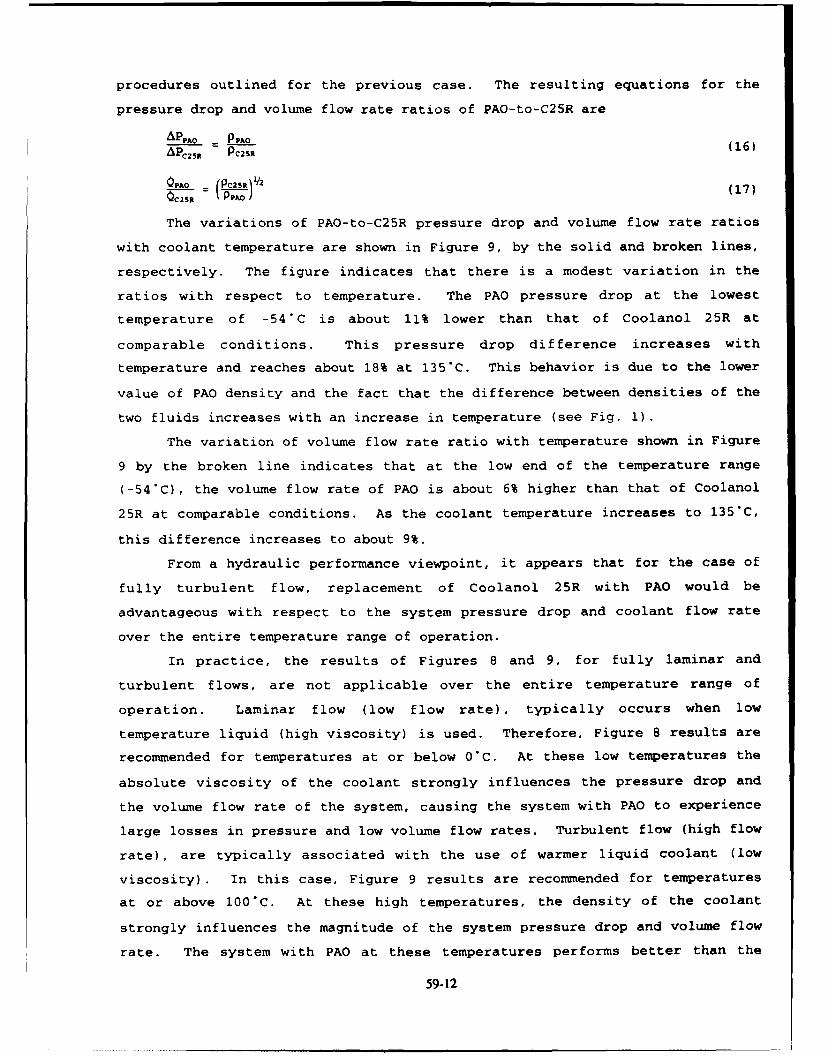
procedures outlined for the previous case. The resulting equations for the
pressure drop and volume flow rate ratios of PAO-to-C25R are
APpi 0 PPAO (16)AyPZS - PC25R
O0Ao (Pc2s&t½ (17)OC25R 'PPAO
The variations of PAO-to-C25R pressure drop and volume flow rate ratios
with coolant temperature are shown in Figure 9, by the solid and broken lines,
respectively. The figure indicates that there is a modest variation in the
ratios with respect to temperature. The PAO pressure drop at the lowest
temperature of -54"C is about 11% lower than that of Coolanol 25R at
comparable conditions. This pressure drop difference increases with
temperature and reaches about 18% at 135"C. This behavior is due to the lower
value of PAO density and the fact that the difference between densities of the
two fluids increases with an increase in temperature (see Fig. 1).
The variation of volume flow rate ratio with temperature shown in Figure
9 by the broken line indicates that at the low end of the temperature range
(-54"C), the volume flow rate of PAO is about 6% higher than that of Coolanol
25R at comparable conditions. As the coolant temperature increases to 135'C,
this difference increases to about 9%.
From a hydraulic performance viewpoint, it appears that for the case of
fully turbulent flow, replacement of Coolanol 25R with PAO would be
advantageous with respect to the system pressure drop and coolant flow rate
over the entire temperature range of operation.
In practice, the results of Figures 8 and 9, for fully laminar and
turbulent flows, are not applicable over the entire temperature range of
operation. Laminar flow (low flow rate), typically occurs when low
temperature liquid (high viscosity) is used. Therefore, Figure 8 results are
recommended for temperatures at or below 0"C. At these low temperatures the
absolute viscosity of the coolant strongly influences the pressure drop and
the volume flow rate of the system, causing the system with PAO to experience
large losses in pressure and low volume flow rates. Turbulent flow (high flow
rate), are typically associated with the use of warmer liquid coolant (low
viscosity). In this case, Figure 9 results are recommended for temperatures
at or above 100"C. At these high temperatures, the density of the coolant
strongly influences the magnitude of the system pressure drop and volume flow
rate. The system with PAO at these temperatures performs better than the
59-12

Coolanol 25R system. In the intermediate temperature range from 0 to 100"C,
the flow might not be either fully laminar or fully turbulent and the use of
Figures 8 or 9 might be questionable. In this temperature range, the pressure
drop and the volume flow rate depend on both the density and the absolute
viscosity of the coolant. However, the viscosity difference between PAO and
Coolanol 25R is less extreme (see Fig. 5), and the lower density of PAO (see
Fig. 1) has more influence on the PAO-to-C25R pressure drop and volume flow
rate ratios, tending to counteract the influence of higher absolute ,iscosity.
The end result would be ratios close to unity. Therefore these
temperatures the hydraulic performance of the PAO and Coolanol 3 •ystems
should be very comparable.
THERMAL PERFORMANCE
One of the major objectives in the thermal analysis of an electronic ox
(e.g. radar transmitter), is the determination of the component hot spot
surface temperature. This temperature is determined by adding all of the
temperature rises along the heat flow path to the inlet temperature of the
coolant. For the thermal performance analysis, assuming identical systems
with the exception of the liquid coolant, only the liquid coolant
contributions to the component surface temperature were considered.
Temperature rises across the interface or in solids were ignored in this
analysis. The liquid coolant contributes in two ways to the component surface
temperature: (1) temperature rise due to the heat input from the electronics
to the coolant as it flows through the electronic box, ATC; and (2)
temperature rise due to the thermal resistance across the liquid coolant
convection-film from the surface of the component to the coolant, ATF. The
basic forced liquid flow relationships needed for determination of these
temperature rises will be presented next [9, 10].
The temperature rise in a liquid cooled system can be determined from
ATC = 4/(Pcp)Q (18)
where ATC is the coolant temperature rise, 4 is the power dissipation, Q is
the volume flow rate of coolant, and (pcp) is the heat capacity of the coolant.
In a forced liquid system, a convection-film develops and clings to the
heat transfer surface and restricts the flow of heat from the electronic
components to the liquid coolant. The temperature rise across the forced
convection film (ATF) then becomes:
ATF = '1/hA (19)
59-13

103
S 102
C.-
10' -I
10100to0.4 103 1 2 1O- 1 0 10 ; 02
F
Fig. 7 Funcional form between pressuredrop parameter and flow parameterfor a hypothetical situation.
4 -
Temperature ( °C )
Fig. 8 Variation of PAO-to-C25R pressure
drop or volume flow rate ratios withtemperature (fully laminar case).
0
ca 1.0 PA 2
CL U 4PAO' 4M
0
CL 09
-100 -50 0 50 100 150
Temperature ( 0C )
Fig. 9 Variation of PAO-to-C25R pressure
drop or volume flow rate ratios with
temperature (fully turbulent case).
59-14

where q is the power dissipation, h is the forced convection heat transfer
coefficient, and A is the component surface area.
The influence of different coolants (PAO and Coolanol 25R) and flow
regimes (laminar and turbulent) on the temperature rises obtained from Eqs.
(18) and (19) will be discussed next.
Liauid Coolant Temperature Rise: Apply Eq. (18) to the two fluids under
consideration, assuming two identical systems at identical power dissipations
and coolant flow rates. Divide the resulting equations to obtain
ATCPAO - (pcP) C25R
ATCC25 R (pcP) PAO (20)
An equation identical to Eq. (20) can be developed for volume flow rate ratio
of the two fluids, assuming identical systems at identical power dissipation
and coolant temperature rises. The resulting equation is
QPAO = (pcP) C25R
QC25 R (pcp) PAo (21)
Comparison of Eqs. (20) and (21) shows that the PAO-to-C25R coolant
temperature rise and volume flow rate ratios are directly proportional to the
C25R-to-PAO heat capacity ratio. The variation of ratios given in Eqs. (20)
and (21) with coolant temperature are shown in Figure 10. The results of this
figure can be better understood by examining Figure 11 which shows the
variation of heat capacities with temperature for the two fluids. The figures
indicate that due to the higher heat capacity of PAO at temperatures below
61"C, the coolant temperature rise is lower than that of Coolanol 25R at the
same coolant flow rate. The maximum difference is about 12% at the lowest
temperature of -54"C. Therefore, for temperatures below 61"C, the
contribution from coolant temperature rise to the component surface
temperature would be smaller using PAO as opposed to Coolanol 25R, assuming
the same coolant flow rates. For coolant temperatures above 61"C, the reverse
is true. The Coolanol 25R temperature rise is lower than that of PAO. The
difference reaches a maximum of about 7% at 135"C.
The results presented in Figure 10 can also be interpreted as the
variation of PAO-to-C25R volume flow rate ratio with temperature for the same
coolant temperature rise. As indicated, at the lowest temperature of -54"C,
in order to have the same coolant temperature rise for the two fluids, the
volume flow rate of PAO should be about 1.12 times greater than that of
Coolanol 25R. This is in sharp contrast with the hydraulic analysis results
at the same temperature (see Fig. 8). At -54"C, for comparable pressure drop
59-15

in the system for the two fluids, the volume flow rate of PAO has to be about
4.4 times larger than that of Coolanol 25R. Further comparison of Figures 10
and 8 indicates that at low temperatures (<0"C), the compatibility between the
hydraulic performance of the two fluids should be of greater concern than the
thermal performance.
Convection-Film Temperature Rise: Apply Eq. (19) to the two fluids
under consideration, assuming two identical systems at identical power
dissipations and volume flow rates. Divide the resulting equations to obtain
ATFPAO hC25R
ATFC2SR h pjo (22)
It was shown earlier that, the heat transfer coefficient can be represented in
terms of a dimensional grouping of fluid heat transfer properties called heat
transfer parameter (HTP), see Eqs. (5) and (6). Introducing Eq. (6) into Eq.
(22) results in
ATFpA0 = HTPC25 R (23)
ATFC2 5 R - HTPVAO
where the specific expressions for laminar and turbulent forced convection is
given by Eqs. (7) and (8), respectively.
The variation of PAO-to-C25R convection-film temperature rise ratio with
temperature is shown in Figure 12. The results indicate that at low
temperatures in turbulent flow regime, there is a substantial variation in the
convection-film temperature rise ratio. As shown, the convection-film
temperature rise at low temperatures for both flow regimes, is smaller when
Coolanol 25R is used in comparison to PAO. This is due to the better heat
transfer properties of Coolanol 25R, see Figure 6. The convection-film
temperature rise for PAO at -54"C is about 11% for laminar flow and increases
to about 78% for turbulent flow. The differences between the two fluids
diminishes at about -14'C for laminar flow and around 56"C for turbulent flow.
Therefore, for the systems operating with PAO in the turbulent flow regime and
at low temperatures (-54 to 6"C), the contribution of the temperature rise
across the liquid coolant convection-film to the component surface temperature
could be substantially higher than the systems using Coolanol 25R for the same
identical conditions. Based on these observations, for comparable forced
convection-film temperature rise between the two fluids in the low temperature
regions, flow should be in the laminar regime.
Combined Temoerature Rises: In order to determine the collective
contributions of the liquid coolant to the component surface temperature,
59-16
temperature rises expressed by Eqs. (18) and (19) should be added together.
However, this approach requires information on the specifics of the system
under consideration. In an attempt to keep the analysis simple, general, and
the results dimensionless, the next best approach was to consider the product
of the two temperature rises. Taking the product of Eqs. (20) and (23)
results in
(ATC ATF)PAo = (PC1)c25R (HTPC 25R)(ATC ATF)C2zR (pc,) pAo (HTPpAo) (24)
The variation of Eq. (24) with temperature is shown in Figure 13 for
both flow regimes. In the laminar flow regime, the net effect of temperature
rises on the component surface temperature for the two fluids is about the
same. In the temperature range from -54 to 61"C the component surface
temperature for the system with PAO would be slightly lower (at the most by
6%), than the system with Coolanol 25R. This is due primarily to the fact
that in this region, the higher heat capacity of PAO (see Fig. 11), slightly
exceeds its lower heat transfer properties (see Fig. 6). For temperatures
greater than 61'C, the reverse is true. Therefore, in the low temperature
regions with laminar flow regime, use of PAO in comparison to Coolanol 25R is
preferued.
In the turbulent flow regime, the net effect of the two temperature
rises on the component surface temperature for the two fluids is substantially
different in the low temperature region. In the temperature range from -54 to
61"C, the lower coolant temperature rises with PAO (due to the higher heat
capacity of PAO), can not offset the much larger temperature rises across the
convection-film (due to the much lower heat transfer properties of PAO). For
example, at the lowest temperature of -54"C, the component surface temperature
with PAO as the cooling fluid could be by as much as 60% higher than the
system with Coolanol 25R as the coolant at comparable conditions. This
difference drops to about 13% at -14"C and to less than 6% for temperatures
above 1'C. Therefore, in the low temperature regions with turbulent flow
regime, from a thermal performance view point, use of PAO over Coolanol 25R
for the same operating conditions is not advisable.
Thermal Time Constant: In the thermal performance analysis presented so
far, steady state operation was assumed. In order to find out how long it
would take for the coolant to reach a specified steady state temperature,
introduce the concept of thermal time constant (M), which is the product of the
thermal resistance and the thermal capacitance, as shown in Eq. (25)
59-17

= •12 In
x
C. c
"I- t- 1 6i
or0 1 14 - ,C-O. I
S1. 12 0
081 50100 08
-100 -50 0 50 100 150 -100 -50 0 50 100 150
Temperature ( 0C ) Temperature ( )C
Fig. 10 Varison of PAO-to-C25R coolant Fig. 13 Variation of PAO-to-C25R
temperature rise or volume flow combined temperature rises
rate ratios with temperature. ratio with temperature(laminar and turbulent flows)
20001 2 5 ,III
18004 anr- -- Thrbulqtt
S1600 -- 1.5
S 1400 - to
1200 05
-100 -50 0 50 100 150 200 -100 -50 0 50 100 150
Temperature ( aC ) Temperature ( )C
Fig. 11 Variation of heat capacity with Fig. 14 Variation of PAO-to-C25Rtemperature for PAO and thermal time constant ratioCoolanol 25R. with temperature (laminar
and turbulent flows).2.0
18 -
0N 1.6 . .urbulent1.4
. 1.2
1.0 ..... ..
08-100 -50 0 50 100 150
Temperature ( 0C )
Fig. 12 Variation of PAO-to-C25Rconvection-film temperaturerise ratio with temperature(laminar and turbulent flows).
59-18

T=(L (PV)= ( (25)
where the volume-to-area ratio is the characteristic length (Lc) for the
system. Determination of the actual value of the thermal time constant
requires specific information on a given system. However, a comparison
between the relative magnitudes of the time constants for the two fluids under
consideration can be made.
Apply Eq. (25) to PAO and Coolanol 25R, assuming the two fluids are
running through two identical systems with identical velocities and
characteristic lengths. Divide the resulting equations to obtain
•,-0 (Pc P) pAo (HTPc 2sR)'c2,. (pcP)c,5R (HTPpAO)
where, as before, the heat transfer coefficient (h) has been replaced with the
heat transfer parameter (HTP).
The variation of PAO-to-C25R thermal time constant ratio with
temperature is shown in Figure 14 for both flow regimes. In the laminar flow
regime, due to larger resistance in the heat flow path for PAO, its time
constant is longer than that of Coolanol 25R by as much as 25% at -54"C. This
difference quickly reduces with an increase in the coolant temperature. In
the turbulent flow regime, the differences between the time constants of the
two fluids in the low temperature region is even more pronounced. At -54"C,
the PAO time constant is by a factor of two longer than that of Coolanol 25R.
This difference slowly reduces with an increase in the coolant temperature.
Therefore, to minimize the thermal time constant differences between the two
fluids in the low temperature regions, it is recommended that the system with
PAO to operate in the laminar flow regime.
CONCLUJSION'S
The simple methodology and the general expressions offered in this
study, provide the means by which the hydraulic and thermal performance of
different liquid coolants, running through identical systems, can be compared
against one another. The results for the hydraulic performance of PAO versus
Coolanol 25R indicate that at low temperatures (below 0C) and laminar flow
regime (low flow rate), PAO due to its large pressure drop and low volume flow
rate is not at all compatible with Coolanol 25R. However, for temperatures
above 26'C the performance of PAO is as good or better than Coolanol 25R. In
59-19

the turbulent region, the hydraulic performance of PAO is better than Coolanol
25R over the entire reported temperature range (-54 to 135"C).
The comparison between the thermal performance of the two coolants in
the laminar region showed much closer agreement. The thermal performance of
PAO for temperatures below 61'C wcuid be slightly better than Coolanol 25R.
However, in the turbulent region for temperatures below 61"C, Coolanol 25R
outperforms PAO. The difference is substantial at temperatures below -14"C.
Overall, for comparable hydraulic and thermal performance between the
two coolants, at low temperatures (below O0C) when using PAO, the flow must be
laminar. In addition, to overcome the large pressure losses associated with
PAO, the liquid cooling system pump must be larger in comparison to the
Coolanol 25R system. For temperatures above 0"C, the overall performance of
the two coolants are reasonably close and fairly independent of the flow
regime.
1. Gschwender, L.J., Snyder, C.E., and Conte, A.A., "Polyalphaolefins asCandidate Replacements for Silicate Ester Dielectric Coolants inMilitary Applications," Lubrication Engineering Journal, Vol. 41, No. 4,pp. 221-228, April 1985.
2. Zoppoth, R.C., and Dillard, J., "PAO Report: Extended Testing ofPolyalphaolefin as a Dielectric/Coolant Fluid," Texas Instruments,Defense Systems and Electronics Group, Dallas, TX, July 1988.
3. Hughes Aircraft Company Report No. 2001-D, "F-15 R & M PAO CoolantStudy," Radar Systems Group, El Segundo, CA, March 1988.
4. MIL-C-87252A, "Military Specification - Coolant Fluid, HydrolyticallyStable, Dielectric," 2 March 1992.
5. Coolanol 25R, Technical Data Sheets, Chevron International Oil Company,San Francisco, CA, May 1993.
6. Brayco Micronic 889, Technical Data Sheets, Castrol, Irvine, CA, May1993.
7. ASTM Standard D341-74, "Viscosity - Temperature Charts for LiquidPetroleum Products," American National Standards Institute, pp. 205-208,1974.
8. Moody, L.F., "Friction Factors for Pipe Flow," T ., Vol. 66, pp.671-684, 1944.
9. Steinberg, D.S., Coolina Techniaues for Electronic Eauipment, Wiley, NewYork, 1980.
10. Kraus, A.D., and Bar-Cohen, A., Thermal Analysis and Control ofElectronic EauiDment, McGraw-Hill, New York, 1983.
59-20

DESIGN AND VALIDATION OF ORTHOGONALTHREE-COMPONENT LDV SYSTEM
Dr. Richard D. Gould
Mechanical and Aerospace EngineeringNorth Carolina State University
Raleigh, NC 27695
Final Report for:Summer Research Program
Wright Laboratory
Sponsored by:Air Force Office of Scientific Research
Boiling Air Force Base, Washington, D.C.
September 1993
60-1

DESIGN AND VALIDATION OF ORTHOGONALTHREE-COMPONENT LDV SYSTEM
Dr. Richard D. GouldMechanical and Aerospace Engineering
North Carolina State UniversityRaleigh, NC 27695
ABSTRACT
The work accomplished at Wright Laboratory this past summer can be subdivided
into four major tasks. They included: 1.) the design, fabrication and validation of an
orthogonal three-component laser Doppler velocimeter (LDV) system, 2.) the modification
of an existing low speed flow facility by adding radial fan blower to provide air flow instead of
using compressed air (this allowed for day time running of experiments), 3.) the modification
to the fuel injection test section to allow for optical access on all four sides and, 4.) the use
and testing of new LDV data acquisition and analysis software. In addition, a Wright
Laboratory senior engineer was trained to use this three-component LDV system as part of
this effort.
Once the LDV system was built and tested, and modifications were made to the test fa-
cility, simultaneous two-component and three-component velocity measurements were made
in the flow field surrounding an integrated fuel injector (IFI). The two-component velocity
measurements are presented here.
60-2

DESIGN AND VALIDATION OF ORTHOGONALTHREE-COMPONENT LDV SYSTEM
Dr. Richard D. Gould
INTRODUCTION
Fuel injection from the sides of a rectangular cross-section strut has been proposedas an effective way to inject, mix and burn fuel in a combustion chamber or after-burner.Fundamental mixing studies, both with and without combustion, must be performed to assessthe effectiveness of this geometry. Direct measurements of the fuel concentration allows oneto quantify the mixing effectiveness of this device. However, measurement of the turbulentvelocities is required if one is interested in understanding the turbulent transport processes.With this in mind, a three-component laser Doppler velocimeter (LDV) was fabricated sothat simultaneous measurements of the three instantaneous, orthogonal velocities could bemade. This instrument is ideal for making these kinds measurements because it is non-intrusive and has high temporal and spatial resolution. The only requirements for use ofthis instrument are: optical access to the flow (i.e.test section windows) and the flow mustbe seeded with small particles.
EXPERIMENTAL APPARATUS
Optical assess to the flow field surrounding the integrated fuel injector (IFI) was ac-complished by mounting four quartz windows in a 76.2 mm x 127 mm (3 in. x 5 in.)cross-section test section as shown in Figure 1. The top and bottom quartz windows were101.6 mm wide by 381 mm long by 3.18 mm thick while the side quartz windows were 76.2mm wide by 381 mm long by 19.05 mm thick. The integrated fuel injector was 12.7 mmthick and had a cord and span of 25.4 mm and 127 umm, respectively. The leading edge hada 6.35 nun radius. Air was provided by a radial fan blower driven by a 7.5 hp motor.
A TSI Model 9862 two-component (A = 514.5 and 488 nm) fiber optic probe and a TSIModel 9831 single component (A = 476.5 nm) fiber optic probe were mounted on an 4 x 6ft optical table as shown in Figure 2. The two-component probe had a focal length of 450mm and was rotated so that the 514.5 nm wavelength (green) beams were used to makedirect measurements of the axial (x-direction) velocity component and the 488 nm wave-length (blue) beams were used to make direct measurements 01' the transverse (y-direction)velocity component. This system employed x 3.75 beam expansion optics and gave probevolumes approximately 60,um in diameter and 450pm in length. The single component probehad a focal length of 350 mm and was mounted orthogonal to the two-component systemsuch that a direct measurement of the spanwise (z-direction) velocity component could bemade. This system gave a probe volume approximately 90,um in diameter and 1.6 mm inlength. All three components used 40 MHz frequency shifting and forward scatter signal col-lection. The measured fringe spacings the for the green, blue and violet probe volumes were1.8274,1.7385, and 1.7304pm, respectively. Measurements were made at 15 axial planes,two of which were located upstream of the strut. Seventeen transverse measurements weremade at each downstream axial position, while 31 transverse measurements were made at
60-3

the two upstream axial positions. All the LDV transmitting(fiber optic heads) and receivingoptics were mounted on a precision xyz positioning table with resolution of ±2.5pm in eachaxis. Narrow bandpass filters were placed in front of each photomultiplier tube to eliminatecross-talk between the three channels.
A TSI Model IFA750, three-channel, correlation based signal processor interfaced toan IBM compatible, Intel 486 based personal computer was used to collect and process thedata. The TSI FIND software (Version 4.0) was used. High and low pass filters were set to10 MHz and 100 MHz, respectively, for all channels. The processor was set to make a singlemeasurement per burst and the time between data word and particle residence time wordwere stored along with the velocity information. A hardware coincident window was set to20is for all of the tests.
The flow field was seeded using titanium dioxide (TiO2 ) particles generated by reactingdry titanium tetrachloride (TiCI4 ) with the moist room air. Craig et al. (1984) measuredthe particle sizes generated by this device and found that they were fairly uniform andin the 0.2 - 1pm diameter range. Data validation rates varied between 10000 and 20000per second on each channel(random mode) and depended mainly on how clean the quartzwindows were and on the location in the flow field. Low data validation rates occurred inthe recirculation zone behind the strut. Coincident data validation rates ranged from 1000to 5000 measurements per second for three-component measurements and ranged from 3000to 10000 measurements per second for two-component measurements. The resident timevelocity bias correction scheme was employed in study.
EXPERIMENTAL PROCEDURE
All flow conditions were maintained at near constant values throughout the testingprocedure. A reference velocity, Ujef, was defined as the maximum velocity measured atthe first downstream axial station. This velocity was used as it was the largest value foundin the flow field. The velocity was larger here than the upstreav- -nterline value due tothe blockage introduced by the strut. The reference velocity wa. aintained at 31 m/s(102 ft/s). Turbulent velocity statistics and histograms were formed by using either 10000or 50000 individual realizations for each velocity channel at each measurement point. Thelarger samples were acquired so that conditional averaging techniques cwtld be tested at alater date. The raw velocity data was filtered to remove data which deviated more than 3standard deviations from the mean. Revised statistics were calculated once these outlierswere discarded. Turbulent velocity statistics were calculated both with and without residencetime velocity bias correction.
EXPERIMENTAL RESULTS
Two-component velocity measurements were made at 17 transverse positions and at 13axial planes downstream of the integrated fuel injector. In addition, inlet conditions weredetermined by measuring the velocities at 31 transverse locations at two upstream axial po-sitions. The origin of the experimental coordinate system is located at the downstream edgeof the fuel injector strut and centered about the strut thickness as shown in Figure 1. Figures
60-4

3 through 12 show the measured profiles of the mean and rms axial and transverse velocitiesand the uV turbulent shear stress at 15 axial locations. All measurements were normalizedby the reference velocity and the half-height of the test section (H = 38.1 mm). The circlesymbols represent the turbulence statistics calculated without velocity bias correction whilethe square symbols represent the turbulence statistics calculated with residence time velocitybias correction. The first downstream axial position, x = 12.7 mm (0.5 in.), was located asclose to the strut face as possible with the beam angles and beam orientation (i.e. 00 and900) used in this study. Measurements were made at axial stations every 12.7 mm (0.5 in.)downstream of the strut to x = 76.2 mm (3 in.) in order to capture the detailed velocityfield just downstream of the strut. The larger (50000 sample) data sets were acquired atthese measurement stations. Another axial station at x = 19.05 mm (0.75 in.) was added sothat the structure of the recirculation zone downstream of the strut could be better defined.Measurements were made at six additional downstream axial locations, in one inch intervals,to complete the description of the flow field.
The mean axial velocity profiles (Figures 3 and 4) show that the inlet flow was reasonablysymmetric. They also indicate that the flow accelerates around the strut producing flowseparation. A shear layer and recirculation zone exist behind the strut. At downstreamlocations the wake deficit almost vanishes. A comparison between the uncorrected andthe bias corrected mean axial velocities indicate that the corrected results give lower meanvalues as would be expected for a properly working correction scheme. In addition, thiscomparison shows that the largest difference occurs where the turbulence levels are high.Again this behavior is expected. Further analysis needs to be performed to determine if theresidence time correction scheme is the proper one to use.
Figures 5 and 6 show the mean transverse velocity profiles. Positive values indicate thatthe flow is in the plus y-direction (up) as given in Figure 1. The measurements at x = -1.5in. show an "S" shape behavior, as expected, due to the top-bottom symmetry of this flowfield. The positive values for y > 0, at this axial location, suggest that the streamlines aredisplaced away from the centerline and around the strut. Negative values at x = 0.5 in. area result of the recirculation zone behind the strut.
The maximum values of turbulence intensity were found to occur in the shear layerdownstream of the strut. Peak values coincide with the locations of high mean axial velocitygradient. The transverse turbulence intensity profiles (Figures 9 and 10) look similar inshape to the axial turbulence intensity profiles (Figures 7 and 8), but have higher peakvalues. It is believed that this is due to the flapping of the shear layer downstream of thebluff body. Bimodal probability density functions (i.e.velocity histograms) of the transversevelocity component result in the shear layer and thus reinforce the flapping hypothesis. Aspectral analysis and conditional averaging will be performed at a later date in an effort toseparate the unsteady flapping phenomena from the turbulence. It is believed, that oncethe unsteady component is removed from the data, that the transverse turbulence intensitylevel will decrease and perhaps end up being less than the axial turbulence intensity.
Figures 11 and 12 show the turbulent shear stress, u-v', profiles in this flow field. Similarto the turbulence intensity profiles, peak values of turbulent shear stress occur at locations
60-5
where the mean axial velocity gradient in large. This indicates that simple gradient transportturbulence model may do a good job in predicting the turbulent shear stress. value was found
CONCLUSIONS
A three component LDV system, with orthogonal beam orientation, was designed, builtand used to make velocity measurements. Successful two-component laser Doppler velocime-try (LDV) measurements were made in the flow field surrounding a bluff body strut. Themeasurements define the two-dimensional mean velocity flow field, the turbulence levels inthe flow field and the shear stress distribution in the flow field. Further analysis will be per-formed on the raw LDV data sets in an effort to better understand the unsteady phenomena.
ACKNOWLEDGMENTS
The author would like to thank Dr. A. S. Nejad for use of his laboratory and equipmentand for all the help he provided. Thanks are also due to Mr. C. Raffoul for helping inoperating the LDV data acquisition system and to Mr. K. Kirkendall for all his technicalsupport in the laboratory. This investigation was performed at Aeropropulsion and PowerDirectorate, Wright Laboratory (WL/POPT) under the Summer Faculty Research Programsupported by AFOSR.
REFERENCES
1. Craig, R. R., Nejad. A. S., Hahn, E. Y. and Schwartzkopf, K. G. 1984 "A GeneralApproach for Obtaining Unbiased LDV Data in Highly Turbulent Non-Reacting andReacting Flows," AIAA Paper. No. 84-0366.
60-6

r riIII
I a-.
I I
I zI I
Il- --. - - ---- L
I I
I I
I I
III' I I
a ~ cu
aiI
I I,
60-7

1t9 rlM 13PTIC POC
as1 rIUMI OPTIC I
I it
3-fl T3AWNSM TARS________________
3 I3 MNS.
PfjOK-VUAstS
Figure 2. Three-component LDV orientation.
60-8

si C.3 a
1:D X .
,2
11
InI
x
U, z
4)
_ _ _ _ _ _ _ _ _ _ _ _ _ _ _ _ _ _ _ _ _ _ _ _ _ O
CC
0~ Lf CAf)0
II 0A
60x

0 E
C6
04
If
oo 0
60-10
E EE
-6-0
C;
x
0-0
III
Ij60-11

q '-
6.55 C*3
' It
Cd
111
'C-
111o
'C
C 4V)
0c
'C5
III
60-10
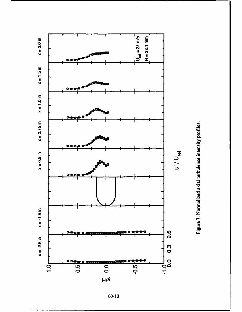
-S I I .
an
U7 z
0
x
60-13

0 141
CC')11
0O
c;Ic
x/
OUUU60u14
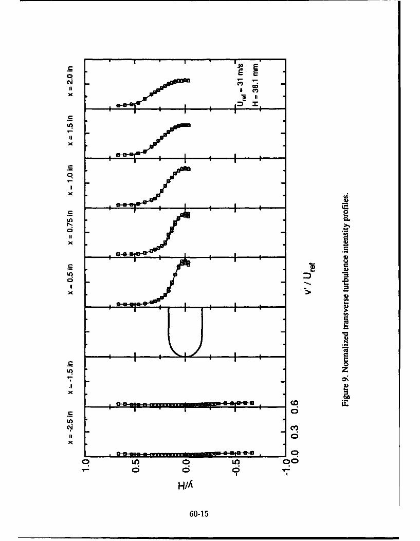
CC
IIt
In
x
13 0 A S-
In-
HI
60-1
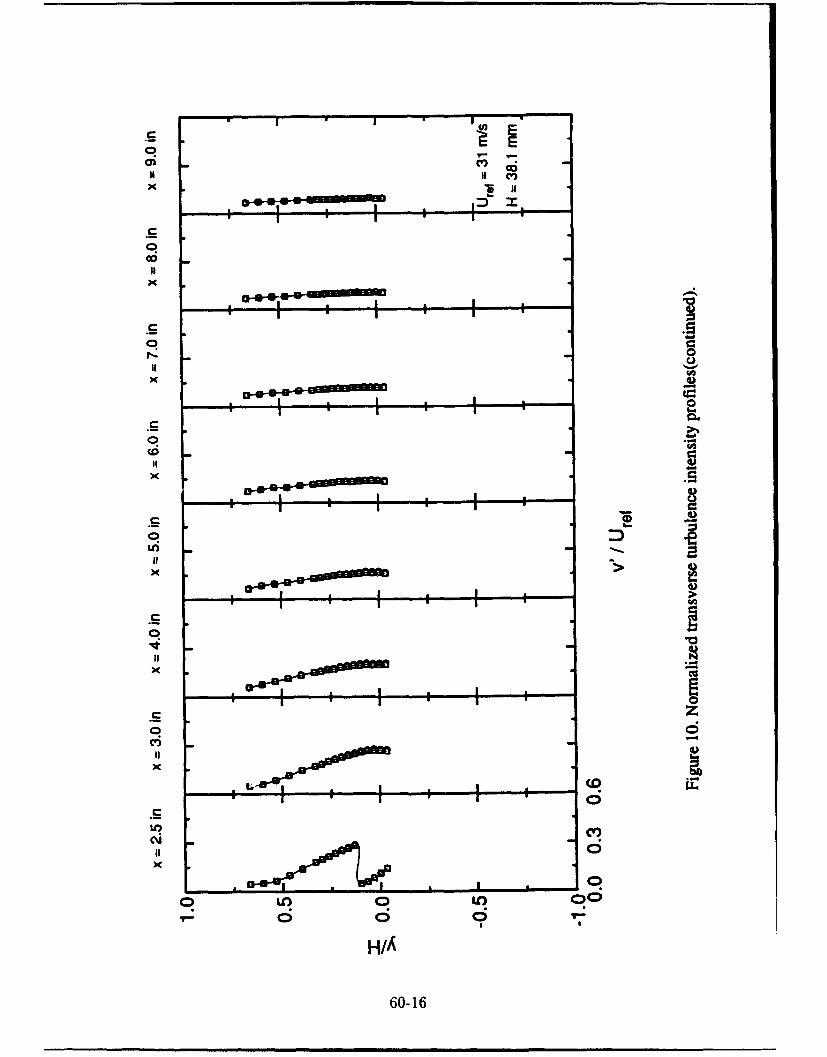
0)IIIit CV)
q~ininIf
H/
60-16
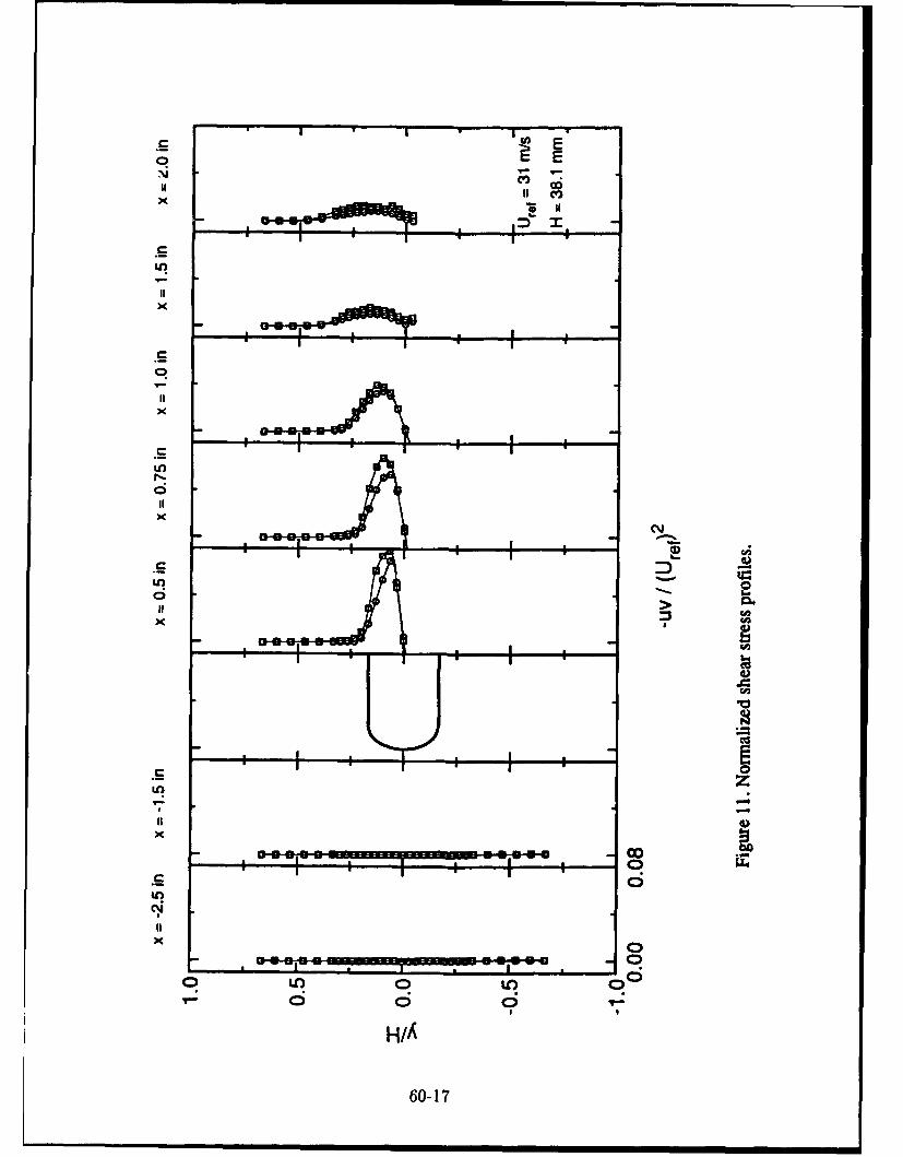
CV
M X
CC
Ui
Ar
xW
Ui
x
Dool4)
Ocz
II/
x _ _ _ _ __17

S E-
ci co C6,
IDI
I I601
x
It
x
9z
(0o
III
60-18

VAPORIZATION AND DECOMPOSITION OFTRICRESYL PHOSPRATE (TCP)
Christopher C. LAssociate Professor|Q
Department of Chemical and MaterialsEngineering
University of Dayton300 College Park Avenue
Dayton, OH 45469
Final Report for:Summer Research Program
Research & Development Laboratories
Sponsored by:Air Force Office of Scientific Research
Wright Patterson Air Force Base, Dayton, OH
August 1993
Laboratory Focal Point: f,' AUI qRobert L. Wright Jr. -/
Senior Project Engineer, WL/POSLWPAFB,OH 45433-6563
61-1

VAPORIZATION AND- DECOMPOSITION OFTRICRESYL PHOSPHATE(TCP)
Christopher C. LuAssociate Professor
Department of Chemical and MaterialsEngineering
University of Dayton
ABSTRACT
The boiling point of tricresyl phosphate (TCP) was estimatedto be 440*C at atmospheric pressure using the Clausius-Clapeyronequation, and was observed to be between 420*C and 435'C bydistilling a commercial grade TCP at atmospheric pressure.Experiments were conducted to study the rheological changes,viscosity and molecular weight by heating a commercial grade TCPin open and sealed tubes between 2500 C and 480 0 C in both dry airand nitrogen environments. It was found that below 380 0 C, boththe viscosity and the molecular weight increased significantlywith temperature in dry air, while the changes were very minor innitrogen. Above 4500 C, the TCP solution decomposed in both airand nitrogen with decreases in molecular weight and viscosity.Between 3900C and 4101C, the molecular weight began to decreasewhile the viscosity continued to increase. We suggest that thisis a transition region where TCP molecular chains begin to breakand evaporation begins to occur.
61-2

VAPORIZATION AND DECOMPOSITION OF
TRICRESYL PHOSPHATE(TCP)
INTRODUCTION
Tricresyl phosphate has long been used as an anti-wearadditive for turbine engine lubricants. Recently, Wedeven(Ref.1) conducted a traction study using a rotating ball and disctribometer and found that by using TCP vapor as a lubricant withdry air or nitrogen as a delivery gases, the traction coefficientcan be maintained at a range of 0.04 to 0.08 over a temperaturerange of 500 to 6700 C. Klaus, et al. (Ref.2) reported that thedeposition rate of TCP vapor condensates on iron and stainlesssteel surfaces increased when temperature increased from 500 to7000 C.
The potential application of vapor lubricants in advanced,high temperature engines appears promising, and furtherunderstanding of the physical and chemical behaviors of TCP inthe liquid and vapor phases is needed. Lu (Ref.3) used thermo-gravimetric analysis(TGA), differential scanning calorimetry(DSC), and gel permeation chromatography (GPC) to conduct thermalanalysis and molecular weight distribution studies for the TCPsolution, and found that the molecular weight of the solutionincreased with temperature at a range of 175 to 304 0 C in anoxygen environment. These results agree with the results of thisstudy that both molecular weight and viscosity increasedsignificantly below 380 0C with temperature under dry air. Thepurpose of this study is mainly twofold: (1) to determinetemperature ranges where the TCP solution begins to evaporate andto decompose, and (2) to observe the rheological changes of TCP,such as molecular weight distribution and viscosity, for thesetemperature ranges. To accomplish these goals, a theoreticalapproach was taken to calculate the vapor pressure of TCP, andseveral experiments were conducted to observe the physical andrheological changes of the TCP solution at elevated temperatures.
61-3

PROCEDURES AND RESULTS
1. VAPOR PRESSURE AND TEMPERATUREThe Clausius-Clapeyron equation was used to calculate the
vapor pressure of TCP between one and two atmospheres,
ln pv, - + BRT
where pv is a vapor pressure with units of mmHg, AH* is the heatof vaporization in units of cal/gm, R is the gas constant equalto 1.987 cal/(mole.K), and B is a constant calculated as a valueof 18.186 for the units used. The physical properties of TCP aregiven as: boiling point - 265*C at 10 mm Hg, and heat ofvaporization - 44.5 cal/g (Ref. 4), while the boiling point of p-tricresyl phosphate is 410 0C at atmospheric pressure (Ref. 5).Table 1 compares our results with the literature values.
Table 1. Vapor Pressure Temperature Relationship for TCPPV T
10 265 (90% mixture of isomers, Ref. 4)760 441 (this study)760 410 (p- TCP, Ref. 5)
1520 487 (this study)
The above values are plotted on a semi-log scale for pv vs1/T(OK) and the result is shown as a straight line in Figure 1.
1.000E+04
1.OOOE+03
1.000E+02
1.OOOE+001.000E+00
0 0.5 1 1.5 2
I/T(K) (IE-3)
Fig.1:Vapor Pressure for TCP
61-4
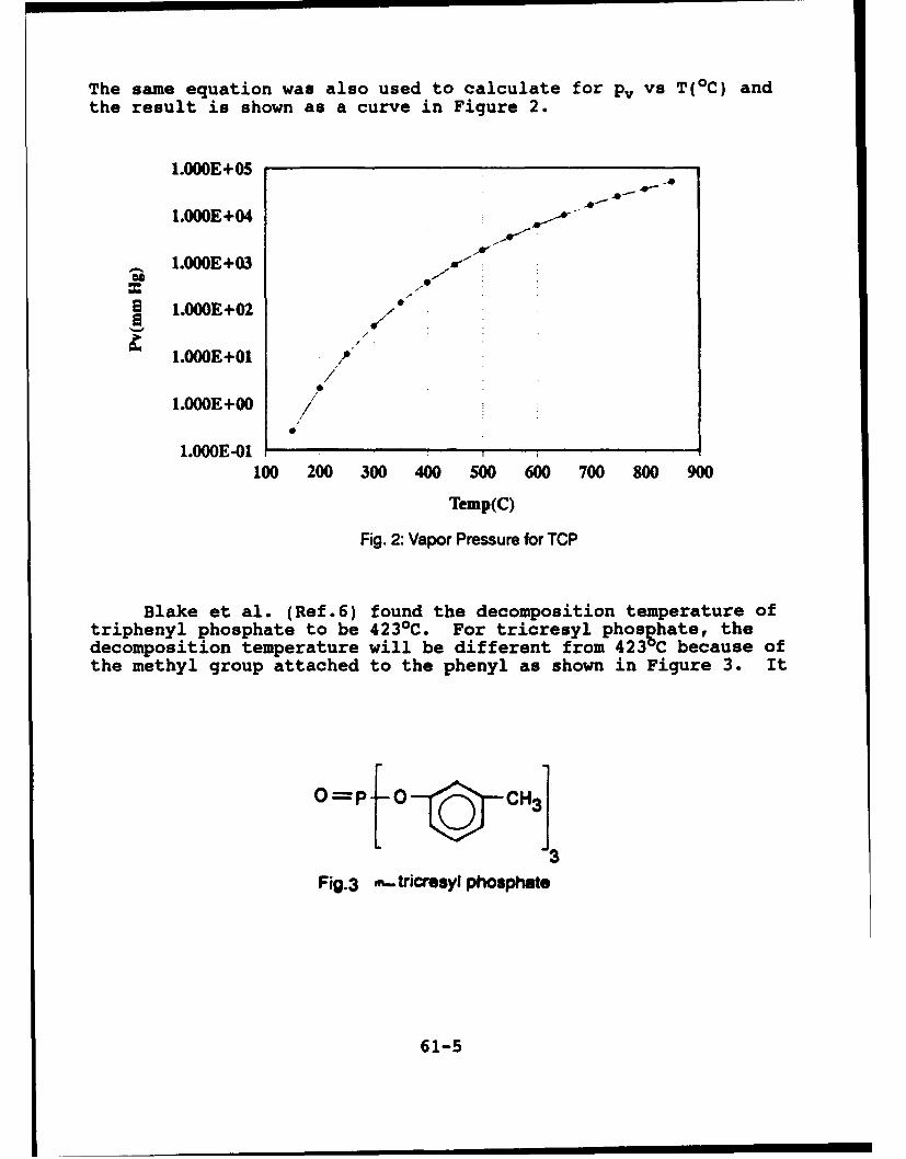
The same equation was also used to calculate for pv vs T(°C) andthe result is shown as a curve in Figure 2.
1.OOOE+05AP"
m..--
1.000E+04
1.OOOE+03
1.OOOE+02 "
/1.000E+01
1.OOOE+00 "
1.OOOE-01100 200 300 400 500 600 700 800 900
Temp(C)
Fig. 2: Vapor Pressure for TCP
Blake et al. (Ref.6) found the decomposition temperature oftriphenyl phosphate to be 423 0 C. For tricresyl phosphate, thedecomposition temperature will be different from 423 0C because ofthe methyl group attached to the phenyl as shown in Figure 3. It
O=Pf.-O--O-CH3]
-3Fig.3 ,a-tricresyl phosphate
61-5
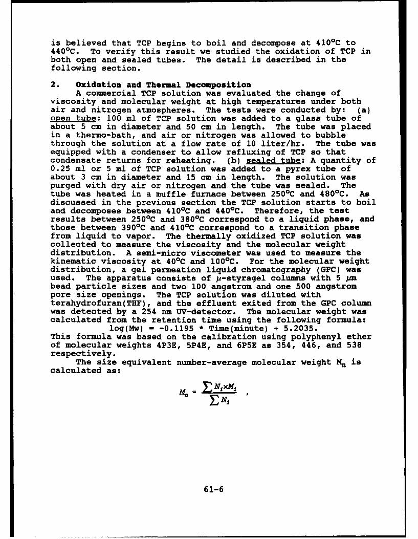
is believed that TCP begins to boil and decompose at 410*C to440 0 C. To verify this result we studied the oxidation of TCP inboth open and sealed tubes. The detail is described in thefollowing section.
2. Oxidation and Thermal DecompositionA commercial TCP solution was evaluated the change of
viscosity and molecular weight at high temperatures under bothair and nitrogen atmospheres. The tests were conducted by: (a)open tube: 100 ml of TCP solution was added to a glass tube ofabout 5 cm in diameter and 50 cm in length. The tube was placedin a thermo-bath, and air or nitrogen was allowed to bubblethrough the solution at a flow rate of 10 liter/hr. The tube wasequipped with a condenser to allow refluxing of TCP so thatcondensate returns for reheating. (b) sealed tube: A quantity of0.25 ml or 5 ml of TCP solution was added to a pyrex tube ofabout 3 cm in diameter and 15 cm in length. The solution waspurged with dry air or nitrogen and the tube was sealed. Thetube was heated in a muffle furnace between 2500 C and 480 0 C. Asdiscussed in the previous section the TCP solution starts to boiland decomposes between 410 0C and 440 0 C. Therefore, the testresults between 250°C and 380 0 C correspond to a liquid phase, andthose between 390 0C and 4100 C correspond to a transition phasefrom liquid to vapor. The thermally oxidized TCP solution wascollected to measure the viscosity and the molecular weightdistribution. A semi-micro viscometer was used to measure thekinematic viscosity at 40 0 C and 100 0 C. For the molecular weightdistribution, a gel permeation liquid chromatography (GPC) wasused. The apparatus consists of p-styragel columns with 5 pmbead particle sizes and two 100 angstrom and one 500 angstrompore size openings. The TCP solution was diluted withterahydrofuran(THF), and the effluent exited from the GPC columnwas detected by a 254 nm UV-detector. The molecular weight wascalculated from the retention time using the following formula:
log(Mw) = -0.1195 * Time(minute) + 5.2035.This formula was based on the calibration using polyphenyl etherof molecular weights 4P3E, 5P4E, and 6P5E as 354, 446, and 538respectively.
The size equivalent number-average molecular weight Mn iscalculated as:
61-6
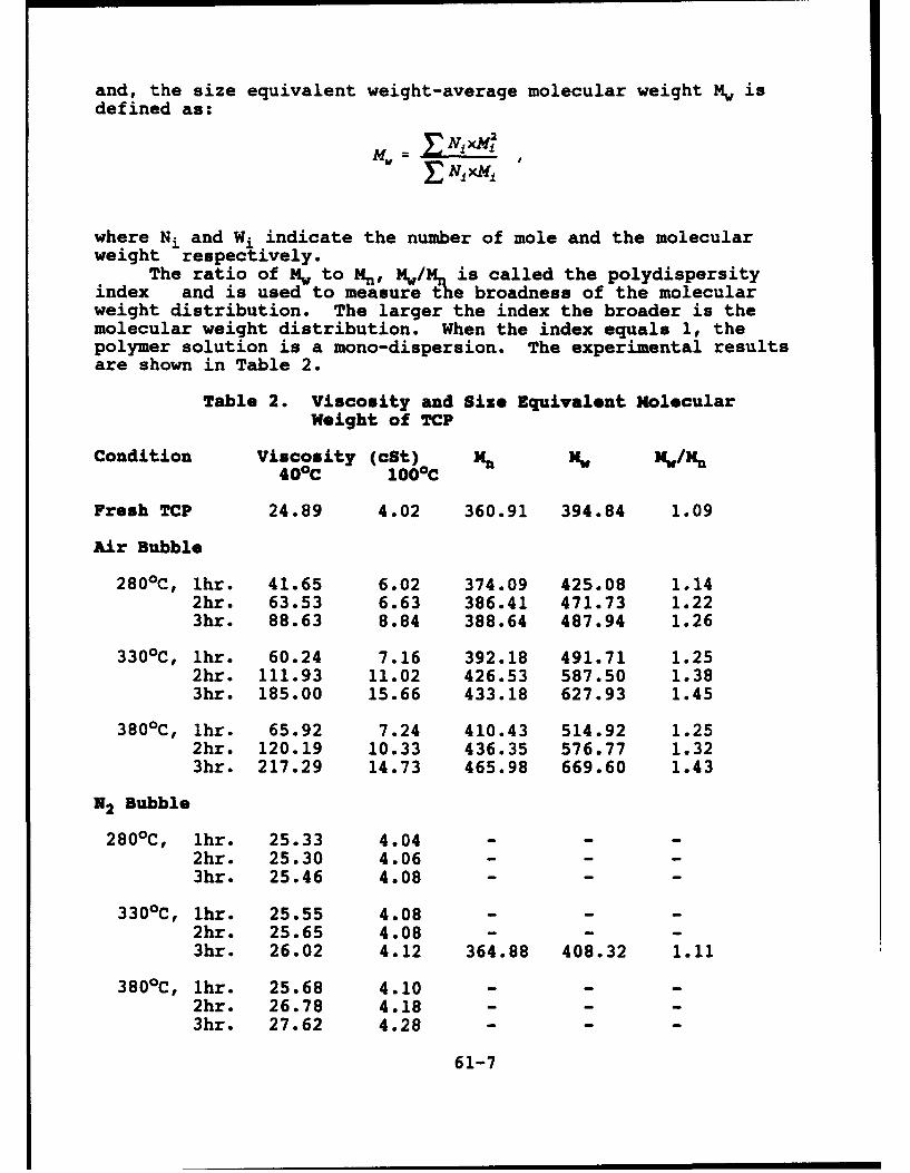
and, the size equivalent weight-average molecular weight Mw isdefined as:
rNI XMJ2
where Ni and Wi indicate the number of mole and the molecularweight respectively.
The ratio of Mw to Mn, Mw/Mn is called the polydispersityindex and is used to measure the broadness of the molecularweight distribution. The larger the index the broader is themolecular weight distribution. When the index equals 1, thepolymer solution is a mono-dispersion. The experimental resultsare shown in Table 2.
Table 2. Viscosity and Size Equivalent MolecularWeight of TCP
Condition Viscosity (cSt) Nn Mw Mw/Mn
40 0 C 1000C
Fresh TCP 24.89 4.02 360.91 394.84 1.09
Air Bubble
2800 C, 1hr. 41.65 6.02 374.09 425.08 1.142hr. 63.53 6.63 386.41 471.73 1.223hr. 88.63 8.84 388.64 487.94 1.26
330 0 C, 1hr. 60.24 7.16 392.18 491.71 1.252hr. 111.93 11.02 426.53 587.50 1.383hr. 185.00 15.66 433.18 627.93 1.45
380 0 C, lhr. 65.92 7.24 410.43 514.92 1.252hr. 120.19 10.33 436.35 576.77 1.323hr. 217.29 14.73 465.98 669.60 1.43
N2 Bubble
280°C, lhr. 25.33 4.04 - - -2hr. 25.30 4.06 - - -3hr. 25.46 4.08 - - -
3300 C, 1hr. 25.55 4.08 - - -2hr. 25.65 4.08 - - -3hr. 26.02 4.12 364.88 408.32 1.11
3800 C, 1hr. 25.68 4.10 - - -2hr. 26.78 4.18 - - -3hr. 27.62 4.28 - - -
61-7

4060 C, 1hr. 26.04 - 360.03 418.49 1.162hr. 27.42 - 374.85 424.23 1.133hr. 28.88 - 375.68 425.92 1.138hr. 38.19 - 384.70 431.84 1.12
Air Bomb
250 0 C, 1hr. 24.71 4.02 366.68 406.25 1.112hr. 29.07 16.79 364.67 401.32 1.10
345 0 C, 1hr. 35.35 5.24 359.24 417.69 1.162hr. 40.70 5.71 363.24 425.78 1.173hr. 43.55 6.30 374.24 451.91 1.21
390 0 C .Shr. 58.82 - 367.03 484.84 1.321hr. 75.32 - 362.84 479.65 1.322hr. 98.63 - 314.55 435.70 1.38
4100 C, .5hr. 62.34 - 340.80 465.74 1.371hr. 111.35 - 319.57 458.50 1.432hr. - - 257.60 381.53 1.48
450 0 C (0.25 ml TCP)* 1hr. - - 261.61 396.15 1.51* 2hr. - - 224.89 410.87 1.83
460 0 C (5 ml TCP)* 2hr. - - 241.27 487.97 2.02
N2 Bomb
450 0 C (0.25 ml TCP)* 1hr. - - 343.86 433.04 1.26* 2hr. - - 238.85 408.03 1.71
460 0 C (5 ml TCP)* 1hr. - - 220.37 395.2 1.79* 2hr. - - 217.68 395.8 1.82** 5hr. 1.11 - 245.65 526.65 2.14
480 0 C** 6hr. 1.01 - 250.45 531.37 2.12
* Sample was too thick and quantity was too small to test.** Sample was heated slowly.
61-8

DISCUSSIONS
The above results show : (1) at 2800 C, 330 0 C, and 380'C, bothviscosity and molecular weight of TCP solution substantially increasewith both the temperature and heating time in the air environment.The molecular weight distribution also becomes broader. In thenitrogen environment, however, these increases are relatively minor.This suggests that the polymerization reaction takes place in thepresence of oxygen. It was also discussed by Lu (Ref.3) that theoxidation reaction enhanced the polymerization of TCP solution at atemperature range of 175*C to 3040 C; (2) at 250*C, and 345 0 C "airbomb" condition, both molecular weight and viscosity increase, butonly slightly. It is evident that the amount of oxygen inside thesealed tube was not enough to continue the oxidation reaction; (3) at450 0 C, 4600, and 4800 C, we observed that the TCP solution quicklydecomposed and formed a dark residue inside the sealed tube under bothdry air and nitrogen conditions. The viscosity test was not runbecause of an insufficient amount of TCP solution was left inside thetube. However, the GPC test shows that during the first two hours,the number average molecular weight, Mn, significantly decreases, theweight average molecular weight, Mw, only slightly increases, and themolecular weight distribution becomes slightly broader. This suggeststhat at the beginning of thermal decomposition, the binding chains ofTCP molecules break and form smaller molecular weight species.However, when the temperature is slowly increased to 4600 C and 4800Cin 5 and 6 hours, these small molecules begin to combine to formlarger molecules. The results are shown at 460 0 C and 480*C for 5 and6 hours runs, where the weight average molecular weight, Mw ,increases to around 530 and the molecular weight distribution furtherwidens to 2.1; (4) at 406 0 C with nitrogen bubbling, both viscosity andmolecular weight gradually increase without suffering thermaldecomposition, which suggests that 406 0 C is still below thedecomposition temperature; (5) at 390 0 C and 410 0 C "air bomb"conditions, viscosity increased by increasing the heating time from1/2 hour to 2 hours. However, both M. and Mw decreased with theheating time. The decrease of molecular weight was rather minor at390 0 C, especially up to one hour of heating time, but it was rathersevere at 4100 C. These suggest that the range between 3900 C and 4100Cis the transition temperature range where some molecules chains maybegin to break and some degree of polymerization may still take place.The above experimental data were plotted based on viscosity/Mn andviscosity/Mw and are shown in Figures 4 and 5.
61-9
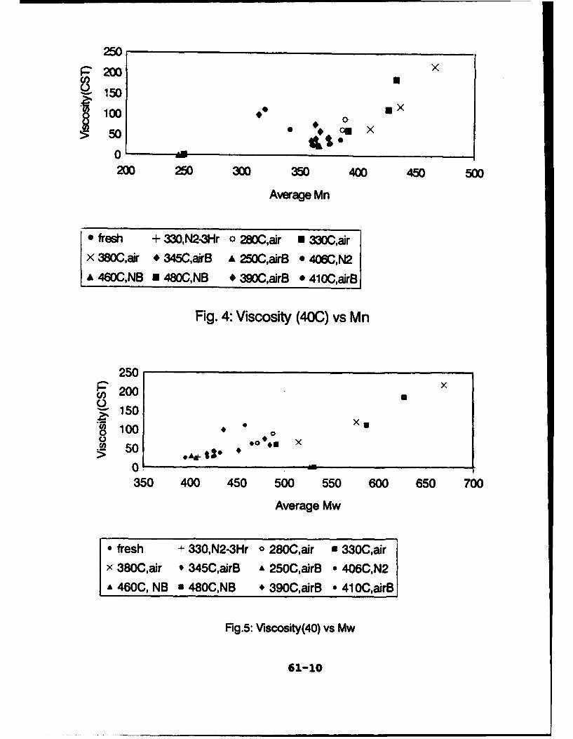
250
P 200 x
-150U
0 AM
200 2W0 305 400 450%0
Average Mn
*fresh + 330,N2-3Hr 0 280C,air * 3300,airX 380C,air * 345C,airB A250C,airB * 4o6C,N2,A 460CNB * 480C,NB *3=0,airB e 410C,airB
Fig. 4: Viscosity (400) vs Mn
250~200X
Q1500 100 0E
00 A
350 400 450 500 550 600 650 700
Average Mw
fresh +- 330,N2-3Hr * 280C,air *3300,air
x 380C,air # 345C,airB A 2500,airB *4060,N2
A 4600, NB a 480C,NB 4 3900,airB *41 OC,airB
Fig.5: Viscosity(40) vs Mw
61-10

CONCLUSIONS
Commercial tricresyl phosphate (TCP) solution boils at atemperature of about 420 0 C to 4351C, and thermally decomposes at about450'C. At a temperature between 390 0 C and 410 0 C, some molecularchains may break and some polymer molecules may still form. Theviscosity increases with the heating time and the molecular weightbegins to decrease. Below 380 0 C, the molecular weight and theviscosity of the TCP solution increase significantly with bothtemperature and heating time in the air environment, and the molecularweight distribution also widens. In the nitrogen environment, thesechanges are minimal. The results suggest that the oxidation reactionenhances the TCP polymerization below the boiling temperature. Above4500 C, the TCP will decompose thermally under both oxygen and nitrogenenvironments.
6-11

ACKNOWLEDGEMENTS
The author thanks the Air Force Office of Scientific Research(AFSOR) 1993 Summer Research Program and the Lubrication Branch ofWright Patterson Air Force Base for fund and facilities available forthis project. Thanks also go to Michael A. Keller and Mary Borchersfrom the University of Dayton Research Institute for generating themolecular weight distribution and viscosity data for this study.
61-12

REFERENCES
1. Wedeven, L.D., "Extended Temperature Range Lubrication withVaporized Liquids," Wedeven Associates,Inc. Technical Report, WL-TR-91-2034, March 6, 1991.
2. Klaus,E.E., Dada, J.L., and Naidu,S.K.,"Formation ofLubricating Films at Elevated Temperature From the GasPhase," NIST Special Publication 774, Sept.1988.
3. Lu, C."Thermal Analysis and Molecular Weight Distribution ofTriaryl Phosphates," Final Report for Summer ResearchProgram, Lubrication Branch, Aero Propulsion and PowerDirectorate, Wright Laboratory (AFMC), Sept. 1992.
4. Aldrich, Catalog Handbook of Fine Chemicals ,1992-1993.
5. CRC Handbook of Chemistry and Physics, 60th edition, CRCPress,Inc.
6. Blake, E.S., Hammann, W.C., Edwards, J.W.,Reichard,T.E. andOrt, M.R.,"Thermal Stability as a Function of ChemicalStructure, "Journal of Chemical and Engineering Data," Vol. 6, No. 1,Jan. 1961.
61-13

DESIGN OF A STABILIZED CENTER-BODY COMBUSTOR
S. RAGtIUAssistant Professor
Department of Mechanical Engineering
State University of New YorkStony Brook, New York 11794-2300
Final Report for:
Summer Faculty Research ProgramWright Research and Development LaboratoryWright Patterson Air Force Base, Ohio 45433
Spor,4zred by:
Air Force Office of Scientific ResearchBoiling Air Force Base, Washington. D.C.
September 1993
62-1

DESIGN OF A STABILIZED CENTER-BODY COMBUSTOR
S. RAGHUAssistant Professor
Department of Mechanical EngineeringState University of New York
Stony Brook, New York 11794-2300
ABSTRACT
The objective of the present work was to design a stable, low NO1, high performance center-body combustor.Five different center-body configurations were studied experimentally to determine their performancecharacteristics under various operating conditions. The lean blow out limit in all the cases was found to bearound 0.03 which is an order of magnitude lower than the present combustors in use. A multiple air-fuel jetconfiguration with independent control of the primary air showed a promising over-all performance andfurther tests are in progress to determine their emissions characteristics. Increased and controlled mixing wasfound to be the key factor in extending the operating range of the combustor.
62-2

DESIGN OF A STABILIZED CENTER-BODY COMBUSTOR
S. RAGHU
I. INTRODUCTION
A good stability and performance of the combustion system under a wide range of operating conditions is
necessary to meet the demands of both military and commercial gas turbines. In military applications, the
maneuverability of the aircraft is increased if large changes in the thrust can be brought about without flame-
out conditions of the engines. In commercial aircrafts efficient, low NOx engines are necessary to meet the
increasing demands of environmental regulations. There has recently been a surge of activity on the design of
new combustors whose main goal is to achieve the above two objectives by increased mixing as well as staged
combustion [11,121,131 & 141. Increased mixing reduces locally hot spots that are conducive to NOx formations.
Staged combustion [1] allows non-stoichiometric combustion, i.e., an initial stage of rich burning and a second
stage of lean burning and in both these combustion processes the NO, formation is considerably less than the
stoichiometric burning.
Some important requirements of a gas turbine combustor are:
1. Flame stabilization
2. A low lean blow out limit (stable operation at low loading)
3. A high rich blow out limit (stable operation at high loading)
4. Low NOx emissions
5. Desirable temperature profiles at the end of the combustion chamber
6. Low pressure drop across the combustor
All these requirements, except for the pressure drop. depend on the efficiency of mixing in one way or another.
Mixing of air and fuel is necessary in the primary combustion zone, while mixing of the high temperature
62-3

combustion products with the dilution air is necessary downstream of the combustion zone. Control of the
mixing process is therefore essential in order to control the stability limits of combustion as well as the
emissions of undesirable NOx and THCs.
This work is aimed at developing new concepts for combustor design keeping in mind the above requirements
and constraints of a practical combustor. In particular, the present objectives are to increase the range of
stable operation of a combustor and the reduction of the NOx and THC emissions through proper control of
the mixing processes in the combustor. Studies of some new configurations for the center body designed for
this purpose are described in this report.
II. METHODOLOGY
Several configurations of the center-body designed to achieve the fore-mentioned goals were experimented with
for comparison of their performance. Figure 1 shows the new center-body combustor configurations used in
the present experiments. Important features of each of these are described in the following paragraphs.
Configuration I
It consists of a circular disk with a central fuel tube of 89 mm length and 12.7 mm diameter extending into
the recirculating zone. The blockage ratio between the primary air duct and the disk is 78%. The fuel is
introduced into the recirculation zone through a circular array of eight holes of size 2 mm diameter drilled
in the extension tube and located 38 mm downstream from the disk. The fuel jets are directed at an angle of
45 degrees inclined back towards the circular disk. The objective of these directed fuel jets is to distribute the
fuel into the recirculation zone.
Configuration 2
Fuel in this case is introduced through 8 radial holes of size 1 mm located at the base of the extension piece
of the same length as configuration 1 (89 mm). Fuel from these jets flow outward on the disk so that they are
62-4

entrained into the annular flow and transported back into the recirculation zone.
Configuration 3
In this configuration an additional disk of 57 mm diameter was placed at a height of 64 mm from the base of
the central tube in order to increase the recirculation by directing some of the annular flow into the
recirculation zone. Fuel is introduced in the same way as configuration 3.
Configuration 4
This is similar to (1) except that the fuel is introduced at two locations --- one at the base of the disk through
eight 1.5 mm diameter holes and the other at a height of 38 mm and directed 45 degrees upstream with the
aim of obtaining a more uniform distribution of the fuel in the recirculation zone.
Configuration 5
This was designed after preliminary tests were run on the previous designs. Additional air into the recirculation
zone is provided by a separate source than the primary entrained air. It consists of a central manifold with 8
fuel holes of 1.75 mm diameter and concentric holes for air, with a row on the inner side and a row on the
outer side of the fuel tubes. The 8 inner air holes have a diameter of 2.2 mm and the outer holes are 2.3 mm
diameter and sixteen in number. All these are directed into the recirculating zone. Thus, each fuel jet is
surrounded by 4 air jets in order to enhance the mixing of the fuel and the air. The air to these jets are
supplied from a source separate from the primary air so that the local mixing can be monitored. With the same
exit velocities for the fuel and the air jets, the air fuel ratio based on the volumetric flow rates is about 5. This
amount of air in addition to the recirculation air should aid in the stoichiometric combustion for all fuel flow
rates. Also, this configuration can sustain combustion with the complete cut-off of primary air thus acting like
a pilot flame.
62-5

I11. EXPERIMENTS
The experiments were conducted in the combustion facility at the WRDC. The details of the facility are
described in [5]. Briefly., it consists of a chamber with annular air flow with provision for holding any center-
body configuration. The lean blow out limit, the onset of the blue flame and the flame height was measured
for all the above configurations for different primary air flow rates. The flame height was directly measured
and the equivalence ratios were calculated based on the total amount of air and the fuel, both of which were
monitored by flow meters. The center line temperature was measured at a downstream distance of 20 cm (8")
from the disk. The pressure drop across the disk was measured by a water manometer.
IV. RESULTS AND DISCUSSION
Figure 2 shows the lean blow out limit for the various configurations. The equivalence ratio corresponding
to LBO for all the configurations lie within 0.02 -- 0.04, the configuration 1 having the higher LBO limit while
the configuration 2 has the lower LBO limit. This entire range of equivalence ratios are of an order of
magnitude lower than those of the current center body combustors (see for eg., [11-[41).
Another aspect of performance is the stoichiometric burning of the fuel in the combustor. Figure 3 shows the
onset of blue flame for two configurations. For both cases, the blue flame occurs at a very low equivalence
ratio indicating limited supply of oxygen in the recirculation at higher fuel flow rates. The other configurations
also showed similar trends but the data was not recorded.
The occurrence of sooty flames even at low equivalence ratios indicates that there is not sufficient flow of the
primary air into the recirculation zone and also limited entrainment of the combustion products back into the
primary flow. The former depends on the strength of the recirculation while the latter depends on the mixing
characteristics of the separated shear layer from the disk. Since for a given geometry both these quantities are
fixed, higher fuel flow rates result in locally rich burning of the fuel. In order to promote larger entrainment.
a disk with 8 azimuthal lobes was also fabricated. Although this yielded a slightly better performance, it wa%
62-6

not significant enough to warrant further studies.
Figure 4 shows the center line temperature measured at a downstream location of 8" from the disk for the
different configurations. The centerline temperature increases with increasing equivalence ratio as can be
expected. However. the temperature appears to be independent of the air flow rates and this can be
particularly seen for the cases (1) and (2). This is possibly due to the limited amount of entrainment in the
recirculation zone and the limited amount of mixing along the axis of the disk.
Configuration 5:
A more detailed study of this configuration was undertaken since it was designed to overcome the
shortcomings of the previous configurations. The present discussion is based on the results available so far.
Four parameters were varied: the annular air, the primary air (air from the jet-nozzles, the fuel flow rate and
the height of the center-body.
1. Visual observations of the flame
The flame exhibits excellent stability over most of the run conditions. At times an azimuthal rotation of the
flame was observed but this did not lead to flame blow out. Several factors that could trigger this azimuthal
rotation need to be examined in detail such as the flip-flopping of the air/fuel jets, asymmetry in the annular
flow, helical instability of the disk wake or the center-body wake, non-uniformity in the air/fuel injection, etc.
2. Lean Blow Out limits for different air flow rates
2a. Varying the annular air flow rate
Figure 5 shows the lean blow out limit expressed in terms of the overall equivalence ratio plotted as a function
of the annular air flow. The overall equivalence ratio is calculated using the total amount of air (annular air
+ primary air) supplied to the combustor. In all the experiments the primary air was fixed at 99 slpm and the
62-7

fuel and the annular air flow rates were varied. The values of the equivalence ratio for lean blow out are
around 0.03 and hence an order of magnitude lower than that of the present combustors. A local equivalence
ratio in the primary combustion zone (primary equivalence ratio) based on the primary air injected and the
fraction of the air entrained into the primary zone from the annular air flow was also calculated. The entrained
air was assumed to be a fraction of the annular air. Based on the previous experience of lean blow out values
of bluff-body combustors, entrainment ratios of 5 % and 7 % were assumed for calculations and the results
are plotted in
figure 6. The equivalence ratio appears to asymptote towards a value of about 0.4 based on 5% entrainment
and is slightly lower for a 7% entrainment. Since the flammability limit for propane in a well-stirred reactor
is 0.5. the results appear to be consistent to the extent that the equivalence ratio is below the flammability
limit.
2b. Effect of varying the primary air
In this set of experiments, the annular air was fixed at 2000 slpm and the lean blow out limit was determined
for varying amount of primary air and is shown in figure 7. The primary equivalence ratio is again in the
flammability limits for propane and is consistent with the previous set of data.
3. Performance at high loading
The fuel velocity at 20 slpm (maximum flow rate tested with the other configurations) is approximately 17 m/s
and the stoichiometric air necessary for combustion is about 320 slpm. If all the combustion air is supplied
by the manifold, the velocity of air is 55 m/s and this is approximately half the primary air velocity. This
velocity is also of the same order as the reverse flow velocity in the recirculation zone. Thus even at high
loadings, there is local stoichiometric burning and hence a high combustion efficiency is maintained in the
burner. Visual observation of the flame indicated this trend, i.e, by increasing the amount of primary air
injection, a blue flame was obtained even for the highest fuel loading.
62-8

.4. Performance at low loadine
At very low thermal loading, the requirement of the combustor is to sustain a stable flame without blow out
or in other words, we would like to extend the lean blow out limit of the combustor. This is easily achieved
by cutting off the manifold air supply and this configuration is then similar to the other configurations
discussed before in which we saw that the lean blow out was extended by an order of magnitude compared to
the conventional burners.
5. Effect of varying the height of the center-body from the disk
The variation of the overall equivalence ratio and the primary equivalence ratio for LBO for different heights
of the center-body are shown in figures 8 and 9 respectively. The lean blow limit rapidly increases with the
height in both the figures. Visual observation indicated a detached and unstable flame for the higher center-
body locations. It is possible that the mixing in the primary zone is inefficient due to a weaker recirculation
zone.
6. Rich-lean combustion to reduce NO,
By controlling the amount of primary air it was possible to obtain a rich (yellow colored flame) in the vortex
core and a blue flame both in the disk shear layer as well as in the rest of the primary zone. Since the fuel and
the combustion products in the rich burning region (vortex core) are later entrained into the separating shear
layer of the disk, a lean combustion occurs in the shear layer zone. Thus it is possible to reduce the NO,
formation which is maximum at the stoichiometric combustion regime. Emissions tests Will be conducted in
the near future to examine this conjecture.
7. Thermal loading of the combustor/center-body
Another problem encountered with the previous configurations was the excessive heating r he center-body
extension tube due to the flame. At higher fuel flow rates the center body was red hot thus, reducing the life
time of the tube. The present design has both air and fuel flowing continuously through the center-body in
62-9

order to keep it at lower temperatures. Except for the cases of either no primary air injection or verey low air
flows. the center-body appeared to be sufficiently cooled by the air/fuel flow.
S. Emission tests
It is planned to evaluate the combustion efficiency and the NO, emissions in the near future.
V. CONCLUSIONS
The objective of the present work was to design a stable, low NO, high performance center-body combustor.
Five different center-body configurations were studied experimentally to determine their performance
characteristics under various operating conditions. The lean blow out limit was found to be around 0.03 which
is an order of magnitude lower than the present combustors in use. A configuration with independent control
of the primary air and hence primary mixing (configuration 5) also had excellent performance at higher fuel
loading and further tests are in progress to determine their emissions characteristics. Increased and controlled
mixing was found to be the key factor that governs the performance of a combustor.
VI. ACKNOWLEDGEMENTS
The author would like to acknowledge the help of Dr. K.-Y. I-Isu (Systems Research Laboratories) in
conducting the experiments. This project was initiated by Dr. W.M. Roquemore and his continued interest and
suggestions at all stages of this work is gratefully acknowledged.
VII. REFERENCES
1. Micklow, G.J., Roychoudhury, S., Nguyen, H.L and Cline, M.C. (1993), Emissions reduction by varying the
swirler airflow split in advanced gas turbine combustors, J. Engrg for Gas Turb. and Power, Trans. ASME. vol.
115, pp. 563-569.
2. McVey, J.B., Padget, F.C., Rosfiord, T.J., Hu, A.S., Peracchio, A.A., Schlein, B and Tegel, D.R., (1991).
Evaluation of low-NO, combustor concepts for aeroderivative gas turbine engines, J. Engrg for Gas Turb. and
62-10

Power. Trans. ASME. vol. 115, pp. 581-587.
3. Cowell. L.H. and Smith. K.O. (1993). Development of a liquid-fueled. lean-premixed gas turbine combustor.
J. Engrg for Gas Turb. and Power. Trans. ASME. vol. 115. pp. 554-562.
4. Aigner. M. and Muller, G. (1993), Second-generation low-emission combustors for ABB gas turbines: Field
measurements with GTI IN-EV, J. Engrg for Gas Turb. and Power. Trans. ASME. vol. 115. pp. 533-536.
5. Roquemore. W.M.. Tankin. R.S., Chiu, H.H. and Lottes, S.A. (1986), A study of bluff-body combustor using
laser sheet lighting, Exp. Fluids, vol. 4, pp. 205-213.
62-11
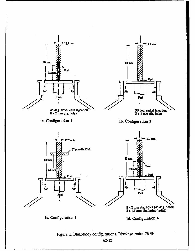
12.7 mm 12.7 mm
9mm 89 mm
31 Fuel
Fuel
Air LAir Air Air
Fuel FuelII
45 deg. downward injection 90 deg. radial injection8 x 2 mm dia. holes 8x1mm di m holes
la. Configuration 1 lb. Configuration 2
44! 1412.7 mm - 12.7 mm
I ~ ~57 mm dis. DiskI8.899mm 89 mm
AF~a
Fue I Fa
ir LAAir Ful Air
FueI I
8 x 2 mm dia. holes (45 deg. down)8 x 1.5 mm dia. holes (radial)
1c. Configuration 3 1d. Configuration 4
Figure 1. Bluff-body configurations. Blockage ratio: 76 %
62-12

FUEL HOLES
0 00o 49 0o qAIR HOLES
SECTON AT A-A 0 Q Q00° 0
A A
AIR I.FUEL
Figure le. Configuration 562-13

LBO data of 76 % Blockage Ratio (Nonconfined)0.06
o config. 1o3 config. 2
0.05 o config. 3 "p.@Hu2S)o X config. 4
S0.04 0o0 x 0 0
x.> 0.03 0
rC3 0oo
0.02 o o C3
x0 .0 1 . .I I , I I I , I I .I II '
0 500 1000 1500 2000 2500 3000 3500Air (slpm)
Figure 2. Lean blow-out limit for various configurations
LBO.data.1230.06
0.05 0
9x 0.04 0x 0
x. 0.03
.. '.o Configuration 1
0.02 a Configuration 40
x x PW LBO#30.01. I ...1 1 .... I .... , 1 1 .... 1,,,-I,,,,
0 500 1000 1500 2000 2500 3000 3500Air (slpm)
Figure 3. Onset of blue-flame for different configurations.
62-14

Nozzle #1 C.L. Temperature @ H =8800
700
600...!
L 500 :Mi
40 0 V ...
0+ 500' i300 0 1000air
1500O air200 i x 2000 airp I i + 2500 air
00"0 L ~o C30' 3000 air100 LLIW W,___
0 0.05 0.1 0.15 0.2 0.25 0.3 0.35
Equivalence Ratio
Configuration 1
Nozzle #2 C.L. Temperature @ H= 8800 7 r
700 -
6-00-
x :xi, 1 ^ 4,,x+
400 - -
3000 500 air
200 I 4A I ,l 1000 air0• 1500 air2 -x 2000 air
-100 + 2500 aira 3000 air
07 1L.1i___1___0 0.05 0.1 0.15 0.2 0.25 0.3 0.35
Equivalence Ratio
Configuration 2
Figure 4. Center-line temperature at 20 cm downstream distance
62-15

Nozzle #2 C.L. Temperature @ H = 8 "(with Top cap)
800
700600 ,i ,
500
L I
200-j COCI0 1000 air.cap,
100 'C3 2000 air.capo 3000 air.cap
0 i i0 0.05 0.1 0.15 0.2 0.25 0.3 0.35
Equivalence Ratio
Configuration 3
Nozzle #3 C.L. Temperature @ H =8800 -Ti'I _ ___
700 • 0
.600 x i
400 I 0
Ix
0 100o 0 air200 -- 2000air
1 00 . . x 3000 air100' -
0 0.1 0.2 0.3 0.4 0.5 0.6
Equivalence Ratio
Configuration 4
Figure 4 (contd). Center-line temperature at 20 cm downstream distance62-16

Overall eq. ratio vs Annular flow for LBO0.05 ,
S Phi, total
20 0.04
S S 0a 0.03
0
6~ 0.02i.
0 0.01
0
500 1000 1500 2000 2500 3000 3500
Annular air, slpm
Figure 5. Overall equivalence ratio for lean blow-out s annular air flow (Configuration 5)
Local Phi vs Annular Flow for LBO0.5
0 7%entairD S%entair
0.4 o
0.& 0.3 0
-0.2 r
0.1
0 I I
500 1000 1500 2000 2500 3000 3500Annular air, slpm
Figure 6. Primary equivalence ratio for lean blow-out vs annular air flow (Configuration 5)
62-17
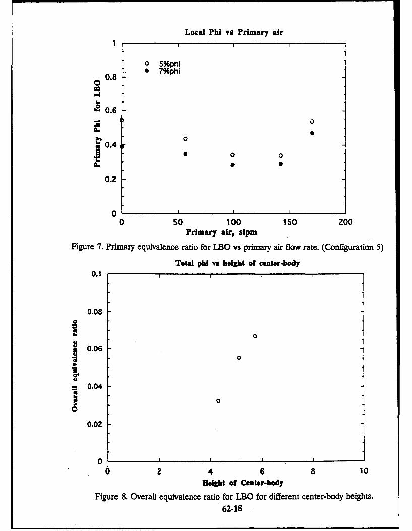
Local Phi vs Primary air
o 5%phi0 7%phi
0.8
0 0.60 0
A04 o
0.2
0 J0 50 100 150 200
Primary air, slpm
Figure 7. Primary equivalence ratio for LBO vs primary air flow rate. (Configuration 5)
Total phi vs height of center-body
0.1 ,
0.08
00
0.06Ii 0
- 0.046 0o
0.04
0
0 p I
0 2 4 6 8 10Height of Center-body
Figure 8. Overall equivalence ratio for LBO for different center-body heights.
62-18
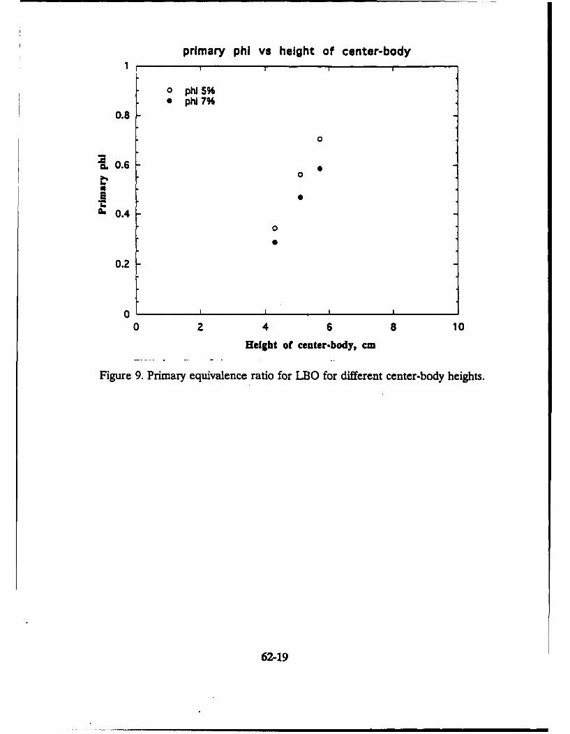
primary phi vs height of center-body1I I II
o phi 5%* phi 7%
0.8
0
10.6
'C
1 0.4
0.2
0 2 4 6 8 10
Height of center-body, cm
Figure 9. Primary equivalence ratio for LBO for different center-body heights.
62-19

Comprehensive Analysis of Switched Reluctance Machineby The Coupled Field and Circuit Modeling Method
Longya Xu
Assistant Professor
Department of Electrical Engineering
The Ohio State University
2015 Neil Avenue
Columbus, Ohio 43210
Final Report for:
Summer Research Program
Wright Laboratory
Sponsored by:
Air Force Office of Scientific Research
5800 Uplander Way
Culver City, CA 90230-6608
August. 1993
63-1

COMPREHENSIVE ANALYSIS OF SWITCHED RELUCTANCE MACHINE
BY THE COUPLED FIELD AND CIRCUIT MODELING METHOD
Longya XuAssistant Professor
Department of Electrical EngineeringThe Ohio State University
Abstract
One of the very important research topics in a switched reluctance machine (SRM)
system is its complicated dynamics under various transient or fault conditions. These
transients or faults impact not only the SRM magnetic field internally but also the associated
power control circuit externally. In this research project, a computer model including the
power electronic converter, control circuits and the nonlinear magnetic field of the SRM is
established. Finite element method is used to model the nonlinear magnetic field of the
SRM. The SRM field model is further tightly coupled to the circuit model of the overall
system. With simultaneous computation over the entire system including the SRM
magnetic field and power converter circuit, the proposed computer model provides a
powerful computer tool to investigate the SRM system extensively. Initial experimental
results are presented to validate the computer model.
63-2

Table of Contents
1. Introduction 4
2. Principle of Switched Reluctance Machine 5
3. Field and Circuit Combined Modeling Method 7
4. Results of Theoretical Analysis 11
5. Results of Experimental Testing 17
6. Conclusions and Future Work 18
References 20
63-3

1. Introduction
Although induction machine drives are still the workhorse of industry, the switched
reluctance machine (SRM) drive has been actively researched for more than a decade with
very promising results [1-31. The SRM has a simple and rugged construction as well asvery good overall performance over a wide torque-speed range [2]. Recently. doubly-
salient switched reluctance machines have been found to be an attractive alternative to more
conventional PM synchronous and induction machines in converter fed variable-speed
drives and generating systems.
The SRM, in effect, is an advanced type of stepping motor in which the current
waveform of the machine must be carefully programmed to extract the maximum
torque/ampere[41. The fundamental feature of this type of motor system is that the SRM
requires only unidirectional current and thus the converter topology and corresponding
switching algorithm of the power converter is greatly simplified. In addition, unidirectional
current of the SRM enables that the power circuit configuration is immuned from shooting-
through fault, which is a particularly attractive feature for high reliability in aerospace
applications.
While the recent work on SRMs are encouraging, the unresolved issues of system
transient performance and failure riding-through capability remain. These issues need to be
addressed and solved for applications requiring high reliability, such as aerospace
propulsion and generating systems. In this project, a new approach of modeling a SRM is
proposed and studied. In particular, the field analysis of the SRM by finite element
analysis is combined with the circuit analysis of the entire system. As a result, this coupled
field-circuit modeling method on the SRM will not only reveal the internal magnetic stress
of the SRM during the transient but also provide sufficient information regarding the
terminal dynamics of the system.
An experimental SRM has been chosen and the corresponding power converter
circuit has been set up to verify the proposed modeling method. The results from the
experimental SRM system are very close to those from the model prediction, indicating the
accuracy of the field-circuit model.
63-4

2. Principle of Switched Reluctance Machine
Electromechanical energy conversion in a SRM, ideally shown in Fig. l(a), is
accomplished by means of a time varying inductance due to the variation of the rotor
position. The physics of the model can also be represented by the simple circuit shown in
Fig. I(b).
S
,• !. L(Or) / L //•
D n6 .*u256
• W-;.v i•12 5i12vU'
Figure L.(a) Configuration and Idealized Inductance and Current of SRM
+
4 E
Figure 1.(b) Equivalent Circuit of the Idealized SRM
63-5

For simplicity of analysis, all the losses are neglected for the time being, and
therefore no resistance is involved in the circuit. The circuit is assumed to be fed with a
prescribed current as shown in Fig. 1(a) from the source and the inductance is time-
varying due to the rotor rotation. The flux linkage associated with the inductance L is X
and if saturation of the magnetic material is neglected, the flux linkage can be expressed as
X = L (Or) i
where L(O r) is only a function of rotor angle displacement (saturation neglected). The
induced voltage by the inductance is
E =ldt
.Ldi +i dL dOrdt dO r dt
The instantaneous power entering the circuit is
P = Ei
di ,,1dL=Li d + cOr --- (2)
where the rotor angular speed dOr/dt is assumed to be a constant. Wr. Replacing the first1 di2 a ndL I .2dL
term by 1 L-- and splitting the second term into two parts, (Or 1 )--- and • 1 -2 t-dOr - dt
Equation (2) can be further written in the form of
p 1 di2 I .ldL 1.2I2 L •L-•- +I i-dt +W~r I 1 d~r
dt f LLr L I-d-- (3)
Equation (3) yields the well known result that the input electrical power is equal to the
derivative of the stored field energy and the mechanical output power. The second term in
the right hand side of (3) indicates that the electromagnetic torque can be expressed as:
Te = I i2dL (4)
63-6

By examining (4), the following conclusions can be reached Immediately:
1) Motoring torque is produced if the SRM machine is excited during the interval in which
the inductance of the winding is increasing, that is .when A is positive.d0r
2) Generating torque is produced if SRM machine is excited during the interval in whichdL
the inductance of the winding is decreasing. that is, when -dr is negative.
3) Torque production is proportional to the square of the current and therefore independent
of current polarity if mutual inductance is not involved. That is, when only one winding at
a time is excited.
4) For a given current, to maximize the torque, "-, should be maximized. From a
motor design point of view. 4) implies that within a certain angle of rotor rotation, the
variation in the stator winding inductance should be as large as possible.
Although simple, the circuit model presented in the Fig l(b) gives little information
to the SRM designer and control engineer. In particular, the internal magnetic field of the
SRM is totally neglected. The local saturation, magnetic stress and electromagnetic forces
under various transients, and the interaction to the power convener can not be predicted.
For the above reason, a much more detailed and versatile model accounting for both the
SRM internally and the associated external power circuit is necessary.
3. Coupled Field and Circuit Modeling Method
In order to analyze the complicated airgap flux pattern of the SRM and its terminal
characteristics simultaneously, the coupled finite element method can be used to sc' e the
terminal equations and the flux equations at the same time. The magnetic field of the SRM
is governed by the Poisson equation:
_X a~ aAy( •v•Az +bx • ('by)--Jo(5)
By solving this magnetostatic equation, the internal distribution of the magnetic field can be
obtained. However, the excitation currents which determine the current density. JO. must
be known for computation.
63-7

The terminal voltage equations of the SRM can be easily written according to the
circuit configuration of the system, assuming four-phase stator windings
vabcd = r I abcd + d (6)dt
where vYcd = (vaVb.VcVd)T are the terminal voltages across the stator windings; Lad =
(ia,ib,jic.id)T are the phase currents of the stator winding; ŽLbd = (OU,)b,k).dl)T are the flux
linkages of the stator windings; and rl is the windings resistance of the stator. "T"
indicates a transposed matrix. To find terminal current, the flux linkage variation as a
function of time must be known.
By inspecting Equations (5) and (6), it is seen that the current vector, i.alcd in (6) is
related to the current density Jo in (5) and the flux linkage vector, ,abcd, is related to the
vector potential Az. In the proposed coupled modeling method, the basic Equations (5) and
(6) are to be solved simultaneously by numerical method. A matrix of equations contained
in i'quation (5) are discretized into elemental form over the entire SRM cross-section as
usual. To disretize Equations (6), one critical problem is to discretize the time derivatives,
S.The tim e derivative is replaced by the backw ard differences. That is,dt
-c = AŽk=bcd c'A- ie) - Lbcd(O-AO, iO-.O) (7)dt At AO A6
where o. - At As indicated clearly by Equation (7), the time derivative terms are
properly discretized. Then, the global equation set containing Equations (5) and (7) can be
obtained and solved simultaneously, provided that the terminal voltages abcd are given.
Two important aspects need more explanations for discretizing Eq. (6) into Eq. (7).
First, in Eq. (6), the flux linkage is a function of both the current levels and the rotor
positions. Equivalently, the flux linkage changes from one level to another not only
because of rotor position variation but also because of current variation. The flux linkage
change due to either variation should be included in the discretized equation. Indeed, in
Eq. (7) both current and rotor position variations are considered. Physically, it can be
interpreted that the backward difference term in Eq. (7) represents not only the induced
speed voltage but also the induced transformer voltage. However, it is the induced speed
voltage that makes contribution to the electromechanical energy conversion.
63-8

Second, The flux linkages in Eq. (6) contain the self and mutual flux linkagecomponents which should be included properly in the discretized equation. Recall that influx linkage evaluation, the magnetic field and the flux linkages are computed from thevector potential equation. In evaluating magnetic field, all possible currents are includedand specified to the coil locations. Therefore, the resultant vector potential solutionsautomatically contain the components representing self and mutual flux linkages. The fluxlinkage derived from the vector potential is, therefore, a complete flux linkage. Bycomputing the overall magnetic field and the consequent winding flux linkages, we canavoid unnecessary complexity to split flux linkages into various components.
In summary, the current density in Equations (5) and the currents ir, ',•) are treatedas equivalent variables of the global system and so are the vector potential and the fluxlinkages in the same set of equations. In computing equations of the coupled field andcurrent model, the field equations constantly communicate with the circuit equations tocontinue the computation till both the field and circuit equations are satisfiedsimultaneously. Attentions are needed in formulating the incremental current to accelerate
numerical convergency process.
Figure 2 shows the computation flow chart used for the proposed modeling methodof the SRM. Two major loops are designed in the algorithm, the inner current loop and the
outer roto., position loop.
63-9

S input data
change rotorposition and mesh
input initialcurrent and flux
W± ii+ FEM of the field
voltage calculationon circuit
store datacurrent & flux
end
Figure 2. Flow Chart of the Coupled Field and Circuit Modeling Method
63-10

4. Results of Theoretical Analysis
The computation procedures outlined in the Flow Chart is implemented and the
finite element package, MAGNET, developed by INFOLYTICA Co is used as the major
subroutine. Several analysis has been conducted on an existing SRM, SR-90, maufactured
by MAGNET PHYSICS Co.. The major specifications of SR-90 are listed in Table 1.
TABLE I
Power rating 200 watts; Base Speed 5000 rpm: Torque 3.67 lb-in:Voltage 160 volts; Current (rms) 1.2 amps; Efficiency 81.66%;Stator OD 3.286 inch Rotor OD 1.784 inch: Core Length 1.96 inch;Poles number (stator/rotor) 8/6; Turns/pole 150.
4.1 Flux Distribution
The 2-dimensional geometry of the SR-90 machine is shown in Fig. 3 and the
meshes for FEM over the across-section of the machine is generated in such a way that the
meshes of the rotor are separable from those of the stator. When the movement of rotor is
assumed, the whole meshes of the rotor advance an incremental angle and are re-stitched to
those of the stator. The separable meshes of the rotor from those of the stator greatly
simplify the mesh generation process for different rotor positions.
Two typical flux distributions of the SR-90 machine are shown in Figs. 4(a) and
(b), where the rotor axis is completely aligned and unaligned with the stator poles,
respectively. Since the flux distribution plots display the details of the magnetic field over
the rntire cross-section, locating local saturation and magnetic force distribution by
inspection of flux plots becomes straight forward. SRM geometry optimization can be
made based on the information gathered from the flux distribution plots.
The limitation of using the flux distribution plot alone is the lack of information
regarding the SRM terminal characteristics. Because the current in the computation is
prescribed and movement of the rotor is not included, the back EMF can not be simulated.
It may be said that flux plot under the assumed excitation current contributes little to the
understanding of the system operation of a SRM.
63-11
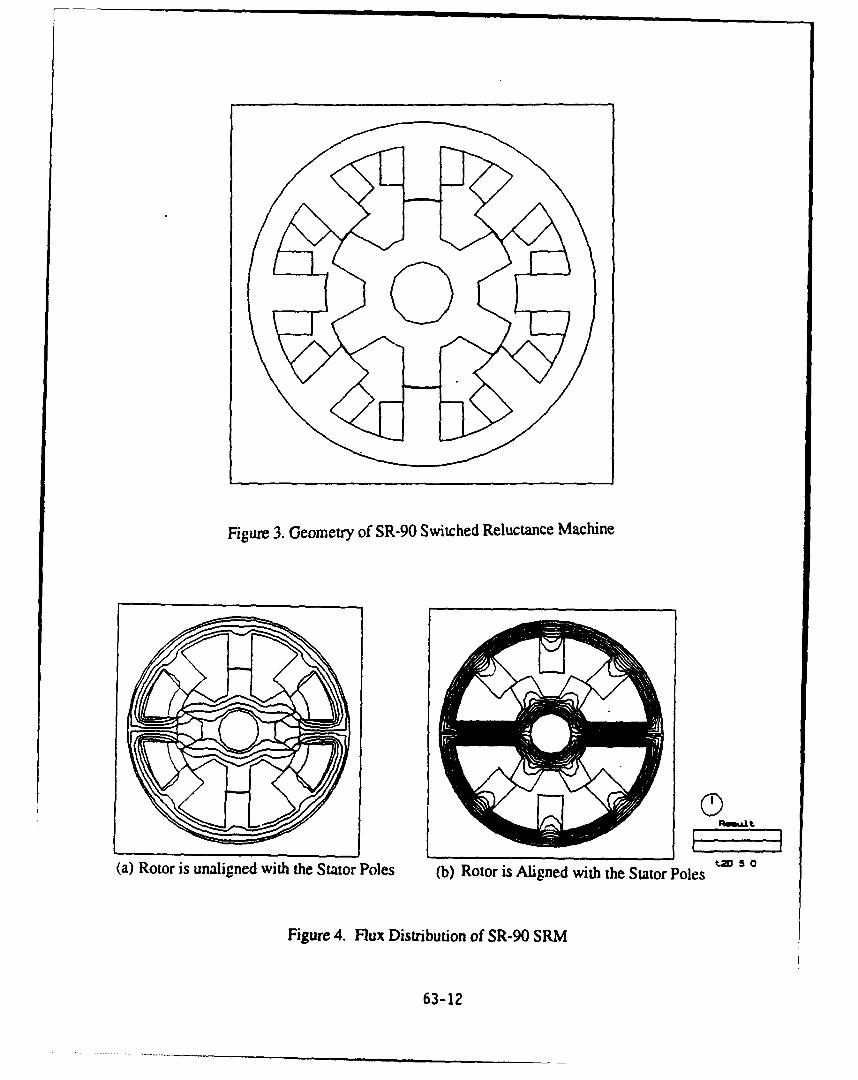
Figure 3. Geometry of SR-90 Switched Reluctance Machine
(a) Rotor is unaligned with the Stator Poles (b) Rotor is Aligned with the Stator Poles
Figure 4. Flux Distribution of SR-90 SRM
63-12

4.2 Winding Flux Linkages
As far as the terminal characteristics of an electric machine is concerned.
computation of winding flux linkages provides a solution. Flux linkages are calculated
because variations of flux linkages due to the mechanical movement determines the induced
speed EMF, the kernel of electromechanical energy conversion. In equivalent circuit
analysis, flux linkages are modeled by the product of inductance and current. However,many researchers have noted that inductance representation does not adequately account for
local saturation or the non-linearity of magnetic field in the machine. If the flux linkageswere modeled directly, and highly accurate model would result. This direct modeling of
flux linkage could be done using finite element analysis.
Winding flux linkages have been computed for the SR-90 machine in this research
project at many current levels for many rotor positions. The results are shown in Fig. 5.
As clearly indicated by the computer results, the flux linkages are functions of both rotor
positions and current levels. In particular, the relations between the current and flux arehighly nonlinear and the non-linearity is further complicated by different rotor positions.
When the rotor is near the unaligned position with respect to the stator pole, flux linkage is
almost a linear function of current and insensitive to the rotor positions. As soon as the
rotor pole reaches positions close to the stator pole, magnetic field saturates and the
influence of the rotor position becomes obvious, indicated by the distance between the flux
linkage lines in the same figure.
The flux linkage profile described by the figure can be used to explain theinadequacy of SRM equivalent circuit where the complicated SRM is simply represented by
lumped resistance or inductance parameters. Compared with the equivalent circuit, the
computed flux linkages by FEM give much better results for SRM modeling. For a given
SRM the flux linkages can be computed or measured comprehensively to encompass all the
possible operating points and then the data can be stored in a look-up table. During systemsimulation, the look-up table is repetitively accessed to search for the actual operating point.
Nevertheless, in certain situations, computing and storing a large number of datafor winding flux linkages have difficulties which, to a certain extent, restrict the use of the
method. For example to model multiphase excitation with winding mutual coupling, twoor more phases of winding currents are considered. The possible combinations of the
63-13

current levels from different phases are vast. To evaluate every possible current
combination under many rotor positions, the computation time and storage memories maynot be practical, if not impossible. Other limitations of the method include the lack of
description of the internal magnetic field and the accuracy problems caused by interpolation
of an actual operating point based on finite computed or measured operation points.
0.20
0.16
0.12-
004"
0.00-11Excitation lamps)
0.00*
0.0 0.5 1.0 1.5 2.0 2.5 3.0
Figure 5. Plot of Flux Linkages of the SR-90 SRM
63-14

4.3 Simultaneous Field and Circuit Analysis
From the results and discussions presented above, it is made evident that
simultaneous computation on the magnetic field and system circuit is attractive and, in some
cases, necessary. The method is especially suitable for investigating dynamic behavior of
the SRM in which both the terminal characteristics and corresponding internal magnetic
field are concerned. The SR-90 machine is analyzed by the coupled field and circuit
modeling method with the operating conditions summarized in Table 2.
TABLE 2
rotor speed 5000 rpm transistor turn-on angle 300DC bus voltage 160 volts transistor turn-off angle 45°
Fig. 6 shows the internal flux distribution of SR-90 covering 30* rotation of the
rotor in 3* steps. It is interesting to notice that the flux density in general increases over the
entire cross-section of the SRM in time. However, the corner tips of both rotor and stator
poles saturate more quickly when the rotor moves towards the alignment with the stator.
This local saturation reduces later when the rotor moves further towards the stator poles.
The SRM magnetic field is fully charged in 15" of rotor rotation and gradually discharged
to zero at approximately another 150 rotor rotation. From the dynamic plot of the SRM flux
distribution, other important variables, such as the torque. radial forces can be conveniently
evaluated in the post process.
As stated previously, the coupled field and circuit modeling method not only reveals
the internal magnetic field variation, but also gives the description of terminal characteristics
on the SRM for the same instants. Fig. 7 shows the current and imposed voltage at the
terminal of the winding while the SRM experiences a series of flux changes plotted in Fig.
6. Note that although the input voltage maintained constant, the phase current fluctuates
around 1.65 amps after the current reached its peak value at about 8* rotor rotation.
Furthermore, the peak current is not corresponding to the instant when the maximum flux
linkage occurs.
63-15

I/i
Fiur 6 lu DstiutonCoeing3°R
to<oaio ihV ltg-orc
oto
631
II! ~ ~< 7*llIIIII

5. Results of Experimental Testing
For the same operational conditions as simulated in the last section, the SR-90machine is tested in the laboratory. The SR-90 is mechanically coupled to a dynamometer
as the load. During testing, the tested machine delivers 30 oz-in torque. Fig. 8 shows theoscillagram traces of the phase current. Compared to the tested results, the currentwaveform predicted by the coupled field and circuit modeling method is in very good
agreement with that from the testing. The accuracy of the modeling method is verified.
20
+ fo -,-
0.0 124 30 36 42 4A 54 60
Rotor angle (degs)
Figure 7. Predicted Current Waveform from Modeling
61
K.... .... ,,
Cr1 10 OmVO M 200Ms Chi J
Figure 8. Measured Current Waveform from Testing
63-17

6. Conclusions and Future Work
Modeling of the SRM system is very complicated. The complicity stems from the
highly nonlinear nature of the magnetic field and its interaction with the unconventional,
electronic control of the SRM system. To fully account for the complexity, a simultaneous
modeling of the SRM internal magnetic field and external power electronics circuitry is
necessary. The coupled field and circuit modeling technique presented and implemented in
this research work provides a powerful tool for the situation. Through principle
discussion, modeling development, computer implementation, and experimental validation,
the following conclusions have been reached.
1). The conventional magnetostatic finite element analysis can be extended to include
circuit analysis to investigate complicated transient behavior of SRM systems. Formulation
of the problem is simple and conveys very understandable physics of the modeled system.The implementation of the modeling can be realized conveniently by using commercially
available and technically matured finite element packages used for static field analysis. The
programming time and cost for modeling is minimum, and the accuracy is high.
2). The outputs from the combined field-circuit modeling method are comprehensive. In
the field-circuit coupled approach, investigation is conducted in time domain. Therefore,
the solutions to the field equations naturally presents the results of the field variation both in
space and in time, as opposed to the those obtained from conventional static field analysis.
Furthermore, the modeling method enables the circuit current to interact with the field flux
intensively under the constrains imposed simultaneously by the voltage and field equations.
The results, therefore, contains all information regarding the effects of interaction between
the external circuit and internal magnetic field.
3). The coupled field-circuit modeling is versatile and flexible. In the field-circuit
modeling of the SRM, the inputs to the system are the terminal voltages to the windings,
rather than current, and the geometry and material specifications of the SRM. Both the
input functions and the geometry specifications of the SRM can be changed flexibly
according to the modeling purpose. By changing the input voltages, various electrical fault
conditions can be simulated. In other situations, we can change the geometry or material of
the SRM to model mechanical or material errors. Regardless of the origins of the fault or
error (electrical or mechanical, internal or external), the results from the modeling will be
63-18

EFFECT OF FREE STREAM TURBULENCE ON THE BURST
PHENOMENA AT THE WALL IN A WALL-JET
SAVAS YAVUZKURT
Associate Professor
Department of Mechanical Engineering
The Pennsylvania State University
University Park, PA 16802
Final Report for
Summer Faculty Research Program 1993
WLIPO Wright Patterson AFB, Ohio
Sponsored by
Air Force Office of Scientific Research
Boiling AFB, Washington, DC
and
WL/POTC Aero Propulsion & Power Directorate
September 1993
64-1

EFFECT OF FREE STREAM TURBULENCE ON THE BURSTPHENOMENA AT THE WALL IN A WALL-JET
SAVAS YAVUZKURTAssociate Professor
Department of Mechanical EngineeringThe Pennsylvania State University
University Park, PA 16802
Abstract
Effects of free stream turbulence (FST) on the burst phenomena at the wall was studied
in a wall-jet flow. It was found that the number of bursts and/or ejections associated with a
burst event per unit time increases with increasing intensity of FST. This fact can be used as an
explanation of why FST results in an increase in the heat transfer at the wall. For this purpose
a wall-jet test rig was designed and built. The initial height and velocity of the jet were 4" and
73.5 ft./s respectively. The ejection processes associated with a burst event were identified
from the output of a surface flush hot-film probe positioned at 4" intervals on the surface along
the flow direction. The profiles of mean velocity, axial component of the turbulent stress were
measured with a horizontal hot-wire probe. Autocorrelations were used to calculate the length
scales in the flow direction. Two horizontal hot-wire probes were used for the measurement of
length scales in the spanwise and vertical directions. Large amounts of data were collected.
Apart from the important result of increase in the rate of ejections with increasing FST
intensity, further analysis of data is expected to reveal some of tha fundamental mechanisms
through which FST affects the rate of heat transfer.
64-2

EFFECT OF FREE STREAM TURBULENCE ON THE BURSTPHENOMENA AT THE WALL IN A WALL-JET
SAVAS YAVUZKURT
Free-stream turbulence (FST) is the turbulence in the approach stream. It is
experienced in many applications. For example, nozzle guide vanes and rotor blades in a gas
turbine are exposed to high levels of FST.
The FST has an important influence on the heat transfer. Under high levels of turbulence
(10-20%) there is an appreciable increase in the heat transfer rate regardless of the
character of the boundary layer.
Some representative results in this area can be found in the studies by Kestin (1 966),
Kearney et al. (1970), Brown and Burton (1978), Bradshaw and Simonich (1978), and Blair
(1983). A detailed review of this literature is given by Moffat and Maciejewski (1984). They
conclude that the free stream turbulence levels up to 10% cause a proportional increase in heat
transfer for constant velocity and accelerating turbulent boundary layers. It is indicated that
large effects on the average values may result if the turbulence affects the location of the
transition and if the heat transfer data are compared at constant x-Reynolds numbers.
One of the important observations from the literature in this area is that, under the
same levels of turbulence, different researchers have found different enhancement of heat
transfer rates. This leads to the speculation that not only the velocity scale but also the length
scale of the turbulence is important. In fact, Moffat and Maciejewski (1984) relate to this fact
and suggest that the effect of the length scale should be investigated.
Most of the studies that were discussed used, one way or another, grid generated
turbulence in their experiments where the length and velocity scales are usually small. More
recently, the flow fields of jets and wall jets have been used in order to simulate high free
stream turbulence encountered in turbomachinery. Moffat and Maciejewski (1985) used a
circular wall jet in order to obtain free stream turbulence intensities up to 48%. They
measured Stanton numbers which are as much as 350% above the standard zero free stream
velocity gradient turbulence correlations. Ames and Moffat (1990) have investigated the
effects of free stream turbulence created by 2.5 inch diameter jet injection into a main flow in
a plenum chamber followed by a wind tunnel test section on the heat transfer to a flat plate
boundary layer. This study used autocorrelations to measure the length scales. In another
recent study, MacMullin et al. (1989) investigated the effects of free stream turbulence from a
circular wall jet on a flat plate boundary layer heat and momentum transfer with turbulence
64-3

intensities 7-18%. They also observed increased Stanton numbers and skin friction coefficient
with increasing turbulence intensities. They used autocorrelations for the determination of
length scales. The influence of length scale on the Stanton numbers was not conclusive. Rivir et
al. (1992) studied the heat transfer in a 20 planar wall jet up to FST intensities of 20% and
observed up to 100% increases in heat transfer compared to standard correlations. However,
no general correlation could be found that would represent the data from all these studies.
The present belief of the author is that the length scales in the vertical direction to the
wall and in the transverse direction to the flow are more important in determining the scales
within the boundary layer which affect the heat transfer. Yavuzkurt ý 1990, 1993) has
carried out experiments on the experimental set up used by Ames and Moffat (1990). In these
experiments length scales of all the turbulent stresses were measured in all three coordinate
directions both in the free stream and within the boundary layer using two triple hot wire
probes. A quantity FST number was defined using all the velocity and length scales of the normal
stresses in the free stream normalized by the boundary layer thickness and free stream
velocity. This quantity correlated the heat transfer data very well.
A detailed discussion on the free stream turbulence distortion for flows approaching
stagnation and its effects on heat transfer can be found in Yavuzkurt and Tafti (1987) and Tafti
(1989). It was seen from these investigations that there is a need to understand the
fundamental mechanisms through which FST effects heat transfer. A fundamental study of near
wall layers of the flow under the effects of FST might be helpful in clarifying these issues.
Research on structure of turbulent flows have shown that they contain considerable
structure. The presence of near wall "streaks" and "bursts" are well documented. These are the
structures that are found in the viscous sublayer and that differentiates turbulent flows from
laminar flows. One means of investigating the flow structures is called "quadrant analysis"
(Wallace et al. 1972, Willmarth and Lu, 1972). The technique involves partitioning the flow
signal into four quadrants based on the instantaneous signs of the fluctuating velocity
components u' and v'. As explained in Volino and Simon (1993), in a boundary layer type flow
when the wall is heated, a turbulent parcel of fluid moving away from the wall (v'>O) would
most likely to be of relatively low velocity (u'<O) and high temperature (t'>0). Such a motion
would be classified as a "hot ejection". The present author's opinion is that this hot ejection is
related to the burst phenomena and will increase the heat transfer at the wall. Therefore, there
is a strong correlation between the instantaneous increase in heat transfer and ejections. It is
postulated that FST leads to increases in burst events at the wall thereby increasing the heat
transfer. The main objective of this research is to test this hypothesis.
64-4
ExIerimental Procedures
The experiments were carried out in a wall-jet flow as shown in Figure 1. The rationale
in using wall-jet flows for simulating high FST is explained in Moffat and Maciejewski
(1989), MacMullin et al. (1989) and River et al. (1992). A centrifugal blower with a flow
rate 2000 scfm is connected to a transition section containing a honeycomb. Honeycomb was
used to even out the disturbances in the blower flow. A sheet metal nozzle was built with an exit
which was 4" high and 1 ft wide giving it an aspect ratio of 3. The initial jet velocity at the
centerline was about 80 ft./s. To the nozzle exit a test section made of plexiglas was attached.
The test surface was 6 ft. long and 1 ft. wide. The side walls were 1 ft. in height in order to
prevent external disturbances. The top of the test section was open to facilitate a wall-jet flow.
However, a top wall was also built to be used later for boundary layer type flows.
The velocity data was taken with two TSI 1210-T1 .5 horizontal hot wire probes. A
universal traverse mechanism was built which allowed the probes to be moved in "y" (vertical)
and "z" (transverse) directions with respect to each other for space correlation measurements.
The probes can also be moved in "x" (axial) direction with a slider mechanism riding on the side
wall of the test section. A TSI 1237 surface flush hot film probe was used to measure
instantaneous heat transfer thereby to identify the ejections of turbulent fluid from the wall.
Test surface had 1/2" holes located at 4" centers for the positioning of the plug that held the hot
film probe. The hot wire and hot film probes were connected to a TSI IFA 100 flow analyzer
operating in constant temperature anemometry mode. The hot-wire probes were calibrated
using a 486 computer and a calibration program utilizing modified King's Law. The same
computer was also used for data acquisition and partial data reduction. A DT2829, 8 channel
simultaneous A/D board with 30 kHz response for each channel is used as an interface between
the analog signals and the computer. The 486 computer produced instantaneous values of
streamwise velocity u' for both hot-wire probes and also a value proportional to q'
(instantaneous heat transfer) for the hot film probe. These quantities were stored in magnetic
disks and later were analyzed in a main frame computer to produce, mean velocities, rms valuesof u', autocorrelations of u' and q', space correlations of u; and uz (subscripts 1 and 2 refer to
the two hot wire probes) in y and z directions, and space correlations of u; and q' in the y
direction. The correlations were defined as follows:
Autocorrelation of u' R = u' (x, y, z, t)u' (x, y, z, t + At)U6 (x, y, Z, tu 5x, y, Z, t)
64-5

Space correlation of u; and uR = u Z(x' ' t)u;((X, Y +&y Z, t)u'z x,y,Zi~z, xy,zt
in the y direction
Space correlation of u; and uu Ruu = U2 (X, y, z, t)U1 (x, y, z + Az, t)U2 (X, y, z, t)U2 (X, y, z, t)
in the z direction
Space correlation of u' and q' Ruq =I Ay, 0, t=q (x, 0, 0, t)
in the y direction
The data was taken at 4000 Hz with a sample size of 40960 points resulting in 10.2 seconds of
real time data for all quantities measured at every measurement location. The measurements
were made under isothermal conditions.
Results and Discussion
As stated in the objectives at the end of the introduction section, the main goal was to
show that the number of bursts, or ejections related to a burst event increases as the FST
increases. This goal was partly achieved. Figure 2 shows the axial Reynolds stress normalized
by maximum value of the mean velocity at the y location at which the maximum mean velocity
occurs as a function of number of peaks per unit time in the instantaneous heat transfer traces
obtained from the hot film probe. The peaks in the instantaneous q traces will be discussed
later. This figure shows that as hypothesized there is a definite increase in the number of peaks
with increasing FST level.
Figures 3 and 4 show important mean parameters of the wall jet. As expected, the
maximum mean velocity decreases linearly and the Ymax (location at which the maximum mean
velocity occurs) increases linearly in the axial direction. The axial distance was measured
from the end of the nozzle or the start of the test section. These figures indicate the presence of
a well-behaved wall jet.
Figure 5 shows instantaneous traces of q' at the wall (y - 0) indicated by the hot-film
probe as a function of time. The values of q' were normalized with the mean value of the heat
transfer Q. The traces are shown at two axial stations of 4" and 56" along the centerline (z - 0)
64-6

of the test surface. As can be seen, there are definite peaks in heat transfer traces. These peaks
were identified as ejections that are associated with a burst event following Clark et al. (1992)
and Volina and Simon (1993). In calculating number of peaks per unit time the signals were
conditioned in order to reduce the uncertainty such that values of q'/Q<0.02 were discarded.
Then number of peaks per second were calculated for time intervals of 1 s, 2s, 3s, up to 1 Os. It
was seen that in all axial locations number of peaks per unit time reached a steady level within a
1Os time interval. Similar results are obtained if the signal is conditioned such that values of
q'/Q<0.01 are rejected but number of peaks considered increases accordingly.
Figure 6 shows the normalized mean velocity profiles at six axial stations along the
centerline. After some initial nonuniformities the profiles take a well known shape for a wall
jet and the maximum in the mean velocity near the wall starts becoming noticeable at x = 32".
Figure 7 shows the normalized turbulence intensity profiles at six axial stations along
the centerline. The turbulence intensity far away from the wall at about y = 100 mm is high
due to very low levels of mean velocity in these regions. However, the intensity which is
defined as the intensity of FST at y = Ymax increases from 5% to 18% from x = 16" to x = 64".
This is the intensity which is used in calculations for Figure 2. In fact at the last axial station
of x = 64" intensity is almost constant in the y direction.
Figure 8 shows the autocorrelations of u' at different axial locations and at y = yrnax-
There is a definite increase in the integral timescale after the shear layer of the wall jet is
established. These time scales when multiplied with the mean velocity at y = Ymax results in
the length scales in the axial direction.
Figure 9 gives the space correlation of u' and q' at several axial locations. As can be seen
from this figure the values of Ruq near y = 0 are quite high, they are in the order of 0.6 in the
developed wall jet. Considering in the definition of Ruq the denominator is -u' . q , this high
value indicates a very strong correlation between u' and q' as expected. It is also apparent from
this figure that the effects of fluctuations far from the wall (y - 60 mm for a 100 mm initial
wall jet height) is felt at the wall, indicating high levels of FST strongly influences the events
near the wall.
Figure 10 shows the autocorrelations of q' at several axial locations. Again, the time
scales of q' fluctuations increase in the axial direction. Considering that the eddies containing
this energy traveling with the speed of the flow near the wall, a length scale for q' eddies or a
size for the region of effect can be defined.
A video containing quadrant plots ofu' , u' and q' has also been made and it is available
from the author.
The space correlation coefficients betweenu; and uý in the y direction at y = Ymax is
shown in Figure 11 at several x locations. As can be seen all the length scales in the vertical
64-7

direction in the developed wall jet (after x - 32") are about 80 mm long (if extrapolated).
This indicates a strong interaction between the outer and inner layers of the flow. In fact, at
x = 16" there seems to be a dual length scale. One for the free shear layer and the other for the
injected wall jet.The space correlation coefficients in the z direction for u' and u' can be seen in Figure
12 at several locations along the centerline. It looks like length scales in z direction are also
quite long especially in the near jet up to x = 32". However, at stations x = 48" and 64" they
are very similar to y scales and are about 80 mm long. Again the dual length scale structure can
be seen at x = 4" and 16".
Figure 13 shows the length scales (Lux, Luy, Luz) of u' in x, y, and z directions. These
length scales were obtained at a location where the value of the correlation coefficient is Ruu =
0.5 due to the limits of the data. There seems to be a decrease in the length scales in the y and z
direction for the near jet up to about 48". This is the region in which dual length scale
structures are obtained. Whereas the length scale in the x direction stays pretty much constant.
For the established wall jet however, the length scales in the x and y direction increases in the
axial direction and the length scale in the z direction stays pretty much constant. Effect of these
length scales on the burst phenomena will be analyzed later.
Conclusions
"* Experiments were carried out in a wall jet to explore the effects of high FST on the
burst phenomena at the wall.
"* It was found that number of ejections identified by the number of peaks in the
instantaneous q' traces increases as the FST intensity increases as postulated.
"* Length scales of u' were measured in all three coordinate directions using auto and
space correlations. These length scales are quite long (- 80 mm) when compared to
initial thickness of the jet and indicates strong interaction between outer and inner
layers of the flow. Effect of these scales on burst phenomena will be analyzed later.
"* Space correlations between u' and q' in the vertical direction show that the effects of
fluctuations as far as 60 mm from the wall are felt at the wall suggesting
mechanisms through which FST affects heat transfer.
64-8

FutureWorkThe work here is by no means complete. The large amount of data stored in disks will be
analyzed further in order to explore the relationship between the length scales of FST and the
burst phenomena. The same experiments will be repeated using two triple wire probes for the
measurement of length scales of u', v' and w' components in all three coordinate directions. It is
possible that v' and w' components of FST have more important effects on the events near the
wall. VITA techniques such as explained in Bogard and Tiederman (1986) will also be used to
identify the burst events. Results of this technique will be compared with the results obtained
from the peak counting technique used here. A proposal to carry out this work will be submitted
to AFOSR Summer Research Extension Program.
Acknowledgmens
Author expresses his deep appreciation to AFOSR Summer Faculty Research Program for
supplying this opportunity to carry out this research at WPAFB. His sincere thanks goes to Dr.
Richard Rivir of WL/POTC, WPAFB for his help and guidance during this research. The last but
not least, the cooperation of Greg Cala, David Pestian and John Schmoll are greatly appreciated;
their help made it possible to get so many results in a two month period.
References
Ames, F. & Moffat, R. J. 1990. Heat Transfer with High Intensity, Large Scale Turbulence: The
Flat Plate Turbulent Boundary Layer and the Cylindrical Stagnation Point. Rep. No.: HMT-44
Thermosciences Div. Mech. Engr. Dept., Stanford University.
Blair, M. F. 1983. Influence of Free Stream Turbulence on Turbulent Boundary Layer Heat
Transfer-Part I and II. ASME J. of Heat Transfer, February.
Bogard, D. G. & Tiederman, W. G. 1986. Burst Detection with Single-Point Velocity
Measurements. J. Fluid Mech., Vol. 169, pp. 389-413.
Bradshaw, P., & Simonich, P. 1978. Effect of Free Stream Turbulence on Heat Transfer
Through a Turbulent Boundary Layer. ASME J. of Heat Transfer, 100-4.
Brown, A., & Burton, R. C. 1978. The Effects of Free Stream Turbulence Intensity and Velocity
Distribution on Heat Transfer to Curved Surfaces. J. of Engr. for Power, 100, 159-168.
64-9

Clark, J. P., LaGraff, J. E., Magari, P. J. & Jones, T. V. 1992. Measurement of Turbulent Spots
and Intermittency Modelling at Gas Turbine Conditions. Proc. of the 80th Symp. of
NATO/AGARD, Propulsion and Energetics Panel. Heat Transfer and Cooling in Gas Turbines.
Antalya, Turkey, 12-16 Oct. 1992.
Kearney, D. W., Kays, W. M., & Moffat, R. J. 1970. The Effect of Free Stream Turbulence on
Heat Transfer to a Strongly Accelerated Turbulent Boundary Layer. Proc. of 1970 Heat
Transfer and Fluid Mechanics Institute, edited by T. Sarpkaya.
Kestin, J. 1966. The Effect of Free Stream Turbulence on Heat Transfer Rates. Advances in
Heat Transfer.
MacMullin, R., Elrod, W., & Rivir, R. 1989. Free Stream Turbulence from a Circular Wall Jet
on a Flat Plate Heat Transfer and Boundary Layer flow. Trans. ASME J. of Turbomachinery, iii,
78-86.
Moffat, R. J., & Maciejewski, P. K. 1984. Effects of Very High Turbulence on Convective Heat
Transfer. Proc. of HOST Conference, NASA Conference Publication 2339, NASA Lerc, 381-388.
Moffat, R. J., & Maciejewski, P. K. 1985. Heat Transfer with Very High Free Stream
Turbulence. Proc. of HOST Conference, HASA Conference Publication 2405, NASA Lerc, 203-
215.
Rivir, R. B., Troha, W. T., Eckele, W. A., & Schmoll, W. J. 1992. Heat Transfer in High
Turbulence Flows-A 2D Planar Wall Jet. Proc. NATO/AGARD 80th Symposium of the
Propulsion and Energetics Panel, Antalya, Turkey, 12-16 October 1992.
Tafti, D., 1989. Prediction of Heat Transfer Characteristics for Discrete Hole Film Cooling on
Flat Plate and Turbine Blades. Ph.D. Dissertation, Penn State Univ., Dept. of Mechanical Engr.
Volino, R. J. & Simon, T. W. 1993. An Application of Octant Analysis to Turbulent and
Transitional Flow Data. ASME Paper #93-GT-72. Presented at the Intl. Gas Turbine and
Aeroengine Congress and Exposition, Cincinati, OH, May 24-27, 1993.
Wallace, J. M., Eckelmann, H. & Brodkey, R. S., 1972. The Wall Region in Turbulent Shear
Flow. J. Fluid Mech., Vol. 54, Part 1, pp. 39-48.
64-10

Willmarth, W. W. & Lu, S. S. 1972. Structure of the Reynolds Stress Near the Wall. J. Fluid
Mech., Vol. 55, Part 1, pp. 65-92.
Yavuzkurt, S., & Tafti, D. 1987. Turbulence Modeling for Flat Plate and Turbine Airfoil with
Discrete Film Cooling. Contractors Report RFQ:PC693359, Textron Lycoming Corp., Stratford,
Conn.
Yavuzkurt, S. 1990. Characterization of Length and Velocity Scales of Free Stream Turbulence
and Investigation of their Effects on Surface Heat Transfer. Center for Turbulence Research,
Stanford University, Annual Research Briefs 1990, pp. 253-262.
Yavuzkurt, S. & Batchelder 1993. A Correlation for Heat Transfer under High Free Stream
Turbulence Conditions. Proc. of 9th Symposium on Turbulent Shear Flows, Kyoto, Japan, Aug.
10-18, 1993.
1' IHOT WIRE PROBES HOECM
12"L.__ .WALL J. 4'x "72-' ISURFACE FILM PROBE BLOWER
S~IFA 100
AD ANEMOMETER
IT OUTPUTS486 COMPUTER u', q' FILES
FIGURE 1. WALL JET TEST RIG AND DATA ACQUISITION SYSTEM
64-1 1

C)
00
0 0
-W-
x LA
'~ -, mot',
0~~~~~~ a)______ 4
C 0 0
o to r4~).uf
0
0 c
_u 0
0 V0z- LL
0 _
co o .4
o 0z
-o-
0
oD 04 0a C0L 0 0to ' 0 Lo 0o (
c' 5 - 0 0 0 Jj-w
x~uwf/luAin U.-
COPY AVAILABLETOCQ.'-- TO 4-p..-..-..
64-12

-- -- 150RUN N0:616UP11 -16 x=0- z-o" U..,-7.-5 ft/s RUNN0:616UP1
7-2? x-4- z--0 U.,.'.7..5ft/s
120
90
E60
30
0
0.0 0.2 0.4 0.6 0.8 1 .0 1.2 0.0 0.2 0.4 0.6 0.. 1 .0 1.2U/Umo,. U/U,.•.
'U1 x-16" z O • ' t150..
RUN N0:61 6UP01 -1 0 s- 6" z=O'" U,.,=.-72 ft/s RUN NO:616UP26-35 x-32" zO=" U,,.,=70.5 ft/s
1 120
90
60
30 .
S S
0.0 0.2 0.4 0.6 0.5 1.0 1 .2 0 .
U/Urn° 0.0 0.2 0.4 0.6 0.8 1.0 1.2
* .150 ,
RUN NO:621UPO -. 10 x=48- z=0- U,,.=68 ft/s RUN NO:621 UPI 1-20 x-64" z=0" U,.•59.4 ft/i
120
* 90E
* 60-
U/Urn0I *° . , 0 . U/U. , I •.
0.0 0.2 0.4 0.6 0.8 1.0 1.2 0.0 0.2 0.4 0.6 0.8 1.0 1.2u/u,,,• U/Urno,
FIGURE 6. MEAN VELOCITY. PROFILES IN THE WALL JET RIG
COPY AVALR ABLE TO E L'lC - .'-'- , .... .- .I - " .
64-13

0- '205. ,
0 9c I E
E 0
50 o 60
3 0 x 0 -ý -- 0 - U rnm '3 .5 f t / s I30 30 x=4" z=O" fc=7 3 .S ft/s
_ _ _ _ _ _ _ _ _ I °
0 0 ' 9 o0.00 1.05 0.10 0.15 02C 0.25 0.00 0-05 0.10 cl 5 0.20 0.25
Um,/UmO. u,m,/u,,,o.
50 1500
20 0 120 x=32" z=O" Umox=70 ft/sx='" z=C" Umo,=72 ft/s
0goo
90 E,,90
E 00 E
60 0 00
30 300
0 00 %,Cb" 0 (, 0- .
0.00 C.05 0.10 0.15 0.20 0.25 0.00 0.05 0.10 0.1 5 0.20 0.25urms/Uma. u,,ms/u,,•.
____ ___ ___ ____ ___ ___ ____ ___ ___ ____ ___ ___ 1 505000 I
0 J 12 0
20 x=64" z=O' Uox¼SC.4 f'/x=48"' z=O" Umox=68 ft/s 0./s
0
. , 90-90 E 0a E
60 0 60 0
60 00
30 0 30 0
0 00 0
0 0.000.050.10 0.15 ,0. 0 02 ,
0.00 0.05 DAD 0.15 0.20 0.25urms/Uma,
FIGURE 7. TURBULENCE INTENSITY IN THE WALL JET RIG
64-14

10
S0.8
RUN NO 623UUEI O5.COR x=4"y=i5mmz=0 RUNNO623UUE]1.COR x=16"y=2OrnzwO'
-• 0.4
0.010 0.02 0.04 0.06 0.08 0.10 0.00 0.02 0.04 0.06 0.08 0.10Ar~s) at(s)
1.0
0.3
RUN NO 623UUE30.COR x=32" y=2 5 mm z=0" 0.6 RUN NO 624UUE1I0.COR x=48" y=25 mm z=O"
0.4
,- 0 , ... .0 - ...0.02 0.04 0.06 0.08 0.10 0.00 0.02 0.04 0,05 0.08 0.10wt(s) At(s)
1.0
0.8
0.6 RUN NO 624UUE20.COR x=64" y=50mm z=O*'
0.4
0.2
0.00.00 0.02 0.04 0.06 0.08 0.10
dt(s)
FIGURE 8. AUTOCORRELATION OF u' IN THE WALL JET RIG
COnAVAILABLE TO DTC0-L"•".,64-,64-'15
,0 1 1.0
-RUN NO:16UP01 -110 x= 6- z=O" .6 RUN NO:61 6UP26-35 x= 32- z=0-6~~~~ ~~ RUN:=6O"-~x.'z
),40.
)2 0.2
. p 0.00 30 60 90 120 150 0 30 60 90 120 150y(mm") y(mm)
1.0
0.8;
'RUN NO:621 UP01 -1 0 x= 48" z=0" 0.6 \ RUN NO:621 UP1 -20 x= 64" z=O"
0.4
2 ~0.2
0 0.0.0 30 60 90 120 150 0 30 60 90 120 150
y(mmn) y(mn-,)
FIGURE 9. SPACE CORRELATION OF u' AND q' IN THE WALL JET RIG
64-16

1 .0
- 0.8
RUN NO623UUE05.COR x4y=OmmZO 0.6 RUN NO 623UUE11 .COR x-1 6" y-O rn zO0"
0 0 0.. 00.0.00 0.02 0.04 0.06 0.08 0.10 0.00 0.02 0.04 0.06 0.08 0.10
0.8\ RUN NO 623UUE30.COR x=32"y=Ommz=0" 0.6 RUN NO 624UUEIO.COR x-48"y=OmmZ=O"
0.4
J 0.2
0.0
.00 0.02 0.04 0.06 0.08 0.10 0.00 0.02 0.04 0.06 0.08 0.10At(s) At(s)
"..0
0.8
0.6 RUN NO 624UUE20.COR x=64" y=O mm Z=O'
0.4'
RNN62
0.2
0.00.00 0.02 0.04 0.06 0.08 0.10
A.l(s)
FIGURE 10. AUTOCORRELATION OF q' IN THE WALL JET RIG
COP'Y AVAILaIL TO-. ,-'.--
64-17

o 1.0 -RUNNO: 622UUE01-04 x'=0"z20- y2=5Omm 0 RUNNO: 623UUE01-05 x=4" z=O0 y2l 5 mm8 -I 0.8 ,
6 0.6
40.4
2 0.2
0 " ' ' ' '0.00 20 40 60 s0 100 0 20 40. 60 80 1 00Ay(mm) Ay(mfl'l
UN NO 62UE 61.0l6'=" 22 mRNN: 2UE1-5x32 "Y=5m
RUN NO: 623UUE1 6-20 x=-6z=0" y2=20mm , NO. 623UUE21 -25 -=32" z=0" y2=25 mmS~~0.86 'O
0.6
0.4
0.2
I ,0.00 20 40 60 50 00 0 20 40 60 80 100
,y(mm) ay(mm)
'1.
i RUN NO: 624UUE06-1 0 x=43" z=0" Y2= 2 5 mm RUN NO: 624UUE1 1 -15 x=6 4 " z=0" y2= 5 0 mm
80.5
,60.
4 0.4
.2 0.23
.0 0.00 20 40 60 80 100 u 20 40 60 80 100
FIGURE 11. SPACE CORRELATION OF u'1 AND U'2LENGTH SCALE MEASUREMENT AT Umax LOCTON
COPY AVAAL 64-18
1 1.0 ,
NO 622UUE05-09 x=0 z=O" y,. 5 0 mm I RUN NO: 623UUE06-10 x=4'Z=0" y2,=l5nnm
0.8
0.6
0.4
0.2
D0.0 -1
o 20 40 60 80 100 0 20 40 60 80 100Az(mm) &z(mm)
UN N 623UUE1 -15 x=1 6" Z=0" Y m=20 -m RUN NO: 623UUE26-30 x=32" z=O" Y2= 2 5 mm0.8
0.6
4 0.4
2 0.2
0 1 0.0Ozm 20 40 60 80 100 0 20 40 zcmm) 60 80 100
1.0
RUN O:64UU01-5 x4'2= y 2 5mmRUN NO: 624UUEI 6-20 x= 6 4 " z-=0 Y2= 5 0 mmrRUN NO: 624UUE01 -05 x=48" z=0" Y2=25 MM i 0.
J 0.6
0.4
2 0.2
0.0 1' '
0 0 20 40 60 80 100
0 20 40 60 so 0C az(MM.)
FIGURE 12. SPACE CORRELATION OF u'l AND U'2LENGTH SCALE MEASUREMENT AT Umax LOCATION
COPY hVAILABLL ± ii oC ~±±~-. ~- .
64-.19
iL ..--

120
00
soE •• Luy I
S60 Lu
0_ 40 •
20 S
0 1S I *
0 20 40 60 80 1O0
x(in)
FIGURE 13. LENGTH SCALES OF u' OBTAINED FROM THE RuuAT A LOCATION WHERE Ruu = 0.5
64-20