Wind driven currents in the

. . . . . . . . . . . . . . . .

. . . . . . . . . . . . . . . .

. . . . . . . . . . . . . . . .

. . . . . . . . . . . . . . . .

. . . . . . . . . . . . . . . .

. . . . . . . . . . . . . . . .

. . . . . . . . . . . . . . . .

. . . . . . . . . . . . . . . .

. . . . . . . . . . . . . . . .

. . . . . . . . . . . . . . . .

. . . . . . . . . . . . . . . .

. . . . . . . . . . . . . . . .

. . . . . . . . . . . . . . . .

. . . . . . . . . . . . . . . .

. . . . . . . . . . . . . . . .

. . . . . . . . . . . . . . . .

. . . . . . . . . . . . . . . .

. . . . . . . . . . . . . . . .

. . . . . . . . . . . . . . . .

. . . . . . . . . . . . . . . .

. . . . . . . . . . . . . . . .

. . . . . . . . . . . . . . . .

. . . . . . . . . . . . . . . .

. . . . . . . . . . . . . . . .

. . . . . . . . . . . . . . . .

. . . . . . . . . . . . . . . .

. . . . . . . . . . . . . . . .

. . . . . . . . . . . . . . . .

. . . . . . . . . . . . . . . .

. . . . . . . . . . . . . . . .

. . . . . . . . . . . . . . . .

. . . . . . . . . . . . . . . .

. . . . . . . . . . . . . . . .

. . . . . . . . . . . . . . . .

. . . . . . . . . . . . . . . .

. . . . . . . . . . . . . . . .PAOLA CASTELLANOS OSSA

Wind driven currents in the coastal and equatorial upwelling regions

Wind driven currents in the coastal and equatorial upwelling regions

La circulación generada por el viento en regiones de afloramiento

costero y ecuatorialMemoria de Tesis doctoral presentada por

PAOLA CASTELLANOS OSSApara optar al grado de Doctor en Ciencias del Mar

Departament d’Enginyeria Hidràulica, Marítima i AmbientalUniversidad Politècnica de Catalunya

Tesis doctoral Dirigida porel Doctor Josep L. Pelegrí

Institut de Ciències del MarCentro Superior de Investigaciones Científicas

Barcelona, a 12 de Noviembre de 2012

Dedicada a mi abuela Clara Rua Ortega

Por sus sólidas enseñansas, y por regalarme desde el amor, bases sólidas donde construir mi propio camino

para ti tatica... esta tesis forma parte de tu legado

Preface / Prefacio ................................................................................................... 6

Abstract / Resumen ....................................................................................................... 8

Chapter 1 Introduction and objectives ....................................................... 14

Chapter 2 Winter and spring surface velocity fields in the Cape Blanc region as deduced with the Maximum Cross-Correlation technique ...................................................... 28

Chapter 3 Wind-driven surface circulation in the Cape Blanc region ............................................................. 52

Chapter 4 Response of the surface tropical Atlantic Ocean to wind forcing .............................................................................. 84

Chapter 5 Conclusions ..................................................................................120

References .........................................................................................................128

Acknowledgements / Agradecimentos ................................................142

Contents

6

Wind-driven currents in the coastal and equatorial upwelling regions

Preface

This dissertation, entitled WIND-DRIVEN CURRENTS IN THE COASTAL AND EQUATORIAL UPWELLING REGIONS, is presented as a partial requirement to obtain the Doctoral degree from the Universitat Politècnica de Catalunya. This investigation is the compilation of three studies aimed at describing the processes generated by the wind in two upwelling regions typical for subtropical and tropical Atlantic. This thesis investigation was conducted between 2009 and 2012 under the guidance of Dr. José Luís Pelegrí Llopart, who is an investigator from the Institut de Ciències del Mar - Consejo Superior de Investigaciones Científicas, mainly in the frame of the research project entitled “Ocean Climate Memory: mechanisms and paths of surface water formation in the Equatorial Atlantic” (MOC2-Ecuatorial, ref. CTM2008-06438-C02-01/MAR).

This doctoral dissertation is structured with an introductory chapter which describes the physical oceanography of upwelling regions in both the coastal and the open oceans and summarizes the principles used throughout the thesis. The following three chapters constitute the core of the dissertation, each of them is presented as a scientific article. While writing this thesis, the first of these articles has been accepted for publication by the International Journal of Remote Sensing. The second article has been submitted to Continental Shelf Research and is currently under revision, and the third article is in the last phases prior to its submission to a scientific journal. The thesis concludes with a discussion of the main results from this work, as well as with comments on potential future lines of research. Asides the above-mentioned articles, along this period of research the author of this thesis has participated in three symposia, has coauthored one research paper published in Scientia Marina, and has been the principal author of one chapter of a proceedings book.

Paola Castellanos Ossa

7

Preface

Prefacio

Esta memoria de tesis, titulada LA CIRCULACION GENERADA POR EL VIENTO EN REGIONES DE AFLORAMIENTO COSTERO Y ECUATORIAL, se presenta como parte de los requisitos para obtener el grado de Doctor por la Universitat Politècnica de Catalunya. El trabajo de investigación es una compilación de tres estudios que buscan describir los procesos generados por el viento en dos regiones de afloramiento características del océano Atlántico Tropical y Subtropical. Dicho trabajo se ha llevado a cabo durante los años 2009 a 2012 bajo la tutela del Dr. José Luís Pelegrí Llopart, investigador del Institut de Ciències del Mar, Consejo Superior de Investigaciones Científicas, fundamentalmente en el marco del proyecto de investigación titulado “Memoria Océanica del Clima: mecanismos y rutas de formación de aguas superficiales en el Atlántico Ecuatorial” (MOC2-Ecuatorial, ref. CTM2008-06438-C02-01/MAR).

La memoria de tesis esta estructurada con un capítulo de introducción seguido de tres capítulos que contienen los elementos principales de la investigación desarrollada y otro capítulo con las conclusiones. El capítulo introductorio describe la oceanografía física en las regiones de afloramiento, tanto en un océano costero como en el océano abierto, así como el enfoque y los principios adoptados para alcanzar los objetivos de la tesis. Los tres capítulos siguientes constituyen el núcleo de la tesis, cada uno de los cuales se presenta en formato de artículo. En el momento de la escritura de esta tesis, el primer artículo se ha aceptado en la revista International Journal of Remote Sensing. El capítulo siguiente ha sido enviado a la revista Continental Shelf Research y actualmente se encuentra en fase de revisión por pares, y el tercer artículo se encuentra en las últimas fases previas a su envío a una revista científica. La tesis concluye con una discusión de los principales resultados y conclusiones de este trabajo, así como con algunos comentarios sobre futuras líneas posibles de investigación. Además de los artículos arriba mencionados, a lo largo de este período de investigación la autora de la tesis ha participado en tres congresos, ha sido coautora de un artículo científico publicado en Scientia Marina y autora principal de un capítulo de un libro de actas de un congreso.

Paola Castellanos Ossa

8


Abstract

During the last two decades the scientific community has recognized the importance of the tropical Atlantic Ocean and the upwelling regions on the Earth’s climate. This recognition has opened new questions such as: ¿What are the mechanisms for the ocean to adjust to variations in atmospheric forcing?, ¿Is there any indirect relation between the atmospheric seasonal cycle and the response of the surface ocean?, ¿How are the meridional boundary flows connected with the zonal jets in the interior ocean?, ¿What is the relevance of these processes in the redistribution of properties such as water mass, heat and fresh water?

In this dissertation we explore several elements that determine the effect of the surface wind stress onto the processes within the near-surface ocean. The work focuses on recognizing the (subinertial) response mechanisms of the ocean surface to the spatial and temporal wind variations in two upwelling regions: a coastal region off Northwest Africa, in the area near Cape Blanc, and an oceanic region, in the equatorial Atlantic. With this purpose we use in situ and satellite data as well as numerical data from a high-resolution circulation model. The analysis of these data has been done with several methodologies, in some cases requiring substantial developments and tuning for local applications.

The implementation of the Maximum Cross-Correlation Method has allowed determining some of the characteristics of the instantaneous and mean surface fields, during winter and spring, in the upwelling region north and south of Cape Blanc. We have identified three regions which are characterized by different responses to short-time changes of the along-shore wind stress. North of Cape Blanc stands out the intensity of the coastal baroclinic jet, in the Cape Verde basin the mesoscalar structures are relatively weak and large, and off Cape Blanc there is along-shore convergence which traduces in the formation of a normal-to-shore giant surface filament.

The analyses of time series corresponding to several upwelling indexes show that the atmospheric forcing and the oceanic response are different north and south of Cape Blanc and during the first and second trimester of the year. The total subinertial flux may be represented as the combination of a surface Ekman flux (calculated as the Ekman transport divided by the thickness of the surface mixed layer) and the surface geostrophic current (deduced from altimetry satellite images). One of the most relevant results is that the temporal and spatial changes in the normal-to-shore Ekman transport influence the intensity of the geostrophic (baroclinic) coastal jet, therefore affecting the corresponding along-shore convergence (e.g. becoming intensified off Cape Blanc) and the offshore transport of upwelled waters.

9

Abstract

The dissertation has also aimed at understanding the patterns of seasonal variability in the equatorial Atlantic Ocean through the statistical analysis of time series of sea level pressure, sea surface wind stress, sea surface height, and the circulation of the near-surface ocean. The data reveals a predominant annual component in all these variables, closely related to the latitudinal oscillation of the Inter-Tropical Convergence Zone. The equatorial divergence of the Ekman transport is well correlated with the intensity of the zonal system of equatorial currents, which includes the Equatorial Undercurrent and its northern and southern branches. Additionally, the seasonal appearance of the North Equatorial Counter Current during (boreal) summer and fall is related to the meridional convergence of the Ekman transport during those same seasons, which leads to a temporal rise of sea level and the generation of an eastward current in geostrophic balance. In general, the divergence/convergence of meridional Ekman transport is dominant in the northern hemisphere and of lesser relevance in the southern hemisphere.

Finally, in order to better understand the equatorial dynamics we have developed a simple model that allows quantifying the contribution of Ekman divergence to the zonal flow along selected zonal bands. We have identified two opposed typical conditions, in spring and fall, and the meridional divergence/convergence has been calculated through adjacent lines of maximum sea surface height. Under the assumption of zero zonal transport near the eastern boundary (here taken to be at 0º), we may calculate that the equatorial band has, on the western margin, maximum eastward transports of 58 Sv in spring and 27 Sv in fall, whose origin is the western boundary current system.

10


Resumen

Durante las últimas dos décadas la comunidad científica internacional ha pasado a reconocer la importancia del Océano Atlántico tropical y las regiones de afloramiento en el clima terrestre. Este reconocimiento ha abierto nuevos interrogantes, tales como: ¿Cuáles son los mecanismos de ajuste del océano a las variaciones en el forzamiento atmosférico?, ¿Existe algún tipo de relación indirecta entre el ciclo estacional atmosférico y la respuesta del océano superficial?, ¿Cómo se conectan los flujos oceánicos meridionales en los contornos con los flujos zonales en el océano interior?, ¿Cuál es la importancia de estos procesos en la redistribución de propiedades tales como masa, calor y agua dulce?

En esta tesis se exploran diversos elementos que determinan el efecto del esfuerzo del viento superficial sobre los procesos que ocurren en el océano superficial. El trabajo se centra en reconocer cuales son los mecanismos (subinerciales) de respuesta de la superficie del océano a las variaciones espaciales y temporales del viento en dos regiones de afloramiento: una costera al Noroeste de África, en el área cercana a Cabo Blanco, y otra oceánica, en el Atlántico ecuatorial. Para ello se emplean observaciones in situ, datos satelitales y datos numéricos provenientes de un modelo de circulación de alta resolución. El análisis de estos datos se ha realizado con diversas metodologías, cuya aplicación en algunos casos ha requerido un esfuerzo substancial de desarrollo y puesta a punto.

La implementación del método de Máximas Correlaciones Cruzadas ha permitido determinar algunas de las características de los campos instantáneos y medios de velocidades superficiales, durante invierno y primavera, en la región del afloramiento de Cabo Blanco. Se han identificando tres regiones caracterizadas por tener respuestas distintas a los cambios que el viento paralelo a la costa experimenta en escalas temporales cortas. Al norte de Cabo Blanco destaca la intensidad del chorro baroclino costero, en la cuenca de Cabo Verde se aprecian estructuras mesoscalares relativamente débiles y grandes, y frente a Cabo Blanco existe convergencia paralela a costa que se traduce en flujo normal a costa en forma de un gran filamento superficial. El análisis de las series temporales de diversos índices de afloramiento muestra que los forzamientos atmosféricos y las respuestas oceánicas son distintas al norte y sur de Cabo Blanco y durante el primer y segundo trimestre del año. El flujo subinercial resultante se puede representar como la combinación de un flujo superficial de Ekman (calculado como el transporte de Ekman dividido por la profundidad de la capa de mezcla) y la corriente geostrófica superficial (deducida a partir de imágenes satelitales de altimetría). Uno de los resultados más relevantes es que los cambios espaciales y temporales en el transporte de Ekman perpendicular a costa influyen sobre la intensidad del chorro geostrófico (baroclíno) costero, y por tanto afectan su convergencia a lo largo de la costa

11

Resumen

(intensificándose, por ejemplo, frente a Cabo Blanco) y la transferencia neta de aguas afloradas hacia el océano interior.

La tesis también se ha encaminado a investigar los patrones de variabilidad estacional del Océano Atlántico ecuatorial, a través del análisis estadístico de series temporales de presión a nivel de mar, esfuerzo cortante del viento sobre la superficie oceánica, elevación del océano superficial, y la circulación oceánica superficial. Los datos revelan una fuerte componente anual en estas variables, estrechamente vinculada con la oscilación meridional de la Zona de Convergencia Intertropical. La divergencia ecuatorial del transporte de Ekman se correlaciona adecuadamente con la intensidad del sistema de corrientes zonales ecuatoriales, que incluyen la Corriente Ecuatorial Subsuperficial y sus ramales norte y sur. Asimismo, la aparición estacional de la Contra-Corriente Ecuatorial durante verano y otoño (boreal) se relaciona con la convergencia meridional en el transporte de Ekman que tiene lugar durante estas épocas, lo cual conduce a una subida del nivel del mar y la generación de una corriente hacia el este en balance geostrófico. En general se aprecia que los procesos de divergencia/convergencia del transporte meridional de Ekman son dominantes en el hemisferio norte y de menor relevancia en el hemisferio sur.

Finalmente, con el fin de comprender mejor la dinámica ecuatorial, se ha desarrollado un modelo sencillo que permite cuantificar el aporte de la divergencia de Ekman al flujo zonal en varias bandas zonales características. Se han identificado dos condiciones típicas extremas, en primavera y otoño, y se han calculado la divergencia/convergencia meridional a través de líneas definidas por un máximo en la elevación de la superficie del mar. Bajo la suposición de que el transporte zonal cerca del contorno oriental (aquí tomada a una longitud de 0º) es nulo, se estima que la franja ecuatorial presenta, en su margen occidental, valores máximos de transporte correspondientes a 58 Sv en primavera y 27 Sv durante otoño, cuyo origen es el sistema de corrientes de frontera oeste.

Mis ojos escuchan un movimiento antiguo,Una vena palpitante del planeta…

Un corazón que bombeaLa sangre que riega nuestras tierras…

Jaume Xicola

. .

. .

. .

. .

. .

. .

. .

. .

. .

. .

. .

. .

. .

. .

. .

. .

. .

. .

. .

. .

. .

. .

. .

. .

. .

. .

. .

. .

. .

. .

. .

. .

. .

. .

. .

. .

. .

. .

. .

. .

. .

. .

. .

. .

. .

. .

. .

. .

. .

. .

. .

. .

. .

. .

. .

. .

. .

. .

. .

. .

. .

. .

. .

. .

. .

. .

. .

. .

. .

. .

. .

. .

. .

. .

. .

. .

. .

. .

. .

. .

. .

. .

. .

. .

. .

. .

. .

. .

. .

. .

. .

. .

. .

. .

. .

. .

. .

. .

. .

. .

. .

. .

. .

. .

. .

. .

. .

. .

. .

. .

. .

. .

. .

. .

. .

. .

. .

. .

. .

. .

. .

. .

. .

. .

. .

. .

. .

. .

. .

. .

. .

. .

. .

. .

. .

. .

. .

. .

. .

. .

. .

. .

. .

. .

. .

. .

. .

. .

. .

. .

. .

. .

. .

. .

. .

. .

. .

. .

. .

. .

. .

. .

. .

. .

. .

. .

. .

. .

. .

. .

. .

. .

. .

. .

. .

. .

. .

. .

. .

. .

. .

. .

. .

. .

. .

. .

. .

. .

. .

. .

. .

. .

. .

. .

. .

. .

. .

. .

. .

. .

. .

. .

. .

. .

. .

. .

. .

. .

. .

. .

. .

. .

. .

. .

. .

. .

. .

. .

. .

. .

. .

. .

. .

. .

. .

. .

. .

. .

. .

. .

. .

. .

. .

. .

. .

. .

. .

. .

. .

. .

Chapter 1Introduction

Introduction

1.1. Wind-induced currents ....................................................... 17.

1.2. The Atlantic equatorial region ......................................... 20

1.3. The Northwest Africa coastal upwelling region .................................................... 24

1.4. Aims and outline of the dissertation .......................... 26

1.4.1. Coastal Ocean ..................................................................... 27.

1.4.2. Open Ocean ......................................................................... 27.

Chapter 1

17

1.1. Wind-induced currents

The ocean-atmosphere interface is likely the most important interface in the Earth. It separates, but does not divide, the two major components of the Earth’s climate system. It is the site of two-way mass, momentum and energy exchange that drives the Earth’s climate (Figure 1.1). All variables and fluxes of properties must match at the interface. This implies a close feedback: the distribution of momentum and energy within the atmosphere certainly drives the ocean but the storage and fluxes of momentum, and particularly, energy within the ocean also acts cardinally upon the atmosphere. There are several textbooks that nicely deal with several of the elements of this key interface, from the small to the large scale, such as Gill (1982), Peixoto and Oort (1992) and Csanady (2001). Here we do not aim at repeating any of these broad analysis but rather we will concentrate on one specific aspect of this interaction: the way momentum is imparted at meso -and large- scales from the atmosphere to the ocean surface mixed layer of upwelling systems, in either coastal or equatorial regions.

A good starting point is to consider the oceanic mixed layer as it is a principal actor in the flux of properties between both systems [see, e.g., chapter 3 of Csanady (2001). We will simplify the analysis by considering the depth of the mixed layer as a known climatological quantity so we do not have to deal at all with the difficult problem of predicting the temporal and spatial evolution of this mixed layer, we will instead take it as a known quantity. A further approximation to be used throughout this thesis is that, at each time and location, the momentum imparted by the wind becomes uniformly distributed within the surface mixed layer. The justification is quite simple: we expect wind to mix momentum within the surface mixed layer in the same way as it would mix any other property, such as temperature and salinity, i.e. the surface wind stress and wind stirring act together and do not allow momentum to have greater concentration at one level over another so that the whole surface mixed layer behaves as a solid body.

One simple way of thinking about the wind-induced currents is to divide them between those directly induced within the surface mixed layer through the surface wind stress and those induced indirectly as a result of mass imbalances in the surface mixed layer. The former belong to those currents driven by the wind stress, the classical answer being the Ekman theory (Ekman, 1905). In this case the dominant force balance is between surface wind stress and the Coriolis force. It may include the pressure gradients, such as Walfrid Ekman did in his original work, and the solution may either be for the total wind-induced transport (which requires no further considerations) or for the velocity field (requiring an accurate

18

Introducction

knowledge of the vertical Reynolds stress, i.e., the vertical fluxes of the horizontal turbulent fluctuations, typically expressed as vertical eddy viscosity coefficients). The truth, however, is that we don’t have unique answers for the vertical eddy viscosity coefficient so it is much safer, and almost equally useful, to deal with the depth-integrated wind-induced transport. And, under the assumption that properties are uniformly depth-distributed over the mixed layer, this immediately leads to the directly wind-induced velocity within the surface mixed layer.

The indirectly wind-induced currents arise because of temporal momentum unbalances within the surface mixed layer. If the Ekman transport in the surface mixed layer is divergent then it leads to either the piling up or removal of water within the surface mixed layer or to its transfer to the upper thermocline. Steady-state solutions for the upper ocean have typically considered the second alternative; the most classical example is the time-independent Sverdrup relation, whereby the geostrophic currents within a homogeneous interior ocean respond to the divergence/convergence of the wind-induced transport within the surface mixed layer (Sverdrup, 1947). The natural extension of this idea to the stratified upper thermocline came several decades later through the works of Pedlosky (1979) and Luyten and Stommel (1982) among others.

Figure 1.1. A schematic diagram of physical processes occurring near the air-sea interface. From Center for Environmental Science, Horn Point Laboratory/ University of Maryland.

19

Chapter 1

For time-dependent problems, however, the non-divergent horizontal Ekman transport may lead to temporal changes of the elevation of the sea surface, which indirectly, will lead to pressure gradients and a near-surface flow in geostrophic balance. The non-zero divergence induces changes in the sea-surface elevation at relatively short time scales, of the order of days, but its effect will last much longer as the sur face pressure gradients will give rise to geostrophic currents into or out of the region. This effect is likely to be important in upwelling regions, where the divergent surface flow has no easy way to escape to the underlying upper thermocline. This is probably the least known effect of the Ekman transport and is on of the main issues we will investigate in this thesis.

We will look at two quite distinct upwelling regions (Figure 1.2): the coastal region off Northwest Africa, where the trade winds and the coastal constraint lead to the cross-shore divergence of surface waters near the Africa coastline, and the equatorial region of the Atlantic Ocean, where the change in sign of the Coriolis parameter across the equator and the overlying wind regime cause the existence of latitudinal divergence in the equatorial waters. In both cases there will be water exchange between the upper thermocline and the surface mixed layer but it is likely that it will not be large enough to provide for the surface divergence. In this case the unbalance of water fluxes within the surface mixed layer will lead to the temporal evolution of the sea surface elevation, which is to continue until the surface pressure gradients become large enough for the surface flow to be in geostrophic balance, i.e., at steady state the along-jet geostrophic convergence will eventually provide for the surface Ekman divergence.

Figure 1.2. Schematics of the main dynamic elements in the coastal and equatorial upwelling systems. Reproduced from (http://www.meted.ucar.edu/)

20

Introducction

1.2. The Atlantic equatorial regionThe Atlantic equatorial region is possible the most critical place in the control of the World’s heat balance. The ingoing radiation at the Earth’s surface exceeds (falls behind) the outgoing radiation at latitudes less (more) than about 30º (Gill, 1982; Peixoto and Oort, 1992). This heat flux unbalance at low latitudes is accommodated by meridional divergence, which redistributes heat towards high latitudes through the joint action of the ocean currents and, to a lesser degree, the atmospheric winds (Figure 1.3). Further, the Atlantic Ocean has a very special character as compared with the Pacific because of the formation of deep waters in the northern North Atlantic, i.e. the beginning of the Atlantic Meridional Overturning Circulation (AMOC) (Figure 1.4). These cold waters are returned to their source regions as upper-thermocline relatively warm waters, being responsible for a net northward heat transport of about 1 PW (1015 W) through the equatorial Atlantic Ocean and all the way until about 40ºN (Hsiung, 1986; Ganachaud and Wunsch, 2000).

A major portion of the heat exported out of the tropical Atlantic takes place along the surface layers, as wind-driven or Ekman transport and through the western boundary current system. The amount of heat exported depends critically on the way the near-surface currents change throughout the year, primarily forced by the temporally varying atmospheric winds. The changes may be quite large in several aspects, particularly in the amount of water upwelled, the amount of heat stored in the upper ocean, the intensity of the retroflection of the North Brazil Current (NBC) and the reversal of the North Equatorial Counter Current (NECC).

Figure 1.3. Scheme of the Earth’s atmospheric circulation as driven by solar heating in the tropics and cooling at high latitudes. Reproduced from the Open University.

Chapter 1

21

The key importance of the tropical Atlantic Ocean in capturing and exporting the incoming solar radiation deserves a full understanding of the dynamics of the seasonal cycle (Figure 1.5). The seasonal cycle is, undoubtedly, the best known pattern of temporal variability but there are yet some important open questions. The tropical ocean is dominated by the presence of a system of zonal currents with substantial seasonal variability. One major example is the NECC which flows east quite intensely between about April and September, when the NBC retroflect offshore at about 7ºN, and west for the remaining of the year but there are yet no definite answers on what causes this variability. These seasonal changes are so important that one wonders if similar mechanisms may be responsible of major global changes at other temporal scales, from inter-annual to interglacial. This possibility places even more emphasis, if possible, to the importance of understanding those mechanisms that drive the seasonal changes in the tropical Atlantic Ocean.

Figure 1.4. Schematics of the Atlantic Meridional Overturning Circulation (AMOC). Reproduced from Nature archives.

Gulf Stream

22

Introducction

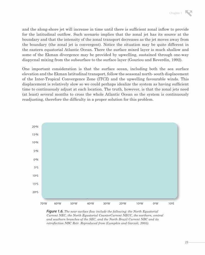
In this thesis we will focus on the role of wind forcing as a driver for the connection between the western boundary currents and the system of equatorial zonal currents (Figure 1.6). The study includes a careful analysis of different data sets in order to determine the dominant modes of oscillation for both wind forcing and ocean response. The principal hypothesis is that, over most of the western and central Atlantic, the wind-driven latitudinal divergence in the surface mixed layer is supplied through zonal convergence, originated from boundary currents such as the NBC. These boundary currents enter, or retroflect, into the interior ocean as zonal jets in geostrophic balance, therefore they are constrained by transatlantic lines of maximum (and minimum) sea surface height. The Ekman divergence, as calculated through the latitudinal Ekman transports across two adjacent lines of maximum sea surface height, may therefore be compared with the zonal transports that take place between them.

The physical mechanism in the western and central ocean may be idealized, for a one-and-a-half layer scenario, to occur as follows. The poleward Ekman transport simultaneously raises the upper-thermocline layers and depresses the free surface elevation (so that the cross-shore pressure gradients in the motion less lower layer remain negligible). As this happens the upper layer accelerates zonally in geostrophic balance. These cross-shore gradients

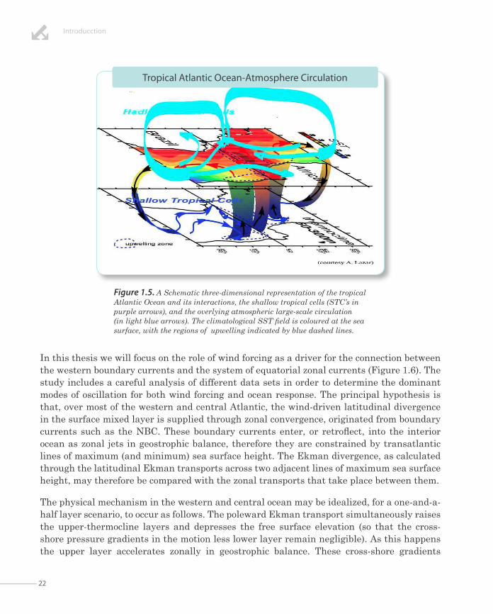
Figure 1.5. A Schematic three-dimensional representation of the tropical Atlantic Ocean and its interactions, the shallow tropical cells (STC’s in purple arrows), and the overlying atmospheric large-scale circulation (in light blue arrows). The climatological SST field is coloured at the sea surface, with the regions of upwelling indicated by blue dashed lines.

Tropical Atlantic Ocean-Atmosphere Circulation

23

Chapter 1

and the along-shore jet will increase in time until there is sufficient zonal inflow to provide for the latitudinal outflow. Such scenario implies that the zonal jet has its source at the boundary and that the intensity of the zonal transport decreases as the jet moves away from the boundary (the zonal jet is convergent). Notice the situation may be quite different in the eastern equatorial Atlantic Ocean. There the surface mixed layer is much shallow and some of the Ekman divergence may be provided by upwelling, sustained through one-way diapycnal mixing from the subsurface to the surface layer (Gouriou and Reverdin, 1992).

One important consideration is that the surface ocean, including both the sea surface elevation and the Ekman latitudinal transport, follow the seasonal north- south displacement of the Inter-Tropical Convergence Zone (ITCZ) and the upwelling favourable winds. This displacement is relatively slow so we could perhaps idealize the system as having sufficient time to continuously adjust at each location. The truth, however, is that the zonal jets need (at least) several months to cross the whole Atlantic Ocean so the system is continuously readjusting, therefore the difficulty in a proper solution for this problem.

Figure 1.6. The near-surface flow include the following: the North Equatorial Current NEC, the North Equatorial CounterCurrent NECC, the northern, central and southern branches of the SEC, and the North Brazil Current NBC and its retroflection NBC Retr. Reproduced from (Lumpkin and Garzoli, 2005).

20ºN

15ºN

10ºN

5ºN

0ºN

5ºS

10ºS

15ºS

20ºS

70ºW 60ºW 50ºW 40ºW 30ºW 20ºW 10ºW 0ºW 10ºE

24

Introducction

1.3. The Northwest Africa coastal upwelling region

In the eastern boundary of all major subtropical gyres we find the World’s largest upwelling systems (Figure 1.7). They are the sites where relatively cold and nutrient-rich subsurface waters reach the sea surface, with quite important consequences at regional, and even global scales: First, they lead to the onset of large primary production and, through the trophic chain, very important commercial fisheries [e.g., (Carr and Kearns, 2003)]; and, second, they transfer substantial amounts of heat from the atmosphere into the sea [e.g., (Pelegrí et al., 1997)]. In this thesis we will look at one of these upwelling systems, off Northwest Africa, that take place in the eastern margin of the North Atlantic subtropical gyre.

The Canary Current (CC) is traditionally thought to be the eastern boundary current of the North Atlantic subtropical gyre (Stramma, 1984; Stramma and Siedler, 1988) but the true eastern boundary condition for this gyre is the upwelling system off Northwest Africa. It has been shown that a large fraction of the interior ocean (about 3 Sv) recirculates south as the easternmost branch of the CC, the so called Canary Upwelling Current (CUC) (Pelegrí et al., 2005a; Machín et al., 2006; Laiz et al., 2012). The CUC feeds from the interior subtropical ocean and returns most of its flow to this subtropical gyre through intermittent filaments (such as in Cape Ghir and Cabe Bojador) and the permanent giant filament of Cape Blanc (Gabric et al., 1993; Pelegrí et al., 2005b); a relatively small fraction of this CUC may yet continue further south, across the Cape Verde frontal region, into the southern Cape Verde region (Peña- Izquierdo et al., 2012) (Figure 1.8).

The upwelling system consists of three main components [e.g., (Csanady, 1977, 982b; Pelegrí and Richman, 1993): (1) the upwelled waters, or nearshore band where subsurface waters have actually reached the sea surface, appears clearly in sea surface temperature (SST)

Figure 1.7. Eastern boundary currents and associated upwelling systems, respectively. From (http://www.meted.ucar.edu/)

25

Chapter 1

images as a coastal band of relatively cold waters; (2) the coastal upwelling front, as the surface signature of the baroclinic region, characterized by large normal-to-shore gradients in properties such as SST; and (3) the interior baroclinic ocean, where the geostrophic baroclinic jet is located because of the sea surface and upper thermocline maximum normal-to-shore gradients.

The above upwelling components were already present in the early two-dimensional steady-state solutions (Yoshida, 1955; Csanady, 1982; Gill, 1982) but the truth, as clearly illustrated by the SST images, is that upwelling is a highly complex threedimensional intermittent problem, with substantial along-shore variability. Intermittency and along-shore changes are indeed what characterize the complexity of coastal upwelling. They are the result of both the (spatial and temporal) variability of wind-forcing and the changes in coastal geomorphology.

The surface currents in upwelling regions also reflect this variability. The direct effect of the surface winds is to bring Ekman transport (and currents) in the surface mixed layer. However, in analogy to what happens for equatorial upwelling, this Ekman transport is divergent. The spatial non-homogeneity in Ekman transport (Ekman divergence) is high

44ºN

38ºN

32ºN

26ºN

20ºN

14ºN

8ºN

28ºW 22ºW 16ºW 10ºW 4ºW

Figure 1.8. The NW Africa region, showing the main currents (light blue: surface currents; dark blue: slope current), Cape Verde frontal zone (dashed blue lines) and mesoscale eddies (blue: cyclones; red: anticyclones) south of the Canary Islands. NACW: North Atlantic Central Water; SACW: South Atlantic Central Water; AC: Azores Current; CanC: Canary Current; MC: Mauritanian Current; NEC: North Equatorial Current; NECC: North Equatorial Countercurrent; PC: Portuguese Current; SC: Slope Current. Reproduced from Arístegui et al. (2009)

26

Introducction

in the coastal ocean as a result not only of wind non-homogeneities but, most important, because of the coastal constraint (Ekman transport goes to zero at the coast). There are two possible ways to provide for this divergence: the subsurface inflow at the coast (this being the most visible component of upwelling) and along-shore convergence.

The physical process may be visualized, for a one-and-a-half layer ocean, in a similar fashion as it occurs for the equatorial ocean. The cross-shore Ekman transport (together with the coastal constraint) raises the upper-thermocline layers and depresses the free surface elevation (the cross-shore pressure gfrom radients in the lower layer remain small), and the upper layer accelerates along-shore in geostrophic balance. These cross-shore gradients and the along-shore jet will increase in time until there is sufficient diapycnal mixing from the lower to the surface layer, which will also increase in time as a response to the shear between both layers, to provide for the cross-shore transport. If the problem is three-dimensional, as occurs in reality, some of the inflow may come from convergence in the along-shore jet; specifically, this happens when the along-shore jet exports water towards the interior ocean in the form of filaments.

The temporal scales for these transient processes are likely much shorter in the coastal upwelling region than in the equatorial Atlantic but we may expect that they will last long enough (one to two weeks) to idealize the solution as a succession of steady states. As for the equatorial ocean, the fundamental difficulty in finding a solution arises because of the transient character of the solution and the very impor tant spatial non-homogeneities.

1.4. Aims and outline of the dissertation

The principal aim of this doctoral dissertation is to improve our understanding on how the wind-driven surface Ekman divergence leads to spatial gradients in the surface elevation, capable of inducing surface currents in near-geostrophic balance. To this end, we study the spatial and temporal variability of the wind and its coupling with the upper ocean. The analysis is performed in two apparently very different dynamic regions; the coastal upwelling region off Northwest Africa and the equatorial upwelling system of the Tropical Atlantic Ocean. The analysis of each of these systems is carried out separately, structured in three chapters. Each chapter has its own set of conclusions, relative to the atmospheric forcing and ocean response within the regional context. Finally, in Chapter 5 the conclusions reached for both, coastal and equatorial, systems are critically compared and some general mechanisms are proposed.

27

Chapter 1

1.4.1. Coastal Ocean

Chapter 2

The Cape Blanc region is recognized as the most productivity in the NW Africa upwelling system. In order to obtain a good temporal and spatial resolution of the surface velocity field in the region, we implemented the Maximum Cross Correlation method for this region. This is done by adjusting the set of parameters used by the method, after applying a sensitivity analysis to provide the maximum area coverage and the best velocity resolution. As a result, the MCC technique allows us to obtain both daily and seasonal-mean (for both winter and spring) surface velocity images.

Chapter 3

We examine how changes in the wind patterns affect the surface currents and the intensity of upwelling in the Cape Blanc region. For this purpose we look at the weekly changes of two variables, the anomaly of the along-shore accumulative wind stress and a normalized coastal upwelling index, during winter and spring of two consecutive years. These are then related with the daily sea-surface temperature and surface velocity maps as obtained with the MCC method. The transient surface velocity fields are discussed in terms of the contribution of the surface Ekman velocity (the Ekman transport divided by the depth of the surface mixed layer) and the surface geostrophic velocity as inferred from satellite altimetry.

1.4.2. Open Ocean

Chapter 4

This chapter contains the second block of this work, focused on the tropical Atlantic: the system of near-surface zonal currents, their seasonal variability and their connection with the western boundary currents. Our objective is to better understand how the wind-driven Ekman transport is connected with the near-surface zonal currents. In the first part we carry out a complete spatial and temporal analysis of in situ, satellite, modelled and climatological data sets. In the second part, with the help of both a general circulation model and an idealized conceptual model, we analyze the surface ocean response to atmospheric forcing. In particular, we examine the importance of meridional Ekman divergence as a driver of the zonal currents and their temporal variability.

. .

. .

. .

. .

. .

. .

. .

. .

. .

. .

. .

. .

. .

. .

. .

. .

. .

. .

. .

. .

. .

. .

. .

. .

. .

. .

. .

. .

. .

. .

. .

. .

. .

. .

. .

. .

. .

. .

. .

. .

. .

. .

. .

. .

. .

. .

. .

. .

. .

. .

. .

. .

. .

. .

. .

. .

. .

. .

. .

. .

. .

. .

. .

. .

. .

. .

. .

. .

. .

. .

. .

. .

. .

. .

. .

. .

. .

. .

. .

. .

. .

. .

. .

. .

. .

. .

. .

. .

. .

. .

. .

. .

. .

. .

. .

. .

. .

. .

. .

. .

. .

. .

. .

. .

. .

. .

. .

. .

. .

. .

. .

. .

. .

. .

. .

. .

. .

. .

. .

. .

. .

. .

. .

. .

. .

. .

. .

. .

. .

. .

. .

. .

. .

. .

. .

. .

. .

. .

. .

. .

. .

. .

. .

. .

. .

. .

. .

. .

. .

. .

. .

. .

. .

. .

. .

. .

. .

. .

. .

. .

. .

. .

. .

. .

. .

. .

. .

. .

. .

. .

. .

. .

. .

. .

. .

. .

. .

. .

. .

. .

. .

. .

. .

. .

. .

. .

. .

. .

. .

. .

. .

. .

. .

. .

. .

. .

. .

. .

. .

. .

. .

. .

. .

. .

. .

. .

. .

. .

. .

. .

. .

. .

. .

. .

. .

. .

. .

. .

. .

. .

. .

. .

. .

. .

. .

. .

. .

. .

. .

. .

. .

. .

. .

. .

. .

. .

. .

. .

. .

. .

. .

. .

. .

. .

. .

. .

. .

. .

. .

. .

. .

. .

. .

. .

. .

. .

. .

. .

. .

. .

. .

. .

. .

. .

. .

. .

. .

. .

. .

. .

. .

. .

. .

. .

. .

. .

. .

. .

. .

. .

. .

. .

. .

. .

. .

. .

. .

. .

. .

. .

. .

. .

. .

. .

. .

. .

. .

. .

. .

. .

. .

. .

. .

. .

. .

. .

. .

. .

. .

. .

. .

. .

. .

. .

. .

. .

. .

. .

. .

. .

. .

. .

. .

. .

. .

. .

. .

. .

. .

. .

. .

. .

. .

. .

. .

. .

. .

. .

. .

. .

. .

. .

. .

. .

. .

. .

. .

. .

. .

. .

. .

. .

. .

. .

. .

. .

. .

. .

. .

. .

. .

. .

. .

. .

. .

. .

. .

. .

. .

. .

. .

. .

. .

. .

. .

. .

. .

. .

. .

. .

. .

. .

. .

. .

Chapter 2Winter and spring surface velocity

fields in the Cape Blanc region as deduced with the Maximum

Cross-Correlation technique*

*This chapter in impress as Castellanos, P., Pelegrí, J.L., Baldwin, D. Emery, W..J., Hernández-Guerra, A. (2013). Winter and spring surface velocity fields in the

Cape Blanc region as deduced with the Maximum Cross-Correlation technique. International Journal Remote Sensing, 34. DOI:10.1080/01431161.2012.716545

Winter and spring surface velocity fields in the Cape Blanc region as deduced with the Maximum Cross-Correlation technique

Abstract ................................................................................................. 31.

2.1.. Introducction ............................................................................ 32

2.2. MCC method - preview ....................................................... 34

2.3. The MCC method - set up for the Cape Blanc region ................................................... 37

2.3.1.. Data and implementation area ..................................37

2.3.2 . Advective versus diabatic changes ............................... 38

2.3.3. Sensitivity analysis ......................................................39

2.3.4. Removing spurious data .............................................42

2.4. Description of the surface flow in an upwelling area ......................................................44

2.4.1.. Instantaneous fields ...................................................45

2.4.2. Mean winter and spring fields ....................................47

2.5. Conclusions ......................................................................50

Acknowledgements ...............................................................51.

Chapter 2

31

31

Abstract

The ocean surface velocity field in the Cape Blanc region, off Northwest Africa, is investigated with the Maximum Cross-Correlation (MCC) method applied to channel-4 Advanced Very High Resolution Radiometer satellite images. An initial sensitivity analysis allows us to select the four parameters that provide maximum area coverage and best velocity resolution, while limiting the standard deviation for each velocity components within reasonable values. These are (m, n, MV, CT) = (22, 32, 50, 0.6), where m and n are the number of pixels of the search (SW) and reference (RW) windows, MV is the maximum possible velocity (in cm s-1), and CT is a correlation threshold for a feature to be tracked. Eight base images (one night and day image per season) are used to geometrically correct all images. A total of 489 images, for years 2005 and 2006, are analyzed and 106 velocity maps are generated with good coverage of the Coastal Transition Zone (CTZ), most of them for the winter (34) and spring (59) seasons. We remove spurious data using the method’s own filters (MV, CT, and a neighbour-vector comparison), requesting the velocity components to have Gaussian distributions and smoothing the resulting velocity fields with a median-vector filter. The instantaneous velocity maps illustrates the response of the alongshore coastal jet north of Cape Blanc (and its extension along the Cape Verde frontal region) to wind forcing, as well as numerous mesoscalar features (100 to 300 km wide) superposed on a westward offshore transport south of Cape Blanc. We also produce mean and standard deviation winter and spring velocity and Sea Surface Temperature (SST) fields. The along and offshore flow is better defined and more intense in spring than in winter, in concordance with cross-slope sharper temperature gradients during this season, and brings about a cooling of the whole region. Besides the existence of mesoscalar structures and offshore wind-induced flow, we identify five different ubiquitous currents: a south-westward jet north of Cape Blanc, a north-westward jet off Banc d’Argin, an offshore convergent jet, a spring jet-like feature at 18ºN, and a southward flow in the south-western CTZ.

32


32

2.1. Introduction

The remote inference of the ocean flow field started in the 1980’s, when several pioneering studies proved there is a close correspondence between sea-surface currents derived from infrared data collected with the Advanced Very High Resolution Radiometer (AVHRR) on the NOAA satellite series and the velocities estimated from drifters’ trajectories or measured with point current-meters (La Violette, 1984; Emery et al., 1986, 1992; Kelly, 1989). Two types of approach were used, in the first one the changes in the property field were analyzed under the light of some physical law, in the second one a property pattern was identified and its displacement was tracked. Both approaches examine the changes in the distribution of a property at the sea surface, as inferred from two time-consecutive images.

The first, or inverse, method aims at solving the advective equation governing the observed property (Kelly, 1989; Kelly and Strub, 1992; Vigan et al., 2000). However, the horizontal velocity field has two components so the solution may only provide one component of the flow field, unless two independent properties are used. Other innovative attempts that aim at identifying streamlines from individual images have had substantial success (Turiel et al., 2005), but are limited by the conditions that all surface features have to have a dynamic (rather than thermodynamic) origin and that the flow has to be stationary (so that stream-lines coincide with streak lines).

The second, or feature-tracking, method is based on identifying, segmenting and tracking structures in consecutive images. It assumes that any thermal structure in the ocean is produced through horizontal advection, structures may be rotated and deformed but cannot be created or destroyed. The most common featured-tracking technique application to the ocean has been the Maximum Cross-Correlation (MCC) method. The MCC technique was initially developed by Leese et al. (1971) to track cloud motions and was later adapted by Ninnins et al. (1986) to detect ice motion in the Beaufort Sea and by Emery et al. (1986) to estimate surface currents from the AVHRR images in the Vancouver area. The main limitation of this method is the availability of at least two good-quality satellite images, sufficiently close in time, with adequate sea coverage and spatial resolution.

AVHRR images are a good candidate as they are typically available once a day with 1 km resolution or twice daily with lower spatial resolution, although they are limited by meteorological factors such as atmospheric dust or clouds images. In this work, we will use the MCC feature tracking method, implemented for AVHRR images of the Cape Blanc region in the

Chapter 2

3333

eastern subtropical North Atlantic, to obtain instantaneous and mean surface velocity fields during winter and spring of 2005 and 2006 (Figure 2.1). In next Section, we briefly revise the fundamentals of the MCC, and in Section 2.3 we discuss the method’s set up for the Cape Blanc region, with details on specific requirements for setting the base images, the tracking parameters, and the vector filtering procedures. In Section 2.4, we present several instantaneous velocity maps as obtained with the method, together with their respective atmospheric forcing, and discuss the mean winter and spring sea surface temperature (SST and velocity fields. We end up with some major conclusions.

Figure 2.1. Image of NOAA16 satellite as obtained in the AVHRR reception station of the Physical and Remote Sensing Oceanography laboratory at ULPGC. The inset shows the Cape Blanc area where the MCC method has been implemented.

34


34

2.2. MCC method - preview

The MCC has been commonly applied to determine the surface ocean flow field through remote sensed thermal structures (e.g. Emery, et al., 1986, 1992, 2003; for a review see Marcello et al., 2008), although it is possible to use other properties such as ocean colour (García and Robinson, 1989; Crocker et al., 2007). Table 2.1 summarizes the previous MCC studies for determining surface flow patterns, indicating the property used for the analysis and the oceanic region considered. Major methodological advances were accomplished by Emery et al. (1992, 2003) through analyzing infrared brightness images, introducing an automatic image geo-referencing protocol and filtering out spurious velocity vectors. Several studies have carefully analysed the goodness and limitations of the method (Tokmakian et al., 1990; Emery et al., 1992; Marcello et al., 2008), generally obtaining high correlations between MCC-inferred velocities and those obtained with other indirect and direct methods, and concluding that the precision of the MCC method is between 0.1 and 0.2 m s-1 (Kelly and Strub, 1992; Gao and Lythe, 1998; Bowen et al., 2002).

Here we essentially follow the MCC method as explained in Emery et al. (1992, 2003). The infrared AVHRR images have about 1.1 km/pixel resolution and swap in five spectral channels. For the MCC application we use channel 4 (10.8-µm), which produces brightness-temperature images, because it allows more robust feature-tracking than imagery derived from the multichannel SST product (Bowen et al., 2002). The algorithm for processing the AVHRR images is divided into two main modules. The first one is the navigation, or geometric correction module, necessary for geo-referencing each individual image to an accurate map reference. This is done by geo-registering from a base image those same image elements that will appear in all other images. In this way the system automatically navigates each individual image through estimates of land displacement errors, i.e. it corrects each image for satellite-attitude roll, pitch and yaw parameters (Emery et al., 2003).

The second, or tracking, module computes the surfaces velocities. For this purpose it defines a structure and tracks its motion, and then applies several coherence filters. This tracking module employs four main parameters: a squared reference window (RW), a squared search window (SW), a maximum velocity (MV), and a correlation threshold (CT). The size of RW (m×m pixels) depends on the length of the individual mesoscalar structures in the study area, i.e. has to be large enough to enclose a full structure but not too large to include unwanted features. The size of SW (n×n pixels) is a function of the time lapse between images and the expected maximum surface currents in the region under consideration, i.e. it has to be at least as large as this velocity times the time interval between the images but it should be not too large to include undesired fortuitous high correlations (Emery et al. 1986, 2003, Kelly and Strub 1992, Wu and Emery et al. 2003).

Chapter 2

35

Table 2.1. Previous studies on sea surface circulation using the MCC. Acronyms for sensors are AVHRR (Advanced very High Reolution Radiometer), Coastal Zone Colour Scanner (CZCS), Ocean Colour Monitor (OCM), Sea-viewing Wide Field-of-view Sensor (SeaWiFS), and Moderate Resolution Imaging Spectroradiometer (MODIS).

AUTHORS AREA SENSOR

Emery et al. (1986) Northeastern Pacific AVHRR

García and Robinson (1989) English Channel AVHRR, CZCS

Kamachi (1989) Northwestern Pacific AVHRR

Tokmakian et al. (1990) Northeastern Pacific AVHRR, CZCS

Emery et al. (1992) Northwestern Atlantic AVHRR

Holland and Yan (1992) East and west US coast AVHRR

Kelly and Strub (1992) Northeastern Pacific AVHRR

Wu et al. (1992) East of New Zealand AVHRR

García Weil et al. (1994) Northeastern Atlantic AVHRR

Borzelli et al. (1999) Adriatic Sea AVHRR

Domingues et al. (2000) Southwestern Atlantic AVHRR

Afanasyev et al. (2002) Eastern Black Sea AVHRR

Barton (2002) West Australia AVHRR

Bowen et al. (2002) East Australian Current AVHRR

Kim and Sugimoto (2002) East China Sea AVHRR

Prasad et al. (2002) Indian Ocean OCM

Alberotanza and Zandonella (2004) Adriatic Sea AVHRR

Dransfeld et al. (2006) Global OceanGlobal area coverage

AVHRR

Crocker et al. (2007) Northeastern PacificAVHRR, SeaWifs

and MODIS

36


36

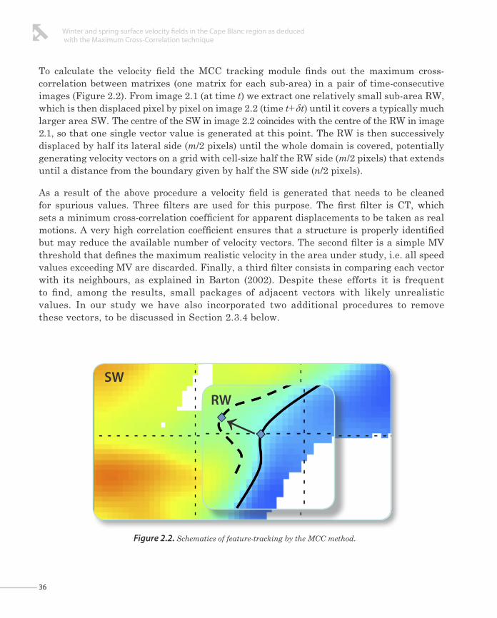
To calculate the velocity field the MCC tracking module finds out the maximum cross-correlation between matrixes (one matrix for each sub-area) in a pair of time-consecutive images (Figure 2.2). From image 2.1 (at time t) we extract one relatively small sub-area RW, which is then displaced pixel by pixel on image 2.2 (time t+δt) until it covers a typically much larger area SW. The centre of the SW in image 2.2 coincides with the centre of the RW in image 2.1, so that one single vector value is generated at this point. The RW is then successively displaced by half its lateral side (m/2 pixels) until the whole domain is covered, potentially generating velocity vectors on a grid with cell-size half the RW side (m/2 pixels) that extends until a distance from the boundary given by half the SW side (n/2 pixels).

As a result of the above procedure a velocity field is generated that needs to be cleaned for spurious values. Three filters are used for this purpose. The first filter is CT, which sets a minimum cross-correlation coefficient for apparent displacements to be taken as real motions. A very high correlation coefficient ensures that a structure is properly identified but may reduce the available number of velocity vectors. The second filter is a simple MV threshold that defines the maximum realistic velocity in the area under study, i.e. all speed values exceeding MV are discarded. Finally, a third filter consists in comparing each vector with its neighbours, as explained in Barton (2002). Despite these efforts it is frequent to find, among the results, small packages of adjacent vectors with likely unrealistic values. In our study we have also incorporated two additional procedures to remove these vectors, to be discussed in Section 2.3.4 below.

Figure 2.2. Schematics of feature-tracking by the MCC method.

SW

↓RW

Chapter 2

3737

2.3. The MCC method - set up for the Cape Blanc region

Any feature-tracking method has to be carefully implemented and calibrated before it may be successfully applied to a regional ocean. As explained above, for the MCC this implies, first, the definition of a base image to enable the automated processing of all other images and, second, a proper adjustment of several parameters until the calculated current field is self-consistent and coherent with the forcing meteorological fields. Once this is attained the method will not only describe the most common current patterns but will also help understand the ongoing dynamics. A proper implementation shall provide an optimal solution and will serve to understand the method's intrinsic limitations.

2.3.1.. Data and implementation area

The AVHRR images were gathered at the reception station in the Remote Sensing Center at the Universidad de Las Palmas de Gran Canaria. The multiple-infrared window channel data was corrected using regionally optimized algorithm coefficients (Eugenio et al., 2005), although channel 4 alone is used for calculating the brightness temperature. The SST images are used only to visually appreciate the dominant surface structures in our area of interest.

Table 2.2 illustrates the number of images eventually processed, after analyzing all available images for years 2005 and 2006. Infrared AVHRR images passes over the region are separated by 12-hour intervals, although some of these passes look at the region with angles quite far from Nadir and are discarded. Therefore, the number of processed images is 489 (329 in

YEAR 2005 2006

Processed images 329 160

generated maps 61 45

Winter maps 24 10

Spring maps 25 34

Summer maps 3 1

Fall maps 9 0

total images 489

total maps 106

Table 2.2. Number of processed images and generated velocity maps.

38


38

2005 and only 160 in 2006), about 34% of all possible images (1460 for two-year images every 12 hours). The images are grouped by season, each season spanning a three-month period as follows: December-February for winter, March-May for spring, June-August for summer, September-November for fall. This division lags the calendar year by about one month, chosen to take into account the thermal inertia in the northern hemisphere.

A base image is set to have 1024 × 1024 pixels, spanning the Cape Blanc region (from 15º N to 25º N and from 25º W to 15º W; Figure 2.1). In this manner a base image includes the African coastline along its eastern boundary and the Cape Verde Islands in the southwestern corner, so that several specific widely-distributed land-radiance features may be used for geo-referencing. Since the sea-land contrast in radiance usually changes dramatically with season and between day and night conditions (Emery et al., 2003), we use two base images per season, i.e. one per night and one per day conditions, for a total of eight base images (eight satellite-attitude files). This allows us to automatically process all day images; however, about 40% of the night images lack sufficient land-sea radiance contrast to exceed a threshold contrast required for detecting coastal geo-referencing features and, therefore, cannot be used to generate velocity maps.

2.3.2. Advective versus diabatic changesThe implicit MCC hypothesis is that the property of a water parcel (temperature if we use infrared images) is little modified during the time period between two consecutive images used to generate the velocity maps. During this time period the water parcel, if displaced adiabatically, should retain its upstream thermal characteristics, therefore bringing out an advective change. For the method to be successful this advective change, of the order of horizontal velocity times the heat-content horizontal gradient, has to be significantly larger than its diabatic change. Therefore, before proceeding to implement the method, it is convenient to get first-order estimates of the advective and diabatic transformations in our region of interest.

One important characteristic of the Cape Blanc region is that during winter the surface waters undergo relatively low heat gain from the atmosphere, in contrast with maximum values in late summer. Typical values are 20 W m-2 for winter, 80 W m-2 for spring and fall, and 160 W m-2 in summer (Bunker, 1976; Hsiung, 1986; Schmitt et al., 1989; Pelegrí et al., 1997). This energy flux is to be distributed over the surface mixed-layer, which is typically about 50 m in the deep ocean and several times thicker offshore from the upwelling front. Therefore, the maximum energy flux per unit volume becomes δe/δt, i.e. the change in internal energy per unit volume δe gained during a time interval δt. In winter δe/δt = (20 W m-2)/(50 m) = 0.4 Joules m-3 s-1, increasing by a factor of eight in summer. This flux is related to the rate of change of potential temperature δθ through δe/δt = ρ cp δθ/δt, where ρ is water

Chapter 2

3939

density and cp is specific heat. At sea-surface pressure and for typical seawater salinities cp @ 4000 J kg-1 ºK-1, so that the temperature change is given by about δθ = 10-7 δt ºC s-1, with δt in seconds. For a time lapse δt = 1 day ≈ 105 s, this relation gives δθ ≈ 0.01 ºC in winter, 0.04 ºC in spring and fall, and 0.08 ºC in summer.

These values are to be compared with typical changes associated to the advection of structures in a region with some background spatial temperature gradient. In the Cape Blanc Coastal Transition Zone (CTZ), a band several-hundred kilometers wide which comprises those waters from the coastline to the deep ocean, the temperature ranges from 18 to about 23 ºC and the mean zonal gradient is about 5 ºC / 500 km, so an advective change related to a velocity of order 0.1 m s-1 would be 10-6 ºC s-1 or about 0.1 ºC day-1. Far offshore, however, the temperature gradients are much smaller, typically 1ºC / 500 km, so the advective change there would only be about 0.02 ºC day-1. Therefore the error involved with thermodynamic changes is relatively small in the CTZ during all seasons except summer, but further offshore it may be as large as the advected signal at all seasons.

2.3.3. Sensitivity analysisTo carry out the sensitivity analysis we select two images separated by 12 hours, corresponding to 23 and 24 March 2005 (Figure 2.3). In these two figures we may appreciate relatively cold waters that run all along the African continent, characteristic of wind-induced coastal upwelling, and the offshore export of these cold waters near Cape Blanc by a surface filament (Pelegrí et al., 2006; Pastor et al., 2008).

The sensitivity analysis aims at finding the best combination of parameters that control the output velocity maps for the Cape Blanc region. The specified parameters are those four previously discussed: RW, SW, CT and MV. We use a very simple approach, which consists in setting three reasonable values for each parameter and examining the output from all possible combinations. Table 2.3 shows the number of pixels for RW and SW, and the MV and CT values used for these sensitivity tests.

For each output map we consider the number of vectors generated, N, and their mean correlation coefficient ȓ, and calculate the mean zonal and meridional velocities (u, v) and their standard deviations (σu , σv ). We also calculate the equivalent number of pixels Np for the generated vectors: since the size of each cell in the grid of generated vectors is m/2 then Np = N (m/2)2 . The latter number, Np , is a measure of the actual area where we are generating velocity information while the former, N, provides information of the spatial resolution of these vectors, i.e. given equal Np the greater N the better will be the spatial resolution of the velocity distribution. The ideal scenario is to have a case with relatively low dispersion (both σu and σv must remain less than the mean expected velocities for the area) and high values of both Np and N.

40


40

Table 2.4 shows the results for all possible combinations, after requiring the condition n>m to be satisfied. The cases are identified as (m, n, MV, CT), where m and n are the number of pixels of RW and SW, respectively, and MV is given in cm s-1. There is no trivial way to select one realization over another, except for case (22, 32, 90, 0.6) as it has standard deviations substantially greater than for all other cases (more than twice the mean surface currents which are about 0.1 m s-1 for the area, e.g. Pastor et al., 2008) and may be discarded. In order to help select the best output we draw a scatter plot of the standard deviations

Parameters

MCC

Size RW

(m x m)

Size SW

(n x n)

Treshold MV

(cm s-1)

Cut-off

Correlation

Index CT

Values

18x18 22x22 50 0.4

22x22 32x32 60 0.6

32x32 45x45 90 0.8

Table 2.3. Number of pixels for the reference (RW) and search (SW) windows, maximum velocity (MV), and correlation threshold (CT) used for the sensitivity tests.

Figure 2.3. Sequence of two SST images (23 and 24 March 2005) used for the regional implementation sensitivity tests. . The color-coded scale displays de SST in ºC. The area shown is the one marked in Figure 2.1.

Chapter 2

4141

(σu , σv ) as a function of both N and Np (Figure 2.4). The bottom panel of Figure 4 shows there are three cases that have very similar Np values (close to 60000, Table 4) while the top panel of this figure shows that for only two of these cases N remains high (close to 500, Table 2.4).

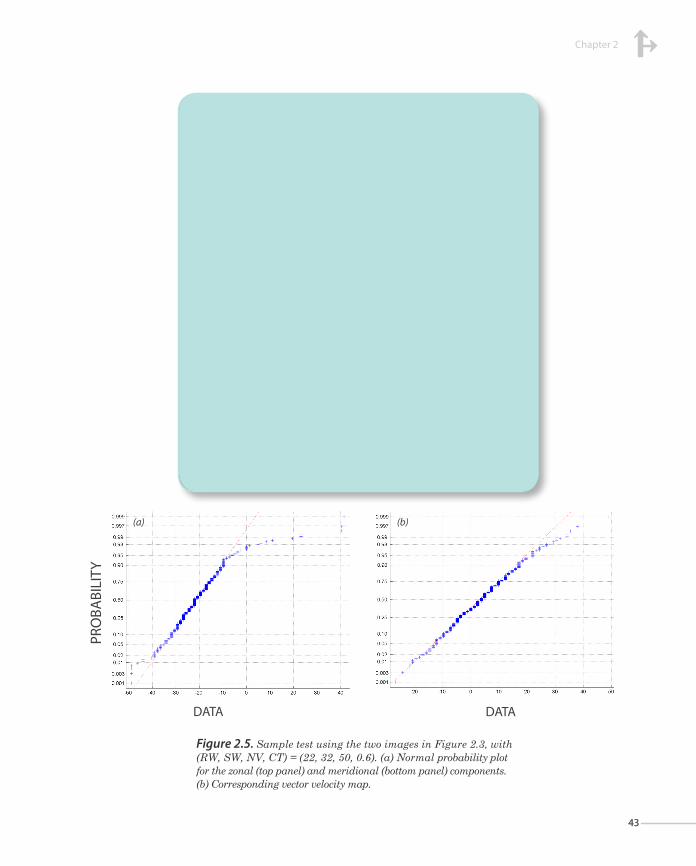
From the above procedure it turns out that the two best cases are (22, 32, 50, 0.6) and (22, 32, 60, 0.6). To further discern between these two cases we construct the probability density function (pdf) of each velocity component and look at how well it fits a Gaussian distribution through a normal probability plot. The best fit corresponds to (22, 32, 50, 0.6) (Figure 2.5), which is chosen to be the optimum combination of MCC parameters for the Cape Blanc region. This set of parameters is used to routinely generate all velocity maps to be discussed in the remainder of this paper.

NVelocities

(u, v) ( σu , σv )ȓ Np

Parameters

values

699 -18.772 3.154 15.283 14.847 0.834 12582 (18, 22, 50, 0.6)

377 -19.902 2.671 10.186 12.306 0.903 6786 (18, 22, 50, 0.8)

556 -19.323 2.351 14.663 14.472 0.841 10008 (18, 32, 60, 0.6)

249 -18.137 1.771 14.056 12.684 0.910 4482 (18, 45, 90, 0.8)

479 -20.691 3.799 10.615 10.655 0.842 57959 (22, 32, 50, 0.6)

489 -20.283 3.926 12.941 11.733 0.841 59169 (22, 32, 60, 0.6)

546 -17.234 1.251 26.664 21.445 0.836 66066 (22, 32, 90, 0.6)

281 -19.895 2.522 11.522 11.22 0.901 34001 (22, 32, 60, 0.8)

379 -20.055 3.837 9.659 12.311 0.849 45859 (22, 45, 60, 0.6)

235 -20.575 3.260 10.634 10.621 0.857 28435 (22, 45, 90, 0.8)

229 -20.201 4.306 11.984 14.534 0.907 58264 (32, 45, 90, 0.6)

Table 2.4. Number of vectors generated, N, the equivalent number of pixels Np , and their mean correlation coefficient ȓ ; corresponding mean zonal and meridional velocities (u, v) and their standard deviations (σu , σv ).

Note: The cases are identified as m × n × MV × CT, where m and n are the number of pixels of SW and RW, respectively, and MV is given in cm s-1. Only those combinations with n > m are shown.

42


42

2.3.4. Removing spurious dataTable 2.2 shows the number of maps eventually generated, with (m, n, MV, CT) = (22, 32, 50, 0.6), from all available satellite images. The number of summer and fall images is very limited as these seasons are characterized by very high cloud coverage. Such extensive cloud conditions occur following sea-induced cooling of the air masses and subsequent water vapour condensation, further intensified in the CTZ.

As explained in Section 2.2, the MCC method incorporates three filters which are applied to each individual velocity map in order to remove spurious velocity vectors: the CT value, the MV threshold, and a next-neighbour comparison filter. In this study we have implemented two additional filters. The first-one consisted in an iterative procedure that adjusts a Gaussian distribution to each velocity component and removes all values beyond three standard deviations (hereafter named 3-σ filter). The procedure is as follows: (1) compute the probability density function (pdf), (2) find out the closest Gaussian distribution, (3) remove all data values beyond three standard deviations of the adjusted Gaussian distribution, (4) iterate until no further data removal was necessary. When the computed pdf distribution gets close enough to a Gaussian distribution the iteration ends up, typically one iteration is sufficient.

Figure 2.4. Scatter plot of the standard deviations (σu , σv ) (crosses and cicles) respectively as a function of (a) the number of generated vectors, N, and (b) the equivalent number of pixels, Np . Note: The three best cases are encircled, the optimal one in read: (m, n ,MV ,CT ) = (22, 32, 50, 0.6).

Stan

dard

dev

iatio

n cu

rren

t ve

loci

ty [c

m/s

]

N

(*ustd) (o vstd) funcion of N vector (*ustd) (o vstd) funcion of Np vector

Np (x10^4)

(a) (b)

Chapter 2

4343

Figure 2.5. Sample test using the two images in Figure 2.3, with (RW, SW, NV, CT) = (22, 32, 50, 0.6). (a) Normal probability plot for the zonal (top panel) and meridional (bottom panel) components. (b) Corresponding vector velocity map.

Probability

Probability

Data

Data

PRO

BABI

LITY

DATA

Probability

Probability

Data

Data DATA

(a) (b)

44


44

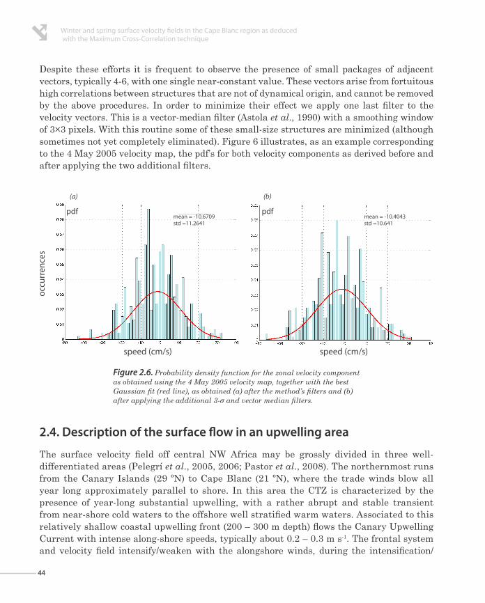
Despite these efforts it is frequent to observe the presence of small packages of adjacent vectors, typically 4-6, with one single near-constant value. These vectors arise from fortuitous high correlations between structures that are not of dynamical origin, and cannot be removed by the above procedures. In order to minimize their effect we apply one last filter to the velocity vectors. This is a vector-median filter (Astola et al., 1990) with a smoothing window of 3×3 pixels. With this routine some of these small-size structures are minimized (although sometimes not yet completely eliminated). Figure 6 illustrates, as an example corresponding to the 4 May 2005 velocity map, the pdf’s for both velocity components as derived before and after applying the two additional filters.

Figure 2.6. Probability density function for the zonal velocity component as obtained using the 4 May 2005 velocity map, together with the best Gaussian fit (red line), as obtained (a) after the method’s filters and (b) after applying the additional 3-σ and vector median filters.

2.4. Description of the surface flow in an upwelling area

The surface velocity field off central NW Africa may be grossly divided in three well-differentiated areas (Pelegrí et al., 2005, 2006; Pastor et al., 2008). The northernmost runs from the Canary Islands (29 ºN) to Cape Blanc (21 ºN), where the trade winds blow all year long approximately parallel to shore. In this area the CTZ is characterized by the presence of year-long substantial upwelling, with a rather abrupt and stable transient from near-shore cold waters to the offshore well stratified warm waters. Associated to this relatively shallow coastal upwelling front (200 – 300 m depth) flows the Canary Upwelling Current with intense along-shore speeds, typically about 0.2 – 0.3 m s-1. The frontal system and velocity field intensify/weaken with the alongshore winds, during the intensification/

speed (cm/s)

pdf

occu

rren

ces

speed (cm/s)

pdfmean = -10.6709std =11.2641

mean = -10.4043std =10.641

(a) (b)

Chapter 2

4545

weakening periods there are offshore/onshore surface transports which bring normal-to-shore displacements of the upwelling front (Pelegrí and Richman, 1993).

The central area is the Cape Verde frontal zone, which runs from Cape Blanc to the Cape Verde Islands, where the upper-thermocline North Atlantic and South Atlantic waters meet (top 600 to 700 m). This frontal system, in contrast with the coastal upwelling front, does not display intrinsic substantial temperature gradients. The temperature contrasts frequently arises, however, because of the offshore extension of the coastal branch of the Canary Current, the Canary Upwelling Current, along the Cape Verde front. This extension brings offshore relatively cold coastal waters from Cape Blanc, what is known to be the Cape Blanc filament (Gabric et al., 1993). The frontal system is quite unstable, with frequent meandering and lateral intrusions that show-off as substantial mesoscale variability superposed onto the dominant south-western along-front flow.

The most meridional area is located south of the Cape Verde frontal system. Here we find a relatively weak northward coastal branch associated to the Guinea Dome cyclonic gyre (Pradhan et al., 2006). South of Cape Blanc wind-driven upwelling only predominates during winter and, to a lesser degree, in spring. Upwelling is more intermittent and the most common situation is that of fluctuating offshore Ekman flow combined with mesoscalar instabilities generated near-shore or at the Cape Verde frontal zone (Pastor et al., 2008).

2.4.1.. Instantaneous fields

Let us briefly examine three instantaneous surface velocity fields that illustrate the above patterns (Figure 2.7). The insets in this figure illustrate the wind surface stress as obtained from daily values of the microwave radar in the QuikSCAT satellite (0.5º resolution). In all three cases most available vectors correspond to a several-hundred thick band adjacent to the coastline (the CTZ) and, to a lesser degree, to the Cape Verde frontal zone.

The left panel in Figure 2.7 shows the velocity field for 21 March 2005. This is a typical winter situation, with sustained intense surface wind stress reaching south of Cape Blanc, as far as Cape Verde. The wind is particularly intense along the Cape Verde frontal zone, which causes offshore transport along this frontal system, as suggested by SST maps (Figure 3 shows these maps for two days later). The region south of this frontal system is dominated by Ekman offshore velocities, with little mesoscalar structure.

The central panel in Figure 2.7 corresponds to the 24 April 2005 situation, characteristic of a transition between winter and spring conditions. The surface wind field is yet dominated by the north-easterly trade winds over the whole region, but has strengthened in Cape Blanc and the northern area and weakened further south. The dominant velocity pattern comes

46


46

from the alongshore coastal upwelling jet which appears to even penetrate south of Cape Blanc. This corresponds to sustained wind-induced coastal upwelling, with Ekman transport building up large cross-shore pressure gradients which then drive an intense along-shore geostrophic flow (e.g. Pelegrí and Richman, 1983). The southern CTZ displays relatively small (100 km diameter) and weak (less than 0.1 m s-1) mesoscale features, with no apparent predominant mean flow.

Figure 2.7. Surface velocity maps obtained for (a) 21 March 2005, (b) 24 April 2005, and (c) 4 May 2005. The insets show the daily QuikSCAT wind surface stress for those same dates, the color code in the right inset (N m-2) applies to all panels.

↓1 m/s

↓1 m/s

↓1 m/s

(a) (b)

(c)

Chapter 2

4747

The right panel in Figure 2.7 corresponds to 4 May 2005, a common spring situation. The forcing is similar to the previous one but the wind has substantially weakened south of Cape Blanc. The northern coastal jet departs from the coast near Cape Blanc, with little southward penetration. In the CTZ south of Cape Blanc the mesoscalar structures are considerably large (200-300 km diameter) and intense (about 0.2 m s-1), suggesting a complex interacting pattern with intensifying and weakening convergent and divergent motions.

2.4.2. Mean winter and spring fieldsDuring winter (December to February) and spring (March to May) we have a sufficient number of maps (34 for winter, 59 for spring, Table 2.2) to produce mean surface velocity fields. Figure 8 illustrates the mean speed and its standard deviation for each season. These variables are calculated at each grid point (with lateral side of 22 pixels, the size of the reference window) as an average of all data values within the grid cell. The mean speed is estimated as ( ͞u 2+ ͞v 2 )1/2 and the standard deviation i s obtained as

The mean zonal and meridional velocity components are given by ͞u =Σ ui and ͞v =Σ vi , where i indicates a velocity value from one velocity map, j is the number of available vectors for the season and the summation is over all vectors available for the season. For these calculations we have used only those points with a minimum of five velocity vectors.

Figure 2.8 illustrates how the mean surface speed gets intensified during spring as compared with winter. In wintertime the speed is typically less than 5 cm s-1 in the CTZ and only exceeds 10 cm s-1 in some offshore points. In spring the flow intensifies both in the CTZ and offshore, particularly off Cape Blanc and along the south-westward offshore extension of the Cape Blanc filament. During both seasons the standard deviation is quite large, indicative of large temporal variability as a result of substantial mesoscalar activity in the region. During winter the standard deviation exceeds the mean values almost everywhere while in spring both mean and standard deviation are of similar magnitude. Maximum values of both mean and standard deviation typically occur in the offshore extension of the Cape Blanc filament while the minimum values are found in the CTZ between Cape Blanc and Cape Verde.

Figure 2.9 presents a vector map with the mean surface velocity field per season, calculated using the same above procedure, where we have emphasized the most coherent flows. The predominant features are a south-westward jet along the slope north of Cape Blanc that extends until the edge of the mean image, and a north-westward jet starting at about 18 ºS and extending along the slope of Banc d’Argin. This pattern is most evident during spring but yet present in winter, the two jets converging offshore (beyond 19 ºW) as an offshore jet centered at about 20 ºN in winter and 20.5 ºN in spring. South of 18 ºN the flow is predominantly

{(1/j)Σ [(ui- ͞u )2 + (vi- ͞v )

2]}1/2j

i=1j

i=1

j

i=1

48


48

offshore, with a winter jet-like feature centered at about 18 ºN. During both seasons the south-western CTZ also exhibits a weak southward flow.

In Figure 2.9 we also show the mean SST fields for the Cape Blanc area as obtained using all available 2005 and 2006 images per season (Table 2.2). A remarkable feature for the Cape Blanc region is the apparent sea surface cooling of spring as compared with winter. These local situation must be viewed in a wider geographical context, over all NW Africa, where spring SST is generally warmer than winter SST (Figure 2.10). A plausible explanation is precisely the presence of these swift along-slope and offshore jets during the spring season. These coastal jets collect and eject offshore, to a great deal through the Cape Blanc giant filament, the relatively colds upwelled waters, being capable of cooling down the whole CTZ.

Figure 2.8. (Left) Magnitude and (right) standard deviation of the surface velocity field for (top) winter and (bottom) spring of the 2005 – 2006 period, as obtained with the MCC.

SPRING

WIN

TER

mean s.d.

25

20

15

10

05

Chapter 2

4949

Figure 2.9. Mean surface velocity field for (left) winter and (right) spring of the 2005 – 2006 period, as obtained with the MCC. The insets show the corresponding mean SST field. The features discussed in the text are indicated: southwestward jet north of Cape Blanc (I), northwestward jet off Banc d’Argin (II), offshore convergent jet (III), spring jet-like feature at 18 ºN (IV), and southward flow in the souhwestern CTZ (V).

SPRING

WINTER

50


2.5. Conclusions

The Maximum Cross-Correlation method has been successfully implemented to process channel-4 images from the Advanced Very High Resolution Radiometer (AVHRR) sensor in NOAA satellites, for the Cape Blanc region off NW Africa. The method uses four parameters which need to be carefully tuned before it may be routinely implemented, these are (m, n, MV, CT), where m and n are the number of pixels of the search (SW) and reference (RW) windows, MV is the maximum velocity trusted to be real (given in cm s-1), and CT is a correlation threshold that the RW has to find in the SW for a moving feature to be identified. For this purpose we use the 23 and 24 March 2005 images, select different reasonable values for each parameter and examine the results for all possible combinations. The best set of parameters is established from the standard deviations of the zonal and meridional velocity components, (σu , σv ), the number of generated vectors N and the equivalent number of pixels Np. The best fit is to have reasonably small standard deviations, good sea coverage (large Np ) and good resolution (N ), which turns out to be (22, 32, 50, 0.6).

Figure 2.10. Mean SST for January 2005 and April 2005 off NW Africa, as characteristic images for the winter and spring periods.

25 23 21 19 17 15

Jan 2005 Apr 2005

25 23 21 19 17 15

Jan 2005 Apr 2005 Jan 2005

25 23 21 19 17 15

Jan 2005 Apr 2005 Apr 2005

Chapter 2

51

Once the control parameters are established, the MCC method may be routinely applied to all images available images (with a minimum of sea-surface coverage). The method is first georeferenced using eight base images, one night and one day image per season, and then applied to all 2005 and 2006 images. A total of 489 images have been processed and 106 velocity maps generated. These maps are further processed to remove spurious values through two additional filters: a 3-σ filter, which consists in fitting a Gaussian distribution to the probability density functions of each velocity component and iterating until all velocities beyond three standard deviations are removed, and a vector-median filter with a smoothing window of 3×3 pixels.

The resulting maps are useful to describe the surface dynamics of the Coastal Transition Zone (CTZ) but are unable to give useful information from the deep ocean. We present several examples of velocity maps that provide a good visualization of the instantaneous fields in the CTZ. These maps show a predominance of the alongshore coastal jet north of Cape Blanc and its extension along the Cape Verde frontal region, and the existence of numerous mesoscalar features (100 to 300 km wide) superposed on a westward offshore transport south of Cape Blanc, the relative intensity of these features responding to the surface wind stress.

We have finally combined all seasonal maps to produce winter and spring mean velocity fields. The results show a more intense and better defined flow in spring than winter, in concordance with the mean Sea Surface Temperature (SST) images for these seasons that display more intense temperature gradients over the CTZ. These jets collect and distribute offshore, mainly through the Cape Blanc giant filament, relatively cold upwelled water, being the plausible cause of a spring local decrease in SST. Up to five different jets superpose onto the mean offshore wind-induced flow: a south-westward jet north of Cape Blanc, a north-westward jet off Banc d’Argin, an offshore convergent jet, a spring jet-like feature at 18 ºN, and a southward flow in the south-western CTZ. The flow field is, however, quite variable possibly as a result of the wind-intermittency and the mesoscalar activity. This is reflected by the standard deviation maps which often have values that exceed the mean speeds.

Acknowledgements

The authors are grateful to Biswajeet Pradhan and an anonymous reviewer for useful comments. Funding for this work comes from the Ministerio de Ciencia e Innovación, Spain, through project “Memoria Oceánica del Clima: mecanismos y rutas de formación de aguas superficiales en el Atlántico ecuatorial” (MOC2, ref. nº. CTM2008-06438-C02-01).

. .

. .

. .

. .

. .

. .

. .

. .

. .

. .

. .

. .

. .

. .

. .

. .

. .

. .

. .

. .

. .

. .

. .

. .

. .

. .

. .

. .

. .

. .

. .

. .

. .

. .

. .

. .

. .

. .

. .

. .

. .

. .

. .

. .

. .

. .

. .

. .

. .

. .

. .

. .

. .

. .

. .

. .

. .

. .

. .

. .

. .

. .

. .

. .

. .

. .

. .

. .

. .

. .

. .

. .

. .

. .

. .

. .

. .

. .

. .

. .

. .

. .

. .

. .

. .

. .

. .

. .

. .

. .

. .

. .

. .

. .

. .

. .

. .

. .

. .

. .

. .

. .

. .

. .

. .

. .

. .

. .

. .

. .

. .

. .

. .

. .

. .

. .

. .

. .

. .

. .

. .

. .

. .

. .

. .

. .

. .

. .

. .

. .

. .

. .

. .

. .

. .

. .

. .

. .

. .

. .

. .

. .

. .

. .

. .

. .

. .

. .

. .

. .

. .

. .

. .

. .

. .

. .

. .

. .

. .

. .

. .

. .

. .

. .

. .

. .

. .

. .

. .

. .

. .

. .

. .

. .

. .

. .

. .

. .

. .

. .

. .

. .

. .

. .

. .

. .

. .

. .

. .

. .

. .

. .

. .

. .

. .

. .

. .

. .

. .

. .

. .

. .

. .

. .

. .

. .

. .

. .

. .

. .

. .

. .

. .

. .

. .

. .

. .

. .

. .

. .

. .

. .

. .

. .

. .

. .

. .

. .

. .

. .

. .

. .

. .

. .

. .

. .

. .

. .

. .

. .

. .

. .

. .

. .

. .

. .

. .

. .

. .

. .

. .

. .

. .

. .

. .

. .

. .

. .

. .

. .

. .

. .

. .

. .

. .

. .

. .

. .

. .

. .

. .

. .

. .

. .

. .

. .

. .

. .

. .

. .

. .

. .

. .

. .

. .

. .

. .

. .

. .

. .

. .

. .

. .

. .

. .

. .

. .

. .

. .

. .

. .

. .

. .

. .

. .

. .

. .

. .

. .

. .

. .

. .

Chapter 3Wind-driven surface circulation

in the Cape Blanc region*

* This chapter has been submitted to Continental Shelf Research as Castellanos, P., Pelegrí, J.L., Benazzouz, A. Wind-driven surface circulation

in the Cape Blanc region.

. .

. .

. .

. .

. .

. .

. .

. .

. .

. .

. .

. .

. .

. .

. .

. .

. .

. .

. .

. .

. .

. .

. .

. .

. .

. .

. .

. .

. .

. .

. .

. .

. .

. .

. .

. .

. .

. .

. .

. .

. .

. .

. .

. .

. .

. .

. .

. .

. .

. .

. .

. .

. .

. .

. .

. .

. .

. .

. .

. .

. .

. .

. .

. .

. .

. .

. .

. .

. .

. .

. .

. .

. .

. .

. .

. .

. .

. .

. .

. .

. .

. .

. .

. .

. .

. .

. .

. .

. .

. .

. .

. .

. .

. .

. .

. .

Wind-driven surface circulation in the Cape Blanc region

Abstract ................................................................................................. 55

3.1. Introducction ............................................................................ 56

3.2. Data set ......................................................................................... 59

3.3. Methods ........................................................................................ 60

3.3.1. Ekman transport and wind impulse ...........................61

3.3.2. Geostrophic currents ......................................................... 62

3.3.3. Coastal upwelling index ................................................... 62

3.3.4. MCC technique ............................................................63

3.4. Time series of wind forcing and upwelling index ......................................................63

3.4.1. Wind forcing ................................................................63

3.4.2. Coastal upwelling indexes ..........................................65

3.5. Ocean surface patterns during specific events ...................................................69

3.5.1. Sea surface temperature ............................................69

3.5.2. Surface currents ..........................................................72

3.6. Mean winter and spring ocean surface fields .......................................................79

3.7. Concluding remarks ......................................................81

Acknowledgements ...............................................................83

Chapter 3

55

55

Abstract

We analyze the short-term transition, on time scales of the order of days and weeks, of the surface fields in the coastal transition zone off Northwest Africa, between 15ºN and 25ºN, during winter and spring 2005 and 2006. This is a complex region characterized by the baroclinic coastal jet north of Cape Blanc, along-shore convergence and water export at the Cape Blanc giant filament, and substantial mesoscale variability between Capes Verde and Blanc. Here we use the anomalies of the wind impulse and a normalized coastal upwelling index, evaluated off 17ºN, 20ºN and 23ºN, in order to assess the importance of wind forcing in this short-term variability. We also employ daily and weekly surface maps of wind, temperature, surface height and currents to investigate which are the mechanisms that lead to the relatively fast changes in the flow patterns. The coastal baroclinic jet and the Cape Blanc giant filament are ubiquitous features, the two being intrensically related through the intensity of upwelling off Cape Blanc. Therefore, the strenght of both features to a large extent responds to the fluctuations of the northeasterly winds; their intensity is greater in spring than winter but during both seasons they experience relatively fast oscillations related to the intermittency of the wind field. The mesoscalar features are visible in all the domain, with time scales typically of the order of two weeks, but become prominent in the southern part of the domain during spring, apparently related to the appearance of a quite intense northward coastal jet south of Cape Blanc.

56


56

3.1. Introduction

The surface and upper thermocline waters off Northwest (NW) Africa conform the eastern boundary of the North Atlantic subtropical gyre, one of the World’s large scale eastern boundary current systems. This boundary region is characterized by the presence of intense coastal upwelling which leads to very high levels of primary production and supports important fisheries [e.g., Carr and Kearns, 2003]. The relevance of upwelling goes well beyond the continental shelf and slope, as it interacts with the deep-ocean boundary system and brings about very complex dynamic features, covering what has been termed the Coastal Transition Zone (CTZ). The NW Africa offshore region has received significant attention in the past, with many studies aimed at understanding the large-scale characteristics of upwelling [e.g., Mittelstaedt, 1983, 1991; Van Camp et al., 1991; Müller and Siedler, 1992; Gabric et al., 1993; Klein and Tomczak, 1994; Barton et al., 1998; Hagen, 2001; Lazaro et al., 2005] and its interaction with the interior ocean [e.g., Elmoussaoui et al., 2005; Hagen, 2005; Pelegrí et al., 2005a,b, 2006; Machín et al., 2006; Pastor et al., 2008, 2012; Mason et al., 2011; Peña-Izquierdo et al., 2012; Laiz et al., 2012], and some other studies more focused on providing detailed descriptions of specific local processes [e.g., Barton et al., 1989; Gabric et al., 1993; Arístegui et al., 1994; Barton et al., 2004; Benítez-Barrios et al., 2011; Mason et al., 2012].

The intensity of upwelling along NW Africa responds to the seasonal north-south migration of the surface winds associated to the North Atlantic atmospheric pressure systems, specifically the Azores High. Upwelling takes place as the coastal winds have an equatorward component which drives Ekman seaward transport in the surface mixed layer, so that these surface waters are replaced by relatively cold and nutrient-rich subsurface waters. The northeasterly, or trade, winds are permanent all year-long between Cape Blanc and the Canary Islands, but reach north to the Iberian Peninsula in summer and south to Cape Verde in winter (hereafter all seasons refer to the northern hemisphere). The seasonal evolution of the wind regime along the African coast and its relation with the intensity of coastal upwelling, as inferred by the temperatures at the sea surface in the coastal region, have been studied by several authors [Wooster et al., 1976; Speth and Detlefsen, 1982; Mittlestaedt, 1991; Nykjaer and Van Camp, 1994; Hernandez-Guerra and Nykjaer, 1997; Pardo et al., 2011; Benazzouz et al., 2012; Marcello et al., 2012]. These works find good agreement between monthly-mean wind indexes, such as the cross-shore Ekman transport, and monthly-mean upwelling indexes, defined in terms of the temperature difference between nearshore and offshore waters; the

Chapter 3

5757

upwelling index, however, typically lags the Ekman index by about one month, reflecting the temporal memory of the whole boundary system [Nykjaer and Van Camp, 1994].

Most studies of the coastal upwelling system off NW Africa have indeed focused on this large-scale seasonal response, as if the coastal ocean would respond to (quite idealized and unrealistic) slowly changing winds. However, the actual instantaneous statemay be very different from what could be expected from such a slow transition, as upwelling exhibits relatively fast transients in response to the wind intermittency [e.g., Csanady, 1982a; Gill, 1982]. This is vividly shown by the sea surface temperature (SST) satellite images, with changes in the SST and surface currents taking place in time scales as short as a few days [e.g., Csanady, 1977, 1982b; Pelegrí and Richman, 1993, 1994]. For example, as an upwelling-favourable wind develops not only the offshore Ekman transport will intensify but also the cross-shore slope of the sea surface will increase and, with it, the along-shore baroclinic coastal current. Additionally, the winds and coastline are usually far from homogeneous in the along-shore direction which drives the three-dimensionality in the SST and surface current fields.

In this work we will focus on the short-scale temporal response of a very complex upwelling region off NW Africa, from Cape Verde to south of the Canary Islands, or about 14ºN to 26ºN (Fig. 3.1). The region under study is quite complex as it includes three subregions with very distinct dynamics: (a) the waters of the North Atlantic subtropical gyre recirculate in the eastern boundary as the Canary Current (CC) and its easternmost branch, the Canary Upwelling Current (CUC), before reaching back into the interior ocean as the North Equatorial Current (NEC) [e.g., Pelegrí et al., 2005; Pastor et al., 2012]; (b) waters originated in the southern subtropical gyre, although substantially transformed as they pass through the equatorial an tropical Atlantic Ocean, which reach the south of Cape Blanc through the eastward extension of the North Equatorial Counter Current (NECCC) and recirculate cyclonically in the Cape Verde Basin around the Guinea Dome [e.g., Lazaro et al., 2005; Peña-Izquierdo et al., 2012]; and (c) the convergence near Cape Blanc of waters of northern and southern origin, along what has been named the Cape Verde frontal zone [Zenk et al., 1991], and the subsuequent offshore water export of upwelled waters over a distance of several hundred of kilometers as the Cape Blanc giant filament [Gabric et al., 1991].

Our objective is to identify the short-term response of the surface ocean to wind forcing in each of these three regions. For this purpose we will use remote-sensed surface data for the whole region and along three specific normal-to-shore transects, as well as daily surface current fields as obtained through a local implementation of the Maximum Cross Correlation (MCC) technique. In particular, we will investigate the weekly changes in sea-surface wind stress and coastal upwelling index during the winter and spring seasons and will also examine the spatial distribution of SST and surface currents during several specific events. Our study will be limited to the winter and spring seasons as this is the time when upwelling reaches

58


58

south of Cape Blanc and the MCC method allows to extract daily surface current fields with good spatial and temporal coverage. These near-instantaneous fields will be interpreted in terms of their Ekman (or wind-induced) and geostrophic contributions, and will eventually be compared to the seasonal mean (winter and spring) surface fields.

The paper is organized as follows. Section 3.2 and 3.3 present the data sets and the methodologies developed for the study. Section 4 shows the time series of several indexes for wind forcing and SST response at three different locations which charac terize the three main upwelling subregions. Sections 3.5 and 3.6 respectively examine the surface circulation daily and seasonal patterns, decomposed in terms of their Ekman and geostrophic contributions, emphasizing the similarities and differences between the instantaneous and seasonal fields. The paper ends up with some over all assessments on the predominant dynamic mechanisms in section 3.7.

Figure 3.1. Schematics of the surface and upper-thermocline currents (solid lines with arrows) in the region off Cape Blanc in November 2008, adapted from Peña-Izquierdo et al. [2012]. The thick dashed lines represents the location of the CapeVerde frontal zone. The three latitudes used to characterize the wind forcing and upwelling response, and the main geographic features, are identified.

Chapter 3

5959

3.2. Data set

In this work we have used two different types of data for the time period from January to June of 2005 and 2006, encompassing the region from 14ºN to 26ºN and from 15ºW (or the African coastline) to 22º W (Fig. 3.1): (1) satellite data for SST, absolute dynamic topography (ADT), surface geostrophic velocity and wind stress, and (2) climatological data for the mixed layer depth (MLD).

The sea surface height (SSH) is obtained from altimeter data after correcting for the ocean tides and the surface atmospheric pressure. The Absolute Dynamic Topography (ADT) is calculated as the deviation of SSH from the Earth’s geoid, or that portion of the elevation of the sea surface that responds to the ocean currents. The ADT and geostrophic surface velocity fields are directly obtained from the Archiving, Validation and Interpretation of Satellite Oceanographic (AVISO) web site (http://www.aviso.oceanobs.com) through the SSALTO/DUACS system which combines altimetric data from several satellites. Data are available with a 0.5° resolution in latitude and longitude with a temporal resolution of one week.

Wind data are measured by the SeaWinds Scatterometer on board the QuikSCAT satellite. The daily and mean wind fields, averaged for selected periods, are available from the Center for Satellite Exploitation and Research (CERSAT) at the Institut Français de Recherche pour l’Exploitation de la Mer (IFREMER) (cersat.ifremer.fr). In this study we use the Level-4 daily products of sea-surface wind stress fields (absolute value and horizontal components), available on a 0.5° resolution in latitude and longitude.

The SST measurements come from the Advanced Very High Resolution Radiometer (AVHRR) of the National Oceanic and Atmospheric Administration (NOAA). This data set is produced jointly, from the original AVHRR data, by the Rosenstiel School of Marine and Atmospheric Science at the University of Miami and NOAA and distributed in several formats (www.nodc.noaa.gov/sog/pathfinder4km/); here we have usedthe 4-km resolution weekly data set (version 5). Additionally, the original AVHRR images (typically two images per day) were received at the reception station of the Remote Sensing Center at the Universidad de Las Palmas de Gran Canaria (ULPGC), where they were corrected using regionally optimized algorithm coefficients in order to calculate the brightness temperature [Castellanos et al., 2012].

Finally, the MLD monthly climatological fields are available from the National Oceanographic Data Center (NODC) [de Boyer Motégut et al., 2004] on a 2º grid in latitude and longitude. There are several possible criteria to define the MLD. Here we have chosen the so-called temperature criterion, which defines the MLD as the depth where the temperature changes 0.2°C with respect to the temperature at a reference depth of 10 m.

60


60

3.3. Methods

In order to characterize the intensity of coastal upwelling, we have selected three zonal transects (17ºN, 20ºN and 23ºN) where the wind stress and the normal-to-shore SST distribution are examined. The center transect has been chosen slightly south of Cape Blanc (20º50’N) as the 20ºN parallel crosses the continental shelf on the location where it extends further offshore. The other two transects, equidistant from the central one, have been selected to be completely within the two dynamic regimes found north and south of the Cape Verde front.

Through the analysis of satellite images covering the shelf and offshore regions, from 15ºN to 25ºN and from 15ºW to 22ºW, we may obtain the surface velocity fields with the MCC technique. Under the assumption that the non-linear terms in the momentum equations are relatively small, the (subinertial) surface velocity field may be expressed as the combination of the wind-induced and geostrophic velocity fields. The wind-induced contribution is deduced from the surface wind stress while the surface geostrophic velocity is deduced from the sea surface elevation. All these surface velocity fields may be calculated for weekly, monthly and seasonal intervals.

In this work we will look at the time series of wind forcing and surface response, as well as to the spatial response patterns of specific events, during 2005 and 2006 (Table 3.1). Our analysis on short-term variability will be centered on winter (January through March) and spring (April through June) because upwelling becomes intensified south of Cape Blanc during these two seasons.

Table 3.1. The left column shows the events discussed in the text; the dates used for each analysis are indicated. The right column shows the total number of available winter and spring images per year, used to generate the mean winter and spring surface current fields.

EVENTSMEAN FIELDS

MCC and wind-induced currents

Weekly geostrophic currents Eight-days SST and NCUI values

21-24 March 2005 16-22 and 23-29 March 2005 14-21 March 2005 Winter 2005

24 Winter 2006

10

28 March 2006 23-29 March 2006 22-29 March 2006

24-25 April 2005 21-27 April 2005 23-30 April 2005

Spring 2005 25

Spring 2006 34

24-26 April 2006 20-26 April 2006 23-30 April 2006

3 May 2005 28 April to 4 May 2005 1-8 May 2005

4 May 2006 28 April to 4 May 2006 1-8 May 2006

Chapter 3

6161

3.3.1. Ekman transport and wind impulse

If the wind stress at the sea surface is substantially larger than the internal interfacial stresses, the zonal UE and meridional VE Ekman transports may be estimated from the momentum equations as

where (τy , τx ) is the wind stress (two-dimensional) vector at the sea surface, with τx the zonal component (West-East, positive eastwards) and y the meridional component (South-North, positive northwards), ρ is the water density and f is the Coriolis parameter. A reasonable assumption is that this Ekman transport takes place exclusively in the surface mixed layer, i.e., wind exerts its influence not only to mix properties as temperature and salt but also to mix momentum and, as a result, the whole surface mixed layer will move with the same velocity. With this suposition we may estimate the Ekman velocity simply as the Ekman transport divided the depth of the mixedlayer,

(uE , vE ) = 1/h (UE , VE)

For the mixed layer depth we have used the NODC monthly climatological MLD.

Additionally, in order to analyze those conditions favourable for coastal upwelling, the sea-surface wind stress is decomposed into alongshore and cross-shore winds at three selected latitudes: 17ºN, 20ºN, and 23ºN. The wind stresses used for this analysis are taken at the grid coordinate closest to the coast; since the wind data has a 0.5º resolution this means that the wind-stress values represent the conditions in a cell centered near 25 km from the coastline. The continental shelf in our area of study has a mean width of about 30 km, therefore a cell centered some 25 km from the coastline represents that the wind is located close to the shelf break, which is most adequate for our analysis. The coast is closely aligned in the South-North direction up to the latitude of Cape Blanc and beyond this latitude it takes an orientation tilted about 23º from the true north. Therefore we have chosen the meridional wind stress component as the along-shore meridional wind stress at 17ºN and 20ºN, and the projection of the wind-stress vector onto a coordinate system rotated clockwise by 23º as the along-shore meridional wind stress at 23ºN.

In our study region, with northeasterly winds, the mean state of upwelling is the result of a balance between the wind stress at the sea surface and the retarding forces, such as (a) friction with the underlying waters and the sea floor and (b) a northward pressure gradient because of water pile-up towards the south. We are most interested in those instances when the system is found out of balance, typically because of an increase or decrease in the upwelling winds, with the retarding frictional forces rapidly changing in order to find a new force balance. A simple way to assess the deviations from the mean upwelling state, whether

(UE , VE ) = (τy – τx )

ρf

62


62

it is reinforced or weakened, is by calculating the along-shore wind impulse [Csanady, 1978], defined as

where τy here refers to the along-shore wind stress. This variable represents the accumulative effect of the along-shore wind stress, for constant along-shore wind it will lead to a straight line of constant slope which is to represent the mean conditions. A comparison with expression (1) shows that the wind impulse actually is the time in tegral of the cross-shore Ekman transport, therefore temporal increases or decreases in the slope of the along-shore wind impulse will respectively represent periods of enhanced or weakened upwelling.

3.3.2. Geostrophic currents

The difference between SSH with respect to the Earth’s geoid correspond to that portion of the elevation of the sea surface that responds to the ocean currents, this is the ADT. The field of geostrophic surface velocities (u , v) in the zonal x and meridional y directions may be

derived from the ADT field ƞ (x , y) as

where g is the gravity acceleration.

3.3.3. Coastal upwelling index

The normalized coastal upwelling index (NCUI) is used as an indicator for the local strength of upwelling, in this work it is calculated weekly using 4-km resolution AVHRR images. The index, a function of latitude θ and time t, is based on the normal-to-shore SST distribution (between the coastline and 2000 km offshore) [Demarcq and Faure, 2000; Benazzouz et al., 2006]:

where Tmin is the minimum SST temperature measured within a coastal band 50 km wide, Tmax

is the maximum monthly temperature within a 2000 km band from the coast (obtained from the climatology), and Tup is the absolute minimum monthly temperature at each grid point, as determined from the weekly SST minimum values for the 1991- 2009 period [Benazzouz et al., 2006].

NCUI (θ , t)=Tmax (θ , t) - Tmin (θ , t)Tmax (θ , t) - Tup (θ , t)

(u , v ) = - , fg ∂ƞ

∂x∂ƞ∂y( ) ( )

I = ʃτy dt

Chapter 3

6363

3.3.4. MCC technique

The MCC method is an automated technique that calculates the surface circulation fields by tracking the horizontal displacement experienced by surface features between time-consecutive images [Emery et al., 1992, 2003]; the AVHRR images are available separated by 24- hour intervals and with a horizontal 1.1 km resolution. The procedure was applied to brightness temperature, channel 4 (10.8 μm), as it is most robust to track surface features [Bowen et al., 2002]. The implementation of the MCC to the Cape Blanc region is explained in Castellanos et al. [2012]. In summary, the method uses four parameters: a squared (m x m pixels) reference window that de fines the size of features, a squared (n x n pixels) search window for feature-match, a maximum possible value v for the surface velocity, and a correlation threshold c for matching features beyond which the search is considered successful. The selected combination of parameters is (m, n, v, c) = (22, 32, 0.5 m s-1, 0.6) [Castellanos et al. 2012].

3.4. Time series of wind forcing and upwelling index

3.4.1. Wind forcingThe temporal variability of the near-shore horizontal wind-stress vector at the three latitudes for the period January-June of 2005 and 2006 is shown in Figure 3.2. For both years we may appreciate in all transects a predominance of the northerly winds. The most variable conditions occur between January and March, characterized by periods of intensified wind lasting between 1 and 3 weeks followed by a sudden wind weakening, and even occasional wind reversals, that typically last one week. During these months the wind stress values display substantial spatial coherence with maximum values at 17ºN. During the April-June period the northerly winds remain more constant in time, with slightly less intensity at 17ºN during the last two months; nevertheless, there are still short periods, a few days long, when the wind weakens. These fluctuations in wind intensity, with relatively long periods of persistent winds followed by shorter periods of wind relaxation, have been reported by several authors [e.g., Gabric et al., 1993; Nykjaer and Van Camp, 1994]. The data also suggests the existence of some interannual variability in the wind stress, with more intense winds in 2006 than in 2005.

The along-shore wind-stress follows a pattern similar as described above, with persistent mean northerly winds but with substantial weekly variability. A close up for the period between March and May is shown in Figure 3.3. We may appreciate the latitudinal shift of the maximum winds with time: the wind stresses are largest at 17ºN in March, have similar values at all latitudes in April and become most intense at 23ºN in May.

64


64

Figure 3. 2. Daily surface wind stress vectors off the coastline at 17º N, 20º N and 23º N as determined from QuikSCAT during the January-June period of 2005 (top panel) and 2006 (bottom panel).The events discussed in the text are identified as gray vertical bars.

Chapter 3

6565

The time integration of the along-shore wind stress, defined as the along-shore wind impulse (equation 2), is an excellent way to summarize this variability. In Figure 3.4 we separately plot the along-shore wind impulse I for all three latitudes and for both 2005 and 2006. In all cases I has a general decreasing trend as a result of the ubiquitous northerly winds (its absolute value increases with time) with subtle but significant differences with location and time. The best way to appreciate these differences is by adjusting, through a least square fit, a linear function to each curve so that the most relevant information is contained in the slope of the curve and in the temporal changes of the residuals obtained by substracting the original variable to the adjusted linear function (hereafter named wind-impulse anomalies).

3.4.2. Coastal upwelling indexes

The temporal changes in the wind-impulse anomalies are, to a great extent, reflected in the time series of the NCUI (Figs. 3.4 and 3.5). There is a generalized increase during the first three months of the year followed by a decrease during the following three months, with intermittent variations typically 10-15 days long. In particular, the NCUI displays a prominent maximum towards the end of March in 2005 at 20ºN and 23ºN which parallels the behavior of the wind-impulse anomaly. Further, both the wind-impulse anomaly and the

Figure 3.3. Along-shore wind stress component off the coastline at 17ºN, 20ºN and 23ºN asdetermined from QuikSCAT during the period from March to May of 2005 (top panel) and March to May of 2006 (bottom panel). Negative values represent equatorward winds.The events discussed in the text are identified as gray vertical bars.

Win

d St

ress

(N m

-2)

66


66

Figure 3.4. The six panels present the distribution of the wind impulse and its anomaly for three selected nearshore locations at 23ºN (top panels), 20ºN (middle panels) and 17ºN (lower panels) during 2005 (left panels) and 2006 (right panels). Each panel is divided into two subpanels. The first subpanel shows the time integration of the alongshore wind stress (wind impulse) from January to June (black line): The dotted curve corresponds to the wind impulse daily values while the solid line shows the linear fit to the data, on each subpanel the equation of the linear fit is presented. The second subpanel shows the wind-impulse anomalies, or residuals, calculated as the actual wind impulse less the linear fit.

Chapter 3

6767

NCUI have values substantially larger in 2005 than in 2006 (in contrast with the slope of the linear fit which is larger in 2006 than in 2005).

The main difference between both variables is that the NCUI has a better defined seasonal at 23ºN in 2006, with a prominent peak by the end of March in the NCUI which is not reflected at all in the anomaly. Nevertheless the similarity is striking and points at the potential use of the wind-impulse anomaly as a proxy for the upwelling index.

The time series for both variables, NCUI and wind-impulse anomaly, indicate that the temporal change in the intensity of upwelling is about the same north and south of Cape Blanc; this contrasts with the slope of the linear fit to the wind impulse which is actually significantly greater south than north of Cape Blanc. This presents a novel perspective when compared with previous studies which emphasized that the seasonal alternation in the intensity of upwelling is most pronounced south of Cape Blanc [Mittelstaedt, 1991; Van Camp et al., 1991; Nieto et al., 2012].

Figure 3.5. Normalized coastal upwelling index at 23ºN, 20ºN and 17ºN (top, middle and bottom panels) from January to June during 2005 (left panels) and 2006 (right panels).

68


March April May

26

24

22

20

18

16

May26

24

22

20

18

16

-22 -20 -18 -16

April

-22 -20 -18 -16

March26

24

22

20

18

16

-22 -20 -18 -16

Figure 3.6. Monthly-mean geostrophic (top panels) and wind-induced (bottom panels) surface currents during March, April and May 2005. The geostrophic vectors are superposed onto the colour-coded ADT.

Chapter 3

69

3.5. Ocean surface patterns during specific events

Under the assumption that the non-linear (or advective) momentum terms are relatively small, it turns out that the variability of the subinertial surface flow (at frequencies shorter than the daily and inertial periods) is entirely determined by the variability of the wind-induced and geostrophic contributions. In order to appreciate the typical wind-induced and geostrophic spatial structures we present the monthly-mean fields for March, April and May 2005 (Fig. 3.6). It is clear that the two mean contributions have very different spatial patterns: the wind-induced currents are quite homogeneous over the whole region but the geostrophic currents are characterized by mesoscale features, of the order of a few hundred kilometers. Regarding the temporal scales, the mesoscale features typically change at time scales of a few weeks so that only a few structures last from one month to another, such as the cyclonic eddy northwest of Cape Verde between March and April (Fig. 3.6).

In this section we will examine the response of the SST and surface flow fields to different wind forcings as illustrated by six individual events. The dates of each event differ slightly depending on the analysis carried out, so hereafter they will be identified with the dates of the MCC images (Table 3.1). The events are chosen because of the availability of surface currents as obtained from the MCC and because of their distinctive characteristics. The wind fields (and therefore the wind-induced currents) are daily but the (eight-day) SST images and the (weekly) altimetry fields are for those periods closest in time to the MCC current fields. We will see how the mesoscale structures may induce current reversals at any specific point within time scales typically about two weeks. In contrast, the spatial changes in the wind-induced currents are relatively smooth although they may also display significant temporal intermittency, at time scales of a few weeks, with intensification or weakening of the offshore flow. The two contributions are profoundly related through the coastal baroclinic jet, which is induced by the along-shore winds but very soon becomes in geostrophic balance [Pelegrí and Richman, 1993]. We will see that the combination of both contributions, geostrophic and wind-induced, provides the character of the surface currents in the region: a mean offshore large-scale field with the superposed intense mesoscale variability.

3.5.1. Sea surface temperatureA good perspective of the CTZ and the intensity of upwelling is provided by the weekly-averaged SST images and the corresponding NCUI values (latitude-dependent); in Figure 3.7 we present these for each of the six events analyzed. The SST maps provide a view of the offshore extension of the upwelling region and, to a smaller degree, the presence of mesoscalar features within the CTZ. The NCUI, which is corrected by the latitudinal and monthly changes in the intensity of upwelling (equation 4), also tells us whether the observed coastal upwelling is stronger or weaker than the expected upwelling at each latitude and season.

70


70

a

c

e

b

d

f

Figure 3.7. Weekly coastal upwelling indexes (right panels) and sea surface temperature fields (left panels) for the following weeks: (a) 14-21 March 2005, (b) 23-30 March 2005, (c) 1-8 May 2005, (d) 22-29 March 2005, (e) 23-30 March 2006, and (g) 1-8 May 2006.

Chapter 3

7171

The 21-24 March 2005 event corresponds to the end of a period of sustained upwelling winds over the whole region, attaining maximum values south of Cape Blanc and weakening north of Cape Blanc (Figs. 3.2 and 3.3). The time series of wind impulse and NCUI at the three reference latitudes (17ºN, 20ºN and 23ºN) confirm that it corresponds to a period of intense upwelling (Figs. 3.4 and 3.5). The SST maps and latitudinal distribution of the NCUI for the week of 14 to 21 March 2005 illustrate the existence of generalized upwelling north of 15ºN, with large values of the NCUI and the presence of many filament-like structures emanating from the upwelled region into the CTZ (Fig. 3.7a).

The 24-25 April 2005 event corresponds to a few days of weak winds, following a period when the winds progresively weakened over the whole region (Figs. 3.2 and 3.3). The wind-impulse anomalies are relatively small, as compared with the 21-24 April 2005 event, yet remain positive at 23ºN and 20ºN but turn into negative at 17ºN (Fig. 3.4). This temporal evolution is reflected in the NCUI values which experience a substantial decrease at all latitudes (Fig.3.5). The 23 to 30 April 2005 SST maps evidence the existence of intense/weak upwelling north/south of 17ºN, in agreement with the latitudinal distribution of the NCUI (Fig. 3.7b). The existence of intense upwelling in the northern region brings about a very well defined frontal zone; this baroclinic front would be associated to an intense southward coastal baroclinic jet, likely responsible for substantial along-shore convergence and the observed prominent offshore extension of the Cape Blanc giant filament off about 20ºN.

The 3 May 2005 event corresponds to the end of a period with moderate intensification of the upwelling winds (Figs. 3.2 and 3.3). This is clear in the slight recovery of the (positive) anomalies of wind impulse at all latitudes (Fig. 3.4) and in the maintenance of relatively high NCUI values during this same period, followed by a substantial decrease of both variables after mid May 2005 (Fig. 3.5). The 1 to 8 May 2005 SST map and the NCUI latitudinal distribution are very similar to those for the previous event between 15ºN and 25ºN except for the weakeaned filament at 20ºN (Fig. 3.7c).

The 28 March 2006 event has some resemblances to the 21-24 March 2005 event but in this case the upwelling winds have intensified north of Cape Blanc and weakened in the southern region (Figs. 3.2 and 3.3). The wind-impulse anomalies and the NCUI values have relatively large values, yet they are substantially smaller than during the 2005 analogous event (Figs. 3.4 and 3.5). The 22 to 29 March 2006 SST maps and NCUI latitudinal distribution is, to a great extent, quite similar to the one observed in the March 2005 event, again displaying the existence of numerous filament-like structures (Fig. 3.7d). However, upwelling has strengthened in the northern portion of our study area (near 25ºN) and has weakened towards the southern end (near 15ºN).

The 24 to 26 April 2006 event again resembles the 24-25 April 2005, with the winds weakening at all latitudes (Figs. 3.2 and 3.3). The wind forcing shows some differences: during the 2005 event the wind-impulse anomalies were positive at 20ºN and 23ºN but during the April 2006

72


72

events they are negative at all latitudes, indicating a weakening of the along-shore winds at levels below the mean winter-spring values (Fig. 3.4). This substantial decrease during the April 2006 event is also reflected by a quite sharp reduction in the NCUI values at all latitudes (Fig. 3.5). The 23 to 30 April 2006 SST image shows that the upwelling band extends all the way to 15ºN, although not very intense, somewhat reflected by the moderately high values of the NCUI all along the coast (Fig. 3.7e).

Finally, the 4 May 2006 event takes place during a time of relatively weak mean winds but immediately after an intensification that lasted just a few days (Figs. 3.2 and 3.3). This is reflected in a short recovery of both the wind-impulse (Fig. 3.4) and the NCUI (Fig. 3.5) at the reference latitudes. This recovery is seen in the SST maps and in the NCUI latitudinal distribution for the 1 to 8 May 2006 period: the upwelling north of Cape Blanc is not as intense as in 2005 but becomes most prominent between Capes Verde and Blanc (Fig. 3.7f).

The results confirm that the coastal SST field has little inertia, its intensity substantially changing after just a few days with different wind conditions. At times of intense winds (such as in March) the initially sharp surface front is followed by the offshore extension of cold waters into the interior ocean through surface filaments. The predominant seasonal spatial patterns share some similarities from one year to another, yet with substantial interannual variability; in our case upwelling was generally more intense in 2005 than in 2006, although in several instances upwelling was best developed in the region south of Cape Blanc during 2006. One specific feature in the NCUI latitudinal distribution is a systematic decrease at about 20ºN; this is likely related to the presence of the shallow and relatively warm waters over the Banc d’Argin, which suggests that at this latitude the minimum SST temperature should be better calculated within a coastal band wider than 50 km.

3.5.2. Surface currentsAll winter and spring images of 2005 and 2006 have been examined and those that satisfy some minimum requirements of cloud-free area have been selected for the application of the MCC method [Castellanos et al., 2012]. Eventually a total of 34 winter and 59 spring images have been generated (Table 1). In this subsection we present and discuss the most relevant characteristics of the surface current fields corresponding to six different events. The total fields are inferred with the MCC technique (section 3.3.4) while the wind-induced and geostrophic contributions are calculated as discussed in sections 3.3.1 and 3.3.2. Recall the MCC method is applied to subsequent (24 hours apart) brightness temperature images so we get daily surface current values. The wind-induced contribution is also obtained daily, from the QuikSCAT wind fields, and is presented as a top inset on each map. The geostrophic contribution is derived from the closest weekly-altimetry map, specifically from the ADT products from AVISO, and is presented as a bottom inset on at least one map of each sequence.

Chapter 3

7373

The wind-induced currents for the 21 to 24 March 2005 event are always in the off shore direction, with maximum values exceeding 0.6 m s-1 off Cape Blanc, and tend to intensify between Capes Verde and Blanc (the Cape Verde basin) towards the end of the period. For this event we present the geostrophic surface currents for the 16-22 and 23-29 March 2005 periods. One major feature is the southward coastal jet that initially (during the week of 16-22 March) runs south between about 23ºN and 18ºN, i.e., over the region where the offshore winds have intensified, and later (by the week of 23-20 March) becomes diverted offshore at about 22ºN; during this second week the flow between 19ºN and 21ºN has actually reverted and flows north. Other smaller mesoscalar features are also present offshore in the northern part of the domain, likely related to the Canary eddy corridor [Sangrà et al., 2009], and in the southeastern end of the domain. The total currents, as inferred through the MCC method, follow the geostrophic pattern but spatially smoothed as a result of the more homogeneous wind-induced contribution: the coastal jet north of Cape Blanc, its offshore extension at the latitude of Cape Blanc, the progressive appearance of the northward coastal jet between 19ºN and 21ºN, and the relatively small mesoscalar features in the Cape Verde basin; these mesoscalar structures are very noticeable on 21 March but appear to decrease in the following days, as the wind currents in this southern region become intensified (Fig. 3.8).

The 24 and 25 April 2005 event present a situation where moderately intense wind induced seaward currents, with maximum values about 0.5 m s-1, take place off and north of Cape Blanc. The geostrophic surface currents, corresponding to the 21-27 April 2005 period, endorse the existence of the coastal jet north of Cape Blanc and its offshore extension just south of Cape Blanc, as well as the existence of relatively large and weak cyclonic patterns in the Cape Verde basin. These two predominant patterns are confirmed by the MCC-inferred currents (Fig. 3.9).

The 3 May 2005 event corresponds to a situation with moderate wind-induced seaward currents over the whole region, with maximum values about 0.5 m s-1. The geostrophic currents, for the 28 April to 4 May 2005 period, display relatively weak currents in the whole CTZ except for a small intense cyclonic eddy just south of CapeBlanc, approximately over the Bank d’Argin. The MCC field reflects the lack of intense mesoscalar structures, with not prominent or coherent features except for a moderate southward coastal jet in the region north of Cape Blanc (Fig. 3.10).

The 28 March 2006 event illustrates the existence of relatively intense wind-induced currents, up to about about 0.5 m s-1, north of Cape Blanc but extensively weakening towards the south. The geostrophic field does not display significant features in the CTZ except for the presence of a nearshore dipole which leads to a seaward intense jet at about 20ºN. The MCC technique could not calculate sufficient surface velocity vector north of Cape Blanc but south of this latitude the calculated currents are mostly directed seaward, reflecting the predominance of the wind-induced contribution and the lack of any intense mesoscalar

74


74

Figure 3.8. Daily surface currents as determined using the MCC method between 21 and24 March 2005. The top insets show the wind-induced surface velocity vectors and the bottom insets show the weekly geostrophic vectors on top the colour-coded ADT field.

15º N

22º W

25º N

15º W

15º N

22º W

25º N

15º W

15º N

22º W

25º N

15º W

15º N

22º W

25º N

15º W

Chapter 3

7575

15º N

22º W

25º N

15º W

15º N

22º W

25º N

15º W

Figure 3.9. Daily surface currents as determined using the MCC method for 24 and 25 April 2005. The top insets show the wind-induced surface velocity vectors and the bottom insets show the weekly geostrophic vectors on top the colour-coded ADT field.

structures (Fig. 3.11). The 24 to 26 April 480 2006 event presents a situation where very intense seaward wind induced currents, with maximum values close to 0.8 m s-1, take place off and north of Cape Blanc. The geostrophic surface currents, corresponding to the 20-26 April 2006 period, display a clear southward coastal jet between about 25ºN and 19ºN, again related to the location of the maximum offshore wind-induced currents. Near 20ºN, at about the location of the Cape Blanc giant filament, we find a prominent seaward jet. The MCC-inferred surface currents indeed confirm the existence of both the northern coastal jet and a wide region of latitudinal convergence towards the 20ºN latitude (Fig. 3.12).

76


76

15º N

22º W

25º N

15º W

15º N

22º W

25º N

15º W

Figure 3.11. Surface currents as determined using the MCC method

for 28 March 2006. The top insets show the

wind-induced surface velocity vectors and

the bottom inset shows the weekly geostrophic

vectors on top the colour-coded ADT field.

Figure 3.10. Surface currents as determined using the MCC method for 3 May 2005. The top inset show the wind-induced surface velocity vectors and the bottom inset shows the weekly geostrophic vectors on top the colour-coded ADT field.

Chapter 3

7777

Figure 3.12. (previous and current page)Daily surface currents as determined using the MCC method between 24 and 26 April 2006. The top insets show the wind-induced surface velocity vectors and the bottom insets show the weekly geostrophic vectors on top the colour-coded ADT field.

15º N

22º W

25º N

15º W

15º N

22º W

25º N

15º W

15º N

22º W

25º N

15º W

78


78

Figure 3.13. Surface currents as determined using the MCC method for 4 May 2006. The top insets show the wind-induced surface velocity vectors and the bottom inset shows the weekly geostrophic vectors on top the colour-coded ADT field.

Finally, the 4 May 2006 event corresponds to a situation with wind-induced currents similar to the 3 May 2005 event but, according to the 28 April to 4 May 2006 altimetry image, with a much intens coastal jet north of Cape Blanc, a very prominent seaward filament off Cape Blanc, and substantially mesoscale geostrophic currents elsewhere. Notice this event takes place in the middle of a short period (a few days long) of intensification of the wind regime, which must have reinforced the coastal jet and the along-shore water convergence near Cape Blanc, leading to offshore water ejection through the Cape Blanc giant filament. This event also illustrates how different the mesoscalar field can be from one instance to another, without any evident reason for such differences (Fig. 3.13).

These six events illustrate that, despite the existence of substantial mesoscalar variability, there are several ubiquitous features in the study area: a southward coastal jet north of Cape Blanc [Mason et al., 2011; Benítez-Barrios et al., 2011], flow convergence and seaward

0504/06 15º N

22º W

25º N

15º W

Chapter 3

7979

15º N

22º W

25º N

15º W

15º N

22º W

25º N

15º W

Figure 3.14. Seasonal-mean surface currents as determined using the MCC method, with all available data from 2005 and 2006, for winter (left panel) and spring (right panel). The top insets show the wind-induced surface velocity vectors and the bottom insets show the weekly geostrophic vectors on top the colour-coded ADT field (average fields from 2005 and 2006).

expulsion off Cape Blanc as a giant filament [Gabric et al., 1991; Peña-Izquierdo et al., 2012], and a general cyclonic-like circulation in the Cape Verde basin [Elmoussaoui et al., 2005; Lazaro et al., 2005; Pastor et al., 2008; Peña-Izquierdo et al., 2012].

3.6. Mean winter and spring ocean surface fields

All available images, a total of 34 winter images and 59 spring images, are used to produce composite winter and spring images from which we may identify the most robust seasonal structures (Fig. 3.14). These total fields have already been presented and briefly discussed by Castellanos et al. [2012], a summary follows. The surface flow appears more intense and better defined in spring than winter. The coastal jets converge along-shore at some coastal positions

80


80

and export (towards the interior ocean) the relatively cold upwelled waters as concentrated surface jets or filaments, the main one being the Cape Blanc giant filament. Castellanos et al. [2012] have identified five different jets: a south-westward coastal jet running along the CTZ all the way until Cape Blanc, a north-westward jet off Banc d’Argin (centered at about 20ºN), horizontal flow convergence and a permanent seaward jet at about 20.5ºN (just south of Cape Blanc), a spring seaward jet-like feature at 18ºN, and a wintersouthward offshore flow in the southern portion of our domain (at about 18ºW and between 16ºN and 17ºN).

In Figure 3.14 we present these mean seasonal surface currents but also include the mean wind-induced and geostrophic contributions, so that we may examine their relative share to the total field. Regarding the wind-induced contribution we may appreciate that north of Cape Blanc the flow is directed normal-to-shore, towards the sea, with similar mean values during both seasons close to 0.5 m s-1. South of Cape Blanc the wind-induced currents are slightly more intense during winter than during spring yet it is in spring when they are best oriented in the offshore direction, possibly being a cause for the sharper spring upwelling frontal region as observed by Castellanos et al. [2012].

The mean winter and spring geostrophic fields share several resemblances but also some significant differences. In both mean fields there are several conspicuous mesoscalar structures, yet these individual structures do not remain at the same location. This signifies that their exact location must be viewed with caution as an average over dif ferent years could likely bring a different perspective. Most relevant are the seasonal changes in the large-scale character of the flow. North of Cape Blanc (about 21ºN) the flow is well characterized by an upwelling jet found at some distance from the coast. During both seasons this jet penetrates south, passed Cape Blanc (20ºN in winter and 20.5ºN in spring), before turning seawards. One important difference, however, arises because of the location of the two anticyclonic eddies located at about 22.5ºN and 23ºN. In winter these two eddies are connected and the coastal jet can not propagate south except nearshore; during spring, in contrast, the two eddies are separated and leave an opening through which a substantial fraction of the coastal jet flows southwestward. The major seasonal differences in the geostrophic surface patterns, however, take place in the southern part of the domain. The most remarkable one is the change in the gradient of the ADT between the central basin (about 20ºN) and the African coast, with greater offshore elevations in winter that contrast with the greater nearshore spring heights. During winter the southward coastal jet reaches as much south as 18.5ºN while in spring it only reaches about 20ºN. South of these latitudes during winter we find two eddies, one anticyclonic offshore eddy and a cyclonic nearshor eddy, while in spring there is a large cyclonic recirculating gyre which intensifies nearshore, in agreement with observations by Lazaro et al. [2005].

Chapter 3

8181

3.7. Concluding remarks

The SST and surface current fields in the CTZ off NW Africa experience substantial variations on time scales of just a few days. The fields are dominated, to a large extend, by the rapid changes in the intensity of the northeasterly winds. The seaward Ekman transport responds quickly to the intensification or weakening of the along-shore winds. This is very clear in the permanent coastal jet north of Cape Blanc and its winter southern extension. The off-shore transport of cold nearshore upwelled waters swiftly follows the intensification of these winds, a process which is visible in the SST images through the seaward extension of the cold upwelled waters in the form of numerous filaments. On the contrary, a weakening of the trade winds reduces this offs-hore transport and sharpens the SST contrast between the upwelling region and the offshore waters. This response, i.e., a less/more intense cross-shore SST gradient with increasing/decreasing winds, is counter intuitive with the expected behaviour of the baroclinic coastal jet: in a stratified fluid a sharper cross-shore SST gradient is usually related to larger cross-shore changes in ADT. In this case, however, the SST cross-shore gradient decreases merely because of a cross-shore surface wind drift while the cross-shore pressure gradient (the ADT gradient, which should be reflected by the temperature gradient below the surface mixed layer) indeed must increase, the outcome is that the baroclinic jet becomes intensified with the along-shore winds.

The mesoscale field is the other major contribution to the field of surface currents. The mesoscale features evolve on time scales of the order of a few weeks, in some instances they remain from one month to another but in most cases they experience major changes in just one week. These structures are formed in the eastern boundary system, either near the Canary Islands [Sangrà et al., 2011] or as baroclinic instabilities of the upwelling front [Pastor et al., 2008; Benítez-Barrios et al., 2011], and propagate westward as Rossby waves [Mason et all., 2011; Sangrà et al., 2011]. In our region we find many structures associated not only to the baroclinic jet north of Cape Blanc and the seaward convergence region off Cape Blanc but also to the southern region, where the mean-currents are relatively weak and the field is characterized by profound mesoscalar variability. What is the origin of these southern mesoscalar structures? One possibility is related to the northward propagation of Kelvin waves along the African coast which may evolve as westward propagating Rossby waves [Hagen, 2005], another possibility is related to the rapid variations in the wind regime and the associated changes in the sea surface height.

A major feature in our study area is the seaward jet approximately located off Cape Blanc, responsible of the ubiquitous giant filament. These currents are largely driven by the convergence of the geostrophic (but wind-driven) coastal jet so they oscillate following changes in the wind regime. The monthly-mean winds do not manifest substantial differences in the northern and southern domains (roughly separated by the latitude of Cape Blanc) but the instantaneous winds do. We have seen that it is common to find an intensification north of

82


82

Cape Blanc taking place simultaneously with a weakening of the winds south of Cape Blanc, and the opposite situation. This somehow inhibits the latitudinal continuity of the coastal jet and enhances along-shore water convergence, and seaward export, at Cape Blanc.

The time series of wind stress at three different transects, characteristic of the northern (23ºN), Cape Blanc (20ºN) and southern (17ºN) regions, emphasize the predominance of the northeasterlies but also point at the existence of rapid changes in their intensity. A good index of this intensity is the wind impulse, or cumulative along-shore surface wind stress, while for the variability it is the wind-impulse anomaly, calculated as the difference between the wind impulse and its linear fit. For the period from 1 January to 31 May we may see that the wind impulse has similar slope at all three latitudes, slightly larger at 17ºN and 23ºN. This endorses the importance of upwelling over the whole region, most prominent off and south Cape Blanc.

The wind-impulse anomalies, however, tell us a different story. Consider first their values in 2005. They are substantially larger at 23ºN than at 17ºN or 20ºN, increasing greatly during the first three months (winter) and decreasing during the second quarter (spring). Actually, if we had calculated the slope for the two different periods (winter and spring separately) then the maximum values would have been obtained at 20ºN and 23ºN in spring and at 17ºN in winter, i.e., coastal upwelling is relatively stronger off and north of Cape Blanc during spring while it is relatively most important south of Cape Blanc during winter. Further, the abrupt changes in these anomalies are generally greatest off and north of Cape Blanc, indicative of high intermittency in this permanent upwelling region. The situation changes considerably in 2006, with the greatest sporadic changes at 23ºN but with similar size anomalies at all three latitudes, suggesting there is significant interannual variability in the region.

The time series at the three reference locations also illustrate that the deviations of the ocean from a mean upwelling state, as inferred from the NCUI values, closely follow the departure of the instantaneous winds from the constant northerly winds, as inferred from the wind-impulse anomalies. It seems clear that the wind impulse, in particular the slope of its linear fit, may be used to assess the seasonal or annual mean wind forcing but the weekly wind-impulse anomalies are a much better indicator for the short scale intermittency.

The surface currents should also reflect on the variability of the NCUI and the wind impulse anomaly. The along-shore surface winds and the coastal constraint lead to cross-shore Ekman transport divergence; the classical way to account for this divergence is upwelling at the coast but it may also be sustained through alongshore convergence. The physical mechanism is easy to understand for a one-and-a-half layer ocean. The cross-shore divergent Ekman transport heightens the upper thermocline layers and lessens the free surface elevation, so that the cross-shore pressure gradients in the lower layer remain small, and the upper layer accelerates alongshore in geostrophic balance. In a two-dimensional situation, these cross-

Chapter 3

8383

Acknowledgements

This research has been funded by the Spanish government through projects MOC2 (ref. no. CTM2008-06438-C02-01) and TIC-MOC (ref. no. CTM2011-28867). We would also like to thank Dan Baldwin for his help to implement the MCC method to the Cape Blanc region and Alonso Hernandez-Guerra for kindly providing the AVHRR images used for the MCC analysis. We are also grateful to Cláudia Faustino for her comments and helpful discussions.

shore gradients and the along-shore jet will increase in time until the rate of water upwelled is large enough to provide for the cross-shore divergence. In the real three-dimensional problem, however, this divergence may also be accounted from along-shore jet convergence, specifically in those regions where the along-shore jet leaks water to the interior ocean through surface filaments. The temporal scale for these transient processes is relatively short, one to two weeks, but this may be sufficiently long to idealize the solution as a succession of steady states, composed by geostrophic and Ekman velocities.

The latitudinal variability in the NCUI should therefore emulate on the spatial inhomogeneity of the coastal jet, as illustrated by some of the events discussed in this paper. There are several instances with very high NCUI values north of Cape Blanc that have associated a very intense coastal jet (Figs. 3.7 to 3.13), but those cases where the NCUI decreases towards Cape Blanc precisely correspond to a large signature of cold-waters export (Figs. 3.7b,c,e) and an important seaward jet (Figs. 3.9 and 3.10, 3.12) near Cape Blanc. It is indeed striking that all spring events indeed show a latitudinal increase of the NCUI with latitude which, according to the above argument, is one possible cause for the existence of seaward surface jets.

The mean seasonal fields, as calculated with all available surface current images from 2005 and 2006 (34 for winter and 59 for spring) illustrate some of the above ideas and reveal the existence of important similarities and differences between both seasons. The major patterns (the coastal jet north of Cape Blanc and the offshore jet west of about 20ºN) appear in both images but their intensity is substantially larger in spring than in winter, in agreement with the above conclusions from the seasonal variation of the wind-impulse anomaly (particularly during 2005). South of Cape Blanc the yearly differences are smaller, yet it appears as if the patterns are still better defined in spring than in winter, contrary to what we could expect from the wind impulse anomalies. The reason for this may be related to the spring appearance of an intense poleward coastal geostrophic current which should drive along-shore convergence both at about 17.5ºN and 20ºN. The convergence of both the northern and southern currents therefore leads to much stronger seaward filament-like jets during spring (at 18ºN and 20.5ºN).

.

.

.

.

.

.

.

.

.

.

.

.

.

.

.

.

.

.

.

.

.

.

.

.

.

.

.

.

.

.

.

.

.

.

.

.

.

.

.

.

.

.

.

.

.

.

.

.

.

.

.

.

.

.

.

.

.

.

.

.

.

.

.

.

.

.

.

.

.

.

.

.

.

.

.

.

.

.

.

.

.

.

.

.

.

.

.

.

.

.

.

.

.

.

.

.

.

.

.

.

.

.

.

.

.

.

.

.

.

.

.

.

.

.

.

.

.

.

.

.

.

.

.

.

.

.

.

.

.

.

.

.

.

.

.

.

.

.

.

.

.

.

.

.

.

.

.

.

.

.

.

.

.

.

.

.

.

.

.

.

.

.

.

.

.

.

.

.

.

.

.

.

.

.

.

.

.

.

.

.

.

.

.

.

.

.

.

.

.

.

.

.

.

.

.

.

.

.

.

.

.

.

.

.

.

.

.

.

.

.

.

.

.

.

.

.

.

.

.

.

.

.

.

.

.

.

.

.

.

.

.

.

.

.

.

.

.

.

.

.

.

.

.

.

.

.

.

.

.

.

.

.

.

.

.

.

.

.

.

.

.

.

.

.

.

.

.

.

.

.

.

.

.

.

.

.

.

.

.

.

.

.

.

.

.

.

.

.

.

.

.

.

.

.

.

.

.

.

.

.

.

.

.

.

.

.

.

.

.

.

.

.

.

.

.

.

.

.

.

.

. .

. .

. .

. .

. .

. .

. .

. .

. .

. .

. .

. .

. .

. .

. .

. .

. .

. .

. .

. .

. .

. .

. .

. .

. .

. .

. .

. .

. .

. .

. .

. .

. .

. .

. .

. .

. .

. .

. .

. .

. .

. .

. .

. .

. .

. .

. .

. .

. .

. .

. .

. .

. .

. .

. .

. .

. .

. .

. .

. .

. .

. .

. .

. .

. .

. .

. .

. .

. .

. .

. .

. .

. .

. .

. .

. .

. .

. .

. .

. .

. .

. .

. .

. .

. .

. .

. .

. .

. .

. .

. .

. .

. .

. .

. .

. .

. .

. .

. .

. .

. .

. .

. .

. .

. .

. .

. .

. .

. .

. .

. .

. .

. .

. .

. .

. .

. .

. .

. .

. .

. .

. .

. .

. .

. .

. .

. .

. .

. .

. .

. .

. .

. .

. .

. .

. .

. .

. .

. .

. .

. .

. .

. .

. .

. .

. .

. .

. .

. .

. .

. .

. .

. .

. .

. .

. .

. .

. .

. .

. .

. .

. .

. .

. .

. .

. .

. .

. .

. .

. .

. .

. .

. .

. .

. .

. .

. .

. .

. .

. .

. .

. .

. .

. .

. .

. .

. .

. .

. .

. .

. .

. .

. .

. .

. .

. .

. .

. .

. .

. .

Response of the surface tropical Atlantic Ocean to wind forcing*

Chapter 4

* This chapter is to be submitted as Castellanos, P., Pelegrí, J.L., Campos, E.J.D., Rosell-Fieschi, M., Gasser, M. Response of the surface tropical ocean to wind forcing.

Response of the surface tropical Atlantic Ocean to wind forcing

Abstract ......................................................................................87

4.1.Introduction ..................................................................... 88

4.1.1 Mean fields .................................................................. 89

4.1.2. Seasonal variability .................................................... 90

4.1.3 Aims of this study .........................................................92

4.2. Data set ............................................................................. 93

4.2.1. Climatological fields ...................................................93

4.2.2. Satellite data ...............................................................93

4.2.3 Surface velocity data ...................................................94

4.2.4. HYCOM equatorial simulations ..................................94

4.3. Time-series analysis ...................................................... 95

4.4. Description of the meteorological forcing .................................................96

4.4.1. Sea level pressure ......................................................... 96

4.4.2 The wind stress field ...................................................... 99

4.5. Sea surface response ..................................................101

4.5.1. Absolute dynamic topography ..................................103

4.5.2 Surface circulation .....................................................104

4.6. Numerical results ..........................................................106

4.7. Local-response idealized model ........................... 109

4.7.1 Model formulation .....................................................111

4.7.2 Meridional divergence and zonal flow .....................116

4.8. Concluding remarks ...................................................118

Acknowledgements .............................................................119

Chapter 4

87

Abstract

We analyze 10 years of atmospheric satellite data (sea level pressure and surface winds) together with simultaneous satellite and numerical ocean data (absolute dynamic topog raphy, near-surface velocity and transport) and the climatological monthly-mean values of the surface velocity field (as inferred from the trajectories of Argo drifters) in order to improve our understanding on how the equatorial system of zonal currents responds to wind-driven forcing. The data is decomposed using empirical orthogonal functions and analyzed through harmonic analysis. For all variables a relatively large fraction of their variance is explained by the annual signal, in particular 59.28% and 73.4% respectively for the zonal and meridional components of the wind stress and 41.30% for the absolute dynamic topography. The results reveal that most of the variability in the zonal flow is associated to the seasonal displacement of the ITCZ and the associated meridional di vergence/convergence of meridional wind-driven transport. Only in the equatorial band we find year-long meridional divergence and eastward flow, corresponding to the joint transport of the Equatorial Undercurrent and its northern and southern branches. In the region between about 5 and 10ºN convergence begins in (boreal) summer and lasts until late fall, at a time when we find a maximum in sea surface height and the retroflection of the North Brazil Current as the North Equatorial Counter Current; in contrast, divergence begins in winter and the surface flow is dominated by the westward northern branch of the South Equatorial Current. We propose an idealized model where the meridional diver gence of wind-driven transport, calculated across transatlantic lines defined to coincide with maximum values of surface elevation, feeds from the western boundary current and allows us to estimate the distribution of the zonal transport during the two extreme op posite situations (spring and fall). The spring condition shows a predominant westward transport with a joint contribution of about 30 Sv, except in a near-equatorial band, where the eastward jet reaches a maximum value of 58 Sv near the western ocean margin. The fall condition corresponds to a eastward zonal equatorial jet with maximum values about 27 Sv, again near the western margin of the equatorial Atlantic ocean.

88


88


4.1. Introduction

The mean state and predominant temporal variability of the upper tropical Atlantic Ocean (Fig. 4.1) have been know for some time, e.g. see the reviews by Lee and Csanady [1999] and Stramma and Schott [1999]. The surface circulation of the tropical At lantic Ocean is dominated by a system of zonal currents which are internally connected through the latitudinal tropical and subtropical cells [Zhang et al., 2003; Schott et al., 2004], and externally connected to the northern and southern subtropical gyres [Schott et al., 2004; Lumpkin and Garzoli, 2005] and the western boundary currents [Lumpkin and Garzoli, 2005; Hüttl-Kabus and Böning, 2008].

4.1.1 Mean fields

The spatial structure of the mean surface tropical currents is quite complex, being largely dominated by the presence of zonal jets which alternate in latitude [Stramma and Schott, 1999; Schott et al., 2004; Lumpkin and Garzoli, 2005; Hüttl-Kabus and Böning, 2008; Urbano et al., 2008]. In particular, the eastward equatorial undercurrents are broken into one main along-equator core (Equatorial Undercurrent, EUC) and two north ern and southern branches (NEUC and SEUC), located between about 3 and 4 degrees of latitude from the equator[Stramma and Schott, 1999; Schott et al., 2003]. There are several estimates for the eastward transport of the EUC: Gouriou and Reverdin [1992] calculated it as 18.2 Sv at 35ºW and 10.2 Sv at 4ºW, Schott et al. [2002] reported 21.9 ± 3.5 Sv at 35ºW, Brandt et al. [2006] found it to be 20.0 ± 1.6 Sv at 35ºW and 13.8 ± 1.7 Sv at 26oW. The available assessments for the transport of the NEUC and SEUC is more limited. Bourlés et al. [1999] calculated, at 44ºW, the NEUC to transport 15.3 ± 4.2 Sv. A numerical study by [Hüttl-Kabus and Böning, 2008] suggests that the mean transports of the NEUC and SEUC at 23ºW respectively are 2.4 and 2.6 Sv. These authors found both undercurrents to decrease their mean intensity as they travel east. In contrast, Schott et al. [2003] indicated that both the NEUC and SEUC increase their strength through the recirculation of the northern and central branches of the South Equatorial Current (SEC) as they move from the western to the central Atlantic, in particular the NEUC increases from 3 Sv at 35ºW to 10 Sv at 23ºW.

The water transported by these equatorial zonal jets originates partly from the subtrop ical cell and partly from the western boundary current; the North Brazil UnderCurrent (NBUC) is a potential source for the SEUC while its northern extension, the North Brazil Current (NBC), is the likely origin for both the EUC and the NEUC. Johns et al. [1998] found an annual-mean transport of 26 Sv, most of it (13.8 Sv) taking place in the top 150m. Schott et

Chapter 4

89

Chapter 4

89

al. [2002] found that at 5ºS (off the northeastern-most point of Brazil) the NBC transports 25.0 ± 4.4 Sv. Further north, when the current flows northwest, some reported transports are 32 Sv at 35ºW which may increase by another 7 Sv through the addition of interior water [Schott et al., 2003] and decreases rapidly to 22.1 ± 4.5 Sv at 44ºW [Bourlés et al., 1999]; the difference between 39 and 22 Sv suggests that about 17 Sv of the NBC retroflect offshore into the EUC. This agrees with Schott et al. [2004] who indicated that most of the EUC transport in the 24.5-26.8 potential-density strata (roughly between 100 and 300 m) comes from the retroflection of the NBC at the equa tor. Hüttl-Kabus and Böning [2008] indicate that the NEUC is partly originated from the boundary and partly from the interior ocean recirculation but propose that the SEUC is predominantly fed by the recirculation of the interior tropical waters.

The mean winds are directed towards the west so that they induce Ekman divergence (and upwelling) near the equator and Ekman convergence (and downwelling) both in the poleward limits of the tropical cell, at about 2-4º off the equator, and in the confluence between the tropical and subtropical gyres, as the origin of the subtropical cell [Zhang et al., 2003;

Figure 4.1.Schematic representation of the major currents in the upper ocean according to Schott et al. (2004). The surface flow pattern (black solid lines) illustrates the predominance of zonal flows while the upper-thermocline recirculation (lines composed by circles) displays an important meridional transport. The sea surface trajectories, as inferred from surface drifters (solid magenta lines), are substantially different from the surface flow pattern as they are directly influenced by the wind regime.

90


90


Schott et al., 2004; Helber et al., 2007]. The upper thermocline waters must be convergent, associated to an eastward pressure gradient, in order to provide for the waters that upwell into the surface layer [Hastenrath and Merle, 1987; Weingartner and Weisberg, 1991; Schott et al., 2004]. It must be taken into account that the actual vertical motion involves diapycnal transformations of the order of 12 Sv [Gouriou and Reverdin, 1992; Molinari et al., 2003] which are not considered in the standard formulation of the vorticity equation; this density transformation is, however, necessary for the subsurface waters to actually reach the surface mixed layer. Zhang et al. [2003] point out that up to 70% of the water upwelling into the surface layer is associated to the subtropi cal circulation cells while the remainder arises from the returning Atlantic Meridional Overturning Circulation.

4.1.2. Seasonal variability

The primary process contributing to the seasonal variability of the tropical Atlantic Ocean is the meridional oscillation of the Intertropical Convergence Zone (ITCZ) and the associated changes in surface winds; for a description of the ITCZ annual cycle see Walliser and Gautier [1993]. The sea-surface wind field is controlled by the latitudinal location of the ITCZ, with the northeastern and southeastern trade winds following its seasonal march. Hastenrath and Merle [1987] used hydrographic data to illustrate the generalized deepening of the Mixed Layer Depth (MLD) towards the western Atlantic and, particularly, how the surface mixed layer follows the seasonal migration of the ITCZ, with a belt of minimum MLD values under the ITCZ and a belt of maximum MLD immediately adjacent to the north. From these observations they proposed, for the first time, the existence of shallow tropical cells, later confirmed by Molinari et al. [2003].

Stramma and Schott [1999] indicated that the EUC has a weak seasonal cycle, with a somewhat weakened transport in spring than in fall-winter. However, velocity mea surements at moorings suggest that this transport may actually experience substantial seasonal changes as the vertical location of the EUC is displaced seasonally, with max imum eastward velocities above/below the core of the EUC during spring/fall [Brandt et al., 2006]. Hüttl-Kabus and Böning [2008], using a high-resolution numerical model, find that the intensity of NEUC ranges between 4 and 7 Sv at 35ºW (a predominant annual cycle ) and that for the SEUC ranges between 2 and 4 Sv at 23ºW (semi-annual cycle). These authors also find that both the NEUC and the SEUC had large inter-annual variability, for the SEUC larger than the annual changes. The changes in all these equa torial jets are likely related to the variations in the transport of the NBC, which ranges between 13 Sv in April-May and 36 Sv in July-August, with the largest fraction of the variability (7.2 and 3.5 Sv respectively for the annual and semi-annual contributions) occurring in the top 300 m [Johns et al., 1998].

Chapter 4

91

Chapter 4

91

The relevance of wind forcing on the system of currents, and particularly on the intensity and location of the NECC, was demonstrated by Katz and Garzoli [1982] and Katz [1987]. In the western Atlantic the depth of the thermocline is in phase with the westward winds, with a change of 180º approximately towards the northern part of the NECC (about 7 to 10ºN). Garzoli and Katz [1983] calculated the temporal rate of change of the depth of the thermocline from the vorticity equation and showed that the dominant term is the curl of the wind stress. Similar results were found in an early numerical model by Philander and Pacanowski [1986], whom showed the predominance of the annual signal over the whole ocean and the existence of a significant semi-annual signal in the eastern margin. The seasonal changes in surface dynamic topography, an excellent indicator of the corresponding changes in the system of zonal jets off the equatorial band [Merle and Arnault, 1985], are well correlated with the zonally-integrated zonal winds except for the eastern ocean [Schouten et al., 2005]. Lee and Csanady [1999] used an idealized 2.5 layer model to examine how warm-water is stored and released northwards from the tropics. They found heat export to occur all year long except in summer and were also able to reproduce, through the joint action of this export and the time-dependent entrainment of subsurface waters, a semi-annual cycle in heat storage.

The intimate relation between the curl of the wind stress and the depth of the upper thermocline is also reflected by the Sea Surface Height (SSH) [Katz, 1987; Garzoli and Katz, 1983; Schouten et al., 2005; Helber et al., 2007]. The seasonal changes in the depth of the upper thermocline are mirrored by the creation of a zonal band of high SSH val ues with the eastward NECC riding on its northern side. This ridge is all year long centered between about 3 a 9ºN but moves north and becomes narrower and more in tense in summer and fall [Merle and Arnault, 1985; Carton and Katz, 1990; Schouten et al., 2005]. Carton and Katz [1990] used two years of altimetry measurements to estimate the geostrophic zonal transport at 44ºW, 38ºW and 32ºW. The largest values take place at 38ºW with a peak value of 40 Sv in November and relatively large val ues, between about 20 and 30 Sv in summer and fall. At this longitude they found no reversals while very weak ones showed up in spring at the other two longitudes. Richardson et al. [1992] used expendable bathythermographs (XBTs) to estimate that the geostrophic zonal transports near 28ºW are substantially smaller, ranging between 5 Sv (in April) and 12 Sv (in October), but never revert. Fonseca et al. [2004] estimated the NECC transport, from the maximum meridional gradient of dynamic height in a region delimited by 30ºW and 45ºW and 2ºN and 12ºN, to vary between about 6 and 12 Sv. These authors also found that the latitude where the NECC retroflect from the slope is closely related to the strength of the wind stress curl. [Urbano et al., 2006] found maximum summer transports of 19 Sv and a winter reversal of 4 Sv. [Urbano et al., 2006, 2008] show that at times of a wide SSH maximum the NECC may partition into two jets, with the southern one in some instances merging with the NEUC.

92


92


4.1.3 Aims of this study

At the equator the Coriolis force becomes negligible and the wind-stress curl cannot be directly computed. An alternative approach is to calculate the meridional Ekman fluxes at selected parallels from which the local meridional divergence (a function of longitude) and its zonally integrated value (from some proper location, typically the eastern bound ary) may be computed. The annual mean values are 25 Sv (8ºN and 8ºS , Roemmich [1983]), 21-23 Sv (10ºS and 10ºN, Schott et al. [2003]), 20 Sv (10ºN and 6ºS , Zhang et al. [2003]). The temporal variability, however, is likely large. Helber et al. [2007] used a much narrower equatorial band and showed there is substantial seasonal variability, with largest divergent values occurring in summer and convergence occurring between January and April. When integrated between 2.5ºN and 2.5ºS and from 0º to 25ºW the transport ranged between about 5 Sv in March and rather constant values about 20 to 30 Sv between May and December. Helber et al. [2007] proposed that the meridional surface velocity, despite being much weaker than the zonal component, drives the meridional di vergence and controls the equatorial upwelling in the tropical Atlantic Ocean. These authors also emphasized the important role of the westward propagating Rossby waves as a source of variability (see also Schouten et al. [2005]).

Given these previous results for the tropical Atlantic Ocean, in this paper we have three principal objectives. First, we wish to use the large amount of data currently available, particularly the satellite data with transoceanic coverage, to further investigate the nature of the large-scale atmospheric forcing and the surface-oceanic response. Second, we will employ the HYCOM model in order to assess the wind-induced contribution to the total meridional water-mass surface divergence, simultaneously examining the relation of this divergence with the location of the Absolute Dynamic Topography (ADT) maxi mum. And third, we want to propose a simple conceptual model where we select lines of ADT maximum, under the premise that no geostrophic flow can cross them, to calculate the equatorial wind-induced divergence.

The structure of the paper is as follows. In Sections 4.2 and 4.3 we present the data sets, from climatologic to operational and numerical, used in our analyses. The characteristics of the meteorological forcing are examined in Section 4.4 and the predominant patterns of sea surface response are discussed in Section 4.5. In Section 4.6 we present the seasonal variability in the tropical Atlantic Ocean as described by a numerical model and exam ine the relation between SSH and meridional water transport. In Section 4.7 we infer the connection between the western boundary and the interior flows through a vary simple conceptual model where the zonal jets are predominantly driven by Ekman meridional flows; this provides some estimates that are compared with numerical results and ac tual observations as inferred from the Argo profiler program. We summarize the major findings and present the concluding remarks in Section 4.8.

Chapter 4

93

Chapter 4

93

4.2. Data set

Three different data sets, covering a period just over 10 years (from August 1999 to November 2009), are analyzed. These are Sea Level Pressure (SLP) reanalysis prod ucts, and monthly sea-surface wind stress and weekly ADT from satellite data. Several other data sets are also used. Sea surface velocity comes from the analysis of drifting trajectories of Argo profilers since 2000, although most of the data corresponds to the 2007-2011 period. Numerical data from the HYbrid Coordinate Ocean Model (HYCOM) corresponds to the period 1999 to 2009. Finally, Mixed Layer Depth (MLD) climatological fields are also used. These four data sets are succinctly discussed in this section.

4.2.1. Climatological fields

The SLP data comes from the Hadley Centre Sea Level Pressure (HadSLP2) data set of the Met Office Hadley Centre [Allan and Ansell, 2006]. These products are monthly fields in a 5º

x 5º

resolution grid, generated after assimilating marine observations from ICOADS

(International Comprehensive Ocean-Atmosphere Data Set) and reconstruct ing the fields with an optimal interpolation procedure.

The MLD fields are provided by the National Oceanographic Data Center (NODC) [de Boyer Motégut et al., 2004], estimated using over 5 million individual profiles which are projected on a 2º

x 2º

grid to obtain the monthly fields. There are several criteria that may be used to

determine the MLD, in this study we use a criterion which searches the depth where the temperature difference with respect to the temperature at a reference depth (10 m) equals 0.2°C.

4.2.2. Satellite data

The sea-surface wind stress data comes from SeaWinds scatterometers on board the QuikSCAT satellite, launched in June 1999. The gridded mean wind fields are obtained as a Level-4 product from the Center for Satellite Exploitation and Research (CER SAT) at the Institut Français de Recherche pour l’Exploitation de la Mer (IFREMER) (http://cersat.ifremer.fr). The product includes the monthly wind stress fields with a 0.5° latitude and longitude resolution.

The SSH products are the result of combining several altimeter missions using the AVISO/SSALTO system. The ADT represents the height of the ocean that arises from the water movements, calculated as the difference between the SSH measurements and a model of the Earth’s geoid [Kivman et al., 2005] and after removal of the tidal contri bution and the inverted-barometer effect. The data have spatial resolution of 0.5° and a temporal resolution of 7

94


94


days, available from the Archiving, Validation and Interpreta tion of Satellite Oceanographic (AVISO) system (http://www.aviso.oceanobs.com).

4.2.3. Surface velocity data

To obtain the surface velocity fields we have used the complete Argo data set up to Jan-uary 2012, downloaded from the Coriolis system (ftp://ftp.ifremer.fr/ifremer/argo). The Argo deployments began in 2000 but most of the data comes from the last five years. Therefore, the amount of data is inadequate to provide a time series for the whole period but is sufficient to generate a climatological year over a sufficiently coarse grid.

We only use those floats labeled as good data with a quality control flag. The velocity vectors are calculated from the first and last emission while an Argo profiler remains at the surface. The individual velocity vectors are processed following the methodology described in Rosell-Fieschi et al. [2012], a brief summary is provided next. All velocity vectors are compiled on a 1° latitude and longitude grid. The velocity value at every grid point is calculated from the data contained in a radius of 4/3°, after removal of velocities beyond three standard deviations and weighting the velocity vectors with a Gaussian function of 100 km standard deviation. This generates a considerable overlapping be tween consecutive cells. Finally, the velocity vectors are grouped in monthly intervals, calculated as a three-month running mean.

The total transport in the upper mixed layer is estimated as this surface velocity times the corresponding MLD. This depth is estimated from the Argo temperature data avail able within the grid cell, using the same 0.2°

temperature criterion employed for the NODC data set.

4.2.4. HYCOM equatorial simulations

In this investigation we used the output from an implementation of the Hybrid Coor dinate Ocean Model (HYCOM) to the Atlantic and Indian Oceans, reaching as far as 65°S, ran at the Ocean Modeling Laboratory of the University of Sao Paulo. HYCOM is a primitive-equation cartesian-coordinate ocean general circulation model (http://www.hycom.org) [Halliwell, 1998; Bleck, 2002] that evolved as a new generation of the Miami Isopycnic Coordinate Ocean Model (MICOM), developed after the pioneer work by Rainer Bleck and colleagues in the 1980’s. During the past decade HYCOM has become one of the prime ocean circulation models, being largely validated and used in numerous ocean climate investigations.

For our application the model had horizontal resolution of 1/4° and 22 isopycnal layers. The analyzed data corresponded to the 1999 to 2009 period, extracted from an exper iment forced with NCEP/NCAR reanalysis monthly composites of surface winds and atmosphere-ocean heat and freshwater fluxes for the 1948 to 2010 period.

Chapter 4

95

Chapter 4

95

4.3. Time-series analysis

Before carrying out any time-series analysis it is most convenient to have a good idea of what are the annual-mean conditions and the climatological seasonal variations (Figs. 4.2 and 4.3). The mean SLP in the tropical Atlantic is dominated by an annual oscillation, has its minimum values in January and the maximum ones in July. The minimum values cross the atlantic zonally and correspond closely to the location of the ITCZ. As a result the maximum westerly winds become intensified in the northern and southern tropical ocean during the respective winter (Fig. 4.2). The ADT monthly fields clearly show the seasonal appearance of a zonal band of maximum values between 4 and 6°N, with its maximum intensity in the boreal summer. The surface currents are dominated by westward flows except right at the equator during the boreal winter, when the currents become quite small because of the near-surfacing of the EUC, and north of the location of ADT maximum values (about 7°N) during the boreal summer, the seasonal appearance of the NECC (Fig. 4.3).

The dominant temporal and spatial patterns of variability may be explored using two classical techniques for time series analysis. The first one consists in removing the lin ear trends and applying a harmonic analysis for the annual and semiannual periods, from which we obtain the amplitude, phase and explained variance of the annual and semiannual harmonics contained in the signal. For the fitting we express the phase in months (six months for the semi-annual and 12 months for the annual constituents), this representing the month of the calendar year when the amplitude is positive and maximum (month one is January for the annual cycle and both January and July for the semi-annual one). The method is separately applied to SLP, SSH, zonal/meridional wind stress components, and zonal/meridional surface currents. For SLP, SSH and the zonal/meridional wind stress components the analysis carried out to the 1999-2009 time series. For the zonal/meridional surface currents a previous step consists in producing a climatological year, so that the analysis is carried out onto this canonical year.

The second technique is the classical Empirical Orthogonal Function (EOF) analysis which may be utilized for any sufficiently long time series, in this work it will be used with the SLP, SSH and zonal/meridional wind stress components. This technique is used to identify the (independent) dominant modes of variability in a time series. Each mode reproduces a fraction of the observed variance, with the first mode contributing to the major fraction, the second mode to the next largest fraction, and so on. Each mode is characterized by spatial and temporal distributions of amplitudes which may typically (but not necessarily) reflect the dominant physical processes. The EOF analysis is separately applied to SLP, SSH and the zonal and meridional components of surface wind stress.

Finally, the 10 years of wind and ADT data, available either weekly (ADT) or monthly (wind), are also combined to produce a climatological year over each point of the domain. This climatological year is used to calculate both the Ekman and geostrophic transports at selected positions over the tropical ocean.

96


96


4.4. Description of the meteorological forcing

In this section we carry out the analysis of the time series for SLP and surface winds, as the forcing fields to the surface ocean. The EOF and harmonic analyses (the latter for annual and semi-annual constituents) are useful to identify the principal forcing atmospheric modes.

4.4.1. Sea level pressure

The first three EOFs explain 84.16% of the total variance in the SLP time series over the tropical Atlantic ocean, for latitudes less than 30°

(Fig. 4.4, upper panels). The first EOF,

Figure 4.2. Mean SLP as obtained from the HadSLP2 product (colour-coded contours) and mean sea-surface wind stress as obtained from the QuikSCAT satellite (vectors) for February, May, August and November.

→ Nm-2

→ Nm-2

→ Nm-2

→ Nm-2

February

August

May

November

Chapter 4

97

Chapter 4

97

which alone explains 68.96% of the variability, displays a clear annual oscillation in its time series. The associated spatial pattern shows that most of the variability is associated to the western Atlantic, approximately west of 25°W, with the pressure reaching maximum/minimum values about January/July. The only significant values in the eastern Atlantic appear in the Gulf of Guinea, in phase opposition to the western Atlantic.

The second and third modes respectively explain 15.20% and 12.50% of the variability. The second mode is dominated by a semi-annual signal while the third one has a some what distorted annual pattern. Both modes display a dipole-type spatial pattern, with opposite signs in the north and south hemispheres. The second EOF reaches maximum values in

Figure 4.3. Mean ADT distributions (colour-coded contours) and mean surface currents (vectors) as obtained from HYCOM for February, May, August and November.

February May

August November

98


98


the Northern hemisphere about January and July and minimum values around May and October. The third mode is approximately in phase opposition to the first mode, with minimum/maximum values in the north hemisphere about January/May.

The harmonic analysis of the time series confirms the dominance of the annual signal (Fig. 4.3, lower panels). The amplitude of the annual constituent displays a pattern that resembles that of the first EOF, but influenced by the maximum (positive and negative) values of the third EOF in the northwestern and southeastern ends of the domain. This influence is clear in the phase distribution, which is quite uniform over the whole domain except in the southeastern end where the phase is reversed. The maximum amplitude in the north hemisphere occurs, as expected, in July, during the boreal summer. In the southern hemisphere the maximum does not occur during the austral summer, rather it occurs between August (western margin)

Figure 4.4. Results of the EOF and harmonic analyses of SLP [hPa]. Top row: Spatial distribution for the three first EOF modes (upper panels); the variance explained by these three first modes respectively is 68.96%, 15.20% and 12.50%, so together they represent 84.16% of the variability. Second row: Corresponding temporal pattern for these threemmodes. Third and fourth rows: amplitude [hPa] and phase [months] of the semi-annual and annual constituents; both constituents together explain 56.93% of the mean variance (with a local maximum of 76.04%).

Amplitude-semi [hPa] Phase-semi [months] Phase-anual [months]Amplitude-annual [hPa]

EOF 1 EOF 2 EOF 3

Chapter 4

99

Chapter 4

99

and October (eastern margin). The amplitudes of the semi-annual cycle are substantially smaller than those of the annual cycle, except in the southeastern corner of the domain. This pattern resembles that of the second EOF except precisely in this southeastern corner where the amplitude increases with no significant change in phase.

The main message from these figures is that most of the SLP variability displays a zonal oscillation pattern. There is a prominent annual zonal oscillation, clearly related to the seasonal cycle, which leads to maximum pressures in the western tropical ocean about July. The largest seasonal amplitudes occur in the western portion of the domain, about 30°W or beyond. The semi-annual signal is much weaker except in the southeastern corner of or domain, with maximum SLP values near February and August. As a result, the combined annual and semi-annual signal has an intense maximum in July-August and a relatively weak minimum in January-February.

4.4.2. The wind stress field

The horizontal gradient of SLP is closely related to the surface winds, except very near the equator. An EOF analysis of both the zonal and meridional wind-stress components shows that, like for the SLP, the first three EOFs explain most of the variability: 82.78% for the zonal winds and 84.59% for the meridional winds (Fig. 4.5).

Let us first consider the zonal winds. The first EOF, which explains 59.28% of the variability, has a predominant annual periodicity, with opposite values in both hemispheres of the tropical ocean. There is an absolute maximum between about 6ºN and 12°N as a result of the changing winds linked to the meridional displacement of the ITCZ [Philan der and Pacanowski, 1986; Grodsky et al., 2003]. From the temporal distribution we may see that the strongest easterlies (maximum westward, or negative, anomalies) occur in February and the weakest ones take place in August. The second maximum, six months out of phase, occurs at latitudes higher than 5ºS of the southern hemisphere, except in the equatorial region along the northern coast of Brazil. The second and third EOFs, which respectively explain 13,94% and 9.55% of the variability, do not have a clear tem poral periodicity. The amplitude of these two modes also displays zonal bands, in both cases with one band located at the latitudes between 0 and 10ºN, covering the region spanned by the ITCZ during its meridional annual displacement.

With respect to the meridional wind-stress, the first EOF explains 73.48% of the vari ability. This mode presents a well marked seasonal cycle, with high values between near the equator and up to latitudes of about 10ºN in the western margin and 16ºN in the eastern margin. This covers not only the region spanned by the annual movement of the ITCZ but also the Cape Verde Basin. As for the zonal winds, the strongest easterlies (maximum negative or southward anomalies) occur in February and the weakest ones in August. In the southern hemisphere, however, the amplitude is quite small indicating little annual variability. The

100


100


second and third EOF modes respectively explain 11,11% and 4.5% of the variability. The second mode also has an annual character, the amplitude again presenting a zonal band of relatively high values along the equator.

The harmonic analysis of the zonal and meridional wind-stresses helps identify which are the physical processes behind the leading EOF modes (Fig. 4.6). The analysis of the zonal wind-stress confirms that the first EOF is the reflection of the annual cycle, with phase opposition in both hemispheres. The easterly winds become intensified in a zonal band between about 6ºN and 12ºN during boreal winter in the northern hemisphere; the situation is the opposite

Figure 4.5. Spatial and temporal distributions for the dominant EOF modes of the zonal and meridional wind-stress components [N m-2]. Top row: Spatial patterns for the zonal wind stress, the variance explained by the three first modes respectively is 59.28%, 13.94%, and 9.55%, so together they represent 82.78% of the variability. Second row: Corresponding temporal pattern for these three modes. Third row: Spatial paterns for the meridional wind stress, the variance explained by the three first modes respectively is 73.48%, 11.11%, and 4.5%, so together they represent 84.59% of the variability. Bottom row: Corresponding temporal pattern for these three modes.

EOF 1 EOF 2 EOF 3

EOF 1 EOF 2 EOF 3

Chapter 4

101

Chapter 4

101

one in the southern hemisphere, the high-amplitude band spanning between 8ºS and 16ºS, with the easterly winds becoming stronger during the boreal summer. This annual signal is much stronger in the northern than in the southern tropical ocean, except off the northern coast of Brazil. The semi-annual signal only displays high values in a zonal band centered around 8ºN, also present in both the second and third EOFs.

The analysis of the meridional wind-stress again shows a parallelism between the spa-tial pattern of the first EOF and that of the annual constituent, with the major signal corresponding to the zonal band between the equator and 10ºN and extending, towards the eastern ocean, until the Cape Verde basin. In the northern hemisphere large ampli tudes occur in a zonal band between about 2ºN and 10ºN and also extend to the Cape Verde basin; in the southern hemisphere, however, there is no zonal band of relatively high values. The phase is quite homogeneous except in the zonal band between the equa tor and about 4ºS, coinciding with an amplitude reversal in the first EOF. The amplitude of the semi-annual constituent is substantially smaller, with significant values only off West Africa.

A comparison of the meridional and zonal annual contribution to the wind-stress shows a remarkable similarity in the zonal band between the equator and 10ºN, i.e., the region spanned by the yearly motion of the ITCZ, indicating that the intensification/weakening of the north easterlies is reflected in both components. In the south tropical ocean both the zonal and meridional winds are much weaker than in the north hemisphere but only the zonal component displays a clear phase reversal, i.e., in the southern hemisphere the meridional winds are asymmetric (although weaker) at the annual frequency while the zonal winds (again weaker) remain symmetric with respect to those in the northern hemisphere.

4.5. Sea surface response

The wind-induced flow is directly related to the surface wind-stress: zonal flows are proportional to the meridional wind-stress and meridional flows are proportional to the (negative) zonal wind-stress. Their contribution, therefore, may be assessed from the discussion in last section. The other major contribution in the deep ocean is the geostrophic flow. The analysis of the time series of ADT is indicative of the spatial and temporal patterns of response of the surface geostrophic flow, i.e., the component of the flow related to the large-scale redistribution of the surface water masses. The total surface field, therefore, may be estimated as the addition of these two contributions. Alternatively, a climatological mean surface-velocity field may be inferred from the surface motion of the Argo program profilers (Section 4.2.3). In this section we will apply the EOF decomposi tion technique to the 1999-2009 ADT time series and use the harmonic analysis (with annual and semi-annual constituents) for both the ADT data and the monthly-mean climatological surface velocity field.

102


Figure 4.6 . Results of the harmonics analysis of both components of the surface wind stress. Top row: Amplitude [N m-2] of the semi-annual (left) and annual (right) constituents of the zonal wind stress. Second row: Phase [months] of the semiannual (left) and annual (right) contituents of the zonal wind stress. Third row: Amplitude [N m-2] of the semi-annual (left) and annual (right) constituents of the meridional wind stress. Bottom row: Phase [months] of the semi-annual (left) and annual (right) contituents of the meridional wind stress. The mean variance explained by these constituents is 29.81% (local maximum of 67.54%) for the zonal wind and 43.02% (local maximum of 75.83%) for the meridional wind.

Amplitude-semi [Nm-2]

Amplitude-semi [Nm-2]

Amplitude-annual [Nm-2]

Amplitude-annual [Nm-2]

Phase-semi [months] Phase-anual [months]


Chapter 4

103

4.5.1. Absolute dynamic topography

The first three EOF modes explain 74.15 % of the total variability in ADT (Fig. 4.7, upper panels). The first EOF shows a clear annual periodicity and explains 41.30% of the variability. The spatial pattern of this mode is characterized by the presence of several zonal bands. The dominant band is located roughly between 2ºS and 6ºN (although there is an along-slope extension of the high values until about 10ºN) in the western margin and between 4ºN and 8ºN in the eastern margin, stretching along the NW Africa coast. The amplitude of this band increases towards the west, with maximum values near Brazil. The maximum positive values occur in September-October, i.e., about 1-2 months after the weakest easterlies.

The second and third EOF respectively explain 17.44% and 15.39% of the variability. The second EOF does not display large values in any specific location and suggests the ex istence of significant monthly and intra-seasonal variability, as proposed by [Han et al., 2008]. The third EOF displays an irregular annual cycle advancing the first EOF by several months. It has negative values in the Gulf of Guinea and positive values in the western Atlantic along 8ºN. This means that the maximum values in the western equatorial are preceded by minimum values in the eastern equatorial region and a local increase off South America along 8ºN. The large positive values along 8ºN about June correspond to the region and time of the strongest retroflection NECC.

The harmonic analysis confirms that the highest amplitudes correspond to the annual constituent (Fig. 4.7, lower panels), with a spatial amplitude pattern similar to that displayed by the first EOF. The phase distribution again shows these same zonal bands which closely follow the changes in sign in the first EOF; the dominant band, located immediately north of the equator, has maximum October values. The semi-annual con stituent displays significant values only in the region off Brazil, centered at about 8ºN, similar as observed in the third EOF, with maximum values in January and June.

An aspect to notice is that the results from both the EOF and the harmonic analysis show that the ADT and SLP series bear no clear relation, as it could be expected since the inverted-barometer effect has been removed. The predominant spatial variability in the SLP fields is East to West while the dominant one for ADT is North to South. The analysis of the ADT fields shows a quite complex response, with the first and third EOF modes (the two with annual frequency, explaining together almost 67% of the variability) acting together to produce maximum ADT values shortly after the minimum easterly winds. This suggests that there is a direct relation between the actual winds and the ADT; we will see later that the ADT field is indeed related to the spatial gradients of the surface winds, actually to the meridional divergence of the zonal winds.

104


104


4.5.2. Surface circulation

The irregularity of the temporal coverage of the sea surface velocity, as obtained from the surface drift of the Argo program profilers, prevents us from building a time series of several years length. Instead, a climatological (or canonical) year may be constructed which is then used to carry out the harmonic analysis for the zonal and meridional velocity components (Fig. 4.8). Consider first the zonal velocity component (Fig. 4.8, upper panels). The annual constituent has its maximum amplitude at 6ºN, near the position of the retroflecting NECC, its phase being between April and June (the time when the NECC retroflects). A smaller maximum is found just north of the equator, off Brazil, but in this case the corresponding phase is August, possibly because in this season the EUC shallows and becomes visible in the surface drift of the profilers. The signal of the semi-annual constituent is maximum just north of the equator (about 1 to 2ºN) and also between about 7 and 10ºN in the western Atlantic.

Figure 4.7. Results of the EOF and harmonic analyses of ADT [cm]. Top row: Spatial distribution for the three first EOF modes (upper panels); the variance explained by these three first modes is 41.30%, 17.44%, and 15.39%, so together they represent 74.15% of the variability. Second row: Corresponding temporal pattern for these three modes. Third and fourth rows: amplitude [cm] and phase [months] of the semi-annual and annual constituents; both constituents together explain 30.09% of the mean variance (with a local maximum of 64.59%).

EOF 1 EOF 2 EOF 3

Amplitude-semi [cm] Amplitude-annual [cm]Phase-semi [months] Phase-anual [months]

Chapter 4

105

Chapter 4

105

Figure 4.8. Results of the harmonics analysis of both components of the surface currents as inferred from the surface-drifting Argo profilers. Top row: Amplitude [cm s-1] of the semi-annual (left) and annual (right) constituents of the zonal surface current. Second row: Phase [months] of the semi-annual (left) and annual (right) contituents of the zonal surface current. Third row: Amplitude [cm s-1] of the semi-annual (left) and annual (right) constituents of the meridional surface current. Bottom row: Phase [months] of the semi-annual (left) and annual (right) contituents of the meridional surface current. The mean variance explained by these constituents is 72.45% (local maximum of 98.33%) for the zonal currents and 69.07% (local maximum of 97.37%) for the meridional currents.

Amplitude-semi [ms-1]

Amplitude-semi [ms-1]

Amplitude-annual [ms-1]

Amplitude-annual [ms-1]



106


106


The latter has a phase of about six months, rising the possibility of secondary reinforcements of the NECC in January and June. The maximum located just north of the equator has its phase changing along the equator, from east to west, therefore suggesting the propagation of planetary waves [Rosell et al., 2012].

The meridional velocity component has a less defined pattern (Fig. 4.8, lower panels). Both the annual and semi-annual constituents display their maxima in the western boundary, off the northern coast of Brazil, approximately between 0º

and 10ºN. For the annual constituent

this distribution stretches northeast, closely following the maximum amplitudes of the ADT annual constituent (and the first EOF). The corresponding phase distribution shows that the maximum northward currents occur between June and August, the same months as the positive anomaly in ADT. Along the northern coast of Brazil the maximum values also range between June and August, i.e., at the time when the NBC intensifies. The phase distribution for the semi-annual constituent indicates that the northern cur rents along the slope, particularly near 10ºN, have a double maxima in January and July.

4.6. Numerical results

In this section we use the HYCOM outputs to explore to what extent the surface winds drive the system of surface zonal currents. Specifically, we wish to examine if the wind-driven meridional divergence/convergence is coherent with the observations of zonal currents, i.e., if these divergences acting all across the Atlantic Ocean may account for zonal geostrophic transports that originate at the (western) boundary current. The zonal changes in the meridional divergence set the rate at which these zonal transports change with longitude. The underlying assumption is that the geostrophic flow in the interior ocean is fully zonal and is connected through simple horizontal mass-conservation re quirements with the meridional divergence/convergence of the Ekman transport. This implies that the zonal divergence/convergence is much smaller than the meridional con vergence/divergence of the Ekman transport (the zonal changes of the meridional winds are much smaller than meridional changes of the zonal winds) so that the difference has to be accounted by geostrophic convergence/divergence.

The first step is to calculate the meridional transport in the surface layer as a func tion of position and time. From these values we may calculate the meridional diver gence at each point and then integrate this variable all across the ocean to obtain the zonally-integrated meridional divergence (or, alternatively, to calculate first the zonally-integrated meridional transport and next its divergence). For purely zonal flow, the zonally-integrated meridional divergence should tell us the intensity of the zonal trans port as it leaves (positive values) or enters (negative values) the western boundary cur rent.

Chapter 4

107

Chapter 4

107

Let us first look at the Hovmöller diagram which displays the seasonal and latitudi nal distribution of the zonally-integrated meridional transport, as obtained with both HYCOM and the combined Argo velocity and mixed-layer depth data (assuming the ve locity is constant over the depth of the surface mixed layer) (Fig. 4.9). We may appreciate that the numerical and observational water transports show some similarities but also substantial differences, probably caused by the inadequacy of using the Argo-inferred currents as representative of the mean current in the surface mixed layer. Neverthe less, the Argo and HYCOM results are reasonably similar between the equator and 8ºN. North of 8ºN there are significant differences in the patterns although both fields display relatively small values. In the southern hemisphere the two fields are substantially dif ferent at low latitudes but share similar large fall and winter transports south of about 12ºS.

Despite the differences, both the Argo and HYCOM results display a remarkable sea sonal change in the zonally-integrated meridional transport. The HYCOM results show that between about 10ºS and 8ºN this transport changes from negative (equator-ward) spring to positive (poleward) summer and fall transports. The Argo results show similar changes for the northern hemisphere but much weaker values in the southern hemi sphere.

The next step is to calculate the meridional divergence of the above results. The merid-ional divergence of the zonally integrated transport, as calculated with the HYCOM model, is shown in the right panel of Figure 4.10. We may appreciate the existence of significant divergence in the equatorial band, between about 2ºS and 3ºN, surrounded at both hemispheres by regions of year-long convergence. Nevertheless this convergence is much greater and occupies a much larger region in the northern than in the south ern hemisphere. In particular, in the northern hemisphere the convergence is relatively weak and limited to a small region centered on 5ºN in late winter and spring but inten sifies and stretches north (till at least 10ºN) in summer and fall.

The Ekman contribution to the zonally-integrated meridional transport and its merid ional divergence are shown in Figure 4.10. The equatorial region, between about 4ºS and 5ºN has the largest zonally-integrated Ekman transports and is strongly divergent, likely the main cause for the eastward EUC. This divergence remains large all year long although with minimum summer values.

In the northern hemisphere the meridional divergence of the zonally-integrated Ekman transport displays a remarkable inversion centered at 8ºN, taking place in late winter and spring (Fig. 4.10, left panels). This inversion is responsible for an enhancement of the divergent values between about 9ºN to 13ºN during late winter and spring; in contrast, between May and November, there are significant convergent values that reach until about 9ºN.

The meridional divergence of the zonally integrated Ekman transport in the tropical northern hemisphere is undoubtedly the principal responsible of the seasonal changes in the elevation

108


108


Figure 4.9. Latitude-time Hovmöller diagrams for the zonally-integrated meridional transport as determined using the Argo data (left panel) and the HYCOM model (right panel) in the upper the north basin, in the bottom panels the south basin.

Latit

ude

[ºS]

Latit

ude

[ºN

]

Argo (North)

Argo (South)

HYCOM (North)

HYCOM (South)

Chapter 4

109

Chapter 4

109

of the sea surface centered along 5ºN, from water accumulation between May and November to removal between December and April (Fig. 4.11). The seasonal appearance of this zonal line of ADT maximum values leads to the generation of the NECC on its northern margin (between May and November) and possibly weakens the NEUC during this same period. The coincidence of ADT levels with the depth of the upper-thermocline layers occurs over most of the equatorial and tropical Atlantic ocean (Fig. 4.11) and illustrates the relevance of meridional surface divergence-convergence in driving a geostrophic (baroclinic) response of the uppermost ocean.

4.7. Local-response idealized model

In Sections 4.4 and 4.5 we carried out an exhaustive description of the observed atmospheric and ocean surface dominant patterns in the tropical Atlantic. The results emphasize the predominance of the annual cycle, with a very intense signal in the 0 to 10ºN band, affected by the annual displacement of the ITCZ in a rather complex way. It is remark able that

Figure 4.10. Latitude-time Hovmöller diagrams for the zonally integrated Ekman transport [Sv] (left panels), the meridional divergence of the zonally integrated Ekman transport [m2 s-1] (middle panels) and the meridional divergence of the zonally integrated transport [m2 s-1], calculated with the HYCOM model (right panel).

Ek Transport (North)

(south)

Ek Divergence (North)

HYCOM divergence

(south)

Latit

ude

[ºS]

Latit

ude

[ºN

]

110


110


changes in the meridional wind-stress are most important near the equator, at latitudes between about 0 and 8ºN. In contrast, changes in the zonal wind-stress are most intense further away from the equator, at latitudes between about 6 and 12ºN; a substantial semi-annual signal is also clear at these higher latitudes.

The response of the tropical surface ocean at latitudes north of the equator is illustrated by the seasonal changes in ADT. The annual signal has a maximum amplitude in a zonal band in the north tropical ocean, slightly tilted northeast from 4ºN off Brazil into the Cape Verde basin, implying that there are important seasonal changes on both the meridional location of the maximum ADT and in the magnitude and direction of the zonal sea-surface pressure gradients. The surface zonal currents change all across the Atlantic in a remarkable fashion

Figure 4.11. Monthly-averaged depth of the 1025.0 isopycnal surface [m] (colour-coded) and SSH [m] (solid contours) for February, May, August and November, as calculated using data for the for the 1999-2009 period.

February May

August November

Chapter 4

111

Chapter 4

111

while the meridional currents only experience significant changes in the boundary current off the northern coast of Brazil. These zonal currents display two bands of high annual variability, one close to the equator and another at latitudes 6-8ºN, this latter one also with an important semi-annual signal.

4.7.1. Model formulation

These results suggest the possibility that the northern tropical upper ocean may be, to a large degree, driven by the wind stress and the related response in the elevation of the sea surface. With this idea in mind we may formulate a simple model where the zonal currents result from meridional divergences across properly defined curves. The location of the ITCZ, as a region of wind convergence, will control the meridional transport of surface waters; these, in turn, will regulate the changes in sea surface elevation and, consequently, the zonal geostrophic flows. The results suggest that the dynamics is different in the southern hemisphere but yet we may as well apply this simple model for this region and consider the differences between the results and the observations as indicative of the remotely-forced contribution to those southern zonal currents.

The starting point is the Sverdrup relation, which provides the following expression for the meridional geostrophic velocity

vg =

- f

ρhβ∂ ∂x ∂

∂y

f( )τy

f( )τx

where (x ; y) denote the zonal and meridional coordinates (with positive values respectively taken in the eastward and northward directions), (τx ; τy) are the zonal and meridional components of the sea-surface wind stress, h is the depth of the surface mixed layer, ρ is the water density, f is the Coriolis parameter and the beta parameter is defined as β = df/dy . Under the assumption that the zonal property gradients are much smaller than the corresponding meridional gradients, the equation tells us that the meridional geostrophic velocity vg is zero in those locations where the meridional Ekman transport VE = – τx/ρf is maximum. This essentially indicates that in the interior ocean, where friction is relatively unimportant and the Sverdrup relation holds, the locations of maximum Ekman transport correspond to boundaries impermeable to geostrophic flow. The Ekman transport crossing these boundaries has to be transformed into geostrophic flow possibly through processes like subduction Stommel [1979], i.e., if we are able to define the limits of those lines where vg is zero then from the calculation of the Ekman transport we should be able to infer the strength of the (meridionally-integrated) zonal geostrophic transports.

Here we have chosen these “boundary” lines to be defined by the simple local condition ∂ƞ/∂y ~ 0, as this ensures that all the geostrophic zonal flow takes place on both margins of the local maximum in sea surface elevation; these correspond to the ADT-maximum (hereafter ADTM) lines. The Sverdrup relation, however, breaks down near the equator so when specifying

112


112


these lines we need to take into account the existence of two dynamically distinct regions for the upper ocean. The first one is a zonal band close to the equator (within about 2º of latitude) where Coriolis plays a negligible role; here the balance will be controlled by the sea surface gradients and the surface forces (wind stress and friction with the underlying layers). The second zone will be outside this 4º-latitude band, where Coriolis will enter into the main force balance together with these other two forces. The response of both bands will depend to a large extent on the seasonal changes in ADT, forced by the latitudinal motion of the ITCZ.

Let us consider a schematic response of the tropical ocean for the two extreme situations illustrated in the top panel of Figure 4.12. One condition will correspond to the mean situation between March and June, Spring in the northern hemisphere winter, where the ITCZ is near the equator but a maximum of ADT is found far away north (hereafter Spring condition). The other condition will correspond to the mean situation between September and December, Fall in the northern hemisphere, where the ITCZ moves out and removes the northern ADT anomaly (hereafter Fall condition). The ADTM lines stretch across most or all the Atlantic Ocean, i.e., the lines will be defined as yi = yi (x) where yi is represents the latitudinal position of the the maximum and x the longitudinal location.

With this simple model in mind we may envisage the sustenance of a system of zonal currents such as depicted in the middle and right panels of Figure 4.11, where each zonal jet develops between adjacent ADTM lines. The argument depends critically on the position of the ADTM lines which clearly do not have to follow a latitude line. Therefore our first task is to determine the location of these ADTM lines. A convolution technique is applied to the ADT field for each month, in order to leave only the large-scale pattern, and the ADTM lines are determined as those regions where the ADT meridional gradients become null. During the Spring condition (average between March and June) we end up with a total of five ADTM lines; in contrast, during the Fall condition we end up with only two ADTM lines (Fig. 4.13).

The first step consists in computing the total meridional transport (per unit length) through each ADTM line. One exception is when an ADTM line meets with the 2.75 parallel, when this happens the ADTM line continues along 2.75ºN; this latitude has been selected as the outer extreme of the equatorial region where the Coriolis force is neglected. When using field or numerical data, the meridional transports are calculated over the depth h of the upper mixed layer, this depth being estimated according to the previously mentioned 0.2ºC temperature difference criterion.

The Ekman transport per unit length (hereafter p-u-l, with units of m2 s-1 ) is calculated as

VE = –

ρfτx

Chapter 4

113

Chapter 4

113

Figure 4.12. Top panel: Schematics illustrating the meridional motion of the ITCZ as it drives the wind field. The near-equatorial band, where Coriolis is negligible, is indicated by thin-dashed black lines. The dashed lines represent the position of the ITCZ during spring (blue) and fall (green) and the vector arrows denote the converging surface winds onto the ITCZ. Middle and bottom panels: The thin vertical arrows represent meridional Ekman transport within the surface mixed layer, the thick arrows indicate the zonal transport as induced by the meridional Ekman-transport convergence/divergence (integrated from the eastern boundary) and the ADTM lines are sketched as red solid lines. During spring the wind field causes intense flow convergence towards the 4-7ºN band which drives a maximum in ADT and results in the onset of the NECC, located immediately north of this latitude (depicted as a continuous solid black line in the middle panel). During fall the wind field moves north and the meridional convergence decreases and becomes insufficient to sustain the ADT maximum therefore causing the NECC to dissapear.

114


114


Figure 4.14 illustrates the Ekman, geostrophic and total meridional transports p-u-l through each ADTM line for both conditions. The lines correspond to those shown in Figure 4.13, ordered from north to south. These curves may be compared with the total p-u-l transport as estimated from the drifting of the Argo profilers (Section 4.2.3). We may appreciate that for the relatively simple Fall condition the modeled and drifter-estimated transports bear

with the wind stress calculated using the QuikSCAT data set (Section 4.2.2). Under the assumption that the velocity at the surface remains unchanged over the depth of the surface mixed layer, the geostrophic transport p-u-l may be calculated as

where ƞ is the elevation of the free surface and g is the gravity acceleration. The surface elevation is taken as the ADT obtained from the AVISO/SSALTO data set (Section 4.2.2). Finally, the total meridional transport p-u-l is calculated simply as the combination of Ekman transport plus geostrophic transport,

When carrying out these calculations the wind and ADT data for our 10 year data set are averaged monthly over a 0.5º grid (in latitude and longitude) and the results are combined with the MLD as obtained from the climatological NODC data (Section 4.2.1). In this way a climatological year of meridional transports p-u-l is generated all over the domain with a 0.5º resolution, in particular at the location of the ADTM lines during the two conditions here considered.

Vg = –

fgh ∂ƞ

∂x

Vt = VE + Vg

Figure 4.13. Mean ADT distributions [cm] as obtained from AVISO (colour-coded contours) for (a) the spring condition (taken as the March-June period) and (b) the fall condition (taken as the September-December period). On top of both distributions we plot the ADTM lines (solid lines) and the 3.25ºN and 3.25ºS parallels (dashed lines) which define zonal bands used for computing meridional divergences.

Spring condition Fall condition

Chapter 4

115

Chapter 4

115

important resemblances although the southward modeled transport is larger than the one estimated from the drifters. Something similar occurs with the more complex Fall condition but now the drifter-estimated transports through those ADTM lines south of the equator are quite close to zero. In both conditions the transports display important increases near the coast of South America, undoubtedly the result of the intense western boundary currents.

Figure 4.14. Meridional transports per unit length [m2 s-1] along selected lines (ADTM lines and 3.25ºN and 3.25ºS parallels, as shown in Figure 4.12) for the spring (left panels) and fall (right panels) conditions. Ekman transports (top row),geostrophic transports (second row), total transport calculated as the addition of Ekman and geostrophic transports (third row), and total transport calculated as the product of mixed-layer depth and surface velocity estimated from the Argo-program profilers (bottom row).

Spring condition Fall condition

Longitude [ºW]

Longitude [ºW]

Longitude [ºW]

Longitude [ºW]

Longitude [ºW]

Longitude [ºW]

Longitude [ºW]

Longitude [ºW]

tran

spor

t [m

2 s

-1]

tran

spor

t [m

2 s

-1]

tran

spor

t [m

2 s

-1]

tran

spor

t [m

2 s

-1]

tran

spor

t [m

2 s

-1]

tran

spor

t [m

2 s

-1]

tran

spor

t [m

2 s

-1]

tran

spor

t [m

2 s

-1]

116


116


4.7.2. Meridional divergence and zonal flow

Once the meridional transports are calculated across all ADMT lines then we may calculate divergence/convergence values per unit length for each pair of adjacent ADMT lines. During the Spring condition there are two lines so we may only compare the meridional transports through these two lines and get one value of divergence/convergence over the zonal band between them. During the Fall condition there are five lines so we have four adjacent pairs for which we may repeat this calculation.

The flow is assumed to follow zonally all the way until the ocean boundary so the divergence/convergence values may be integrated zonally to obtain the integrated zonal flow between each pair of consecutive ADTM lines. Formally, the condition of horizontal incompressible flow in the surface mixed layer may be written as:

This expression is to be integrated over a properly chosen domain, i.e., the area A delimited by two nearby meridians, separated by a distance dx, and by the two adjacent ADTM lines, separated by a distance L(y):

The zonal transport divergence/convergence δUt L between the two adjacent ADTM lines (now already with units of m3 s-1) is therefore calculated from the difference between the meridional transports through the two adjacent ADTM lines δVt dx as

Finally the total zonal transport between the two adjacent lines is calculated as

where xb is the boundary coordinate where the integration starts. This boundary is chosen in all cases to be the eastern boundary, i.e., over the African coastline where no intense boundary currents are present. Note that the integration runs in the negative direction which compensates for the negative sign of the integral, e.g., for meridionally divergent flows the result is an eastward jet which will increase as we move away from the eastern boundary.

The results are computed for both conditions (Fig. 4.15, top panels). For the Fall condition we find a maximum zonal jet of about 27 Sv at 38ºW, near the western margin, which decreases progressively as we move east, at a greater rate in the western Atlantic and more slowly in the central and eastern Atlantic. The zonal jet actually becomes less than 5 Sv beyond 20ºW.

+ = 0 ∂Ut

∂x ∂Vt

∂y

+ dx dy = ∂Ut

∂x ∂Vt

∂y ( )ʃ ʃ

A+ dx dy = 0 ∂Ut

∂x ∂Vt

∂y ( )ʃ

y ʃ

x

y + L x + dx

∂Ut∂x dx dy = – δUt L = – ʃ

y ʃ

x

y + L x + dx

dy dx = δVt dx∂Vt∂y ʃ

y ʃ

x

x + dx y + L

ʃx

xb

Ut L = – δVt dx

Chapter 4

117

Chapter 4

117

For the Spring condition the transport is westward in all zonal bands except in the equatorial one. The westward transports are relatively small, with individual values that do not exceed 15 Sv in the western margin; these jets represent the different branches of the SEC, with a joint contribution of about 30 Sv. In the equatorial band the situation is analogous to that obtained for the Fall condition but now the transport is even larger, reaching 58 Sv at 38ºW.

These results may be compared with the integrated meridional divergence between the same pairs of ADMT lines, but now estimated from the meridional velocity of the Argo drifters integrated over the surface mixed layer (Fig. 4.15, bottom panels). The results are very similar to the ones obtained above but with slightly smaller values: westward equatorial

Figure 4.15. Divergence of the meridional total transport per unit length calculated between consecutive selected lines and integrated westward from the eastern boundary (left panels) and inferred from Argo data (right panels). Top panels: spring conditions; bottom panels: fall conditions; positive values denote eastward transports [Sv].

Total divergence (Spring condition)

Longitude [ºW]

tran

spor

t [Sv

]

Total divergence (Fall condition)

Longitude [ºW]

Longitude [ºW]Longitude [ºW]

Argo divergence (Spring condition) Argo divergence (Fall condition)

tran

spor

t [Sv

]

tran

spor

t [Sv

]tr

ansp

ort [

Sv]

118


flow of 19 Sv for the Fall condition and westward equatorial (eastward tropical) flow of 37 Sv (21 Sv) for the Spring condition. Note that these transports may be calculated directly from the zonal velocity component of the Argo drifters but in this case the equatorial flow turns out to be small and towards the east (not shown). The reason is that the equator transport is dominated by the EUC while the Argo drifters only track the surface-most (predominantly westward) velocity field.

4.8. Concluding remarks

This study offers a complete description of the seasonal cycle in meteorological forcing (SLP and wind stress) and surface ocean response (ADT and sea surface velocities) in the equatorial and tropical Atlantic. The description is complemented with outputs from a numerical model and by setting a conceptual model that relates meridional wind-driven divergence/convergence with the system of zonal currents.

The region is dominated by the ITCZ displacement, as it regulates the annual cycle of all variables near the atmosphere-ocean interface. The SLP, wind stress, ADT and sea surface velocity fields have a dominant annual cycle; the EOFs analyses confirm the high variance explained by the annual cycle: 68.96% for the SLP; 59.28% and 73.4% respectively for the zonal and meridional components of the wind stress; and 41.30% for the ADT.

The analysis of wind and numerical data shows that the Ekman meridional transport is a major contribution to the total meridional transport, so that the Ekman meridional convergence/divergence must be a prime driver for the geostrophic zonal divergence/convergence. This suggests that one possible approach to estimate the magnitude of the zonal flow is through the zonally-integrated (all across the Atlantic Ocean) Ekman meridional divergence: if the flow follows along parallels (as it approximately does) then we could integrate the Ekman divergence, starting from a boundary where the flow is known to be weak (the eastern Atlantic boundary), in order to find how the zonal flow changes with longitude.

The key issue is that the flow does not quite follow parallels so that we have to determine the location of those lines adequate to calculate the meridional divergence. Here we have argued that these lines correspond to the maximum ADT (ADTM) lines, as no geostrophic flow is to cross them. One exception is in the equatorial region, here defined as the band running between 3.25ºS and 3.25ºN, where Coriolis is negligible; in this region the divergence is calculated using these two parallels. In this way we may estimate the zonal transport between two adjacent ADTM lines and the mean current immediately follows as this transport divided by the meridional distance between both lines. The results show the predominance of all year-long meridional divergence in the equatorial region leading to eastward transports of 27 Sv in Fall and 58 Sv in Spring; these values would represent the joint transport by the EUC,

Chapter 4

119

NEUC and SEUC. Adjacent to this equatorial region the results show the predominance of convergence wich translates into westward flow, here ascribed to the southern and northern branches of the SEC. The numerical results also show the existence of a summer and fall ADT maximum centered about 5ºN, when meridional convergence is largest, which disappears in late winter and spring. This convergence occurs as a result of the northward displacement of the ITCZ and the penetration of the intense southeasterlies into the northern hemisphere (Fig. 4.2). The seasonal manifestation of the eastward NECC is associated to the appearance of this ADTM, as it flows in geostrophic balance along its northern side. This transport is not quantified in the conceptual model as it would require the definition of another ADT maximum line further north.

The different behavior of the northern and southern tropical oceans is striking. One explanation for this difference comes from the location of the ITCZ, ranging between the equator and about 10ºN. The other probable reason is related to the northward western boundary currents, the returning limb of the Atlantic Meridional Overturning Circulation, which introduces an important asymmetry in the inter-hemispheric water-mass and heat transport.

Acknowledgements

This research has been funded by the Spanish Ministerio de Ciencia e Innovación through the project MOC2 (reference number CTM2008-06438-C02-01). The HYCOM numerical experiment was supported by the São Paulo funding Agency FAPESP (Proc. 2010/019438). We are especially grateful to Rafael C. Gonçalves and Fabricio Sanguinetti for her support images.

. .

. .

. .

. .

. .

. .

. .

. .

. .

. .

. .

. .

. .

. .

. .

. .

. .

. .

. .

. .

. .

. .

. .

. .

. .

. .

. .

. .

. .

. .

. .

. .

. .

. .

. .

. .

. .

. .

. .

. .

. .

. .

. .

. .

. .

. .

. .

. .

. .

. .

. .

. .

. .

. .

. .

. .

. .

. .

. .

. .

. .

. .

. .

. .

. .

. .

. .

. .

. .

. .

. .

. .

. .

. .

. .

. .

. .

. .

. .

. .

. .

. .

. .

. .

. .

. .

. .

. .

. .

. .

. .

. .

. .

. .

. .

. .

. .

. .

. .

. .

. .

. .

. .

. .

. .

. .

. .

. .

. .

. .

. .

. .

. .

. .

. .

. .

. .

. .

. .

. .

. .

. .

. .

. .

. .

. .

. .

. .

. .

. .

. .

. .

. .

. .

. .

. .

. .

. .

. .

. .

. .

. .

. .

. .

. .

. .

. .

. .

. .

. .

. .

. .

. .

. .

. .

. .

. .

. .

. .

. .

. .

. .

. .

. .

. .

. .

. .

. .

. .

. .

. .

. .

. .

. .

. .

. .

. .

. .

. .

. .

. .

. .

. .

. .

. .

. .

. .

. .

. .

. .

. .

. .

. .

. .

. .

. .

. .

. .

. .

. .

. .

. .

. .

. .

. .

. .

. .

. .

. .

. .

. .

. .

. .

. .

. .

. .

. .

. .

. .

. .

. .

. .

. .

. .

. .

. .

. .

. .

. .

. .

. .

. .

. .

. .

. .

. .

. .

. .

. .

. .

. .

. .

. .

. .

. .

. .

. .

. .

. .

. .

. .

. .

. .

. .

. .

. .

. .

. .

. .

. .

. .

. .

. .

. .

. .

. .

. .

. .

. .

. .

. .

. .

. .

. .

. .

. .

. .

. .

. .

. .

. .

. .

. .

. .

. .

. .

. .

. .

. .

. .

. .

. .

. .

. .

. .

. .

. .

. .

. .

. .

. .

. .

. .

. .

. .

. .

. .

. .

. .

. .

. .

. .

. .

. .

. .

. .

. .

. .

. .

. .

. .

. .

. .

. .

. .

. .

. .

. .

. .

. .

. .

. .

. .

. .

. .

. .

. .

. .

. .

. .

. .

. .

. .

. .

Chapter 5Conclusions

123

Chapter 5

In this dissertation we have examined the response of the upper ocean to wind forcing in two quite different regional oceans, the upwelling region off NW Africa and the equa torial Atlantic ocean. When dealing with wind-driven transport the classical emphasis is on the Ekman transport. Here, however, we are most interested in the indirect way the wind affects the ocean, through the generation of horizontal divergences which lead to the build-up of anomalies in sea surface height and the associated surface geostrophic currents.

In Chapters 2 and 3 we present observations on the way the coastal ocean responds to wind forcing in the NW Africa coastal upwelling system. In these two chapters we have used several different sets of satellite data in order to analyze the spatial and tempo ral variability in atmospheric forcing and ocean response. In particular, we present the implementation of the Maximum Cross-Correlation (MCC) method to the Cabe Blanc area, which allows us to infer daily surface velocity fields, and show the utility of two relatively simple indexes to characterize upwelling: the anomalies of the wind impulse and a nor malized coastal upwelling index.

In Chapter 4 we turn to the analysis of the complex atmosphere-ocean interaction in the equatorial Atlantic Ocean. For this purpose we use several data sets, including nu merical, in situ and satellite data. The analysis of the satellite and observational data (with empirical orthogonal functions and harmonic methods) shows the predominance of the annual cycle in the region and the numerical data allows us to confirm the relevance of the meridional divergence of the Ekman meridional transport driving the zonal flows. These ideas are further explored through a conceptual simple model where the merid ional Ekman transport and, therefore, the meridional divergence are calculated across transatlantic lines of maximum absolute dynamic topography.

The above studies have extended our understanding on the way through which wind forcing, particularly wind-driven Ekman divergence, is connected to sea surface elevation and the surface field of geostrophic currents. The main general scientific contributions of this dissertation are summarized next.

124

Conclusions

Coastal Ocean

The spatial structure of the MCC velocity fields reveals the existence of three important dynamic subregions: an intense coastal baroclinic jet north of Cabe Blanc, strong along-shore convergence off Cape Blanc, and intense mesoscalar variability to the south of Cabe Blanc.

A principal characteristic of the sea surface temperature and circulation is the strong variability at relatively short-time periods, of the order of days, in response to changes in the along-shore winds and because of the existence of substantial mesoscale fea tures.

The wind-driven cross-shore Ekman divergence leads to coastal upwelling and/or along-shore convergence. As a result of cross-shore Ekman divergence the upper-thermocline layers rise towards the sea surface and the free surface elevation deep ens, so that the surface ocean accelerates along-shore in geostrophic balance. This divergence is accounted both by upwelling and along-shore jet convergence, with changes taking place at relatively short temporal scales, typically about one or two weeks.

A useful index to assess the time-average intensity of coastal upwelling, and the associated along-shore baroclinic jet, is the slope of the linear fit to the wind impulse (defined as the time integral of the along-shore wind). In contrast, the short-time scale variability is well assessed by the wind impulse anomalies (defined as the difference between the actual wind impulse and its linear fit).

The surface filaments, such as the Cape Blanc giant filament, are an important process for water and property exchange between the coastal and open oceans. These filaments are largely driven by the along-shore convergence of the geostrophic coastal jet, therefore its intensity responds to changes in the northeasterly winds both north and south of Cape Blanc.

Open Ocean

The equatorial and tropical Atlantic show a remarkable seasonal pattern, with a predominant annual period. The atmospheric forcing follows the annual oscillation of the Inter-Tropical Convergence Zone (ITCZ). The complex response of the upper ocean, in terms of both changes in the surface elevation and surface currents, is largely controlled by the period and location (between about 0 and 10ºN) of the ITCZ oscillation.

The southern and northern branches of the South Equatorial Current (SEC) are the predominant westward surface currents in the region, the two exceptions being the ubiquitous Equatorial Under Current (EUC) (including the northern and southern jets) and the seasonal North Equatorial Counter Current (NECC).

125

Chapter 5

The intensity and zonal changes of the EUC and its northern and southern branches may, to a great extent, be justified in terms of the meridional divergence of the meridional Ekman transport in a zonal band from 2.75ºS to 2.75ºN around the equa tor.

The changes in the surface elevation are also mainly driven by the latitudinal changes in the zonal winds, specifically by the meridional divergence of the meridional Ekman transport. In particular, the summer and fall appearance of a zonal band of maximum Absolute Dynamic Topography (ADT) values, centered at 5ºN, is the re sult of the seasonal cycle in the convergence-divergence of the meridional Ekman transport. This cycle of convergence-divergence occurs as a result of the northward displacement of the ITCZ and the penetration of the intense southeasterlies into the northern hemisphere. One important consequence is the seasonal manifestation of the eastward NECC.

Future Research

Through this dissertation we have identified some indirect ways the surface ocean responds to wind forcing. Almost equally important, it has raised numerous questions about the predominant processes in coastal and open-ocean wind driven regions. Next we mention some approaches or open questions that deserve further attention in order to improve our understanding of the wind-driven processes in the near-surface ocean.

The MCC technique has shown a great potential to describe the short-term variability off NW Africa, in a region with substantial cross-shore thermal gradients during win ter and spring. The method, however, has been applied to barely two years of spring and winter data. The application of the MCC method could therefore be extended to a much longer time series of SST images for this region.

The MCC method has calculated daily surface velocities from subsequent SST images. In particular, only seasonal composites of different vector velocity fields have been obtained, using one single set of implementation parameters. The results could likely be improved by calculating weekly, monthly and seasonal vector velocity composites that use a combination of velocity fields (with distinct spatial coverage and resolution) as obtained with different parameters.

The total (sub-inertial) surface velocity fields have been qualitatively compared with the separate surface geostrophy (as inferred from satellite altimetry) and Ekman (Ekman transport divided by the climatological depth of the surface mixed layer) contributions. The next natural step is to calculate the added contribution of geostro phy and Ekman and

126

Conclusions

to quantify the differences with the observations. The size and localization of the largest differences should be indicative of the exactitude of the proposed method and could provide hints to additional non-linear contributions.

The analysis of three relatively short time series has shown that the along-shore wind impulse (the time-integral of the along-shore wind at an ocean grid point close to the coastline) and its anomaly (calculated as the difference between the wind impulse and its linear fit) may be used as indicators, respectively, of the mean and anomalous upwelling conditions. This calculation could be extended for all latitudes along the coast and for much longer time series, searching for spatial and temporal (at longer scales, such as inter-annual) trends.

The Cape Verde frontal region, which approximately stretches from off Cape Blanc to the Cape Verde Islands, exhibits along-shore convergence. The intensity of this convergence depends on the dynamics of the two adjacent eastern boundary re gions, the northern subtropical and southern tropical, particularly on the intensity of the wind-driven along-shore coastal jets in each of these two regions. Along-shore convergence should be related to anomalous sea level off Cape Blanc; therefore, we could search for relationships between these localized sea-level anomalies and zonally-integrated wind-impulse anomalies (one for each region) as indicators of the intensity of the respective coastal jets.

The processes leading to wind-driven surface divergence/convergence, changes in sea surface level, and the steady-state geostrophic adjustment off NW Africa could be investigated through high-resolution 3-dimensional models. Particular attention should be payed to the relation between near-surface and upper-thermocline cross-shore divergence/convergence, along-shore convergence/divergence, and vertical velocities. The characteristic time response for each of these processes, and the time lags between them, would explain the mechanisms leading to the observed se quence of events, from the initial wind forcing to the final along-shore convergence and offshore export.

We have found there is a clear relationship between zonal geostrophic flow and meridional wind-driven convergence in the tropical Atlantic Ocean. In order to quan tify this relation we had to specify the loci of those lines that cannot be crossed by the geostrophic flow. The calculation was carried out for the mean Spring and Fall conditions. The next step would be to extend it, in a systematic way, for monthly mean values of a long time series.

The different behaviors of the northern and southern oceans deserve further attention. The septentrional location of the ITCZ is likely a very important element to understand the asymmetry between the response of both hemispheres but perhaps it is not sufficient. Other factors, such as the returning limb of the Merdional Overturnig Circulation, are likely very

127

Chapter 5

important. The numerical model HYCOM could be used to investigate the role of the North Brazil Current, the magnitude of upper-thermocline recirculation, and the importance of vertical mixing in closing the water mass balance in the equatorial and tropical oceans.

The results have shown that the meridional wind-driven convergence/divergence is the principal responsible in driving the seasonal changes in sea surface height and the associated geostrophic currents, specifically the summer-fall retroflection of the NECC. The numerical model should also be fundamental to determine the sensitivity and precise timing of these changes. In particular, it should tell us about the pos sible existence of thresholds beyond which the NECC could experience permanent changes, a potentially principal control of the Earth’s climate system.

. .

. .

. .

. .

. .

. .

. .

. .

. .

. .

. .

. .

. .

. .

. .

. .

. .

. .

. .

. .

. .

. .

. .

. .

. .

. .

. .

. .

. .

. .

. .

. .

. .

. .

. .

. .

. .

. .

. .

. .

. .

. .

. .

. .

. .

. .

. .

. .

. .

. .

. .

. .

. .

. .

. .

. .

. .

. .

. .

. .

. .

. .

. .

. .

. .

. .

. .

. .

. .

. .

. .

. .

. .

. .

. .

. .

. .

. .

. .

. .

. .

. .

. .

. .

. .

. .

. .

. .

. .

. .

. .

. .

. .

. .

. .

. .

. .

. .

. .

. .

. .

. .

. .

. .

. .

. .

. .

. .

. .

. .

. .

. .

. .

. .

. .

. .

. .

. .

. .

. .

. .

. .

. .

. .

. .

. .

. .

. .

. .

. .

. .

. .

. .

. .

. .

. .

. .

. .

. .

. .

. .

. .

. .

. .

. .

. .

. .

. .

. .

. .

. .

. .

. .

. .

. .

. .

. .

. .

. .

. .

. .

. .

. .

. .

. .

. .

. .

. .

. .

. .

. .

. .

. .

. .

. .

. .

. .

. .

. .

. .

. .

. .

. .

. .

. .

. .

. .

. .

. .

. .

. .

. .

. .

. .

. .

. .

. .

. .

. .

. .

. .

. .

. .

. .

. .

. .

. .

. .

. .

. .

. .

. .

. .

. .

. .

. .

. .

. .

. .

. .

. .

. .

. .

. .

. .

. .

. .

. .

. .

. .

. .

. .

. .

. .

. .

. .

. .

. .

. .

. .

. .

. .

. .

. .

. .

. .

. .

. .

. .

. .

. .

. .

. .

. .

. .

. .

. .

. .

. .

. .

. .

. .

. .

. .

. .

. .

. .

. .

. .

. .

. .

. .

. .

. .

. .

. .

. .

. .

. .

. .

. .

. .

. .

. .

. .

. .

. .

. .

. .

. .

. .

. .

. .

. .

. .

. .

. .

. .

. .

. .

. .

. .

. .

. .

. .

. .

. .

. .

. .

. .

. .

. .

. .

. .

. .

. .

. .

. .

. .

. .

. .

. .

. .

. .

. .

. .

. .

. .

. .

. .

. .

. .

. .

. .

. .

. .

. .

. .

. .

. .

. .

. .

. .

. .

. .

. .

. .

. .

. .

. .

. .

. .

References

130


References

Afanasyev, Y. D., Kostianoy, A. G., Zatsepin, A. G., and Poulain, P. M. (2002). Analysis of Velocity Field in the Eastern Black Sea from satellite data during the Black Sea99 Experiment. Journal of Geophysical Research, 107:10–1029.

Alberotanza, J. and Zandonella, A. (2004). Surface current circulation estimation using NOAA/AVHRR images and comparison with HF radar current measure ments. International Journal of Remote Sensing, 25:1357–1362. Allan, J. and Ansell, T. (2006). A New Globally Complete Monthly Historical Gridded Mean Sea Level Pressure Dataset (HadSLP2):1850-2004. Journal of Climate, 19:5816.

Arístegui, J., Barton, E. D., Álvarez-Salgado, X. A., Santos, A. M. P., Figueiras, F. G., Kifani, S., Hernández-León, S., Mason, E., Machú, E., and Demarcq, H. (2009). Sub-regional ecosystem variability in the Canary Current upwelling. Progress in Oceanography, 83:33–48.

Arístegui, J., Sangrà, P., Hernández-León, S., Cantón, M., Hernández-Guerra, A., and Kerling, J. L. (1994). Island-induced eddies in the Canary Islands. Deep Sea Research I, 49:1087–1101.

Astola, J., Havisto, P., and Neuvo, Y. (1990). Vector median filters. IEEE ASSP Magazine, 78:678–689.

Barton, E. D. (1989). Poleward Flows Along Eastern Ocean Boundaries, volume 34 of Coastal and Estuarine Studies, chapter The poleward undercurrent on the eastern boundary of the subtropical North Atlantic, pages 82–95. Springer, New York.

Barton, E. D., Arístegui, J., Tett, P., Canton, M., Garcia-Braun, J., Hernández-León, S., Nykjaer, L., Almeida, C., Almunia, J., Ballesteros, S., Basterretxea, G., Es cánez, J., García-Weill, L., Hernández-Guerra, A., López-Laatzen, F., Molina, R., Montero, M. F., Navarro-Pérez, E., Rodríguez, J. M., van Lenning, K., Vélez, H., and Wild, K. (1998). The transition zone of the Canary Current upwelling region. Progress in Oceanography, 41:455–504.

Barton, E. D., Arístegui, J., Tett, P., and Navarro-Pérez, E. (2004). Variability in the Canary Islands area of filament-eddy exchanges. Progress in Oceanography., 62:71–94.

131

References

Barton, I. J. (2002). Ocean currents from successive satellite images: The re ciprocal filtering technique. Journal of Atmospheric and Oceanic Technology, 19:1677–1689.

Benazzouz, A., Hilmi, K., Orbi, A., Demarcq, H., and Attilah, A. (2006). Dynamique spatio-temporelle de L’upwelling côtier Marocain par tèlédétection de 1985 à 2005. Geo Observateur, 15:1523.

Benítez-Barrios, V. M., Pelegrí, J. L., Hernández-Guerra, A., Lwiza, K. M. M., Gomis, D., Vélez-Belchí, P., and Hernández-León, S. (2011). Three-dimensional cir culation in the NW Africa coastal transition zone. Progress in Oceanography, 91:516–533.

Bleck, R. (2002). An oceanic general circulation model framed in hybrid isopycnic-Cartesian coordinates. Ocean Modelling, 4:55–88.

Borges, R., Hernández-Guerra, A., and Nykjaer, L. (2004). Analysis of sea sur face temperature time series of the south-eastern North Atlantic. International Journal of Remote Sensing, 25:869891.

Borzelli, G., Manzella, G., Marullo, S., and Santoreli, R. (1999). Observations of coastal filaments in the Adriatic Sea. Journal of Marine Systems, 20:187–203.

Bourlés, B., Gouriou, Y., and Rémy, C. (1999). On the circulation in the upper layer of the Western equatorial Atlantic. Journal of Geophysical Research, 104:21151– 21170.

Bowen, M. M., Emery, W. J., Wilkin, J. L., Tildesley, P. C., Barton, I. J. and Jkewtson, R.. (2002). Extracting multiyear surface currents from sequential thermal imagery using the maximunm cross-correlation technique. Journal of Atmospheric and Oceanic Technology, 19:1665–1676.

Brandt, P., Schott, F. A., Provost, C., Kartavtesff, A., Hormann, V., Bourlés, B., and Fischer, J. (2006). Circulation in the central equatorial Atlantic: Mean and intraseasonal to seasonal variability. Geophysical Research Letters, 33:L07609.

Bunker, A. F. (1976). Computations of sea surface energy flux and annual air seainter action cycles of the North Atlantic Ocean. Monthly Weather Review, 104:1122–1140.

Carr, M. and Kearns, E. (2003). Production regimes in four boundary current systems. Deep Sea Research II, 50:3199–3221. Carton, J. and Katz, E. (1990). Estimates of the zonal slope and seasonal trans port of the Atlantic North Equatorial Countercurrent. Journal of Geophysical Research, 95:3091–3100.

132


Castellanos, P., Pelegrí, J. L., Baldwin, D., and Emery, B. Hernández-Guerra, A. (2013). Winter and spring surface velocity fields in the Cape Blanc region as deduced with the Maximum Cross-Correlation technique. International Journal of Remote Sensing, 34. DOI:10.1080/01431161.2012.716545.

Crocker, R. I., Mattews, D. K., Emery, W. J., and Baldwin, D. G. (2007). Computing coastal ocean surface currents from infrared and ocean color satellite imagery. IEEE Transactions on Geoscience and Remote Sensing, 45:435–447.

Csanady, G. T. (1977). Intermittent “full” upwelling in Lake Ontario. Journal Geo physical Research, 82:397–419.

Csanady, G. T. (1978). Wind Effects on Surface to Bottom Fronts. Journal of Geo physical Research, 83:4633–4639.

Csanady, G. T. (1982). Circulation in the Coastal Ocean. D. Reidel Publishing Company. Csanady, G. T. (1982b). On the structure of transient upwelling events. Journal of Physical Oceanography, 12:8496.

Csanady, G. T. (2001). Air-Sea Interactions. Laws and Mechanisms. Cambridge University Press.

de Boyer Motégut, C., Madec, C., Fischer, A. S., Lazar, A. and Ludicone, D. (2004). Mixed layer depth over the global ocean: an examination of profile data and a profile-based climatology. Journal of Geophysical Research, 109:C12003.

Demarcq, H. and Faure, V. (2000). Coastal upwelling and associated retention indices derived from satellite SST. Apllication to Octopus vulgaris recruitement. Oceanologia Acta, 4:11231–11246. Domingues, C. M., Goncalves, G. A., Chisolfi, R. D., and Garcia, C. A. E. (2000). Ad vective surface velocities derived from sequential infrared images in the south western atlantic ocean. Remote Sensing of the Environment, 73:218–226.

Dransfeld, S., Larnicol, G., and Le Traon, P. (2006). The potential of the maximum cross-correlation technique to estimate surface currents from AVHRR global area coverage data. IEEE Geoscience and Remote Sensing Letters, 3:508–511.

Ekman, V. W. (1905). On the influence of the earth’s rotation on ocean-currents. Arkiv för Matematik, Astronomi och Fysik, 2:1–52.

133

References

Elmoussaoui, A., Arhan, M., and Treguier, A. (2005). Model-inferred upper ocean circulation in the eastern tropics of the North Atlantic. Deep Sea Research I, 52:1093–1120.

Emery, W., Baldwin, D., and Matthews, D. (2003). Maximum Cross Correlation au tomatic satellite image navigation and attitude corrections for open ocean image navigation. IEEE Transactions on Geoscience and Remote Sensing, 41:33–41.

Emery, W., Fowler, C., and Clayson, A. (1992). Satellite-image-derived Gulf stream currents compared with numerical model results. Journal of Atmospheric and Ocean Technology, 9:286–304.

Emery, W., Thomas, A. C., and Collins, M. (1986). An objective method for com puting advective surface velocities from sequential infrared satellites images. Journal of Geophysical Research, 91:12865–12878.

Eugenio, F., Marcello, J., Hernández-Guerra, A., and Rovaris, E. (2005). Re gional optimization of an atmospheric correction algorithm for the retrieval of sea surface temperature from the Canary Islands-Azores-Gibraltar area using NOAA/AVHRR data. International Journal of Remote Sensing, 26:1799–1814.

Fonseca, C., Goni, A.G.J., Johns, W. E., and Campos, E. J. D. (2004). Investigation of the North Brazil Current retroflection and North Equatorial Countercurrent variability. Geo-physical Research Letters, 31:L21304.

Gabric, A. J., García, L., Van Camp, L., Nykjaer, L., Eiffer, W., and Schrimpf, W. (1993). Offshore export of shelf production in the Cape Blanc (Mauritania) Gi ant Filament as derived from Coastal Zone Color Scanner imagery. Journal of Geophysical Research, 98:4697–4712.

Ganachaud, A. and Wunsch, C. (2000). Improved estimates of global ocean cir culation, heat transport and mixing from hydrographic data. Nature, 408:453– 457.

Gao, J. and Lythe, M. (1998). Effectiveness of the MCC method in detecting oceanic circulation patterns at a local scale from sequential AVHRR images. Photogrammetric Engineering and Remote Sensing, 64:301–308.

Garcia, C. and Robinson, I. (1989). Sea surface velocities in shallow seas extracted from sequential coastal zone color scanner satellite data. Journal of Geophysical Research, 94:12681–12691.

134


Garcia, L., Nykjaer, L., Tejera, A., and Cantón, M. (1994). Cálculo de velocidades oceánicas superficiales en el área del afloramiento del NW de África mediante imágenes del sensor AVHRR. Revista de Teledetección, 3:5.

Garzoli, S. and Katz, E. J. (1983). The forced annual reversal of the Atlantic North Equatorial Countercurrent. Journal of Physical Oceanography, 13:2082–2090.

Gill, A. E. (1982). Atmosphere-Ocean Dynamics. Academic Press, New York. 662pp. Gouriou, Y. and Reverdin, G. (1992). Isopycnal and diapycnal circulation of the upper equatorial Atlantic Ocean in 1983-1984. Journal of Geophysical Research, 97:3543–3572.

Grodsky, S. A., Carton, J. A., and Sumant, N. (2003). Near surface westerly wind jet in the Atlantic ITCZ. Geophysical Research Letters, 30(19).

Hagen, E. (2001). Northwest African upwellng scenario. Oceanologia Acta, 24:S113–S128. Hagen, E. (2005). Zonal wavelengths of planetary rossby waves derived from hydrographic transects in the Northeast Atlantic Ocean? Journal of Oceanogra phy, 61:1039–1046. Halliwell, G. R. J. (1998). Simulation of North Atlantic decadal/multidecadal winter SST anomalies driven by basin-scale atmospheric circulation anomalies. Journal of Physical Oceanography, 28:5–21.

Han, W., Webster, P. J., Lin, J.-L., Liu, W. T., Fu, R., Dongliang, Y., and Hu, A. (2008). Dynamics of intraseasonal sea level and thermocline variability in the equato rial Atlantic during 2002-03. Journal Physical Oceanography, 38:945–967.

Hastenrath, S. and Merle, J. (1987). Annual cycle of subsurface thermal structure in the Tropical Atlantic ocean. Journal of Physical Oceanography, 17:1518–1538.

Helber, R. W., Weisberg, R. H., Bonjean, F., Johnson, E. S., and Lagerloef, G. S. E. (2007). Satellite-derived surface current divergence in relation to tropical Atlantic SST and wind. Journal of Physical of Oceanography, 1357-1375. Hernández-Guerra, A. and Nykjaer, L. (1997). Sea surface temperature variabil ity off north-west Africa: 1981-1989. Inernational Journal of Remote Sensing, 18:2539–2558. Holland, J. A. and Yan, H. X. (1992). Ocean thermal feature recognition, discrimi nation, and tracking using infrared satellite imagery. IEEE Transactions on Geo science and Remote Sensing, 30:1046–1053.

135

References

Hsiung, J. (1986). Mean surface energy fluxes over the global ocean. Journal of Geophysical Research, 91:10585–10606.

Hüttl-Kabus, S. and Böning, C. (2008). Pathways and variability of the off-equatorial undercurrents in the Atlantic Ocean. Journal of Geophysical Re search, 113:C10018. Johns, W. E., Lee, T. N., Beardsley, R. C., Candela, J., Limeburner, R., and Castro, B. (1998). Annual Cycle and Variability of the North Brazil Current. Journal of Physical Oceanography, 28:103–128.

Kamachi, N. (1989). Advective surface velocities derived from sequential im ages for rotational flow field:Limitations and applications of maximum cross-correlation mehod with rotational registration. Journal of Geophysical Research, 94:18227–18233.

Katz, E. and Garzoli, S. (1982). Response of the western equatorial Atlantic Ocean to an annual wind cycle. Journal of Marine Research, 40:307–329.

Katz, E. J. (1987). Seasonal response of the sea surface to the wind in the equatorial Atlantic. Journal of Geophysical Research, 92:1885–1893. Kelly, K. A. (1989). An inverse model for near-surface velocity from infrared im ages. Journal of Geophysical Research, 19:1845–1864.

Kelly, K. A. and Strub, P. T. (1992). Comparasion of velocity estimates from ad vanced very high resolution radiometer in the coastal transition zone. Journal of Geophysical Research, 97:9653–9668. Kim, H. Y. and Sugimoto, T. (2002). Transport of larval jack mackerel (Trachurus japonicus) estimated from trajectories of satellite-tracked drifters and advective velocity fields obtained from sequential satellite thermal images in the eastern East China Sea. Fisheries Oceanography, 11:329–336. Kivman, G., Danilov, S., Fritzsch, B., Harig, S., Reick, C., Schröter, J., Seufer, V., Sidorenko, D., Staneva, J., and Wenzel, M. (2005). Earth Observation with CHAMP: Results from Three Years in Orbit. Springer. Klein, B. and Tomczak, M. (1994). Identification of diapycnal mixing through op timum multiparameter analysis 2. Evidence of unidirectional diapycnal mixing in the front betweeen North and South Antlantic Central Water. Journal of Geophysical Research, 99:25275–25280.


136

La Violette, P. E. (1984). The advection of submesoscale thermal features in the Alboran Sea Gyre. Journal of Physical Oceanography, 14:550–565.

Laiz, I., Pelegrí, J. L., Machín, F., Sangrà, P., Hernández-Guerra, A., Marrero-Díaz, A., and Rodríguez-Santana, A. (2012). Eastern boundary drainage of the North Atlantic subtropical gyre. Ocean Dynamics, 62:1287–1310. Lazaro, C., Fernandes, M., Santos, A. M. P., and Oliveira, P. (2005). Seasonal and interannual variability of surface circulation in the Cape Verde region from 8 years of merged T/P and ERS-2 altimeter data. Remote Sensing of the Environ ment, 98:45–62. Lee, S. and Csanady, G. (1999). Warm water formation and escape in the upper tropical Atlantic Ocean:I. A literature review. Journal of Geophysical Research, 104:561–571. Leese, J. A., Novak, C. S., and Clark, B. B. (1971). An automated technique for obtaining cloud motion from Geosynchronous satellite data using cross correla tion. Journal of Meteorology, 10:118–132.

Lumpkin, R. and Garzoli, S. L. (2005). Near-surface circulation in the Tropical Atlantic Ocean. Deep Sea Research I, 52:495–518.

Luyten, J. R. and Stommel, H. (1982). Recirculation reconsidered. Journal of Marine Research, 40:407–426.

Machín, F., Hernández-Guerra, A., and Pelegrí, J. L. (2006). Mass fluxes in the Canary Basin. Progress in Oceanography, 70:416–447.

Marcello, J., Eugenio, F., Marques, F., Hernández-Guerra, A., and Gasull, A. (2008). Motion estimation techniques to automatically track oceanographic thermal structures in multisensor image sequences. IEEE Transactions on Geoscience and Remote Sensing, 46:2743–2761. Marcello, J., Hernández-Guerra, A., Eugenio, F., and Fonte, A. (2011). Seasonal and temporal study northwest African upwelling system. International Journal of Remote Sensing, 32:1843–1859.

Mason, E., Colas, F., and and Pelegrí, J.L. (2012). Origin and fate of upwelled waters in the Canary coastal transition zone. Scientia Marina, 76S1:79–94.

Mason, E., Colas, F., Molemaker, J., Shchepetkin, A. F., Troupin, C., McWilliams, J. C., and Sangrà, P. (2011). Seasonal variability of the Canary Current: a nu merical study. Journal of Geophysical Research, 116:C06001.

References

137

Merle, J. and Arnault, S. (1985). Seasonal variability of the surface dynamic topography in the tropical Atlantic Ocean. Journal of Marine Research, 43:267–288. Mittelstaedt, E. (1983). The upwelling area off Northwest Africa-A description of phenomena related to coastal upwelling. Progress in Oceanography, 12:307– 331. Mittelstaedt, E. (1991). The ocean boundary along the nortwest African coast: Cir culation and oceanographic properties at the sea surface. Progress in Oceanog raphy, 26:307–355.

Molinari, R. L., Bauer, S., Snowden, D., Johnson, G. C., Bourlés, B., Gouriou, Y., and Mercier, H. (2003). A comparison of kinematic evidence for tropical cells in the Atlantic and Pacific oceans. Interhemispheric Water Exchange in the Atlantic Ocean, 68:269–286.

Müller, T. J. and Siedler, G. (1992). Multi-year current time series in the eastern North Atlantic Ocean. Journal Marine Research, 50:63–98.

Nieto, K., Demarcq, H., and McClatchie, S. (2012). Mesoscale frontal structures in the Canary Upwelling System: New front and filament detection algorithms applied to spatial and temporal patterns. Remote Sensing of Environment, 123:339–346.

Ninnis, R. M., Emery, W. J., and Collins, M. J. (1986). Automated extraction of pack ice motion from avhrr imagery. Journal of Geophysical Research, 91:10725– 10734. Nykjaer, L. and Van Camp, L. (1994). Seasonal and interannual variability of coastal upwelling along northwest Africa and Portugal from 1981 to 1991. Jour nal of Geophysical Research, 99:14197–14207.

P, P., Padín, X., Gilcoto, M. Farina-Busto, L., and Pérez, F. (2011). Evolution of upwelling systems coupled to the long-term variability in sea surface temeperature and Ekman Transport. Climate Research, 48:231–246.

Pastor, M. V., Pelegrí, J. L., Hernández, A., Font, J., Salat, J., and Emelianov, M. (2008). Water and nutrient fluxes off northwest Africa. Continental Shelf Re search, 28:915–936. Pastor, M. V., Peña-Izquierdo, J., Pelegrí, J. L., and Marrero-Díaz, A. (2012). Meridional changes in water properties off NW during November 2007/2008. Ciencias Marinas, 38(1B):223–244.

Pedlosky, J. (1979). Geophysical Fluid Dynamics. Springer-Verlag.

Peixoto, J. and Oort, H. (1992). Physics of Climate. American Institute of Physics.

138


Pelegrí, J. L., Arístegui, J., Cana, L., González-Dávila, M., Hernández-Guerra, A., Hernández-León, S., Marrero-Díaz, A., Montero, M. F., Sangrá, P., and Santana-Casiano, M. (2005a). Coupling between the open ocean and the coastal up welling region off northwest Africa: water recirculation and offshore pumping of organic matter. Journal Marine Research, 54:3–37.

Pelegrí, J. L., Marrero-Díaz, A., Ratsimandresy, A., Antoranz, A., Cisneros-Aguirre, J., Gordo, C., Grisolía, D., Hernández-Guerra, A., Láiz, I., Martínez, A., Parrilla, G., Pérez-Rodríguez, P., Rodríguez-Santana, A., and Sangrà, P. (2005b). Hydro graphic cruises off northwest Africa: The Canary Current and the Cape Ghir region. Journal of Marine Systems, 54:39–63. Pelegrí, J. L., Marrero-Díaz, A., and Ratsimandresy, A. W. (2006). Nutrient irrigation of the North Atlantic. Progress in Oceanography, 70:366–406. Pelegrí, J. L. and Richman, J. G. (1993). On the role of shear mixing during transient coastal upwelling. Continental Shelf Research, 13:1363–1400.

Pelegrí, J. L. and Richman, J. G. (1994). Corrigendum. On the rate of shear mixing during transient coastal upwelling. Continental Shelf Research, 14:1645–1646.

Pelegrí, J. L., Sangrà, P., and Hernández-Guerra, A. (1997). Heat gain in the eastern North Atlantic subtropical gyre. In The Mathematics of Models for Climatology and Environment, NATO ASI Series, volume 48 of I, pages 419–436. Springer-Verlag.

Peña-Izquierdo, J., Pelegrí, J. L., Pastor, M., Castellanos, P., Emelianov, M., Gasser, M., Salvador, J., and Vázquez-Domínguez, E. (2012). The continental slope current system between Cape Verde and the Canary Islands. Scientia Marina, 76S1:1–14.

Philander, S. G. H. and Pacanowski, R. C. (1986). A Model of the seasonal Cycle in the Tropical Atlantic Ocean. Journal of Geophysical Research, 91:192–206.

Polo, I. (2008). Variabilidad del Atlántico Tropical: Interacciones Océano-Atmósfera e Impactos en el Clima. PhD thesis, Universidad Complutense de Madrid.

Pradhan, Y., Samantha, J., Lavender, N., Hardman-Mountford, J., and Aiken, J. (2006). Seasonal and inter-annual variability of chlorophyll-a concentration in the Mauritanian upwelling:Observation of an anomalous event during 1998 1999. Deep Sea Research II, 53:1548–1559. Richardson, P., Arnault, S., Garzoli, S., and Bruce, J. G. (1992). Annual cycle of the Atlantic North Equatorial Countercurrent. Deep Sea Research I, 39:997–1014.

139

References

Roemmich, D. (1983). The Balance of Geostrophic and Ekman Transports in the Tropical Atlantic Ocean. Journal of Physical Oceanography, 13:1534–1539. Sangrà, P., Pascual, A., Rodríguez-Santana, A., Machín, F., Mason, E., McWilliams, M. C., Pelegrí, J. L., Dong, C., Rubio, A., Arístegui, J., Marrero-Díaz, A., Hernández-Guerra, A., Martínez-Marrero, A., and Auladell, M. (2009). The Canary Eddy Corridor: a major pathway for long-lived eddies in the North Atlantic. Deep Sea Research I, 56:2100–2114.

Schmitt, R.W., Bodgen, P., and Dorman, C. E. (1989). Evaporation minus precipitation and density fluxes for the North Atlantic. Journal of Physical Oceanography, 19:1208–1221.

Schott, F., Dengler, M., Brandt, P. Affler, K., Fischer, J. Bourlés, B., Gouriou, Y., Molinari, R., and Rhein, M. (2003). The zonal currents and transports at 35ºW in the tropical atlantic. Geophysical Research Letters, 30:1349.

Schott, F., McCreary, J. P. J., and Johnson, G. C. (2004). Shallow overturning cir culations of the tropical-subtropical oceans. Technical report, AGU Geophysical Monography “Ocean-atmosphere Interaction and climate variability. Ed. by C. Wang, J. Carton, S.-P Xie. AGU, Washington, 261-304.

Schott, F. A., Brandt, P., Hamann, M. Fischer, J., and Stramma, L. (2002). On the boundary flow off Brazil at 5-10ºS and its connection to the interior tropical Atlantic. Geophysical Research Letters, 29:17. Schouten, M. W., Matano, R. P., and Strub, T. P. (2005). A description of the sea sonal cycle of the equatorial Atlantic from altimeter data. Deep Sea Research II, 52:477–493.

Speth, P. and H., D. (1982). Meteorological influences on upwelling off northwest africa. In Papp. P. V. Reun. Con. Int.Explor. Mer, number 180, pages 29–34.

Stommel, H. (1979). Determination of water mass properties of water pumped down from the Ekman layer to the geostrophic flow below. Proceedings of the National Academy of Sciences of the United States of America, 76:3051–3055. Stramma, L. (1984). Geostrophic transport in the Warm Water Sphere of the east ern subtropical North Atlantic. Journal of Marine Research, 42:537–558.

Stramma, L. and Schott, F. (1999). The mean flow field of the tropical Atlantic Ocean. Deep Sea Research II, 46:279–303.

140


Stramma, L. and Siedler, G. (1988). Seasonal changes in the North Atlantic subtropical gyre. Journal of Geophysical Research, 93:8111–8118.

Sverdrup, H. U. (1947). Wind-driven currents in a baroclinic ocean; with appli cation to the equatorial currents of the eastern Pacific. National Academy of Sciences, 33:318–326. Tokmakian, R., Strub, P., and Mcclean-Padman, J. (1990). Evaluation of the max imum cross-correlation method of estimating sea-surface velocities from se quential satellite images. Journal of Atmospheric and Oceanic Technology, 7:852–865.

Turiel, A., Isern-Fontanet, J., García-Ladona, E., and Font, J. (2005). Multifractal method for the instantaneous evaluation of the stream function in geophysical flows. Physical Review Letters, 95:104502.

Urbano, D., Jochum, M., and da Silveira, I. (2006). Rediscovering the second core of the Atlantic NECC. Ocean Modelling, 12(1-2):1–15.

Urbano, D. F., De Almeida, R. A. F., and Nobre, P. (2008). Equatorial Undercurrent and North Equatorial Countercurrent at 38ºW: A new perspective from direct velocity data. Journal of Geophysical Research, 113:C04041.

Van Camp, L., Nykjaer, L., Mittelstaedt, E., and Schlittenhardt, P. (1991). Upwelling and boundary circulation off Northwest Africa as depicted by infrared and visible satellite observations. Progress in Oceanography, 26:357–402.

Vigan, X., Provost, C., and Podesta, G. (2000). Sea surface velocities from sea sur face temperature image sequences. 2. Application to the Brazil-Malvinas Con fluence area. Journal of Geophysical Research, 105:19515–19534.

Walliser, D. E. and Gautier, C. (1993). A Satellite-derived climatology of the ITCZ. Journal of Climate, 6:2162–2174.

Weingartner, T. J. and Weisberg, R. H. (1991). On the annual cycle of equato rial upwelling in the central Atlantic-Ocean. Journal of Physical Oceanography, 21:68–82. Wooster, W. S., Bakun, A., McLain, and R., D. (1976). The seasonal upwelling cycle along the eastern boundary of the North Atlantic. Journal Marine Research, 34:131–141.

Wu, Q., Pairman, D., Mcneill, S. J., and Barnes, E. J. (1992). Computing advective velocities from satellite images of sea-surface temperature. IEEE Transactions of Geoscince and Remote Sensing, 30:166–176.

141

References

Yoshida, K. (1955). Coastal upwelling off the california coast. Records of Oceano graphics Works in Japan, 2:1–13.

Zenk, W., Klein, B., and Schröder, M. (1991). Cape Verde frontal zone. Deep Sea Research II, 38:505–530.

Zhang, D., McPhaden, M. J., and Johns, W. E. (2003). Observational evidence for flow between the subtropical and tropical Atlantic: The Atlantic subtropical cells. Journal of Physical Oceanography, 33:1783–1797.

142

Acknowledgements / Agradecimentos

Estudiando mi pregrado en Oceanografía en el curso de Física, mi profesora Yrene habló de las masas de agua y nos explicó que se identifican por sus características y que viajan por todo el océano. Me pareció mágico. Cuando nos dijo que tenían nombre, pensé: “ definitivamente, quiero estudiar la física del océano”. Felizmente así fué.

En 2001 asistí a un curso de “Oceanografía Física” en la isla de Madeira, en Portugal. Este curso era dictado por el Profesor Jose Luís Pelegrí de la ULPG. Salí apasionada. Le pregunté: "¿Qué puedo hacer para entender la física del océano, estudio Física?". Y con su brillante sonrisa, me dijo: “Con un libro de Mecánica de Fluidos bien estudiado tienes lo que necesitas”. Lo primero que hice cuando salí de allí fué comprarme el único libro que tenían sobre el tema en toda la isla, escrito por unos rusos y traducido al Portugués... ¡Genial!... ¡Era el comienzo! Seis años después, en Barcelona, fui al ICM con la intención de comenzar un master, por supuesto en Oceanografía Física. ¿Y a quién me encontré?... Al profesor que me inspiró, ¡por el que compré mi primer libro! Increibles las coincidencias de la vida. Recuerdo la primera conversación con él como si la hubieramos tenido ayer. Desde ese día y hasta hoy no ha dejado de brindarme su apoyo. No tengo palabras para agradecerle su voto de confianza y por acompañarme en este largo viaje. El es, definitivamente, ¡el mejor tutor del mundo!, gracias Jose Luís por toda tu paciencia y cariño... y lo mejor es que el aprendizaje ha ido mucho más allá de lo meramente académico, su humanidad personal me ha ayudado a mantener la fe en este proyecto y a seguir apostando por él, incluso en los momentos más duros. Así pues, en realidad, esta tesis es un comienzo, una inmersión en el precioso mundo de la física de los océanos, un redescubrir el océano como fluido. Es una recopilación de información, teorías, ecuaciones, procesos, historias que se desarrollan y cogen forma en el tiempo. Por eso, quiero dar las gracias a todos los que han formado parte, de una forma u otra, en este tan importante principio:

Comienzo por agradecer a Alonso Hernández-Guerra por su apoyo en la aplicación del MCC durante el primer año de trabajo, gracias. A Edmo Campos en la aplicación de HYCOM, chegou para fechar idéias legais, agradeço imenso o seu entusiasmo aconchegante e contagioso. Obrigada pelo carinho e o bomtrabalho nos últimos treis meses no Instituto Oceanográfico. Forom poucos meses mas decisivos. HYCOM e o Atlantico Tropical se dao muito bem :). Muito legal!...

A los compañeros de ICM (la gran pecera), Gracias al P1, a todos los que me acompañaron en los primeros tiempos; el team SMOS por darme un huequito para comenzar el trabajo: Carolina, María Piles, Verónica, Jérôme, Ismael y al gran Marco Talone (Talone, gracias por todos eso buenos consejos). Y con los principios llega Suso, el único que quedó de la oleada inicial, ¿recuerdas?, se nos fue Sonia, luego Patricia, y acabo por irse Roger... aqui estamos los sobrevivientes... ¡Qué bueno Suso!, te has convertido en mi hermanito menor...deja de ser tan exigente y disfrutarás mas de todo... y adelante, tu mente es una enciclopedia de Fisica brillante, utiliza todas esas ecuaciones inspirándote en el gran oceano... También, a los que me acompañaron en los últimos años: a Paty por su dulzura y su cariño, a Evan, que

Acknowledgements

143

buen verano 2011, cuanto aprendí en esos meses contigo, fué sin duda un antes y un después. A Kintxopor su mano amiga, disponible en los momentos más necesarios. ¡Rocío y María Rosa en la saleta!, a mis compañeros Marc, Pedro, Miquel y Miguel, por compartir ideas. A María y a Marta por el buen humor, a Daniela pela complicidade. Amanda gracias por el "check list", hemos llegado a tiempo! . Y claro, que es necesario mencionar a los que estan detrás de las cámaras: Fernado y Justino, un especial agradecimiento para ustedes. A este estupendo y eficiente duo, que se convirtió en 2 + 1 con la llegada de Javi. Gracias chicos por el incondicional soporte, está claro que sin ustedes las cosas habrían demorado mucho más en ser solucionadas. También está el duo de los extra-horarios, los que sólo se ven por la noche y los fines de semana; Miquel y Richard, gracias por ser tan amables, y por hacer de las horas dificiles momentos más amenos... Y no puedo cerrar sin mencionar muy especialmente a dos grandes descubrimientos (no sólo el trabajo científico nos permite descubrir): ¡Carmen, por supuesto!, simplemente gracias por estar y además, estar sentada a mis espaldas, bien cerca y siempre con la solución entre los dedos, un lujo poder compartir despacho contigo. ¿Y el otro descubrimiento?... uno in situ, de campaña: Mar i Ona, mi Jeri friends, que bueno que Suso la lió como siempre y acabamos tomando un avión juntas para Jericoacoara, gané una buena amiga... que alegría conocerte con todos tus “esconderijos”, gracias por acompañarme en los últimos momentos de máxima tensión, por escuchar mis delirios y tener siempre un buen consejo. En realidad agradezco a todo el Departamento de Oceanografía Física por recibirme y enseñarme, como lo dijo Alvaro - sin duda, el mejor de España!.

No puedo dejar de agradecer a los que han seguido este proceso desde fuera o más bien desde casa: ¡Paty!, amiga aqui esto chegado no final e com vontade de voltar para a sua terrinha, so vc sabe o quanto foi duro o principio, obrigada pela companhia. Mi bella Florencia, gracias por ser “mi comodín”, por estar siempre disponible y preocupada por mis “papers”, y cuidar siempre que fue necesario de mi chiquitín como si fueras mi hermana. Marta, viajar a Vic para verte estos últimos dos años ha sido lo MAS grande y necesario para el feliz término de este proyecto, tu sabes cuan importante eres. ¡Qué alegría y sobretodo que paz encontrarte!.

Por último agradezco a toda mi familia por darme aliento y confiar siempre en mí, gracias Tilda por las horas de correciones a mi inglés. Y gracias a ti, Jaume, por soportar siempre a mi lado los momentos más difíciles de este largo proceso. Por entenderme y de vez en cuando llevar mi peso en tus hombros,aliviándome la carga. Sin ti no habría conseguido llegar hasta aquí, gracias mi amor...Una meta más alcanzada!!!.

...Gracias Anita por tener un proyecto como Pelopantón y hacer del trabajo con cariño una realidad...

Y gracias a ti Jonatan, no solo por la dedicación en la ilustración de estos agradecimientos, más bien por ilustrame y llenarme de luz y color todos mis días, con tus apenas 6 añitos ;)

Acknowledgements

… despierto del sueño de la gota,Una gota que no está al margen del resto,

Que es el universo

Jaume Xicola

. . . . . . . . . . . . . . . .

. . . . . . . . . . . . . . . .

. . . . . . . . . . . . . . . .

. . . . . . . . . . . . . . . .

. . . . . . . . . . . . . . . .

. . . . . . . . . . . . . . . .

. . . . . . . . . . . . . . . .

. . . . . . . . . . . . . . . .

. . . . . . . . . . . . . . . .

. . . . . . . . . . . . . . . .

. . . . . . . . . . . . . . . .

. . . . . . . . . . . . . . . .

. . . . . . . . . . . . . . . .

. . . . . . . . . . . . . . . .

. . . . . . . . . . . . . . . .

. . . . . . . . . . . . . . . .

. . . . . . . . . . . . . . . .

. . . . . . . . . . . . . . . .

. . . . . . . . . . . . . . . .

. . . . . . . . . . . . . . . .

. . . . . . . . . . . . . . . .

. . . . . . . . . . . . . . . .

. . . . . . . . . . . . . . . .

. . . . . . . . . . . . . . . .

. . . . . . . . . . . . . . . .

. . . . . . . . . . . . . . . .

. . . . . . . . . . . . . . . .

. . . . . . . . . . . . . . . .

. . . . . . . . . . . . . . . .

. . . . . . . . . . . . . . . .

. . . . . . . . . . . . . . . .

. . . . . . . . . . . . . . . .

. . . . . . . . . . . . . . . .

. . . . . . . . . . . . . . . .

. . . . . . . . . . . . . . . .

. . . . . . . . . . . . . . . .

Wind driven currents in the

Documents

Transcript of Wind driven currents in the