JOURNAL OF GEOPHYSICAL RESEARCH, VOL. 95, NO. C3, PAGES 3273-3285, MARCH 15, 1990

A Wind-Driven Isopycnic Coordinate Model of the North and Equatorial Atlantic Ocean

1. Model Development and Supporting Experiments RAINER BLECK AND LINDA T. SMITH

Rosens•iel $ehooI o/Marine a•d Atmospheric Science, UMversity of Miami, Miami, Florida

Numerical approximations to the dynamic equations &re given which allow basin-size ocean circu- lation models formulated in isopycnic coordinates to accommodate variable bottom topography and irregular coastlines. Emphasis is placed on computational economy through the use of a split- explicit time integration scheme, on the proper formulation of the advection and Coriolis terms in the momentum equation in case of strongly varying layer thickness, and on the correct estimation of the horizontal pressure gradient force in grid boxes truncatcd by steep bottom slopes. The al- gorithms are tested in a series of two- and three-layer double-gyre experiments. In cases of steady forcing leading to a steady circulation, we are able to reproduce the expected motionless final state in coordinate layers that are below the direct influence of the wind forcing. This includes layers intersecting topographic obstacles. A long-term (25-30 year) vacillation tentatively associated with the outcropping of isopycnals along the edge of the cyc!mfic gyre in a steadily forced model is documented. The paper forms the basis for a subsequent s• udy in which circulation features obtained in a realistic North Atlantic setting will be discussed.

1. INTRODUCTORY REMARKS

Numerical modeling of geophysical fluid systems using electronic computers began approximately four decades ago. Until the middle to late 1960s, ocean model development lagged significantly behind that of atmospheric models. A number of reasons (apart from societal needs) can be cited for this lag, among them the inherently greater comp!exity of circu!ation systems confined to closed basins, a highly non- linear equation of state for seawater, and the lack of three- dimensional synoptic observations for ocean model initializa- tion and verification. Furthermore, the computing power re- quired to resolve the relevant hydrodynamic instability pro- cesses in grid-point space is far greater in the ocean than in the atmosphere because of the much smaller radius of de- formation. The above factors, taken together, imply that a major commitment of institutional resources was required in the past to mount a credible oceanic modeling effort. Thus oceanic modeling has never become a "cottage industry" like atmospheric modeling. Fiscal constraints often prohibited duplication of efforts - real or perceived -, and thus steered

second paper will be the actual results obtained from the Atlantic model.

In isopycnic coordinate representation, the ocean is viewed as a stack of immiscible layers, each of which is charac- terized by a constant value of density and is governed by dynamic equations resembling the shallow-water equations. The layers interact through hydrostatically transmitted pres- sure forces. The analytic models of Welander [1966] and Par- sons [1969], in which the vertical structure of the ocean is represented in terms of!ayers of constant density, can be con- sidered as prototypes of the model employed in this study. Huang [1986] has recently extended the work of Welander and Parsons in numerical models with idealized foœ'cing and basin geometry. The ventilated thermocline model of Luyten et al. [1983], which seeks to describe the vertical structure of a subtropical gyre, also represents that structure by means of constant-density layers.

In contrast to multilevel models of stratified tt. uids formu-

lated in conventional Cartesian coordinates, a layered (La- grangian) model employing density as vertical coordinate is capable of reducing the vertical truncation error by con-

the oceanographic community away from model diversity. centrating coordinate surfaces in regions characterized by Only now, with supercomputers being within easy reach of large vertical and horizontal density gradients. In addi- university researchers, can such a diversity be achieved and should, in fact, be encouraged. Our present modeling effort should be viewed in this context.

This is the first of two papers describing our efforts to sim- ulate the wind-driven circulation in the North and Equato- rial Atlantic using a multilayer, isopycnic coordinate model. The present paper deals largely with numerical problems en- countered while incorporating variable bottom topography into an isopycnic coordinate model. We also discuss in this paper certain long-term (~30 years) fluctuations observed in the strength of wind-forced gyres in coarse-mesh (i.e., noneddy-resolving) model simulations. The subject of the

Copyright 1990 by the America/Geophysical Union. Paper number 89JC03022. 0148-0227/90/89J C-0302255.00

tion, the isopycnic framework conforms to the accepted view that large-scale oceanic mixing processes take place primar- ily along surfaces of constant potential density [Montgomery, 1938]. In the particular case of a purely wind-driven calcu- lation, one important advantage of an isopycnic coordinate model lies in its ability to retain the buoyancy contrast be- tween water masses regardless of the length of time for which the equations are integrated.

These advantages are offset by numerical difficulties en- countered where interior denslty surfaces come into contact with either the ocean surface or the ocean bottom, both of which are treated as coordinate surfaces. The quasi- isopycnic model of Bleck and Boudra [1981] avoids such co- ordinate intersections by locally reverting to a Cartesian co- ordinate representation wherever minimum isopycnic grid- point separation in the vertical cannot be maintained. By

3273

3274 BLECK AND SMITH: WIND-DRIVEN ISOPYCNIC COORDINATE MODEL OF THE ATLANTIC

contrast, the "pure" isopycnic model described by Bleck and Boudra [1986] depicts outcrop lines as boundaries between regions of zero and nonzero isopycnic layer thickness and solves the mass continuity equation in such a way that the "drying up" of a layer (tantamount to zero vertical grid-point separation) does not cause numerical instability. One partic- ular algorithm which we have found to be well suited to this purpose is the Flux Corrected Transport (FCT) algorithm [Zalesak, 1979].

We have chosen to build our present model upon the pure isopycnic framework, primarily because we judge the incon- venience of employing the FCT algorithm in the mass con- tinuity equation to be minor compared with the inconve- nience of carrying a density advection equation, which the quasi-isopycnic model requires. As outlined by Bleck and Boudra [1986], the chief disadvantage of the pure isopycnic approach is that vanishing layer thickness prohibits the use of quadratic-conservative finite-difference operators. We will propose one possible solution to this problem.

Some of the stability measures to be described below may appear rather arbitrary to readers unfamiliar with quasi- Lagrangian vertical coordinate modeling; however, in signing these measures, we have been careful not to jeop- ardize numerical consistency, defined as the property of a finite-difference equation to approach the correct differential equation as the mesh size in space and time goes to zero.

Until now, we have not attempted to incorporate separate temperature and salinity advection equations and an appro- priate equation of state into the North Atlantic version of our isopycnic coordinate model. (These constraints are be- ing removed in a parallel modeling effort; see Bleck eta!., [1989].) We do not see any conceptual problems with in- corporating more realistic thermodynamics into the model, however. All diabatic processes can ultimately be reduced to prescriptions of the vertical velocity component der/dr being the specific volume), which can easily be added to the present set of equations. On the other hand, we do not claim that there will be no numerical difficulties associated

with sharply rising isopycnals in the vicinity of deep con- vection zones created by surface buoyancy forcing. Diabatic processes of this type may be treated more appropriately in the quasi-isopycnic, hybrid coordinate framework employed by Bleck and Boudra [198!].

A numerical model is worthless if it is fraught with sta- bility problems or is computationally inefficient. Most of our development efforts naturally were aimed at overcom- ing these difficulties. Another, somewhat more subtle design criterion which we chose to adopt is that the model should re- produce the total spindown of coordinate layers inaccessible to direct wind forcing in situations where both the external forcing and the ensuing circulation are steady [Welander, 1966; Anderson and Killworth, 1977]. 'We were able to reach an acceptable level of numerical efficiency through the use of a split-explicit time integration scheme. We also found a way to reliably diagnose the horizontal pressure force in the immediate vicinity of steep bottom slopes, a problem that has received considerable attention in the meteorolog- ical literature [e.g., Mesinger, 1982]. However, combining these two schemes in a way which does not interfere with the spindown process proved to be a more diffficult task than we had anticipated.

The paper is organized as follows. In section 2 we will dis-

double-gyre spinup-spindown experiments conducted with a two- and three-layer version of the model set in a rectangu. lar ocean basin. Emphasis will be on the effect of bottom topography on the spindown in situations witere the topog- raphy rises above the lowest coordinate layer and thereby creates zones of zero layer thickness. We will also discuss a long-term vacillation found in the three-layer model. Section 4 will contain a summary. Technical details of the pressure gradient formula, quadratic conservation properties of the finite-difference equations, and the implementation of lat- eral stresses along topographic obstacles will be discussed in Appendices A-C.

2. MODEL EQUATIONS

The layer-integrated nonlinear momentum equations in x, y, cr coordinates under adiabatic flow conditions •re

Ou 0 v :2 aM 1 c7-• + O• • - (( + f)v = -• + •[g•rx + V. (yAp Vu)]

Ov O v • aM ! [gAw + V (yap (1) + T + (½ + = - + .

where u a, nd v •re the components of the horizontal velocity vector v, ( = (Ov/Oz)a -(Ou/O'y)a is the relative vorticity, M • gz + pa is the Bernoulli function or Montgomery tentiM, •p is the pressure thickness of the isopycnic layer, (•rx,•ru) are the wind and bottom drag-related stress ferences in x and y direction between the top and bottom of the coordinate layer, and y is an eddy viscosity coefficient. All horizontal derivatives are evaluated at constant a, and the local time derivative applies to a fixed point in •, y, a opposed to x,y, z) space. Distances in x and y direction are measured in the projection onto a horizontal plane. No met- ric terms related to the slope of the a surface are neglected in deriving (1) •nd (2).

Under adiabatic flow conditions the thermodynamic equa- tion is satisfied by setting the vertical velocity component da/dt to zero. The nonlinear continuity equation, written in terms of a gener•zed material vertical coordinate s [B!eck,

is

O Op O (u•)+ O (v•)=0 (3) where O/0t, , 0/•, and O/Oy, denote differentiations with s held constant. (The usefulness of introducing a genera•zed coordinate wiB become apparent shortly.)

Since barotropic gravity w•ves typically propagate through an incompressible ocean at least 20 times faster th•n other signals (the incompressibflity condition serves to filter out sound waves), numericM efficiency can be greatly increased by removing these waves from the time-consuming layer-by- layer integration of the prognostic equations. This can be done in a number of w•ys: by keeping the lowest model layer at rest, by topping the ocean with • "rigid •d", or by sepa- rating barotropic gravity waves from the slower wave modes supported by the stratified medium and •dvancing them time in a highly simp•fied single-layer model.

The rigid-•d appro•mation [Bryan, 1969] requires solu- tion of a Poisson equation •fter each "baroc•nic" time step. In the special case of a rectangular basin with bottom topog- raphy varying in only one coordinate direction, this equ•-

cuss the model equations, including the split-explicit time tion can be solved efficiently by a direct (i.e., noniterative) differencing scheme. In section 3 we will present results of method based on the Fast Fourier Transform (FFT). It-

BLECK AND SMITH: WIND-DRIVEN ISOPYCNIC COORDINATE MODEL OF THE ATLANTIC 3275

erative methods based on successive overrelaxation (SOR) perform under less restrictive conditions but require consid- erable insight into the precision requirements of the solu- tion. We have found that in applications involving irregu- larly shaped basins and x- and y-dependent bottom topog- raphy, an explicit integration of the barotropic component of motion in split-explicit mode [Gadd, !978] is more economi- cal than a rigid-lid scheme utilizing SOR, even if the latter is fully vectorized. Specifically, we determined that. in the case of 1900 grid points (the number of points in our Atlantic model) an explicit time integration of the barotropic equa- tions over a single "baroclinic" time step requires as much time on a CRAY X-MP computer as 14 iterations in the vec- torized SOR scheme. Since a realistic iteration count for a slowly evolving model state is about twice that number, the SOR scheme was found to be roughly twice as expensive as the explicit scheme. Our model tests have also shown that the baroclinic calculation consumes approximately the same amount of computer time per layer as does the barotropic calculation. Thus as the number of layers increases (to five, in the case of our Atlantic experiments), the percentage of total time consumed by the barotropic calculation decreases.

While the experiments reported below would have allowed the use of an FFT-based rigid-lid scheme because they are based on idealized basin configurations, the fact', that these are supporting experiments for the North Atlantic model made it seem advisable to utilize rite split-explicit method.

The split-explicit scheme requires that the prognostic vari- ables be separated into their barotropic (i.e., depth-indep- endent) and baroclinic components. The decomposition of the velocity components is straightforward. We write

! ----

u=u +• u'=O

! ----

v=v +• v'=0

where the overbars indicate a mass-weighted vertical aver- age. In decomposing the pressure field, we take note of the fact that layer thickness perturbations caused by barotropic ttux divergences are proportional to the layer thickness it- self. Rather than treating the pressure field as the sum of a barotropic and a baroclinic component, we therefore opt for a breakdown into multiplicative factors. We set

where the nondimensional variable r/, representing the baro- tropic component of the pressure field, is treated as depth- independent, while the baroclinic pressure field component pt has the property that its bottom value p• is time-independ- ent.

Since •7 << 1, we adopt the convention of approximating (l+r/) by I wherever this expression appears as a factor. The barotropic and baroclinic velocity components then satisfy

- 1/p /P• u' dp =0 -- udp U--' P• •0 ..tO

-- v dp v = P• .,o .•o where the pressure at the ocean surface is set to zero.

Equations for (•, •) can be obtained, at least in principle, by converting (1) and (2) into layer-integrated flux form and summing up the resulting equations over all layers. Equa-

tions for (u', v') in each layer are then obtained by subtract- ing from (1) and (2) the barotropic equations so defined.

We follow a more pragmatic approach. We write the equa- tions for (•, •) in the form

(4) 0•* a• ap•, + , (•) a--• + f• = -•o ay at

where a(5'*, •'*)/al comprise M1 those terms appearing in (1) and (2) that are not explicitly accounted for in (4) and (5), namely, the vertically integrated inertial, friction, surface stress, and bottom stress terms.

Subtracting (4), (5) from (1), (2)respectively yields

On' 0 v • at t 2 (½ + -

aM' 1 O•*

- + + v. (.p' - -aT Ap'

Or' 0 v •

aM' •_• Oy ]" [gAry q- V-(yAp' X7v)] ----- at (?) where M' = M - pip/a0.

The role of O(5",•")/at in (6) and is to assure that f(u',v')dp remains zero despite the appearance of several terms in (6) and (7) which generally do not integrate to zero in the vertical. In other words, the vector O(•'*,•*)/Ot rep- resents the rate at which the remaining terms in (6) and (7) acting on (u', v') generate a barotropic velocity component. We account for the presence of O(•*, [*)/at in solving (4)-(7) as follows. We start out at time t with a three-dimensionM

(u !, v') field that satisfies f(u', v')dp = 0, and solve (6) and (7) in all model layers for (u'+ •*, v'+ •*) at t+ A•. The condition that (u !, v !) must integrate to zero at all times is then used to separate (u', v') from (•'*, •*) at time t + At. Having thus isolated O(g*, [*)/Ot over the time interval At, we feed this quantity into (4) and (5) as a forcing term as we advance the barotropic flow over many small time steps from t to t + At.

We now turn our attention to the continuity equation (3). After splitting the dependent variables into their barotropic and baroclinic parts [note that cOp/as = (1 + rt)Op'/Os], and approximating (1 + r/) by 1 as mentioned before, we obtain

77, 77+a7:, \T; +v.\ aj+v' v'T;;? =0 By defining both the top and the bottom of the ocean as s-surfaces we can interchange temporM •nd spatiM differen- tiation on the one hand with verticM integration over the totM water column on the other hand. Since p[ is by defini- tion time-independent and the verticM integrM over u' and v' is zero, terms 2 and 4 in (8) vanish uP9n vertical inte- gration. The remaining terms form the desired predictive equation for •:

+ v. = 0 (9)

Tendency equations for the thickness &p' of individual coordinate layers are obtMned by integrating (8) over each layer separately. By substituting from (9), we obtMn

3276 BLEOK AND SMITH: WIND-DRIVEN ISOPYCNIO COOl%DINATE MODEL OF THE ATLANTIO

+ v. = v. - v. (zo)

Note that the three flux divergence terms in (10) cancel ex- actly upon summation over all layers, as they should if p• is to remain time-independent. it follows that (6), (7), and (10) do not transmit barotropic gravity waves and can there- fore be solved using a comparatively long, "baroclinic" time step.

One prognostic variable in the split-explicit model which is only indirectly available from the rigid-lid scheme is the sea surface elevation. It is given by M/g --- (M' q-p•e•o)/g in layer 1. We will make use of this field when we discuss North Atlantic simulations in Part II of this paper.

As mentioned in the introduction, (10) is solved in the model by the FCT method [Zalesak, 1979; Bleck and Boudra, 1986]. The purpose of this scheme is to modify the finite- difference •pproximations of v'Ap' in (!0) to prevent over- shooting and undershooting (particularly the occurrence of negative values) in the Ap' field. We presently apply the FCT scheme only to one of the three flux divergence terms appearing in (10), V.(v'/Xp'). The factor (Ap'/p•) multiply- ing the first term on the right interferes with the inclusion of the right-hand side flux divergence terms in the FCT scheme. Even though these terms •re sraM1 and seemingly unimpor- tant, they play a crucial role in maintaining the consistency of the split-explicit scheme.

Since the flux-limiting process is carried out in each co- ordinate layer separately, there is no guarantee that the re- sulting mass flux divergences add up to zero in the vertical, which they must to conserve p•. To prevent the FCT scheme from inadvertently changing p•, the amounts removed by the flux-limiting algorithm are summed up in each grid column. The resulting vMues are treated as a barotropic correction to the three-dimensional mass flux field, their purpose being the restoration of the correct bottom pressure. By distributing these corrective fluxes uniformly over the "upstream" grid column (upstream from the point of view of the corrective

n odd

Op•ln+• ] • + • = •'" + At -- a, o O y -- f •"•

•,n+• --n [OP•f•+......___• • ] = u +At -•o Ox +f•+•

Since viscosity in (6) •nd (7) is weighted by layer thic•- heSS, the l•rge spatiM variability of Ap' may jeopardize linear numericM stabiSty. To prevent this, we use mum (equivMent to a 10-m layer thickness) for Ap' in both the numerator and deaomin•tor of the viscous stress term (•) •a (•).

Coordinate interface stresses arising from wind forcing and bottom drag are evMuated by assuming linear stress profiles in both boundary layers. The depths over which the stresses go to zero are presently set to 100x 10 • Pa (100 m) in the t0p boundary layer and 10 x 10 • Pa (!0 m) in the bottom bound- ary layer. The stress at the sea surface is extraneously pr• scribed (see the following section), while the bottom stress is par•meterized by the standard bulk method

.0 Ivl v

where v is the near-bottom velocity and c• = 3 x 10 -•. The calculation of the interfacial stress differences (•r•,Ary) (1) and (2) is carried out in such a way th. at the stress exerted on a zero-thickness layer located within a boundary layer defaults to O(r•, ry)/Oz. This assures that the velocity •eld in massless layers is subjected to the same combination of forces as the velocity field in mass-containing layers.

We neglect the 'momentum advection terms in the hori- zontal momentum equations (1) and (2), an acceptable om•- sion for basin-scale experiments such as those reported here. However, the full form of the continuity equation (3) is u•d, •s is typicMly done in isopycnic coordinate modeling where large horizontal variations in layer thickness preclude •n- earization of this equation. (The predominance of the role

fluxes), they can be incorporated into the flux divergence of this latter nonlinearity over that associated with the in- calculation without endangering the positive-definiteness of ertial terms, in the case of basin-scMe studies, has been era- the layer thickness field. phasized by Huang [1986, 1987].) Even though we expected

The barotropic equations are time-integrated with the for- potential enstrophy conservation to become a secondary is- ward-backward scheme which permits a time step almost sue if the nonlinear terms were removed from the toomen- twice as large as the one used in leapfrog integrations. The turn equations, we found that the model reacts unfavor- scheme employs a forward (Euler) step in the linearized baro- ably to a strongly varying bottom slope unless the Coriolis

terms (-v f, u f) are formulated like the nonlinear potential- tropic continuity equation (9),

t n+l pbr/ = -

(the superscript n here indicates the time !evel), while the pressure force term in the momentum equations is subse- quently evaluated in backward mode. The Coriolis term is treated in de facto leapfrog mode by switching the temporal order in which the two momentum equations are solved, and by always using the "latest" available value of f•, f•:

even

-•+x _ •n q_A• [--c•o •'•+• = •+A• [--c•o---

Op• •ln+ •

Op•,n'•+• _ f•+•] Oy

enstrophy conserving operators discussed in Appendix B. This formulation entails replacing the velocities (u, v)by the mass fluxes (uAp, yap), and the Coriolis parameter by the linear potential vorticity flap. If simpler formula- tions are used, the model produces unrealistic solutions or becomes unstable due to false energy production by the Cori- olis terms.

Simultaneous conservation of finite-difference potential en- atrophy in individual layers and in the total column is achie- ved by formulating the linearized finite-difference analogs of the terms [-(( + f)v' - •'•', (•' + f)u' + Cu-] in (6) and (7) as explicit differences between the finite-difference analogs of [--(f /Ap) yap, (f /Ap) uAp] and [-(f /p•) •p•, (f /p•) Use of the latter expressions in (4) •nd (5) guarantees that the sum of the barotropic and baroclinic equations has the proper finite-difference form.

During our initial experiments with the actual topography of the North Atlantic, we discovered that further modifica-

BLECK AND SMITH: WiND-DRIVEN iSOPYCNIC COORDINATE MODEL OF tHE ATLANTIC 3277

tions to the finite-difference equations are needed to assure numerical stability. These modifications are discussed in Ap- pendix C. Although the relatively simple bottom topography in the experiments discussed below may not call for these extra measures, we considered it nonetheless putdent to in- corporate them.

3. SUPPOP. TING EXPERIMENTS

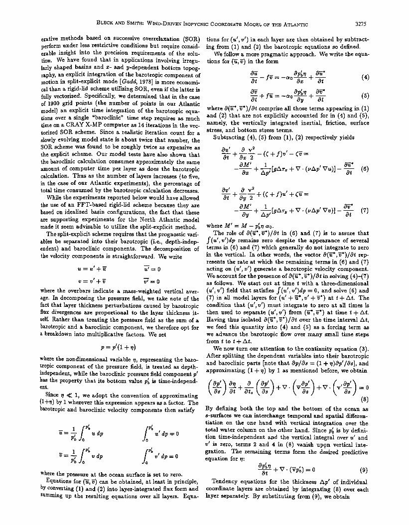
In this section we will demonstrate the numerical proper- ties of the isopycnic model in the simplified case of a rectan- gular ocean basin with an eastward-sloping bottom near the western basin boundary. We use the terms "low-cut" and "high-cut"topography to indicate the extent to which the slope extends up the western sidewall. In the high-cut case, the slope ascends from 4000 m to a depth of 200 m over a horizontal distance of 2000 kin, whereas in the low-cut case it ascends to 1550 m over a distance of 1400 km. We will present results of coarse-resolution (i.e., noneddy-resolving), double-gyre, wind-driven spinup experiments with two and three model layers.

The rectangular ocean basin in these experiments is di- menstoned 4400 km east-west by 6000 km north-south, with uniform grid spacing Az = A y = 200 kin. The vertical structure for the simplest model configuration consists of two layers whose initial thicknesses are 1000 and 3000 m (1000 and 3000 x 10' Pa, to be precise) in the flat-bottom region. The specific volume values in these layers are 0.974 and 0.973 x 10-3m3kg -• , respectively, equivalent to poten- tial density values 26.6 and 27.4. For the three-layer model configuration, the corresponding values are: layer thickness 300, 700, and 3000 m; specific volume 0.975, 0.974, and 0.973 x 10-3m3kg-•; potential density 26.0, 27.0, and 27.7.

The Coriolis parameter varies as f = fo + (y - Y/2)•, where y is the north-south coordinate, Y is the north-south basin size, fo = 0.83 x 10-*s -•, and • = 2 x !0-•m-•s-•. The model is driven by an east-west surface wind stress pat- tern of the form

r•=ro cos [2•r (• -- 1•)] where ro/po • 1.0 x 10-•m•'s -•.

4400 krn

200m I i

o o

Fig. 1. Basin configuration and dimensions. Dashed line indicates "low-cut" shelf configuration.

The horizontal eddy viscosity coefficient •, is set equal to lOOmis -•. No-slip boundary conditions are imposed on all lateral boundaries; the implementation of these conditions along submerged sidewalls is discussed in Appendix C. The low-cut and high-cut bottom topography configurations are illustrated in Figure 1.

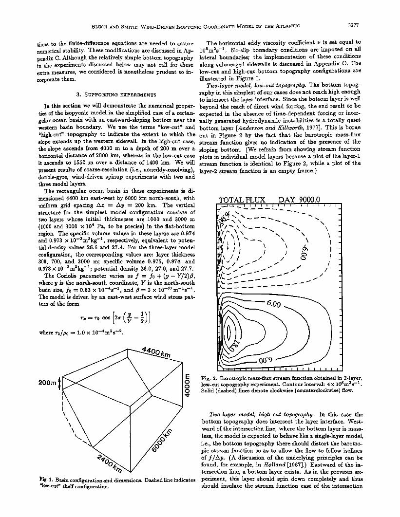
Two-layer model, low-cut topography. The bottom topog- raphy in this simplest of our cases does not reach high enough to intersect the layer interface. Since the bottom layer is well beyond the reach of direct wind forcing, the end result to be expected in the absence of time-dependent forcing or inter- natty generated hydrodynamic instabilities is a totally quiet bottom layer [Anderson and Killworth, 1977]. This is borne out in Figure 2 by the fact that the barotropic mass-flux stream function gives no indication of the presence of the sloping bottom. (We refrain from showing stream function plots in individual model layers because a plot of the layer-1 stream function is identical to Figure 2, while a plot of the layer-2 stream function is an empty fraIne.)

TOTAL FLUX DAY 9000.0

Ir_c;,• 'x --._---- .. -. l

•f/l"' \ x. __. x \ q

'., -,, :

E:;-' ---' -- ,'

6.00

Fig. 2. Barotropic mass-flux stream function obtained in 2-layer, low-cut topography experiment. Contour interval: 4 x 10•m3s -• . sona (dashed) hues denote clockwise (counterclockwise) flow.

Two-layer model, high-cut topography. In titis case the bottom topography does intersect the layer interface. West- ward of the intersection hue, where the bottom layer is mass- less, the model is expected to behave like a single-layer model, i.e., the bottom topography there should distort the barotto- pic stream function so as to allow the flow to follow isolines of flap. (A discussion of the underlying principles can be found, for example, in Holland [1967].) Eastward of the in- tersection line, a bottom layer exists. As in the previous ex- periment, this layer should spin down completely and thus should insulate the stream function east of the intersection

3178 BLECK AND SMITH: WIND-DRIVEN ][SOPYCNIC COORDINATE MODEL oF 'tHE ATLANTIC

TOTAL FLUX DAY 9000.0 [ I / I '1" i I I I I '1 ! i .... !' I I "1' I ! .... I I '1 .....

E //__.. -. - k [ //'•'•"-------. "\

F ,!c•Y///. '" \ x' "' '" . ''\ \\- F x ,, , I -

[-/jIt./' / P: t -

[-I i I \-/ ..--'" •" ../ / - I'-I [ \ -•" _---"' // -

_! •//

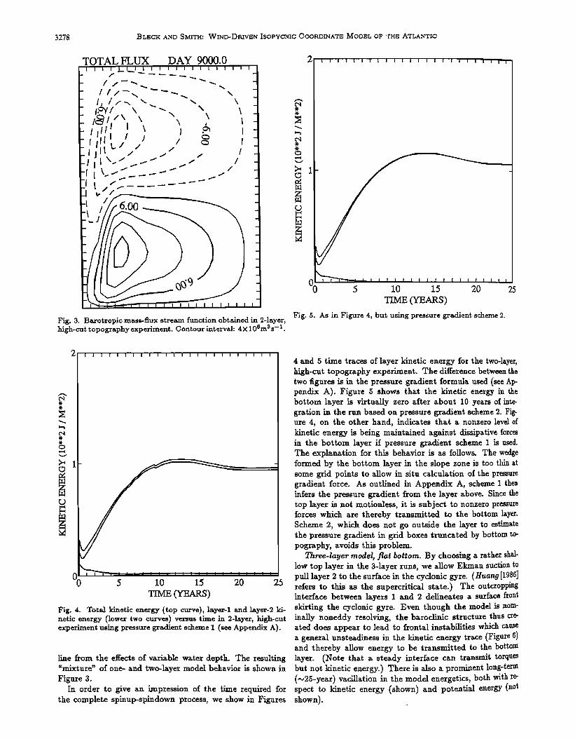
Fig. 3. Baxotropic mass-flux stream function obtained in 2-layer, high-cut topography experiment. Contour interval: 4 X I 0øm3s -1 .

2 i I " '1 ! I I ! I I ! "1 I I ! I I I I I I i i T-

I I I ,i I I I I

20 25

TIME (YEARS)

Fig. 5. As in Figure 4, but using pressure gradient scheme 2.

I I I I I I I'"1 ! I' I I I I I 'I''i ........ I I I 1 I' I I

00 5 10 !5 20 25 TMa (YAS)

Fig. 4. Total kinetic energy (top carve), !ayer-1 and layer-2 ki- netic energy (lower two curves) versus time in 2-layer, high-cut experiment using pressure gradient scheme 1 (see Appendix A).

line from the effects of variable water depth. The resulting "mixture" of one- and two-layer model behavior is shown in Figure 3.

In order to give an impression of the time required for the complete spinup-spindown process, we show in Figures

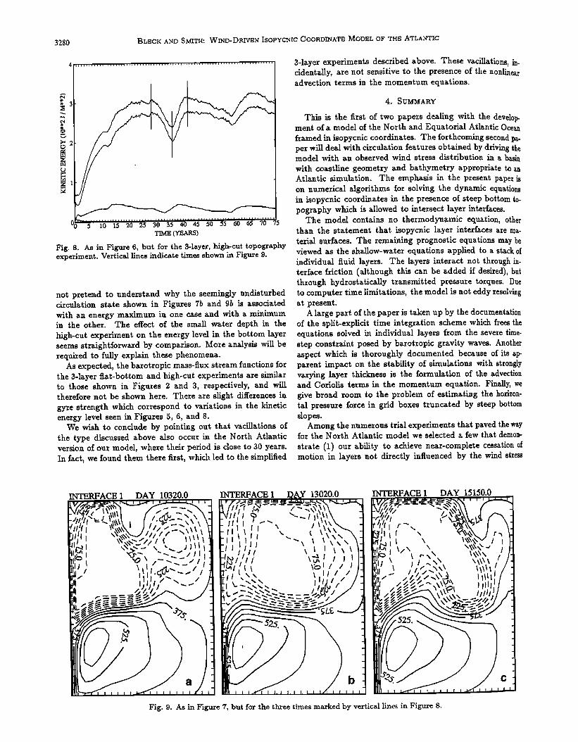
4 and 5 time traces of layer kinetic energy for the two-layer, high-cut topography experiment. The difference between the two figures is in the pressure gradient formula used (see Ap- pendix A). Figure 5 shows that the kinetic energy in the bottom layer is virtually zero after about 10 years of inte- gration in the run based on pressure gradient scheme 2. Fig- ure 4, on the other hand, indicates that a nonzero level of kinetic energy is being maintained against dissipative forces in the bottom layer if pressure gradient scheme ! is used. The explanation for this behavior is as follows. The wedge formed by the bottom layer in the slope zone is too thin at some grid points to allow in situ calculation of the pressure gradient force. As outlined in Appendix A, scheme 1 then infers the pressure gradient from the layer above. Since the top layer is not motionless, it is subject to nonzero pressure forces which are thereby transmitted to the bottom layer. Scheme 2, which does not go outside the layer to estimate the pressure gradient in grid boxes truncated by bottom to- pography, avoids this problem.

Three-laver model, fiat bottom. By choosing a rather shal- low top layer in the 3-layer runs, we allow Ekman suction to pull layer 2 to the surface in the cyclonic gyre. (Huan911986] refers to this as the supercritical state.) The outcropping interface between layers I and 2 delineates a surface front skirting the cyclonic gyre. Even though the model is nora- inally noneddy resolving, the baroclinic structure thus cre- ated does appear to lead to frontal instabilities which cause a general unsteadiness in the kinetic energy trace (Figure 6) and thereby allow energy to be transmitted to the bottom layer. (Note that a steady interface can transmit torques but not kinetic energy.) There is also a prominent long-term (•25-year) vacillation in the model energetics, both with re- spect to kinetic energy (shown) and potential energy (not shown).

BLECK AND SMITH: WIND-DRIVEN ISOP¾CNIC COORDINATE MODEL OF THE; ATLANTIC 3279

4

•3

Oo

ure 7a near the northern basin boundary. This body can be traced back dockwise to the eastern sector of the cy- clonic gyre from which it emerged several years earlier as an identifiable entity. Its source region is characterized by con- siderable long-term variability in the position of the surface front.

The cusp in the kinetic energy curve occurs when the body of layer-1 water is being sucked into the western bound- ary current. Figure 7b shows that the body is hidden from view during that phase. Whether it emerges intact from the boundary current and continues its counterclockwise motion around the cyclonic gyre is difficult to assess. Figure 7c does show a perturbation in the layer thickness isopleths in the southern sector of the anticyclonic gyre at a time when en- ergy returns to its normal level. However, a tracer advection experiment would have to be carried out to establish a clear connection between this rather diffuse thickness anomaly and the far more distinct pool of layer-1 water seen earlier along the northern boundary. Such an experiment could also be

,,,•.,,,. ......... . .................. • ..... used to establish whether remnants of this disturbance, as it 5 l0 15 20 25 •0 35 40"'4•"•'6 '•5•"•'0"•"5'•"55 comes around full circle, trigger the formation oœ a new one

TIME(YEARS) in the eastern part of the cyclonic gyre, or simply a rejuve- Fig. 6. Total kinetic energy (top curve), layer-I, layer-2 and layer- 3 kinetic energy (lower three curves) versus time in 3-layer, flat- bottom experiment. Vertical lines indicate times shown in Figure 7.

We are presently not equipped to analyze the connection, ff one exists, between the relatively short-term energy fluc- tuations and the long-term vacillation visible in Figure 6. It is fairly straightforward, however, to link the 25-year cusps in the kinetic energy curve to a particular event in the evo- lution of the flow field. To illustrate the event, we show in Figure 7 snapshots of layer-/ thickness (plotted as depth of the layer-I/layer-2 interface) at three consecutive times

nation of the old one. Experiments of this type are planned. Three-layer model, hi9h-cut topography. Time traces of

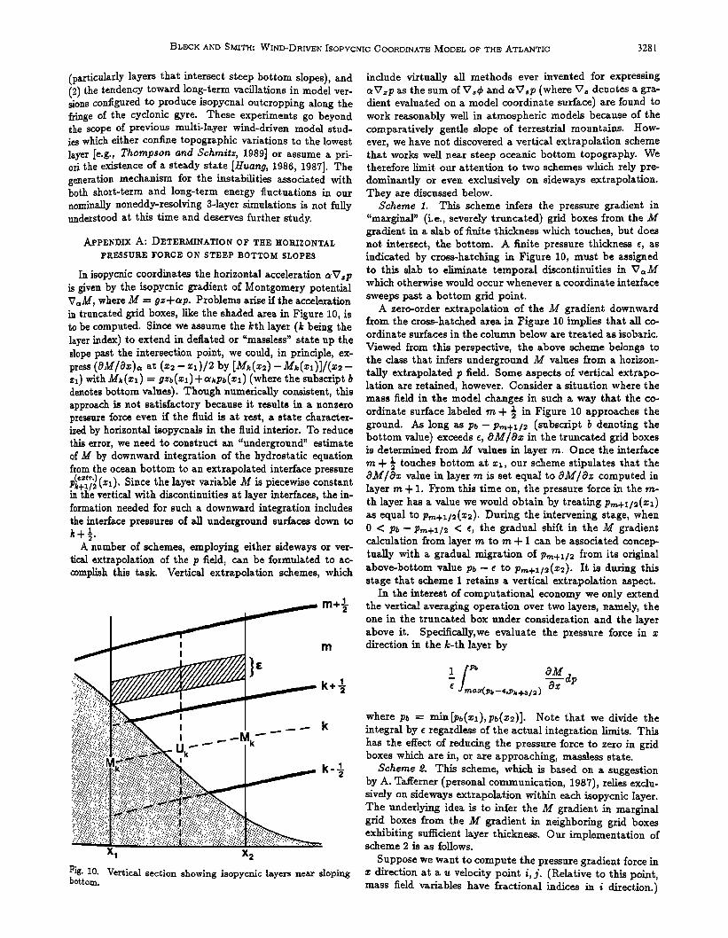
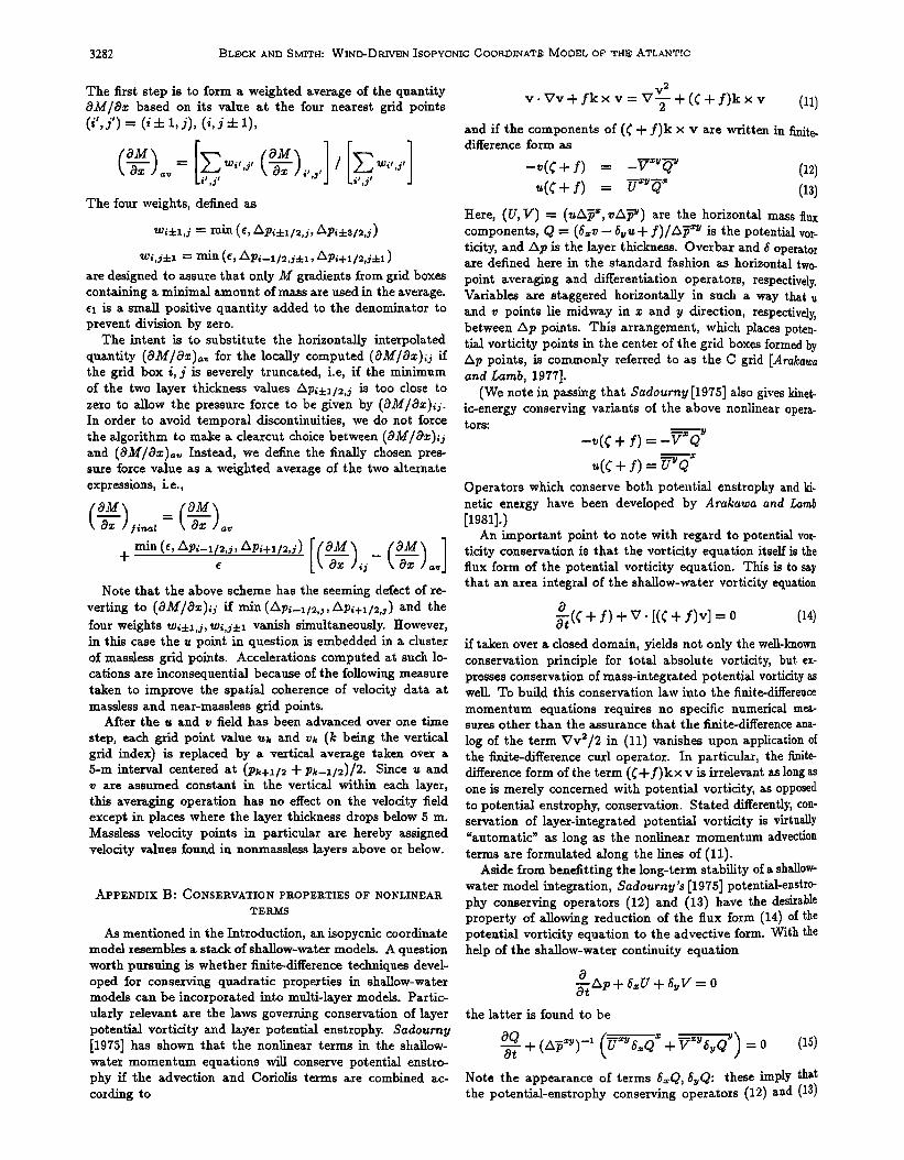
layer kinetic energy for this experiment are shown in Figure 8. Once again, there is a marked 25-year cycle in the en- ergy curves, except that the cusps mark minima, rather than maxima as seen in the flat-bottom case. Figure 6 also differs from Figure 8 in the energy level of the lowest layer. Since most of the kinetic energy in our noneddy-resolving model is found in the western boundary currents, we attribute the differences between Figures 6 and 8 to the small water depth near the western edge. As in the flat-bottom experiment, a cusp in the energy curve occurs every time a body of layer-1 water originating in the eastern part of the cyclonic gyre and

a few years before, at the height of, and a few years after migrating anticlockwise around it gets sucked into the south- the energy peak near year 38 (see Figure 6). The item of ward flowing boundary current. This sequence of events is interest is the isolated body of layer-1 water seen in Fig- shown in Figure 9 which is rather similar to Figure 7. We do

INTERFACE 1 12780.0 INTERFACE 1 DAY 13830.0 INTERFACE 1 DAY 15330.0 '•-•--•--•--• ' x' ''''' r/•-•=•_.=•-•__:•_•-•-•x,,, ,•-•

_

Fig. 7. Depth of the layer-1 lower interface at t•ee times m•ked by vertic• 5nes in Fi•e 6. Sold (d•hed) •nes denote inte•ace depZh •eater (less) th• t•e 300-m depth at time zero. Conto• interv•: 50 m.

375.

3280 BLECK AND SMITH: VV!ND-DRIVEN ISOP¾CNIC COORDINATE MODEL OF THE ATLANTIC

2

TIME (YEARS)

Fig. 8. As in Figure 6, but for the 3-layer, high-cut topography experiment. Vertical lines indicate times shown in Figure 9.

not pretend to understand why the seemingly undisturbed circulation state shown in Figures 75 and 95 is associated with an energy maximum in one case and with a minimum in the other. The effect of the small water depth in the high-cut experiment on the energy level in the bottom layer seems straightforward by comparison. More analysis will be required to fully explain these phenomena.

As expected, the barotropic mass-flux stream functions for the 3-layer fiat-bottom and high-cut experiments are similar to those shown in Figures 2 and 3, respectively, and will therefore not be shown here. There are slight differences in gyre strength which correspond to variations in the kinetic energy level seen in Figures 5, 6, and 8.

We wish to conclude by pointing out that vacillations of the type discussed above also occur in the North Atlantic version of our model, where their period is close to 30 years. In fact, we found them there first, which led to the simplified

3-layer experiments described above. These vacillations, in- cidentally, are not sensitive to the presence of the nonlinear advection terms in the momentum equations.

4. SUMMARY

This is the first of two papers dealing with the develop- ment of a model of the North and Equatorial Atlantic Ocean framed in isopycnic coordinates. The forthcoming second p•. per will deal with circulation features obtained by driving the model with an observed wind stress distribution in a b•sin with coastline geometry and bathymetry appropriate to •n Atlantic simulation. The emphasis in the present paper is on numerical algorithms for solving the dynamic equations in isopycnic coordinates in the presence of steep bottom to- pography which is allowed to intersect layer interfaces.

The model contains no thermodynamic equation, other than the statement that isopycnic layer interfaces are rn•- teria! surfaces. The remaining prognostic equations may be viewed as the shallow-water equations applied to a stack of individual fluid layers. The layers interact not through in- terface friction (although this can be added if desired), but through hydrostatically transmitted pressure torques. Due to computer time limitations, the model is not eddy resolving at present.

A large part of the paper is taken up by the document•ti0n of the split-explicit time integration scheme which frees the equations solved in individual layers from the severe time- step constraint posed by barotropic gravity waves. Another aspect which is thoroughly documented because of its •p- parent impact on the stability of simulations with strongly varying layer thickness is the formulation of the advection and Coriolis terms in the momentum equation. Finally, we give broad room to the problem of estimating the horizon- tal pressure force in grid boxes truncated by steep bottom slopes.

Among the numerous trial experiments that paved the way for the North Atlantic model we selected a few that demon- strate (1) our ability to achieve near-complete cessation of motion in layers not directly influenced by the wind stress

INTERFACE 1 DAY 10320.0

.lf g• I %,,xX,' I/_,/.".-..xx • • u it;,; I' \x :,,x,?_.'///t ! '. • • • .[I

I / "-' '1

I!i"

INTERFACE 1 13020.0

/-..

I• •' -. / ?l ''\, /', \ I i

•x\,, \ I f I I

;œc,.,

b

INTERFACE 1 DAY 15150.0 n •/2f. •. -•u•---•--• • .•----•. • ' ' ' •

Ei. - -'-

- , '1 • •:/ ' • IIIII

Fig. 9. As in Figure 7, but for the three times marked by vertical lines in Figure 8.

BLECK AND SMITH: WIND-DRIVEN ISOPYCNIC COORDINATE MODEL OF THE ATLANTIC 3281

(particularly layers that intersect steep bottom slopes), and (2) the tendency toward long-term vacillations in model ver- sions configured to produce isopycnal outcropping along the fringe of the cyclonic gyre. These experiments go beyond the scope of previous multi-layer wind-driven model stud- ies which either confine topographic variations to the lowest layer [e.g., Thompson and Schmitz, 1989] or assume a pri- ori the existence of a steady state [Huang, 1986, 1987]. The generation mechanism for the instabilities associated with both short-term and long-term energy fluctuations in our nominally noneddy-resolving 3-layer simulations is not fully understood at this time and deserves further study.

APPENDIX A: DETERMINATION OF THE HORIZONTAL PRESSURE FORCE ON STEEP BOTTOM SLOPES

In isopycnic coordinates the horizontal acceleration aVzp is given by the isopycnic gradient of Montgomery potential V•M, where M = gz+ap. Problems arise if the acceleration in truncated grid boxes, like the shaded area in Figure 10, is to be computed. Since we assume the kth layer (k being the ltyer index) to extend in deflated or "massless" state up the slope past the intersection point, we could, in principle, ex-

wih = ) + ) (were denotes bottom values). Though numerically consistent, this approach is not satisfactory because it results in a nonzero pressure force even if the fluid is at rest, a state character- ized by horizontal isopycnals in the fluid interior. To reduce this error, we need to construct an "underground" estimate of M by downward integration of the hydrostatic equation from the ocean bottom to an extrapolated interface pressure

(•xt•) ß . •%+• • (x•) Since the layer variable M is piecewise constant / . in the vertical with discontinuities at layer interfaces, the in- formation needed for such a downward integration includes the interface pressures of all underground surfaces down to

A number of schemes, employing either sideways or ver- tical extrapolation of the p field, can be formulated to ac- complish this task. Vertical extrapolation schemes, which

m+«

k+!

':/. ':'5..".....?ii•

:":):...:.:•ii!? Uk k-•

i•i: % i'. i ':::.,: :)'.':' "•,- '..,?,'•....• :?. :i: !, 'i, ::?:i:{: :'/,:.!•i: !.• :} ::. !:.

'" ' ,

¾:•:',::'.::• x! x 2

Fig. 10. Vertical section showing isopycnic layers near sloping bottom.

include virtually all methods ever invented for expressing c•Vzp as the sum of V• and c•Vsp (witere V• denotes a gra- dient evaluated on a model coordinate surface) are found to work reasonably well in atmospheric models because of the comparatively gentle slope of terrestrial mountains. How- ever, we have not discovered a vertical extrapolation scheme that works well near steep oceanic bottom topography. We therefore limit our attention to two schemes which rely pre- dominantly or even exclusively on sideways extrapolation. They are discussed below.

Scheme 1. This scheme infers the pressure gradient in "marginal" (i.e., severely truncated) grid boxes from the M gradient in a slab of finite thickness which touches, but does not intersect, the bottom. A finite pressure thickness e, as indicated by cross-hatching in Figure 10, must be assigned to this slab to eliminate temporal discontinuities in X7, M which otherwise would occur whenever a coordinate interface

sweeps past a bottom grid point. A zero-order extrapolation of the M gradient downward

from the cross-hatched area in Figure 10 implies that all co- ordinate surfaces in the column below are treated as isobaric.

Viewed from this perspective, the above scheme belongs to the class that infers underground M values from a horizon- tally extrapolated p field. Some aspects of vertical extrapo- lation are retained, however. Consider a situation where the mass field in the model changes in such • way that the co- ordinate surface labeled rn + • in Figure 10 approaches the ground. As long as p•,- P,.,-,+x/2 (subscript b denoting the bottom value) exceeds e, OM/c9x in the truncated grid boxes is determined from M values in layer rn. Once the interface rn + • touches bottom at xx, our scheme stipulates that the OM/Ox value in layer rn is set equal to OM/az computed in layer rn + 1. From this time on, the pressure force in the m- th layer has a value we would obtain by treating p,r,+x/•(xx) as equal to pm+•_/•(z•). During the intervening stage, when 0 < p•,- P,r,+x/• < e, the gradual shift in t}te M gradient calculation from layer rn to rn + 1 can be associated concep- tually with a gradual migration of p,•+x/• from its original above-bottom value pb- ½ to P,r,+x/•(a:2). It is during this stage that scheme 1 retains • vertical extrapolation aspect.

In the interest of computational economy we only extend the vertical averaging operation over two l•yers, namely, the one in the truncated box under consideration and the layer above it. Specifically, we evaluate the pressure force in x direction in the k-th layer by

1_/•• O M dp where i0, = min[p,(z•),pb(z•)]. Note that we divide the integral by ½ regardless of the actual integration limits. This has the effect of reducing the pressure force to zero in grid boxes wlfich are in, or are approaching, massless state.

Scheme œ. This scheme, which is based on a suggestion by A. Tafferner (personal communication, 1987), relies exclu- sively on sideways extrapolation within each isopycnic layer. The underlying idea is to infer the M gradient in marginal grid boxes from the M gradient in neighboring grid boxes exhibiting sufficient layer thickness. Our implementation of scheme 2 is as follows.

Suppose we want to compute the pressure gradient force in a: direction at s u velocity point i, j. (Relative to this point, mass field variables have fractional indices in i direction.)

3282 BLECK AND SMITH: WIND-DI{IVEN ISOPYCNIC COORDINATE MODEL OF THE ATLANTIC

The first step is to form a weighted average of the quantity OM/•z based on its value at the four nearest grid points (i',f) = (iñ •,•), (•,•ñ •),

• = wi,,i, • •',•' / wi,,•, The four weights, defined as

wi4-x,i = min (½, APiq-•12,j', APi4. sl•,j)

are designed to assure that only M gradients from grid boxes containing a minimal amount of mass are used in the average. ex is a sma• positive quantity added to the denominator to prevent division by zero.

The intent is to substitute the horizonta•y interpolated quantity (OM/Ox)• for the locally computed (OM/Oz)i3 if the grid box i, j is severely truncated, i.e, if the minimum of the two layer thi&ness vMaes Apim•/•,3 is too close to ze•o to aHow the pressure force to be given by In order to avoid temporal discontinuities, we do not force the Mgorithm to make a clearcut choice between (OM/Oz)•3 and (OM/Oz)• Instead, we define the finally chosen pres- sure force value as a weighted average of the two a!ternate expressions, i.e.,

final

Note that the above scheme has the seeming defect of re- verting to (•M/Ox)i• if rain (Api_•/a,•.,/Xpi+•/2,•) and the four weights voiñ•,•., wl,jñ• vanish simultaneously. However, in this case the u point in question is embedded in a cluster of massless grid points. Accelerations computed at such lo- cations are inconsequential because of the following measure taken to improve the spatial coherence of velocity data at massless and near-massless grid points.

After the u and v field has been advanced over one time

step, each grid point value u• and va (k being the vertical grid index) is replaced by a vertical average taken over a 5-m interval centered at (10•,+•/a + p•-•/2)/2. Since u and v are assumed constant in the vertical within each layer, this averaging operation has no effect on the velocity field except in places where the layer thickness drops below 5 m. Massless velocity points in particular are hereby assigned velocity values found in nonmassless layers above or below.

APPENDIX B: CONSERVATION PROPERTIES OF NONLINEAR. TERMS

As mentioned in the Introduction, an isopycnic coordinate model resembles a stack of shallow-water models. A question worth pursuing is whether finite-difference techniques devel- oped for conserving quadratic properties in shallow-water models can be incorporated into multi-layer models. Partic- ularly relevant are the laws governing conservation of layer potential vorticity and layer potential enstrophy. $adourny [1975] has shown that the nonlinear terms in the shallow- water momentum equations will conserve potential enstro- phy if the advection and Coriolis terms are combined ac- cording to

v. V'v+ fk x v = X7-• + ((+ f)k x v (11) and if the components of (f + f)k x v are written in finite- difference form as

--v(½ q- f) ---- -Vz"• TM (12) •(½+f) = ¾•U •

tiere, (U, V) = (•a• •, •aF) •re •he horizo.t•l m•ss compo.e•s, • = (•- •. + f)/aF" is •ne po•e.•i• vor- tici%y, •nd Ap is t•e layer t•ickness. Overbar and 5 operator ß re denned here in the standard fashion as horizontal tw• point averaging and differentiation operators, respectively. Variables are staggered horizonta•y in such a way that u and v points !ie midway in z •nd y direction, respectively, between •p points. This arrangement, which places poten- tial vorticity points in the center of the grid boxes formed by •p points, • commonly referred to as the C grid [Arakawa and Lamb, 1977].

(We note in p•ssing that Sadourny [1975] also gives kinet- ic-energy conserving variants of the above nonlinear opera- tors:

-v(C + f) = -•'•

Operators which conserve both potential enstrophy and netic energy have been developed by Arakawa and Lamb

An important point to note with regard to potential vor- ticity conservation is that the vorticity equation itself is the flux form of the potential vorticity equation. This is to say that an area integral of the shallow-water vorticity equation

o•(C + f) + v. [(C + f)v] = 0 (•4) if taken over a closed domain, yields not only the well-known conservation principle for totM •bsolutc vorticity, but ex- presses conservation of mass-integrated potential vorticity as well. To build this conservation law into the finite-difference

momentum equations requires no specific numerical mea- sures other than the assurance that the finite-difference ana-

log of the term Vve/2 in (11) vanishes upon app•cation of the finite-difference curl operator. In particular, the finite- difference form of the term ((+ f)kx v is irrelevant as long as one is merely concerned with potential vorticity, as opposed to potential enstrophy, conservation. Stated differently, con- servation of layer-integrated potential vorticity • virtu•y "automatic" •s long as the nonlinear momentum advection terms •re formulated along the 5nes of (11).

Aside from benefitting the long-term stability of a shadow- water model integration, Sadourny's [1975] potential-enstr• phy co.•e•vin• opemo•s (•2) •nd (•a) h•ve the de•i•Ue property of a•owing reduction of the flux form (14) of the potential vorticity equation to the advective form. With the help of the shadow-water continuity equation

0

the latter is found to be

( a• + (a•)-• • *• + 7 *• = 0 No•e the appearance of terms •Q, •Q: these imply the po•en•iM-enstrophy conserving operators (12) and

BSECK AND SMITH: WIND-DRIVEN ISOPYCNIC COORDINATE MODEL OF THE ATLANTIC 3283

in the momentum equations keep the potential vorticity field constant in regions where it is spatially uniform to begin with. An arbitrarily chosen finite-difference rendition of the flux form (14) of the potential vorticity equation will not necessarily offer this feature, i.e., it will conserve potential vorticity only in the layer-integrated sense.

The appearance of the variable Q in (12) and (13)in- dicates tha• potential enstrophy conserving operators can only be used if the minimum thickness of individual coor- dinate layers is nonzero at all times. In a general-purpose circulation model allowing isopycnMs to intersect the sea sur- face and the bottom topography, this condition is clearly not satisfied. Fortunately, this does not close the door on •1l •ttempts to use potentiM-enstrophy conserving finite-dif- ference operators. There are various ways to "shield" the finite-difference equations in the oceanic interior, where layer •hickness remains finite, from the detrimental effects of zero layer thickness. We will describe here one possible modifica- tion to the enstrophy-conserving scheme (12) and (in) which allows it to revert smoothly to a more robust finite-difference expression wherever the denominator in the expression for Q is about to reach zero.

The numerical overflow occurring in the calculation of Q is only one aspect of the problem posed by vanishing layer thickness. Another aspect, and perhaps a physically more relevant one, is that the layer integral of squared, mass- weighted potential vorticity (i.e., the potential enstrophy in the layer) may be infinite if layer depth varies gradually be- tween zero and nonzero values. An infinite reservoir of po- tential enstrophy clearly makes potential enstrophy conser- vation useless as a guarantor of long-term numerical stability. We may also expect the unbounded and poorly resolved gra- dient of Q in the transition zone between zero and non-zero layer thickness to push the truncation and phase errors in the Q advection equation (15) far beyond acceptable limits.

In light of these problems, it seems inadvisable to rely on (•2) and (•3) when solving the momentum equation in a zone where the layer depth gradually approaches zero. The proper fall-back position is to require that the expressions (12) and (13) revert to a form of (( + f)k x v not involving layer thickness. Our procedure for accomplishing this is as follows.

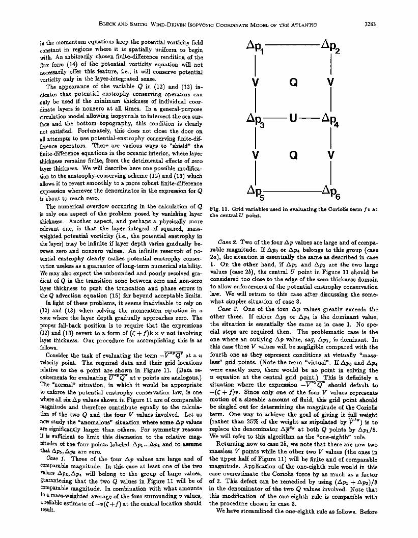
Consider the task of evaluating the term --••'• at a u velocity point. The required data and their grid locations relative to the u point are shown in Figure !1. (Data re- quirements for evaluating •xy•x at v points are analogous.) The "normal" situation, in which it would be appropriate to enforce the potential enstrophy conservation law, is one where all six Ap values shown in Figure 11 are of comparable magnitude and therefore contribute equally to the calcula- tion of the two Q and the four V values involved. Let us now study the "anomalous" situation where some Ap values are significantly larger than others. For symmetry reasons it is sufficient to limit this discussion to the relative mag- nitudes of the four points labeled Api...Ap4 and to assume that Aps, Ape are zero.

Case !. Three of the four Ap values are large and of comparable magnitude. In this case at least one of the two values Aps, Ap4 will belong to the group of large va!ues, guaranteeing that the two Q values in Figure 11 will be of comparable magnitude. In combination with what amounts to a mass-weighted average of the four surrounding v values, • reliable estimate of-v(½ + f) at the central location should result.

V Q V

,U

v Q v

Fig. 11. Grid variables used in evaluating the Coriolis term fv at the central U point.

Case 2. Two of the four Ap values are large and of compa- rable magnitude. If Ap3 or Ap4 belongs to this group (case 2a), the situation is essentially the same as described in case !. On the other hand, if Apl and Ap•. are the two large values (case 2b), the central U point in Figure !1 should be considered too close to the edge of the zero thickness domain to allow enforcement of the potential enstrophy conservation law. We will return to this case after discussing the some- what simpler situation of case 3.

Case 3. One of the four /Xp values great!y exceeds the other three. If either Apa or Ap4 is the dominant value, the situation is essentially the same as in case 1. No spe- cial steps are required then. The problematic case is the one where an outlying Ap value, say, Z•px, is dominant. In this case three V values will be negligible compared with the fourth one as they represent conditions at virtually "mass- less" grid points. (Note the term "virtuM". If ZXpa and Ap, were exactly zero, there would be no point in solving the u equation at the central grid point.) This is definitely situation where the expression -V Q should default to -(½ + f)v. Since only one of the four V values represents motion of a sizeable amount of fluid, this grid point should be singled out for determining the magnitude of the Coriolis term. One way to achieve the goal of giving it full weight (rather than 25% of the weight as stipulated by •x•)is to replace the denominator A• xy at both Q points by Ap•/8. We will refer to this algorithm as the "one-eighth" rule.

Returning now to case 2b, we note that there are now two massless V points while the other two V values (the ones in the upper half of Figure 11) will be finite and of comparable magnitude. Application of the one-eighth rule would in this case overestimate the Coriolis force by as much as a factor of 2. This defect can be remedied by using (Apx in the denominator of the two Q values involved. Note that this modification of the one-eighth rule is compatible with the procedure chosen in case 3.

We have streamlined the one-eighth rule as follows. Before

3284 BLECK AND SMITH: WIND-DRIVEN ISOPYCNIC COORDINATE MODEL OF THE ATLANTIC

computing the Q field we determine in each grid square the sum of the two largest Ap corner values; we shall denote this sum by I!ij (i, j being the grid indices). The denominator in Qij is then given the value

max (Hi.i, !Ii-•,j, IIi+•.,j, IIi,./-•., IIi,j+•. ) (•6)

If both alternatives are zero, all possible V•"• and combinations involving Qij will be comprised of zero Us and

where the index i varies in z direction and the subscript "bot" denotes bottom pressure.

A lateral drag condition (free-slip or no-slip) is applied to flow tangent to submerged orographic obstacles. R, ecM1 that lateral drag is incorporated in the momentum equations (1) and (2) through the eddy momentum flux •,/XpVv. Consider the exchange of u-momentum in y direction between two grid

Vs; in •his case there is no need •o solve the momentum boxes, (i,j) and (/,j-l) (•bbreviated here as j and j-l). If equations in the vicinity of grid point i, j because we are too point j is

• boundary conditions are invoked by setting far from grid points containing actual mass. An arbitrary nonzero value in the denominator of Q may be used in this at j - • to uj - •ruj, witere •r = 1 for free-slip and •r = -1 case to prevent overflow. for no-slip conditions.

The one-eighth rule guarantees that layer potential en- If a "partial" sidewall is present in the form of a seaflo0r atrophy will be conserved as long as Ap within octagonal rise between j and j- 1, the above drag condition is gener- clusters of 12 grid points varies by no more than a factor of Mized by writing four. This fact can be used to prove numerical consistency of the scheme (16): as grid resolution increases and the grid points in Figure 11 migrate toward each other, the spatial variation in the Ap field will eventually fall below the factor- of-four threshold. The scheme then reverts to (12) and (13), whose numerical consistency properties are obvious.

While we have tried to take into account as many config- urations of the Ap field as possible, the one-eighth rule does not guarantee optimal results under all conditions. However, it does satisfy two ixnportant criteria: it avoids (1) compli- cated decision-making algorithms and (2) temporal discon- tinuities in the Q field.

APPENDIX C: KINEMATIC EFFECTS OF STEEP BOTTOM SLOPES

The continental shelf in an oceanic basin inhibits l•teral displacement of abyssal water in a m•nner similar to a ver- tical sidewall. In a model that allows all isopycnic layers to extend to the actual shoreline (where the water depth may only be a few tens of meters) the kinematic boundary conditions posed at the coast clearly are relevant only for near-surface water. Some additional boundary conditions expressing the blocking and lateral drag effect of steep bot- tom slopes are therefore required. One of the most serious problems encountered in the absence of blocking constraints is the occasional extrusion of abyssM water into grid boxes located on the shelf. Depending on the three-dimensionM configuration of the bottom topography, katabatic accelera- tions resulting from these extrusions can lead to numerical instabilities; these appear to be related in part to the need for spatial averaging of the velocity field in the Coriolis term.

The blocking technique we have adopted is reminiscent of the Geophysical Fluid Dynamics Laboratory (GFDL) model "step" mountain. Rather than assuming that the water depth varies linearly between adjacent mass field grid points, we treat the bottom within each mass field grid box as fiat. Thus a "sill" is defined on the boundary between two adja- cent grid boxes that have different water depth. The depth of the flow over the sill is then given by the minimum (as opposed to the average) of the water depths in the upstream and downstream box. The pressure on interior interfaces at u and v points, however, is still given by •x and •v, respec- tively• provided these values do not exceed the sill depth as defined above. To summarize, the depth of the kth interface at, say, a u velocity point labeled i, j is given by

where the aspect ratio •, 0 _< • _< 1 indicates the extent to which the seafloor elevation at j- 1 creates a sidewall if viewed from grid box j.

The vectorized code for implementation of sidewall fric- tion has been found to account for roughly 6% of the total computation time for a 2-layer model experiment.

Acknowledgments. Support for tiffs work by the National Sci- ence Foundation under grants OCE-8600593 and 0CE-8812185 is gratefully acknowledged. Most corni>uœations were carried out at the National Center for Atmospheric Reseaxch, sponsored by the National Science Foundation. Compuœer time was also made available in 1985 by the Geophysical Fluid Dynamics Laboratory, Princeton. Our work benefitted from the strong interest of Dou- glas B. Boudra (deceased) and Claes Rooth at the University of Miami.

REFERENCES

Anderson, D. L. T., and P. D. Killworth, Spin-up of a stratified ocean with topography, Deep Sea Res., 2.4, 709-732, 1977.

Arakawa, A., and V. R. Lamb, Computational design of the ba- sic processes of the UCLA general circulation model, Methods C'omput. _Phys., i 7, !74-265, 1977.

Arakawa, A., and V. R. Lamb A potential enstrophy-and energy- conserving scheme for the shallow water equations, Mort. Wea- ther Rev., 109, 18-36, 1981.

Bleck, R., Finite difference equations in generalized vertical co- ordinates, I, Total energy conservation, Contrib. Aimosph. Phys., 51,360-372, 1978.

B!eck, R., and D. B. Boudra, Initial testing of a numerical ocean circulation model using a hybrid (quasi-isopycnic) vertical co- ordinate, J. Phys. Oceanogr., 11, 7'55-770, 1981.

Bleck, R., and D. B. Boudra, Wind-driven spin-up in eddy-resolv- ing ocean models formulated in isopycnic and isobaric coordi- nates, J. Geophys. Res., 91C, 7611-7621, 1986.

Bleck, R., H. P. Hanson, D. Hu, and E. B. Kraus, Mixed layer- thermocline interaction in a t]:n'ee-dimensional isopycrdc coor- dinate model, J. Phys. Oceano#r., 19, 1417-1439, 1989.

Bryan, K., A numerical method for the study of the circulation of the world ocean, J. Cornput. Phys., .4, 347-376, 1969.

Gadd, A. J., A split-explicit integration scheme for numerical weather prediction, Q. J. R. MeteoroL $oc., 10.4, 569-582, 1978.

Holland, W. R., On the wind-driven circulation in art ocean with bottom topography, Tellus, 19, 582-599, 1967.

Huang, FL. X., Numerical simulation of wind-driven circulationin

BLECK AND SMITH: WIND-DRIVEN ISOPYCNIC COORDINATE MODEL OF THE ATLANTIC 3285

a subtropical/subpolar basin, J. Phys. Oceanoõr., 16, 1636- 1650, 1986.

Huang, R. X., A three-layer model for wind-driven circulation in a subtropical/subpolar basin, I, Model formulation and the subcritical state, o r. Phys. Oceano#r., 17, 664-678, 1987.

Luyten, J. Ft., J. Pedlosky, and H. Storereel, The ventilated ther- toocline, J. Phys. Oceanogr., 13, 292-309, 1983.

Mesinger, F., On the convergence and error problems of the calcu- lation of the pressure gradient force in sigma coordinate models, Geophys. Astrophys. Fluid Dyn., 19, 105-117, 1982.

Montgomery, R. B., Circulation in upper layers of southern North Atlantic deduced with use of isentropic analysis, in Papers in Phys. Oceano#r. and Meteorol., VoL VI, 55 pp., Woods Hole Oceanogr. Inst., Woods Hole, Mass., 1938.

Parsons, A. T., A two-layer model of Gulf Stream separation, J. Fluid Mech., 39, 511-528, 1969.

Sadourny, R., The dynamics of finite-difference models of the shallow-water equations, J. Aimos. Sci., 32, 680-689, 1975.

Thompson, J. D., and W. J. Schmitz, Jr., A limited-areamodel of the Gulf Stream: Design, initial experiments, and model-data intercomparison, J. Phys. Ocear, ogr., 19• 791-814, 1989.

Welander, P., A two-layer frictional model of wind-driven motion in a rectangular oceanic basin, Tellus, 18, 54-.62, 1966.

Zalesak, S., Fully multidimensional flux-corrected transport algo- rithms for fluids, J. Comput. Phys., 31,335-362, 1979.

R. Bleck and L. T. Smith, Rosenstiel School of Marine and Atmospheric Sciences, University of Miaxrd, 4600 Ftickenbacker Causeway, Miami, FL 33149.

(Received May 30, 1989; revised August 30, 1989;

accepted September 5, 1989.)