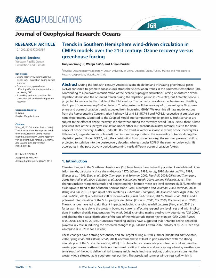
RESEARCH ARTICLE10.1002/2013JC009589

Trends in Southern Hemisphere wind-driven circulation inCMIP5 models over the 21st century: Ozone recovery versusgreenhouse forcingGuojian Wang1,2, Wenju Cai1,2, and Ariaan Purich2

1Physical Oceanography Laboratory, Ocean University of China, Qingdao, China, 2CSIRO Marine and AtmosphericResearch, Aspendale, Victoria, Australia

Abstract During the late 20th century, Antarctic ozone depletion and increasing greenhouse gases(GHGs) conspired to generate conspicuous atmospheric circulation trends in the Southern Hemisphere (SH),contributing to a poleward intensification of the oceanic supergyre circulation. Forcing of Antarctic ozonedepletion dominated the observed trends during the depletion period (1979–2005), but Antarctic ozone isprojected to recover by the middle of the 21st century. The recovery provides a mechanism for offsettingthe impact from increasing GHG emissions. To what extent will the recovery of ozone mitigate SH atmos-phere and ocean circulation trends expected from increasing GHGs? We examine climate model outputfrom the Representative Concentration Pathway 4.5 and 8.5 (RCP4.5 and RCP8.5, respectively) emission sce-nario experiments, submitted to the Coupled Model Intercomparison Project phase 5. Both scenarios aresubject to the effect of ozone recovery. We show that during the recovery period (2006–2045), there is littlepoleward shift of the supergyre circulation under either RCP scenario in austral summer, due to the domi-nance of ozone recovery. Further, under RCP8.5 the trend in winter, a season in which ozone recovery haslittle impact, is greater (more poleward) than in summer, opposite to the seasonality of trends during thedepletion period. Under RCP4.5, with the contribution from ozone recovery, the summer poleward shift isprojected to stabilize into the postrecovery decades, whereas under RCP8.5, the summer poleward shiftaccelerates in the postrecovery period, presenting vastly different ocean circulation futures.

1. Introduction

Climate changes in the Southern Hemisphere (SH) have been characterized by a suite of well-defined circu-lation trends, particularly since the mid-to-late 1970s [Kidson, 1988; Karoly, 1990; Randel and Wu, 1999;Waugh et al., 1999; Zhou et al., 2000; Thompson and Solomon, 2002; Marshall, 2003; Gillett and Thompson,2003; Marshall et al., 2004; Solomon et al., 2006; Roscoe and Haigh, 2007; Lee and Feldstein, 2013]. Thechanges include rising midlatitude and decreasing high-latitude mean sea level pressure (MSLP), manifestedas an upward trend of the Southern Annular Mode (SAM) [Thompson and Solomon, 2002; Marshall, 2003;Wang and Cai, 2013], a spin-up of polar westerlies [Gillett and Thompson, 2003; Roscoe and Haigh, 2007; Leeand Feldstein, 2013], a poleward shift of storm tracks [Scheff and Frierson, 2012b, Barnes et al., 2013], and apoleward intensification of the SH supergyre circulation [Cai et al., 2003; Cai, 2006; Roemmich et al., 2007].These changes have led to significant impacts, including changing rainfall patterns [Kang et al., 2011], afaster warming rate along the western boundary currents affecting regional sea level rises and with implica-tions in carbon dioxide sequestration [Wu et al., 2012], changing marine biodiversity boundaries [Cai, 2006],and altering the spatial distribution of the rate of the midlatitude ocean heat storage [Gille, 2008; Russellet al., 2006; Cai et al., 2010b]. Numerous modeling studies have suggested that Antarctic ozone depletionplayed a key role in inducing the observed changes [e.g., Cai and Cowan, 2007; Polvani et al., 2011; see alsoThompson et al., 2011 for a review].

These changes have a strong seasonality and are largest during austral summer [Thompson and Solomon,2002; Eyring et al., 2013; Barnes et al., 2013], a feature that is at least in part associated with the strongannual cycle of the SH circulation [Cai, 2006]. The characteristic seasonal cycle is from austral autumn thewesterly jet moves northward to its northernmost position in winter and early spring, allowing weather sys-tems south of the jet to deliver rainfall to many midlatitude landmass regions; during austral summer, thewesterly jet is situated at its southernmost position. The associated summer wind-stress curl, which is

Special Section:Western Pacific OceanCirculation and Climate

Key Points:� Ozone recovery will dominate the

trends in SH circulation during australsummer� Ozone recovery provides an

offsetting effect to the impact due toincreasing GHG� A masking period of stabilized SH

circulation will emerge during ozonerecovery

Correspondence to:G. Wang,Guojian.Wang@csiro.au

Citation:Wang, G., W. Cai, and A. Purich (2014),Trends in Southern Hemisphere wind-driven circulation in CMIP5 modelsover the 21st century: Ozone recoveryversus greenhouse forcing, J. Geophys.Res. Oceans, 119, doi:10.1002/2013JC009589.

Received 7 NOV 2013

Accepted 23 APR 2014

Accepted article online 28 APR 2014

WANG ET AL. VC 2014. American Geophysical Union. All Rights Reserved. 1

Journal of Geophysical Research: Oceans

PUBLICATIONS

stronger than that in winter [Cai and Cowan 2007], drives a strong SH supergyre circulation that links thesubtropical gyres of the Atlantic, Indian, and Pacific Oceans (Figure 1). The supergyre circulation, inferredfrom Godfrey’s Island Rule model [Godfrey, 1989], has a strong East Australia Current passing through theTasman Sea with a Tasman leakage from the southern Pacific Ocean to the southern Indian Ocean [Ridgwayand Dunn, 2007], and a similarly strong Agulhas leakage from the southern Indian Ocean to the southernAtlantic Ocean. The closer proximity of the austral summer midlatitude jets and the supergyre circulation tothe high latitudes and the Antarctic means that the supergyre is more influenced by Antarctic ozone deple-tion in summer, even if the impact from ozone depletion were the same across all seasons.

However, the impact by ozone depletion, per se, has a strong seasonality as well. Although the depletionand the resultant circulation changes in the stratosphere are greatest in austral spring [Randel and Wu,1999; Waugh et al., 1999; Zhou et al., 2000; Thompson and Solomon, 2002; Gillett and Thompson, 2003; Pol-vani et al., 2011], because of a delay of a few months for the stratospheric signal to reach the surface, ozonedepletion-induced changes near the surface are largest in summer, coinciding with the season when the SHocean circulation is strong and furthest to the south. As Antarctic ozone recovers, its effect will mitigate theimpact of increasing greenhouse gases (GHGs) [e.g., Arblaster et al., 2011; Wilcox et al., 2012; Barnes et al.,2013]. Understanding this synchronization of the trends with the seasonal maximum of the SH ocean circu-lation is important in the context of the present study, because the mitigating effect from the recovery ofozone on the increasing greenhouse gas-induced trends will also be largest in austral summer.

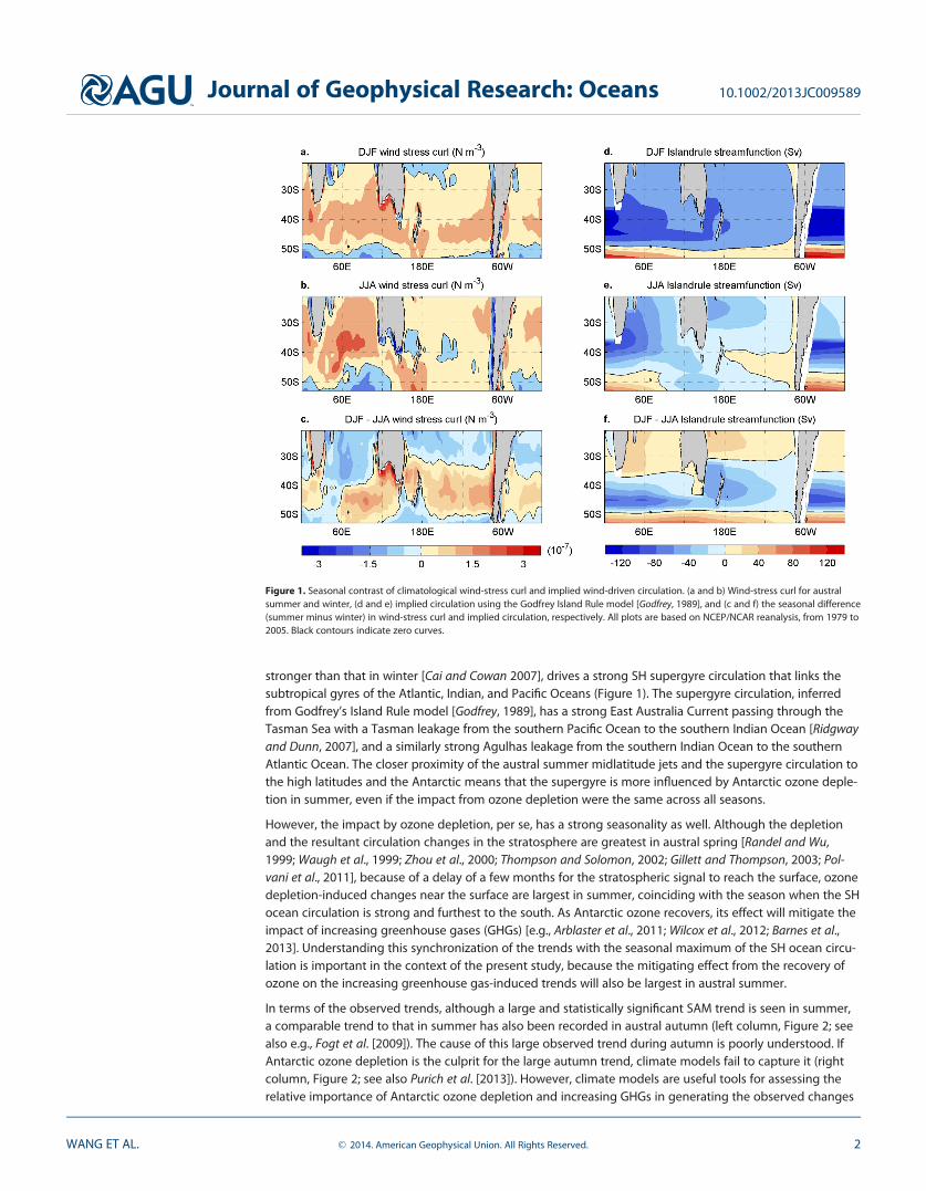
In terms of the observed trends, although a large and statistically significant SAM trend is seen in summer,a comparable trend to that in summer has also been recorded in austral autumn (left column, Figure 2; seealso e.g., Fogt et al. [2009]). The cause of this large observed trend during autumn is poorly understood. IfAntarctic ozone depletion is the culprit for the large autumn trend, climate models fail to capture it (rightcolumn, Figure 2; see also Purich et al. [2013]). However, climate models are useful tools for assessing therelative importance of Antarctic ozone depletion and increasing GHGs in generating the observed changes

Figure 1. Seasonal contrast of climatological wind-stress curl and implied wind-driven circulation. (a and b) Wind-stress curl for australsummer and winter, (d and e) implied circulation using the Godfrey Island Rule model [Godfrey, 1989], and (c and f) the seasonal difference(summer minus winter) in wind-stress curl and implied circulation, respectively. All plots are based on NCEP/NCAR reanalysis, from 1979 to2005. Black contours indicate zero curves.

Journal of Geophysical Research: Oceans 10.1002/2013JC009589

WANG ET AL. VC 2014. American Geophysical Union. All Rights Reserved. 2

[Carril et al., 2005; Miller et al., 2006; Cai and Cowan, 2007]. During phase 3 of the Coupled Model Intercom-parison Project (CMIP3), two groups of climate experiments were carried out, one with ozone depletion andone without, such that a comparison could be made and the role of ozone depletion realized [Cai andCowan, 2007; Son et al., 2008a, 2009; Miller et al., 2006; Purich and Son 2012]. Similar experiments are notavailable from the newly completed CMIP5 experiments. However, for an almost identical ozone recoveryscenario, several GHG emission scenarios are used, allowing an examination of how Antarctic ozone recov-ery can alter future climate under different GHG emission scenarios. As such, this is the mandate of the pres-ent study. A recent study has shown that the position of the SH extratropical jet stream, subtropical dryzone, and sea ice concentration all experience the mitigating effect of ozone recovery [Barnes et al., 2013].Here we complement their findings by first examining the mitigating effect of ozone recovery on the wind-stress curl trend and the associated ocean circulation, and then attempt to quantify the impact.

2. Data and Methods

Although our focus is on the summer season, to highlight the strong seasonality of the impacts from ozonedepletion and recovery, we examine trends in observations and CMIP5 models in all four austral seasons:summer (December, January, February; DJF), autumn (March, April, May; MAM), winter (June, July, August;JJA), and spring (September, October, November; SON). Zonal and meridional wind stress and MSLP aretaken from the National Centers for Environmental Prediction/National Center for Atmospheric Research(NCEP/NCAR) reanalysis [Kalnay et al., 1996]. However, it is known that spurious trends exist in the NCEP/NCAR reanalysis at southern high latitudes [Marshall, 2003] before the late 1970s. For this reason, trends inthe observational period are calculated using data since 1979, when satellite data became available.

Figure 2. Seasonal contrast of wind-stress curl trends during the ozone depletion period of 1979–2005. (a–d) Based on NCEP/NCAR reanal-ysis, and indicate changes in austral summer, autumn, winter, and spring, respectively. (e–h) Same as Figures 2a–2d, but based on a multi-model ensemble average from CMIP5 historical simulations. The red (blue) stippled areas indicate positive (negative) values which aresignificant at the 95% confidence level using a Student’s t-test. Black contours indicate zero curves.

Journal of Geophysical Research: Oceans 10.1002/2013JC009589

WANG ET AL. VC 2014. American Geophysical Union. All Rights Reserved. 3

We utilize outputs from the CMIP5 models under historical and future emission scenarios. The future emis-sion scenarios branch off from historical experiments at the end of 2005 and continue to 2100 under twodifferent Representative Concentration Pathways (RCP) of anthropogenic GHG emissions [Meinshausenet al., 2011]: RCP4.5 (medium-low emission scenario) and RCP8.5 (high emission scenario). To be consistentand to enable a comparison of the results, we use 13 models from which the required variables from bothRCP scenarios are available (ACCESS1-0, ACCESS1-3, CanESM2, CNRM-CM5, CSIRO-Mk3-6-0, GFDL-CM3, GISS-E2-R, HadGEM2-CC, HadGEM2-ES, MIROC-ESM, MIROC-ESM-CHEM, MRI-CGCM3, NorESM1-M). Although multi-ple realizations may exist for the listed 13 models, we only use the first to ensure that all models are equallyrepresented; see Taylor et al. [2012] for CMIP5 experiment information. In RCP8.5, emissions continuethroughout the period and the radiative forcing reaches 8.5 W m22 by 2100. In RCP4.5, emissions areweaker and level off around 2075 to 40% their 2005–2050 rate, and the radiative forcing reaches 4.5 W m22

by 2100. In both RCPs, there is little difference in the magnitude or timing of stratospheric ozone changes,therefore the two RCPs allow an assessment of the relative importance of ozone recovery in the future cli-mate. Given the different emission scenarios, commonality in the characteristics of the future climate in thetwo RCPs could be used to identify the effect of ozone recovery, without which we may expect more sub-stantial differences.

The impact of ozone depletion is generally implemented by prescribing the observed and projected profile ofozone content (height and latitude profile, with temporal evolution), to realize its radiative effect. Becauseozone absorbs solar radiation, a depletion leads to a cooling in the stratosphere, which in turns, alters temper-ature gradients, and hence atmospheric circulation. Some models incorporate an interactive ozone chemistrymodel; in such a way, ozone content is a function of the evolving circulation (example, background tempera-ture and sunlight), instead of a prescribed profile. For each model, we construct a time series of zonal meanzero-curl latitude. A linear fit is applied to the ensemble average in three separated periods similar to Barneset al. [2013]: ozone depletion (1961–2005), recovery (2006–2045), and postrecovery (2046–2100). The lengthof the depletion period here is different from that in Barnes et al. [2013]; while they focus on 1970–2005, forour study a longer period is preferred to assess the inferred ocean circulation change. Although the exact year(2045) for the completion of the recovery is not clearly defined, particularly in models with interactive chemis-try, sensitivity tests show the trend is not sensitive to the choice of end year. Linear trends of grid point wind-stress curl are also calculated to examine the spatial pattern and the implied ocean circulation.

As discussed in the introduction, the models simulate maximum trends of wind-stress curl in australsummer and minimum trends in winter (Figures 2e and 2g), and the simulated positive curl anomalies inwinter are situated equatorward compared with those in summer (Figure 2), similar to CMIP3 model results[Cai and Cowan, 2007]. Thus, not only does the total wind-stress curl field display a distinctive seasonality,the pattern of the trends also possesses a strong seasonality.

Although a trend of wind-stress curl comparable in magnitude to the summer trend is observed during aus-tral autumn, such a trend is not simulated by the models (Figures 2b and 2f). Furthermore, the CMIP5 multi-model average shows several other differences from the observed: the models show a broader region ofstatistically significant wind-stress curl trends in summer, in contrast to the observed (Figures 2a and 2e);the trend pattern is more zonally symmetric than the observed; and multimodel averaged trends in summerare weaker in magnitude (generally only about 50% of the observed). Many of these differences are likely atleast in part a result of the multimodel averaging procedure. In addition, these features suggest that someof the observed changes may have been induced by internal variability, which has been by and largeremoved in the process of our multimodel ensemble average. As in previous studies, the well-definedzonally symmetric feature reflects the fact that much of the trends are congruent with an observed upwardtrend of the SAM [e.g., Cai and Cowan, 2007]. However, the key point here is that during the depletionperiod, the largest impact occurs in austral summer and the smallest in austral winter. Therefore, we expectthe mitigating effect of ozone recovery will also be largest in summer. As such, we will focus on summer inour discussion, but will also maintain a comparison between winter and summer, wherever appropriate.

3. Mitigating Effect of Ozone Recovery on Wind-Stress Curl

We focus on the properties of wind-stress curl in austral summer to provide a depiction of the mitigatingeffect of ozone recovery on the SH supergyre circulation. One of the important parameters that characterize

Journal of Geophysical Research: Oceans 10.1002/2013JC009589

WANG ET AL. VC 2014. American Geophysical Union. All Rights Reserved. 4

changes in the supergyre circulation is the trend of the wind-stress curl magnitude. This has previouslybeen used to study the impact of ozone depletion on ocean circulation [e.g., Cai, 2006]. In the SH, a positivewind-stress curl trend implies an intensification of the gyre. Another important parameter is the zero-curlcurve, which separates the subtropical gyre circulation from the Antarctic Circumpolar Current. This curvedoes not intersect the basin boundaries of Australia or South Africa, but does for South America. This allowsoceanic gyres in the three basins to be linked (for example through the Tasman and Agulhas leakages),transporting water westward from the Pacific Ocean to the Indian Ocean, and from the Indian Ocean to theAtlantic Ocean, respectively [Cai, 2006]. A time series of the zonal-mean latitude of the zero-curl curve (indegrees latitude, where negative values indicates to the south) provides a good indicator of the position ofthe supergyre circulation, although is not perfect for indicating the separation of the subtropical gyres fromthe Antarctic Circumpolar Current (ACC) [De Boer et al., 2013], because of factors such as the presence of abuoyancy-driven forcing. This is calculated for both observations and models using zonal and meridionalwind stress and we assess the evolution of the zonal-mean latitude of the zero-curl curve.

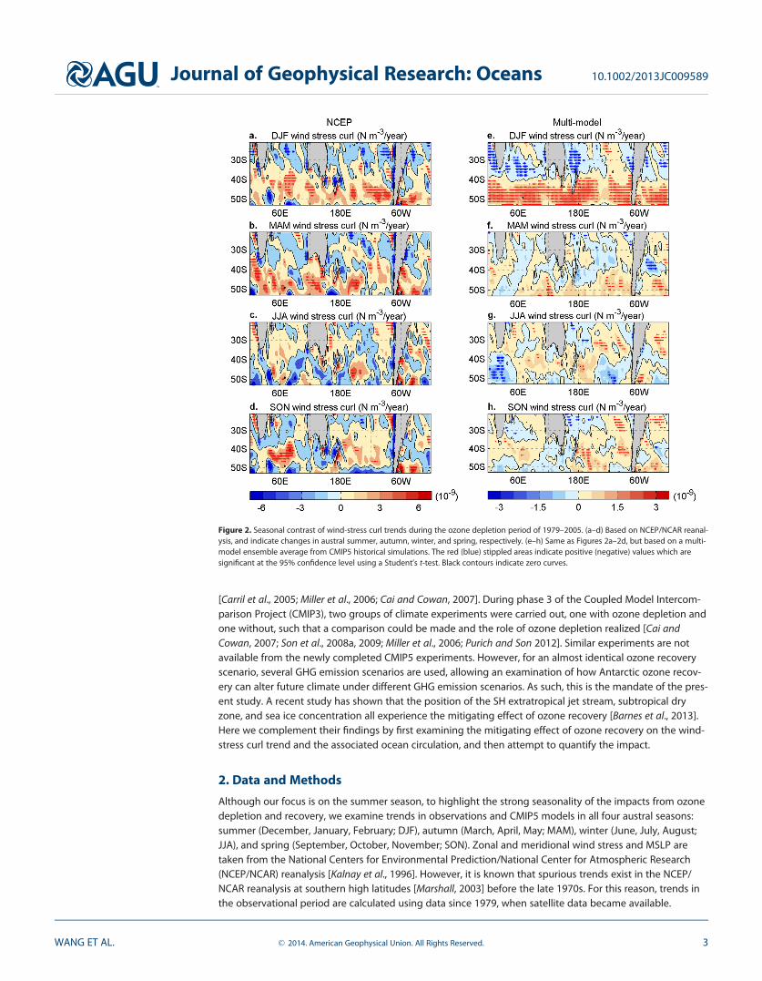
The presence of a mitigating effect from the ozone recovery can be seen from a change in the zonal-meanlatitude of the zero-curl curve. In Figure 3, a linear regression line is constructed for the depletion (1961–2005), recovery (2006–2045), and postrecovery (2046–2100) periods using the multimodel averaged timeseries of the zonal-mean latitude of the zero-curl curve, similar to Barnes et al. [2013]. In summer, the miti-gating effect of the ozone recovery over the 2006–2045 period is evidenced by a strong trend reductionfrom the depletion to the recovery period (Figures 3a and 3b). Given that GHGs continue to increase overboth of these periods, a plausible forcing factor that could generate such a trend reduction in the SH isindeed stratospheric ozone recovery. The trend reduction therefore strengthens the notion of a mitigating

Figure 3. Time series of multimodel zonally averaged austral-summer zero-curl latitude (in degrees latitude: a more negative value indi-cates further to the south). The time series from 1961 to 2005 is based on the historical experiments, and from 2006 to 2100 is based on(a) the RCP8.5 and (b) the RCP4.5 emission scenarios. For the depletion (1961–2005), recovery (2006–2045), and postrecovery (2046–2100)periods, a separate linear trend is constructed as shown by blue, pink, and red lines, respectively. The slope for each period is also marked.(c and d) The same as Figures 3a and 3b, but for austral winter.

Journal of Geophysical Research: Oceans 10.1002/2013JC009589

WANG ET AL. VC 2014. American Geophysical Union. All Rights Reserved. 5

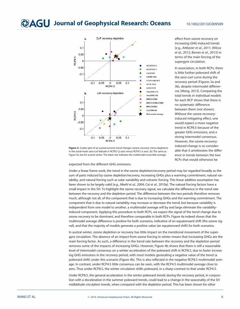
effect from ozone recovery onincreasing GHG-induced trends[e.g., Arblaster et al., 2011; Wilcoxet al., 2012; Barnes et al., 2013] interms of the main forcing of thesupergyre circulation.

In association, in both RCPs, thereis little further poleward shift ofthe zero-curl curve during therecovery period (Figures 3a and3b), despite intermodel differen-ces [Wang, 2013]. Comparing thetotal trends in individual modelsfor each RCP shows that there isno systematic differencebetween them (not shown).Without the ozone-recovery-induced mitigating effect, onewould expect a more negativetrend in RCP8.5 because of thegreater GHG emissions, and astrong intermodel consensus.However, the ozone-recovery-induced change is so consider-able that it ameliorates the differ-ence in trends between the twoRCPs that would otherwise be

expected from the different GHG emissions.

Under a linear frame work, the trend in the ozone depletion/recovery period may be regarded broadly as thesum of parts induced by ozone depletion/recovery, increasing GHGs plus a warming commitment, natural var-iability, and natural forcing such as solar variability and volcanic forcing. This linear additive assumption hasbeen shown to be largely valid [e.g., Meehl et al., 2004; Cai et al., 2010a]. The natural forcing factors have asmall impact in the SH. To highlight the ozone recovery signal, we calculate the difference in the trend ratebetween the recovery and the depletion period. The difference between the two periods therefore removesmuch, although not all, of the component that is due to increasing GHGs and the warming commitment. Thecomponent that is due to natural variability may increase or decrease the trend, but because variability isindependent from one model to another, a multimodel average will by and large eliminate the variability-induced component. Applying this procedure to both RCPs, we expect the signal of the trend change due toozone recovery to be dominant, and therefore comparable in both RCPs. Figure 4a indeed shows that themultimodel average difference is positive for both scenarios, indicative of an equatorward shift (the ozone sig-nal), and that the majority of models generate a positive value (an equatorward shift) for both scenarios.

In austral winter, ozone depletion or recovery has little impact on the meridional movement of the super-gyre circulation. The absence of an impact from ozone forcing in winter means that increasing GHGs are themain forcing factor. As such, a difference in the trend rate between the recovery and the depletion periodremoves some of the impacts of increasing GHGs. However, Figure 4b shows that there is still a reasonablelevel of intermodel consensus on a winter acceleration of the poleward shift in RCP8.5, due to faster increas-ing GHG emissions in the recovery period, with most models generating a negative value of the trend (apoleward shift) under this scenario (Figure 4b). This is also reflected in the negative RCP8.5 multimodel aver-age. In contrast, under RCP4.5 little consensus can be seen, with the RCP4.5 multimodel average close tozero. Thus under RCP8.5, the winter circulation shifts poleward, in a sharp contrast to that under RCP4.5.

Under RCP8.5, the general acceleration in the winter poleward trends during the recovery period, in conjunc-tion with a deceleration in the summer poleward trends, could lead to a change in the seasonality of the SHmidlatitude circulation trends, when compared with the depletion period. This has been shown for other

Figure 4. Scatter plot of (a) austral-summer trend changes (ozone recovery minus depletion)in the zonal-mean zero-curl latitude in RCP8.5 (y axis) versus RCP4.5 (x axis). (b) The same asFigure 4a, but for austral winter. The black star indicates the multimodel ensemble average.

Journal of Geophysical Research: Oceans 10.1002/2013JC009589

WANG ET AL. VC 2014. American Geophysical Union. All Rights Reserved. 6

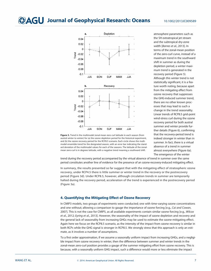
atmosphere parameters such asthe SH extratropical jet streamand the subtropical dry-zonewidth [Barnes et al., 2013]. Interms of the zonal-mean positionof the zero-curl curve, instead of amaximum trend in the southwardshift in summer as during thedepletion period, a winter maxi-mum trend is generated in therecovery period (Figure 5).Although this winter trend is notstatistically significant, it is a fea-ture worth noting, because apartfrom the mitigating effect fromozone recovery that suppressesthe GHG-induced summer trend,there are no other known proc-esses that may lead to such achange in the trend seasonality.Linear trends of RCP8.5 grid-pointwind-stress curl during the ozonerecovery period for both australsummer and winter provide fur-ther details (Figure 6), confirmingthat the recovery-period trend isindeed stronger in winter than insummer. In fact, there is a virtualabsence of a trend in summeralmost everywhere (Figure 6a).The emergence of the winter

trend during the recovery period accompanied by the virtual absence of trend in summer over the sameperiod constitutes another line of evidence for the presence of an ozone-recovery-induced mitigating effect.

In summary, the results presented so far suggest that with the mitigating effect of stratospheric ozonerecovery, under RCP4.5 there is little summer or winter trend in the recovery or the postrecoveryperiod (Figure 3d). Under RCP8.5, however, although circulation trends in summer are temporarilyhalted during the recovery period, acceleration of the trend is experienced in the postrecovery period(Figure 3a).

4. Quantifying the Mitigating Effect of Ozone Recovery

In CMIP3 models, two groups of experiments were conducted; one with time-varying ozone concentrationsand one without; allowing a comparison to gauge the importance of ozone forcing [e.g., Cai and Cowan,2007]. This is not the case for CMIP5, as all available experiments contain similar ozone forcing [e.g., Wilcoxet al., 2012; Eyring et al., 2013]. However, the seasonality of the impact of ozone depletion and recovery andthe general lack of seasonality from increasing GHGs may be used to estimate the ozone-mitigating effect.Again here we focus on the RCP8.5 scenario, as the intensity of the impact from ozone recovery is similar inboth RCPs while the GHG signal is stronger in RCP8.5. We strongly stress that this approach is only an esti-mate, as it involves a number of assumptions.

To a first order approximation, if we assume a seasonally uniform impact from increasing GHGs, and a negligi-ble impact from ozone recovery in winter, then the difference between summer and winter trends in thezonal-mean zero-curl position provides a gauge of the summer mitigating effort from ozone recovery. This isbecause, with a seasonally uniform GHG impact, such a difference would more or less eliminate the impact

Figure 5. Trend in the multimodel zonal-mean zero curl latitude in each season (fromaustral winter to winter) for (a) the ozone depletion period for the historical experiment,and (b) the ozone recovery period for the RCP8.5 scenario. Each circle shows the multi-model ensemble trend for the designated season, with an error bar indicating the stand-ard deviation of the multimodel values for each of the seasons. The latitude of the zonal-mean zero-curl is in degrees latitude, with a negative trend meaning a southward shift.

Journal of Geophysical Research: Oceans 10.1002/2013JC009589

WANG ET AL. VC 2014. American Geophysical Union. All Rights Reserved. 7

from increasing GHGs. As such, the summer-minus-winter difference in each model is calculated. For the mul-timodel average, ozone recovery mitigates the summer poleward shift by 0.87� over the recovery period.

The poleward shift is not additional to, or independent from, the trend in the wind-stress curl field. In fact,the two parameters are closely linked through changing winds. It is the changing winds and the associatedwind-stress curls, which superimpose on the mean curl field, that lead to a change in the zonal-mean lati-tude of the zero-curl curve. Thus, we may use this relationship to estimate the change in the curl field, utiliz-ing the ozone-recovery-induced summer equatorward shift estimated above.

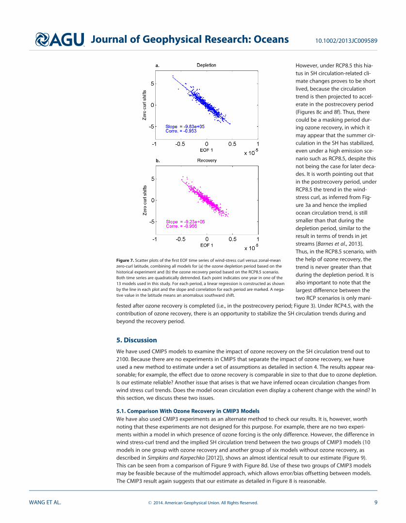
To this end, we apply empirical orthogonal function (EOF) analysis to summer wind-stress curl anomaliesreferenced to the mean over the combined periods (1961–2100). This yields a dominant spatial pattern(EOF1) of the curls (CurlEOF1Pattern (x, y, L), L51:13 representing models). The pattern displays positiveanomalies in the midlatitudes, similar to those shown in Figure 2e. The associated principal componenttime series (CurlEOF1PC(t, L), L51:13 representing models) describes the evolution of the pattern. For eachmodel, a slope, b(L), which represents the sensitivity of the curl pattern to the zero-curl position withouttrends, is obtained by regressing CurlEOF1PC(t, L) onto a quadratically detrended time series of zonal-meanzero-curl position (ZeroCurlPosition(t, L), L51:13 representing models). An aggregation of all models used isdepicted in Figure 7 for the depletion and recovery period. The relationship is almost identical between thetwo periods, indicating its stability from the depletion to the recovery period. For each model, the summertrend of the equatorward shift D(L) by ozone recovery is already estimated as the difference of that insummer minus that in winter, as discussed above.

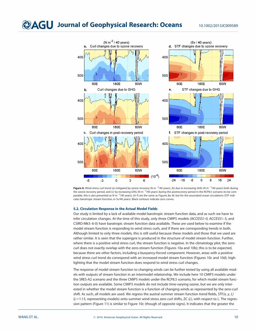
Thus, the wind-stress curl changes due to the mitigating effect of ozone recovery for each model can beestimated by b(L) x D(L) x CurlEOF1Pattern(x, y, L), and the multimodel average (i.e., with respect to L) isplotted in Figure 8a. To take into account the different length of periods, the trend is expressed as thetotal change in a fixed period of 40 years. The total curl trend (filled colors, Figure 6a) is the differencebetween the component induced by GHGs and that mitigated by ozone recovery. In a linear frame work,the GHG-induced component is obtained as the difference between the total and that induced by ozonerecovery, and is shown in Figure 8b. The associated ocean circulation trends are inferred using the IslandRule model [Godfrey, 1989], and displayed in Figures 8d and 8e, for the ozone-recovery-induced andGHG-induced components, respectively. In addition to the impact from ozone recovery being comparableto that from increasing GHGs, which can be inferred from Figure 3a, the impact from ozone recovery isquantified to be significant. Under RCP8.5, an increased trend �6 Sv/40 years in the flow passing throughthe Tasman Sea during the recovery period would have been generated, if not for the offsetting effectfrom ozone recovery. This trend would have further consequences in terms of regional sea level rise andchanges in marine biodiversity boundaries, among other things, but is modeled to be mitigated by strato-spheric ozone recovery.

Figure 6. Climatological wind-stress curl (contours) and wind-stress curl trend (colors) from the multimodel ensemble average over therecovery period in (a) austral summer and (b) austral winter for RCP8.5. (c and d) Zonal average of wind-stress curl trends in Figures 6a and6b, respectively. Black contours indicate the zero-curl curves, red (blue) contours indicate positive (negative) curls. Unit: N m23/yr.

Journal of Geophysical Research: Oceans 10.1002/2013JC009589

WANG ET AL. VC 2014. American Geophysical Union. All Rights Reserved. 8

However, under RCP8.5 this hia-tus in SH circulation-related cli-mate changes proves to be shortlived, because the circulationtrend is then projected to accel-erate in the postrecovery period(Figures 8c and 8f). Thus, therecould be a masking period dur-ing ozone recovery, in which itmay appear that the summer cir-culation in the SH has stabilized,even under a high emission sce-nario such as RCP8.5, despite thisnot being the case for later deca-des. It is worth pointing out thatin the postrecovery period, underRCP8.5 the trend in the wind-stress curl, as inferred from Fig-ure 3a and hence the impliedocean circulation trend, is stillsmaller than that during thedepletion period, similar to theresult in terms of trends in jetstreams [Barnes et al., 2013].Thus, in the RCP8.5 scenario, withthe help of ozone recovery, thetrend is never greater than thatduring the depletion period. It isalso important to note that thelargest difference between thetwo RCP scenarios is only mani-

fested after ozone recovery is completed (i.e., in the postrecovery period; Figure 3). Under RCP4.5, with thecontribution of ozone recovery, there is an opportunity to stabilize the SH circulation trends during andbeyond the recovery period.

5. Discussion

We have used CMIP5 models to examine the impact of ozone recovery on the SH circulation trend out to2100. Because there are no experiments in CMIP5 that separate the impact of ozone recovery, we haveused a new method to estimate under a set of assumptions as detailed in section 4. The results appear rea-sonable; for example, the effect due to ozone recovery is comparable in size to that due to ozone depletion.Is our estimate reliable? Another issue that arises is that we have inferred ocean circulation changes fromwind stress curl trends. Does the model ocean circulation even display a coherent change with the wind? Inthis section, we discuss these two issues.

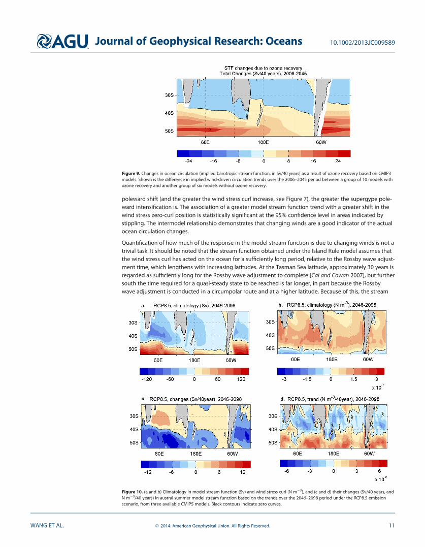
5.1. Comparison With Ozone Recovery in CMIP3 ModelsWe have also used CMIP3 experiments as an alternate method to check our results. It is, however, worthnoting that these experiments are not designed for this purpose. For example, there are no two experi-ments within a model in which presence of ozone forcing is the only difference. However, the difference inwind stress-curl trend and the implied SH circulation trend between the two groups of CMIP3 models (10models in one group with ozone recovery and another group of six models without ozone recovery, asdescribed in Simpkins and Karpechko [2012]), shows an almost identical result to our estimate (Figure 9).This can be seen from a comparison of Figure 9 with Figure 8d. Use of these two groups of CMIP3 modelsmay be feasible because of the multimodel approach, which allows error/bias offsetting between models.The CMIP3 result again suggests that our estimate as detailed in Figure 8 is reasonable.

Figure 7. Scatter plots of the first EOF time series of wind-stress curl versus zonal-meanzero-curl latitude, combining all models for (a) the ozone depletion period based on thehistorical experiment and (b) the ozone recovery period based on the RCP8.5 scenario.Both time series are quadratically detrended. Each point indicates one year in one of the13 models used in this study. For each period, a linear regression is constructed as shownby the line in each plot and the slope and correlation for each period are marked. A nega-tive value in the latitude means an anomalous southward shift.

Journal of Geophysical Research: Oceans 10.1002/2013JC009589

WANG ET AL. VC 2014. American Geophysical Union. All Rights Reserved. 9

5.2. Circulation Response in the Actual Model FieldsOur study is limited by a lack of available model barotropic stream function data, and as such we have toinfer circulation changes. At the time of this study, only three CMIP5 models (ACCESS1-0, ACCESS1–3, andCSIRO-Mk3–6-0) have baratropic stream function data available. These are used below to examine if themodel stream function is responding to wind stress curls, and if there are corresponding trends in both.Although limited to only three models, this is still useful because these models and those that we used arerather similar. It is seen that the supergyre is produced in the structure of model stream function. Further,where there is a positive wind stress curl, the stream function is negative. In the climatology plot, the zero-curl does not exactly overlap with the zero-stream function (Figures 10a and 10b); this is to be expected,because there are other factors, including a buoyancy-forced component. However, areas with a positivewind stress curl trend do correspond with an increased model stream function (Figures 10c and 10d), high-lighting that the model stream function does respond to wind stress curl changes.

The response of model stream function to changing winds can be further tested by using all available mod-els with outputs of stream function in an intermodel relationship. We include here 10 CMIP3 models underthe SRES-A2 scenario and the three CMIP5 models under the RCP8.5 scenario, for which model stream func-tion outputs are available. Some CMIP3 models do not include time-varying ozone, but we are only inter-ested in whether the model stream function is a function of changing winds as represented by the zero-curlshift. As such, all models are used. We regress the austral summer stream function trend fields, STF(x, y, L)(L51:13, representing models) onto summer wind stress zero curl shifts, ZC (L), with respect to L. The regres-sion pattern (Figure 11) is similar to Figure 10c (though of opposite signs). It indicates that the greater the

Figure 8. Wind-stress curl trend (a) mitigated by ozone recovery (N m23/40 years), (b) due to increasing GHG (N m23/40 years) both duringthe ozone recovery period, and (c) by increasing GHG (N m23/40 years) during the postrecovery period in the RCP8.5 scenario (to be com-parable, this is also presented as N m23/40 years); (d–f) are the same as Figures 8a–8c but for the associated ocean circulations (STF indi-cates barotropic stream function, in Sv/40 years). Black contours indicate zero curves.

Journal of Geophysical Research: Oceans 10.1002/2013JC009589

WANG ET AL. VC 2014. American Geophysical Union. All Rights Reserved. 10

poleward shift (and the greater the wind stress curl increase, see Figure 7), the greater the supergype pole-ward intensification is. The association of a greater model stream function trend with a greater shift in thewind stress zero-curl position is statistically significant at the 95% confidence level in areas indicated bystippling. The intermodel relationship demonstrates that changing winds are a good indicator of the actualocean circulation changes.

Quantification of how much of the response in the model stream function is due to changing winds is not atrivial task. It should be noted that the stream function obtained under the Island Rule model assumes thatthe wind stress curl has acted on the ocean for a sufficiently long period, relative to the Rossby wave adjust-ment time, which lengthens with increasing latitudes. At the Tasman Sea latitude, approximately 30 years isregarded as sufficiently long for the Rossby wave adjustment to complete [Cai and Cowan 2007], but furthersouth the time required for a quasi-steady state to be reached is far longer, in part because the Rossbywave adjustment is conducted in a circumpolar route and at a higher latitude. Because of this, the stream

Figure 9. Changes in ocean circulation (implied barotropic stream function, in Sv/40 years) as a result of ozone recovery based on CMIP3models. Shown is the difference in implied wind-driven circulation trends over the 2006–2045 period between a group of 10 models withozone recovery and another group of six models without ozone recovery.

Figure 10. (a and b) Climatology in model stream function (Sv) and wind stress curl (N m23), and (c and d) their changes (Sv/40 years, andN m23/40 years) in austral summer model stream function based on the trends over the 2046–2098 period under the RCP8.5 emissionscenario, from three available CMIP5 models. Black contours indicate zero curves.

Journal of Geophysical Research: Oceans 10.1002/2013JC009589

WANG ET AL. VC 2014. American Geophysical Union. All Rights Reserved. 11

function calculated using the Island Rule model is generally greater than the model stream function, exceptfor in regions where a quasi-steady state can be assumed, such as the Tasman Sea. In such regions, themodel stream function trend is about 6 Sv per 40 years (Figure 10c), comparable to that obtained from theIsland Rule calculation.

6. Conclusions

The Antarctic stratospheric ozone depletion that occurred in the latter part of the 20th century has domi-nated the observed trends in SH circulation during austral summer over the past decades. However, as aresult of the successful implementation of the Montr�eal protocol [e.g., Barnes et al., 2013], Antarctic ozone isprojected to recover by the middle of the 21st century. The recovery provides a mechanism for offsettingthe impact of increasing GHG emissions. We examine CMIP5 model experiments with the historical, RCP4.5and RCP8.5 emission scenarios. We show that during the recovery period (2006–2045), the summer trend ofthe poleward shift of the supergyre circulation is substantially offset. In fact, the mitigating effect of ozonerecovery is so dominant that there is little difference in the summer trends between the two RCP scenarios,despite their difference in GHG emissions. Furthermore, the trend of the poleward shift of the supergyre cir-culation in winter, a season in which ozone recovery has little impact, is greater (more poleward) than thatin summer under RCP8.5, opposite to the seasonality of trends during the depletion period. Under RCP4.5,with the contribution from ozone recovery, the summer poleward shift of the supergyre is projected to sta-bilize into the postrecovery decades (2046–2100), whereas under RCP8.5, the summer poleward shift in thepostrecovery period accelerates, presenting two vastly different ocean circulation futures dependent on theemission pathway society decides to take.

ReferencesArblaster, J. M., G. A. Meehl, and D. J. Karoly (2011), Future climate change in the Southern Hemisphere: Competing effects of ozone and

greenhouse gases, Geophys. Res. Lett., 38, L02701, doi:10.1029/2010GL045384.Barnes, E., N. Barnes, and L. Polvani (2013), Delayed Southern Hemisphere climate change induced by stratospheric ozone recovery, as pro-

jected by the CMIP5 models, J. Clim., 27, 852–867, doi:10.1175/JCLI-D-13-00246.1.De Boer, A. M., R. M. Graham, M. D. Thomas, and K. E. Kohfeld (2013), The control of the Southern Hemisphere Westerlies on the position of

the Subtropical Front, J. Geophys. Res. Oceans, 118, 5669–5675, doi:10.1002/jgrc.20407.Cai, W. (2006), Antarctic ozone depletion causes an intensification of the Southern Ocean super-gyre circulation, Geophys. Res. Lett., 33,

L03712, doi:10.1029/2005GL024911.Cai, W., and T. Cowan (2007), Trends in Southern Hemisphere circulation in IPCC AR4 models over 1950–1999: Ozone-depletion vs. green-

house forcing, J. Clim., 20(4), 681–693.Cai, W., P. H. Whetton, and D. J. Karoly (2003), The response of the Antarctic oscillation to increasing and stabilized atmospheric CO2,

J. Clim., 16, 1525–1538, doi:10.1175/1520-0442-16.10.1525.Cai, W., T. Cowan, J. M. Arblaster, and S. Wijffels (2010a), On potential causes for an underestimated global ocean heat content trend in

CMIP3 models, Geophys. Res. Lett., 37, L17709, doi:10.1029/2010GL044399.

Figure 11. Intermodel regression coefficients between model stream function trends and zero curl shifts (Sv/(degree latitude)), calculated byregressing the total barotropic stream function trend field STF(x,y,L) (L 5 1:13, representing models) onto the total zero curl shifts, ZC(L), from2046 to 2098 in austral winter under RCP8.5 and A2 emission scenarios. The regression is carried out with respect to L.

AcknowledgmentsThis work was carried out whileGuojian Wang was a PhD student ofthe Ocean University of China,supported by a scholarship from theChina Scholarship Council, whichenabled his visit to CSIRO Marine andAtmospheric Research. Wenju Cai andAriaan Purich are supported by theAustralian Climate Change ScienceProgramme.

Journal of Geophysical Research: Oceans 10.1002/2013JC009589

WANG ET AL. VC 2014. American Geophysical Union. All Rights Reserved. 12

Cai, W., T. Cowan, S. Godfrey, and S. Wijffels (2010b), Simulations of processes associated with the fast warming rate of the southern midla-titude ocean, J. Clim., 23, 197–206, doi:10.1175/2009JCLI3081.1.

Carril, A. F., C. G. Men�endez, and A. Navarra (2005), Climate response associated with the Southern Annular Mode in the surroundings ofAntarctic Peninsula: A multimodel ensemble analysis, Geophys. Res. Lett., 32, L16713, doi:10.1029/2005GL023581.

Eyring, V., et al. (2013), Long-term ozone changes and associated climate impacts in CMIP5 simulations, J. Geophys. Res. Atmos., 118, 5029–5060, doi:10.1002/jgrd.50316.

Fogt, R. L., J. Perlwitz, A. J. Monaghan, D. H. Bromwich, J. M. Jones, and G. J. Marshall (2009), Historical SAM variability. Part II: Twentieth-century variability and trends from reconstructions, observations, and the IPCC AR4 models, J. Clim., 22, 5346–5365.

Gille, S. T. (2008), Decadal-scale temperature trends in the Southern Hemisphere ocean, J. Clim., 21, 4749–4765.Gillett, N. P., and D. W. J. Thompson (2003), Simulation of recent Southern Hemisphere climate change, Science, 302, 273–275.Godfrey, J. S. A. (1989), Sverdrup model of the depth-integrated flow for the world ocean allowing for island circulations, Geophys. Astro-

phys. Fluid Dyn., 45, 89–112.Kalnay, E., et al. (1996), The NCEP/NCAR 40-year reanalysis project, Bull. Am. Meteorol. Soc., 3, 437–471.Kang, S. M., L. M. Polvani, J. C. Fyfe and M. Sigmond (2011), Impact of polar ozone depletion on subtropical precipitation, Science,

332(6032), 951–954, doi:10.1126/science.1202131.Karoly, D. J. (1990), The role of transient eddies in low-frequency zonal variations of the Southern Hemisphere circulation, Tellus, Ser. A, 42, 41–50.Kidson, J. W. (1988), Interannual variations in the Southern Hemisphere circulation, J. Clim., 1, 1177–1198.Lee, S., and S. B. Feldstein (2013), Detecting ozone- and greenhouse gas-driven wind trends with observational data, Science, 339(6119),

563–567, doi:10.1126/science.1225154.Marshall, G. J. (2003), Trends in the southern annular mode from observations and reanalyses, J. Clim., 16, 4134–4143.Marshall, G. J., P. A. Scott, J. Turner, W. M. Connolley, J. C. King, and T. A. Lachlan-Cope (2004), Causes of exceptional atmospheric circulation

changes in the Southern Hemisphere, Geophys. Res. Lett., 31, L14205, doi:10.1029/2004GL019952.Meehl, G. A., W. M. Washington, C. M. Ammann, J. M. Arblaster, T. M. L. Wigley, and C. Tebaldi (2004), Combinations of natural and anthro-

pogenic forcings in twentieth-century climate, J. Clim, 17, 3721–3727.Meinshausen, M., et al. (2011), The RCP greenhouse gas concentrations and their extensions from 1765 to 2300, Clim. Change, 109(1–2),

213–241, doi:10.1007/s10584-011-0156-z.Miller, R., G. Schmidt, and D. Shindell (2006), Forced annular variations in the 20th century intergovernmental panel on climate change

fourth assessment report models, J. Geophys. Res., 111, D18101, doi:10.1029/2005JD006323.Polvani, L., D. Waugh, G. Correa, and S. Son (2011), Stratospheric ozone depletion: The main driver of twentieth-century atmospheric circu-

lation changes in the Southern Hemisphere, J. Clim., 24, 795–812, doi:10.1175/2010JCLI3772.1.Purich, A., and S. W. Son (2012), Impact of Antarctic ozone depletion and recovery on Southern Hemisphere precipitation, evaporation,

and extreme changes, J. Clim., 25, 3145–3154, doi:10.1175/JCLI-D-11-00383.1.Purich, A., T. Cowan, S.-K. Min, and W. Cai (2013), Autumn precipitation trends over Southern Hemisphere Midlatitudes as simulated by

CMIP5 models, J. Clim., 26, 8341–8356, doi:10.1175/JCLI-D-13-00007.1.Randel, W. J., and F. Wu (1999), Cooling of the Arctic and Antarctic polar stratospheres due to ozone depletion, J. Clim., 12, 1467–1469.Ridgway, K. R., and J. R. Dunn (2007), Observational evidence for a Southern Hemisphere oceanic supergyre, Geophys. Res. Lett., 34, L13612,

doi:10.1029/2007GL030392.Roemmich, D., J. Gilson, R. Davis, P. Sutton, S. Wijffels, and S. Riser (2007), Decadal spinup of the South Pacific subtropical gyre, J. Phys. Oce-

anogr., 37, 162–173, doi:10.1175/JPO3004.1.Roscoe, H., and J. Haigh (2007), Influences of ozone depletion, the solar cycle and the QBO on the Southern Annular Mode, Q. J. R. Meteorol.

Soc., 1864, 1855–1864, doi:10.539 1002/qj.Russell, J. L., K. W. Dixon, A. Gnanadesikan, R. J. Stouffer, J. R. Toggweiler (2006), The Southern Hemisphere westerlies in a warming world:

Propping open the door to the deep ocean, J. Clim., 19, 6382–6390, doi:10.1175/JCLI3984.1.Scheff, J., and D. Frierson (2012b), Twenty-first-century multimodel subtropical precipitation declines are mostly midlatitude shifts, J. Clim.,

25, 4330–4347, doi:10.1175/JCLI-D-11-00393.1.Simpkins, G. R., and A. Y. Karpechko (2012), Sensitivity of the southern annular mode to greenhouse gas emission scenarios. Clim. Dyn, 38, 563–572.Solomon, S., R. W. Portmann, T. Sasaki, D. J. Hofman, and D. W. J. Thompson (2006), Four decades of ozonesonde measurements over Ant-

arctica, J. Geophys. Res., 110, D21311, doi:10.1029/2005JD005917.Son, S. W., L. M. Polvani, D. W. Waugh, H. Akiyoshi, R. Garcia, D. Kinnison, S. Pawson, E. Rozanov, T. G. Shepherd, K. Shibata (2008), The

impact of stratospheric ozone recovery on the Southern Hemisphere westerly jet, Science, 320(5882), 1486–1489, doi:10.1126/science.1155939.

Son, S. W., N. F. Tandon, L. M. Polvani, and D. W. Waugh (2009), Ozone hole and Southern Hemisphere climate change, Geophys. Res. Lett.,36, L15705, doi:10.1029/2009GL038671.

Taylor, K. E., R. J. Stouffer, and G. A. Meehl (2012), An overview of CMIP5 and the experiment design, Bull. Am. Meteorol. Soc., 93, 485–498,doi:10.1175/BAMS-D-11-00094.1.

Thompson, D. W. J., and S. Solomon (2002), Interpretation of recent Southern Hemisphere climate change, Science, 296, 895–899, doi:10.1126/science.1069270.

Thompson, D. W. J., S. Solomon, P. J. Kushner, M. H. England, K. M. Grise, and D. J. Karoly (2011), Signatures of the Antarctic ozone hole inSouthern Hemisphere surface climate change, Nat. Geosci., 4, 741–749, doi:10.1038/ngeo1296.

Wang, G., and W. Cai (2013), Climate-change impact on the 20th-century relationship between the Southern Annular Mode and globalmean temperature, Sci. Rep., 3, 2039, doi:10.1038/srep02039.

Wang, Z. (2013), On the response of Southern Hemisphere subpolar gyres to climate change in coupled climate models, J. Geophys. Res.Oceans, 118, 1070–1086, doi:10.1002/jgrc.20111.

Waugh, D. W., W. J. Randel, S. Pawson, P. A. Newman, and E. R. Nash (1999), Persistence of the lower stratospheric polar vortices, J. Geophys.Res., 104, 27,191–27,202.

Wilcox, L. J., A. J. Charlton-Perez, and L. J. Gray (2012), Trends in Austral jet position in ensembles of high- and low-top CMIP5 models,J. Geophys. Res., 117, D13115, doi:10.1029/2012JD017597.

Wu, L., et al. (2012), Enhanced warming over the global subtropical western boundary current, Nat. Clim. Change, 2, 161–166, doi:10.10.1038/nclimate1353.

Zhou, S. T., M. E. Gelman, A. J. Miller, and J. P. McCormack (2000), An inter-hemisphere comparison of the persistent stratospheric polar vor-tex, Geophys. Res. Lett., 27, 1123–1126.

Journal of Geophysical Research: Oceans 10.1002/2013JC009589

WANG ET AL. VC 2014. American Geophysical Union. All Rights Reserved. 13