Modelling Northern Hemisphere ice sheets distribution during MIS5 and MIS7 glacial inceptions

CPD8, 6221–6267, 2012

Investigating MIS5and MIS7 glacial

inceptions

F. Colleoni et al.

Title Page

Abstract Introduction

Conclusions References

Tables Figures

J I

J I

Back Close

Full Screen / Esc

Printer-friendly Version

Interactive Discussion

Discussion

Paper

|D

iscussionP

aper|

Discussion

Paper

|D

iscussionP

aper|

Clim. Past Discuss., 8, 6221–6267, 2012www.clim-past-discuss.net/8/6221/2012/doi:10.5194/cpd-8-6221-2012© Author(s) 2012. CC Attribution 3.0 License.

Climateof the Past

Discussions

This discussion paper is/has been under review for the journal Climate of the Past (CP).Please refer to the corresponding final paper in CP if available.

Modelling Northern Hemisphere icesheets distribution during MIS5 andMIS7 glacial inceptions

F. Colleoni1, S. Masina1,2, A. Cherchi1,2, A. Navarra1,2, C. Ritz3, V. Peyaud3, andB. Otto-Bliesner4

1Centro Euro-Mediterraneo per i Cambiamenti Climatici, Bologna, Italy2Istituto Nazionale di Geofisica e di Vulcanologia, Bologna, Italy3CNRS/Universite Joseph Fourier, Grenoble 1, LGGE, St Martin d’Heres cedex, France4Climate and Global Dynamics Division, National Center for Atmospheric Research, Boulder,CO, USA

Received: 14 November 2012 – Accepted: 5 December 2012 – Published: 18 December 2012

Correspondence to: F. Colleoni ([email protected])

Published by Copernicus Publications on behalf of the European Geosciences Union.

6221

http://www.clim-past-discuss.net

http://www.clim-past-discuss.net/8/6221/2012/cpd-8-6221-2012-print.pdf

http://www.clim-past-discuss.net/8/6221/2012/cpd-8-6221-2012-discussion.html

http://creativecommons.org/licenses/by/3.0/

CPD8, 6221–6267, 2012


inceptions

F. Colleoni et al.

Title Page



Tables Figures

J I

J I

Back Close

Full Screen / Esc



Discussion

Paper

|D

iscussionP

aper|

Discussion

Paper

|D

iscussionP

aper|

Abstract

The present manuscript compares the last two glacial inceptions, Marine Isotope Stage5 (MIS5, 125–115 kyr BP) and MIS7 (236–229 kyr BP) with the aim to detect the rela-tive impact of external forcing (orbitals and GHG) and ice-albedo feedbacks on theice sheets growth and distribution in the Northern Hemisphere high latitudes. In or-5

der to investigate the differences between those two states, we combine atmosphere-ocean coupled model experiments and off-line ice-sheet-model simulations. In partic-ular, we use a low resolution coupled Atmosphere-Ocean-Sea-ice general circulationmodel to simulate the mean climate of the four time periods associated with the in-ception states of MIS5 and MIS7 (i.e. 236, 229, 125 and 115 kyr BP). The four mean10

states are then use to force a 3-D thermodynamical ice sheet model by means oftwo types of ice sheet experiments, i.e., steady-state and transient experiments. Ourresults show that steady-state ice experiments underestimate the ice volume at both229 kyr BP and 115 kyr BP. On the other hand, the simulated pre-inception ice distribu-tions at 236 kyr BP and 125 kyr BP are in good agreement with observations indicating15

that during these periods feedbacks associated with external forcing dominate overother processes. However, if proper ice-elevation and albedo feedbacks are not takeninto consideration, the evolution towards glacial inception in terms of ice volume andextent is hardly simulated. The experimental setup chosen allows us to conclude that,depending on the mean background climate state, the effect of model biases on cli-20

mate are more important during a cold inception, such as MIS7, than during a warminception, such as MIS5. The last results suggest to be cautious when tuning and cal-ibrating Earth System Models on a specific time period, mainly for the purpose of icesheet-climate coupling.

6222





CPD8, 6221–6267, 2012


inceptions

F. Colleoni et al.

Title Page



Tables Figures

J I

J I

Back Close

Full Screen / Esc



Discussion

Paper

|D

iscussionP

aper|

Discussion

Paper

|D

iscussionP

aper|

1 Introduction

Glacial inceptions represent a transition from a warm to a cold mean climate state(Calov et al., 2005b). Indeed, considering the sea level record during these warm-to-cold transitions, Northern Hemisphere ice sheets were only little developed overNorth America and Eurasia compared to glacial maxima (Fig. 1d). Concerns about5

the capability of climate models to properly simulate future climates have emergedfrom the large uncertainties and lack of flexibility of the same models to simulate pastclimate transitions from warm to cold conditions (Calov et al., 2005b). Therefore, glacialinceptions are an interesting phenomenon with which to test the capability of modelsto simulate climates slightly warmer or slightly colder than present-day climates.10

It is now accepted that Northern Hemisphere ice sheets started to develop only ifboth insolation and greenhouse gases (GHG) dropped significantly (e.g. Berger, 1978;Bonelli et al., 2009). But are all glacial inceptions similar in term of initial continentalice volume? While the maximum sea-level fall was similar between the last two glacialcycles, the maximum sea-level rise during the last two interglacials (≈135 kyr BP and15

≈245 kyr BP) varies with estimates above or below present-day sea level (Fig. 1d, Ra-bineau et al., 2006; Caputo, 2007). Indeed, for the last interglacial (≈135 kyr BP), prox-ies indicate a sea-level rise between 4 to 10 m above mean sea-level (a.m.s.l., Stir-ling et al., 1995; Kopp et al., 2009; McCulloch and Esat, 2000) implying that part ofpresent-day Antarctica and Greenland ice sheets melted out. In contrast, Dutton et al.20

(2009) suggest that during the penultimate interglacial, ≈245 kyr BP, sea-level neverrose above present-day mean sea-level. All together, these observations suggest thatthe amount of continental ice melting differed from one interglacial to another and thatthe inception of each glacial cycle had different initial conditions at the surface, es-pecially in terms of ice distribution and ice volume stored on the continents. Because25

of those sea-level characteristics, in this work we focus on the last two glacial incep-tions, Marine Isotope Stage 5 (MIS5, ≈125–116 kyr BP) and MIS7 (≈236–229 kyr BP),respectively.

6223





CPD8, 6221–6267, 2012


inceptions

F. Colleoni et al.

Title Page



Tables Figures

J I

J I

Back Close

Full Screen / Esc



Discussion

Paper

|D

iscussionP

aper|

Discussion

Paper

|D

iscussionP

aper|

Numerous studies have tackled the glacial inception issue using Atmospheric Gen-eral Circulation Models (AGCM, e.g. Rind et al., 1989; Dong and Valdes, 1995; Vet-toretti and Peltier, 2003), coupled Atmosphere-Ocean GCMs (AOGCM, e.g. Khodriet al., 2001; Yoshimori et al., 2002), Earth system Models of Intermediate Complexity(EMIC, e.g. Meissner et al., 2003), and three-dimensional ice sheets models coupled5

to EMIC (e.g. Calov and Marsiat, 1998; Bonelli et al., 2009). The majority of paleocli-mate modelling studies have focused on the last glacial inception (≈115 kyr BP) andhave simulated a sea-level drop by estimating the amount of perennial snow accumu-lated over the Northern Hemisphere high latitudes using steady-state experiments (e.g.Vettoretti and Peltier, 2003; Jochum et al., 2012) or transient experiments (e.g. Wang10

and Mysak, 2002). These models have shown that they can broadly simulate perennialsnow and ice sheets growth in the Northern Hemisphere high latitudes where geolog-ical evidence are indicative of glacial inception areas. Other studies have performedidealized experiments to determine the thresholds of various regional feedbacks inthe climate system that could have triggered a glacial inception in the Northern Hemi-15

sphere high latitudes (e.g. Calov et al., 2005a,b). Some of the modeling studies haveshown the importance of vegetation and dust in amplifying or inhibiting the growth ofthe ice sheets during the last two glacial cycles (e.g. de Noblet et al., 1996; Vettorettiand Peltier, 2004; Kageyama et al., 2004; Calov et al., 2005a; Krinner et al., 2006;Colleoni et al., 2009a,b). Kubatzki et al. (2006), using a fully coupled climate-ice-sheet20

EMIC, showed that during the last glacial inception (≈113 kyr BP in their study) thegrowth of the Laurentide ice sheet could have been delayed by modulating the state ofocean and vegetation. Furthermore, another recent modeling study focusing on the lastglacial inception (≈115 kyr BP) suggests that the growth of the Eurasian ice sheet atthis time was delayed by a persistent high oceanic heat transport towards the Northern25

Hemisphere high-latitude regions (Born et al., 2010).Those feedbacks might have not been of similar importance for all the glacial in-

ceptions and therefore it is interesting to determine what were the characteristics ofthe global climate preceding the inceptions. Recently, Masson-Delmotte et al. (2010)

6224





CPD8, 6221–6267, 2012


inceptions

F. Colleoni et al.

Title Page



Tables Figures

J I

J I

Back Close

Full Screen / Esc



Discussion

Paper

|D

iscussionP

aper|

Discussion

Paper

|D

iscussionP

aper|

discussed the glacial and interglacial intensities inferred from various climate proxiesretrieved from EPICA Dome C, East Antarctica, ice core records. In their work, the lastinterglacial (≈130 kyr BP) appears to be the warmest of the last 800 kyr and was pre-ceded by one of the mildest glacial periods on record, characterized by a moderate sealevel drop similar to that occurred at the LGM. In contrast, the penultimate interglacial5

(≈245 kyr BP) was cool and was preceded by one of the coldest glacial periods onrecord, characterized by a large drop in sea level. In addition, during the last two in-terglacials, the concentration of atmospheric CO2 retrieved from East Antarctica (Luthiet al., 2008) peaked to a rather similar value, but dropped by a larger amount during thepenultimate glacial inception (Fig. 1f). Indeed, after ≈242 kyr BP CO2 dropped well be-10

low 260 ppm, while after 125 kyr BP, CO2 remained above 260 ppm until ≈110 kyr BP.Similarities with GHGs trends are also observed in East Antarctica mean annual tem-perature anomaly record (Jouzel et al., 2007). In addition the atmospheric CH4 concen-tration shows trends similar to CO2 after both terminations (Fig. 1e, Loulergue et al.,2008). This supports one of the main conclusions of Masson-Delmotte et al. (2010):15

“cooler” interglacials are preceded by colder glaciations, during which the ice-albedofeedback is particularly large and atmospheric GHGs concentrations are particularlylow.

To test the relative importance of orbitals, GHGs and ice-albedo feedbacks on glacialinception processes, we choose to compare the last two glacial inception periods, MIS520

(≈125–116 kyr BP) and MIS7 (≈236–229 kyr BP) respectively. More specifically we in-vestigate the impact of orbital parameters and GHGs on the growth of ice sheets in theNorthern Hemisphere high latitudes. In that context, the last two inceptions are partic-ularly suitable to test the efficiency of the models used here since the MIS5 inceptionis globally warmer than MIS7. We use an Earth System Model (in its fully AOGCM25

coupled version) to simulate the climate of those inceptions, and we further use thatclimate to force a dynamical ice sheet model. In the following sections, the focus ison the ice sheet simulations and the description of the simulated climate dynamics is

6225





CPD8, 6221–6267, 2012


inceptions

F. Colleoni et al.

Title Page



Tables Figures

J I

J I

Back Close

Full Screen / Esc



Discussion

Paper

|D

iscussionP

aper|

Discussion

Paper

|D

iscussionP

aper|

here restricted to the variables needed by the ice sheet model. Finally the discussionhighlights the main weaknesses of the results obtained in this work.

2 Methods

Since the climate model that we use in this work does not have any dynamical icesheet component coupled to atmosphere and ocean, we force offline a 3-D thermo-5

dynamical ice sheet model with our climate simulations. Calov et al. (2009) showedthat asynchronous simulations between climate models and ice sheet models in thecontext of glacial inception are as satisfying as coupled climate-ice sheet simulations.The only difficulty with this method is to account for the evolution in time of the mainfeedbacks that trigger glacial inception. Therefore, to compensate for this problem, we10

modulate the climate forcing in our ice sheet experiments by means of a temperatureindex retrieved from Greenland ice cores. This method has been already used in sev-eral studies focusing on particular slices of the last cycle and has provided realisticresults of the ice sheet evolution (Peyaud et al., 2007; Charbit et al., 2002).

2.1 Community Earth System Model15

To simulate past climates, we use the CESM 1.0, which consists of a fully coupledatmosphere-ocean-sea-ice-land model (Gent et al., 2011). The atmospheric compo-nent CAM has 26 vertical levels and an horizontal resolution grid of 96×48 (T31)shared with the land component (CLM). The ocean component (POP, displaced polelocated over Greenland) has 60 vertical levels and a nominal 3◦ horizontal resolution in20

common with the sea-ice component (CICE). CESM 1.0 provides the possibility of com-puting dynamical vegetation and dynamical aeolian dust distribution, but we turned offthose options and prescribed the pre-industrial vegetation cover and dust distributionover continents in all our experiments since in this work we focus only on the impact ofexternal forcing on the Earth’s climate.25

6226





CPD8, 6221–6267, 2012


inceptions

F. Colleoni et al.

Title Page



Tables Figures

J I

J I

Back Close

Full Screen / Esc



Discussion

Paper

|D

iscussionP

aper|

Discussion

Paper

|D

iscussionP

aper|

CESM experiments setup

The two glacial inceptions under investigation have been selected using the valuesof the proxy records displayed in Fig. 1. The four snapshots referring to the inceptionperiods are identified by the vertical blue boxes. For the last glacial cycle, the timingof inception is commonly defined in literature between 116–113 kyr BP. In this study,5

we set up the inception simulation with 115 kyr BP orbital and GHG values. Deter-mining the timing of the penultimate inception was harder since, as observed on thesea-level records (Fig. 1d), the penultimate glacial cycle does not exhibit a regular de-creasing trend in sea level as for the last glacial cycle. This period is characterized bythree sea-level high-stands (even if below present-day sea level), the first one occur-10

ring right after Termination III towards ≈231 kyr BP, the second one occurring towards≈206 kyr BP and the last one occurring toward ≈189 kyr BP (Dutton et al., 2009). Con-sidering the sea level evolution, the penultimate inception occurred after 189 kyr BP.On the other hand, considering GHGs and Antarctica temperature anomaly, the largestpeaks occurred right after Termination III, setting the beginning of a new cycle towards15

240 kyr BP (Fig. 1e and f). Taking the peak GHGs as reference state for the beginningof the new cycle, we selected the penultimate inception period using the epoch of thenearest orbital state presenting characteristics similar with the inception at 115 kyr BP.The simulation was consequently set up with 229 kyr BP orbitals and GHGs values.As stated in the introduction, the climate evolution before those two glacial inceptions20

was different (Masson-Delmotte et al., 2010). To account for this difference in our icesheets simulations we set up two additional simulations with settings that were definedat the time of the highest sea level preceding each glacial inceptions (Fig. 1d): one at125 kyr BP and one at 236 kyr BP.

In summary, five experiments, different in orbital parameters and atmospheric green-25

house gas concentrations, were carried out to explore the discrepancies between MIS5and MIS7 glacial inceptions: a present-day run (CTR0k) accounting for present-dayGHGs values; a control run set to pre-industrial initial conditions (CTR1850); two MIS5

6227





CPD8, 6221–6267, 2012


inceptions

F. Colleoni et al.

Title Page



Tables Figures

J I

J I

Back Close

Full Screen / Esc



Discussion

Paper

|D

iscussionP

aper|

Discussion

Paper

|D

iscussionP

aper|

experiments set at 125 kyr BP (K125) and 115 kyr BP (K115) and two MIS7 experimentsset at 236 kyr BP (K236) and 229 kyr BP (K229) (see Table 1). The two inceptions ex-periments, K115 and K229, were branched from K125 and K236 respectively after400 yr of simulation and were then continued over 700 yr. However, to compare thesame model years with the branch experiments, CTR1850, K125 and K236 were also5

continued to 700 model years. A slight drift still persists in the experiments due to theabyssal circulation (not shown). However, we assume that this drift is small enough tonot affect our main conclusions.

2.2 Grenoble Ice Shelf and Land Ice model

Since the CESM 1.0 does not include a fully-coupled ice sheet model, we force the10

stand-alone GRISLI ice sheet model (Ritz et al., 2001) using the mean climate statescomputed from our experiments (Table 1). GRISLI is a 3-D-thermodynamical ice sheet– ice stream – ice shelf model, able to simulate both grounded and floating ice. Thegrounded part uses the shallow ice approximation and the ice shelves are thermo-mecanically coupled to the land-ice part. Ice streams are triggered when the sediment15

layer is saturated by water. For more details about the physics, the reader may refer toRommelaere and Ritz (1996) and Ritz et al. (2001).

The experiments have been designed on a regular rectangular grid of 40 km reso-lution from ≈47◦ N to the North Pole. Since we focus on glacial inceptions and we donot have any informations about dimensions of the Greenland ice sheet for the periods20

we are modeling, we start our experiments with the present-day Greenland ice sheettopography adapted from ETOPO2 dataset (NOAA, http://www.ngdc.noaa.gov/mgg/global/etopo2.html). However, the spin-up of the Greenland ice sheet to the time pe-riods considered is simulated through our steady-state experiments (see Sect. 2.2.1).Finally, we assume that the residual glacio-isostatic response from the Last Glacial25

Maximum (≈21 kyr BP) is small enough to consider the present-day topography to bein isostatic equilibrium.

6228





http://www.ngdc.noaa.gov/mgg/global/etopo2.html



CPD8, 6221–6267, 2012


inceptions

F. Colleoni et al.

Title Page



Tables Figures

J I

J I

Back Close

Full Screen / Esc



Discussion

Paper

|D

iscussionP

aper|

Discussion

Paper

|D

iscussionP

aper|

To simulate the mass balance of ice sheets, GRISLI uses mean annual and meansummer (JJA) air temperatures and mean annual total precipitations simulated byCESM 1.0. Temperature is corrected for elevation changes using a lapse rate of5 ◦C km−1 for mean annual temperature (Abe-Ouchi et al., 2007; Bonelli et al., 2009)and 4 ◦C km−1 for mean summer temperature (Bonelli et al., 2009). Precipitation is cor-5

rected assuming that mean annual air temperatures are modulated by an exponentiallaw approximating the saturation water pressure (Charbit et al., 2002). The net accu-mulation corresponds to a fraction of precipitation turned into snow. The ablation iscalculated using the Positive Degree Day method (PDD, Reeh, 1991) for which themelting coefficients have been set to Csnow = 3 mm ◦C−1 d−1 and Cice = 8 mm ◦C−1 d−1.10

Finally, 60 % of surface melt is able to refreeze.

2.2.1 Ice-sheet experiments setup

Two series of experiments were performed: (1) steady-state and (2) transient experi-ments. To carry out the steady-state experiments, GRISLI was run for 150 000 model-years both for 236 kyr BP (SS236) and 125 kyr BP (SS125) time periods using K23615

and K125 CESM climate forcing and starting from present-day topography. The steady-state ran for 229 kyr BP (SS229) and 115 kyrs BP (SS115) were branched from the lastiteration of previous steady-state experiments SS236 and SS125. They were forcedusing K115 and K125 climates and ran for further 150 000 yr (Table 2).

Given the very similar incoming solar radiation pattern at both inception times20

115 kyr BP and 229 kyr BP (Fig. 2a and c), simulating the growth of ice sheets bymeans of steady state experiments might not highlight the possible differences be-tween those two inceptions. The climate memory of ice sheet is about 5 kyr to 10 kyrand accounting for the climate evolution prior to those two inceptions can lead to adifferent final ice sheets distribution. We then decided to perform transient experiments25

spanning 236–229 kyr BP and 125–115 kyr BP where the initial ice topography is thatof the steady-states SS236 and SS125 for each period respectively. Since we haveavailable only two simulated climatologies for each inception period, the time evolution

6229





CPD8, 6221–6267, 2012


inceptions

F. Colleoni et al.

Title Page



Tables Figures

J I

J I

Back Close

Full Screen / Esc



Discussion

Paper

|D

iscussionP

aper|

Discussion

Paper

|D

iscussionP

aper|

of temperature between K236 and K229 and between K125 and K115 is linearly inter-polated during the runs in the following way:

Trec = TS1 +TS2 − TS1

dt− λ(S −S0k) (1)

where Trec is the air temperature field adjusted interactively during the experiment andcorrected for surface elevation changes (lapse rate λ) between initial surface topog-5

raphy S0k and the new computed surface topography, dt is the intregation time-stepof GRISLI (one year), TS1 and TS2 correspond to the simulated air temperature fromclimate experiments (Table 1) between which the interpolation is performed during runtime.

Since the time evolution of climate between each simulated climatology might not10

be rigorously linear, the interpolation is adjusted using a temperature index ∆Tindex asfollow:

Trec = TS1 +TS2 − TS1

dt− λ(S −S0k)+

∆Tindex

dt(2)

Similarly, precipitation is interpolated between the two simulated climatologies. How-ever, to account for elevation changes and temperature perturbation, precipitation is15

adjusted following Charbit et al. (2002):

Prec = (PS1 +PS2 − PS1

dt) ·e[0.05·(Trec−TS1)] (3)

where PS1 and PS2 correspond to simulated CESM precipitation.

2.2.2 Temperature index

Previous studies have realistically simulated the last deglaciation (Charbit et al., 2002),20

or the Early Weischelian Eurasian ice sheet growth (Peyaud et al., 2007) by means of

6230





CPD8, 6221–6267, 2012


inceptions

F. Colleoni et al.

Title Page



Tables Figures

J I

J I

Back Close

Full Screen / Esc



Discussion

Paper

|D

iscussionP

aper|

Discussion

Paper

|D

iscussionP

aper|

asynchronous experiments using indices to modulate some of the simulated variables.Transient experiments over the entire last glacial cycle using a coupled climate-ice-sheet model also used indices to modulate some of the simulated variables (aeoliandust deposition in Bonelli et al., 2009, for example.).

To modulate the interpolation of simulated atmospheric temperature, we combined5

two different published temperature anomaly reconstructions. The first temperature in-dex is the one reconstructed for Greenland over the last two glacial cycles by Qui-quet (2012). This index combines three different type of records: North GRIP δ18Orecord (North GRIP members, 2004), North Atlantic ODP 980 sea surface temper-atures record (Oppo et al., 2006) and EPICA Dome C, East Antarctica CH4 record10

(Loulergue et al., 2008). The reconstruction is shown in Fig. 3a and the temperatureindex is expressed as temperature anomaly relative to pre-industrial time period. Formore details about the method, see Quiquet (2012).

This temperature index (∆TGR), based on various types of observations, results fromthe feedbacks of the entire Earth’s climate system. On the contrary, in our climate15

simulations, we only account for orbitals and GHGs variations. The only simulated ice-lbedo feedback is due to the sea-ice cover fluctuations. Therefore, the temperatureindex reconstructed by Quiquet (2012) in its actual shape would not be consistent withour simulations. To retrieve a time evolution temperature index given by the combinationof insolation, GHGs and sea-ice albedo, we added the feedbacks calculated by Kohler20

et al. (2010) by means of an idealized radiative model applied to various proxy recordsfrom Antarctica. Indeed, Kohler et al. (2010) managed to calculate the mean annualglobal temperature anomaly, relative to pre-industrial, resulting from the main climatefeedbacks acting at paleo-timescale as:

∆T Ktot = ∆T K

orbit +∆T KGHG

+∆T Kland cryo +∆T K

sea ice +∆T Kveg +∆T K

dust (4)25

Kohler et al. (2010) show that ∆T Ktot represents half of the signal from the temperature

anomaly retrieved from deuterium excess in East Antarctica (Jouzel et al., 2007). More-over, the temperature anomaly that they calculated is global, and to apply it to our ice

6231





CPD8, 6221–6267, 2012


inceptions

F. Colleoni et al.

Title Page



Tables Figures

J I

J I

Back Close

Full Screen / Esc



Discussion

Paper

|D

iscussionP

aper|

Discussion

Paper

|D

iscussionP

aper|

sheet simulations over the Northern Hemisphere, we would need to estimate the timeevolution of polar amplification over the high latitudes. Since we do not have any ideaof this evolution over the time periods considered here, and since Kohler et al. analysisincludes most of the important feedbacks of the climate system, we used all the resultsfrom their Fig. 7 and simply calculated the proportion of total signal (∆T K

tot) represented5

by the combination of orbitals (∆T Korbit), GHG (∆T K

GHG) and sea-ice (∆T Ksea ice). We finally

multiplied Quiquet (2012) temperature index ∆TGR by this ratio since ∆TGR correspondsto the evolution of Greenland temperature over time and is consequently more repre-sentative of the variation in atmospheric temperature over Northern Hemisphere highlatitudes:10

∆TGIS = ∆TGR ×∆T K

orbit +∆T KGHG +∆T K

sea ice

∆T Ktot

(5)

Since our climate simulations do not account for land-ice elevation and albedo feed-backs, we further added them based on Kohler et al. (2010) and we obtained a secondtemperature index to test the impact of this feedback during our inception periods:

∆TLIC = ∆TGR ×∆T K

orbit +∆T KGHG +∆T K

sea ice +∆T Kland cryo

∆T Ktot

(6)15

The two indices are displayed for both periods in Fig. 3d and e. Two sets of transientexperiments were performed (Table 2) based on the two temperature indices, (1) ac-counting for orbitals, GHGs and sea-ice albedo variations (T115-GIS and T229-GIS)and (2) additionally accounting for land-ice albedo (T115-LIC and T229-LIC).

6232





CPD8, 6221–6267, 2012


inceptions

F. Colleoni et al.

Title Page



Tables Figures

J I

J I

Back Close

Full Screen / Esc



Discussion

Paper

|D

iscussionP

aper|

Discussion

Paper

|D

iscussionP

aper|

3 Results

3.1 CESM climate simulations

The orbitals for both inceptions are almost similar since perihelion occurred in mid-January for K115 and at the beginning of February for K229 (Table 1). This leads toa similar solar incoming downward radiation pattern over the Northern Hemisphere5

high latitudes with colder summers and slightly warmer winters with respect to the pre-industrial control run CTR1850 (Fig. 2). In contrast, pre-inception simulations K125 andK236 are different, with perihelion dates in late July and in early October (Table 1). Thishas consequences on permanent snow cover, which is likely to disappear in K125 dueto the strong summer insolation.10

Compared to CTR1850, mean summer air temperature (JJA) for K125 is warmer byabout 3 ◦C over the Northern Hemisphere high latitudes, while for all the other periodsit remains cooler by at least 2 ◦C (Fig. 4a to d). It is interesting to note that from K125to K115 the reduction in mean summer temperature is approximately 4 ◦C, while fromK236 to K229 the reduction is only about 1 ◦C. The mean annual global cooling due to15

both inceptions are moderate if compared to CTR8150: of the order of half a degreefor the MIS5 inception period and of about 1 ◦C for the MIS7 inception, respectively(Table 3). The contribution of the Northern Hemisphere (0◦–90◦ N) to this global coolingevolved from 50 % in K125 to 75 % in K115k, while it only evolved by 8 % from K236to K229. This suggests that during the MIS7 inception, Antarctica and its associated20

sea-ice cover contributed almost as much as the Northern Hemisphere glacial featuresto the mean annual global cooling, while this was not the case during MIS5.

In all the experiments, the Northern Hemisphere mean annual precipitation is re-duced by more than 20 % with respect to CTR1850 (Fig. 4e to h). This reduction inmean annual precipitation in K115, K229 and K236, is mainly caused by the cooling25

due to the imposed external forcing (orbitals and GHGs) and is further strengthened bya substantial thickening of the sea-ice cover (of about 2 m) that causes an increase inthe local albedo (not shown e.g. Jackson and Broccoli, 2003). The maximum southward

6233





CPD8, 6221–6267, 2012


inceptions

F. Colleoni et al.

Title Page



Tables Figures

J I

J I

Back Close

Full Screen / Esc



Discussion

Paper

|D

iscussionP

aper|

Discussion

Paper

|D

iscussionP

aper|

extent of the sea-ice cover (SIC) is fairly similar in all the experiments, with the Nor-wegian Sea permanently ice free (not shown). In K125, the decrease in mean annualprecipitation over the entire Northern Hemisphere high latitudes results from the orbitalconfiguration that causes winters to be particularly cold and dry since they occur ataphelion (Fig. 2b). As a consequence, less snow accumulates during the winter, and5

the little snow that does accumulate melts during the warm summers.Due to the variations in temperature and precipitation described above, a permanent

snow cover develops in all the experiments but its extent varies according to summertemperature or precipitation spatial patterns. In K236 and K115, permanent snow coveris located all along the continental arctic margins, on Svalbard, on the islands of the10

Barent Sea and Kara Sea and on the Canadian archipelago (Fig. 5b and c). The Amer-ican Cordilleras are also covered in K115. In contrast, in K125 and K229, the extentof perennial snow is much reduced and is confined exclusively to the eastern part ofthe Canadian archipelago, Svalbard and the islands of the Barent Sea and Kara Sea(Fig. 5a and d). However, while permanent snow cover in K125 is reduced due to the15

warm summer temperatures, the limited spatial cover in K229 mainly results from alack of precipitation over the areas that are covered by perennial snow in K236.

The climatic features described above seem to be realistic given the initial boundaryconditions (Table 1). However the low-resolution CESM is affected by some specificbiases. The present-day control run CTR0k underestimates temperatures over North-20

ern Eurasia by more than 20 ◦C in winter and by about 3 ◦C in summer (Fig. 6a and b).This is due to a weak North Atlantic heat transport towards high latitudes caused bythe low spatial resolution (Jochum et al., 2012; Shields et al., 2012). The cold bias overSiberia induces a substantial reduction in precipitation over these regions of at least90 % during winter and of about 70 % during summer (Fig. 6c and d) if compared to25

the Global Precipitation Climatology Project precipitation datasets (GPCP, Adler et al.,2003). On the contrary, both temperature and precipitation are overestimated over theWestern part of North America.

6234





CPD8, 6221–6267, 2012


inceptions

F. Colleoni et al.

Title Page



Tables Figures

J I

J I

Back Close

Full Screen / Esc



Discussion

Paper

|D

iscussionP

aper|

Discussion

Paper

|D

iscussionP

aper|

Despite of those biases, the simulated mean annual central Greenland temperatureanomaly (relative to CTR1850, blue squares in Fig. 3b and c) is in good agreementwith the temperature index of central Greenland accounting for orbital, GHG and SICalbedo feedback (orange curve in Fig. 3b and c). Assuming that the uncertainty on thistemperature index is similar to that of our simulated temperatures, this indicates that5

our two simulations K125 and K115 are able to capture a realistic impact of orbital,GHG and SIC albedo on temperatures in the Northern Hemisphere. It also suggeststhat the negative precipitation bias associated with the negative temperature anomalyhas a minor impact at those times. However, this might not be the case in K236 andK229 which exhibits mean annual temperature anomalies smaller than that of the tem-10

perature index. The temperature anomaly is certainly limited by the lack of precipitationinducing a reduction in the snow cover extent in both experiments, which in turn mayaffect the snow-albedo feedback.

3.2 Ice-sheet experiments results

In this section we use the simulated air temperature and precipitation previously de-15

scribed to force the GRISLI ice sheet model. In the following the ice volume variationswill be expressed in sea-level equivalent (SLE, m) calculated as:

SLE =ρI

ρW× thk×∆x∆y

4πR2 ×A0

(7)

where ρI is the ice density (917 g cm−3), ρW is the seawater density (1018 g cm−3), thkis the simulated ice thickness, ∆x and ∆y correspond to the horizontal grid increment20

(40 km), R stands for the radius of the Earth (3671 km) and A0 corresponds to thepresent-day surface ratio between oceans and continents (≈0.72).

6235





CPD8, 6221–6267, 2012


inceptions

F. Colleoni et al.

Title Page



Tables Figures

J I

J I

Back Close

Full Screen / Esc



Discussion

Paper

|D

iscussionP

aper|

Discussion

Paper

|D

iscussionP

aper|

3.2.1 Steady-state ice-sheets experiments

The spatial distribution of the steady-state ice distribution for each experiment (Fig. 7),almost matches the permanent snow cover simulated by CESM (Fig. 5). More specif-ically, the areas where the ice sheets grow in our experiments correspond to a res-idence snow time of at least 364 days per year. Nevertheless, the ice volume over5

Eurasia decreases in SS229 because of reduction in precipitation between K236 andK229 (Fig. 7d), which induces a smaller mass balance than in SS236. In SS236, SS229and SS115, the main common inception areas are covered by ice sheets except in theCascades mountains range. Over this particular region, the CESM underestimates pre-cipitation (Fig. 6), thus limiting the growth of ice in GRISLI. However, some mismatch10

persists over Eastern Siberia due to the lack of precipitation in our experiments overthis region that inhibits the growth of ice in GRISLI. Furthermore, contrary to what thepermanent snow cover indicates in K229, some ice develops over the Barent and KaraSeas in SS229 (Fig. 7d). This can be explained by the fact that K229 is colder thanK236 by about 1 ◦C (Fig. 4c and d) and the mass balance method used by GRISLI15

considers that air temperature is cold enough to turn precipitation into snow, even ifprecipitation in K229 is further reduced by about 20 % compared to K236 (Fig. 4g andh).

The total ice volume simulated in the steady-state experiments is in agreement withobservations only for SS125 and SS236 (Fig. 8). In SS125, the simulated final ice vol-20

ume (i.e., removing about 7.1 m SLE for the present-day Greenland ice sheet) amountsto 1.01 m SLE above present-day mean sea level implying that part of present-dayGreenland ice sheet melted during our steady-state experiments. This result is inducedby the orbital configuration at 125 kyr BP (Fig. 2) causing warmer summers than todayin K125 by about 1 ◦C to 2 ◦C over Greenland (Fig. 4b). The SLE value is in line with25

the various relative sea-level reconstructions displayed in Fig. 8a (red dot) and is alsoin agreement with the recent work by Stone et al. (2012) who estimate the contributionof the Greenland ice sheet during the last interglacial to be in the range 0.6 m–3.5 m

6236





CPD8, 6221–6267, 2012


inceptions

F. Colleoni et al.

Title Page



Tables Figures

J I

J I

Back Close

Full Screen / Esc



Discussion

Paper

|D

iscussionP

aper|

Discussion

Paper

|D

iscussionP

aper|

SLE . The simulated final ice volume in SS236 is about 10.95 m SLE below present-daymean sea level, which also fits the range of the various sea-level reconstructions [−35;−10] m SLE (Fig. 8b).

On the contrary, neither SS229 nor SS115 simulated final ice volumes match therange of observations. In SS229, the ice volume reaches −6.60 m SLE while obser-5

vations suggest a sea level of at least −50 m SLE at that time. Similarly, in SS115,the simulated ice volume is −5.23 m SLE and the observations indicate at least −15 mSLE during that period. The discrepancies between our results and the sea-level re-constructions are, on one hand, due to the fact that in our climate simulations the onlyfeedbacks acting at paleo-timescale are orbitals, greenhouse gas and the albedo of10

the sea-ice cover and, on the other hand, due to the uncertainties of the sea-level re-constructions themselves. Moreover, as explained in the previous section, the CESMshows a significant negative temperature bias in the Northern Hemisphere high lati-tudes, which further cools the climate at high latitudes and causes a reduction in pre-cipitation. However, it is difficult to assess the impact of such bias on the ice sheet15

simulations. A systematic correction of our simulated climate fields in order to reduceit would lead to a slightly warmer climate over the high latitudes and it will strengthenthe lack of other critical feedbacks (and the most important in our case is probably theice-elevation-albedo feedback) in our CESM simulations.

Since our climate simulations only account for orbitals, GHGs, and to some extent,20

to the effect of the sea-ice albedo, how is it possible that SS125 and SS236 matchthe relative sea-level observations while the laters result from the entire Earth’s climatesystem evolution and feedbacks? For SS125, the reason is linked to the orbital config-uration of the period. Indeed, at 125 kyr BP, the summers are particularly warm and thereduced land-ice distribution induces a sea level higher than present-day one. This also25

implies that the land-ice-albedo feedbacks are not significant compared to the other re-gional feedbacks and suggests that when we simulate climate at times where sea-levelis equals or higher than present-day, the contributions of orbitals and GHGs to atmo-spheric temperature are enough to get a reasonable continental ice volume that fits

6237





CPD8, 6221–6267, 2012


inceptions

F. Colleoni et al.

Title Page



Tables Figures

J I

J I

Back Close

Full Screen / Esc



Discussion

Paper

|D

iscussionP

aper|

Discussion

Paper

|D

iscussionP

aper|

with observations. For SS236, when the orbital configuration places the precession atthe end of October, the processes are similar. Part of the snow accumulated during theother seasons will melt, but not entirely as in the case for SS125, and the spatial extentof the permanent snow cover will be limited to the region where summer temperatureis particularly cold (Figs. 4d and 5c). However, and contrary to SS125, what maintains5

the air temperature particularly negative in SS236 is the low level of GHGs (Table 1).Observations suggest a sea level of at least −10 m SLE, which implies that the amountof ice accumulated over continents is more or less equivalent to another present-dayGreenland ice sheet. However, the already cold climate context minimizes the impactof the land-albedo feedbacks that would more quickly cool the climate over the incep-10

tion areas. Consequently, and similarly to SS125, the land-ice albedo feedbacks in thehigh latitudes at this precise time period would not be particularly important comparedto the other regional feedbacks.

3.2.2 Transient ice-sheets experiments

The recent work of Kohler et al. (2010) aimed at calculating the individual contribution15

of the most important feedbacks acting on paleo-timescale to the mean annual globaltemperature signal: orbitals, GHGs, land-ice, sea-ice, vegetation and aeolian dust.They show that, during interglacials, the land-ice elevation and albedo feedbacks had aminor impact on the mean annual global temperature signal. On the contrary, they pointout that the increasing importance of those feedbacks while climate cools until becom-20

ing the most important contribution to the mean annual temperature signal approachingthe glacial maxima. Similarly, with the steady-state experiments, we have shown thatdepending on the time period simulated, the lack of some of the regional feedbacksinduces large discrepancies between simulated and observed/reconstructed past sealevel variations. To further investigate this issue at those time periods, we performed25

two sets of transient experiments. The temperature evolution between [K236; K229]and [K125; K115] was modulated by two indices constructed after the work Kohleret al. (2010) and Quiquet (2012) (see Sect. 2.2.2). The first one corresponds to the

6238





CPD8, 6221–6267, 2012


inceptions

F. Colleoni et al.

Title Page



Tables Figures

J I

J I

Back Close

Full Screen / Esc



Discussion

Paper

|D

iscussionP

aper|

Discussion

Paper

|D

iscussionP

aper|

combined impact of orbitals, GHGs and sea-ice albedo feedbacks on air temperature,∆TGIS (Eq. 5, Fig. 3d and e, orange curve), and is the combination which more closelyrepresents what our climate experiments K236, K229, K125 and K115 account for,i.e., orbitals, GHGs and sea-ice variations. The second one additionally includes theland-ice albedo-elevation feedback, ∆TLIC (Eq. 6, Fig. 3d and e, magenta curve), since5

we suspect that this feedback is the most important missing contribution in our experi-ments. Details are reported in the Methods and in Table 2.

The time evolution of both indices ∆TGIS and ∆TLIC for the [125–115] kyr BP ex-hibits an increase in temperature up to 6◦ at 122 kyr BP relative to 125 kyr BP value(Fig. 3d) and a decrease of about 7 ◦C for ∆TGIS and ≈12 ◦C for ∆TLIC starting after10

122 kyr BP similarly to the evolution of the Greenland temperature index from Qui-quet (2012) (Fig. 3a and b). For the time period [236–229] kyr BP, the temperatureindices are always negative and the time evolution is much moderate than for the[125–115] kyr BP time period, reaching at maximum a 4 ◦C anomaly for the index ∆TLICrelative to 236 kyr BP value (Fig. 3e). For this period, both indices suggest that the role15

of combined orbitals, GHGs and sea-ice to the total signal is reduced (Fig. 3a and c).The contribution of the land-ice feedbacks remains also limited and adds only 3 ◦C tothe index ∆TGIS, which is half of the maximum contribution to ∆TGIS reached during the[125–115] kyr BP period (Fig. 3d and e).

The time evolution of the ice volume for each transient experiment is displayed in20

Fig. 8a and b As expected, the ice volume evolution follows the main trends of the tem-perature indices. For both T115-GIS and T115-LIC, the ice volume first decreases until121 kyr BP and then increases with decreasing temperature indices (Fig. 8a). For bothT229-GIS and T229-LIC, the ice volume increases all along the simulations (tempera-ture index is never above 0 ◦C). Theoretically, for both experiments T229-GIS and T115-25

GIS which start from the steady-state runs SS236 and SS125, assuming no bias in theclimate forcing and assuming that the temperature index is reasonable, the final stateof ice volume should approximately match that of the steady-state experiments SS229and SS115 (blue dots on Fig. 8a and b). Indeed, the index ∆TGIS is representative of the

6239





CPD8, 6221–6267, 2012


inceptions

F. Colleoni et al.

Title Page



Tables Figures

J I

J I

Back Close

Full Screen / Esc



Discussion

Paper

|D

iscussionP

aper|

Discussion

Paper

|D

iscussionP

aper|

same feedbacks. This is the case for T115-GIS which broadly matches the final ice vol-ume of SS115 (Fig. 3a). However, this is not the case of T229-GIS, which shows an icevolume larger by about 5 m SLE (Fig. 3b) compared to SS229. We mainly attribute thismismatch in ice volume to the negative bias in precipitation over the Northern Hemi-sphere high latitudes identified in the climate forcing of the CESM simulations (Fig. 65

and Shields et al., 2012). We remind that the precipitation field is adjusted during theice simulations according to the changes in temperature due to variations in surfaceelevation (see Sect. 2.2.1). If the temperature field becomes more negative during theexperiment, the precipitation is increased to compensate for the fact that the climatemight become dryer during the transient experiment and to allow for ice accumulation in10

region initially very dry. However, it is also possible that the reconstructed temperatureindex ∆TGIS overestimates the contribution of the feedbacks included in its calculationsince it is base don central Greenland temperature proxies.

The remaining two transient experiments T115-LIC and T229-LIC account for theeffect of the land-ice elevation and albedo feedbacks. The simulation is particularly15

successful in the case of T115-LIC. The time evolution of the ice volume is in line withsea-level reconstructions which show an abrupt decrease after 120 kyr BP (Fig. 8a,magenta dots). For T229-LIC, the matching is good until around 230 kyr BP when theice volume decrease slows down (Fig. 8b) due to an increase in temperature of about2 ◦C in ∆TLIC at this time (Fig. 3e). However, the results obtained using the tempera-20

ture index ∆TLIC confirm that the land-ice elevation-albedo feedback is critical duringinception times, after the interglacial peak. The mismatch between the final ice vol-ume in T229-LIC and the sea-level reconstructions (about 20 m SLE) can be attributedeither to the lack of precipitation in the climate forcing which inevitably limits the icesheet growth, and also to other missing regional feedbacks, as for example vegetation25

feedback which seems to be the most important after the land-ice-albedo at this time(Kohler et al., 2010).

The spatial distribution of the simulated final ice volume for each of the transient ex-periment is shown in Fig. 9. For T115-GIS and T229-GIS (Fig. 9a and b), the distribution

6240





CPD8, 6221–6267, 2012


inceptions

F. Colleoni et al.

Title Page



Tables Figures

J I

J I

Back Close

Full Screen / Esc



Discussion

Paper

|D

iscussionP

aper|

Discussion

Paper

|D

iscussionP

aper|

remains coherent with that obtained with the steady-state experiments SS115 andSS229 (Fig. 7b and d). In T115-GIS, the ice dome over North America and Eurasiais thinner, but the frozen areas over those regions are larger than in SS115. Note thata depression in the ice dome is visible in central Greenland because the Greenlandice sheet completely melts during the transient simulation until almost 121 kyr BP (not5

shown), and does not recovered its entire volume at the end of the simulation. Thishappens also in T115-LIC (Fig. 9c). In T229-GIS, the ice distribution is broadly similarto SS229, some ice grows along the coast of the Baffin Bay and the ice sheets are glob-ally thicker than in SS229. In addition, an ice cap develops over the islands of EasternSiberia continental shelf in both T115-GIS and T229-GIS (Fig. 9a and b). In T115-LIC10

and T229-LIC, the ice is much thicker over the areas which are ice covered in T115-GIS and T229-GIS (Fig. 9c and d). Furthermore, the extent of the North American andEurasian ice sheets is larger, even if the ice is thinner in T115-LIC than in T229-LIC.Some ice also develops over the Cascades mountain range in both simulations.

The only unrealistic feature is the ice accumulation over the Bering Strait and the15

Kamchatka peninsula in both experiments. It has been shown that the existence ofan ice sheet large enough over Eurasia could significantly affect the regional circula-tion by reducing the moisture advection that usually reaches Eastern Siberian topo-graphic highs, therefore stopping some ice cap from developing in this area (Krinneret al., 2011). However, the CESM simulations do not account for changes in topogra-20

phy caused by ice sheets growth and the circulation patterns remain similar in EasternSiberia for all the simulation regardless of the period. Therefore, since there is no tem-perature or precipitation effect induced by a deviated circulation in our climate forcing,some ice develops over Eastern Siberia in the transient ice experiments.

Compared to T115-GIS and T115-LIC, it seems that the much larger simulated ice25

volume in T229-GIS and T229-LIC is due to the impact on air temperature of the par-ticularlly low GHGs values recorded during the penultimate inception (Table 1). Thesimulated temperature in K236 allows for an initial ice volume in T229-GIS and T229-LIC (spin-up from SS236) much larger than for T115-GIS and T115-LIC. However, even

6241





CPD8, 6221–6267, 2012


inceptions

F. Colleoni et al.

Title Page



Tables Figures

J I

J I

Back Close

Full Screen / Esc



Discussion

Paper

|D

iscussionP

aper|

Discussion

Paper

|D

iscussionP

aper|

if the amplitude of the temperature index used for the last inception is larger than forthe penultimate one, the experiment T115-LIC is probably not long enough to reach asimilar ice volume. Indeed, growing a large ice sheet requires favorable temperatureand precipitation conditions but, most of all, enough time.

The individual growth of Eurasian and North American ice sheets (excluding Green-5

land, including the Cascades mountain range) shows that their expansion is well cor-related with their thickening in T115-LIC (dashed lines in Fig. 10b and d) but this cor-relation is weaker in T115-GIS (solid lines). After a first phase during which the ice-covered area and the ice volume decrease, the expansion and the volume of eachice sheet start increasing again from 121 kyr BP until 116 kyr BP. Contrary to the ice-10

covered area, the ice volume increases until the end of the experiments showing thatboth ice sheets are not expending anymore, but only thickening. As expected from thetotal ice volume displayed in Fig. 8a, the growth of both ice sheets is larger in T115-LIC than in T115-GIS and the North American ice sheet is always larger and biggerthan the Eurasian one in both experiments (Fig. 10b and d). Contrary to T115-GIS and15

T115-LIC, in T229-GIS and T229-LIC, the expansion of the ice sheets is not corre-lated with their thickening (Fig. 10c and e). In the experiments accounting for orbitals,GHGs and sea-ice albedo only, both ice sheets slightly retreat Northward and West-ward with respect to the initial covered area at 236 kyr BP, while their ice volume slightlyincreases. When additionally accounting for land-ice elevation and albedo feedbacks20

(T229-LIC), after a first phase of rapid expansion until 234 kyr BP, the ice-covered areastabilizes, although the ice volume largely increases until the end of the experiment(Fig. 10c). Since the input air temperature decreases in both experiments due the neg-ative increment by the temperature index, the only limitation to a larger expansion ofthe ice sheets during this time period seems to be the reduction of precipitation from25

236 kyr BP to 229 kyr BP (Fig. 4g and h).As shown in Fig. 8a and b, the accumulation rate of ice volume better matches the

observations and reconstruction when accounting for the land-ice elevation and albedofeedbacks. In T115-GIS and T115-LIC, the expansion rates and the accumulation rates

6242





CPD8, 6221–6267, 2012


inceptions

F. Colleoni et al.

Title Page



Tables Figures

J I

J I

Back Close

Full Screen / Esc



Discussion

Paper

|D

iscussionP

aper|

Discussion

Paper

|D

iscussionP

aper|

for both ice sheets are directly proportional (Fig. 10a), indicating that the ice sheetsexpand as fast as they thicken. On the contrary, in T229-GIS and T229-LIC, thoserates indicate that the ice sheets thicken more than they expand. In general, in ourexperiments the addition of the land-ice elevation and albedo feedbacks makes theice sheets to grow not only bigger and larger but also faster. From those results, we5

can deduce that during a cold inception, such as 236–229 kyr BP, the probability togrow bigger ice sheets in a faster way is larger than during a warm inception, such as125–115 kyr BP. A phenomenon identified in climate models may also strengthen thisbehavior in coupled climate-ice sheets model, namely, the Small Ice-Cap Instability(SICI, North, 1984). This phenomenon occurs when an ice cap is not large enough10

to resist to particular climate tipping points such as an increase in solar radiation forexample, and disappears rapidly. This instability was first identified in simple diffusiveclimate models that accounted for ice albedo feedback, but was also found in GCMsand linked to the strength of noise forcing (Lee and North, 1995). This phenomenon isclearly model dependent and might affect glacial inceptions in coupled Earth Climate15

System models.

4 Discussion and conclusions

With two types of ice sheet experiments, steady-state and transient, we wanted totest the impact of external forcing (orbitals and GHGs) on the growth of ice sheetsduring the last two glacial inceptions. What we have shown in this work is that the20

steady-state ice distribution at both inception times differs form the transient one. Thesteady-state experiments, i.e., forced by steady-state simulated climates, underesti-mate the ice volume at both inceptions times (229 kyr BP and 115 kyr BP), while thepre-inception simulated ice volume (236 kyr BP and 125 kyr BP) is in good agreementwith observations. The results show that external forcing are the dominant factors of the25

Northern Hemisphere high-latitudes climates during interglacials. However, our tran-sient experiments clearly show that without proper ice-elevation and albedo feedbacks,

6243





CPD8, 6221–6267, 2012


inceptions

F. Colleoni et al.

Title Page



Tables Figures

J I

J I

Back Close

Full Screen / Esc



Discussion

Paper

|D

iscussionP

aper|

Discussion

Paper

|D

iscussionP

aper|

the evolution towards glacial inception in terms of ice volume and extent is hardly sim-ulated. Indeed, even accounting for the ice-albedo feedback, our results are in goodagreement with observations only for the last glacial inception period (MIS5), while thesimulated ice volume for the penultimate glacial inception period (MIS7) is underes-timated. This suggests that the lack of precipitation over the inception areas caused5

by the CESM negative temperature bias over the Northern Hemisphere high latitudesstops the ice sheets from developing larger and bigger at that time. Our conclusion isthat cold biases are more effective during a cold inception, such as during MIS7, thanduring a warm inception, such as MIS5.

Coupled ice-sheets-climate simulations using fully coupled General Circulation Mod-10

els spanning an entire glacial cycle are still a challenge constrained by available com-putational resources. An alternative to transient coupled simulations able to simulatetime varying ice distribution is the approach used in this work: simulate climatologiesof the main climate tipping points, as glacial maxima and interglacials, and interpolatethe climate in between by modulating temperature and/or precipitation by means of a15

time varying index representative of those quantities. A nice example of this method isthe work of Abe-Ouchi et al. (2007) who performed asynchronous simulations betweenan atmospheric GCM and an ice sheet model to reconstruct the ice volume evolutionduring the entire last glacial cycle. They used the Positive Degree Day mass balancescheme from Reeh (1991) (as in GRISLI) and parametrized the input atmospheric20

surface temperature as the sum of the present-day climatology and the temperatureanomalies, which are divided into terms due to ice-sheet-albedo feedback, CO2, inso-lation feedback and a residual term (Kohler et al., 2010, followed a similar approach).In their dynamical ice-sheet model, accumulation is based on present-day observa-tions which are modulated, through a power law, by the simulated surface temperature25

anomaly between two time periods. As in Charbit et al. (2002), the fact that this methodis based on present-day climatology allows removal of climate model potential biases.As a result, Abe-Ouchi et al. (2007) were able to broadly reproduce a sea-level drop

6244





CPD8, 6221–6267, 2012


inceptions

F. Colleoni et al.

Title Page



Tables Figures

J I

J I

Back Close

Full Screen / Esc



Discussion

Paper

|D

iscussionP

aper|

Discussion

Paper

|D

iscussionP

aper|

of about 130 m for the LGM (21 kyr BP), using a lapse rate of 5 ◦C km−1, in agreementwith observations.

On the contrary, in our case, we deliberately use the simulated temperature and pre-cipitation to evaluate the capability of CESM with GRISLI to properly simulate differentglacial inceptions. Furthermore, the fact that we use both steady-state and transient5

experiments allows to highlight several important points for both climate modeling andice modeling. First of all, the steady-states ice experiments are very useful to under-stand the limits of climate forcing input in terms of temperature and precipitations. Inall numerical modeling, a spin-up of the simulated variables is necessary, especiallywhen thermodynamics is active part of the simulated processes. However, in nature,10

the state of the Earth’s system at a given time depends on its evolution. This is par-ticularly important for the components of the system that have long-term memory ofclimate changes, such as the deep ocean, the ice sheets and ice caps. Our resultsshow that steady-state experiments are efficient when the feedbacks accounted for intothe climate simulations are likely to be the dominant feedbacks active during the epoch15

considered. In the case of our “interglacial” simulations at 125 kyr BP and 236 kyr BP,orbitals, GHGs and the sea-ice albedo feedbacks are enough to simulate a reasonablesteady-state ice distribution. On the other hand, our transient experiments show thatfor the inception simulations at 115 kyr BP and 229 kyr BP, those three feedbacks arenot enough to give an ice volume which fits with the observations. The combination of20

steady-state and transient ice experiments is highly powerful in our case to evidencelimits and biases of our climate forcing.

As we showed, our present-day anthropogenic climate simulation (CTR0k) presentsstrong winter and summer negative temperature anomalies over the Eurasian incep-tion areas causing a reduction in precipitation. If we assume that the cold bias was25

likely propagated into our past climate simulations, it could have affected the inceptionprocess in GRISLI (i) by enhancing the glacial inception due to the cold summer bias,as previously shown in Vettoretti and Peltier (2003), and/or (ii) by resulting in a signifi-cant reduction in precipitation over the Eurasian Arctic regions. However, our transient

6245





CPD8, 6221–6267, 2012


inceptions

F. Colleoni et al.

Title Page



Tables Figures

J I

J I

Back Close

Full Screen / Esc



Discussion

Paper

|D

iscussionP

aper|

Discussion

Paper

|D

iscussionP

aper|

simulations show that those biases do not have the same importance during MIS5 thanduring MIS7 and that this importance depends on the mean background climate stateof the epoch considered. Indeed, in our “warm” glacial inception (MIS5), the high sum-mer temperature at 125 kyr BP inhibits the growth of ice sheets despite of the negativetemperature bias in the high latitudes. Because at that time is the impact of precession5

on high latitude climate that mostly matters. On the other hand, in our “cold” glacial in-ception (MIS7) the summer temperature is particularly low, due the low level of GHGs,and causes the climate to be particularly dry. In this case, the dryness strengthensthe negative precipitation bias by limiting the amount of ice accumulating over the highlatitudes.10

To improve those results, an alternative approach could be to apply a correctionon precipitation and/or temperatures over the regions affected by the biases. Someprevious studies using coupled ice sheets-climate models tested the implementation of“patches” for precipitation over the areas of inceptions to counteract the climate modelbias (e.g. Bonelli et al., 2009; Ganopolski et al., 2010). However, applying patches over15

some particular areas greatly limits the validation of the capability of coupled systemsto reproduce glacial inceptions where the geological evidence indicate the presence ofpast ice sheets. It unnaturally forces the response of the climate and ice-sheet models.Moreover, it also limits investigations of whether coupled systems are able to reproducedifferent spatial ice sheets distributions during older glacial cycles. This solution might20

be applied only if the aim of the numerical experiments is beyond the scope of validatingand calibrating the models to improve the simulation of climate processes.

A last caveat concerns the resolution of the CESM simulations. Compared to Jochumet al. (2012), we simulated the same glacial inception (≈115 kyr BP) starting from acolder mean ocean state spin-up (here 125 kyr BP) and with a coarser horizontal reso-25

lution (T31). As a result, the simulated perennial snow cover seems to be slightly lessextensive at lower resolution, implying that resolution is important for the simulationof polar processes as suggested in the previous work of Vavrus et al. (2011). Simu-lating the climate at a higher spatial resolution would considerably improve the glacial

6246





CPD8, 6221–6267, 2012


inceptions

F. Colleoni et al.

Title Page



Tables Figures

J I

J I

Back Close

Full Screen / Esc



Discussion

Paper

|D

iscussionP

aper|

Discussion

Paper

|D

iscussionP

aper|

inception in the climate models, especially over high topographies where numerousGCMs usually fail to calculate correct precipitation patterns (Bonelli et al., 2009). Itwould also contribute to resolve the melting processes along the margins of the icesheets, which are critical for the advance and/or retreat of the ice sheets over conti-nental areas laying below a certain latitude (e.g. Colleoni et al., 2009b).5

In literature, some of the numerous climate modeling studies focusing on the lastglacial inception (see references in Sect. 1) conclude that they succeed in reproducingglacial inception, only by looking at the extent and amount of perennial snow cover onthe Northern Hemisphere high latitudes. If we follow a paleo-data approach, nucleationsites for the first ice dynamics are classically the Canadian Archipelago, the Cascades10

and the Rocky mountains, the Svalbard and the islands in Barents Sea and Kara Sea.Based on this evidence, it becomes difficult to assess whether a climate model canaccurately reproduce glacial inceptions without using a dynamical ice sheet model todefine the areas where ice dynamics effectively took place in the past. Results in Char-bit et al. (2007) show that the spatial distribution of the simulated ice cover is highly15

model dependent. In some experiments the extent of ice cover matches that of theperennial snow cover of the GCMs, while in others (as in our experiments) it remainslimited to some of the Arctic islands. It is tempting to say that ice experiments lead-ing to growth of ice sheet wherever the snow is perennial in GCMs, even in areas inwhich geological evidence suggests as “ice free”, hold a bias inherited from the climate20

model. However, the persistence of mismatch between the ice cover in the ice sheetmodel and the perennial snow cover in the GCMs shows the necessity of better under-standing the physics and the schemes embedded in our climate and ice-sheet modelsin order to perform reliable simulations in various climate contexts. However, the limitsof the method used in Charbit et al. (2007), Abe-Ouchi et al. (2007), as well as in our25

present study, is the absence of direct elevation and albedo feedbacks between atmo-sphere and ice sheets. As we show with our transient experiments, these feedbacksare important for the ice sheets growth and for their effect on the synoptic circulation(e.g. Kageyama et al., 2004; Liakka and Nilsson, 2010; Herrington and Poulsen, 2012).

6247





CPD8, 6221–6267, 2012


inceptions

F. Colleoni et al.

Title Page



Tables Figures

J I

J I

Back Close

Full Screen / Esc



Discussion

Paper

|D

iscussionP

aper|

Discussion

Paper

|D

iscussionP

aper|

Our results confirm that glacial inceptions are particularly interesting because theyrepresent transient states between warmer to colder climates (Calov et al., 2005b),when the Northern Hemisphere synoptic circulation is not yet too much affected bychanges in topography and the amplitude of the temperature anomaly is not as largeas during glacial maxima. They constitute an interesting test for the new generation of5

coupled Earth System Models.

Acknowledgements. We gratefully acknowledge the support of Italian Ministry of Education,University and Research and Ministry for Environment, Land and Sea through the project GEM-INA. Many thanks go to Dorotea Iovino for the stimulating discussion and to Narelle van der‘Welfor her help on English writing.10

References

Abe-Ouchi, A., Segawa, T., and Saito, F.: Climatic Conditions for modelling the Northern Hemi-sphere ice sheets throughout the ice age cycle, Clim. Past, 3, 423–438, doi:10.5194/cp-3-423-2007, 2007. 6229, 6244, 6247

Adler, R., Huffman, G., Chang, A., Ferraro, R., Xie, P., Janowiak, J., Rudolf, B., Schneider, U.,15

Curtis, S., Bolvin, D., Gruber, A., Susskind, J., and Arkin, P.: The Version 2 Global Precipita-tion Climatology Project (GPCP) Monthly Precipitation Analysis (1979–Present), J. Hydrom-eteorol., 4, 1147–1167, 2003. 6234, 6263

Berger, A. L.: Long-term variations of daily insolation and quaternary climatic changes, J. At-mos. Sci., 35, 2362–2367, 1978. 622320

Bintanja, R. and van de Wal, R. S. W.: North American ice-sheet dynamics and the onset of100,000-year glacial cycles, Nature, 454, 869–872, 2008. 6258

Bintanja, R., van de Wal, R. S. W., and Oerlemans, J.: Modelled atmospheric temperatures andglobal sea levels over the past million years, Nature, 437, 126–128, 2005. 6265

Bonelli, S., Charbit, S., Kageyama, M., Woillez, M.-N., Ramstein, G., Dumas, C., and Qui-25

quet, A.: Investigating the evolution of major Northern Hemisphere ice sheets during the lastglacial-interglacial cycle, Clim. Past, 5, 329–345, doi:10.5194/cp-5-329-2009, 2009. 6223,6224, 6229, 6231, 6246, 6247

6248





http://dx.doi.org/10.5194/cp-3-423-2007

http://dx.doi.org/10.5194/cp-3-423-2007

http://dx.doi.org/10.5194/cp-3-423-2007

http://dx.doi.org/10.5194/cp-5-329-2009

CPD8, 6221–6267, 2012


inceptions

F. Colleoni et al.

Title Page



Tables Figures

J I

J I

Back Close

Full Screen / Esc



Discussion

Paper

|D

iscussionP

aper|

Discussion

Paper

|D

iscussionP

aper|

Born, A., Kageyama, M., and Nisancioglu, K. H.: Warm Nordic Seas delayed glacial inceptionin Scandinavia, Clim. Past, 6, 817–826, doi:10.5194/cp-6-817-2010, 2010. 6224

Calov, R. and Marsiat, I.: Simulations of the Northern Hemisphere through the last glacial-interglacial cycle with a vertically integrated and a three-dimensional thermomechanical icesheet model coupled to a climate model, Ann. Glaciol., 27, 169–176, 1998. 62245

Calov, R., Ganopolsi, A., Petoukhov, V., Claussen, M., Brovkin, V., and Kutbatzki, C.: Transientsimulation of the last glacial inception. Part II: sensitivity and feedback analysis, Clim. Dy-nam., 24, 563–576, 2005a. 6224

Calov, R., Ganopolski, A., Claussen, M., Petoukhov, V., and Greve, R.: Transient simulation ofthe last glacial inception. Part I: glacial inception as a bifurcation in the climate system, Clim.10

Dynam., 24, 545–561, 2005b. 6223, 6224, 6248Calov, R., Ganopolski, A., Kubatzki, C., and Claussen, M.: Mechanisms and time scales of

glacial inception simulated with an Earth system model of intermediate complexity, Clim.Past, 5, 245–258, doi:10.5194/cp-5-245-2009, 2009. 6226

Caputo, R.: Sea-level curves: perplexities of an end-user in morphotectonic applications, Global15

Planet. Change, 57, 417–423, 2007. 6223Charbit, S., Ritz, C., and Ramstein, G.: Simulations of Northern Hemisphere ice-sheet retreat:

sensitivity to physical mechanisms involved during the Last Deglaciation, Quaternary Sci.Rev., 23, 245–263, 2002. 6226, 6229, 6230, 6244

Charbit, S., Ritz, C., Philippon, G., Peyaud, V., and Kageyama, M.: Numerical reconstructions20

of the Northern Hemisphere ice sheets through the last glacial-interglacial cycle, Clim. Past,3, 15–37, doi:10.5194/cp-3-15-2007, 2007. 6247

Colleoni, F., Krinner, G., and Jakobsson, M.: Sensitivity of the Late Saalian (140 kyrs BP)and LGM (21 kyrs BP) Eurasian ice sheet surface mass balance to vegetation feedbacks,Geophs. Res. Lett., 36, L08704, doi:10.1029/2009GL037200, 2009a. 622425

Colleoni, F., Krinner, G., Jakobsson, M., Peyaud, V., and Ritz, C.: Influence of regional fac-tors on the surface mass balance of the large Eurasian ice sheet during the peak Saalian(140 kyrs BP), Global Planet. Change, 68, 132–148, 2009b. 6224, 6247

de Noblet, N., Prentice, I. C., Jousseaume, S., Texier, D., Botta, A., and Haxeltine, A.: Possiblerole of atmosphere-biosphere interactions in triggering the last deglaciation, Geophys. Res.30

Lett., 23, 3191–3194, 1996. 6224Dong, B. and Valdes, P.: Sensitivity studies of Northern Hemi- sphere glaciation using an atmo-

spheric general circulation model, J. Climate, 8, 2471–2496, 1995. 6224

6249





http://dx.doi.org/10.5194/cp-6-817-2010

http://dx.doi.org/10.5194/cp-5-245-2009

http://dx.doi.org/10.5194/cp-3-15-2007

http://dx.doi.org/10.1029/2009GL037200

CPD8, 6221–6267, 2012


inceptions

F. Colleoni et al.

Title Page



Tables Figures

J I

J I

Back Close

Full Screen / Esc



Discussion

Paper

|D

iscussionP

aper|

Discussion

Paper

|D

iscussionP

aper|

Dutton, A., Bard, E., Antonioli, F., Esat, T. M., Lambeck, K., and McCulloch, M. T: Phasing andamplitude of sea-level and climate change during the penultimate interglacial, Nat. Geosci.,2, 355–359, 2009. 6223, 6227

Ganopolski, A., Calov, R., and Claussen, M.: Simulation of the last glacial cycle with a coupledclimate ice-sheet model of intermediate complexity, Clim. Past, 6, 229–244, doi:10.5194/cp-5

6-229-2010, 2010. 6246Gent, P. R., Danabasoglu, G., Donner, L. J., Holland, M. M., Hunke, E. C., Jayne, S. R.,

Lawrence, D. M., Neale, R. B., Rasch, P. J., Vertenstein, M., Worley, P. H., Yang, Z.-L., andZhang, M.: The Community Climate System Model Version 4, J. Climate, 24, 4973–4991,2011. 622610

Herrington, A. R. and Poulsen, C. J.: Terminating the Last Interglacial: The Role of Ice Sheet-Climate Feedbacks in a GCM Asynchronously Coupled to an Ice Sheet Model, J. Climate,25, 1871–1882, 2012. 6247

Jackson, C. and Broccoli, A.: Orbital forcing of Arctic climate: mechanisms of climate responseand implications for continental glaciations, Clim. Dynam., 21, 539–557, 2003. 623315

Jochum, M., Jahn, A., Peacock, S., Bailey, D., Fasullo, J., Kay, J., Levis, S., and Otto-Bliesner,B.: True to Milankovitch: Glacial Inception in the new Community Climate System Model, J.Climate, 25, 2226–2239, doi:10.1175/JCLI-D-11-00044.1, 2012. 6224, 6234, 6246

Jouzel, J., Masson-Delmotte, V., Cattani, O., Dreyfus, G., Falourd, S., Hoffmann, G., Minster,B., Nouet, J., Barnola, J., Chappellaz, J., Fischer, H., Gallet, J., Johnsen, S., Leuenberger,20

M., Loulergue, L., Luethi, D., Oerter, H., Parrenin, F., Raisbeck, G., Raynaud, D., Schilt,A., Schwander, J., Selmo, E., Souchez, R., Spahni, R., Stauffer, B., Steffensen, J., Stenni,B., Stocker, T., Tison, J., Werner, M., and Wolff, E.: Orbital and Millennial Antarctic ClimateVariability over the Past 800,000 Years, Science, 317, 793–797, 2007. 6225, 6231, 6258

Kageyama, M., Charbit, S., Ritz, C., Khodri, M., and Ramstein, G.: Quantifying ice-25

sheet feedbacks during the last glacial inception, Geophys. Res. Lett., 31, L24203,doi:10.1029/2004GL021339, 2004. 6224, 6247

Kalnay, E., Kanamitsu, M., Kistler, R., Collins, W., Deaven, D., Gandin, L., Iredell, M., Saha, S.,White, G., Woollen, J., Zhu, Y., Chelliah, M., Ebisuzaki, W., Higgins, W., Janowiak, J., Mo,K. C., Ropelewski C., Wang, J., Leetmaa, A., Reynolds R., Jenne, R., and Joseph, D.: The30

NCEP/NCAR 40-year reanalysis project, B. Am. Meteorol. Soc., 77, 437–470, 1996. 6263

6250





http://dx.doi.org/10.5194/cp-6-229-2010

http://dx.doi.org/10.5194/cp-6-229-2010

http://dx.doi.org/10.5194/cp-6-229-2010

http://dx.doi.org/10.1175/JCLI-D-11-00044.1

http://dx.doi.org/10.1029/2004GL021339

CPD8, 6221–6267, 2012


inceptions

F. Colleoni et al.

Title Page



Tables Figures

J I

J I

Back Close

Full Screen / Esc



Discussion

Paper

|D

iscussionP

aper|

Discussion

Paper

|D

iscussionP

aper|

Khodri, M., Leclainche, Y., Ramstein, G., Braconnot, P., Marti, O., and Cortijo, E.: Simulatingthe amplification of orbital forcing by ocean feedbacks in the last glaciation, Nature, 410,570–574, 2001. 6224

Kohler, P., Bintanja, R., Fischer, H., Joos, F., Knutti, R., Lohmann, G., and Masson-Delmotte,V.: What caused Earth’s temperature variations during the last 800,000 years? Data-based5

evidences on radiative forcing and constraints on climate sensitivity, Quaternary Sci. Rev.,29, 129–145, 2010. 6231, 6232, 6238, 6240, 6244, 6256, 6260

Kopp, R. E., Simons, F. J., Mitrovica, J. X., Maloof, A. C., and Oppenheimer, M.: Probabilisticassessment of sea level during the last interglacial stage, Nature, 462, 863–868, 2009. 6223

Krinner, G., Boucher, O., and Balanski, Y.: Ice-free glacial northern Asia due to dust deposition10

on snow, Clim. Dynam., 27, 773–777, 2006. 6224Krinner, G., Diekmann, B., Colleoni, F., and Stauch, G.: Global, regional and local scale factors

determining glaciation extent in Eastern Siberia over the last 140,000 years, Quaternary Sci.Rev., 30, 821–831, 2011. 6241

Kubatzki, C., Claussen, M., Calov, R., and Ganopolski, A.: Sensitivity of the last glacial inception15

to initial and surface conditions, Clim. Dynam., 27, 333–344, 2006. 6224Laskar, J., Robutel, P., Joutel, F., Gastineau, M., Correia, A. C. M., and Levrard, B.: A long-

term numerical solution for the insolation quantities of the Earth, Astron. Astrophys., 428,261–285, 2004. 6258

Lea, D. W., Martin, P. A., Pak, D. K., and Spero, H. J.: Reconstructing a 350 ky history of sealevel20

using planktonic Mg/Ca and oxygen isotope records from a Cocos Ridge core, QuaternarySci. Rev., 21, 283–293, 2002. 6265

Lee, W. and North, G.: Small ice cap instability in the presence of fluctuations, Clim. Dynam.,11, 242–246, 1995. 6243

Liakka, J. and Nilsson, J.: The impact of topographically forced stationary waves on local ice-25

sheet climate, J. Glaciol., 56, 534–544, 2010. 6247Loulergue, L., Schilt, A., Spahni, R., Masson-Delmotte, V., Blunier, T., Lemieux, B., Barnola,

J.-M., Raynaud, D., Stocker, T., and Chappellaz, J.: Orbital and millennial-scale features ofatmospheric CH4 over the past 800,000 years, Nature, 453, 383–386, 2008. 6225, 6231,6255, 625830

Luthi, D., Floch, M. L., Bereiter, B., Blunier, T., Barnola, J.-M., Siegenthaler, U., Raynaud, D.,Jouzel, J., Fischer, H., Kawamura, K., and Stocker, T.: High-resolution carbon dioxide con-

6251





CPD8, 6221–6267, 2012


inceptions

F. Colleoni et al.

Title Page



Tables Figures

J I

J I

Back Close

Full Screen / Esc



Discussion

Paper

|D

iscussionP

aper|

Discussion

Paper

|D

iscussionP

aper|

centration record 650,000–800,000 years before present, Nature, 453, 379–382, 2008. 6225,6255, 6258

Martrat, B., Grimalt, J. O., Shackleton, N. J., de Abreu, L., Hutterli, M. A., and Stocker, T. F.:Destabilizations on the Iberian Margin Four Climate Cycles of Recurring Deep and SurfaceWater, Science, 317, 502–507, 2007. 62585

Masson-Delmotte, V., Stenni, B., Pol, K., Braconnot, P., Cattani, O., Falourd, S., Kageyama, M.,Jouzel, J., Landais, A., Minster, B., Krinner, G., Johnsen, S., Rothlisberger, R., Chappellaz,J., Hansen, J., Mikolajewicz, U., and Otto-Bliesner, B.: EPICA Dome C record of glacial andinterglacial intensities, Quaternary Sci. Rev., 29, 113–128, 2010. 6224, 6225, 6227

McCulloch, M. T. and Esat, T.: The coral record of last interglacial sea levels and sea surface10

temperatures, Chem. Geol., 169, 107–129, 2000. 6223Meissner, K., Weaver, A., Matthews, H., and Cox, P.: The role of land surface dynamics in

glacial inception: a study with the UVic Earth system model, Clim. Dynam., 21, 515–537,2003. 6224

North, G. R.: The small ice cap instability in diffusive climate models, J. Atmos. Sci., 41, 3390–15

3395, 1984. 6243North GRIP members: High-resolution record of northern hemisphere climate extending into

the last interglacial period, Nature, 431, 147–151, 2004. 6231Oppo, D. W., McManus, J. F., and Cullen, J. L.: Evolution and demise of the last interglacial

warmth in the subpolar North Atlantic, Quaternary Sci. Rev., 25, 3268–3277, 2006. 623120

Peyaud, V., Ritz, C., and Krinner, G.: Modelling the Early Weichselian Eurasian Ice Sheets: roleof ice shelves and influence of ice-dammed lakes, Clim. Past, 3, 375–386, doi:10.5194/cp-3-375-2007, 2007. 6226, 6230

Quiquet, A.: Reconstruction de la calotte polaire du Groenland au cours du dernier cycleglaciaire-interglaciaire a partir de l’association de la modelisation numerique 3D et des en-25

registrements des carottages glaciaires profonds, Ph.D. thesis, Universite Grenoble I, LGGE,2012. 6231, 6232, 6238, 6239, 6260

Rabineau, M., Berne, S., Olivet, J., Aslanian, D., Guillocheau, F., and Joseph, P.: Paleo sealevels reconsidered from direct observation of paleoshore-line position during glacial maxima(for the last 500,000 yr), Earth Pl. Sc. Lett., 252, 119–137, 2006. 622330

Reeh, N.: Parameterization of Melt Rate and Surface Temperature on the Greenland lce Sheet,Polarforschung, 5913, 113–128, 1991. 6229, 6244

6252





http://dx.doi.org/10.5194/cp-3-375-2007

http://dx.doi.org/10.5194/cp-3-375-2007

http://dx.doi.org/10.5194/cp-3-375-2007

CPD8, 6221–6267, 2012


inceptions

F. Colleoni et al.

Title Page



Tables Figures

J I

J I

Back Close

Full Screen / Esc



Discussion

Paper

|D

iscussionP

aper|

Discussion

Paper

|D

iscussionP

aper|

Rind, D., Peteet, D., and Kukla, G.: Can Milankovitch orbital variations initiate the growth of icesheets in a general circulation model?, J. Geophys. Res., 94, 12851–12871, 1989. 6224

Ritz, C., Rommalaere, V., and Dumas, C.: Modeling the evolution of Antarctic ice sheet over thelast 420,000 years: Implications for altitude changes in the Vostok region, J. Geophys. Res.,106, 31943–31964, 2001. 62285

Rommelaere, V. and Ritz, C.: A thermomechanical model of ice-shelf flow, Ann. Glaciol., 23,13–20, 1996. 6228

Schilt, A., Baumgartner, M., Blunier, T., Schwander, J., Spahni, R., Fischer, H., and Stocker,T. F.: Glacial-Interglacial and Millennial Scale Variations in the Atmospheric Nitrous OxideConcentration during the last 800,000 Years, Quaternary Sci. Rev., 29, 182–192, 2010. 625510

Shackleton, N. J.: The 100,000-Year Ice-Age Cycle Identified and Found to Lag Temperature,Carbon Dioxide, and Orbital Eccentricity, Science, 289, 1897–1902, 2000. 6265

Shields, C. A., Bailey, D. A., Danabasoglu, G., Jochum, M., Kiehl, J. T., Levis, S., and Park, S.The Low-Resolution CCSM4, J. Climate, 25, 3993–4014, 2012. 6234, 6240

Siddall, M., Rohling, E. J., Almogi-Labin, A., Hemleben, Ch., Meischner, D., Schmelzer, I., and15

Smeed, D. A.: Sea-level fluctuations during the last glacial cycle, Nature, 423, 853–858,2003. 6258, 6265

Stirling, C. H., Esat, T., McCulloch, M. T., and Lambeck, K.: High-precision U-series datingof corals from Western Australia and implications for the timing and duration of the LastInterglacial., Earth Planet. Sc. Lett., 135, 115–130, 1995. 622320

Stone, E. J., Lunt, D. J., Annan, J. D., and Hargreaves, J. C.: Quantification of the Greenlandice sheet contribution to Last Interglacial sea-level rise, Clim. Past Discuss., 8, 2731–2776,doi:10.5194/cpd-8-2731-2012, 2012. 6236

Vavrus, S., Philippon-Berthier, G., Kutzbach, J. E., and Ruddiman, W. F.: The role of GCMresolution in simulating glacial inception, Holocene, 21, 819–830, 2011. 624625

Vettoretti, G. and Peltier, W. R.: Post-Eemian Glacial Inception. Part I: The Impact of SummerSeasonal Temperature Bias, J. Climate, 16, 889–911, 2003. 6224, 6245

Vettoretti, G. and Peltier, W.: Sensitivity of glacial inception to orbital and greenhouse gas cli-mate forcing, Quaternary Sci. Rev., 23, 499–519, 2004. 6224

Waelbroeck, C., Labeyrie, L., Michel, E., Duplessy, J. C., McManus, J. F., Lambeck, K., Bal-30

bon, E., and Labracherie, M.: Sea-level and deep water temperature changes derived frombenthic foraminifera isotopic records, Quaternary Sci. Rev., 21, 295–305, 2002. 6258, 6265

6253





http://dx.doi.org/10.5194/cpd-8-2731-2012

CPD8, 6221–6267, 2012


inceptions

F. Colleoni et al.

Title Page



Tables Figures

J I

J I

Back Close

Full Screen / Esc



Discussion

Paper

|D

iscussionP

aper|

Discussion

Paper

|D

iscussionP

aper|

Wang, Z. and Mysak, L.: Simulation of the last glacial inception and rapid ice sheet growth inthe McGill Paleoclimate Model, Geophys. Res. Lett., 29, 2102, doi:10.1029/2002GL015120,2002. 6224

Yoshimori, M., Reader, M., Weaver, A., and McFarlane, N.: On the causes of glacial inceptionat 116 ka BP, Clim. Dynam., 18, 383–402, 2002. 62245

6254





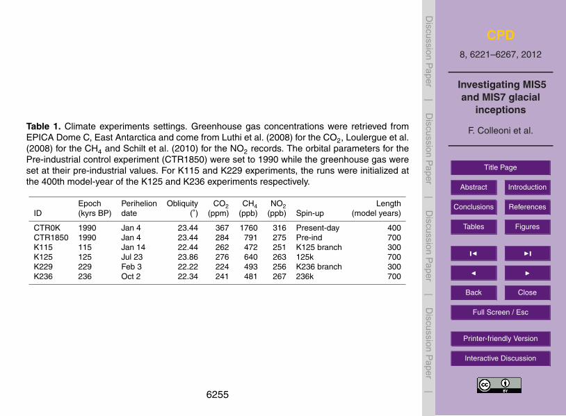
http://dx.doi.org/10.1029/2002GL015120

CPD8, 6221–6267, 2012


inceptions

F. Colleoni et al.

Title Page



Tables Figures

J I

J I

Back Close

Full Screen / Esc



Discussion

Paper

|D

iscussionP

aper|

Discussion

Paper

|D

iscussionP

aper|

Table 1. Climate experiments settings. Greenhouse gas concentrations were retrieved fromEPICA Dome C, East Antarctica and come from Luthi et al. (2008) for the CO2, Loulergue et al.(2008) for the CH4 and Schilt et al. (2010) for the NO2 records. The orbital parameters for thePre-industrial control experiment (CTR1850) were set to 1990 while the greenhouse gas wereset at their pre-industrial values. For K115 and K229 experiments, the runs were initialized atthe 400th model-year of the K125 and K236 experiments respectively.

Epoch Perihelion Obliquity CO2 CH4 NO2 LengthID (kyrs BP) date (◦) (ppm) (ppb) (ppb) Spin-up (model years)

CTR0K 1990 Jan 4 23.44 367 1760 316 Present-day 400CTR1850 1990 Jan 4 23.44 284 791 275 Pre-ind 700K115 115 Jan 14 22.44 262 472 251 K125 branch 300K125 125 Jul 23 23.86 276 640 263 125k 700K229 229 Feb 3 22.22 224 493 256 K236 branch 300K236 236 Oct 2 22.34 241 481 267 236k 700

6255





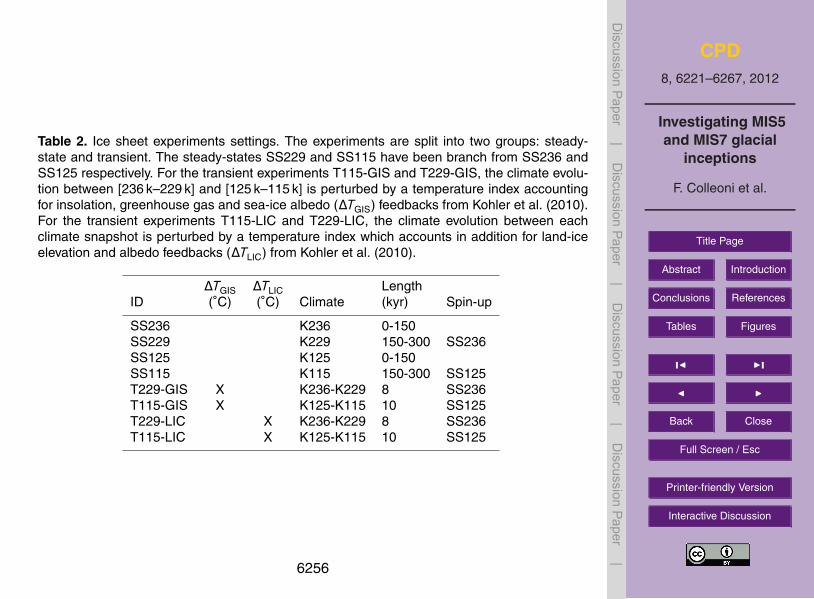
CPD8, 6221–6267, 2012


inceptions

F. Colleoni et al.

Title Page



Tables Figures

J I

J I

Back Close

Full Screen / Esc



Discussion

Paper

|D

iscussionP

aper|

Discussion

Paper

|D

iscussionP

aper|

Table 2. Ice sheet experiments settings. The experiments are split into two groups: steady-state and transient. The steady-states SS229 and SS115 have been branch from SS236 andSS125 respectively. For the transient experiments T115-GIS and T229-GIS, the climate evolu-tion between [236 k–229 k] and [125 k–115 k] is perturbed by a temperature index accountingfor insolation, greenhouse gas and sea-ice albedo (∆TGIS) feedbacks from Kohler et al. (2010).For the transient experiments T115-LIC and T229-LIC, the climate evolution between eachclimate snapshot is perturbed by a temperature index which accounts in addition for land-iceelevation and albedo feedbacks (∆TLIC) from Kohler et al. (2010).

∆TGIS ∆TLIC LengthID (◦C) (◦C) Climate (kyr) Spin-up

SS236 K236 0-150SS229 K229 150-300 SS236SS125 K125 0-150SS115 K115 150-300 SS125T229-GIS X K236-K229 8 SS236T115-GIS X K125-K115 10 SS125T229-LIC X K236-K229 8 SS236T115-LIC X K125-K115 10 SS125

6256





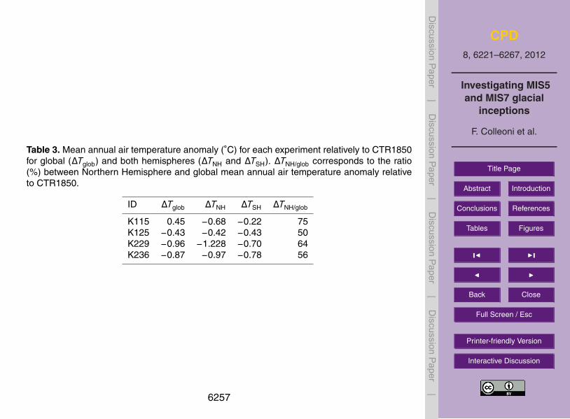
CPD8, 6221–6267, 2012


inceptions

F. Colleoni et al.

Title Page



Tables Figures

J I

J I

Back Close

Full Screen / Esc



Discussion

Paper

|D

iscussionP

aper|

Discussion

Paper

|D

iscussionP

aper|

Table 3. Mean annual air temperature anomaly (◦C) for each experiment relatively to CTR1850for global (∆Tglob) and both hemispheres (∆TNH and ∆TSH). ∆TNH/glob corresponds to the ratio(%) between Northern Hemisphere and global mean annual air temperature anomaly relativeto CTR1850.

ID ∆Tglob ∆TNH ∆TSH ∆TNH/glob

K115 0.45 −0.68 −0.22 75K125 −0.43 −0.42 −0.43 50K229 −0.96 −1.228 −0.70 64K236 −0.87 −0.97 −0.78 56

6257





CPD8, 6221–6267, 2012


inceptions

F. Colleoni et al.

Title Page



Tables Figures

J I

J I

Back Close

Full Screen / Esc



Discussion

Paper

|D

iscussionP

aper|

Discussion

Paper

|D

iscussionP

aper|

TIII

TIII

TII

TII

0 100 200 300

Time (kyrs BP)

ï�

ï�

0

�

An

tarc

tic 6

T (

°C

)

��200

220

��260

��

CO

2 (

pp

mv)��

500

600

700

&+��SSEY)

ï��

ï��

ï��

0

Se

a le

ve

l (m

)

ï��

ï��

ï��

0ï��5��0��5��0

ï��5��0��5��0

Be

nth

ic b

13C

(‰

) ��520

560

--$�LQVR��:

�P2)

��520

560

ï��

��

��

e*sin

( t

22

23

��

2EO��

0 100 200 300

70°S

65°N

D�

E�

F�

G�H�

I�

J�

MIS5 MIS7

1$':

$$%:

Fig. 1. Overview of the two last glacial cycles illustrated by different forcing and proxies. Fromtop to bottom: (a) obliquity (◦) and precession index (Laskar et al., 2004); (b) summer insolationat 65◦ N and 70◦ S (W m−2 Laskar et al., 2004); (c) benthic δ13C indicative of the changes insources of the North Atlantic deep waters formation at the Mediterranean latitudes (Martrat etal., 2007); (d) sea level reconstructions (m) from Bintaja and van de Wal (2008) (solid line),Siddall et al. (2003) (dashed line) and Waelbroeck et al. (2002) (dotted line); (e) atmosphericCH4 (ppbv) and CO2 (ppmv) concentrations from EPICA Dome C, East Antarctica (Loulergueet al., 2008; Luthi et al., 2008) and (f) EPICA Dome C, East Antarctica, temperature anomaly(◦C) relatively to present-day (Jouzel et al., 2007). Vertical grey bars indicate the time of theclimate snapshots simulations performed in this work. Termination II (TII) and Termination III(TIII) are indicated as well.

6258





CPD8, 6221–6267, 2012


inceptions

F. Colleoni et al.

Title Page



Tables Figures

J I

J I

Back Close

Full Screen / Esc



Discussion

Paper

|D

iscussionP

aper|

Discussion

Paper

|D

iscussionP

aper|

40

60

80

Latitu

des

0 1 2 3 4 5 6 7 8 9 10 11 12

236k − CTR1850 d.

−100 −80 −60 −40 −20 0 20 40 60 80 100

W/m2

40

60

80

Latitu

des

229k − CTR1850b.

40

60

80

Latitu

des

125k − CTR1850c.

40

60

80

Latitu

des

0 1 2 3 4 5 6 7 8 9 10 11 12

Months

115k − CTR1850a.

Fig. 2. Solar downward radiation anomaly at top of the atmosphere (W m−2) over the Northernhigh latitudes (40◦ N–90◦ N) between CTR1850 and the experiments described in Table 1.

6259





CPD8, 6221–6267, 2012


inceptions

F. Colleoni et al.

Title Page



Tables Figures

J I

J I

Back Close

Full Screen / Esc



Discussion

Paper

|D

iscussionP

aper|

Discussion

Paper

|D

iscussionP

aper|

−6

−4

−2

0

2

4

6

∆ T

(°C

)

112 116 120 124 128

Time (kyrs BP)

d.

−6

−4

−2

0

2

4

6

∆ T

(°C

)

220 224 228 232 236 240

Time (kyrs BP)

e.

−15

−10

−5

0

5

10∆

TG

R(°

C)

112 116 120 124 128

b.

−15

−10

−5

0

5

10

∆ T

GR(°

C)

220 224 228 232 236 240

c.

−20

−15

−10

−5

0

5

10

∆ T

GR(°

C)

0 20 40 60 80 100 120 140 160 180 200 220 240

Time (kyrs BP)

a.

Fig. 3. Temperature indices considered in this work: (a) temperature index ∆TGR (anomaly rel-ative to pre-industrial in ◦C) after Quiquet (2012). (b) and (c) ∆TGR (black) as in (a) divided intocontribution of combined orbitals, GHGs and sea-ice cover albedo feedbacks (orange) retrivedfrom Kohler et al. (2010) and contribution of additional land-ice albedo feedback (magenta).See Sect. 2.2.2 for more details on the calculations. Blue squares correspond to the simu-lated mean annual central Greenland temperature anomaly (relative to CTR1850) for each ofthe CESM experiments (Table 1). (d) and (e) Temperature indices ∆TGIS and ∆TLIC includingorbitals, GHGs and SIC (orange) and additionally accounting for land-ice albedo feedback (ma-genta) respectively. Temperature anomaly is relative to 125 kyr BP and 236 kyr BP values foreach inception period.

6260





CPD8, 6221–6267, 2012


inceptions

F. Colleoni et al.

Title Page



Tables Figures

J I

J I

Back Close

Full Screen / Esc



Discussion

Paper

|D

iscussionP

aper|

Discussion

Paper

|D

iscussionP

aper|

Fig. 4. Simulated air temperatures and precipitation anomalies relatively to pre-industrial con-trol run CTR1850 in the Northern Hemisphere 30◦ N to 90◦ N. Top row (a) to (d): simulatedmean summer air temperature anomaly (June-July-August, JJA) in ◦C calculated as the differ-ence between each experiment and CTR1850. Bottom row (e) to (h): simulated mean annualprecipitation anomaly calculated as the ratio between each experiment and CTR1850 (dimen-sionless).

6261





CPD8, 6221–6267, 2012


inceptions

F. Colleoni et al.

Title Page



Tables Figures

J I

J I

Back Close

Full Screen / Esc



Discussion

Paper

|D

iscussionP

aper|

Discussion

Paper

|D

iscussionP

aper|

Fig. 5. Simulated residence time (days/year) of snow cover for each climate experiment,(a) K125, (b). K115, (c) K236 and (d) K229. Snow cover is considered permanent when resi-dence time is equal or larger than 365 days (dark blue). Values are shown from 360 days onlyto increase the legibility of the figure.

6262





CPD8, 6221–6267, 2012


inceptions

F. Colleoni et al.

Title Page



Tables Figures

J I

J I

Back Close

Full Screen / Esc



Discussion

Paper

|D

iscussionP

aper|

Discussion

Paper

|D

iscussionP

aper|

Fig. 6. Bias in temperature an precipitation in the Northern Hemisphere in the low resolutionpresent-day anthropogenic run CTR0k (Table 1) as evidenced by NCEP reanalysis air tem-perature (Kalnay et al., 1996) and GPCP precipitation dataset (Adler et al., 2003). (a) and (b)simulated winter (DJF) and summer (JJA) air temperature anomaly (◦C) between CTR0k andNCEP reanalysis. (c) and (d) precipitation anomaly ratio (dimensionless) between CTR0k andGPCP precipitation dataset.

6263





CPD8, 6221–6267, 2012


inceptions

F. Colleoni et al.

Title Page



Tables Figures

J I

J I

Back Close

Full Screen / Esc



Discussion

Paper

|D

iscussionP

aper|

Discussion

Paper

|D

iscussionP

aper|

Fig. 7. Simulated ice thickness in meters for each of the steady-state experiment SS125 (a),SS115 (b), SS236 (c) and SS229 (d). See Table 2 for details. Simulated total ice volume valuesfor each experiment are expressed in meters Sea Level Equivalent (SLE) and are reported ineach frame.

6264





CPD8, 6221–6267, 2012


inceptions

F. Colleoni et al.

Title Page



Tables Figures

J I

J I

Back Close

Full Screen / Esc



Discussion

Paper

|D

iscussionP

aper|

Discussion

Paper

|D

iscussionP

aper|

−60

−40

−20

0

20R

ela

tive S

ea L

evel (m

.a.s

.l.)

110 115 120 125 130

Time (kyrs BP)

a.

−80

−60

−40

−20

0

20

Rela

tive S

ea L

evel (m

.a.s

.l.)

225 230 235 240

Time (kyrs BP)

b.

Fig. 8. Ice volume of steady-state experiments (blue and red dots) and of transient experi-ments (orange and magenta squares) expressed in relative sea-level (m a.s.l.) for MIS5 glacialinception period (a) and MIS7 inception period (b). Orange squares correspond to transientexperiments T115-GIS and T229-GIS ice volume evolution, forced using ∆TGIS index account-ing for orbitals, GHGs and SIC. Magenta squares corresponds to T115-LIC and T229-LIC icevolume evolution, forced using ∆TLIC index additionally accounting for land-ice elevation andalbedo feedbacks. Simulated values are compared to various sea-level reconstructions: Wael-broeck et al. (2002) (black); Siddall et al. (2003) (blue); Shackleton (2000) (brown); Bintaja etal. (2005) (red) and Lea et al. (2002) (orange).

6265





CPD8, 6221–6267, 2012


inceptions

F. Colleoni et al.

Title Page



Tables Figures

J I

J I

Back Close

Full Screen / Esc



Discussion

Paper

|D

iscussionP

aper|

Discussion

Paper

|D

iscussionP

aper|

Fig. 9. Simulated ice thickness in meters for each of the transient experiment T115-GIS (a),T115-LIC (b), T229-GIS (c) and T229-LIC (d). At the bottom of each frame is indicated thefeedbacks included into the temperature indices used to modulate the transient experiments.

6266





CPD8, 6221–6267, 2012


inceptions

F. Colleoni et al.

Title Page



Tables Figures

J I

J I

Back Close

Full Screen / Esc



Discussion

Paper

|D

iscussionP

aper|

Discussion

Paper

|D

iscussionP

aper|

0

2

4

6

Ice

sh

ee

t a

rea

(1

06 k

m2)

116 118 120 122 124

Time (kyrs BP)

d.

0

2

4

6

Ice

sh

ee

t a

rea

(1

06 k

m2)

230 232 234 236

Time (kyrs BP)

e.

0

2

4

6

8

10

12

14

16

18

20

Ice

vo

lum

e (

m S

LE

)

115 120 125

b.Eurasia − GIS

North America − GIS

Eurasia − LIC

North American − LIC

0

2

4

6

8

10

12

14

16

18

20

Ice

Vo

lum

e(m

SL

E)

230 235

c.

0.0

0.5

1.0

1.5

2.0

Exp

an

sio

n r

ate

(1

06 k

m2/k

yr)

0.0 0.5 1.0 1.5 2.0

Accumulation rate (m SLE/kyr)

a.

Fig. 10. Simulated time evolution of ice volume (b and c) and ice-covered areas (d and e) foreach transient experiment T115-GIS, T115-LIC, T229-GIS and T229-LIC, and separated intoNorth American (blue) and Eurasian (red) ice sheets evolution. GIS and LIC refer to temper-ature indices ∆TGIS and ∆TLIC respectively. Finally, top frame shows the relationship betweenthe expansion rates (106 km2 kyr−1) and the accumulation rates (m SLE kyr−1) of Eurasian (red)and North American (blue) ice sheets for each transient experiments T115-GIS (dots), T115-LIC (squares), T229-GIS (triangles) and T229-LIC (diamonds).

6267





Modelling Northern Hemisphere ice sheets distribution during MIS5 and MIS7 glacial inceptions

Documents

Transcript of Modelling Northern Hemisphere ice sheets distribution during MIS5 and MIS7 glacial inceptions