1 The VISTA Hemisphere Survey SMP
26
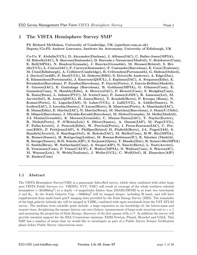
ESO Survey Management Plan Form:VISTA Hemisphere Survey Phase 1 1 The VISTA Hemisphere Survey SMP PI: Richard McMahon, University of Cambridge, UK ([email protected]) Deputy/Co-PI: Andrew Lawrence, Institute for Astronomy, University of Edinburgh, UK Co-I’s: F. Abdalla(UCL), D. Alexander(Durham), J. Alfonso(IAC), C. Bailer-Jones(MPIA), M. Balcells(IAC), X. Barcons(Santander), D. Barrado y Navascues(Madrid), V. Belokurov(Cam), E. Bell(MPIA), N. Ben´ ıtez(Granada), J. Bouvier(Grenoble), M. Bremer(Bristol), S. Bri- dle(UCL), L. Cairos(IAC), F. Carrera(Santander), F. Castander(Barcelona), E. Caux(Toulouse), M. Cioni(Edinburgh), A. Collister(Cambridge), R. Crittenden(Portsmouth), G. Dalton(Oxford), J. Davies(Cardiff), P. Doel(UCL), M. Doherty(ESO), S. Driver(St Andrews), A. Edge(Dur), E. Edmundson(Portsmouth), J. Emerson(QMUL), J. Espinosa(IAC), A. Ferguson(Edin), E. Fern´ andez(Barcelona), P. Fosalba(Barcelona), P. Garcia(Porto), J. Garc´ ıa-Bellido(Madrid), F. Garzon(IAC), E. Gazta˜ naga (Barcelona), B. Goldman(MPIA), G. Gilmore(Cam), E. Gonzalez(Cam), N. Hambly(Edin), A. Hererro(IAC), P. Hewett(Cam), S. Hodgkin(Cam), R. Ibata(Stras), L. Infante(PUC), M. Irwin(Cam), P. James(LJMU), R. Jameson(Lei), M. Jarvis(Oxf), B. Jones(QMUL), H. Jones(Herts), T. Kendall(Herts), P. Kroupa (Bonn), N. Kumar(Porto), G. Lagache(IAS), O. Lahav(UCL), J. Lalli(UCL), A. Liddle(Sussex), N. Lodieu(IAC), J. Loveday(Sussex), P. Lucas(Herts), R. Maartens(Ports), A. Manchado(IAC), R. Mann(Edin), E. Martin(IAC), N. Martin(Stras), M. Mart´ ınez(Barcelona), J. Maza(U.Chile), R. Miquel(Barcelona), J. Miralda-Escud´ e(Barcelona), M. Moles(Granada), M. Molla(Madrid), J-L Monin(Grenoble), E. Moraux(Grenoble), C. Munoz-Tunon(IAC), T. Naylor(Exeter), R. Nichol(Ports), P. O’Brien(Leic) S. Oliver(Sussex), A. Omont(IAP), M. Page(UCL), F. Palla(Arcetri), J. Peacock(Edin), W. Percival(Ports), I. Perez-Fournon(IAC), C. Per- oux(ESO), P. Petitjean(IAP), S. Phillips(Bristol) D. Pinfield(Herts), J-L. Puget(IAS), S. Randich(Arcetri), S. Rawlings(Oxf), R. Rebolo(IAC), M. Riello(Cam), H-W. Rix(MPIA), K. Romer(Sussex), H. Rottgering(Leiden), M. Rowan-Robinson(IC), E. S´ anchez (Madrid), R. Savage(Sussex), R-D. Scholz(AIP), S. Serjeant(Open), T. Shanks(Dur), R. Somerville(MPIA) G. Smith(Birm), W. Sutherland(Cam), A. Swope(AIP), N. Tanvir(Herts), L. Testi(Arcetri), B. Venemans(Cam), P. Viana(CAUP), F. Walter(MPIA), N. Walton(Cam), S. Warren(IC), M. Watson(Leic), N. Webb(Toulouse), J. Weller(UCL), C. Wolf(Oxf), H. Zinnecker(AIP) D. Zucker(Cam) 1.1 Abstract The VISTA Hemisphere Survey(VHS) is a panoramic Infra-Red survey, which when combined with other large area VISTA Public Surveys (i.e. VIKING, VVV, VMC) will result in coverage of the whole southern celestial hemisphere (∼20,000deg 2 ) to a depth ∼4 magnitudes fainter than 2MASS/DENIS in at least two wavebands J and K s . In the South Galactic Cap, ∼5000deg 2 will be imaged deeper, including H band, and will have supplemental deep multi-band grizY imaging data provided by the Dark Energy Survey (DES). The remainder of the high galactic latitude sky will be imaged in YJHK s combined with ugriz wavebands from the VST ATLAS survey. The medium term scientific goals include: a huge expansion in our knowledge of; the lowest-mass and nearest stars; deciphering the merger history our own Galaxy; measurement of large-scale structure out to z 1 and measuring the properties of Dark Energy; discovery of the first quasar with z>7. In addition the survey will provide essential support for the ESA Cornerstone missions; XMM-Newton, Planck, Herschel and GAIA. This SMP has a number of issues that we would like to investigate as part of a Public Survey Science Verification phase before Public Survey observations start. ESO-USD ([email protected]) Version 1.0; 05 June 07 page 1 of 26
-
Upload
independent -
Category
Documents
-
view
0 -
download
0
Transcript of 1 The VISTA Hemisphere Survey SMP
ESO Survey Management Plan Form:VISTA Hemisphere Survey Phase 1
1 The VISTA Hemisphere Survey SMP
PI: Richard McMahon, University of Cambridge, UK ([email protected])Deputy/Co-PI: Andrew Lawrence, Institute for Astronomy, University of Edinburgh, UK
Co-I’s: F. Abdalla(UCL), D. Alexander(Durham), J. Alfonso(IAC), C. Bailer-Jones(MPIA),M. Balcells(IAC), X. Barcons(Santander), D. Barrado y Navascues(Madrid), V. Belokurov(Cam),E. Bell(MPIA), N. Benıtez(Granada), J. Bouvier(Grenoble), M. Bremer(Bristol), S. Bri-dle(UCL), L. Cairos(IAC), F. Carrera(Santander), F. Castander(Barcelona), E. Caux(Toulouse),M. Cioni(Edinburgh), A. Collister(Cambridge), R. Crittenden(Portsmouth), G. Dalton(Oxford),J. Davies(Cardiff), P. Doel(UCL), M. Doherty(ESO), S. Driver(St Andrews), A. Edge(Dur),E. Edmundson(Portsmouth), J. Emerson(QMUL), J. Espinosa(IAC), A. Ferguson(Edin), E.Fernandez(Barcelona), P. Fosalba(Barcelona), P. Garcia(Porto), J. Garcıa-Bellido(Madrid),F. Garzon(IAC), E. Gaztanaga (Barcelona), B. Goldman(MPIA), G. Gilmore(Cam), E.Gonzalez(Cam), N. Hambly(Edin), A. Hererro(IAC), P. Hewett(Cam), S. Hodgkin(Cam),R. Ibata(Stras), L. Infante(PUC), M. Irwin(Cam), P. James(LJMU), R. Jameson(Lei), M.Jarvis(Oxf), B. Jones(QMUL), H. Jones(Herts), T. Kendall(Herts), P. Kroupa (Bonn), N.Kumar(Porto), G. Lagache(IAS), O. Lahav(UCL), J. Lalli(UCL), A. Liddle(Sussex), N.Lodieu(IAC), J. Loveday(Sussex), P. Lucas(Herts), R. Maartens(Ports), A. Manchado(IAC),R. Mann(Edin), E. Martin(IAC), N. Martin(Stras), M. Martınez(Barcelona), J. Maza(U.Chile),R. Miquel(Barcelona), J. Miralda-Escude(Barcelona), M. Moles(Granada), M. Molla(Madrid),J-L Monin(Grenoble), E. Moraux(Grenoble), C. Munoz-Tunon(IAC), T. Naylor(Exeter),R. Nichol(Ports), P. O’Brien(Leic) S. Oliver(Sussex), A. Omont(IAP), M. Page(UCL),F. Palla(Arcetri), J. Peacock(Edin), W. Percival(Ports), I. Perez-Fournon(IAC), C. Per-oux(ESO), P. Petitjean(IAP), S. Phillips(Bristol) D. Pinfield(Herts), J-L. Puget(IAS), S.Randich(Arcetri), S. Rawlings(Oxf), R. Rebolo(IAC), M. Riello(Cam), H-W. Rix(MPIA),K. Romer(Sussex), H. Rottgering(Leiden), M. Rowan-Robinson(IC), E. Sanchez (Madrid),R. Savage(Sussex), R-D. Scholz(AIP), S. Serjeant(Open), T. Shanks(Dur), R. Somerville(MPIA)G. Smith(Birm), W. Sutherland(Cam), A. Swope(AIP), N. Tanvir(Herts), L. Testi(Arcetri),B. Venemans(Cam), P. Viana(CAUP), F. Walter(MPIA), N. Walton(Cam), S. Warren(IC),M. Watson(Leic), N. Webb(Toulouse), J. Weller(UCL), C. Wolf(Oxf), H. Zinnecker(AIP)D. Zucker(Cam)
1.1 Abstract
The VISTA Hemisphere Survey(VHS) is a panoramic Infra-Red survey, which when combined with other largearea VISTA Public Surveys (i.e. VIKING, VVV, VMC) will result in coverage of the whole southern celestialhemisphere (∼20,000deg2) to a depth ∼4 magnitudes fainter than 2MASS/DENIS in at least two wavebandsJ and Ks. In the South Galactic Cap, ∼5000deg2 will be imaged deeper, including H band, and will havesupplemental deep multi-band grizY imaging data provided by the Dark Energy Survey (DES). The remainderof the high galactic latitude sky will be imaged in YJHKs combined with ugriz wavebands from the VST ATLASsurvey. The medium term scientific goals include: a huge expansion in our knowledge of; the lowest-mass andnearest stars; deciphering the merger history our own Galaxy; measurement of large-scale structure out to z ' 1and measuring the properties of Dark Energy; discovery of the first quasar with z>7. In addition the survey willprovide essential support for the ESA Cornerstone missions; XMM-Newton, Planck, Herschel and GAIA. ThisSMP has a number of issues that we would like to investigate as part of a Public Survey Science Verificationphase before Public Survey observations start.
ESO-USD ([email protected]) Version 1.0; 05 June 07 page 1 of 26
ESO Survey Management Plan Form:VISTA Hemisphere Survey Phase 1
2 Survey Observing Strategy
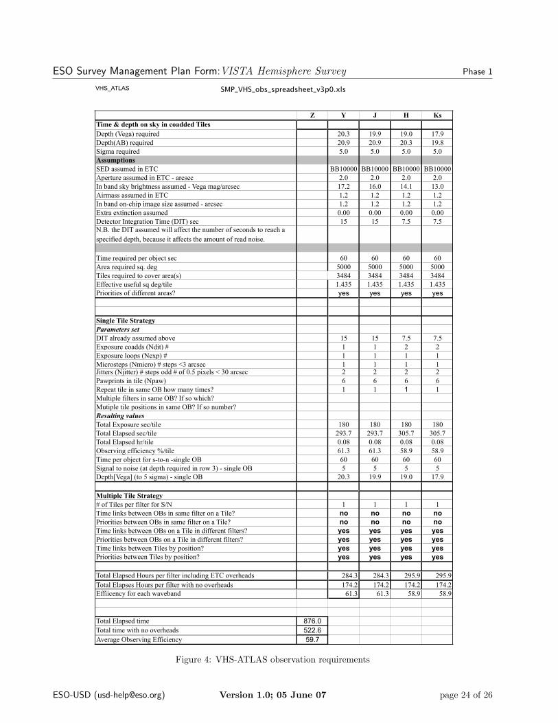
This section should be read in conjunction with the enclosed Excel spreadsheet and the three figures that showthe main tabular data contained with this Excel spreadsheet. There is one tabular figure for each of the threeVHS survey components described below.
2.1 Scheduling requirements
The VHS survey is divided into 3 components for survey planning and management and purposes, based ontheir common OB structures. These components in alphabetic order are:
• VHS-ATLAS (∼5000 deg2); consists of two regions of sky, one in the north galactic cap(NGC; ∼2500deg2) and the second in the south galactic cap ( SGC;∼2500deg2) to be observed in YJHKs for 60secs perwaveband.
• VHS-DES (∼4500 deg2); a contiguous region of sky in the SGC to be observed in JHKs for 120secs perwaveband.
• VHS-GPS (∼8200 deg2); A region of lower galactic latitude which we define as the VHS Galactic PlaneSurvey(GPS) with 5◦ < |b| < 30◦ (∼8200 deg2); excluding the VVV and VMC regions; to be observed inJ and K for 60secs per waveband.
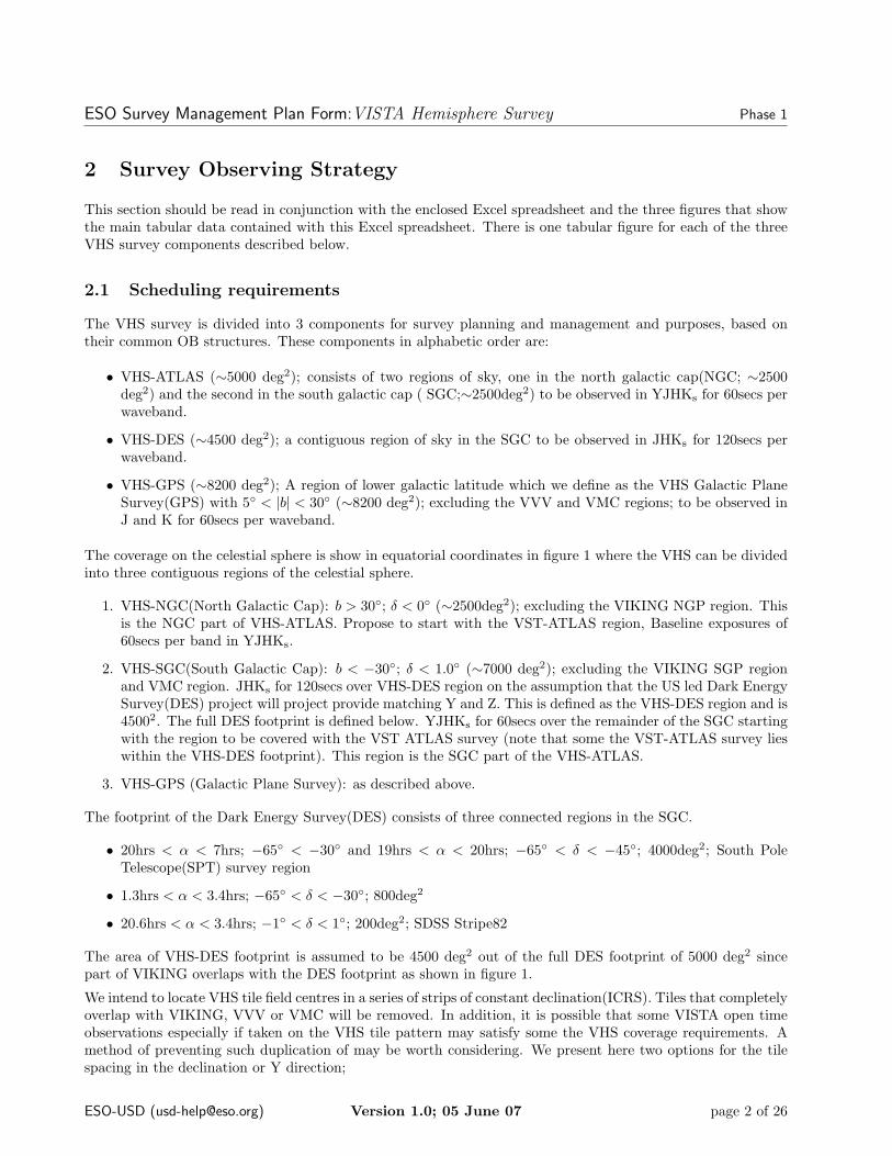
The coverage on the celestial sphere is show in equatorial coordinates in figure 1 where the VHS can be dividedinto three contiguous regions of the celestial sphere.
1. VHS-NGC(North Galactic Cap): b > 30◦; δ < 0◦ (∼2500deg2); excluding the VIKING NGP region. Thisis the NGC part of VHS-ATLAS. Propose to start with the VST-ATLAS region, Baseline exposures of60secs per band in YJHKs.
2. VHS-SGC(South Galactic Cap): b < −30◦; δ < 1.0◦ (∼7000 deg2); excluding the VIKING SGP regionand VMC region. JHKs for 120secs over VHS-DES region on the assumption that the US led Dark EnergySurvey(DES) project will project provide matching Y and Z. This is defined as the VHS-DES region and is45002. The full DES footprint is defined below. YJHKs for 60secs over the remainder of the SGC startingwith the region to be covered with the VST ATLAS survey (note that some the VST-ATLAS survey lieswithin the VHS-DES footprint). This region is the SGC part of the VHS-ATLAS.
3. VHS-GPS (Galactic Plane Survey): as described above.
The footprint of the Dark Energy Survey(DES) consists of three connected regions in the SGC.
• 20hrs < α < 7hrs; −65◦ < −30◦ and 19hrs < α < 20hrs; −65◦ < δ < −45◦; 4000deg2; South PoleTelescope(SPT) survey region
• 1.3hrs < α < 3.4hrs; −65◦ < δ < −30◦; 800deg2
• 20.6hrs < α < 3.4hrs; −1◦ < δ < 1◦; 200deg2; SDSS Stripe82
The area of VHS-DES footprint is assumed to be 4500 deg2 out of the full DES footprint of 5000 deg2 sincepart of VIKING overlaps with the DES footprint as shown in figure 1.
We intend to locate VHS tile field centres in a series of strips of constant declination(ICRS). Tiles that completelyoverlap with VIKING, VVV or VMC will be removed. In addition, it is possible that some VISTA open timeobservations especially if taken on the VHS tile pattern may satisfy some the VHS coverage requirements. Amethod of preventing such duplication of may be worth considering. We present here two options for the tilespacing in the declination or Y direction;
ESO-USD ([email protected]) Version 1.0; 05 June 07 page 2 of 26
ESO Survey Management Plan Form:VISTA Hemisphere Survey Phase 1
Figure 1: Overview of VHS and other VISTA survey coverage(Best viewed in colour)
(i) In the first which is a conservative strategy we propose to use 59.0 arcmin (0.983◦) in declination or Ydirection as proposed by VIKING which is driven by the footprint of the VST. Since it is intended tocombine VISTA and VST data having a grid pattern that matches in at least one axis aids scientificexploitation. This tiling strategy also results in the minimisation of overlap of partial tiles in observingfootprint for VHS and VIKING. The above strategy will result in an overlap of 2 arcmin between stripes atthe full VISTA depth after adjacent VHS stripes have been observed. This overlap will be used for globalastrometric and photometric re-calibration. It will also minimise the number of astronomical objects thatare chopped in half by the edges of the VISTA field of view and window pane effects that is often observedin mosaiced data. The RA or X spacing will be 1.46◦ which will give 1arcmin overlap between neighbouringVISTA tiles in the same declination stripe. The unique area for this tiling strategy is 1.46◦ × 0.983◦ =1.435deg2. This total time required using this strategy is shown in table 1. A more detailed breakdownin terms of the OB design is given in the enclosed spreadsheet. The main tables from the spreadsheet areshown in Appendix 1.
(ii) In the second case we assume a zero tile overlap strategy and assume an effective tile footprint of 1.636deg2.This total time required using this strategy is shown in table 2
(iii) Since submitting the first version of the VHS SMP(v0.5) we have investigated the overlap strategy used byother surveys. For SDSS and 2MASS the overlap is 1’ along edges. The UKIDSS LAS uses an minimumoverlap of 3% which is 25arcsec. In practice we need to determine the number of stars objects that wouldbe detected at S/N of 10 within the overlap regions for each chip between adjacent tiles. Also there tendto be larger systematic uncertainties near the boundaries of detectors. A pragmatic approach based onother similar surveys is to use an overlap of 30”. For this strategy the effective tile size is 1.614deg2
and the total time required with this tiling strategy is 3025hours. We will also need evaluate whether toobserve with the default PA=0 or PA=90 since observations at PA=90 when combined with linked OB indeclination strips will minimise the difference in observing conditions in the half-chip overlap regions.
The total time required for VHS assuming the ’conservative’ tiling strategy of 1.435deg2 and overheads fromthe ETC is 3402 hours. Thus the total time has increased from 3107 hours to 3402 hours as defined in Table 7
ESO-USD ([email protected]) Version 1.0; 05 June 07 page 3 of 26
ESO Survey Management Plan Form:VISTA Hemisphere Survey Phase 1
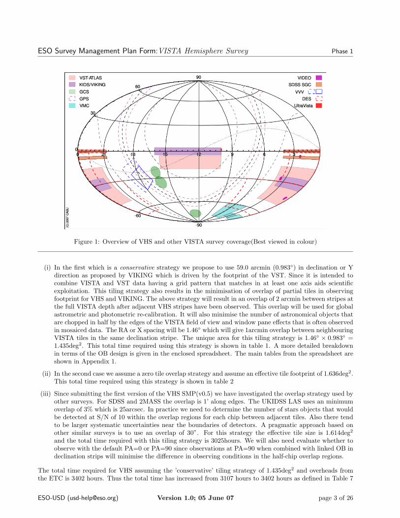
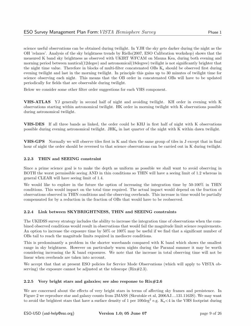
Figure 2: Star and galaxy counts from 2MASS(Skrutskie et al, 2006)
in the Sep, 2006 PSP-OPC submission due to the following factors:
1. increase in overheads due to the inclusion of a jitter in the VHS-ATLAS and VHS-GPS so that all skyregions are sampled by more than one independent pixel even in the presence of bad pixels.
2. overhead increase due to an increase in the number of DITS in H and K to avoid detector saturation.
3. we have changed the effective tile size from 1.50 deg2 to 1.435deg2 as defined above.
The increases caused by these have been offset by reducing the area of the VHS-ATLAS survey from 6000 deg2
to 5000 deg2. This is possible because, the PSP-OPC Sep, 2006 submission had some double counting betweenthe footprints of VIKING, VHS-ATLAS and VHS-DES.
In the case of a ’zero overlap’ strategy the total time required is 2986 hours at a cost in uniformity of thesurvey data. In particular in the inter-tile overlap region the resultant data that would be co-added would havedifferent seeing, sky transparency, sky brightness and epoch of observations. This inter-tile overlap region hasa width of 5.5arcmin at the top and bottom i.e. north and south edges in the default PA=0 orientation. Thiswould effect ∼10% of the sky coverage. Note that a PA=90 may be used in VHS.
The control of systematic uncertainties is an important science requirement for the large scale structure andDark Energy science case which is the primary science driver for the VHS-DES region. We would thereforefavour the conservative tiling strategy for this region. We request that the optimal tiling strategy in investigatedduring a VHS Science Verification phase. One intermediate tiling strategy would be to have a 0.5-1.0arcminregion around all 4 sides that has 100% exposure overlap. A related factor is that bad pixels and other processingsteps tend to more unreliable near the edges. These need on-sky determinations.
VHS has fields over the full RA range when all three components are considered so that the survey can becarried out in all months of the year. VHS also has a fields over the full range of declinations so that fieldsshould be available in the presence of all wind direction constraints. Due to the wide declination range at allRA, there should also always be fields that are sufficiently far from the ecliptic that moon avoidance does notrestrict scheduling.
In Table ?? we show the RA distribution of the priority of each survey component. In addition we shall supplyfiner grained priorities for specific regions of sky within each survey e.g. by declination stripe for the VHS-DESand VHS-ATLAS components or galactic l, b in the case of VHS-GPS with seeing limits that take into accountstellar confusion.
ESO-USD ([email protected]) Version 1.0; 05 June 07 page 4 of 26

ESO Survey Management Plan Form:VISTA Hemisphere Survey Phase 1
Table 1: VHS total time per waveband assuming an effective tile size of 1.435 deg2
Sub-Survey deg2 Y J H K TotalVHS-ATLAS 5000 284 284 296 296 1160VHS-DES 4500 - 423 434 434 1290VHS-GPS 8200 - 466 - 485 951
Total Elapsed 17,700 284 1074 729 1215 3402Total Science 174 774 488 774 2209Efficiency(%) 61 66 67 64 65
Notes: (i) We have assumed that ATLAS is extended beyond 4500deg2 current 3 year goals and a total area for VHS-ATLAS of
5000deg2. (iI) DES will cover 5000deg2 but we assume that 500deg2 overlaps with VIKING. (iii) We have recomputed the
combined area covered by VHS-DES and VHS-ATLAS and it is 9,500 deg2 compared with 10,500 deg2 in the original proposal.
We have therefore reduced the VHS-ATLAS footprint from 6000 deg2 to 5,000 deg2. Some of the VST-ATLAS region lies within
the VHS-DES region.
Table 2: VHS total time per waveband assuming an effective tile size of 1.636 deg2
Sub-Survey deg2 Y J H K TotalVHS-ATLAS 5000 249 249 260 260 1018VHS-DES 4500 371 381 381 1132VHS-GPS 8200 409 426 835
Total Elapsed 17,700 249 1030 640 1066 2986Total Science 153 679 428 679 1939Efficiency(%) 61 66 67 64 65
Notes: see notes to table 1.
Following the PSP recommendation we propose to complete the survey in 10 periods over 5 years. In Table 4we summarize the time required per period. Initially we ask for an evenly divided spread in time in each period.It is possible that this may need amending after a few periods have passed. The distribution of observing timerequest with period over the first 10 Periods is given in Table 4 assuming a total of 10 periods for the wholesurvey. The original submission assumed a survey start in P79. Here we assume a start in P80( Oct’07-Mar’08).
Each tile will be observed only once in each waveband. For all the surveys we require that a minimum of twowavebands are observed with a time interval between bands of no more that 30 minutes so that the effects ofshort term variability are minimised and that moving objects can be identified. Therefore the separate wavebands will be observed via concatenated OBs as follows:
• VHS-ATLAS; Y and J concatenated; H and K concatenated [same strategy as UKIDSS LAS]
• VHS-DES; H and K concatenated and J unconcatenated or all three concatenated or with a goal to observewithin 1hr of the concatenated HK OBs.
• VHS-GPS; J and K concatenated OBs
Another requirement on OB links is that in the IR, the sky has to subracted and we will require a minimum of2 tiles in order to determine the sky that has to be subtracted from each observation. Thus in Y, J H and K wewill need to concatenate two tiles in each waveband. The elapsed time per tile per waveband is shown in Table5. The total time, for a group of concatenated OBs ranges from 972 secs for the DES J band observations,1200secs for ATLAS and GPS to 1792 secs for the DES HK concatenated observations of two adjacent tiles.
In the case of the VHS-ATLAS survey concatenated YJ Obs will be observed during grey/dark time andconcatenated HK OBs will be observed during any observing conditions. The concatenated OBs should be
ESO-USD ([email protected]) Version 1.0; 05 June 07 page 5 of 26
ESO Survey Management Plan Form:VISTA Hemisphere Survey Phase 1
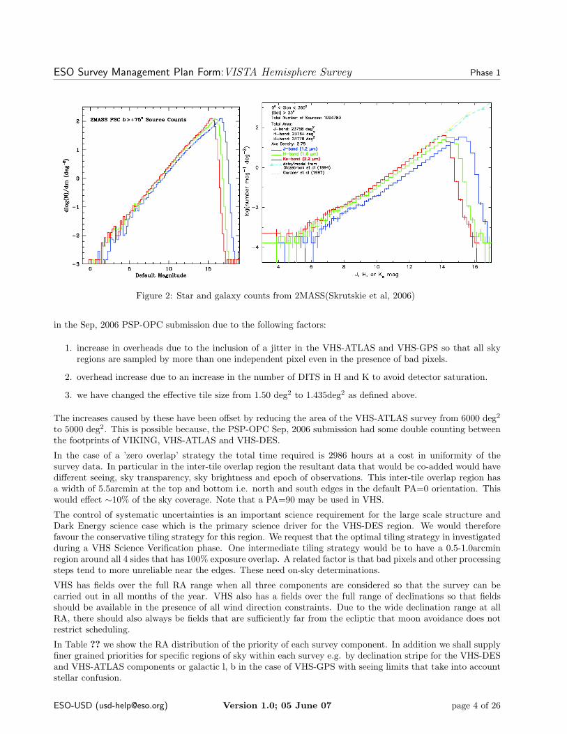
Table 3: VHS Survey Top Level survey region Priorities by RAPriority
RA 1 2 300-01 DES ATLAS01-02 DES ATLAS02-03 DES ATLAS03-04 DES ATLAS04-05 DES ATLAS05-06 DES ATLAS GPS06-07 DES ATLAS GPS07-08 GPS08-09 GPS09-10 ATLAS GPS10-11 ATLAS GPS11-12 ATLAS GPS12-13 ATLAS GPS13-14 ATLAS GPS14-15 ATLAS GPS15-16 ATLAS GPS16-17 GPS17-18 GPS18-19 GPS19-20 GPS20-21 DES ATLAS GPS21-22 DES ATLAS GPS22-23 DES ATLAS23-24 DES ATLAS
Notes: These are the top level priorities between the VHS survey components. Additional finer grained priorities as a function of
declination and/or galactic latitude are also planned.
observed ideally within 1 month. A goal would to be observe all wavebands in a tile within 6 months otherwiselong term variability will reduce the scientific value of the multi-colour data.
Other observing priority drivers that may require intervention during an observing period are caused by thelink with the VST ATLAS survey. We would like to increase the OB priority for VHS tiles that are for regionsof sky that have already been observed by VST-ATLAS. These priorities will be updated at the start of eachobserving period but it may be desirable to alter OB priorities during an obserging period on a monthly basis.
2.2 Observing requirements
The science goals require that we cover the whole southern sky in a minimum of two wavebands and ZYJHKs
and over the high galactic latitude sky. In the first instance Z will come from the VST ATLAS survey and/orthe CTIO DES project. The DES project will also provide Y band data over the DES footprint. We assume1.2” seeing as measured on VIRCAM images at the VISTA focal plane in each filter and 5sigma detection limitsin a 2arcsec diameter aperture. Baseline exposure times of 60 seconds in all bands are assumed except over theDES region where 120secs in JHKs are used.
Because of potential variables we ideally wish to get at least two filters observed within 30 minutes of each otherby having them in concatenated OBs. For example studies of the variability in a 4Myr-old OB association by
ESO-USD ([email protected]) Version 1.0; 05 June 07 page 6 of 26
ESO Survey Management Plan Form:VISTA Hemisphere Survey Phase 1
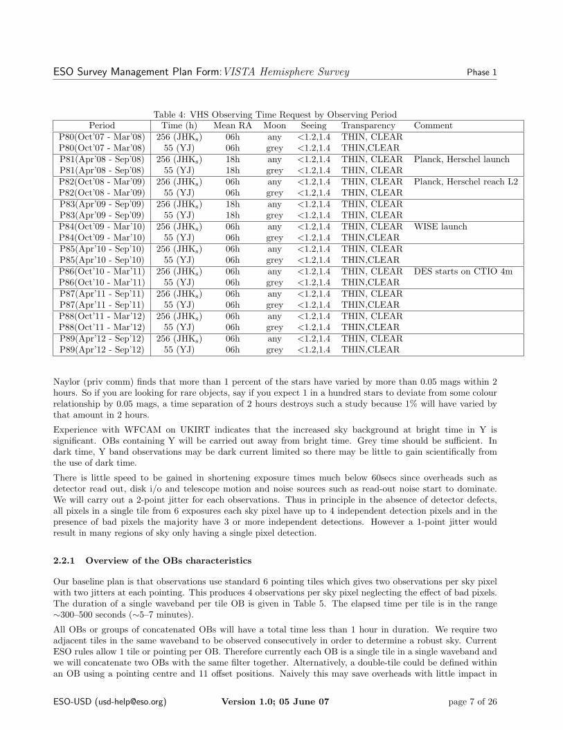
Table 4: VHS Observing Time Request by Observing PeriodPeriod Time (h) Mean RA Moon Seeing Transparency Comment
P80(Oct’07 - Mar’08) 256 (JHKs) 06h any <1.2,1.4 THIN, CLEARP80(Oct’07 - Mar’08) 55 (YJ) 06h grey <1.2,1.4 THIN,CLEARP81(Apr’08 - Sep’08) 256 (JHKs) 18h any <1.2,1.4 THIN, CLEAR Planck, Herschel launchP81(Apr’08 - Sep’08) 55 (YJ) 18h grey <1.2,1.4 THIN, CLEARP82(Oct’08 - Mar’09) 256 (JHKs) 06h any <1.2,1.4 THIN, CLEAR Planck, Herschel reach L2P82(Oct’08 - Mar’09) 55 (YJ) 06h grey <1.2,1.4 THIN, CLEARP83(Apr’09 - Sep’09) 256 (JHKs) 18h any <1.2,1.4 THIN, CLEARP83(Apr’09 - Sep’09) 55 (YJ) 18h grey <1.2,1.4 THIN, CLEARP84(Oct’09 - Mar’10) 256 (JHKs) 06h any <1.2,1.4 THIN, CLEAR WISE launchP84(Oct’09 - Mar’10) 55 (YJ) 06h grey <1.2,1.4 THIN,CLEARP85(Apr’10 - Sep’10) 256 (JHKs) 06h any <1.2,1.4 THIN, CLEARP85(Apr’10 - Sep’10) 55 (YJ) 06h grey <1.2,1.4 THIN,CLEARP86(Oct’10 - Mar’11) 256 (JHKs) 06h any <1.2,1.4 THIN, CLEAR DES starts on CTIO 4mP86(Oct’10 - Mar’11) 55 (YJ) 06h grey <1.2,1.4 THIN,CLEARP87(Apr’11 - Sep’11) 256 (JHKs) 06h any <1.2,1.4 THIN, CLEARP87(Apr’11 - Sep’11) 55 (YJ) 06h grey <1.2,1.4 THIN,CLEARP88(Oct’11 - Mar’12) 256 (JHKs) 06h any <1.2,1.4 THIN, CLEARP88(Oct’11 - Mar’12) 55 (YJ) 06h grey <1.2,1.4 THIN,CLEARP89(Apr’12 - Sep’12) 256 (JHKs) 06h any <1.2,1.4 THIN, CLEARP89(Apr’12 - Sep’12) 55 (YJ) 06h grey <1.2,1.4 THIN,CLEAR
Naylor (priv comm) finds that more than 1 percent of the stars have varied by more than 0.05 mags within 2hours. So if you are looking for rare objects, say if you expect 1 in a hundred stars to deviate from some colourrelationship by 0.05 mags, a time separation of 2 hours destroys such a study because 1% will have varied bythat amount in 2 hours.
Experience with WFCAM on UKIRT indicates that the increased sky background at bright time in Y issignificant. OBs containing Y will be carried out away from bright time. Grey time should be sufficient. Indark time, Y band observations may be dark current limited so there may be little to gain scientifically fromthe use of dark time.
There is little speed to be gained in shortening exposure times much below 60secs since overheads such asdetector read out, disk i/o and telescope motion and noise sources such as read-out noise start to dominate.We will carry out a 2-point jitter for each observations. Thus in principle in the absence of detector defects,all pixels in a single tile from 6 exposures each sky pixel have up to 4 independent detection pixels and in thepresence of bad pixels the majority have 3 or more independent detections. However a 1-point jitter wouldresult in many regions of sky only having a single pixel detection.
2.2.1 Overview of the OBs characteristics
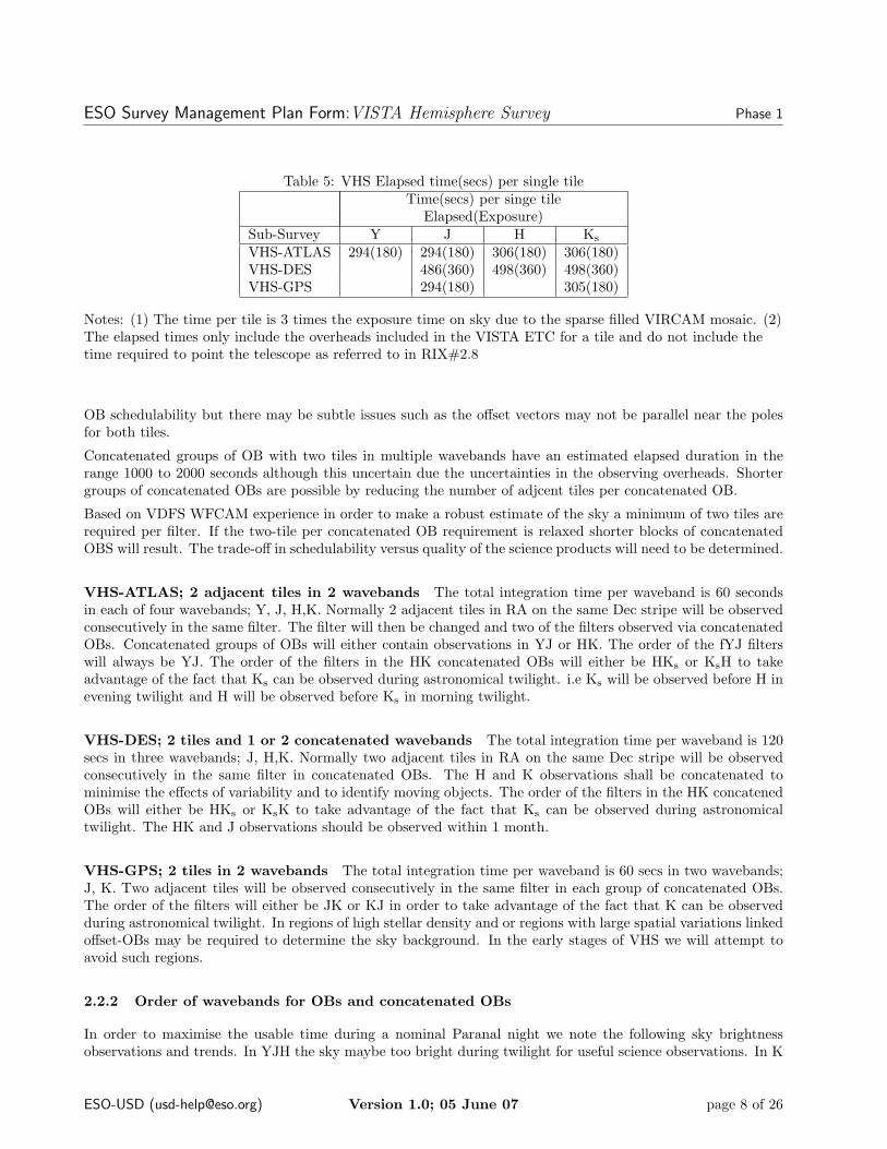
Our baseline plan is that observations use standard 6 pointing tiles which gives two observations per sky pixelwith two jitters at each pointing. This produces 4 observations per sky pixel neglecting the effect of bad pixels.The duration of a single waveband per tile OB is given in Table 5. The elapsed time per tile is in the range∼300–500 seconds (∼5–7 minutes).
All OBs or groups of concatenated OBs will have a total time less than 1 hour in duration. We require twoadjacent tiles in the same waveband to be observed consecutively in order to determine a robust sky. CurrentESO rules allow 1 tile or pointing per OB. Therefore currently each OB is a single tile in a single waveband andwe will concatenate two OBs with the same filter together. Alternatively, a double-tile could be defined withinan OB using a pointing centre and 11 offset positions. Naively this may save overheads with little impact in
ESO-USD ([email protected]) Version 1.0; 05 June 07 page 7 of 26
ESO Survey Management Plan Form:VISTA Hemisphere Survey Phase 1
Table 5: VHS Elapsed time(secs) per single tileTime(secs) per singe tile
Elapsed(Exposure)Sub-Survey Y J H Ks
VHS-ATLAS 294(180) 294(180) 306(180) 306(180)VHS-DES 486(360) 498(360) 498(360)VHS-GPS 294(180) 305(180)
Notes: (1) The time per tile is 3 times the exposure time on sky due to the sparse filled VIRCAM mosaic. (2)The elapsed times only include the overheads included in the VISTA ETC for a tile and do not include thetime required to point the telescope as referred to in RIX#2.8
OB schedulability but there may be subtle issues such as the offset vectors may not be parallel near the polesfor both tiles.
Concatenated groups of OB with two tiles in multiple wavebands have an estimated elapsed duration in therange 1000 to 2000 seconds although this uncertain due the uncertainties in the observing overheads. Shortergroups of concatenated OBs are possible by reducing the number of adjcent tiles per concatenated OB.
Based on VDFS WFCAM experience in order to make a robust estimate of the sky a minimum of two tiles arerequired per filter. If the two-tile per concatenated OB requirement is relaxed shorter blocks of concatenatedOBS will result. The trade-off in schedulability versus quality of the science products will need to be determined.
VHS-ATLAS; 2 adjacent tiles in 2 wavebands The total integration time per waveband is 60 secondsin each of four wavebands; Y, J, H,K. Normally 2 adjacent tiles in RA on the same Dec stripe will be observedconsecutively in the same filter. The filter will then be changed and two of the filters observed via concatenatedOBs. Concatenated groups of OBs will either contain observations in YJ or HK. The order of the fYJ filterswill always be YJ. The order of the filters in the HK concatenated OBs will either be HKs or KsH to takeadvantage of the fact that Ks can be observed during astronomical twilight. i.e Ks will be observed before H inevening twilight and H will be observed before Ks in morning twilight.
VHS-DES; 2 tiles and 1 or 2 concatenated wavebands The total integration time per waveband is 120secs in three wavebands; J, H,K. Normally two adjacent tiles in RA on the same Dec stripe will be observedconsecutively in the same filter in concatenated OBs. The H and K observations shall be concatenated tominimise the effects of variability and to identify moving objects. The order of the filters in the HK concatenedOBs will either be HKs or KsK to take advantage of the fact that Ks can be observed during astronomicaltwilight. The HK and J observations should be observed within 1 month.
VHS-GPS; 2 tiles in 2 wavebands The total integration time per waveband is 60 secs in two wavebands;J, K. Two adjacent tiles will be observed consecutively in the same filter in each group of concatenated OBs.The order of the filters will either be JK or KJ in order to take advantage of the fact that K can be observedduring astronomical twilight. In regions of high stellar density and or regions with large spatial variations linkedoffset-OBs may be required to determine the sky background. In the early stages of VHS we will attempt toavoid such regions.
2.2.2 Order of wavebands for OBs and concatenated OBs
In order to maximise the usable time during a nominal Paranal night we note the following sky brightnessobservations and trends. In YJH the sky maybe too bright during twilight for useful science observations. In K
ESO-USD ([email protected]) Version 1.0; 05 June 07 page 8 of 26
ESO Survey Management Plan Form:VISTA Hemisphere Survey Phase 1
science useful observations can be obtained during twilight. In YJH the sky gets darker during the night as theOH ’relaxes’. Analysis of the sky brightness trends by Riello(2007, ESO Calibration workshop) shows that themeasured K band sky brightness as observed with UKIRT WFCAM on Mauna Kea, during both evening andmorning period between nautical(12degee) and astronomical(18degree) twilight is not significantly brighter thatthe night time value. Therefore in blocks of multi-filter concatenated OBs Ks should be observed first duringevening twilight and last in the morning twilight. In principle this gains up to 30 minutes of twilight time forscience observing each night. This means that the OB order in concatenated OBs will have to be updatedperiodically for fields that are observable during twilight.
Below we consider some other filter order suggestions for each VHS component.
VHS-ATLAS YJ generally in second half of night and avoiding twilight. KH order in evening with Kobservations starting within astronomical twilight. HK order in morning twilight with K observations possibleduring astronomical twilight.
VHS-DES If all three bands as linked, the order could be KHJ in first half of night with K observationspossible during evening astronomical twilight. JHKs in last quarter of the night with K within dawn twilight.
VHS-GPS Normally we will observe tiles first in K and then the same group of tiles in J except that in finalhour of night the order should be reversed to that science observations can be carried out in K during twilight.
2.2.3 THIN and SEEING constraint
Since a prime science goal is to make the depth as uniform as possible we shall want to avoid observing inBOTH the worst permissible seeing AND in thin conditions so THIN will have a seeing limit of 1.2 whereas ingeneral CLEAR will have seeing limit of 1.4.
We would like to explore in the future the option of increasing the integration time by 50-100% in THINconditions. This would impact on the total time required. The actual impact would depend on the fraction ofobservations observed in THIN conditions and the observing overheads. This increase in time would be partiallycompensated for by a reduction in the fraction of OBs that would have to be reobserved.
2.2.4 Link between SKYBRIGHTNESS, THIN and SEEING constraints
The UKIDSS survey strategy includes the ability to increase the integration time of observations when the com-bined observed conditions would result in observations that would fail the magnitude limit science requirements.An option to increase the exposure time by 50% or 100% may be useful if we find that a significant number ofOBs tail to reach the magnitude limits required in mediocre conditions.
This is predominantly a problem in the shorter wavebands compared with K band which shows the smallestrange in sky brightness. However on particularly warm nights during the Paranal summer it may be worthconsidering increasing the K band exposures. We note that the increase in total observing time will not belinear when overheads are taken into account.
We accept that that at present ESO policies for Service Mode Observations (which will apply to VISTA ob-serving) the exposure cannot be adjusted at the telescope (Rix#2.3).
2.2.5 Very bright stars and galaxies; see also response to Rix#2.6
We are concerned about the effects of very bright stars in terms of affecting sky frames and persistence. InFigure 2 we reproduce star and galaxy counts from 2MASS (Skrutskie et al, 2006AJ....131.1163S). We may wantto avoid the brightest stars that have a surface density of 1 per 100deg2 e.g. Ks<4 in the VHS footprint during
ESO-USD ([email protected]) Version 1.0; 05 June 07 page 9 of 26

ESO Survey Management Plan Form:VISTA Hemisphere Survey Phase 1
the first period of survey operations so that we can quantify the effects caused by such stars for the pipeline anddetectors. A possible strategy would be to observe these tiles at the end of the night so that their impact onsubsequent observations is minimised. Similarly we would like to quantify the quality of the pipeline reductionfor galaxies larger than a quarter of a chip which corresponds to Ks<8 and which have a surface density of∼0.01deg−2 i.e. 1 per 60 tiles.
We request that some very bright stars and large galaxies are observed during a Science Verification phase tothat their effects are quantified. Apart from persistence effects, such observations will quantify scattering andghost effects if significant. It may be worth observing a bright star on all chips so that any chip to chip variationcan also be quantified.
2.2.6 Global strategy
In any period we will supply OBs with the same seeing requirements in adjacent stripes i.e. <1.2” or <1.4”in groups of 5 stripes on the basis that on average 10 equatorial stripes will be observed per year or 3500deg2.We will provide OBs for 7000 deg2 as a pool with half at a higher priority than the other. Half the OBs willbe in the North i.e δ > −25◦ and half in the South i.e δ < −25◦so that any wind direction constraint can beaccommodated.
2.3 PA orientation of VISTA camera
We have not decided whether observations will be at PA=0 or PA=90. A choice of PA=90 is being consideredin order to minimise the time time difference and hence observing condition variation between adjacent tilesthat require inter-tile overlap stacking due to the half-chip step size in the intra-tile mosiacing.
3 Survey data calibration needs
We anticipate that the standard VISTA calibration plan will be adequate for VHS observations. We refer to theCalibration Plan, Ref. [01], the proposed draft for the VISTA Calibration plan available at www.vista.ac.uk/vdfs/esoqc1/for further details, but summarise the main that are most relevant to VHS here:
3.1 Instrumental signature removal
Ref. [01] specifies the basic instrument calibration frames (dark frames, reset frames, dome flats and linearitycalibration, twilight flats) which will be available as part of the VISTA standard operating procedure, mainlyfrom daytime and twilight procedures.
• Dark frames: one set for each typical DIT value expected to be taken approximately weekly during daytimeand daily during the initial operations phase of VISTA.
• Dome flats: one set expected to be taken weekly during daytime, (primarily for detector health checksand logging of bad pixels).
• Linearity frames: these comprise sets of dome flats with stable illumination spanning a wide range ofdifferent exposure times. We anticipate a set of linearity frames will be taken every few months, and afterany major maintenance on the IRACE detector controllers.
• Twilight flats will be taken in several filters nightly. (There is likely to be insufficient twilight time toobtain twilight flats in all science filters every night, but a cyclic ordering should get twilight flats in allfilters every 2 nights, with priority given to those pass-bands most used recently) .
ESO-USD ([email protected]) Version 1.0; 05 June 07 page 10 of 26
ESO Survey Management Plan Form:VISTA Hemisphere Survey Phase 1
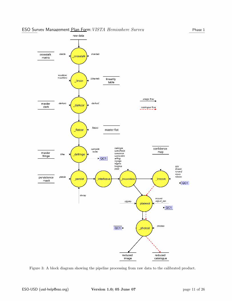
Figure 3: A block diagram showing the pipeline processing from raw data to the calibrated product.
ESO-USD ([email protected]) Version 1.0; 05 June 07 page 11 of 26
ESO Survey Management Plan Form:VISTA Hemisphere Survey Phase 1
We note here that both the VISTA dome and VIRCAM dark filter have excellent light-tightness by design (infact, VIRCAM can take dark frames in a normally-lighted lab), so daytime darks and dome flats should nothave significant leaks. This will be checked during VISTA commissioning.
3.2 Astrometric calibration
The basic astrometric procedure is a 2-stage calibration: firstly, a radial distortion correction of the form
rlin = r + k3r3 + k5r
5
is fitted, where r is image radius (in mm), k3 and k5 are distortion coefficients, rlin is a linearised radiusproportional to tan θ, where θ is angle from the pointing axis ; this form is an excellent fit to real distortion inaxisymmetric systems. The distortion parameters k3, k5 will be calculated within the VDFS pipeline on regulartime basis based on fitting to a stack of a large number of independent frames of moderately high stellar density.
For individual VIRCAM frames a catalogue of bright unsaturated stars is matched to 2MASS using the ap-proximate pointing information in the FITS headers as a start-point. The radial distortion correction is appliedto give linearised coordinates xl, yl for each measured object, then a standard 6-parameter “plate constant”solution is performed, of the form
ξ = axl + byl + c η = dxl + eyl + f
where ξ, η are standard warped tangent-plane coordinates with respect to the telescope pointing axis. Thisallows for pointing error, rotation, scale change and shear. The coefficients a . . . f are fitted with a robust fitto minimise observed-predicted residuals on a per-detector basis. The above astrometric solution will then bestored in the Multi-extension FITS headers in the ICRS system, using the ZPN notation to handle the distortion.
This procedure is very similar to that used currently for WFCAM data, which is demonstrated to give residualsover the whole field to less than 0.1 arcsec systematic and 0.1 arcsec random rms (with the latter limited by2MASS random errors at its moderate SNR ∼ 10).
While VISTA has a larger absolute distortion term, we anticipate that astrometric stability across the VISTAfocal plane is likely to be at least as good or probably better than equivalent WFCAM results, for severalreasons:
1. VIRCAM covers 3× the area of WFCAM per single pawprint, giving correspondingly more useful 2MASSstars per frame.
2. VISTA’s detectors are firmly attached to a common CTE-matched mounting plate, rather than held inZIF sockets,
3. VIRCAM’s corrective lenses are closer to the focal plane than WFCAM’s, reducing relative flexure.
4. The chromatic aberration in VIRCAM is smaller.
Additional efforts such as monitoring trends in VIRCAM-2MASS residuals over many frames and long timescalesmay be capable of reducing systematics further below the 0.1 arcsec level , but this is outside the scope of thecurrent VHS plans.
3.3 Photometric calibration
The VHS survey does not require the hourly observations of standard stars as described on page 31 in Section 5.4of the v1.4pre1 of the VDFS VIRCAM calibration plan. The VHS requirement is to photometrically calibrateVIRCAM data to 2%.
ESO-USD ([email protected]) Version 1.0; 05 June 07 page 12 of 26
ESO Survey Management Plan Form:VISTA Hemisphere Survey Phase 1
VHS photometric calibration will use 2MASS to carry out the photometric calibration of each VHS tile inYJHK using the 2MASS JHK stellar photometry following the VDFS procedures developed for the WFCAMinstrument and the UKIDSS LAS survey by Hodgkin et al(in preparation). The requirement on VDFS is tophotometrically calibrate WFCAM and VIRCAM data to 2%. Nikolaev et al. (2000) claim that the 2MASSall-sky point-source catalogue has photometry that is globally consistent to 1
For photometry, the standard instrumental signature removal of Section 3.1 corrects for dark current, non-linearity, bad pixel masking, flat-field variations does an internal gain correction to put all detectors onto auniform internal system.
After this, there are in principle three independent routes to photometric calibration:
1. Matching to 2MASS stars, with suitable colour equations.
2. Using the nightly standards (for photometric nights)
3. Global solution using matching of overlapping tiles.
The main photometric calibration will be (a) 2MASS, with method (b) used as a check and (c) applied in thelonger term when sufficient overlaps are available.
Each VIRCAM pawprint will contain over 100 useful 2MASS stars (SNR > 10 in 2MASS, and also unsaturatedin the VHS frames), corresponding to e.g. 13 <∼ J <∼ 15.
As part of the general VDFS VIRCAM calibration procedure, colour equations transforming the 2MASS systemto the VIRCAM system will be derived of the form
Jt = J2 + CJ(J2 −H2), Ht = H2 + CH(H2 −K2), . . .
where J2 etc is 2MASS magnitude, Jt is transformed to the VISTA filter system, and the colour termsCJ , CH , CK will be derived from fitting to a large number of frames and subsequently held fixed.
For routine reductions, the above colour equations with fixed coefficients give a transformed magnitude Jt,Ht,Kt
in the VISTA system for each 2MASS star.
Then due to the internal gain calibrations only a single zero-point for each pawprint is needed, e.g.
Jcal = Jins + ZPJ − eJ(X − 1),
where Jins = −2.5 log10(ADU/sec) is the raw VIRCAM instrumental magnitude, ZPJ is the zeropoint, eJ
(normally fixed) is the extinction coefficient, X is airmass and Jcal is the calibrated VIRCAM magnitude on astandard system e.g. Vega. Thus, fitting Jins − e(X − 1) vs Jt should give a line of slope 1, intercept ZPJ andsmall scatter due to 2MASS random errors and colour residuals; both of which average down in the final ZPJ .
This assumes that the 2nd order colour term from 2MASS to VIRCAM magnitude, and the colour-dependenceof extinction, are both negligible: these are generally a good approximation in the near-IR where most starshave relatively smooth spectra. Errors in the assumed extinction coefficients cancel to first order since theygive an opposite error in ZP (if a per-frame zeropoint is adopted). Also, this method is robust against isolated2MASS errors, since any single VISTA tile overlaps with a large number of distinct 2MASS stripes.
If a night is photometric, the instrument response is stable and the extinction term is correct, then all framesin the ith passband should give the same value of ZPi . Analysing trends with time or airmass can reveal non-photometric nights, long-term drift in throughput or gain (e.g. dust accumulation on the optics or IRACE gaindrift ) or errors in the assumed extinction coefficient. The VDFS CASU pipeline also computes and monitorsdetector level variations in the zeropoints as a measure of the photometricity of the observations.
3.3.1 Y band calibration
For the Y band, the situation is slightly more complex since there are no direct 2MASS measurements. (z-bandcombined with 2MASS J will be investigated as a proxy; z-band from SDSS available in some of the DES region,
ESO-USD ([email protected]) Version 1.0; 05 June 07 page 13 of 26
ESO Survey Management Plan Form:VISTA Hemisphere Survey Phase 1
and z-band data will exist soon in the SGP from the Australian Skymapper project). As a first pass, we intendto use the well-defined stellar locus to bootstrap from 2MASS J,Ks to Y band calibration as used for WFCAMcalibration within the VDFS pipeline.
The Y filter will be calibrated using 2MASS JHK stellar photometry following the procedures developed for theWFCAM instrument and the UKIDSS LAS survey by Hodgkin et al(in preparation). See also http://casu.ast.cam.ac.uk/surveys-projects/wfcam/technical/photometry. Independent checks on 2MASS based Y calibration will be carried outusing the Skymapper z band photometric survey and 2MASS J band via interpolation.
3.3.2 Illumination and geometric correction
As a final step in photometric calibration, an “illumination correction” will be applied to correct for the factthat a standard flat-fielding procedure does not lead to precise photometry, due to two effects: firstly distortionleads to varying pixel areas, and secondly stray-light forms an additive and roughly axisymmetric backgroundoffset. The illumination correction will be a position-dependent offset calculated from either stacked residualsvs 2MASS, and/or mesostepped frames across the touchstone fields.
3.4 Bad pixels
The effects of the bad pixel regions will be recorded in the VDFS confidence maps and detected sources thatare in the vicinity of spatially fixed artifacts can be flagged in the source catalogues.
3.5 Star galaxy discrimination calibration
We request that VHS depth exposures are obtained in the COSMOS field and CDFS-GEMS fields as part of thescience verification phase of VISTA. These fields have HST images that can be use to calibrate the reliabilityof star galaxy classification in VISTA.
Our backup plan is to use SDSS and other spectroscopic classifications. For instance SDSS used the COMBOsurvey classifications see: http://www.sdss.org/dr5/products/general/stargalsep.html
4 Data reduction process
We will use the VISTA Data Flow System (VDFS, Emerson et al, 2004, 2006, Irwin et al, 2004; Hambly et al,2004 ) for all aspects of data processing and archiving. The Cambridge Astronomical Survey Unit (CASU) atCambridge will be responsible for pipeline processing, and first-level calibration, and the Wide Field AstronomyUnit (WFAU) at Edinburgh will be responsible for the Science Archive with both a human and and a VOinterface with query facilities, data export capabilities and creation of higher-level products e.g. list-drivenphotometry. For a more detailed description of this system see http://www.maths.qmul.ac.uk/~jpe/vdfs/,and http://casu.ast.cam.ac.uk/ (CASU), and http://www.roe.ac.uk/~nch/wfcam/ (WFAU).
Both the VDFS pipeline and archive facilities have been designed specifically for VISTA, and have already beenscientifically verified by processing wide-field near-IR imaging from UKIRT’s WFCAM imager, at routine ratesup to 250GB/night. Versions of the pipeline have also been used to process ESO ISAAC data, and data froma wide range of optical CCD mosaic cameras. Sample from the UKIDSS project are published in Warren etal (2007MNRAS.375..213W), Dye et al (2006MNRAS.372.1227D), Lawrence et al (2006, MNRAS submitted,astro-ph/0604426) Venemans, McMahon et al (2006, MNRAS, 2007MNRAS.376L..76V, astro-ph/0612162)
We note here that VHS is a close analogue of the UKIDSS Large Area survey and the VDFS has been usedsuccessfully for this for almost two years already. There are already various papers on astro-ph that have usedUKIDSS LAS data successfuly.
ESO-USD ([email protected]) Version 1.0; 05 June 07 page 14 of 26
ESO Survey Management Plan Form:VISTA Hemisphere Survey Phase 1
The uniformity of photometric zero points across the whole survey area and the global astrometry will bechecked and verified independently by both the VDFS and VHS teams. They will be checked by the VHSteam via comparison with 2MASS and also via a comparison of photometry and astrometry for sources thatare detected in more than one tile. e.g. using the tile overlap regions
The data reduction will be using the VDFS, operated by the VDFS team, and augmented by effort from theVHS co-Is, their postdocs and graduate students, especially for Quality Control and Assurance of the VDFSproducts. We also note the considerable synergy between the science goals and the data products from VHS andVIKING survey. McMahon and Sutherland aim to collaborate on the development of automated QA proceduresfor the two surveys. In addition the VHS QA teams will work closely with the VDFS pipeline and science archivegroups.
Table 6: Responsibilities and Group LeadersName Function Affiliation CountryR. McMahon PI and OB Preparation Cambridge UKA. Lawrence Deputy/Co-PI Edinburgh UKJ. Emerson VDFS PI and OB Preparation Queen Mary, London UKCASU (VDFS) team† Pipeline processing and QC Cambridge UKWFAU (VDFS) team‡ Science Archive and QC Edinburgh UKN. Walton VO Standards Cambridge UK
VHS Survey Progress, Data Quality Control and AssuranceR. McMahon OB Preparations and Survey Progess WG leader Cambridge UKR. McMahon Data Quality WG leader Cambridge UKH-W Rix Data Quality WG leader MPIA, Heidelberg DR. Rebolo Data Quality WG leader IAC, Tenerife SF. Castander Data Quality WG leader Barcelona S
VHS Survey specific tasksT. Naylor VISTA Surveys photometry cross-calibration WG Exeter UKF. Castander DES Cordination Working Group Barcelona SF. Carrera XMM-Newton Working Group Santander SC. Bailer-Jones GAIA Working Group MPIA DJ. Emerson Photometric Calibration WG Queen Mary, London UKS. Oliver Herschel Working Group Sussex UKG. Lagache Planck Working Group IAS, Paris FH. Rottgering LOFAR and radio surveys WG Leiden NLN. Lodieu Galactic Cluster Working Group IAC SK. Romer Galaxy Cluster Working Group Sussex UK
Notes: † The CASU (VDFS) team is currently led by Irwin who is a VHS co-I. ‡ The WFAU (VDFS) team iscurrently led by Hambly who is a VHS co-I.
4.1 Pipeline processing
The VDFS pipeline is a modular design allowing alternative configurations of the processing components de-pending on the on-sky system performance of VIRCAM. Standard processing in Cambridge is on a nightly basiswith data products defined by the overall OB structure.
The VDFS pipeline at CASU will perform all the processing steps for instrumental signature removal andcatalogue generation for the VHS Tiles. The pipeline includes the following steps and is schematically shown
ESO-USD ([email protected]) Version 1.0; 05 June 07 page 15 of 26
ESO Survey Management Plan Form:VISTA Hemisphere Survey Phase 1
in Figure 3.
• instrumental signature removal – bias, non-linearity,dark, flat, fringe, cross-talk, systemic noise;
• sky background tracking and removal using all relevant OBs during a night; this may include extrahomogenisation during image stacking and mosaicing to incorporate removal of unexpected 2D systematiceffects from imperfect multi-sector operation of detectors;
• assessing and dealing with image persistence from preceding exposures if necessary (and if possible);
• combining frames if part of an observed dither sequence or tile pattern;
• producing a consistent internal photometric calibration to put observations on an approximately uniformsystem;
• image catalogue generation including astrometric, photometric, shape and Data Quality Control (DQC)information;
• final astrometric calibration based on the catalogue with an appropriate World Coordinate System (WCS)placed in all FITS headers - the default is to base this on 2MASS;
• photometric calibration for each generated catalogue using 2MASS or augmented by monitoring of suitablepre-selected standard areas covering the entire field-of-view to measure and control systematics;
• all frames and catalogues supplied with astrometric and photometric calibration information and detectedobject morphological classification embedded in FITS files;
• bad pixel handling, propagation of error arrays and effective exposure times by use of confidence maps;
• realistic errors on selected derived parameters for images and catalogues;
• nightly extinction measurements in relevant passbands;
• pipeline software version control – version used recorded in FITS header;
• processing history including calibration files recorded in FITS headers.
The pipeline processing centre hosts a data quality database that is updated daily with the data quality controlinformation for pipeline processed products. The UKIDSS WFCAM version is available at http://casu.ast.cam.ac.uk/.
Calibration library frames i.e. darks, flats are built with a significant amount of human checking. Basic qualitycontrol (e.g. rejection of frames with serious cloud, tracking/guiding failures, EMC interference, other hardwareproblems, Moon problems) will also be carried out at this stage using mainly automated procedures based onstandardised QC parameters compared with ’typical’ values. Warnings will be generated if they lie outside anapproved range (see section 6 for more details).
4.2 Science Archive
The VISTA Science Archive (VSA) at WFAU is modeled on the WFCAM Science Archive. The VSA will ingestthe metadata and catalogue outputs from pipeline processing into a relational database management system,and will then curate the FITs images and catalogues and derived products to produce enhanced database-drivenproducts.
The functions carried out by VSA will include:
• Band merging of the single waveband catalogues to provide multi-colour source lists i.e. JHKs in theVHS-DES region; JK in the VHS-GPS region and YJHKs in the VHS-ATLAS region.
ESO-USD ([email protected]) Version 1.0; 05 June 07 page 16 of 26
ESO Survey Management Plan Form:VISTA Hemisphere Survey Phase 1
• List-driven photometry to provide upper limits of objects detected in one waveband but undetected inother wavebands.
• Quality control features and metadata, as defined and agreed by the VHS team in collaboration with theVDFS team.
The VSA will have a user-friendly interface based on SQL queries; both simple and advanced interfaces areavailable, with the simple interface for ease of use while the advanced interface exposes the full relationaldatabase structure to the user enabling more complex queries and manipulation.
5 Human resources and hardware capabilities devoted to data re-duction and quality assessment
5.1 Team Members
The full list of VHS team members is given on page 1 of this document. Table 6 lists the members of the VHScollaboration who currently have specific responsibilities within the VHS collaboration. These members willwork with other members of the collaboration supplemented with effort from post-docs and graduate studentsto deliver the agreed VHS science products to ESO.
The VHS team is large but has a few nodes that have a critical mass in terms of experience and number ofco-Is. Some specific groups and group leaders are listed below:
• Barcelona(ICE, IFAE, CIEMAT); Castander
• Cambridge(IOA); McMahon
• Edinburgh (IFA); Lawrence
• Heidelberg(MPIA); Rix
• London (QMUL); Emerson
• Tenerife(IAC); Rebolo
The six named individuals are members of the VHS Management Board.
McMahon, Lawrence and Emerson are co-I’s of the VDFS project. A number of the VHS co-I’s were members ofthe team who worked on the early phases of the SDSS. e.g. Castander, Loveday, Nichol. They have considerableexperience in wide field survey image and catalogue quality assurance. The VHS team also consists of membersof the ESO community who are members of the UKIDSS consortium who have have involved in the UKIDSSLAS survey. The VHS team also include the PIs of four other VISTA public surveys (Jarvis, Cioni, Lucas,Sutherland) and this will facilitate the exchange of quality control and assurance best practice between theprojects.
A number of major institutes have multiple co-I and thus will have the local critical mass. These co-I’s will leadindependent but coordinated Quality Control and Assurance working groups i.e. MPIA, Heidelberg, Rix et al;Barcelona, Castander et al; Rebolo et al, IAC; McMahon et al, Cambridge. Data quality control and assurancewill be a distributed task across the consortium within four working groups working semi-independently withsome tasks replicated. It will be coordinated by the four group leaders who will meet via Telecon with othersleading QA taks on a monthly basis when the data starts to flow. Other members of the collaboration will workwith these teams.
Experience shows that the a full data scientific validation is only possible when people start trying to do sciencewith the data. Thus in addition to the quality assurance working groups we will also have a number of Scientific
ESO-USD ([email protected]) Version 1.0; 05 June 07 page 17 of 26
ESO Survey Management Plan Form:VISTA Hemisphere Survey Phase 1
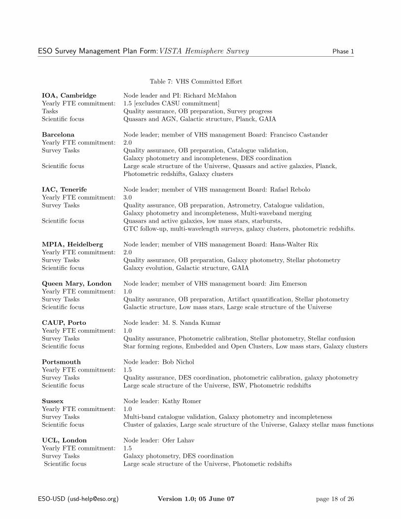
Table 7: VHS Committed Effort
IOA, Cambridge Node leader and PI: Richard McMahonYearly FTE commitment: 1.5 [excludes CASU commitment]Tasks Quality assurance, OB preparation, Survey progressScientific focus Quasars and AGN, Galactic structure, Planck, GAIA
Barcelona Node leader; member of VHS management Board: Francisco CastanderYearly FTE commitment: 2.0Survey Tasks Quality assurance, OB preparation, Catalogue validation,
Galaxy photometry and incompleteness, DES coordinationScientific focus Large scale structure of the Universe, Quasars and active galaxies, Planck,
Photometric redshifts, Galaxy clusters
IAC, Tenerife Node leader; member of VHS management Board: Rafael ReboloYearly FTE commitment: 3.0Survey Tasks Quality assurance, OB preparation, Astrometry, Catalogue validation,
Galaxy photometry and incompleteness, Multi-waveband mergingScientific focus Quasars and active galaxies, low mass stars, starbursts,
GTC follow-up, multi-wavelength surveys, galaxy clusters, photometric redshifts.
MPIA, Heidelberg Node leader; member of VHS management Board: Hans-Walter RixYearly FTE commitment: 2.0Survey Tasks Quality assurance, OB preparation, Galaxy photometry, Stellar photometryScientific focus Galaxy evolution, Galactic structure, GAIA
Queen Mary, London Node leader; member of VHS management board: Jim EmersonYearly FTE commitment: 1.0Survey Tasks Quality assurance, OB preparation, Artifact quantification, Stellar photometryScientific focus Galactic structure, Low mass stars, Large scale structure of the Universe
CAUP, Porto Node leader: M. S. Nanda KumarYearly FTE commitment: 1.0Survey Tasks Quality assurance, Photometric calibration, Stellar photometry, Stellar confusionScientific focus Star forming regions, Embedded and Open Clusters, Low mass stars, Galaxy clusters
Portsmouth Node leader: Bob NicholYearly FTE commitment: 1.5Survey Tasks Quality assurance, DES coordination, photometric calibration, galaxy photometryScientific focus Large scale structure of the Universe, ISW, Photometric redshifts
Sussex Node leader: Kathy RomerYearly FTE commitment: 1.0Survey Tasks Multi-band catalogue validation, Galaxy photometry and incompletenessScientific focus Cluster of galaxies, Large scale structure of the Universe, Galaxy stellar mass functions
UCL, London Node leader: Ofer LahavYearly FTE commitment: 1.5Survey Tasks Galaxy photometry, DES coordinationScientific focus Large scale structure of the Universe, Photometic redshifts
ESO-USD ([email protected]) Version 1.0; 05 June 07 page 18 of 26
ESO Survey Management Plan Form:VISTA Hemisphere Survey Phase 1
Working groups (following the themes of the goals listed in the science objectives). Table 6 lists the currentset of exemplary groups. Any data quality problems found by these teams will be passed to one or more of thequality control working groups as required.
5.1.1 VHS committed effort
In Table 7 we list the effort that has been committed by the members of he VHS to the project. Only nodes thathave committed 1.0 or more FTEs are listed. OB preparation will be cordinated by McMahon and Emersonwith effort also from Heidelberg, Barcelona and Tenerife. The total effort commited to the task is 1.0 FTE peryear.
5.2 VDFS human resources and hardware capabilities
The VDFS UK pipeline will be used to process all data taken on VISTA. Based on 2 years of experience atrunning the WFCAM processing pipeline, CASU have estimated their human resource requirements to carry outthe tasks outlined above in section 4.1 as 3 FTE. This includes normal processing, quality control, reprocessingafter major bug fixes and/or enhancements, system maintenance and upgrades, and liaison with major users.
Hardware CPU requirements for the Cambridge processing pipeline are specified to have an overcapacity of afactor of at least 3 (to allow for the inevitable variations of data flow rates and reprocessing requirements).Data storage will be purchased as required and all raw and processed files will be stored using lossless Rice tilecompression to save a factor of 4 in hardware requirements.
Manpower provision at the VDFS Edinburgh science archive centre currently stands at 2.0 FTE dedicated oper-ations staff and around 1.0FTE of astronomer-scientist management, oversight and systems support. Hardwareprovision for storage of pipeline-processed science product files, database server catalogue storage and associatedweb servers and other infrastructure is currently funded, via a rolling grant, to 2010 and is renewed every twoto three years.
6 Data quality assessment process
The assessment of data quality is is a 3-stage process: a quick assessment is performed at Paranal, then followingVDFS pipeline processing a second stage (QC-I) performed by VDFS, and the final stage(QC-II) before generaldata release is the responsibility of the VHS team. These stages are outlined in more detail below.
6.1 VHS Data quality assessment and control process
The VHS PI will be the primary point of contact between the VHS collaboration and the overall VDFS project.In addition VHS will identify individuals who will be the primary day to day point of contact at each of thetwo main components of the VDFS; (i) the VDFS-Pipeline at CASU, Cambridge and (ii) the VDFS ScienceArchive at WFAU, Edinburgh. The VHS team will define and agree in consultation with the VDFS team(s),QC criteria that can be applied to the VDFS VISTA dataproducts in advance of preparing data releases to theESO SAF.
The QC criteria and thresholds will be communicated to the VDFS via the VHS consortium primary point ofcontact. In practice the QC work may involve one of more individuals from the VHS consortium working closelyin-situ for a period with one or both of the two VDFS groups.
Within the VDFS project considerable effort has gone into automated QC parameter generation in the pipelinedesign, (see the Data Reduction Library Design v1.6 available at http://www.vista.ac.uk/vdfs/esoqc1/) forfurther information). The most basic version of the QC process occurs in near-time on Paranal, while more
ESO-USD ([email protected]) Version 1.0; 05 June 07 page 19 of 26
ESO Survey Management Plan Form:VISTA Hemisphere Survey Phase 1
sophisticated versions will be run in Garching and later in Cambridge. All of the Cambridge pipeline QC infor-mation will be available to VHS Quality Assurance teams via a QC database in Cambridge (for an example seehttp://casu.ast.cam.ac.uk/surveys-projects/wfcam/data-processing/) and is also recorded in the data productFITS headers.
The VHS quality control process will include the requirement to identify obvious datasets where the pipeline hasunder performed in some clear manner and feeding information back to the CASU group so that an investigationof what went wrong can be put in place. If the pipeline is clearly at fault then early reprocessing with modifiedpipeline components will take place.
The quality control process will also consist of identifying datasets where the observations were carried outincorrectly, ie. appropriate calibration files were not available, or in bad conditions. Such datasets that cannotbe fixed by altering the pipeline and may need to be reobserved with appropriate changes to the observingstrategy. Note that the catalogue generated QC information will help to pick out these cases but some level ofvisual inspection will also be planned for. The VDFS WFCAM pipeline DQC and survey progress graphicalinterface is available here: http://casu.ast.cam.ac.uk/survey-progress/wfcam/.
The Archive quality control process itself consists of a data modification script coded up manually by the VDFSscience archive staff based on the QC criteria specified by the EPS consortium. Quality Control issues currentlyimplemented in the WFCAM Science Archive can be viewed at this URL: http://surveys.roe.ac.uk/wsa/www/gloss d.html#lasdetection deprecated.Example QC plots and further information can be found in Dye et al., MNRAS, 372, 1227 (2006) and Warrenet al., 2007MNRAS.375..213W)
6.2 VDFS quality control
In the VDFS pipeline, considerable effort has gone into the design of automated QC parameters which aregenerated automatically during the reductions and compared with typical ranges. All of the CASU pipeline QCinformation will be made available to the VHS team via a web-based QC interface (for an example, see Ref. [05]) and these QC parameters are also recorded in the FITS headers.
A complete list of QC parameters are available in Ref. [02] Appendix A , while some examples include:
• Pointing differences between blind telescope pointing and final calibrated WCS.
• Mean sky level and rms noise.
• Number of objects classified as “noise”.
• Saturation level (from bright stars)
• Mean FWHM and ellipticity for objects classified as “stellar”.
• Aperture correction (fraction of stellar flux outside 2 arcsec).
• Photometric zeropoint from 2MASS
• Photometric zeropoint from nightly standards
• Stellar magnitude limit (computed from the above).
In order to maxmise the legacy value of the VHS survey the VHS team plans to produce an online ExplanatorySupplement modeled on the 2MASS Explanatory Supplement (http://www.ipac.caltech.edu/2mass/releases/allsky/doc/explsup.html)
6.3 VHS team quality control
Additional tests that may be done at both the post-pipeline and post-archive stage by the VHS QC team,include the following:
ESO-USD ([email protected]) Version 1.0; 05 June 07 page 20 of 26
ESO Survey Management Plan Form:VISTA Hemisphere Survey Phase 1
• Low resolution tile background images binned at 32x32 pixels to produce 406x512 pixels images whichcan be eyeballed initially and used to develop and train objective machine based techniques with possiblehuman intervention as required.
• Tile level dot plots that show the spatial distributions of stars and galaxies and noise objects.
• Tile level spatial distributions of matched and unmatched objects from the multi-colour band merging.
• Colour counts and median colours as a function of magnitude for each tile and compared with templateresults.
• Additional checks of QC parameters generated by the pipeline, to look for low-level effects or trends whichmay not trigger the automated warnings.
• Inspection of colour-colour and colour-magnitude diagrams at a single Tile level In general stars andgalaxies lie on distinct sequences in near-IR colour-colour space, with most stars forming a relativelytight locus, so inspection of these plots plus morphological classification forms a powerful check for manysystematic errors (see Ref [06] for examples).
• Masking of defects: Localised image problems are usually apparent by inspection of dot-plots, especiallyfor objects of unusual colours. Localised problems creating significant numbers of spurious images (suchas diffraction spikes, aircraft or satellite trails, bright-star ghosts etc) are readily apparent.Based on early experience, we will create an automated masking and flagging around bright stars, i.e. flaga magnitude-dependent radius around each bright star.
• Overlap matching. The VHS conservative tiling strategy will provide significant edge overlaps ∼ 2 arcminwide at the North and South edges of each tile, containing > 100 objects per overlap. Thus, comparisonof image parameters for objects duplicated in the overlap regions will provide a strong check of mostsystematic errors (with the exception of centre-to-edge systematics which will be investigated via thestacking of residuals from mean properties). Larger samples are available from the ’wings’ 5.5 arcminwide with full exposure in one tile and half in the other.
During the early stages of the public survey all images and catalogue products will be visually verified bythe VHS team. The goal is develop and train machine learning based techniques that require only humanintervention in the case of 1-2% of tiles.
The VHS quality assurance will be divided up into a range of tasks that will then be managed by the QA team.Some specific tasks that are planned in addition to the list above are:
1. Independent source catalogue generation
2. Source catalogue validation
3. Astrometry
4. Star-galaxy separation
5. Photometric calibration
6. Stellar photometry
7. Stellar confusion
8. Stellar incompleteness
9. Galaxy photometry
10. Galaxy incompletness
11. Multi-waveband merging
12. Artifact characterisation and quantification
ESO-USD ([email protected]) Version 1.0; 05 June 07 page 21 of 26
ESO Survey Management Plan Form:VISTA Hemisphere Survey Phase 1
7 Data product and VO compliance:
The VHS products that will be delivered to the ESO SAF are listed below. All products will be FITS imagesor tables with metadata contained within the FITs headers to fufil the ESO VO requirements as defined inhttp://www.eso.org/observing/ps/VOS-RRD.pdf. The VDFS will be used able to deliver flat FITS images andcatalogues on a tile basis to the ESO Science Archive Facility as follows:
(a) Tile based survey quality-controlled pipeline processed products: instrumentally corrected stacked sci-ence frames along with their associated single-passband catalogue detection lists, all photometrically andastrometrically calibrated from 2MASS.
(b) The catalogue products are defined in the VDFS document VDF-SPE-IOA-00009-0001v4(Irwin, 2007)and is available at this URL: http://www.ast.cam.ac.uk/ rgm/vhs/smp/WFCAM-catalogues-v4p0.pdf.The extraction parameters were initially developed as part of the science requirements analysis by the UKcommunity for the VISTA pipeline and the UKIDSS surveys. The PI and many other members of theVHS team were involved in both these processes. In the case of the UKIDSS surveys the ESO communityhas also been involved.
The current set of parameters will be reviewed during the period when VHS is being carried out, to ensurethat the VHS parameter set are consistent with the parameter sets for VST ATLAS and DES.
(c) Confidence maps, dark frames and flat fields used in the production of (a).
(d) Tile based associated source catalogues linking the parameters of individual objects across all of theobserved filter bands.
(e) Aperture matched photometry and aperture based upper limits for sources detected in (a).
All available metadata will be included in the FITS headers. The VHS data will be delivered from the VSA tothe ESO Science Archive via the Internet.
8 Timeline delivery of data products to the ESO archive:
Raw VISTA data is normally expected to arrive in the UK roughly 2-3 weeks days after the observationsare taken. The turnaround time for ingesting and verifying the raw data is expected to be normally anotherworking week assuming no significant problems. CASU estimate that when a steady state is reached for thedata processing normally data will have been pipeline processed and QC checked by CASU within 3-4 workingweeks of successful data ingest. Data will then be available for VHS quality assurance and transfer to the VistaScience Archive in Edinburgh with secure data access provided to the VHS quality assurance teams.
Normally during the steady state, VHS expects that it will deliver the agreed survey data products using theVDFS to the ESO Science Archive before the end of the semester following the one in which the raw data weredelivered to CASU.
Based on recent experience from the SDSS and UKIDSS projects we anticipate that a longer delivery periodwill be required for at least the first full semesters and possibly also for the second full semester. We thereforewish to make provision for a more extended quality control and analysis period by the VDFS and VHS teamsduring the first year of public survey operations and to allow for a VDFS reprocessing phase with improvedsoftware parameters to correct problems discovered in the first-look analyses of the data from the first period ofobservations. We also request the provision of survey science verifiation phase where a series observations canbe carried out so that observing strategy can be optimised.
We estimate that the data products from the first period of VHS observation data could be delivered to ESOnot more than one year later than the end of the first full period i.e. by the end of the third observing period.
ESO-USD ([email protected]) Version 1.0; 05 June 07 page 22 of 26
ESO Survey Management Plan Form:VISTA Hemisphere Survey Phase 1
There would then be a ’catch up’ phase with a goal of delivering the 2nd period of observations during the 4thperiod and the 3rd period of observations by the end of the 4th period and thereafter we would follow the oneperiod for data delivery model.
Thus for example, assuming VHS observations start in period 80, the delivery of period 80 data would be bythe end of period 82. Period 81 data would be delivered sometime during period 83 and period 82 by the endof period of period 83. This will clearly be somewhat in advance of a presumed 2-year review which wouldnominally be carried out during period 84. If required we could release a subset of the first period of dataearlier in the form of an ’Early Data Release’ which is a model which has been used by successfully by 2MASS,SDSS and UKIDSS. This would consist of a small representative set of data. For example 2MASS released asingle night of data from the night of 1997 November 16 a year later on 1998 Dec 8. They then had their firstmajor release of data covering data data between 1997 June and 1998 January in 1999 May. The content anddelivery plan for the VHS Early Data Release could be timed so that feedback from this data could be used forone of the the 6 monthly progress reviews.
9 References
[01] P. Bunclark and S. Hodgkin. “VISTA Infrared Camera Calibration Plan”, VIS-SPE-IOA-20000-0002, v1.4,2006/11/13.
[02] J. Lewis, P. Bunclark, S. Hodgkin., “VISTA Data Reduction Library Design”, VIS-SPE-IOA-20000-0010,v1.6, 2006/12/20.
[03] ”VISTA Data Flow System: Status” Jim Emerson, Mike Irwin, Nigel Hambly in Observatory Operations:Strategies, Processes, and Systems, edited by David R. Silva, Rodger E. Doxsey, Proc. of SPIE Vol. 6270, 30,2006
”VISTA Data Flow System: Overview” Jim Emerson, Mike Irwin, Jim Lewis, Simon Hodgkin, Dafydd Evans,Peter Bunclark, Richard McMahon, Nigel Hambly, Robert Mann, Ian Bond, Eckhard Sutorius, Michael Read,Peredur Williams, Andrew Lawrence, Malcolm Stewart in Observatory Operations: Strategies, Processes, andSystems, eds David R. Silva, Rodger E. Doxsey,Proc. of SPIE Vol. 5493, 401, 2004
VISTA data flow system: pipeline processing for WFCAM and VISTA, Irwin, Bunclark, Evans, Hodgkin, Lewis,McMahon, Emerson, Beard, Stewart, in Optimizing Scientific Return for Astronomy through Information Tech-nologies, eds Quinn & Bridger, Proc of SPIE, 5493, 411, 2004VISTA data flow system: survey access and curation: the WFCAM science archive, Hambly, Mann, Bond,Sutorius, Read, Williams, Lawrence, Emerson, in Optimizing Scientific Return for Astronomy through Infor-mation Technologies, eds Quinn & Bridger, Proc of SPIE, 5493, 423, 2004
[04] http://www.vista.ac.uk/vdfs/esoqc1/
[05] http://casu.ast.cam.ac.uk/surveys-projects/wfcam/data-processing/ ,
[06] Dye, S. et al, 2006, MNRAS, 372, 1227.
Appendix 1: Spreadsheet tables
ESO-USD ([email protected]) Version 1.0; 05 June 07 page 23 of 26
ESO Survey Management Plan Form:VISTA Hemisphere Survey Phase 1
VHS_ATLAS SMP_VHS_obs_spreadsheet_v3p0.xls
Z Y J H KsTime & depth on sky in coadded TilesDepth (Vega) required 20.3 19.9 19.0 17.9Depth(AB) required 20.9 20.9 20.3 19.8Sigma required 5.0 5.0 5.0 5.0AssumptionsSED assumed in ETC BB10000 BB10000 BB10000 BB10000Aperture assumed in ETC - arcsec 2.0 2.0 2.0 2.0In band sky brightness assumed - Vega mag/arcsec 17.2 16.0 14.1 13.0Airmass assumed in ETC 1.2 1.2 1.2 1.2In band on-chip image size assumed - arcsec 1.2 1.2 1.2 1.2Extra extinction assumed 0.00 0.00 0.00 0.00Detector Integration Time (DIT) sec 15 15 7.5 7.5N.B. the DIT assumed will affect the number of seconds to reach a specified depth, because it affects the amount of read noise.
Time required per object sec 60 60 60 60Area required sq. deg 5000 5000 5000 5000Tiles required to cover area(s) 3484 3484 3484 3484Effective useful sq deg/tile 1.435 1.435 1.435 1.435Priorities of different areas? yes yes yes yes
Single Tile StrategyParameters setDIT already assumed above 15 15 7.5 7.5Exposure coadds (Ndit) # 1 1 2 2Exposure loops (Nexp) # 1 1 1 1Microsteps (Nmicro) # steps <3 arcsec 1 1 1 1Jitters (Njitter) # steps odd # of 0.5 pixels < 30 arcsec 2 2 2 2Pawprints in tile (Npaw) 6 6 6 6Repeat tile in same OB how many times? 1 1 1 1Multiple filters in same OB? If so which?Mutiple tile positions in same OB? If so number?Resulting valuesTotal Exposure sec/tile 180 180 180 180Total Elapsed sec/tile 293.7 293.7 305.7 305.7Total Elapsed hr/tile 0.08 0.08 0.08 0.08Observing efficiency %/tile 61.3 61.3 58.9 58.9Time per object for s-to-n -single OB 60 60 60 60Signal to noise (at depth required in row 3) - single OB 5 5 5 5Depth[Vega] (to 5 sigma) - single OB 20.3 19.9 19.0 17.9
Multiple Tile Strategy# of Tiles per filter for S/N 1 1 1 1Time links between OBs in same filter on a Tile? no no no noPriorities between OBs in same filter on a Tile? no no no noTime links between OBs on a Tile in different filters? yes yes yes yesPriorities between OBs on a Tile in different filters? yes yes yes yesTime links between Tiles by position? yes yes yes yesPriorities between Tiles by position? yes yes yes yes
Total Elapsed Hours per filter including ETC overheads 284.3 284.3 295.9 295.9Total Elapses Hours per filter with no overheads 174.2 174.2 174.2 174.2Effiicency for each waveband 61.3 61.3 58.9 58.9
Total Elapsed time 876.0Total time with no overheads 522.6Average Observing Efficiency 59.7
Figure 4: VHS-ATLAS observation requirements
ESO-USD ([email protected]) Version 1.0; 05 June 07 page 24 of 26
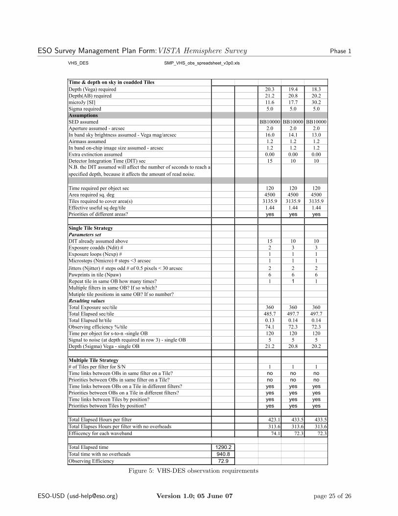
ESO Survey Management Plan Form:VISTA Hemisphere Survey Phase 1
VHS_DES SMP_VHS_obs_spreadsheet_v3p0.xls
Time & depth on sky in coadded TilesDepth (Vega) required 20.3 19.4 18.3Depth(AB) required 21.2 20.8 20.2microJy [SI] 11.6 17.7 30.2Sigma required 5.0 5.0 5.0AssumptionsSED assumed BB10000 BB10000 BB10000Aperture assumed - arcsec 2.0 2.0 2.0In band sky brightness assumed - Vega mag/arcsec 16.0 14.1 13.0Airmass assumed 1.2 1.2 1.2In band on-chip image size assumed - arcsec 1.2 1.2 1.2Extra extinction assumed 0.00 0.00 0.00Detector Integration Time (DIT) sec 15 10 10N.B. the DIT assumed will affect the number of seconds to reach a specified depth, because it affects the amount of read noise.
Time required per object sec 120 120 120Area required sq. deg 4500 4500 4500Tiles required to cover area(s) 3135.9 3135.9 3135.9Effective useful sq deg/tile 1.44 1.44 1.44Priorities of different areas? yes yes yes
Single Tile StrategyParameters setDIT already assumed above 15 10 10Exposure coadds (Ndit) # 2 3 3Exposure loops (Nexp) # 1 1 1Microsteps (Nmicro) # steps <3 arcsec 1 1 1Jitters (Njitter) # steps odd # of 0.5 pixels < 30 arcsec 2 2 2Pawprints in tile (Npaw) 6 6 6Repeat tile in same OB how many times? 1 1 1Multiple filters in same OB? If so which?Mutiple tile positions in same OB? If so number?Resulting valuesTotal Exposure sec/tile 360 360 360Total Elapsed sec/tile 485.7 497.7 497.7Total Elapsed hr/tile 0.13 0.14 0.14Observing efficiency %/tile 74.1 72.3 72.3Time per object for s-to-n -single OB 120 120 120Signal to noise (at depth required in row 3) - single OB 5 5 5Depth (5sigma) Vega - single OB 21.2 20.8 20.2
Multiple Tile Strategy# of Tiles per filter for S/N 1 1 1Time links between OBs in same filter on a Tile? no no noPriorities between OBs in same filter on a Tile? no no noTime links between OBs on a Tile in different filters? yes yes yesPriorities between OBs on a Tile in different filters? yes yes yesTime links between Tiles by position? yes yes yesPriorities between Tiles by position? yes yes yes
Total Elapsed Hours per filter 423.1 433.5 433.5Total Elapses Hours per filter with no overheads 313.6 313.6 313.6Effiicency for each waveband 74.1 72.3 72.3
Total Elapsed time 1290.2Total time with no overheads 940.8Observing Efficiency 72.9
Figure 5: VHS-DES observation requirements
ESO-USD ([email protected]) Version 1.0; 05 June 07 page 25 of 26
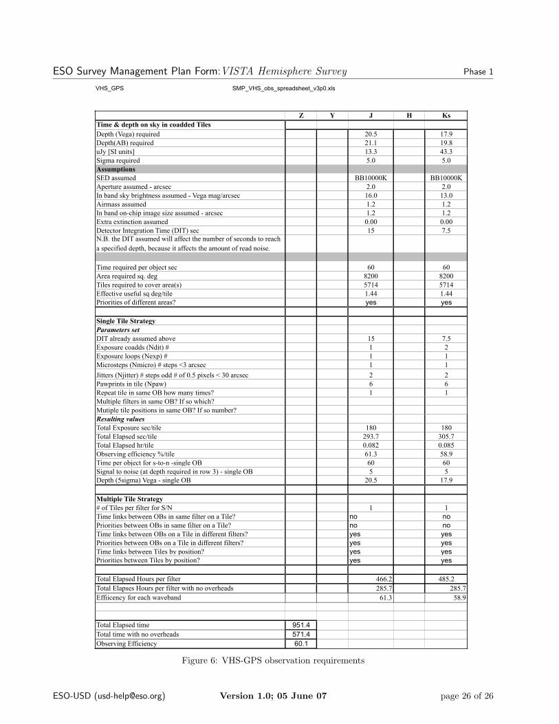
ESO Survey Management Plan Form:VISTA Hemisphere Survey Phase 1
VHS_GPS SMP_VHS_obs_spreadsheet_v3p0.xls
Z Y J H KsTime & depth on sky in coadded TilesDepth (Vega) required 20.5 17.9Depth(AB) required 21.1 19.8uJy [SI units] 13.3 43.3Sigma required 5.0 5.0AssumptionsSED assumed BB10000K BB10000KAperture assumed - arcsec 2.0 2.0In band sky brightness assumed - Vega mag/arcsec 16.0 13.0Airmass assumed 1.2 1.2In band on-chip image size assumed - arcsec 1.2 1.2Extra extinction assumed 0.00 0.00Detector Integration Time (DIT) sec 15 7.5N.B. the DIT assumed will affect the number of seconds to reach a specified depth, because it affects the amount of read noise.
Time required per object sec 60 60Area required sq. deg 8200 8200Tiles required to cover area(s) 5714 5714Effective useful sq deg/tile 1.44 1.44Priorities of different areas? yes yes
Single Tile StrategyParameters setDIT already assumed above 15 7.5Exposure coadds (Ndit) # 1 2Exposure loops (Nexp) # 1 1Microsteps (Nmicro) # steps <3 arcsec 1 1Jitters (Njitter) # steps odd # of 0.5 pixels < 30 arcsec 2 2Pawprints in tile (Npaw) 6 6Repeat tile in same OB how many times? 1 1Multiple filters in same OB? If so which?Mutiple tile positions in same OB? If so number?Resulting valuesTotal Exposure sec/tile 180 180Total Elapsed sec/tile 293.7 305.7Total Elapsed hr/tile 0.082 0.085Observing efficiency %/tile 61.3 58.9Time per object for s-to-n -single OB 60 60Signal to noise (at depth required in row 3) - single OB 5 5Depth (5sigma) Vega - single OB 20.5 17.9
Multiple Tile Strategy# of Tiles per filter for S/N 1 1Time links between OBs in same filter on a Tile? no noPriorities between OBs in same filter on a Tile? no noTime links between OBs on a Tile in different filters? yes yesPriorities between OBs on a Tile in different filters? yes yesTime links between Tiles by position? yes yesPriorities between Tiles by position? yes yes
Total Elapsed Hours per filter 466.2 485.2Total Elapses Hours per filter with no overheads 285.7 285.7Effiicency for each waveband 61.3 58.9
Total Elapsed time 951.4Total time with no overheads 571.4Observing Efficiency 60.1
Figure 6: VHS-GPS observation requirements
ESO-USD ([email protected]) Version 1.0; 05 June 07 page 26 of 26