1

ViSta-CITA “Classical Item & Test Analysis with ViSta” Rubén Ledesma & J. Gabriel Molina

This report describes ViSta-CITA, a computer application for psychometric item and test analysis designed to work as plugin in the ViSta statistical program. Vista-CITA provides a sample of computerized tools which support analysis of item and test scores based on general statistics usual in psychometric analysis as well as some procedures associated to Classical Test Theory (CTT1). As it is standard in the ViSta system, two ways of visualizing the results are available to the user for each one of the analysis procedures considered in ViSta-CITA: (1) a listing or report of numerical information about the analysis model applied, that is, the way many classical programs offer the analysis results; (2) a graphical visualization of the results of the analysis. The latter is raised through spreadplots (Young, Valero, Faldowsky & Bann, 2000), a ViSta graphical concept consisting of linked list and plot windows that shows different aspects of the application of an analysis procedure. ViSta-CITA may be also used to generate new data variables like different kinds of test scores for the subjects.

CONTENTS:

1. USING ViSta-CITA

1.1. Preparing Data for Analysis

1.2. Analysis Options

1.3. Obtaining Reports

1.4. Obtaining Visualizations

1.5. Creating Data

2. EXAMPLE

2.1. Analysis based on Cronbach’s Alpha (Alpha Model)

2.1.1. Report for the Alpha Model

2.1.2. Visualization for the Alpha Model

2.2. Split-Half Analysis (Split-Half Model)

2.2.1. Report for the Split-Half Model

2.2.2. Visualization for the Split-Half Model

2.3. Analysis based on Principal Component Analysis (PCA Model)

2.3.1. Report for the Theta Model

2.3.2. Visualization for the Theta model

3. ALGORITHMS

4. REFERENCES

1 For a compressive exposition of CTT consult, for example, Gulliksen (1950), or Lord and Novick (1968).

2

1. USING ViSta CITA

1.1. Preparing Data for Analysis

ViSta-CITA analyzes multivariate data containing more than 3 numeric variables (items). Each cell

represents the score (or just the response) of a subject (row) to an item (column). In order to analyze a

dataset with Vista-CITA, it must be run Vista and loaded into the system the file with the dataset to be

analyzed. There are three options for this task:

(1) Existing ViSta data files can be loaded into ViSta using the Open Data menu item.

(2) New data may be entered through the ViSta data editor (New Datasheet menu item).

(3) Text or excel files can be imported using the ViSta Import Data item.

The data must be numeric and complete (no empty cells). If missing data exists in your dataset,

you could use the ViSta Impute Missing Data command. Since the user can select a subset of variables

before proceeding with the analysis, the dataset may contain any other kind of variables than item

responses/scores.

1.2. Analysis Options

You can perform ViSta-CITA psychometric analysis by selecting the Item-Test Analysis item from the

Analysis menu. Then, you will see a dialog box with the following analysis options: a) Internal consistency

analysis based on Cronbach’s alpha, b) Split-half reliability analysis, and c) Analysis based on Theta, a

coefficient derived from PCA (Principal Component Analysis). Selecting one of these methods will

produce a model of your data. You can look at the model of your data in ViSta by asking for a report or a

visualization of the model.

1.3. Obtaining Reports

A report of your model produces a listing of numeric information about the analysis model applied to your

data. After applying an analysis model in ViSta (Analysis menu), you can get a report of the model by

selecting the Report Model item from the Model menu (or, also, by clicking on the report button on the

WorkMap’s toolbar, by clicking on the report icon attached to the model icon, or by typing ‘(report-model)’

in the Vista Listener. After choosing this command, a report dialog box will show some options to the

program user. Note that the options in this dialog window depend on the analysis model that has been

previously applied. A basic report may be obtained by simple clicking OK. Longer results may be obtained

by selecting the options shown in the dialog box.

1.4. Obtaining Visualizations

When you visualize your analysis model in Vista, the program purpose is you can “see what your model

seems to say”. You can obtain a visualization for your model by selecting the Visualize Model item from

the Model menu. Then, a spreadplot will be computed and shown. Spreadplots are a ViSta graphical

concept consisting of linked list and plot windows that shows different aspects of the application of an

3

analysis model. Three different spreadplots have been implemented in ViSta-CITA, one for each of the

three analysis models considered in this module at the moment.

1.5. Creating Data

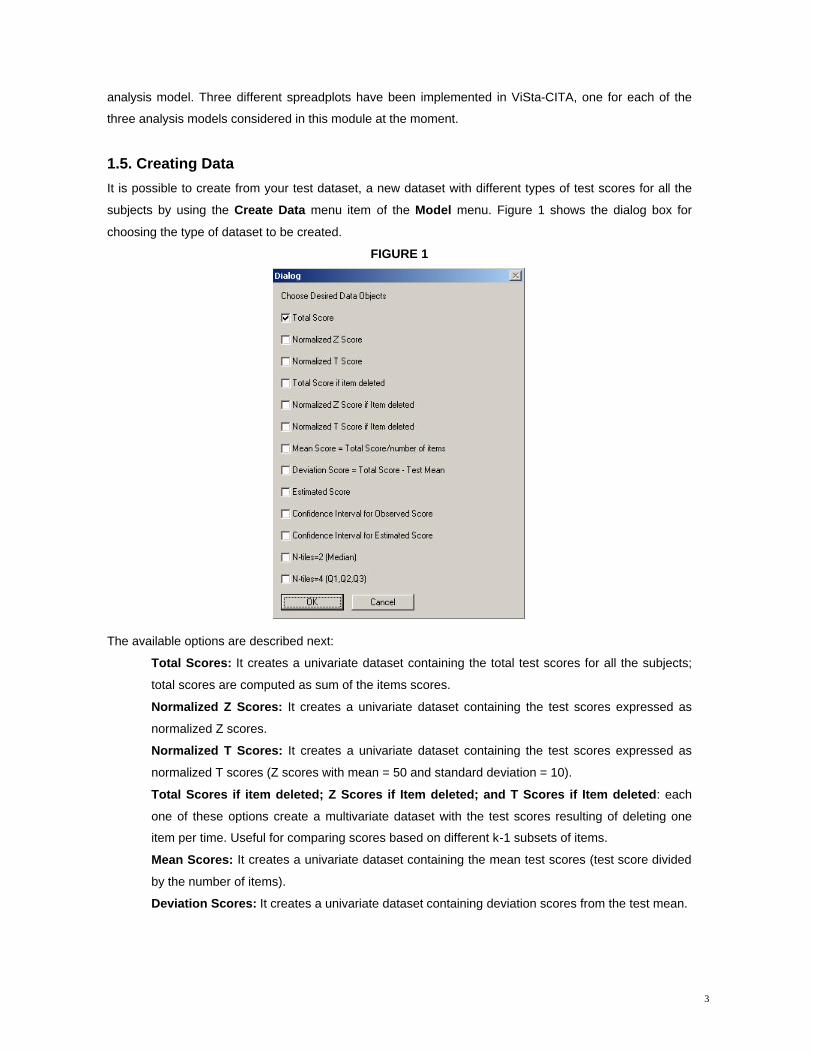
It is possible to create from your test dataset, a new dataset with different types of test scores for all the

subjects by using the Create Data menu item of the Model menu. Figure 1 shows the dialog box for

choosing the type of dataset to be created.

FIGURE 1

The available options are described next:

Total Scores: It creates a univariate dataset containing the total test scores for all the subjects;

total scores are computed as sum of the items scores.

Normalized Z Scores: It creates a univariate dataset containing the test scores expressed as

normalized Z scores.

Normalized T Scores: It creates a univariate dataset containing the test scores expressed as

normalized T scores (Z scores with mean = 50 and standard deviation = 10).

Total Scores if item deleted; Z Scores if Item deleted; and T Scores if Item deleted: each

one of these options create a multivariate dataset with the test scores resulting of deleting one

item per time. Useful for comparing scores based on different k-1 subsets of items.

Mean Scores: It creates a univariate dataset containing the mean test scores (test score divided

by the number of items).

Deviation Scores: It creates a univariate dataset containing deviation scores from the test mean.

4

Estimated Scores: It creates a univariate dataset containing estimated scores given the current

test mean, SD and Alpha reliability coefficient (by default). You can modify these parameters by

using the dialog box that appears when this option is selected.

Confidence Interval for Observed Scores (Total Scores): it creates a multivariate dataset with

confidence interval (a=0.05, by default) for the observed test scores (total scores)given the current

SD and Alpha reliability coefficient estimation. You can modify these parameters by using the

dialog box that appears when this option is selected.

Confidence Interval for Estimated Scores: It creates a multivariate dataset with confidence

interval for the estimated test scores (CI level = 0.95, by default) given the computed SD and

Alpha reliability coefficient. You can modify these parameters by using the dialog box that appears

when this option is selected (SEE FIGURE 2).

N-tiles = 2 and N-tiles = 4: these two options transform test scores on fractil values; N-tiles = 2

uses the median and N-tiles = 4 uses the quartiles values.

FIGURE 2

2. EXAMPLE

In this section, it is going to be illustrated the various features of ViSta-CITA through an example. We will

use the data file “IPE.lsp”, which contains data coming from the application of the 'Intensity Worry Scale'

(IPE) (Castañeiras & Belloch, 1997). This scale consists of 11 item oriented to measure people's worries

about health and illness. Each item refers to a situation where subjects response how much worried they

have been about their health/illness during the last six months. Subjects are asked for responding each

and every item in a 10-point scale (from minimum intensity to maximum intensity). Subject total score is

computed as sum of the 11 item scores.

In order to simplify the example presentation, we will analyze the data corresponding to the

responses to the first seven items of this scale. Figure 3 displays the ViSta datasheet with the data

corresponding to this dataset; It is a n x k data matrix where Items are represented as ‘variables’

(columns) and subject’s responses as ‘observations’ (rows).

5

FIGURE 3

To illustrate the different features of ViSta-CITA, we will perform the following analyses: 1) Internal

consistency analysis based on Cronbach’s alpha); 2) Split-half reliability analysis; and 3) Theta reliability

analysis based on PCA (Principal Component Analysis). These analyses are described in the next three

sections.

2.1. Analysis based On Cronbach’s Alpha (Alpha Model)

Reliability analysis is used to measure the extent to which a scale, test or instrument depends on or is

relatively free from random errors of measurement. Reliability refers to the stability or consistency of a

measure over repeated administrations of a test, when the administrations do not differ in relevant

variables. Internal consistency is a widely used method to estimate reliability. , and one of the easier and

more commonly used estimates of internal consistency is the Cronbach's Alpha coefficient (Cronbach,

1951), which is implemented as an analysis model in ViSta-CITA.

2.1.1. Report for the Alpha Model

The report for the Cronbach's alpha model displays in its top portion (Figure 4) some details about the

data being analyzed (number of items, observations, etc). The middle portion of the report displays

descriptive statistics for the items and summary statistics for the test scores. Descriptives for test scores

include deciles and percentiles.

6

Then, an inter-item correlation matrix is reported. In our example, it is shown that the largest

correlation coefficient occurs between items 2 and 3 (r = .66), and the lowest correlation occurs between

items 3 and 7 (r = .01). The report also displays the average correlation between all items (.40).

The Item-total and corrected Item-total correlation coefficients are presented as item

discrimination measures. Item-total correlation is computed, for each item, as Pearson correlation

between item and total scores. Nevertheless, the corrected item-total correlation provides you a more

appropriate index when a few items in your scale. This is the Pearson correlation coefficient between an

item and the sum of the scores on the remaining items. It can be seen in our example that the smallest

item-total correlation reported is .391, which occurs for item 7, that is, compared with the rest of items,

item 7 has a poor discrimination property.

Finally, the bottom portion of the report presents information about Cronbach's alpha. The report

shows that the Cronbach’s alpha coefficient for the test is .819, a rather high value attending to literature

about this coefficient. The report also displays the 95% confidence interval for Cronbach’s alpha (.685 <

alpha < .909). Below, alpha value is used to estimate and report the Standard Error of Measurement

‘SEM’ (5.295) and the Standard Error of Estimation ‘SEE’ (4.792). These values allow you to obtain

confidence intervals around observed and estimated test scores, or ask for them to ViSta-CITA by using

the Create Data item from the Model menu.

ViSta-CITA also computes "Descriptive statistics and Cronbach's Alpha for the test if item

deleted”. It shows which would be the statistics for the resulting tests if the items were eliminated one per

time. This information may be useful for evaluating, refining and setting the final version of the test. For

example, the column named "Alpha if Item deleted" tells you how the Alpha coefficient is affected by each

item. In our example, it can be seen how eliminating each item, but item 7, causes that the alpha

coefficient decreases; then, if you wish to reduce the test length, may be reasonable to remove item 7.

FIGURE 4 CRONBACH'S ALPHA REPORT Cronbach's Alpha for reliability analysis * Descriptive for Items * ITEMS Mean Var StDd Skewness Kurtosis IP1 5.880 5.777 2.403 -0.512 -0.253 IP2 6.520 8.927 2.988 -0.694 -0.641 IP3 4.680 7.060 2.657 0.071 -0.969 IP4 4.640 3.323 1.823 -0.222 0.083 IP5 4.240 7.690 2.773 0.584 -0.774 IP6 4.760 7.523 2.743 0.181 -0.878 IP7 3.280 5.877 2.424 0.636 -0.928 * Descriptive for Test Scores* Mean Var StDd Skew Kurt Min 1stQ Med 3rdQ Max 34.00 155.00 12.45 -0.23 -0.08 7 26 35 41 57 Deciles: Dec1 20.50 Dec2 24.50 Dec3 27.50 Dec4 31.50 ... Percentiles: Perc1 9 ... Perc99 56 * Inter-item correlations * IP1 IP2 IP3 IP4 IP5 IP6 IP7 IP1 1.00 0.44 0.18 0.46 0.52 0.48 0.28 IP2 0.44 1.00 0.66 0.33 0.63 0.35 0.06

7

IP3 0.18 0.66 1.00 0.41 0.37 0.30 0.01 IP4 0.46 0.33 0.41 1.00 0.50 0.54 0.50 IP5 0.52 0.63 0.37 0.50 1.00 0.46 0.47 IP6 0.48 0.35 0.30 0.54 0.46 1.00 0.48 IP7 0.28 0.06 0.01 0.50 0.47 0.48 1.00 Average inter-item correlation: .402 * Item-Total correlations * ITEM Item-tot Correct-Item-tot IP1 0.678 0.551 IP2 0.744 0.602 IP3 0.618 0.458 IP4 0.731 0.721 IP5 0.819 0.606 IP6 0.736 0.650 IP7 0.549 0.391 * Alpha Report * Cronbach's Alpha: .819 95% Confidence Interval for Alpha: .685, .909 Standard error of measurement based on Alpha: 5.295 Standard error of estimation based on Alpha: 4.792 * If Item deleted * Descriptive and Cronbach's Alpha for if item deleted. ITEMS Mean-if Var-if StDd-if Skew-if Kurt-if Alpha-if IP1 28.120 120.193 10.963 0.065 -0.324 0.797 IP2 27.480 108.593 10.421 -0.094 -0.097 0.788 IP3 29.320 121.143 11.007 -0.205 -0.330 0.813 IP4 29.360 125.157 11.187 -0.371 -0.081 0.789 IP5 29.760 106.107 10.301 -0.403 0.201 0.765 IP6 29.240 112.273 10.596 -0.278 -0.178 0.787 IP7 30.720 127.710 11.301 -0.327 -0.139 0.821

2.1.2. Visualization for the Alpha Model

Visualization for Cronbach's alpha model consists of a spreadplot that provides graphic information for

item and test scores, and Cronbach’s alpha coefficient. The spreadplot, shown in Figure 5, has four plots,

plus two lists windows with items and observations. When you select a set of items in the item list window

the other plots respond adapting itself to the chosen items. It is an important feature because it allows you

to compare the psychometric properties of different subsets of items. We will briefly describe next each

window in the spreadplot for the Cronbach's alpha model.

1. List of Items (left list window): It lists the names of all the test items (variables) in the

dataset. This list works like a control panel: the items selected are the input to compute the

analysis. The spreadplot is initialized by default with all the items considered as selected, but

when the program user chooses a set of items in the list by clicking on them, the spreadplot

responds adapting itself to the selected items.

2. List of Observations (right list window): It shows the labels of all the observations (subjects)

in the analyzed dataset. It allows to identify the subjects in other windows of the spreadplot as well

as to exclude some of them and recompute automatically the analysis.

FIGURE 5

8

3. Cronbach’s Alpha Plot (upper left plot window): The horizontal line in this plot represents the

Cronbach’s alpha value for all the items in the List of Items. The curve line shows how this

reliability index would increase as the test length increase n times according to the Spearman-

Brown prophecy formula. If a set of items are selected in the List of Items, the curve is updated,

showing the starting point of this curve the recomputed Cronbach’s alpha value for the selected

items.

4. Test Score Distribution Plot (upper right plot): By default, this plot shows a histogram of the

total test scores based on all the active items in your dataset. This plot will be automatically

recomputed if some items are selected in the List of items. This way, you can see how the test

score distribution changes depending on the selected items.

5. Item Score Distribution Plot (lower left plot): Using a side-by-side box plot, this window

shows the item score distributions for all the items selected in the List of Items (for all the items,

by default). In the same way as the plot previously described, this one will be recomputed and

redraw as soon as selections are done in the List of Items or in the List of Observations. This plot

can be especially useful for exploring and comparing the item score distributions. Dots in each

item box-plot represent the observations and, when one (or more) is selected in the List of

Observations window, a line will link the dots representing the scores of this observation in each

item.

6. Alpha if-item-deleted Plot (lower right plot): This plot shows how the Cronbach’s Alpha

coefficient is affected by each one of the test items. It is the graphical analogous to the "Alpha if

Item deleted" in the report. The horizontal axis represents the item number and the vertical axis

represents the alpha value if the item were removed from the test. The horizontal black line shows

the alpha valued for all the items; it is a reference line to evaluate the "Alpha if Item Deleted" for

9

each item (represented as blue points). In our example, it can be seen that eliminating the item

IP5 will cause alpha decrease as the corresponding point is under the reference line. If a new

subset of items is selected in the List of Items, all the plot will be recomputed and redrawn.

A general feature of spreadplots is that each one of its windows can be maximized as well as restored to

its standard size. They also may be copied to the clipboard or printed. Other minor features are omitted

here, but it is possible to obtain more specific information using the ViSta’s help system.

2.2. Split-Half Analysis (Split-Half Model)

Split-half analysis stands for an usual procedure used to obtain an internal consistency coefficient for a

test or scale. This procedure consists of halving the test, computing the relationship of the scores in the

two halves, and applying the Spearman-Brown formula (Spearman, 1910, Brown, 1910). ViSta-CITA uses

the even/odd method to halve the test, that is, the test is split into two parts set by the "even items" and

the "odd items", respectively. If parts have unequal length –different number of items in each half-, ViSta-

CITA uses unequal-length Spearman-Brown methods. Finally, when you had some information showing

that the two halves are likely no parallel, the Guttman-Flanagan formula may provide a more appropriated

estimation of the reliability coefficient.

2.2.1. Report for the Split-Half Model

This report displays the results obtained when the split-half analysis model is applied with ViSta-CITA

(Figure 6). The top and middle portions of the report for this model are similar to those discussed for the

alpha model report. Figure 4 shows the bottom portion of the report, which presents specific summary

statistics for the split- half reliability analysis method.

The report display the label for the items in each half, so we know that first half is set by items 2,

4, and 6 (even-items) whereas second half two is set by items 1, 3, 5, and 7 (odd-items). Next, the report

display the “Correlation between halves”, which is the Pearson correlation coefficient between the scores

in the two halves (r =.834). The equal length Spearman-Brown coefficient has a value of .909. Since the

two parts do not have the same length, the unequal length Spearman-Brown coefficient should be used. (r

= .911).

The report also provides information that can help you to explore if the halves are parallel. In our

example, it can be seen that the two parts -labeled "half-even" and "half-odd", respectively- have means

and variances which are quite different so the Guttman-Flanagan split-half coefficient may be a more

adequate way to estimate reliability in this case. Finally, this report offers the standard error of

measurement and the standard error of estimation; both of them are based on the equal-length

Spearman-Brown estimation.

FIGURE 6 * Split-Half Report * Number of items in part one: 3 Number of items in part two: 4

10

Correlation between halves: .834 Equal-length Spearman-Brown: .909 Unequal-length Spearman-Brown: .911 Guttman-Flanagan Split-half: .900 Standard error of measurement based on Spearman-Brown: 3.749 Standard error of estimation based on Spearman-Brown: 3.575 * Split-half Description * Mean Var StDd Skewness Kurtosis Half-even 15.920 34.493 -0.093 5.873 -0.392 Half-odd 18.080 50.743 -0.238 7.123 -0.254

FIGURE 7

2.2.2. Visualization for the Split-Half Model

The visualization for the split-half analysis model is quite similar to that of the alpha model, yet it provides

two different plots which are more suitable for the split- half analysis method (see Figure 7).We describe

next these:

1 Box-Plot for the Test Halves: This window shows a box-diamond-dot plot representing the

score distributions in each half. This plot is useful to compare both parts of the test.

2 Scatterplot for the Test Halves: This is a scatterplot showing the relationship between both

parts. It is relevant for this analysis model since the split-half reliability coefficient is based on the

relationship between the test halves.

Like previous visualization for the alpha model, the spreadplot is initialized by default for all the items.

However, when the user chooses a set of items in the List of Items, the spreadplot adapts itself to the

11

selected items automatically. So, a new split-half analysis can be carried out for the selected items by the

program user.

2.3. Analysis based on Principal Components Analysis (PCA Model)

ViSta-CITA allows computing Armor’s Theta (Armor, 1974), a reliability coefficient based on the

application of Principal Component Analysis (PCA) on the test data. . Theta is computed from the first

(largest) eigenvalue obtained in the Principal Component Analysis of the observed inter-item correlation

matrix. This analysis model that has been implemented in Vista-CITA offers also a complementary

method for evaluating the dimensionality of your test. (Note that a test can have a high alpha value and

still be not unidimensional, because alpha is not a measure of unidimensionality).

When you suppose a unidimensional construct or a single latent trait underlying your observed

test scores, you may require any method to evaluate this assumption. In practice, it is common that

exploratory factor analysis be applied to evaluate the dimensionality of test data, being used some rule or

method to determine an "optimal" number of dimensions (or factors) to be kept, like the Kaiser's rule

(eigenvalues greater than one), the Cattell's scree-plot rule, or the Horn's parallel analysis (Horn, 1965).

Parallel analysis has been considered the best method (Zwick & Velicer, 1986; Hubbard & Allen,

1987), and it has received much attention as criterion to determine the dimensionality of data. Basically,

this method compares the eigenvalues of a sample correlation matrix with eigenvalues from correlation

matrixes which are randomly generated. According to this method, the rule is to conserve the number of

factors that have eigenvalues greater than the estimated ones.

Several procedures have been proposed to perform parallel analysis of which ViSta-CITA

implements the regression equation model proposed by Kellie (2000). This procedure estimates the

expected mean eigenvalues for a correlation matrix, given p (number of items) and n (sample size); after

estimation, parallel analysis results are represented in a "Parallel Scree Plot", where the observed and

expected mean eigenvalues are represented as two lines. Crossing of lines shows when sample

eigenvalues comes to be larger than the expected mean eigenvalues. This information aids you to decide

the number of factors to be retained.

As it is going to be shown below, the implementation of parallel analysis in ViSta-CITA provides a

fair way to perform this procedure. However, if you require a more flexible version of parallel analysis we

strongly recommend using the corresponding analysis model from the ViSta Analysis menu. This way,

ViSta performs Horn's parallel analysis by simulating correlation matrices, allowing to set some important

parameters of this analysis.

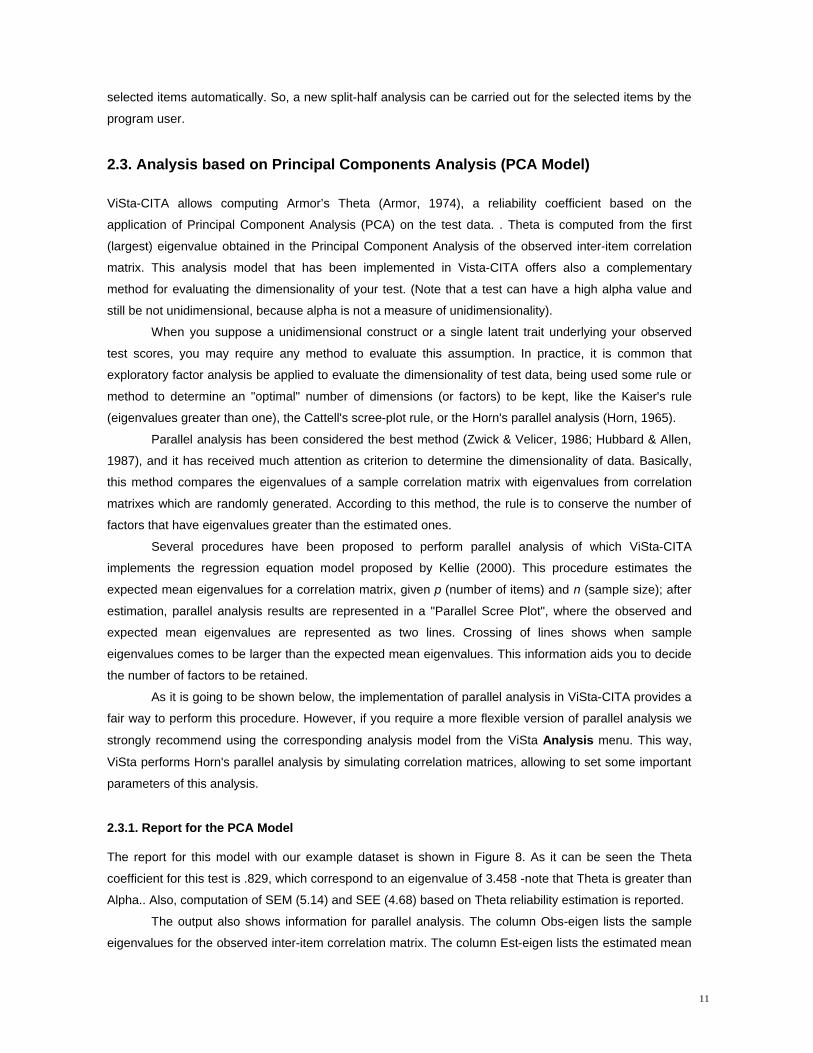
2.3.1. Report for the PCA Model

The report for this model with our example dataset is shown in Figure 8. As it can be seen the Theta

coefficient for this test is .829, which correspond to an eigenvalue of 3.458 -note that Theta is greater than

Alpha.. Also, computation of SEM (5.14) and SEE (4.68) based on Theta reliability estimation is reported.

The output also shows information for parallel analysis. The column Obs-eigen lists the sample

eigenvalues for the observed inter-item correlation matrix. The column Est-eigen lists the estimated mean

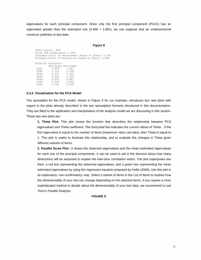
12

eigenvalues for each principal component. Since only the first principal component (PCA1) has an

eigenvalue greater than the estimated one (3.458 > 1.861), we can suppose that an unidimensional

construct underlies to test data.

Figure 8 Theta value: .829 First PCA eigenvalue: 3.458 Standard error of measurement based on Theta: 5.144 Standard error of estimation based on Theta: 4.685 Parallel Analysis: Obs-eigen Est-eigen PCA1 3.458 1.861 PCA2 1.314 1.599 PCA3 0.732 1.368 PCA4 0.584 1.165 PCA5 0.459 0.987 PCA6 0.270 0.832 PCA7 0.183 0.699

2.3.2. Visualization for the PCA Model

The spreadplot for the PCA model, shown in Figure 9 for our example, introduces two new plots with

regard to the plots already described in the two spreadplots formerly introduced in this documentation.

They are fitted to the application and interpretation of the analysis model we are discussing in this section.

These two new plots are:

1. Theta Plot: This plot shows the function that describes the relationship between PCA

eigenvalues and Theta coefficient. The horizontal line indicates the current values of Theta. . If the

first eigenvalue is equal to the number of items (maximum value can take), then Theta is equal to

1. This plot is useful to illustrate this relationship, and to evaluate the changes in Theta given

different subsets of items.

2. Parallel Scree Plot:: It shows the observed eigenvalues and the mean estimated eigenvalues

for each one of the principal components. It can be used to aid in the decision about how many

dimensions will be assumed to explain the inter-item correlation matrix. The plot superposes two

lines: a red line representing the observed eigenvalues, and a green line representing the mean

estimated eigenvalues by using the regression equation proposed by Kellie (2000). Use this plot in

an exploratory -non-confirmatory- way. Select a subset of items in the List of Items to explore how

the dimensionality of your test can change depending on the selected items. If you require a more

sophisticated method to decide about the dimensionality of your test data, we recommend to use

‘Horn’s Parallel Analysis’.

FIGURE 9

13

3. ALGORITHMS

3.1. Cronbach’s Alpha coefficient:

−

−= ∑ =

2

211

1 X

iki

S

S

kk

α

Where k is the number of items, 2iS is the variances of item i, and 2

XS is the total score variance.

3.2. Spearman-Brown prophecy formula:

'

'' )1(1

'XX

XXXX n

nρ

ρρ

−+=

Where n is the number of times the test length is increased and 'XXρ is the reliability coefficient. 3.3. Spearman-Brown’s adapted to the split-Half case: Equal length:

'

'' 1

2'

XX

XXXX ρ

ρρ

+=

Unequal length:

221

2'

221

2'

2'

4'

2'

'/)1(2

/)1(4'

kkk

kkk

XX

XXXXXXXXXX

ρ

ρρρρρ

−

−++−=

Where 1k and 2k are the number of item in each part.

14

3.4. Guttman-Flanagan coefficient (Split-Half method):

+−= 2

22

21

' 12total

XX SSS

ρ

Where S21 and S2

2 are the respective variances of the two Halves. 3.5. Armor’s Theta:

−

−=

1

11

1 λθ

kk

Where 1λ is the largest eigenvalue of the sample correlation matrix. 3.6. SEM and SEE

Standard error of measurement:

'2 1 XXXSSEM ρ−=

Standard error of estimation:

''2 1 XXXXXSSEE ρρ−=

4. REFERENCES Castañeiras & Belloch, 1997 Armor, D. J. (1974). Theta reliability and factor scaling. In: Costner, H. L. (eds.), Sociological Methodology, 17-

50. SF: Jossey-Bas. Brown, W. (1910). Some experimental results in the correlation of mental abilities. British Journal of Psychology,

3, 296-322. Cronbach, L. J. (1951). Coefficient alpha and the internal structure of tests. Psychometrika, 16, 297-334. Gulliksen, H. (1950). Theory of mental tests. New York: John Wiley. Horn, J.L. (1965). A rationale and technique for estimating the number of factors in factor analysis.

Psychometrika, 30, 179-185. Keeling, K. (2000) A Regression Equation for Determining the Dimensionality of Data. Multivariate Behavioral

Research, 35, 457-468 Lord, F. M. & Novick, M. R. (1968). Statistical theories of mental test scores. Reading, MA: Addison-Wesley. Spearman, C. (1910). Correlation calculated from faulty data. British Journal of Psychology, 3, 271-295. Zwick, W. R. y Velicer, W. F. (1986). Comparison of five rules for determining the number of components to

retain. Psychological Bulletin, 99, 432-442. Hubbard, R. & Allen, S. J. (1987). An empirical comparison of alternative methods for principal component

extraction. Journal of Business Research, 15, 173-190.