Local wind forcing of the Monterey Bay area inner shelf

ARTICLE IN PRESS

0278-4343/$ - se

doi:10.1016/j.cs

�Correspondisity of Californ

California 9506

E-mail addre

Continental Shelf Research 25 (2005) 397–417

www.elsevier.com/locate/csr

Local wind forcing of the Monterey Bay area inner shelf

Patrick T. Drakea,�, Margaret A. McManusb, Curt D. Storlazzic

aLong Marine Lab., University of California, Santa Cruz, CA, USAbDepartment of Oceanography, University of Hawaii at Manoa, Honolulu, HI, USA

cUS Geological Survey, Coastal and Marine Geology Program, Pacific Science Center, Santa Cruz, CA, USA

Received 18 June 2003; received in revised form 16 September 2004; accepted 1 October 2004

Abstract

Wind forcing and the seasonal cycles of temperature and currents were investigated on the inner shelf of the

Monterey Bay area of the California coast for 460 days, from June 2001 to September 2002. Temperature

measurements spanned an approximate 100 km stretch of coastline from a bluff just north of Monterey Bay south to

Point Sur. Inner shelf currents were measured at two sites near the bay’s northern shore. Seasonal temperature

variations were consistent with previous observations from the central California shelf. During the spring, summer and

fall, a seasonal mean alongshore current was observed flowing northwestward in the northern bay, in direct opposition

to a southeastward wind stress. A barotropic alongshore pressure gradient, potentially driving the northwestward flow,

was needed to balance the alongshore momentum equation. With the exception of the winter season, vertical profiles of

mean cross-shore currents were consistent with two-dimensional upwelling and existing observations from upwelling

regions with poleward subsurface flow. At periods of 15–60 days, temperature fluctuations were coherent both

throughout the domain and with the regional wind field. Remote wind forcing was minimal. During the spring

upwelling season, alongshore currents and temperatures in the northern bay were most coherent with winds measured

at a nearby land meteorological station. This wind site showed relatively low correlations to offshore buoy wind

stations, indicating localized wind effects are important to the circulation along this stretch of Monterey Bay’s inner

shelf.

r 2004 Elsevier Ltd. All rights reserved.

Keywords: Coastal upwelling; Inner shelf; Wind-driven currents; Ekman transport

e front matter r 2004 Elsevier Ltd. All rights reserve

r.2004.10.006

ng author. Long Marine Laboratory, Univer-

ia, Santa Cruz, 100 Shaffer Road, Santa Cruz,

0, USA.

ss: [email protected] (P.T. Drake).

1. Introduction

The inner continental shelf, defined here aswater depths shoreward of 30m, plays a criticalrole in both coastal circulation and the dynamicsof marine ecosystems. Measurements show wind-driven upwelling on the US west coast, which

d.

www.elsevier.com/locate/csr

ARTICLE IN PRESS

Fig. 1. Study site showing the Monterey Bay area of the

California coast and locations of wind stations (N12, LML,

N42, M1, AQ, SUR, N28, N11, N53, N25), temperature

moorings (SHB, TPT, M1, HMS, SWC, PTS) and ADCP

P.T. Drake et al. / Continental Shelf Research 25 (2005) 397–417398

eventually feeds the elevated biological productivityfound there, will be strongest over the inner shelf,closest to the shore (Huyer, 1983; Winant et al.,1987). These measurements are consistent withtheoretical treatments of coastal upwelling (Allen,1975), which predict that upwelling will be mostpronounced within the baroclinic Rossby radius ofthe coast, roughly within 10 km of the shoreline.Satellite images (Kosro et al., 1991) reveal theimportance of upwelling on the inner shelf to thegrowth of the larger-scale upwelling front andcoastal transition zone further offshore.

To gain a better understanding of the upwellingand wind forcing on the inner shelf, long-termtemperature and current measurements made inthe Monterey Bay region of the US west coastwere studied and compared to a variety of windmeasurements. The observations and analysissummarized here were performed at the Universityof California, Santa Cruz, and were supported bythe Partnership for Interdisciplinary Studies ofCoastal Oceans (PISCO), a multi-institutionalresearch program. Observations spanned well over1 year, from 4 June 2001 to 7 September 2002. Thespatial extent of the study was approximately100 km, from a bluff just north of Monterey Baysouth to Point Sur.

current profilers (SHB, TPT). Water depth of the PISCO inner

shelf stations (SHB, TPT, HMS, SWC, PTS) was �20m.

Isobath contour interval is 10m for water depths o200m and

100m for depths 4200m.
2. Methods
2.1. Instrumentation

The study encompassed five inner shelf moor-ings north of, inside, and to the south of MontereyBay (Fig. 1, Table 1). Located in an approximatewater depth of 20m, all five shelf mooringsmeasured temperature at three depths, referred toas bottom, middle, and top. Currents, measuredwith Acoustic Doppler Current Profilers (ADCPs),were also analyzed at the two northernmost sites(SHB and TPT). All inner shelf moorings weremaintained by the UCSC PISCO program. Sup-plementary temperature data from a deep-watermooring inside Monterey Bay (M1) and a varietyof wind data sets were also used to complement theanalysis. Maintained by the Monterey Bay Aqua-rium Research Institute (MBARI), the M1 moor-

ing is located in a nominal water depth of 1600min the heart of the Monterey Submarine Canyon.Only temperature from M1’s 10m depth will bepresented here, as this depth was available for bothcalendar years. Wind data from 10 different siteswere employed in the analysis (Table 2). Both land(LML, AQ, SUR) and offshore buoy windstations, including M1, were used. All buoy windstations, with the exception of M1, were main-tained by the National Data Buoy Center. Land-based wind measurements were made availablefrom the Monterey Bay Aquarium (AQ), UCSC’sLong Marine Lab (LML) and the Department ofMeteorology at the Naval Postgraduate School,which maintains a meteorological station at thePoint Sur Naval Station (SUR).

ARTICLE IN PRESS

Table 1

Mooring locations and instrument depths

Name ID Water

depth (m)

Lat., 1N Lon., 1W Thermistor

depths (m)

ADCP

rangeaMajor (y-)

axis (1T)

Sand Hill Bluff SHB 20 36.97 122.16 3, 11, 19 2–17 327

Terrace Point TPT 18 36.94 122.08 4, 10, 17 3–15 295

M1 M1 1600 36.75 122.03 10 — —

Hopkins Marine Station HMS 18 36.62 121.90 3, 10, 17 — —

Stillwater Cove SWC 21 36.56 121.94 5, 12, 20 — —

Point Sur PTS 20 36.28 121.87 4, 10, 18 — —

All depths in meters below MLLW. See Fig. 1 for site locations.aRefers to valid measurement depths for upward-looking ADCPs.

Table 2

Wind measurement stations

Station name ID Lat., 1N Lon., 1W Major (y)

axis (1T)

y (km)a

NDBC Buoy 46012, Half Moon Bay N12 37.36 122.88 333 85

Long Marine Lab LML 36.95 122.07 282 25

NDBC Buoy 46042, Monterey Bay N42 36.75 122.42 317 0

M1 Buoy, Monterey Bay M1 36.75 122.03 315 0

Monterey Bay Aquarium AQ 36.62 121.90 308 �20

Point Sur Naval Station SUR 36.30 121.89 334 �70

NDBC Buoy 46028, Cape San Martin N28 35.74 121.89 315 �135

NDBC Buoy 46011, Santa Maria N11 34.88 120.87 326 �280

NDBC Buoy 46053, Santa Barbara East N53 34.24 119.85 278 �420

NDBC Buoy 46025, Santa Monica Basin N25 33.75 119.08 293 �510

aRefers to approximate alongshore distance relative to N42. Distances were estimated roughly from NOAA nautical charts.

P.T. Drake et al. / Continental Shelf Research 25 (2005) 397–417 399

Temperatures at the inner shelf sites weremeasured with Onset StowAway-XTI temperatureloggers. The Onset sensors have a precision of�0.2 1C. Velocities were measured with bottom-mounted, upward-looking RD Instruments600 kHz Workhorse Sentinel ADCPs. The verticalresolution of the ADCP was 1m at all sites. Thenominal uncertainty in the ADCP hourly mea-surements due to Doppler noise was �0.2 cm/s.Thermistor depths and the valid ADCP range foreach site are shown in Table 1. ADCP depths referto bin centers.

2.2. Data selection and processing

The overall time period selected for study waschosen for its comprehensive wind, ADCP and

temperature data coverage. Using the oceano-graphic ‘‘seasons’’ identified by Largier et al.(1993) for the northern California coast, the studyperiod was further divided into four separatesubperiods for statistical analysis (Table 3). Thesesubperiods correspond to the spring upwellingseason, the fall relaxation season, the winter stormseason and a complete year surrounding the threeseasons. Each of the three seasons spans 108 daysand was delineated based on the timing of thespring transition, seasonal temperature minimumsand maximums, and the avoidance of data gaps.Throughout this study, calendar days are num-bered consecutively, with day 0 starting 12 a.m.Pacific Standard Time 1 January 2000. Some databeyond the bounds of the study period (notpresented for the sake of brevity) were used to

ARTICLE IN PRESS

Table 3

Study sub-periods used in statistical analysis

Season or demarcation Dates Day numbers

2001–2002 year 20 July 2001–20 July 2002 566–931.25

Fall 2001, relaxation season 24 July 2001–9 November 2001 570–678

Winter 2001–2002, storm season 27 November 2001–15 March 2002 696–804

Spring 2002, upwelling season 31 March 2002–17 July 2002 820–928


help determine the timing of the seasonal max-imums and minimums discussed in Section 3.1. Inmany ways, the data were consistent with previousobservations on the California coast (Section 3.1.).However, it is emphasized here that these three108-day seasons may not necessarily be genericrepresentations of fall, winter, and springtimeconditions in the area.

Except for use in the Richardson numbercalculation (Section 3.1.), all data were hourlyaveraged and low-passed filtered (half-powerperiod of 36 h). When possible, data gaps werefilled with linear regressions from significantlycorrelated sensors on common moorings. Largerecord gaps of the deepest ADCP bin at both SHBand TPT (the bin occasionally failed due to afirmware problem) were filled using a regressionfrom a neighboring bin. A 44-day gap in PTSbottom temperature during spring 2002 and a 15-day gap in HMS top temperature during fall of2001 were filled with a linear regression from theirrespective moorings’ middle sensors. However,most gaps were smaller (o2 days) and could notbe filled with regressions from neighboring sen-sors. The remaining gaps were filled with low-passed white noise with the same mean and low-passed variance as the surrounding season or year.The data set contained only one substantial gapfilled with noise: a 16-day gap in SHB current infall 2001. Unless explicitly stated otherwise, allstatistical calculations refer to the time periods inTable 3, with the data low-passed and gaps filledas described above.

The principal axes (Kundu and Allen, 1976)were determined for both winds and depth-averaged currents, and the major axes are listedin Tables 1 and 2. The calculation was based onthe entire year, 20 July 2001–20 July 2002 (365.25

days), surrounding the three seasons. The direc-tions in Tables 1 and 2 define the positive y-axis(alongshore) for both winds and currents. Thisgives the positive alongshore direction as roughlynorthwestward at all sites. Correspondingly, thepositive x-axis points roughly northeastward(onshore) at all sites. The major axes of thecurrents and winds generally followed the iso-baths, as would be expected from topographicsteering close to the coastline and coastal moun-tains.A linear trend was removed from all data before

making standard deviation and correlation calcu-lations. Effective degrees of freedom for correla-tion significance levels were determined using theintegral time scale of the data, as suggested byEmery and Thomson (1997, Chapter 3), and werecalculated by integrating the autocorrelation outto the first zero-crossing. All coherence calcula-tions were made by subdividing the data into 60-or 18-day increments, removing a linear trend,multiplying by a Hanning window and block-averaging with a 50% overlap. Significance levelson the coherence estimates were determined usingthe Goodman formula (Thompson, 1979), withaccount made for averaging overlapping, corre-lated transforms as prescribed by Harris (1978).To keep the plots uncluttered error bars are notshown for the phase. The standard deviation of thephase varies inversely with the coherence (Bendatand Piersol, 2000, Chapter 9). To give some senseof the uncertainty in the phase estimates, when thecoherence is significantly different from zero, thestandard deviation of the phase is approximately201 or less. Data for power spectra calculationswere subdivided into three 54-day increments with50% overlap, detrended, and multiplied by aHanning window.

ARTICLE IN PRESS

550 600 650 700 750 800 850 900 950

101214

Day Number

PTS Temps.

101214

SWC Temps.

101214

HMS Temps.

101214

M1 Temp.

101214

TPT Temps.

101214

o Co C

o Co C

o Co C

SHB Temps.

-200

20

cm/s

SHB Current

-100

10

m/s

N42 Wind

Jul2

001

Aug

2001

Sep

2001

Oct

2001

Nov

2001

Dec

2001

Jan2

002

Feb

2002

Mar

2002

Apr

2002

May

2002

Jun2

002

Jul2

002

Aug

2002

Sep

2002

Fig. 2. Monterey Bay area low-frequency winds, currents, and

bottom and top water temperatures, June 2001–September

2002. Shaded areas denote distinct oceanographic seasons:

spring upwelling, fall relaxation, and winter storm. For the stick

plots, northward is toward the top of the page, and a vectors’

magnitude can be scaled on the y-axis. SHB current is a depth-

average. Monthly tick marks (top x-axis) fall on the first of the

month.


3. Results

3.1. General seasonality

Seasonal wind trends for N42 and LML (Figs. 2and 3) were generally consistent with previousreported observations along the central Californiacoast (Largier et al., 1993; Strub et al., 1987).Because of the interaction of large-scale atmo-spheric pressure systems (Lentz, 1987), winds arepredominantly southeastward (equatorward) dur-ing spring, summer, and early fall (March–November in 2001 and 2002). This southeastwardwind is episodically interrupted by brief relaxa-tions lasting approximately 2–7 days, when thewind either weakens or turns northwestward.During the winter storm season, winds becomemore variable and their seasonal mean (108-dayaverage) weakens. This can be seen both in thetime history plots (Fig. 3) and basic statistics(Table 4a). Note the decrease in the mean andincrease in the standard deviation for both LMLand N42 during winter. The other wind sites in theMonterey Bay area, N12, M1, AQ, SUR, N28 (notshown), displayed a similar pattern of relativelystrong southeastward winds during spring, sum-mer and fall and a reduced mean in winter. During2001 and 2002 at N42, monthly means of thissoutheastward wind peaked in June (monthlyaverages not shown). Regardless of season, theabsolute magnitude of the wind was significantlyless at the land stations LML and AQ compared tothe NDBC buoys (Fig. 3). The wind velocities werenot adjusted for differing sensor heights; this wouldhave exaggerated the land/buoy difference, as thesensors were higher at the land stations. Asdiscussed by Halliwell and Allen (1987), increasedfriction over land and/or the varying strength of thediurnal seabreeze/landbreeze with increasing dis-tance from shore may be responsible for the effect.

Winds and currents were generally highlypolarized along their respective major axes. Thedegree of polarization can be quantified with theellipticity, defined here as major-axis-variance/minor-axis-variance. Ellipticities were typicallywell above 50 for currents and ranged from 4 to12 for winds when calculated over the completeyear. LML was an exception and showed the least

polarization, ellipticity �2. Relative to spring andfall, winds and currents were less polarized in thewinter, typically by a factor of 2–3 for winds and1.5–2 for currents. The directions of the major axesalso varied slightly from season to season(Dyo101), with the biggest differences found withrespect to the winter orientations. However, theresults presented in this study were not sensitive tosuch small changes in axes orientation.All temperature measurements (Fig. 2) showed

seasonal behavior consistent with previous obser-vations made within Monterey Bay (Graham andLargier, 1997) and over the central and northernCalifornia shelf (Largier et al., 1993; Lentz, 1987;Strub et al., 1987). Monthly means of bottom and

ARTICLE IN PRESS

Table 4

Fall 2001 Winter 2001–2002 Spring 2002

Mean Std Mean Std Mean Std

(a) Basic seasonal current and wind statisticsa

Wind or current station

LML v (m/s) �1.3 1.0 �0.1 1.8 �2.7 1.8

LML u (m/s) 0.4 0.5 �0.2 1.8 0.5 0.8

N42 v (m/s) �4.1 3.7 �2.2 5.6 �5.6 4.2

N42 u (m/s) 0.5 0.6 0.0 2.1 1.0 0.8

SHB v (cm/s) 4.8 7.1 �0.3 7.3 4.8 7.7

SHB u (cm/s) �0.2 0.7 �0.6 1.1 �0.3 0.7

TPT v (cm/s) 5.4 5.7 0.4 5.7 6.7 4.2

TPT u (cm/s) 0.4 0.7 0.2 0.8 0.4 0.6

(b) Basic seasonal temperature statisticsb

Temperature station

SHB top 13.0 0.6 11.6 0.7 11.2 0.9

SHB bottom 11.6 0.5 11.4 0.6 10.0 0.6

TPT top 13.5 0.5 11.6 0.7 11.8 0.8

TPT bottom 12.0 0.5 11.4 0.6 10.4 0.6

M1 10m 12.8 0.6 11.9 0.6 11.0 0.5

HMS top 13.6 0.7 12.1 0.8 12.5 0.7

HMS bottom 11.9 0.7 11.6 0.7 10.7 0.6

SWC top 12.2 0.8 11.5 0.7 10.7 0.7

SWC bottom 11.5 0.8 11.2 0.7 9.9 0.7

PTS top 12.2 0.9 11.7 0.7 10.2 0.9

PTS bottom 11.4 0.8 11.4 0.7 9.7 0.8

aCurrents statistics refer to depth-averages. See Tables 2 and

3 for axis definitions.bAll temperature statistics in 1C.

550 600 650 700 750 800 850 900 950

101214

Day Number

o C

SHB Temps.

-303

cm/s

TPT U

-20

0

20

cm/s

TPT V

-10

-5

0

5

cm/s

SHB U

-200

20

cm/s

SHB V

-100

10

m/s

N42 V, LML V-505

m/s

Jul2

001

Aug

2001

Sep

2001

Oct

2001

Nov

2001

Dec

2001

Jan2

002

Feb

2002

Mar

2002

Apr

2002

May

2002

Jun2

002

Jul2

002

Aug

2002

Sep

2002

Fig. 3. Low-frequency winds and currents from northern

Monterey Bay. Shaded areas denote oceanographic seasons

defined in text. LML winds (dotted) are scaled on the right-

hand axis. v is alongshore velocity component, u the cross-

shore. At (SHB, TPT) dotted lines represent near-surface (2,

3m depth) currents, and solid lines represent near-bottom (17,

15m depth) currents. Monthly tick marks (top x-axis) fall on

the first of the month. Top and bottom SHB temperatures are

also shown for comparison of annual temperature cycle (see

Fig. 2).


top temperatures displayed a minimum in spring(April in 2001 and May or June in 2002), a monthor two after the wind turned steadily south-eastward. During both 2001 and 2002, bottomand top temperatures then steadily rose through-out the remaining spring and summer, withmonthly mean bottom temperatures reaching amaximum in November. Monthly mean toptemperatures either peaked in November withbottom temperatures, or reached a maximumearlier in summer (September for TPT in 2001and August for HMS in 2002). Temperaturesdeclined during the winter storm season (Decem-ber to February), when the water column was well-mixed.

Mean temperatures were highest at HMS andTPT, sites in and near Monterey Bay’s southernand northern bights, respectively (Table 4b).During spring and fall, SHB temperatures wereconsistently below TPT temperatures at all mea-sured depths. SWC and PTS, south of the bay,were consistently the coolest sites. The relativelywarm temperatures at TPT were consistent withthe persistent warm temperature zone, or ‘‘upwel-ling shadow,’’ previously observed in MontereyBay’s northern bight (Graham and Largier, 1997).The temperature stratification at most sites peakedin mid-summer (June and July in 2001, and Julyand August in 2002). Stratification was highest atHMS, with typical top-sensor-to-bottom-sensor,mid-summer, daily values of �0.25–0.35 1C/m.Values were slightly less at TPT and SHB, butsubstantially less (�0.05–0.1 1C/m) south of Mon-terey Bay at SWC and PTS. These peak summer-

ARTICLE IN PRESS


time stratification values are about two or threetimes the fall (108-day) averages. These verticaltemperature gradients are consistent with priorinner shelf measurements from within MontereyBay (�0.2 1C/m, Graham and Largier, 1997). Butnote that the stratification reported here isrelatively large compared to other reported sum-mertime measurements at similar depths on thenorthern California inner shelf (�0.02 1C/m,Lentz, 1994), and deeper nearby shelf measure-ments (�0.01 1C/m, Ramp and Abbott, 1998). Themeasurements reported here are closer to thosereported for the Southern California Bight(Pringle and Riser, 2003). The relatively largestratification values indicate that vertical mixingmay have been reduced in the water column’sinterior, despite the shallow overall water depth.Bulk gradient Richardson number (Ri) calcula-tions, based on hourly, unfiltered thermistor andADCP data at SHB and TPT show much scatter,but give RiX0.25. These calculations, thoughimprecise due to the separation of the sensors,suggest a near-inviscid interior existed with rela-tively thin (�1–5m) top and bottom boundarylayers.

Throughout the spring, summer and early fall,the temperature record at all inner shelf sites waspunctuated by �0.5–3 1C increases in temperaturelasting 2–20 days. These temperature fluctuationswere observed throughout the water column andare shown in Section 3.4 to be caused byrelaxations of the predominantly southeastwardwind stress. With the exception of at SWC, theserelaxation events also noticeably strengthened thetemperature stratification, with top sensors experi-encing more warming. At SWC, the fluctuationswere of approximately equal magnitude through-out the water column.

The current records displayed high variabilityyear-round, with standard deviations of bothalongshore (v) and cross-shore (u) depth-averagedvelocities usually larger than their respectiveseasonal means (Table 4a). But a relativelyconsistent, northwestward (poleward) mean flowwas observed at both SHB and TPT during springand fall (Fig. 3). This northwestward flow relaxedto a near-zero mean during winter. The north-westward flow is consistent with existing measure-

ments in northern Monterey Bay. Prior long-termcurrent observations at SHB and near TPT displaynorthwestward means (Breaker and Broenkow,1994; Storlazzi et al., 2003). High-frequency radarmeasurements show cyclonic, basin-scale surfaceflow inside the bay, northwestward near TPT, inlate summer and fall (Paduan and Rosenfeld,1996). And a smaller-scale, cyclonic flow pattern inthe bay’s northern bight has been inferred basedon the hydrgography of the upwelling shadow(Graham and Largier, 1997), implying northwest-ward near-surface flow near TPT.At SHB, monthly means of depth-averaged

alongshore flow displayed maximums in May of2001 and July of 2002 (monthly averages notshown). At TPT, the maximums were in August of2001 and June of 2002. (Compare with N42’s Junemaximums in southeastward wind velocity.) Theannual signal in alongshore currents was approxi-mately p radians out of phase with the annualwind signals at N42 and LML, with a seasonalmean northwestward current flowing in directopposition to a southeastward wind stress duringspring and fall (Fig. 3 and Table 4a). It is commonfor mean currents on the central and northernCalifornia shelf to flow northward in opposition tosouthward or southeastward winds (Chelton et al.,1988; Largier et al., 1993; Lentz, 1994; Ramp andAbbott, 1998; Strub et al., 1987), especially duringlate summer and winter. But this northward flow isusually preceded by a period of southward flowduring the spring, at least at the surface. Previousauthors have invoked a northward-forcing (i.e.negative) alongshore pressure gradient to explainthese seasonal periods of northward flow duringtimes of southward wind stress (Largier et al.,1993; Lentz and Trowbridge, 2001).

3.2. Seasonal scaling

The unusual wind-current phasing and otherseasonal dynamics in northern Monterey Bay wereinvestigated by scaling the various terms in themomentum equations, with calculations madedirectly from the data when possible. An along-shore pressure gradient was found to be of primaryimportance here as well. Using the followingnotation to define the linear and non-linear

ARTICLE IN PRESS


transports,

M ðu;vÞ ¼

Z Z

�H

ðu; vÞ dz;

M ðuu;vvÞ ¼

Z Z

�H

ðuu; vvÞ dz;

Muv ¼

Z Z

�H

uv dz;

the depth-integrated alongshore momentum equa-tion can be written:

Mvt þ Muv

x þ Mvvy þ fMu

¼ �gH2

2r0ry � gðH þ ZÞZy þ r�1

0 tyw � r�1

0 tyb: ð1Þ

Here, u and v are the cross- and alongshorecomponents of velocity, r is the perturbationdensity, r0 is a reference density, Z is the seasurface height, ty

ðw;bÞ are the wind and bottomstresses, H is the water depth, and subscripts referto differentiation. The pressure has been linearizedabout z ¼ 0; the still sea surface. Horizontaldensity gradients were assumed to be depth-independent. With the same assumptions andnotation, the depth-integrated cross-shore momen-tum equation becomes

Mut þ Muu

x þ Muvy � fMv

¼ �gH2

2r0rx � gðH þ ZÞZx þ r�1

0 txw � r�1

0 txb : ð2Þ

Table 5

Dynamic scaling

Alongshore depth-integrated momentum equation

Mvt Muv

x Mvvy fMu

�

Fall �7� 10�8 — 5� 10�6 1� 10�6�

Winter 3� 10�7 — 6� 10�6�5� 10�6

�

Spring 2� 10�7 — 7� 10�6�2� 10�6

�

Cross-shore depth-integrated momentum equation

Mut Muu

x Muvy �fMv

�

Fall �2� 10�8 — 9� 10�6�8� 10�5 —

Winter 4� 10�8 — 6� 10�6�2� 10�6 —

Spring 3� 10�8 — 1� 10�5�9� 10�5 —

Values are seasonal means. Units are m2/s2.

The seasonal averages of the measured terms aregiven in Table 5. The values are representative ofseasonal and perhaps monthly timescales,T�30–108 days. Wind stresses were calculatedusing the method of Large and Pond (1981) usingdata from LML. Bottom stresses were estimatedusing the velocity in the lowest ADCP bin, aquadratic drag law, and a drag coefficient of5� 10�3 (Lentz, 1994). Velocities used to estimatethe transports and bottom stresses were firstrotated into a common reference frame withalongshore (y) axis oriented along a line joiningTPT and SHB, positive toward SHB. Transportsand stresses were then either averaged or differ-enced between the two sites, centering the esti-mates. This increased their accuracy, butprecluded the calculation of cross-shore gradients.The portions of the water column unresolved bythe ADCP were ignored in the transport calcula-tions. The baroclinic pressure gradient, the firstterm on the right-hand-side of Eq. (1), wasestimated using the equation of state of seawater,the average temperature difference between thethree sensors on each mooring, an assumedsalinity of 33.5 PSU (Breaker and Broenkow,1994), and zero pressure.No obvious, simple balance is apparent in the

alongshore momentum equation during winter,but during fall and spring a dominant balanceinvolving the wind stress and pressure gradientscan be inferred. There is no measured term with

1=2gH2r�10 ry

�gðH þ ZÞZy r�10 ty

w �r�10 ty

b

2� 10�5 — �1� 10�5�6� 10�6

2� 10�6 — �2� 10�6 2� 10�6

2� 10�5 — �3� 10�5�9� 10�6

1=2gH2r�10 rx

�gðH þ ZÞZx r�10 tx

w �r�10 tx

b

— 4� 10�6 9� 10�7

— 4� 10�6 5� 10�7

— 8� 10�6�4� 10�7

ARTICLE IN PRESS

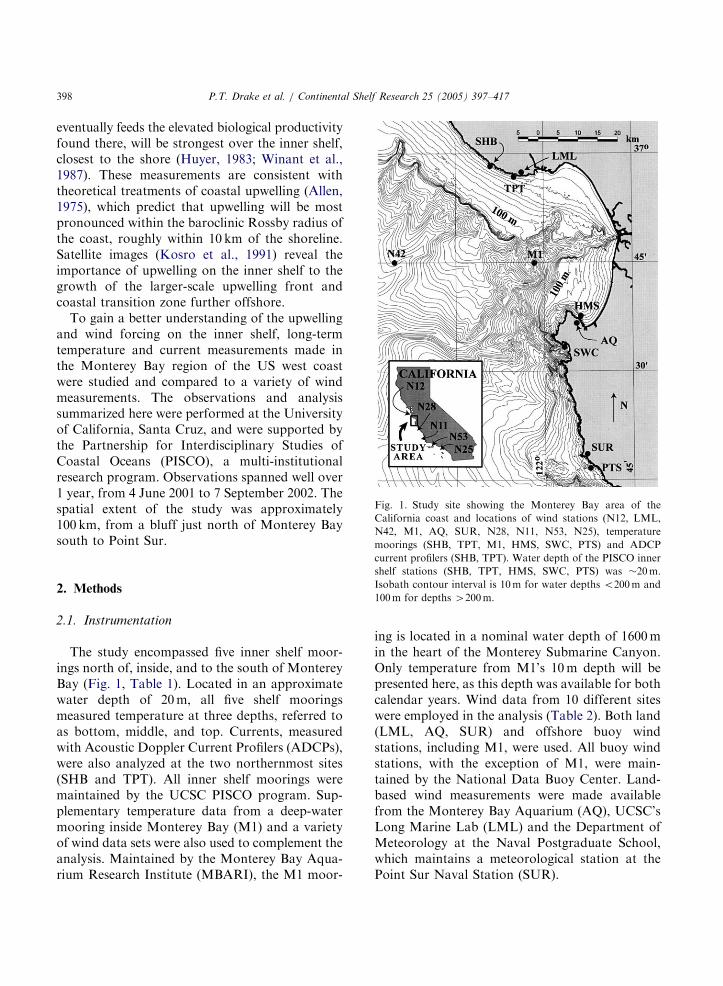
Fig. 4. Seasonal means of alongshore (v) and cross-shore (u)

velocities. Top of panel represents Mean Lower Low Water

(MLLW).


the proper sign and size to balance the combina-tion of the wind stress and baroclinic pressuregradient on the right-hand side of Eq. (1) (Table5). The magnitude of the wind stress is likely anunderestimate, as it was based on data from a landstation (Halliwell and Allen, 1987). The cross-shore advection term Muv

x was not measureddirectly, but it can be easily scaled. Using across-shore length scale for the alongshore currentof 10 km, given the observed bottom slope, andassuming currents will approximately follow iso-baths, Muv

x will scale like �1� 10�6m2/s2. Thisleaves only the unmeasured barotropic pressuregradient available to balance the wind stress andbaroclinic pressure gradient in Eq. (1). Such apressure gradient corresponds to a sea-surfaceslope of 5� 10�7, with the sea surface higher to thesoutheast, inside the bay.

Turing to the cross-shore momentum Eq. (2),the dominant balance appears to be geostrophic infall and spring, as traditionally assumed, but notso in winter. In fall and spring, the Coriolisacceleration is by far the largest measured term. Itcan only be balanced by one of the pressure termsor the cross-shore advective term Muu

x : This termwas also not directly measured, but scaling it withthe same assumptions as Muv

x yields a value of�1� 10�6m2/s2, much too small to balance theCoriolis acceleration. Previous hydrographic mea-surements near TPT suggest that the cross-shorebaroclinic pressure gradient is positive (rxo0),with warmer water closer to shore (Graham andLargier, 1997). If this is the case, only thebarotropic cross-shore pressure gradient can bal-ance the Coriolis term in fall and spring. Thisimplies positive sea surface setup at the coast,despite the mean southeastward winds observed atLML and N42 and their implied offshore Ekmantransport. In winter, the Coriolis acceleration isnot a dominant term due to the near-zero meanalongshore current, and there is apparently nosimple geostrophic balance, at least not on theseasonal timescale.

3.3. Mean velocity profiles

Seasonal mean velocity profiles (Fig. 4) weresimilar at SHB and TPT. But alongshore spring

profiles at both sites differed substantially fromprevious observations made on the Californiacoast (Winant et al., 1987; Largier et al., 1993)and at other upwelling regions (Smith, 1981). Asnoted in Section 3.1, alongshore mid-shelf currentsin upwelling regions during spring and earlysummer are typically equatorward near the sur-face, although poleward subsurface flow may bepresent. Spring profiles observed here were north-westward (poleward) at all depths. However, fallalongshore profiles at SHB and TPT were similarto earlier fall shelf observations made in northernCalifornia (Lentz and Trowbridge, 2001), display-ing northwestward flow at all depths and a mid-depth maximum. During all seasons, the verticalshear in the alongshore current was slightly largerat TPT relative to SHB. The winter displayedsurprisingly small alongshore means at all depthswith relatively little shear, especially at SHB.Cross-shore profiles were comparatively invar-

iant between seasons and were consistent withprevious shelf observations from regions withpoleward subsurface shelf flow (Smith, 1981).Cross-shore profiles are also consistent with atwo-dimensional conceptualization of upwelling,where offshore Ekman transport at the surface,caused by a mean equatorward (southeastward)wind, is balanced by a compensatory onshore flow

ARTICLE IN PRESS

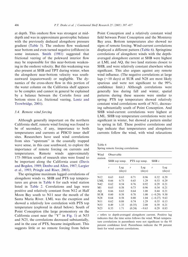
Table 6

Spring remote forcing correlations

Wind

station

Observable

SHB top temp. PTS top temp. SHB v

r Lag

(days)

r Lag

(days)

r Lag

(days)

N12 0.63 0.63 0.71 0.96 0.32 0.29

LML 0.66 0.75 0.43 1.29 0.53 0.29

N42 0.62 0.54 0.76 0.92 0.29 0.21

M1 0.65 0.58 0.73 0.96 0.34 0.21

AQ 0.66 0.63 0.64 1.08 0.44 0.21

SUR 0.60 0.58 0.78 1.00 (�0.29) 9.50

N28 0.64 0.58 0.80 1.04 (�0.27) 9.63

N11 0.62 0.88 0.74 1.29 0.35 0.13

N53 0.49 1.33 (0.35) 2.08 0.39 0.21

N25 0.35 1.71 (0.24) �9.63 0.29 0.83

v refers to depth-averaged alongshore current. Positive lag

indicates that the time series follows the wind. Wind–tempera-

ture correlations in parenthesis were not significant to the 95

percent confidence level. Parentheses indicate the 99 percent

limit for wind–current correlations.


at depth. This onshore flow was strongest at mid-depth and was in approximate geostrophic balancewith the previously deduced alongshore pressuregradient (Table 5). The onshore flow weakenednear bottom and even turned negative (offshore) insome instances. Smith (1981) suggested thatfrictional veering of the poleward interior flowmay be responsible for this near-bottom weaken-ing in the onshore velocity. But this weakening wasalso present at SHB and TPT during winter, whenthe alongshore near-bottom velocity was south-eastward (equatorward) or negligible. The dy-namics of the cross-shore flow in this portion ofthe water column on the California shelf appearsto be complex and cannot in general be explainedby a balance between the Coriolis force andbottom stress (i.e. frictional veering, Lentz andTrowbridge, 2001).

3.4. Remote wind forcing

Although generally important on the northernCalifornia shelf, remote wind forcing was found tobe of secondary, if any, importance to bothtemperatures and currents at PISCO inner shelfsites. Researchers have used wind correlationsfrom sites ‘‘upstream’’ in the coastally trappedwave sense, in this case southward, to explore theimportance of remote forcing on currents andtemperatures. Remote winds approximately175–500 km south of research sites were found tobe important along the California coast (Davisand Bogden, 1989; Denbo and Allen, 1987; Largieret al., 1993; Pringle and Riser, 2003).

The springtime maximum lagged correlations ofalongshore winds vs. SHB and PTS top tempera-tures are given in Table 6 for each wind stationlisted in Table 2. Correlations and lags werepositive and relatively constant from N12 at HalfMoon Bay south to N11 near the mouth of theSanta Maria River. LML was the exception andshowed a relatively low correlation with PTS toptemperature (explored in detail below). South ofPoint Conception (the large promontory on theCalifornia coast near the ‘‘Y’’ in Fig. 1) at N53and N25, the correlations decreased substantially,and in the case of PTS, became insignificant. Thissuggests little or no remote forcing from below

Point Conception and a relatively constant windfield between Point Conception and the MontereyBay area. Bottom temperatures also showed nosigns of remote forcing. Wind-current correlationsdisplayed a different pattern (Table 6). Springtimecorrelations of alongshore winds with the depth-averaged alongshore current at SHB were highestat LML and AQ, the two land stations closest toSHB, and were relatively constant elsewhere whensignificant. This also argues against any remotewind influence. (The negative correlations at largelags (�10 days) at SUR and N28 are most likelyspurious and were not significant to the 99%confidence limit.) Although correlations weregenerally less during fall and winter, spatialpatterns during these seasons were similar tospring: PTS top temperature showed relativelyconstant wind correlations north of N11, decreas-ing substantially south of Point Conception. AndSHB wind-current correlations were highest atLML. SHB top temperature correlations were notsignificant in winter, but showed a pattern similarto spring in fall. These positive correlations andlags indicate that temperatures and alongshorecurrents follow the wind, with wind relaxations

ARTICLE IN PRESS

Table 7

Spring wind–wind correlations

Wind station Wind station

LML N42 M1 AQ SUR N28

r Lag r Lag r Lag r Lag r Lag r Lag

N12 0.54 0.04 0.96 �0.04 0.91 �0.04 0.86 0.00 0.82 0.04 0.87 0.04

LML 1.00 0.00 0.49 �0.08 0.57 0.00 0.66 �0.04 0.42 �0.17 0.46 �0.17

N42 0.49 0.08 1.00 0.00 0.93 0.00 0.85 0.04 0.90 0.04 0.93 0.04

M1 0.57 0.00 0.93 0.00 1.00 0.00 0.91 0.00 0.89 0.04 0.91 0.00

AQ 0.66 0.04 0.85 �0.04 0.91 0.00 1.00 0.00 0.76 �0.04 0.82 �0.04

SUR 0.42 0.17 0.90 �0.04 0.89 �0.04 0.76 0.04 1.00 0.00 0.96 �0.04

N28 0.46 0.17 0.93 �0.04 0.91 0.00 0.82 0.04 0.96 0.04 1.00 0.00

N11 0.55 0.25 0.76 �0.25 0.77 �0.04 0.76 0.04 0.84 �0.13 0.87 �0.13

N53 0.56 0.21 (0.27) 4.67 0.33 4.42 0.38 �0.04 0.28 4.75 0.27 �0.96

N25 0.32 0.04 (�0.27) 1.04 0.29 4.25 0.29 10.8 �0.35 0.83 �0.31 1.33

Positive lags indicate the wind station in the column header leads. Lags are in days. Correlations in parenthesis were not significant to

the 99 percent confidence level.


resulting in warming at PTS and both warmingand northwestward velocity fluctuations at SHB.

High wind vs. wind correlations at short lags(Table 7) indicate a spatially coherent wind fieldexisted along California’s coast between HalfMoon Bay and Point Conception during spring.Most Monterey Bay area stations, LML, N42,M1, AQ, SUR, were well correlated (r � 0.8–0.9)with all stations north of Point Conception at lagsof a few hours. LML was an exception, displayingrelatively low (r � 0.5–0.6), although significant,correlations with its neighboring stations. Thisdifference in wind–wind correlation strength re-lative to LML (rE0.9 vs. rE0.5) was itselfsignificant to the 99% confidence level. Fall andwinter showed a pattern similar to that in spring:wind–wind correlations were high north of PointConception, except vs. LML, where they wererelatively low. These results are generally consis-tent with the findings of Halliwell and Allen(1987), who showed that most of the wind variancealong the US west coast was due to fluctuationswith alongshore wavelengths 4900 km. With theexception of LML, note the sharp drop incorrelation values of Monterey Bay area stationswith stations below Point Conception (N53 andN25), approximately 400–500 km to the south(Table 2). This distance is roughly consistent withthe �450 km spatial integral correlation scale

calculated for alongshore winds by Halliwell andAllen (1987). LML’s anomalously low correlationswith its neighbors suggest that the site has acomparatively short spatial integral correlationscale and that most of the station’s variancecannot be attributed to large-scale, regional(4500 km) wind fluctuations.

3.5. Temperature variability and its associated wind

forcing

The variance-preserving spectra of top andbottom temperatures at TPT and SWC are shownin Fig 5; the TPT temperature spectra are generallyrepresentative and sites inside or to the north ofthe bay (SHB, TPT, HMS), and the SWC spectraare generally representative of sites south of thebay (SWC, PTS). Temperature spectra were of twomain shapes: one shape displayed a single, broadpeak at long periods (20–50 days) and was typicalof the winter spectra at all sites. The second shapewas double-peaked with power concentrated atboth long periods (20–50 days) and short to mid-periods (3–15 days). This shape was typical of falland spring (e.g. TPT bottom, spring). The doublepeaks often merged together with averaging,creating a broad, single peak at long to mid-periods during fall and spring (e.g. SWC top, fall).Note the frequency resolution on these plots at

ARTICLE IN PRESS

Fig. 5. Variance-preserving power spectra of N42 and LML

alongshore winds and TPT and SWC temperatures for all three

seasons.


long periods, T420 days, where T is the period,was rather poor. Except for top temperatures atSHB, TPT and HMS, the temperature variancewas concentrated at periods longer than 10 days.The concentration of spectral power at lowfrequencies was especially pronounced duringwinter at the northern sites SHB, TPT and M1(SHB and M1 not shown), where there was almostno variance at periods shorter than 10 days. Thisfeature can be readily seen in the time domain(Fig. 2). Spring bottom and top spectra at TPTand SHB displayed a distinct peak between 3 and12 days. This peak is largest in the top temperaturespectra, where it dominates the overall tempera-ture variance. Top temperatures at SHB and TPT,the two northernmost sites, showed the largesthigh-frequency variance.

Wind spectra at N42 (Fig. 5) displayed a largevariation in the frequency distribution of variancebetween seasons and were generally dissimilarfrom the temperature spectra. For N42, a well-defined, relatively narrow peak near 12 daysdominates the fall spectra; a broad band of powerbetween 3 and 25 days defines the spring spectra,and the winter is characterized by two major lociof power, one near 3–5 days and another around25–50 days. LML’s wind spectra (Fig. 5) showedcomparatively less power at long periods, withmost of the winter and spring variance concen-trated at periods shorter than a week. Fall spectraat LML did share N42’s peak near 12 days, but thefeature was much less pronounced.The coherence of temperature between sites can

reveal the spatial scale of the fluctuations de-scribed by the power spectra. Coherence plots ofSHB bottom and top temperatures vs. therespective bottom and top temperatures of theother inner shelf sites, as well as M1’s 10mtemperature, are shown in Fig. 6. The calculationwas made over the complete year given in Table 3.The coherence function, g2; is analogous to r2, thesquare of the correlation coefficient, and can bethought of as how well two variables are correlatedover a given frequency band (Bendat and Piersol,2000, Chapter 6). The longest periods, T415 days,showed the highest coherence, with little or nostatistically significant coherence at shorter peri-ods. TPT, located less than 10 km from SHB, wasthe exception and showed significant coherencewith both SHB bottom and top temperatures fromperiods of 2–60 days. At all sites, when thecoherence was significant, the phase was notstatistically different from zero, indicating tem-peratures essentially fluctuate in-phase at longperiods (T415 days) along the inner shelf in theMonterey Bay area.The importance of local wind forcing to the

temperature field in the area can be seen in Fig. 7,which shows the coherence of alongshore winds vs.inner shelf bottom temperatures and M1’s 10mtemperature. As with the temperature-vs.-tempera-ture coherence, the highest coherence was found atthe longest measured periods (15–60 days). Theseperiods correspond loosely to the periods of thehighest temperature power (Fig. 5). When calcu-

ARTICLE IN PRESS

Fig. 6. Alongshore temperature vs. temperature coherence.

Coherence and phase of SHB bottom temperature (left panels)

and top temperature (right panels) vs. all bottom temperatures

(left) and all top temperatures (right). M1 10m temperature

included in both left and right panels. Coherence calculation

was made over complete year given in Table 3. Horizontal line

is the value where coherence becomes statistically significant

from zero to the 95% confidence level. Positive phase indicates

that temperature signal follows SHB.


lated over a complete year as shown in Fig. 7, therewas little or no difference between the coherencecalculated using winds at N42 and winds from astation substantially closer to each individualtemperature mooring. Note SWC and PTS gen-erally displayed the highest wind coherence, andonly PTS showed consistently significant coher-ence at all measured frequencies. At all sites thephase was positive and, at most frequencies, alsosignificant when the coherence was significant,indicating that a positive temperature fluctuationfollows a positive wind fluctuation. This isconsistent with a basic two-dimensional under-standing of upwelling along California’s coast,where a wind relaxation (i.e. a positive, northwardwind fluctuation) results in warming near theshore. The influence of the wind can also be easilyseen in the time domain (Fig. 8), where tempera-tures appear to track the wind.

The temperature response to wind forcing, asevidenced by the maximum lagged cross-correla-

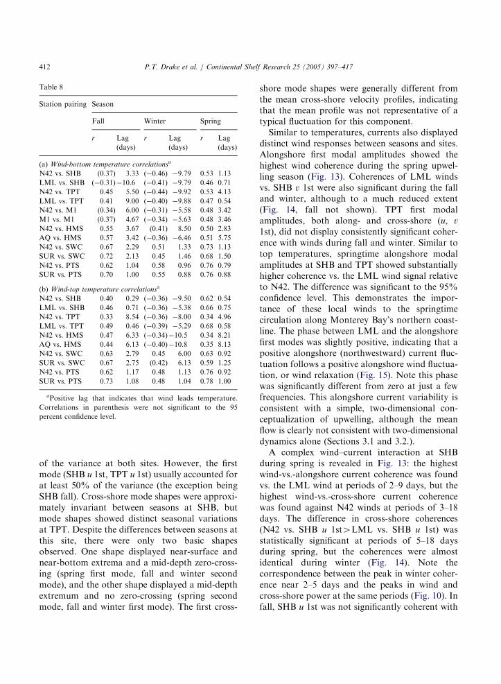
tion of the two variables, showed distinct differ-ences both between seasons and sites. Maximumlagged correlations were highest during fall andspring (Tables 8a and b), and highest at the twosouthernmost sites outside Monterey Bay, SWCand PTS. These sites also had the coldest meansduring spring and fall. Except for TPT toptemperature, wind–temperature correlations didnot improve relative to N42 by using winds from astation closer to a given temperature mooring. Thenegative correlations found during winter at largelags (76–10 days) for stations SHB, TPT, M1 andHMS were not statistically significant and were theresult of the proportionately high long-periodvariance in the temperature records at these sites.These records were almost sinusoidal with a periodof �40–60 days, resulting in few effective degreesof freedom and relatively high, periodic correla-tions at large lags, both positive and negative.Bottom and top temperatures at the two north-ernmost sites (SHB and TPT), as well as M1’s 10mtemperature, were most correlated with windsduring spring. Wind correlations were slightlyhigher for top temperatures than for bottomtemperatures at SHB and TPT during this season,and correlations were highest vs. LML winds.HMS temperatures, however, both top andbottom, showed the strongest wind responseduring fall. At this site wind correlations werehighest with the bottom rather than the toptemperature. Compared to the other sites, SWCand PTS wind–temperature correlations wererelatively high during all three seasons, with thelowest—but still significant—values found inwinter. These fall/spring and top/bottom differ-ences in correlations were, in most cases, notsignificant to the 95% confidence level.Note the relatively long lags displayed by the

HMS top temperature with respect to windsduring fall and spring. This sensor can be seen tobe noticeably out of phase with the bottom sensorduring fall (Fig. 2), an apparent feature of mixedlayer dynamics. In general, HMS showed the leastintra-mooring bottom-vs.-top temperature coher-ence of all the inner shelf sites. SWC and PTSshowed the tightest intra-mooring relation be-tween bottom and top temperatures, with signifi-cant coherence extending from periods of 3–60

ARTICLE IN PRESS

Fig. 7. Wind vs. temperature coherence for bottom temperatures at all inner shelf moorings and M1 10m depth. Horizontal line is the

value where coherence becomes statistically different from zero. At most sites and frequencies with significant coherence, the phase was

positive and significant, indicating that temperatures lag the wind.


days (not shown), and almost complete coherence(g2 � 0:95) between 10 and 60 days. At most sites,where bottom-vs.-top temperature coherence wassignificant, the phase was not significantly differ-ent from zero, indicating that the bottom and toptemperatures fluctuate in-phase. HMS was theexception, with top temperatures lagging bottomtemperatures at long periods and a confused phaserelationship at short periods. The near-zero phaserelationship between bottom and top temperaturesat most sites argues that the correlations of windsand top temperatures (Table 8b) are not artifactsof wind-induced near-surface mixing, but arepredominantly the result of advection (verticaland/or horizontal) of cold, upwelled waterthroughout the water column.

Although something of an anomalous windstation, LML strongly influenced temperaturesand currents (Section 3.6) in its immediate area.This influence on temperature can best be seen byexamining the coherence of winds vs. top tem-

peratures during spring (Fig. 9). Note the highcoherence of SHB and TPT temperatures withLML’s wind signal relative to N42’s. Thedifference was significant at both sites, but thefeature was limited to the spring season. Thiscontrasts with Fig. 7, the same calculationmade over a full year, where there was littledifference in response to the two wind signals. Theaveraging over seasons inherent in the annualcalculation masked the feature. Springtime bottomtemperatures at SHB and TPT displayed the samepattern (high coherence vs. LML, low vs. N42) atperiods of 2–9 days, and were not significantlycoherent with either wind station at 18 days. Ingeneral, seasonal patterns in wind–temperaturecoherence were similar to the patterns in thewind–temperature correlations discussed above:coherences were highest with SWC and PTSduring fall and spring, with the exception of thehigh springtime coherences found with LMLwinds at SHB and TPT.

ARTICLE IN PRESS

Fig. 8. Time history plot of TPT top temperature and LML

alongshore wind (top panel) during spring, showing strong

positive correlation, r ¼ 0.68, between winds and temperature.

Maximum correlation was found when TPT top lagged LML

wind by 14 hours. Bottom panel shows that PTS top

temperature is well-correlated with N42 winds, r ¼ 0.76, with

temperatures lagging winds by 22 h. Monthly tick marks fall on

the first of the month.


3.6. Velocity fluctuations and their associated wind

forcing

Current velocities also displayed a strongresponse to the wind, especially during spring,although there were substantial differences withthe wind/temperature behavior. Near-surface ve-locity spectra (Fig. 10) showed proportionatelymuch less low-frequency power than temperaturespectra. Alongshore velocity spectra at both SHBand TPT were roughly similar to N42’s spectraduring spring, displaying one broad band of powerbetween 3 and 25 days. Relative to alongshorevelocities, cross-shore velocities showed proportio-nately more variance at higher frequencies: Notethe fairly well-defined peak in SHB cross-shorepower near 3.5 days during winter and spring.Near-bottom velocities showed similar spectra(not shown) to near-surface currents, althoughthe absolute power was much reduced in thealongshore component.

It was found that the velocity fluctuations werebest described with an empirical orthogonaldecomposition (Kundu et al., 1975), as just twoempirical orthogonal functions, or EOFs, coulddescribe most of the variance in either velocitycomponent. The EOF decomposition is a statis-tical treatment requiring no dynamical assump-tions. It reduces the data into spatial (in this case,vertical) modes, each with its own time-dependentamplitude. The data can be reproduced as a linearcombination of the modes, each mode modulatedby its respective time-dependent amplitude. Thistreatment also has the advantages that the modesare orthogonal in space, uncorrelated in time, andeach mode’s contribution to the overall variance isreadily calculated. In the decomposition, thevelocity components were treated separately asscalars.The largest two mode shapes at SHB and TPT

for both the alongshore (v) and cross-shore (u)velocity for each season are shown in Figs. 11 and12. The percent variance explained, or overallcontribution of each mode to the variance of itsrespective velocity component, is also given inTable 9. The first alongshore mode (SHB v 1st,TPT v 1st) represented vast bulk (84–97%) of thealongshore variance at both sites. As the along-shore variance dwarfs the cross-shore variance(Fig. 10), these modes also represented the bulk ofthe total current variance (½

PvarðuÞ

PþvarðvÞ;

where the sum is over the water depth). At bothsites, the two largest alongshore modes wereremarkably invariant between seasons. The rela-tively noisy shape of the alongshore second modeat SHB during fall can be attributed to the whitenoise used to fill a 16-day gap in August of 2001(Fig. 2). The alongshore first mode lacked a zero-crossing at both sites and was similar to the meanalongshore velocity profiles found during fall andspring (Fig. 4). This was particularly true at TPT,indicating that the shape of the mean alongshorevelocity profile was also representative of thefluctuations during these seasons. In anothersimilarity to the mean profiles, the alongshore firstmode at TPT displayed slightly more shear relativeto SHB during fall and spring.Unlike the alongshore modes, the cross-shore

second modes each represented a sizable fraction

ARTICLE IN PRESS

Table 8

Station pairing Season

Fall Winter Spring

r Lag

(days)

r Lag

(days)

r Lag

(days)

(a) Wind-bottom temperature correlationsa

N42 vs. SHB (0.37) 3.33 (�0.46) �9.79 0.53 1.13

LML vs. SHB (�0.31)�10.6 (�0.41) �9.79 0.46 0.71

N42 vs. TPT 0.45 5.50 (�0.44) �9.92 0.53 4.13

LML vs. TPT 0.41 9.00 (�0.40) �9.88 0.47 0.54

N42 vs. M1 (0.34) 6.00 (�0.31) �5.58 0.48 3.42

M1 vs. M1 (0.37) 4.67 (�0.34) �5.63 0.48 3.46

N42 vs. HMS 0.55 3.67 (0.41) 8.50 0.50 2.83

AQ vs. HMS 0.57 3.42 (�0.36) �6.46 0.51 5.75

N42 vs. SWC 0.67 2.29 0.51 1.33 0.73 1.13

SUR vs. SWC 0.72 2.13 0.45 1.46 0.68 1.50

N42 vs. PTS 0.62 1.04 0.58 0.96 0.76 0.79

SUR vs. PTS 0.70 1.00 0.55 0.88 0.76 0.88

(b) Wind-top temperature correlationsa

N42 vs. SHB 0.40 0.29 (�0.36) �9.50 0.62 0.54

LML vs. SHB 0.46 0.71 (�0.36) �5.38 0.66 0.75

N42 vs. TPT 0.33 8.54 (�0.36) �8.00 0.34 4.96

LML vs. TPT 0.49 0.46 (�0.39) �5.29 0.68 0.58

N42 vs. HMS 0.47 6.33 (�0.34)�10.5 0.34 8.21

AQ vs. HMS 0.44 6.13 (�0.40)�10.8 0.35 8.13

N42 vs. SWC 0.63 2.79 0.45 6.00 0.63 0.92

SUR vs. SWC 0.67 2.75 (0.42) 6.13 0.59 1.25

N42 vs. PTS 0.62 1.17 0.48 1.13 0.76 0.92

SUR vs. PTS 0.73 1.08 0.48 1.04 0.78 1.00

aPositive lag that indicates that wind leads temperature.

Correlations in parenthesis were not significant to the 95

percent confidence level.


of the variance at both sites. However, the firstmode (SHB u 1st, TPT u 1st) usually accounted forat least 50% of the variance (the exception beingSHB fall). Cross-shore mode shapes were approxi-mately invariant between seasons at SHB, butmode shapes showed distinct seasonal variationsat TPT. Despite the differences between seasons atthis site, there were only two basic shapesobserved. One shape displayed near-surface andnear-bottom extrema and a mid-depth zero-cross-ing (spring first mode, fall and winter secondmode), and the other shape displayed a mid-depthextremum and no zero-crossing (spring secondmode, fall and winter first mode). The first cross-

shore mode shapes were generally different fromthe mean cross-shore velocity profiles, indicatingthat the mean profile was not representative of atypical fluctuation for this component.Similar to temperatures, currents also displayed

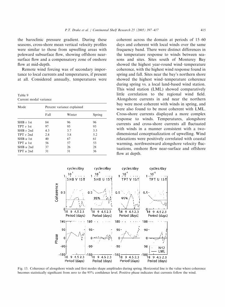
distinct wind responses between seasons and sites.Alongshore first modal amplitudes showed thehighest wind coherence during the spring upwel-ling season (Fig. 13). Coherences of LML windsvs. SHB v 1st were also significant during the falland winter, although to a much reduced extent(Fig. 14, fall not shown). TPT first modalamplitudes, both along- and cross-shore (u, v

1st), did not display consistently significant coher-ence with winds during fall and winter. Similar totop temperatures, springtime alongshore modalamplitudes at SHB and TPT showed substantiallyhigher coherence vs. the LML wind signal relativeto N42. The difference was significant to the 95%confidence level. This demonstrates the impor-tance of these local winds to the springtimecirculation along Monterey Bay’s northern coast-line. The phase between LML and the alongshorefirst modes was slightly positive, indicating that apositive alongshore (northwestward) current fluc-tuation follows a positive alongshore wind fluctua-tion, or wind relaxation (Fig. 15). Note this phasewas significantly different from zero at just a fewfrequencies. This alongshore current variability isconsistent with a simple, two-dimensional con-ceptualization of upwelling, although the meanflow is clearly not consistent with two-dimensionaldynamics alone (Sections 3.1 and 3.2.).A complex wind–current interaction at SHB

during spring is revealed in Fig. 13: the highestwind-vs.-alongshore current coherence was foundvs. the LML wind at periods of 2–9 days, but thehighest wind-vs.-cross-shore current coherencewas found against N42 winds at periods of 3–18days. The difference in cross-shore coherences(N42 vs. SHB u 1st4LML vs. SHB u 1st) wasstatistically significant at periods of 5–18 daysduring spring, but the coherences were almostidentical during winter (Fig. 14). Note thecorrespondence between the peak in winter coher-ence near 2–5 days and the peaks in wind andcross-shore power at the same periods (Fig. 10). Infall, SHB u 1st was not significantly coherent with

ARTICLE IN PRESS

Fig. 9. Springtime wind vs. top temperature coherence, as in Fig. 7, but for springtime top temperatures.


LML winds, but did show significant coherencewith N42 at periods of 9–18 days (not shown). TheTPT cross-shore first mode was only significantlycoherent with winds during spring and showed itshighest coherence with LML. The phase betweenwinds and cross-shore modes was slightly positivein spring and both positive and negative in winter,depending on the wind–current pairing, but wasnowhere significantly different from zero. Thecoherence, phasing, vertical structure and relativesize of the mode shapes indicate a straightforwardcross-shore wind response: Positive (northwest-ward) wind fluctuations induce onshore currentfluctuations near-surface and offshore fluctuationsnear-bottom, with no significant lag (Fig. 15).Conversely, southward (upwelling favorable) windfluctuations result in offshore fluctuations near-surface and onshore flow near-bottom. This isagain consistent with a classical picture of upwel-ling and Ekman dynamics, with equatorward

winds driving offshore flow in the surface layer,resulting in compensatory onshore flow at depth.At SHB, cross-shore currents exhibited thispattern all three seasons, but at TPT the processwas limited to spring.

4. Summary

During 2001 and 2002, inner shelf temperaturesin the Monterey Bay area showed an annual cycleand general seasonality consistent with earlierobservations from within Monterey Bay (Grahamand Largier, 1997) and mid-shelf observationsfrom the central and northern California coast(Largier et al., 1993; Strub et al., 1987). Theseasonal wind behavior, measured at numerousstations, was also consistent with previous mea-surements (Halliwell and Allen, 1987). However,the annual cycle of inner shelf currents near the

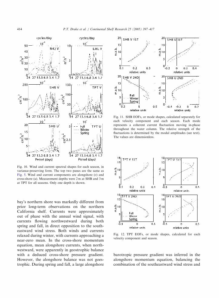
ARTICLE IN PRESS

Fig. 10. Wind and current spectral shapes for each season, in

variance-preserving form. The top two panes are the same as

Fig. 5. Wind and current components are alongshore (v) and

cross-shore (u). Measurement depths were 2m at SHB and 3m

at TPT for all seasons. Only one depth is shown.

Fig. 11. SHB EOFs, or mode shapes, calculated separately for

each velocity component and each season. Each mode

represents a coherent current fluctuation moving in-phase

throughout the water column. The relative strength of the

fluctuations is determined by the modal amplitudes (see text).

The values are dimensionless.

Fig. 12. TPT EOFs, or mode shapes, calculated for each

velocity component and season.


bay’s northern shore was markedly different fromprior long-term observations on the northernCalifornia shelf. Currents were approximatelyout of phase with the annual wind signal, withcurrents flowing northwestward during bothspring and fall, in direct opposition to the south-eastward wind stress. Both winds and currentsrelaxed during winter, with currents approaching anear-zero mean. In the cross-shore momentumequation, mean alongshore currents, when north-westward, were apparently in geostrophic balancewith a deduced cross-shore pressure gradient.However, the alongshore balance was not goes-trophic. During spring and fall, a large alongshore

barotropic pressure gradient was inferred in thealongshore momentum equation, balancing thecombination of the southeastward wind stress and

ARTICLE IN PRESS


the baroclinic pressure gradient. During theseseasons, cross-shore mean vertical velocity profileswere similar to those from upwelling areas withpoleward subsurface flow, showing offshore near-surface flow and a compensatory zone of onshoreflow at mid-depth.

Remote wind forcing was of secondary impor-tance to local currents and temperatures, if presentat all. Considered annually, temperatures were

Table 9

Current modal variance

Mode Percent variance explained

Fall Winter Spring

SHB v 1st 84 96 96

TPT v 1st 97 95 93

SHB v 2nd 4.3 3.7 3.5

TPT v 2nd 2.8 3.8 5.2

SHB u 1st 40 67 61

TPT u 1st 56 57 53

SHB u 2nd 37 26 28

TPT u 2nd 31 31 36

Fig. 13. Coherence of alongshore winds and first modes shape amplit

becomes statistically significant from zero to the 95% confidence leve

coherent across the domain at periods of 15–60days and coherent with local winds over the samefrequency band. There were distinct differences inthe temperature response to winds between sea-sons and sites. Sites south of Monterey Bayshowed the highest year-round wind–temperaturecoherence, with the highest wind response found inspring and fall. Sites near the bay’s northern shoreshowed the highest wind–temperature coherenceduring spring vs. a local land-based wind station.This wind station (LML) showed comparativelylittle correlation to the regional wind field.Alongshore currents in and near the northernbay were most coherent with winds in spring, andwere also found to be most coherent with LML.Cross-shore currents displayed a more complexresponse to winds. Temperatures, alongshorecurrents and cross-shore currents all fluctuatedwith winds in a manner consistent with a two-dimensional conceptualization of upwelling. Windrelaxations were positively correlated with coastalwarming, northwestward alongshore velocity fluc-tuations, onshore flow near-surface and offshoreflow at depth.

udes during spring. Horizontal line is the value where coherence

l. Positive phase indicates that currents follow the wind.

ARTICLE IN PRESS

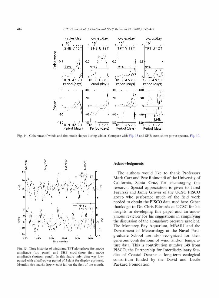
Fig. 14. Coherence of winds and first mode shapes during winter. Compare with Fig. 13 and SHB cross-shore power spectra, Fig. 10.

Fig. 15. Time histories of winds and TPT alongshore first mode

amplitude (top panel) and SHB cross-shore first mode

amplitude (bottom panel). In this figure only, data was low-

passed with a half-power period of 3 days for display purposes.

Monthly tick marks (top x-axis) fall on the first of the month.


Acknowledgments

The authors would like to thank ProfessorsMark Carr and Pete Raimondi of the University ofCalifornia, Santa Cruz, for encouraging thisresearch. Special appreciation is given to JaredFigurski and Jamie Grover of the UCSC PISCOgroup who performed much of the field workneeded to obtain the PISCO data used here. Otherthanks go to Dr. Chris Edwards at UCSC for hisinsights in developing this paper and an anon-ymous reviewer for his suggestions in simplifyingthe discussion of the alongshore pressure gradient.The Monterey Bay Aquarium, MBARI and theDepartment of Meteorology at the Naval Post-graduate School are also recognized for theirgenerous contributions of wind and/or tempera-ture data. This is contribution number 149 fromPISCO, the Partnership for Interdisciplinary Stu-dies of Coastal Oceans: a long-term ecologicalconsortium funded by the David and LucilePackard Foundation.

ARTICLE IN PRESS


References

Allen, J.S., 1975. Coastal trapped waves in a stratified ocean.

Journal of Physical Oceanography 5, 300–325.

Bendat, J.S., Piersol, A.G., 2000. Random Data. Wiley, New

York (594pp).

Breaker, L.C., Broenkow, W.W., 1994. The circulation of

Monterey Bay and related processes. Oceanography and

Marine Biology: An Annual Review 32, 1–64.

Chelton, D.B., Bratkovich, A.W., Bernstein, R.L., Kosro,

P.M., 1988. Poleward flow off central California during the

spring and summer of 1981 and 1984. Journal of Geophy-

sical Research 93 (C9), 10,604–10,620.

Davis, R.E., Bogden, P.S., 1989. Variability on the California

shelf forced by local and remote winds during the coastal

ocean dynamics experiment. Journal of Geophysical Re-

search 94 (C4), 4763–4783.

Denbo, D.W., Allen, J.S., 1987. Large-scale response to

atmospheric forcing of shelf currents and coastal sea level

off the West Coast of North America: May–July 1981 and

1982. Journal of Geophysical Research 92 (C2), 1757–1782.

Emery, W.J., Thomson, R.E., 1997. Data Analysis Methods in

Physical Oceanography. Elsevier, New York (634pp).

Graham, W.M., Largier, J.L., 1997. Upwelling shadows as

nearshore retention sites: the example of northern Monterey

Bay. Continental Shelf Research 17 (5), 509–532.

Halliwell Jr., G.R., Allen, J.S., 1987. The large-scale coastal

wind field along the West Coast of North America,

1981–1982. Journal of Geophysical Research 92 (C2),

1861–1884.

Harris, F.J., 1978. On the use of windows for harmonic analysis

with the discrete Fourier transform. Proceedings of the

IEEE 66, 51–83.

Huyer, A., 1983. Coastal upwelling in the California current

system. Progress in Oceanography 12, 259–284.

Kosro, P.M., Huyer, A., Ramp, S.R., Smith, R.L., Chavez,

F.P., Cowles, T.J., Abbott, M.R., Strub, P.T., Barber, R.T.,

Jessen, P., Small, L.F., 1991. The structure of the transition

zone between coastal waters and the open ocean off

Northern California, winter and spring 1987. Journal of

Geophysical Research 96 (C8), 14,707–14,730.

Kundu, P.K., Allen, J.S., 1976. Some three-dimensional

characteristics of low-frequency current fluctuations near

the Oregon Coast. Journal of Physical Oceanography 6,

181–199.

Kundu, P.K., Allen, J.S., Smith, R.L., 1975. Modal decom-

position of the velocity field near the Oregon Coast. Journal

of Physical Oceanography 5, 683–704.

Large, W.G., Pond, S., 1981. Open ocean momentum flux

measurements in moderate to strong winds. Journal of

Physical Oceanography 11, 324–336.

Largier, J.L., Magnell, B.A., Winant, C.D., 1993. Subtidal

circulation over the Northern California Shelf. Journal of

Geophysical Research 98 (C10), 18,147–18,179.

Lentz, S.J., 1987. A description of the 1981 and 1982 spring

transitions over the Northern California Shelf. Journal of

Geophysical Research 92 (C2), 1545–1567.

Lentz, S.J., 1994. Current dynamics over the Northern

California Shelf. Journal of Physical Oceanography 24,

2461–2478.

Lentz, S., Trowbridge, J., 2001. A dynamical description of fall

and winter mean current profiles over the Northern

California Shelf. Journal of Physical Oceanography 31,

914–931.

Paduan, J.D., Rosenfeld, L.K., 1996. Remotely sensed surface

currents in Monterey Bay from shore-based HF radar

(Coastal Ocean Dynamics Radar). Journal of Geophysical

Research 101 (C9), 20,669–20,686.

Pringle, P.M., Riser, K., 2003. Remotely forced nearshore

upwelling in Southern California. Journal of Geophysical

Research 108 (C4), 3131.

Ramp, S.R., Abbott, C.L., 1998. The vertical structure of

currents over the Continental Shelf off point Sur, CA,

during spring 1990. Deep Sea Research II 45, 1443–1470.

Smith, R.L., 1981. A comparison of the structure and

variability of the flow field in three coastal upwelling

regions: Oregon, Northwest Africa, and Peru. In: Richards,

F.A. (Ed.), Coastal Upwelling, Coastal and Estuarine

Science, vol. 1. AGU, Washington, DC, pp. 107–118.

Storlazzi, C.D., McManus, M.A., Figurski, J.D., 2003. Long-

term, high-frequency current and temperature measure-

ments along central California: insights into upwelling/

relaxation and internal waves on the inner shelf. Continental

Shelf Research 23 (9), 901–918.

Strub, P.T., Allen, J.S., Huyer, A., Smith, R.L., 1987.

Seasonal cycles of currents, temperatures, winds, and

sea level over the Northeast Pacific Continental Shelf:

351N to 481N. Journal of Geophysical Research 92 (C2),

1507–1526.

Thompson, R.O.R.Y., 1979. Coherence significance levels.

Journal of the Atmospheric Sciences 36, 2020–2021.

Winant, C.D., Beardsley, R.C., Davis, R.E., 1987. Moored

wind, temperature, and current observations made during

coastal ocean dynamics experiments 1 and 2 Over Northern

California continental shelf and upper slope. Journal of

Geophysical Research 92 (C2), 1569–1604.

Local wind forcing of the Monterey Bay area inner shelf

Documents

Transcript of Local wind forcing of the Monterey Bay area inner shelf