FIRE FIGHTING TACTICS UNDER WIND DRIVEN CONDITIONS
417
NIST Technical Note 1618 Fire Fighting Tactics Under Wind Driven Conditions: Laboratory Experiments Daniel Madrzykowski Stephen Kerber U.S. Department of Commerce Building and Fire Research Laboratory National Institute of Standards and Technology Gaithersburg, MD 20899 January 2009
-
Upload
khangminh22 -
Category
Documents
-
view
3 -
download
0
Transcript of FIRE FIGHTING TACTICS UNDER WIND DRIVEN CONDITIONS

NIST Technical Note 1618
Fire Fighting Tactics Under Wind Driven Conditions: Laboratory Experiments
Daniel Madrzykowski Stephen Kerber
U.S. Department of Commerce Building and Fire Research Laboratory
National Institute of Standards and Technology Gaithersburg, MD 20899
January 2009


NIST Technical Note 1618 Fire Fighting Tactics Under Wind Driven Conditions: Laboratory Experiments
Daniel Madrzykowski Stephen Kerber
U.S. Department of Commerce Building and Fire Research Laboratory
National Institute of Standards and Technology Gaithersburg, MD 20899
January 2009
Department of Homeland Security Janet Napolitano, Secretary Federal Emergency Management Association, Nancy Ward, Acting Administrator United States Fire Administration Denis Onieal, Acting Administrator
U.S. Department of Commerce Otto J. Wolff, Acting Secretary
National Institute of Standards and Technology
Patrick D. Gallagher, Deputy Director


i
Abstract The National Institute of Standards and Technology, with the support of the Fire Protection Research Foundation and the U.S. Fire Administration conducted eight fire experiments to examine the impact of wind on fire spread through a multi-room structure and examine the capabilities of wind-control devices (WCD) and externally applied water to mitigate the hazard. The measurements used to examine the impact of the WCDs and the external water application tactics were heat release rate, temperature, heat flux, and gas velocity inside the structure. Measurements of oxygen, carbon dioxide, carbon monoxide, total hydrocarbons and differential pressures were also measured. Each of the experiments was recorded with video and thermal imaging cameras. The experiments were designed to expose a public corridor area to a wind driven, post-flashover apartment fire. The door from the apartment to the corridor was open for each of the experiments. The conditions in the corridor were of critical importance because that is the portion of the building that firefighters would use to approach the fire apartment or that occupants from an adjoining apartment would use to exit the building. The fires were ignited in the bedroom of the apartment. Prior to the failure or venting of the bedroom window, which was on the upwind side of the experimental apartment, the heat realease rate from the fire was on the order of 1 MW. Prior to implementing either of the mitigating tactics, the heat release rates from the post-flashover structure fire were typically between 15 MW and 20 MW. When the door from the apartment to the corridor was open, temperatures in the corridor area near the open doorway, 1.52 m (5.00 ft) below the ceiling, were in excess of 600 °C (1112 °F) for each of the experiments. The heat fluxes measured in the same location, during the same experiments, were in excess of 70 kW/m². These extreme thermal conditions are not teneable, even for a firefighter in fully protective gear. These conditions were attained within 30 s of the window failure. In these experiments, the WCDs reduced the temperatures in the corridor outside the doorway by more than 50 % within 60 s of deployment. The heat fluxes were reduced by at least 70 % during this same time period. The WCDs also mitigated completely any gas velocity due to the external wind. The externally applied water streams were implemented in three different ways; a fog stream across the face of the window opening, a fog stream into the window opening, and a solid water stream into the window opening. The fog stream across the window was not effective at reducing the thermal conditions in the corridor. The fog stream in the window decreased the corridor temperature by at least 20 % and the corresponding heat flux measures by at least 30 %. The solid streams experiments resulted in corridor temperature and heat flux reductions of at least 40 % within 60 s of application. None of the water applications had a significant impact on reducing the gas velocities in the structure. In some cases the gas velocity increased during water application. These experiments demonstrated the thermal conditions that can be generated by a “simple room and contents” fire and how these conditions can be extended along a flow path within a structure when a wind condition and an open vent are present. Two potential tactics which could be implemented from either the floor above the fire in the case of a WCD or from the floor below the fire in the case of the external water application were demonstrated to be effective in reducing the thermal hazard in the corridor. Other data and observations, such as the fire pulsing out of the window opening against the wind, can provide valuable information to the fire service for hazard recognition purposes. Further research in an actual building is required to fully understand the ability of firefighters to implement these tactics, to examine the thermal condition through the structure such as in stairways, and to examine the interaction of these tactics with building ventilation strategies both natural and with positive pressure ventilation. This report also includes a series of heat release rate experiments which were used to characterize the fuel packages for these and future experiments.

ii
Disclaimer
Certain trade names or company products are mentioned in the text to specify adequately the experimental procedure and equipment used. In no case does such identification imply recommendation or endorsement by the National Institute of Standards and Technology, nor does it imply that the equipment is the best available for the purpose. Regarding Non-Metric Units: The policy of the National Institute of Standards and Technology is to use metric units in all its published materials. To aid the understanding of this report, in most cases, measurements are reported in both metric and U.S. customary units.

iii
Acknowledgements The authors would like to express their appreciation to the many Building and Fire Research staff members, who provided their technical expertise to make these experiments a success, especially Roy McLane, Jay McElroy, Jonathan Kent, Laurean DeLauter, Anthony Chakalis, Greg Masenheimer, Doris Rinehart, Matt Bundy, Nelson Bryner, J. Randall Lawson, John Wamsley and Luis Luyo. We would also like to thank Anthony Hamins and Rodney Bryant for their thorough review of this document. NIST would like to thank the Montgomery County Fire and Rescue Service for their support of this project, especially the use of the Yankee Air Boat, from the Cabin John Park Volunteer Fire Department and especially Larry Simmons for his skill and consistency is controlling the motor speed of the air boat to provide a consistent “wind” for the experiments and Donald Simmons for his efforts in co-ordinating the experiment schedules with the availability of staff and equipment. We would also like to thank Rick Merck, Tyler Mosman and Patsy Warnick of the Montgomery County Fire Marshal’s Office for their assistance in mapping the NIST Large Fire Facility. We would like to thank Casey Grant, Kathleen Almand and Tracy Golinveaux of the Fire Protection Research Foundation and Meredith Lawler of the U.S. Fire Administration and the DHS Assistance to Firefighters Research and Development Grant Program staff for their support of this project. Finally we would like to thank the members of the project panel for their passion for firefighter safety and expertise especially; Brett Bowman, Prince William County Fire & Rescue, Fairfax VA (IAFC SHS Section Rep); John (Skip) Coleman, Toledo FRD, Toledo, OH; Kevin Courtney, Star FD, Star ID (NVFC Rep); Rich Duffy (IAFF); Richard Edgeworth, Chicago FD, Chicago, IL; Wei Gao (China Fire Protection Association); George Healey, FDNY, New York; Mark Huff, Phoenix FD, Phoenix, AZ; Carl Matejka, Houston FD, Houston TX; Peter McBride, Ottawa FD, Ottawa ON Canada; Jim Milke, University of Maryland (NFPA TC on Smoke Management); John Miller, LA City FD, Los Angeles CA (HRB-SAC Rep); Jack Mooney, FDNY, New York; Carl Peterson, NFPA (NFPA 1500 TC Staff Liaison); Gerald Tracy, FDNY, New York NY, Peter Vandorpe, Chicago FD, Chicago IL; Rick Verlinda, Seattle FD, Seattle WA; Phil Welch, Gaston College, Dallas NC (NFPA Training TC rep); and Michael Wieder, OSU Fire Publications, Stillwater OK, (IFSTA).

iv

v
Table of Contents Abstract .................................................................................................................................................. i Disclaimer ............................................................................................................................................. ii Acknowledgements.............................................................................................................................. iii Table of Contents.................................................................................................................................. v List of Figures .................................................................................................................................... viii List of Tables .................................................................................................................................... xxii 1 Introduction................................................................................................................................... 1
1.1 Background........................................................................................................................... 1 1.1.1 Historical Wind Driven Fires........................................................................................ 2 1.1.2 Experience of the Fire Department of New York City ................................................. 2 1.1.3 U.S. Wind Driven Fire Experience ............................................................................... 4 1.1.4 NFPA Wind Driven Analysis ....................................................................................... 4 1.1.5 Wind Driven Tactics Research ..................................................................................... 4
2 Technical Approach ...................................................................................................................... 6 2.1 Objectives ............................................................................................................................. 6 2.2 Experiments .......................................................................................................................... 7
3 Heat Release Rate Experiments .................................................................................................... 7 3.1 Instrumentation and Uncertainty........................................................................................... 7 3.2 Trash Container Fuel Package .............................................................................................. 9 3.3 Bed Fuel Package................................................................................................................ 14
3.3.1 Bed Fuel Package 1..................................................................................................... 16 3.3.2 Bed Fuel Package 2..................................................................................................... 20
3.4 Upholstered Chair ............................................................................................................... 24 3.4.1 Upholstered Chair 1 .................................................................................................... 25 3.4.2 Upholstered Chair 2 .................................................................................................... 30
3.5 Sleeper Sofa Fuel Package.................................................................................................. 34 3.6 Discussion - Heat Release Rate Experiment Results.......................................................... 40
4 Experimental Arrangement......................................................................................................... 41 4.1 Facility ................................................................................................................................ 41
4.1.1 Structure...................................................................................................................... 41 4.1.2 Instrumentation ........................................................................................................... 46 4.1.3 Estimated Measurement Uncertainty.......................................................................... 47
4.2 Fuel Load ............................................................................................................................ 51 4.3 Wind Source........................................................................................................................ 56
4.3.1 Wind Speed and Pressure Experiments ...................................................................... 56 4.3.2 Wind Control Device Experiments............................................................................. 58 4.3.3 Water Spray Distribution Experiments....................................................................... 60
5 Structure Fire Experiments ......................................................................................................... 64 5.1 Baseline Experiment WDF 1 .............................................................................................. 66
5.1.1 Observations ............................................................................................................... 66 5.1.2 Heat Release Rate ....................................................................................................... 80 5.1.3 Temperatures............................................................................................................... 80 5.1.4 Heat Flux..................................................................................................................... 89 5.1.5 Pressure ....................................................................................................................... 90

vi
5.1.6 Velocities .................................................................................................................... 90 5.1.7 Gas Concentrations ..................................................................................................... 94
5.2 Wind Control Devices WDF 2............................................................................................ 98 5.2.1 Observations ............................................................................................................... 99 5.2.2 Heat Release Rate ..................................................................................................... 111 5.2.3 Temperatures............................................................................................................. 111 5.2.4 Heat Flux................................................................................................................... 120 5.2.5 Pressure ..................................................................................................................... 121 5.2.6 Velocities .................................................................................................................. 122 5.2.7 Gas Concentrations ................................................................................................... 126
5.3 Wind Control Devices WDF 3.......................................................................................... 129 5.3.1 Observations ............................................................................................................. 129 5.3.2 Heat Release Rate ..................................................................................................... 144 5.3.3 Temperatures............................................................................................................. 145 5.3.4 Heat Flux................................................................................................................... 153 5.3.5 Pressure ..................................................................................................................... 154 5.3.6 Velocities .................................................................................................................. 155 5.3.7 Gas Concentrations ................................................................................................... 159
5.4 Wind Control Devices with suppression WDF 4.............................................................. 162 5.4.1 Observations ............................................................................................................. 162 5.4.2 Heat Release Rate ..................................................................................................... 177 5.4.3 Temperatures............................................................................................................. 177 5.4.4 Heat Flux................................................................................................................... 186 5.4.5 Pressure ..................................................................................................................... 186 5.4.6 Velocities .................................................................................................................. 187 5.4.7 Gas Concentrations ................................................................................................... 191
5.5 Wind Control Devices with suppression WDF 5.............................................................. 194 5.5.1 Observations ............................................................................................................. 194 5.5.2 Heat Release Rate ..................................................................................................... 210 5.5.3 Temperatures............................................................................................................. 210 5.5.4 Heat Flux................................................................................................................... 218 5.5.5 Pressure ..................................................................................................................... 219 5.5.6 Velocities .................................................................................................................. 220 5.5.7 Gas Concentrations ................................................................................................... 224
5.6 External Water Application (indirect attack) WDF 6 (fog) .............................................. 226 5.6.1 Observations ............................................................................................................. 227 5.6.2 Heat Release Rate ..................................................................................................... 245 5.6.3 Temperatures............................................................................................................. 245 5.6.4 Heat Flux................................................................................................................... 258 5.6.5 Pressure ..................................................................................................................... 259 5.6.6 Velocities .................................................................................................................. 260 5.6.7 Gas Concentrations ................................................................................................... 265
5.7 External Water Application (indirect attack) WDF 7 (smooth bore) ............................... 270 5.7.1 Observations ............................................................................................................. 271 5.7.2 Heat Release Rate ..................................................................................................... 286 5.7.3 Temperatures............................................................................................................. 286

vii
5.7.4 Heat Flux................................................................................................................... 294 5.7.5 Pressure ..................................................................................................................... 295 5.7.6 Velocities .................................................................................................................. 296 5.7.7 Gas Concentrations ................................................................................................... 300
5.8 External Water Application (indirect attack) WDF 8 (smooth bore) ............................... 303 5.8.1 Observations ............................................................................................................. 303 5.8.2 Heat Release Rate ..................................................................................................... 320 5.8.3 Temperatures............................................................................................................. 320 5.8.4 Heat Flux................................................................................................................... 327 5.8.5 Pressure ..................................................................................................................... 327 5.8.6 Velocities .................................................................................................................. 328 5.8.7 Gas Concentrations ................................................................................................... 332
6 Discussion................................................................................................................................. 335 6.1 Fire Conditions with no external wind.............................................................................. 335 6.2 Tactics ............................................................................................................................... 339
6.2.1 Wind Control Devices............................................................................................... 339 6.2.2 External Water Application ...................................................................................... 345 6.2.3 Door Control ............................................................................................................. 351
7 Future Research ........................................................................................................................ 352 7.1.1 Full-scale experiments .............................................................................................. 353 7.1.2 Pilot Programs........................................................................................................... 353 7.1.3 Standard Test Methods for equipment...................................................................... 353
8 Summary ................................................................................................................................... 353 9 References................................................................................................................................. 356 Appendix A: Summary of Fire Events Where Wind Did or Could Have Impact Fire Fighting Tactics Appendix B: FPRF Project Technical Panel Roster

viii
List of Figures Figure 3.1-1. Typical heat release rate experimental arrangement, using the bed fuel package, with the heat flux positions labeled. This arrangement was used for all chair, bed, and sofa heat release rate experiments. ................................................................................................................................... 8 Figure 3.2-1. Trash container 1, ignition ........................................................................................... 11 Figure 3.2-2. Trash container 1, 100 s after ignition ......................................................................... 11 Figure 3.2-3. Trash container 1, 200 s after ignition ......................................................................... 11 Figure 3.2-4. Trash container 1, 300 s after ignition ......................................................................... 11 Figure 3.2-5. Trash container 1, 400 s after ignition ......................................................................... 11 Figure 3.2-6. Trash container 1, at peak heat release rate, 406 s after ignition ................................. 11 Figure 3.2-7. Trash container 1, 500 s after ignition ......................................................................... 11 Figure 3.2-8. Trash container 1, 600 s after ignition ......................................................................... 11 Figure 3.2-9. Trash container 2, ignition ........................................................................................... 12 Figure 3.2-10. Trash container 2, 100 s after ignition ....................................................................... 12 Figure 3.2-11. Trash container 2, 200 s after ignition ....................................................................... 12 Figure 3.2-12. Trash container 2, 300 s after ignition ....................................................................... 12 Figure 3.2-13. Trash container 2, at peak heat release rate, 363 s after ignition ............................... 12 Figure 3.2-14. Trash container 2, 400 s after ignition ....................................................................... 12 Figure 3.2-15. Trash container 2, 500 s after ignition ....................................................................... 12 Figure 3.2-16. Trash container 2, 600 s after ignition ....................................................................... 12 Figure 3.2-17. Heat release rate versus time for Trash Container 1 and 2. ....................................... 13 Figure 3.2-18. Heat flux versus time for Trash Container 1 and 2. ................................................... 13 Figure 3.2-19. Mass loss versus time for Trash Containers 1 and 2.................................................. 14 Figure 3.3-1. Top side of box spring.................................................................................................. 15 Figure 3.3-2. Bottom side of box spring. ........................................................................................... 15 Figure 3.3-3. Electric match ignition of bed fuel package................................................................. 16 Figure 3.3-4. Trash container ignition of bed fuel package............................................................... 16 Figure 3.3.1-1. Bed 1, ignition........................................................................................................... 17 Figure 3.3.1-2. Bed 1, 100 s after ignition ......................................................................................... 17 Figure 3.3.1-3. Bed 1, 200 s after ignition ......................................................................................... 17 Figure 3.3.1-4. Bed 1, 300 s after ignition ......................................................................................... 17 Figure 3.3.1-5. Bed 1, 400 s after ignition ......................................................................................... 17 Figure 3.3.1-6. Bed 1, at peak heat release rate, 484 s after ignition................................................. 17 Figure 3.3.1-7. Bed 1, 500 s after ignition ......................................................................................... 17 Figure 3.3.1-8. Bed 1, 600 s after ignition ......................................................................................... 17 Figure 3.3.1-9. Bed 1, 700 s after ignition ......................................................................................... 17 Figure 3.3.1-10. Bed 1, 800 s after ignition ....................................................................................... 17 Figure 3.3.1-11. Heat release rate versus time for bed fuel package 1. .............................................. 18 Figure 3.3.1-12. Heat flux versus time for the bed fuel package 1.................................................... 19 Figure 3.3.1-13. Mass loss versus time for bed fuel package 1. ........................................................ 20 Figure 3.3.2-1. Bed 2, ignition........................................................................................................... 21 Figure 3.3.2-2. Bed 2, 100 s after ignition ......................................................................................... 21 Figure 3.3.2-3. Bed 2, 200 s after ignition ......................................................................................... 21 Figure 3.3.2-4. Bed 2, 300 s after ignition ......................................................................................... 21 Figure 3.3.2-5. Bed 2, at peak heat release rate, 380 s after ignition................................................. 21

ix
Figure 3.3.2-6. Bed 2, 400 s after ignition ......................................................................................... 21 Figure 3.3.2-7. Bed 2, 500 s after ignition ......................................................................................... 21 Figure 3.3.2-8. Bed 2, 600 s after ignition ......................................................................................... 21 Figure 3.3.2-9. Heat release rate versus time for bed fuel package 2. ............................................... 22 Figure 3.3.2-10. Heat flux versus time for bed fuel package 2.......................................................... 23 Figure 3.3.2-11. Mass loss versus time for bed fuel package 2. ........................................................ 24 Figure 3.4-1. Upholstered chair, front view....................................................................................... 25 Figure 3.4-2. Upholstered chair, side view. ....................................................................................... 25 Figure 3.4-3. Seat cushion, showing layers of upholstery fabric, polyester batting and polyurethane foam. ................................................................................................................................................... 25 Figure 3.4-4. Back cushion, showing the upholstery fabric, inner liner, and polyurethane foam. .... 25 Figure 3.4.1-1. Chair 1, ignition ........................................................................................................ 27 Figure 3.4.1-2. Chair 1, 100 s after ignition....................................................................................... 27 Figure 3.4.1-3. Chair 1, 200 s after ignition....................................................................................... 27 Figure 3.4.1-4. Chair 1, 300 s after ignition....................................................................................... 27 Figure 3.4.1-5. Chair 1, 400 s after ignition....................................................................................... 27 Figure 3.4.1-6. Chair 1, at peak heat release rate, 417 s after ignition .............................................. 27 Figure 3.4.1-7. Chair 1, 500 s after ignition....................................................................................... 27 Figure 3.4.1-8. Chair 1, 600 s after ignition....................................................................................... 27 Figure 3.4.1-9. Chair 1, 700 s after ignition....................................................................................... 27 Figure 3.4.1-10. Chair 1, 800 s after ignition..................................................................................... 27 Figure 3.4.1-11. Heat release rate versus time for chair 1. ................................................................ 28 Figure 3.4.1-12. Heat flux versus time for chair 1............................................................................. 29 Figure 3.4.1-13. Mass loss versus time for chair 1. ........................................................................... 30 Figure 3.4.2-1. Chair 2, ignition ........................................................................................................ 31 Figure 3.4.2-2. Chair 2, 100 s after ignition....................................................................................... 31 Figure 3.4.2-3. Chair 2, 200 s after ignition....................................................................................... 31 Figure 3.4.2-4. Chair 2, 300 s after ignition....................................................................................... 31 Figure 3.4.2-5. Chair 2, 400 s after ignition....................................................................................... 31 Figure 3.4.2-6. Chair 2, at peak heat release rate, 437 s after ignition .............................................. 31 Figure 3.4.2-7. Chair 2, 500 s after ignition....................................................................................... 31 Figure 3.4.2-8. Chair 2, 600 s after ignition....................................................................................... 31 Figure 3.4.2-9. Chair 2, 700 s after ignition....................................................................................... 31 Figure 3.4.2-10. Chair 2, 800 s after ignition..................................................................................... 31 Figure 3.4.2-11. Heat release rate versus time for chair 2. ................................................................ 32 Figure 3.4.2-12. Heat flux versus time for chair 2............................................................................. 33 Figure 3.4.2-13. Mass loss versus time for chair 2. ........................................................................... 33 Figure 3.5-1. Sofa 1, ignition ............................................................................................................. 35 Figure 3.5-2. Sofa 1, 100 s after ignition ........................................................................................... 35 Figure 3.5-3. Sofa 1, 200 s after ignition ........................................................................................... 35 Figure 3.5-4. Sofa 1, 300 s after ignition ........................................................................................... 35 Figure 3.5-5. Sofa 1, 400 s after ignition ........................................................................................... 35 Figure 3.5-6. Sofa 1, at peak heat release rate, 455 s after ignition................................................... 35 Figure 3.5-7. Sofa 1, 500 s after ignition ........................................................................................... 35 Figure 3.5-8. Sofa 1, 600 s after ignition ........................................................................................... 35 Figure 3.5-9. Sofa 1, 700 s after ignition ........................................................................................... 35

x
Figure 3.5-10. Sofa 1, 800 s after ignition ......................................................................................... 35 Figure 3.5-11. Sofa 2, ignition ........................................................................................................... 36 Figure 3.5-12. Sofa 2, 100 s after ignition ......................................................................................... 36 Figure 3.5-13. Sofa 2, 200 s after ignition ......................................................................................... 36 Figure 3.5-14. Sofa 2, 300 s after ignition ......................................................................................... 36 Figure 3.5-15. Sofa 2, at peak heat release rate, 389 s after ignition................................................. 36 Figure 3.5-16. Sofa 2, 400 s after ignition ......................................................................................... 36 Figure 3.5-17. Sofa 2, 500 s after ignition ......................................................................................... 36 Figure 3.5-18. Sofa 2, 600 s after ignition ......................................................................................... 36 Figure 3.5-19. Sofa 2, 700 s after ignition ......................................................................................... 36 Figure 3.5-20. Sofa 2, 800 s after ignition ......................................................................................... 36 Figure 3.5-21. Heat release rate versus time for sofas 1 and 2. ......................................................... 37 Figure 3.5-22. Heat flux versus time for sofa 1. ................................................................................ 38 Figure 3.5-23. Heat flux versus time for sofa 2. ................................................................................ 38 Figure 3.5-24. Mass loss versus time for sofa 1. ............................................................................... 39 Figure 3.5-25. Mass loss versus time for sofa 2. ............................................................................... 40 Figure 4.1.1-1. Schematic plan view of the experimental structure. ................................................. 42 Figure 4.1.1-2. Steel framing for walls of experimental structure inside the NIST Large Fire Facility. ............................................................................................................................................... 43 Figure 4.1.1-3. Ceiling supports for experimental structure. ............................................................. 44 Figure 4.1.1-4. Dimensioned floor plan of experimental structure.................................................... 45 Figure 4.1.3-1. Schematic floor plan of instrumentation types and locations. .................................. 49 Figure 4.1.3-2. Thermocouple arrays along center line of structure looking from east to west. ....... 50 Figure 4.1.3-3. Bi-directional probe array in west window............................................................... 50 Figure 4.1.3-4. Wall mounted thermocouples, heat flux sensor, and differential pressure sampling port. ..................................................................................................................................................... 50 Figure 4.1.3-5. Gas sampling probe installation on south wall of living room. ................................ 50 Figure 4.2-1. Schematic floor plan of bedroom with furniture locations. ......................................... 52 Figure 4.2-2. Bedroom furnishings, looking north. ........................................................................... 52 Figure 4.2-3. Bedroom furnishings, looking south. ........................................................................... 52 Figure 4.2-4. Schematic floor plan of living room with furniture locations...................................... 54 Figure 4.2-5. Living room furniture, looking north. .......................................................................... 54 Figure 4.2-6. Living room furnishings, looking east. ........................................................................ 54 Figure 4.3-1. Air boat from inside of fire lab looking west. .............................................................. 56 Figure 4.3-2. Air boat from outside of the fire lab looking east. ....................................................... 56 Figure 4.3.2-1. Small WCD deployed over window opening............................................................ 58 Figure 4.3.2-2. Large WCD deployed over window opening............................................................ 58 Figure 4.3.3-1. Water spray distribution experiment arrangement. ................................................... 62 Figure 4.3.3-2. Fog stream discharged across window opening........................................................ 62 Figure 4.3.3-3. Fog stream discharged into window opening............................................................ 62 Figure 4.3.3-4. Solid stream discharged into window opening. ........................................................ 62 Figure 4.3.3-5. Water distribution results for fog stream discharged across window opening (kg), the gray area does not contain a measurable amount of water. ................................................................ 63 Figure 4.3.3-6. Water distribution results for fog stream discharged into window opening (kg), the gray area does not contain a measurable amount of water. ................................................................ 63

xi
Figure 4.3.3-7. Water distribution results for solid stream discharged into window opening (kg), the gray area does not contain a measurable amount of water. ................................................................ 64 Figure 5-1. Photograph of the placement of the trash container fuel package ignition source.......... 65 Figure 5.1.1-1. Experiment 1, ignition............................................................................................... 69 Figure 5.1.1-2. Experiment 1, 60 s after ignition............................................................................... 70 Figure 5.1.1-3. Experiment 1, 120 s after ignition............................................................................. 71 Figure 5.1.1-4. Experiment 1, 180 s after ignition............................................................................. 72 Figure 5.1.1-5. Experiment 1, 240 s after ignition............................................................................. 73 Figure 5.1.1-6. Experiment 1, window fully vented, 260 s after ignition.......................................... 74 Figure 5.1.1-7. Experiment 1, 300 s after ignition............................................................................. 75 Figure 5.1.1-8. Experiment 1, 360 s after ignition............................................................................. 76 Figure 5.1.1-9. Experiment 1, 420 s after ignition............................................................................. 77 Figure 5.1.1-10. Experiment 1, 480 s after ignition........................................................................... 78 Figure 5.1.1-11. Experiment 1, 540 s after ignition........................................................................... 79 Figure 5.1.2-1. Heat release rate versus time, Experiment 1. ............................................................ 80 Figure 5.1.3-1. Temperature versus time from the bedroom window (BRW) thermocouple array, Experiment 1....................................................................................................................................... 83 Figure 5.1.3-2. Temperature versus time from the bedroom (BR) thermocouple array, Experiment 1.............................................................................................................................................................. 84 Figure 5.1.3-3. Temperature versus time from the hall thermocouple array, Experiment 1. ............ 84 Figure 5.1.3-4. Temperature versus time from the living room corner (LRC) thermocouple array, Experiment 1....................................................................................................................................... 85 Figure 5.1.3-5. Temperature versus time from the living room (LR) thermocouple array, Experiment 1........................................................................................................................................................... 85 Figure 5.1.3-6. Temperature versus time from the corridor center (CC) thermocouple array, Experiment 1....................................................................................................................................... 86 Figure 5.1.3-7. Temperature versus time from the corridor south (CS) thermocouple array, Experiment 1....................................................................................................................................... 86 Figure 5.1.3-8. Temperature versus time from the corridor southwest (CSW) thermocouple array, Experiment 1....................................................................................................................................... 87 Figure 5.1.3-9. Temperature versus time from the corridor north (CN) thermocouple array, Experiment 1....................................................................................................................................... 87 Figure 5.1.3-10. Temperature versus time from the ceiling vent thermocouple array, Experiment 1.............................................................................................................................................................. 88 Figure 5.1.3-11. Temperature versus time from the target room (TR) door knobs, Experiment 1. .. 88 Figure 5.1.4-1. Heat flux versus time at five locations, Experiment 1. ............................................. 89 Figure 5.1.5-1. Pressure versus time at five locations, Experiment 1................................................ 90 Figure 5.1.6-1. Velocity versus time from the bedroom window (BRW) bi-directional probe array, Experiment 1....................................................................................................................................... 92 Figure 5.1.6-2. Velocity versus time from the hall bi-directional probe array, Experiment 1. ......... 92 Figure 5.1.6-3. Velocity versus time from the corridor south (CS) bi-directional probe array, Experiment 1....................................................................................................................................... 93 Figure 5.1.6-4. Velocity versus time from the corridor north (CN) bi-directional probe array, Experiment 1....................................................................................................................................... 93 Figure 5.1.6-5. Velocity versus time from the ceiling vent (V) bi-directional probe array, Experiment 1....................................................................................................................................... 94

xii
Figure 5.1.7-1. Oxygen, carbon dioxide, carbon monoxide, and total hydrocarbon percent volume versus time from the upper bedroom (BR) sampling location, Experiment 1. ................................... 96 Figure 5.1.7-2. Oxygen, carbon dioxide, and carbon monoxide percent volume versus time from the lower bedroom (BR) sampling location, Experiment 1. ..................................................................... 96 Figure 5.1.7-3. Oxygen, carbon dioxide, carbon monoxide, and total hydrocarbon percent volume versus time from the upper living (LR) room sampling location, Experiment 1................................ 97 Figure 5.1.7-4. Oxygen, carbon dioxide, and carbon monoxide percent volume versus time from the lower living room (LR) sampling location, Experiment 1.................................................................. 97 Figure 5.1.7-5. Total hydrocarbon percent volumes versus time from the upper bedroom (BR) and living room (LR) sampling locations, Experiment 1. ......................................................................... 98 Figure 5.2.1-1. Experiment 2 ignition.............................................................................................. 101 Figure 5.2.1-2. Experiment 2, 60 s after ignition............................................................................. 102 Figure 5.2.1-3. Experiment 2, 120 s after ignition........................................................................... 103 Figure 5.2.1-4. Experiment 2, 180 s after ignition........................................................................... 104 Figure 5.2.1-5. Experiment 2, corridor flames, 189 s after ignition. ............................................... 105 Figure 5.2.1-6. Experiment 2, WCD deployed; 200 s after ignition................................................ 106 Figure 5.2.1-7. Experiment 2, WCD in place, 205 s after ignition. ................................................. 107 Figure 5.2.1-8. Experiment 2, 240 s after ignition........................................................................... 108 Figure 5.2.1-9. Experiment 2, WCD removed; 270 s after ignition. ............................................... 109 Figure 5.2.1-10. Experiment 2, 300 s after ignition......................................................................... 110 Figure 5.2.2-1. Heat release rate versus time, Experiment 2. .......................................................... 111 Figure 5.2.3-1. Temperature versus time from the bedroom window (BRW) thermocouple array, Experiment 2..................................................................................................................................... 114 Figure 5.2.3-2. Temperature versus time from the bedroom (BR) thermocouple array, Experiment 2............................................................................................................................................................ 115 Figure 5.2.3-3. Temperature versus time from the hall thermocouple array, Experiment 2. .......... 115 Figure 5.2.3-4. Temperature versus time from the living room corner (LRC) thermocouple array, Experiment 2..................................................................................................................................... 116 Figure 5.2.3-5. Temperature versus time from the living room (LR) thermocouple array, Experiment 2......................................................................................................................................................... 116 Figure 5.2.3-6. Temperature versus time from the corridor center (CC) thermocouple array, Experiment 2..................................................................................................................................... 117 Figure 5.2.3-7. Temperature versus time from the corridor south (CS) thermocouple array, Experiment 2..................................................................................................................................... 117 Figure 5.2.3-8. Temperature versus time from the corridor southwest (CSW) thermocouple array, Experiment 2..................................................................................................................................... 118 Figure 5.2.3-9. Temperature versus time from the corridor north (CN) thermocouple array, Experiment 2..................................................................................................................................... 118 Figure 5.2.3-10. Temperature versus time from the ceiling vent thermocouple array, Experiment 2............................................................................................................................................................ 119 Figure 5.2.3-11. Temperature versus time from the target room (TR) door knobs, Experiment 2. 119 Figure 5.2.3-12. Temperature versus time from the target room (TR) thermocouple array, Experiment 2..................................................................................................................................... 120 Figure 5.2.4-1. Heat flux versus time at five locations, Experiment 2. ........................................... 121 Figure 5.2.5-1. Pressure versus time at five locations, Experiment 2.............................................. 122

xiii
Figure 5.2.6-1. Velocity versus time from the bedroom window (BRW) bi-directional probe array, Experiment 2..................................................................................................................................... 123 Figure 5.2.6-2. Velocity versus time from the hall bi-directional probe array, Experiment 2. ....... 124 Figure 5.2.6-3. Velocity versus time from the corridor south (CS) bi-directional probe array, Experiment 2..................................................................................................................................... 124 Figure 5.2.6-4. Velocity versus time from the corridor north (CN) bi-directional probe array, Experiment 2..................................................................................................................................... 125 Figure 5.2.6-5. Velocity versus time from the ceiling vent (V) bi-directional probe array, Experiment 2..................................................................................................................................... 125 Figure 5.2.7-1. Oxygen, carbon dioxide, carbon monoxide, and total hydrocarbon percent volume versus time from the upper bedroom (BR) sampling location, Experiment 2. ................................. 127 Figure 5.2.7-2. Oxygen, carbon dioxide, and carbon monoxide percent volume versus time from the lower bedroom (BR) sampling location, Experiment 2. ................................................................... 127 Figure 5.2.7-3. Oxygen, carbon dioxide, carbon monoxide, and total hydrocarbon percent volume versus time from the upper living (LR) room sampling location, Experiment 2.............................. 128 Figure 5.2.7-4. Oxygen, carbon dioxide, and carbon monoxide percent volume versus time from the lower living room (LR) sampling location, Experiment 2................................................................ 128 Figure 5.3.1-1. Experiment 3, ignition............................................................................................. 132 Figure 5.3.1-2. Experiment 3, 60 s after ignition............................................................................. 133 Figure 5.3.1-3. Experiment 3, 120 s after ignition........................................................................... 134 Figure 5.3.1-4. Experiment 3, 180 s after ignition........................................................................... 135 Figure 5.3.1-5. Experiment 3, window fully vented, 208 s after ignition........................................ 136 Figure 5.3.1-6. Experiment 3, corridor flames, 222 s after ignition. ............................................... 137 Figure 5.3.1-7. Experiment 3, 240 s after ignition........................................................................... 138 Figure 5.3.1-8. Experiment 3, WCD deployed; 266 s after ignition................................................ 139 Figure 5.3.1-9. Experiment 3, WCD in place, 270 s after ignition. ................................................. 140 Figure 5.3.1-10. Experiment 3, 300 s after ignition......................................................................... 141 Figure 5.3.1-11. Experiment 3, WCD removed; 330 s after ignition. ............................................. 142 Figure 5.3.1-12. Experiment 3, 360 s after ignition......................................................................... 143 Figure 5.3.2-1. Heat release rate versus time, Experiment 3. .......................................................... 144 Figure 5.3.3-1. Temperature versus time from the bedroom window (BRW) thermocouple array, Experiment 3..................................................................................................................................... 147 Figure 5.3.3-2. Temperature versus time from the bedroom (BR) thermocouple array, Experiment 3............................................................................................................................................................ 148 Figure 5.3.3-3. Temperature versus time from the hall thermocouple array, Experiment 3. .......... 148 Figure 5.3.3-4. Temperature versus time from the living room corner (LRC) thermocouple array, Experiment 3..................................................................................................................................... 149 Figure 5.3.3-5. Temperature versus time from the living room (LR) thermocouple array, Experiment 3......................................................................................................................................................... 149 Figure 5.3.3-6. Temperature versus time from the corridor center (CC) thermocouple array, Experiment 3..................................................................................................................................... 150 Figure 5.3.3-7. Temperature versus time from the corridor south (CS) thermocouple array, Experiment 3..................................................................................................................................... 150 Figure 5.3.3-8. Temperature versus time from the corridor southwest (CSW) thermocouple array, Experiment 3..................................................................................................................................... 151

xiv
Figure 5.3.3-9. Temperature versus time from the corridor north (CN) thermocouple array, Experiment 3..................................................................................................................................... 151 Figure 5.3.3-10. Temperature versus time from the ceiling vent thermocouple array, Experiment 3............................................................................................................................................................ 152 Figure 5.3.3-11. Temperature versus time from the target room (TR) door knobs, Experiment 3. 152 Figure 5.3.3-12. Temperature versus time from the target room (TR) thermocouple array, Experiment 3..................................................................................................................................... 153 Figure 5.3.4-1. Heat flux versus time at five locations, Experiment 3. ........................................... 154 Figure 5.3.5-1. Pressure versus time at five locations, Experiment 3.............................................. 155 Figure 5.3.6-1. Velocity versus time from the bedroom window (BRW) bi-directional probe array, Experiment 3..................................................................................................................................... 156 Figure 5.3.6-2. Velocity versus time from the hall bi-directional probe array, Experiment 3. ....... 157 Figure 5.3.6-3. Velocity versus time from the corridor south (CS) bi-directional probe array, Experiment 3..................................................................................................................................... 157 Figure 5.3.6-4. Velocity versus time from the corridor north (CN) bi-directional probe array, Experiment 3..................................................................................................................................... 158 Figure 5.3.6-5. Velocity versus time from the ceiling vent (V) bi-directional probe array, Experiment 3..................................................................................................................................... 158 Figure 5.3.7-1. Oxygen, carbon dioxide, carbon monoxide, and total hydrocarbon percent volume versus time from the upper bedroom (BR) sampling location, Experiment 3. ................................. 160 Figure 5.3.7-2. Oxygen, carbon dioxide, and carbon monoxide percent volume versus time from the lower bedroom (BR) sampling location, Experiment 3. ................................................................... 160 Figure 5.3.7-3. Oxygen, carbon dioxide, carbon monoxide, and total hydrocarbon percent volume versus time from the upper living (LR) room sampling location, Experiment 3.............................. 161 Figure 5.3.7-4. Oxygen, carbon dioxide, and carbon monoxide percent volume versus time from the lower living room (LR) sampling location, Experiment 3................................................................ 161 Figure 5.4.1-1. Experiment 4, ignition............................................................................................. 165 Figure 5.4.1-2. Experiment 4, 60 s after ignition............................................................................. 166 Figure 5.4.1-3. Experiment 4, 120 s after ignition........................................................................... 167 Figure 5.4.1-4. Experiment 4, 180 s after ignition........................................................................... 168 Figure 5.4.1-5. Experiment 4, window fully vented, 218 s after ignition........................................ 169 Figure 5.4.1-6. Experiment 4, corridor flames, 234 s after ignition. ............................................... 170 Figure 5.4.1-7. Experiment 4, 240 s after ignition........................................................................... 171 Figure 5.4.1-8. Experiment 4, 268 s after ignition, just prior to WCD deployment. ....................... 172 Figure 5.4.1-9. Experiment 4, WCD in place, 275 s after ignition. ................................................. 173 Figure 5.4.1-10. Experiment 4, 300 s after ignition......................................................................... 174 Figure 5.4.1-11. Experiment 4, 360 s after ignition......................................................................... 175 Figure 5.4.1-12. Experiment 4, 420 s after ignition......................................................................... 176 Figure 5.4.2-1. Heat release rate versus time, Experiment 4. .......................................................... 177 Figure 5.4.3-1. Temperature versus time from the bedroom window (BRW) thermocouple array, Experiment 4..................................................................................................................................... 180 Figure 5.4.3-2. Temperature versus time from the bedroom (BR) thermocouple array, Experiment 4............................................................................................................................................................ 181 Figure 5.4.3-3. Temperature versus time from the hall thermocouple array, Experiment 4. .......... 181 Figure 5.4.3-4. Temperature versus time from the living room corner (LRC) thermocouple array, Experiment 4..................................................................................................................................... 182

xv
Figure 5.4.3-5. Temperature versus time from the living room (LR) thermocouple array, Experiment 4......................................................................................................................................................... 182 Figure 5.4.3-6. Temperature versus time from the corridor center (CC) thermocouple array, Experiment 4..................................................................................................................................... 183 Figure 5.4.3-7. Temperature versus time from the corridor south (CS) thermocouple array, Experiment 4..................................................................................................................................... 183 Figure 5.4.3-8. Temperature versus time from the corridor southwest (CSW) thermocouple array, Experiment 4..................................................................................................................................... 184 Figure 5.4.3-9. Temperature versus time from the corridor north (CN) thermocouple array, Experiment 4..................................................................................................................................... 184 Figure 5.4.3-10. Temperature versus time from the ceiling vent thermocouple array, Experiment 4............................................................................................................................................................ 185 Figure 5.4.3-11. Temperature versus time from the target room (TR) thermocouple array, Experiment 4..................................................................................................................................... 185 Figure 5.4.4-1. Heat flux versus time at five locations, Experiment 4. ........................................... 186 Figure 5.4.5-1. Pressure versus time at five locations, Experiment 4.............................................. 187 Figure 5.4.6-1. Velocity versus time from the bedroom window (BRW) bi-directional probe array, Experiment 4..................................................................................................................................... 189 Figure 5.4.6-2. Velocity versus time from the hall bi-directional probe array, Experiment 4. ....... 189 Figure 5.4.6-3. Velocity versus time from the corridor south (CS) bi-directional probe array, Experiment 4..................................................................................................................................... 190 Figure 5.4.6-4. Velocity versus time from the corridor north (CN) bi-directional probe array, Experiment 4..................................................................................................................................... 190 Figure 5.4.6-5. Velocity versus time from the ceiling vent (V) bi-directional probe array, Experiment 4..................................................................................................................................... 191 Figure 5.4.7-1. Oxygen, carbon dioxide, and carbon monoxide percent volume versus time from the lower bedroom (BR) sampling location, Experiment 4. ................................................................... 192 Figure 5.4.7-2. Oxygen, carbon dioxide, carbon monoxide, and total hydrocarbon percent volume versus time from the upper living (LR) room sampling location, Experiment 4.............................. 193 Figure 5.4.7-3. Oxygen, carbon dioxide, and carbon monoxide percent volume versus time from the lower living room (LR) sampling location, Experiment 4................................................................ 193 Figure 5.5.1-1. Experiment 5, ignition............................................................................................. 197 Figure 5.5.1-2. Experiment 5, 60 s after ignition............................................................................. 198 Figure 5.5.1-3. Experiment 5, 120 s after ignition........................................................................... 199 Figure 5.5.1-4. Experiment 5, 180 s after ignition........................................................................... 200 Figure 5.5.1-5. Experiment 5, 240 s after ignition........................................................................... 201 Figure 5.5.1-6. Experiment 5, corridor flames, 257 s after ignition. ............................................... 202 Figure 5.5.1-7. Experiment 5, 300 s after ignition........................................................................... 203 Figure 5.5.1-8. Experiment 5, WCD deployed; 327 s after ignition................................................ 204 Figure 5.5.1-9. Experiment 5, WCD in place, 335 s after ignition. ................................................. 205 Figure 5.5.1-10. Experiment 5, 360 s after ignition......................................................................... 206 Figure 5.5.1-11. Experiment 5, 420 s after ignition......................................................................... 207 Figure 5.5.1-12. Experiment 5, 480 s after ignition......................................................................... 208 Figure 5.5.1-13. Experiment 5, WCD removed; 515 s after ignition. ............................................. 209 Figure 5.5.2-1. Heat release rate versus time, Experiment 5. .......................................................... 210

xvi
Figure 5.5.3-1. Temperature versus time from the bedroom window (BRW) thermocouple array, Experiment 5..................................................................................................................................... 213 Figure 5.5.3-2. Temperature versus time from the bedroom (BR) thermocouple array, Experiment 5............................................................................................................................................................ 213 Figure 5.5.3-3. Temperature versus time from the hall thermocouple array, Experiment 5. .......... 214 Figure 5.5.3-4. Temperature versus time from the living room corner (LRC) thermocouple array, Experiment 5..................................................................................................................................... 214 Figure 5.5.3-5. Temperature versus time from the living room (LR) thermocouple array, Experiment 5......................................................................................................................................................... 215 Figure 5.5.3-6. Temperature versus time from the corridor center (CC) thermocouple array, Experiment 5..................................................................................................................................... 215 Figure 5.5.3-7. Temperature versus time from the corridor south (CS) thermocouple array, Experiment 5..................................................................................................................................... 216 Figure 5.5.3-8. Temperature versus time from the corridor southwest (CSW) thermocouple array, Experiment 5..................................................................................................................................... 216 Figure 5.5.3-9. Temperature versus time from the corridor north (CN) thermocouple array, Experiment 5..................................................................................................................................... 217 Figure 5.5.3-10. Temperature versus time from the ceiling vent thermocouple array, Experiment 5............................................................................................................................................................ 217 Figure 5.5.3-11. Temperature versus time from the target room (TR) thermocouple array, Experiment 5..................................................................................................................................... 218 Figure 5.5.4-1. Heat flux versus time at five locations, Experiment 5. ........................................... 219 Figure 5.5.5-1. Pressure versus time at five locations, Experiment 5.............................................. 220 Figure 5.5.6-1. Velocity versus time from the bedroom window (BRW) bi-directional probe array, Experiment 5..................................................................................................................................... 221 Figure 5.5.6-2. Velocity versus time from the hall bi-directional probe array, Experiment 5. ....... 222 Figure 5.5.6-3. Velocity versus time from the corridor south (CS) bi-directional probe array, Experiment 5..................................................................................................................................... 222 Figure 5.5.6-4. Velocity versus time from the corridor north (CN) bi-directional probe array, Experiment 5..................................................................................................................................... 223 Figure 5.5.6-5. Velocity versus time from the ceiling vent (V) bi-directional probe array, Experiment 5..................................................................................................................................... 223 Figure 5.5.7-1. Oxygen, carbon dioxide, and carbon monoxide percent volume versus time from the lower bedroom (BR) sampling location, Experiment 5. ................................................................... 225 Figure 5.5.7-2. Oxygen, carbon dioxide, carbon monoxide, and total hydrocarbon percent volume versus time from the upper living (LR) room sampling location, Experiment 5.............................. 225 Figure 5.5.7-3. Oxygen, carbon dioxide, and carbon monoxide percent volume versus time from the lower living room (LR) sampling location, Experiment 5................................................................ 226 Figure 5.6.1-1. Experiment 6, ignition............................................................................................. 230 Figure 5.6.1-2. Experiment 6, 60 s after ignition............................................................................. 231 Figure 5.6.1-3. Experiment 6, 120 s after ignition........................................................................... 232 Figure 5.6.1-4. Experiment 6, window fully vented, 174 s after ignition........................................ 233 Figure 5.6.1-5. Experiment 6, 180 s after ignition........................................................................... 234 Figure 5.6.1-6. Experiment 6, corridor flames, 192 s after ignition. ............................................... 235 Figure 5.6.1-7. Experiment 6, 240 s after ignition........................................................................... 236 Figure 5.6.1-8. Experiment 6, 265 s after ignition........................................................................... 237
xvii
Figure 5.6.1-9. Experiment 6, 287 s after ignition, 20 s after window sprinkler activation. ........... 238 Figure 5.6.1-10. Experiment 6, 300 s after ignition......................................................................... 239 Figure 5.6.1-11. Experiment 6, fog stream across window off, 330 s after ignition. ...................... 240 Figure 5.6.1-12. Experiment 6, direct fog stream on, 345 s after ignition....................................... 241 Figure 5.6.1-13. Experiment 6, 360 s after ignition......................................................................... 242 Figure 5.6.1-14. Experiment 6, 400 s after ignition......................................................................... 243 Figure 5.6.1-15. Experiment 6, 420 s after ignition......................................................................... 244 Figure 5.6.2-1. Heat release rate versus time, Experiment 6. .......................................................... 245 Figure 5.6.3-1. Temperature versus time from the bedroom window (BRW) thermocouple array, Experiment 6..................................................................................................................................... 248 Figure 5.6.3-2. Temperature versus time from the bedroom (BR) thermocouple array, Experiment 6............................................................................................................................................................ 249 Figure 5.6.3-3. Temperature versus time from the hall thermocouple array, Experiment 6. .......... 250 Figure 5.6.3-4. Temperature versus time from the living room corner (LRC) thermocouple array, Experiment 6..................................................................................................................................... 251 Figure 5.6.3-5. Temperature versus time from the living room (LR) thermocouple array, Experiment 6......................................................................................................................................................... 252 Figure 5.6.3-6. Temperature versus time from the corridor center (CC) thermocouple array, Experiment 6..................................................................................................................................... 253 Figure 5.6.3-7. Temperature versus time from the corridor south (CS) thermocouple array, Experiment 6..................................................................................................................................... 254 Figure 5.6.3-8. Temperature versus time from the corridor southwest (CSW) thermocouple array, Experiment 6..................................................................................................................................... 255 Figure 5.6.3-9. Temperature versus time from the corridor north (CN) thermocouple array, Experiment 6..................................................................................................................................... 256 Figure 5.6.3-10. Temperature versus time from the ceiling vent thermocouple array, Experiment 6............................................................................................................................................................ 257 Figure 5.6.3-11. Temperature versus time from the target room (TR) thermocouple array, Experiment 6..................................................................................................................................... 258 Figure 5.6.4-1. Heat flux versus time at five locations, Experiment 6. ........................................... 259 Figure 5.6.5-1. Pressure versus time at five locations, Experiment 6.............................................. 260 Figure 5.6.6-1. Velocity versus time from the bedroom window (BRW) bi-directional probe array, Experiment 6..................................................................................................................................... 261 Figure 5.6.6-2. Velocity versus time from the hall bi-directional probe array, Experiment 6. ....... 262 Figure 5.6.6-3. Velocity versus time from the corridor south (CS) bi-directional probe array, Experiment 6..................................................................................................................................... 263 Figure 5.6.6-4. Velocity versus time from the corridor north (CN) bi-directional probe array, Experiment 6..................................................................................................................................... 264 Figure 5.6.6-5. Velocity versus time from the ceiling vent (V) bi-directional probe array, Experiment 6..................................................................................................................................... 265 Figure 5.6.7-1. Oxygen, carbon dioxide, carbon monoxide, and total hydrocarbon percent volume versus time from the upper bedroom (BR) sampling location, Experiment 6. ................................. 267 Figure 5.6.7-2. Oxygen, carbon dioxide, and carbon monoxide percent volume versus time from the lower bedroom (BR) sampling location, Experiment 6. ................................................................... 268 Figure 5.6.7-3. Oxygen, carbon dioxide, carbon monoxide, and total hydrocarbon percent volume versus time from the upper living (LR) room sampling location, Experiment 6.............................. 269

xviii
Figure 5.6.7-4. Oxygen, carbon dioxide, and carbon monoxide percent volume versus time from the lower living room (LR) sampling location, Experiment 6................................................................ 270 Figure 5.7.1-1. Experiment 7, ignition............................................................................................. 273 Figure 5.7.1-2. Experiment 7, 60 s after ignition............................................................................. 274 Figure 5.7.1-3. Experiment 7, 120 s after ignition........................................................................... 275 Figure 5.7.1-4. Experiment 7, 180 s after ignition........................................................................... 276 Figure 5.7.1-5. Experiment 7, 240 s after ignition........................................................................... 277 Figure 5.7.1-6. Experiment 7, 300 s after ignition........................................................................... 278 Figure 5.7.1-7. Experiment 7, window fully vented, 312 s after ignition........................................ 279 Figure 5.7.1-8. Experiment 7, 360 s after ignition........................................................................... 280 Figure 5.7.1-9. Experiment 7, 420 s after ignition........................................................................... 281 Figure 5.7.1-10. Experiment 7, indirect suppression started, 438 s after ignition. .......................... 282 Figure 5.7.1-11. Experiment 7, 480 s after ignition......................................................................... 283 Figure 5.7.1-12. Experiment 7, 540 s after ignition......................................................................... 284 Figure 5.7.1-13. Experiment 7, direct suppression, 550 s after ignition.......................................... 285 Figure 5.7.2-1. Heat release rate versus time, Experiment 7. .......................................................... 286 Figure 5.7.3-1. Temperature versus time from the bedroom window (BRW) thermocouple array, Experiment 7..................................................................................................................................... 289 Figure 5.7.3-2. Temperature versus time from the bedroom (BR) thermocouple array, Experiment 7............................................................................................................................................................ 289 Figure 5.7.3-3. Temperature versus time from the hall thermocouple array, Experiment 7. .......... 290 Figure 5.7.3-4. Temperature versus time from the living room corner (LRC) thermocouple array, Experiment 7..................................................................................................................................... 290 Figure 5.7.3-5. Temperature versus time from the living room (LR) thermocouple array, Experiment 7......................................................................................................................................................... 291 Figure 5.7.3-6. Temperature versus time from the corridor center (CC) thermocouple array, Experiment 7..................................................................................................................................... 291 Figure 5.7.3-7. Temperature versus time from the corridor south (CS) thermocouple array, Experiment 7..................................................................................................................................... 292 Figure 5.7.3-8. Temperature versus time from the corridor southwest (CSW) thermocouple array, Experiment 7..................................................................................................................................... 292 Figure 5.7.3-9. Temperature versus time from the corridor north (CN) thermocouple array, Experiment 7..................................................................................................................................... 293 Figure 5.7.3-10. Temperature versus time from the ceiling vent thermocouple array, Experiment 7............................................................................................................................................................ 293 Figure 5.7.3-11. Temperature versus time from the target room (TR) thermocouple array, Experiment 7..................................................................................................................................... 294 Figure 5.7.4-1. Heat flux versus time at five locations, Experiment 7. ........................................... 295 Figure 5.7.5-1. Pressure versus time at five locations, Experiment 7.............................................. 296 Figure 5.7.6-1. Velocity versus time from the bedroom window (BRW) bi-directional probe array, Experiment 7..................................................................................................................................... 297 Figure 5.7.6-2. Velocity versus time from the hall bi-directional probe array, Experiment 7. ....... 298 Figure 5.7.6-3. Velocity versus time from the corridor south (CS) bi-directional probe array, Experiment 7..................................................................................................................................... 298 Figure 5.7.6-4. Velocity versus time from the corridor north (CN) bi-directional probe array, Experiment 7..................................................................................................................................... 299

xix
Figure 5.7.6-5. Velocity versus time from the ceiling vent (V) bi-directional probe array, Experiment 7..................................................................................................................................... 299 Figure 5.7.7-1. Oxygen, carbon dioxide, carbon monoxide, and total hydrocarbon percent volume versus time from the upper bedroom (BR) sampling location, Experiment 7. ................................. 301 Figure 5.7.7-2. Oxygen, carbon dioxide, and carbon monoxide percent volume versus time from the lower bedroom (BR) sampling location, Experiment 7. ................................................................... 301 Figure 5.7.7-3. Oxygen, carbon dioxide, carbon monoxide, and total hydrocarbon percent volume versus time from the upper living (LR) room sampling location, Experiment 7.............................. 302 Figure 5.7.7-4. Oxygen, carbon dioxide, carbon monoxide, and total hydrocarbon percent volume versus time from the upper living (LR) room sampling location, Experiment 7.............................. 302 Figure 5.8.1-1. Experiment 8, ignition............................................................................................. 306 Figure 5.8.1-2. Experiment 8, 60 s after ignition............................................................................. 307 Figure 5.8.1-3. Experiment 8, 120 s after ignition........................................................................... 308 Figure 5.8.1-4. Experiment 8, window fully vented, 150 s after ignition........................................ 309 Figure 5.8.1-5. Experiment 8, 180 s after ignition........................................................................... 310 Figure 5.8.1-6. Experiment 8, corridor flames, 185 s after ignition. ............................................... 311 Figure 5.8.1-7. Experiment 8, 240 s after ignition........................................................................... 312 Figure 5.8.1-8. Experiment 8, 300 s after ignition........................................................................... 313 Figure 5.8.1-9. Experiment 8, indirect suppression started, 310 s after ignition. ............................ 314 Figure 5.8.1-10. Experiment 8, flames withdraw from vent, 315 s after ignition. .......................... 315 Figure 5.8.1-11. Experiment 8, 360 s after ignition......................................................................... 316 Figure 5.8.1-12. Experiment 8, 420 s after ignition......................................................................... 317 Figure 5.8.1-13. Experiment 8, indirect suppression stopped, 468 s after ignition. ........................ 318 Figure 5.8.1-14. Experiment 8, 480 s after ignition......................................................................... 319 Figure 5.8.2-1. Heat release rate versus time, Experiment 8. .......................................................... 320 Figure 5.8.3-1. Temperature versus time from the bedroom window (BRW) thermocouple array, Experiment 8..................................................................................................................................... 322 Figure 5.8.3-2. Temperature versus time from the bedroom (BR) thermocouple array, Experiment 8............................................................................................................................................................ 322 Figure 5.8.3-3. Temperature versus time from the hall thermocouple array, Experiment 8. .......... 323 Figure 5.8.3-4. Temperature versus time from the living room corner (LRC) thermocouple array, Experiment 8..................................................................................................................................... 323 Figure 5.8.3-5. Temperature versus time from the living room (LR) thermocouple array, Experiment 8......................................................................................................................................................... 324 Figure 5.8.3-6. Temperature versus time from the corridor center (CC) thermocouple array, Experiment 8..................................................................................................................................... 324 Figure 5.8.3-7. Temperature versus time from the corridor south (CS) thermocouple array, Experiment 8..................................................................................................................................... 325 Figure 5.8.3-8. Temperature versus time from the corridor southwest (CSW) thermocouple array, Experiment 8..................................................................................................................................... 325 Figure 5.8.3-9. Temperature versus time from the corridor north (CN) thermocouple array, Experiment 8..................................................................................................................................... 326 Figure 5.8.3-10. Temperature versus time from the ceiling vent thermocouple array, Experiment 8............................................................................................................................................................ 326 Figure 5.8.4-1. Heat flux versus time at five locations, Experiment 8. ........................................... 327 Figure 5.8.5-1. Pressure versus time at five locations, Experiment 8.............................................. 328

xx
Figure 5.8.6-1. Velocity versus time from the bedroom window (BRW) bi-directional probe array, Experiment 8..................................................................................................................................... 329 Figure 5.8.6-2. Velocity versus time from the hall bi-directional probe array, Experiment 8. ....... 330 Figure 5.8.6-3. Velocity versus time from the corridor south (CS) bi-directional probe array, Experiment 8..................................................................................................................................... 330 Figure 5.8.6-4. Velocity versus time from the corridor north (CN) bi-directional probe array, Experiment 8..................................................................................................................................... 331 Figure 5.8.6-5. Velocity versus time from the ceiling vent (V) bi-directional probe array, Experiment 8..................................................................................................................................... 331 Figure 5.8.7-1. Oxygen, carbon dioxide, carbon monoxide, and total hydrocarbon percent volume versus time from the upper bedroom (BR) sampling location, Experiment 8. ................................. 333 Figure 5.8.7-2. Oxygen, carbon dioxide, and carbon monoxide percent volume versus time from the lower bedroom (BR) sampling location, Experiment 8. ................................................................... 333 Figure 5.8.7-3. Oxygen, carbon dioxide, carbon monoxide, and total hydrocarbon percent volume versus time from the upper living (LR) room sampling location, Experiment 8.............................. 334 Figure 5.8.7-4. Oxygen, carbon dioxide, carbon monoxide, and total hydrocarbon percent volume versus time from the lower living (LR) room sampling location, Experiment 8.............................. 334 Figure 6.1-1. Heat release rate versus time, Experiment 1, no imposed wind. T = 0 is the time of window failure. ................................................................................................................................. 336 Figure 6.1-2. Temperature versus time, Experiment 1, no imposed wind. T = 0 is the time of window failure. ................................................................................................................................. 337 Figure 6.1-3. Heat flux versus time, Experiment 1, no imposed wind. T = 0 is the time of window failure. ............................................................................................................................................... 337 Figure 6.1-4. Velocity versus time, Experiment 1, no imposed wind. T = 0 is the time of window failure. ............................................................................................................................................... 338 Figure 6.2.1-1. Heat release rate versus time, Experiments 2 through 5. T = 0 is the time of WCD deployment........................................................................................................................................ 340 Figure 6.2.1-2. Temperature versus time from the Corridor North array, 1.52 m (5.00 ft) below the ceiling, Experiments 2 through 5. T = 0 is the time of WCD deployment. ..................................... 341 Figure 6.2.1-3. Temperature versus time from the Corridor South array, 1.52 m (5.00 ft) below the ceiling, Experiments 2 through 5. T = 0 is the time of WCD deployment. ..................................... 341 Figure 6.2.1-4. Temperature versus time from the Corridor Southwest array, 1.52 m (5.00 ft) below the ceiling, Experiments 2 through 5. T = 0 is the time of WCD deployment. ............................... 342 Figure 6.2.1-5. Heat flux versus time from the Corridor North position, 1.52 m (5.00 ft) below the ceiling, Experiments 2 through 5. T = 0 is the time of WCD deployment. ..................................... 343 Figure 6.2.1-6. Temperature versus time from the Corridor South position, 1.52 m (5.00 ft) below the ceiling, Experiments 2 through 5. T = 0 is the time of WCD deployment. ............................... 343 Figure 6.2.1-7. Velocity versus time, from the Corridor North position, 1.22 m (4.00 ft) below the ceiling, Experiments 2 through 5. T = 0 is the time of WCD deployment. ..................................... 344 Figure 6.2.1-8. Velocity versus time, from the Corridor South position, 1.22 m (4.00 ft) below the ceiling, Experiments 2 through 5. T = 0 is the time of WCD deployment. ..................................... 344 Figure 6.2.2-1. Heat release rate versus time, Experiments 6 through 8. T = 0 is the time of water application......................................................................................................................................... 346 Figure 6.2.2-2. Temperature versus time from the Corridor North position, 1.52 m (5.00 ft) below the ceiling, Experiments 6 through 8. T = 0 is the time of water application.................................. 347

xxi
Figure 6.2.2-3. Temperature versus time from the Corridor South position, 1.52 m (5.00 ft) below the ceiling, Experiments 6 through 8. T = 0 is the time of water application.................................. 347 Figure 6.2.2-4. Temperature versus time from the Corridor Southwest position, 1.52 m (5.00 ft) below the ceiling, Experiments 6 through 8. T = 0 is the time of water application. ...................... 348 Figure 6.2.2-5. Heat flux versus time from the Corridor North position, 1.52 m (5.00 ft) below the ceiling, Experiments 6 through 8. T = 0 is the time of water application........................................ 349 Figure 6.2.2-6. Heat flux versus time from the Corridor South position, 1.52 m (5.00 ft) below the ceiling, Experiments 6 through 8. T = 0 is the time of water application........................................ 349 Figure 6.2.2-7. Velocity versus time, from the Corridor North position, 1.22 m (4.00 ft) below the ceiling, Experiments 6 through 8. T = 0 is the time of water application........................................ 350 Figure 6.2.2-8. Velocity versus time, from the Corridor South position, 1.22 m (4.00 ft) below the ceiling, Experiments 6 through 8. T = 0 is the time of water application........................................ 351 Figure 6.2.3-1. Temperature versus time, Experiment 7. T = 0 is the time that the door between the living room and the corridor was opened. ........................................................................................ 352

xxii
List of Tables Table 1.1-1. FDNY Wind driven fire incidents. .................................................................................. 3 Table 4.2-1. Bedroom fuel load description. ..................................................................................... 53 Table 4.2-2. Living room fuel load description. ................................................................................ 55 Table 4.2-3. Hallway fuel load description........................................................................................ 55 Table 4.3-1. Summary of average wind speeds with respect to fan speeds, (m/s ± 15 %)................ 57 Table 4.3-2. Summary of average baseline differential pressures with respect to fan speed, (Pa ± 15 %)........................................................................................................................................................ 57 Table 4.3-3. Change of wind speed in the hall and vent based on the deployment of a WCD or closing the door to the corridor at two fan speeds, (m/s ± 15 %). ...................................................... 59 Table 4.3-4. Change of pressures in the apartment due to the deployment of a WCD or closing a door to the corridor at two fan speeds, (Pa ± 15 %). .......................................................................... 60 Table 4.3-1. Table of Structure Fire Experiments ............................................................................. 65 Table 5.1-1. Experiment 1 Timeline .................................................................................................. 66 Table 5.2-1. Experiment 2 Timeline .................................................................................................. 99 Table 5.3-1. Experiment 3 Timeline ................................................................................................ 129 Table 5.4-1. Experiment 4 Timeline ................................................................................................ 162 Table 5.5-1. Experiment 5 Timeline ................................................................................................ 194 Table 5.6-1. Experiment 6 Timeline ................................................................................................ 226 Table 5.7-1. Experiment 7 Timeline ................................................................................................ 271 Table 5.8-1. Experiment 8 Timeline ................................................................................................ 303

1
1 Introduction The National Institute of Standards and Technology (NIST) and the Fire Protection Research Foundation (FPRF) with the support of the Department of Homeland Security (DHS)/ Federal Emergency Management Agency (FEMA) Assistance to Firefighters Research and Development Grant Program and the United States Fire Administration (USFA) have conducted a series of wind driven fire experiments in a laboratory structure. The experiments were conducted in the NIST Large Fire Facility in Gaithersburg, Maryland from November 2007 to January 2008. The objective of this study was to improve the safety of firefighters and building occupants by enabling a better understanding of wind driven firefighting tactics, including structural ventilation and suppression. This was achieved by investigating technical issues that address the teaching of the dynamics of fire phenomena and prediction of fire intensity and growth under wind driven conditions. The data from this research will also help to identify methods and promulgation of improved standard operating guidelines (SOG) for the fire service to enhance firefighter safety, fire ground operations, and use of equipment. The experiments were conducted in NIST’s Large Fire Facility in order to provide the best levels of control on the experiments and have the capability of making heat release rate and high quality gas concentration measurements which would be difficult and cost prohibitive to make in an acquired structure. As implied by the title, the laboratory experiments documented in this report are only one portion of the research needed to analyze the impact of wind on a fire resistive structure fire and demonstrate potential methods (tactics) for improving firefighter safety and effectiveness. These experiments were conducted in advance of a series of fire experiments that were performed in a 7 story building on Governors Island in New York City in February 2008. The New York City experiments conducted by NIST in partnership with the Fire Department of New York City and Polytechnic University were also done with the support of a DHS/ FEMA Assistance to Firefighters Research and Development Grant Program and the USFA.
1.1 Background Fires in high-rise buildings create unique safety challenges for building occupants and firefighters. Smoke and heat spreading through the corridors and the stairs of a building during a fire can limit building occupants’ ability to escape and can limit firefighters’ ability to rescue them. In 2002, there were 7,300 reported fires in high rise structures (structures 7 stories or more). The majority of these high rise fires occurred in residential occupancies, such as apartment buildings. In fires that originate in apartments, 92 % of the civilian fatalities have occurred in incidents where the fire spreads beyond the room of origin [1]. Changes in the building’s ventilation, such as the opening of doors or windows can increase the growth of the fire and allow it to spread beyond the room of fire origin. This can also increase the spread of fire gases through the building. In some cases, such as the Cook County Administration Building fire in October 2003, the fire flow into the corridors and the stairway prevented firefighters from suppressing

2
the fire from inside the structure. This fire resulted in 6 building occupant fatalities and several firefighter injuries in the stairway [2]. The failure of a window in the fire apartment in the presence of an external wind can create significant and rapid increases in the heat production of a fire. Combined with open doors to corridors, stairs, or downwind apartments, many wind driven fire incidents have resulted in firefighter fatalities and injuries [3,4].
1.1.1 Historical Wind Driven Fires Recognition of wind driven fire conditions has been taken into account in forest fires and large area conflagrations for more than 100 years. This is due in part to the fact that some of the most destructive and deadly conflagrations in the United States such as the Great Pestigo, WI fire and the Great Chicago fire were wind driven events. Both of these fires started on the same day, October 8, 1871. The Pestigo fire resulted in 1,152 fatalities and more than 1.2 million acres burned. The Chicago fire resulted in more than 250 fatalities, and 17,400 structures destroyed over a 2,000 acre area [5].The magnitude of these fires were, in part, the result of strong south winds combined with “tinder dry” conditions [6]. While wildland fire managers and officers training includes weather conditions in their evaluation of incident conditions (size-up), typically structural firefighters and fire officers do not receive this type of training [7, 8, 9, 10]. Wildland firefighter training manuals dedicate almost half of their fire behavior chapter to weather with significant sections on wind [11]. Structural firefighter training manuals, which are approximately 1000 pages in length, dedicate a page or less to the interaction of wind and structural fire behavior [12, 13, 14]. As a result, structure fires that may have been affected by wind conditions have typically not been recognized as such or well documented, with some notable exceptions. A few such exceptions are presented in the following sections.
1.1.2 Experience of the Fire Department of New York City The Fire Department of New York City (FDNY) began to recognize that wind driven fires, particularly those in multiple-story, residential occupancies of fire resistive construction (Class I) were challenging their resources, their tactics, and their safety. Norman and Tracy and others in the department began to look at the challenges and results of wind driven fires, with the goal of changing the tactics in order to improve the safety and effectiveness of their members [15, 16, 17]. A listing of notable FDNY wind driven fire incidents is given in Table 1.1-1 [15, 18]. While it might appear that the frequency of occurrence has increased, the reality may be that the recognition of wind driven fires has increased in the department. In fact, the FDNY has developed a training DVD, Fighting Wind Driven Fires in High Rise Multiple Dwellings, which was written in November of 2007 with the objective of developing an awareness for wind effects in a structure, and identifying how to control the hazard or find shelter from the hazard by controlling doors and preparing areas of refuge [19].

3
Another factor Norman [15] identifies is that the fire does not have to be 20 stories or more above ground for wind to be a factor. Table 1.1-1 demonstrates that these FDNY wind driven fire incidents have occurred as low as the 3rd story above ground. NFPA data shows that the majority of fires in high rise buildings occur below the 7th floor [1]. Table 1.1-1. FDNY Wind driven fire incidents. Date Location Victims Stories Fire Floor
1/23/80 30 Montrose Avenue, Brooklyn 1 civilian fatality 16 11th
2/11/89 23 Horace Harding Expressway, Queens 3 civilian fatalities 16 14th
11/2/94 Park Ave, Bronx 2 civilian fatalities 20 18th
1/5/96 40-20 Beach Channel Drive, Queens 1 firefighter fatality 13 3rd
1/7/97 1 Lincoln Place, Manhattan 18 firefighters injured 42 28th
12/18/98 77 Vandalia Avenue, Brooklyn 3 firefighter fatalities 10 10th
12/23/98 124 West 60th St, Manhattan 4 civilian fatalities, 9 firefighters injured 51 19th
4/23/01 Waterside Plaza, Manhattan 30 firefighters injured, 4 civilians injured 37 24th
9/9/04 20 Confucious Place, Manhattan 12 firefighters burned 44 37th
1/26/06 40-20 Beach Channel Drive, Queens 3 firefighters burned 13 6th
2/26/06 20 Moshulu Parkway, Bronx 3 firefighters burned 41 24th & 25th
1/03/08 1700 Bedford Avenue, Brooklyn
1 firefighter fatality 4 firefighters burned, 4 civilians injured 25 14th
3/28/08 Grand Avenue, Manhattan 1 civilian fatality, 45 injured 26 4th
4/2/08 Sutter Ave, Brooklyn 3 firefighters injured 22 5th
Other wind related firefighter line of duty deaths have occurred in New York City in smaller buildings of ordinary construction (Type III) such as the “Black Sunday Fire.” This fire started on the third story of a four story apartment building. The average wind speed was 12 mph with gusts up to 45 mph. Firefighters searching for victims on the floor above the fire reported that, “fire was blowing into the hallway.” The rapid spread of fire to the 4th floor left 6 firefighters trapped. Their only option was to deploy out of the windows to ground, resulting in the death of two of the firefighters and serious injuries to the other four [20]. Buildings and topographical features alone or in combination deflect wind and as a result cause changes in wind speed and direction or localized wind effects around a building. In cities, this may be referred to as “building-spawned” wind. All buildings, regardless of size, can block wind, which may cause “local areas of amplified winds around corners and enhanced turbulence in building wakes” [21]. When wind

4
hits the face of a structure it will seek the path of least resistance to move around it. For a multi-story building with a flat face on the upwind side, it has been demonstrated that some of the wind will go over the building, a portion of the wind will go around the building and a portion of the wind will be deflected downward, and develop a vortex near the ground. The vortex results in a flow which is in the opposite direction (away from the building) of the source wind [22].
1.1.3 U.S. Wind Driven Fire Experience These wind driven fire incidents are not limited to New York City. Houston, TX., St. Louis, MO., and Prince William County, VA. are just a few of the other localities in the United States that have experienced losses to wind driven fires [4, 23, 24, 25]. These incidents ranged from a fire that started on the 5th floor of a 41 story, fire resistive building to a fire that started on the wood deck outside a two story, wood frame, single family home. Recently a near miss was documented in a wood frame Cape Cod-type house in Long Island, NY. Firefighters working to extinguish the fire, making entry from the front of the house, had flames pushed over them by the wind entering the structure from the rear [26]. A search of the National Firefighter Near-Miss Reporting System database also shows a variety of fire incidents and structures where wind caused a significant change in fire conditions resulting in rapid increases in thermal hazard to the firefighters [27, 28, 29, 30, 31, 32, 33].
1.1.4 NFPA Wind Driven Analysis Given that the impact of wind on structure fires is not typically documented, the NFPA and Fire Protection Research Foundation has conducted an analysis of fatal high rise fires to examine how many may have been affected by wind conditions. The methodology and spread sheets from the analysis are provided in Appendix A of this report. A database of 565 fires was compiled. Data on each fire included the date of the incident, the location, the type of occupancy, the floor of fire origin, the total number of floors in the building, number of fatalities and a reported dollar loss. This data was correlated with wind speed data for the city on the day of the incident. While this information may not be representative of conditions local to the building involved or representative of the exact wind at the time of the fire, given that there are hundreds of incidents a trend may present itself. The analysis included an “event status” for each fire ranging from 1 to 5. A 1 rating indicates that the wind may have impacted the fire conditions but it is “unlikely” and a 5 rating indicates that wind impact on the fire was “confirmed and relevant”. Of the 565 fire incidents only 30 fires had a rating of 5 (confirmed and relevant) and 55 had a rating of 4 (probable but unconfirmed with documentation). Out of the total 565 fire incidents, there were 342 incidents that had a rating of 3 or higher, these incidents resulted in 1110 fatalities.
1.1.5 Wind Driven Tactics Research What tactics or tools are appropriate for use with a wind driven fire and how should the tactics or tools be implemented? In order to answer this question, the problem has to be fully defined. The wind driven

5
fire hazard that has been examined occurs in a high rise building of fire resistive construction with internal corridors and interior stairs. The Vandalia fire incident in which three FDNY firefighters died exemplifies scenarios which result in untenable conditions in a public corridor. The door to the fire apartment was left open. As a result, there was nothing to keep the fire or the smoke contained to the apartment of fire origin. A door to a stair was opened and the stair was vented to the outside or an apartment on the downwind side of the building is opened. If the fire apartment was on the upwind side of the building and the window failed, a ventilation path would be in place for flames to sweep through the apartment of origin and out into the corridor, making it impossible and untenable for firefighters to approach the fire apartment. Norman summarizes tactics that FDNY has researched to address this condition, 1) breaching, 2) suppressing the fire with an exterior water stream, and 3) controlling the flow of wind into the fire apartment with a window fire blanket or curtain [15]. Breaching involves making a hole from a protected stair and continuing to breach walls until a hole for a hoseline can be made in the wall of the fire apartment or the fire could be attacked from an adjoining balcony. Exterior hose streams have been used when the fire apartment is in reach of an aerial apparatus stream. For apartments on higher floors, an applicator pipe or Navy fog applicator may be used to apply water into the window of a fire apartment on the floor above. The use of a wind control device deployed from the floor above the fire floor to block an open window to a fire apartment on the upwind side of the building has been researched by FDNY. In fact, the department issued wind control devices to Special Operations Units [15]. Positive Pressure Ventilation (PPV) is being used by fire departments on smaller structures, such as single family homes, to control the fire flow by introducing pressure from the front door and venting the house through a strategic exit opening. If done correctly, this tactic can remove significant amounts of heat and smoke from the structure, thus improving the firefighters’ working environment and improving the chances of survival for the building occupants. NIST has completed several studies which have a two-fold impact: 1) providing guidance on the safe use of PPV and 2) characterizing and validating the modeling of PPV with a computational fluid dynamics (CFD) model, so that the model can be used as a training tool for the fire service [34, 35, 36, 37]. In 2006, NIST research then turned to examine the use of PPV in high-rise firefighting. To accomplish this task NIST partnered with the Chicago Fire Department (CFD), FDNY and the Toledo Fire and Rescue Department. In a vacant 30 story high-rise in Toledo the capability of PPV to pressurize the stair was demonstrated in an extensive series of pressure experiments [38]. This study was followed with a series of fire experiments conducted in a 16 story high-rise in Chicago [39]. The results of the fire experiments demonstrated the ability of properly sized and placed PPV fans to pressurize stairways in a high rise building and clear them of heat and smoke even with post-flashover fires open to the corridor on the fire floor. Near the end of the test series in Chicago, experiments were conducted to examine the impact of wind on an apartment fire and the potential for a wind control device and/or a large PPV fan to control the hazard and protect the corridor. The experiments conducted on the 3rd floor demonstrated that introducing a wind to a post flashover room fire can result in “blow torch” flames through the apartment and into the corridor in less than 30 s. The experiments also showed that a wind control device could in fact negate the impact of the wind and that PPV fans may have a role in mitigating the hazard from wind driven fires.

6
Given the limited data on wind driven fires, these experiments were proposed. While the use of wind control devices to control the ventilation conditions or the use of a special fire nozzle from the floor below the fire floor have been tried by the fire service under “real fire” conditions with varying levels of success, there is no fire data to understand the capabilities and limitations of these fire fighting approaches. This study addresses this need to collect real-scale data, in order to guide the development of appropriate tactical options for use under wind driven conditions.
2 Technical Approach FPRF assembled a panel of experienced fire chiefs and other experts of the fire community to review the proposed experiments and offer their insight to ensure that the resulting data is useful to the fire service. The list of experts is provided in Appendix B. NIST staff presented a draft approach for discussion with the FPRF panel. The experimental geometry was selected to be representative of an apartment and public corridor arrangement with a flow path from the room of fire origin through another furnished room and into the corridor. The corridor was designed to have an open end and a closed end to provide a comparison of flow and non-flow conditions in the corridor. A full description of the experimental arrangement is proved in Section 4.
2.1 Objectives The objectives of this study were threefold:
1) to understand the impact of wind on a structure fire fueled with residential furnishings in terms of temperature, heat flux, heat release rate and gas concentration,
2) to quantify the impact of several novel fire fighting tactics on a wind driven structure fire, 3) to improve firefighter safety.
A series of experiments were designed to accomplish these objectives, and to provide data and documentation for further study. The experiments were to be conducted in NIST’s Large Fire Facility in order to provide the best levels of control on the experiments and have the capability of making heat release rate and high quality gas concentration measurements which would be difficult and cost prohibitive to make in an acquired structure. A fire resistant structure was constructed and instrumented to measure temperature, heat flux, pressure, gas concentrations, and gas velocity from a well characterized fuel load. Recording of the experiments were made with video and thermal imaging cameras. Experiments were conducted without a fire to establish a baseline for air flows. In addition to the immediate value of characterizing the impact of wind on a structure fire, this data will also be used to assess CFD model results of a wind driven fire in future phases of this project. These experiments were conducted with mechanically induced wind conditions. Eight fire experiments were conducted to examine the impact of wind on fire spread through the multi-room structure and examine the capabilities of a wind control device and externally applied water.

7
2.2 Experiments A series of separate experiments were conducted to develop baseline or benchmark conditions. Full-scale heat release rate experiments were conducted on the waste container, the bed, upholstered chair and sofa. The furnishings were also characterized in terms of material, size and mass. The next series of tests conducted examined the wind source used for the structure tests. The wind source was characterized based on the engine speed and wind velocity. Differential pressure sensors and pressure probes were used to examine the pressures and flow through the structure with no fire present. Wind tests were also conducted with the wind control devices to examine the changes to the pressures and flow in the structure after deployment. Water distribution experiments, under wind driven conditions, were also conducted in the structure. These experiments measured the mass of water collected in pans placed on the floor of the structure. The water spray from several different application nozzles was measured. These water distribution experiments provide a map of areas that might be impacted directly by the water during the suppression phase of the wind driven fire experiments. Eight wind driven fire experiments were conducted in a fire resistant, three room structure with a corridor. In order to understand the impact of the wind and mitigation tactics on the fire conditions within the structure, measurements of heat release rate, temperature, heat flux, pressure, gas concentrations, and gas velocity were made. The constants in each of the fire experiments included fuel load, wind direction, and ignition location and source. Variables included wind speed, wind mitigation technique, and suppression method used.
3 Heat Release Rate Experiments One of the key measurements for quantifying fire hazard and growth is heat release rate. These experiments were conducted on components of the fuel load used in the structure fire to provide bench marks for the amount of energy available from the furnishings. In the following heat release rate experiments, the fuel load components were burned under a calorimeter in a “free burn” or “fuel limited” condition. There were no compartmentation effects, or wind driven effects on the burning rates.
3.1 Instrumentation and Uncertainty The heat release rate experiments were conducted in the NIST Large Fire Laboratory utilizing the 3 m by 3 m and 6 m by 6 m oxygen depletion calorimeters. The estimated expanded uncertainty is ± 11 % on the measured heat release rate. Details on the operation and uncertainty in measurements associated with the oxygen depletion calorimeter can be found in [40]. The data was recorded at intervals of 1 s on a computer based data acquisition system.

8
Schmidt-Boelter total heat flux gauges were used to measure the heat flux. Results from an international study on total heat flux gauge calibration and response demonstrated that the uncertainty of a Schmidt-Boelter gauge is typically ± 8 % [41]. The mass loss was measured by four load cells which supported a non-combustible platform. Each load cell had a range of 0 kg (0 lbs) to 227 kg (500 lbs) with a resolution of a 0.05 kg (0.11 lb) and a calibration uncertainty within 1 % [42]. The expanded uncertainty is estimated to be ± 5 %. One of the fuel packages, the trash container was burned on a single load cell with a resolution of a 0.001 kg (0.002 lbs) [42]. The expanded uncertainty is estimated to be ± 5 %. The experimental arrangement for the heat release rate experiments is shown in the photograph of the bed fuel package in Figure 3.1-1. An error bar representative of the estimated uncertainty for each measurement is given on every data graph.
Figure 3.1-1. Typical heat release rate experimental arrangement, using the bed fuel package, with the heat flux
positions labeled. This arrangement was used for all chair, bed, and sofa heat release rate experiments.

9
3.2 Trash Container Fuel Package The ignition source consisted of a cardboard book of 20 matches that was ignited by an electrically heated wire. This device will be referred to as an electric match in this report. The electric match was placed near the bottom of an 8.5 l (9.0 qt) polypropylene waste container with a mass of 0.315 kg (0.695 lbs) (Figure 3.2-1). The height of the waste container was 270 mm (10.5 in) with interior dimensions at the top opening of 222 mm (8.75 in) by 196 mm (7.75 in). Approximately 0.3 kg (0.7 lbs) of dry newspaper was added to the waste container. The majority of the newspaper was folded flat, and placed on edge along the sides of the waste container. Four sheets of newspaper, 559 mm (22 in) by 635 mm (25 in) were crumpled into “balls” approximately 100 mm (3.94 in) diameter and placed on top of the electric match in the center of the waste container. Heat release rate experiments were conducted for this fuel package under the 3 m by 3 m oxygen depletion calorimeter at NIST. A single Schmidt-Boelter total heat flux gauge was positioned 0.46 m (1.5 ft) above the base of the load cell and 1.00 m away from the edge of the trash container. Two replicate experiments were conducted, identified as trash container 1 and 2. A series of photographs is presented for each trash container, Figure 3.2-1 through Figure 3.2-8 for trash container 1 and Figure 3.2-9 through Figure 3.2-16 for trash container 2. Photographs are taken at intervals of 100 s throughout the heat release rate experiment during the period from ignition to 600 s. The measurements continued beyond 600 s as the debris continued to burn. However the visual changes in the fuel after 600 s were minor. Each series also includes a photograph taken at the time of the peak heat release rate measurement. The heat release rate time histories are shown in Figure 3.2-17. The average peak heat release of the waste container and the newspaper was approximately 32 kW for the two heat release rate experiments conducted. The difference in the heat release rate time histories is attributable to slight variations in the paper loading (position) and the subsequent burning of the paper and plastic container which enable differences in exposed fuel surface area and ventilation paths. The total energy released for each trash container was 15.5 MJ and 16.7 MJ respectively. The total heat flux time histories are given in Figure 3.2-18. Again small variations in the burning of the paper and plastic led to collapse conditions that in turn led to time differences in the peak heat flux. In both cases, the measured peak heat flux at 1 m from the edge of the fuel was approximately 1 kW/m². The mass loss time histories are shown in Figure 3.2-19. The initial mass of the plastic container with the paper for each trash container was 0.68 kg (1.50 lbs) and 0.69 kg (1.52 lbs) respectively. Addition of the electric match and electric wire brought the total load to approximately 0.72 kg (1.59 lbs) for each experiment. The mass loss for both experiments is nearly linear for the first 300 s. The discontinuity at approximately 350 s in each experiment is the result of the removal of the wire used for the electric match from the load cell. In each experiment, more than 95 % of fuel was consumed within 1200 s after ignition. The effective heat of combustion was calculated for two different values; an average heat of combustion and a peak heat of combustion. In the first method, the total energy released was divided by the total

10
mass loss to provide an average heat of combustion for the fuel package. This yielded effective heats of combustion of 23.2 MJ/kg and 24.3 MJ/kg. For the peak heat of combustion value, the peak heat release rate was divided by the mass loss rate occurring at the time. This value was slightly higher for each trash container at 26.9 MJ/kg and 24.3 MJ/kg.

11
Figure 3.2-1. Trash container 1, ignition
Figure 3.2-2. Trash container 1, 100 s
after ignition
Figure 3.2-3. Trash container 1, 200 s
after ignition
Figure 3.2-4. Trash container 1, 300 s
after ignition
Figure 3.2-5. Trash container 1, 400 s
after ignition
Figure 3.2-6. Trash container 1, at peak
heat release rate, 406 s after ignition
Figure 3.2-7. Trash container 1, 500 s
after ignition
Figure 3.2-8. Trash container 1, 600 s
after ignition

12
Figure 3.2-9. Trash container 2, ignition
Figure 3.2-10. Trash container 2, 100 s
after ignition
Figure 3.2-11. Trash container 2, 200 s
after ignition
Figure 3.2-12. Trash container 2, 300 s
after ignition
Figure 3.2-13. Trash container 2, at peak
heat release rate, 363 s after ignition
Figure 3.2-14. Trash container 2, 400 s
after ignition
Figure 3.2-15. Trash container 2, 500 s
after ignition
Figure 3.2-16. Trash container 2, 600 s
after ignition

13
0
5
10
15
20
25
30
35
40
0 200 400 600 800 1000 1200
12
Hea
t Rel
ease
Rat
e (k
W)
Time (s) Figure 3.2-17. Heat release rate versus time for Trash Container 1 and 2.
0
0.2
0.4
0.6
0.8
1
1.2
0 200 400 600 800 1000 1200
12
Hea
t Flu
x (k
W/m
2 )
Time (s) Figure 3.2-18. Heat flux versus time for Trash Container 1 and 2.

14
0
0.1
0.2
0.3
0.4
0.5
0.6
0.7
0.8
0 200 400 600 800 1000 1200
12
Mas
s Lo
ss (k
g)
Time (s) Figure 3.2-19. Mass loss versus time for Trash Containers 1 and 2.
3.3 Bed Fuel Package The bed used in each of the experiments was a “king size” innerspring mattress with a wood framed, box spring foundation. The box springs were 2.03 m (6.67 ft) long, 0.97 m (3.17 ft) wide and 0.19 m (0.625 ft) thick. The box springs were placed side by side and supported with stacked bricks that kept them 0.15 m (0.5 ft) above the floor. The box spring segments ranged from 17.7 kg (39 lbs) to 18.8 kg (41 lbs) in mass. Photographs of a representative box spring are shown in Figure 3.3-1 and Figure 3.3-2. The mattress was 2.03 m (6.67 ft) long, 2.01 m (6.58 ft) wide and 0.23 m (0.75 ft) thick. The mattress was positioned on top of the box springs. The mattress masses ranged from 42.0 kg (92 lbs) to 43.5 kg (96 lbs). The mattress was composed of a steel inner spring assembly covered with fabric and foam. Based on the manufacturers tag on the mattress the combustible materials consist of 49 % blended cotton felt and 51 % polyurethane foam. Each bed was dressed with a king size fitted sheet, flat sheet, bed skirt, two “standard” pillows with pillow cases and a comforter. The pillows were “standard” size, 0.66 m (2.2 ft) x 0.51 m (1.7 ft) x 0.20 m (0.7 ft). The pillow shell was made from 45 % cotton and 55 % polyester. The pillows were filled with 100 % polyester fiber fill. The pillows had a combined mass of 1.1 kg (2.4 lbs). The rest of the bedding set components were made of fabrics that were composed of 60 % cotton and 40 % polyester. The comforter had 100 % polyester filling. The bedding set components, not counting the pillows had a total mass of 5.9 kg (13 lbs). The total mass of the bed fuel package ranged from 84.5 kg (186 lbs) to 87.0 kg (191 lbs).

15
Figure 3.3-1. Top side of box spring.
Figure 3.3-2. Bottom side of box spring.
Two heat release rate experiments were conducted. In the first experiment, a bed fuel package was ignited by an electric match positioned on the top surface of the mattress, in a fold formed by the comforter and underside of the covered pillow as shown in Figure 3.3-3. The second experiment was ignited with a trash container fuel package positioned next to the bed as shown in Figure 3.3-4.

16
Figure 3.3-3. Electric match ignition of bed fuel package.
Figure 3.3-4. Trash container ignition of bed fuel
package.
3.3.1 Bed Fuel Package 1 Bed fuel package 1 was ignited with an electric match as shown in Figure 3.3-3. Figure 3.3.2-1 through Figure 3.3.1-10 are a series of photographs showing the fire development in the first bed fuel package. The photographs document the period from ignition to 800 s after ignition at which point the fuel package has been reduced to burning debris in and under the springs of the mattress. The photographs are at intervals of 100 s with the exception of Figure 3.3.2-5, which shows the bed fuel package at the time of peak heat release rate, 484 s.

17
Figure 3.3.1-1. Bed 1, ignition
Figure 3.3.1-2. Bed 1, 100 s after ignition
Figure 3.3.1-3. Bed 1, 200 s after ignition
Figure 3.3.1-4. Bed 1, 300 s after ignition
Figure 3.3.1-5. Bed 1, 400 s after ignition
Figure 3.3.1-6. Bed 1, at peak heat release
rate, 484 s after ignition
Figure 3.3.1-7. Bed 1, 500 s after ignition
Figure 3.3.1-8. Bed 1, 600 s after ignition
Figure 3.3.1-9. Bed 1, 700 s after ignition
Figure 3.3.1-10. Bed 1, 800 s after ignition

18
The heat release rate of the bed fuel package ignited with an electric match is shown in Figure 3.3.1-11. The heat release rate increased slowly with the fire spread being limited to a portion of the ignited pillow for the first 180 s. At 186 s, a portion of the burning comforter falls and spreads the fire to the side of the bed. The fire continued to spread to other components and areas of the bedding and then into the mattress itself. This caused the heat release rate to increase at a faster rate. The peak heat release of nearly 3.5 MW was reached as the bed was fully involved in fire at 484 s. The total energy released was 1001 MJ.
0
500
1000
1500
2000
2500
3000
3500
4000
0 200 400 600 800 1000 1200 1400
Hea
t Rel
ease
Rat
e (k
W)
Time (s) Figure 3.3.1-11. Heat release rate versus time for bed fuel package 1.

19
0
5
10
15
20
25
30
0 200 400 600 800 1000 1200 1400
HF1HF2HF3
Hea
t Flu
x (k
W/m
2 )
Time (s) Figure 3.3.1-12. Heat flux versus time for the bed fuel package 1. The heat flux time histories are presented in Figure 3.3.1-12. The positions of the heat flux gauges as they were arranged in this test are labeled in Figure 3.1-1. The three heat flux sensors were positioned equidistant, at 1.00 m from the edge of the bed. HF1 was positioned on centerline of the east side of the bed (opposite the ignition side), HF2 was located on the center line of the bed, on the south side of the bed, and HF3 was located on the centerline of the west side (ignition side) of the bed. As a result HF 3 began to increase first and was followed by heat flux increases at HF2 and finally at HF1. Near the time of peak heat release rate, all three heat flux sensors were at their peak, reading between 24 kW/m² and 29 kW/m². The mass loss of the electric match ignited bed fuel package is given in Figure 3.3.1-13. The initial mass of this fuel package was 87.0 kg (191 lbs). The total mass loss at 1400 s was 36.5 kg (80.3). The metal from the inner spring mattress and the box springs, post experiment, weighed 36.0 kg (79.2 lbs). Therefore more than 95 % of the combustible mass was consumed during the experiment. The peak mass loss rate was 0.166 kg/s. The average effective heat of combustion was calculated to be 19.8 MJ/kg. Based on the peak heat release rate and the mass loss rate, at the time of peak heat release rate, yields an effective heat of combustion of 20.9 MJ/kg.

20
0
5
10
15
20
0 200 400 600 800 1000
Mas
s Lo
ss (k
g)
Time (s) Figure 3.3.1-13. Mass loss versus time for bed fuel package 1.
3.3.2 Bed Fuel Package 2 Bed fuel package 2 was ignited with a trash container fuel package as shown in Figure 3.3-3. Figure 3.3.2-1 through Figure 3.3.2-8 are a series of photographs showing the fire development in bed fuel package 2. The photographs document the period from ignition to 600 s after ignition at which point the fuel package had been reduced to burning debris in and under the springs of the mattress. The photographs are at intervals of 100 s with the exception of Figure 3.3.2-5, which shows the bed fuel package near the time of peak heat release rate, 380 s. Given the larger ignition source, and ignition placement that involved the mattress sooner, the total burn time was reduced by more than 6 minutes.

21
Figure 3.3.2-1. Bed 2, ignition
Figure 3.3.2-2. Bed 2, 100 s after ignition
Figure 3.3.2-3. Bed 2, 200 s after ignition
Figure 3.3.2-4. Bed 2, 300 s after ignition
Figure 3.3.2-5. Bed 2, at peak heat release
rate, 380 s after ignition
Figure 3.3.2-6. Bed 2, 400 s after ignition
Figure 3.3.2-7. Bed 2, 500 s after ignition
Figure 3.3.2-8. Bed 2, 600 s after ignition

22
0
1000
2000
3000
4000
5000
6000
7000
0 200 400 600 800 1000
Hea
t Rel
ease
Rat
e (k
W)
Time (s) Figure 3.3.2-9. Heat release rate versus time for bed fuel package 2. The heat release rate for the bed fuel package ignited with the trash container fuel package is shown in Figure 3.3.2-9. Given the larger heat release rate of the trash container, the fire in the bed fuel package developed faster. This led to a larger peak heat release rate. The peak heat release rate reached a quasi-steady plateau from 320 s to 380 s which averaged approximately 5.1 MW. Total energy released was 999 MJ. This value is within the range of uncertainty of the total energy released from the previous bed fuel package.

23
0
10
20
30
40
50
60
0 200 400 600 800 1000
HF1HF2HF3
Hea
t Flu
x (k
W/m
2 )
Time (s) Figure 3.3.2-10. Heat flux versus time for bed fuel package 2. The heat flux measurements are given in Figure 3.3.2-10. The heat flux sensors were in the same positions as in the previous bed fuel package experiment, as shown in Figure 3.1-1. Heat flux sensor HF3 was located on the ignition side of the bed. Therefore the heat flux increased at HF3 first, followed by HF2 and HF 1. Both of the bed fuel packages had similar heat flux development trends. However the peak heat fluxes of the bed fuel package with the trash container ignition had a greater magnitude and a greater range of approximately 35 kW/m² to 50 kW/m² than the previous experiment. This was consistent with the higher peak heat release rate. The mass loss is given in Figure 3.3.2-11. The initial mass of this bed fuel package was 84.5 kg (186 lbs). Approximately 45 kg (99 lbs) of mass was consumed during the fire. The metal that was collected and weighed post fire was 38.5 kg (85 lbs). Very similar to the previous experiment, more than 95 % of the combustible mass was burned away. Given the higher peak heat release rate, it should follow that the mass loss rate was higher as well. Again, the mass loss was nearly linear during the time of peak heat release rate. The average heat of combustion for the bed fuel package with trash container ignition was 22 MJ/kg. Given the broad profile of the peak heat release rate, the heat release rate and the mass loss rate were averaged from 320 s to 380 s after ignition. The average peak heat release rate of 5.1 MW divided by the average peak mass loss rate of 0.221 kg/s, yields an effective peak heat of combustion of 22 MJ/kg.

24
0
10
20
30
40
50
0 200 400 600 800 1000
Mas
s Lo
ss (k
g)
Time (s) Figure 3.3.2-11. Mass loss versus time for bed fuel package 2.
3.4 Upholstered Chair The upholstered chair was 0.72 m (2.4 ft) wide, 0.76 m (2.5 ft) deep and 0.73 m (2.4 ft) high. Based on the manufacturer’s information, the chairs had a hard wood frame which was wrapped in the arms and back portions with 10 % blended cotton and 90 % polyurethane foam. The seat cushion, which measured 0.53 m (1.75 ft) wide, 0.66 m (2.2 ft) deep and 0.15 m (0.5 ft) thick, was composed of 90 % polyurethane foam and 10 % polyester fiber. The back pillow measured approximately 0.48 m (1.6 ft) wide, 0.37 m (1.2 ft) high and 0.15 m (0.5 ft) thick. It was made up of polyester fiber 90 % and polyurethane foam 10 %. Six upholstered chairs and sets of cushions were weighed. The chairs had an average mass of 23.7 kg (52 lbs) with a range from 23.3 kg (51.4 lbs) to 24.0 kg (52.9 lbs). The seat cushion had an average mass of 2.12 kg (4.7 lbs) with a range from 2.05 kg (4.52 lbs) to 2.25 kg (4.96 lbs). The back cushions had an average mass of 1.18 kg (2.6 lbs) with a range of 1.17 kg (2.58 lbs) to 1.19 kg (2.62 lbs). Photographs of the chair and cushions are shown in Figure 3.4-1 through Figure 3.4-4. Two heat release rate experiments were conducted. The first chair was ignited with an electric match located between the seat cushion and the arm of the chair and the second was ignited with a trash container fuel package as documented in Section 3.2.

25
Figure 3.4-1. Upholstered chair, front view.
Figure 3.4-2. Upholstered chair, side view.
Figure 3.4-3. Seat cushion, showing layers of upholstery fabric, polyester batting and polyurethane foam.
Figure 3.4-4. Back cushion, showing the upholstery fabric,
inner liner, and polyurethane foam.
3.4.1 Upholstered Chair 1 The first upholstered chair was ignited with the electric match positioned at the intersection of the rear corner of the seat cushion, a lower corner of the back cushion and an arm of the chair. Figure 3.4.1-1 through Figure 3.4.1-10 make up a series of photographs starting at the time of ignition through 800 s after ignition. The photographs are shown at intervals of 100 s, with the exception of Figure 3.4.1-6.

26
Figure 3.4.1-6 shows the chair fire at the time of peak heat release rate, 417 s after ignition. As shown in the Figures Figure 3.4.1-2 through Figure 3.4.1-4, the fire spread from a small ignition area to an area that involved a portion of both cushions and both interior surfaces of the arms of the chair. Shortly after this, the fire began to spread through the body of the chair as shown in Figure 3.4.1-5. This was due to flame contact and burning foam from the seat cushion dropping fire down to lower sections of the chair and the floor below the chair.

27
Figure 3.4.1-1. Chair 1, ignition
Figure 3.4.1-2. Chair 1, 100 s after ignition
Figure 3.4.1-3. Chair 1, 200 s after ignition
Figure 3.4.1-4. Chair 1, 300 s after ignition
Figure 3.4.1-5. Chair 1, 400 s after ignition
Figure 3.4.1-6. Chair 1, at peak heat release
rate, 417 s after ignition
Figure 3.4.1-7. Chair 1, 500 s after ignition
Figure 3.4.1-8. Chair 1, 600 s after ignition
Figure 3.4.1-9. Chair 1, 700 s after ignition
Figure 3.4.1-10. Chair 1, 800 s after ignition

28
0
500
1000
1500
2000
0 200 400 600 800 1000
Hea
t Rel
ease
Rat
e (k
W)
Time (s) Figure 3.4.1-11. Heat release rate versus time for chair 1. Figure 3.4.1-11 shows the heat release rate curve for the upholstered chair with the electric match ignition. The peak heat release rate of approximately 1.67 MW was reached at 417 s after ignition. The heat release rate decreased to a steady level of approximately 150 kW, 900 s after ignition. The total heat released over this period was 305 MJ. The heat flux sensor arrangement was similar to the bed fuel package experiments in section 3.3, with the layout demonstrated in Figure 3.1-1. The heat flux time histories from the three heat flux sensors are shown in Figure 3.4.1-12. Given the similar lengths of the width and depth of the chair and the relatively small footprint of the chair resulted in similar heat flux curves from each of the sensors within the range of uncertainty. The average peak heat flux of the three sensors was 25 kW/m² at approximately 415 s.

29
0
5
10
15
20
25
30
0 200 400 600 800 1000
HF1HF2HF3
Hea
t Flu
x (k
W/m
2 )
Time (s) Figure 3.4.1-12. Heat flux versus time for chair 1. The initial mass of the chair was 23.3 kg (51.4 lbs). The mass loss time history is shown in Figure 3.4.1-13. The total mass loss at 980 s for upholstered chair 1 was 16.5 kg (36.4 lbs). At the end of the test, the wood frame of the chair was completely charred with small flames on various sections as shown in Figure 3.4.1-10. The steel springs in the chair had a mass of 0.7 kg (1.5 lbs). Therefore, about 75 % of the combustible mass was consumed. The heat of combustion calculations were conducted in the same manner as the trash container fuel packages. The average heat of combustion was 18.4 MJ/kg and the peak heat of combustion was 23.2 MJ/kg, based on the peak heat release rate and a mass loss rate of 0.072 kg/s.

30
0
5
10
15
20
0 200 400 600 800 1000
Mas
s Lo
ss (k
g)
Time (s) Figure 3.4.1-13. Mass loss versus time for chair 1.
3.4.2 Upholstered Chair 2 Upholstered chair 2 was ignited with a trash container fuel package positioned adjacent to one side of the chair as shown in Figure 3.4.2-1. Figure 3.4.2-1 through Figure 3.4.2-10 each have a photograph taken between 100 s and 800 s after ignition. Most of the photographs are taken at intervals of 100 s with the exception of Figure 3.4.2-6. The image in Figure 3.4.2-6was recorded at the time of peak heat release rate, 437 s after ignition. Even though upholstered chair 2 had a significantly different ignition source from upholstered chair 1, the images recorded at 400 s after ignition in both cases provide similar levels of fire development within each chair.

31
Figure 3.4.2-1. Chair 2, ignition
Figure 3.4.2-2. Chair 2, 100 s after ignition
Figure 3.4.2-3. Chair 2, 200 s after ignition
Figure 3.4.2-4. Chair 2, 300 s after ignition
Figure 3.4.2-5. Chair 2, 400 s after ignition
Figure 3.4.2-6. Chair 2, at peak heat release
rate, 437 s after ignition
Figure 3.4.2-7. Chair 2, 500 s after ignition
Figure 3.4.2-8. Chair 2, 600 s after ignition
Figure 3.4.2-9. Chair 2, 700 s after ignition
Figure 3.4.2-10. Chair 2, 800 s after ignition

32
The heat release rate for the chair ignited with the trash container is given in Figure 3.4.2-11. The peak heat release rate of approximately 1.86 MW occurred at 437 s after ignition. Between ignition and 1000 s after ignition, 331.6 MJ of energy was released. This value is approximately 10 % greater than chair 1. A portion of this difference can be accounted for by the energy release of the trash container, which averaged 16.0 MJ.
0
500
1000
1500
2000
2500
0 200 400 600 800 1000
Hea
t Rel
ease
Rat
e (k
W)
Time (s) Figure 3.4.2-11. Heat release rate versus time for chair 2. The heat flux sensor arrangement was similar to the first upholstered chair experiment, with the layout demonstrated in Figure 3.1-1. The heat flux time history of the heat flux is given in Figure 3.4.2-12. Heat flux sensor, HF1 was located on the east side of the chair as was the trash container ignition source. Hence, it shows an increase in heat flux first, followed by HF2 and HF3 as the flames spread across the chair. The peak heat flux was 30 kW/m² at approximately 400 s. As the materials filling the wood chair frame burned away, the “view” from each of the sensors equalized during the decay phase.

33
0
5
10
15
20
25
30
35
0 200 400 600 800 1000
HF1HF2HF3
Hea
t Flu
x (k
W/m
2 )
Time (s) Figure 3.4.2-12. Heat flux versus time for chair 2.
0
5
10
15
20
0 200 400 600 800 1000
Mas
s Lo
ss (k
g)
Time (s) Figure 3.4.2-13. Mass loss versus time for chair 2.

34
The initial mass of the chair was 23.45 kg (51.6 lbs). In addition, a trash container fuel package with a mass of approximately 0.7 kg (1.5 lbs) was added to the load cell and placed on the floor next to the chair bringing the total initial mass to 24.2 kg (53.2 lbs). The chair was allowed to burn for 1000 s, during that time, 17.8 kg (39.2 lbs) of fuel was lost to the combustion process. The mass of the chair’s springs and metal connectors left after the fire had a mass of 0.8 kg (1.8 lbs). Again, approximately 75 % of the combustible mass was consumed during the experiment. The heat of combustion calculations were conducted as for the trash container fuel packages. The average heat of combustion was 18.7 MJ/kg and the peak heat of combustion was 23.0 MJ/kg. These values are within 2 % of the heat of combustion values from upholstered chair 1.
3.5 Sleeper Sofa Fuel Package The sleeper sofa had dimensions of 1.83 m (6.0 ft) wide, 0.75 m (2.5 ft) deep, and 0.83 m (2.7 ft) in height. Two sofas were measured. The first sofa had a total mass of 82.7 kg (182 lbs) and the second sofa had a total mass of 79.7 kg (175 lbs). The sofa was composed of a wood frame surrounding a metal foldout sleeper sofa mechanism and foundation. A thin inner spring mattress was folded up in the mechanism and the seat cushions were placed on top of it. The frame was covered with a polyester based fabric. In the areas of the arms of the sofa and the front portion of the sofa thin layers of polyurethane foam and polyester batting padding were attached to the wood frame and covered with the upholstery material. The back cushion area was also part of the fixed wood frame assembly. Polyurethane foam padding was installed over metal spring supports and covered with polyester padding and upholstery material. Measuring the amount of material or dimensions of the materials attached to the frame was not practical; full disassembly of the sofa would have been necessary. Each sofa had a 1.32 m (4.33 ft) wide, 1.83 m (6.0 ft) long and 0.13 m (0.42 ft) thick inner spring mattress. The materials inside the mattress appeared to be polyurethane over a felted material on each side of the spring assembly. Each mattress had a mass of 16.4 kg (36.2 lbs) and 17.0 kg (37.5 lbs), respectively. Each sofa had two seat cushions. The cushions had a core of polyurethane foam, which was covered with polyester batting in a polyester fabric cover, similar to the upholstered chair seat cushions. Each cushion measured 0.76 m (2.5 ft) wide, (2.2 ft deep) and 0.13 m (0.42 ft) thick and had a mass of 2.4 kg (5.3 lbs). Both of the sofa experiments used the same ignition scenario; an electric match located at the intersection of a rear corner of a seat cushion, an arm of the sofa, and a lower corner of a back cushion.

35
Figure 3.5-1. Sofa 1, ignition
Figure 3.5-2. Sofa 1, 100 s after ignition
Figure 3.5-3. Sofa 1, 200 s after ignition
Figure 3.5-4. Sofa 1, 300 s after ignition
Figure 3.5-5. Sofa 1, 400 s after ignition
Figure 3.5-6. Sofa 1, at peak heat release
rate, 455 s after ignition
Figure 3.5-7. Sofa 1, 500 s after ignition
Figure 3.5-8. Sofa 1, 600 s after ignition
Figure 3.5-9. Sofa 1, 700 s after ignition
Figure 3.5-10. Sofa 1, 800 s after ignition

36
Figure 3.5-11. Sofa 2, ignition
Figure 3.5-12. Sofa 2, 100 s after ignition
Figure 3.5-13. Sofa 2, 200 s after ignition
Figure 3.5-14. Sofa 2, 300 s after ignition
Figure 3.5-15. Sofa 2, at peak heat release
rate, 389 s after ignition
Figure 3.5-16. Sofa 2, 400 s after ignition
Figure 3.5-17. Sofa 2, 500 s after ignition
Figure 3.5-18. Sofa 2, 600 s after ignition
Figure 3.5-19. Sofa 2, 700 s after ignition
Figure 3.5-20. Sofa 2, 800 s after ignition

37
Figure 3.5-1 through Figure 3.5-10 and Figure 3.5-11 through Figure 3.5-20 present images recorded between ignition and 800 s after ignition for both of the sofa experiments. Each set contains images taken every 100 s after ignition during that period. In addition, Figure 3.5-6 for sofa 1 and Figure 3.5-15 for sofa 2 show the fires at the time of peak heat release rate, 455 s and 389 s after ignition respectively. The times to peak heat release rate were more than 60 s apart. The fire spread for both of the sofas was very similar for the first 200 s. During the interval from 200 s to 300 s, sofa 1 had flames moving across the back side of the sofa, while sofa 2 contained the flames to the seat cushion area resulting in flames from one end of the sofa to the other. By 400 s after ignition sofa 1 and sofa 2 had similar levels of flame throughout. At 800 s after ignition, the wood frames of both sofas were still burning along with debris in and below the pullout mattress mechanism. The heat release rate curves for sofas 1 and 2 are shown in Figure 3.5-21. The peak heat release rate for sofa 1 was 2.4 MW at 455 s after ignition. The peak heat release rate for sofa 2 was 2.6 MW at 389 s after ignition. The trend and general shape of the heat release rates of the sofas were quite similar. The total heat released for each sofa was 864 MJ and 842 MJ, respectively.
0
500
1000
1500
2000
2500
3000
0 200 400 600 800 1000 1200 1400 1600
12
Hea
t Rel
ease
Rat
e (k
W)
Time (s) Figure 3.5-21. Heat release rate versus time for sofas 1 and 2. The heat flux time histories for each are presented on different graphs, Figure 3.5-22 and Figure 3.5-23, for clarity. The heat flux sensors were arranged as in the bed fuel package experiments in section 3.3. The layout is demonstrated in Figure 3.1-1. Heat flux sensor 1 (HF1) on the east side of the sofa (ignition side) was closest to the flames early in the fire and responds accordingly, followed by the sensor to the south (HF2) and then HF3 which is to the west of the sofa. The two heat flux sensors which have a view of the sides of the sofa had a similar peak heat flux, while the heat flux sensor on the south side had the front (width) of the sofa and the broad flame front that goes with it in view, hence the higher peak heat flux. This trend was demonstrated in both of the sofa experiments. The peak heat fluxes were also similar for both experiments.

38
0
5
10
15
20
25
30
35
0 200 400 600 800 1000 1200 1400 1600
HF1HF2HF3
Hea
t Flu
x (k
W/m
2 )
Time (s) Figure 3.5-22. Heat flux versus time for sofa 1.
0
5
10
15
20
25
30
35
40
0 500 1000 1500
HF1HF2HF3
Hea
t Flu
x (k
W/m
2 )
Time (s) Figure 3.5-23. Heat flux versus time for sofa 2.

39
The mass loss for the first sofa experiment is shown in Figure 3.5-24. The initial mass of sofa 1 was 82.8 kg (182 lbs). The mass loss after 1590 s was 48.3 kg (106.2 lbs). The metal frame and springs had a post-experiment mass of 29.4 kg (64.57 lbs). There was approximately 5.1 kg (11.2 lbs) of combustible material remaining at the time that the experiment was terminated. Therefore, about 90 % of the combustible material burned within the 1590 s time period. The mass loss time history for the second sofa is given in Figure 3.5-25. The initial mass of sofa 2 was 79.7 kg (175.3 lbs). The mass loss after 1500 s was 45.4 kg (99.8 lbs). The metal frame and springs had a post-experiment mass of 28.8 kg (63.4 lbs). As a result, there was approximately 5.5 kg (12.1 lbs) of combustible material remaining at the time that the experiment was terminated. This resulted in a similar percentage of combustible material burned as sofa 1.
0
10
20
30
40
50
60
0 200 400 600 800 1000 1200 1400 1600
Mas
s Lo
ss (k
g)
Time (s) Figure 3.5-24. Mass loss versus time for sofa 1.

40
0
10
20
30
40
50
0 500 1000 1500
Mas
s Lo
ss (k
g)
Time (s) Figure 3.5-25. Mass loss versus time for sofa 2.
3.6 Discussion - Heat Release Rate Experiment Results Eight heat release rate experiments were conducted to characterize the ignition source and the furniture items with the highest heat release rates. The average peak heat release of the trash container ignition source was 32 kW. The upholstered chairs had an average peak heat release rate of 1.76 MW. The bed fuel packages had an average peak heat release rate of 4.3 MW. The sofas provided an average peak heat release rate of 2.48 MW. In the structure fire experiments, the bedroom had a bed fuel package as well as two upholstered chairs. These fuels alone have the peak potential for more than 7.8 MW of heat release rate. While this does not account for any interior finish or wood furnishings, it is more than enough energy to flashover a typical residential scale room. The sofa and three upholstered chairs are the principle furnishings for the living room in the structure fire experiments. Based on the heat release experiments, the potential average peak heat release rate of the four pieces of furniture is also approximately 7.8 MW. Again this does not account for any energy added do to carpeting or carpet padding that will be installed in the bedroom, living room and hallway. The peak heat release rate for each of the furnishing items occurred between 389 s and 474 s in these free burn experiments. These fuel packages coupled with interior finish fuels and the wood furnishings in the bedroom and living room should have the ability to sustain post-flashover conditions for several minutes, which will provide the time needed to examine the impact of a wind control device and or external water streams.

41
4 Experimental Arrangement A multi-room structure was constructed in the NIST Large Fire Research Facility in order to conduct a series of wind driven experiments. After the structure was complete and instrumented a series of “wind only” experiments were conducted to develop an understanding of the pressures and velocities throughout the rooms and passage ways of the structure. Additional wind experiments were conducted to assess the effectiveness of wind control devices based on pressure and velocities within the structure. Water distribution experiments were also conducted in the structure to examine the impact of different means of introducing water in to the fire room from a window. Finally, a series of eight fire experiments were conducted in the furnished structure to measure the temperatures, heat fluxes, gas concentrations, pressures, gas velocities, and heat release rate to develop an understanding of the fire environment caused by the wind driven flows and to examine the ability of the wind control devices and or external water application to mitigate the hazards.
4.1 Facility The NIST Large Fire Facility is located on the NIST campus in Gaithersburg, MD. The main test area of the building is approximately 36.6 m (120 ft) from East to West and 18.3 m (60 ft) from North to South. The north half of this area has a ceiling height of 10.7 m (35 ft). The structure was built in this area of the building, under the 9 m (30 ft) x 12 m (40 ft) oxygen consumption calorimetry hood. This hood has a maximum exhaust flow of 42,000 L/s (90,000 SCFM). This flow rate will be used for all of the experiments. Approximately 7.9 m (26 ft) to the west of the structure is a 4.9 m (16 ft) wide roll-up door. A large mechanical fan was positioned in this doorway to provide the wind conditions for the experiments. The north wall of the target room was 1 m (3.33 ft) from the north wall of the facility.
4.1.1 Structure The structure was composed of three rooms; a bed room, a living room and a target room. The bed room, target room and living room were connected by a hallway. A door from the living room leads to a corridor that extends 7.3 m (24 ft) in each direction, when measured along the inside of the exterior wall. The south side of the corridor is closed with no exit. The north side of the corridor had an exit vent on the ceiling, which led to an insulated exhaust chimney that vents into the oxygen consumption calorimetry hood. The only other opening to the facility is the bedroom window, when it vented during the fire experiments. The window served as the wind inlet during the experiments. A schematic plan view of the structure is given in Figure 4.1.1-1. One layer of 13 mm (0.5 in) thick cement board panels was laid on the concrete floor of the facility to form a protective foundation for the structure. This layer was covered with 13 mm (0.5 in thick) gypsum board. The structure was framed with steel studs and track as shown in Figure 4.1.1-2. The studs were set to 0.40 m (16 in) centers. The ceiling support was composed of wood truss joist I-beams (TJIs) with a 299 mm (11.88 in) depth. The TJI was composed of laminated veneer lumber flanges with a cross section of 38 mm (1.5 in) x 57 mm (2.25 in) and an 11 mm (0.43 in) thick oriented strand board web as shown in Figure 4.1.1-3.

42
Figure 4.1.1-1. Schematic plan view of the experimental structure.

43
The walls and the ceiling of the structure were made from three layers of 13 mm (0.5 in) gypsum board. Each layer was taped and spackled. The orientation of the gypsum board panels was rotated 90º, to eliminate potential smoke and heat leakage at wall and ceiling seams. The inner layer of gypsum board was changed after each experiment and the second and third layers were patched as needed. The inner layer of gypsum board was sprayed with two coats of latex paint before each experiment.
Figure 4.1.1-2. Steel framing for walls of experimental structure inside the NIST Large Fire Facility. A layer of 11 mm (0.44 in) thick oriented strand board (OSB) was placed on top of the gypsum board/cement board foundation to serve as the sub-floor and the base for the carpet padding and carpet. The structure was designed so that the finished interior dimensions would be based on the size of sheet materials such as gypsum board and OSB in order to facilitate rapid reconstruction between experiments by minimizing the amount of cutting required. The dimensions of the structure are given in the floor plan shown in Figure 4.1.1-4. The ceiling height throughout the structure is 2.44 m (8.0 ft). The structure has three doorways that are used as part of the experiments; 1) between the bedroom and the hallway, 2) between the target room and the hallway, and 3) between the living room and the corridor. Each of these doorways is 1.98 m (6.5 ft) tall and 0.92 m (3.0 ft) wide. The east wall of the corridor and the interior of the vent stack were lined with a layer of 13 mm (0.5 in) thick calcium silicate board. These areas were subject to severe flame impingement during the experiments. These areas were not painted between tests and were repaired as needed to contain the fire in the corridor and have the flames and combustion products vent into the exhaust hood. Steel access doors were installed in the target room and the south end of the corridor. These doors are not shown on the drawings as they were sealed over during the experiments.

44
Figure 4.1.1-3. Ceiling supports for experimental structure.

45
Figure 4.1.1-4. Dimensioned floor plan of experimental structure.

46
4.1.2 Instrumentation A schematic plan view of the instrumentation arrangement is show in Figure 4.1.3-1. There is a discussion of uncertainties for each measurement below in Section 4.1.3. Gas temperatures were measured with bare-bead, Chromel-Alumel (type K) thermocouples, with a 0.5 mm (0.02 in) nominal diameter. Thermocouple arrays were installed in the center of the bedroom, the hallway, the center of the target room, the center of the living room, southwest corner of the living room, and four locations in the corridor. The vertical arrays had thermocouples located 0.025, 0.3, 0.61, 0.91, 1.22, 1.52, 1.83, 2.13 m below the ceiling (BC). Additional single thermocouples were installed in conjunction with other instrument locations; such as the bi-directional probes and the gas sampling points. In addition, thermocouples were used in a few experiments to monitor thermal conditions of the target room door. A photograph of the center thermocouple array in the living room is shown in Figure 4.1.3-5. Heat flux was measured with Schmidt Boelter total heat flux gauges. The gauges were installed from the outside of the walls of the structure with the sensing faces of the gauges facing the interior of the structure and flush with the interior surface. The gauges were positioned in the center of the south wall of the bed room and the living room and along the east wall of the corridor. All of the heat flux gauges were installed 1.52 m (5 ft) below the ceiling, a position chosen to be representative of the height of a crawling firefighter’s facepiece. Because the face of the gauge is parallel to the wall (vertical), the sensing surface is likely to “see” a lower heat flux than a gauge that was positioned at the same height, with the sensing surface facing the ceiling (horizontal). However the vertical position was chosen as it corresponded more closely with a crawling firefighter’s facepiece. Differential pressure transducers were located at the positions noted in Figure 4.1.3-1. Each transducer had a 6 mm (0.25 in) diameter copper tube running through the wall of the structure at 1.22 m (4 ft) below the ceiling to measure the pressure difference between the interior and exterior of the structure at the given location. The photograph in Figure 4.1.3-4 shows the installation of a thermocouple, heat flux sensor and a differential pressure sample port on the south wall of the living room, along with RFID tags which were being tested for a project on firefighter tracking and accountability. Gas velocity was measured utilizing differential pressure transducers connected to bidirectional velocity probes [43]. These probes were located in sets of three outside the bedroom window, in the hall, in two locations in the North –South portion of the corridor and in the entry to the vent stack, 2.44 m (8.0 ft) above the ceiling of the corridor. With exception of the window and vent locations which are detailed in Figure 4.1.3-1, the probes are located 0.3 m (1 ft), 1.22 m (4 ft), and 2.13 m (7 ft) below the ceiling. A single thermocouple is attached to each bi-directional probe. The bi-directional probes installed in the west window are positioned at 0.38 m (1.25 ft), 0.76 m (2.50 ft) and 1.14 m (3.75 ft) below the top of the window opening, centered on north south axis, as shown in Figure 4.1.3-3. The back face of the probe was 60 mm (0.20 ft) in front of the window glass. The bi-directional probe array installed in the hall can also be seen in the photograph. Gas concentrations were sampled at four different points in the structure, two in the bed room and two in the living room. The gas sampling points are located in the center of the south wall of both rooms, 0.91 m (3 ft) north of the south wall and at positions 0.61 m (2 ft) and 1.83 m (6 ft) below the ceiling.

47
The sampling tubes were connected to a calibrated pump which pulled the gas samples through a sample conditioning system to eliminate moisture in the gas sample. The dry gas sample was then piped to a series of gas analyzers. In all of the experiments, oxygen was measured using paramagnetic analyzers and carbon monoxide and carbon dioxide were measured using non-dispersive infrared (NDIR) analyzers for all four locations. In the latter experiments, total unburned hydrocarbons were measured from the two upper layer positions 0.61 m (2 ft) below the ceiling using flame ionization detectors (FID). Details of this gas sampling and measurement system can be found in [44, 45]. Single thermocouples were also co-located with the gas sample inlet ports. Figure 4.1.3-5 is a photograph of the south wall of the living room, which shows the gas sampling ports. The heat release rate experiments were conducted in the NIST Large Fire Laboratory utilizing the 9 m by 12 m oxygen depletion calorimeter. The data from the calorimeter and the data from the sensors installed in the structure were recorded at intervals of 1 s on a computer based data acquisition system.
4.1.3 Estimated Measurement Uncertainty There are different components of uncertainty in the length, temperature, heat flux, gas concentration, differential pressure, gas velocity, and heat release rate reported in this report. Uncertainties are grouped into two categories according to the method used to estimate them. Type A uncertainties are those which are evaluated by statistical methods, and Type B are those which are evaluated by other means [46]. Type B analysis of systematic uncertainties involves estimating the upper (+ a) and lower (- a) limits for the quantity in question such that the probability that the value would be in the interval (± a) is essentially 100 %. After estimating uncertainties by either Type A or B analysis, the uncertainties are combined in quadrature to yield the combined standard uncertainty. Multiplying the combined standard uncertainty by a coverage factor of two results in the expanded uncertainty which correspond to a 95 % confidence interval (2σ). For some of these components, such as the zero and calibration elements, uncertainties are derived from instrument specifications. For other components, such as differential pressure, past experience with the instruments provided input in the uncertainty determination. Each length measurement was taken carefully. Length measurements such as the room dimensions, instrumentation array locations and fan placement were made with a hand held laser measurement device which is has an accuracy of ± 6.0 mm (0.25) over a range of 0.61 m (2.00 ft) to 15.3 m (50.0 ft) [47]. However, conditions affecting the measurement, such as levelness of the device, yield an estimated uncertainty of ± 0.5 % for measurements in the 2.0 m (6.6 ft) to 10.0 m (32.8 ft) range. Steel measuring tapes with a resolution of ± 0.5 mm (0.02 in) were used to locate individual sensors within a measurement array and to measure and position the furniture. Some issues, such as “soft” edges on the upholstered furniture, result in an estimated total expanded uncertainty of ± 1.0 %. The standard uncertainty in temperature of the thermocouple wire itself is ± 2.2 °C at 277 °C and increases to ± 9.5 °C at 871 °C as determined by the wire manufacturer [48]. The variation of the temperature in the environment surrounding the thermocouple is known to be much greater than that of the wire uncertainty [49, 50]. Small diameter thermocouples were used to limit the impact of radiative heating and cooling. The estimated total expanded uncertainty for temperature in these experiments is ± 15 %.

48
In this study, total heat flux measurements were made with water-cooled Schimidt-Bolter gauges. The manufacturer reports a ± 3 % calibration expanded uncertainty for these devices [51]. Results from an international study on total heat flux gauge calibration and response demonstrated that the uncertainty of a Schmidt-Boelter gauge is typically ± 8 % [41]. The gas measurement instruments and sampling system used in this series of experiments have been demonstrated an expanded (k = 2) relative uncertainty of ± 1 % when compared with span gas volume fractions [44]. Given the limited set of sampling points in these experiments an estimated uncertainty of ± 10 % is being applied to the results. Differential pressure reading uncertainty components were derived from pressure transducer instrument specifications and previous experience with pressure transducers. The transducers were factory calibrated and the zero and span of each was checked in the laboratory prior to the experiments yielding an accuracy of ± 1 % [52]. The total expanded uncertainty was estimated at 10 %. Bi-directional probes and single thermocouples were used to measure the velocity. The bi-directional probes used similar pressure transducers as those used for the differential pressure measurements discussed above. Bare-bead Type K thermocouple are co-located with the probe. The estimated total expanded uncertainty for velocity in these experiments is ± 18 %. The NIST Large Fire Facility 9 m x 12 m oxygen consumption calorimetry hood was used for these experiments. The estimated expanded uncertainty of the measurement system is ± 11 % on the measured heat release rate. Details on the operation and uncertainty in measurements associated with the oxygen depletion calorimeter can be found in [40]. However for the wind driven experiments, there will be a bias for the heat release rate measurement to err on the low side, due to combustion products being blown out of the hood. While the hood was calibrated with a gas-burner prior to testing and shown to be within 11 % even with the large roll-up door on the west wall of the facility open, no mechanical wind was being generated. At the higher calibration, nominally 8 MW, the system was measuring 5 % to 10 % on the high side. The total uncertainty will be presented as ± 11 %, however in some of the wind driven experiments, the heat release rate measurement would tend to under report the peak heat release rate value due to the loss of combustion products. In the following sections, the measurements will be presented in graphic and tabular form. In the graphs an error bar will represent the estimated uncertainty of the measurement. In the tables the uncertainty will be included in the table of as part of the caption.

49
Figure 4.1.3-1. Schematic floor plan of instrumentation types and locations.

50
Figure 4.1.3-2. Thermocouple arrays along
center line of structure looking from east to west.
Figure 4.1.3-3. Bi-directional probe array in west window.
Figure 4.1.3-4. Wall mounted thermocouples,
heat flux sensor, and differential pressure sampling port.
Figure 4.1.3-5. Gas sampling probe installation on south wall of
living room.

51
4.2 Fuel Load Used furnishings were purchased from a hotel liquidator in order obtain 10 sets of similar furniture to use in the heat release rate experiments and in the wind driven fire experiments in the structures. The furniture was of similar style from the same manufacturer. For example, the upholstered chairs were made by the same manufacturer, had similar mass (range 23.3 kg (51.4 lbs) to 24.0 kg (52.9 lbs)), and similar materials of construction. The furnishings were manufactured in 1998 and 1999. The bedroom fuel load and its arrangement are shown in Figure 4.2-1 through Figure 4.2-3. Descriptions of the furnishing dimensions, materials, and mass are given in Table 4.2-1. The total mass of the furnishings, carpeting and carpet padding in the bedroom fuel package was 406 kg (894 lbs). Based on metal removed after the experiments, the combustible mass of the bedroom fuel package was 350 kg (769 lbs). Taking those totals and dividing by the floor area of the bedroom yielded total and combustible fuel loadings of 22.8 kg/m² (4.7 lb/ft²) and 19.6 kg/m² (4.0 lb/ft²), respectively. This did not take the subfloor or the painted gypsum board walls and ceilings into account. The living room fuel load and its arrangement are shown in Figure 4.2-4 through Figure 4.2-6. Descriptions of the furnishing dimensions, materials and mass are given in Table 4.2-2. The mass of the fuel load in the living room was less than the bed room. The total mass of the furnishings, carpeting and carpet padding in the living room was 254 kg (558 lbs). Based on metal removed after the experiments, the approximate combustible mass of the living room fuel package was 218 kg (479 lbs). Taking those totals and dividing by the floor area of the living room yielded total and combustible fuel loadings of 14.2 kg/m² (2.9 lb/ft²) and 12.2 kg/m² (2.5 lb/ft²), respectively. Again, this did not take the subfloor or the painted gypsum board walls and ceilings into account. Table 4.2-3 documents the fuel load in the hall. In experiment 1, experiment 2 and experiment 3, a hollow core wood door was installed in the doorway between the hall and the target room. In the remainder of the experiments, the wood door was replaced with a steel door, so the only installed fuel load was the carpeting and carpet padding. With the wood door considered, the combustible fuel load in the hall was 4.8 kg/m² (1 lb/ft²). All totaled, the installed combustible fuel load for each structure fire test was approximately 590 kg (1300 lbs). The principle interior finish of the structure was the gypsum board walls and ceilings. The walls and ceilings were painted with two coats of latex paint. A previous study has shown that gypsum board with two coats of latex paint has a peak heat release rate of approximately 200 kW/m². However it only provides that energy for approximately 10 s based on cone calorimeter results [53]. The only other combustible material in the structure was the oriented strand board (OSB) sub flooring. If the OSB became exposed to high heat flux conditions (>35 kW/m²), based on cone calorimeter experiments, it would generate an average heat release rate in the range of approximately 200 kW/m² to 300 kW/m² [54].

52
Figure 4.2-1. Schematic floor plan of bedroom with furniture locations.
Figure 4.2-2. Bedroom furnishings, looking north.
Figure 4.2-3. Bedroom furnishings, looking south.

Table 4.2-1. Bedroom fuel load description.
Item Material Description Dimensions Mass (kg) Approx. Combustible Mass (kg)
Bed Frame Steel with plastic rollers and supports 14.71 1 Box Spring Fabric covered metal springs with wooden frame 2.03 m x 0.97 m x 0.19 m thick 17.66 11.5 Box Spring Fabric covered metal springs with wooden frame 2.03 m x 0.97 m x 0.19 m thick 18.83 12.6 Mattress Inner Spring Mattress 80 in x 76 in W x 9 in thick 47 22.5
Bedding Set 60 % Cotton, 40 % polyester King size fitted sheet, flat sheet, comforter, pillow cases & bed skirt 5.93 5.93
Pillows 55 % cotton and 45 % polyester shell, 100 % PE fill 0.66 m x 0.51 m x 0.20 m thick 1.1 1.1 Night Stand wood and wood composite 0.56 m x 0.41 m x 0.61 m H 19.81 19.1 Night Stand wood and wood composite 0.56 m x 0.41 m x 0.61 m H 19.8 19.1 Dresser wood and wood composite 72 in x 20 in x 24 in H 74.57 72 Desk wood and wood composite 42 in x 22 in x 29.625 in H 26.73 26.7 Desk Chair wood frame, PE fabric over PU foam cushion 17 in x 17 in x 28.25 in H 7.32 7.3 Wall Mirror wood frame, mirrored glass 0.64 m x 1.14 m x 25 mm thick 11.8 2
Upholstered Chair
PE fabric over wood frame, seat cushion: 90 % PU, 10 % PE, back cushion: 90 % PE, 10 % PU
0.72 m x 0.76 m x 0.73 m H 24.07 23.2
Upholstered Chair
PE fabric over wood frame, seat cushion: 90 % PU, 10 % PE, back cushion: 90 % PE, 10 % PU
0.72 m x 0.76 m x 0.73 m H 23.65 22.9
TV Plastic case, CRT, metal base 0.66 m x 0.41 m x 0.43 m H 23.32 22.6 Lamp metal and plastic with cloth shade and vinyl electric cord 0.83 H, shade max dia. 0.5 m 2.7 1 Lamp metal and plastic with cloth shade and vinyl electric cord 0.83 H, shade max dia. 0.5 m 2.7 1 Plastic Trash Container HDPE 0.22 m x 0.20 m x 0.27 m H 0.32 0.32
Paper (trash) news print paper 0.3 0.3 Round table wood, wood composite, and plastic 0.86 dia, 25 mm thick top, 0.74 m H 17.81 17.5 Carpet padding 12 mm thick PU padding 3.66 m x 4.88 m 29.1 29.1 Carpet 100 % nylon pile carpeting with polyolefin backing 3.66 m x 4.88 m 31.94 31.94 Total 406.46 349.69
53

54
Figure 4.2-4. Schematic floor plan of living room with furniture locations.
Figure 4.2-5. Living room furniture, looking north.
Figure 4.2-6. Living room furnishings, looking east.

Table 4.2-2. Living room fuel load description.
Item Material Description Dimensions Mass (kg)
Approx. Combustible Mass (kg)
Sofa PE fabric over wood frame with PU foam back. Seat Cushions PE wrapped over PU foam 1.83 m x 0.75 m x 0.83 m 80 50
Upholstered Chair
PE fabric over wood frame, seat cushion: 90 % PU, 10 % PE, back cushion: 90 % PE, 10 % PU
0.72 m x 0.76 m x 0.73 m H 24.35 23.5
Upholstered Chair
PE fabric over wood frame, seat cushion: 90 % PU, 10 % PE, back cushion: 90 % PE, 10 % PU
0.72 m x 0.76 m x 0.73 m H 24 23.2
Upholstered Chair
PE fabric over wood frame, seat cushion: 90 % PU, 10 % PE, back cushion: 90 % PE, 10 % PU
0.72 m x 0.76 m x 0.73 m H 24 23.2
Coffee Table wood and wood composite 0.71 m x 0.71 m x 0.56 m H 15.56 15.5 End table wood and wood composite 0.61 m x 0.46 m x 0.61 m H 9.55 9.5 End Table wood and wood composite 0.61 m x 0.46 m x 0.61 m H 9.63 9.6 Lamp metal and plastic with cloth shade and vinyl electric cord 0.83 H, shade max dia. 0.5 m 2.7 1 Lamp metal and plastic with cloth shade and vinyl electric cord 0.83 H, shade max dia. 0.5 m 2.7 1 Carpet padding 12 mm thick PU padding 3.66 m x 4.88 m 29.1 29.1 Carpet 100 % nylon pile carpeting with polyolefin backing 3.66 m x 4.88 m 32 32 Total 253.59 217.6
Table 4.2-3. Hallway fuel load description.
Hall Material Description Dimensions Mass (kg)
Approx. Combustible Mass (kg)
Door wood and cardboard 2.0 m x 0.9 m x 38 mm thick 10.3 10 Carpet Padding 12 mm thick PU padding 3.66 m x 0.91 m 5.4 5.4 Carpet 100 % nylon pile carpeting with polyolefin backing 3.66 m x 0.91 m 6.1 6.1 Total 21.8 21.5
55

56
4.3 Wind Source A mechanical wind source was chosen for the experiments to accommodate scheduling, repeatability and location. The Montgomery County Fire and Rescue Service/ Cabin John Park Volunteer Fire Department’s Yankee Air Boat, was used to provide the “wind” for all of the wind driven experiments. The boat has a 1.98 m (6.5 ft) propeller which is driven by a 5.7 l (350 cu. in) gasoline powered engine. The boat has two steering vanes. The boat was positioned 9.6 m (31.5 ft) from the west exterior of the structure, the fan was centered on the window and the steering vanes were locked down in the “straight” position as shown in Figure 4.3-1. The roll-up door was raised to create an opening, 4.05 m (13.3 ft) high and 4.88 m (16.0 ft). The boat was leveled so that the centerline of the propeller hub was parallel to the floor of the large fire facility. The centerline of the propeller was 2.13 m (7.0 ft) above ground level. The fan was operated at speeds between 800 rpm and 3000 rpm. Based on hand-held anemometer readings this range provided air speeds of 2.2 m/s (5 mph) to 11.4 m/s (25 mph) at the window opening of the structure.
Figure 4.3-1. Air boat from inside of fire lab
looking west.
Figure 4.3-2. Air boat from outside of the fire lab looking
east.
4.3.1 Wind Speed and Pressure Experiments Prior to each fire experiment, the fan was positioned as described above. The bedroom window was removed resulting in a 1.52 m (5.0 ft) by 1.52 m (5.0 ft) opening. The data acquisition system was turned on and background data was collected. The fans for the exhaust control system were turned on and flowing 42,000 L/s (90,000 SCFM). Then the fan was started and allowed to warm-up to achieve a steady idle of 800 rpm. The pressure probes were checked to ensure that all were responding to the increased air flow through the structure. The fan speed was then increased to 1000 rpm and held steady for at least a minute and then the speed was increased to 1500 rpm. This pattern was repeated, increasing the fan speed by 500 rpm increments each time, up to 2500 rpm. Then measurements were taken as the fan speed was decreased in a similar manner until the fan was back to 800 rpm.

57
Table 4.3-1 is a summary of the wind speed, measured in m/s, averaged over a 30 s interval of the period that the fan speed was steady. The speeds are given for each of the bi-directional probe positions. It can be seen that the speeds through the window, hall and vent positions are higher than the speeds measured in the corridor positions. This is due to recirculation in the corridor flow paths. The measurements from the top bi-directional probe in the hall remained low relative to the two lower hall bi-directional probe positions at fan speeds of 1500 rpm and above. This may be due to a low pressure area near the ceiling caused by the doorway soffit which extends 0.46 m below the ceiling, whereas the probe was 0.3 m below the ceiling. The wind speeds reported here are slightly lower than speeds which may be reported for a given experiment due to differences in outside wind conditions and the flows through the structure caused by the hoods, which were subtracted out of each data set to develop a baseline wind speed from only the fan. The flow through the structure due to the calorimetry/exhaust system is approximately 0.45 m/s (1 mph) with a system flow rate of approximately 42,000 L/s (90,000 SCFM). Table 4.3-2 is a summary of the differential pressures measured in Pa and averaged during the same time periods as the speeds in Table 4.3-1. The largest increase in pressure was seen in the bedroom and decreased as the distance away from the fan increased. The pressure gradient created by the fan through the structure was consistent with the flow path from the window to the vent opening and the wind speeds in Table 4.3-1. The air in the structure will flow from a higher pressure to a lower pressure and because of the location of the fan the only place the air could flow was to the vent or any gaps or cracks it could find in the structure to the outside. This flow will be emphasized as the pressure created by the fire is added. Table 4.3-1. Summary of average wind speeds with respect to fan speeds, (m/s ± 15 %).
Location Distance below Ceiling (m) 800 rpm 1000 rpm 1500 rpm 2000 rpm 2500 rpm
0.84 0.86 1.87 3.02 4.33 6.21 1.20 1.04 2.02 3.29 4.37 6.20 Window 1.60 0.83 1.91 3.31 4.53 5.54 0.03 0.05 0.09 0.22 0.36 0.69 1.20 0.42 1.16 2.12 2.95 3.99 Hall 2.10 0.33 1.01 1.79 2.22 3.44 0.03 -0.02 -0.06 -0.13 -0.25 -0.41 1.20 -0.09 -0.23 -0.59 -1.14 -2.66 CS 2.10 0.03 0.07 0.10 0.45 0.63 0.03 0.12 0.40 0.64 0.85 1.22 1.20 0.12 0.29 0.65 0.92 1.29 CN 2.10 0.23 0.81 1.55 2.37 3.05 West 0.29 0.83 1.62 2.27 3.28 Central 0.38 1.02 1.89 2.65 3.89 Vent East 0.39 0.98 1.88 2.71 3.84
Table 4.3-2. Summary of average baseline differential pressures with respect to fan speed, (Pa ± 15 %). Location 800 rpm 1000 rpm 1500 rpm 2000 rpm 2500 rpm Bedroom 7.18 18.22 42.82 67.69 98.68 Hall 5.40 13.75 32.22 48.33 71.57 Living Room 5.20 12.78 29.93 45.52 66.28 Corridor SW 5.39 13.87 31.63 47.14 66.93 Corridor NW 3.95 9.88 22.61 33.45 46.73

58
4.3.2 Wind Control Device Experiments Two wind control devices (WCD) were used during these experiments. The devices function by covering the window opening and blocking or reducing the flow of air into the room. Both of the devices used in these experiments were made from a proprietary high temperature textile material that is flexible, resists abrasion, and can withstand temperatures of approximately 1100 ºC (2000 ºF). The main differences between the two devices are size, weight and stiffness. The smaller WCD measured 1.8 m (6.0 ft) by 2.4 m (8.0 ft) and weighed approximately 12.3 kg (27.1 lbs). It was reinforced with metal rods and had a rope fastened at each corner to secure it. This device, given the size and shape, could be deployed by one firefighter from the floor above the fire. Figure 4.3.2-1 shows the small WCD deployed over the 1.52 m (5.00 ft) by 1.52 m (5.00 ft) window opening under approximately 20 mph wind conditions as generated by the fan. The metal rods hold the fabric flush to the face of the structure. The upper corners were tied off to the structure and the lower corners were secured with weights.
Figure 4.3.2-1. Small WCD deployed over window opening.
Figure 4.3.2-2. Large WCD deployed over window opening.
The second WCD measured 2.95 m (9.66 ft) by 3.66 m (12.0 ft) and weighed approximately 20.5 kg (45.2 lbs). This WCD had a chain sewn into the bottom of the curtain to assist with deployment. It also had tether straps attached at each corner. This device would typically require two or more firefighters to deploy and secure in place. Figure 4.3.2-2 shows the large WCD deployed over the same window opening under similar wind conditions as the small WCD. In this case the fabric was blown into the window opening. The upper corners were secured to the structure and the lower edge was secured with weights. The right side of the WCD may have been pushed further into the window opening but it is being held by the three bi-directional probes in the window opening. Table 4.3-3 and provide a comparison of the speeds and pressure increases in the structure with and without the WCDs as well as the impact of closing the door to the corridor. The wind speed in the hall

59
was reduced from approximately 4 m/s (9 mph) to near 0 m/s with the WCDs in place over the opening. The table also points out that the WCDs have the same effect as closing the door to the corridor. Closing one of the apartment openings, either the window opening with a WCD or the door to the corridor, changed the pressure in the structure significantly. When a WCD was used, the pressures in the bedroom, hall, living room and corridor went from values in excess of approximately 30 Pa to less than 1 Pa. When the flow path was interrupted by closing the corridor door the pressure changes were very different from the WCD experiments. With the corridor door closed the pressure inside the bedroom, hall and living room increased and equalized at approximately 45 Pa and 120 Pa for fan speeds of 1500 rpm and 2500 rpm respectively. Table 4.3-3. Change of wind speed in the hall and vent based on the deployment of a WCD or closing the door to the
corridor at two fan speeds, (m/s ± 15 %). Flow Condition Location 1500 rpm 2500 rpm
Hall 2.12 3.99 Open Vent 1.89 3.89 Hall 0.01 0.00 Small WCD Vent -0.06 0.00 Hall -0.02 -0.01 Large WCD Vent 0.01 0.02 Hall -0.06 -0.06 Corridor Shut Vent -0.01 0.05

60
Table 4.3-4. Change of pressures in the apartment due to the deployment of a WCD or closing a door to the corridor at two fan speeds, (Pa ± 15 %).
Flow Condition Location 1500 rpm 2500 rpm Bedroom 42.82 98.68 Hall 32.22 71.57 Living Room 29.93 66.28 Corridor SW 31.63 66.93
Open
Corridor NW 22.61 46.73 Bedroom 0.74 0.58 Hall 0.52 0.40 Living Room 0.27 0.02 Corridor SW 0.27 0.14
Small WCD
Corridor NW 2.43 7.69 Bedroom 0.32 0.95 Hall 0.22 0.94 Living Room 0.08 0.17 Corridor SW 0.13 0.45
Large WCD
Corridor NW 2.32 5.64 Bedroom 46.31 121.98 Hall 45.83 121.54 Living Room 45.61 121.14 Corridor SW 1.03 1.09
Corridor Shut
Corridor NW 2.62 8.92
4.3.3 Water Spray Distribution Experiments A series of water distribution tests was conducted to examine the ability of the air flow to push water into the structure. A matrix of interlocking water collection pans were placed on the floor of the living and one row of pans was placed up the hallway. Each pan was 0.5 m (1.6 ft) on a side and 0.3 m (1 ft) high. The center line of pans was centered on the window opening with 4 additional rows of pans added on both sides. The pans were 7 deep from the west wall of the bedroom to the east wall of the bedroom. A row of six pans extended down the center of the hall. With this arrangement of pans, there was a 0.15 m (0.5 ft) gap in the east-west direction and a 0.18 m (0.6 ft) gap between the north wall and the pans and a 0.20 m (0.7 ft) gap between the south wall and the pans. The gap in the east-west direction was adjusted based on the spray configuration. The experiments were conducted by having the facility hoods operating as they would for a fire test at 42,000 L/s (90,000 SCFM), starting the fan and bringing it up to a constant speed of 2500 rpm, yielding a wind speed of 7 m/s to 9 m/s (15 mph to 20 mph) for these experiments. A hose stream with a pre-set flow rate was discharged for a minute and the water was collected in the pans. The pans were then weighed and the mass of water and the location of the pan were recorded. Three experiments were conducted. In the first experiment, an adjustable fog nozzle at the narrow setting (approximately 30º), flowing approximately 5.0 L/s (80 gpm), was discharged parallel to the west

61
wall of the structure in front of the window opening. The second experiment used the same nozzle and flow rate, but discharged the water directly in the window opening. The third experiment used a 24 mm (15/16 in) smooth bore nozzle, flowing 10 L/s (160 gpm) discharged into the window at approximately a 60º angle above the floor and bounced off of the ceiling. A cement board target, 0.61 m (2 ft) x 0.61 m (2 ft) was installed on the ceiling, centered on the window centerline and 0.61 m (2 ft) east of the west wall. The solid stream was aimed to impact the center of the target in order break up the stream. The water distribution data is presented in Figure 4.3.3-5 through Figure 4.3.3-7. The values in the pans represent the number of kg/min. Any pan that is shaded gray did not contain a measurable amount of water. The fog stream across the window experiment resulted in a total of 149 kg (328 lbs) of water being collected from the pans inside the compartment. Converting to L/s yields approximately 2.49 L/s (39.5 gpm) entering the room. This is about half of the total flow rate. Figure 4.3.3-5 shows some of the “heavy streams” from the fog nozzle, which appear to be composed of larger high velocity water drops and are not pushed into the window opening by the wind. It appeared that the smaller, lower velocity, dispersed drops were “pushed” by the wind toward the window opening and the west wall. However, given the pattern of distribution, is appears the momentum from the fog stream is dominant relative to the force from the wind. The water distribution data from the fog stream discharged into the window opening is given in Figure 4.3.3-6. The total mass of water collected in the pans for a one minute discharge was approximately 217 kg (478 lbs). This is equal to a flow rate of approximately 3.7 L/s (58 gpm), 73 % of the total flow. In this case, most of the water that was unaccounted for appeared to be deposited in the hallway area, on either side of the row of pans and water that ran down the east wall of the bedroom, but did not flow into the pans.

62
Figure 4.3.3-1. Water spray distribution experiment arrangement.
Figure 4.3.3-2. Fog stream discharged across window opening.
Figure 4.3.3-3. Fog stream discharged into window opening.
Figure 4.3.3-4. Solid stream discharged into window opening.
Figure 4.3.3-7 has the data from the solid water stream experiment. The total mass of water collected was approximately 359 kg (788 lbs). This accounts for a water flow rate of 6.0 L/s (95 gpm) out of 10 L/s (160 gpm). Similar to the narrow fog stream discharged through the window, the water that appeared to be unaccounted for was discharged against the east wall of the bedroom, but did not flow in to the pans against the wall, on either side of the pans in the hallway and beyond. Evidence of water discharge was noted through the living room and stopped just short of the door to the corridor. This is significantly deeper water penetration into the structure than from the other two methods. Also note that the pattern of water discharge in the bedroom for the hose streams discharged directly through the windows were similar. Given that the flow rate of the solid stream is twice that of the fog nozzle, it is

63
not surprising that the mass of the water collected in the pans in the hallway during this experiment is more than twice the amount. The objective of these experiments was to get a sense for where the water was going within the bedroom and hallway areas of the structure given different means of discharge. Based on these limited experiments, discharging water through the window opening is much more efficient than discharging water across the window opening, even with a 6.7 m/s to 8.9 m/s (15 mph to 20 mph) wind. The experiments also showed that the solid stream was distributing water through the living room and up to the corridor.
8.2 8.6 8.2 8.2 8.6 9.2 9.2 8.76 9.6 10 10.2 9.12 11 10.4 10.6 9
Window Figure 4.3.3-5. Water distribution results for fog stream discharged across window opening (kg), the gray area does
not contain a measurable amount of water.
11.4 11.44 11.96 12.2 12.1 11.62 12.5 15.6 17.8 10.68 20.48 16.94 12 10.48 9.82 10.36 9.82
Window
Figure 4.3.3-6. Water distribution results for fog stream discharged into window opening (kg), the gray area does not
contain a measurable amount of water.

64
26.52 30.3 27.92 29 32.4 18.34 8.88 11.7 19 23.18 9.6 29.2 23.2 14.88 12.26 8.6 8.8 8.88 8.8 8.8
Window
Figure 4.3.3-7. Water distribution results for solid stream discharged into window opening (kg), the gray area does
not contain a measurable amount of water.
5 Structure Fire Experiments Prior to each fire experiment, the Large Fire Facility pollution abatement system was started and set for exhaust at full capacity, approximately 42,000 L/s (90,000 SCFM). The data acquisition systems were started and the oxygen consumption calorimetry system and gas measurement instruments were calibrated by setting the “zeros” and “spans” of each instrument with certified calibrated span gases. The computerized data acquisition systems then collected background data and continued to collect data from each sensor at a rate of one reading per second until the end of the experiments. The temperature and heat flux sensors were also exposed to a small heat source prior to each experiment to ensure functionality. The fan was turned on and calibrated through a range of speeds from 800 rpm to 2500 rpm to serve as a daily check of the pressure transducer readings from the locations throughout the structure. After the fan speed for the test was set, the wind condition was then measured at the bedroom window opening, and then the fan was turned off. The window glass was installed in the bedroom window. Once the window was in place, the fan was turned on and after at least one minute of background data was collected, the video cameras were started and video time was synced with a light flash. Once all measurement devices were verified to be recording, the countdown for ignition began. The trash container with approximately 0.3 kg (0.7 lbs) of newspaper, as described in the heat release rate experiment section, was ignited remotely with an electric match. The trash container was positioned between the west side of the bed and side of an upholstered chair as shown in Figure 5-1.

65
Figure 5-1. Photograph of the placement of the trash container fuel package ignition source. After ignition, the fires grew unaided. The fires continued to grow and eventually transferred enough energy to the 6 mm (0.25 in) thick window glass to cause it to fail, either a crack or an opening created by cracking glass. After window failure, a researcher in a firefighter personal protective ensemble (PPE), would clear out the remaining pieces of glass so that the effective window opening size would be consistent for each experiment. Then the fire was observed until it appeared that it had spread through the structure and untenable conditions, even for a fully protected firefighter, existed in the corridor portion of the structure. Then, the mitigation tactics were employed, and ultimately the fire was suppressed. Table 4.3-1 shows a brief description of the eight structure experiments that were conducted. The results of each of these experiments will be discussed in the subsequent sections. Table 4.3-1. Table of Structure Fire Experiments WDF Test Experiment Description 1 Baseline, No Wind 2 Large wind control device 3 Large wind control device 4 Small wind control device, low flow window nozzle 5 Small wind control device, low flow window nozzle 6 No WCD, fog nozzle, hand line 7 No WCD, 15/16 in smooth bore, hand line 8 No WCD, 15/16 in smooth bore, hand line

66
5.1 Baseline Experiment WDF 1 The first fire experiment in the structure was different from the other experiments in that no external wind was being imposed to the structure. In this experiment the door between the hall and the target room was a hollow core wood door. The trash container was remotely ignited and the fire was allowed to grow. After the window was broken (vented) by the fire, a researcher in full PPE cleared the window opening with a pike pole. After the window was vented, the fire was given time to respond to the change in ventilation. After the fire within the structure was determined to be fully developed, the fire was then suppressed by safety sprinklers installed in the structure and by a manual hose stream. A timeline for the experiment is presented in Table 5.1-1. The results for the experiment are presented in the following sections: observations, heat release rate, temperature, heat flux, pressure, velocity, and gas concentrations. An uncertainty range marker is included in each graph. Table 5.1-1. Experiment 1 Timeline Time (s) Event 0 Ignition 60 Visible smoke layer 213 Partial window failure (pieces missing) 248 Window vented Manually 268 Hot gas flow to floor in corridor IR 348 Target room door fails 493 Begin suppression
5.1.1 Observations The observations are presented as a series of images captured from eight camera locations, six were video cameras and two were thermal imaging cameras. The camera positions are shown in Figure 4.1.3-1. Figure 5.1.1-1 through Figure 5.1.1-11 present sets of eight images, one from each camera position, at a given time, from the time of ignition to 540 s after ignition. Each image view is labeled. The first four views at the top of each figure show the west wall and window of the structure and then follow a path through the interior of the structure with a view of the bed room, the living room and a view (looking west) through the open door to the corridor. The second set of four views, at the bottom of each figure, provides a video view of the north east portion of the corridor and a view of the inside of the target room door. The thermal imaging cameras provide a view of the east corridor, looking north, and a view of the inside of the target room. Figure 5.1.1-1 shows the conditions at the time of ignition. At this point, the six video views are clear and unobstructed. However, the thermal images provide limited thermal contrast, because the surfaces in the view were at nearly equal temperature.

67
The images in Figure 5.1.1-2 were captured 60 s after ignition. The fire from the trash container spread to both the bed and the upholstered chair. A smoke layer formed in the bedroom, and the ceiling jet started to move down the hall. There was no smoke or change in thermal condition in the living room, target room or corridor at this time. The images in Figure 5.1.1-3 were recorded at 120 s after ignition. The area involved in fire between the bed and the chair increased in size. The smoke layer was approximately 1.2 m (4 ft) thick throughout the bedroom, hall and living room. Smoke and heat had just started to flow into the corridor. The target room appears clear of smoke; however the target room IR view shows some heat infiltration along the top edge of the door between the hall and the target room. Figure 5.1.1-4 shows the images recorded 60 s later at 180 s after ignition. The flames in the bedroom appear to have reached the ceiling. The smoke layer had continued to increase in thickness and was approximately 1.5 m thick (5 ft) in the bedroom, hall and living room at this time. The smoke layer was nearly as thick in the corridor. More heat and smoke was exiting the living doorway into the corridor, though the heat layer was well stratified and distinct from the lower layer of ambient air. Smoke has started to flow around the top portion of the hall door into the target room; this is reflected in the thermal image of the target room as well. Figure 5.1.1-5 shows the conditions at 240 s after ignition. After flames had impinged directly on the upper north side corner of the window, a section of glass had broken out along the top edge of the window, which allowed smoke to vent out. The smoke layer had descended to the floor in the bedroom. This coated the lens of the bedroom camera, which obscured the view for the remainder of the experiment. The smoke layer was down to within 0.3 m of the floor in the living room and in the corridor. The heat in the corridor was still stratified. The video view of the door to the target room showed increased smoke flow into the target room. The thermal image of the target room door showed that the door was transferring heat. As the flames continued to contact the north edge of the window, more glass along the north edge failed, however, the majority of the window glass remained intact. The window was manually vented beginning at 248 s after ignition and completed at 260 s after. Figure 5.1.1-6 shows the images recorded as the clearing of the glass was completed. The fire exiting the bedroom window increased in size as the glass was removed. The views in the bedroom, living room and corridor were obscured by smoke. The thermal image of the corridor shows that the heat flow out of the doorway had the most energy flow out of the top of the door, gradually becoming less intense nearer to the floor. A thin smoke layer, less than 0.3 m thick, had developed across the ceiling of the target room. More heat was flowing into the target room. Figure 5.1.1-7 shows the images recorded at 300 s after ignition. Flames continued to flow out of the window opening. All of the images in the flow path from the window to the corridor vent were obscured by smoke or heat. Flames had started to burn through the top of the target room door and flames can be seen at the bottom of the door as well. At 360 s after ignition, Figure 5.1.1-8 conditions in the bedroom appeared to have reached a steady-state, post-flashover, condition. All of the images in the flow path from the window opening to the

68
corridor continued to be obscured. The target room showed the biggest change in conditions, as the wood hollow core door burned through and heat and smoke filled the target room. Figure 5.1.1-9 and Figure 5.1.1-10 show conditions very similar to those recorded at 360 s after ignition. The fire in the bedroom continued as a post-flashover compartment fire as the flames pulsed out of the window opening. This continued until the safety sprinklers were activated at approximately 490 s after ignition. Suppression continued with a hose stream being applied through the window opening at 525 s after ignition. The last set of images, Figure 5.1.1-11, was recorded at 540 s after ignition. At this point, the majority of the fire in the bedroom was suppressed. The dark areas, on the floor and the east wall of the corridor, in the corridor IR view are areas that were cooled by water from the hose streams that came through the living room doorway to the corridor.

69
Figure 5.1.1-1. Experiment 1, ignition.

70
Figure 5.1.1-2. Experiment 1, 60 s after ignition.

71
Figure 5.1.1-3. Experiment 1, 120 s after ignition.

72
Figure 5.1.1-4. Experiment 1, 180 s after ignition.

73
Figure 5.1.1-5. Experiment 1, 240 s after ignition.

74
Figure 5.1.1-6. Experiment 1, window fully vented, 260 s after ignition.

75
Figure 5.1.1-7. Experiment 1, 300 s after ignition.

76
Figure 5.1.1-8. Experiment 1, 360 s after ignition.

77
Figure 5.1.1-9. Experiment 1, 420 s after ignition.

78
Figure 5.1.1-10. Experiment 1, 480 s after ignition.

79
Figure 5.1.1-11. Experiment 1, 540 s after ignition.

80
5.1.2 Heat Release Rate Figure 5.1.2-1 shows the heat release rate time history for Experiment 1. The measured heat release rate was zero for the first 150 s after ignition because the heat generated by the fire up to this time was contained within the experimental structure. After 150 s, the combustion products began to flow from the corridor vent into the oxygen consumption calorimeter. As the flow from the vent increased the heat release rate slowly increased to 1.5 MW. After the window was vented, the heat release rate increased from approximately 1.5 MW to 14 MW in less than 60 s. The heat release rate held steady between 12 MW and 13 MW for almost 180 s, then suppression was started.
Time (s)
Hea
t Rel
ease
Rat
e (M
W)
Window vented Begin Suppression
0 100 200 300 400 5000
5
10
15
20
Figure 5.1.2-1. Heat release rate versus time, Experiment 1.
5.1.3 Temperatures Figure 5.1.3-1 through Figure 5.1.3-11 provides the temperature measurements. The figures are given in order from the western most measurement point, the bed room window opening, and moving through the structure toward the east; bedroom, hall, living room, corridor, south and southwest portions of the corridor (closed end) and then to the north section of the corridor and ending with the exhaust vent. The last two temperature graphs have temperatures associated with the target room. The locations of the thermocouple arrays are shown in Figure 4.1.3-1.

81
The three thermocouples at the window, shown in Figure 4.1.3-1, provide insight into the ventilation profile in the window opening. The upper temperature trace shows a dramatic increase in temperature as flames came out of the upper portion of the window resulting in temperatures between 550 ºC and 850 ºC (1020 ºF to 1560 ºF). Temperature in the lower portion of the window only increased to approximately 100 ºC (212 ºF) due to the outside air being entrained through the lower section of the window. Figure 5.1.3-2 shows the measurements from the thermocouple array located in the center of the bed room. A thermocouple was located 0.03 m (1 in) below the ceiling followed by thermocouples that were installed at approximately 0.3 m (1 ft) intervals until they were 2.13 m (7 ft) below the ceiling or 0.3 m (1 ft) above the floor. During the first 200 s, the data shows a temperature gradient in the bedroom ranging from 700 ºC (1290 ºF) near the ceiling to 100 ºC (212 ºF) at 0.3 m above the floor. As the window began to fail, the temperatures near the ceiling cooled by almost 100 ºC (212 ºF), while the rest of the thermal layer increased in temperature. Within seconds of the manual venting of the window at 248 s, the room went from a thermally stratified environment to a post-flashover (thermally well mixed) environment where temperatures at all elevations in the room were similar and in excess of 600 ºC (1100 ºF). This post-flashover condition continued until the fire was suppressed. The measurements from the thermocouple array in the hall are shown in Figure 5.1.3-3. They followed a very similar trend to the bedroom data until the target room doorway began to burn. The burning of the door and the change in ventilation and flow due to the resulting opening between the target room and the hall, corresponded with the steady increase in temperatures staring at 350 s. This area also remained well mixed thermally post flashover until suppression. Figure 5.1.3-4 and Figure 5.1.3-5 both show the temperature data from the living room. Figure 5.1.3-4 presents the temperature measurements from the thermocouple array in the SW corner of the living room, out of the direct flow path from the hall. From this set of temperatures it would appear that flashover did not occur in the living room, as a thermal gradient was maintained from the ceiling to within 0.3 m (1 ft) above the floor throughout the experiment. Although after 450 s it would appear that the layer was well mixed within 0.6 m (2 ft) of the floor. The spike in temperatures at approximately 350 s may be related to the burning of the target room door or may be an indication of one of the larger items of furniture in the living room was burning. Unfortunately the cause of this temperature increase could not be determined from the videos. Figure 5.1.3-5 shows the results from the thermocouple array that was in center of the room, basically in the flow path from the bed room to the vent in the corridor. Similar to the bed room and the hall, the timing and the trends are consistent, except the peak temperatures are lower and the temperatures at the different elevations in the room do not converge as well as in the other two spaces, which is consistent with a pre-flashover condition. These temperatures are higher than the temperatures in the SW corner of the living room. At 300 s after ignition, the temperatures in the center of the living room ranged from approximately 700 ºC (1300 ºF) near the ceiling to approximately 450 ºC (850 ºF) 0.3 m (1 ft) above the floor. In the corner position at the same time, the temperature ranged from 550 ºC (1000 ºF) 0.3 m (1 ft) below the ceiling to approximately 350 ºC (650 ºF) 0.3 m (1ft) above the floor. After 350 s, the thermal layer became well mixed from the ceiling down to at least 1.83 m (6 ft) below the ceiling.

82
Temperature conditions just outside the living room in the center of the corridor are given in Figure 5.1.3-6. They are very similar to those in the center of the living room, except the temperature closest to the floor was hotter perhaps due to recirculation from the closed portion of the corridor. This thermal time history also shows a change at approximately 350 s after ignition. It is not as pronounced as in the temperature data from the hall or the living room, however the effect was the same in the sense that after that time the range of the thermal gradient continued to become smaller as the area of the corridor just outside the living room became well mixed at approximately 600 ºC (1100 ºF). Figure 5.1.3-7 and Figure 5.1.3-8 present the temperature readings from the thermocouple arrays in the south and southwest portions of the corridor. These two arrays are in the portion of the corridor that does not lead directly to a vent. Therefore any flow that may move into this section will have to reverse completely to flow to the north toward the open vent that leads to the exhaust hood. As a result, significant thermal gradients from the ceiling to the floor were maintained throughout the experiment. All of the temperatures at both locations increased significantly within seconds after the window was vented. The temperature increases were less than those in the direct flow path. There was a significant temperature difference, at the positions closer to the ceiling, between the south and the southwest locations. The southwest location was approximately 250 ºC (482 ºF) cooler at 0.3 m (1 ft) below the ceiling than the same thermocouple at the south position closer to the living room doorway. However the temperatures at 2.13 m (7 ft) below the ceiling were very similar at approximately 200 ºC (392 ºF). Figure 5.1.3-9 displays the temperature data from the north corridor thermocouple array which is in the direct flow path between the living room doorway and the vent. Prior to the window being vented, the temperatures and the thermal gradient from the ceiling to the floor appear very similar to the temperatures measured at the south corridor position (Figure 5.1.3-7). However, after the window was vented the temperatures at the north corridor position increased at a faster rate than those at the south position. Approximately 430 s after ignition, the temperatures from the ceiling to 2.13 m (7 ft) below the ceiling were nearly equal. Just prior to suppression, the temperatures had peaked at approximately 650 ºC (1200 ºF). The temperatures at the exhaust vent are given in Figure 5.1.3-10. These thermocouples are at the same elevation located 2.44 m (8 ft) above the ceiling of the corridor. The three thermocouples are spaced 0.51 m (1.67 ft) apart along the east-west centerline of the vent. These temperatures increased in a manner similar to those at the north corridor location, with the exception of the period from approximately 220 s after ignition to the time of window failure. For that brief period, it appears that the temperatures in the vent decreased, perhaps due to cooler air from outside the exhaust vent mixing with the combustion products which at that time had a low velocity. Post window failure time, the vent temperatures increased, again similar to the north corridor temperatures and peaked at approximately 600 ºC (1112 ºF). The last temperature graph, Figure 5.1.3-11, shows the temperatures of the target room door knobs. In Figure 5.1.3-11, the temperatures from single thermocouples, in contact with the outer surface of both the knob on the hall side of the door and the knob on the target room side of the door. The metal knob assembly was in working order and the knobs were connected by the “typical” metal rod which was also connected to the latch mechanism. The temperature of the knob on the hallway side of the door

83
increased in temperature first as would be expected, reaching approximately 120 ºC (248 ºF) at the time that the window was vented. The temperature of the knob in the target room had not increased at that point in time. After the window vented, the hall knob temperature increased immediately, while the target room knob had a delay of approximately 30 s before it began to increase in temperature. After the door failed and burned away, at approximately 360 s after ignition, the thermocouples remained suspended in the doorway after the door knobs fell to the floor. Temperatures in the target room doorway increased to a peak of approximately 1200 ºC (2193 ºF) just prior to suppression.
Time (s)
Tem
pera
ture
(C)
Window vented Begin Suppression
0 100 200 300 400 5000
300
600
900
1200
32
572
1112
1652
2192
Tem
pera
ture
(F)
BRW TC Top BRW TC Mid BRW TC Bot
Figure 5.1.3-1. Temperature versus time from the bedroom window (BRW) thermocouple array, Experiment 1.

84
Time (s)
Tem
pera
ture
(C)
Window vented Begin Suppression
0 100 200 300 400 5000
300
600
900
1200
1500
32
572
1112
1652
2192
2732
Tem
pera
ture
(F)
BR 0.03 m BC BR 0.30 m BC BR 0.61 m BC BR 0.91 m BC BR 1.22 m BC BR 1.52 m BC BR 1.83 m BC BR 2.13 m BC
Figure 5.1.3-2. Temperature versus time from the bedroom (BR) thermocouple array, Experiment 1.
Time (s)
Tem
pera
ture
(C)
Window vented Begin Suppression
0 100 200 300 400 5000
300
600
900
1200
1500
32
572
1112
1652
2192
2732
Tem
pera
ture
(F)
Hall 0.03 m BC Hall 0.30 m BC Hall 0.61 m BC Hall 0.91 m BC Hall 1.22 m BC Hall 1.52 m BC Hall 1.83 m BC Hall 2.13 m BC
Figure 5.1.3-3. Temperature versus time from the hall thermocouple array, Experiment 1.

85
Time (s)
Tem
pera
ture
(C)
Window vented Begin Suppression
0 100 200 300 400 5000
200
400
600
800
1000
32
392
752
1112
1472
1832
Tem
pera
ture
(F)
LRC 0.03 m BC LRC 0.30 m BC LRC 0.61 m BC LRC 0.91 m BC LRC 1.22 m BC LRC 1.52 m BC LRC 1.83 m BC LRC 2.13 m BC
Figure 5.1.3-4. Temperature versus time from the living room corner (LRC) thermocouple array, Experiment 1.
Time (s)
Tem
pera
ture
(C)
Window vented Begin Suppression
0 100 200 300 400 5000
200
400
600
800
1000
32
392
752
1112
1472
1832
Tem
pera
ture
(F)
LR 0.03 m BC LR 0.30 m BC LR 0.61 m BC LR 0.91 m BC LR 1.22 m BC LR 1.52 m BC LR 1.83 m BC LR 2.13 m BC
Figure 5.1.3-5. Temperature versus time from the living room (LR) thermocouple array, Experiment 1.

86
Time (s)
Tem
pera
ture
(C)
Window vented Begin Suppression
0 100 200 300 400 5000
200
400
600
800
32
392
752
1112
1472
Tem
pera
ture
(F)
CC 0.03m BC CC 0.30 m BC CC 0.61 m BC CC 0.91 m BC CC 1.22 m BC CC 1.52 m BC CC 1.83 m BC CC 2.13 m BC
Figure 5.1.3-6. Temperature versus time from the corridor center (CC) thermocouple array, Experiment 1.
Time (s)
Tem
pera
ture
(C)
Window vented Begin Suppression
0 100 200 300 400 5000
200
400
600
800
32
392
752
1112
1472
Tem
pera
ture
(F)
CS 0.03 m BC CS 0.30 m BC CS 0.61 m BC CS 0.91 m BC CS 1.22 m BC CS 1.52 m BC CS 1.83 m BC CS 2.13 m BC
Figure 5.1.3-7. Temperature versus time from the corridor south (CS) thermocouple array, Experiment 1.

87
Time (s)
Tem
pera
ture
(C)
Window vented Begin Suppression
0 100 200 300 400 5000
100
200
300
400
32
212
392
572
752
Tem
pera
ture
(F)
CSW 0.03 m BC CSW 0.30 m BC CSW 0.61 m BC CSW 0.91 m BC CSW 1.22 m BC CSW 1.52 m BC CSW 1.83 m BC CSW 2.13 m BC
Figure 5.1.3-8. Temperature versus time from the corridor southwest (CSW) thermocouple array, Experiment 1.
Time (s)
Tem
pera
ture
(C)
Window vented Begin Suppression
0 100 200 300 400 5000
200
400
600
800
32
392
752
1112
1472
Tem
pera
ture
(F)
CN 0.03 m BC CN 0.30 m BC CN 0.61 m BC CN 0.91 m BC CN 1.22 m BC CN 1.52 m BC CN 1.83 m BC CN 2.13 m BC
Figure 5.1.3-9. Temperature versus time from the corridor north (CN) thermocouple array, Experiment 1.

88
Time (s)
Tem
pera
ture
(C)
Window vented Begin Suppression
0 100 200 300 400 5000
200
400
600
800
32
392
752
1112
1472
Tem
pera
ture
(F)
Vent West TC Vent Center TC Vent East TC
Figure 5.1.3-10. Temperature versus time from the ceiling vent thermocouple array, Experiment 1.
Time (s)
Tem
pera
ture
(C)
Window vented Begin Suppression
0 100 200 300 400 5000
300
600
900
1200
1500
32
572
1112
1652
2192
2732
Tem
pera
ture
(F)
TR Knob Hall TR Knob Room
Figure 5.1.3-11. Temperature versus time from the target room (TR) door knobs, Experiment 1.

89
5.1.4 Heat Flux The heat flux gauges were installed at five different locations in the experimental structure, as shown in Figure 4.1.3-1. The gauges were positioned in the center of the south wall of the bed room and the living room and at the three positions; north, center, and south, along the east wall of the corridor. All of the heat flux gauges were installed 1.52 m (5 ft) below the ceiling, a position chosen to be representative of the height of a crawling firefighter’s head. The time history from all five heat flux gauges is given in Figure 5.1.4-1. The heat flux in the bedroom increased to almost 30 kW/m² prior to the window failure. After the window vented, the heat flux measurement in the bedroom doubled within 30 s. The measured heat fluxes in the hall, the center position of the corridor and the north position of the corridor increased in a manner after the window vented. The heat flux measurement in the south corridor position remained at a lower value throughout the test. This is consistent with the temperature measurements from the same position, Figure 5.1.3-7.
Time (s)
Hea
t Flu
x (k
W/m
²)
Window vented Begin Suppression
0 100 200 300 400 5000
30
60
90
120 BR HF LR HF CC HF CS HF CN HF
Figure 5.1.4-1. Heat flux versus time at five locations, Experiment 1.

90
5.1.5 Pressure The differential pressure probes were installed at 1.22 m below the ceiling in the bedroom, hall, living room, and in two positions in the corridor; northwest and southwest, as shown in Figure 4.1.3-1. All of the pressure readings began to go negative as the fire developed and began to exhaust hot gases out of the vent in the northwest ceiling of the corridor. As the window began to fail the pressure in the bedroom began to increase. After the window was completely vented, the pressure in the bedroom went positive for about 30 s, then it settled with values oscillating around 0 Pa differential pressure mark. After the window vented, the other pressure readings displayed a brief period of pressure increase followed by a decrease which continued for the remainder of the experiment. As the flow path through the experimental structure was established, with a fraction of the combustion products exhausting and fresh air being entrained at the bedroom window and the remaining combustion products being exhausted from the northwest corridor ceiling vent, the pressure decreased, the closer the pressure probe was to the vent.
Time (s)
Pres
sure
(Pa)
Window vented Begin Suppression
0 100 200 300 400 500-40
-30
-20
-10
0
10
BR DP Hall DP LR DP CSW DP CNW DP
Figure 5.1.5-1. Pressure versus time at five locations, Experiment 1.
5.1.6 Velocities Figure 5.1.6-1 through Figure 5.1.6-5 show the velocity measurements from the arrays of bi-directional probes located as shown in Figure 4.1.3-1. The velocities graphs are in order from west to east starting with the window position and ending with the bi-directional probes in the vertical vent in the northwest portion of the corridor.

91
Figure 5.1.6-1 provides the velocity measurements from the bi-directional probes that are located outside of the structure, 60 mm to the west of the window. These bi-directional probes are positioned at 0.38 m (1.25 ft), 0.76 m (2.50 ft) and 1.14 m (3.75 ft) below the top of the window opening, centered on north south axis, as shown in Figure 4.1.3-3. The back face of the probe was 60 mm (0.20 ft) in front of the window glass, as a result there is no measured velocity until after the window began to vent. The window was completely vented at 248 s after ignition as shown on the graph timeline. The combustion products venting out of the upper portion of the window has the positive velocity shown in the figure. Negative velocities are flowing in the window. Figure 5.1.6-2 shows the velocities at the hall array position. On this graph, the positive direction is from west to east. The probe located 0.3 m (1 ft) below the ceiling captures the velocity of the ceiling jet as it moved down the hall away from the bedroom and peaked at approximately 3.0 m/s (6.7 mph). Figure 5.1.6-3 displays the velocities from the south corridor position. The positive direction is from north to south. While the window was still intact, the velocity of the ceiling jet/hot gas layer reached a peak velocity of approximately 0.45 m/s (1.0 mph). After the window was vented, the ceiling jet/hot gas layer velocity increased to a of approximately 1 m/s (2.2 mph) at 0.3 m (1.0 ft) below the ceiling. The negative velocities at 2.13 m (7.0 ft) below the ceiling are indicative of the gases re-circulating from the closed end of the corridor. The low speeds are due to the higher pressure (less negative), relative to the north portion of the corridor. The velocities from the north corridor position are shown in Figure 5.1.6-4. The positive flow direction for this location is from south to north. Prior to window failure, the ceiling jet/hot gas layer velocities reached a peak of approximately 0.6 m/s (1.4 mph) at 0.3 m (1 ft) below the ceiling. After the window vented the velocities increased to a peak of approximately 4 m/s (9 mph) prior to suppression, at 1.22 m (4.0 ft) below the ceiling. Since the measurement position was in the direct flow path between the living room and the ceiling vent in the northwest section of the corridor, the peak velocities were approximately four times higher than the velocities at the south corridor position and the flow from ceiling to floor was in the northern direction. The velocities measured at the bi-directional probes at 0.3 m (1.0 ft) below the ceiling and 2.13 m (7.0 ft) below the ceiling leveled off around the 3 m/s (6.7 mph) range for almost two minutes. The measurements from the bi-directional probes installed in the exhaust vent, 2.44 m (8.0 ft) above the ceiling are given in Figure 5.1.6-5. The probes are spaced 0.51 m (1.67 ft) apart along the east-west centerline of the vent. The flow direction up and out of the structure is positive in the figure. Prior to the window being vented the peak flow velocity is less than 1 m/s (2.2 mph) at the east probe, while it appears that slight downdrafts maybe coming in on the west side of the vent for make-up air. After the window was vented, the velocities at all three probes are similar and in the same direction, flowing out of the structure. The average peak velocity of the three probes is approximately 5.5 m/s (12.1 mph) out of the exhaust vent just prior to suppression.

92
Time (s)
Velo
city
(m/s
)
Window vented Begin Suppression
0 100 200 300 400 500-2
0
2
4
6
-4
0
4
9
13
Velo
city
(mph
)
BRW BP Top BRW BP Mid BRW BP Bot
Figure 5.1.6-1. Velocity versus time from the bedroom window (BRW) bi-directional probe array, Experiment 1.
Time (s)
Velo
city
(m/s
)
Window vented Begin Suppression
0 100 200 300 400 500-2
0
2
4
6
8
-4
0
4
9
13
18
Velo
city
(mph
)
Hall BP 0.30 m BC Hall BP 1.22 m BC Hall BP 2.13 m BC
Figure 5.1.6-2. Velocity versus time from the hall bi-directional probe array, Experiment 1.

93
Time (s)
Velo
city
(m/s
)Window vented Begin Suppression
0 100 200 300 400 500-0.5
0.0
0.5
1.0
1.5
-1
0
1
2
3
Velo
city
(mph
)
CS BP 0.30 m BC CS BP 1.22 m BC CS BP 2.13 m BC
Figure 5.1.6-3. Velocity versus time from the corridor south (CS) bi-directional probe array, Experiment 1.
Time (s)
Velo
city
(m/s
)
Window vented Begin Suppression
0 100 200 300 400 500-1
0
1
2
3
4
5
-2
0
2
4
7
9
11
Velo
city
(mph
)
CN BP 0.30 m BC CN BP 1.22 m BC CN BP 2.13 m BC
Figure 5.1.6-4. Velocity versus time from the corridor north (CN) bi-directional probe array, Experiment 1.

94
Time (s)
Velo
city
(m/s
)
Window vented Begin Suppression
0 100 200 300 400 500-2
0
2
4
6
8
-4
0
4
9
13
18
Velo
city
(mph
)
V West BP V Cen BP V East BP
Figure 5.1.6-5. Velocity versus time from the ceiling vent (V) bi-directional probe array, Experiment 1.
5.1.7 Gas Concentrations Measurements were made to determine the concentrations of oxygen, carbon dioxide, carbon monoxide and in some cases total hydrocarbons. Since ventilation is such a major factor in structure fires, these measurements were intended to provide insight as to the availability of oxygen and the resulting combustion products in the bedroom and living room areas. Two gas sampling probes were used in each room. The gas sampling points are located in the center of the south wall of both rooms, 0.91 m (3 ft) north of the south wall and at positions 0.61 m (2 ft) and 1.83 m (6 ft) below the ceiling. These positions are shown in Figure 4.1.3-1. In this experiment, total hydrocarbon measurements were made at the upper layer positions in the bedroom and the living room. Figure 5.1.7-1 and Figure 5.1.7-2 show the gas concentration measurements made in the bedroom. At the start of the experiment, the oxygen is approximately 21 % and the combustion products are near zero. As the fire grew, the oxygen in the upper layer, Figure 5.1.7-1, slowly decreased to approximately 19 % within 180 s after ignition. During the same period, the carbon dioxide increased noticeably. After 180 s after ignition the rate of oxygen depletion increased and the generation rate of carbon dioxide, carbon monoxide and total hydrocarbons increased. These trends continued and did not level off until approximately 330 s after ignition. The gas concentrations in the lower portion of the room began to change later in the experiment, as the hot gas layer had to develop and extend down 1.83 m (6.0 ft) from the ceiling to interact with the sampling probe. Once the hot gas layer descended to the location of the lower probe, approximately

95
180 s, the rates of change of the gas concentrations were more rapid than in the upper layer because the fire was more developed at this point. After the window vented, the fresh air came in through the window and mixed with the lower portion of the hot gas layer, which significantly reduced the amount of carbon dioxide and carbon monoxide and increased the amount of oxygen. Figure 5.1.7-3 and Figure 5.1.7-4 provide the measurements from the upper and lower gas sampling probes, respectively, in the living room. The trends from the upper probe are very similar to those from the upper probe in the bedroom. The oxygen depletion and combustion product generation rates lag in time, relative to the bedroom by at least 30 s. After the window vented, the end points for the oxygen, approximately 0, and carbon monoxide, approximately 18 % are similar for both the bedroom and the living room. At 350 s after ignition, the carbon monoxide and the total hydrocarbons in the living room have significantly higher peak values, approximately 7 % and 11 % respectively, than those of the bedroom, which were both approximately 4 % at that time. Just prior to suppression, these values in the bedroom increased and they decreased in the living room such that they were all between 5.5 % and 7 %. Figure 5.1.7-4 shows the measured gas concentrations from the lower probe in the living room. Compared to the readings from the lower probe in the bedroom, the initial change from ambient conditions occurred at about the same time, approximately 180 s; however the rate of change was significantly slower in the living room. After the window vented the rate of change increased. Oxygen decreased to near 0 % within 80 s after the window was vented and carbon dioxide had increased to approximately 17 % and carbon monoxide had increased to approximately 7 % at about the same time. The oxygen level stayed at 0 for the remainder of the experiment, which indicted that no fresh air was reaching the probe. The carbon dioxide and carbon monoxide reading remained elevated. Figure 5.1.7-5 is a comparison graph of the total hydrocarbon readings from the upper gas sampling probes in the bedroom and the living room. Post-window venting, the total hydrocarbon readings in the upper layers increase, although the measurements from the living room more than double the readings in bedroom where fresh air is being entrained through the window. Given the lack of oxygen in the living room, based on the previous figures, no combustion is occurring in the living room, hence the high levels of carbon dioxide, carbon monoxide, and total hydrocarbons. This graph is a good example of the “smoke is fuel” concept.

96
Time (s)
Gas
Con
cent
ratio
n (%
Vol
ume)
Window vented Begin Suppression
0 100 200 300 400 5000
5
10
15
20
25
BR Upper O2 BR Upper CO2 BR Upper CO BR Upper THC
Figure 5.1.7-1. Oxygen, carbon dioxide, carbon monoxide, and total hydrocarbon percent volume versus time from
the upper bedroom (BR) sampling location, Experiment 1.
Time (s)
Gas
Con
cent
ratio
n (%
Vol
ume)
Window vented Begin Suppression
0 100 200 300 400 5000
5
10
15
20
25 BR Lower O2 BR Lower CO2 BR Lower CO
Figure 5.1.7-2. Oxygen, carbon dioxide, and carbon monoxide percent volume versus time from the lower bedroom
(BR) sampling location, Experiment 1.

97
Time (s)
Gas
Con
cent
ratio
n (%
Vol
ume)
Window vented Begin Suppression
0 100 200 300 400 5000
5
10
15
20
25
LR Upper O2 LR Upper CO2 LR Upper CO LR Upper THC
Figure 5.1.7-3. Oxygen, carbon dioxide, carbon monoxide, and total hydrocarbon percent volume versus time from
the upper living (LR) room sampling location, Experiment 1.
Time (s)
Gas
Con
cent
ratio
n (%
Vol
ume)
Window vented Begin Suppression
0 100 200 300 400 5000
5
10
15
20
25
LR Lower O2 LR Lower CO2 LR Lower CO
Figure 5.1.7-4. Oxygen, carbon dioxide, and carbon monoxide percent volume versus time from the lower living room
(LR) sampling location, Experiment 1.

98
Time (s)
Gas
Con
cent
ratio
n (%
Vol
ume)
Window vented Begin Suppression
0 100 200 300 400 5000
3
6
9
12
15 LR Upper THC BR Upper THC
Figure 5.1.7-5. Total hydrocarbon percent volumes versus time from the upper bedroom (BR) and living room (LR)
sampling locations, Experiment 1.
5.2 Wind Control Devices WDF 2 The second experiment in the series was conducted to examine the impact of wind on the structure fire and quantify the impact of the large wind control device. The large wind control device measured 2.95 m (9.66 ft) by 3.66 m (12.0 ft). In the wind control experiments, as described in Section 4.3.2, the wind control device reduced the velocity in the structure to zero. The experimental preparations were made as described in Section 4. The fan speed used in this experiment was 2500 RPM, which provided a 6.7 m/s to 8.9 m/s (15 mph to 20 mph) wind speed at the window opening. A trash container fuel package was ignited remotely with and electric match to start the experiment at Time = 0 s. A time line of the experiment is presented in Table 5.2-1. The results for the experiment are presented in the following sections: observations, heat release rate, temperature, heat flux, pressure, velocity, and gas concentrations. An uncertainty range marker is included in each graph.

99
Table 5.2-1. Experiment 2 Timeline Time (s) Event 0 Ignition 50 Visible smoke layer 167 Window vented mostly 169 Hot gas flow to floor in corridor IR 180 Window completely vented (bottom cleared)201 WCD on 255 WCD part off 271 WCD off 293 Begin suppression
5.2.1 Observations The observations are presented as a series of images captured from eight camera locations, six were video cameras and two were thermal imaging cameras. The camera positions are shown in Figure 4.1.3-1. Figure 5.2.1-1 through Figure 5.1.1-11 present sets of eight images one from each camera position, at a given time, from the time of ignition to 300 s after ignition. Each image view is labeled. The first four views at the top of each figure show the west wall and window of the structure and then follow a path through the interior of the structure with a view of the bed room, the living room and a view (looking west) through the open door to the corridor. The second set of four views, at the bottom of each figure, provides a video view of the north east portion of the corridor and a view of the inside of the target room door. The thermal imaging cameras provide a view of the east corridor, looking north, and a view of the inside of the target room. Figure 5.2.1-1 shows the conditions at the time of ignition. At this point, the six video views are clear and unobstructed. However, the thermal images provide limited thermal contrast because the surfaces in the view were at nearly equal temperature. The images in Figure 5.2.1-2 were captured 60 s after ignition. The fire from the trash container spread to both the bed and the upholstered chair. A smoke layer formed in the bedroom, and the ceiling jet started to move down the hall. There was no smoke or change in thermal condition in the living room, target room or corridor at this time. The images in Figure 5.2.1-3 were recorded at 120 s after ignition. The area involved in fire between the bed and the chair increased in size. The smoke layer was approximately 1.2 m (4 ft) thick throughout the bedroom, hall and living room. Smoke and heat had just started to flow into the corridor. The target room appears clear of smoke; however the target room IR view shows some limited heat infiltration along the top edge of the door between the hall and the target room. Figure 5.2.1-4 shows the images recorded 60 s later at 180 s after ignition. The window opening had just been cleared after more than 75 % of the window opening was vented by the fire at 168 s after ignition. The flames can be seen flowing out of the window opening against the wind and blowing horizontal across the floor of the bedroom. Soot obscured the video views in the living room and both

100
of the cameras in the corridor. The image from the corridor IR camera shows hot gases exiting the living room, filling the doorway top to bottom and impinging on the east wall of the corridor. Smoke and heat was flowing around the entire perimeter of the hall door into the target room, as shown in both the video and thermal image of the target room. Figure 5.2.1-5 shows the conditions at 189 s after ignition. Flames are still flowing out of the top of the window opening. Only a glow could be seen in the bedroom. Horizontal flames are shown extending through the living room and out through the doorway into the corridor. Flames are shown around the top portion of the door and at the bottom edge of the door. The images in Figure 5.2.1-6 were recorded at 200 s after ignition, just prior to the deployment of the large wind control device. The bedroom was fully involved with a post-flashover fire with some flames extending into the corridor. The thermal view of the corridor continued to show heat exiting the living room, filling the doorway from top to bottom, and at a high velocity. The thermal image was deteriorating due to the high thermal exposure. The target room video view showed less flame around the target room door, than the image from 11 s earlier. The thermal view shows the outlines of the reinforcing material inside the hollow core door, as the door had increased in temperature. At 205 s after ignition, the wind control device was deployed and in place as shown in the outside view of Figure 5.2.1-7. The interior video views were obscured by soot. The thermal view of the corridor no longer showed any hot gas flows, only a hot gas layer. Conditions in the target room did not appear to have changed significantly in the 5 s since the images in Figure 5.2.1-6. Figure 5.2.1-8 shows the conditions at 240 s after ignition, or approximately 75 s since deployment of the wind control device. The interior video views were still obscured by soot. The thermal image from the corridor was still saturated with heat but started to improve in clarity. In the target room the top of the door continued to burn and the thermal image captured the increased heat level of the door. Figure 5.2.1-9 shows the conditions at 270 s after ignition, which was about one second after the curtain was removed from the window opening.

101
Figure 5.2.1-1. Experiment 2 ignition.

102
Figure 5.2.1-2. Experiment 2, 60 s after ignition.

103
Figure 5.2.1-3. Experiment 2, 120 s after ignition.

104
Figure 5.2.1-4. Experiment 2, 180 s after ignition.

105
Figure 5.2.1-5. Experiment 2, corridor flames, 189 s after ignition.

106
Figure 5.2.1-6. Experiment 2, WCD deployed; 200 s after ignition.

107
Figure 5.2.1-7. Experiment 2, WCD in place, 205 s after ignition.

108
Figure 5.2.1-8. Experiment 2, 240 s after ignition.

109
Figure 5.2.1-9. Experiment 2, WCD removed; 270 s after ignition.

110
Figure 5.2.1-10. Experiment 2, 300 s after ignition.

111
5.2.2 Heat Release Rate Figure 5.2.2-1 shows the heat release rate time history for Experiment 2. The increase in measured heat release rate is delayed because for the first 100 s after ignition no heat or combustion products generated by the fire flowed out of the structure. The measured heat release rate increased only slightly prior to the failure of the window, this may be due in part to the a 6.8 m/s to 9.1 m/s (15 mph to 20 mph) wind which was flowing over and around the structure. After the window failed, at 167 s after ignition, the increase in heat release rate is clear. The heat release rate reached a peak of approximately 17 MW, 30 s after window failure. The large WCD was deployed and in place at 201 after ignition. This resulted in a significant decrease in heat release rate. Within 30 s after the WCD was in place the heat release rate dropped from approximately 17 MW down to approximately 1 MW. Approximately 10 prior to the removal of the WCD, the heat release rate started to increase. This increase is due to ignition of combustion products mixing with fresh air at the top of the exhaust vent stack. Once the WCD was removed the air flowed into the window and within seconds the visible fire in the bedroom increased until the entire room appeared fully involved. Manual activation of the safety sprinklers in the structure began at 293 s.
Time (s)
Hea
t Rel
ease
Rat
e (M
W)
Window vented WCD on WCD offBegin Suppression
0 100 200 3000
5
10
15
20
Figure 5.2.2-1. Heat release rate versus time, Experiment 2.
5.2.3 Temperatures Figure 5.2.3-1 through Figure 5.2.3-12 provide the temperature measurements from the thermocouple arrays shown in Figure 4.1.3-1. The figures are given in order from the western most measurement point, the bed room window opening, and moving through the structure toward the east; bedroom, hall,

112
living room, corridor, south and southwest portions of the corridor (closed end) and then to the north section of the corridor and ending with the exhaust vent. The last two temperature graphs have temperatures associated with the target room. The three thermocouples located in the window opening, shown in Figure 4.1.3-1, provide insight into the ventilation conditions at the window. Prior to failure of the window at 167 s after ignition, there is no increase in temperature outside of the window. Once the window was vented, the temperatures increased, however the increase was small compared to Experiment 1. This is due to the cooling effect of the wind blowing air into the opening. After the WCD is deployed, the thermocouples were under the WCD and the temperatures increased. With the WCD in place there was localized burning occurring in the bedroom which may have resulted in the temperature spikes at approximately 240 s after ignition. The temperatures were in decline prior to the removal of the WCD and continued to decrease after the WCD was removed. The measurements from the thermocouple array located in the center of the bedroom are given in Figure 5.2.3-2. Prior to the window failure, the temperatures in the bedroom increased from ambient conditions to a peak of approximately 700 ºC (1292 ºF) near the ceiling. At the same time, the temperatures, 2.13 m (7.00 ft) below the ceiling, were almost 100 ºC (212 ºF). After the window vented, the wind mixed and cooled the gases in the room. This resulted in temperatures that were all in the range of approximately 250 ºC to 300 ºC (482 ºF to 572 ºF). The thermocouple located 0.03 m (0.08 ft) below the ceiling was an exception as its temperature only decreased to approximately 500 ºC (932 ºF). This condition only last about 10 s, then the temperatures from the ceiling down to 1.52 m (5.00 ft) below the ceiling began to increase and stratify again. Flashover conditions were reached, based on temperatures from ceiling to floor being in excess of 600 ºC (1112 ºF), at approximately 190 s after ignition and 23 s after window failure. The WCD was deployed at 201 s. Within 40 s of deployment temperatures had decreased from in excess of 800 ºC (1472 ºF) to less than 400 ºC (752 ºF). The temperatures continued to decrease until the WCD was removed. Within 20 s of WCD removal, the bedroom was fully involved in flames again, as temperatures all increased to values in excess of 700 ºC (1292 ºF). The data from the hall thermocouple array is presented in Figure 5.2.3-3. Prior to the window vent time, the temperatures increased and hot gas layer formed that extend from the ceiling down to at least 1.52 m (5.00 ft) below the ceiling. After the window vented, all of the temperatures more than doubled in less than 30 s, reaching a peak of approximately 800 ºC (1472 ºF) from the ceiling down to 2.13 m (7.00 ft) below the ceiling. The temperatures had reached a steady state at the time of WCD deployment. The impact of the WCD can be seen as the aggregate temperatures decreased from approximately 800 ºC (1472 ºF) to less than 300 ºC (572 ºF) within 70 s. When the WCD was removed, the temperatures decreased for a few seconds as the outside air flowed through the hall mixing with products of combustion. Then the temperatures increased again, although they did not reach temperatures that are consistent with the transition to flashover. The living room had two thermocouple arrays, a corner array and an array in the center of the living room which was in the direct flow path between the hall and the corridor. The temperatures from the corner array are provided in Figure 5.2.3-4. The temperatures follow similar trends as the temperatures in the hall; however, the peak temperatures are lower. The impact of the vented window caused a rapid increase in temperature and the deployment of the WCD caused decreased temperatures. After deployment of the WCD, the temperature range between the ceiling and floor began to increase as the

113
gases in the room cooled. In less than 70 s, the peak temperatures were reduced by 50 % or more. Removal of the WCD produced a pronounced decrease in temperature, approximately 100 ºC (212 ºF) near the ceiling, followed by a rapid increase. The temperature measurements from the center of the living room are shown in Figure 5.2.3-5. Again the temperature responses to the fire and WCD events are similar to those in the hall and the corner of the living room. However the living room temperature values are a closer match to the hall values in terms of magnitude and a narrow temperature range at any given time after window failure. Figure 5.2.3-6 gives the corridor center position thermocouple array measurements, which is located just east of the doorway from the living room to the corridor. Temperatures indicative of a hot gas layer, extending from the ceiling down to 1.22 m (4.00 ft) below the ceiling, existed just prior to the window being vented. After the window vented, the temperatures from the ceiling to the floor increased to more than 700 ºC (1292 ºF) within 20 s. After WCD deployment temperatures at this position decreased to less than 300 ºC (572 ºF) within 70 s. After the WCD was removed the temperatures increased with hot layer temperatures of approximately 650 ºC (1202 ºF) and temperatures closer to the floor were approximately 480 ºC (896 ºF). The temperature measurements from the thermocouple arrays in the south and southwest areas of the corridor are given in Figure 5.2.3-7 and Figure 5.2.3-8. These positions are not in the direct flow path from the wind opening to the ceiling vent in the northwest corridor. Again these measurements follow the general trends of the previously presented arrays. Some differences at the corridor south position would include, a shorter time at peak temperatures after the window vented, a lower temperature range post WCD deployment and a very pronounced decrease in the upper layer temperatures after the WCD was removed. When the temperatures increased again as a result of WCD removal the temperatures only reached a peak of approximately 400 ºC (752 ºF). Looking at Figure 5.2.3-8, the peak temperatures are half of those shown at the corridor south position. After the deployment of the WCD the temperatures decreased to half of the peak values, before temperatures increased in response to the WCD removal. Note that two of the thermocouple channels did not function properly in this experiment. It appears that the thermocouple at 0.91 m (3.00 ft) below the ceiling was shorted at a location that remained at ambient temperature and it is thought that the thermocouple at 1.22 m (4 ft) below the ceiling may have been in contact with a pressure sample line or a radiometer cooling line until it was dislodged at approximately 190 s and began measuring the gas temperature at that location. The temperature measurements from the corridor north position are displayed in Figure 5.2.3-9. The stratified temperatures at that position yielded a peak temperature of less than 150 ºC (302 ºF) prior to the venting of the window. Within 30 s after the window failed, the temperatures at this position increased to an aggregate average of approximately 650 ºC (1202 ºF). The deployment of the WCD resulted in a significant decrease of the temperatures, such that the peak temperatures were approximately 250 ºC (482 ºF) or less. Temperatures increased to more than 500 ºC (932 ºF) with 25 s of the removal of the WCD. The temperatures at the exhaust vent are given in Figure 5.2.3-10. All of the temperatures are consistent with the trend of and track well with the temperatures from the north corridor position.

114
In Figure 5.2.3-11 the temperatures of two single thermocouples in contact with the knobs on the target room door are shown. The temperature on the knob in the hall lags the temperatures in the hall due to the initial conduction loss to the knob and then surpasses the temperatures due to the hall side of the door burning. The thermocouple on knob in the target room increased for a brief period, then it appears that it became detached from the knob and came to rest against the wall at a lower level in the room. The measurements from the thermocouple array in the center of the target room are given in Figure 5.2.3-12. A hot gas layer, 0.61 m (2.00 ft) thick, has formed within 200 s after ignition. During the time the WCD was in place, only the temperatures close to the ceiling increased as smoke an flames burned around the top edge of the door. After the WCD was removed, cool air pushed in through the gap at the top of the door, which caused the upper thermocouples to cool. This was followed by increased flames coming from the door and the opening as it burned away, visible in Figure 5.2.1-10, which resulted in increased temperatures.
Time (s)
Tem
pera
ture
(C)
Window vented WCD on WCD offBegin Suppression
0 100 200 3000
200
400
600
800
1000
32
392
752
1112
1472
1832
Tem
pera
ture
(F)
BRW TC Top BRW TC Mid BRW TC Bot
Figure 5.2.3-1. Temperature versus time from the bedroom window (BRW) thermocouple array, Experiment 2.

115
Time (s)
Tem
pera
ture
(C)
Window vented WCD on WCD offBegin Suppression
0 100 200 3000
300
600
900
1200
32
572
1112
1652
2192
Tem
pera
ture
(F)
BR 0.03 m BC BR 0.30 m BC BR 0.61 m BC BR 0.91 m BC BR 1.22 m BC BR 1.52 m BC BR 1.83 m BC BR 2.13 m BC
Figure 5.2.3-2. Temperature versus time from the bedroom (BR) thermocouple array, Experiment 2.
Time (s)
Tem
pera
ture
(C)
Window vented WCD on WCD offBegin Suppression
0 100 200 3000
300
600
900
1200
32
572
1112
1652
2192
Tem
pera
ture
(F)
Hall 0.03 m BC Hall 0.30 m BC Hall 0.61 m BC Hall 0.91 m BC Hall 1.22 m BC Hall 1.52 m BC Hall 1.83 m BC Hall 2.13 m BC
Figure 5.2.3-3. Temperature versus time from the hall thermocouple array, Experiment 2.

116
Time (s)
Tem
pera
ture
(C)
Window vented WCD on WCD offBegin Suppression
0 100 200 3000
200
400
600
800
32
392
752
1112
1472
Tem
pera
ture
(F)
LRC 0.03 m BC LRC 0.30 m BC LRC 0.61 m BC LRC 0.91 m BC LRC 1.22 m BC LRC 1.52 m BC LRC 1.83 m BC LRC 2.13 m BC
Figure 5.2.3-4. Temperature versus time from the living room corner (LRC) thermocouple array, Experiment 2.
Time (s)
Tem
pera
ture
(C)
Window vented WCD on WCD offBegin Suppression
0 100 200 3000
300
600
900
1200
32
572
1112
1652
2192
Tem
pera
ture
(F)
LR 0.03 m BC LR 0.30 m BC LR 0.61 m BC LR 0.91 m BC LR 1.22 m BC LR 1.52 m BC LR 1.83 m BC LR 2.13 m BC
Figure 5.2.3-5. Temperature versus time from the living room (LR) thermocouple array, Experiment 2.

117
Time (s)
Tem
pera
ture
(C)
Window vented WCD on WCD offBegin Suppression
0 100 200 3000
200
400
600
800
1000
32
392
752
1112
1472
1832
Tem
pera
ture
(F)
CC 0.03m BC CC 0.30 m BC CC 0.61 m BC CC 0.91 m BC CC 1.22 m BC CC 1.52 m BC CC 1.83 m BC CC 2.13 m BC
Figure 5.2.3-6. Temperature versus time from the corridor center (CC) thermocouple array, Experiment 2.
Time (s)
Tem
pera
ture
(C)
Window vented WCD on WCD offBegin Suppression
0 100 200 3000
200
400
600
800
1000
32
392
752
1112
1472
1832
Tem
pera
ture
(F)
CS 0.03 m BC CS 0.30 m BC CS 0.61 m BC CS 0.91 m BC CS 1.22 m BC CS 1.52 m BC CS 1.83 m BC CS 2.13 m BC
Figure 5.2.3-7. Temperature versus time from the corridor south (CS) thermocouple array, Experiment 2.

118
Time (s)
Tem
pera
ture
(C)
Window vented WCD on WCD offBegin Suppression
0 100 200 3000
100
200
300
400
500
32
212
392
572
752
932
Tem
pera
ture
(F)
CSW 0.03 m BC CSW 0.30 m BC CSW 0.61 m BC CSW 0.91 m BC CSW 1.22 m BC CSW 1.52 m BC CSW 1.83 m BC CSW 2.13 m BC
Figure 5.2.3-8. Temperature versus time from the corridor southwest (CSW) thermocouple array, Experiment 2.
Time (s)
Tem
pera
ture
(C)
Window vented WCD on WCD offBegin Suppression
0 100 200 3000
200
400
600
800
1000
32
392
752
1112
1472
1832
Tem
pera
ture
(F)
CN 0.03 m BC CN 0.30 m BC CN 0.61 m BC CN 0.91 m BC CN 1.22 m BC CN 1.52 m BC CN 1.83 m BC CN 2.13 m BC
Figure 5.2.3-9. Temperature versus time from the corridor north (CN) thermocouple array, Experiment 2.

119
Time (s)
Tem
pera
ture
(C)
Window vented WCD on WCD offBegin Suppression
0 100 200 3000
200
400
600
800
32
392
752
1112
1472
Tem
pera
ture
(F)
Vent West TC Vent Center TC Vent East TC
Figure 5.2.3-10. Temperature versus time from the ceiling vent thermocouple array, Experiment 2.
Time (s)
Tem
pera
ture
(C)
Window vented WCD on WCD offBegin Suppression
0 100 200 3000
300
600
900
1200
1500
32
572
1112
1652
2192
2732
Tem
pera
ture
(F)
TR Knob Hall TR Knob Room
Figure 5.2.3-11. Temperature versus time from the target room (TR) door knobs, Experiment 2.

120
Time (s)
Tem
pera
ture
(C)
Window vented WCD on WCD offBegin Suppression
0 100 200 3000
200
400
600
32
392
752
1112
Tem
pera
ture
(F)
TR 0.03 m BC TR 0.30 m BC TR 0.61 m BC TR 0.91 m BC TR 1.22 m BC TR 1.52 m BC TR 1.83 m BC TR 2.13 m BC
Figure 5.2.3-12. Temperature versus time from the target room (TR) thermocouple array, Experiment 2.
5.2.4 Heat Flux Figure 5.2.4-1 shows the measurements from the heat flux gauges located in the bedroom, living room and three locations in the corridor. The heat flux in the bedroom exceeded 20 kW/m² just prior to the venting of the window. Just after the window vented, the heat flux in the bedroom decreased but the heat fluxes at the hall and corridor locations increased as the wind moved the hot gases through the structure.

121
Time (s)
Hea
t Flu
x (k
W/m
²)Window vented WCD on WCD off
Begin Suppression
0 100 200 3000
30
60
90
120 BR HF LR HF CC HF CS HF CN HF
Figure 5.2.4-1. Heat flux versus time at five locations, Experiment 2.
5.2.5 Pressure The pressure measurements from the bedroom, hall, living room, the northwest corridor and the southwest corridor are provided in Figure 5.2.5-1. The pressures in the structure began to exhibit negative values from approximately 100 s after ignition until the window began to fail. As the window was completely vented at 167 s, the pressures continued to increase for another 10 s. The peak pressure reached was approximately 50 Pa in the bedroom. The lowest pressure was in northwest section of the corridor under the ceiling vent. As the fire spread through the structure, the pressures began to decrease. After the WCD was deployed, all of the pressures in the structure transitioned to uniform negative value of approximately -25 Pa. The measurements leveled off at approximately -15 PA, just before the removal of the WCD began. The complete removal of the WCD at 269 s after ignition resulted in the pressure returning to values very similar to those prior to WCD deployment.

122
Time (s)
Pres
sure
(Pa)
Window vented WCD on WCD offBegin Suppression
0 100 200 300-40
-20
0
20
40
60 BR DP Hall DP LR DP CSW DP CNW DP
Figure 5.2.5-1. Pressure versus time at five locations, Experiment 2.
5.2.6 Velocities The velocity measurements from the bedroom window, hall, south corridor, north corridor and ceiling vent locations are given in Figure 5.2.6-1 through Figure 5.2.6-5. The bedroom velocities are positive for flow into the structure. As the window vented, the velocities at the middle and bottom window position show velocities in excess of 1.5 m/s (3.4 m/s), while the top bi-directional probe has a lower value due to the flames and hot gases pulsing out that portion of the window. Once the WCD was deployed, the measurements at the window are not considered reliable as the WCD is pressing against the upwind side of the probe and the pressures in the bedroom decreased significantly as shown in Figure 5.2.5-1. After the WCD was removed the flow pattern in the window returned to a similar state as before the WCD was deployed, although the magnitudes were more extreme. Figure 5.2.6-2 displays the velocities measurements taken at the hall array. The top probe is located 0.3 m (1.0 ft) below the ceiling. This probe is in the wake of the doorway lintel which extends down 0.4 m (1.3 ft) below the ceiling, hence the lower velocity relative to the other two locations. The peak values of the two lower probes are approximately 7 m/s (15.4 mph) and 9 m/s (19.8 mph). After the WCD was deployed the velocities in the hall decreased to less than 2 m/s (4.4 mph) in less than 60 s. Removal of the WCD resulted in the velocities returning to near pre-deployment values. Figure 5.2.6-3 shows the measurements from the south corridor bi-directional probe array. At this location the positive flow direction is south. Between 80 s and 160 s after ignition, the velocity at the top probe increased as a result of the ceiling jet moving out of the living room doorway. As the window failed, the initial push of cool air was followed by the ceiling jet/hot gas flow being established for the

123
upper two probes while the probe near the floor shows evidence of recirculation. After the WCD was deployed, all of the velocities at this location settled into the range of 0 m/s to 1 m/s (2.2 mph). When the WCD was removed, the measurements indicated that the flow reversed, with the upper probes showing a northern flow while the probe near the floor shows a southern flow. The data from the bi-directional probe array in the north corridor position, Figure 5.2.6-4, has more common flow profile. Prior to window failure, the flows at the south and north corridor positions are very similar. After the window is vented, the flow is very different. The bulk flow at the north corridor position is uni-directional, with the maximum value at the center location and similar values at near the ceiling and floor boundaries. The peak velocities at the north position are two to three times the magnitude of those at the south position. The velocities at the north corridor position also showed a significant reduction when the WCD was deployed. The velocities decreased to 1 m/s (2.2 mph) or less before the WCD was removed, at which time the velocities increased again. The velocities at the exhaust vent position are similar to each other, within experimental uncertainty, throughout the duration of the experiment. Peak values, prior to WCD deployment, were approximately 8.5 m/s (18.7 mph). The deployment of the WCD reduced the velocities out of the structure to less 1.5 m/s (3.3 mph).
Time (s)
Velo
city
(m/s
)
Window vented WCD on WCD offBegin Suppression
0 100 200 300-1
0
1
2
3
4
-2
0
2
4
7
9
Velo
city
(mph
)
BRW BP Top BRW BP Mid BRW BP Bot
Figure 5.2.6-1. Velocity versus time from the bedroom window (BRW) bi-directional probe array, Experiment 2.

124
Time (s)
Velo
city
(m/s
)
Window vented WCD on WCD offBegin Suppression
0 100 200 300-3
0
3
6
9
12
-7
0
7
13
20
27
Velo
city
(mph
)
Hall BP 0.30 m BC Hall BP 1.22 m BC Hall BP 2.13 m BC
Figure 5.2.6-2. Velocity versus time from the hall bi-directional probe array, Experiment 2.
Time (s)
Velo
city
(m/s
)
Window vented WCD on WCD offBegin Suppression
0 100 200 300-4
-2
0
2
4
-9
-4
0
4
9
Velo
city
(mph
)
CS BP 0.30 m BC CS BP 1.22 m BC CS BP 2.13 m BC
Figure 5.2.6-3. Velocity versus time from the corridor south (CS) bi-directional probe array, Experiment 2.

125
Time (s)
Velo
city
(m/s
)Window vented WCD on WCD off
Begin Suppression
0 100 200 300-2
0
2
4
6
8
-4
0
4
9
13
18
Velo
city
(mph
)
CN BP 0.30 m BC CN BP 1.22 m BC CN BP 2.13 m BC
Figure 5.2.6-4. Velocity versus time from the corridor north (CN) bi-directional probe array, Experiment 2.
Time (s)
Velo
city
(m/s
)
Window vented WCD on WCD offBegin Suppression
0 100 200 300-3
0
3
6
9
12
-7
0
7
13
20
27
Velo
city
(mph
)
V West BP V Cen BP V East BP
Figure 5.2.6-5. Velocity versus time from the ceiling vent (V) bi-directional probe array, Experiment 2.

126
5.2.7 Gas Concentrations The gas concentration measurements are given in Figure 5.2.7-1 through Figure 5.2.7-4. The first two figures contain the measurements from the upper and lower bedroom probes and the last two figures have the measurements from the bedroom. The upper sampling positions are located 0.61 m (2.00 ft) below the ceiling and the lower sampling positions are located 1.83 m (6.00 ft) below the ceiling. Total hydrocarbons were only measured for the upper locations. The upper bedroom location measurements of the oxygen, carbon dioxide, carbon monoxide and total hydrocarbons are shown in Figure 5.2.7-1. The trends of the gases continued in the same direction from ignition until the WCD was removed. After the WCD was removed the fresh air being pushed in the window caused the gases to reverse direction. The lower bedroom location measurements are given in Figure 5.2.7-2. Onset of oxygen depletion and carbon dioxide and carbon monoxide generation at this position is delayed until the combustion products fill the upper portion of the room. After the window began to fail the gas concentrations began to change at a faster rate. The oxygen and consequently the carbon dioxide began to oscillate after the window was vented. Once the WCD was deployed the oxygen concentration drops to near 0 while the carbon dioxide increased to approximately 15 % and the carbon monoxide exceeded 5 %. After the WCD was removed, the oxygen level rebounded to near 18 %. The carbon dioxide and carbon monoxide both decreased. The gas concentrations from the upper sampling position in the living room are shown in Figure 5.2.7-3. The trends and magnitudes of all of the gases measured are very similar to those from the upper bedroom position. The measurements from the lower living room gas sampling position are shown in Figure 5.2.7-4. At this location the gas concentrations did not change from the initial values until the window began to fail. Within 30 s after the window was vented, the oxygen decreased to less than 8 %. The carbon dioxide and the carbon monoxide increased during this same period, reaching peak values of approximately 17 % and 4 % prior to deployment of the WCD. After the WCD was deployed, the oxygen began to increase and the other two gases began to decrease. The rates of respective increase and decrease sped up after the WCD was removed. Those trends began to reverse just prior to suppression.

127
Time (s)
Gas
Con
cent
ratio
n (%
Vol
ume)
Window vented WCD on WCD offBegin Suppression
0 100 200 3000
5
10
15
20
25
BR Upper O2 BR Upper CO2 BR Upper CO BR Upper THC
Figure 5.2.7-1. Oxygen, carbon dioxide, carbon monoxide, and total hydrocarbon percent volume versus time from
the upper bedroom (BR) sampling location, Experiment 2.
Time (s)
Gas
Con
cent
ratio
n (%
Vol
ume)
Window vented WCD on WCD offBegin Suppression
0 100 200 3000
5
10
15
20
25
BR Lower O2 BR Lower CO2 BR Lower CO
Figure 5.2.7-2. Oxygen, carbon dioxide, and carbon monoxide percent volume versus time from the lower bedroom
(BR) sampling location, Experiment 2.

128
Time (s)
Gas
Con
cent
ratio
n (%
Vol
ume)
Window vented WCD on WCD offBegin Suppression
0 100 200 3000
5
10
15
20
25
LR Upper O2 LR Upper CO2 LR Upper CO LR Upper THC
Figure 5.2.7-3. Oxygen, carbon dioxide, carbon monoxide, and total hydrocarbon percent volume versus time from
the upper living (LR) room sampling location, Experiment 2.
Time (s)
Gas
Con
cent
ratio
n (%
Vol
ume)
Window vented WCD on WCD offBegin Suppression
0 100 200 3000
5
10
15
20
25
LR Lower O2 LR Lower CO2 LR Lower CO
Figure 5.2.7-4. Oxygen, carbon dioxide, and carbon monoxide percent volume versus time from the lower living room
(LR) sampling location, Experiment 2.

129
5.3 Wind Control Devices WDF 3 The third experiment in the series was similar to the second. The configuration, fuel load and fan speed were the same. The same wind control device (WCD) was deployed, but it was deployed twice as long after window failure than Experiment 2, 68 s as compared to 34 s. This allowed the assessment of a further developed wind driven condition throughout the structure. Another difference in this experiment from the previous experiment was that the WCD was removed and suppression operations were delayed for 87 s to examine the change in conditions once the wind was reintroduced. A time line of the experiment is presented in Table 5.3-1. The results for the experiment are presented in the following sections: observations, heat release rate, temperature, heat flux, pressure, velocity, and gas concentrations. An uncertainty range marker is included in each graph. Table 5.3-1. Experiment 3 Timeline Time (s) Event 0 Ignition 100 Visible smoke layer 201 Window vented mostly 203 Hot gas flow to floor in corridor IR 207 Window vented completely (bottom cleared)266 Target room door begins to fail 268 WCD on 310 Target room door gone 325 WCD part off 330 WCD off 413 Fan off 456 Begin suppression
5.3.1 Observations The observations are presented as a series of images captured from eight camera locations, six were video cameras and two were thermal imaging cameras. The camera positions are shown in Figure 4.1.3-1. Figure 5.3.1-1 through Figure 5.3.1-12 present sets of eight images one from each camera position, at a given time, from the time of ignition to 456 s after ignition. Each image view is labeled. The first four views at the top of each figure show the west wall and window of the structure and then follow a path through the interior of the structure with a view of the bed room, the living room and a view (looking west) through the open door to the corridor. The second set of four views, at the bottom of each figure, provides a video view of the north east portion of the corridor and a view of the inside of the target room door. The thermal imaging cameras provide a view of the east corridor, looking north, and a view of the inside of the target room.

130
Figure 5.3.1-1 shows the conditions at the time of ignition. At this point, the six video views are clear and unobstructed. However, the thermal images provide limited thermal contrast because the surfaces in the view were at nearly equal temperature. The images in Figure 5.3.1-2 were captured 60 s after ignition. The fire from the trash container began to spread to the bed. There was very little smoke being produced and a layer has yet to develop. There was also no smoke or change in thermal condition in the living room, target room or corridor at this time. The images in Figure 5.3.1-3 were recorded at 120 s after ignition. The fire had spread to the area between the bed and the upholstered chair with a flame height of approximately 1.2 m (4 ft) above the floor. The smoke layer was approximately 0.9 m (3 ft) thick throughout the bedroom. Smoke was beginning to spread through the hallway and into the living room. No smoke and heat had made it into the corridor at 120 s. The target room appears clear of smoke. Figure 5.3.1-4 shows the images recorded at 180 s after ignition. The fire had spread across the left side of the bed and the smoke layer in the bedroom had descended to 0.9 m (3 ft) above the floor. The smoke layer in the hallway and living room had also dropped to 0.9 m (3 ft) above the floor. Smoke and heat was flowing out of the doorway from the living room to the corridor and moving toward the vent. A small amount of smoke and heat was beginning to flow around the top of the hall door into the target room, as shown in both the video and thermal image of the target room. Figure 5.3.1-5 shows the conditions at 208 s after ignition. The flames had touched the window at 200 s and a majority of the glass fell out of the frame. The image shows the conditions just after the window was manually cleared. Flames are seen moving across the floor level in the bedroom and the camera views in the living room, hallway and corridor are obscured by smoke. The image from the corridor IR camera shows hot gases exiting the living room, filling the doorway top to bottom and impinging on the east wall of the corridor. Heat was flowing around the entire perimeter of the hall door into the target room, as shown in the thermal image of the target room. Figure 5.3.1-6 was captured at 222 s after ignition. Flames were flowing out of the top of the window opening. Flames can be seen in the bedroom at the floor level and flames are shown extending out through the doorway into the corridor. No flames were visible in the living room as the camera was obscured by smoke. The wood door to the target room was failing, flames were breaching the top corners of the door and a smoke layer was beginning to form in the target room. Figure 5.3.1-7 shows the conditions at 240 s after ignition. Flames were pulsing out of the top right corner of the window opening. Flames were still visible at the floor level in the bedroom but smoke was obscuring the views in the living room and corridor. The amount of heat entering the hallway has caused the image from the corridor IR camera to deteriorate substantially. The visual image in the target room showed flames consuming both sides of the door and beginning to come under the door. The visibility at the lower layer in the target room remained good. The images in Figure 5.3.1-8 were recorded at 266 s after ignition, just prior to the deployment of the large wind control device. All of the flames were being forced back into the window opening by the fan flow. All of the cameras from the bedroom through the corridor were completely obscured by smoke.

131
The thermal view of the corridor continued to show large quantities of heat but the ability to view any of the structure was lost. The target room video view continued to show flames around the top half of the target room door. The thermal view shows the outlines of the reinforcing material inside the hollow core door, as the door had increased in temperature. At 270 s after ignition, the wind control device was deployed and in place as shown in the outside view of Figure 5.3.1-9. The interior video views were obscured by soot. The thermal view of the corridor no longer showed any hot gas flows, only a hot gas atmosphere. Conditions in the target room did not appear to have changed significantly in the 4 s since the images in Figure 5.3.1-8. Figure 5.3.1-10 shows the conditions at 300 s after ignition, or approximately 30 s since deployment of the wind control device. The interior video views were still obscured by soot. The thermal image from the corridor was still saturated with heat but started to improve in clarity. In the target room the top of the door continued to burn and the thermal image captured the increased heat and the absence of the top half of the door. Although the top half of the door was missing a two layer environment still remained in the target room. Figure 5.3.1-11 shows the conditions at 330 s after ignition, which was about 4 s after the curtain was removed from the window opening. There were flames visible in the bedroom from the outside camera view. The interior video views were still obscured by soot. The target room visual camera shows the smoke layer has descended toward the floor and thermal image shows the heat is mixing throughout the room. The images in Figure 5.3.1-12 were recorded at 360 s after ignition, and 34 s after the WCD was removed. The outside view shows the bedroom was fully involved in flames with a large amount of flames pulsing out of the window opening. All of the camera views were obscured with the exception of the target room thermal view which still shows the outline of the doorway between the hallway and target room. The experiment was terminated at 380 s and the fire was suppressed.

132
Figure 5.3.1-1. Experiment 3, ignition.

133
Figure 5.3.1-2. Experiment 3, 60 s after ignition.

134
Figure 5.3.1-3. Experiment 3, 120 s after ignition.

135
Figure 5.3.1-4. Experiment 3, 180 s after ignition.

136
Figure 5.3.1-5. Experiment 3, window fully vented, 208 s after ignition.

137
Figure 5.3.1-6. Experiment 3, corridor flames, 222 s after ignition.

138
Figure 5.3.1-7. Experiment 3, 240 s after ignition.

139
Figure 5.3.1-8. Experiment 3, WCD deployed; 266 s after ignition.

140
Figure 5.3.1-9. Experiment 3, WCD in place, 270 s after ignition.

141
Figure 5.3.1-10. Experiment 3, 300 s after ignition.

142
Figure 5.3.1-11. Experiment 3, WCD removed; 330 s after ignition.

143
Figure 5.3.1-12. Experiment 3, 360 s after ignition.

144
5.3.2 Heat Release Rate Figure 5.3.2-1 shows the heat release rate time history for Experiment 3. The increase in measured heat release rate is delayed because for the first 150 s after ignition no heat or combustion products generated by the fire flowed out of the structure. The measured heat release rate increased only slightly prior to the failure of the window, this may be due in part to the a 6.8 m/s to 9.1 m/s (15 mph to 20 mph) wind which was flowing over and around the structure. After the window failed, at 201 s after ignition, the increase in heat release rate is clear. The heat release rate reached a peak of approximately 18 MW, 30 s after window failure. The large WCD was deployed and in place at 268 s after ignition. This resulted in a significant decrease in heat release rate. Within 30 s after the WCD was in place the heat release rate dropped from approximately 18 MW down to approximately 2 MW. Once the WCD was removed the air flowed into the window and within seconds the visible fire in the bedroom increased until the entire room appeared fully involved. Shortly after this flames extended out of the exhaust vent stack and ignited the combustion products collected in the exhaust hood. All of the combustion products burning inside and outside the structure produced a sustained heat release rate of approximately 30 MW from 360 s to 380 s. The extreme conditions created in the laboratory forced suppression measures such as shutting down the fan and activating the safety sprinklers, therefore data was discontinued at 380 s.
Time (s)
Hea
t Rel
ease
Rat
e (M
W)
Window vent WCD onWCD off
0 100 200 300 4000
10
20
30
40
Figure 5.3.2-1. Heat release rate versus time, Experiment 3.

145
5.3.3 Temperatures Figure 5.3.3-1 through Figure 5.3.3-12 provide the temperature measurements from the thermocouple arrays shown in Figure 4.1.3-1. The figures are given in order from the western most measurement point, the bed room window opening, and moving through the structure toward the east; bedroom, hall, living room, corridor, south and southwest portions of the corridor (closed end) and then to the north section of the corridor and ending with the exhaust vent. The last two temperature graphs have temperatures associated with the target room. The three thermocouples located in the window opening, shown in Figure 5.3.3-1, provide insight into the ventilation conditions at the window. Prior to failure of the window at 201 s after ignition, there was no increase in temperature outside of the window. Once the window was vented, the temperatures increased, however the increase was small compared to Experiment 1. This is due to the cooling effect of the wind blowing air into the opening. After the WCD is deployed, the thermocouples are under the WCD and the temperatures increased. The temperatures declined substantially after the removal of the WCD because of the reintroduction of cool air from the fan. Temperatures continually recovered up until the end of the experiment as burning increased with the added oxygen. The measurements from the thermocouple array located in the center of the bedroom are given in Figure 5.3.3-2. Prior to the window failure, the temperatures in the bedroom increased from ambient conditions to a peak of approximately 700 ºC (1292 ºF) near the ceiling. At the same time, the temperatures, 2.13 m (7.00 ft) below the ceiling, were almost 100 ºC (212 ºF). After the window vented, the wind mixed and slightly cooled the gases in the room. This condition only lasted about 10 s; then the temperatures from the ceiling down to 1.52 m (5.00 ft) below the ceiling began to increase and stratify again. Flashover conditions were reached, based on temperatures from ceiling to floor being in excess of 600 ºC (1112 ºF), at approximately 215 s after ignition and 14 s after window failure. The WCD was deployed at 268 s. Within 30 s of deployment temperatures had decreased from in excess of 800 ºC (1472 ºF) to less than 500 ºC (932 ºF). The temperatures continued to decrease until the WCD was removed. Within 20 s of WCD removal, the bedroom was fully involved in flames again, as temperatures all increased to values in excess of 800 ºC (1472 ºF). The data from the hall thermocouple array is presented in Figure 5.3.3-3. The temperatures slowly increased as the fire in the bedroom developed. The ceiling temperature in the hallway reached approximately 400 ºC (752 ºF), while the temperature 2.13 m (7.00 ft) below the ceiling was still ambient. At 220 s, 19 s after window failure the temperatures from floor to ceiling were in excess of 800 ºC (1472 ºF). Temperatures remained above 700 ºC (1292 ºF) until the WCD was deployed at 268 s. The temperatures were uniform at 900 ºC (1652 ºF) from the floor to the ceiling just before blanket deployment and decreased to below 700 ºC (1292 ºF) in 15 s. The hallway temperatures began to increase after 280 s because the hollow core wood door was burning right next to the thermocouple array. After the WCD was removed at 326 s the temperatures steadily increased to above 1100 ºC (2012 ºF). The data from the living room corner thermocouple array is shown in Figure 5.3.3-4. These temperatures behaved similar to those in the hallway. At 201 s, after window failure, the temperatures from floor to ceiling were in excess of 500 ºC (932 ºF) in 15 s. Temperatures remained above 600 ºC (1112 ºF) until the WCD was deployed at 268 s. The temperatures continually decreased to below

146
450 ºC (842 ºF) until the WCD was removed from the window. After the WCD was removed at 326 s the temperatures quickly increased to above 700 ºC (1292 ºF). The temperatures from the center of the living room are shown in Figure 5.3.3-5 for the time history of the experiment. Again there was a dramatic temperature increase seconds after the window failure. As the hot gases were forced through the living room the temperatures elevate from 300 ºC (572 ºF) at the ceiling and ambient at the floor to over 800 ºC (1472 ºF) from floor to ceiling. The temperature becomes steady and then drop by half is less than 15 s when the WCD was deployed. Once the WCD was removed the temperatures increased back above 700 ºC (1292 ºF) in less than 15 s and remained there until the experiment was terminated. Temperature conditions in the corridor are given in Figure 5.3.3-6 through Figure 5.3.3-9. The three thermocouple arrays located just outside the doorway from the living room all elevated very quickly after the failure of the window. Temperatures in this area all exceeded 700 ºC (1292 ºF). Temperatures were lower in the southwest corner of the corridor, or the dead end, because it was out of the flow path of the products of combustion. Once the WCD was deployed the temperatures throughout the corridor decreased to below 500 ºC (932 ºF), with the lowest temperatures in the southwest corner. The temperature 2.13 m (7 ft) below the ceiling in the southwest corner remained below 300 ºC (572 ºF) for the duration of the experiment. After the WCD was removed temperatures throughout the corridor quickly returned to their peak temperatures attained prior to WCD deployment. The most extreme temperatures were located in the path from the living room to the vent stack. Areas not in the path of the vent returned to a thermal layering condition when not in the presence of a wind driven fire, when the WCD was in place. The temperatures at the exhaust vent are given in Figure 5.3.3-10. These thermocouples are at the same elevation located 2.44 m (8 ft) above the ceiling of the corridor. The three thermocouples are spaced 0.51 m (1.67 ft) apart along the east-west centerline of the vent. These temperatures increased from less than 100 ºC (212 ºF) to greater than 600 ºC (1112 ºF) in about 20 s following window failure. With the WCD in place these temperatures all dropped below 300 ºC (572 ºF). These lower temperatures suggest there was some mixing of fresh air in the stack with the WCD in place. Once the WCD was removed the vent temperatures peak at approximately 900 ºC (1652 ºF), higher than the peak after window failure. The next temperature graph shows the temperatures of the target room door knobs. In Figure 5.3.3-11, the temperatures from single thermocouples, in contact with the outer surface of both the knob on the hall side of the door and the knob on the target room side of the door. The metal knob assembly was in working order and the knobs were connected by the “typical” metal rod which was also connected to the latch mechanism. The temperature of the knob on the hallway side of the door increased in temperature first as would be expected, reaching approximately 120 ºC (248 ºF) at the time that the window was vented. The temperature of the knob in the target room had not increased at that point in time. After the window vented, the hall knob temperature increased immediately, while the target room knob had a delay of approximately 30 s before it began to increase in temperature. Both temperatures peaked at approximately 900 ºC (1652 ºF) just prior to WCD deployment. The final temperature graph displays the temperature time history for the target room (Figure 5.3.3-12). All of the temperatures remain ambient until the top of the door begins to burn through. As the door

147
continued to burn away, hot gases were forced into the room creating thermal layering with a ceiling temperature of 450 ºC (842 ºF) and a temperature near the floor of less than 100 ºC (212 ºF). After the WCD was removed there was a large amount of mixing that took place. The air being forced in by the fan decreased the upper room temperatures and increased the lower room temperatures. Once well mixed all of the temperatures increased to above 400 ºC (752 ºF) when the experiment had to be terminated.
Time (s)
Tem
pera
ture
(C)
Window vent WCD onWCD off
0 100 200 300 4000
200
400
600
800
32
392
752
1112
1472
Tem
pera
ture
(F)
BRW TC Top BRW TC Mid BRW TC Bot
Figure 5.3.3-1. Temperature versus time from the bedroom window (BRW) thermocouple array, Experiment 3.

148
Time (s)
Tem
pera
ture
(C)
Window vent WCD onWCD off
0 100 200 300 4000
300
600
900
1200
1500
32
572
1112
1652
2192
2732
Tem
pera
ture
(F)
BR 0.03 m BC BR 0.30 m BC BR 0.61 m BC BR 0.91 m BC BR 1.22 m BC BR 1.52 m BC BR 1.83 m BC BR 2.13 m BC
Figure 5.3.3-2. Temperature versus time from the bedroom (BR) thermocouple array, Experiment 3.
Time (s)
Tem
pera
ture
(C)
Window vent WCD onWCD off
0 100 200 300 4000
500
1000
1500
2000
32
932
1832
2732
3632
Tem
pera
ture
(F)
Hall 0.03 m BC Hall 0.30 m BC Hall 0.61 m BC Hall 0.91 m BC Hall 1.22 m BC Hall 1.52 m BC Hall 1.83 m BC Hall 2.13 m BC
Figure 5.3.3-3. Temperature versus time from the hall thermocouple array, Experiment 3.

149
Time (s)
Tem
pera
ture
(C)
Window vent WCD onWCD off
0 100 200 300 4000
200
400
600
800
1000
32
392
752
1112
1472
1832
Tem
pera
ture
(F)
LRC 0.03 m BC LRC 0.30 m BC LRC 0.61 m BC LRC 0.91 m BC LRC 1.22 m BC LRC 1.52 m BC LRC 1.83 m BC LRC 2.13 m BC
Figure 5.3.3-4. Temperature versus time from the living room corner (LRC) thermocouple array, Experiment 3.
Time (s)
Tem
pera
ture
(C)
Window vent WCD onWCD off
0 100 200 300 4000
300
600
900
1200
32
572
1112
1652
2192
Tem
pera
ture
(F)
LR 0.03 m BC LR 0.30 m BC LR 0.61 m BC LR 0.91 m BC LR 1.22 m BC LR 1.52 m BC LR 1.83 m BC LR 2.13 m BC
Figure 5.3.3-5. Temperature versus time from the living room (LR) thermocouple array, Experiment 3.

150
Time (s)
Tem
pera
ture
(C)
Window vent WCD onWCD off
0 100 200 300 4000
500
1000
1500
2000
2500
32
932
1832
2732
3632
4532
Tem
pera
ture
(F)
CC 0.03m BC CC 0.30 m BC CC 0.61 m BC CC 0.91 m BC CC 1.22 m BC CC 1.52 m BC CC 1.83 m BC CC 2.13 m BC
Figure 5.3.3-6. Temperature versus time from the corridor center (CC) thermocouple array, Experiment 3.
Time (s)
Tem
pera
ture
(C)
Window vent WCD onWCD off
0 100 200 300 4000
200
400
600
800
1000
32
392
752
1112
1472
1832
Tem
pera
ture
(F)
CS 0.03 m BC CS 0.30 m BC CS 0.61 m BC CS 0.91 m BC CS 1.22 m BC CS 1.52 m BC CS 1.83 m BC CS 2.13 m BC
Figure 5.3.3-7. Temperature versus time from the corridor south (CS) thermocouple array, Experiment 3.

151
Time (s)
Tem
pera
ture
(C)
Window vent WCD onWCD off
0 100 200 300 4000
100
200
300
400
500
32
212
392
572
752
932
Tem
pera
ture
(F)
CSW 0.03 m BC CSW 0.30 m BC CSW 0.61 m BC CSW 0.91 m BC CSW 1.22 m BC CSW 1.52 m BC CSW 1.83 m BC CSW 2.13 m BC
Figure 5.3.3-8. Temperature versus time from the corridor southwest (CSW) thermocouple array, Experiment 3.
Time (s)
Tem
pera
ture
(C)
Window vent WCD onWCD off
0 100 200 300 4000
300
600
900
1200
32
572
1112
1652
2192
Tem
pera
ture
(F)
CN 0.03 m BC CN 0.30 m BC CN 0.61 m BC CN 0.91 m BC CN 1.22 m BC CN 1.52 m BC CN 1.83 m BC CN 2.13 m BC
Figure 5.3.3-9. Temperature versus time from the corridor north (CN) thermocouple array, Experiment 3.

152
Time (s)
Tem
pera
ture
(C)
Window vent WCD onWCD off
0 100 200 300 4000
300
600
900
1200
32
572
1112
1652
2192
Tem
pera
ture
(F)
Vent West TC Vent Center TC Vent East TC
Figure 5.3.3-10. Temperature versus time from the ceiling vent thermocouple array, Experiment 3.
Time (s)
Tem
pera
ture
(C)
Window vent WCD onWCD off
0 100 200 300 4000
300
600
900
1200
1500
32
572
1112
1652
2192
2732
Tem
pera
ture
(F)
TR Knob Hall TR Knob Room
Figure 5.3.3-11. Temperature versus time from the target room (TR) door knobs, Experiment 3.

153
Time (s)
Tem
pera
ture
(C)
Window vent WCD onWCD off
0 100 200 300 4000
200
400
600
800
32
392
752
1112
1472
Tem
pera
ture
(F)
TR 0.03 m BC TR 0.30 m BC TR 0.61 m BC TR 0.91 m BC TR 1.22 m BC TR 1.52 m BC TR 1.83 m BC TR 2.13 m BC
Figure 5.3.3-12. Temperature versus time from the target room (TR) thermocouple array, Experiment 3.
5.3.4 Heat Flux The time history from all five heat flux gauges is given in Figure 5.3.4-1. The heat flux in the bedroom increased to almost 30 kW/m² prior to the window failure. After the window vented, the heat flux measurement in the bedroom increased to more than 160 kW/m² in 45 s. Every other heat flux measurement exceeded 80 kW/m² in the same period of time after window failure. After the WCD was deployed the heat fluxes throughout the structure decreased to below 50 kW/m² in less than 10 s. They steadily decreased to approximately 30 kW/m² in the bedroom and living room, and 15 kW/m² in the corridor up to 326 s after ignition when the WCD was removed. After removal of the WCD the heat fluxes all recovered to their pre-deployment levels.

154
Time (s)
Hea
t Flu
x (k
W/m
²)
Window vent WCD onWCD off
0 100 200 300 4000
50
100
150
200 BR HF LR HF CC HF CS HF CN HF
Figure 5.3.4-1. Heat flux versus time at five locations, Experiment 3.
5.3.5 Pressure Figure 5.3.5-1 shows the pressures at the 5 measurement locations. There was a very slight pressure increase in the bedroom prior to window failure. After window failure the pressures in the structure increased and became fairly steady. The closer to the source of the simulated wind the higher the pressure was. The bedroom pressure increased to an average of 55 Pa, the hallway and living room pressure increased to approximately 35 Pa, the dead end side of the corridor increased to approximately 15 Pa and the vent side of the corridor increased to 5 Pa and then became negative as the gases were leaving through the vent above the pressure gauge. After the WCD was deployed, all of the pressures in the structure transitioned to negative. As the pressure stabilized, the pressure in the bedroom decreased to -20 Pa and the pressures decreased to -25 Pa at the vent end of the corridor. While all of the pressures were negative the gases were still able to flow from a higher pressure (bedroom) to a lower pressure (corridor vent). The magnitude of the negative pressure was created by the flow of hot gases out of the structure and the lack of available make-up air, creating a vacuum. When the WCD was removed and the fire redeveloped, the pressures returned to the same magnitude and order that they were prior to WCD deployment.

155
Time (s)
Pres
sure
(Pa)
Window vent WCD onWCD off
0 100 200 300 400-40
-20
0
20
40
60
80 BR DP Hall DP LR DP CSW DP CNW DP
Figure 5.3.5-1. Pressure versus time at five locations, Experiment 3.
5.3.6 Velocities Figure 5.3.6-1 provides the velocity measurements from the bi-directional probes that are located outside of the structure, 60 mm to the west of the window. The back face of the probe was 60 mm (0.20 ft) in front of the window glass, as a result there is no measured velocity until after the window began to vent. The window was completely vented at 201 s after ignition as shown on the graph timeline. The positive velocities were flowing into the window. There was a fluctuation of velocities at the window as the hot gases were trying to exit the window opening while the simulated wind was forcing the gases back into the window. The average velocities shown in the graph indicate that the bulk flow was into the window at a magnitude of approximately 2 m/s to 3 m/s. After the WCD was deployed the reading are not reliable as the WCD was pushed up against all of the probes. Figure 5.3.6-2 shows the velocities at the hall array position. On this graph, the positive direction is from west to east. The probe located 0.3 m (1 ft) below the ceiling captures the velocity of the ceiling jet as it moved down the hall away from the bedroom and peaked at approximately 3.0 m/s (6.7 mph) prior to window failure. After window failure the velocity increases to above 6 m/s at the top probe and 8 m/s to 10 m/s at the middle and bottom measurement locations. The top probe read lower because of the impact of the size of the doorway. The lintel, which extended 0.4 m (1.3 ft) below the ceiling, slowed the flow or caused turbulence which slowed the flow. Figure 5.3.6-3 displays the velocities from the south corridor position. The positive direction is from north to south. This was the closed end side of the corridor, so there was no steady flow through this area. There was a lot of recirculation and changes in the magnitude of the velocity. Flows ranged from

156
-2 m/s to 3 m/s while the wind was flowing through the structure. With the WCD in place, the flow became steady between 0 m/s at the bottom probe and 2 m/s at the top probe, toward the vent. The velocities from the north corridor position are shown in Figure 5.3.6-4. The positive flow direction for this location is from south to north. Prior to window failure, the ceiling jet/hot gas layer velocities reached a peak of approximately 0.6 m/s (1.4 mph) at 0.3 m (1 ft) below the ceiling. After the window vented the velocities increased to a peak of approximately 7 m/s (15.7 mph) and a range of 4 m/s to 7 m/s. The velocities decreased to a range of 1 m/s to 2 m/s after WCD deployment. The measurements from the bi-directional probes installed in the exhaust vent, 2.44 m (8.0 ft) above the ceiling are given in Figure 5.3.6-5. The flow direction up and out of the structure is positive in the figure. Prior to the window being vented the peak flow velocity is less than 2 m/s (4.5 mph). After the window was vented, the velocities at all three probes were similar and flowing out of the structure at a speed of approximately 9 m/s (20.1 mph). After WCD deployment the velocities decreased to 1 m/s to 3 m/s but were still unidirectional out of the structure. Once the WCD was removed the flows increased back to above 10 m/s (22.4 mph) for the duration of the experiment.
Time (s)
Velo
city
(m/s
)
Window vent WCD onWCD off
0 100 200 300 400-5
0
5
10
15
-11
0
11
22
34
Velo
city
(mph
)
BRW BP Top BRW BP Mid BRW BP Bot
Figure 5.3.6-1. Velocity versus time from the bedroom window (BRW) bi-directional probe array, Experiment 3.

157
Time (s)
Velo
city
(m/s
)Window vent WCD on
WCD off
0 100 200 300 400-3
0
3
6
9
12
-7
0
7
13
20
27
Velo
city
(mph
)
Hall BP 0.30 m BC Hall BP 1.22 m BC Hall BP 2.13 m BC
Figure 5.3.6-2. Velocity versus time from the hall bi-directional probe array, Experiment 3.
Time (s)
Velo
city
(m/s
)
Window vent WCD onWCD off
0 100 200 300 400-2
0
2
4
-4
0
4
9
Velo
city
(mph
)
CS BP 0.30 m BC CS BP 1.22 m BC CS BP 2.13 m BC
Figure 5.3.6-3. Velocity versus time from the corridor south (CS) bi-directional probe array, Experiment 3.

158
Time (s)
Velo
city
(m/s
)
Window vent WCD onWCD off
0 100 200 300 400-2
0
2
4
6
8
-4
0
4
9
13
18
Velo
city
(mph
)
CN BP 0.30 m BC CN BP 1.22 m BC CN BP 2.13 m BC
Figure 5.3.6-4. Velocity versus time from the corridor north (CN) bi-directional probe array, Experiment 3.
Time (s)
Velo
city
(m/s
)
Window vent WCD onWCD off
0 100 200 300 400-3
0
3
6
9
12
15
-7
0
7
13
20
27
34
Velo
city
(mph
)
V West BP V Cen BP V East BP
Figure 5.3.6-5. Velocity versus time from the ceiling vent (V) bi-directional probe array, Experiment 3.

159
5.3.7 Gas Concentrations Figure 5.3.7-1 and Figure 5.3.7-2 show the gas concentration measurements made in the bedroom. At the start of the experiment, the oxygen is approximately 21 % and the combustion products are near zero. As the fire grew, the oxygen in the upper layer, Figure 5.3.7-1, slowly decreased to approximately 18 % within 200 s after ignition. During the same period, the carbon dioxide increased noticeably. After window failure the oxygen continued to decline to 7 % before the WCD was deployed. At this same time the carbon dioxide had increased to 12 % and the carbon monoxide to 2 %. With the WCD in place the oxygen dropped to 1 %, carbon dioxide to 16 % and carbon monoxide to 6 % The gas concentrations in the lower portion of the bedroom began to change at approximately 190 s, as the hot gas layer developed and extended down 1.83 m (6.0 ft) from the ceiling to interact with the sampling probe. After the window vented at 201 s, the fresh air came in through the window and mixed with the lower portion of the hot gas layer, which significantly delayed the decrease of oxygen and increase of carbon dioxide and carbon monoxide for about 40 s. After this mixing, the oxygen quickly dropped to below 1 %, the CO2 increased to 17 % and the CO increased to 8 %. After the WCD was removed the oxygen increased from 1 % to 18 % and back down to 3 % in 40 s. Similar trends took place in the CO2 and CO readings as air was introduced and consumed very rapidly. Figure 5.3.7-3 and Figure 5.3.7-4 provide the measurements from the upper and lower gas sampling probes, respectively, in the living room. The magnitudes and trends of the living room gas concentrations are very similar to those of the bedroom. One main difference is a smaller impact when air was introduced by either the failing of the window or the removal of the WCD. Much of the oxygen entering the window was consumed by the fire in the bedroom and it did not make it to the living room. As an example, the bedroom lower oxygen concentration increased from 1 % to 18 % when the WCD was removed. The same probe in the living room increased from 1 % to 3 % before declining again. Figure 5.3.7-3 also includes the total hydrocarbon readings from the upper gas sampling probe in the living room. The total hydrocarbon readings begin to increase at about the same time as the CO readings but continue to increase to a peak of 11 % with the WCD in place and the oxygen concentration at a minimum. The concentration decreases slightly with the WCD in place which suggests that there was some combustion taking place in the living room.

160
Time (s)
Gas
Con
cent
ratio
n (%
Vol
ume)
Window vent WCD onWCD off
0 100 200 300 4000
5
10
15
20
25
BR Upper O2 BR Upper CO2 BR Upper CO
Figure 5.3.7-1. Oxygen, carbon dioxide, carbon monoxide, and total hydrocarbon percent volume versus time from
the upper bedroom (BR) sampling location, Experiment 3.
Time (s)
Gas
Con
cent
ratio
n (%
Vol
ume)
Window vent WCD onWCD off
0 100 200 300 4000
5
10
15
20
25
BR Lower O2 BR Lower CO2 BR Lower CO
Figure 5.3.7-2. Oxygen, carbon dioxide, and carbon monoxide percent volume versus time from the lower bedroom
(BR) sampling location, Experiment 3.

161
Time (s)
Gas
Con
cent
ratio
n (%
Vol
ume)
Window vent WCD onWCD off
0 100 200 300 4000
5
10
15
20
25
LR Upper O2 LR Upper CO2 LR Upper CO LR Upper THC
Figure 5.3.7-3. Oxygen, carbon dioxide, carbon monoxide, and total hydrocarbon percent volume versus time from
the upper living (LR) room sampling location, Experiment 3.
Time (s)
Gas
Con
cent
ratio
n (%
Vol
ume)
Window vent WCD onWCD off
0 100 200 300 4000
5
10
15
20
25
LR Lower O2 LR Lower CO2 LR Lower CO
Figure 5.3.7-4. Oxygen, carbon dioxide, and carbon monoxide percent volume versus time from the lower living room
(LR) sampling location, Experiment 3.

162
5.4 Wind Control Devices with suppression WDF 4 The fourth experiment in the series was conducted to examine the impact of wind on the structure fire, quantify the impact of the small WCD, and quantify the impact of a relative small water spray 1.9 L/s (30 gpm) injected from under the WCD into the window opening. The small WCD measured 1.8 m (6.0 ft) by 2.4 m (8.0 ft). In the wind control experiments, as described in Section 4.3.2, this wind control device reduced the velocity in the structure to zero. Another difference in this experiment is the use of a steel target room door. The experimental preparations were made as described in Section 5. In this experiment, natural wind from outside the Large Fire Facility was augmenting the air flow that was produced by the fan. The natural wind speed without the fan was approximately 1.8 m/s (4.0 mph) at the window opening. The fan speed used in this experiment was 2500 RPM, which resulted in a 6.7 m/s to 8.9 m/s (15 mph to 20 mph) wind speed at the window opening. A trash container fuel package was ignited remotely with an electric match to start the experiment at Time = 0 s. A time line of the experiment is presented in Table 5.4-1. The results for the experiment are presented in the following sections: observations, heat release rate, temperature, heat flux, pressure, velocity, and gas concentrations. An uncertainty range marker is included in each graph. Table 5.4-1. Experiment 4 Timeline Time (s) Event 0 Ignition 110 Visible smoke layer 206 Window vented 209 Hot gas flow to floor in corridor IR 269 WCD on 332 Window sprinkler On 400 BR Sprinkler On
5.4.1 Observations The observations are presented as a series of images captured from eight camera locations, six were video cameras and two were thermal imaging cameras. The camera positions are shown in Figure 4.1.3-1. Figure 5.4.1-1 through Figure 5.4.1-12 present sets of eight images, one from each camera position, at a given time, from the time of ignition to 420 s after ignition. Each image view is labeled. The first four views at the top of each figure show the west wall and window of the structure and then follow a path through the interior of the structure with a view of the bed room, the living room and a view (looking west) through the open door to the corridor. The second set of four views, at the bottom of each figure, provides a video view of the north east portion of the corridor and a view of the inside of the target room door. The thermal imaging cameras provide a view of the east corridor, looking north, and a view of the inside of the target room.

163
Figure 5.4.1-1 shows the conditions at the time of ignition. At this point, the six video views are clear and unobstructed. The thermal images provide limited thermal contrast because the surfaces in the view are at similar temperatures. The images in Figure 5.4.1-2 were captured 60 s after ignition. At this point the fire is still limited to the trash container fuel package. The fire development in this experiment was slower than in the previous experiments. There is a thin, light smoke layer formed in the bedroom. There was no smoke or change in thermal condition in the living room, target room or corridor at this time. The images in Figure 5.4.1-3 were recorded at 120 s after ignition. The portions of the bed and the chair are involved in fire. The smoke layer in the bedroom has gotten darker in color was approximately 0.61 m (2.00 ft) thick throughout the bedroom and smoke had flow flowed into the hall. Little if any smoke had flowed into the living room or the corridor at this time. Figure 5.4.1-4 shows the images recorded 60 s later at 180 s after ignition. The volume involved in fire has increased. The hot gas layer in the bedroom has become thicker, extending down 1.52 m (5.00 ft) from the ceiling. A hot gas layer has also formed in the living room. It is also approximately 1.52 m (5.00 ft) thick. Smoke and heat are shown flowing into the corridor. The target room appears clear of smoke and thermal view of target room does not show any noticeable heat infiltration. The window vented due to flame impingement at 208 s after ignition. More than 75 % of the window opening was cleared naturally. Some shards of glass remained at the bottom that were removed manually. The images in Figure 5.4.1-5 were recorded at 218 s after ignition just after the window opening was fully vented. The flames can be seen flowing out of the top of the window opening against the wind. Soot obscured the video views in the living room and both of the cameras in the corridor. The image from the corridor IR camera shows hot gases exiting the living room, filling the doorway top to bottom and impinging on the east wall of the corridor. Small streams of smoke and heat were flowing around the a large portion of the of the door into the target room, as shown in both the video and thermal image of the target room. Figure 5.4.1-6 shows the conditions at 234 s after ignition. Flames can be seen rolling out of the entire window opening. Horizontal flames are shown extending from the bedroom through the living room and out through the doorway into the corridor. In the corridor video view, the flames that pushed out of the living doorway can barely be seen through the thick smoke. The thermal camera view of the corridor gives the sense of horizontal (jet flame) nature of the hot gases extending across the corridor. In the target room, flames are shown coming under the bottom of the door. The thermal image from the target room exhibits heat around the door edges and a thermal plume from the bottom of the door. The images in Figure 5.4.1-7 were recorded at 240 s after ignition. The image from the bedroom window was captured between pulses of flame coming out of the opening. Based on the video images, the conditions throughout the rest of the test structure are very similar to those described in the previous figure. The thermal image from the corridor shows that the heat had moved down closer to the floor.

164
The images in Figure 5.4.1-8 were taken just prior to the deployment of the small wind control device. The bedroom was still in a post-flashover fire condition with some flames extending out of the window opening. The thermal view of the corridor was obscured from the heat. The thermal image was deteriorated due to the high thermal exposure. The target room video view continued to show the flames at the bottom of the target room door. The thermal view from the target room shows the outlines of the thin sections of the door, as the door had increased in temperature. The WCD was deployed at 271 s after ignition. Figure 5.4.1-9 has images that were recorded at 275 s after ignition. The wind control device was in place over the window opening as shown in the outside view. The interior video views were obscured. The thermal view of the corridor was still obscured due to high heat conditions. Flames had come through most of the door perimeter as shown in the video image from the target room, although the fire at the base of the door had gotten smaller. The thermal image from the target room, compliments that video image, in that most of the thermal plume from the bottom of the door was no longer visible. Figure 5.4.1-10 shows the conditions at 300 s after ignition, or approximately 30 s since deployment of the wind control device. The interior video views were still obscured by soot. The thermal image from the corridor was still saturated with heat. In the target room the flames were still burning along portions of the edges and the bottom of the door. The thermal image of the target room door had not changed significantly since the previous image. Figure 5.4.1-11 shows the conditions at 360 s after ignition. At this point the water spray sprinkler in the window opening had been flowing for almost 30 s. The only noticeable changes between this set of images and Figure 5.4.1-10, occurred in the target room images. The flames are no longer visible in the video view and the thermal view of the door shows that more heat had transferred through and around the door. Figure 5.4.1-12 contains images recorded at 420 s after ignition. The safety sprinkler in the bedroom had been manually activated at 400 s after ignition. No significant differences are shown between these images and the images in the previous figure.

165
Figure 5.4.1-1. Experiment 4, ignition.

166
Figure 5.4.1-2. Experiment 4, 60 s after ignition.

167
Figure 5.4.1-3. Experiment 4, 120 s after ignition.

168
Figure 5.4.1-4. Experiment 4, 180 s after ignition.

169
Figure 5.4.1-5. Experiment 4, window fully vented, 218 s after ignition.

170
Figure 5.4.1-6. Experiment 4, corridor flames, 234 s after ignition.

171
Figure 5.4.1-7. Experiment 4, 240 s after ignition.

172
Figure 5.4.1-8. Experiment 4, 268 s after ignition, just prior to WCD deployment.

173
Figure 5.4.1-9. Experiment 4, WCD in place, 275 s after ignition.

174
Figure 5.4.1-10. Experiment 4, 300 s after ignition.

175
Figure 5.4.1-11. Experiment 4, 360 s after ignition.

176
Figure 5.4.1-12. Experiment 4, 420 s after ignition.

177
5.4.2 Heat Release Rate The heat release time history is shown in Figure 5.4.2-1. As noted in the observations, this fire developed slower than the previous experiments, as a result the combustion products that had left the structure and flowed into the calorimeter only generated approximately 200 kW at the time of window failure. Within 60 s after the window was vented, the heat release rate peaked at approximately 27 MW. Due to ventilation constraints, the heat release rate began to decrease and was just below 20 MW when the small WCD was deployed. At the time that the window sprinkler was turned on, 332 s after ignition, the heat release rate had been reduced to 1.5 MW.
Time (s)
Hea
t Rel
ease
Rat
e (M
W)
Window vented WCD onWindow Sprinkler On
BR Sprinkler On
0 100 200 300 4000
10
20
30
Figure 5.4.2-1. Heat release rate versus time, Experiment 4.
5.4.3 Temperatures Figure 5.4.3-1 through Figure 5.4.3-11 provide the temperature measurements from the thermocouple arrays shown in Figure 4.1.3-1. The figures are given in order from the western most measurement point, the bed room window opening, and moving through the structure toward the east; bedroom, hall, living room, corridor, south and southwest portions of the corridor (closed end) and then to the north section of the corridor and ending with the exhaust vent. The last temperature graph provides temperatures from the thermocouple array centered in the target room. The three thermocouples located in the window opening, shown in Figure 4.1.3-1, provide insight into the ventilation conditions at the window. Prior to failure of the window at 208 s after ignition, there is no significant increase in temperature outside of the window. Once the window was vented, the

178
temperatures increased. Recalling the observations of the flame pulsing in and out of the window, accounts for the oscillatory nature of the temperature data. However the temperature range seems low when compared with videos. After the WCD is deployed, the thermocouples are under the WCD, shielded from the wind and the temperatures increased by approximately a factor of five. The temperature began to decline prior to the window sprinkler activation. Once the window sprinkler was turned on the temperature decreased to less than 200 °C (392 °F) within 20 s. With the WCD in place localized burning occurred in the bedroom which may have resulted in the temperature spikes at approximately 240 s after ignition. The temperatures were in decline prior to the removal of the WCD and continued to decrease after the WCD was removed. The measurements from the thermocouple array located in the center of the bedroom are given in Figure 5.4.3-2. Prior to the window failure, the temperatures in the bedroom increased from ambient conditions to a peak of approximately 700 ºC (1292 ºF) near the ceiling. At the same time, the temperatures, 2.13 m (7.00 ft) below the ceiling, were almost 100 ºC (212 ºF). After the window vented, there was a slight decrease in temperatures near the ceiling, however within seconds, all of the temperatures increased. Within 20 s of the window failure, the bedroom had transitioned to post-flashover conditions. All of the temperatures in the bedroom were in excess of 800 ºC (1472 ºF) at this time. The WCD was deployed at 271 s. Within 60 s of the WCD deployment, temperatures had decreased from in excess of 800 ºC (1472 ºF) to less than 500 ºC (932 ºF). The window sprinkler was activated at 332 s after ignition. The impact of the water spray was a reduction in temperatures in excess of 400 ºC (752 ºF) to approximately 200 ºC (392 ºF). The data from the hall thermocouple array is presented in Figure 5.4.3-3. Prior to the window failure, the temperatures near the ceiling increased to approximately 400 ºC (752 ºF) and a hot gas layer formed that extended from the ceiling down to at least 1.52 m (5.00 ft) below the ceiling. After the window vented, all of the temperatures more than doubled in less than 30 s. Just prior to the deployment of the WCD, the temperatures in the hall, ceiling to floor, averaged approximately 800 ºC (1472 ºF). The impact of the WCD can be seen as the aggregate temperatures decreased from approximately 800 ºC (1472 ºF) to less than 400 ºC (752 ºF) in less than 60 s. The impact of the window sprinkler can be seen as the temperatures were reduced to half their value within 20 s. After the initial sprinkler induced decrease, the range of temperatures increased with peak temperatures of approximately 200 ºC (392 ºF). At the end of the experiment, the thermocouple values did not stratify in order of place relative to the distance below the ceiling. This may have been caused by water deposition on some of the individual thermocouples. The living room had two thermocouple arrays, a corner array and an array in the center of the living room which was in the direct flow path between the hall and the corridor. The temperatures from the corner array are provided in Figure 5.4.3-4. The peak temperature prior to window failure was approximately 180 ºC (356 ºF) at the locations near the ceiling. After the window vented, all of the temperatures at this position increased to more than 700 ºC (1292 ºF). The temperatures leveled off prior to the deployment of the WCD. Within 60 s of deployment of the WCD, the temperatures decreased from more than 650 ºC (1202 ºF) to less than 350 ºC (662 ºF). The temperatures continued to decrease after the window sprinkler was activated. In less than 60 s, the aggregate average temperature was approximately 200 ºC (392 ºF).

179
The temperature measurements from the center of the living room are shown in Figure 5.4.3-5. The again the temperature responses to the fire and WCD events are similar to those in the hall. Being in the flow path between the hall and the corridor, the living room temperature values are a closer match to the hall values and in terms of magnitude and oscillatory nature, as opposed to the steady and slightly cooler temperatures exhibited in the corner of the living room. Being in the flow path, the center of the living position is more susceptible to convective heating and cooling as evidenced by the large temperature swings. After the WCD was deployed, the temperatures at this position became similar and began to decrease. Within 60 s after WCD deployment the temperature in the living had decreased by more than 50 %. The window sprinkler continued reduce the temperatures by more than 100ºC (212 ºF) during the first 60 s of application time. Figure 5.4.3-6 gives the corridor center position thermocouple array measurements, which is located just east of the doorway from the living room to the corridor. Temperatures indicative of a hot gas layer, extending from the ceiling down to 1.22 m (4.00 ft) below the ceiling, existed just prior to the window being vented. After the window vented, the temperatures from the ceiling to the floor increased to more than 700 ºC (1292 ºF) within 20 s. After WCD deployment, temperatures at this position decreased to approximately 200 ºC (392 ºF) within 60 s. The water from the window sprinkler only had a small impact on the temperature at this position. After window sprinkler activation the temperatures decreased an additional 50 º C (122 ºF). The temperature measurements from the thermocouple arrays in the south and southwest areas of the corridor are given in Figure 5.4.3-7 and Figure 5.4.3-8Figure 5.2.3-8. The south corridor position exhibited a temperature increase on the order of 600ºC (1112 ºF) within 30 s after the window was vented. The temperatures were in the range of 500ºC (932 ºF) to 600ºC (1112 ºF) just prior to the WCD deployment. After the WCD was put in place, the temperatures at the south corridor position stratified. The temperature at 0.30 m (1.00 ft below the ceiling) reduced from approximately 550 ºC (1022 ºF) to 350 ºC (662 ºF) within 60 s of the wind being blocked. During the same period, the temperature 2.13 m (7.00 ft) below the ceiling reduced from approximately 550 ºC (1022 ºF) to 150 ºC (302 ºF). The impact of the water spray from the window sprinkler had limited impact at this position. After window sprinkler activation, the temperature near the ceiling was reduced approximately 100 ºC (212 ºF), while the measurement closest to the floor only decreased by approximately 50 ºC (122 ºF). Figure 5.4.3-8 shows the temperatures at the southwest corridor position. This position was the most remote from the direct flow path between the bedroom window opening and the ceiling vent in the northwest corridor. As a result the temperatures are generally lower and after the wind driven flow was interrupted by the WCD device the temperatures tended to stratify. In this experiment the peak temperatures after window failure were less than half of the peak temperatures at any location in the direct flow path and the corridor south position. After the deployment of the WCD, the temperatures decreased by approximately 100 ºC (212 ºF) after 60 s. After activation of the window sprinkler the temperatures continued to decrease by approximately 50 ºC (122 ºF). Note that one of the thermocouple channels did not function properly in this experiment. The thermocouple at 0.91 m (3.00 ft) below the ceiling was shorted at a location that remained at ambient temperature. The temperature measurements from the corridor north position are displayed in Figure 5.4.3-9. The peak temperature at that position, prior to the venting of the window, was less than 200 ºC (392 ºF).

180
Within 30 s after the window failed, the temperatures at this position increased to an aggregate average of approximately 750 ºC (1382 ºF). The deployment of the WCD resulted in a significant decrease of the temperatures, such that the peak temperatures were approximately 250 ºC (482 ºF) or less. Activation of the window sprinkler resulted in an additional decrease by approximately 50 ºC (122 ºF) at this position. The temperatures at the exhaust vent are given in Figure 5.4.3-10. All of the temperatures are consistent with the trend of the temperatures from the north corridor position. The measurements from the thermocouple array in the center of the target room are given in Figure 5.4.3-11. No increase in temperature was evident until after the window was vented. The temperatures in the room did not decrease due to the deployment of the WCD until approximately 30 s after the action. The temperature 0.03 m below the ceiling continued to increase after the WCD was deployed due to localized burning around the door. It is not clear how much of the continued cooling in the target room was a function of the window sprinkler, given that the steel door remained intact throughout the experiment.
Time (s)
Tem
pera
ture
(C)
Window vented WCD onWindow Sprinkler On
BR Sprinkler On
0 100 200 300 4000
300
600
900
1200
33
573
1113
1653
2193
Tem
pera
ture
(F)
BRW_TC_TopBRW_TC_MidBRW_TC_Bot
Figure 5.4.3-1. Temperature versus time from the bedroom window (BRW) thermocouple array, Experiment 4.

181
Time (s)
Tem
pera
ture
(C)
Window vented WCD onWindow Sprinkler On
BR Sprinkler On
0 100 200 300 4000
300
600
900
1200
33
573
1113
1653
2193
Tem
pera
ture
(F)
BR_0.03_m_BCBR_0.30_m_BCBR_0.61_m_BCBR_0.91_m_BCBR_1.22_m_BCBR_1.52_m_BCBR_1.83_m_BCBR_2.13_m_BC
Figure 5.4.3-2. Temperature versus time from the bedroom (BR) thermocouple array, Experiment 4.
Time (s)
Tem
pera
ture
(C)
Window vented WCD onWindow Sprinkler On
BR Sprinkler On
0 100 200 300 4000
300
600
900
1200
1500
33
573
1113
1653
2193
2733
Tem
pera
ture
(F)
Hall_0.03_m_BCHall_0.30_m_BCHall_0.61_m_BC_Hall_0.91_m_BCHall_1.22_m_BCHall_1.52_m_BCHall_1.83_m_BCHall_2.13_m_BC
Figure 5.4.3-3. Temperature versus time from the hall thermocouple array, Experiment 4.

182
Time (s)
Tem
pera
ture
(C)
Window vented WCD onWindow Sprinkler On
BR Sprinkler On
0 100 200 300 4000
200
400
600
800
1000
32
392
752
1112
1472
1832
Tem
pera
ture
(F)
LRC_0.03_m_BCLRC_0.30_m_BCLRC_0.61_m_BCLRC_0.91_m_BCLRC_1.22_m_BCLRC_1.52_m_BCLRC_1.83_m_BCLRC_2.13_m_BC
Figure 5.4.3-4. Temperature versus time from the living room corner (LRC) thermocouple array, Experiment 4.
Time (s)
Tem
pera
ture
(C)
Window vented WCD onWindow Sprinkler On
BR Sprinkler On
0 100 200 300 4000
300
600
900
1200
33
573
1113
1653
2193
Tem
pera
ture
(F)
LR_0.03_m_BCLR_0.30_m_BCLR_0.61_m_BCLR_0.91_m_BCLR_1.22_m_BCLR_1.52_m_BCLR_1.83_m_BCLR_2.13_m_BC
Figure 5.4.3-5. Temperature versus time from the living room (LR) thermocouple array, Experiment 4.

183
Time (s)
Tem
pera
ture
(C)
Window vented WCD onWindow Sprinkler On
BR Sprinkler On
0 100 200 300 4000
200
400
600
800
1000
32
392
752
1112
1472
1832
Tem
pera
ture
(F)
CC_0.03m_BCCC_0.30_m_BCCC_0.61_m_BCCC_0.91_m_BCCC_1.22_m_BCCC_1.52_m_BCCC_1.83_m_BCCC_2.13_m_BC
Figure 5.4.3-6. Temperature versus time from the corridor center (CC) thermocouple array, Experiment 4.
Time (s)
Tem
pera
ture
(C)
Window vented WCD onWindow Sprinkler On
BR Sprinkler On
0 100 200 300 4000
200
400
600
800
1000
32
392
752
1112
1472
1832
Tem
pera
ture
(F)
CS_0.03_m_BCCS_0.30_m_BCCS_0.61_m_BCCS_0.91_m_BCCS_1.22_m_BCCS_1.52_m_BCCS_1.83_m_BCCS_2.13_m_BC
Figure 5.4.3-7. Temperature versus time from the corridor south (CS) thermocouple array, Experiment 4.

184
Time (s)
Tem
pera
ture
(C)
Window vented WCD onWindow Sprinkler On
BR Sprinkler On
0 100 200 300 4000
100
200
300
400
500
32
212
392
572
752
932
Tem
pera
ture
(F)
CSW_0.03_m_BCCSW_0.30_m_BCCSW_0.61_m_BCCSW_0.91_m_BCCSW_1.22_m_BCCSW_1.52_m_BCCSW_1.83_m_BCCSW_2.13_m_BC
Figure 5.4.3-8. Temperature versus time from the corridor southwest (CSW) thermocouple array, Experiment 4.
Time (s)
Tem
pera
ture
(C)
Window vented WCD onWindow Sprinkler On
BR Sprinkler On
0 100 200 300 4000
200
400
600
800
1000
32
392
752
1112
1472
1832
Tem
pera
ture
(F)
CN_0.03_m_BCCN_0.30_m_BCCN_0.61_m_BCCN_0.91_m_BCCN_1.22_m_BCCN_1.52_m_BCCN_1.83_m_BCCN_2.13_m_BC
Figure 5.4.3-9. Temperature versus time from the corridor north (CN) thermocouple array, Experiment 4.

185
Time (s)
Tem
pera
ture
(C)
Window vented WCD onWindow Sprinkler On
BR Sprinkler On
0 100 200 300 4000
200
400
600
800
1000
32
392
752
1112
1472
1832
Tem
pera
ture
(F)
Vent_West_TCVent_Center_TCVent_East_TC
Figure 5.4.3-10. Temperature versus time from the ceiling vent thermocouple array, Experiment 4.
Time (s)
Tem
pera
ture
(C)
Window vented WCD onWindow Sprinkler On
BR Sprinkler On
0 100 200 300 4000
100
200
300
32
212
392
572
Tem
pera
ture
(F)
TR_0.03_m_BCTR_0.30_m_BCTR_0.61_m_BCTR_0.91_m_BCTR_1.22_m_BCTR_1.52_m_BCTR_1.83_m_BCTR_2.13_m_BC
Figure 5.4.3-11. Temperature versus time from the target room (TR) thermocouple array, Experiment 4.

186
5.4.4 Heat Flux Figure 5.4.4-1 shows the measurements from the heat flux gauges located in the bedroom, living room and three locations in the corridor. The heat flux in the bedroom exceeded 30 kW/m² just prior to the venting of the window. Just after the window vented, the heat flux in the bedroom decreased but the heat fluxes at the hall and corridor locations increased as the wind moved the hot gases through the structure. Peak heat fluxes, just prior to the deployment of the WCD, ranged from approximately 150 kW/m² in the bedroom to 70 kW/m² in the southwest corridor. Within 60 s of the WCD deployment, the heat fluxes in the corridor were reduced to approximately 10 kW/m². The heat flux in the bedroom decreased to approximately 35 kW/m² and then began to increase. It reached approximately 50 kW/m² at the time of window sprinkler activation. The water spray reduced the heat flux in the bedroom to 20 kW/m² within 60 s of activation. The heat fluxes in the corridor were reduced slightly, resulting in heat fluxes of 10 kW/m² or less.
Time (s)
Hea
t Flu
x (k
W/m
²)
Window vented WCD onWindow Sprinkler On
BR Sprinkler On
0 100 200 300 4000
50
100
150
200BR_HFLR_HFCC_HFCS_HFCN_HF
Figure 5.4.4-1. Heat flux versus time at five locations, Experiment 4.
5.4.5 Pressure Figure 5.4.5-1 shows the measurements from the pressure sensors located in the bedroom, living room and three locations in the corridor. The pressures throughout the structure increased as the fire developed. The highest pressure was recorded in the bedroom and the lowest pressure in the northwest corridor position below the ceiling vent. Within seconds after the WCD was deployed, the pressures

187
went uniformly negative. The window sprinkler had no significant affect on the pressures.
Time (s)
Pres
sure
(Pa)
Window vented WCD onWindow Sprinkler On
BR Sprinkler On
0 100 200 300 400-50
0
50
100
150
200BR_DPHall_DPLR_DPCSW_DPCNW_DP
Figure 5.4.5-1. Pressure versus time at five locations, Experiment 4.
5.4.6 Velocities Figure 5.4.6-1 through Figure 5.4.6-5 show the velocity measurements from the arrays of bi-directional probes located as shown in Figure 4.1.3-1. The velocity graphs are in order from west to east starting with the window position and ending with the bi-directional probes in the vertical vent in the northwest portion of the corridor. Figure 5.4.6-1 provides the velocity measurements from the bi-directional probes that are located outside of the structure, 60 mm to the west of the window. These bi-directional probes are positioned at 0.38 m (1.25 ft), 0.76 m (2.50 ft) and 1.14 m (3.75 ft) below the top of the window opening, centered on north south axis, as shown in Figure 4.1.3-3. The back face of the probe was 60 mm (0.20 ft) in front of the window glass, as a result there is no measured velocity until after the window began to vent. The window was vented at 208 s after ignition. Positive velocities are flowing into the window. The flames and combustion products venting out of the upper portion of the window account for the reduction of the velocity at the upper and middle window positions to approximately 1 m/s (2 mph). Figure 5.4.6-2 shows the velocities at the hall array position. On this graph, the positive direction is from west to east. As noted in previous experiments, the bi-directional probe located 0.30 m (1.00ft) below the ceiling is in the wake area of the doorway lintel; hence it has a lower velocity than the other two probes at this location. The lower probes exhibit velocities of approximately 11 m/s (25 mph) just prior

188
to the WCD deployment. Within 60 s of the WCD being put in place, the velocities were reduced to approximately 1.5 m/s (3.4 mph) or less. The velocities continued to decrease after the window sprinkler was activated. Figure 5.4.6-3 displays the velocities from the south corridor position. The positive direction is from north to south. While the window was still intact, the velocity of the ceiling jet/hot gas layer reached a peak velocity of less than 0.5 m/s (1.1 mph). After the window was vented the measurement indicated a highly mixed flow with no distinctive flow direction. Once the WCD was deployed the velocities are low, less than 1.5 m/s (3.4 mph), and had become uni-directional to the south. The velocities from the north corridor position are shown in Figure 5.4.6-4. The positive flow direction for this location is from south to north. Prior to window failure, the ceiling jet/hot gas layer velocities reached a peak of approximately 1.0 m/s (2.2 mph) at 0.3 m (1 ft) below the ceiling. After the window vented the velocities increased to a peak of approximately 6.5 m/s (14.8 mph) at the probe located 2.13 m (7.00 ft) below the ceiling. Within 60 s after the WCD was deployed, the velocities at this location reduced to less than 1.0 m/s (2.2 mph). The window sprinkler had limited impact on the velocities at this location. The measurements from the bi-directional probes installed in the exhaust vent, 2.44 m (8.0 ft) above the ceiling are given in Figure 5.4.6-5. The probes were spaced 0.51 m (1.67 ft) apart along the east-west centerline of the vent. The flow direction up and out of the structure is positive in the figure. After the window was vented, the velocities at all three probes were similar and in the same direction, flowing out of the structure. The average peak velocity of the three probes was approximately 9.5 m/s (21.6 mph). Application of the wind control device reduced the velocities to approximately 1.0 m/s (2.2 mph), just prior to the activation of the window sprinkler. Application of the sprinkler reduced the flow through the vent such that only the east and center probes were in the flow.

189
Time (s)
Velo
city
(m/s
)Window vented WCD on
Window Sprinkler OnBR Sprinkler On
0 100 200 300 400-6
-4
-2
0
2
4
6
-13.42
-8.94
-4.48
0
4.48
8.94
13.42
BRW_BP_TopBRW_BP_MidBRW_BP_Bot
Figure 5.4.6-1. Velocity versus time from the bedroom window (BRW) bi-directional probe array, Experiment 4.
Time (s)
Velo
city
(m/s
)
Window vented WCD onWindow Sprinkler On
BR Sprinkler On
0 100 200 300 400-3
0
3
6
9
12
15
-6.72
0
6.72
13.41
20.13
26.85
33.54
Velo
city
(mph
)
Hall_BP_0.30_m_BCHall_BP_1.22_m_BCHall_BP_2.13_m_BC
Figure 5.4.6-2. Velocity versus time from the hall bi-directional probe array, Experiment 4.

190
Time (s)
Velo
city
(m/s
)
Window vented WCD onWindow Sprinkler On
BR Sprinkler On
0 100 200 300 400-4
-2
0
2
4
-8.94
-4.48
0
4.48
8.94
Velo
city
(mph
)
CS_BP_0.30_m_BCCS_BP_1.22_m_BCCS_BP_2.13_m_BC
Figure 5.4.6-3. Velocity versus time from the corridor south (CS) bi-directional probe array, Experiment 4.
Time (s)
Velo
city
(m/s
)
Window vented WCD onWindow Sprinkler On
BR Sprinkler On
0 100 200 300 400-2
0
2
4
6
8
-4.48
0
4.48
8.94
13.42
17.9
Velo
city
(mph
)
CN_BP_0.30_m_BCCN_BP_1.22_m_BCCN_BP_2.13_m_BC
Figure 5.4.6-4. Velocity versus time from the corridor north (CN) bi-directional probe array, Experiment 4.

191
Time (s)
Velo
city
(m/s
)Window vented WCD on
Window Sprinkler OnBR Sprinkler On
0 100 200 300 400-3
0
3
6
9
12
-6.72
0
6.72
13.41
20.13
26.85
Velo
city
(mph
)
V_West_BPV_Cen_BPV_East_BP
Figure 5.4.6-5. Velocity versus time from the ceiling vent (V) bi-directional probe array, Experiment 4.
5.4.7 Gas Concentrations The gas concentration measurements for the bedroom and living room are given in Figure 5.4.7-1 through Figure 5.4.7-3. In this experiment, the upper probe was not available. The measurements from the lower bedroom probe are shown in Figure 5.4.7-1. As the fire in the bedroom developed, the oxygen concentration decreased and the carbon dioxide increased. After the window failed, the oxygen concentration increased for 25 s, then decreased to approximately 12 % at the time the WCD was deployed. Once the WCD was in place over the window opening, the oxygen decreased rapidly. During the same period, the carbon dioxide and carbon monoxide increased significantly. The measurements stopped short of the end of the experiment due to a malfunction in the sampling line. Figure 5.4.7-2 and Figure 5.4.7-3 provide the measurements from the upper and lower gas sampling positions in the living room. The oxygen had decreased to approximately 19.5 % at the time of window failure. Immediately after window failure the, rate of oxygen depletion increased. At 250 s after ignition, the rate of oxygen depletion increased again. At the time of WCD deployment the oxygen concentration had decreased from approximately 14 % to 6 % in 20 s. Within 40 s after the WCD was deployed, the oxygen concentration was near 1 %. The oxygen began to increase again after the window sprinkler was activated. As the oxygen decreased, the carbon dioxide, carbon monoxide and total hydrocarbons increased. The carbon dioxide peaked at approximately 17 %, the carbon monoxide at almost 6 % and the total hydrocarbon at approximately 11 %. The trends, the minimum concentration of oxygen and the peak values of carbon dioxide and carbon monoxide in Figure 5.4.7-3 are similar to the measurements from the upper position.

192
Time (s)
Gas
Con
cent
ratio
n (%
Vol
ume)
Window vented WCD on
0 100 200 3000
5
10
15
20
25
BR_Lower_O2BR_Lower_CO2BR_Lower_CO
Figure 5.4.7-1. Oxygen, carbon dioxide, and carbon monoxide percent volume versus time from the lower bedroom
(BR) sampling location, Experiment 4.

193
Time (s)
Gas
Con
cent
ratio
n (%
Vol
ume)
Window vented WCD onWindow Sprinkler On
BR Sprinkler On
0 100 200 300 4000
5
10
15
20
25
LR_Upper_O2LR_Upper_CO2LR_Upper_COLR_Upper_THC
Figure 5.4.7-2. Oxygen, carbon dioxide, carbon monoxide, and total hydrocarbon percent volume versus time from
the upper living (LR) room sampling location, Experiment 4.
Time (s)
Gas
Con
cent
ratio
n (%
Vol
ume)
Window vented WCD onWindow Sprinkler On
BR Sprinkler On
0 100 200 300 4000
5
10
15
20
25
LR_Lower_O2LR_Lower_CO2LR_Lower_CO
Figure 5.4.7-3. Oxygen, carbon dioxide, and carbon monoxide percent volume versus time from the lower living room
(LR) sampling location, Experiment 4.

194
5.5 Wind Control Devices with suppression WDF 5 The fifth experiment in the series was conducted to examine the impact of wind on the structure fire and quantify the impact of the small wind control device. It also examined the impact of a 30 gpm water flow to be applied in conjunction with the WCD deployment. The experimental preparations were made as described in Section 4. The fan speed used in this experiment was 1500 RPM, which provided a 3.0 m/s to 4.0 m/s (7 mph to 9 mph) wind speed at the window opening. A trash container fuel package was ignited remotely with and electric match to start the experiment at Time = 0 s. A time line of the experiment is presented in Table 5.5-1. The results for the experiment are presented in the following sections: observations, heat release rate, temperature, heat flux, pressure, velocity, and gas concentrations. An uncertainty range marker is included in each graph. Table 5.5-1. Experiment 5 Timeline Time (s) Event 0 Ignition 90 Visible smoke layer 230 Window vented partially 233 Hot gas flow to floor in corridor IR 235 Window cleared 328 WCD on 392 Window sprinkler on 506 Fan off 513 WCD off 595 Sprinkler off 653 Test complete
5.5.1 Observations The observations are presented as a series of images captured from eight camera locations, six were video cameras and two were thermal imaging cameras. The camera positions are shown in Figure 4.1.3-1. Figure 5.5.1-1 through Figure 5.5.1-13, present sets of eight images one from each camera position, at a given time, from the time of ignition to 515 s after ignition. Each image view is labeled. The first four views at the top of each figure show the west wall and window of the structure and then follow a path through the interior of the structure with a view of the bed room, the living room and a view (looking west) through the open door to the corridor. The second set of four views, at the bottom of each figure, provides a video view of the north east portion of the corridor and a view of the inside of the target room door. The thermal imaging cameras provided a view of the east corridor, looking north, and a view of the inside of the target room. Figure 5.5.1-1 shows the conditions at the time of ignition. At this point, the six video views are clear and unobstructed. However, the thermal images provide limited thermal contrast because the surfaces in the view were at nearly equal temperature.

195
The images in Figure 5.5.1-2 were captured 60 s after ignition. The fire from the trash container began to spread to the bed. There was very little smoke being produced and a layer has yet to develop. There was also no smoke or change in thermal condition in the living room, target room or corridor at this time. The images in Figure 5.5.1-3 were recorded at 120 s after ignition. The fire had spread to the area between the bed and the upholstered chair with a flame height of approximately 1.2 m (4 ft) above the floor. The smoke layer was approximately 0.9 m (3 ft) thick throughout the bedroom. Smoke was beginning to spread through the hallway and into the living room. No smoke and heat had made it into the corridor at 120 s. The target room appears clear of smoke. Figure 5.5.1-4 shows the images recorded at 180 s after ignition. The fire had spread across the left side of the bed and the smoke layer in the bedroom had descended to 0.9 m (3 ft) above the floor. The smoke layer in the hallway and living room had also dropped to 0.9 m (3 ft) above the floor. Smoke was flowing out of the doorway from the living room to the corridor and moving toward the vent. Figure 5.5.1-5 shows the conditions at 240 s after ignition. The image shows the conditions just after the window was manually cleared. Flames are seen moving across the floor level in the bedroom and the camera views in the living room, hallway and corridor are obscured by smoke. The image from the corridor IR camera shows hot gases exiting the living room, filling the doorway top to bottom and impinging on the east wall of the corridor. Heat was flowing around the entire perimeter of the hall door into the target room, as shown in the thermal image of the target room. Figure 5.5.1-6 was captured at 257 s after ignition. Flames were pulsing out of the top of the window opening. Flames can be seen in the bedroom at the floor level, coming through the hallway and into the living room. Flames are shown extending out through the doorway into the corridor from top to bottom. The metal door to the target room had flames coming from under of the door and a smoke layer was beginning to form in the target room. Figure 5.5.1-7 shows the conditions at 300 s after ignition. Flames were pulsing out of the top of the window opening. Smoke was obscuring the views in the bedroom, living room and corridor. The amount of heat entering the hallway has caused the image from the corridor IR camera to deteriorate substantially. The visual image in the target room showed flames continuing to burn under the door. The visibility at the lower layer in the target room remained good. The images in Figure 5.5.1-8 were recorded at 327 s after ignition, just prior to the deployment of the small wind control device. Flames were flowing out of the window opening and visibility was worsening in the entire fire facility. The cameras from the bedroom and corridor were completely obscured by smoke, but the glow of flames was visible in the living room. The thermal view of the corridor continued to show large quantities of heat but the ability to view any of the structure was lost. The target room video view continued to show flames around the bottom of the target room door. The thermal view shows the outlines of the metal door detail, as the door had increased in temperature. At 335 s after ignition, the wind control device was deployed and in place as shown in the outside view of Figure 5.5.1-9. The interior video views were obscured by soot and a glow was still visible in the living room. The thermal view of the corridor no longer showed any hot gas flows, only a hot gas

196
atmosphere. Conditions in the target room did not appear to have changed significantly but the flames pulled back under the door to the hallway. Figure 5.5.1-10 shows the conditions at 360 s after ignition, or approximately 30 s since deployment of the wind control device. The interior video views were still obscured by soot. The thermal image from the corridor was still saturated with heat. In the target room the door continued to heat up but remained fully intact. White smoke obscured the view in the target room. Figure 5.5.1-11 shows the conditions at 420 s after ignition, which was about 30 s after the window sprinkler was activated. The interior video views were still obscured by soot. The target room thermal image shows the door is cooling down slightly. The images in Figure 5.5.1-12 were recorded at 480 s after ignition, and 88 s after the window sprinkler was activated. There was very little change in any of the video or thermal images. Figure 5.5.1-13 shows the conditions just after the WCD was removed from the window after the experiment was terminated at 500 s. There were no flames coming out of the bedroom and the fire was knocked down significantly, but not completely extinguished.

197
Figure 5.5.1-1. Experiment 5, ignition.

198
Figure 5.5.1-2. Experiment 5, 60 s after ignition.

199
Figure 5.5.1-3. Experiment 5, 120 s after ignition.

200
Figure 5.5.1-4. Experiment 5, 180 s after ignition.

201
Figure 5.5.1-5. Experiment 5, 240 s after ignition.

202
Figure 5.5.1-6. Experiment 5, corridor flames, 257 s after ignition.

203
Figure 5.5.1-7. Experiment 5, 300 s after ignition.

204
Figure 5.5.1-8. Experiment 5, WCD deployed; 327 s after ignition.

205
Figure 5.5.1-9. Experiment 5, WCD in place, 335 s after ignition.

206
Figure 5.5.1-10. Experiment 5, 360 s after ignition.

207
Figure 5.5.1-11. Experiment 5, 420 s after ignition.

208
Figure 5.5.1-12. Experiment 5, 480 s after ignition.

209
Figure 5.5.1-13. Experiment 5, WCD removed; 515 s after ignition.

210
5.5.2 Heat Release Rate Figure 5.5.2-1 shows the heat release rate time history for Experiment 5. The increase in measured heat release rate is delayed because for the first 100 s after ignition no heat or combustion products generated by the fire flowed out of the structure. After the window failed, at 230 s after ignition, the increase in heat release rate was clear. The heat release rate reached a peak of approximately 19 MW, 70 s after window failure. The small WCD was deployed and in place at 328 s after ignition. This resulted in a significant decrease in heat release rate. Within 10 s after the WCD was in place the heat release rate dropped from approximately 18 MW down to approximately 5 MW. Approximately 60 s after WCD deployment a low flow nozzle was turned on flowing 1.9 L/s (30 gpm) into the bedroom, behind the WCD. This caused the HRR to continue to decline for the duration of the experiment.
Time (s)
Hea
t Rel
ease
Rat
e (M
W)
Window vented WCD onW. Sprinkler On
0 100 200 300 400 5000
5
10
15
20
25
Figure 5.5.2-1. Heat release rate versus time, Experiment 5.
5.5.3 Temperatures Figure 5.5.3-1 through Figure 5.5.3-11 provides the temperature measurements from the thermocouple arrays shown in Figure 4.1.3-1. The figures are given in order from the western most measurement point, the bed room window opening, and moving through the structure toward the east; bedroom, hall, living room, corridor, south and southwest portions of the corridor (closed end) and then to the north section of the corridor and ending with the exhaust vent. The last two temperature graphs have temperatures associated with the target room.

211
The three thermocouples located in the window opening, shown in Figure 5.5.3-1, provide insight into the ventilation conditions at the window. After window failure at 230 s temperatures fluctuate as the flames are pulsing out of the window and wind is blowing into the window. The highest temperatures are located in the top of the window opening. Once the WCD was deployed, the temperatures steadied, and ranged from 500 ºC (932 ºF) at the top to 200 ºC (392 ºF) at the bottom of the window. The temperatures then declined substantially after the activation of the low flow nozzle. The measurements from the thermocouple array located in the center of the bedroom are given in Figure 5.5.3-2. Prior to the window failure, the temperatures in the bedroom increased from ambient conditions to a peak of approximately 750 ºC (1382 ºF) near the ceiling. At the same time, the temperatures, 2.13 m (7.00 ft) below the ceiling, were almost 100 ºC (212 ºF). After the window vented, the wind mixed and slightly cooled the gases in the room. This condition only lasted about 10 s, and then the temperatures from the ceiling down to 1.52 m (5.00 ft) below the ceiling began to increase and stratify again. Flashover conditions were reached, based on temperatures from ceiling to floor being in excess of 600 ºC (1112 ºF), at approximately 250 s after ignition and 20 s after window failure. The WCD was deployed at 328 s. Within 50 s of deployment temperatures had decreased from in excess of 800 ºC (1472 ºF) to less than 500 ºC (932 ºF). At 392 s the low flow nozzle was activated and the temperatures in the room stratified. The ceiling temperature increased to 550 ºC (1022 ºF) and the lower layer temperatures decreased to less than 200 ºC (392 ºF). The data from the hall thermocouple array is presented in Figure 5.5.3-3. The temperatures slowly increased as the fire in the bedroom developed. The ceiling temperature in the hallway reached approximately 400 ºC (752 ºF), while the temperature 2.13 m (7.00 ft) below the ceiling was still ambient. At 260 s, 30 s after window failure the temperatures from floor to ceiling were in excess of 800 ºC (1472 ºF). Temperatures remained above 600 ºC (1112 ºF) until the WCD was deployed at 328 s. The temperatures were uniform at 1100 ºC (2012 ºF) from the floor to the ceiling just before blanket deployment and decreased to below 500 ºC (932 ºF) in 60 s. The hallway temperatures continued to decrease after the activation of the low flow nozzle into the bedroom. The data from the living room corner thermocouple array is shown in Figure 5.5.3-4. At 230 s, after window failure, the temperatures from floor to ceiling were in excess of 600 ºC (1112 ºF) after 20 s. Temperatures remained above 550 ºC (1022 ºF) until the WCD was deployed at 328 s. The temperatures continually decreased to below 450 ºC (842 ºF) until the low flow nozzle was activated. After the low flow nozzle was activated at 392 s the temperatures continually declined to below 250 ºC (482 ºF) at the termination of the experiment. This suggests that the combination of a WCD and water application into the bedroom does not allow for burning in the living room. The temperatures from the center of the living room are shown in Figure 5.5.3-5 for the time history of the experiment. Again there was a dramatic temperature increase seconds after the window failure. As the hot gases were forced through the living room the temperatures elevated from 300 ºC (572 ºF) at the ceiling and ambient at the floor to over 800 ºC (1472 ºF) from floor to ceiling. The temperature became steady and then there was an unknown thermocouple array failure that occurred at 280 s. Temperature data beyond that time was not used for analysis. Temperature conditions in the corridor are given in Figure 5.5.3-6 through Figure 5.5.3-9. The three thermocouple arrays located just outside the doorway from the living room all elevated very quickly

212
after the failure of the window. Temperatures in this area all exceeded 700 ºC (1292 ºF) at 260 s, 30 s after window failure. Temperatures were lower and there was a vertical temperature gradient in the southwest corner of the corridor, or the dead end, because it was out of the flow path of the products of combustion. Once the WCD was deployed the temperatures throughout the corridor decreased to below 400 ºC (752 ºF), with the lowest temperatures in the southwest corner. The temperature 2.13 m (7 ft) below the ceiling in the southwest corner remained below 300 ºC (572 ºF) for the duration of the experiment. After the introduction of water into the bedroom the temperatures throughout the corridor slowly declined to less than 200 ºC (392 ºF). The temperatures at the exhaust vent are given in Figure 5.5.3-10. These thermocouples are at the same elevation located 2.44 m (8 ft) above the ceiling of the corridor. The three thermocouples are spaced 0.51 m (1.67 ft) apart along the east-west centerline of the vent. These temperatures increased from less than 100 ºC (212 ºF) to greater than 600 ºC (1112 ºF) in about 30 s following window failure. With the WCD in place these temperatures all dropped below 300 ºC (572 ºF). These lower temperatures suggest there was some mixing of fresh air in the stack with the WCD in place. Similar to the rest of the structure, after water application, the temperatures continued to decline until the termination of the experiment. The final temperature graph displays the temperature time history for the target room (Figure 5.5.3-11). All of the temperatures remained near ambient until the window failed. After window failure, the temperature in the center of the room continually increased as heat entered the room from the hallway around the metal door. The metal door remained intact and the ceiling temperature peaked at 175 ºC (347 ºF) while the temperature 2.13 m (7 ft) from the ceiling remained below 60 ºC (140 ºF). After WCD deployment the temperatures began to converge to between 80 ºC (176 ºF) and 140 ºC (284 ºF). After water application, the temperatures all continued to decrease and were all below 100 ºC (212 ºF) at the termination of the experiment.

213
Time (s)
Tem
pera
ture
(C)
Window vented WCD onW. Sprinkler On
0 100 200 300 400 5000
200
400
600
800
1000
32
392
752
1112
1472
1832
Tem
pera
ture
(F)
BRW TC Top BRW TC Mid BRW TC Bot
Figure 5.5.3-1. Temperature versus time from the bedroom window (BRW) thermocouple array, Experiment 5.
Time (s)
Tem
pera
ture
(C)
Window vented WCD onW. Sprinkler On
0 100 200 300 400 5000
300
600
900
1200
32
572
1112
1652
2192
Tem
pera
ture
(F)
BR 0.03 m BC BR 0.30 m BC BR 0.61 m BC BR 0.91 m BC BR 1.22 m BC BR 1.52 m BC BR 1.83 m BC BR 2.13 m BC
Figure 5.5.3-2. Temperature versus time from the bedroom (BR) thermocouple array, Experiment 5.

214
Time (s)
Tem
pera
ture
(C)
Window vented WCD onW. Sprinkler On
0 100 200 300 400 5000
300
600
900
1200
1500
32
572
1112
1652
2192
2732
Tem
pera
ture
(F)
Hall 0.03 m BC Hall 0.30 m BC Hall 0.61 m BC Hall 0.91 m BC Hall 1.22 m BC Hall 1.52 m BC Hall 1.83 m BC Hall 2.13 m BC
Figure 5.5.3-3. Temperature versus time from the hall thermocouple array, Experiment 5.
Time (s)
Tem
pera
ture
(C)
Window vented WCD onW. Sprinkler On
0 100 200 300 400 5000
200
400
600
800
1000
32
392
752
1112
1472
1832
Tem
pera
ture
(F)
LRC 0.03 m BC LRC 0.30 m BC LRC 0.61 m BC LRC 0.91 m BC LRC 1.22 m BC LRC 1.52 m BC LRC 1.83 m BC LRC 2.13 m BC
Figure 5.5.3-4. Temperature versus time from the living room corner (LRC) thermocouple array, Experiment 5.

215
Time (s)
Tem
pera
ture
(C)
Window vented WCD onW. Sprinkler On
0 100 200 300 400 5000
300
600
900
1200
32
572
1112
1652
2192
Tem
pera
ture
(F)
LR 0.03 m BC LR 0.30 m BC LR 0.61 m BC LR 0.91 m BC LR 1.22 m BC LR 1.52 m BC LR 1.83 m BC LR 2.13 m BC
Figure 5.5.3-5. Temperature versus time from the living room (LR) thermocouple array, Experiment 5.
Time (s)
Tem
pera
ture
(C)
Window vented WCD onW. Sprinkler On
0 100 200 300 400 5000
200
400
600
800
1000
32
392
752
1112
1472
1832
Tem
pera
ture
(F)
CC 0.03m BC CC 0.30 m BC CC 0.61 m BC CC 0.91 m BC CC 1.22 m BC CC 1.52 m BC CC 1.83 m BC CC 2.13 m BC
Figure 5.5.3-6. Temperature versus time from the corridor center (CC) thermocouple array, Experiment 5.

216
Time (s)
Tem
pera
ture
(C)
Window vented WCD onW. Sprinkler On
0 100 200 300 400 5000
200
400
600
800
1000
32
392
752
1112
1472
1832
Tem
pera
ture
(F)
CS 0.03 m BC CS 0.30 m BC CS 0.61 m BC CS 0.91 m BC CS 1.22 m BC CS 1.52 m BC CS 1.83 m BC CS 2.13 m BC
Figure 5.5.3-7. Temperature versus time from the corridor south (CS) thermocouple array, Experiment 5.
Time (s)
Tem
pera
ture
(C)
Window vented WCD onW. Sprinkler On
0 100 200 300 400 5000
100
200
300
400
500
32
212
392
572
752
932
Tem
pera
ture
(F)
CSW 0.03 m BC CSW 0.30 m BC CSW 0.61 m BC CSW 0.91 m BC CSW 1.22 m BC CSW 1.52 m BC CSW 1.83 m BC CSW 2.13 m BC
Figure 5.5.3-8. Temperature versus time from the corridor southwest (CSW) thermocouple array, Experiment 5.

217
Time (s)
Tem
pera
ture
(C)
Window vented WCD onW. Sprinkler On
0 100 200 300 400 5000
200
400
600
800
1000
32
392
752
1112
1472
1832
Tem
pera
ture
(F)
CN 0.03 m BC CN 0.30 m BC CN 0.61 m BC CN 0.91 m BC CN 1.22 m BC CN 1.52 m BC CN 1.83 m BC CN 2.13 m BC
Figure 5.5.3-9. Temperature versus time from the corridor north (CN) thermocouple array, Experiment 5.
Time (s)
Tem
pera
ture
(C)
Window vented WCD onW. Sprinkler On
0 100 200 300 400 5000
200
400
600
800
1000
32
392
752
1112
1472
1832
Tem
pera
ture
(F)
Vent West TC Vent Center TC Vent East TC
Figure 5.5.3-10. Temperature versus time from the ceiling vent thermocouple array, Experiment 5.
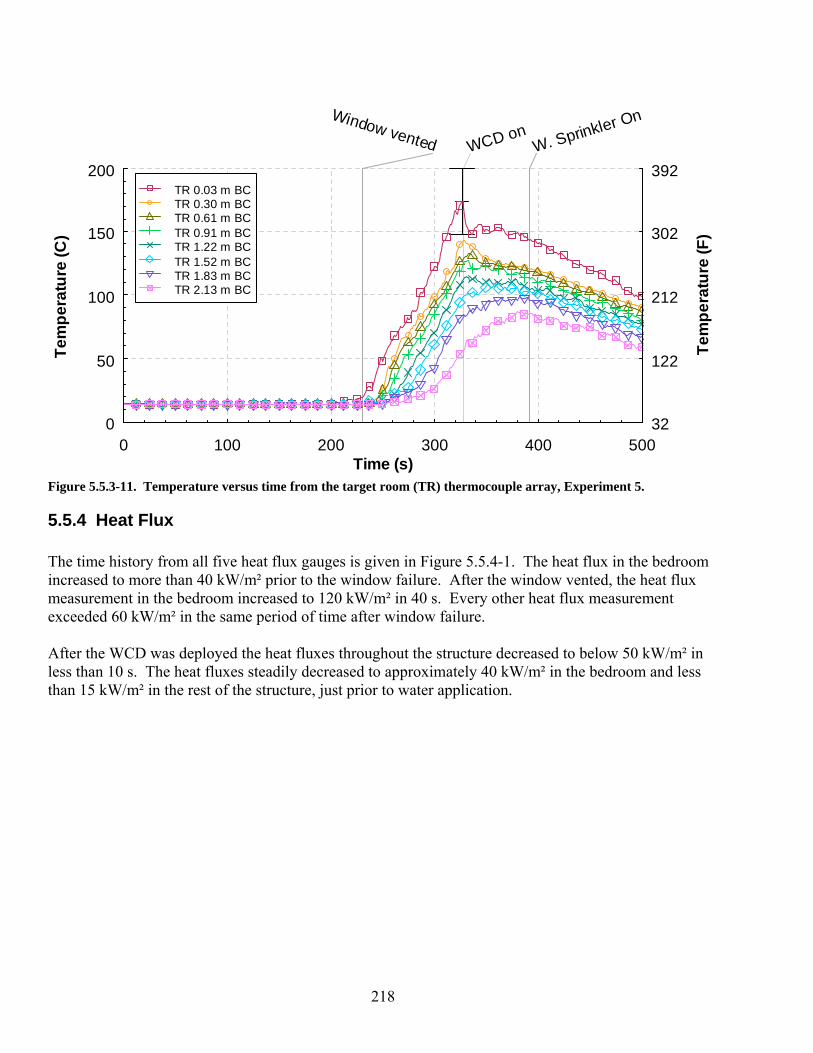
218
Time (s)
Tem
pera
ture
(C)
Window vented WCD onW. Sprinkler On
0 100 200 300 400 5000
50
100
150
200
32
122
212
302
392
Tem
pera
ture
(F)
TR 0.03 m BC TR 0.30 m BC TR 0.61 m BC TR 0.91 m BC TR 1.22 m BC TR 1.52 m BC TR 1.83 m BC TR 2.13 m BC
Figure 5.5.3-11. Temperature versus time from the target room (TR) thermocouple array, Experiment 5.
5.5.4 Heat Flux The time history from all five heat flux gauges is given in Figure 5.5.4-1. The heat flux in the bedroom increased to more than 40 kW/m² prior to the window failure. After the window vented, the heat flux measurement in the bedroom increased to 120 kW/m² in 40 s. Every other heat flux measurement exceeded 60 kW/m² in the same period of time after window failure. After the WCD was deployed the heat fluxes throughout the structure decreased to below 50 kW/m² in less than 10 s. The heat fluxes steadily decreased to approximately 40 kW/m² in the bedroom and less than 15 kW/m² in the rest of the structure, just prior to water application.

219
Time (s)
Hea
t Flu
x (k
W/m
²)Window vented WCD on
W. Sprinkler On
0 100 200 300 400 5000
30
60
90
120
150 BR HF LR HF CC HF CS HF CN HF
Figure 5.5.4-1. Heat flux versus time at five locations, Experiment 5.
5.5.5 Pressure Figure 5.5.5-1 shows the pressures at the 5 measurement locations. There was little pressure change in the structure prior to window failure. After window failure the pressures in the structure increased and became fairly steady. The closer to the source of the simulated wind the higher the pressure was. The bedroom pressure increased to an average of 55 Pa, the hallway and living room pressure increased to approximately 35 Pa, the dead end side of the corridor increased to approximately 20 Pa and the vent side of the corridor increased to 10 Pa. After the WCD was deployed all of the pressures in the structure transitioned to negative. As the pressure stabilized, the pressure in the bedroom decreased to approximately -25 Pa and the pressures decreased to -30 Pa at the vent end of the corridor. While all of the pressures were negative, the gases were still able to flow from a higher pressure (bedroom) to a lower pressure (corridor vent). The magnitude of the negative pressure was created by the flow of hot gases out of the structure and the lack of available make-up air, creating a partial vacuum. The application of water had little to no impact on the pressures, but as the structure cooled the pressures slowly increased.

220
Time (s)
Pres
sure
(Pa)
Window vented WCD onW. Sprinkler On
0 100 200 300 400 500-60
-30
0
30
60
90
BR DP Hall DP LR DP CSW DP CNW DP
Figure 5.5.5-1. Pressure versus time at five locations, Experiment 5.
5.5.6 Velocities Figure 5.5.6-1 provides the velocity measurements from the bi-directional probes that are located outside of the window. The positive velocities were flowing into the window. There was a fluctuation of velocities at the window as the hot gases were trying to exit the window opening while the simulated wind was forcing the gases back into the window. The average velocities shown in the graph indicate that the flow was mainly into the window at the middle and bottom probes and out of the window at the top probe once the room transitioned to flashover. Velocities ranged from 6 m/s (13.4 mph) into the window to 6 m/s (13.4 mph) out of the window. After the WCD was deployed the reading are not reliable as the WCD was pushed up against all of the probes. Figure 5.5.6-2 shows the velocities at the hall array position. On this graph, the positive direction is from west to east. The probe located 0.3 m (1 ft) below the ceiling captures the velocity of the ceiling jet as it moved down the hall away from the bedroom and peaked at approximately 3.0 m/s (6.7 mph) prior to window failure. After window failure the velocity increases to above 5 m/s (11.2 mph) at the top probe and 7 m/s to 10 m/s at the middle and bottom measurement locations. The top probe read lower because of the impact of the size of the doorway. The lintel, which extended 0.4 m (1.3 ft) below the ceiling, slowed the flow or caused turbulence which slowed the flow. Figure 5.5.6-3 displays the velocities from the south corridor position. The positive direction is from north to south. This was the dead end side of the corridor so there was no steady flow through this area. There was a lot of recirculation and changes in the magnitude of the velocity. Flows ranged from -1 m/s to 2 m/s while the wind was flowing through the structure. With the WCD in place the flow became steady between 0 m/s at the bottom probe and 2 m/s at the top probe, toward the vent.

221
The velocities from the north corridor position are shown in Figure 5.5.6-4. The positive flow direction for this location is from south to north. Prior to window failure, the ceiling jet/hot gas layer velocities reached a peak of approximately 0.6 m/s (1.4 mph) at 0.3 m (1 ft) below the ceiling. After the window vented the velocities increased to a peak of approximately 7 m/s (15.7 mph) and a range of 3.5 m/s to 7.5 m/s. The velocities decreased to a range of 1 m/s to 2 m/s after WCD deployment and nozzle activation. The measurements from the bi-directional probes installed in the exhaust vent, 2.44 m (8.0 ft) above the ceiling are given in Figure 5.5.6-5. The flow direction up and out of the structure is positive in the figure. Prior to the window being vented the peak flow velocity is less than 2 m/s (4.5 mph). After the window was vented, the velocities at all three probes were similar and flowing out of the structure at a speed of approximately 7 m/s (15.7) to 9 m/s (20.1 mph). After WCD deployment, the velocities decreased to 1 m/s to 3 m/s but were still unidirectional out of the structure. The activation of the low flow nozzle had little impact on the vent flow velocity.
Time (s)
Velo
city
(m/s
)
Window vented WCD onW. Sprinkler On
0 100 200 300 400 500-9
-6
-3
0
3
6
9
-20
-13
-7
0
7
13
20
Velo
city
(mph
)
BRW BP Top BRW BP Mid BRW BP Bot
Figure 5.5.6-1. Velocity versus time from the bedroom window (BRW) bi-directional probe array, Experiment 5.

222
Time (s)
Velo
city
(m/s
)
Window vented WCD onW. Sprinkler On
0 100 200 300 400 500-3
0
3
6
9
12
-7
0
7
13
20
27
Velo
city
(mph
)
Hall BP 0.30 m BC Hall BP 1.22 m BC Hall BP 2.13 m BC
Figure 5.5.6-2. Velocity versus time from the hall bi-directional probe array, Experiment 5.
Time (s)
Velo
city
(m/s
)
Window vented WCD onW. Sprinkler On
0 100 200 300 400 500-1
0
1
2
3
-2
0
2
4
7
Velo
city
(mph
)
CS BP 0.30 m BC CS BP 1.22 m BC CS BP 2.13 m BC
Figure 5.5.6-3. Velocity versus time from the corridor south (CS) bi-directional probe array, Experiment 5.

223
Time (s)
Velo
city
(m/s
)Window vented WCD on
W. Sprinkler On
0 100 200 300 400 500-2
0
2
4
6
8
10
-4
0
4
9
13
18
22
Velo
city
(mph
)
CN BP 0.30 m BC CN BP 1.22 m BC CN BP 2.13 m BC
Figure 5.5.6-4. Velocity versus time from the corridor north (CN) bi-directional probe array, Experiment 5.
Time (s)
Velo
city
(m/s
)
Window vented WCD onW. Sprinkler On
0 100 200 300 400 500-2
0
2
4
6
8
10
-4
0
4
9
13
18
22
Velo
city
(mph
)
V West BP V Cen BP V East BP
Figure 5.5.6-5. Velocity versus time from the ceiling vent (V) bi-directional probe array, Experiment 5.

224
5.5.7 Gas Concentrations Figure 5.5.7-1 shows the gas concentration measurements made in the lower level of the bedroom. The upper gas sampling probe for the bedroom did not function correctly and was not included. The gas concentrations in the lower portion of the bedroom began to change at approximately 190 s, as the hot gas layer developed and extended down 1.83 m (6.0 ft) from the ceiling to interact with the sampling probe. Just prior to window failure the oxygen concentration decreased to 10 % and the CO2 concentration increased to 10 %. After the window vented at 230 s, the fresh air came in through the window and mixed with the lower portion of the hot gas layer, which temporarily increased the oxygen and decreased the carbon dioxide and carbon monoxide for about 30 s. After this mixing, the oxygen quickly dropped to below 3 %, the CO2 increased to 14 % and the CO increased to 6 %. After the WCD was deployed the oxygen decreased from 3 % to 1 %. Similar trends took place in the CO2 and CO readings as they both increased approximately 3 %. Figure 5.5.7-2 and Figure 5.5.7-3 provide the measurements from the upper and lower gas sampling probes, respectively, in the living room. The magnitudes and trends of the living room gas concentrations are very similar to those of the bedroom. One main difference is a smaller impact when air was introduced by the failing of the window. Much of the oxygen entering the window was consumed by the fire in the bedroom and it did not make it to the living room. The oxygen concentration in the living room at the top and bottom probed dropped to 1 % before deploying the WCD. The CO2 reached as high as 19 % and the CO readings peaked at 4 % prior to WCD deployment and 7 % afterwards. Figure 5.5.7-3 also includes the total hydrocarbon readings from the upper gas sampling probe in the living room. The total hydrocarbon readings begin to increase at about the same time as the CO readings but continue to increase to a peak of 13 % with the WCD in place and the oxygen concentration at a minimum. The concentration decreases after the activation of the low flow nozzle.

225
Time (s)
Gas
Con
cent
ratio
n (%
Vol
ume)
Window vented WCD onW. Sprinkler On
0 100 200 300 400 5000
5
10
15
20
25
BR Lower O2 BR Lower CO2 BR Lower CO
Figure 5.5.7-1. Oxygen, carbon dioxide, and carbon monoxide percent volume versus time from the lower bedroom
(BR) sampling location, Experiment 5.
Time (s)
Gas
Con
cent
ratio
n (%
Vol
ume)
Window vented WCD onW. Sprinkler On
0 100 200 300 400 5000
5
10
15
20
25
LR Upper O2 LR Upper CO2 LR Upper CO LR Upper THC
Figure 5.5.7-2. Oxygen, carbon dioxide, carbon monoxide, and total hydrocarbon percent volume versus time from
the upper living (LR) room sampling location, Experiment 5.

226
Time (s)
Gas
Con
cent
ratio
n (%
Vol
ume)
Window vented WCD onW. Sprinkler On
0 100 200 300 400 5000
5
10
15
20
25
LR Lower O2 LR Lower CO2 LR Lower CO
Figure 5.5.7-3. Oxygen, carbon dioxide, and carbon monoxide percent volume versus time from the lower living room
(LR) sampling location, Experiment 5.
5.6 External Water Application (indirect attack) WDF 6 (fog) The sixth experiment in the series was conducted to examine the impact of wind on the structure fire and quantify the impact of externally applied water sprays. After the window vented and the fire was observed to be fully developed, the window sprinkler, flowing 1.9 L/s (30 gpm), was activated, followed by the addition of a fog spray on the fire environment in the structure. The fog spray originated from an adjustable fog nozzle at the narrow setting (approximately 30º), flowing approximately 5.0 L/s (80 gpm). Initially the fog spray was discharged parallel to the west wall of the structure in front of the window opening. The spray was stopped and the nozzle, with the same settings, was repositioned to discharge directly into the window opening, such that the spray pattern nearly filled the window opening. The experimental preparations were made as described in Section 4. The fan speed used in this experiment was 1500 RPM, which provided a 3.0 m/s to 4.0 m/s (7 mph to 9 mph) wind speed at the window opening. A trash container fuel package was ignited remotely with and electric match to start the experiment at Time = 0 s. A time line of the experiment is presented in Table 5.6-1. The results for the experiment are presented in the following sections: observations, heat release rate, temperature, heat flux, pressure, velocity, and gas concentrations. An uncertainty range marker is included in each graph. Table 5.6-1. Experiment 6 Timeline Time (s) Event
0 Ignition 60 Visible smoke layer
165 Window vented 168 Hot gas flow to floor in corridor IR

227
171 Window cleared 267 Window sprinkler on 293 Stream across window 330 Hose off 347 Stream Into window 395 Fan off 403 Begin suppression 427 Fire out 432 Sprinkler off 457 Fan on 537 Test complete
5.6.1 Observations The observations are presented as a series of images captured from eight camera locations, six were video cameras and two were thermal imaging cameras. The camera positions are shown in Figure 4.1.3-1. Figure 5.6.1-1 through Figure 5.6.1-15, present sets of eight images one from each camera position, at a given time, from the time of ignition to 420 s after ignition. Each image view is labeled. The first four views at the top of each figure show the west wall and window of the structure and then follow a path through the interior of the structure with a view of the bed room, the living room and a view (looking west) through the open door to the corridor. The second set of four views, at the bottom of each figure, provides a video view of the north east portion of the corridor and a view of the inside of the target room door. The thermal imaging cameras provide a view of the east corridor, looking north, and a view of the inside of the target room. Figure 5.6.1-1 shows the conditions at the time of ignition. At this point, the six video views are clear and unobstructed. However, the thermal images provide limited thermal contrast, because the surfaces in the view were at nearly equal temperature. The images in Figure 5.6.1-2 were captured 60 s after ignition. The fire from the trash container began to spread to the bed. Light colored smoke was produced and a thin smoke layer had developed across the ceiling of the bedroom. There was no smoke or change in thermal condition, in the living room, target room or corridor at this time. The images in Figure 5.6.1-3 were recorded at 120 s after ignition. The fire had spread to the area between the bed and the upholstered chair with a flame height of approximately 1.2 m (4.0 ft) above the floor. The smoke layer was approximately 1.2 m (4.0 ft) thick throughout the bedroom. Smoke was beginning to spread through the hallway and into the living room. Small amounts of smoke and heat had reached the corridor at 120 s. The target room appeared clear of smoke. The window vented due to the heat transferred from flame impingement at 165 s after ignition. Figure 5.6.1-4 shows the images recorded at 174 s after ignition, just after the window opening had been completely cleared. The flames can be seen flowing out of the window and across the end of the bed. The living room, doorway and corridor views have been obscured. The thermal image from the corridor

228
shows that heat has filled the living room doorway from top to bottom and that the flow had extended across the corridor and impinged on the east wall. A thin layer of smoke has flowed into the target room. The thermal image from the target room shows the heat flowing in around the upper perimeter of the door. Figure 5.6.1-5 shows the conditions at 180 s after ignition. Flames are seen filing the bedroom and moving across the floor level. The camera views in the living room, hallway and corridor are still obscured by smoke. Conditions in the image from the corridor IR camera and the target room views have not changed much since the previous figure. Figure 5.6.1-6 was captured at 192 s after ignition. Flames were pulsing out of the top of the window opening. Flames can be seen in the bedroom at the floor level, coming through the hallway and into the living room. Flames are also shown extending out through the doorway into the corridor. The metal door to the target room had flames coming from the top right corner and from under the door. The smoke layer in the target room had increased in thickness. The thermal image from the target room exhibits heat moving into the target room from the entire perimeter of the steel door. Figure 5.6.1-7 shows the conditions at 240 s after ignition. Flames were pulsing out of the window opening. Smoke was obscuring the views in the bedroom, living room and corridor. The amount of heat entering the hallway has caused the image from the corridor IR camera to deteriorate substantially. The visual image in the target room showed flames continuing to burn under the door. The visibility at the lower layer in the target room remained good. The images in Figure 5.6.1-8 were recorded at 265 s after ignition, a few second before the window sprinkler was activated. Flames appeared to fill the entire bedroom. The views from the inside the bedroom, living room, and corridor were completely obscured by smoke. The thermal view of the corridor continued to show large quantities of heat but the ability to view any of the structure was lost. The target room video view continued to show flames around the bottom of the target room door. The thermal view shows the outlines of the metal door detail, as the door had increased in temperature. At 287 s after ignition, the images in Figure 5.6.1-9 were recorded. The window sprinkler had been activated for 20 s. Flames stilled pulsed from the window opening. The flames near the window appeared to be partially blocked by soot. The interior video views were still obscured, only a glow was visible in the bedroom view. The thermal view of the corridor was obscured due to high thermal conditions. Conditions in the target room had decayed as the hot gas layer dropped within 0.30 m (1.0 ft) of the floor. Flames were still visible under the door to the hallway. In the thermal image of the target room door, the door had become whiter in color, indicating that had become hotter. Figure 5.6.1-10 shows the conditions at 300 s after ignition, or approximately 8 s after the water fog was started across the window opening. The interior video views were still obscured by smoke. The thermal image from the corridor was still saturated due to high heat conditions. In the target room, the smoke layer was near the floor, flames were no longer visible coming under the door. The door continued to heat up, as shown in the target room thermal view. Figure 5.6.1-11 shows the conditions at 330 s after ignition, just as the fog water was shut off. The window sprinkler was still activated. The area in the center of the window opening was free from fire.

229
All of the interior video views were still obscured by soot. The corridor thermal image shows more contrast indicating that the thermal conditions in that location had cooled. The target room thermal image shows that the door remained hot. The images in Figure 5.6.1-12 were recorded at 345 s after ignition, just prior to the activation of the fog stream into the window opening. The volume of flame visible through the window opening had decreased. All of the interior video views were obscured by smoke. The thermal images showed cooler conditions in the corridor and a hotter target room door when compared with the previous figure. Figure 5.6.1-13 shows the conditions 13 s after the fog spray directly into the window was started. The images seem similar to the images in Figure 5.6.1-12. The images in Figure 5.6.1-14 were recorded after 50 s of direct, fog stream application. The flames in the bedroom had decreased. The interior video views were still obscured. The corridor thermal view shows continued cooling. The black area on the east wall across from the door is indicative of the wall cooling due to the water. Portions of the target room door appear to have been impacted by the water in the areas that appear dark. The post-test images are shown in Figure 5.6.1-15. The fire in the bedroom had been suppressed. The conditions in the corridor continued to cool. All other views had not changed. Post test inspection indicated that the protective covers for the interior video cameras were coated with soot.

230
Figure 5.6.1-1. Experiment 6, ignition.

231
Figure 5.6.1-2. Experiment 6, 60 s after ignition.

232
Figure 5.6.1-3. Experiment 6, 120 s after ignition.

233
Figure 5.6.1-4. Experiment 6, window fully vented, 174 s after ignition.

234
Figure 5.6.1-5. Experiment 6, 180 s after ignition.

235
Figure 5.6.1-6. Experiment 6, corridor flames, 192 s after ignition.

236
Figure 5.6.1-7. Experiment 6, 240 s after ignition.

237
Figure 5.6.1-8. Experiment 6, 265 s after ignition.

238
Figure 5.6.1-9. Experiment 6, 287 s after ignition, 20 s after window sprinkler activation.

239
Figure 5.6.1-10. Experiment 6, 300 s after ignition.

240
Figure 5.6.1-11. Experiment 6, fog stream across window off, 330 s after ignition.

241
Figure 5.6.1-12. Experiment 6, direct fog stream on, 345 s after ignition.

242
Figure 5.6.1-13. Experiment 6, 360 s after ignition.

243
Figure 5.6.1-14. Experiment 6, 400 s after ignition.

244
Figure 5.6.1-15. Experiment 6, 420 s after ignition.

245
5.6.2 Heat Release Rate Figure 5.6.2-1 shows the heat release rate time history for Experiment 6. The increase in measured heat release rate is delayed because for the first 160 s after ignition because no heat or combustion products generated by the fire flowed out of the structure. After the window failed, at 165 s after ignition, the increase in heat release rate was clear. The heat release rate reached a peak of approximately 17 MW, 45 s after window failure, followed by a quick drop to 8 MW and return to 15 MW over the next 30 s. The window sprinkler was activated at 267 s and hose was sprayed across the window at 293 s which caused the heat release rate to drop to just above 10 MW. At 347 s, the hose stream was shut off, repositioned in front of the window and reactivated. This action actually increased the heat release rate to a peak of approximately 16 MW for about 30 s but ultimately caused a drastic heat release rate reduction. At 395 s, the fan was shut off and manual suppression ended the test shortly thereafter.
Time (s)
Hea
t Rel
ease
Rat
e (M
W)
Window vented
W.Sprinkler on
Stream Across W
.Hose off
Stream Into W
. Fan
off
Begin
Sup
pres
sion
Fire
out
Sprin
kler o
ffFa
n on
0 100 200 300 400 5000
5
10
15
20
Figure 5.6.2-1. Heat release rate versus time, Experiment 6.
5.6.3 Temperatures Figure 5.6.3-1 through Figure 5.6.3-11 provides the temperature measurements from the thermocouple arrays shown in Figure 4.1.3-1. The figures are given in order from the western most measurement point, the bed room window opening, and moving through the structure toward the east; bedroom, hall,

246
living room, corridor, south and southwest portions of the corridor (closed end) and then to the north section of the corridor and ending with the exhaust vent. The last temperature graph has temperatures associated with the target room. The three thermocouples located in the window opening, shown in Figure 5.6.3-1, provide insight into the ventilation conditions at the window. After window failure at 165 s temperatures fluctuate as the flames are pulsing out of the window and wind is blowing into the window. The highest temperatures are located in the top of the window opening. Activation of the window sprinkler at 267 s as well as use of the fog hose stream across and into the window reduced the temperatures at the window from a peak of 550 ºC (1022 ºF) to less than 50 ºC (122 ºF) in the span of 100 s. The measurements from the thermocouple array located in the center of the bedroom are given in Figure 5.6.3-2. Prior to the window failure, the temperatures in the bedroom increased from ambient conditions to a peak of approximately 650 ºC (1202 ºF) near the ceiling. At the same time, the temperatures, 2.13 m (7.00 ft) below the ceiling, were almost 50 ºC (122 ºF). Flashover conditions were reached, based on temperatures from ceiling to floor being in excess of 900 ºC (1652 ºF), at approximately 200 s after ignition and 40 s after window failure. Activation of the window sprinkler at 267 s reduced all temperatures in the room and use of the fog stream across the window further decreased all levels to less than 300 ºC (572 ºF). As the hose stream was shut off, repositioned in directly into the window and turned back on again, the temperatures in the room stratified and the upper half of the room began to increase. Temperatures near the ceiling topped 600 ºC (1112 ºF) while the floor remained at ambient conditions. The data from the hall thermocouple array is presented in Figure 5.6.3-3. The temperatures slowly increased and stratified as the fire in the bedroom developed. The ceiling temperature in the hallway reached approximately 350 ºC (662 ºF), while the temperature 2.13 m (7.00 ft) below the ceiling was still ambient just prior to window failure. 30 s after window failure the temperatures peaked to 950 ºC (1742 ºF) at the ceiling, but then decreased for 50 s. At 250 s, all temperatures returned to the peak level until the window sprinkler was activated. The window sprinkler, combined with the fog stream across the window cut all temperatures down to 50 ºC (122 ºF). When the hose stream was redirected into the window, temperatures restratified and began to increase up to 300 ºC (572 ºF) in the upper layers of the hallway. The data from the living room corner thermocouple array is shown in Figure 5.6.3-4. 20 s after window failure, the temperatures from floor to ceiling were in excess of 600 ºC (1112 ºF). No significant change in temperature conditions were noted with the use of the window sprinkler or the fog stream across the window. When the hose stream was directed into the window, temperatures in the hallway increased to just below 800 ºC (1472 ºF) for 20 s but then fell below 400 ºC (752 ºF) prior to the end of the test. The temperatures from the center of the living room are shown in Figure 5.6.3-5 for the time history of the experiment. Again, there was a dramatic temperature increase seconds after the window failure. As the hot gases were forced through the living room the temperatures elevated from 300 ºC (572 ºF) at the ceiling and ambient at the floor to 800 ºC (1472 ºF) from floor to ceiling. Temperatures decreased for the next 50 s but then began to increase even with the window sprinkler activation. The use of the fog stream across the window at 293 s, however, caused temperatures to drop to 550 ºC (1022 ºF) and stabilize for a short time period. When the stream was redirected into the window, temperatures began

247
to increase once again for approximately 20 s but then declined significantly to levels below 300 ºC (572 ºF). Temperature conditions in the corridor are given in Figure 5.6.3-6 through Figure 5.6.3-9. Temperature records for the center and north corridor regions were similar in nature but were slightly different in scale. The center and north regions peaked at 800 ºC (1472 ºF) 30 s after window failure then reduced in temperature 600 ºC (1112 ºF) . Window sprinkler activation and the fog stream application across the window steadily increased temperatures up until the fog stream was redirected into the window but the center region topped out at 800 ºC (1472 ºF) while the north region hit 950 ºC (1742 ºF). Fog stream application into the window significantly decreased temperatures in both regions throughout the remainder of the test. The south and southwest regions of the corridor both rapidly increased in temperature 30 s after window failure with the south reaching 600 and southwest reaching 350 at the ceiling. Both regions were more stratified in nature and declined slightly or remained relatively constant until the fog stream was directed into the window. The window sprinkler and fog application across the window did not have a significant effect on temperature differences. Directing the fog stream into the window increased both the south and southwest corridor regions for approximately 10 s before all temperatures declined to the end of the test. The temperatures at the exhaust vent are given in Figure 5.5.3-10. These thermocouples were at the same elevation located 2.44 m (8 ft) above the ceiling of the corridor. The three thermocouples were spaced 0.51 m (1.67 ft) apart along the east-west centerline of the vent. These temperatures increased from less than 100 ºC (212 ºF) to greater than 600 ºC (1112 ºF) in about 30 s following window failure. Temperatures increased with the use of the window sprinkler and fog stream application both across and into the window to a peak of 1000 ºC (1832 ºF). 10 s prior to shutting the fan off, temperatures drastically reduced for the rest of the test period. The final temperature graph displays the temperature time history for the target room (Figure 5.5.3-11). All of the temperatures remained near ambient until the window failed. After window failure, temperatures stratified and continually increased until the hose stream was applied across the window. The temperatures leveled off at this point, with ceiling and floor temperatures measuring 140 ºC (284 ºF) and 80 ºC (176 ºF) respectively, but remained stratified until 10 s prior to shutting the fan off. After the fan was shut off, temperatures suddenly collectively to 60 ºC (140 ºF) but then began to increase at a steady state once again.

248
Time (s)
Tem
pera
ture
(C)
Window vented
W.Sprinkler on
Stream Across W
.Hose off
Stream Into W
. Fan
off
Begin
Sup
pres
sion
Fire
out
Sprin
kler o
ffFa
n on
0 100 200 300 400 5000
200
400
600
800
32
392
752
1112
1472
Tem
pera
ture
(F)
BRW TC Top BRW TC Mid BRW TC Bot
Figure 5.6.3-1. Temperature versus time from the bedroom window (BRW) thermocouple array, Experiment 6.

249
Time (s)
Tem
pera
ture
(C)
Window vented
W.Sprinkler on
Stream Across W
.Hose off
Stream Into W
. Fan
off
Begin
Sup
pres
sion
Fire
out
Sprin
kler o
ffFa
n on
0 100 200 300 400 5000
300
600
900
1200
32
572
1112
1652
2192
Tem
pera
ture
(F)
BR 0.03 m BC BR 0.30 m BC BR 0.61 m BC BR 0.91 m BC BR 1.22 m BC BR 1.52 m BC BR 1.83 m BC BR 2.13 m BC
Figure 5.6.3-2. Temperature versus time from the bedroom (BR) thermocouple array, Experiment 6.

250
Time (s)
Tem
pera
ture
(C)
Window vented
W.Sprinkler on
Stream Across W
.Hose off
Stream Into W
. Fan
off
Begin
Sup
pres
sion
Fire
out
Sprin
kler o
ffFa
n on
0 100 200 300 400 5000
300
600
900
1200
1500
32
572
1112
1652
2192
2732
Tem
pera
ture
(F)
Hall 0.03 m BC Hall 0.30 m BC Hall 0.61 m BC Hall 0.91 m BC Hall 1.22 m BC Hall 1.52 m BC Hall 1.83 m BC Hall 2.13 m BC
Figure 5.6.3-3. Temperature versus time from the hall thermocouple array, Experiment 6.

251
Time (s)
Tem
pera
ture
(C)
Window vented
W.Sprinkler on
Stream Across W
.Hose off
Stream Into W
. Fan
off
Begin
Sup
pres
sion
Fire
out
Sprin
kler o
ffFa
n on
0 100 200 300 400 5000
200
400
600
800
1000
32
392
752
1112
1472
1832
Tem
pera
ture
(F)
LRC 0.03 m BC LRC 0.30 m BC LRC 0.61 m BC LRC 0.91 m BC LRC 1.22 m BC LRC 1.52 m BC LRC 1.83 m BC LRC 2.13 m BC
Figure 5.6.3-4. Temperature versus time from the living room corner (LRC) thermocouple array, Experiment 6.

252
Time (s)
Tem
pera
ture
(C)
Window vented
W.Sprinkler on
Stream Across W
.Hose off
Stream Into W
. Fan
off
Begin
Sup
pres
sion
Fire
out
Sprin
kler o
ffFa
n on
0 100 200 300 400 5000
300
600
900
1200
32
572
1112
1652
2192
Tem
pera
ture
(F)
LR 0.03 m BC LR 0.30 m BC LR 0.61 m BC LR 0.91 m BC LR 1.22 m BC LR 1.52 m BC LR 1.83 m BC LR 2.13 m BC
Figure 5.6.3-5. Temperature versus time from the living room (LR) thermocouple array, Experiment 6.

253
Time (s)
Tem
pera
ture
(C)
Window vented
W.Sprinkler on
Stream Across W
.Hose off
Stream Into W
. Fan
off
Begin
Sup
pres
sion
Fire
out
Sprin
kler o
ffFa
n on
0 100 200 300 400 5000
200
400
600
800
1000
32
392
752
1112
1472
1832
Tem
pera
ture
(F)
CC 0.03m BC CC 0.30 m BC CC 0.61 m BC CC 0.91 m BC CC 1.22 m BC CC 1.52 m BC CC 1.83 m BC CC 2.13 m BC
Figure 5.6.3-6. Temperature versus time from the corridor center (CC) thermocouple array, Experiment 6.

254
Time (s)
Tem
pera
ture
(C)
Window vented
W.Sprinkler on
Stream Across W
.Hose off
Stream Into W
. Fan
off
Begin
Sup
pres
sion
Fire
out
Sprin
kler o
ffFa
n on
0 100 200 300 400 5000
200
400
600
800
1000
32
392
752
1112
1472
1832
Tem
pera
ture
(F)
CS 0.03 m BC CS 0.30 m BC CS 0.61 m BC CS 0.91 m BC CS 1.22 m BC CS 1.52 m BC CS 1.83 m BC CS 2.13 m BC
Figure 5.6.3-7. Temperature versus time from the corridor south (CS) thermocouple array, Experiment 6.

255
Time (s)
Tem
pera
ture
(C)
Window vented
W.Sprinkler on
Stream Across W
.Hose off
Stream Into W
. Fan
off
Begin
Sup
pres
sion
Fire
out
Sprin
kler o
ffFa
n on
0 100 200 300 400 5000
100
200
300
400
500
32
212
392
572
752
932
Tem
pera
ture
(F)
CSW 0.03 m BC CSW 0.30 m BC CSW 0.61 m BC CSW 0.91 m BC CSW 1.22 m BC CSW 1.52 m BC CSW 1.83 m BC CSW 2.13 m BC
Figure 5.6.3-8. Temperature versus time from the corridor southwest (CSW) thermocouple array, Experiment 6.

256
Time (s)
Tem
pera
ture
(C)
Window vented
W.Sprinkler on
Stream Across W
.Hose off
Stream Into W
. Fan
off
Begin
Sup
pres
sion
Fire
out
Sprin
kler o
ffFa
n on
0 100 200 300 400 5000
300
600
900
1200
32
572
1112
1652
2192
Tem
pera
ture
(F)
CN 0.03 m BC CN 0.30 m BC CN 0.61 m BC CN 0.91 m BC CN 1.22 m BC CN 1.52 m BC CN 1.83 m BC CN 2.13 m BC
Figure 5.6.3-9. Temperature versus time from the corridor north (CN) thermocouple array, Experiment 6.

257
Time (s)
Tem
pera
ture
(C)
Window vented
W.Sprinkler on
Stream Across W
.Hose off
Stream Into W
. Fan
off
Begin
Sup
pres
sion
Fire
out
Sprin
kler o
ffFa
n on
0 100 200 300 400 5000
300
600
900
1200
32
572
1112
1652
2192
Tem
pera
ture
(F)
Vent West TC Vent Center TC Vent East TC
Figure 5.6.3-10. Temperature versus time from the ceiling vent thermocouple array, Experiment 6.

258
Time (s)
Tem
pera
ture
(C)
Window vented
W.Sprinkler on
Stream Across W
.Hose off
Stream Into W
. Fan
off
Begin
Sup
pres
sion
Fire
out
Sprin
kler o
ffFa
n on
0 100 200 300 400 5000
100
200
300
32
212
392
572
Tem
pera
ture
(F)
TR 0.03 m BC TR 0.30 m BC TR 0.61 m BC TR 0.91 m BC TR 1.22 m BC TR 1.52 m BC TR 1.83 m BC TR 2.13 m BC
Figure 5.6.3-11. Temperature versus time from the target room (TR) thermocouple array, Experiment 6.
5.6.4 Heat Flux The time history from all five heat flux gauges is given in Figure 5.6.4-1. The heat flux in the bedroom increased to 20 kW/m² prior to the window failure. After the window vented, the heat flux measurement in the bedroom increased to just less than 200 kW/m² in 90 s but dropped very quickly once the sprinkler activated. The bedroom heat flux continued down to near ambient for the remainder of the test. All other heat flux measurements also had a quick increase during the first 60 s of the test but reduced in value shortly after. The window sprinkler activation and associated hose stream applications increased the heat flux measurements but were sporadic in nature.

259
Time (s)
Hea
t Flu
x (k
W/m
²)
Window vented
W.Sprinkler on
Stream Across W
.Hose off
Stream Into W
. Fan
off
Begin
Sup
pres
sion
Fire
out
Sprin
kler o
ffFa
n on
0 100 200 300 400 5000
50
100
150
200
250 BR HF LR HF CC HF CS HF CN HF
Figure 5.6.4-1. Heat flux versus time at five locations, Experiment 6.
5.6.5 Pressure Figure 5.6.5-1 shows the pressures at the 5 measurement locations. There was little pressure change in the structure up to just prior to window failure. After window failure, the pressures in the structure increased at first, then declined but increased again over the span of 100 s. The closer to the source of the simulated wind the higher the pressure was. Pressures in the northwest and southwest corridors changed directions several times indicating a circulating air flow. The window sprinkler and fog stream across the window reduced all pressure values significantly but redirecting the stream into the window greatly increased the values once again. The bedroom, hallway and living room all peaked at 60 Pa while the southwest and northwest corridors hit 45 Pa and 30 Pa respectively. All pressures were reduced to 0 Pa once the fan was shut off.

260
Time (s)
Pres
sure
(Pa)
Window vented
W.Sprinkler on
Stream Across W
.Hose off
Stream Into W
. Fan
off
Begin
Sup
pres
sion
Fire
out
Sprin
kler o
ffFa
n on
0 100 200 300 400 500-20
0
20
40
60
80 BR DP Hall DP LR DP CSW DP CNW DP
Figure 5.6.5-1. Pressure versus time at five locations, Experiment 6.
5.6.6 Velocities Figure 5.6.6-1 provides the velocity measurements from the bi-directional probes that are located outside of the window. The positive velocities were flowing into the window. All bedroom window velocities increased to 1 m/s (2.2 mph) after the window failed and remained somewhat constant until the hose stream was directed across the window. Once the hose stream was redirected, the top pressure varied wildly from -18 m/s (40.2 mph) to +12 m/s (26.8 mph), the middle pressure spiked to 16 m/s (35.8 mph) and the bottom pressure jumped to 10 m/s (22.4 mph) but gradually reduced. Figure 5.6.6-2 shows the velocities at the hall array position. On this graph, the positive direction is from west to east. All three probes recorded an increase in pressure just prior to and continued shortly after the window vented for approximately 40 s. The probes located at 1.22 m (4 ft) and 2.13 m (7 ft) each reached 8 m/s (17.9 mph) and remained relatively constant while the probe at 0.3 m (1 ft) reached 4 m/s (8.9 mph) and remained constant as well. When the sprinkler was activated and fog stream applied across the window, all three pressures reduced to 2 m/s (4.5 mph). However, when the hose stream was redirected into the window, the probes at 1.22 m (4 ft) and 2.13 (7 ft) began to oscillate while the probe at 0.3 m (1 ft) reduced to 0 m/s (0 mph). Figure 5.6.6-3 displays the velocities from the south corridor position. The positive direction is from north to south. This was the dead end side of the corridor so there was no steady flow through this area.

261
There was significant recirculation and changes in the magnitude of the velocity. Flows ranged from -0.6 m/s to 2.2 m/s while the wind was flowing through the structure. The velocities from the north corridor position are shown in Figure 5.6.6-4. The positive flow direction for this location is from south to north. Prior to window failure, the ceiling jet/hot gas layer velocities reached a peak of approximately 0.6 m/s (1.4 mph). After the window vented the velocities increased to a peak of approximately 6 m/s (13.4 mph) but then reduced. When the sprinkler was activated and the hose stream applied across the window, the velocities increased to a range of 5.8 m/s (13.0 mph) to 7.8 m/s (17.4 mph). When the hose stream was redirected through the window, the velocities decreased to a range of 2.0 m/s (4.5 mph) to 5.4 m/s (12.1 mph). The measurements from the bi-directional probes installed in the exhaust vent, 2.44 m (8.0 ft) above the ceiling are given in Figure 5.6.6-5. The flow direction up and out of the structure is positive in the figure. Prior to the window being vented the peak flow velocity is less than 2 m/s (4.5 mph). After the window was vented, the velocities at all three probes were similar and flowing out of the structure at a speed of approximately 7 m/s (15.7 mph). Flowing the fog stream through the window increased the pressures to their peak range of 8 m/s (17.9 mph) to 12 m/s (26.8 mph).
Time (s)
Velo
city
(m/s
)
Window vented
W.Sprinkler on
Stream Across W
.Hose off
Stream Into W
. Fan
off
Begin
Sup
pres
sion
Fire
out
Sprin
kler o
ffFa
n on
0 100 200 300 400 500-30
-20
-10
0
10
20
-67
-45
-22
0
22
45
Velo
city
(mph
) BRW BP Top BRW BP Mid BRW BP Bot
Figure 5.6.6-1. Velocity versus time from the bedroom window (BRW) bi-directional probe array, Experiment 6.

262
Time (s)
Velo
city
(m/s
)
Window vented
W.Sprinkler on
Stream Across W
.Hose off
Stream Into W
. Fan
off
Begin
Sup
pres
sion
Fire
out
Sprin
kler o
ffFa
n on
0 100 200 300 400 500-30
-20
-10
0
10
-67
-45
-22
0
22
Velo
city
(mph
)
Hall BP 0.30 m BC Hall BP 1.22 m BC Hall BP 2.13 m BC
Figure 5.6.6-2. Velocity versus time from the hall bi-directional probe array, Experiment 6.

263
Time (s)
Velo
city
(m/s
)
Window vented
W.Sprinkler on
Stream Across W
.Hose off
Stream Into W
. Fan
off
Begin
Sup
pres
sion
Fire
out
Sprin
kler o
ffFa
n on
0 100 200 300 400 500-1
0
1
2
3
-2
0
2
4
7
Velo
city
(mph
)
CS BP 0.30 m BC CS BP 1.22 m BC CS BP 2.13 m BC
Figure 5.6.6-3. Velocity versus time from the corridor south (CS) bi-directional probe array, Experiment 6.

264
Time (s)
Velo
city
(m/s
)
Window vented
W.Sprinkler on
Stream Across W
.Hose off
Stream Into W
. Fan
off
Begin
Sup
pres
sion
Fire
out
Sprin
kler o
ffFa
n on
0 100 200 300 400 500-2
0
2
4
6
8
10
-4
0
4
9
13
18
22
Velo
city
(mph
)
CN BP 0.30 m BC CN BP 1.22 m BC CN BP 2.13 m BC
Figure 5.6.6-4. Velocity versus time from the corridor north (CN) bi-directional probe array, Experiment 6.

265
Time (s)
Velo
city
(m/s
)
Window vented
W.Sprinkler on
Stream Across W
.Hose off
Stream Into W
. Fan
off
Begin
Sup
pres
sion
Fire
out
Sprin
kler o
ffFa
n on
0 100 200 300 400 500-3
0
3
6
9
12
15
-7
0
7
13
20
27
34
Velo
city
(mph
)
V West BP V Cen BP V East BP
Figure 5.6.6-5. Velocity versus time from the ceiling vent (V) bi-directional probe array, Experiment 6.
5.6.7 Gas Concentrations Figure 5.6.7-1 and Figure 5.6.7-2 show the gas concentration measurements made in the upper and lower levels of the bedroom. The gas concentrations in the upper portion of the bedroom began to change at approximately 100 s, as the hot gas layer developed and extended down 1.83 m (6.0 ft) from the ceiling to interact with the sampling probe. Just prior to window failure, the oxygen concentration decreased to 19 % and the CO2 concentration increased to 2 %. After the window vented, the oxygen concentration dropped to near zero and the CO2 concentration jumped to 10 % along with an increase to 5 % in CO concentration. When the sprinkler activated and the hose stream was applied across the window, the CO2 wavered some, but the oxygen concentration increased and the CO concentration decreased. When the hose stream was redirected into the window, oxygen concentration increased to 16 %, CO2 concentration dropped to 3 % and CO concentration fell to near zero once again. The only increase in total hydrocarbon concentration occurred 80 s after the window vented but a decline gradually occurred for the remainder of the test. The gas concentrations in the lower portion of the bedroom began to change at approximately 150 s, as the hot gas layer developed and extended down 1.83 m (6.0 ft) from the ceiling to interact with the sampling probe. Just prior to window failure the oxygen concentration decreased to 9 % and the CO2 concentration increased to 9 %. After the window vented at 165 s, the fresh air came in through the window and mixed with the lower portion of the hot gas layer, which temporarily increased the oxygen

266
and decreased the carbon dioxide and carbon monoxide for about 30 s. After this mixing, the oxygen quickly dropped to below 5 %, the CO2 increased to 12 % and the CO increased to 3 %. Wavering indicated a mixing of the air prior to sprinkler activation. Once the sprinkler activated and the hose stream applications were applied, an increase in oxygen concentration to 19 % and decreases in CO2 and CO concentrations to 1 % and 0 % respectively occurred. Figure 5.6.7-3 and Figure 5.6.7-4 provide the measurements from the upper and lower gas sampling probes, respectively, in the living room. Gas concentrations in the upper portion of the living room began to change at approximately 180 s. After the window vented, the oxygen concentration dropped from 20 % to near 0 % in the span of 100 s and remained there for the duration of the test. After the window vented, the CO2 concentration jumped from 1 % to a peak of 17 % in the span of 100 s. The sprinkler activation did not have an effect but the fog stream across the window at 293 s caused the level to drop to 14 %. Placing the fog stream directly in the window at 347 s caused an increase to 16 % where is then leveled off. The CO and total hydrocarbon concentrations mirrored each other and initially rose to 5 % just prior to the sprinkler application. A small decrease occurred after sprinkler activation, but the fog stream across the window caused both values to increase once again. However, placing the hose stream into the window reduced both values to 3 %. The gas concentrations in the lower portion of the living room began go change just prior to window ventilation. After the window vented, the oxygen concentration fell from 20 % to 1 % in 40 s and remained relatively constant. An increase to 4 % was noticed when the fog stream was placed into the window at 347 s. The CO2 increased from 1 % to 16 % in 40 s but decreased with each successive application of water to 10 %. The CO concentration jumped from near 0 % to 4 % in 40 s but declined to 3 % with the sprinkler activation. The fog stream flowing across the window caused an increase to 6 % but as the stream was repositioned into the window, the concentration fell back to 4 %.

267
Time (s)
Gas
Con
cent
ratio
n (%
Vol
ume)
Window vented
W.Sprinkler on
Stream Across W
.Hose off
Stream Into W
. Fan
off
Begin
Sup
pres
sion
Fire
out
Sprin
kler o
ffFa
n on
0 100 200 300 400 5000
5
10
15
20
25 BR Upper O2 BR Upper CO2 BR Upper CO BR Upper THC
Figure 5.6.7-1. Oxygen, carbon dioxide, carbon monoxide, and total hydrocarbon percent volume versus time from
the upper bedroom (BR) sampling location, Experiment 6.

268
Time (s)
Gas
Con
cent
ratio
n (%
Vol
ume)
Window vented
W.Sprinkler on
Stream Across W
.Hose off
Stream Into W
. Fan
off
Begin
Sup
pres
sion
Fire
out
Sprin
kler o
ffFa
n on
0 100 200 300 400 5000
5
10
15
20
25
BR Lower O2 BR Lower CO2 BR Lower CO
Figure 5.6.7-2. Oxygen, carbon dioxide, and carbon monoxide percent volume versus time from the lower bedroom
(BR) sampling location, Experiment 6.

269
Time (s)
Gas
Con
cent
ratio
n (%
Vol
ume)
Window vented
W.Sprinkler on
Stream Across W
.Hose off
Stream Into W
. Fan
off
Begin
Sup
pres
sion
Fire
out
Sprin
kler o
ffFa
n on
0 100 200 300 400 5000
5
10
15
20
25
LR Upper O2 LR Upper CO2 LR Upper CO LR Upper THC
Figure 5.6.7-3. Oxygen, carbon dioxide, carbon monoxide, and total hydrocarbon percent volume versus time from
the upper living (LR) room sampling location, Experiment 6.

270
Time (s)
Gas
Con
cent
ratio
n (%
Vol
ume)
Window vented
W.Sprinkler on
Stream Across W
.Hose off
Stream Into W
. Fan
off
Begin
Sup
pres
sion
Fire
out
Sprin
kler o
ffFa
n on
0 100 200 300 400 5000
5
10
15
20
25 LR Lower O2 LR Lower CO2 LR Lower CO
Figure 5.6.7-4. Oxygen, carbon dioxide, and carbon monoxide percent volume versus time from the lower living room
(LR) sampling location, Experiment 6.
5.7 External Water Application (indirect attack) WDF 7 (smooth bore) The seventh experiment in the series was conducted to examine the impact of wind on the structure fire, the impact of closing the doorway from the living room to the corridor, and to quantify the impact of a smooth bore water stream into the bedroom. The experimental preparations were made as described in Section 4. The fan speed used in this experiment was 1500 RPM, which provided a 3.0 m/s to 4.0 m/s (7 mph to 9 mph) wind speed at the window opening. A trash container fuel package was ignited remotely with and electric match to start the experiment at Time = 0 s. A time line of the experiment is presented in Table 5.7-1. The results for the experiment are presented in the following sections: observations, heat release rate, temperature, heat flux, pressure, velocity, and gas concentrations. An uncertainty range marker is included in each graph.

271
Table 5.7-1. Experiment 7 Timeline Time (s) Event
0 Ignition 200 Visible smoke layer 297 Window vented partially 310 Window cleared 377 Door open 435 Hose on, at ceiling 505 Sweeping ceiling 538 Hose off 545 Manual suppression 550 Fire knocked down
5.7.1 Observations The observations are presented as a series of images captured from eight camera locations, six were video cameras and two were thermal imaging cameras. The video camera and thermal imaging camera were removed from the target room and placed outside the structure. The video camera shows the “stack”, which is the extension of the vent into the exhaust hood. The thermal imaging camera shows a similar view as the outside video camera. Figure 5.7.1-1 through Figure 5.7.1-13 present sets of eight images, one from each camera position, at a given time, from the time of ignition to 550 s after ignition. Each image view is labeled. Figure 5.7.1-1 shows the conditions at the time of ignition. At this point, the six video views are clear and unobstructed. However, the thermal images provide limited thermal contrast, because the surfaces in the view were at nearly equal temperature. The images in Figure 5.2.1-2 were captured 60 s after ignition. The fire has yet to extend out of the trash container. A smoke layer was beginning to form in the bedroom. There was no smoke or change in thermal condition in the living room or corridor at this time. The images in Figure 5.2.1-3 were recorded at 120 s after ignition. The fire extended out of the trashcan and extended to the bed and the chair. The smoke layer was still forming in the bedroom. Smoke and heat had just started to flow into the living room. The outside thermal imaging view shows the fire visible through the glass window. The images in Figure 5.7.1-4 were recorded at 180 s after ignition. The fire had spread to the area between the bed and the upholstered chair with a flame height of approximately 0.9 m (3 ft) above the floor. The smoke layer was approximately 0.9 m (3 ft) thick throughout the bedroom. Smoke was beginning to spread through the hallway and into the living room. No smoke and heat had made it into the corridor because the door to the corridor was closed. Figure 5.7.1-5 shows the images recorded 60 s later at 240 s after ignition. The window was still fully intact. The flames were spreading across the side of the bed and onto the back of the chair. The smoke layer was lowering and darkening in the bedroom. A smoke layer was also developed in the living

272
room. A slight haze of smoke was visible in the corridor and the thermal imaging view in the corridor shows some heat leaking around the metal door. No smoke was evident coming from the stack. Figure 5.7.1-6 shows the images at 300 s after ignition. The smoke layer descended to the floor in most of the structure. The corner of the window had cracked and fell out. There was an increase in the amount of heat entering the corridor through cracks around the door and the visibility in the corridor was diminishing. Light smoke was visible from the stack. The images in Figure 5.7.1-7 were recorded 312 s after ignition. The window opening had just been manually cleared. The flames could be seen flowing out of the window opening against the wind. Soot obscured the video views in the bedroom, living room and both of the cameras in the corridor. The image from the corridor IR camera shows hot gases being forced around the door at a higher velocity. Increased smoke was coming from the stack and filling the exhaust hood. Figure 5.7.1-8 shows the conditions at 360 s after ignition. Flames are still flowing out of the top of the window opening. There was very little visibility in the rest of the structure. The door to the corridor was still closed so the heat was being forced around the door and through the hole for the door knob. The stack was being obstructed by smoke as well. The images in Figure 5.7.1-9 were recorded at 420 s after ignition, 43 s after the door to the corridor was opened remotely. The bedroom was completely full of flames and flames were coming out of the window against the simulated wind. All of the internal video camera views were obscured by smoke. The corridor thermal imaging camera was completely saturated with hot gas flow and there is no usable image. At 435 s after ignition, the hose stream was directed at the ceiling of the bedroom as shown in the outside view of Figure 5.7.1-10. The interior video views were still obscured by soot. The heat coming out of the bedroom window was diminished and the stack was still not visible. Figure 5.7.1-11 shows the conditions at 480 s after ignition, or approximately 45 s since activation of the hose stream. The interior video views were still obscured by soot, but the bedroom view was returning to show flames. The thermal image from the corridor was still saturated with heat but started to improve in clarity. The outside thermal imaging view shows all of the heat going back into the structure. Figure 5.7.1-12 shows the conditions at 540 s after ignition, which was about 2 s after the hose stream was turned off. Flames are still visible in the bedroom, but not coming out of the bedroom window. The internal views are still obscured but the thermal imaging view in the corridor has returned to a usable image showing little heat flow. The dark spots on the wall and floor also indicate that water made it to the corridor. The stack was once again visible showing a reduced smoke production rate. The final images at 550 s after ignition show final suppression of the burning items remaining in the bedroom. The water did not reach the furnishings just inside the window so they needed to be extinguished from inside the window. All of the interior images were still obscured by soot deposition on the camera lenses.

273
Figure 5.7.1-1. Experiment 7, ignition.

274
Figure 5.7.1-2. Experiment 7, 60 s after ignition.

275
Figure 5.7.1-3. Experiment 7, 120 s after ignition.

276
Figure 5.7.1-4. Experiment 7, 180 s after ignition.

277
Figure 5.7.1-5. Experiment 7, 240 s after ignition.

278
Figure 5.7.1-6. Experiment 7, 300 s after ignition.

279
Figure 5.7.1-7. Experiment 7, window fully vented, 312 s after ignition.

280
Figure 5.7.1-8. Experiment 7, 360 s after ignition.

281
Figure 5.7.1-9. Experiment 7, 420 s after ignition.

282
Figure 5.7.1-10. Experiment 7, indirect suppression started, 438 s after ignition.

283
Figure 5.7.1-11. Experiment 7, 480 s after ignition.

284
Figure 5.7.1-12. Experiment 7, 540 s after ignition.

285
Figure 5.7.1-13. Experiment 7, direct suppression, 550 s after ignition.

286
5.7.2 Heat Release Rate Figure 5.7.2-1 shows the heat release rate time history for Experiment 7. The increase in measured heat release rate is delayed because for the first 297 s after ignition no heat or combustion products generated by the fire flowed out of the structure. After the window failed, at 297 s after ignition, the increase in heat release rate was clear, however a more significant increase occurred after the door was opened at 377 s. The heat release rate reached a peak of approximately 22 MW, 43 s after the door was opened. An exterior hose stream equipped with a smooth bore nozzle was applied through the window opening and directed at the ceiling at 435 s which significantly reduced the heat release rate from 16 MW to 6 MW. The hose stream continued to flow water in a sweeping pattern across the ceiling at 505 s which further reduced the heat release rate until it was manually suppressed at 545 s.
Time (s)
Hea
t Rel
ease
Rat
e (M
W)
Window ventedDoor Open
Hose on, at ceiling
Sweeping ceilingHose off
Manual Supression
Fire knocked down
0 200 400 6000
5
10
15
20
25
Figure 5.7.2-1. Heat release rate versus time, Experiment 7.
5.7.3 Temperatures Figure 5.5.3-1 through Figure 5.7.3-11 provides the temperature measurements from the thermocouple arrays shown in Figure 4.1.3-1. The figures are given in order from the western most measurement point, the bed room window opening, and moving through the structure toward the east; bedroom, hall, living room, corridor, south and southwest portions of the corridor (closed end) and then to the north section of the corridor and ending with the exhaust vent. The last two temperature graphs have temperatures associated with the target room. The two thermocouples located in the window opening, shown in Figure 5.7.3-1, provide insight into the ventilation conditions at the middle and bottom of the window. After window failure at 297 s temperatures fluctuate as the flames are pulsing out of the window and wind is blowing into the window.

287
The highest temperatures are located in the middle of the window opening and peaked just over 200 ºC (392 ºF). Temperatures continued to climb erratically until the smooth bore nozzle applied water at the ceiling at 435 s. Temperatures steadily declined with reduced fluctuations until the fire was manually suppressed at 545 s. The measurements from the thermocouple array located in the center of the bedroom are given in Figure 5.7.3-2. Temperatures stratified in the bedroom prior to the window failure to a peak just above 600 ºC (1112 ºF) near the ceiling. At the same time, the temperatures, 2.13 m (7.00 ft) below the ceiling, were almost 100 ºC (212 ºF). After the window vented, temperatures fluctuated greatly but remained relatively stratified. After the door was opened, however, all temperatures peaked at 900 ºC (1652 ºF) and immediately began to decline. The hose stream applied to the ceiling at 435 s caused a further temperature decline for all levels. The data from the hall thermocouple array is presented in Figure 5.7.3-3. The temperatures slowly increased as the fire in the bedroom developed. The ceiling temperature in the hallway topped 400 ºC (752 ºF), while the temperature 2.13 m (7.00 ft) below the ceiling was slightly above ambient just prior to the window venting. At 330 s, 30 s after window failure the temperatures at the ceiling peaked close to 700 ºC (1292 ºF) while the temperature 2.13 m (7.00 ft) below the ceiling were just above 100 ºC (212 ºF). At this point, temperatures in the top half of the hallway began to decline while the lower half remained relatively constant. However, at 377 s, the door to the room was opened which immediately initiated a flashover. Temperatures floor to ceiling in the hallway spiked to 900 ºC (1652 ºF) and then began to decline. All temperatures remained above 700 ºC (1292 ºF) until the hose stream was deployed at the bedroom ceiling 60 s after flashover which caused a drastic reduction to nearly ambient conditions in the hallway. Following the initial temperature plummet, the bottom half of the room increased back up to 500 ºC (932 ºF) while the top half increase to approximately 600 ºC (1112 ºF). Sweeping the nozzle of the hose stream across the ceiling at 505 s caused all temperatures to generally equalize and slowly decline. The data from the living room corner thermocouple array is shown in Figure 5.7.3-4. Temperatures increased and stratified up to the point of window failure. Following window failure at 297 s, temperatures leveled off for approximately 20 s but then continued to increase for another 10 s. A decrease in upper level temperatures occurred until the door was opened, which immediately caused all temperatures to spike. Temperatures remained somewhat stratified with the floor hitting 500 ºC (932 ºF) compared with almost 700 ºC (1292 ºF) at the ceiling level. All temperatures declined for approximately 10 s following the initial spike, but increased back to peak levels 20 s later. The hoseline directed at the bedroom ceiling immediately equalized and dropped all temperature levels below 400 ºC (752 ºF) and they continued to decline until the conclusion of the test. The data from the living room thermocouple array is shown in Figure 5.7.3-5. Temperatures increased and stratified up to the point of window failure. Peak temperatures at the ceiling of nearly 300 ºC (572 ºF) began to decline for about 10 s following window failure but then again increased above 400 ºC (752 ºF). Another decrease in upper level temperatures occurred until the door was opened which immediately caused all temperatures to spike. Temperatures at the floor however, remained cooler than all others, 650 ºC (752 ºF) compared with 850 ºC (752 ºF). All temperatures declined for approximately 20 s following the initial spike, but increased back to peak levels shortly after. Activation of the

288
hoseline at 377 s immediately dropped all temperature levels below 400 ºC (752 ºF) and they continued to decline to the conclusion of the test. Temperature conditions in the corridor are given in Figure 5.7.3-6 through Figure 5.7.3-9. The four thermocouple arrays located just outside the doorway from the living room all elevated very quickly after the door was opened. The conditions for the center and north corridor reacted in very similar fashion following the initial temperature spike in that both ceiling levels peaked at 700 ºC (1472 ºF) and then decreased to approximately 700 ºC (1292 ºF) within 10 s. The lower levels of both regions continued to increase in temperature until meeting a close equilibrium with the respective ceiling temperatures. Further, both center and north corridor temperatures sharply decreased when the hoseline opened up and continued to do so through the remainder of the test. The south corridor recorded similar temperature conditions when compared with the center and north regions. However, instead of equalizing with the remainder of the room after the initial temperature spike, the ceiling temperatures reduced in value and then increase back up to a peak of 650 ºC (1202 ºF). The implementation of the hose stream equalized and sharply reduced all the values. The southwest corridor recorded significantly lower values because it was positioned out of the flow path of the products of combustion. Temperatures in that region increased quickly for the first 10 s after the door was opened, but slowed in progress and did not peak to 320 ºC (608 ºF ) for 40 s following the door opening. The thermocouple positioned 0.61 m (2.00 ft) below the ceiling malfunctioned and remained at ambient temperature throughout the test. The temperatures at the exhaust vent are given in Figure 5.7.3-10. These thermocouples are at the same elevation located 2.44 m (8 ft) above the ceiling of the corridor. The three thermocouples are spaced 0.51 m (1.67 ft) apart along the east-west centerline of the vent. These temperatures increased from less than 100 ºC (212 ºF) to just less than 600 ºC (1112 ºF) in about 30 s following the opening of the door. Once water was applied, the temperatures dropped to 200 ºC (392 ºF) in 80 s. All three temperatures remained within close proximity throughout the test. The final temperature graph displays the temperature time history for the target room (Figure 5.7.3-11). All of the temperatures remained near ambient until the hoseline was opened up directly at the ceiling. At this point, the ceiling temperature increased from 16 ºC (61 ºF) to 25 ºC (77 ºF) in the span of 70 s and sporadically hovered around that point for the duration of the test. All other temperature values remained close to ambient.

289
Time (s)
Tem
pera
ture
(C)
Window ventedDoor Open
Hose on, at ceiling
Sweeping ceilingHose off
Manual Supression
Fire knocked down
0 200 400 6000
50
100
150
200
250
32
122
212
302
392
482
Tem
pera
ture
(F)
BRW TC Mid BRW TC Bot
Figure 5.7.3-1. Temperature versus time from the bedroom window (BRW) thermocouple array, Experiment 7.
Time (s)
Tem
pera
ture
(C)
Window vented Door Open
Hose on, at ceiling
0 100 200 300 400 5000
300
600
900
1200
32
572
1112
1652
2192
Tem
pera
ture
(F)
BR 0.03 m BC BR 0.30 m BC BR 0.61 m BC BR 0.91 m BC BR 1.22 m BC BR 1.52 m BC BR 1.83 m BC BR 2.13 m BC
Figure 5.7.3-2. Temperature versus time from the bedroom (BR) thermocouple array, Experiment 7.

290
Time (s)
Tem
pera
ture
(C)
Window ventedDoor Open
Hose on, at ceiling
Sweeping ceilingHose off
Manual Supression
Fire knocked down
0 200 400 6000
300
600
900
1200
32
572
1112
1652
2192
Tem
pera
ture
(F)
Hall 0.03 m BC Hall 0.30 m BC Hall 0.61 m BC Hall 0.91 m BC Hall 1.22 m BC Hall 1.52 m BC Hall 1.83 m BC Hall 2.13 m BC
Figure 5.7.3-3. Temperature versus time from the hall thermocouple array, Experiment 7.
Time (s)
Tem
pera
ture
(C)
Window ventedDoor Open
Hose on, at ceiling
Sweeping ceilingHose off
Manual Supression
Fire knocked down
0 200 400 6000
200
400
600
800
32
392
752
1112
1472
Tem
pera
ture
(F)
LRC 0.03 m BC LRC 0.30 m BC LRC 0.61 m BC LRC 0.91 m BC LRC 1.22 m BC LRC 1.52 m BC LRC 1.83 m BC LRC 2.13 m BC
Figure 5.7.3-4. Temperature versus time from the living room corner (LRC) thermocouple array, Experiment 7.

291
Time (s)
Tem
pera
ture
(C)
Window ventedDoor Open
Hose on, at ceiling
Sweeping ceilingHose off
Manual Supression
Fire knocked down
0 200 400 6000
300
600
900
1200
32
572
1112
1652
2192
Tem
pera
ture
(F)
LR 0.03 m BC LR 0.30 m BC LR 0.61 m BC LR 0.91 m BC LR 1.22 m BC LR 1.52 m BC LR 1.83 m BC LR 2.13 m BC
Figure 5.7.3-5. Temperature versus time from the living room (LR) thermocouple array, Experiment 7.
Time (s)
Tem
pera
ture
(C)
Window ventedDoor Open
Hose on, at ceiling
Sweeping ceilingHose off
Manual Supression
Fire knocked down
0 200 400 6000
200
400
600
800
1000
32
392
752
1112
1472
1832
Tem
pera
ture
(F)
CC 0.03m BC CC 0.30 m BC CC 0.61 m BC CC 0.91 m BC CC 1.22 m BC CC 1.52 m BC CC 1.83 m BC CC 2.13 m BC
Figure 5.7.3-6. Temperature versus time from the corridor center (CC) thermocouple array, Experiment 7.

292
Time (s)
Tem
pera
ture
(C)
Window ventedDoor Open
Hose on, at ceiling
Sweeping ceilingHose off
Manual Supression
Fire knocked down
0 200 400 6000
200
400
600
800
32
392
752
1112
1472
Tem
pera
ture
(F)
CS 0.03 m BC CS 0.30 m BC CS 0.61 m BC CS 0.91 m BC CS 1.22 m BC CS 1.52 m BC CS 1.83 m BC CS 2.13 m BC
Figure 5.7.3-7. Temperature versus time from the corridor south (CS) thermocouple array, Experiment 7.
Time (s)
Tem
pera
ture
(C)
Window ventedDoor Open
Hose on, at ceiling
Sweeping ceilingHose off
Manual Supression
Fire knocked down
0 200 400 6000
100
200
300
400
32
212
392
572
752
Tem
pera
ture
(F)
CSW 0.03 m BC CSW 0.30 m BC CSW 0.61 m BC CSW 0.91 m BC CSW 1.22 m BC CSW 1.52 m BC CSW 1.83 m BC CSW 2.13 m BC
Figure 5.7.3-8. Temperature versus time from the corridor southwest (CSW) thermocouple array, Experiment 7.

293
Time (s)
Tem
pera
ture
(C)
Window ventedDoor Open
Hose on, at ceiling
Sweeping ceilingHose off
Manual Supression
Fire knocked down
0 200 400 6000
200
400
600
800
1000
32
392
752
1112
1472
1832
Tem
pera
ture
(F)
CN 0.03 m BC CN 0.30 m BC CN 0.61 m BC CN 0.91 m BC CN 1.22 m BC CN 1.52 m BC CN 1.83 m BC CN 2.13 m BC
Figure 5.7.3-9. Temperature versus time from the corridor north (CN) thermocouple array, Experiment 7.
Time (s)
Tem
pera
ture
(C)
Window ventedDoor Open
Hose on, at ceiling
Sweeping ceilingHose off
Manual Supression
Fire knocked down
0 200 400 6000
200
400
600
800
32
392
752
1112
1472
Tem
pera
ture
(F)
Vent West TC Vent Center TC Vent East TC
Figure 5.7.3-10. Temperature versus time from the ceiling vent thermocouple array, Experiment 7.

294
Time (s)
Tem
pera
ture
(C)
Window ventedDoor Open
Hose on, at ceiling
Sweeping ceilingHose off
Manual Supression
Fire knocked down
0 200 400 6000
10
20
30
32
50
68
86
Tem
pera
ture
(F)
TR 0.03 m BC TR 0.30 m BC TR 0.61 m BC TR 0.91 m BC TR 1.22 m BC TR 1.52 m BC TR 1.83 m BC TR 2.13 m BC
Figure 5.7.3-11. Temperature versus time from the target room (TR) thermocouple array, Experiment 7.
5.7.4 Heat Flux The time history from all five heat flux gauges is given in Figure 5.7.4-1. The heat flux in the bedroom increased to approximately 25 kW/m² prior to the window failure. After the window vented, the bedroom heat flux increased to approximately 40 kW/m² but remained relatively constant and the living room heat flux increased to approximately 10 kW/m² until the door was opened. After the door was opened, the bedroom peaked to 110 kW/m² while all other levels topped 60 kW/m². When the hose stream was applied at 435 s, all heat flux values dropped at a constant rate to equilibrium at the conclusion of the test.

295
Time (s)
Hea
t Flu
x (k
W/m
²)Window vented
Door Open
Hose on, at ceiling
Sweeping ceilingHose off
Manual Supression
Fire knocked down
0 200 400 6000
30
60
90
120
150 BR HF LR HF CC HF CS HF CN HF
Figure 5.7.4-1. Heat flux versus time at five locations, Experiment 7.
5.7.5 Pressure Figure 5.7.5-1 shows the pressures at the 5 measurement locations. The bedroom, hallway and living room all spiked just below 200 Pa approximately 10 s before the window vented. After the window vented at 297 s, the bedroom, hallway and living all dropped to 50 Pa but the northwest and southwest corridors remained at 0 Pa. When the door was opened at 377 s, all of the pressures stratified according to distance away from the source. The bedroom reduced to 45 Pa, the hallway and living room reduced to 30 Pa while the northwest and southwest corridors increased to 20 Pa. The application of water had little impact on the pressures.

296
Time (s)
Pres
sure
(Pa)
Window ventedDoor Open
Hose on, at ceiling
Sweeping ceilingHose off
Manual Supression
Fire knocked down
0 200 400 600-50
0
50
100
150
200
250 BR DP Hall DP LR DP CSW DP CNW DP
Figure 5.7.5-1. Pressure versus time at five locations, Experiment 7.
5.7.6 Velocities Figure 5.7.6-1 provides the velocity measurements from the bi-directional probes that are located outside of the window. The positive velocities were flowing into the window. There was a fluctuation of velocities at the window as the hot gases were trying to exit the window opening while the simulated wind was forcing the gases back into the window. The average velocities shown in the graph indicate that the flow was mainly into the window at the middle and bottom probes and out of the window at the top probe once the room transitioned to flashover. Velocities ranged from 3 m/s (6.7 mph) into the window to 27 m/s (60.3 mph) out of the window with just the window vented. When the door was opened at 377 s, the middle and bottom velocities increased into the window only slightly but the top velocity decreased to 10 m/s (22.4 mph) out of the window. When the hose stream was applied at the ceiling, the middle and bottom velocities remained the same but the top velocity switched to an inward direction at a peak of 25 m/s (55.9 mph). However, the values of the top velocity fluctuated wildly, especially when the hoseline began the sweeping motion. Figure 5.7.6-2 shows the velocities at the hall array position. On this graph, the positive direction is from west to east. Only a very small increase in inward velocity was noticed after the window vented. However, after the door was opened, the probe located 0.3 m (1 ft) below the ceiling, which captured the velocity of the ceiling jet as it moved down the hall away from the bedroom, peaked at approximately 3.0 m/s (6.7 mph). The other two probes increased to approximately 9 m/s (20.1 mph). When the hoseline was directed at the ceiling at 435 s, the bottom probe spiked to 50 inward but then reversed direction to 30 m/s (67.1 mph) in the span of 60 s. During the same time period, the middle probe reversed direction as well and peaked at 20 m/s (44.7 mph) while the top probe dropped to zero. When

297
the hoseline was swept across the ceiling, the top probe stayed at zero, the middle probe fluctuated in both directions and the bottom probe remained at 30 m/s (67.1 mph) in an outwardly direction. Figure 5.7.6-3 displays the velocities from the south corridor position. The positive direction is from north to south. This was the dead end side of the corridor so there was no steady flow through this area. There was a lot of recirculation and changes in the magnitude of the velocity however, this became most notable when the door was opened. Flows ranged from -1.2 m/s to 1.5 m/s while the wind was flowing through the structure. The velocities from the north corridor position are shown in Figure 5.7.6-4. The positive flow direction for this location is from south to north. Prior to opening the door, there was no significant change in velocity. When the door was opened, the velocity at the top peaked at +1 m/s (2.2 mph) while the middle and bottom probes recorded peak velocities of -6.5 m/s (14.5 mph) and -7 m/s (15.7 mph) respectively. As the hoseline was directed at the ceiling, large fluctuations in all three probes was noticed in only the negative direction, indicating that the hoseline was facilitating a north to south flow for the entire corridor. Sweeping the nozzle across the ceiling further agitated the velocities, but all three remained in the same direction. The measurements from the bi-directional probes installed in the exhaust vent, 2.44 m (8.0 ft) above the ceiling are given in Figure 5.5.6-5. The flow direction up and out of the structure is positive in the figure. No noticeable velocity change takes place prior to opening the door. After the door opened, all three velocities were similar and flowing out of the structure at a rate of approximately 6 m/s (13.4 mph) to 7 m/s (16.7 mph). When the hose is directed at the ceiling, all three velocities reduce down to 3 over the span of 100 s.
Time (s)
Velo
city
(m/s
)
Window ventedDoor Open
Hose on, at ceiling
Sweeping ceilingHose off
Manual Supression
Fire knocked down
0 200 400 600-40
-20
0
20
40
-89
-45
0
45
89
Velo
city
(mph
)
BRW BP Top BRW BP Mid BRW BP Bot
Figure 5.7.6-1. Velocity versus time from the bedroom window (BRW) bi-directional probe array, Experiment 7.

298
Time (s)
Velo
city
(m/s
)
Window ventedDoor Open
Hose on, at ceiling
Sweeping ceilingHose off
Manual Supression
Fire knocked down
0 200 400 600-40
-20
0
20
40
60
-89
-45
0
45
89
134
Velo
city
(mph
)
Hall BP 0.30 m BC Hall BP 1.22 m BC Hall BP 2.13 m BC
Figure 5.7.6-2. Velocity versus time from the hall bi-directional probe array, Experiment 7.
Time (s)
Velo
city
(m/s
)
Window ventedDoor Open
Hose on, at ceiling
Sweeping ceilingHose off
Manual Supression
Fire knocked down
0 200 400 600-2
-1
0
1
2
-4
-2
0
2
4
Velo
city
(mph
)
CS BP 0.30 m BC CS BP 1.22 m BC CS BP 2.13 m BC
Figure 5.7.6-3. Velocity versus time from the corridor south (CS) bi-directional probe array, Experiment 7.

299
Time (s)
Velo
city
(m/s
)Window vented
Door Open
Hose on, at ceiling
Sweeping ceilingHose off
Manual Supression
Fire knocked down
0 200 400 600-8
-6
-4
-2
0
2
-18
-13
-9
-4
0
4
Velo
city
(mph
)
CN BP 0.30 m BC CN BP 1.22 m BC CN BP 2.13 m BC
Figure 5.7.6-4. Velocity versus time from the corridor north (CN) bi-directional probe array, Experiment 7.
Time (s)
Velo
city
(m/s
)
Window ventedDoor Open
Hose on, at ceiling
Sweeping ceilingHose off
Manual Supression
Fire knocked down
0 200 400 600-2
0
2
4
6
8
-4
0
4
9
13
18
Velo
city
(mph
)
V West BP V Cen BP V East BP
Figure 5.7.6-5. Velocity versus time from the ceiling vent (V) bi-directional probe array, Experiment 7.

300
5.7.7 Gas Concentrations Figure 5.7.7-1 and Figure 5.7.7-2 show the gas concentration measurements made in the upper and lower level of the bedroom. The gas concentrations in the upper portion of the bedroom began to change at approximately 120 s, as the hot gas layer developed and extended down 1.83 m (6.0 ft) from the ceiling to interact with the sampling probe. Just prior to window failure the oxygen concentration decreased to 15 % and the CO2 concentration increased to 5 %. Both factors continued to decrease until after the door was opened. After the door was opened at 377 s, the fresh air came in through the window and mixed with the lower portion of the hot gas layer, which temporarily increased the oxygen and decreased the carbon dioxide, carbon monoxide and total hydrocarbons for about 30 s. After this mixing, the oxygen quickly dropped to below 3 %, the CO2 increased to 16 %, the CO increased to 3 % and the total hydrocarbons increased to 5 %. When the hose stream was applied to the ceiling at 435 s, a reversal of all components occurred. Oxygen concentration began to increase, while CO, CO2 and total hydrocarbon readings began to decrease for the remainder of the test. Very similar results occurred in the lower bedroom readings with one notable difference. After the window vented at 297 s, fresh air mixed with the lower gas layer causing turbulent readings in the oxygen and carbon dioxide. After the door was opened at 377 s, carbon dioxide readings increased from 8 % to 16 % while oxygen concentrations decreased from 10 % to 1 %. Figure 5.5.7-3 and Figure 5.7.7-4 provide the measurements from the upper and lower gas sampling probes, respectively, in the living room. The magnitudes and trends of the living room gas concentrations are very similar to those of the bedroom. However, the effects from the vented window appear more gradually in the living room than they do in the bedroom and the turbulent mixture of fresh air with the hot gas layer is not as readily apparent.

301
Time (s)
Gas
Con
cent
ratio
n (%
Vol
ume)
Window ventedDoor Open
Hose on, at ceiling
Sweeping ceilingHose off
Manual Supression
Fire knocked down
0 200 400 6000
5
10
15
20
25
BR Upper O2 BR Upper CO2 BR Upper CO BR Upper THC
Figure 5.7.7-1. Oxygen, carbon dioxide, carbon monoxide, and total hydrocarbon percent volume versus time from
the upper bedroom (BR) sampling location, Experiment 7.
Time (s)
Gas
Con
cent
ratio
n (%
Vol
ume)
Window ventedDoor Open
Hose on, at ceiling
Sweeping ceilingHose off
Manual Supression
Fire knocked down
0 200 400 6000
5
10
15
20
25
BR Lower O2 BR Lower CO2 BR Lower CO
Figure 5.7.7-2. Oxygen, carbon dioxide, and carbon monoxide percent volume versus time from the lower bedroom
(BR) sampling location, Experiment 7.

302
Time (s)
Gas
Con
cent
ratio
n (%
Vol
ume)
Window ventedDoor Open
Hose on, at ceiling
Sweeping ceilingHose off
Manual Supression
Fire knocked down
0 200 400 6000
5
10
15
20
25
LR Upper O2 LR Upper CO2 LR Upper CO LR Upper THC
Figure 5.7.7-3. Oxygen, carbon dioxide, carbon monoxide, and total hydrocarbon percent volume versus time from
the upper living (LR) room sampling location, Experiment 7.
Time (s)
Gas
Con
cent
ratio
n (%
Vol
ume)
Window ventedDoor Open
Hose on, at ceiling
Sweeping ceilingHose off
Manual Supression
Fire knocked down
0 200 400 6000
5
10
15
20
25
LR Lower O2 LR Lower CO2 LR Lower CO
Figure 5.7.7-4. Oxygen, carbon dioxide, carbon monoxide, and total hydrocarbon percent volume versus time from
the upper living (LR) room sampling location, Experiment 7.

303
5.8 External Water Application (indirect attack) WDF 8 (smooth bore) The eighth experiment in the series was conducted to examine the impact of wind on the structure fire, quantify the impact of a smooth bore water stream into the bedroom, and to compare results to experiment 7 (section 5.7) with the living room to corridor door open. The experimental preparations were made as described in Section 4. The fan speed used in this experiment was 1500 RPM, which provided a 3.0 m/s to 4.0 m/s (7 mph to 9 mph) wind speed at the window opening. A trash container fuel package was ignited remotely with and electric match to start the experiment at Time = 0 s. A time line of the experiment is presented in Table 5.8-1. The results for the experiment are presented in the following sections: observations, heat release rate, temperature, heat flux, pressure, velocity, and gas concentrations. An uncertainty range marker is included in each graph. Table 5.8-1. Experiment 8 Timeline Time (s) Event
0 Ignition 40 Visible smoke layer
141 Window vented 145 Hot gas flow to floor in corridor IR298 Hose on, at ceiling 350 Sweeping stream 435 Fire knocked down 470 Hose off 475 Hose on, at contents 489 Fire out
5.8.1 Observations The observations are presented as a series of images captured from eight camera locations, six were video cameras and two were thermal imaging cameras. The camera positions are shown in Figure 4.1.3-1. Figure 5.8.1-1 through Figure 5.8.1-14, present two sets of four camera views, on above the other. Each represents a given time, from the time of ignition to 480 s after ignition. Each image view is labeled. The first view, outside, shows the west wall and window of the structure, and is presented with 3 other views. The view to the left of outside is the bedroom view; from the bottom of the south wall in the bedroom, where ignition occurs. The bottom two views of the top quad, living room and doorway, both show the living room; the left shows a view from the southwest wall of the living room, while the right shows a view from the corridor center position, through the corridor door into the living room, with a path directly down the hallway and out the bedroom window visible. The bottom four views include two infrared cameras as well as two normal camera views. The top IR view, corridor IR, shows a view up the corridor from an IR camera mounted in the south corridor exit door. The bottom IR view, outside IR, is positioned similar to the outside view, but through an IR camera. The top normal view, corridor, shows a view down both the central corridor to the south

304
corridor exit and down the north corridor to the northwest corridor vent. The last view, stack, shows the exhaust exit path from the vent stack into the exhaust hood above the structure. Figure 5.8.1-1 shows the conditions at the time of ignition. At this point, the eight video views were clear and unobstructed. However, the thermal images provided limited thermal contrast because the surfaces in the view were at nearly equal temperature. The images in Figure 5.8.1-2 were captured 60 s after ignition. The fire has spread to the bed at this point; a heavy smoke layer has formed down to approximately the center of the window opening, approximately 1.22 m below the ceiling, and is beginning to spread down the hall and into the living room. The images in Figure 5.8.1-3 were recorded at 120 s after ignition. The flame had spread to the upholstered chair nearest the bed and the smoke layer had formed down to within the meter of the floor, approximately 1.52 m below the ceiling. The smoke layer had fully spread throughout the structure and hot gasses had begun to flow through the top of the corridor door toward the vent. Figure 5.8.1-4 shows the images recorded at 150 s after ignition. At this point the window had been cleared of the window opening, and flames could be seen pushing out of that opening. There was little or no visibility at any place inside the structure at this point. Hot gas was flowing, floor to ceiling, through the corridor door toward the vent, as is visible in the IR view of the corridor area. Figure 5.8.1-5 shows the conditions at 180 s after ignition. Flames had encompassed the full height of the bedroom and extend into the living room. Some visibility has returned to the bedroom and living room. Figure 5.8.1-6 was captured at 185 s after ignition. At this point flames have spread into the corridor. Shortly after this flames were visible in the vent stack. Figure 5.8.1-7 shows the conditions at 240 s after ignition. At this point there was zero visibility in any of the internal views, including the corridor IR camera. Smoke had begun to fill the laboratory structure and has thus obscured the external stack view as well. The images in Figure 5.8.1-8 were recorded at 300 s after ignition. At this point the corridor IR camera had been removed and a large amount of combustion was occurring outside the structure, above the stack. Even though there were no furnishings or other fuels located in the corridor. Another example that smoke is fuel. The images in Figure 5.8.1-9 were recorded at 310 s after ignition. A solid stream has been flowed into the window from a low angle, simulating an indirect suppression. The images in Figure 5.8.1-10 were recorded at 315 s after ignition. At this point flames were withdrawing from the stack, and combustion has completely discontinued outside the structure. The images in Figure 5.8.1-11 were recorded at 360 s after ignition. Indirect suppression was still ongoing, visibility was returning to the bedroom.

305
The images in Figure 5.8.1-12 were recorded at 420 s after ignition. Visibility had returned to the bedroom and had begun to return to the living room. Indirect suppression was still ongoing. The images in Figure 5.8.1-13 were recorded at 468 s after ignition. Within several seconds indirect suppression stopped and direct suppression began.

306
Figure 5.8.1-1. Experiment 8, ignition.

307
Figure 5.8.1-2. Experiment 8, 60 s after ignition.

308
Figure 5.8.1-3. Experiment 8, 120 s after ignition.

309
Figure 5.8.1-4. Experiment 8, window fully vented, 150 s after ignition.

310
Figure 5.8.1-5. Experiment 8, 180 s after ignition.

311
Figure 5.8.1-6. Experiment 8, corridor flames, 185 s after ignition.

312
Figure 5.8.1-7. Experiment 8, 240 s after ignition.

313
Figure 5.8.1-8. Experiment 8, 300 s after ignition.

314
Figure 5.8.1-9. Experiment 8, indirect suppression started, 310 s after ignition.

315
Figure 5.8.1-10. Experiment 8, flames withdraw from vent, 315 s after ignition.

316
Figure 5.8.1-11. Experiment 8, 360 s after ignition.

317
Figure 5.8.1-12. Experiment 8, 420 s after ignition.

318
Figure 5.8.1-13. Experiment 8, indirect suppression stopped, 468 s after ignition.

319
Figure 5.8.1-14. Experiment 8, 480 s after ignition.

320
5.8.2 Heat Release Rate Figure 5.8.2-1 shows the heat release rate time history for Experiment 8. The increase in measured heat release rate is delayed because for the first 141 s after ignition no heat or combustion products generated by the fire flowed out of the structure. After the window failed, at 141 s after ignition, the increase in heat release rate was clear. The heat release rate reached a peak of approximately 32 MW, 140 s after window failure. A strait stream of water was directed at the bedroom ceiling of the structure and began flowing at 298 s after ignition. Within 5 s the heat release rate dropped rapidly to 12 MW at 326 s after ignition. At this point the heat release rate is no longer drastically affected by the hose stream until 475 s after ignition, when direct suppression begins.
Time (s)
Hea
t Rel
ease
Rat
e (M
W)
Window vented
Hose on, at ceiling
Sweeping Stream
Fire knocked downHose off
Hose on, at contentsFire out
0 100 200 300 400 5000
10
20
30
40
Figure 5.8.2-1. Heat release rate versus time, Experiment 8.
5.8.3 Temperatures Figure 5.8.3-1 shows the temperature time history of the thermocouples on the bedroom window. These were positioned at 0.38 m (1.25 ft), 0.76 m (2.50 ft) and 1.14 m (3.75 ft) below the top of the window opening; the window was positioned .46 m (1.5 ft) below the ceiling of the structure. As these thermocouples were positioned outside the window, there response is negligible until the window is vented at 141 s. After this point a clear temperature gradient appears vertically across the window opening. At 298 s after ignition indirect suppression of the bedroom begins and temperature data from these three thermocouples becomes suspect due to exposure to the hose stream. Figure 5.8.3-2 shows the temperature time history for the thermocouple string in the center of the bedroom. It shows the thermal layering which occurs from the point of ignition up until the window is

321
vented at 141 s. The width of the smoke layer is also evident, as the response of each thermocouple corresponds to its exposure to hot gases. Consequently, Figure 5.8.3-2 shows that the smoke layer had not yet reached the thermocouples located 1.83 m below the ceiling. When the window is vented the thermal layering in the bedroom is disrupted, causing rapid temperature changes at each level due to erratic gas flow. This continues up until approximately 180 s after ignition, when ignition of all combustible surfaces in the bedroom becomes apparent and thermal layering disappears. At 203 s after ignition the maximum temperature in the bedroom is reached at 937 °C. The thermal conditions in the bedroom remain the same until the indirect suppression begins to sweep the hose stream across the bedroom ceiling, 350 s after ignition. At approximately 360 s after ignition the thermocouple tree in the bedroom is damage by a hose stream and no longer provides accurate data. Thermal conditions in the hallway, demonstrated in Figure 5.8.3-3, mimic the bedroom in that the thermal layer is disrupted when the window is vented at 141 s after ignition and in that thermal layering begins to disappear at approximately 180 s after ignition. However, the smoke layer descends more slowly in the hallway than in the bedroom, because the response the hallway thermocouple tree is delayed at much as 40 s from those in the bedroom. This is consistent with the video footage of the hallway area. At approximately 300 s after ignition, the thermocouple tree in the hallway is damaged by a hose stream and no longer provides accurate data. The thermocouples trees in the living room corner and in the center of the living room, Figure 5.8.3-4 and Figure 5.8.3-5 respectively, reflect similar results to the bedroom and hallway trees, with two significant differences. The maximum temperature is nearly 200 °C lower than either the hallway or the bedroom. Additionally, the stratification of gas temperatures in the living room is not significantly disrupted when the window is vented. The living room center thermocouple tree shows some thermal layering after 180 s, unlike the other thermocouple trees in fuel loaded areas. This effect disappears by approximately 280 s after ignition. By this point a large amount of exhaust product is exiting the stack at or above ignition temperature and ignition outside the structure is clearly visible in the stack view of Figure 5.8.1-8, just 20 s later. Temperatures inside the corridor just beyond the corridor door are nearly consistent with the living room at approximately 750 °C by 180 s after ignition as shown in Figure 5.8.3-6. The temperature at all heights is well mixed in this area after 180 s. Temperatures in the corridor outside the exhaust path, in the corridor south and southwest areas, are shown in figures Figure 5.7.3-7 and Figure 5.8.3-8. In the corridor south area temperatures are vertically mixed but range from approximately 400 °C to 700 °C. Temperatures in the southwest corridor area remained layered and never reached above 500 °C. Temperatures in these areas begin to drop substantially within 20 s of the onset of indirect suppression at 298 s after ignition. Temperatures along the exhaust flow path in the corridor, in the corridor north and vent areas, are shown in Figure 5.8.3-9 and Figure 5.8.3-10. Neither demonstrates significant thermal layering at any point during the test and both show similar trends in temperature. Temperatures from 180 s after ignition until the onset of indirect suppression range between 600 °C and 900 °C and drop significantly within 20 s of the onset of indirect suppression at 298 s after ignition.

322
Time (s)
Tem
pera
ture
(C)
Window vented
Hose on, at ceiling
Sweeping Stream
Fire knocked downHose off
Hose on, at contentsFire out
0 100 200 300 400 5000
200
400
600
800
1000
32
392
752
1112
1472
1832
Tem
pera
ture
(F)
BRW TC Top BRW TC Mid BRW TC Bot
Figure 5.8.3-1. Temperature versus time from the bedroom window (BRW) thermocouple array, Experiment 8.
Time (s)
Tem
pera
ture
(C)
Window vented
Hose on, at ceiling
Sweeping Stream
Fire knocked downHose off
Hose on, at contentsFire out
0 100 200 300 400 5000
300
600
900
1200
32
572
1112
1652
2192
Tem
pera
ture
(F)
BR 0.03 m BC BR 0.30 m BC BR 0.61 m BC BR 0.91 m BC BR 1.22 m BC BR 1.52 m BC BR 1.83 m BC BR 2.13 m BC
Figure 5.8.3-2. Temperature versus time from the bedroom (BR) thermocouple array, Experiment 8.

323
Time (s)
Tem
pera
ture
(C)
Window vented
Hose on, at ceiling
Sweeping Stream
Fire knocked downHose off
Hose on, at contentsFire out
0 100 200 300 400 5000
300
600
900
1200
32
572
1112
1652
2192
Tem
pera
ture
(F)
Hall 0.03 m BC Hall 0.30 m BC Hall 0.61 m BC Hall 0.91 m BC Hall 1.22 m BC Hall 1.52 m BC Hall 1.83 m BC Hall 2.13 m BC
Figure 5.8.3-3. Temperature versus time from the hall thermocouple array, Experiment 8.
Time (s)
Tem
pera
ture
(C)
Window vented
Hose on, at ceiling
Sweeping Stream
Fire knocked downHose off
Hose on, at contentsFire out
0 100 200 300 400 5000
200
400
600
800
1000
32
392
752
1112
1472
1832
Tem
pera
ture
(F)
LRC 0.03 m BC LRC 0.30 m BC LRC 0.61 m BC LRC 0.91 m BC LRC 1.22 m BC LRC 1.52 m BC LRC 1.83 m BC LRC 2.13 m BC
Figure 5.8.3-4. Temperature versus time from the living room corner (LRC) thermocouple array, Experiment 8.

324
Time (s)
Tem
pera
ture
(C)
Window vented
Hose on, at ceiling
Sweeping Stream
Fire knocked downHose off
Hose on, at contentsFire out
0 100 200 300 400 5000
300
600
900
1200
32
572
1112
1652
2192
Tem
pera
ture
(F)
LR 0.03 m BC LR 0.30 m BC LR 0.61 m BC LR 0.91 m BC LR 1.22 m BC LR 1.52 m BC LR 1.83 m BC LR 2.13 m BC
Figure 5.8.3-5. Temperature versus time from the living room (LR) thermocouple array, Experiment 8.
Time (s)
Tem
pera
ture
(C)
Window vented
Hose on, at ceiling
Sweeping Stream
Fire knocked downHose off
Hose on, at contentsFire out
0 100 200 300 400 5000
200
400
600
800
1000
32
392
752
1112
1472
1832
Tem
pera
ture
(F)
CC 0.03m BC CC 0.30 m BC CC 0.61 m BC CC 0.91 m BC CC 1.22 m BC CC 1.52 m BC CC 1.83 m BC CC 2.13 m BC
Figure 5.8.3-6. Temperature versus time from the corridor center (CC) thermocouple array, Experiment 8.

325
Time (s)
Tem
pera
ture
(C)
Window vented
Hose on, at ceiling
Sweeping Stream
Fire knocked downHose off
Hose on, at contentsFire out
0 100 200 300 400 5000
200
400
600
800
1000
32
392
752
1112
1472
1832
Tem
pera
ture
(F)
CS 0.03 m BC CS 0.30 m BC CS 0.61 m BC CS 0.91 m BC CS 1.22 m BC CS 1.52 m BC CS 1.83 m BC CS 2.13 m BC
Figure 5.8.3-7. Temperature versus time from the corridor south (CS) thermocouple array, Experiment 8.
Time (s)
Tem
pera
ture
(C)
Window vented
Hose on, at ceiling
Sweeping Stream
Fire knocked downHose off
Hose on, at contentsFire out
0 100 200 300 400 5000
200
400
600
32
392
752
1112
Tem
pera
ture
(F)
CSW 0.03 m BC CSW 0.30 m BC CSW 0.61 m BC CSW 0.91 m BC CSW 1.22 m BC CSW 1.52 m BC CSW 1.83 m BC CSW 2.13 m BC
Figure 5.8.3-8. Temperature versus time from the corridor southwest (CSW) thermocouple array, Experiment 8.

326
Time (s)
Tem
pera
ture
(C)
Window vented
Hose on, at ceiling
Sweeping Stream
Fire knocked downHose off
Hose on, at contentsFire out
0 100 200 300 400 5000
300
600
900
1200
32
572
1112
1652
2192
Tem
pera
ture
(F)
CN 0.03 m BC CN 0.30 m BC CN 0.61 m BC CN 0.91 m BC CN 1.22 m BC CN 1.52 m BC CN 1.83 m BC CN 2.13 m BC
Figure 5.8.3-9. Temperature versus time from the corridor north (CN) thermocouple array, Experiment 8.
Time (s)
Tem
pera
ture
(C)
Window vented
Hose on, at ceiling
Sweeping Stream
Fire knocked downHose off
Hose on, at contentsFire out
0 100 200 300 400 5000
300
600
900
1200
32
572
1112
1652
2192
Tem
pera
ture
(F)
Vent West TC Vent Center TC Vent East TC
Figure 5.8.3-10. Temperature versus time from the ceiling vent thermocouple array, Experiment 8.

327
5.8.4 Heat Flux The time history from all five heat flux gauges is given in Figure 5.8.4-1. The heat flux in the bedroom increased to approximately 20 kW/m² prior to the window failure. After the window vented, the heat flux measurement in the bedroom increased to approximately 160 kW/m² within 60 s. Every other heat flux measurement exceeded 70 kW/m² in the same period of time after window failure. After the indirect suppression started, the heat fluxes throughout the structure, excluding the bedroom heat flux, decreased to below 75 kW/m² in less than 20 s. The heat flux in the bedroom remained relatively unaffected by the hose stream until it was swept across the ceiling at 350 s after ignition, at which point the bedroom heat flux begins decreasing exponentially until the fire is extinguished. However, at approximately 370 s the heat flux of all other areas begin to rise again, most significantly in the living room, where the heat flux increases from 54 kW/m² at 370 s to 122 kW/m² at 418 s. All heat fluxes beyond the living room in the exhaust path show a similar trend, but none as pronounced as the living room.
Time (s)
Hea
t Flu
x (k
W/m
²)
Window vented
Hose on, at ceiling
Sweeping Stream
Fire knocked downHose off
Hose on, at contentsFire out
0 100 200 300 400 5000
50
100
150
200 BR HF LR HF CC HF CS HF CN HF
Figure 5.8.4-1. Heat flux versus time at five locations, Experiment 8.
5.8.5 Pressure Figure 5.8.5-1 shows the pressures at the 5 measurement locations. As the differential pressure pulses rapidly, Figure 5.8.5-1 presents each pressure as a 10 s average, to reduce random variation. The pressure in all areas begins to decrease relative to pressures outside the structure, prior to window failure. Each slowly decreases starting at approximately 60 s to at average of approximately -5 Pa just prior to window failure. This is not significant within error, however is does correspond closely with

328
hot gas flow through the corridor, and consequently out of the structure. The pressures increase rapidly after window failure and immediately form a pressure gradient through the exhaust path, with the largest pressure being in the bedroom and the lowest pressure being the Northwest corridor, just below the vent. The average bedroom pressure peaks at approximately 75 Pa just before 340 s. All other pressures peak at approximately the same time.
Time (s)
Pres
sure
(Pa)
Window vented
Hose on, at ceiling
Sweeping Stream
Fire knocked downHose off
Hose on, at contentsFire out
0 100 200 300 400 500-20
0
20
40
60
80
100 BR DP Hall DP LR DP CSW DP CNW DP
Figure 5.8.5-1. Pressure versus time at five locations, Experiment 8.
5.8.6 Velocities Figure 5.8.6-1 through Figure 5.8.6-5 represent the data output from 5 sets of bi-directional probe arrays at different locations in the structure. In the order of exhaust flow path, those locations were just outside of the bedroom window, in the center of the hallway, in the southern corridor (out of the flow path), in the northern corridor, and in the ceiling vent. Each graph represents the average velocity at three heights in 10 s intervals. The data that each graph represents was logged by a computer in 1 s intervals and oscillated significantly during the entire experiment. The gas velocity in the entire structure prior to window venting was not significant within error in all areas except the hallway and the living room. In the hallway, as seen in Figure 5.8.6-2, the gas movement 0.30 m below the ceiling can be seen starting at about 40 s after ignition. This corresponds to the temperature response of the thermocouple tree at the same location as shown in Figure 5.8.3-3. Consequently, this movement is likely due to the smoke and hot gas flow from the bedroom to the hallway. Once the window vented, the peak velocities in the hall reached approximately 9 m/s (20 mph). The hall bi-directional probes were damaged by water from the solid stream.

329
The measurements from the south corridor bi-directional probes, shown in Figure 5.8.6-3, show movement at the .30 m below ceiling level more than 20 s delayed from the similar hallway movement. This corresponds closely with the temperature response shown in Figure 5.8.3-7. The corridor north bi-directional probe 0.30 m below the ceiling had malfunctioned during this test. The remaining two probes, shown in Figure 5.8.6-4, showed gas movement consistent with the other locations. Gas movement increased rapidly as the window was vented at 141 s after ignition. When the window is vented all areas show movement consistent with a gas flow path through the window and out of the ceiling vent. The gas flow through the vent, shown in Figure 5.8.6-5, corresponds closely with hot gas flow indicated in temperature data from section 5.8.3, with a rapid rise in temperature throughout the structure between when the window vents at 141 s after ignition and approximately 180 s after ignition. Gas flow is positive in that direction with the exception of the gas velocity at the window, shown in Figure 5.8.6-1, in which case jets of burning gasses were being pushed out of the window against the wind and the gas velocity in the southern corridor, shown in Figure 5.8.6-3, in which case the gas was trapped in the dead end of the southwest corridor and forced to re-circulate in a complicated way. Gas flow out of the ceiling vent, shown in Figure 5.8.6-5, decreased significantly as a result of the indirect suppression at 298 s after ignition.
Time (s)
Velo
city
(m/s
)
Window vented
Hose on, at ceiling
Sweeping Stream
Fire knocked downHose off
Hose on, at contentsFire out
0 100 200 300 400 500-10
-5
0
5
10
15
-22
-11
0
11
22
34
Velo
city
(mph
)
BRW BP Top BRW BP Mid BRW BP Bot
Figure 5.8.6-1. Velocity versus time from the bedroom window (BRW) bi-directional probe array, Experiment 8.

330
Time (s)
Velo
city
(m/s
)
Window vented
Hose on, at ceiling
Sweeping Stream
Fire knocked downHose off
Hose on, at contentsFire out
0 100 200 300 400 500-3
0
3
6
9
12
-7
0
7
13
20
27
Velo
city
(mph
)
Hall BP 0.30 m BC Hall BP 1.22 m BC Hall BP 2.13 m BC
Figure 5.8.6-2. Velocity versus time from the hall bi-directional probe array, Experiment 8.
Time (s)
Velo
city
(m/s
)
Window vented
Hose on, at ceiling
Sweeping Stream
Fire knocked downHose off
Hose on, at contentsFire out
0 100 200 300 400 500-2
-1
0
1
2
3
-4
-2
0
2
4
7
Velo
city
(mph
)
CS BP 0.30 m BC CS BP 1.22 m BC CS BP 2.13 m BC
Figure 5.8.6-3. Velocity versus time from the corridor south (CS) bi-directional probe array, Experiment 8.

331
Time (s)
Velo
city
(m/s
)Window vented
Hose on, at ceiling
Sweeping Stream
Fire knocked downHose off
Hose on, at contentsFire out
0 100 200 300 400 500-2
0
2
4
6
8
10
-4
0
4
9
13
18
22
Velo
city
(mph
)
CN BP 1.22 m BC CN BP 2.13 m BC
Figure 5.8.6-4. Velocity versus time from the corridor north (CN) bi-directional probe array, Experiment 8.
Time (s)
Velo
city
(m/s
)
Window vented
Hose on, at ceiling
Sweeping Stream
Fire knocked downHose off
Hose on, at contentsFire out
0 100 200 300 400 500-3
0
3
6
9
12
15
-7
0
7
13
20
27
34
Velo
city
(mph
) V West BP V Cen BP V East BP
Figure 5.8.6-5. Velocity versus time from the ceiling vent (V) bi-directional probe array, Experiment 8.

332
5.8.7 Gas Concentrations Figure 5.8.7-1 through Figure 5.8.7-4 represent the data produced from the gas sampling instruments used in the structure. The data represents the percent volume of the atmosphere at each of the locations encompassed by each gas measured. The four locations in order are the upper bedroom, 0.61 m (2.00 ft) below the ceiling, the lower bedroom, 1.83 m (6.00 ft) below the ceiling, the upper living room, 0.61 m (2.00 ft) below the ceiling, and the lower bedroom, 1.83 m (6.00 ft) below the ceiling. The sampling instrumentation measured the percent volume of carbon monoxide, molecular oxygen, and carbon dioxide at every location and the total hydrocarbon content at the upper sampling locations of the bedroom and living room. Figure 5.8.7-1, the upper bedroom sampling location, showed the earliest response. Oxygen levels began to decrease at approximately 40 s after ignition and carbon dioxide levels began to increase. After the window vented the rates of change increased, until the oxygen approached 0 at approximately 300 s after ignition and the carbon dioxide plateaued at approximately 220 s after ignition. The carbon monoxide and total hydrocarbons reached their peaks’ at approximately 320 s, this was about 20 s after the solid stream was introduced into the window opening and bounced off the ceiling. At 350 s after ignition, the solid stream was moved back and forth across the ceiling. Within 30 s of the start of the stream movement across the ceiling, the ceiling area was began clearing of fire gases and the oxygen concentration began to increase. Figure 5.8.7-2 shows the gas concentrations from lower probe in the bedroom. The gas concentrations exhibited an oscillatory nature due to the motion of the gas layer in the area of the probe. Prior to window failure, the gas concentrations are unchanged. After the window was vented, oxygen dipped and carbon dioxide increased. The values continued to go up and down, until the solid stream began to move across the ceiling. From that point on the oxygen increased and the carbon dioxide and carbon monoxide decreased. At 470 s after ignition, the stream was shut down. The gas concentration had almost returned to initial conditions at this time. The measurements from the upper living room probe, shown in Figure 5.8.7-3, exhibit similar behavior but they were delayed 40 s from the bedroom readings. Neither of the upper gas concentrations is significantly affected by the window being vented. At 260 s ignition the oxygen concentration approached 0 %. At 300 s after ignition, just after the solid stream began to flow into the window opening, the carbon dioxide concentration peaked at 19 %. Carbon monoxide concentration and total hydrocarbon concentration reached peaks of approximately 6 %. Even after the fire was out in the bedroom, at approximately 490 s after ignition, the gas concentrations in the living room had not returned to initial conditions. Figure 5.8.7-4 has the measurements from the lower bedroom probe, shows no significant response prior to the window being vented at 141 s after ignition. Within 60 s of the window failure, the oxygen concentration was reduced to approximately 1 % and the carbon dioxide had increased to 18 %. The carbon monoxide also increased by this time. The values did not change significantly until 10 s after the solid stream was introduced in to the window opening. After the stream was being swept across the ceiling, at 350 s after ignition, the concentrations began to oscillate. Again the gas concentrations had not returned to initial conditions at 490 s after ignition.

333
Time (s)
Gas
Con
cent
ratio
n (%
Vol
ume)
Window vented
Hose on, at ceiling
Sweeping Stream
Fire knocked downHose off
Hose on, at contentsFire out
0 100 200 300 400 5000
5
10
15
20
25 BR Upper O2 BR Upper CO2 BR Upper CO BR Upper THC
Figure 5.8.7-1. Oxygen, carbon dioxide, carbon monoxide, and total hydrocarbon percent volume versus time from
the upper bedroom (BR) sampling location, Experiment 8.
Time (s)
Gas
Con
cent
ratio
n (%
Vol
ume)
Window vented
Hose on, at ceiling
Sweeping Stream
Fire knocked downHose off
Hose on, at contentsFire out
0 100 200 300 400 5000
5
10
15
20
25
BR Lower O2 BR Lower CO2 BR Lower CO
Figure 5.8.7-2. Oxygen, carbon dioxide, and carbon monoxide percent volume versus time from the lower bedroom
(BR) sampling location, Experiment 8.

334
Time (s)
Gas
Con
cent
ratio
n (%
Vol
ume)
Window vented
Hose on, at ceiling
Sweeping Stream
Fire knocked downHose off
Hose on, at contentsFire out
0 100 200 300 400 5000
5
10
15
20
25
LR Upper O2 LR Upper CO2 LR Upper CO LR Upper THC
Figure 5.8.7-3. Oxygen, carbon dioxide, carbon monoxide, and total hydrocarbon percent volume versus time from
the upper living (LR) room sampling location, Experiment 8.
Time (s)
Gas
Con
cent
ratio
n (%
Vol
ume)
Window vented
Hose on, at ceiling
Sweeping Stream
Fire knocked downHose off
Hose on, at contentsFire out
0 100 200 300 400 5000
5
10
15
20
25 LR Lower O2 LR Lower CO2 LR Lower CO
Figure 5.8.7-4. Oxygen, carbon dioxide, carbon monoxide, and total hydrocarbon percent volume versus time from
the lower living (LR) room sampling location, Experiment 8.

335
6 Discussion The eight experiments have provided measurements to examine the impact of wind on a fire in a structure. Further, these experiments serve as a means to evaluate the ability a WCD and/or externally applied water to provide survivable conditions in the corridor for firefighters in full PPE. In order to determine the effectiveness of the tactics a brief discussion of firefighter tenability is required. The fire environment provides many challenges; reduced visibility, toxic combustion products, thermal energy and potential for structural collapse. If our scenario, assuming fire resistive construction, the challenges are limited to the first three item listed above. Firefighters may be equipped to deal with these challenges with thermal imagers to improve visibility, self contained breathing apparatus (SCBA) to protect against the combustion products for a limited time, and PPE to absorb thermal energy for a limited time. How long the PPE can protect the firefighter from a thermal injury is based on many factors; thermal storage capacity of the gear, condition of the PPE, moisture content of the PPE, fit of the PPE, insulation under the PPE (station uniform), and the rate of energy (heat) transfer to the PPE. The rate of heat transfer is of predominate interest in examining the results of these experiments. Unfortunately there is no single measure, as the heat is transferred in different ways. The two principle means of heat transfer that we examine here are convection which is a function of temperature and gas velocity and radiation which is a function of temperature and the composition of the fire gases. In the wind driven tests post-window failure, the majority of the heat transfer, even in positions near the floor is a combination of convection and radiation. In other words, hot fire gases flowing over a firefighter and hot gases and/or hot surfaces in the compartment radiating energy to the firefighter. One of the more extreme examples of this combination of convective and radiative heat transfer is direct flame impingement. In the ideal situation PPE was designed to protect a firefighter from temperatures up to 260 ºC (500 ºF) for 5 minutes [55]. However, that does not account for the heat flux that the PPE is exposed to along with the elevated temperature. Just prior to flashover, the heat flux from the upper hot gas layer to the floor approaches 20 kW/m². Post-flashover heat flux conditions range from 60 kW/m² to more than 160 kW/m². Based on previous research at NIST, a firefighter in full PPE, exposed to temperatures in excess of 260 ºC (500 ºF) combined with heat fluxes in excess of 20 kW/m² suggest that survival time would be limited to less than 30 s [56, 57, 58]. In all of the experiments in this series, conditions in excess of 260 ºC (500 ºF) and 20 kW/m² occurred in the corridor, prior to using one of the mitigating tactics, indicating that conditions in the corridor may not be not survivable for a firefighter in full PPE.
6.1 Fire Conditions with no external wind In experiment 1, no wind was imposed on the structure. However, even with no external wind the change in ventilation caused by the removal of the window glass caused a significant increase in heat release rate. Figure 6.1-1is a graph of the heat release rate from experiment 1. Since the time when the window was vented was the significant event in this experiment, the data in this section is presented to show the changes relative to the time when the window was vented, “time zero”. In less than a minute after the window was vented, the heat release rate increased by almost a factor of 10, from approximately 1.5 MW to more than 14 MW.

336
Time (s)
Hea
t Rel
ease
Rat
e (M
W)
-30 0 30 60 90 1200
5
10
15
20
Figure 6.1-1. Heat release rate versus time, Experiment 1, no imposed wind. T = 0 is the time of window failure. It was not a surprise to find that this rapid increase in heat release rate resulted in increased temperatures and heat fluxes throughout the test structure. Figure 6.1-2 and Figure 6.1-3 show the temperatures and heat fluxes at 1.52 m (5.00 ft) below the ceiling, at five different positions throughout the structure. These measurements are being examined because they are located at 0.91 m (3.00 ft) above the floor, a position chosen to be representative of the height of a crawling firefighter’s head. Areas of the structure that include the flow path between the two open vents, the window opening on the west side of the bedroom and the ceiling vent in the northwest portion of the corridor have the highest temperatures and heat fluxes. Temperatures in the bedroom, living room and the north corridor all exceeded 600 °C (1112 °F) within 120 s after the window was vented. However the areas that were not in the flow path had temperatures significantly lower. The temperatures in the south and southwest portion of the corridor never exceeded 300 °C (572 °F) during this same time interval. The heat fluxes are shown in Figure 6.1-3. The heat flux measurements were grouped in different levels. The highest heat flux level, approximately 70 kW/m², was in the bedroom, which was also the room with the best ventilation. The middle grouping of heat flux values was from the living room, center corridor and north corridor positions. These three areas reached heat flux levels of approximately 50 kW/m² within 120 s, after the window was vented. The heat flux at the corridor south position was typically 20 kW/m² or less, with the exception of one reading at approximately 30 kW/m², during this period.

337
Time (s)
Tem
pera
ture
(C)
-30 0 30 60 90 1200
300
600
900
1200
1500
32
572
1112
1652
2192
2732
Tem
pera
ture
(F)
BR 1.52 m BC LR 1.52 m BC CS 1.52 m BC CSW 1.52 m BC CN 1.52 m BC
Figure 6.1-2. Temperature versus time, Experiment 1, no imposed wind. T = 0 is the time of window failure.
Time (s)
Hea
t Flu
x (k
W/m
²)
-30 0 30 60 90 1200
20
40
60
80
100 BR HF LR HF CC HF CS HF CN HF
Figure 6.1-3. Heat flux versus time, Experiment 1, no imposed wind. T = 0 is the time of window failure.

338
Time (s)
Velo
city
(m/s
)
-30 0 30 60 90 120-2
0
2
4
6
8
-4
0
4
9
13
18
Velo
city
(mph
)
Hall BP 1.22 m BC CN BP 1.22 m BC CS BP 1.22 m BC
Figure 6.1-4. Velocity versus time, Experiment 1, no imposed wind. T = 0 is the time of window failure. Clearly the temperatures and the heat fluxes in the ventilation flow path were significantly higher than the measurements from the south and southwest areas of the corridor. Figure 6.1-4 has the velocity data from the hall (inside the apartment) and the north and south corridor areas. The velocities at the hall and the corridor north positions demonstrate the flows that can be achieved based on the fire development and the ventilation path through the structure. With no externally supplied wind, velocities in the hall exceeded 5 m/s (11 mph) flowing from west to east. In the north end of the corridor the speed of the fire gases peaked at approximately 4 m/s (9 mph). In contrast, the speed of the fire gases in the south portion of the corridor was less than 1 m/s (2 mph). Experiment 1 provided some valuable baseline data and demonstrated several important points. Smoke is Fuel. A ventilation-limited (fuel-rich) condition had developed prior to the failure of the window. Oxygen depleted combustion products, containing carbon dioxide, carbon monoxide, unburned hydrocarbons, and smoke filled the rooms of the structure. Once the window failed, the fresh air provided the oxygen needed to sustain the transition through flashover, which caused a significant increase in heat release rate. This leads to the next observation. Venting does not always equal cooling. In this experiment, post ventilation temperatures and heat fluxes all increased, due to the ventilation induced flashover. Fire induced flows. Velocities within the structure exceeded 5 m/s (11 mph), just due to the fire growth and the flow path that was set-up between the window opening and the corridor vent. The directional nature of the fire gas flow was demonstrated with thermal conditions, both temperature and heat flux, which were twice as high in the “flow” portion of the corridor as opposed to the “static” portion of the corridor. Thermal conditions in the flow path were not consistent with firefighter survival.

339
6.2 Tactics In this section, the remaining seven experiments were examined to determine the impact that the WCD or the externally applied water had on the fire conditions. As discussed earlier in this section, the fire environment generated in each experiment, prior to the use of any fire fighting tactic, resulted in conditions in the corridor that were not survivable for a firefighter in full PPE. Therefore, the principle areas of interest in this section are the impact on heat release rate and the conditions in the corridor. The next section of this chapter focuses on the impact of WCDs and is followed by a section that is focused on the impact of external hose streams. In both sections, just as in the previous section, the temperatures and heat fluxes that are used in the comparisons are positioned at 1.52 m (5.00 ft) below the ceiling.
6.2.1 Wind Control Devices In experiments 2 through 5, WCDs were deployed across the window opening to mitigate the impact of the externally imposed wind. Two different WCDs were used in these experiments. In Section 4.3.2, it was shown that both of the WCDs were equally effective in stopping the impact of the wind under non-fire conditions. Figure 6.2.1-1 shows the heat release rates from Experiments 2-5 from the point of WCD application. In each case, the WCD resulted in a heat release rate reduction of at least 80 % within 20 s of deployment. Figure 6.2.1-2 shows the decrease in temperatures at the corridor north position, which was in the flow path. Post WCD deployment the temperatures decreased by at least 50 % within 60 s. Due to the hot gas flow through the north portion of the corridor, the thermal hazard was higher than in the southern portions of the corridor. Figure 6.2.1-3 and Figure 6.2.1-4 are the graphs of the temperatures at the corridor south and southwest positions respectively. The temperature decrease at the corridor south position, due to WCD application, ranged from 35 % to 70 %. The corridor southwest position is the most remote from the doorway between the living room and the corridor, which served as the source of the hot gas flow into the corridor. Therefore the temperatures at the time of WCD deployment, while still extreme at 300 °C to 350 °C (572 °F to 662 °F), are on average approximately half the initial temperatures at the corridor south position. The decreases in temperature, within 60 s of WCD deployment ranged from 12 % to 50 %. The post WCD deployment corridor north and corridor south heat flux measurements are provided in Figure 6.2.1-5 and Figure 6.2.1-6. Use of the WCDs resulted in heat flux decreases which ranged from 33 % to 75 % The figures in this section showed that the WCDs reduced the thermal hazards generated by a wind driven fire. In fact, the temperatures and heat fluxes measured at the corridor north position in the WCD experiments, post WCD deployment, were significantly lower than the temperatures and heat fluxes

340
measured in non-wind driven case. The thermal measurements at the south and southwest positions of the corridor, post WCD, were brought into the same range or below, as those in the non-wind driven case. The velocities in the corridor were typically reduced by 30 % to 60 % as shown in Figure 6.2.1-7 and Figure 6.2.1-8. The corridor south velocity measurements at 1.22 m (4.00 ft) below the ceiling were the exception. In this case, there appeared to be significant mixing of the flow in and out of the southern portion of the corridor, until after the WCD was deployed. The flow at the south corridor position was oscillating from a flow to the north to a flow to the south at the time of WCD deployment. Therefore the value at the time of deployment is less than the value after the bulk flow of fire gases had been reduced. The results from Experiments 2 through 5 demonstrate that WCDs can have a significant effect on reducing the thermal hazard from a wind driven fire. However, these results also indicate that the post deployment thermal conditions were still of a level which could pose a hazard to firefighters in full PPE.
Time (s)
Hea
t Rel
ease
Rat
e (M
W)
0 20 40 600
5
10
15
20Exp 2Exp 3Exp 4Exp 5
Figure 6.2.1-1. Heat release rate versus time, Experiments 2 through 5. T = 0 is the time of WCD deployment.

341
Time (s)
Tem
pera
ture
(C)
0 20 40 600
200
400
600
800
32
392
752
1112
1472
Tem
pera
ture
(F)
Exp 2Exp 3Exp 4Exp 5
Figure 6.2.1-2. Temperature versus time from the Corridor North array, 1.52 m (5.00 ft) below the ceiling,
Experiments 2 through 5. T = 0 is the time of WCD deployment.
Time (s)
Tem
pera
ture
(C)
0 20 40 600
200
400
600
800
32
392
752
1112
1472
Tem
pera
ture
(F)
Exp 2Exp 3Exp 4Exp 5
Figure 6.2.1-3. Temperature versus time from the Corridor South array, 1.52 m (5.00 ft) below the ceiling,
Experiments 2 through 5. T = 0 is the time of WCD deployment.

342
Time (s)
Tem
pera
ture
(C)
0 20 40 600
100
200
300
400
32
212
392
572
752
Tem
pera
ture
(F)
Exp 2Exp 3Exp 4Exp 5
Figure 6.2.1-4. Temperature versus time from the Corridor Southwest array, 1.52 m (5.00 ft) below the ceiling,
Experiments 2 through 5. T = 0 is the time of WCD deployment.

343
Time (s)
Hea
t Flu
x (k
W/m
²)
0 20 40 600
20
40
60
80
100Exp 2Exp 3Exp 4Exp 5
Figure 6.2.1-5. Heat flux versus time from the Corridor North position, 1.52 m (5.00 ft) below the ceiling,
Experiments 2 through 5. T = 0 is the time of WCD deployment.
Time (s)
Hea
t Flu
x (k
W/m
²)
0 20 40 600
20
40
60
80Exp 2Exp 3Exp 4Exp 5
Figure 6.2.1-6. Temperature versus time from the Corridor South position, 1.52 m (5.00 ft) below the ceiling,
Experiments 2 through 5. T = 0 is the time of WCD deployment.

344
Time (s)
Velo
city
(m/s
)
0 20 40 600
2
4
6
8
0
4
9
13
18
Velo
city
(mph
)
Exp 2Exp 3Exp 4Exp 5
Figure 6.2.1-7. Velocity versus time, from the Corridor North position, 1.22 m (4.00 ft) below the ceiling, Experiments
2 through 5. T = 0 is the time of WCD deployment.
Time (s)
Velo
city
(m/s
)
0 20 40 600.0
0.5
1.0
1.5
2.0
0
1
2
3
4
Velo
city
(mph
)
Exp 2Exp 3Exp 4Exp 5
Figure 6.2.1-8. Velocity versus time, from the Corridor South position, 1.22 m (4.00 ft) below the ceiling, Experiments
2 through 5. T = 0 is the time of WCD deployment.

345
6.2.2 External Water Application The comparisons presented in this section were derived from Experiments 6 through 8, which focused on the impact that external water application would have on the thermal environment throughout the structure. Just as in the previous section, the temperatures and heat fluxes that are used in the comparisons are positioned at 1.52 m (5.00 ft) below the ceiling. In Experiment 6, three different water flow conditions were examined. After the window vented and the fire was observed to be fully developed, a sprinkler positioned near the bottom of the window opening and angled up at 45°, flowed 1.9 L/s (30 gpm) after it was manually activated. Based on the observations and the heat release rate this appeared to have little impact on the fire and water fog spray from a hoseline was added. The fog spray was generated from an adjustable fog nozzle set to approximately 30º, flowing approximately 5.0 L/s (80 gpm). Initially the fog spray was discharged parallel to the west wall of the structure in front of the window opening. Again it appeared that the impact on the fire was limited so the fog spray was stopped. The nozzle, with the same settings, was repositioned and was discharged directly into the window opening, such that the spray pattern nearly filled the window opening. Since the sprinkler had little if any effect, it was only operated by itself for a short time, approximately 25 s. Therefore it will not be considered separately in the following comparisons. It is considered in conjunction with both of the fog nozzle flows. Experiments 7 and 8 were replicate experiments from the perspective that each of them employed a solid stream of water deflected off of the bedroom ceiling. Experiment 8 was allowed to burn until the gases in the hood above the structure ignited; then suppression was started. The heat release rates from the four different hose stream applications, two from Experiment 6 and one each from Experiments 7 and 8 are shown in Figure 6.2.2-1. The application of the fog stream across the window opening did not result in a significant decrease in heat release rate. When the fog stream was directed into the window opening, the heat release rate increased slightly. The solid streams of water had a more significant impact, reducing the heat release rate by more than 40 % within the first 30 s.

346
Time (s)
Hea
t Rel
ease
Rat
e (M
W)
0 20 40 600
10
20
30
40Fog Across (6)Fog In (6)SB In (7)SB In (8)
Figure 6.2.2-1. Heat release rate versus time, Experiments 6 through 8. T = 0 is the time of water application. Figure 6.2.2-2 gives the temperatures from the corridor north position at 1.52 m (5.00 ft) below the ceiling. The water fog application across the window generated a temperature increase. The fog application into the window opening resulted in a slight decrease in temperature relative to the solid stream applications. The solid stream applications from the smooth bore (SB) nozzle resulted in temperature reductions of approximately 40 % to 50 %. The temperatures from the south corridor position are shown in Figure 6.2.2-3. At this position the fog stream across the window generated an increase in temperature of approximately 20 %. The fog in the window resulted in a 35 % decrease in temperature. The solid stream in Experiments 7 and 8 resulted in temperature decreases of 50 % and 40 % respectively. Figure 6.2.2-4 has the temperatures from the southwest corridor position at 1.52 m (5.00 ft) below the ceiling. In the case of the fog stream across the window opening the temperature reduction was less than 5 %. In the other three external hose stream applications the temperature reductions ranged from 10 % to 30 %.

347
Time (s)
Tem
pera
ture
(C)
0 20 40 600
300
600
900
1200
32
572
1112
1652
2192
Tem
pera
ture
(F)
Fog Across (6)Fog In (6)SB In (7)SB In (8)
Figure 6.2.2-2. Temperature versus time from the Corridor North position, 1.52 m (5.00 ft) below the ceiling,
Experiments 6 through 8. T = 0 is the time of water application.
Time (s)
Tem
pera
ture
(C)
0 20 40 600
200
400
600
800
32
392
752
1112
1472
Tem
pera
ture
(F)
Fog Across (6)Fog In (6)SB In (7)SB In (8)
Figure 6.2.2-3. Temperature versus time from the Corridor South position, 1.52 m (5.00 ft) below the ceiling,
Experiments 6 through 8. T = 0 is the time of water application.

348
Time (s)
Tem
pera
ture
(C)
0 20 40 600
100
200
300
400
500
32
212
392
572
752
932
Tem
pera
ture
(F)
Fog Across (6)Fog In (6)SB In (7)SB In (8)
Figure 6.2.2-4. Temperature versus time from the Corridor Southwest position, 1.52 m (5.00 ft) below the ceiling,
Experiments 6 through 8. T = 0 is the time of water application.

349
Time (s)
Hea
t Flu
x (k
W/m
²)
0 20 40 600
30
60
90
120
150Fog Across (6)Fog In (6)SB In (7)SB In (8)
Figure 6.2.2-5. Heat flux versus time from the Corridor North position, 1.52 m (5.00 ft) below the ceiling,
Experiments 6 through 8. T = 0 is the time of water application.
Time (s)
Hea
t Flu
x (k
W/m
²)
0 20 40 600
20
40
60
80
100Fog Across (6)Fog In (6)SB In (7)SB In (8)
Figure 6.2.2-6. Heat flux versus time from the Corridor South position, 1.52 m (5.00 ft) below the ceiling,
Experiments 6 through 8. T = 0 is the time of water application.

350
Figure 6.2.2-5 and Figure 6.2.2-6 provide the heat flux values at the corridor north and the corridor south positions for the 4 external water applications. The fog stream across the window resulted in an increase in heat flux at both measurement locations. The streams that were directed into the window all resulted in heat flux decreases in the range of 30 % to 50 %. At these locations, the fog stream in the window was nearly as effective at reducing the heat flux as the solid stream. Figure 6.2.2-7 and Figure 6.2.2-8 show the velocities at the corridor north and the corridor south positions. The corridor north position is in the flow path an in general has higher velocities than the corridor south position. Post water application the velocities tend to oscillate and there is no consistent trend of increased or decreased velocity as a result of the water application. In these experiments, in addition to the wind, the water sprays may be introducing some momentum to the fire gases, as well as mixing and movement due to steam generation.
Time (s)
Velo
city
(m/s
)
0 20 40 60-6
-3
0
3
6
9
-13
-7
0
7
13
20
Velo
city
(mph
)
Fog Across (6)Fog In (6)SB In (7)SB In (8)
Figure 6.2.2-7. Velocity versus time, from the Corridor North position, 1.22 m (4.00 ft) below the ceiling, Experiments
6 through 8. T = 0 is the time of water application.

351
Time (s)
Velo
city
(m/s
)
0 20 40 60-2
-1
0
1
2
-4
-2
0
2
4
Velo
city
(mph
)
Fog Across (6)Fog In (6)SB In (7)SB In (8)
Figure 6.2.2-8. Velocity versus time, from the Corridor South position, 1.22 m (4.00 ft) below the ceiling, Experiments
6 through 8. T = 0 is the time of water application.
6.2.3 Door Control In Experiment 7, the fire was started with the door from the living room to the corridor in the closed position. The window failed at approximately 300 s. The door was opened at 377 s after ignition; this point is designated as time “zero” in Figure 6.2.3-1. Figure 6.2.3-1 clearly shows how the door was used as a WCD and a thermal barrier to protect the corridor from extreme thermal conditions. Temperatures along the flow path (corridor north position) exceeded 600 °C (1112 °F) within 20 s of the door being opened. The temperatures in the south portions of the corridor, which were not in the flow path, increased at a much slower rate. This data demonstrates the importance of door control and the importance of keeping firefighters out of the flow path of fire gases.

352
Time (s)
Tem
pera
ture
(C)
-20 -10 0 10 200
300
600
900
1200
32
572
1112
1652
2192
Tem
pera
ture
(F)
BR 1.52 m BC LR 1.52 m BC CS 1.52 m BC CSW 1.52 m BC CN 1.52 m BC
Figure 6.2.3-1. Temperature versus time, Experiment 7. T = 0 is the time that the door between the living room and
the corridor was opened.
7 Future Research The results from this series of experiments demonstrated that both wind control devices (WCDs) and externally applied water streams have the potential to mitigate the hazard from a wind driven apartment fire. The resulting conditions in the corridor offered a fire environment with an improved level of safety for firefighters, although not an environment free from hazard. Therefore, it is necessary to conduct further research on these two tactics as well as the use of these tactics in combination with positive pressure ventilation (PPV). The constraints of the laboratory structure and geometry may make some conditions worse than would be expected in a large multistory fire resistive multiple dwelling or in the case of a wood framed home it may not have not fully addressed all of the hazards that could be exacerbated by a wind driven fire, such as a shorter time until structural collapse. Therefore it is important to take the lessons from these laboratory based experiments and conduct real-scale experiments in buildings of opportunity in the field. Experiments in real buildings with realistic fuel loads are required to further the understanding of the capabilities and limitations of implementing fire fighting tactics with PPV, WCDs and external hose streams. In the future, computer based fire models may be validated from the this data and data collected in acquired structures. Modeling may then be used to develop tactical training for cases that have not been tested directly.

353
7.1.1 Full-scale experiments A series of wind driven fire experiments were conducted in 2008 in a 7 story, fire resistant, apartment building located on Governors Island in New York City. This series of experiments examined the use of positive pressure ventilation (PPV), WCDs and external hose streams for controlling wind driven fires in fire resistant structures. Analysis of these experiments will enable the fire service to see exactly what fire conditions could be generated in the public corridor of a large building and determine how effective and practical it would be for firefighters to put PPV, WCD and external hose streams into practice. The research effort is being led by Polytechnic University, FDNY and NIST with funding support from a DHS/ FEMA Assistance to Firefighters Research and Development Grant Program and the USFA. The results from these experiments will be provided in a separate NIST Technical Note.
7.1.2 Pilot Programs FDNY has developed a training program on wind driven fires to provide their members with the importance of considering wind conditions when sizing up a fire, and to develop an understanding of flows within the building and how to control those flows with doors and PPV fans. Depending on the outcome of the Governors Island experiments, FDNY plans to implement a pilot program that includes training on tactics to mitigate wind driven fire hazards and deployment of PPV fans, WCDs and external hose stream nozzles which could be used in high rises.
7.1.3 Standard Test Methods for equipment As the research and field trials continue, there are many commercially available products that are being examined and there are many prototype firefighting tools that are being offered for use in the experiments. If the technologies demonstrated continue to prove effective in the field trials and pilot programs, the next step may be to examine the need for standards and standardized test methods to define a minimum level of acceptable performance of these devices.
8 Summary The National Institute of Standards and Technology, with the support of the Fire Protection Research Foundation, the U.S. Department of Homeland Security, and the U.S. Fire Administration conducted a series of fire experiments to examine the impact of wind on fire spread through a multi-room structure and examine the capabilities of wind-control devices (WCD) and externally applied water to mitigate the hazard. The measurements used to examine the impact of the WCDs and the external water application tactics were heat release rate, temperature, heat flux, and gas velocity inside the structure. Oxygen, carbon dioxide, carbon monoxide, total hydrocarbons and differential pressures were also measured. Each of the experiments was recorded with video and thermal imaging cameras. Some of these measurements are not practical or affordable to make in an acquired structure, hence the need to build a structure and conduct the experiments within the confines of the NIST Large Fire Facility. These

354
experiments also provided visual documentation of fire phenomena that are not typically observable on the fire ground. A limited series of heat release rate experiments were conducted to characterize the fuel load packages used in wind driven structure experiments. Both the bedroom and the living room contained a fuel load composed of furnishings with an average peak heat release rate of 7.8 MW with a total heat release of at least 1700 MJ, not accounting for any of the wooden furniture or interior finish materials. The experiments were designed to expose a public corridor area to a wind driven, post-flashover apartment fire. The door from the apartment to the corridor was open for each of the experiments. The conditions in the corridor were of critical importance because that is the portion of the building that firefighters would use to approach the fire apartment or that occupants from an adjoining apartment would use to exit the building. The fires were ignited in the bedroom of the apartment. Prior to the failure or venting of the bedroom window, which was on the upwind side of the experimental apartment, the heat release rate from the fire was on the order of 1 MW. Prior to implementing either of the mitigating tactics, the heat release rates from the post-flashover structure fire were typically between 15 MW and 20 MW. When the door from the apartment to the corridor was open, temperatures in the corridor area near the open doorway, 1.52 m (5.00 ft) below the ceiling, were in excess of 600 °C (1112 °F) for each of the experiments. The heat fluxes measured in the same location, during the same experiments, were in excess of 70 kW/m². These extreme thermal conditions are not tenable, even for a firefighter in full protective gear. These conditions were attained within 30 s of the window failure. Experiment 1 was conducted without any external wind. This experiment provided valuable baseline data and demonstrated several important points relevant to fire fighting: Smoke is Fuel. A ventilation limited (fuel rich) condition had developed prior to the failure of the window. Oxygen depleted combustion products, containing carbon dioxide, carbon monoxide and unburned hydrocarbons filled the rooms of the structure. Once the window failed, the fresh air provided the oxygen needed to sustain the transition through flashover, which caused a significant increase in heat release rate. Venting does not always equal cooling. In this experiment, post ventilation temperatures and heat fluxes all increased, due to the ventilation induced flashover. Fire induced flows. Velocities within the structure exceeded 5 m/s (11 mph), just due to the fire growth and the flow path that was set-up between the window opening and the corridor vent. Avoid the flow path. The directional nature of the fire gas flow was demonstrated with thermal conditions, both temperature and heat flux, which were twice as high in the “flow” portion of the corridor as opposed to the “static” portion of the corridor in Experiment 1. Thermal conditions in the flow path were not consistent with firefighter survival. Experiments 2 through 8 all used a mechanically generated wind, ranging from 3 m/s to 9 m/s (7 mph to 20 mph).

355
The fuel load in the structure was the same for all of the experiments. Each of these experiments demonstrated a rapid transition to untenable conditions in the corridor, even for a firefighter in full PPE, after the window failed. Experiments 2 through 5 focused on the impact of WCDS. In these experiments, the WCDs reduced the temperatures in the corridor outside the doorway by more than 50 % within 60 s of deployment. The heat fluxes were reduced by at least 70 % during this same time period. The WCDs also completely mitigated any gas velocity due to the external wind. Experiments 6 through 8 focused on the impact of externally applied water. In these experiments, the externally applied water streams were implemented in three different ways; a fog stream across the face of the window opening, a fog stream into the window opening, and a solid water stream into the window opening. The fog stream across the window was not effective at reducing the thermal conditions in the corridor. The fog stream in the window decreased the corridor temperature by at least 20 % and the corresponding heat flux measured by at least 30 %. The solid stream experiments resulted in corridor temperature and heat flux reductions of at least 40 % within 60 s of application. None of the water applications reduced the gas velocities in the structure. In some cases, the gas velocity increased during water application, due to momentum imparted from the water. These experiments demonstrated the “extreme” thermal conditions that can be generated by a “simple room and contents” fire and how these conditions can be extended along a flow path within a structure when wind and an open vent are present. Two potential tactics which could be implemented from either the floor above the fire in the case of a WCD, or from the floor below the fire in the case of the external water application were demonstrated to be effective in reducing the thermal hazard in the corridor. However, these experimental results also indicate that the post deployment thermal conditions for any single tactic were still of a level which could pose a hazard to firefighters in full PPE. The experiments also provided potential guidance for firefighters as a part of a fire size up and approach to the room of fire origin: note wind conditions in the area of the fire, look for “pulsing flames”, examine smoke conditions around closed doors in the potential flow path, and maintain control of doors in the flow path. Further research in actual buildings is required to fully understand the ability of firefighters to implement these tactics, to examine the thermal conditions throughout the structure such as in stairways, and to examine the interaction of these tactics with building ventilation strategies both natural and with positive pressure ventilation. If the demonstrated technologies continue to prove effective in the field trials and pilot programs, the next step may be to examine the need for standards and standardized test methods to define a minimum level of acceptable performance of these devices.

356
9 References 1. Hall, John, R., High-rise Building Fires. National Fire Protection Association, Fire Analysis and
Research Division, 1 Batterymarch Park, Quincy, MA., August 2005. 2. Madrzykowski, D., and Walton, W.D., Cook County Administration Building Fire, 69 West
Washington, Chicago, Illinois, October 17, 2003: Heat Release Rate Experiments and FDS Simulations. National Institute of Standards and Technology, Gaithersburg, MD, NIST SP 1021, July 2004.
3. NIOSH F99-01, Three firefighters die in a 10-Story High-Rise Apartment Building – New York, NIOSH Firefighter Fatality Investigation and Prevention Program, Morgantown, WV., August 1999.
4. NIOSH F2001-33, High-Rise Apartment Fire Claims the Life of One Career Firefighter (Captain) and Injures Another Career Firefighter (Captain) – Texas, NIOSH Firefighter Fatality Investigation and Prevention Program, Morgantown, WV., October 2002.
5. http://www.nfpa.org/itemDetail.asp?categoryID=14398&itemID=34426&URL=Learning/Public%20education/Fire%20Prevention%20Week/About%20Fire%20Prevention%20Week. National Fire Protection Association, About Fire Prevention Week. Downloaded 9/11/08.
6. http://www.crh.noaa.gov/grr/history/?m=10&d=8 NOAA National Weather Service Weather Forecast Office, Weather History of October 8th. Downloaded 9/11/08.
7. NFPA 1051, Standard for Wildland Firefighter Professional Qualifications, National Fire Protection Association, 1 Batterymarch Park, Quincy, MA. 2007 ed.
8. NFPA 1001, Standard for Firefighter Professional Qualifications, National Fire Protection Association, 1 Batterymarch Park, Quincy, MA. 2008 ed.
9. NFPA 1021, Standard for Fire Officer Professional Qualifications, National Fire Protection Association, 1 Batterymarch Park, Quincy, MA. 2003 ed.
10. Andrews, P.L.; Bevins, C.D., Seli, R.C., BehavePlus fire modeling system, version 4.0: User’s Guide. USDA, Forest Service, Rocky Mountain Research Station, General Technical Report RMRS-GTR-106WWW, July 2008.
11. Fundamentals of Wildland Fire Fighting, International Fire Service Training Association, Oklahoma State University, Stillwater, OK 3rd ed. 1998.
12. Essentials of Fire Fighting, International Fire Service Training Association, Oklahoma State University, Stillwater, OK 5th ed., 2008.
13. Firefighter’s Handbook, Essentials of Firefighting and Emergency Response, 2nd ed. Thomson Delmar Learning, Clifton Park, NY 2004.
14. Fundamentals of Firefighter Skills, Jones and Bartlett Publishers, Sudbury, MA., 2004. 15. Norman, John, “Extreme Wind Driven Fireproof Multiple Dwelling Fires”, With New York
Firefighters (WNYF), New York, NY, 1st/2007. 16. Tracey, Gerald, “1 Lincoln Plaza, Operations of the First-Arriving Units at a High-Rise Multiple
Dwelling Fire”, With New York Firefighters (WNYF), New York, NY., 2nd/1997. 17. Daly, James, D., and Healy, George, “Wind-Driven Queens Fire Provokes Several Maydays”, With
New York Firefighters (WNYF), New York, NY., 3rd/2006. 18. Tracey, Gerald, Personal Communication. 19. Fighting Wind Driven Fires in High Rise Multiple Dwellings, FDNY, 9 Metrotech Center,
Brooklyn, NY., 2007.

357
20. NIOSH F2005-03, Career lieutenant and career firefighter die and four career firefighters are seriously injured during a three alarm apartment fire - New York. NIOSH Firefighter Fatality Investigation and Prevention Program, Morgantown, WV. Issued January 2006, Revised January 2007.
21. Liu, Henry, “Wind Engineering: A Handbook for Structural Engineers” . Prentice Hall, Englewood Cliffs, NJ 1991. pp62-64.
22. Simiu, Emil and Scanlan, Robert H., “Wind Effects on Structures, Fundamentals and Applications to Design”, 3rd ed.. John Wiley & Sons, New York, NY, 1996, p 520.
23. Investigation Number 02-50-10, Captain Jay Jahnke, Houston Fire Department, October 13, 2001 , State Fire Marshal’s Office Line of Duty Death Investigation, Texas Department of Insurance, Austin, Texas.
24. NIOSH F98-26, Eight-Alarm Fire in a 27-story High-Rise Apartment Building for the Elderly Nearly Claims the Life of One Firefighter – Missouri. NIOSH Firefighter Fatality Investigation and Prevention Program, Morgantown, WV. February 23, 1999.
25. NIOSH F2007-12, Career Firefighter Dies in Wind Driven Residential Structure Fire – Virginia. NIOSH Firefighter Fatality Investigation and Prevention Program, Morgantown, WV. Issued May 2008, Revised June 2008.
26. Goldfeder, W., Front Door Left Open by Occupants Advances Fire Onto Firefighters, Firehouse, Vol. 33, No. 3, Melville, NY., March 2008.
27. “Report # 05-0000531.” National Firefighter Near-Miss Reporting System. 18 September 2005. 11 September 2008 <http://www.firefighternearmiss.com/gogglemini/h05-0000531.html>.
28. “Report # 06-0000164.” “National Firefighter Near-Miss Reporting System. 15 March 2006. 11 September 2008 <http://www.firefighternearmiss.com/googlemini/h06-0000164.html>.
29. “Report # 06-0000186.” National Firefighter Near-Miss Reporting System. 24 March 2006. 11 September 2008 <http://www.firefighternearmiss.com/googlemini/h06-0000186.html>.
30. “Report # 06-0000501.” National Firefighter Near-Miss Reporting System. 4 October 2006. 11 September 2008 < http://www.firefighternearmiss.com/googlemini/h06-0000501.html>.
31. “Report # 07-0000805.” National Firefighter Near-Miss Reporting System. 19 March 2007. 11 September 2008 <http://www.firefighternearmiss.com/googlemini/h07-0000805.html>.
32. “Report # 07-0000960.” National Firefighter Near-Miss Reporting System. 14 June 2007. 11 September 2008 <http://www.firefighternearmiss.com/googlemini/h07-00960.html>.
33. “Report # 08-0000154.” National Firefighter Near-Miss Reporting System. 25 March 2008. 11 September 2008 <http://www.firefighternearmiss.com/googlemini/h08-0000154.html>.
34. Kerber, S and Walton, W. D. “Characterizing Positive Pressure Ventilation Using Computational Fluid Dynamics”. National Institute of Standards and Technology, Gaithersburg, MD., NISTIR 7065, 2003.
35. Kerber, S and Walton, W. D. “Effect of Positive Pressure Ventilation on a Room Fire.” National Institute of Standards and Technology, Gaithersburg, MD., NISTIR 7213, 2005.
36. Kerber, S and Walton, W. D. “Full Scale Evaluation of Positive Pressure Ventilation in a Firefighter Training Building.” National Institute of Standards and Technology, Gaithersburg, MD., NISTIR 7342, 2006.
37. Kerber, S. “Evaluation of the Ability of Fire Dynamic Simulator to Simulate Positive Pressure Ventilation in the Laboratory and Practical Scenarios.” National Institute of Standards and Technology, Gaithersburg, MD., NISTIR 7315, 2006.

358
38. Kerber, S., Madrzykowski, D., Stroup, D. “Evaluating Positive Pressure Ventilation In Large Structures: High-Rise Pressure Experiments.” National Institute of Standards and Technology, Gaithersburg, MD., NISTIR 7412, 2007.
39. Kerber, S., Madrzykowski, “Evaluating Positive Pressure Ventilation In Large Structures: High-Rise Fire Experiments.” National Institute of Standards and Technology, Gaithersburg, MD., NISTIR 7468, 2007.
40. Bryant, R.A., Ohlemiller, T.J., Johnsson, E.L., Hamins, A.H., Grove, B.S., Guthrie, W.F., Maranghides, A., and Mulholland, G.W., The NIST 3 MW Quantitative Heat Release Rate Facility: Description and Procedures, National Institute of Standards and Technology, Gaithersburg, MD, NISTIR 7052, September 2004.
41. Pitts, William, M., Annageri V. Murthy, John L. de Ris, Jean-Rémy Filtz, , Kjell Nygard, Debbie Smith, and Ingrid Wetterlund. Round robin study of total flux gauge calibration at fire laboratories, Fire Safety Journal 41, 2006, pp 459-475.
42. National Type Evaluation Program, Certificate Number 00-075A1, Model K-series, Mettler-Toledo, Worthington, OH., December 27, 2002
43. McCaffrey, B.J., and Heskestad, G., A Robust Bidirectional Low Velocity Probe for Flame and Fire Application. Combustion and Flame, Vol 26, No. 1, pp125-127, February 1976.
44. Bundy, M., Hamins, A., Johnsson, E.L., Kim, S.C., Ko, G.H., and Lenhart, D. B., “Measurements of Heat and Combustion Products in Reduced-Scale Ventilated-Limited Compartment Fires”, National Institute of Standards and Technology, Gaithersburg, MD., NIST TN 1483, July 2007.
45. Lock, A., Bundy, M., Johnsson, E.L., Hamins, A., Ko, G. H., Hwang, C., Fuss, P., Harris, R.,, “Measurements in Full-Scale Ventilation-Limited Compartment Fire Experiments”. National Institute of Standards and Technology, Gaithersburg, MD., NIST TN (TBP).
46. Taylor, B.N., and Kuyatt, C.E., “Guidelines for Evaluating and Expressing the Uncertainty of NIST Measurement Results”, National Institute of Standards and Technology, Gaithersburg. MD., NIST TN 1297, January 1993.
47. Stanley Hand Tools, User Manual TLM 100, 1000 Stanley Drive, New Britain, CT 06053. 48. Omega Engineering Inc., The Temperature Handbook, Vol. MM, pages Z-39-40, Stamford, CT.,
2004. 49. Blevins, L.G., "Behavior of Bare and Aspirated Thermocouples in Compartment Fires", National
Heat Transfer Conference, 33rd Proceedings. HTD99-280. August 15-17, 1999, Albuquerque, NM, 1999.
50. Pitts, W.M., E. Braun, R.D. Peacock, H.E. Mitler, E. L. Johnsson, P.A. Reneke, and L.G.Blevins, "Temperature Uncertainties for Bare-Bead and Aspirated Thermocouple Measurements in Fire Environments," Thermal Measurements: The Foundation of Fire Standards. American Society for Testing and Materials (ASTM). Proceedings. ASTM STP 1427. December 3, 2001, Dallas, TX.
51. Medtherm Corporation Bulletin 118, “64 Series Heat Flux Transducers”, Medtherm Corporation, Huntsville, AL. August 2003.
52. Setra Model 264 Very Low Pressure Transducer Data Sheet Rev E. Setra Systems, Boxborough, MA., December 2002.
53. McGraw, J.R., and Mowrer, F.W., Flammability and Dehydration of Painted Gypsum Wallboard Subjected to Fire Heat Fluxes. Fire Safety Science. Proceedings. Sixth (6th) International Symposium. International Association for Fire Safety Science (IAFSS). July 5-9, 1999, Poitiers, France, Intl. Assoc. for Fire Safety Science, Boston, MA, Curtat, M., Editor(s), 1003-1014 pp, 2000.

359
54. Stroup, D. W.; Bryner, N. P.; Lee, J. H.; McElroy, J. A.; Roadarmel, G. L.; and Twilley, W. H., Structural Collapse Fire Tests: Single Story Wood Frame Structures., National Institute of Standards and Technology, Gaithersburg, MD., NISTIR 7094; 84 p. March 2004.
55. Abeles, F.J.; Del Vecchio, R.J.; and Himel, V.H., A Firefighter’s Integrated Life Protection System: Phase I, Design and Performance Requirements. Grumman Aerospace Corporation, Bethpage, New York, September 1974.
56. Peacock, Richard, D., Krasny, John, F., Rockett, John, A., and Huang, Dingyi, Protecting Firefighters Exposed in Room Fires, Part 2: Performance of Turnout Coat Materials Under Actual Fire Conditions. Fire Technology, Vol. 26, No. 3, August 1990, pp 202-222.
57. Donnelly, M.K., Davis, W.D., Lawson, J.R., amd Selepak, M.J., Thermal Environment for Electronic Equipment Used by First Responders. National Institute of Standards and Technology, Gaithersburg, MD, NIST TN 1474, January 2006.
58. Madrzykowski, D., Fatal Training Fires: Fire Analysis for the Fire Service. Interflam 2007. International Interflam Conference, 11th Proceedings London, England, September 3-5, 2007. Interscience Communications, London, England. pp 1169-1180.


A-1
Appendix A: Summary of Fire Events Where Wind Did or Could Have Impact Fire Fighting Tactics Information compiled by Casey Grant, Fire Protection Research Foundation, and Tracy Golinveaux, National Fire Protection Association
Appendix A Methodology This is a summary of historical data on structure fires that were influenced by wind or may have been impacted by wind, but might not have been indicated as such at the time their fire data was recorded. The purpose for compiling this information is to complement on‐going research on structural fires where wind may have been a factor. Historically, recognition of wind driven fire conditions has been taken into account with wildland fires for centuries. In addition, large area urban conflagrations that swept through entire cities were not unusual in the late 1800s and early 1900s prior to more rigorous modern building codes and construction techniques, and strong wind conditions was normally a strong influence on these fires. However, while weather and wind conditions and are a more obvious consideration for wildland fires and large‐scale multiple‐building urban conflagrations, attention to the direct influence of wind during structural fire fighting has traditionally been minimal. In recent decades, more focused attention has been slowly evolving within the fire service that wind during a typical structure fire may have more of an impact on fire ground operations than previously acknowledged. This has led to several research studies that are confirming potentially dangerous fire ground conditions that can rapidly occur if external winds are present. Taller buildings will generally have a more appreciable influence from wind conditions than a one story structure and thus they have had more initial focus of this phenomenon; however, this is a condition that can affect a structure fire of any size. The approach used to generate this summary is based on first collecting and tabulating readily available fire loss information of previous fires, and second to match and compare this with available historical wind speed data. The limitations of back‐fitting the data in this manner is acknowledged, and while this comparison may not be fully representative of conditions local to the building involved or representative of the exact wind at the time of the fire, nevertheless it is possible that a trend may emerge based on the hundreds of available incidents. The applicable weather data for each of the specific incidents included in this summary was gathered through two primary sources depending if the jurisdiction is part of or outside of the North America. Mean wind speed, maximum sustained wind speed, and the maximum gust speed for U.S. and Canadian cities were provided through the on‐line Farmer’s Almanac.1 Wind speed data for cities outside of North America was collected on‐line from the National Climate Data Center.2 Wind speeds were classified as calm, light air, light breeze, gentle breeze, moderate wind, fresh wind, or strong wind

A-2
using the Beaufort scale.3 This wind classification information is summarized in Table A‐1, Wind classification based on the Beaufort Scale. To provide a basis for organizing the collecting data, each incident has been analyzed to determine its relevance based on confirmed fire reports. An “event status” rating has been assigned to each incident, from “5” to “1” with “5” being the incidents of most interest and “1” being of least interest. The event status summary is shown in Table A‐2, Event status summary for wind driven structural fires. Since the exact wind speed ranges for a potential wind driven fire is not known and can vary based on multiple factors, an assumption was made that fires which occurred on days with wind speeds of 13 mph and above (i.e. moderate wind or greater) had a higher probability of being a wind driven event. These were generally given an event status rating of “4” or “5”, although in some cases this was further modified if a confirmed fire loss report indicated more precise wind or other data. The fire events in this summary have been collected from several sources, and the primary compilation of 565 events is included in Table A‐3, Historical summary of structure fires that may have been impacted by wind. The starting point for this information came from incidents included in an NFPA report on “High‐Rise Building Fires (8/05)”, which included and appendix with an international listing of fatal high‐rise structure fires from 1911 through 2004.4 This was supplemented with information from the Fire Incident Data Organization (FIDO) data base handled by NFPA’s Fire Analysis and Research Division, with a specific focus on high‐rise structure fires from 2002 through 2007.5 Additional structure fire incidents were added to the summary based on data and/or reports collected from multiple fire service organizations who have been participated in the various on‐going research projects on this topic. To provide additional focus on the historical fire events where wind did or could have had an impact on fire fighting tactics, two sub‐sets of the Table A‐3 incidents are also provided. First, Table A‐4, Historical summary of structural fires with probable but unconfirmed wind impact, summarizes 55 historical incidents where external wind appears to have had possible impact but is still unconfirmed through fire reports. Next, Table A‐5, Historical summary of structural fires with reports confirming wind impact, summarizes the 30 fire events where wind was a factor impacting fire fighting tactics and which has been confirmed through a secondary fire report. The number of fatalities associated with the top three event ratings (“5”, “4” and “3”) tabulate to more than one thousand cumulative deaths, and are as follows:
• Event rating “5” involved 30 incidents with 42 recorded fatalities • Event rating “4” involved 55 incidents with 113 recorded fatalities • Event rating “3” involved 257 incidents with 955 recorded fatalities

A-3
Appendix A References
1) The Old Farmer's Almanac Weather History, Yankee Publishing Inc., P.O. Box 520, Dublin, NH 03444, USA, (603) 563‐8111. Retrieved 12 May, 2008, http://www.almanac.com/weatherhistory/.
2) National Climate Data Center‐NOAA Satellite and Information Service. Received 12 May, 2008, http://www.ncdc.noaa.gov/oa/ncdc.html.
3) BBC Weather. Beaufort Scale by Bill Giles O.B.E., Retrieved 12 May, 2008, http://www.bbc.co.uk/weather/features/understanding/beaufort_scale.shtml.
4) Hall, J., “High‐Rise Building Fires”, NFPA Fire Analysis and Research Division, Quincy, MA, August 2005.
5) “Listing of High‐Rise Structure Fires, 2002‐2007”, Fire Incident Data Organization (FIDO) data base, NFPA Fire Analysis and Research Division, May 2008.
Table A‐1: Wind classification based on the Beaufort Scale No. mph Description Effects on land
0 0mph Calm Smoke rises vertically.
1 1‐3mph Light air. Smoke drifts in the wind.
2 4‐7mph Light breeze. Leaves rustle. Wind felt on face.
3 8‐12mph Gentle breeze. Small twigs in constant motion. Light flags extended.
4 13‐18mph Moderate wind. Dust, leaves and loose paper raised. Small branches move
5 19‐24mph Fresh wind. Small trees sway.
6 25‐31mph Strong wind. Large branches move. Whistling in phone wires. Difficult to use umbrellas.
7 32‐38mph Very strong wind. Whole trees in motion.
8 39‐46mph Gale. Twigs break off trees. Difficult to walk.
9 47‐54mph Severe gale. Chimney pots and slates removed.
10 55‐63mph Storm. Trees uprooted. Structural damage.
11 64‐72mph Severe storm. Widespread damage.
12 73mph+ Hurricane force. Widespread damage. Very rarely experienced on land. Source: BBC Weather. Beaufort Scale by Bill Giles O.B.E.. retrieved 12 May, 2008. http://www.bbc.co.uk/weather/features/understanding/beaufort_scale.shtml
Table A‐2: Event status summary for wind driven structural fires
5 Confirmed and Relevant (fire report identified that wind altered the firefighting tactics)
4 Probable but unconfirmed with documentation (event shows some evidence, e.g. wind speed, open windows, etc, of being a wind driven event but is not stated in a fire report)
3 Under consideration; still needs to be pursued (fire report has not yet been examined)
2 Confirmed but irrelevant to project (fire cause, fire spread, and resulting fatalities were unrelated to wind conditions)
1 Possible but unlikely; further documentation not available (fire event was unlikely driven by wind and that there is no fire report available)

A-4
Table A‐3: Historical summary of structure fires that may have been impacted by wind
Location Date
Mean Wind Speed MPH [1,2]
Max Sust. [1,2]
Max Gust [1,2]
Mean Wind Class. [1,3] Building
Floor of
Origin Total Flrs
Firefighter / Civilian :
Total Deaths
Dollar Loss (USD)
NFPA Report
# Rating [7]
NY Jul‐45
n/a n/a n/a n/a Office Building
79 102 0 / 11 : 11 $500K 1
IL Jun‐46
11.85 17.1 n/a Gentle Breeze
Hotel (Transient)
1 22 0 / 61 : 61 $650K 3
GA Dec‐46
7.71 10.1 n/a Gentle Breeze
Hotel (Transient)
3 15 0 / 119 : 119
$400K 3
CT Dec‐61
15.31 25.1 n/a Moderate Wind
Hospital 9 13 0 / 16 : 16 Ukwn. n/a 1
FL Dec‐63
6.21 10.1 n/a Light Breeze
Hotel 1 14 0 / 22 : 22 $250K 1
MA Jan‐66
27.39 33 n/a Strong Wind
Hotel (Transient)
B 11 0 / 11 : 11 $474K n/a 1
AL Feb‐67
9.9 12 n/a Gentle Breeze
Restaurant/Apt. Bld.
11 11 0 / 25 : 25 $60K 3
IL Jan‐69
23.71 25.1 n/a Fresh Wind
Apt. Bld. 36 39 0 / 4 : 4 $50K n/a 1
IL Jan‐70
12.66 18.1 n/a Moderate Wind
Hotel 9 25 0 / 2 : 2 $150K n/a 1
NY Aug‐70
8.06 8 n/a Gentle Breeze
Office Building
33 50 0 / 2 : 2 $10M 3
NY Dec‐70
7.36 9.9 20.71 Gentle Breeze
Office Building
5 47 0 / 3 : 3 $3M 3
AZ Dec‐70
8.06 13 n/a Gentle Breeze
Hotel 4 11 0 / 28 : 28 $2M 3
IL Mar‐71
6.44 10.1 n/a Light Breeze
Hotel 4 14 0 / 1 : 1 Ukwn. 1
IL Apr‐71
13.58 24.1 n/a Moderate Wind
Apt. Bld. 61 100 0 / 1 : 1 Ukwn. 01684 4
OH Apr‐71
11.39 18.1 n/a Gentle Breeze
Hotel sub‐l. 10 0 / 7 : 7 $200K 3
IL Apr‐71
11.74 15 n/a Gentle Breeze
Apt. Hotel 9 10 0 / 1 : 1 $10K 3
MO May‐71
3.91 9.9 n/a Light Breeze
Hotel 2 7 0 / 4 : 4 Ukwn. 1
LA Jul‐71
4.37 14 n/a Light Breeze
Hotel 12 17 0 / 6 : 6 $175K 1
PA Aug‐71
8.17 13 n/a Gentle Breeze
Apt. Bld. sub‐l. 22 1 / 0 : 1 Ukwn. 3
IL Oct‐71
5.18 10.1 n/a Light Breeze
Grain Elevator
8 8 0 / 4 : 4 $100K 1
IL Oct‐71
8.29 10.1 n/a Gentle Breeze
Department Store
39 42 0 / 3 : 3 $4K 3
South Korea
Dec‐71
1.8 4.7 n/a Light Air Hotel 2 21 0 / 163 : 163
Ukwn. 1
QC Canada
Jan‐72
6.9 14 n/a Light Breeze
Office Building
2 10 0 / 5 : 5 $371K 06062 5
Brazil Feb‐72
n/a n/a n/a n/a Department Store
5 31 0 / 16 : 16 $2M 1
NY Mar‐72
16.69 30.1 n/a Moderate Wind
Hotel 7 14 0 / 4 : 4 $200K 03334 4

A-5
Location Date
Mean Wind Speed MPH [1,2]
Max Sust. [1,2]
Max Gust [1,2]
Mean Wind Class. [1,3] Building
Floor of
Origin Total Flrs
Firefighter / Civilian :
Total Deaths
Dollar Loss (USD)
NFPA Report
# Rating [7]
IL May‐72
8.4 15 n/a Gentle Breeze
Hotel 8 12 0 / 1 : 1 $8K 3
OH Jun‐72
7.25 11.1 n/a Gentle Breeze
Apt. Bld. 22 22 0 / 1 : 1 $40K 3
MO Sep‐72
10.47 15 n/a Gentle Breeze
Apt. Bld. 8 8 0 / 1 : 1 $160K 3
DC Oct‐72
12.2 20 n/a Moderate Wind
Hospital 6 8 0 / 1 : 1 Ukwn. 00958 2
QC Canada
Oct‐72
0.69 3.9 n/a Light Air Apt. Bld. 3 14 0 / 1 : 1 $3K 07272 2
LA Nov‐72
10.24 12 n/a Gentle Breeze
Clothing Store
15 16 0 / 6 : 6 $887K 3
NJ Dec‐72
7.71 12 24.17 Gentle Breeze
Apt. Bld. 4 19 1 / 0 : 1 $325K 3
IL Jan‐73
11.51 11.8 n/a Gentle Breeze
Building Under
1 24 1 / 0 : 1 $70K 3
WI Jan‐73
8.86 11.1 n/a Gentle Breeze
Elderly Housing
4 10 0 / 3 : 3 $25K 3
MO Jan‐73
9.21 10.1 n/a Gentle Breeze
Apt. Bld. 5 10 0 / 1 : 1 Ukwn. 3
IL Jan‐73
9.78 13 n/a Gentle Breeze
Restaurant 1 20 3 / 0 : 3 $60K 3
MA Feb‐73
10.59 15 n/a Gentle Breeze
Store with Apts.
1 30 1 / 2 : 3 $135K 3
IL Feb‐73
9.09 14 20.71 Gentle Breeze
Department Store
sub‐l. 15 3 / 0 : 3 $200K 3
NJ Mar‐73
11.16 11.8 n/a Gentle Breeze
Apt. Bld. 1 37 1 / 0 : 1 $21K 3
MI Mar‐73
7.94 11.8 n/a Gentle Breeze
Apt. Bld. sub‐l. 20 1 / 0 : 1 $18K 3
IL Apr‐73
11.05 14 n/a Gentle Breeze
Bldg Under Constr.
33 110 0 / 4 : 4 $1K 3
CA Apr‐73
15.65 19.8 29.92 Moderate Wind
Residential Hotel
10 10 0 / 2 : 2 Ukwn. 00409 2
ON Canada
Apr‐73
15.77 20 27.62 Moderate Wind
Apt. Bld. 12 24 0 / 1 : 1 $2K 06565 4
NY May‐73
8.52 15 n/a Gentle Breeze
Apt. Bld. sub‐l. 60 1 / 0 : 1 $95K 3
GA Jul‐73
7.6 10.1 n/a Gentle Breeze
Florist Shop 1 17 0 / 1 : 1 $90K 3
TX Jul‐73
5.4 14 n/a Light Breeze
Hotel (Idle) 2 30 1 / 0 : 1 $45K 1
NY Sep‐73
10.7 14 n/a Gentle Breeze
Hotel 2 8 0 / 2 : 2 $250K 3
MA Oct‐73
20.94 27 47.18 Fresh Wind
Apt. Bld. 3 35 1 / 0 : 1 $8K 05393 5
MA Dec‐73
8.06 11.8 18.41 Gentle Breeze
Apt. Bld. 7 8 0 / 1 : 1 Ukwn. 3
IL 1973 n/a n/a n/a n/a Bldg Under
Const 1 24 1 / 0 : 1 $70K 1
NJ Jan‐74
9.9 15 21.86 Gentle Breeze
Apt. Bld. 11 20 0 / 1 : 1 Ukwn. 3

A-6
Location Date
Mean Wind Speed MPH [1,2]
Max Sust. [1,2]
Max Gust [1,2]
Mean Wind Class. [1,3] Building
Floor of
Origin Total Flrs
Firefighter / Civilian :
Total Deaths
Dollar Loss (USD)
NFPA Report
# Rating [7]
Brazil Feb‐74
6.9 11.4 n/a Light Breeze
Bank Building
12 25 0 / 179 : 179
$3M 1
OH Feb‐74
8.06 14 n/a Gentle Breeze
Apt. Bld. 5 11 0 / 1 : 1 $1K 3
OH Mar‐74
9.09 15 n/a Gentle Breeze
Apt. Bld. 9 12 0 / 2 : 2 $3K 3
IA Apr‐74
9.78 21 27.62 Gentle Breeze
Grain Elevator
16 16 0 / 4 : 4 Ukwn. 3
NY Jun‐74
13 15 n/a Moderate Wind
Hotel 4 12 0 / 1 : 1 Ukwn. 05151 2
NJ Jun‐74
7.94 14 n/a Gentle Breeze
Hotel 8 8 0 / 1 : 1 $2K 3
AK Jun‐74
9.44 19 n/a Gentle Breeze
Hotel 7 9 0 / 1 : 1 Ukwn. 3
NY Aug‐74
15.19 18.1 27.62 Moderate Wind
Hotel 6 45 0 / 1 : 1 Ukwn. 05793 2
VA Sep‐74
8.4 10.1 n/a Gentle Breeze
Hotel 9 11 0 / 1 : 1 $145K 3
NY Sep‐74
13.92 17.1 25.32 Moderate Wind
Apt. Bld. 2 15 0 / 3 : 3 Ukwn. 09139 2
DC Sep‐74
6.67 9.9 n/a Light Breeze
Apt. Bld. 9 10 0 / 1 : 1 $1K 1
FL Nov‐74
11.28 13 n/a Gentle Breeze
Apt. Bld. 10 15 0 / 1 : 1 $30K 3
NY Jan‐75
14.73 18.1 n/a Moderate Wind
Apt. Bld. 10 15 0 / 3 : 3 Ukwn. 03116 4
NY Jan‐75
3.68 8 n/a Light Breeze
Apt. Bld. 13 18 0 / 1 : 1 $3K 1
NY Feb‐75
2.99 10.9 n/a Light Air Elderly Housing
7 11 0 / 1 : 1 $4K 1
NY Feb‐75
2.99 10.9 n/a Light Air Office Building
13 ? 0 / 1 : 1 Ukwn. 1
NJ Feb‐75
10.36 15 n/a Gentle Breeze
0 / 0 : 0 Ukwn. 03778 5
DC Feb‐75
11.16 15.9 n/a Gentle Breeze
Hotel 11 12 0 / 2 : 2 $80K 3
IL Feb‐75
9.78 15.9 n/a Gentle Breeze
Apt. Bld. 17 29 0 / 1 : 1 Ukwn. 3
PA Feb‐75
8.75 13 n/a Gentle Breeze
Idle Building
4 8 1 / 0 : 1 Ukwn. 3
NY Mar‐75
8.52 17.9 27.62 Gentle Breeze
Elderly Housing
11 14 0 / 2 : 2 Ukwn. 3
NC Mar‐75
8.63 12 n/a Gentle Breeze
Apt. Bld. 3 11 0 / 1 : 1 Ukwn. 3
AR Apr‐75
5.75 11.1 n/a Light Breeze
Hotel 7 15 0 / 1 : 1 $18K 1
IA May‐75
9.21 18.1 27.62 Gentle Breeze
Grain Elevator
sub‐Flr 9 0 / 4 : 4 $3M 3
CA May‐75
6.44 10.1 n/a Light Breeze
Hotel 1 12 0 / 1 : 1 $50K 1
MA Jul‐75
7.6 10.1 n/a Gentle Breeze
Dormitory 19 24 0 / 1 : 1 Ukwn. 3

A-7
Location Date
Mean Wind Speed MPH [1,2]
Max Sust. [1,2]
Max Gust [1,2]
Mean Wind Class. [1,3] Building
Floor of
Origin Total Flrs
Firefighter / Civilian :
Total Deaths
Dollar Loss (USD)
NFPA Report
# Rating [7]
SC Sep‐75
5.52 8.9 n/a Light Breeze
Apt. Bld. 6 14 0 / 1 : 1 $1K 1
TX Dec‐75
8.52 12 n/a Gentle Breeze
Apt. Bld. 14 21 2 / 0 : 2 $579K 3
MA Dec‐75
10.93 12 18.41 Gentle Breeze
Elderly Housing
17 19 0 / 1 : 1 $4K 3
NC Dec‐75
5.52 8 n/a Light Breeze
Elderly Housing
10 14 0 / 1 : 1 Ukwn. 1
NC Jan‐76
6.21 8 n/a Light Breeze
Hotel 5 7 0 / 1 : 1 Ukwn. 1
MA Jan‐76
3.91 7 n/a Light Breeze
Apt. Complex
1 23 0 / 3 : 3 $40K 1
IL Feb‐76
13.35 15 25.32 Moderate Wind
Elderly Housing
4 9 0 / 8 : 8 Ukwn. 00143 4
NJ Mar‐76
7.36 14 21.86 Gentle Breeze
Apt. Bld. 3 12 0 / 3 : 3 Ukwn. 3
IN Jul‐76
9.67 15 n/a Gentle Breeze
Elderly Housing
6 7 0 / 1 : 1 $30K 3
VA Jul‐76
11.74 14 n/a Gentle Breeze
Hotel 7 11 0 / 1 : 1 $2K 3
FL Oct‐76
11.16 18.1 25.32 Gentle Breeze
Hotel 9 14 0 / 1 : 1 $1K 3
NY Oct‐76
15.77 27 41.43 Moderate Wind
Hotel 8 16 0 / 1 : 1 Ukwn. 03950 4
OH Nov‐76
8.75 13 n/a Gentle Breeze
Hotel 5 22 0 / 1 : 1 $50K 3
NY Dec‐76
14.04 18.1 28.77 Moderate Wind
Apt. Bld. 3 9 0 / 1 : 1 Ukwn. 05451 4
MD Jan‐77
12.54 22 40.28 Moderate Wind
Apt. Bld. 7 22 0 / 1 : 1 $625K 00160 5
NY Jan‐77
8.63 12 n/a Gentle Breeze
Apt. Bld. B 7 0 / 1 : 1 $325K 3
IL Jan‐77
12.54 14 n/a Moderate Wind
Apt. Bld. 16 16 0 / 1 : 1 Ukwn. 00049 4
QC Canada
Jan‐77
6.44 8.9 n/a Light Breeze
Elderly Housing
1 8 0 / 6 : 6 $27K 03096 2
DC Jan‐77
5.87 9.9 n/a Light Breeze
Elderly Housing
4 8 0 / 1 : 1 Ukwn. 1
NY Feb‐77
22.21 25.1 42.58 Fresh Wind
Apt. Bld. 10 12 0 / 1 : 1 Ukwn. 01015 1
MN Feb‐77
n/a n/a n/a n/a Apt. Bld. 32 32 0 / 2 : 2 $49K 1
DC Feb‐77
13.69 16.9 n/a Moderate Wind
Apt. Bld. 1 9 0 / 1 : 1 Ukwn. 50047 1
CO Mar‐77
8.63 20 32.22 Gentle Breeze
Apt. Bld. 4 12 0 / 1 : 1 Ukwn. 3
TX Mar‐77
13.12 16.9 19.56 Moderate Wind
Elderly Housing
8 11 0 / 4 : 4 $125K 01237 5
FL May‐77
6.21 14 21.86 Light Breeze
Hospital 7 7 0 / 1 : 1 Ukwn. 1
MD 77 14.15 17.1 27.62 Moderate Wind
Office Building
11 40 1 / 0 : 1 Ukwn. 01452 4

A-8
Location Date
Mean Wind Speed MPH [1,2]
Max Sust. [1,2]
Max Gust [1,2]
Mean Wind Class. [1,3] Building
Floor of
Origin Total Flrs
Firefighter / Civilian :
Total Deaths
Dollar Loss (USD)
NFPA Report
# Rating [7]
NE May‐77
14.61 22.9 34.52 Moderate Wind
Hotel (Vacant)
1 8 1 / 0 : 1 Ukwn. 01467 4
NB Canada
Jun‐77
10.47 15 n/a Gentle Breeze
Detention Center
SubFlr 16 0 / 21 : 21 $100K 3
NE Jun‐77
17.72 25.8 44.88 Moderate Wind
0 / 0 : 0 Ukwn. 05785 1
NV Jul‐77
10.93 15.9 25.32 Gentle Breeze
Apt. Bld. 8 15 0 / 3 : 3 $550K 3
IL Sep‐77
6.56 15.9 n/a Light Breeze
Apt. Bld. 34 34 0 / 1 : 1 Ukwn. 1
IL Sep‐77
9.44 12 n/a Gentle Breeze
Apt. Bld. 4 8 0 / 1 : 1 Ukwn. 3
NY Oct‐77
9.67 11.8 n/a Gentle Breeze
Barn 1 10 1 / 0 : 1 Ukwn. 3
FL Oct‐77
12.43 18.1 25.32 Moderate Wind
Hotel 4 11 0 / 1 : 1 $2K 05734 2
NY Dec‐77
11.62 15 n/a Gentle Breeze
Apt. Bld. 5 20 0 / 1 : 1 Ukwn. 3
IL Dec‐77
10.47 15 n/a Gentle Breeze
Hotel 5 8 0 / 1 : 1 Ukwn. 3
IL Dec‐77
15.88 18.1 28.77 Moderate Wind
Apt. Bld. 26 26 0 / 1 : 1 Ukwn. 05702 2
NJ Jan‐78
13.58 15 n/a Moderate Wind
Apt. Bld. 6 15 0 / 1 : 1 $5K 00409 2
FL Jan‐78
10.7 15 n/a Gentle Breeze
Apt. Bld. 9 10 0 / 1 : 1 $2K 3
NY Jan‐78
9.21 13 n/a Gentle Breeze
Residential Hotel
3 12 0 / 1 : 1 $30K 3
MO Jan‐78
10.93 14 21.86 Gentle Breeze
Grain Mill sub‐l. 9 0 / 3 : 3 $1M 3
MD Jan‐78
7.71 12 n/a Gentle Breeze
Apt. Bld. 1 15 0 / 1 : 1 Ukwn. 3
VA Jan‐78
3.68 8 n/a Light Breeze
Apt. Bld. (Infirmary)
2 9 0 / 1 : 1 Ukwn. 1
GA Jan‐78
7.71 8.9 n/a Gentle Breeze
Apt. Bld. 10 18 0 / 1 : 1 $64K 3
DC Feb‐78
8.98 10.9 n/a Gentle Breeze
Apt. Bld. 9 11 0 / 1 : 1 Ukwn. 3
AR Feb‐78
13.58 14 20.71 Moderate Wind
Apt. Bld. 16 16 0 / 1 : 1 $34K 00212 2
IL Feb‐78
9.32 n/a n/a Gentle Breeze
Apt. Bld. 1 18 0 / 2 : 2 $50K 3
IL Feb‐78
9.44 10.9 n/a Gentle Breeze
Elderly Housing
4 8 0 / 1 : 1 $5K 3
TX Mar‐78
9.32 14 n/a Gentle Breeze
Hotel (for Elderly)
5 11 0 / 1 : 1 $K 3
PA Mar‐78
12.66 15 n/a Moderate Wind
Apt. Bld. 8 11 0 / 1 : 1 $11K 01066 2
CA Mar‐78
4.14 7 n/a Light Breeze
Care of the Aged
2 9 0 / 1 : 1 $3K 1
MI Mar‐78
10.93 19.8 n/a Gentle Breeze
Apt. Bld. 4 9 0 / 1 : 1 $10K 3

A-9
Location Date
Mean Wind Speed MPH [1,2]
Max Sust. [1,2]
Max Gust [1,2]
Mean Wind Class. [1,3] Building
Floor of
Origin Total Flrs
Firefighter / Civilian :
Total Deaths
Dollar Loss (USD)
NFPA Report
# Rating [7]
NJ Apr‐78
14.61 19 25.32 Moderate Wind
Apt. Bld. 6 12 0 / 1 : 1 $7K 00526 2
MO Apr‐78
11.51 18.1 n/a Gentle Breeze
Grain Mill 1 8 0 / 2 : 2 $472K 3
IL May‐78
6.79 15 n/a Light Breeze
Apt. Bld. 4 7 0 / 1 : 1 Ukwn. 1
NY May‐78
10.7 14 n/a Gentle Breeze
Apt. Bld. 5 7 0 / 1 : 1 Ukwn. 3
NJ May‐78
9.21 12.8 n/a Gentle Breeze
Hospital 6 8 0 / 1 : 1 Ukwn. 3
VA Jun‐78
5.64 8 n/a Light Breeze
Apt. Bld. 8 9 0 / 3 : 3 $100K 1
IL Jul‐78
8.4 11.1 n/a Gentle Breeze
Apt. Bld. 10 16 0 / 1 : 1 Ukwn. 3
WI Aug‐78
6.1 11.8 n/a Light Breeze
Jail 3 8 0 / 1 : 1 Ukwn. 1
IL Aug‐78
7.6 11.8 n/a Gentle Breeze
Apt. Bld. 8 19 0 / 1 : 1 Ukwn. 3
PA Oct‐78
6.9 11.8 n/a Light Breeze
Hotel 7 10 0 / 1 : 1 Ukwn. 1
GA Oct‐78
9.55 15 20.71 Gentle Breeze
Apt. Bld. 9 22 0 / 3 : 3 Ukwn. 3
IL Oct‐78
13.81 18.1 28.77 Moderate Wind
Apt. Bld. 44 44 0 / 1 : 1 Ukwn. 03146 2
NY Nov‐78
6.21 8.9 n/a Light Breeze
Apt. Bld. Ukwn. 21 1 / 0 : 1 Ukwn. 1
ON Canada
Dec‐78
16.69 22 n/a Moderate Wind
Apt. Bld. 2 14 0 / 1 : 1 Ukwn. 05020 1
NJ Dec‐78
8.52 15 n/a Gentle Breeze
Hotel 2 8 0 / 1 : 1 $7K 3
IL Jan‐79
11.5 12 n/a Gentle Breeze
Apt. Bld. 1 13 0 / 1 : 1 Ukwn. 3
MO Feb‐79
13.46 18.1 26.47 Moderate Wind
Apt. Bld. 6 8 0 / 1 : 1 $6K 02031 4
NY Mar‐79
13.46 15 n/a Moderate Wind
Motel 2 14 0 / 1 : 1 Ukwn. 01423 4
KY Mar‐79
8.63 19.8 35.67 Gentle Breeze
Nursing Home
3 7 0 / 1 : 1 Ukwn. 3
PA Mar‐79
8.29 21 32.22 Gentle Breeze
Care of the Aged
4 8 0 / 1 : 1 $23K 3
IL Mar‐79
13.46 16.9 32.22 Moderate Wind
Apt. Bld. 9 24 0 / 3 : 3 Ukwn. 00763 2
MA Mar‐79
15.65 18.1 28.77 Moderate Wind
Hotel 3 7 0 / 1 : 1 $800K 00007 2
DC Apr‐79
4.6 5.8 n/a Light Breeze
Elderly Housing
8 8 0 / 1 : 1 $3K 1
DC May‐79
5.87 8 n/a Light Breeze
Elderly Housing
8 9 0 / 1 : 1 $20K 1
MD Jun‐79
5.18 8 n/a Light Breeze
Apt. Bld. 4 7 0 / 1 : 1 Ukwn. 1
NY Jun‐79
3.8 5.8 n/a Light Breeze
Department Store
5 20 1 / 0 : 1 $10M 1

A-10
Location Date
Mean Wind Speed MPH [1,2]
Max Sust. [1,2]
Max Gust [1,2]
Mean Wind Class. [1,3] Building
Floor of
Origin Total Flrs
Firefighter / Civilian :
Total Deaths
Dollar Loss (USD)
NFPA Report
# Rating [7]
NY Jun‐79
10.13 9.9 n/a Gentle Breeze
Apt. Bld. 6 31 0 / 1 : 1 Ukwn. 3
FL Aug‐79
7.6 11.8 n/a Gentle Breeze
Apt. Bld. 2 12 0 / 1 : 1 $90K 3
PA Sep‐79
7.13 10.1 n/a Gentle Breeze
Hospital 7 8 0 / 1 : 1 $1K 3
IL Oct‐79
7.6 12.8 n/a Gentle Breeze
Apt. Bld. 16 17 0 / 2 : 2 Ukwn. 3
CA Oct‐79
19.79 25.1 42.58 Fresh Wind
Apt. Bld. 11 19 0 / 3 : 3 $350K 02570 5
NY Jan‐80
12.6 19.8 32.2 Moderate Wind
Apt. Bldg. 11 16 0 / 1 : 1 Ukwn. 5
IL Jan‐80
9.32 15.9 n/a Gentle Breeze
Apt. Bld. 1 15 0 / 1 : 1 Ukwn. 3
IL Feb‐80
7.36 12.8 n/a Gentle Breeze
Apt. Bld. 5 40 0 / 2 : 2 Ukwn. 3
CO Mar‐80
7.83 12 n/a Gentle Breeze
Residential Hotel
5 16 0 / 1 : 1 $36K 3
VA Mar‐80
5.18 4.9 n/a Light Breeze
Paper Mill Ukwn. 10 0 / 7 : 7 $500K 1
OH Mar‐80
3.68 9.9 n/a Light Breeze
Hotel 16 20 0 / 1 : 1 $20K 1
MN Mar‐80
8.06 12 n/a Gentle Breeze
Elderly Housing
3 17 0 / 1 : 1 $4K 3
OH May‐80
7.25 12 n/a Gentle Breeze
Apt. Bld. 6 16 0 / 1 : 1 $2K 3
NY May‐80
5.98 10.1 n/a Light Breeze
Apt. Bld. 2 7 0 / 1 : 1 $7K 1
OH May‐80
8.52 14 n/a Gentle Breeze
Apt. Bld. 6 16 0 / 1 : 1 $1K 3
SD May‐80
12.08 17.9 28.77 Moderate Wind
Grain Elevator
B 7 0 / 2 : 2 $207K 02502 2
NY Jun‐80
9.44 16.9 n/a Gentle Breeze
Apt. Bld. 6 7 2 / 0 : 2 Ukwn. 3
IA Jul‐80
7.48 14 n/a Gentle Breeze
Dormitory 7 13 0 / 1 : 1 $25K 3
FL Jul‐80
n/a n/a n/a n/a Apt. Bld. 4 7 0 / 1 : 1 $115K 1
NY Jul‐80
9.78 15 n/a Gentle Breeze
Hotel 5 12 0 / 1 : 1 Ukwn. 3
NY Jul‐80
7.83 9.9 n/a Gentle Breeze
Apt. Bld. 3 22 0 / 2 : 2 Ukwn. 3
IL Jul‐80
10.59 14 n/a Gentle Breeze
Railroad Station
sub‐l. 10 0 / 1 : 1 $100K 3
PA Aug‐80
8.29 11.1 n/a Gentle Breeze
Apt. Bld. 3 7 0 / 1 : 1 $1K 3
MN Sep‐80
5.64 12.8 n/a Light Breeze
Grain Elevator
sub‐l. 13 0 / 3 : 3 $670K 1
NY Oct‐80
8.29 15 n/a Gentle Breeze
Apt. Bld. 7 17 0 / 1 : 1 $5K 3
NV Nov‐80
6.33 10.1 n/a Light Breeze
Hotel 1 23 0 / 85 : 85 $50M 1

A-11
Location Date
Mean Wind Speed MPH [1,2]
Max Sust. [1,2]
Max Gust [1,2]
Mean Wind Class. [1,3] Building
Floor of
Origin Total Flrs
Firefighter / Civilian :
Total Deaths
Dollar Loss (USD)
NFPA Report
# Rating [7]
IL Nov‐80
13.69 15 27.62 Moderate Wind
Hotel 6 8 0 / 1 : 1 Ukwn. 05407 4
IL Dec‐80
7.6 10.9 n/a Gentle Breeze
Apt. Bld. 2 14 0 / 2 : 2 Ukwn. 3
NY Dec‐80
14.61 15 n/a Moderate Wind
Hotel 6 7 0 / 2 : 2 Ukwn. 03740 2
WV 1980 n/a n/a n/a n/a Elderly Housing
10 10 0 / 1 : 1 $3K 1
ON Canada
Jan‐81
8.98 14 18.41 Gentle Breeze
Hotel 2 23 0 / 6 : 6 Ukwn. 3
PA Jan‐81
7.94 10.1 n/a Gentle Breeze
Apt. Bld. 8 15 0 / 4 : 4 Ukwn. 3
NY Jan‐81
4.95 11.8 n/a Light Breeze
Apt. Bld. Ukwn. 7 0 / 3 : 3 Ukwn. 1
NV Feb‐81
7.94 8.9 n/a Gentle Breeze
Hotel 8 30 0 / 9 : 9 $13M 3
OH Feb‐81
0.69 5.8 n/a Light Air Elderly Apt.
Bld. 12 13 0 / 1 : 1 $105K 1
CA Feb‐81
5.98 13 n/a Light Breeze
Apt. Bld. 5 7 0 / 1 : 1 $50K 1
CA Feb‐81
5.98 13 n/a Light Breeze
Apt. Bld. 11 24 0 / 1 : 1 $240K 1
TX Mar‐81
7.6 15 n/a Gentle Breeze
Hotel 3 10 0 / 1 : 1 Ukwn. 3
FL Mar‐81
10.59 15 n/a Gentle Breeze
Hotel 3 7 0 / 1 : 1 Ukwn. 3
Mexico Mar‐81
3.5 5.8 n/a Light Breeze
Hotel 18 19 2 / 1 : 3 $430K 1
NY Mar‐81
11.62 18.1 26.47 Gentle Breeze
Apt. Bld. 7 35 0 / 1 : 1 Ukwn. 3
Chile Mar‐81
n/a n/a n/a n/a Office Building
12 15 1 / 10 : 11 Ukwn. 1
MO Apr‐81
13 15.9 n/a Moderate Wind
Apt. Bld. 1 10 0 / 8 : 8 $210K 02199 4
IL Apr‐81
11.39 15 n/a Gentle Breeze
Apt. Bld. 14 16 0 / 1 : 1 Ukwn. 3
QC Canada
May‐81
7.48 14 n/a Gentle Breeze
Office Building
Ukwn. 7 3 / 0 : 3 Ukwn. 00297 4
IL Oct‐81
11.62 19.8 n/a Gentle Breeze
Hotel 9 13 0 / 1 : 1 Ukwn. 3
IL Oct‐81
11.62 19.8 n/a Gentle Breeze
Office Building
25 38 2 / 0 : 2 Ukwn. 3
MN Jan‐82
9.44 18.1 n/a Gentle Breeze
Restaurant/Apt. Bld.
1 11 0 / 1 : 1 $400K 3
NY Jan‐82
25.32 27 40.28 Strong Wind
Apt. Bld. 2 7 0 / 1 : 1 Ukwn. 00959 2
MA Jan‐82
23.59 29.9 50.63 Fresh Wind
Apt. Bld. 8 8 0 / 1 : 1 $15K 00985 4
NY Jan‐82
28.19 28.9 42.58 Strong Wind
Hotel 1 8 0 / 1 : 1 Ukwn. 00974 4
Japan Feb‐82
4.6 10.2 n/a Light Breeze
Hotel 9 10 0 / 32 : 32 Ukwn. 1

A-12
Location Date
Mean Wind Speed MPH [1,2]
Max Sust. [1,2]
Max Gust [1,2]
Mean Wind Class. [1,3] Building
Floor of
Origin Total Flrs
Firefighter / Civilian :
Total Deaths
Dollar Loss (USD)
NFPA Report
# Rating [7]
NY Feb‐82
7.48 17.1 n/a Gentle Breeze
Apt. Bld. 10 17 0 / 2 : 2 $7K 3
TX Mar‐82
19.79 22.9 34.52 Fresh Wind
Hotel 4 13 0 / 12 : 12 $1M 00004 4
NJ Apr‐82
14.5 20 26.47 Moderate Wind
Jail 8 8 0 / 7 : 7 Ukwn. 00008 2
IA Apr‐82
15.19 18.1 26.47 Moderate Wind
Grain Elevator
Ukwn. 7 0 / 5 : 5 $8M 01209 2
TX May‐82
7.94 12.8 n/a Gentle Breeze
Condominium
11 16 0 / 1 : 1 $400K 3
IL May‐82
9.78 11.8 n/a Gentle Breeze
Hotel 22 25 0 / 4 : 4 Ukwn. 3
MD Jul‐82
6.33 15.9 n/a Light Breeze
Apt. Bld. 4 11 0 / 1 : 1 $12K 1
PA Jul‐82
7.71 12 n/a Gentle Breeze
Apt. Bld. 5 7 0 / 1 : 1 $3K 3
NY Jul‐82
5.18 8.9 n/a Light Breeze
Apt. Bld. 1 7 0 / 1 : 1 Ukwn. 1
ON Canada
Aug‐82
9.32 15.9 n/a Gentle Breeze
Hotel‐Apt. Complex
18 38 0 / 1 : 1 $95K 02287 2
NY Sep‐82
11.05 17.1 n/a Gentle Breeze
Hotel 14 18 0 / 1 : 1 Ukwn. 3
CA Oct‐82
4.83 10.1 n/a Light Breeze
Apt. Bld. 4 11 0 / 1 : 1 $1M 1
NE Nov‐82
6.67 11.1 n/a Light Breeze
Grain Elevator
sub‐l. 10 0 / 6 : 6 $964K 1
TN Nov‐82
9.09 11.1 n/a Gentle Breeze
Laboratory Ukwn. 25 0 / 4 : 4 $2M 3
GA Nov‐82
6.44 15.9 n/a Light Breeze
Elderly Apt. s
7 11 0 / 10 : 10 $255K 1
NY Dec‐82
12.2 17.1 25.32 Moderate Wind
Apt. Bld. 3 8 0 / 1 : 1 Ukwn. 02653 4
GA Jan‐83
6.67 12 n/a Light Breeze
Elderly Housing
11 11 0 / 1 : 1 $18K 1
NC Feb‐83
11.28 18.1 26.47 Gentle Breeze
Elderly Housing
11 11 0 / 3 : 3 $100K 3
TX Feb‐83
5.18 9.9 n/a Light Breeze
Apt. Bld. 6 16 0 / 2 : 2 $10K 1
CT Feb‐83
8.75 10.9 n/a Gentle Breeze
Apt. Bld. 8 12 0 / 1 : 1 $2K 3
OH Apr‐83
20.7 28 42.58 Fresh Wind
Apt. Bld. 6 22 0 / 1 : 1 $20K 01394 4
NY Apr‐83
17.95 25.1 n/a Moderate Wind
Apt. Bld. 6 7 1 / 0 : 1 $2M 00072 5
ON Canada
Apr‐83
10.1 15 25.32 Gentle Breeze
Apt. 7 11 0 / 1 : 1 Ukwn. 3
HI Apr‐83
12.43 16.9 21.86 Moderate Wind
Hotel‐Apt. Complex
9 30 0 / 1 : 1 $188K 00414 5
CA May‐83
13.12 15.9 27.62 Moderate Wind
Apt. Bld. 23 25 0 / 1 : 1 $120K 01202 2
ON Canada
May‐83
8.1 8.9 n/a Gentle Breeze
7 20 0 / 3 : 3 Ukwn. 3

A-13
Location Date
Mean Wind Speed MPH [1,2]
Max Sust. [1,2]
Max Gust [1,2]
Mean Wind Class. [1,3] Building
Floor of
Origin Total Flrs
Firefighter / Civilian :
Total Deaths
Dollar Loss (USD)
NFPA Report
# Rating [7]
GA Jun‐83
4.03 8.9 n/a Light Breeze
Apt. Bld. 13 15 0 / 2 : 2 $64K 1
MI Jul‐83
6.33 n/a n/a Light Breeze
Hotel 2 9 0 / 1 : 1 $350K 1
VA Oct‐83
5.41 17.9 n/a Light Breeze
Hospital 4 18 1 / 0 : 1 $25K 1
CA Oct‐83
4.03 7 n/a Light Breeze
Apt. Bld. 15 15 0 / 3 : 3 $250K 1
GA Oct‐83
2.76 8 n/a Light Air Apt. Bld. 3 20 0 / 1 : 1 $25K 1
IL Dec‐83
12.89 16.9 n/a Moderate Wind
Hotel 2 8 0 / 4 : 4 $1M 00858 4
CA Dec‐83
3.11 6 n/a Light Breeze
Hotel 2 8 0 / 3 : 3 $3M 1
WA Dec‐83
4.6 9.9 n/a Light Breeze
Hotel 2 7 0 / 2 : 2 $80K 1
ON Canada
Dec‐83
14.73 23.9 39.13 Moderate Wind
Elderly Housing
2 16 0 / 1 : 1 $4K 02663 2
South Korea
Jan‐84
6.9 12.8 n/a Light Breeze
Hotel 4 10 0 / 38 : 38 Ukwn. 1
NJ Jan‐84
5.18 8.9 n/a Light Breeze
Apt. Bld. 3 12 0 / 1 : 1 $5K 1
ON Canada
Jan‐84
10.01 12 n/a Gentle Breeze
Apt. Bld. 23 23 0 / 2 : 2 $2K 01314 2
NJ Apr‐84
10.82 15 n/a Gentle Breeze
Apt. Bld. 10 21 0 / 1 : 1 $40K 3
HI May‐84
9.55 11.1 n/a Gentle Breeze
Hotel 8 29 0 / 1 : 1 $190K 3
NE May‐84
10.47 15.9 25.32 Gentle Breeze
Grain Elevator
Ukwn. 12 0 / 2 : 2 $850K 3
IL Jun‐84
19.79 21 32.22 Fresh Wind
Grain Elevator
1 11 0 / 1 : 1 Ukwn. 03681 2
NJ Aug‐84
7.83 8.9 n/a Gentle Breeze
Office Building
7 14 1 / 0 : 1 Ukwn. 3
WI Aug‐84
7.36 9.9 n/a Gentle Breeze
Hotel 4 7 0 / 1 : 1 $400K 3
FL Aug‐84
6.33 11.1 n/a Light Breeze
Apt. Bld. 5 20 0 / 1 : 1 $100K 1
CA Sep‐84
6.56 11.1 n/a Light Breeze
Office Building
SubFlr 24 0 / 2 : 2 Ukwn. 1
WA Sep‐84
3.22 6 n/a Light Breeze
Hydro Plant Ukwn. 17 0 / 1 : 1 $30K 1
NY Sep‐84
5.52 9.9 n/a Light Breeze
Hotel sub‐l. 10 0 / 1 : 1 $100K 1
TX Oct‐84
11.28 15.9 25.32 Gentle Breeze
Hotel 9 18 0 / 1 : 1 $30K 3
NJ Oct‐84
5.06 8 n/a Light Breeze
Hotel 3 9 0 / 15 : 15 $300K 1
DC Oct‐84
5.75 8.9 n/a Light Breeze
Hotel 8 10 0 / 1 : 1 Ukwn. 1
NJ Oct‐84
5.06 8 n/a Light Breeze
Hotel 3 9 0 / 15 : 15 $300K 00014 4

A-14
Location Date
Mean Wind Speed MPH [1,2]
Max Sust. [1,2]
Max Gust [1,2]
Mean Wind Class. [1,3] Building
Floor of
Origin Total Flrs
Firefighter / Civilian :
Total Deaths
Dollar Loss (USD)
NFPA Report
# Rating [7]
Philippin Nov‐84
n/a n/a n/a n/a Hotel 17 16 0 / 10 : 10 Ukwn. 1
QC Canada
Nov‐84
2.88 8.9 n/a Light Air Apt. Bld. 9 22 0 / 4 : 4 Ukwn. 03571 2
NY Dec‐84
16.8 20 31.07 Moderate Wind
School Building
4 13 1 / 0 : 1 Ukwn. 00138 2
IL Dec‐84
7.25 10.1 n/a Gentle Breeze
Hotel (Res. Elderly)
1 9 0 / 8 : 8 Ukwn. 3
IL Jan‐85
18.99 20 33.37 Fresh Wind
Apt. Bld. 1 7 0 / 2 : 2 Ukwn. 00789 2
MD Mar‐85
9.67 15.9 n/a Gentle Breeze
Apt. Bld. 7 9 0 / 1 : 1 $25K 3
NY Apr‐85
10.59 19 31.07 Gentle Breeze
Hospital 1 24 0 / 2 : 2 Ukwn. 3
GA Apr‐85
10.24 15 n/a Gentle Breeze
Apt. Bld. 1 20 0 / 1 : 1 $80K 3
KS May‐85
3.22 6 n/a Light Breeze
Nursing Home
2 7 0 / 1 : 1 $12K 1
FL Jun‐85
9.78 13 n/a Gentle Breeze
Apt. Bld. 9 22 0 / 1 : 1 $500K 3
OH Aug‐85
1.96 8.9 n/a Light Air Silo 3 8 3 / 0 : 3 $58K 1
TN Sep‐85
2.42 7 n/a Light Air Bank
Building 18 18 0 / 1 : 1 $150K 1
NY Oct‐85
11.85 18.1 25.32 Gentle Breeze
Hotel 10 12 0 / 1 : 1 Ukwn. 3
TX Oct‐85
9.44 18.1 25.32 Gentle Breeze
Retirement Hotel
5 11 0 / 1 : 1 $150K 3
SD Nov‐85
3.91 8 n/a Light Breeze
Grain Elevator
1 16 0 / 3 : 3 $575K 1
MA Dec‐85
14.5 15.9 28.77 Moderate Wind
Apt. Bld. 3 7 0 / 1 : 1 Ukwn. 00321 5
OR Jan‐86
5.29 15 n/a Light Breeze
Apt. Bld. 2 14 0 / 4 : 4 $100K 1
TX Jan‐86
4.6 8 n/a Light Breeze
Apt. Bld. 9 25 0 / 1 : 1 $50K 1
Brazil Feb‐86
n/a n/a n/a n/a Office Building
Ukwn. 13 0 / 23 : 23 Ukwn. 1
NE Feb‐86
7.6 14 n/a Gentle Breeze
Grain Elevator
Ukwn. 14 0 / 1 : 1 $350K 3
NY Apr‐86
12.31 15.9 25.32 Moderate Wind
Apt. Bld. 29 33 0 / 2 : 2 Ukwn. 00808 4
VA May‐86
9.78 11.1 n/a Gentle Breeze
Apt. Bld. 8 16 0 / 1 : 1 $100K 3
NY Jul‐86
5.75 8.9 n/a Light Breeze
Hotel 2 17 0 / 4 : 4 Ukwn. 1
IL Jul‐86
13.35 15 n/a Moderate Wind
Apt. Bld. 19 22 0 / 1 : 1 Ukwn. 02361 4
OH Aug‐86
4.26 9.9 n/a Light Breeze
Office Building
8 15 0 / 1 : 1 $100K 1
Norway Sep‐86
16.9 23.9 n/a Moderate Wind
Hotel 1 13 0 / 14 : 14 Ukwn. 00603 4

A-15
Location Date
Mean Wind Speed MPH [1,2]
Max Sust. [1,2]
Max Gust [1,2]
Mean Wind Class. [1,3] Building
Floor of
Origin Total Flrs
Firefighter / Civilian :
Total Deaths
Dollar Loss (USD)
NFPA Report
# Rating [7]
PA Nov‐86
9.55 12 n/a Gentle Breeze
Apt. Bld. 6 7 0 / 4 : 4 Ukwn. 3
NY Dec‐86
14.85 32.1 41.43 Moderate Wind
Elec Distr System
6 7 0 / 2 : 2 Ukwn. 03757 2
MO Dec‐86
6.1 13 25.32 Light Breeze
Hospital 3 7 0 / 2 : 2 Ukwn. 1
PR Dec‐86
6.7 13.8 n/a Light Breeze
Hotel 1 20 0 / 96 : 96 Ukwn. 1
IL Jan‐87
18.41 22 n/a Fresh Wind
Apt. Bld. 15 15 0 / 2 : 2 Ukwn. 01100 5
MI Jan‐87
10.7 18.1 n/a Gentle Breeze
Apt. Bld. 5 9 0 / 1 : 1 $4K 3
NY Jan‐87
23.48 26 40.28 Fresh Wind
Apt. Bld. 9 23 0 / 2 : 2 Ukwn. 01234 5
OH May‐87
3.57 6 n/a Light Breeze
Apt. Bld. 5 10 0 / 1 : 1 $95K 1
IL May‐87
7.71 9.9 n/a Gentle Breeze
Office Building
20 30 0 / 1 : 1 Ukwn. 3
TN Jun‐87
2.76 11.1 n/a Light Air Hotel 11 11 0 / 1 : 1 $90K 1
BC Canada
Jul‐87
5.75 9.9 n/a Light Breeze
Hotel B 13 0 / 1 : 1 $85K 01757 4
NJ Aug‐87
8.06 12 n/a Gentle Breeze
Hotel B 7 0 / 1 : 1 Ukwn. 3
ME Aug‐87
6.67 9.9 17.26 Light Breeze
Apt. Bld. 5 8 0 / 1 : 1 $30K 1
CA Sep‐87
3.34 9.9 n/a Light Breeze
Fireworks Manufctr
Ukwn. 13 0 / 1 : 1 Ukwn. 1
IN Oct‐87
8.75 18.1 n/a Gentle Breeze
Hotel 1 7 0 / 9 : 9 Ukwn. 3
NY Jan‐88
24.51 28 44.88 Strong Wind
Apt. Bld. 1 9 0 / 2 : 2 Ukwn. 01158 2
NY Jan‐88
16.8 20 36.82 Moderate Wind
Apt. Bld. 1 10 0 / 4 : 4 Ukwn. 00001 4
NY Feb‐88
13.46 20 31.07 Moderate Wind
Hospital 3 8 0 / 1 : 1 Ukwn. 01387 2
IN Apr‐88
8.98 12 n/a Gentle Breeze
0 / 0 : 0 Ukwn. 01553 5
CA May‐88
5.75 9.9 n/a Light Breeze
Office Building
12 62 0 / 1 : 1 $50M 1
LA May‐88
9.55 13 n/a Gentle Breeze
Oil Refinery Ukwn. 16 0 / 7 : 7 $330M
3
NJ Aug‐88
6.67 8 n/a Light Breeze
Apt. Bld. 2 13 0 / 8 : 8 Ukwn. 1
CA Sep‐88
3.34 8.9 16.11 Light Breeze
Hospital 4 8 0 / 1 : 1 Ukwn. 1
PA Dec‐88
11.05 22 35.67 Gentle Breeze
Apt. Bld. 6 10 0 / 1 : 1 $19K 3
QC Canada
Dec‐88
n/a n/a n/a n/a Hospital 1 9 0 / 5 : 5 $2M n/a 1
NY Feb‐89
23.02 25.1 41.43 Fresh Wind
Apt. Bld. 14 18 0 / 3 : 3 Ukwn. 00513 5

A-16
Location Date
Mean Wind Speed MPH [1,2]
Max Sust. [1,2]
Max Gust [1,2]
Mean Wind Class. [1,3] Building
Floor of
Origin Total Flrs
Firefighter / Civilian :
Total Deaths
Dollar Loss (USD)
NFPA Report
# Rating [7]
NY Feb‐89
8.75 11.1 n/a Gentle Breeze
Apt. Bld. 4 8 0 / 1 : 1 $1K 3
HI Mar‐89
7.6 15.9 n/a Gentle Breeze
Apt. Bld. 16 42 0 / 1 : 1 $910K 3
SC Jun‐89
7.6 13 20.71 Gentle Breeze
Apt. Bld. Ukwn. 12 0 / 1 : 1 $5K 3
GA Jun‐89
9.78 15 n/a Gentle Breeze
Office Building
6 10 0 / 5 : 5 $3M 3
CT Aug‐89
5.87 11.1 n/a Light Breeze
Hotel 2 8 0 / 1 : 1 Ukwn. 1
TX Oct‐89
6.1 11.1 n/a Light Breeze
Plastic Manufctr
Ukwn. 20 0 / 23 : 23 $700M
1
CT Oct‐89
7.94 9.9 n/a Gentle Breeze
Glass Manufctr
Ukwn. 8 0 / 1 : 1 $1M 3
UT Feb‐90
3.68 8 n/a Light Breeze
Apt. Bld. 10 11 0 / 2 : 2 $600K 1
MO Feb‐90
9.55 12 n/a Gentle Breeze
Apt. Bld. 4 12 0 / 1 : 1 $12K 3
GA Feb‐90
12.89 20 31.07 Moderate Wind
Apt. Bld. 11 13 0 / 2 : 2 $150K 00802 4
MO Mar‐90
15.08 18.1 23.02 Moderate Wind
Apt. Bld. 7 8 0 / 1 : 1 Ukwn. 01013 4
NJ May‐90
13 18.1 27.62 Moderate Wind
Apt. Bld. 23 24 0 / 1 : 1 Ukwn. 01669 4
MO Aug‐90
5.29 8 n/a Light Breeze
Hospital Ukwn. 7 0 / 1 : 1 Ukwn. 1
MO Aug‐90
2.19 6 n/a Light Air Hospital 7 12 0 / 1 : 1 Ukwn. 1
MI Oct‐90
4.49 8.9 n/a Light Breeze
Apt. Bld. 11 12 0 / 1 : 1 $50K 1
MD Nov‐90
3.91 8.9 n/a Light Breeze
Elderly Housing
10 18 0 / 1 : 1 $90K 1
NY Nov‐90
10.13 17.1 28.77 Gentle Breeze
Metal Manufctr
1 7 1 / 0 : 1 Ukwn. 3
NY Dec‐90
11.28 14 23.02 Gentle Breeze
Apt. Bld. 1 7 0 / 3 : 3 Ukwn. 3
MN Dec‐90
9.78 12 n/a Gentle Breeze
Apt. Bld. 8 21 0 / 1 : 1 $10K 3
NY Feb‐91
17.49 25.1 40.28 Moderate Wind
Hotel 3 7 0 / 2 : 2 Ukwn. 00873 4
PA Feb‐91
14.38 20 29.92 Moderate Wind
Office Building
22 38 3 / 0 : 3 Ukwn. n/a 1
LA Mar‐91
12.43 19 31.07 Moderate Wind
Petroleum Refinery
Ukwn. 10 0 / 6 : 6 $23M 00508 2
NY Mar‐91
15.42 24.1 39.13 Moderate Wind
Hospital 17 23 0 / 1 : 1 Ukwn. 00854 2
CA Mar‐91
12.2 17.1 25.32 Moderate Wind
Office Building
2 18 0 / 1 : 1 $12M 00938 4
China May‐91
6.1 Gentle Breeze
Hotel 3 7 0 / 6 : 6 1
WA Jul‐91
4.49 13 n/a Light Breeze
Grain Elevator
7 7 0 / 1 : 1 $15K 1

A-17
Location Date
Mean Wind Speed MPH [1,2]
Max Sust. [1,2]
Max Gust [1,2]
Mean Wind Class. [1,3] Building
Floor of
Origin Total Flrs
Firefighter / Civilian :
Total Deaths
Dollar Loss (USD)
NFPA Report
# Rating [7]
CA Sep‐91
7.25 14 n/a Gentle Breeze
Condominiums
19 20 0 / 2 : 2 $150K 3
FL Jan‐92
6.44 11.1 n/a Light Breeze
Apt. Bld. 2 22 0 / 1 : 1 $7K 1
IN Feb‐92
12.31 17.1 n/a Moderate Wind
Hotel 3 9 2 / 1 : 3 $1M 00001 4
OH Apr‐92
4.95 7 n/a Light Breeze
Apt. Bld. 7 7 0 / 1 : 1 $35K 1
IN Oct‐92
9.21 11.8 n/a Gentle Breeze
Power Plant
7 9 0 / 3 : 3 $3M 3
NY Nov‐92
14.04 15 25.32 Moderate Wind
Apt. Bld. 11 12 0 / 2 : 2 Ukwn. 01827 1
CA Feb‐93
4.49 14 n/a Light Breeze
Apt. Bld. 11 16 0 / 1 : 1 $7K 1
NY Feb‐93
11.85 15 26.47 Gentle Breeze
Apt. Bld. 5 12 1 / 0 : 1 $2M 3
FL Feb‐93
13.81 15.9 n/a Moderate Wind
Apt. Bld. 7 10 0 / 1 : 1 $75K 00753 2
NY Feb‐93
5.87 7 n/a Light Breeze
Office Building
Sub‐B 110 0 / 6 : 6 $230M
1
OH Mar‐93
18.3 25.1 43.73 Fresh Wind
Apt. Bld. 4 10 0 / 1 : 1 $1K 00703 2
MO Mar‐93
11.28 14 n/a Gentle Breeze
Apt. Bld. 2 7 0 / 1 : 1 $13K 3
China May‐93
12.3 Moderate Wind
Emporium 2 7 0 / 0 : 0 3
MI Apr‐93
11.85 14 n/a Gentle Breeze
Apt. Bld. 16 22 0 / 1 : 1 $12K 3
CA Aug‐93
12.08 18.1 25.32 Moderate Wind
Apt. Bld. 3 20 1 / 0 : 1 $120K 00088 5
NY Sep‐93
9.32 11.8 n/a Gentle Breeze
Hospital 7 8 0 / 3 : 3 Ukwn. 3
NY Jan‐94
18.64 26 n/a Fresh Wind
Apt. Bld. 3 11 0 / 1 : 1 Ukwn. 00686 2
CT Jan‐94
3.11 4.9 n/a Light Breeze
Apt. Bld. 5 7 0 / 1 : 1 $600K 1
NY Feb‐94
12.08 15.9 n/a Moderate Wind
Apt. Bld. 6 16 0 / 1 : 1 Ukwn. 00905 4
NY Feb‐94
19.22 26.8 n/a Fresh Wind
Apt. Bld. 4 8 0 / 1 : 1 Ukwn. 00982 2
OR Mar‐94
4.72 11.1 n/a Light Breeze
Apt. Bld. 4 12 0 / 1 : 1 $113K 1
TN Apr‐94
10.36 14 n/a Gentle Breeze
Apt. Bld. 9 11 2 / 2 : 4 $500K 3
PA Jun‐94
7.6 12 n/a Gentle Breeze
Apt. Bld. 1 8 0 / 1 : 1 $1M 3
PA Aug‐94
5.75 10.1 n/a Light Breeze
Apt. Bld. 7 22 0 / 1 : 1 $675K 1
NY Nov‐94
16.23 24.9 n/a Moderate Wind
Apt. Bld. 18 20 0 / 2 : 2 Ukwn. 00463 5
ON Canada
Jan‐95
7.25 15 28.77 Gentle Breeze
Apt. Bld. Ukwn. 30 0 / 6 : 6 Ukwn. 00002 5

A-18
Location Date
Mean Wind Speed MPH [1,2]
Max Sust. [1,2]
Max Gust [1,2]
Mean Wind Class. [1,3] Building
Floor of
Origin Total Flrs
Firefighter / Civilian :
Total Deaths
Dollar Loss (USD)
NFPA Report
# Rating [7]
DE Jan‐95
7.71 15.9 n/a Gentle Breeze
Apt. Bld. 2 15 0 / 1 : 1 $100K 3
China Jan‐95
7.6 Gentle Breeze
Emporium 3 9 0 / 10 : 10 1
China Jan‐95
3.3 Gentle Breeze
Emporium 2 4 0 / 0 : 0 1
QC Canada
Mar‐95
5.75 10.9 n/a Light Breeze
Apt. Bld. 1 8 0 / 5 : 5 $500K 01552 2
OK Apr‐95
12.08 15.9 21.86 Moderate Wind
Office Building
Outside
9 0 / 168 : 168
$136M
00008 2
China Apr‐95
6.1 Gentle Breeze
Office 2 9 0 / 0 : 0 1
NY Jun‐95
11.97 17.1 n/a Gentle Breeze
Apt. Bld. 10 14 0 / 1 : 1 Ukwn. 3
OH Oct‐95
8.17 11.8 n/a Gentle Breeze
Industrial Plant
2 10 0 / 1 : 1 Ukwn. 3
NY Jan‐96
15.1 21.0 32.2 Moderate Wind
Apt. 3 13 1 / 0 : 1 $225K 00050 5
HI Jan‐96
7.25 12 n/a Gentle Breeze
Observatory
5 14 0 / 3 : 3 $7M 3
China Apr‐96
8.4 Gentle Breeze
Emporium 1 6 0 / 0 : 0 1
FL May‐96
7.02 12 n/a Gentle Breeze
Apt. Bld. 10 15 0 / 2 : 2 $400K 3
NE Jul‐96
9.55 13 n/a Gentle Breeze
Sugar Manufctr
B 18 0 / 1 : 1 $44M 3
CO Aug‐96
8.06 16.9 n/a Gentle Breeze
Apt. Bld. Ukwn. 14 0 / 1 : 1 $2K 3
IN Oct‐96
4.6 11.1 n/a Light Breeze
Grain Elevator
1 9 0 / 4 : 4 $45K 1
Hong Kong
Nov‐96
7.7 9 n/a Gentle Breeze
Office Building
B 16 1 / 39 : 40 Ukwn. 3
NY Nov‐96
7.94 10.1 n/a Gentle Breeze
Hotel 4 7 0 / 3 : 3 Ukwn. 3
NY Dec‐96
11.97 18.1 26.47 Gentle Breeze
Apt. Bld. 5 7 0 / 2 : 2 Ukwn. 3
MO Dec‐96
10.24 14 n/a Gentle Breeze
Apt. Bld. Ukwn. 11 0 / 1 : 1 Ukwn. 3
China Jan‐97
3.3 Gentle Breeze
Hotel 2 8 0 / 10 : 10 1
NY Jan‐97
17.8 22.0 33.4 Moderate Wind
Apt. Bldg. 28 42 0 / 0 : 0 Ukwn. 5
OH Jan‐97
15.54 18.1 26.47 Moderate Wind
Apt. Bld. 1 11 0 / 1 : 1 $80K 00838 2
IL Feb‐97
12.54 13 n/a Moderate Wind
Apt. Bld. 12 14 0 / 1 : 1 $1K 00950 2
PA Feb‐97
5.06 6 n/a Light Breeze
Apt. Bld. 4 7 0 / 1 : 1 $75K 1
NJ Mar‐97
11.85 15 n/a Gentle Breeze
Apt. Bld. 2 10 0 / 3 : 3 Ukwn. 3
MD Apr‐97
13.12 18.1 32.22 Moderate Wind
Apt. Bld. 4 15 0 / 1 : 1 $18K 01522 2

A-19
Location Date
Mean Wind Speed MPH [1,2]
Max Sust. [1,2]
Max Gust [1,2]
Mean Wind Class. [1,3] Building
Floor of
Origin Total Flrs
Firefighter / Civilian :
Total Deaths
Dollar Loss (USD)
NFPA Report
# Rating [7]
NY May‐97
4.72 10.1 n/a Light Breeze
Apt. Bld. 11 21 0 / 2 : 2 Ukwn. 1
NY May‐97
9.55 14 n/a Gentle Breeze
Apt. Bld. 7 7 0 / 1 : 1 Ukwn. 3
Thailand Jul‐97
3.0 6.9 n/a Light Air Hotel 1 17 0 / 90 : 90 Ukwn. 1
NJ Sep‐97
9.44 15 21.86 Gentle Breeze
Apt. Bld. 17 20 0 / 1 : 1 $3K 3
HI Sep‐97
7.94 12 n/a Gentle Breeze
Apt. Bld. 8 24 0 / 1 : 1 $190K 3
China Oct‐97
2.8 Light Air Hotel 2 7 0 / 22 : 22 1
MO Oct‐97
12.54 18.1 29.92 Moderate Wind
Apt. Bld. 7 12 0 / 1 : 1 Ukwn. 02690 2
CA Nov‐97
6.1 9.9 n/a Light Breeze
Hotel 1 12 0 / 1 : 1 Ukwn. 1
HI Nov‐97
5.87 8.9 n/a Light Breeze
Apt. Bld. 8 10 0 / 1 : 1 $240K 1
China Nov‐97
7 Gentle Breeze
Emporium 2 6 0 / 15 : 15 1
MI Dec‐97
10.36 13 20.71 Gentle Breeze
Apt. Bld. Ukwn. 10 0 / 1 : 1 $24K 3
China Dec‐97
4.1 Gentle Breeze
Emporium 3 7 0 / 11 : 11 1
KS Jan‐98
1.84 5.1 n/a Light Air Apt. Bld. Ukwn. 9 0 / 1 : 1 $8K 1
MA Jan‐98
13.81 15.9 n/a Moderate Wind
Apt. Bld. 4 7 0 / 1 : 1 $15K 00739 2
NY Jan‐98
8.29 10.1 n/a Gentle Breeze
Apt. Bld. 12 18 0 / 1 : 1 Ukwn. 3
WA Feb‐98
8.29 13 n/a Gentle Breeze
Apt. Bld. 6 7 0 / 1 : 1 $50K 3
VA Feb‐98
4.6 8.9 n/a Light Breeze
Apt. Bld. Ukwn. 8 0 / 1 : 1 $30K 1
FL Mar‐98
7.13 10.1 17.26 Gentle Breeze
Apt. Bld. 10 13 0 / 1 : 1 $120K 3
NY Apr‐98
6.9 11.1 n/a Light Breeze
Apt. Bld. 10 12 1 / 0 : 1 Ukwn. 1
KS Jun‐98
18.76 19 31.07 Fresh Wind
Grain Elevator
Ukwn. 12 0 / 7 : 7 $75M 00004 2
NJ Aug‐98
5.29 10.1 n/a Light Breeze
Apt. Bld. 4 22 0 / 4 : 4 Ukwn. 1
MO Oct‐98
1.73 5.1 n/a Light Air Apt. Bld. 10 13 0 / 1 : 1 $13K 1
NY Dec‐98
6.33 13 n/a Light Breeze
Apt. Bld. 10 10 3 / 0 : 3 $350K 10 5
VA Dec‐98
18.53 22.9 40.28 Fresh Wind
Apt. Bld. 3 12 0 / 1 : 1 $100K 04351 2
NY Dec‐98
8.63 18.1 28.77 Gentle Breeze
Apt. Bld. Ukwn. 29+ 0 / 4 : 4 Ukwn. 3
China Dec‐98
2 Light Air Emporium 3 8 0 / 8 : 8 1

A-20
Location Date
Mean Wind Speed MPH [1,2]
Max Sust. [1,2]
Max Gust [1,2]
Mean Wind Class. [1,3] Building
Floor of
Origin Total Flrs
Firefighter / Civilian :
Total Deaths
Dollar Loss (USD)
NFPA Report
# Rating [7]
FL Dec‐98
6.33 15.9 23.02 Light Breeze
Apt. Bld. 10 13 0 / 1 : 1 $120K 1
MD Feb‐99
13 20 34.52 Moderate Wind
Apt. Bld. 15 30 0 / 1 : 1 $4M 00774 2
TN Mar‐99
14.5 26 37.98 Moderate Wind
Apt. Bld. 5 50 0 / 2 : 2 $150K 01024 2
NJ Jul‐99
6.9 10.1 n/a Light Breeze
Apt. Bld. 17 19 0 / 1 : 1 Ukwn. 1
GA Aug‐99
9.21 13 18.41 Gentle Breeze
Energy Plant
B 10 0 / 3 : 3 $1M 3
NY Oct‐99
9.44 11.1 16.11 Gentle Breeze
Apt. Bld. 6 7 0 / 2 : 2 $12K 3
China Nov‐99
1.6 Light Air Emporium 10 10 0 / 0 : 0 1
MA Dec‐99
9.55 14 n/a Gentle Breeze
Vacant Property
B 9 6 / 0 : 6 Ukwn. 3
NE Dec‐99
5.98 15 n/a Light Breeze
Power Plant
9 9 0 / 2 : 2 Ukwn. 1
China Dec‐99
2.2 Light Air Hotel ‐1 18 0 / 20 : 20 1
China Jan‐00
6.7 Gentle Breeze
Office 1 8 0 / 1 : 1 1
MI Feb‐00
7.71 14 24.17 Gentle Breeze
Apt. Bld. 1 8 0 / 1 : 1 $220K 3
China Apr‐00
5.6 Gentle Breeze
Hotel 10 10 0 / 13 : 13 1
CA Jun‐00
7.02 14 n/a Gentle Breeze
Hotel 7 7 0 / 1 : 1 $2K 3
Russia Aug‐00
2.1 6.67 n/a Light Air TV/Radio Tower
99 99 1 / 1 : 2 Ukwn. 1
Mexico Jan‐01
3.5 15.9 n/a Light Breeze
Hotel B 26 2 / 1 : 3 Ukwn. 1
MD Feb‐01
6.9 10.1 n/a Light Breeze
Apt. Bld. 8 15 0 / 1 : 1 $11K 1
South Korea
Mar‐01
13.7 19.4 n/a Moderate Wind
Office Building
Ukwn. 10 1 / 1 : 2 Ukwn. 00297 2
Brazil Mar‐01
n/a n/a n/a n/a Oil Rig Ukwn. 40 0 / 10 : 10 Ukwn. 1
NY Apr‐01
9.5 13.0 n/a Gentle Breeze
Apt. Bldg. 24 37 0 / 0 : 0 Ukwn. 5
ON Canada
Apr‐01
4.26 7 n/a Light Breeze
Apt. Bld. 10 10 1 / 1 : 2 $50K 1
MD May‐01
10.13 17.1 n/a Gentle Breeze
Apt. Bld. 2 9 0 / 1 : 1 $60K 3
Kazakhstan
May‐01
2.2 4.5 n/a Light Air Hotel 2 26 0 / 4 : 4 Ukwn. 1
IL Aug‐01
10.13 12 n/a Gentle Breeze
Apt. Bld. 5 7 0 / 2 : 2 Ukwn. 3
NY Sep‐01
4.72 8 n/a Light Breeze
Office Buildings
94/78 110/110
340 / 2451 : 2791
$33B 1
TX Oct‐01
11.5 25.1 44.88 Gentle Breeze
Apt. Bld. 5 41 1 / 1 : 2 Ukwn. 3

A-21
Location Date
Mean Wind Speed MPH [1,2]
Max Sust. [1,2]
Max Gust [1,2]
Mean Wind Class. [1,3] Building
Floor of
Origin Total Flrs
Firefighter / Civilian :
Total Deaths
Dollar Loss (USD)
NFPA Report
# Rating [7]
IL Jan‐02
16.92 20 n/a Moderate Wind
Apt. Bld. 14 44 0 / 1 : 1 Ukwn. 00675 5
LA Jan‐02
10.7 13 21.86 Gentle Breeze
Apt. Bld. 7 0 / 0 : 0 n/a FIDO 3
MO Feb‐02
5.29 10.1 n/a Light Breeze
Apt. Bld. 13 0 / 0 : 0 $27K FIDO 3
MA Feb‐02
5.87 8 18.41 Light Breeze
Apt. Bld. 12 0 / 0 : 0 $20K FIDO 3
NY Feb‐02
12.2 15.9 32.22 Moderate Wind
Apt. Bld. 35 0 / 0 : 0 n/a FIDO 4
IL Mar‐02
12.77 16.9 n/a Moderate Wind
Mercantile 10 0 / 0 : 0 $20K FIDO 4
PA Mar‐02
5.87 12 n/a Light Breeze
Office 11 0 / 0 : 0 $500K FIDO 3
China Mar‐02
5.1 Gentle Breeze
Office 2 9 0 / 19 : 19 1
PA Apr‐02
4.72 8.9 n/a Light Breeze
Office 18 0 / 0 : 0 $500K FIDO 3
TX Apr‐02
12.66 14 n/a Moderate Wind
Hospital 9 0 / 0 : 0 $20K FIDO 4
FL Jun‐02
4.95 18.1 28.77 Light Breeze
Condominium
5 11 0 / 2 : 2 $250K 1
NY Jun‐02
9.9 14 20.71 Gentle Breeze
Hospital 7 0 / 0 : 0 n/a FIDO 3
CT Jun‐02
6.21 11.1 17.26 Light Breeze
Power Plant
7 0 / 0 : 0 n/a FIDO 3
WV Jul‐02
2.53 8.9 n/a Light Air Apt. Bld. 8 0 / 0 : 0 n/a FIDO 3
FL Jul‐02
5.87 12 n/a Light Breeze
Hotel 22 0 / 0 : 0 n/a FIDO 3
WI Jul‐02
3.22 8 n/a Light Breeze
Printing Manufctr
11 0 / 0 : 0 $17M FIDO 3
CA Aug‐02
9.21 15 n/a Gentle Breeze
Bldg. under Constr
7 0 / 0 : 0 $90M FIDO 3
FL Aug‐02
8.63 12 n/a Gentle Breeze
Apt. Bld. 11 0 / 0 : 0 $60K FIDO 3
MN Aug‐02
7.83 11.1 14.96 Gentle Breeze
Elec Distr Center
15 0 / 0 : 0 $2.5M FIDO 3
NV Aug‐02
4.95 14 17.26 Light Breeze
Hotel 6 16 0 / 1 : 1 $11K 1
AB Canada
Sep‐02
n/a n/a n/a n/a Apt. Bld. 4 12 0 / 1 : 1 $250K 01524 4
KS Sep‐02
7.48 11.1 n/a Gentle Breeze
Distillery 7 0 / 0 : 0 $15M FIDO 3
TN Sep‐02
11.28 15 26.47 Gentle Breeze
Power Plant
12 0 / 0 : 0 $25M FIDO 3
MN Sep‐02
7.71 12 n/a Gentle Breeze
Apt. Bld. 25 0 / 0 : 0 $100K FIDO 3
NJ Sep‐02
6.21 11.1 n/a Light Breeze
Apt. Bld. 15 0 / 0 : 0 n/a FIDO 3
IA Sep‐02
6.21 11.1 16.11 Light Breeze
Grain Elevator
16 0 / 0 : 0 n/a FIDO 3

A-22
Location Date
Mean Wind Speed MPH [1,2]
Max Sust. [1,2]
Max Gust [1,2]
Mean Wind Class. [1,3] Building
Floor of
Origin Total Flrs
Firefighter / Civilian :
Total Deaths
Dollar Loss (USD)
NFPA Report
# Rating [7]
MA Oct‐02
13.92 19 26.47 Moderate Wind
Power Plant
25 0 / 0 : 0 $10M FIDO 4
PA Nov‐02
10.47 14 17.26 Gentle Breeze
Hospital 9 0 / 0 : 0 n/a FIDO 3
NY Dec‐02
20.25 22 33.37 Fresh Wind
Residential Fraternity
10 0 / 0 : 0 n/a FIDO 4
IA Dec‐02
12.54 14 23.02 Moderate Wind
Hospital 8 0 / 0 : 0 n/a FIDO 4
CT Jan‐03
9.44 13 18.41 Gentle Breeze
Apt. Bld. 10 0 / 0 : 0 n/a FIDO 3
PA Jan‐03
10.7 15 20.71 Gentle Breeze
Apt. Bld. 32 0 / 0 : 0 $175K FIDO 3
MD Jan‐03
7.36 11.1 21.86 Gentle Breeze
Apt. Bld. 18 0 / 0 : 0 $1.5M FIDO 3
WV Jan‐03
11.74 14 24.17 Gentle Breeze
Dormitory 10 0 / 0 : 0 n/a FIDO 3
MD Jan‐03
10.01 21 32.22 Gentle Breeze
Apt. Bld. 3 14 0 / 2 : 2 $77K 3
China Feb‐03
4.5 Gentle Breeze
Hotel 1 8 0 / 33 : 33 1
NJ Feb‐03
11.51 14 21.86 Gentle Breeze
Apt. Bld. 12 0 / 0 : 0 n/a FIDO 3
PA Feb‐03
5.87 11.1 n/a Light Breeze
Apt. Bld. 13 0 / 0 : 0 $350K FIDO 3
PA Mar‐03
8.52 11.1 18.41 Gentle Breeze
Elderly Housing
Ukwn. 10 0 / 1 : 1 Ukwn. 3
IL Apr‐03
12.43 15 39.13 Moderate Wind
Mercantile 14 0 / 0 : 0 n/a FIDO 4
KY May‐03
5.52 11.1 n/a Light Breeze
Dormitory Ukwn. 9 0 / 1 : 1 $4K 1
IL Jun‐03
6.9 8.9 n/a Light Breeze
Office 7 0 / 0 : 0 $2M FIDO 3
FL Jun‐03
5.98 12 n/a Light Breeze
Office 42 0 / 0 : 0 n/a FIDO 3
GA Jul‐03
6.56 8.9 n/a Light Breeze
Library 7 0 / 0 : 0 $6M FIDO 3
Taiwan Aug‐03
15.0 18 n/a Moderate Wind
Apt. Bld. Ukwn. 8 0 / 13 : 13 Ukwn. n/a 3
OH Aug‐03
4.95 8.9 n/a Light Breeze
Grain Manufctr
B 7 0 / 1 : 1 $8M 1
IA Sep‐03
14.27 18.1 25.32 Moderate Wind
Food Manufctr
12 0 / 0 : 0 $1M FIDO 4
FL Oct‐03
7.48 15 n/a Gentle Breeze
Apt. Bld. 16 0 / 0 : 0 n/a FIDO 3
NJ Oct‐03
5.52 10.1 n/a Light Breeze
Apt. Bld. 25 0 / 0 : 0 n/a FIDO 3
OH Oct‐03
6.67 9.9 n/a Light Breeze
Mill 7 2 / 0 : 2 $100K 1
IL Oct‐03
3.8 8 n/a Light Breeze
Office Building
12 27 0 / 6 : 6 Ukwn. 1
WI Dec‐03
9.32 15.9 18.41 Gentle Breeze
Bank 23 0 / 0 : 0 n/a FIDO 3

A-23
Location Date
Mean Wind Speed MPH [1,2]
Max Sust. [1,2]
Max Gust [1,2]
Mean Wind Class. [1,3] Building
Floor of
Origin Total Flrs
Firefighter / Civilian :
Total Deaths
Dollar Loss (USD)
NFPA Report
# Rating [7]
NE Jan‐04
9.67 14 n/a Gentle Breeze
Bldg. under Constr
9 0 / 0 : 0 $40M FIDO 3
Egypt Jan‐04
14.4 23 n/a Moderate Wind
Apt. Bld. Ukwn. 12 8 / 6 : 14 Ukwn. 00299 2
NJ Feb‐04
13.46 23.9 32.22 Moderate Wind
Apt. Bld. 20 0 / 0 : 0 n/a FIDO 4
IL Mar‐04
9.21 12 20.71 Gentle Breeze
Apt. Bld. 43 0 / 0 : 0 n/a FIDO 3
MO Apr‐04
11.51 15.9 21.86 Gentle Breeze
Apt. Bld. 8 0 / 0 : 0 $30K FIDO 3
NY May‐04
11.74 15 25.32 Gentle Breeze
Apt. Bld. 10 21 0 / 1 : 1 Ukwn. 3
NY Jun‐04
14.27 21 32.22 Moderate Wind
Apt. Bld. 25 0 / 0 : 0 n/a FIDO 4
CA Jul‐04
5.06 8.9 n/a Light Breeze
Food Manufctr
10 0 / 0 : 0 $10M FIDO 3
IL Aug‐04
4.37 8 n/a Light Breeze
Hospital 18 0 / 1 : 1 $30K 1
ON Canada
Sep‐04
6.1 7 n/a Light Breeze
Apt. Bld. 19 0 / 0 : 0 n/a FIDO 3
NY Sep‐04
17.5 25.1 39.1 Moderate Wind
Apt. Bldg. 37 44 0 / 0 : 0 Ukwn. 5
OH Sep‐04
4.6 9.9 n/a Light Breeze
Iron/Steel Manufctr
10 0 / 0 : 0 $500K FIDO 3
NY Oct‐04
15.19 22.9 39.13 Moderate Wind
Office 31 0 / 0 : 0 n/a FIDO 4
IL Dec‐04
8.86 13 20.71 Gentle Breeze
Office 54 0 / 0 : 0 $1M FIDO 3
OH Dec‐04
10.7 16.9 n/a Gentle Breeze
Food Manufctr
17 0 / 0 : 0 $2.2M FIDO 3
CO Dec‐04
3.45 7 n/a Light Breeze
Apt. Bld. 13 0 / 0 : 0 $35K FIDO 3
CT Jan‐05
12.08 15 24.17 Moderate Wind
Hospital 8 0 / 0 : 0 n/a FIDO 4
DC Jan‐05
4.03 10.1 n/a Light Breeze
Apt. 11 0 / 2 : 2 n/a 1
OK Jan‐05
7.48 8.9 n/a Gentle Breeze
Grain Manufctr
8 0 / 1 : 1 $3M 3
NY Jan‐05
12.43 18.1 25.32 Moderate Wind
Apt. 7 0 / 1 : 1 n/a 00691 4
MA Feb‐05
6.44 18.1 25.32 Light Breeze
Apt. Bld. 22 0 / 0 : 0 $34K FIDO 3
England Feb‐05
8.1 12 n/a Gentle Breeze
Apt. 18 2 / 1 : 3 n/a 3
DE Feb‐05
4.03 8.9 n/a Light Breeze
Apt. 12 0 / 1 : 1 $30K 1
MD Apr‐05
6.56 13 n/a Light Breeze
Apt. 11 0 / 1 : 1 $40K 1
MD Apr‐05
10.01 15 17.26 Gentle Breeze
Apt. 15 0 / 2 : 2 $350K 3
NJ Apr‐05
3.68 8 n/a Light Breeze
Apt. Bld. 21 0 / 0 : 0 n/a FIDO 3

A-24
Location Date
Mean Wind Speed MPH [1,2]
Max Sust. [1,2]
Max Gust [1,2]
Mean Wind Class. [1,3] Building
Floor of
Origin Total Flrs
Firefighter / Civilian :
Total Deaths
Dollar Loss (USD)
NFPA Report
# Rating [7]
ND Apr‐05
17.61 27 39.13 Moderate Wind
Grain elevator
12 0 / 0 : 0 $86K FIDO 4
AR May‐05
1.61 6 n/a Light Air Apt. 11 0 / 2 : 2 $352K 1
OH May‐05
12.89 17.1 24.17 Moderate Wind
Apt. Bld. 7 0 / 0 : 0 n/a FIDO 4
MA Jun‐05
8.75 15.9 25.32 Gentle Breeze
Church 10 0 / 0 : 0 $10M FIDO 3
WV Jun‐05
5.41 8.9 16.11 Light Breeze
Mill Manufctr
7 0 / 0 : 0 n/a FIDO 3
NY Jul‐05
8.86 15 18.41 Gentle Breeze
Apt. Bld. 10 0 / 0 : 0 n/a FIDO 3
France Sep‐05
4.7 8 17.1 Light Breeze
Apt. 18 0 / 18 : 18 n/a 1
MT Nov‐05
2.3 7 n/a Light Air Grain
Elevator 10 1 / 0 : 1 n/a 1
MN Nov‐05
7.6 15.9 n/a Gentle Breeze
Power Plant
24 0 / 1 : 1 $1M 3
GA Nov‐05
12.2 18.1 28.77 Moderate Wind
Apt. 9 0 / 1 : 1 n/a 01454 2
IL Dec‐05
11.16 14 20.71 Gentle Breeze
Apt. Bld. 22 0 / 0 : 0 n/a FIDO 3
MA Dec‐05
5.41 18.1 34.52 Light Breeze
Hotel 12 0 / 0 : 0 $500K FIDO 3
KS Dec‐05
4.14 10.1 n/a Light Breeze
Apt. Bld. 8 0 / 0 : 0 $55K FIDO 3
NY Jan‐06
21.6 26.0 38.0 Fresh Wind
Apt. Bldg. 6 13 0 / 0 : 0 Ukwn. 5
MD Jan‐06
16.46 27 47.18 Moderate Wind
Apt. Bld. 8 0 / 0 : 0 $40K FIDO 4
NY Jan‐06
9.44 19 29.92 Gentle Breeze
Apt. 7 1 / 0 : 1 n/a 3
GA Jan‐06
11.16 20 33.37 Gentle Breeze
Hotel 7 0 / 1 : 1 $4M 3
NY Jan‐06
6.9 15.9 26.47 Light Breeze
Apt. 20 0 / 3 : 3 n/a 1
Russia Jan‐06
11 20 27.2 Gentle Breeze
Office 9 0 / 9 : 9 n/a 3
NY Feb‐06
23.4 26.0 42.6 Fresh Wind
Apt. Bldg. 24 41 0 / 0 : 0 Ukwn. 5
Russia Mar‐06
8.6 17.8 n/a Gentle Breeze
Dormitory 9 0 / 4 : 4 n/a 3
NJ Mar‐06
4.6 11.1 18.41 Light Breeze
Dormitory 16 0 / 0 : 0 n/a FIDO 3
DE Apr‐06
11.28 16.9 25.32 Gentle Breeze
Apt. 15 0 / 1 : 1 $3M 3
Russia Apr‐06
2.7 4.5 n/a Light Air Dormitory 26 0 / 2 : 2 n/a 1
OH May‐06
2.65 8.9 16.11 Light Air Apt. Bld. 13 0 / 0 : 0 $150K FIDO 3
VA May‐06
5.29 8.9 n/a Light Breeze
Apt. 9 0 / 2 : 2 n/a 1

A-25
Location Date
Mean Wind Speed MPH [1,2]
Max Sust. [1,2]
Max Gust [1,2]
Mean Wind Class. [1,3] Building
Floor of
Origin Total Flrs
Firefighter / Civilian :
Total Deaths
Dollar Loss (USD)
NFPA Report
# Rating [7]
NH Jul‐06
5.18 8.9 n/a Light Breeze
Power Plant
14 0 / 0 : 0 $60K FIDO 3
NE Aug‐06
10.7 15 n/a Gentle Breeze
Bldg. renovating
11 0 / 1 : 1 $25K 3
OH Oct‐06
8.63 13 n/a Gentle Breeze
Office 30 0 / 0 : 0 n/a FIDO 3
MA Dec‐06
20.83 26 40.28 Fresh Wind
Office 17 0 / 1 : 1 n/a 01805 2
IL Jan‐07
12.43 15.9 24.17 Moderate Wind
Apt. 44 0 / 2 : 2 n/a 00624 4
CA Jan‐07
7.25 8.9 n/a Gentle Breeze
Health Clinic
17 0 / 0 : 0 $200K FIDO 3
MN Feb‐07
15.08 20 32.22 Moderate Wind
Apt. Bld. 21 0 / 0 : 0 $18K FIDO 4
NJ Feb‐07
15 n/a 22 Moderate Wind
House 2 0 / 0 : 0 $2M. 01224 5
NY Feb‐07
11.74 16.9 26.47 Gentle Breeze
Apt. 8 1 / 0 : 1 n/a 3
CA Mar‐07
13 20 32.22 Moderate Wind
Apt. 20 0 / 1 : 1 $1M 00789 4
OK Apr‐07
7.25 12 18.41 Gentle Breeze
Apt. Bld. 11 0 / 0 : 0 n/a FIDO 3
NY Apr‐07
15.42 20 29.92 Moderate Wind
Apt. 17 0 / 2 : 2 n/a 01747 4
VA Apr‐07
25 n/a Strong Wind
House 2 1 / 0 : 1 Ukwn. 00072 5
KY May‐07
3.91 11.1 17.26 Light Breeze
Apt. Bld. 12 0 / 0 : 0 n/a FIDO 3
MD May‐07
3.68 12 18.41 Light Breeze
Dormitory 12 0 / 0 : 0 n/a FIDO 3
NJ Oct‐07
11.05 15.9 23.02 Gentle Breeze
Bldg under Constr
18 0 / 0 : 0 n/a FIDO 3
WI Nov‐07
4.37 11.1 n/a Light Breeze
Apt. Bld. 7 0 / 0 : 0 $206K FIDO 3
NY Jan‐08
18.9 22.0 31.1 Moderate Wind
Apt. Bldg. 14 25 1 / 0 : 1 Ukwn. 5
NY Mar‐08
9.4 13.0 n/a Gentle Breeze
Apt. Bldg. 4 26 0 / 1 : 1 Ukwn. 5
NY Apr‐08
20.2 25.1 33.4 Fresh Wind
Apt. Bldg. 5 22 0 / 0 : 0 Ukwn. 5
Table A‐3 Footnotes: 1. Weather data for North American cities taken from: The Old Farmer's Almanac: Weather History. Retrieved 12 May, 2008,
http://www.almanac.com/weatherhistory/, Yankee Publishing Inc., P.O. Box 520, Dublin, NH 03444, USA, (603) 563‐8111. Weather data for cities outside of North America taken from: National Climate Data Center‐NOAA Satellite and Information Service. Received May, 2008. http://www.ncdc.noaa.gov/oa/ncdc.html
2. The definition for “Mean Wind Speed” is the mean wind speed for the day (mph). The definition for “Max Sustained” is the maximum sustained wind speed reported. The definition “Max Gust” is maximum wind gust reported for the day.
3. Weather classification according to Table A‐1. 4. Rating according to Table A‐2.

A-26
Table A‐4 Historical summary of structural fires with probable but unconfirmed wind impact
Location Date
Mean Wind Speed MPH [1,2]
Max Sust. [1,2]
Max Gust [1,2]
Mean Wind Class. [1,3] Building
Floor of
Origin Total Flrs
Firefighter / Civilian :
Total Deaths
Dollar Loss (USD)
NFPA Report
# Rating [4]
IL Apr‐71
13.58 24.1 n/a Moderate Wind
Apt. Bld. 61 100 0 / 1 : 1 Ukwn. 01684 4
NY Mar‐72
16.69 30.1 n/a Moderate Wind
Hotel 7 14 0 / 4 : 4 $200K 03334 4
ON Canada
Apr‐73
15.77 20 27.62 Moderate Wind
Apt. Bld. 12 24 0 / 1 : 1 $2K 06565 4
NY Jan‐75
14.73 18.1 n/a Moderate Wind
Apt. Bld. 10 15 0 / 3 : 3 Ukwn. 03116 4
IL Feb‐76
13.35 15 25.32 Moderate Wind
Elderly Housing
4 9 0 / 8 : 8 Ukwn. 00143 4
NY Oct‐76
15.77 27 41.43 Moderate Wind
Hotel 8 16 0 / 1 : 1 Ukwn. 03950 4
NY Dec‐76
14.04 18.1 28.77 Moderate Wind
Apt. Bld. 3 9 0 / 1 : 1 Ukwn. 05451 4
IL Jan‐77
12.54 14 n/a Moderate Wind
Apt. Bld. 16 16 0 / 1 : 1 Ukwn. 00049 4
MD 77 14.15 17.1 27.62 Moderate Wind
Office Building
11 40 1 / 0 : 1 Ukwn. 01452 4
NE May‐77
14.61 22.9 34.52 Moderate Wind
Hotel (Vacant)
1 8 1 / 0 : 1 Ukwn. 01467 4
MO Feb‐79
13.46 18.1 26.47 Moderate Wind
Apt. Bld. 6 8 0 / 1 : 1 $6K 02031 4
NY Mar‐79
13.46 15 n/a Moderate Wind
Motel 2 14 0 / 1 : 1 Ukwn. 01423 4
IL Nov‐80
13.69 15 27.62 Moderate Wind
Hotel 6 8 0 / 1 : 1 Ukwn. 05407 4
MO Apr‐81
13 15.9 n/a Moderate Wind
Apt. Bld. 1 10 0 / 8 : 8 $210K 02199 4
QC Canada
May‐81
7.48 14 n/a Gentle Breeze
Office Building
Ukwn. 7 3 / 0 : 3 Ukwn. 00297 4
MA Jan‐82
23.59 29.9 50.63 Fresh Wind
Apt. Bld. 8 8 0 / 1 : 1 $15K 00985 4
NY Jan‐82
28.19 28.9 42.58 Strong Wind
Hotel 1 8 0 / 1 : 1 Ukwn. 00974 4
TX Mar‐82
19.79 22.9 34.52 Fresh Wind
Hotel 4 13 0 / 12 : 12 $1M 00004 4
NY Dec‐82
12.2 17.1 25.32 Moderate Wind
Apt. Bld. 3 8 0 / 1 : 1 Ukwn. 02653 4
OH Apr‐83
20.7 28 42.58 Fresh Wind
Apt. Bld. 6 22 0 / 1 : 1 $20K 01394 4
IL Dec‐83
12.89 16.9 n/a Moderate Wind
Hotel 2 8 0 / 4 : 4 $1M 00858 4
NJ Oct‐84
5.06 8 n/a Light Breeze
Hotel 3 9 0 / 15 : 15 $300K 00014 4
NY Apr‐86
12.31 15.9 25.32 Moderate Wind
Apt. Bld. 29 33 0 / 2 : 2 Ukwn. 00808 4
IL Jul‐86
13.35 15 n/a Moderate Wind
Apt. Bld. 19 22 0 / 1 : 1 Ukwn. 02361 4
Norway Sep‐86
16.9 23.9 n/a Moderate Wind
Hotel 1 13 0 / 14 : 14 Ukwn. 00603 4

A-27
Location Date
Mean Wind Speed MPH [1,2]
Max Sust. [1,2]
Max Gust [1,2]
Mean Wind Class. [1,3] Building
Floor of
Origin Total Flrs
Firefighter / Civilian :
Total Deaths
Dollar Loss (USD)
NFPA Report
# Rating [4]
BC Canada
Jul‐87
5.75 9.9 n/a Light Breeze
Hotel B 13 0 / 1 : 1 $85K 01757 4
NY Jan‐88
16.8 20 36.82 Moderate Wind
Apt. Bld. 1 10 0 / 4 : 4 Ukwn. 00001 4
GA Feb‐90
12.89 20 31.07 Moderate Wind
Apt. Bld. 11 13 0 / 2 : 2 $150K 00802 4
MO Mar‐90
15.08 18.1 23.02 Moderate Wind
Apt. Bld. 7 8 0 / 1 : 1 Ukwn. 01013 4
NJ May‐90
13 18.1 27.62 Moderate Wind
Apt. Bld. 23 24 0 / 1 : 1 Ukwn. 01669 4
NY Feb‐91
17.49 25.1 40.28 Moderate Wind
Hotel 3 7 0 / 2 : 2 Ukwn. 00873 4
CA Mar‐91
12.2 17.1 25.32 Moderate Wind
Office Building
2 18 0 / 1 : 1 $12M 00938 4
IN Feb‐92
12.31 17.1 n/a Moderate Wind
Hotel 3 9 2 / 1 : 3 $1M 00001 4
NY Feb‐94
12.08 15.9 n/a Moderate Wind
Apt. Bld. 6 16 0 / 1 : 1 Ukwn. 00905 4
NY Feb‐02
12.2 15.9 32.22 Moderate Wind
Apt. Bld. 35 0 / 0 : 0 n/a FIDO 4
IL Mar‐02
12.77 16.9 n/a Moderate Wind
Mercantile 10 0 / 0 : 0 $20K FIDO 4
TX Apr‐02
12.66 14 n/a Moderate Wind
Hospital 9 0 / 0 : 0 $20K FIDO 4
AB Canada
Sep‐02
n/a n/a n/a n/a Apt. Bld. 4 12 0 / 1 : 1 $250K 01524 4
MA Oct‐02
13.92 19 26.47 Moderate Wind
Power Plant
25 0 / 0 : 0 $10M FIDO 4
NY Dec‐02
20.25 22 33.37 Fresh Wind
Residential Fraternity
10 0 / 0 : 0 n/a FIDO 4
IA Dec‐02
12.54 14 23.02 Moderate Wind
Hospital 8 0 / 0 : 0 n/a FIDO 4
IL Apr‐03
12.43 15 39.13 Moderate Wind
Mercantile 14 0 / 0 : 0 n/a FIDO 4
IA Sep‐03
14.27 18.1 25.32 Moderate Wind
Food Manufctr
12 0 / 0 : 0 $1M FIDO 4
NJ Feb‐04
13.46 23.9 32.22 Moderate Wind
Apt. Bld. 20 0 / 0 : 0 n/a FIDO 4
NY Jun‐04
14.27 21 32.22 Moderate Wind
Apt. Bld. 25 0 / 0 : 0 n/a FIDO 4
NY Oct‐04
15.19 22.9 39.13 Moderate Wind
Office 31 0 / 0 : 0 n/a FIDO 4
CT Jan‐05
12.08 15 24.17 Moderate Wind
Hospital 8 0 / 0 : 0 n/a FIDO 4
NY Jan‐05
12.43 18.1 25.32 Moderate Wind
Apt. 7 0 / 1 : 1 n/a 00691 4
ND Apr‐05
17.61 27 39.13 Moderate Wind
Grain elevator
12 0 / 0 : 0 $86K FIDO 4
OH May‐05
12.89 17.1 24.17 Moderate Wind
Apt. Bld. 7 0 / 0 : 0 n/a FIDO 4
MD Jan‐06
16.46 27 47.18 Moderate Wind
Apt. Bld. 8 0 / 0 : 0 $40K FIDO 4

A-28
Location Date
Mean Wind Speed MPH [1,2]
Max Sust. [1,2]
Max Gust [1,2]
Mean Wind Class. [1,3] Building
Floor of
Origin Total Flrs
Firefighter / Civilian :
Total Deaths
Dollar Loss (USD)
NFPA Report
# Rating [4]
IL Jan‐07
12.43 15.9 24.17 Moderate Wind
Apt. 44 0 / 2 : 2 n/a 00624 4
MN Feb‐07
15.08 20 32.22 Moderate Wind
Apt. Bld. 21 0 / 0 : 0 $18K FIDO 4
CA Mar‐07
13 20 32.22 Moderate Wind
Apt. 20 0 / 1 : 1 $1M 00789 4
NY Apr‐07
15.42 20 29.92 Moderate Wind
Apt. 17 0 / 2 : 2 n/a 01747 4
Table A‐4 Footnotes: 1. Weather data for North American cities taken from: The Old Farmer's Almanac: Weather History. Retrieved 12 May, 2008,
http://www.almanac.com/weatherhistory/, Yankee Publishing Inc., P.O. Box 520, Dublin, NH 03444, USA, (603) 563‐8111. Weather data for cities outside of North America taken from: National Climate Data Center‐NOAA Satellite and Information Service. Received May, 2008. http://www.ncdc.noaa.gov/oa/ncdc.html
2. The definition for “Mean Wind Speed” is the mean wind speed for the day (mph). The definition for “Max Sustained” is the maximum sustained wind speed reported. The definition “Max Gust” is maximum wind gust reported for the day.
3. Weather classification according to Table A‐1. 4. Rating according to Table A‐2.

A-29
Table A‐5 Historical summary of structural fires with reports confirming wind impact
Location Date
Mean Wind Speed MPH [1,2]
Max Sust. [1,2]
Max Gust [1,2]
Mean Wind Class. [1,3] Building
Floor of
Origin Total Flrs
Firefighter / Civilian :
Total Deaths
Dollar Loss (USD)
NFPA Report
# Rating [4]
QC Canada
Jan‐72
6.9 14 n/a Light Breeze
Office Building
2 10 0 / 5 : 5 $371K 06062 5
MA Oct‐73
20.94 27 47.18 Fresh Wind
Apt. Bld. 3 35 1 / 0 : 1 $8K 05393 5
NJ Feb‐75
10.36 15 n/a Gentle Breeze
0 / 0 : 0 Ukwn. 03778 5
MD Jan‐77
12.54 22 40.28 Moderate Wind
Apt. Bld. 7 22 0 / 1 : 1 $625K 00160 5
TX Mar‐77
13.12 16.9 19.56 Moderate Wind
Elderly Housing
8 11 0 / 4 : 4 $125K 01237 5
CA Oct‐79
19.79 25.1 42.58 Fresh Wind
Apt. Bld. 11 19 0 / 3 : 3 $350K 02570 5
NY Jan‐80
12.6 19.8 32.2 Moderate Wind
Apt. Bldg. 11 16 0 / 1 : 1 Ukwn. 5
NY Apr‐83
17.95 25.1 n/a Moderate Wind
Apt. Bld. 6 7 1 / 0 : 1 $2M 00072 5
HI Apr‐83
12.43 16.9 21.86 Moderate Wind
Hotel‐Apt. Complex
9 30 0 / 1 : 1 $188K 00414 5
MA Dec‐85
14.5 15.9 28.77 Moderate Wind
Apt. Bld. 3 7 0 / 1 : 1 Ukwn. 00321 5
IL Jan‐87
18.41 22 n/a Fresh Wind
Apt. Bld. 15 15 0 / 2 : 2 Ukwn. 01100 5
NY Jan‐87
23.48 26 40.28 Fresh Wind
Apt. Bld. 9 23 0 / 2 : 2 Ukwn. 01234 5
IN Apr‐88
8.98 12 n/a Gentle Breeze
0 / 0 : 0 Ukwn. 01553 5
NY Feb‐89
23.02 25.1 41.43 Fresh Wind
Apt. Bld. 14 18 0 / 3 : 3 Ukwn. 00513 5
CA Aug‐93
12.08 18.1 25.32 Moderate Wind
Apt. Bld. 3 20 1 / 0 : 1 $120K 00088 5
NY Nov‐94
16.23 24.9 n/a Moderate Wind
Apt. Bld. 18 20 0 / 2 : 2 Ukwn. 00463 5
ON Canada
Jan‐95
7.25 15 28.77 Gentle Breeze
Apt. Bld. Ukwn. 30 0 / 6 : 6 Ukwn. 00002 5
NY Jan‐96
15.1 21.0 32.2 Moderate Wind
Apt. 3 13 1 / 0 : 1 $225K 00050 5
NY Jan‐97
17.8 22.0 33.4 Moderate Wind
Apt. Bldg. 28 42 0 / 0 : 0 Ukwn. 5
NY Dec‐98
6.33 13 n/a Light Breeze
Apt. Bld. 10 10 3 / 0 : 3 $350K 10 5
NY Apr‐01
9.5 13.0 n/a Gentle Breeze
Apt. Bldg. 24 37 0 / 0 : 0 Ukwn. 5
IL Jan‐02
16.92 20 n/a Moderate Wind
Apt. Bld. 14 44 0 / 1 : 1 Ukwn. 00675 5
NY Sep‐04
17.5 25.1 39.1 Moderate Wind
Apt. Bldg. 37 44 0 / 0 : 0 Ukwn. 5
NY Jan‐06
21.6 26.0 38.0 Fresh Wind
Apt. Bldg. 6 13 0 / 0 : 0 Ukwn. 5
NY Feb‐06
23.4 26.0 42.6 Fresh Wind
Apt. Bldg. 24 41 0 / 0 : 0 Ukwn. 5

A-30
Location Date
Mean Wind Speed MPH [1,2]
Max Sust. [1,2]
Max Gust [1,2]
Mean Wind Class. [1,3] Building
Floor of
Origin Total Flrs
Firefighter / Civilian :
Total Deaths
Dollar Loss (USD)
NFPA Report
# Rating [4]
NJ Feb‐07
15 n/a 22 Moderate Wind
House 2 0 / 0 : 0 $2M. 01224 5
VA Apr‐07
25 n/a Strong Wind
House 2 1 / 0 : 1 Ukwn. 00072 5
NY Jan‐08
18.9 22.0 31.1 Moderate Wind
Apt. Bldg. 14 25 1 / 0 : 1 Ukwn. 5
NY Mar‐08
9.4 13.0 n/a Gentle Breeze
Apt. Bldg. 4 26 0 / 1 : 1 Ukwn. 5
NY Apr‐08
20.2 25.1 33.4 Fresh Wind
Apt. Bldg. 5 22 0 / 0 : 0 Ukwn. 5
Table A‐5 Footnotes: 1. Weather data for North American cities taken from: The Old Farmer's Almanac: Weather History. Retrieved 12 May, 2008,
http://www.almanac.com/weatherhistory/, Yankee Publishing Inc., P.O. Box 520, Dublin, NH 03444, USA, (603) 563‐8111. Weather data for cities outside of North America taken from: National Climate Data Center‐NOAA Satellite and Information Service. Received May, 2008. http://www.ncdc.noaa.gov/oa/ncdc.html
2. The definition for “Mean Wind Speed” is the mean wind speed for the day (mph). The definition for “Max Sustained” is the maximum sustained wind speed reported. The definition “Max Gust” is maximum wind gust reported for the day.
3. Weather classification according to Table A‐1. 4. Rating according to Table A‐2.

B-1
Appendix B: FPRF Project Technical Panel Roster • Brett Bowman, IAFC SHS Section Rep
Prince William County Fire & Rescue, Fairfax VA • John (Skip) Coleman
Toledo FD, Toledo OH • Kevin Courtney, NVFC Rep
Star FD, Star ID • Rich Duffy, IAFF Rep
International Association of Fire Fighters • Richard Edgeworth
Chicago FD, Chicago IL • Wei Gao, China Fire Protection Association
Ministry of Public Security of P.R. China • George Healey
FDNY, New York NY • Mark Huff
Phoenix FD, Phoenix AZ • Carl Matejka
Houston FD, Houston TX • Peter McBride
Ottawa FD, Ottawa ON Canada • Jim Milke, NFPA TC on Smoke Management
University of Maryland • John Miller, High Rise Building Safety Advisory Committee Rep
LA City FD, Los Angeles CA • Jack Mooney
FDNY, New York NY • Carl Peterson, NFPA 1500 TC Staff Liaison
NFPA • Gerald Tracy
FDNY, New York NY • Peter Vandorpe
Chicago FD, Chicago IL • Rick Verlinda
Seattle FD, Seattle WA • Phil Welch, NFPA Training TC rep
Gaston College, Dallas NC • Michael Wieder, IFSTA Rep
OSU Fire Protection Publications, Stillwater OK