Wheat growth simulation and yield prediction with seasonal

forecasts and a numerical model

Vittorio Marletto a, Francesca Ventura b,*, Giovanna Fontana c, Fausto Tomei a

a ARPA Emilia-Romagna, Servizio IdroMeteorologico, v.le Silvani 6, 40122 Bologna, Italyb Universita di Bologna, Dipartimento Scienze e Tecnologie Agroambientali, v. Fanin 44, 40137 Bologna, Italy

c Universita di Palermo, Dipartimento Colture Arboree, Viale delle Scienze, Edificio 4, 90128 Palermo, Italy

Received 22 January 2007; received in revised form 29 June 2007; accepted 2 July 2007

www.elsevier.com/locate/agrformet

Agricultural and Forest Meteorology 147 (2007) 71–79

Abstract

Wheat is a major winter crop in northern Italy. Italian agricultural markets and government agencies would undoubtedly benefit

from the early availability of wheat yield forecasts at the regional and national scales as useful support in decision making. In this

study we tested the skill of seasonal weather forecasts, in combination with observed weather data, as input to a crop model working

in water limited conditions. The observations were used to simulate wheat growth from sowing up to 2 months before harvest, while

seasonal forecasts were used afterwards to predict final yields. Observations included climatic variables and water table levels from

a location in the Po river plain (Bologna, Italy), while seasonal forecasts came from the Demeter EU project and consisted of a

dataset of downscaled multi-model ensemble hindcasts.

The Criteria/Wofost simulation model used for this work includes a new numerical scheme for the soil water balance (Criteria)

and incorporates a modified version of the Wofost crop growth model. Median wheat yield forecasts were compared with field data

collected at the experimental farm of Bologna University during 1977–1987. Forecast yields showed satisfactory agreement with

observed ones (MBE 816 kg ha�1, RMSE 1185 kg ha�1, R2 0.65**). In our view, with this result there is a good prospect for

extending the proposed methodology to the regional and national scale for the production of operational seasonal forecasts of

agricultural yields.

# 2007 Elsevier B.V. All rights reserved.

Keywords: Crop model; Soil water flow model; Ensemble prediction; Downscaling; Northern Italy

1. Introduction

Forecasting crop yields one or more months before

harvest is a very important task for agrometeorologists

involved in operational work. Farmers, markets and

public authorities are highly interested in this type of

information, justifying the efforts made in obtaining it.

Examples of operational crop yield forecasting at the

* Corresponding author. Tel.: +39 051 2096658;

fax: +39 051 2096241.

E-mail address: fventura@agrsci.unibo.it (F. Ventura).

0168-1923/$ – see front matter # 2007 Elsevier B.V. All rights reserved.

doi:10.1016/j.agrformet.2007.07.003

continental and national level can be found in Europe

(Genovese, 1998; http://agrifish.jrc.it/marsstat/default.

htm) and the USA (Vogel and Bange, 1999; http://

www.usda.gov/nass/nassinfo/pub1554.htm). In the lat-

ter case they use statistical models fed with climatic

means for unobserved data. In the former case they use a

combination of the Wofost process-based dynamic crop

growth model (van Diepen et al., 1989) with statistical

regression techniques, linking early partial simulation

results to the final ones in previous years.

The feasibility of early yield assessment with a

dynamic crop growth model fed with observed weather

data up to a point, and with daily data obtained running

V. Marletto et al. / Agricultural and Forest Meteorology 147 (2007) 71–7972

Fig. 1. A three-tier validation system, where boxes represent sources

of data and ovals indicate the different validation types (from Morse

et al., 2005). A comparison of seasonal hindcasts with the correspond-

ing observed/reanalysed variables is carried out in a Tier-1 validation.

Simulated yields obtained from the crop growth model using hindcasts

as input can be compared with the output obtained using observed

weather data (Tier-2 validation) or with field data (Tier-3 validation,

the object of this paper).

a weather generator afterwards, has been recently

demonstrated (Marletto et al., 2005; Lawless and

Semenov, 2005). This paper concentrates instead on

testing an application of seasonal weather forecasts

versus independent field data for the same purpose.

Due to the intrinsically chaotic behaviour of the

atmosphere, at the moment the only feasible approach

to seasonal prediction appears to be the ensemble

stochastic technique, that requires weather models to be

run in a number of replicates starting from slightly

different initial conditions. Moreover, using at the same

time several ocean-atmosphere coupled models, differ-

ing both in the physics and the numerics, has been

shown to effectively improve ensemble seasonal

prediction performance (Hagedorn et al., 2005). In this

respect a large framework to produce multi-model

ensemble seasonal forecasts for past years (henceforth

called hindcasts) was set up during the Demeter EU

project (Palmer et al., 2004). Applications of these data

in a number of case studies, notably in the health sector

(Thomson et al., 2006) and in agriculture (Cantelaube

and Terres, 2005; Challinor et al., 2005b), are available

in the literature. For a complete coverage of the

Demeter project concept and results see the freely

available special issue of the Tellus A journal

(www.blackwell-synergy.com/toc/tea/57/3).

Marletto et al. (2005) showed that global hindcasts

need to be downscaled, i.e. regionalized, for skilful

application to early wheat yield assessment in the very

complex orographic context of northern Italy, where the

Alps and Apennine mountain ranges almost completely

surround the very productive agricultural lowland of the

Po river plain. This plain is where most of the Italian

cereal production is obtained, but where the weather is

difficult to forecast even at the usual short and mid-term

time scales (Tibaldi and Molteni, 1990).

This paper addresses the so-called Tier 3 of the

seasonal forecast validation and quality assessment

strategy, traced by Morse et al. (2005) and shown in

Fig. 1. Tier 1 consists of the comparison of direct model

output with meteorological observations and analyses.

It is usually carried out by weather centres and, at least

for the case of Europe, does not show very satisfactory

skill in seasonal forecasting output, even after down-

scaling (Pavan et al., 2005). Tier 2 is based on a user

application model which is first fed with seasonal

forecasts, then with observed weather data, and consists

of the comparison of the respective outputs. As far as

Tier 2 is concerned, the feasibility and practical interest

of seasonal forecast applications for early agricultural

production prediction was shown by Marletto et al.

(2005) using a calibrated wheat growth and soil water

balance model, fed with observations up to a date (3, 2,

1 months before harvest), and with downscaled seasonal

forecasts afterwards. Tier 3, the object of this paper,

concentrates instead on the more exacting task of

comparing independently obtained field data with user

application model output, fed with seasonal forecasts.

In particular, we intend to show that downscaled multi-

model ensemble seasonal forecasts of daily surface air

temperature and precipitation can be successfully used

in the last 2 months of the growing season, to simulate

local crop growth and to assess final yield of winter

wheat with a numerical model, in good agreement with

field crop data.

The purpose of this work is first to verify the model

reliability, comparing winter wheat yield simulated by

means of a formerly and independently calibrated

model (Marletto et al., 2005) and observed weather data

with actual yields measured in the field (Toderi et al.,

1982). After having obtained satisfactory results, the

last 2 months of observed temperature and precipitation

data are removed from the data sets and substituted with

downscaled hindcasts of the same variables from the

Demeter project, in order to check the skill of seasonal

forecasts in early wheat yield assessment even at the

local scale.

2. Materials and methods

2.1. Meteorological data

The meteorological data used in this work were

collected at the agrometeorological station of the

Agricultural Faculty of the University of Bologna, in

the experimental farm of Cadriano (448 330 0300 N, 118

V. Marletto et al. / Agricultural and Forest Meteorology 147 (2007) 71–79 73

Fig. 2. Map of Italy with detail of Emilia-Romagna region, Bologna in the centre. The Cadriano experimental farm is in the northern outskirts of the

city.

Fig. 3. Water table depth (m) measured weekly at Cadriano in the

years 1976–1987.

240 3600 E, 33 m asl, Fig. 2). The instruments were set

in a grass-covered area of 30 m � 40 m, including

hygrothermograph, rainfall recorder, phreatimeters to

the depth of 2.5 m, as well as anemometers, radio-

meters, and class A pan evaporimeter. The mechanical

instruments are still in use, together with new electronic

sensors, and are periodically checked and calibrated

(Ventura et al., 2002). For this work we made use of the

daily maximum and minimum air temperature and

rainfall data, together with the weekly groundwater

levels, recorded from 1977 to 1987. Data were quality-

controlled, with uncertain data compared to data from

other instruments in the same station or from other

stations nearby. Temperature data analysis revealed that

year 1985 shows unusually low minimum air tempera-

ture in January (less than �20 8C) and very cold

temperatures up to April, so that it was decided not to

consider that year in this data elaboration.

Daily maximum temperature data show the highest

monthly mean during the wheat growing season of June

1982 (28.7 8C) while the highest total annual precipita-

tion was recorded in 1984 (943 mm).

Water table depth data show an oscillating behaviour

(Fig. 3) during the year (Rossi Pisa and Kerschbaumer,

1998) ranging from �0.8 m (winter) to �2.5 m

(summer). This trend is typical of the Po river plain,

limiting root expansion during winter and has a high

effect on soil structure and moisture. In the main

simulation experiment, carried out to test the skill of the

Demeter hindcasts, water table depth during May and

June was kept at the average value of 1.2 m, typical of

springtime in our experimental area.

2.2. Crop data

An extensive set of data was collected from 1972 to

1999 in a long term experiment on winter wheat (cv

Argelato) carried out at the above mentioned Cadriano

experimental farm, to study the effects of nitrogen

fertilization and straw burying on productivity and soil

properties in the sugarbeet (Beta vulgaris L.) – winter

wheat (Triticum aestivum L.) – barley (Hordeum

vulgare L.) crop rotation, as extensively detailed by

Toderi et al. (1982). The crops, all grown every year on

6 m � 9 m plots, were fertilized with ammonium nitrate

at various nitrogen rates, according to their different

nutritional demand. The straw was buried after harvest

only in the barley plots. A split plot design with three

replicates was used. The soil is an Acquic Haplustalf

(Soil Taxonomy), with clay 28%, sand 52%, silt 20%;

pH (water) 6.6; N (Kjeldhal) 0.9%, OM (Walkey-Black)

V. Marletto et al. / Agricultural and Forest Meteorology 147 (2007) 71–7974

1.4%, CEC (meq/100 g) 22.2. Yields and yield compo-

nents were measured at harvest.

For this work we considered only wheat data from

the 200 kg N ha�1 with straw burial treatment, a

fertilization amount surely not limiting production,

for years 1977–1987, when the seasonal forecast data

were available (see below). In this period the mean yield

was 6355 kg ha�1, with a standard deviation of

1128 kg ha�1. The lowest yields were recorded in the

years 1977 and 1978, due to extensive lodging.

2.3. Seasonal weather forecasts

In the framework of the Demeter EU project the

European Centre for Medium-range Weather Forecasts

(ECMWF) produced hindcasts spanning the 1958–2001

period and deriving from a multi-model ensemble of

seven coupled ocean-atmosphere global models (Pal-

mer et al., 2004). Each model was run four times a year

with a set of 9 perturbed initial conditions, producing 63

member ensembles for every seasonal hindcast.

For this work we used numerical Demeter output for

years 1977–1987, a period for which monthly hindcasts

of air temperature and precipitation downscaled to

northern Italy were made available to us by other project

partners for four models and nine initial conditions (36

replicates). Details on the statistical technique and

climatic data used for downscaling are given by

Feddersen and Andersen (2005). A weather generator

was used by Marletto et al. (2005) to convert monthly

downscaled temperatures and precipitation data into

daily values. The number of replicates doubled to 72

because of the generation of two daily series from the

weather generator for each ensemble member. Down-

scaled Demeter output refers to the 1st February runs,

spanning 6 months, up to 31st July, including the May

and June temperature and precipitation data used here,

instead of observed weather data, to produce hindcasted

wheat yields 2 months before harvest. This time lag was

decided upon after consideration of previous work

(Marletto et al., 2005): wheat yields simulated with

seasonal hindcasts 3 months before harvest show

high dispersion and very low forecasting skill (worse

than climatology), while 1 month before harvest the

dominance of observed weather data is so high that

seasonal hindcasts add practically no value to yield

forecasts.

2.4. The model

The Criteria/Wofost integrated soil water balance

and crop growth model was developed during the

Demeter project (Marletto et al., 2001) including crop

growth routines from the Wofost model (van Diepen

et al., 1989) and already existing Criteria water balance

routines (Marletto and Zinoni, 1996). The Wofost

model version used here was calibrated in the northern

Italy environment. Data used and calibration results are

described in a former paper (Marletto et al., 2005). Due

to the critical role played by the shallow water table in

both the water balance and the crop growth, a physically

based numerical routine for water flow simulation was

integrated in the model for this work, based on a

recently developed 3D surface and soil water flow

model. The soil water flow sub-model described here is

a mono-dimensional version of the hydrological model

CRITERIA3D (Pistocchi and Tomei, 2003). The model

aims to describe all the phenomena connected with the

hydrological balance of soil, like superficial flows,

infiltration, redistribution, drainage and capillary rise in

a three-dimensional domain. CRITERIA3D is based on

the solution of a partial derivatives equation system,

expressing the mass and momentum balance, but

belongs to the category of ‘‘mediating models’’ because

it describes the laws of motion with the empirical

equations of Darcy for subterranean flows and of

Manning for superficial flows. The model is furthermore

based on the empirical equations of van Genuchten

(1980) and Mualem (1976) to express the u(H) and K(H)

relations between the potential H, water content u and

hydraulic conductivity K. The one-dimensional restric-

tion of the original model described here computes only

the vertical phenomena connected with infiltration. The

routine solves the Richards equation using an integrated

finite difference scheme. Details of the equations and

numerical methods used in the flow routine can be

found in the Appendix.

3. Results

3.1. Model verification

A comparison of simulated wheat phenology (head-

ing date) versus observed data from 1977 to 1987 is

presented in Fig. 4. Heading date of year 1983 was not

recorded and year 1985 was not considered, due to

extremely unusual cold temperatures and phenological

sub model failure in accounting for them. Observed

heading date ranges between day of year (DOY) 117

and 137, while simulated heading ranges between DOY

114 and 135, with a mean bias error (MBE) of �1.6

days and a root mean square error (RMSE) of 3.5 days.

A good simulation of heading date is essential in crop

growth modelling and we deemed these errors small

V. Marletto et al. / Agricultural and Forest Meteorology 147 (2007) 71–79 75

Fig. 4. Comparison of wheat heading dates observed at Cadriano in

the years 1977–1987 (1983 was not recorded and 1985 is missing due

to very bad weather) and dates simulated with the Criteria/Wofost

model (development stage 1).

enough to ensure proper computation of dry matter

accumulation in storage organs, a process dominating

crop growth after heading.

Verification went on with the comparison of field

data versus yield simulated with the Criteria/Wofost

model in the version described by Marletto et al. (2005).

Model results (Fig. 5, diamonds) show a pronounced

overestimation (MBE �2440 kg ha�1), practically as

large as the RMSE (2570 kg ha�1).

It is well known (Marletto, 1983; Ashraf et al., 2005)

that a shallow water table limits root growth and carbon

Fig. 5. Comparison of observed wheat yields at Cadriano in the years

1977–1987 (1985 is missing due to very bad weather and poor crop)

vs. yields simulated by Criteria/Wofost with the conceptual water

balance routine (squares) and with the physically based routine

(triangles).

uptake for long periods of active growth and can result

in abnormally low yields. We then attributed the large

yield overestimates to the lack of a routine computing

the effects of a shallow water table on soil moisture. In

order to correct this inability of the model, the

numerical and physically based soil water routine

described above, and detailed in the Appendix, was

added to the model suite and additional tests were

performed with the new version of the water balance

routine. The wheat yields obtained this way can be seen

in Fig. 5 (triangles). The error was significantly reduced

(MBE �330 kg ha�1, RMSE 710 kg ha�1, R2 0.70**)

compared with the previous water balance. The new

version of the model was therefore used for the

evaluation of Demeter data for early assessment of final

yield.

3.2. Seasonal forecast verification

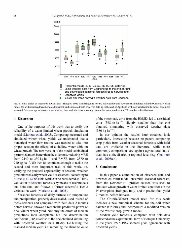
Fig. 6 shows percentiles (n 5, 10, 25, 50, 75, 90 and

95) from the distribution of the 72 replicates of wheat

yields obtained from the Demeter hindcasts for years

1977–1987 (with the exception of 1985), compared

with yields simulated using observed weather data only

(squares) and with actual yields from field experiments

(triangles).

Distributions of results obtained from downscaled

seasonal Demeter hindcasts are generally skewed, so

the comparison between simulations and field data was

carried out using central values (50th percentile, i.e.

median yields), instead of arithmetic means. The

comparison showed errors (MBE 816 kg ha�1, RMSE

1185 kg ha�1, R2 0.65**) higher than those obtained

simulating with observed weather data but close to the

standard deviation of experimental yields (1128 kg

ha�1). For comparison, results from the other percen-

tiles shown in Fig. 6 are visible in Table 1.

Table 1

Error statistics of percentile winter wheat yields simulated with

weather data up to the end of April and with downscaled multi-model

ensemble seasonal forecasts up to harvest date compared with experi-

mental yields

Percentile R2 RMSE (kg ha�1) MBE (kg ha�1)

5 0.32ns 2802 2615

10 0.37ns 2417 2195

25 0.59* 1601 1361

50 0.65** 1185 816

75 0.65** 1025 352

90 0.66** 1029 �65

95 0.67** 1107 �294

Note. Significance levels: ns (P > 0.05), *(P < 0.05), **(P < 0.01).

V. Marletto et al. / Agricultural and Forest Meteorology 147 (2007) 71–7976

Fig. 6. Final yields as measured at Cadriano (triangles, 1985 is missing due to very bad weather and poor crop), simulated with the Criteria/Wofost

model fed with observed weather data (squares), and simulated with observed data up to the end of April and with downscaled multi-model ensemble

seasonal forecasts up to harvest date (circles, box and whiskers showing percentiles computed on the 72 members distribution).

4. Discussion

One of the purposes of this work was to verify the

reliability of a water limited wheat growth simulation

model (Marletto et al., 2005). Comparing measured and

simulated winter wheat yields we understood that a

numerical water flow routine was needed to take into

proper account the effects of a shallow water table on

wheat growth. The new version of the model so obtained

performed much better than the older one, reducing MBE

from 2440 to 330 kg ha�1 and RMSE from 2570 to

710 kg ha�1. We then felt confident enough to tackle the

second and most important task of this work, i.e.

verifying the practical applicability of seasonal weather

predictions to early wheat yield assessment. According to

Morse et al. (2005) this work can be considered as Tier 3

validation of seasonal forecasts by means of user models

and field data, and follows a former successful Tier 2

verification work (Marletto et al., 2005).

Seasonal forecasts of daily surface air temperature

and precipitation, properly downscaled, used instead of

measurements and compared with field data 2 months

before harvest, showed a reasonable predictive power of

final winter wheat yield. Not only the errors of median

predictions look acceptable but the determination

coefficient (0.65) is close to the one obtained simulating

with observed weather data (0.70). De-biasing the

assessed median yield, i.e. removing the absolute value

of the systematic error from the RMSD, led to a residual

error (368 kg ha�1) slightly smaller than the one

obtained simulating with observed weather data

(380 kg ha�1).

In our opinion the results here obtained look

particularly interesting because no papers comparing

crop yields from weather seasonal forecasts with field

data are available in the literature, while more

commonly comparisons are against agricultural statis-

tical data at the district or regional level (e.g. Challinor

et al., 2005a,b).

5. Conclusions

In this paper a combination of observed data and

downscaled multi-model ensemble seasonal forecasts,

from the Demeter EU project dataset, was used to

simulate wheat growth in water limited conditions in the

Po river plain (Bologna, Italy) and to predict final yield

2 months before harvest.

The Criteria/Wofost model used for this work

includes a new numerical scheme for the soil water

balance (Criteria) and incorporates a modified version

of the Wofost crop growth model.

Median yield forecasts, compared with field data

collected at the experimental farm of Bologna University

in the years 1977–1987 showed good agreement with

observed yields.

V. Marletto et al. / Agricultural and Forest Meteorology 147 (2007) 71–79 77

In our view this result shows that wheat yields can be

reasonably well assessed 2 months before harvest using

downscaled multi-model ensemble seasonal forecasts.

There is thus a good prospect for the application of

operational seasonal forecasts to early agricultural

production prediction, even at the local scale, especially

in view of expected improvements in seasonal fore-

casting and downscaling techniques and of the possible

extension of the Criteria/Wofost model to other regions.

Acknowledgements

We are deeply indebted to Prof. Giovanni Toderi and

his research staff, who provided wheat field data. We are

also grateful to Tomaso Tonelli, who was very helpful in

software development, Gabriele Antolini, who helped

with the figures, and with Enrico Ceotto, who reviewed

an early draft of this paper. This work was carried out

within the Ph.D. thesis of Giovanna Fontana in

Agrometeorology and Ecophysiology of Agricultural

and Forest Systems, University of Sassari, coordinated

by Prof. Pietro Deidda. Financial support for this work

came from the research projects DEMETER (EU Fifth

Framework Programme, contract EVK/CT/1999/

00024) and ENSEMBLES (EU Sixth Framework

Programme, contract 505539).

Appendix A

The mono-dimensional soil water flow model used

here solves the pointwise continuity equation:

divðuÞ þ @ðWuÞ@t¼ q (1)

where u is the flux density, W the total available volume

at a point, u the fraction of W occupied by water

(volumetric water content) and q is the water input or

output. This general equation is solved adopting two

different laws to describe fluxes within the soil matrix

and fluxes on the soil surface. In the first case, it

becomes Richards’ equation:

du

dH

@H

@t¼ div½KðhÞ gradðHÞ� þ q (2)

where K(h) is the hydraulic conductivity and H the total

hydraulic head. H in turn is given by the sum of

elevation z (or gravitational component) and the hydrau-

lic matric component h = p/rw, where rw is the water

density, p the soil matric potential and t is the time. For

saturated flow, Eq. (2) reduces to the Laplace equation

for groundwater flow.

The solution of the governing equations is based on

the integrated finite difference method which consists of

the integration of the differential continuity equation

over a finite domain D, as described by de Marsily

(1986), leading to the integral equation (limited to the

one-dimensional case):Z

divðuÞ dzþZ

@ðWuÞ@t

dz ¼Z

q dz (3)

The mass balance is computed for the spatial unit D

of the model domain. Based on integral properties,

Eq. (3) can be written asZ

G D

un dSþZ

@ðWuÞ@t

dz ¼Z

q dz (4)

where GD is the surface of the computational domain D,

and n its normal unit vector. Eq. (3) can be applied over

a simulation volume within which the material proper-

ties are constant.

If the simulation domain is approximated by a three-

dimensional (or one-dimensional) grid of nodes, Eq. (4)

is equivalent to the mass balance equation for the

volume surrounding each node:

@Vi

@t¼Xn

j¼1

Qi j þ qi 8 i 6¼ j (5)

where Vi is the amount of stored water in the volume

surrounding the node, Qij the flux between the i-th and

the j-th node, and qi is the input flux at the i-th node. We

can write a system of equations for all nodes with the

unknowns being the hydraulic potentials, H.

The flux Qij is described by Darcy’s law in the finite

difference form:

Qi j ¼ �Ki jSi jðHi � H jÞ

Li j(6)

where Sij is the interfacial area between nodes i and j, Lij

the distance between the two nodes, Hi the hydraulic

potential at node i, and Kij is the internode conductivity.

The model uses the geometric mean of nodal conduc-

tivities

Ki j ¼ffiffiffiffiffiffiffiffiffiffiffiffiffiffiffiffiffiffiffiffiffiffiffiffiffiKiðHÞK jðHÞ

q; (7)

where Ki(Hi) is the hydraulic conductivity at the i-th

node. The model uses the approach proposed by van

Genuchten (1980) and Mualem (1976) for the charac-

terization of the soil water retention (SWR) and the

hydraulic conductivity (K) curves.

The model allows time and space varying boundary

conditions to each node to be specified:

V. Marletto et al. / Agricultural and Forest Meteorology 147 (2007) 71–7978

(1) n

odes with fixed hydraulic head (H = constant),

(2) n

odes set at atmospheric boundary conditions,

(3) n

odes with prescribed flux,

(4) n

odes with no flux in any given direction.

Boundary conditions of type (1) can be used to

represent various conditions, such as deep drainage at

the lower boundary, or prescribed heads given by the

presence of ponding areas, lakes or other bodies.

Atmospheric boundary conditions (2) allow prescribed

precipitation and evapotranspiration to be assigned.

Precipitation is assigned per unit area of the land surface

equivalent to the boundary area of a subsurface volume.

Regarding the coupling between surface and subsurface

flow, precipitation water is applied to the surface nodes.

The coupling between surface and subsurface nodes

occurs through the application of Richards’ equation

with different options on the calculation of the inter-

nodes conductivity.

The numerical formulation of the model produces a

strongly non-linear system, to be solved by means of

successive approximations. Every time step corre-

sponds to the computation of more approximations,

each solving a linearized system by means of a solving

method. It can be shown that the matrix produced by the

model is positive definite so the main iterative solving

methods are convergent. In particular we chose the

Gauss–Seidel algorithm, whose computational cost

seems optimal for the matrix produced by the model

(Tomei, 2005).

We faced the necessity of developing an adaptive

algorithm able to adapt time step to system condi-

tions. The main reference to monitoring the state of

the system is represented by the mass balance, that is

evaluated on the base of the mass balance ratio

(MBR). This variable is computed within the time

step as the ratio of soil water storage variation to

the sum of incoming (precipitation) and outgoing

(surface and subsurface, evaporation and transpira-

tion) flows.

MBR ¼ Dstorage

fluxin � fluxout

(7)

The two values represent the same phenomenon,

therefore in a fully conservative algorithm one should

have MBR = 1. When incoming and outgoing flows are

very low or equal the equation produces a numerical

overflow, so we prefer to use the expression:

MBR ¼ storagetþDt

storaget þ fluxin � fluxout

(8)

avoiding numerical problems, as water content never

gets to zero. The mass balance error E is then defined as

E ¼ 1�MBR (9)

that can be easily used as a parameter to evaluate the

quality of the system solution produced by every

approximation, setting a tolerance threshold below

which the balance is considered correct and the time

step is accepted.

The numerical model was implemented as a dynamic

link library (DLL) daily coupled with the Criteria/

Wofost environment. The environment inputs to the

DLL are soil data, boundary conditions (impermeable

bottom or water table depth), initial soil moisture

conditions and daily precipitation. The DLL then

computes profile water content and returns it to the

environment, which in turn simulates evaporation and

transpiration flows, root growth and above ground

biomass accumulation.

References

Ashraf, M., Zia-ul-Haq, Kahlown, M.A., 2005. Effect of shallow

groundwater table on crop water requirements and crop yields.

Agric. Water Manag. 76, 24–35.

Cantelaube, P., Terres, J.-M., 2005. Seasonal weather forecasts for

crop yield modelling in Europe. Tellus A 57 (3), 476–487.

Challinor, A.J., Wheeler, T.R., Slingo, J.M., Craufurd, P.Q., Grimes,

D.I.F., 2005a. Simulations of crop yields using ERA-40: limits to

skill and nonstationarity in weather-yield relationships. J. Appl.

Meteor. 44, 516–531.

Challinor, A.J., Slingo, J.M., Wheeler, T.R., Doblas-Reyes, F.J.,

2005b. Probabilistic simulations of crop yield over western India

using the DEMETER seasonal hindcast ensembles. Tellus A 57

(3), 498–512.

de Marsily, G., 1986. Quantitative Hydrogeology. Academic Press,

San Diego.

Feddersen, H., Andersen, U., 2005. A method for statistical down-

scaling of seasonal ensemble predictions. Tellus A 57 (3), 398–

408.

Genovese, G. 1998. The methodology, the results and the evaluation of

the MARS crop yield forecasting system, in Agrometeorological

Application for Regional Crop Monitoring and Production Assess-

ment, Account of the EU Support group on Agrometeorology

(SUGRAM), Office for Official Publications of the European

Communities, Luxembourg. Report No. EUR 17735 EN, 67–119.

Hagedorn, R., Doblas-Reyes, F.J., Palmer, T.N., 2005. The rationale

behind the success of multi-model ensembles in seasonal fore-

casting. Part I. Basic concept. Tellus A 57 (3), 219–233.

Lawless, C., Semenov, M.A., 2005. Assessing lead-time for predicting

wheat growth using a crop simulation model. Agric. For. Meteorol.

135, 302–313.

Marletto, V., 1983. Study for a climatic winter wheat yield model in

the Po river Valley. Bollett. Geofisico 6, 30–35 (in Italian).

Marletto, V., Zinoni, F., 1996. The criteria project: integration of

satellite, radar, and traditional agroclimatic data in a GIS-sup-

ported water balance modelling environment. In: Dalezios, N.R.

(Ed.), Proceedings of the International Symposium on Applied

V. Marletto et al. / Agricultural and Forest Meteorology 147 (2007) 71–79 79

Agrometeorology and Agroclimatology, COST 77, 79, 711, April

24–26, Volos, Greece, pp. 173–178.

Marletto, V., Criscuolo, L., Van Soetendael, M.R.M., 2001. Imple-

mentation of WOFOST in the framework of the CRITERIA

geographical tool. In: Proceedings of the 2nd International

Symposium on Modelling Cropping Systems, July 16–18,

European Society for Agronomy, Florence, Italy, pp. 219–

220.

Marletto, V., Zinoni, F., Criscuolo, L., Fontana, G., Marchesi, S.,

Morgillo, A., Van Soetendael, M.R.M., Ceotto, E., Andersen, U.,

2005. Evaluation of downscaled DEMETER multi-model ensem-

ble seasonal hindcasts in a northern Italy location by means of a

model of wheat growth and soil water balance. Tellus A 57 (3),

488–497.

Morse, A.P., Doblas-Reyes, F.J., Hoshen, M.B., Hagedorn, R., Palmer,

T.N., 2005. A forecast quality assessment of an end-to-end

probabilistic multi-model seasonal forecast system using a malaria

model. Tellus A 57 (3), 464–475.

Mualem, Y., 1976. A new model for predicting the hydraulic con-

ductivity of unsaturated porous media. Water Resour. Res. 12,

513–522.

Palmer, T.N., Alessandri, A., Andersen, U., Cantelaube, P., Davey, M.,

Deque, M., Dıaz, E., Doblas-Reyes, F.J., Feddersen, H., Graham,

R., Gualdi, S., Gueremy, J.-F., Hagedorn, R., Hoshen, M., Keen-

lyside, N., Latif, M., Lazar, A., Maisonnave, E., Marletto, V.,

Morse, A.P., Orfila, B., Rogel, P., Terres, J.-M., Thomson, M.C.,

2004. Development of a European multi-model ensemble system

for seasonal to inter-annual prediction (DEMETER). Bull. Am.

Meteor. Soc. 85, 853–872.

Pavan, V., Marchesi, S., Morgillo, A., Cacciamani, C., Doblas-Reyes,

F.J., 2005. Downscaling of DEMETER winter seasonal hindcasts

over Northern Italy. Tellus A 57 (3), 424–434.

Pistocchi, A., Tomei, F., 2003. Implementation of a 3D coupled

surface-subsurface numerical flow model within the framework

of the CRITERIA decision support system. In: Proceedings of the

National Congress of the Italian Association of Agrometeorology.

May 29–30, AIAM, Bologna, (in Italian), pp. 285–296.

Rossi Pisa, P., Kerschbaumer, A., 1998. Spatial and temporal repre-

sentation of watertable depth data. In ‘‘La normalizzazione dei

metodi di analisi fisica del suolo’’. I georgofili. Quaderni, III, 173–

186 (in Italian).

Thomson, M.C., Doblas-Reyes, F.J., Mason, S.J., Hagedorn, R.,

Connor, S.J., Phindela, T., Morse, A.P., Palmer, T.N., 2006.

Malaria early warnings based on seasonal climate forecasts from

multi-model ensembles. Nature 439, 576–579.

Tibaldi, S., Molteni, F., 1990. On the operational predictability of

blocking. Tellus A 42, 343–365.

Toderi, G., Rossi Pisa, P., Marotti, M., 1982. Effects of barley straw

burial on sugarbeet, wheat and barley final yields in triennial

rotation. Riv. Agron. 16, 187–196 (in Italian).

Tomei, F., 2005. Numerical analysis of hydrological processes. A

three-dimensional model of hydrological balance, Tesi Facolta di

Scienze Matematiche Fisiche e Naturali, Dipartimento di Infor-

matica, Universita di Bologna (in Italian).

van Diepen, C.A., Wolf, J., van Keulen, H., 1989. WOFOST: a

simulation model of crop production. Soil Use Manage. 5, 16–24.

van Genuchten, M.T., 1980. A closed-form equation for predicting the

hydraulic conductivity of unsaturated soils. Soil Sci. Soc. Am. J.

44, 892–898.

Ventura, F., Rossi Pisa, P., Ardizzoni, E., 2002. Temperature and

precipitation trends in Bologna (Italy) from 1952 to 1999. Atmos.

Res. 61, 203–214.

Vogel, F.A., Bange, G.A., 1999. Understanding USDA crop forecasts.

Miscellaneous Publication No. 1554, 17 pp.