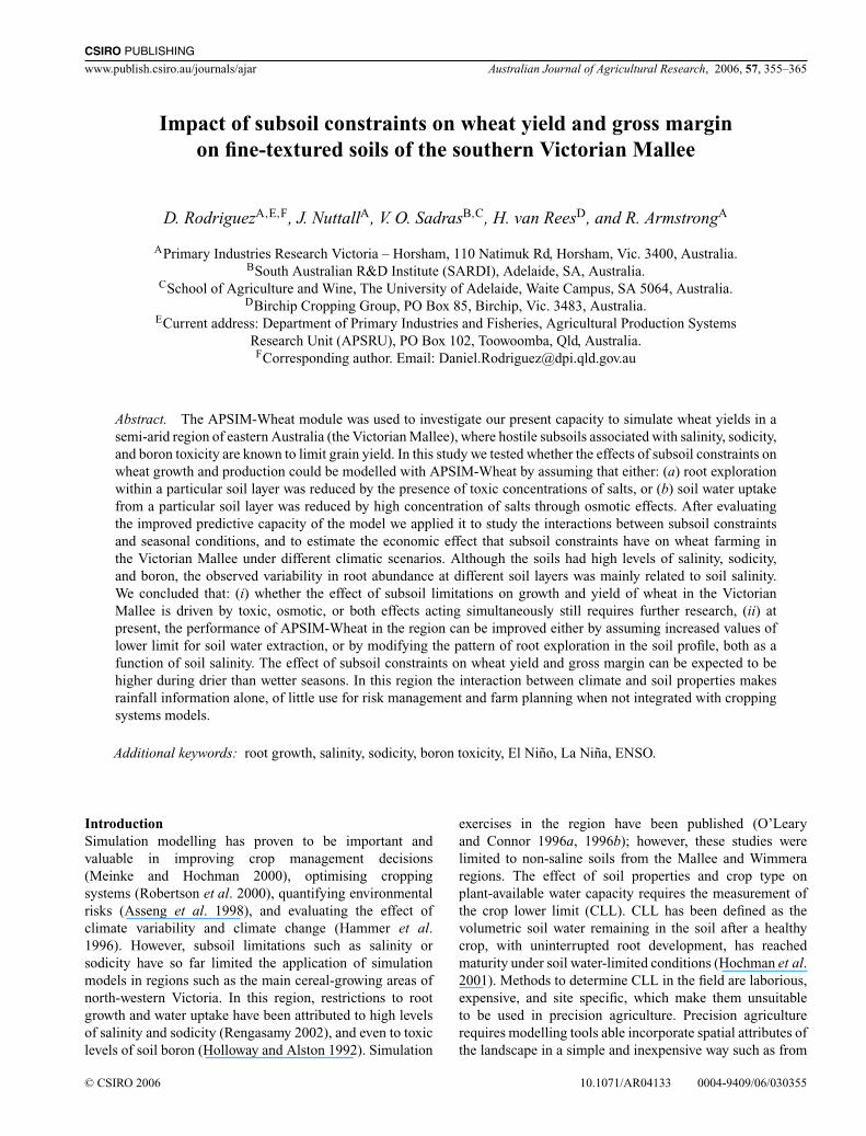
CSIRO PUBLISHING

www.publish.csiro.au/journals/ajar Australian Journal of Agricultural Research, 2006, 57, 355–365

Impact of subsoil constraints on wheat yield and gross marginon fine-textured soils of the southern Victorian Mallee

D. RodriguezA,E,F, J. NuttallA, V. O. SadrasB,C, H. van ReesD, and R. ArmstrongA

APrimary Industries Research Victoria – Horsham, 110 Natimuk Rd, Horsham, Vic. 3400, Australia.BSouth Australian R&D Institute (SARDI), Adelaide, SA, Australia.

CSchool of Agriculture and Wine, The University of Adelaide, Waite Campus, SA 5064, Australia.DBirchip Cropping Group, PO Box 85, Birchip, Vic. 3483, Australia.

ECurrent address: Department of Primary Industries and Fisheries, Agricultural Production SystemsResearch Unit (APSRU), PO Box 102, Toowoomba, Qld, Australia.FCorresponding author. Email: Daniel.Rodriguez@dpi.qld.gov.au

Abstract. The APSIM-Wheat module was used to investigate our present capacity to simulate wheat yields in asemi-arid region of eastern Australia (the Victorian Mallee), where hostile subsoils associated with salinity, sodicity,and boron toxicity are known to limit grain yield. In this study we tested whether the effects of subsoil constraints onwheat growth and production could be modelled with APSIM-Wheat by assuming that either: (a) root explorationwithin a particular soil layer was reduced by the presence of toxic concentrations of salts, or (b) soil water uptakefrom a particular soil layer was reduced by high concentration of salts through osmotic effects. After evaluatingthe improved predictive capacity of the model we applied it to study the interactions between subsoil constraintsand seasonal conditions, and to estimate the economic effect that subsoil constraints have on wheat farming inthe Victorian Mallee under different climatic scenarios. Although the soils had high levels of salinity, sodicity,and boron, the observed variability in root abundance at different soil layers was mainly related to soil salinity.We concluded that: (i) whether the effect of subsoil limitations on growth and yield of wheat in the VictorianMallee is driven by toxic, osmotic, or both effects acting simultaneously still requires further research, (ii) atpresent, the performance of APSIM-Wheat in the region can be improved either by assuming increased values oflower limit for soil water extraction, or by modifying the pattern of root exploration in the soil profile, both as afunction of soil salinity. The effect of subsoil constraints on wheat yield and gross margin can be expected to behigher during drier than wetter seasons. In this region the interaction between climate and soil properties makesrainfall information alone, of little use for risk management and farm planning when not integrated with croppingsystems models.

Additional keywords: root growth, salinity, sodicity, boron toxicity, El Nino, La Nina, ENSO.

IntroductionSimulation modelling has proven to be important andvaluable in improving crop management decisions(Meinke and Hochman 2000), optimising croppingsystems (Robertson et al. 2000), quantifying environmentalrisks (Asseng et al. 1998), and evaluating the effect ofclimate variability and climate change (Hammer et al.1996). However, subsoil limitations such as salinity orsodicity have so far limited the application of simulationmodels in regions such as the main cereal-growing areas ofnorth-western Victoria. In this region, restrictions to rootgrowth and water uptake have been attributed to high levelsof salinity and sodicity (Rengasamy 2002), and even to toxiclevels of soil boron (Holloway and Alston 1992). Simulation

exercises in the region have been published (O’Learyand Connor 1996a, 1996b); however, these studies werelimited to non-saline soils from the Mallee and Wimmeraregions. The effect of soil properties and crop type onplant-available water capacity requires the measurement ofthe crop lower limit (CLL). CLL has been defined as thevolumetric soil water remaining in the soil after a healthycrop, with uninterrupted root development, has reachedmaturity under soil water-limited conditions (Hochman et al.2001). Methods to determine CLL in the field are laborious,expensive, and site specific, which make them unsuitableto be used in precision agriculture. Precision agriculturerequires modelling tools able incorporate spatial attributes ofthe landscape in a simple and inexpensive way such as from

© CSIRO 2006 10.1071/AR04133 0004-9409/06/030355

356 Australian Journal of Agricultural Research D. Rodriguez et al.

the determination of subsoil salinity from EM38 surveys(O’Leary et al. 2004). However, before this can be achieveda better understanding of the mechanisms linking subsoilconstraints and crop growth and yield in simulation modelsis required. In this study we aim to: (i) test whether the effectsof subsoil constraints on wheat growth and production canbe modelled with APSIM-Wheat by assuming that either(a) root exploration within a particular soil layer is reducedby the presence of toxic concentrations of salts, or (b) soilwater uptake from a particular soil layer is reduced by highconcentration of salts through osmotic effects; (ii) study theimportance of the interactions between subsoil constraintsand seasonal conditions; and (iii) quantify the economiceffect of both subsoil constraints and climate variability inthe Victorian Mallee of Victoria.

MethodsField experiments

Data sets from wheat (Triticum aestivum L.) crops grown in on-farmexperiments in the southern Mallee of Victoria, Australia, were obtainedfor the cropping seasons 1993, 1994, and 1999. During the first 2 years(Expt 1), soil and crop data were collected from 2 commercial crops atBrim (36.07◦S, 142.42◦E) and Birchip (35.98◦S, 142.92◦E), and during1999 (Expt 2), 16 sites were randomly selected from 150 surveyedsites (Nuttall et al. 2003a) covering an area of 3600 km2 in the Birchipdistrict. The soils in the region are mainly Calcarosols (Nuttall et al.2003a), and the long-term (1957–2002) average seasonal (1 April–1 November) rainfall is 257 mm.

Field Expt 1

During the 1993 and 1994 cropping seasons, 2 wheat fields (Triticumaestivum L. cv. Frame) from the Brim and Birchip areas were sampledto determine soil water, N-NO3 (mg/kg), organic carbon (%), electricconductivity (EC, dS/m), bulk density (g/cm3), and pH at 0–0.1,0.1–0.6, and 0.6–1 m depths. Crop data included date of anthesis,maximum rooting depth, grain yield, and above-ground biomass. Aftersowing the wheat crop in autumn 1993 the soil water content of thedifferent soil layers was measured at about monthly intervals using aneutron moisture meter (Model 503, Campbell Pacific Nuclear Crop,Martinez, CA). Surface-layer soil water (0–0.25 m) was measuredgravimetrically. Results are averages of 3–5 replications withineach paddock.

Field Expt 2

Soil and crop data were collected from the Birchip district of Victoria,Australia (Nuttall et al. 2003a). The data set consisted of soil and cropcharacteristics determined in transects of 10 points at 15 locations,i.e. 150 sites, within a radius of c. 30 km around Birchip, collectedduring the 1999 season. At each site the following soil variableswere determined at different depths in the soil profile: soil boron(mg B/kg soil), EC (dS/m), exchangeable sodium (ESP, %), N-NO3

(mg/kg), volumetric soil water content at sowing, volumetric soilwater content at wilting point (WP), and bulk density. Among others,crop variables included layered root dry weight at anthesis, and finalgrain yield.

Simulation Expt 1

The Agricultural Production Systems Simulator (APSIM) (McCownet al. 1996) allows the simulation of diverse crops and croppingsystems targetting issues such as land degradation (Asseng et al.2001), crop rotation (Carberry et al. 1996), cropping strategies

(Robertson et al. 2000), and management alternatives (Goyne et al.1996). APSIM-Wheat (APSIM version 2.1 patch 2) has been testedagainst field studies in different regions of Australia and locally for thisstudy. In this exercise we used the model APSIM-Wheat parameterisedwith modules SOILN2, SOILWAT2, and RESIDUE2. The phenologyparameters of the model were calibrated for the wheat crop cv. Frameusing an independent data set provided by Dr R. Flood (unpublisheddata). Values of soil water content at saturation (SAT) were calculatedfrom values of bulk density (Dalgliesh and Foale 1998), values ofdrainage upper limit (DUL) were derived from a relationship betweenSAT and DUL determined from wet ponds in soils of the Mallee region,and soil water lower limits (LL) were taken as soil water contentsdetermined in the laboratory at −15 kPa (WP). Wheat yields weresimulated assuming: (i) the observed root distribution within the soilprofile at each site and measured values of LL15 as inputs to themodel (Hypothesis A), (ii) ignoring the presence of subsoil constraintsand using measured values of LL15 (control), (iii) calculating theroot soil profile distribution from a function relating root distributionand EC (dS/m) (Hypothesis A), and (iv) calculating the value ofthe crop lower limit (parameter ll in APSIM) for each soil layer,as a function of the EC (dS/m) as proposed by Sadras et al. (2003)(Hypothesis B). Within APSIM the effects of EC on root distributionwere incorporated by modifying the value of the parameter ‘xf ’, i.e. rootexploration factor for each soil layer. The agreement between observedand simulated results was evaluated by comparing the coefficient ofdetermination, root mean squared error, and by desegregating the meansquared error following the methodology proposed by Kobayashi andSalam (2000).

Simulation Expt 2

To study the interactions between subsoil constraints and seasonalconditions on grain yield and economic return at Birchip, we used croplower limits (parameter ll in APSIM) calculated as a function of EC(dS/m) as in Sadras et al. (2003). Historical climate data for the period1900–2002 years (Birchip Post Office, station no. 77007), were obtainedfrom the Silo Patched Point Data Set (http://www.bom.gov.au/silo).Simulated treatments included 3 levels of soil salinity, i.e. low(decile 1), median (decile 5), and high (decile 9) (see Fig. 1a).Simulation outputs are presented for all the simulated years andfor those years defined as El Nino years and La Nina years (asin http://www.longpaddock.qld.gov.au). Gross margin in A$/ha wasestimated as the product of yield and price minus variable costs;we did not take into account fixed costs. Variable costs, includingfertilisers, were set at A$158.76/ha, and included the cost of contractingmachinery works (including harvest), seed, and chemicals. Grain pricewas calculated depending on grain quality following the AustralianWheat Board standards. Initial conditions for model simulations werereset every 1 January to 10% of plant-available water, 50 kg N/ha,and 1000 kg/ha of canola residues from previous crop. Every year,50 kg N/ha were applied at sowing.

Results

Subsoil constraints

Figure 1 shows the main chemical and physical characteristicsof the sites under study. In general terms the concentrationand levels of variability in soil salinity, sodicity, and boronincreased with soil depth, whereas the values of wiltingpoint varied little. The ‘regional’ variability, i.e. coefficient ofvariation, %, for each of these parameters at each of the soildepths was greatest for boron in the upper layers (0–0.4 m),and for salinity in the deeper layers (0.4–1 m) (Table 1).Interestingly the coefficients of variation for soil sodicity

Subsoil constraints, wheat yield, and gross margin Australian Journal of Agricultural Research 357

0.0

0.1

0.2

0.3

0.4

0.5

0.6

0.7

0.8

0.9

1.0

0 1 2 3 4 5

EC (dS/m)

0–0.2 m

0.2–0.4 m

0.4–0.6 m

0.6–1 m

Critical value = 0.8

(a)

0 10 20 30 40 50

ESP (%)

0–0.2 m0.2–0.4 m0.4–0.6 m0.6–1 m

Critical value = 19

(b)

0.0

0.1

0.2

0.3

0.4

0.5

0.6

0.7

0.8

0.9

1.0

0 20 40 60

Boron (mg/kg)

Cum

ulat

ive

prob

abili

ty

0–0.2 m0.2–0.4 m0.4–0.6 m0.6–1 m

Critical value = 24

(c)

0 10 20 30 40

WP (v/v)

0–0.2 m0.2–0.4 m0.4–0.6 m0.6–1 m

(d )

Fig. 1. Cumulative probability distribution of (a) soil salinity, EC (dS/m); (b) (%) exchangeable sodiumpercentage, ESP; (c) soil boron; and (d ) volumetric soil water content at −15 kPa (WP), at 0–0.2, 0.2–0.4,0.4–0.6, and 0.6–1 m depths from 150 sites around Birchip. Vertical lines in a, b, and c indicate criticalthreshold values for grain yield. After Nuttall et al. (2003a).

Table 1. Coefficients of variation (%) for salinity (EC),exchangeable sodium percentage (ESP), boron (B), cation exchangecapacity (CEC), and soil water −15 kPa (WP), at differentdepths, observed in soil samples from the Birchip region (after

Nuttall et al. 2003a)

Soil layer (m) EC ESP B CEC WP

0–0.2 55.0 67.8 94.1 28.5 25.90.2–0.4 59.4 54.2 79.5 19.3 24.00.4–0.6 68.8 39.8 58.5 17.9 22.40.6–1 54.8 33.7 40.0 17.1 20.0

were highly correlated with the coefficients of variationfor boron, cation exchange capacity, and soil lower limit(Table 2), but not with the coefficients of variation for soilsalinity.

Frequency distributions of key soil chemical constraintswere compared with the critical values derived by Nuttallet al. (2003b). In more than 50% of the sites, salinity washigher than the critical value of 0.8 dS/m at depths below0.6 m. In about 50% of the sites, sodicity and boron were

Table 2. Correlation matrix for the coefficients of variation acrossdifferent soil chemical and physical properties

Soil salinity (EC), exchangeable sodium percentage (ESP), boron (B),cation exchange capacity (CEC), and soil water –15 kPa (WP) at

different depths, observed in soil samples from the Birchip region

EC ESP B CEC

EC 1ESP −0.32 1B −0.16 0.98 1CEC −0.42 0.91 0.83 1WP −0.094 0.97 0.99 0.85

above the critical values of 19% and 24 mg/kg at depthsbelow 0.6 m.

Simulation Expt 1

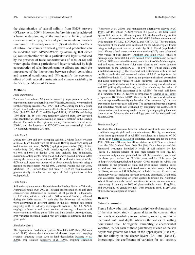
A soil rooting distribution factor, i.e. relative root massdensity, was calculated from the measured values of rootmass in each layer, relative to the root mass density in theupper layer (0–0.1 m) at each of the 150 sites (Fig. 2). The

358 Australian Journal of Agricultural Research D. Rodriguez et al.

0

0.1

0.2

0.3

0.4

0.5

0.6

0.7

0.8

0.9

1

0 0.5 1 1.5 2 2.5

Relative root mass density

Pro

babi

lity

of e

xede

nce

0–0.1 m

0.1–0.2 m

0.2–0.4 m

0.4–0.6 m

0.6–1.0 m

Fig. 2. Probability distribution for the root mass density in differentsoil layers relative to that in the 0–0.1 m layer for 150 sites aroundBirchip. After Nuttall et al. (2003b).

median root distribution factor (RDF) for the layer 0.1–0.2 mwas 0.74, for the layer 0.2–0.4 m was 0.47, for the layer0.4–0.6 m was 0.41, and for the layer 0.6–1 m was 0.12. Toeliminate the effect of declining root mass density with depth,a standardised root expansion factor was derived for eachsoil layer. This factor was calculated relative to the RDFvalues observed in each layer at the site that produced thehighest grain yield, i.e. 6 t/ha. At this site the values of salinity,sodicity, and boron were low in all soil layers.

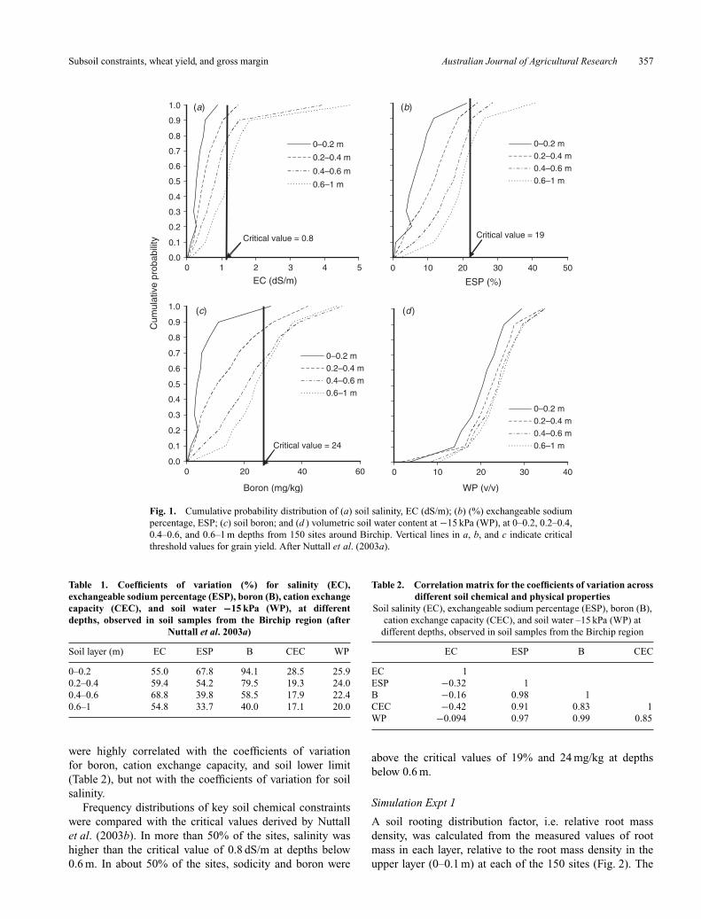
The soil characteristic that best explained the observedvariability in the root expansion factor among soil layersand sites was soil salinity. The values of the root expansionfactor in the 0.4–1 m layer were inversely correlated withEC (r = –0.59), soil sodicity (r = –0.53), and soil boron(r = –0.47). In this exercise we assumed that soil salinitywas the main limiting factor for soil root exploration atdepth. From the relationship shown in Fig. 3, we assumedthat the root expansion factor had a value of 1 for EC below0.68 dS/m, and that it decreased hyperbolically to 0 at valuesof EC higher than 0.68 dS/m (Eqn 1):

if EC < 0.68, Root expansion factor = 1

if EC ≥ 0.68, Root expansion factor = 2.06

(1 + 2 · EC)− 0.35 (1)

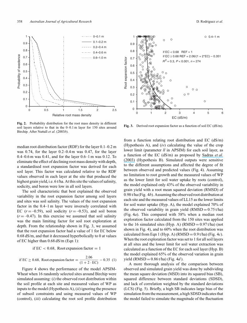
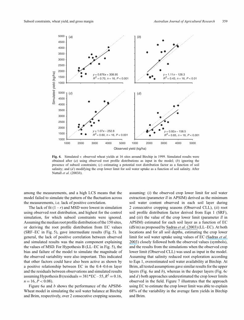
Figure 4 shows the performance of the model APSIM-Wheat when 16 randomly selected sites around Birchip weresimulated assuming: (i) the observed root distribution withinthe soil profile at each site and measured values of WP asinputs to the model (Hypothesis A), (ii) ignoring the presenceof subsoil constraints and using measured values of WP(control), (iii) calculating the root soil profile distribution

0

0.1

0.2

0.3

0.4

0.5

0.6

0.7

0.8

0.9

1

0 1 2 3 4 5 6

EC (dS/m)

Roo

t exp

ansi

on fa

ctor

0.4–1 m

if EC < 0.68 REF = 1if EC ≥ 0.68 REF = 2.06/(1 + 2*EC) – 0.351

R 2 = 0.3, P < 0.001, n = 274

Fig. 3. Derived root expansion factor as a function of soil EC (dS/m).

from a function relating root distribution and EC (dS/m)(Hypothesis A), and (iv) calculating the value of the croplower limit (parameter ll in APSIM) for each soil layer, asa function of the EC (dS/m) as proposed by Sadras et al.(2003) (Hypothesis B). Simulated outputs were sensitiveto the different assumptions and affected the degree of fitbetween observed and predicted values (Fig. 4). Assumingno limitation to root growth and the measured values of WPas the lower limit for soil water uptake by roots (control),the model explained only 43% of the observed variability ingrain yield with a root mean squared deviation (RMSD) of0.98 t/ha (Fig. 4b). Assuming the observed root distribution ateach site and the measured values of LL15 as the lower limitsfor soil water uptake (Hyp. A), the model explained 70% ofthe observed variability in grain yield (RMSD = 0.75 t/ha)(Fig. 4a). This compared with 58% when a median rootexploration factor calculated from the 150 sites was appliedto the 16 simulated sites (Hyp. A) (RMSD = 0.97 t/ha) (notshown in Fig. 4), and to 60% when the root distribution wascalculated from Eqn 1 (Hyp. A) (RMSD = 0.9 t/ha) (Fig. 4c).When the root exploration factor was set to 1 for all soil layersat all sites and the lower limit for soil water extraction wascalculated as a function of the EC for each soil layer (Hyp. B)the model explained 65% of the observed variation in grainyield (RMSD = 0.86 t/ha) (Fig. 4d ).

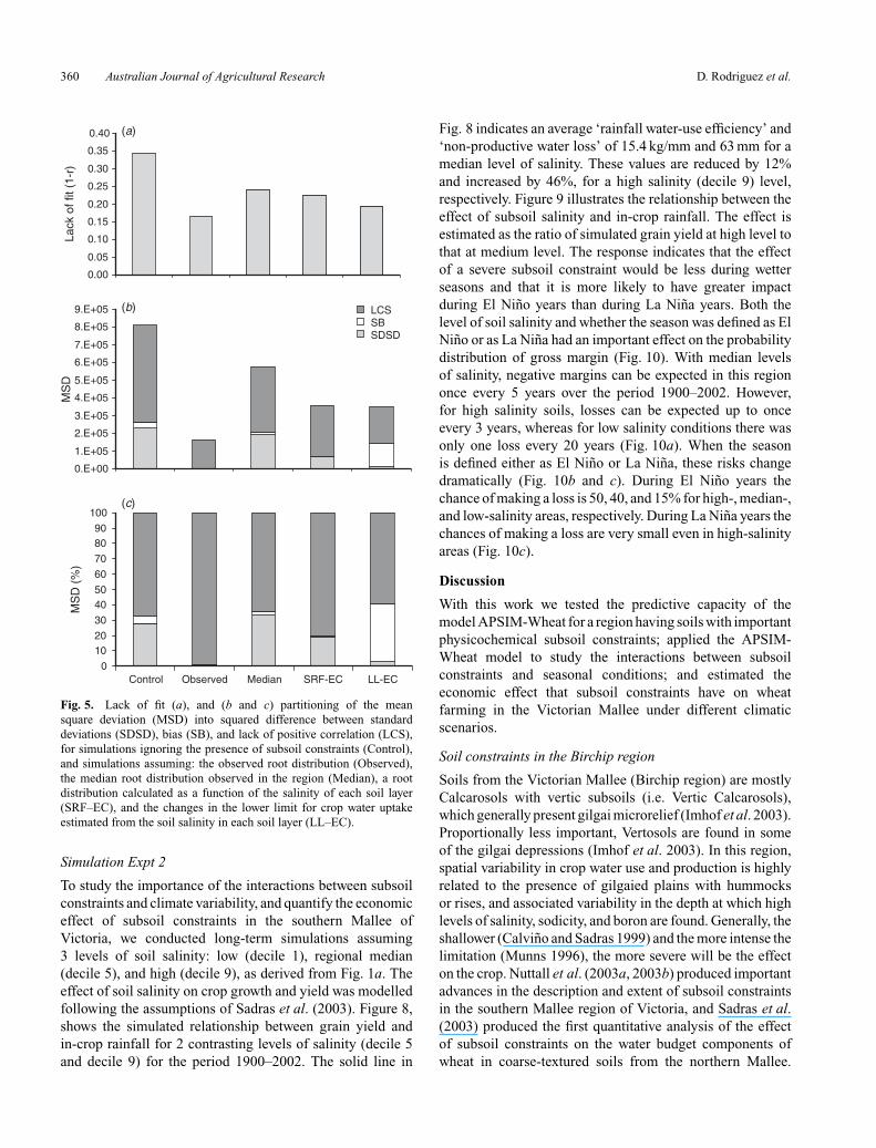
A more thorough analysis of the comparison betweenobserved and simulated grain yield was done by subdividingthe mean square deviation (MSD) into its squared bias (SB),squared difference between standard deviations (SDSD),and lack of correlation weighted by the standard deviations(LCS) (Fig. 5). Briefly, a high SB indicates large bias of thesimulation from the measurement, a high SDSD indicates thatthe model failed to simulate the magnitude of the fluctuation

Subsoil constraints, wheat yield, and gross margin Australian Journal of Agricultural Research 359

y = 0.876x + 308.95R 2 = 0.70, n = 16, P < 0.001

1000

1500

2000

2500

3000

3500

4000

4500

5000 (a)

y = 1.11x – 128.3R 2 = 0.43, n = 16, P < 0.01

(b)

y = 1.07x – 252.8R 2 = 0.60, n = 16, P < 0.001

1000

1500

2000

2500

3000

3500

4000

4500

5000

1000 2000 3000 4000 5000

Observed yield (kg/ha)

Sim

ulat

ed y

ield

(kg

/ha)

(c)

y = 0.92x – 158.5R 2 = 0.65, n = 16, P < 0.001

1000 2000 3000 4000 5000

(d)

Fig. 4. Simulated v. observed wheat yields at 16 sites around Birchip in 1999. Simulated results wereobtained after (a) using observed root profile distributions as input in the model; (b) ignoring thepresence of subsoil constraints; (c) estimating a potential root distribution factor as a function of soilsalinity; and (d ) modifying the crop lower limit for soil water uptake as a function of soil salinity. AfterNuttall et al. (2003b).

among the measurements, and a high LCS means that themodel failed to simulate the pattern of the fluctuation acrossthe measurements, i.e. lack of positive correlation.

The lack of fit (1 – r) and MSD were lowest in simulationusing observed root distribution, and highest for the controlsimulation, for which subsoil constraints were ignored.Assuming the median root profile distribution of the 150 sites,or deriving the root profile distribution from EC values(SRF–EC in Fig. 5), gave intermediate results (Fig. 5). Ingeneral, the lack of positive correlation between observedand simulated results was the main component explainingthe values of MSD. For Hypothesis B (LL–EC in Fig. 5), thebias and failure of the model to simulate the magnitude ofthe observed variability were also important. This indicatedthat other factors could have also been active as shown bya positive relationship between EC in the 0.4–0.6 m layerand the residuals between observations and simulated resultsassuming Hypothesis B (residuals = 381*EC – 55, R2 = 0.16,n = 16, P < 0.08).

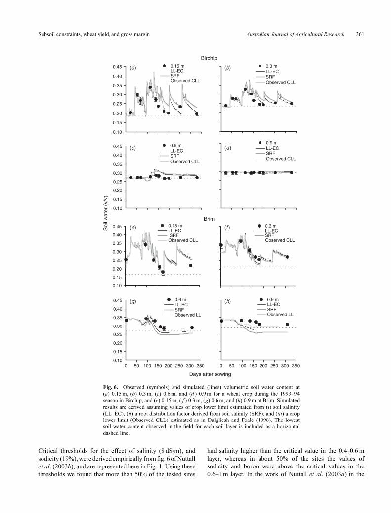
Figure 6a and b shows the performance of the APSIM-Wheat model in simulating the soil water balance at Birchipand Brim, respectively, over 2 consecutive cropping seasons,

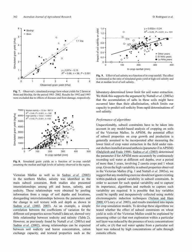
assuming: (i) the observed crop lower limit for soil waterextraction (parameter ll in APSIM) derived as the minimumsoil water content observed in each soil layer during2 consecutive cropping seasons (Observed CLL), (ii) rootsoil profile distribution factor derived from Eqn 1 (SRF),and (iii) the value of the crop lower limit (parameter ll inAPSIM) estimated for each soil layer as a function of EC(dS/m) as proposed by Sadras et al. (2003) (LL–EC). At bothlocations and for all soil depths, estimating the crop lowerlimit for soil water uptake using values of EC (Sadras et al.2003) closely followed both the observed values (symbols),and the results from the simulations when the observed croplower limit (Observed CLL) was used as input in the model.Assuming that salinity reduced root exploration accordingto Eqn 1, overestimated soil water availability at Birchip. AtBrim, all tested assumptions gave similar results for the upperlayers (Fig. 6a and b), whereas in the deeper layers (Fig. 6cand d ) both approaches underestimated the crop lower limitsobserved in the field. Figure 7 illustrates that the approachusing EC to estimate the crop lower limit was able to explain68% of the variability in the average farm yields in Birchipand Brim.

360 Australian Journal of Agricultural Research D. Rodriguez et al.

0

1020

30

4050

60

70

8090

100

Control Observed Median SRF-EC LL-EC

MS

D (

%)

(c)

0.E+00

1.E+05

2.E+05

3.E+05

4.E+05

5.E+05

6.E+05

7.E+05

8.E+05

9.E+05

MS

D

LCSSBSDSD

(b)

0.00

0.05

0.10

0.15

0.20

0.25

0.30

0.35

0.40

Lack

of f

it (1

-r)

(a)

Fig. 5. Lack of fit (a), and (b and c) partitioning of the meansquare deviation (MSD) into squared difference between standarddeviations (SDSD), bias (SB), and lack of positive correlation (LCS),for simulations ignoring the presence of subsoil constraints (Control),and simulations assuming: the observed root distribution (Observed),the median root distribution observed in the region (Median), a rootdistribution calculated as a function of the salinity of each soil layer(SRF–EC), and the changes in the lower limit for crop water uptakeestimated from the soil salinity in each soil layer (LL–EC).

Simulation Expt 2

To study the importance of the interactions between subsoilconstraints and climate variability, and quantify the economiceffect of subsoil constraints in the southern Mallee ofVictoria, we conducted long-term simulations assuming3 levels of soil salinity: low (decile 1), regional median(decile 5), and high (decile 9), as derived from Fig. 1a. Theeffect of soil salinity on crop growth and yield was modelledfollowing the assumptions of Sadras et al. (2003). Figure 8,shows the simulated relationship between grain yield andin-crop rainfall for 2 contrasting levels of salinity (decile 5and decile 9) for the period 1900–2002. The solid line in

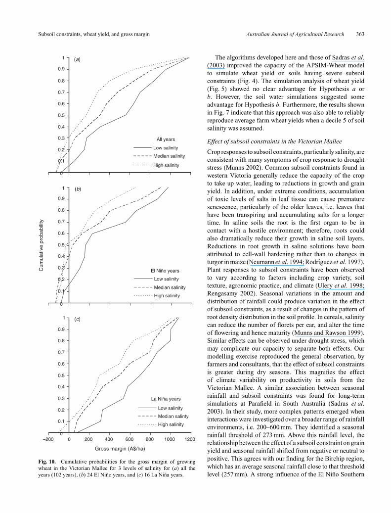
Fig. 8 indicates an average ‘rainfall water-use efficiency’ and‘non-productive water loss’ of 15.4 kg/mm and 63 mm for amedian level of salinity. These values are reduced by 12%and increased by 46%, for a high salinity (decile 9) level,respectively. Figure 9 illustrates the relationship between theeffect of subsoil salinity and in-crop rainfall. The effect isestimated as the ratio of simulated grain yield at high level tothat at medium level. The response indicates that the effectof a severe subsoil constraint would be less during wetterseasons and that it is more likely to have greater impactduring El Nino years than during La Nina years. Both thelevel of soil salinity and whether the season was defined as ElNino or as La Nina had an important effect on the probabilitydistribution of gross margin (Fig. 10). With median levelsof salinity, negative margins can be expected in this regiononce every 5 years over the period 1900–2002. However,for high salinity soils, losses can be expected up to onceevery 3 years, whereas for low salinity conditions there wasonly one loss every 20 years (Fig. 10a). When the seasonis defined either as El Nino or La Nina, these risks changedramatically (Fig. 10b and c). During El Nino years thechance of making a loss is 50, 40, and 15% for high-, median-,and low-salinity areas, respectively. During La Nina years thechances of making a loss are very small even in high-salinityareas (Fig. 10c).

Discussion

With this work we tested the predictive capacity of themodel APSIM-Wheat for a region having soils with importantphysicochemical subsoil constraints; applied the APSIM-Wheat model to study the interactions between subsoilconstraints and seasonal conditions; and estimated theeconomic effect that subsoil constraints have on wheatfarming in the Victorian Mallee under different climaticscenarios.

Soil constraints in the Birchip region

Soils from the Victorian Mallee (Birchip region) are mostlyCalcarosols with vertic subsoils (i.e. Vertic Calcarosols),which generally present gilgai microrelief (Imhof et al. 2003).Proportionally less important, Vertosols are found in someof the gilgai depressions (Imhof et al. 2003). In this region,spatial variability in crop water use and production is highlyrelated to the presence of gilgaied plains with hummocksor rises, and associated variability in the depth at which highlevels of salinity, sodicity, and boron are found. Generally, theshallower (Calvino and Sadras 1999) and the more intense thelimitation (Munns 1996), the more severe will be the effecton the crop. Nuttall et al. (2003a, 2003b) produced importantadvances in the description and extent of subsoil constraintsin the southern Mallee region of Victoria, and Sadras et al.(2003) produced the first quantitative analysis of the effectof subsoil constraints on the water budget components ofwheat in coarse-textured soils from the northern Mallee.

Subsoil constraints, wheat yield, and gross margin Australian Journal of Agricultural Research 361

0.10

0.15

0.20

0.25

0.30

0.35

0.40

0.45 0.15 mLL-ECSRFObserved CLL

(a) 0.3 mLL-ECSRFObserved CLL

0.10

0.15

0.20

0.25

0.30

0.35

0.40

0.45 0.6 mLL-ECSRFObserved CLL

0.9 mLL-ECSRFObserved CLL

0.10

0.15

0.20

0.25

0.30

0.35

0.40

0.45 0.15 mLL-EC SRFObserved CLL

0.3 mLL-ECSRFObserved CLL

0.10

0.15

0.20

0.25

0.30

0.35

0.40

0.45

0 50 100 150 200 250 300 350

Days after sowing

Soi

l wat

er (

v/v)

0.6 mLL-ECSRFObserved LL

0 50 100 150 200 250 300 350

0.9 mLL-ECSRFObserved LL

(d )(c)

(b)

(e)

(h)(g)

(f )

Brim

Birchip

Fig. 6. Observed (symbols) and simulated (lines) volumetric soil water content at(a) 0.15 m, (b) 0.3 m, (c) 0.6 m, and (d ) 0.9 m for a wheat crop during the 1993–94season in Birchip, and (e) 0.15 m, ( f ) 0.3 m, (g) 0.6 m, and (h) 0.9 m at Brim. Simulatedresults are derived assuming values of crop lower limit estimated from (i) soil salinity(LL–EC), (ii) a root distribution factor derived from soil salinity (SRF), and (iii) a croplower limit (Observed CLL) estimated as in Dalgliesh and Foale (1998). The lowestsoil water content observed in the field for each soil layer is included as a horizontaldashed line.

Critical thresholds for the effect of salinity (8 dS/m), andsodicity (19%), were derived empirically from fig. 6 of Nuttallet al. (2003b), and are represented here in Fig. 1. Using thesethresholds we found that more than 50% of the tested sites

had salinity higher than the critical value in the 0.4–0.6 mlayer, whereas in about 50% of the sites the values ofsodicity and boron were above the critical values in the0.6–1 m layer. In the work of Nuttall et al. (2003a) in the

362 Australian Journal of Agricultural Research D. Rodriguez et al.

y = 0.97x – 0.15R2 = 0.68, n = 36, P < 0.001

0

1

2

3

4

5

6

0 1 2 3 4 5 6

Observed grain yield (t/ha)

Sim

ulat

ed g

rain

yie

ld (

t/ha)

Birchip

Brim

1:1 line

Fig. 7. Observed v. simulated average farm wheat yields for 2 farms atBrim and Birchip, for the period 1983–2002. Results for 1992 and 1993were excluded due to effects of diseases and frost damage, respectively.

0

1000

2000

3000

4000

5000

6000

7000

0 100 200 300 400 500

In crop rainfall (mm)

Sim

ulat

ed g

rain

yie

ld (

kg/h

a)

Median salinity = 15.4x – 967.0

R2 = 0.45, P < 0.001, n = 102

High salinity = 13.5x – 1239.2

R 2 = 0.43, P < 0.001, n =102

Fig. 8. Simulated grain yields as a function of in-crop rainfallassuming the median and high levels of salinity observed in the region.

Victorian Mallee as well as in Sadras et al. (2003)in the northern Mallee, salinity was identified as themain subsoil constraint. Both studies also presentedinterrelationships among pH and boron, salinity, andsodicity. These relationships were obtained by poolinginformation from a range of soil depths and locations,disregarding interrelationships between the parameters andthe change in soil texture with soil depth as shown inSadras et al. (2002, 2003). As an example, a simplecorrelation between the coefficients of variation for thedifferent soil properties across Nuttall’s data set, showed verylittle relationship between sodicity and salinity (Table 2).However, as previously found by Nuttall et al. (2003a) andSadras et al. (2002), strong relationships can be expectedbetween soil sodicity and boron concentration, cationexchange capacity, and textural properties such as the

0

0.2

0.4

0.6

0.8

1

1.2

1.4

0 100 200 300 400

In crop rainfall (mm)

Impa

ct o

f soi

l sal

inity

on

yiel

d

Other yearsEl Niño yearsLa Niña years

y = 0.002x + 0.24

R 2 = 0.25, P < 0.01, n = 101

Fig. 9. Effect of soil salinity as a function of in-crop rainfall. The effectis estimated as the ratio of simulated grain yield at high soil salinity andthat at median level of soil salinity.

laboratory-determined lower limit for soil water extraction.We think this supports the argument by Nuttall et al. (2003a)that the accumulation of salts in these soils might haveoccurred later than their alkalinisation, which limits ourcapacity to predict soil sodicity from rapid determinations ofsoil salinity.

Performance of algorithms

Unquestionably, subsoil constraints have to be taken intoaccount in any model-based analysis of cropping on soilsof the Victorian Mallee. In APSIM, the potential effectof subsoil properties on crop growth and production isgenerally assumed to be incorporated after measuring thelower limit of crop water extraction in the field under rain-out shelters installed around anthesis (parameter ll in APSIM)(Dalgliesh and Foale 1998). Sadras et al. (2003) determinedthe parameter ll for APSIM more accurately by continuouslyrecording soil water at different soil depths, over a periodof more than 3 years, involving 2 canola crops and 1 wheatcrop. Given the high variability in subsoil properties observedin the Victorian Mallee (Fig. 1 and Nuttall et al. 2003a), wesuggest that any modelling exercise should not ignore existingwithin-paddock spatial variability in subsoil constraints. Inorder to account for such spatial variability and to captureits importance, algorithms and methods to capture suchvariability are required. It is possible that key variablescould be rapidly and inexpensively collected using mobileelectromagnetic induction techniques (Nelson and Ham2000; O’Leary et al. 2003), and results translated into inputsfor crop simulation models. To develop these algorithms wetested whether the effect of subsoil constraints on wheatyield in soils of the Victorian Mallee could be explained byassuming either (a) that root exploration within a particularsoil layer was reduced by the presence of toxic concentrationsof salts; or (b) that soil water uptake from a particular soillayer was reduced by high concentrations of salts throughosmotic effects.

Subsoil constraints, wheat yield, and gross margin Australian Journal of Agricultural Research 363

0

0.1

0.2

0.3

0.4

0.5

0.6

0.7

0.8

0.9

1

Low salinity

Median salinity

High salinity

All years

(a)

0

0.1

0.2

0.3

0.4

0.5

0.6

0.7

0.8

0.9

1

Cum

ulat

ive

prob

abili

ty

Low salinity

Median salinity

High salinity

El Niño years

(b)

0

0.1

0.2

0.3

0.4

0.5

0.6

0.7

0.8

0.9

1

–200 0 200 400 600 800 1000 1200

Gross margin (A$/ha)

Low salinity

Median salinty

High salinity

La Niña years

(c)

Fig. 10. Cumulative probabilities for the gross margin of growingwheat in the Victorian Mallee for 3 levels of salinity for (a) all theyears (102 years), (b) 24 El Nino years, and (c) 16 La Nina years.

The algorithms developed here and those of Sadras et al.(2003) improved the capacity of the APSIM-Wheat modelto simulate wheat yield on soils having severe subsoilconstraints (Fig. 4). The simulation analysis of wheat yield(Fig. 5) showed no clear advantage for Hypothesis a orb. However, the soil water simulations suggested someadvantage for Hypothesis b. Furthermore, the results shownin Fig. 7 indicate that this approach was also able to reliablyreproduce average farm wheat yields when a decile 5 of soilsalinity was assumed.

Effect of subsoil constraints in the Victorian Mallee

Crop responses to subsoil constraints, particularly salinity, areconsistent with many symptoms of crop response to droughtstress (Munns 2002). Common subsoil constraints found inwestern Victoria generally reduce the capacity of the cropto take up water, leading to reductions in growth and grainyield. In addition, under extreme conditions, accumulationof toxic levels of salts in leaf tissue can cause prematuresenescence, particularly of the older leaves, i.e. leaves thathave been transpiring and accumulating salts for a longertime. In saline soils the root is the first organ to be incontact with a hostile environment; therefore, roots couldalso dramatically reduce their growth in saline soil layers.Reductions in root growth in saline solutions have beenattributed to cell-wall hardening rather than to changes inturgor in maize (Neumann et al. 1994; Rodrıguez et al. 1997).Plant responses to subsoil constraints have been observedto vary according to factors including crop variety, soiltexture, agronomic practice, and climate (Ulery et al. 1998;Rengasamy 2002). Seasonal variations in the amount anddistribution of rainfall could produce variation in the effectof subsoil constraints, as a result of changes in the pattern ofroot density distribution in the soil profile. In cereals, salinitycan reduce the number of florets per ear, and alter the timeof flowering and hence maturity (Munns and Rawson 1999).Similar effects can be observed under drought stress, whichmay complicate our capacity to separate both effects. Ourmodelling exercise reproduced the general observation, byfarmers and consultants, that the effect of subsoil constraintsis greater during dry seasons. This magnifies the effectof climate variability on productivity in soils from theVictorian Mallee. A similar association between seasonalrainfall and subsoil constraints was found for long-termsimulations at Parafield in South Australia (Sadras et al.2003). In their study, more complex patterns emerged wheninteractions were investigated over a broader range of rainfallenvironments, i.e. 200–600 mm. They identified a seasonalrainfall threshold of 273 mm. Above this rainfall level, therelationship between the effect of a subsoil constraint on grainyield and seasonal rainfall shifted from negative or neutral topositive. This agrees with our finding for the Birchip region,which has an average seasonal rainfall close to that thresholdlevel (257 mm). A strong influence of the El Nino Southern

364 Australian Journal of Agricultural Research D. Rodriguez et al.

Oscillation was also observed on the effect of soil salinitylevel on grain yield (Fig. 9) and gross margin (Fig. 10).The more frequent occurrence of drier seasons during ElNino years increased the chance of low or negative grossmargins, whereas the more frequent wetter seasons during LaNina years significantly decreased this chance. These resultsindicate an important interaction between seasonal conditionsand the intensity of the subsoil constraints.

Conclusions

On soils having subsoil constraints, climate variability andsoil properties interact in such a way that rainfall informationalone will provide an incomplete picture of the effect ofclimate variability on yield. This highlights the importanceof the integration of soil properties and climate conditionswith cropping systems models for risk management and farmplanning. Simulation exercises in the Victorian Mallee shouldaccount for the presence of subsoil constraints. Here we haveshown that methods developed for coarse-textured soils of theSouth Australian and Victorian Mallee can be extrapolatedto highly saline and sodic, fine-textured soils of the Victoriansouthern-Mallee and northern Wimmera regions. However,we could not conclude whether limiting root exploration orrate of water extraction or both was the preferable approachfor model adaptation.

Acknowledgments

This work was jointly supported by the Department ofPrimary Industries of Victoria and the Grains Research andDevelopment Corporation (GRDC).

References

Asseng S, Fillery IRP, Anderson GC, Dolling PJ, Dunin FX, Keating BA(1998) Use of APSIM wheat model to predict yield, drainage, andNO3

− leaching for a deep sand. Australian Journal of AgriculturalResearch 49, 363–377. doi: 10.1071/A97095

Asseng S, Fillery IRP, Dunin FX, Keating BA, Meinke H (2001)Potential deep drainage under wheat crops in a Mediterraneanclimate. I. Temporal and spatial variability. Australian Journalof Agricultural Research 52, 45–56. doi: 10.1071/AR99186

Calvino PA, Sadras V (1999) Interannual variation in soybean yield:interaction among rainfall, soil depth and crop management.Field Crops Research 63, 237–246. doi: 10.1016/S0378-4290(99)00040-4

Carberry PS, McCown RL, Muchow RC, Dimes JP, Probert ME,Poulton PL, Dalgliesh NP (1996) Simulation of a legume ley farmingsystem in northern Australia using the Agricultural ProductionSystems Simulator. Australian Journal of Experimental Agriculture36, 1037–1048. doi: 10.1071/EA9961037

Dalgliesh N, Foale M (1998) ‘Soil matters, monitoring soil water andnutrients in dryland farming.’ (Agricultural Production SystemsResearch Unit: Toowoomba, Qld)

Goyne PJ, Meinke H, Milroy SP, Hammer GL, Hare JM (1996)Development and use of a barley crop simulation modelto evaluate production management strategies in north-easternAustralia. Australian Journal of Agricultural Research 47,997–1015. doi: 10.1071/AR9960997

Hammer GL, Holzworth DP, Stone R (1996) The value of skillin seasonal climate forecasting to wheat crop managementin a region with high climatic variability. AustralianJournal of Agricultural Research 47, 717–737. doi: 10.1071/AR9960717

Hochman Z, Dalgliesh NP, Bell KL (2001) Contributions of soil andcrop factors to plant-available soil water capacity of annual cropson Black and Grey Vertosols. Australian Journal of AgriculturalResearch 52, 955–961. doi: 10.1071/AR01004

Holloway RE, Alston AM (1992) The effects of salt and boron on growthof wheat. Australian Journal of Agricultural Research 43, 987–1001.doi: 10.1071/AR9920987

Imhof M, Rampant P, Ryan S, Abuzar M, Murphy A, Fay T, Martin J(2003) ‘Soils of the Birchip cropping region. Companion notes forBirchip Field Day.’ (Department of Primary Industries: Werribee,Vic.)

Kobayashi K, Salam MU (2000) Comparing simulated and measuredvalues using mean squared deviation and its components. AgronomyJournal 92, 345–352. doi: 10.1007/s100870050043

McCown RL, Hammer GL, Hargreaves JNG, Holzworth DP,Freebairn DM (1996) APSIM: A novel software system for modeldevelopment, model testing, and simulation in agricultural systemsresearch. Agricultural Systems 50, 255–271. doi: 10.1016/0308-521X(94)00055-V

Meinke H, Hochman Z (2000) Using seasonal climate forecasting tomanage dryland crops in northern Australia—experiences from the1997–98 seasons. In ‘Applications of seasonal climate forecastingin agriculture and natural ecosystems—the Australian experience’.(Eds GL Hammer, N Nicholls, C Mitchell) pp. 149–165. (Kluwer:Dordrecht, The Netherlands)

Munns R (1996) Physiological processes limiting plant growth in salinesoils: some dogmas and hypothesis. Plant, Cell and Environment 16,15–24.

Munns R (2002) Comparative physiology of salt and water stress.Plant, Cell and Environment 25, 239–250. doi: 10.1046/j.0016-8025.2001.00808.x

Munns R, Rawson HM (1999) Effect of salinity on salt accumulationand reproductive development in the apical meristem ofwheat and barley. Australian Journal of Plant Physiology 26,459–464.

Nelson PN, Ham GJ (2000) Exploring the response of sugar caneto sodic and saline conditions through natural variation in thefield. Field Crops Research 66, 245–255. doi: 10.1016/S0378-4290(00)00077-0

Neumann PM, Azaizeh H, Leon D (1994) Hardening of root cell walls:a growth inhibitory response to salinity stress. Plant, Cell andEnvironment 17, 303–309.

Nuttall JG, Armstrong RD, Connor DJ, Matassa VJ (2003a)Interrelationships between edaphic factors potentiallylimiting cereal growth on alkaline soils in north-westernVictoria. Australian Journal of Soil Research 41, 277–292.doi: 10.1071/SR02022

Nuttall JG, Armstrong RD, Connor DJ (2003b) Evaluatingphysicochemical constraints of Calcarosols on wheat yield inthe Victorian southern Mallee. Australian Journal of AgriculturalResearch 54, 487–497. doi: 10.1071/AR02168

O’Leary GJ, Connor DJ (1996a) A simulation model of the wheat cropin response to water and nitrogen supply: I. Model construction.Agricultural Systems 52, 1–29. doi: 10.1016/0308-521X(96)00003-0

O’Leary GJ, Connor DJ (1996b) A simulation model of the wheatcrop in response to water and nitrogen supply: II. Modelvalidation. Agricultural Systems 52, 31–55. doi: 10.1016/0308-521X(96)00002-9

Subsoil constraints, wheat yield, and gross margin Australian Journal of Agricultural Research 365

O’Leary GJ, Grinter V, Mock I (2004) Optimal transect spacing forEM38 mapping for dryland agriculture in the Murray Mallee,Australia. In ‘Proceedings of the 4th International Crop ScienceCongress’. Brisbane, Qld. http://www.cropscience.org.au/icsc2004/poster/1/6/493 olearyg.htm, verified 24 January 2005.

O’Leary GJ, Ormesher D, Wells M (2003) Detecting subsoilconstraints on farms in the Murray Mallee. In ‘Proceedingsof the 11th Australian Agronomy Conference’. Geelong,Vic. (Australian Society of Agronomy, ISBN 0-9750313-0-9)(http://www.regional.org.au/au/asa/2003/c/15/oleary.htm, verified7 March 2003)

Rengasamy P (2002) Transient salinity and subsoil constraintsto dryland farming in Australian sodic soils: a review.Australian Journal of Experimental Agriculture 42, 351–361.doi: 10.1071/EA01111

Robertson MJ, Carberry PS, Lucy M (2000) Evaluation of anew cropping option using a participatory approach with on-farm monitoring and simulation: a case study of spring-sownmungbeans. Australian Journal of Agricultural Research 51, 1–12.doi: 10.1071/AR99082

Rodrıguez HG, Roberts JKM, Jordan WR, Drew MC (1997) Growth,water relations, and accumulation of organic and inorganic solutesin roots of maize seedlings during salt stress. Plant Physiology 113,881–893.

Sadras V, Baldock J, Roget D, Rodriguez D (2003) Measuring andmodelling yield and water budget components of wheat cropsin coarse-textured soils with chemical constraints. Field CropsResearch 84, 241–260. doi: 10.1016/S0378-4290(03)00093-5

Sadras V, Roget DK, O’Leary GJ (2002) On-farm assessment ofenvironmental and management constraints to wheat yield andrainfall use efficiency in the Mallee. Australian Journal ofAgricultural Research 53, 587–598. doi: 10.1071/AR01150

Ulery AL, Teed JA, van Genuchten MT, Shannon MC (1998)SALTDATA: a database of plant yield response to salinity. AgronomyJournal 90, 556–562.

Manuscript received 18 June 2004, accepted 14 February 2005

http://www.publish.csiro.au/journals/ajar